Alkali metal spectroscopy for high-speed imaging of burned gas

Alkali metal spectroscopy for high-speed imaging of burned gas temperature, equivalence ratio and mass fraction burned in internal combustion engines

by

Michael J. Mosburger

A dissertation submitted in partial fulfillment of the requirements for the degree of

Doctor of Philosophy (Mechanical Engineering)

in The University of Michigan 2013

Doctoral Committee Professor Volker Sick, Chair Associate Professor Claus Borgnakke Michael C. Drake, General Motors Corporation Assistant Professor Matthias Ihme Thomas B. Settersten, Sandia National Laboratories

ii

Dedication

To my family and friends

iii

Acknowledgments

I would first like to thank my advisor Prof. Volker Sick for providing me with the opportunity to

work in his research group at the University of Michigan. I’d like to thank him for introducing

me to General Motors Global R&D, which has led to two summer internships during which the

majority of my dissertation research was performed. I appreciate his continuous support of my

study and research efforts and the friendly and productive work environment in his laboratory.

I would like to express my sincere gratitude to Dr. Michael C. Drake, who served as my direct

supervisor during my time at General Motors and has a large part in the successful completion

of this research project. I am grateful for his scientific expertise and his continuous technical

and moral support in times when progress was slow.

I would like to thank William Tisler at General Motors for his outstanding technical support in

the engine laboratory. Bill’s efforts and skills in the operation and maintenance of all test cell

equipment were indispensable for the successful and timely completion of the research.

I would also like to thank all my colleagues and friends at both General Motors and the

University of Michigan for their constant support with various engine related, diagnostic

equipment related and software related questions. I am grateful for a wonderful experience in

both the industrial and academic research environment at General Motors and the University

of Michigan and the friendships I built throughout these years.

iv

Table of Contents

Dedication ................................................................................................................................................... ii

Acknowledgments ......................................................................................................................................iii

List of Figures .............................................................................................................................................. vi

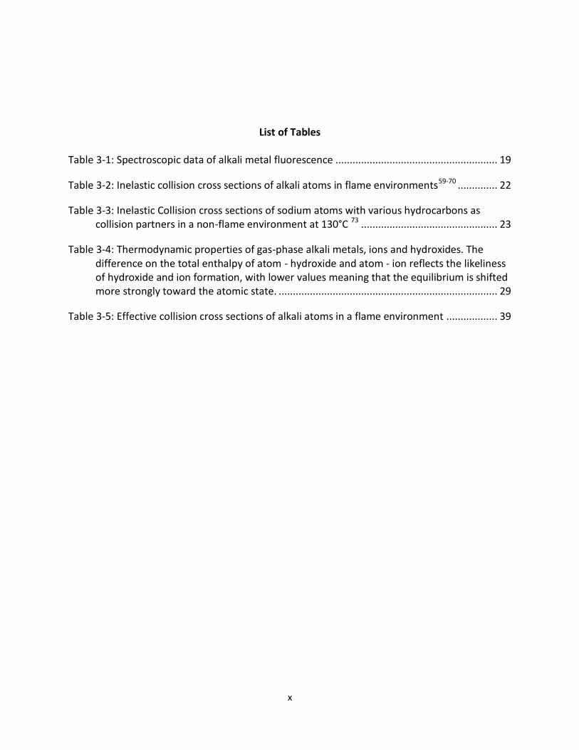
List of Tables ................................................................................................................................................x

List of Appendices ....................................................................................................................................... xi

List of Abbreviations .................................................................................................................................. xii

Abstract .................................................................................................................................................... xiii

CHAPTER 1. Background ......................................................................................................................... 1

1.1 Internal combustion engines ....................................................................................................... 1

1.2 Outline of this thesis ................................................................................................................... 4

CHAPTER 2. Underlying quantum mechanics for combustion spectroscopy .......................................... 7

2.1 The hydrogen atom wave function ............................................................................................. 7

2.1.1 The relativistic correction of the energy spectrum ........................................................... 10

2.1.2 Spin-orbit coupling ............................................................................................................ 11

2.1.3 The fine structure of the hydrogen atom .......................................................................... 13

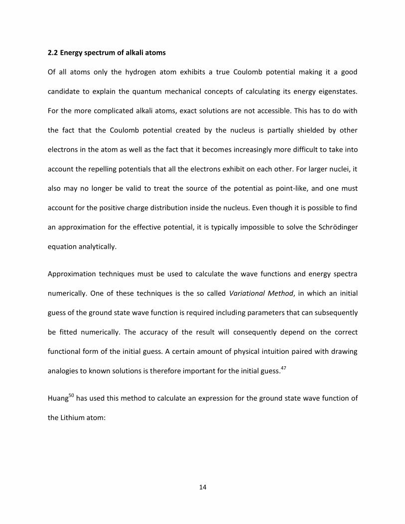
2.2 Energy spectrum of alkali atoms ............................................................................................... 14

2.3 Spontaneous emissions of light and selection rules for optical transitions ............................... 16

CHAPTER 3. Spectroscopic analysis of alkali metals in flames .............................................................. 19

3.1 Radiative and collisional energy transfer processes of alkali atoms in flames .......................... 19

3.2 Influence of the chemical environment on thermodynamic equilibrium .................................. 26

3.3 Assessment of self-absorption and line broadening of alkali fluorescence ............................... 36

3.3.1 Beer-Lambert law .............................................................................................................. 36

3.3.2 Natural line broadening .................................................................................................... 37

3.3.3 Collision line broadening ................................................................................................... 38

3.3.4 Doppler line broadening.................................................................................................... 39

3.3.5 Combination of line broadening effects and calculation of self-absorption ...................... 40

v

3.4 Other factors that influence alkali metal fluorescence intensity............................................... 46

3.5 Selection of suitable alkali metals as fuel dopants .................................................................... 46

3.6 Model prediction of alkali fluorescence intensity in the engine ............................................... 48

CHAPTER 4. Burned gas temperature calculation in homogeneous engine environments ................... 53

4.1 Cylinder pressure derived heat release analysis ....................................................................... 53

4.2 Calculation of burned gas temperature using GT-Power two-zone model ............................... 54

CHAPTER 5. Alkali metal fluorescence imaging in the engine ............................................................... 65

5.1 Experimental setup and operating conditions .......................................................................... 65

5.2 Simultaneous burned gas temperature and equivalence ratio imaging .................................... 68

5.3 Discussion of measurement uncertainties ................................................................................ 79

5.4 Mass fraction of burned fuel imaging using the spatially integrated sodium fluorescence ...... 85

CHAPTER 6. Application of alkali fluorescence imaging in stratified engine environments .................. 90

6.1 Individual cycle analysis in a spray-guided engine operation with high cyclic variations .......... 90

6.2 Improved experimental setup for spray-guided engine experiments ....................................... 93

6.3 Analysis of spray-guided, double-injected engine operation .................................................... 94

6.4 Analysis of the effect of different injectors on engine combustion .......................................... 97

CHAPTER 7. Conclusion and future potential of this technique for three dimensional measurements

and endoscope imaging in all-metal engines .................................................................................... 99

Appendices……………………………………………………………………………………………………………………………………….…103

References .............................................................................................................................................. 112

vi

List of Figures

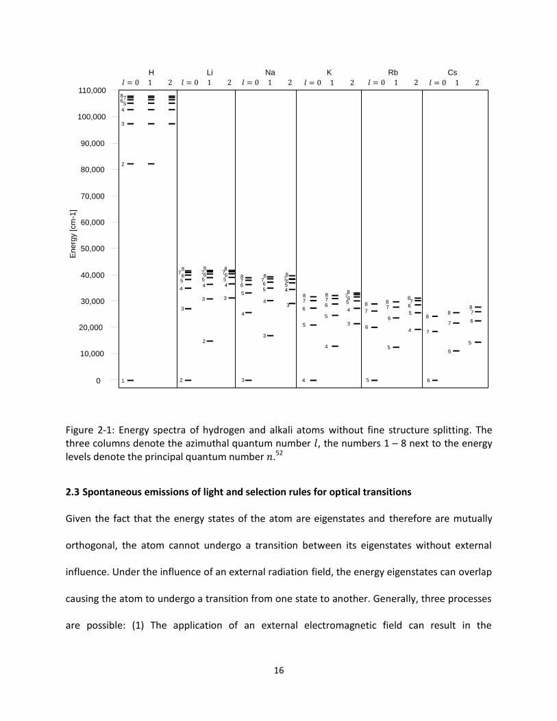
Figure 2-1: Energy spectra of hydrogen and alkali atoms without fine structure splitting. The three columns denote the azimuthal quantum number , the numbers 1 – 8 next to the energy levels denote the principal quantum number .52 ................................................. 16

Figure 3-1: Collisional excitation and relaxation and radiative relaxation via spontaneous emission of a photon ........................................................................................................... 21

Figure 3-2: The temperature dependent population of the lowest lying excited state of alkali metals can be calculated using the Boltzmann distribution law: .. 25

Figure 3-3: Temperature dependence of the ratio of the excited state populations Na/K and Na·Li/K2. ............................................................................................................................... 26

Figure 3-4: The calculated fraction of alkali metal atoms as a function of temperature,

pressure and equivalence ratio assuming chemical equilibrium with their oxidation

products. ............................................................................................................................. 31

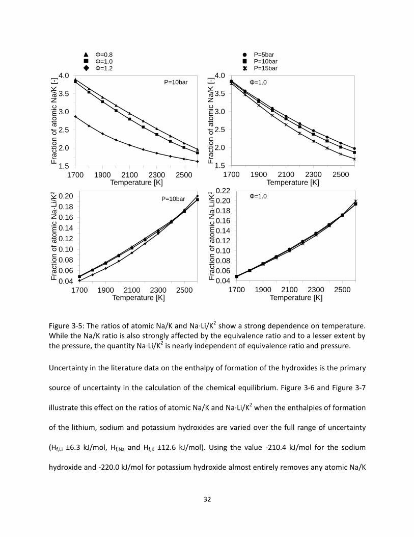
Figure 3-5: The ratios of atomic Na/K and Na·Li/K2 show a strong dependence on temperature. While the Na/K ratio is also strongly affected by the equivalence ratio and to a lesser extent by the pressure, the quantity Na·Li/K2 is nearly independent of equivalence ratio and pressure. ....................................................................................................................... 32

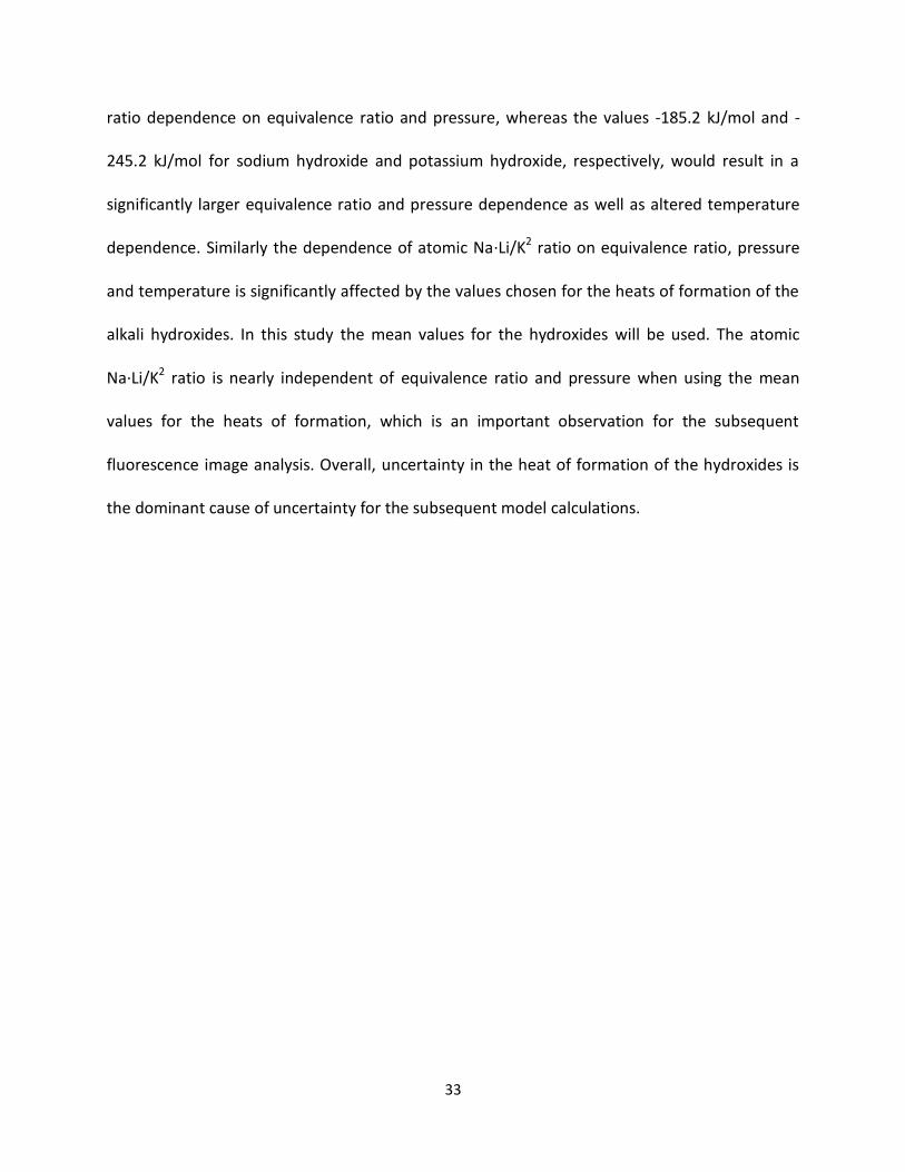
Figure 3-6: The chemical equilibrium of atomic Na/K and Na·Li/K2 for three combinations of enthalpies of formation as a function of temperature and a constant pressure of 10 bar and for equivalence ratios of Φ=0.8 and Φ=1.2. The values for the enthalpies of formation were selected as the mean and the two extreme values of the reported uncertainties in Table 3-4. ............................................................................................................................. 34

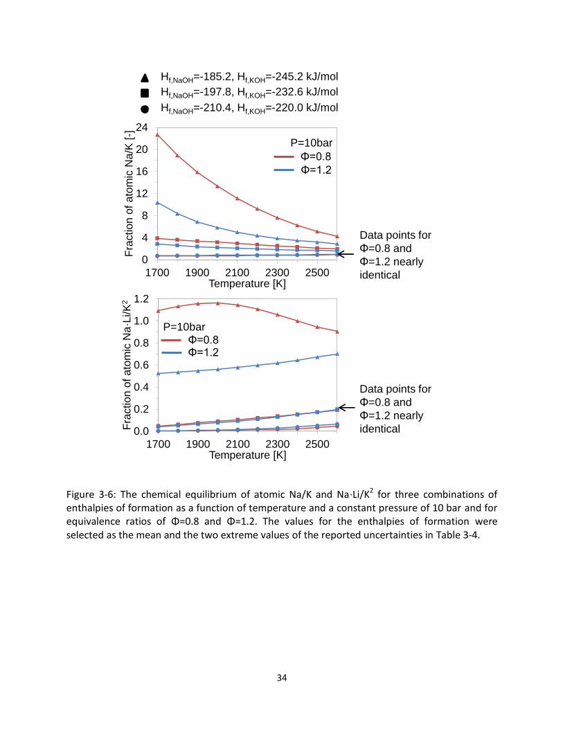
Figure 3-7: The chemical equilibrium of atomic Na/K and Na·Li/K2 is plotted for three combinations of enthalpies of formation as a function of temperature and a constant equivalence ratio of 1.0 and for pressures of P=5bar and P=15bar. The values for the enthalpies of formation were selected as the mean and the two extreme values of the reported uncertainties in Table 3-4. ................................................................................... 35

Figure 3-8: Spectral absorption and emission profile of Li, Na, K, Rb, and Cs atoms for various pressures and temperature. The plots stress the importance of calculating line broadening and absorption of fluorescence light individually for each data point at its corresponding pressure and temperature. ......................................................................... 41

vii

Figure 3-9: The fraction of re-absorbed light by ground state alkali atoms depends on gas temperature and pressure as a result of temperature and pressure dependent line broadening. In this calculation the mole fraction of alkali atoms in the burned gas zone were assumed as 400 ppm for each alkali species. ............................................................ 44

Figure 3-10: The ratio of the transmitted fluorescence light Na·Li/K2 and Na/K as a function of temperature for a range of pressures (P=5-20 bar) and atomic mole fractions in the burned gas (x=20-800 ppm). ............................................................................................... 45

Figure 3-11: Temperature and equivalence ratio dependence of the fluorescence intensity ratio Na/Li, Li/K, Na/K and Na·Li/K2. ............................................................................................ 50

Figure 3-12: Temperature and pressure dependence of the fluorescence intensity ratio Na/Li, Li/K, Na/K and Na·Li/K2. ....................................................................................................... 51

Figure 4-1: The crank angle resolved MFB is calculated from the recorded cylinder pressure trace using an in-house heat release analysis tool provided by General Motors .............. 54

Figure 4-2: Calculated burned gas temperatures using 'WoschniSwirl' heat transfer model and a convective heat transfer multiplier of 1.35. Small values of MFB result in a unrealistic calculated burned gas temperature early in the cycle. Setting an artificial threshold of 1% MFB for the temperature calculation still results in an unphysical initial spike, while a 2% MFB threshold produces an intuitively reasonable temperature curve. In all three cases the calculated burned gas temperatures are nearly identical after TDC............................ 56

Figure 4-3: The caluated burned gas temperatures depend on the heat transfer sub-model selection in GT-Power. The heat transfer sub-model selection can account for a deviation of the burned gas temperature of up to 75K. Although there is no quantitative justification for either one of the sub-models, the ‘WoschniSwirl’ model was used for all temperature calculations in this study................................................................................ 58

Figure 4-4: The calculated burned gas temperature is strongly affected by the value of the convective heat transfer multiplier (CHTM) in GT-Power. As expected, a lower multiplier values result in a higher calculated burned gas temperature. The value 1.35 was chosen for all temperature calculations in this study in agreement with the GT-Power help files and accounting for the high swirl motion in the combustion chamber due to the deactivation of one intake valve. ........................................................................................ 59

Figure 4-5: Selection of various heat transfer sub-models has little influence on the calculated cylinder pressure. The calculated pressures all differ up to 1 bar from the measured cylinder pressure early in the cycle and are in good agreement with the measurement after 30° aTDC. .................................................................................................................... 60

Figure 4-6: The cylinder wall, cylinder head and piston temperature were set to 325K, 400K and 450K (T1), 425K, 500K, 550K (T2) and 525K, 600K, 650K (T3) in the GT-Power calculation

viii

and the resulting calculated cylinder pressure is compared to the measured cylinder pressure trace. ..................................................................................................................... 62

Figure 4-7: (a) Running the GT-Power two-zone model in cylinder pressure (CP) mode produces a simulated cylinder pressure trace that is generally in better agreement with the measured pressure trace than in the mass fraction burned (MFB) mode. However, the results depend on the residual burned gas fraction (Res), which has to be input manually in CP mode while it is calculated as 12.4% in MFB mode. (b) The calculated burned gas temperature depends strongly on the residual burned gas fraction. The observation that the calculate temperature in CP mode with 12.4% residual fraction is slightly lower than in MFB mode, although the simulated cylinder pressure is higher. ....................................... 63

Figure 5-1: Experimental setup for the simultaneous high-speed imaging of lithium, sodium and potassium fluorescence ...................................................................................................... 67

Figure 5-2: Measured transmission spectra of the lens mounted bandpass filters with FWHM of 10 nm used during homogeneous engine operation. ......................................................... 68

Figure 5-3: Simultaneously recorded sodium, lithium and potassium fluorescence of a single engine cycle under homogeneous operating conditions at an equivalence ratio of Φ=1.06. The images show strong temporal and spatial intensity gradients due to their dependence on mass fraction of burned fuel and depth of the burned gas zone. ................................. 70

Figure 5-4: The fluorescence ratio (Na·Li)/K2 only depends on burned gas temperature and appears spatially much more homogeneous than the images in Figure 5-3. The Na/K ratios depend on burned gas temperature, cylinder pressure and equivalence ratio and also appear spatially more homogeneous than the images in Figure 5-3. ................................ 71

Figure 5-5: The vertical profiles of the fluorescence intensity of lithium, sodium and potassium and the fluorescence intensity ratios Na/K and Na·Li/K2 in Figure 5-3 and Figure 5-4 were taken immediately to the right of the masked out spark plug at 2° aTDC. The fluorescence intensities show large spatial gradients, whereas the intensity ratios appear much more homogeneous. ..................................................................................................................... 72

Figure 5-6: Experimental measurements of cylinder pressure and relative atomic alkali metal fluorescence intensities and intensity ratios from 12° - 70° aTDC in a nearly homogeneously operated engine. Comparison with predicted atomic fluorescence intensities and intensity ratios show good agreement over a wide range of conditions. The error bars of ±100 K in parts (e) and (f) represent the estimated accuracy uncertainty of the GT-Power temperature calculation. ............................................................................. 75

Figure 5-7: Simultaneous imaging of burned gas temperature and equivalence ratio after the recorded alkali fluorescence intensities were post-processed. The numbers in the top left corner of each image denote the measured cylinder pressure and crank angle position.

ix

The rectangular and circular black areas in the center of the images mask out the spark plug ground strap and a dust grain on one of the camera chips, respectively. .................. 76

Figure 5-8: Comparison of calculated burned gas temperature using the GT-Power two-zone model and the spatial average of the measured burned gas temperature of Figure 5-7 using the Li·Na/K2 fluorescence intensity ratio. An overall accuracy uncertainty is estimated as ±100 K due to various assumptions in the zero dimensional GT-Power model. .................................................................................................................................. 79

Figure 5-9: The calculated equivalence ratio of an early flame kernel assuming that (a) the depth of the burned gas cloud is fully expanded and the absorption path length is maximum and (b) complete absence of absorption. .......................................................... 81

Figure 5-10: Sodium fluorescence images of the early flame kernel in a homogeneous, stoichiometric engine operation. The numbers in the left and right upper corners of the images denote crank angle position aTDC and MFB, respectively. No mask was applied to cover the spark plug electrode to minimize error in the subsequent spatial integration of the sodium signal. However, the presence of the spark plug electrode introduces uncertainty especially for small flame kernels. ................................................................... 86

Figure 5-11: (a) The spatially integrated sodium fluorescence intensities show a large spread for different engine operating conditions. (b) The spatially integrated sodium fluorescence intensities collapse onto the same curve with an uncertainty of MFB ±0.02, after the fluorescence signal was corrected for its temperature, pressure, equivalence ratio and absorption dependence. ..................................................................................................... 88

Figure 6-1: Comparison of temperature and equivalence ratio of a well burning and partially burn combustion cycle. ....................................................................................................... 92

Figure 6-2: Measured transmission spectra of the lens mounted bandpass filters with FWHM of 1 nm and 2 nm, respectively, used during stratified engine operation to suppress soot luminosity. ........................................................................................................................... 94

Figure 6-3: Measured burned gas temperature and equivalence ratio of an ensemble averaged, double-injected, stratified combustion event. ................................................................... 96

Figure 6-4: Comparison of measured burned gas temperature and equivalence ratio of ensemble averaged, single injected, stratified engine combustion cycles using two different injectors. ............................................................................................................... 98

x

List of Tables

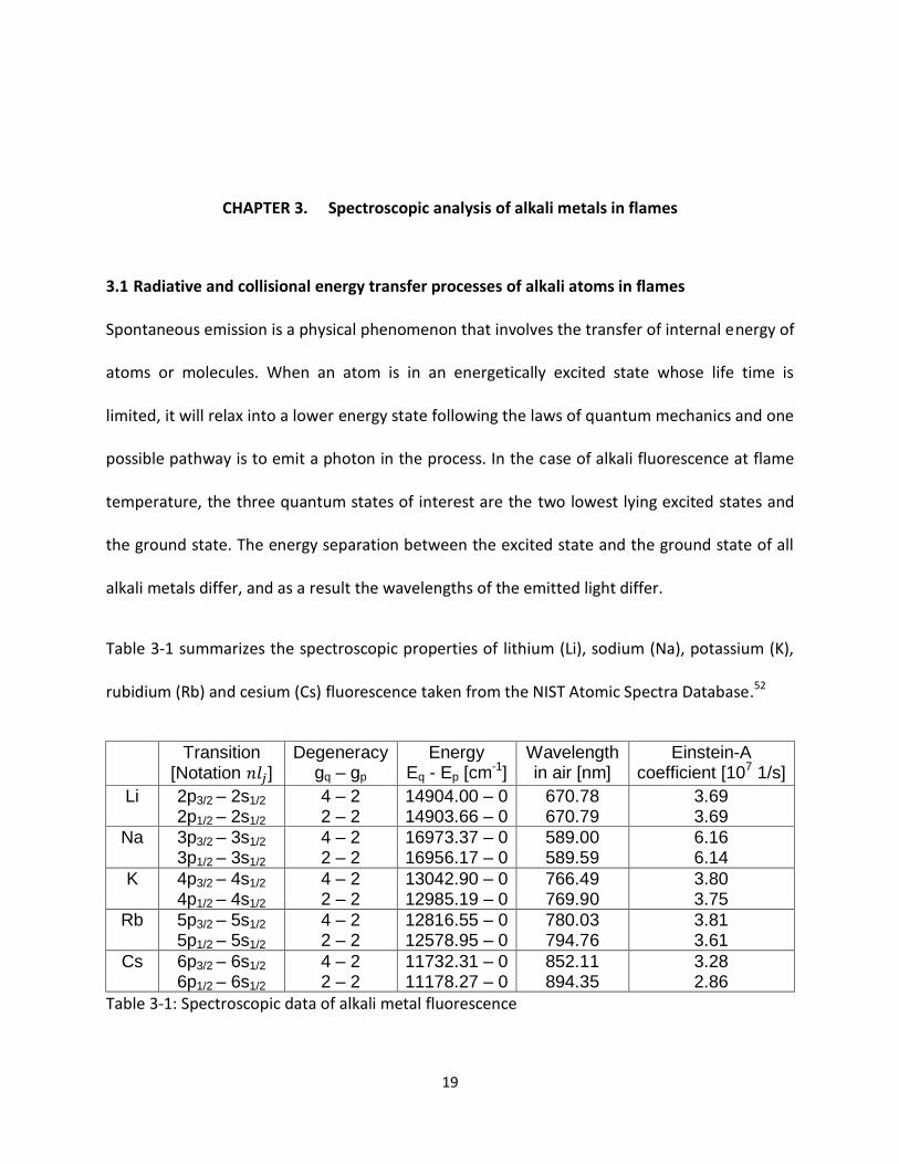
Table 3-1: Spectroscopic data of alkali metal fluorescence ......................................................... 19

Table 3-2: Inelastic collision cross sections of alkali atoms in flame environments59-70 .............. 22

Table 3-3: Inelastic Collision cross sections of sodium atoms with various hydrocarbons as collision partners in a non-flame environment at 130°C 73 ................................................ 23

Table 3-4: Thermodynamic properties of gas-phase alkali metals, ions and hydroxides. The difference on the total enthalpy of atom - hydroxide and atom - ion reflects the likeliness of hydroxide and ion formation, with lower values meaning that the equilibrium is shifted more strongly toward the atomic state. ............................................................................. 29

Table 3-5: Effective collision cross sections of alkali atoms in a flame environment .................. 39

xi

List of Appendices

Appendix A: Absorption calculation macro .............................................................................. 103

Appendix B: Flow chart for building fluorescence intensity database .................................... 108

Appendix C: Flow chart of image processing ............................................................................ 109

Appendix D: T and Ф measurements using photo-multipliers ................................................. 110

xii

List of Abbreviations

aTDC: After Top Dead Center

bTDC: Before Top Dead Center

CA: Crank Angle

CHTM: Convective Heat Transfer Multiplier

COV: Coefficient of Variance

EGR: Exhaust Gas Recirculation

EOI: End of Injection

FWHM: Full-Width at Half-Maximum

IMEP: Indicated Mean Effective Pressure

LIF: Laser Induced Fluorescence

MFB: Mass Fraction of Burned Fuel

P: Pressure

Φ: Equivalence Ratio

RMS: Root Mean Squared

SIDI: Spark-Ignition Direct-Injection

SI-PFI: Spark-Ignition Port-Fuel-Injection

T: Temperature

TDC: Top Dead Center

xiii

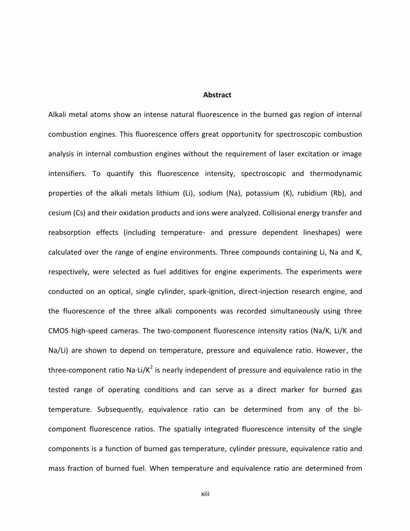
Abstract

Alkali metal atoms show an intense natural fluorescence in the burned gas region of internal

combustion engines. This fluorescence offers great opportunity for spectroscopic combustion

analysis in internal combustion engines without the requirement of laser excitation or image

intensifiers. To quantify this fluorescence intensity, spectroscopic and thermodynamic

properties of the alkali metals lithium (Li), sodium (Na), potassium (K), rubidium (Rb), and

cesium (Cs) and their oxidation products and ions were analyzed. Collisional energy transfer and

reabsorption effects (including temperature- and pressure dependent lineshapes) were

calculated over the range of engine environments. Three compounds containing Li, Na and K,

respectively, were selected as fuel additives for engine experiments. The experiments were

conducted on an optical, single cylinder, spark-ignition, direct-injection research engine, and

the fluorescence of the three alkali components was recorded simultaneously using three

CMOS high-speed cameras. The two-component fluorescence intensity ratios (Na/K, Li/K and

Na/Li) are shown to depend on temperature, pressure and equivalence ratio. However, the

three-component ratio Na·Li/K2 is nearly independent of pressure and equivalence ratio in the

tested range of operating conditions and can serve as a direct marker for burned gas

temperature. Subsequently, equivalence ratio can be determined from any of the bi-

component fluorescence ratios. The spatially integrated fluorescence intensity of the single

components is a function of burned gas temperature, cylinder pressure, equivalence ratio and

mass fraction of burned fuel. When temperature and equivalence ratio are determined from

xiv

the fluorescence intensity ratios, the spatially integrated fluorescence signal of sodium can

serve as a marker for the mass fraction of burned fuel.

The tool was applied to various cases of direct injected, stratified engine combustion to

illustrate the potential of this technique for optimization of the combustion strategy and engine

hardware configuration.

1

CHAPTER 1. Background

1.1 Internal combustion engines

The internal combustion engine has become the primary propulsion source for personal

transportation. High energy density of the fuel, the wide spread availability of fuel as well as

large advances in vehicle tailpipe emissions over the past decades make it the preferred

propulsion concept of our days. Fuel price, environmental concerns as well as the legislation in

many parts of the world demand further improvement of emissions and fuel economy in the

future. To achieve and exceed these demands automakers are working on the continuous

improvement of existing combustion concepts to improve energy efficiency and lower tailpipe

emissions.

During the past decades the most common gasoline combustion concept was the spark-

ignition, port-fuel-injection (SI-PFI) gasoline engine. For this engine, the fuel is injected into the

intake port just upstream the intake valve, where it evaporates and the gaseous air-fuel mixture

enters the combustion chamber. Because the air-fuel mixture is only ignitable by spark within a

narrow range of nearly stoichiometric equivalence ratios, engine load must be controlled by

choking the air flow. A great benefit from stoichiometric engine operation is that it allows for

the use of a three way catalyst downstream the exhaust port to chemically convert the

combustion products carbon monoxide, nitrogen oxides and unburned hydrocarbons into

2

carbon dioxide, nitrogen and water. However, the need for a stoichiometric equivalence ratio

causes the SI-PFI engine to have low combustion efficiency particularly at low load operating

conditions.1

In recent years the SI-PFI has partly been replaced by the introduction of the spark ignited,

direct injected (SIDI) gasoline engine. This engine injects the fuel directly into the combustion

chamber where it evaporates and mixes with the air. This method allows for load control by

controlling only the amount of fuel injected whereas the air flow remains unrestricted. To

overcome the issue of ignitability of the very lean air fuel ratios at low load operating

conditions, various fuel stratification methods have been developed to create a cloud of nearly

stoichiometric equivalence ratio at or in close proximity to the spark plug while the overall

equivalence ratio remains lean. These methods encompass wall and air guided injection

systems, where the injector typically sits far from the spark plug and the fuel cloud is

transported to the spark plug by proper design of the piston wall or the flow field inside the

engine to transport the fuel cloud close to the spark plug. Spray guided systems have the

injector positioned close to the spark plug spraying the fuel onto or close to the spark plug.1

A downside of stratified SIDI engine operation is the need for a much more complex exhaust

gas after-treatment system in comparison to the three-way catalyst. The need for reduction of

nitrogen oxides to meet emission regulations may necessitate the use of expensive lean NOx

traps or selective catalytic reduction catalysts. A better solution would be to prevent the

formation of nitrogen oxides in the engine in the first place. This can be achieved by lowering

the combustion temperature by recirculating exhaust gas (EGR) back into the air intake,

3

because the formation of nitrogen oxides in the flame strongly depends on temperature. The

higher specific heat of carbon dioxide and water2 contained in the exhaust gas helps reduce

peak combustion temperatures and reduce the formation of nitrogen oxides.1

Especially with high rates of EGR, stratified SIDI engine combustion suffers from occasional,

random misfires and partial burns. These pose a large problem for both engine efficiency and

emissions, because large amounts of hydrocarbons from the fuel exit the engine unburned. Up

to date there is no comprehensive understanding of what causes these cycle to cycle variations

and how to avoid them effectively.

Double or multiple injections per engine cycle can improve combustion stability and lower

tailpipe emissions and can be utilized as an exhaust gas heating strategy for cold start

operation.1, 3-6 Increased soot formation when injecting into the flame poses a potential

limitation to this strategy, because the emission of particulate matter is regulated by legislation.

Quantitative knowledge of local temperature and equivalence ratio is often desired to optimize

engine operating parameters and combustion chamber design. The global equivalence ratio can

be obtained from a carbon and oxygen analysis of exhaust species such as CO, CO2, H2O, O2,

NOx 7 or the use of wide-range exhaust oxygen sensors.8 However, these devices cannot provide

the spatial and temporal resolution that is necessary in the highly dynamic and spatially

stratified environment of direct injection engines. The fast response sampling of gas from the

cylinder can provide better temporal resolution but no spatial resolution.9-12 Various studies

have attempted one or two dimensionally resolved measurements of fuel concentration or

air/fuel ratio in the cylinder of operating engines using optical diagnostics. These techniques

4

include infrared absorption spectroscopy13, 14, ion-current sensing at the spark plug15-17,

chemiluminescence imaging of combustion radicals such as OH, CH, C2 and CN18-23, laser

induced fluorescence (LIF)24-33 and laser Raman scattering.26, 34 The experimental uncertainty of

these tools is typically near ±10%. Fansler et al.23 summarize the specific advantages and

disadvantages of each technique with respect to spatial and temporal measurement resolution,

potential for quantifying the local equivalence ratio and limitation to certain areas of interest

such as the spark plug.

The application of optical diagnostics in engines is often limited by costly and sensitive

equipment such as lasers and image intensifiers (LIF, Raman spectroscopy), the limitation to

flame front processes (OH, CH and C2 chemiluminescence) or restriction to areas near the spark

plug (ion current sensing, CN chemiluminescence). Infrared absorption techniques can only

provide measurements that are averaged along the line of sight, while LIF and Raman

spectroscopy are limited to two dimensional planar measurements. Despite the large advances

in our understanding of engine combustion in the past, there is still strong demand for reliable

measurement techniques that can overcome some of the limitations of currently available

tools. It is desirable to extend the toolset of optical diagnostics toward lower hardware

requirements so it can be used reliably in industrial research and product development

environments.

1.2 Outline of this thesis

The scope of this thesis is to develop a technique that will allow the high-speed measurement

of burned gas temperature (T), equivalence ratio (Φ) and mass fraction of burned fuel (MFB) in

5

an internal combustion engine using alkali metal spectroscopy with two-dimensional spatial

resolution. While most other optical diagnostic tools determine equivalence ratio from the

measurement of fuel concentration in the unburned zone, this tool will allow for monitoring the

spatial and temporal evolution of equivalence ratio in the burned zone to aid the understanding

of in-cylinder pollutant and soot oxidation late in the combustion cycle. The tool will also

minimize cost and complexity of the measurement apparatus, so it can be readily applied to the

improvement of next-generation internal combustion engines in industrial engine development

environments.

Alkali metals can be introduced into the combustion chamber as air seeding or fuel dopants.

The high temperatures in the flame and burned gas region excite the alkali atoms and the

subsequent fluorescence can be strong enough to be captured with standard, high-speed

cameras without the need for image intensifiers or lasers. The intensity of the alkali

fluorescence light in the burned gas region mainly depends on the number of alkali atoms

present, the fraction of the atoms that are present in an excited electronic state, the transition

probability between excited state and ground state as well as the reabsorption of emitted light

by ground-state alkali atoms. The total number of atoms can vary as a function of the air to fuel

ratio, because an increased availability of oxygen and hydroxyl radicals will affect the chemical

reactions that bind the free atoms into various molecules. The fraction of the atoms that are

present in an excited state depends on the gas temperature, while the transition probability is a

constant of nature and cannot be manipulated. The self-absorption of the fluorescence mainly

depends on the number density of ground-state alkali atoms, the absorption path length and

6

the spectral absorptivity, which is strongly influenced by various ways of absorption line

broadening.

Sodium luminescence has first been utilized in engine experiments for combustion analysis in

1935-1940 by Rassweiler et al.35-37, Withrow et al.38, 39 and Brevoort40, where the intake air of a

spark-ignited gasoline engine was seeded with sodium salt to visualize flame propagation and

measure combustion temperature using the sodium line reversal method. Drake et al.41 and

Zeng et al.42 utilized sodium luminosity in a spray-guided, spark ignited, direct injection gasoline

engine to visualize early flame propagation. Most recently, Beck et al.43 and Reissing et al.44

doped the fuel with sodium and potassium and utilized the temperature dependence of the

sodium to potassium fluorescence ratio to calculate burned gas temperature. In all studies the

influence of the chemical environment, the collisional environment as well as self-absorption of

the fluorescence light was not considered. The applicability of this tool was therefore limited to

a narrow range of operating conditions.45 In order to verify critical assumptions and to obtain

better quantitative information from this technique by considering the effects of pressure and

local equivalence ratio on the alkali signals, it is indispensable to conduct a thorough,

quantitative examination of all physical processes involved.

The purpose of this research is to investigate the effect of various physical and chemical

processes on the fluorescence intensities of various alkali metals and to find ways to utilize the

fluorescence of three alkali metals quantitatively and reliably as a high-speed measurement

tool for local burned gas temperature, equivalence ratio and the burned fuel mass fraction in an

internal combustion engine under a wide range of operating conditions.

7

CHAPTER 2. Underlying quantum mechanics for combustion spectroscopy

Combustion spectroscopy can help gain better insight into some combustion parameters that

influence engine performance and emissions. Many phenomena that are relevant to

combustion spectroscopy occur on a molecular or atomic level and cannot be explained by

classical physics. Since atomic spectroscopy is based on the transition of electrons between

various energy levels in the atom, one must understand the quantum mechanical nature of the

energy spectra of atoms. This chapter shall provide an overview of the underlying physics of

atomic spectroscopy, which is detrimental to understand and interpret the observed alkali

metal fluorescence in a combustion engine correctly. Since alkali metals are the elements in the

first group of the periodic system, their electronic structure with one electron in the outermost

shell is similar to the electronic structure of the hydrogen atom. It is easiest to analyze the

energy spectrum of the hydrogen atom, because it only possesses one electron in total,

whereas alkali atoms also have various layers of inner electrons shielding the potential of the

nucleus on the outer electron.46

2.1 The hydrogen atom wave function

A wave function describes the wave-like nature of atomic and sub-atomic particles. It contains

all information such as position, momentum or internal energy of the particle and must satisfy

the Schroedinger equation, which is the quantum mechanical analogy to Newton’s laws in

8

classical physics and describes the time evolution of the wave function. The time independent

Schroedinger equation for an electron in spherical coordinates is given in Equation [2-1].

[

(

)

(

)

(

)] [2-1]

where is Planck’s constant, is the electron mass, is the electron wave function, is the

the radial distance of the electron from the nucleus, and are the spherical angles, and the

potential the electron is subject to. The operator

denotes the Hamiltonian with

energy eigenvalue .

The nucleus of the hydrogen atom consists of one positively charged proton exhibiting a

Coulomb potential. Orbiting this nucleus is the negatively charged electron.

The Coulomb potential for the hydrogen atom reads as follows:

( )

[2-2]

where is the electric charge of the electron and proton and the vacuum permittivity. A

first-order approximation of the solution to the hydrogen wave function is derived in various

quantum mechanics textbooks.47-49 For the ground state of the hydrogen atom the wave

function reads as:

( ) ( ) ( )

√

[2-3]

9

where

is the Bohr radius. For higher quantum states, the

expression can be generalized to: 48

( ) √(

) ( )

[( ) ]

(

)

[ (

)]

( ) [2-4]

where is the principal quantum number, the azimuthal quantum number, (

) are

the associated Laguerre polynomials and ( ) are the spherical harmonics of the form:48

( ) √( )

( | |)

( | |)

( ) [2-5]

where is the magnetic quantum number and with ( )

The potential energy of the hydrogen electron is also derived in various textbooks47-49 and is

expressed by the following equation:

[

(

)

]

[2-6]

It is apparent from Equation [2-6] that the electronic energy calculated to this order depends

only on the principal quantum number and not on the orbital angular momentum denoted by

the quantum numbers and . Further considerations of relativistic corrections, as well as the

spin angular momentum of the electron, lift this degeneracy.

10

2.1.1 The relativistic correction of the energy spectrum

The first term of the Hamiltonian in Equation [2-1],

, denotes kinetic energy.

[2-7]

One can relate the classical expression for kinetic energy to the quantum mechanical

expression. The classical formula for relativistic kinetic energy is:

√ ( )

[2-8]

where is the kinetic energy, denotes the classical velocity and the speed of light in

vacuum. Since the classical concept of velocity does not exist in quantum mechanics, Equation

[2-8] needs to be expressed in terms of momentum and expanded in a power series.

[√ (

)

] [

(

)

(

)

] [2-9]

where denotes momentum. Disregarding all higher order corrections results in an expression

for the relativistic correction term of the Hamiltonian and consequently in a correction term for

the energy eigenvalue:48

[2-10]

11

[

(

)

(

)

( )

] [2-11]

The fact that the azimuthal quantum number appears in this correction resolves the

previously existing degeneracy of the energy spectrum in .

2.1.2 Spin-orbit coupling

The spin of the electron is another quantum mechanical subtlety that does not exist in classical

physics but needs to be considered here. Spin is a form of angular momentum that is intrinsic

to many quantum particles such as the electron. In quantum mechanics, the spin angular

momentum of a particle can be characterized by two quantum numbers, and . While

gives information about the magnitude of the spin angular momentum, provides

information about the direction. This notation is analogous to the quantum numbers used for

orbital angular momentum, and . Spin becomes important in the calculation of the energy

levels of an atom when the magnetic field of the proton acts on the orbiting electron and forces

it to align its magnetic moment along the direction of the field. Therefore one must add a

correction term to the Hamiltonian of Equation [2-1] of the form:

→ [2-12]

Where is the magnetic dipole moment of the electron and → the magnetic field. The

magnetic field can be described as:

12

→

→ [2-13]

where → is the orbital angular momentum operator, and the magnetic dipole moment of the

electron is:

→ [2-14]

with → as the spin angular momentum operator. Putting it together and considering Thomas

precession48, which adds another factor of ⁄ to the equation, results in an expression for the

spin-orbit perturbation of the original Hamiltonian of the form: 48

→

→ [2-15]

The consequence of considering spin-orbit interaction is that the orbital and spin angular

momenta of the electron are no longer conserved separately and the magnetic quantum

number as used in the derivation of the solution to the angular part of the wave function as

well as are no longer conserved quantities. However, it can be shown that the new

eigenstates of the perturbed Hamiltonian are also eigenstates of the total angular momentum.

→ → → [2-16]

Equation [2-16] gives rise to a new quantum number for total angular momentum , with

( ) ( ). Using this, one can derive the correction term to the hydrogen energy

eigenvalues as:48

13

(

) [2-17]

2.1.3 The fine structure of the hydrogen atom

Combining both relativistic correction and the spin-orbit interaction, the solution to the new

Hamiltonian in the Schrödinger equation can be rewritten with better accuracy and now

depends not only on the principle quantum number but also on the quantum number for total

angular momentum : 48

[

(

)] [2-18]

In summary, the consideration of relativistic corrections to the kinetic term of the Hamiltonian

as well as spin-orbit interaction results in the fine structure of the atomic energies that are no

longer degenerate in . Rather, Equation [2-18] takes into account the contribution of total

angular momentum to the energy eigenvalues, and eigenstates of different total angular

momentum now differ in energy. It shall be noted that the new eigenstates are also eigenstates

of the original Hamiltonian of Equation [2-1], and one can now also introduce a new quantum

number to replace , which can accordingly take on values in the interval

| | . Besides this change, the equations for the spherical harmonics and the solution to the

angular part of the wave function remain the same. Since the solution to the angular part of the

wave function has no contribution to the energy eigenvalues, the energy spectrum is still

degenerate in .

14

2.2 Energy spectrum of alkali atoms

Of all atoms only the hydrogen atom exhibits a true Coulomb potential making it a good

candidate to explain the quantum mechanical concepts of calculating its energy eigenstates.

For the more complicated alkali atoms, exact solutions are not accessible. This has to do with

the fact that the Coulomb potential created by the nucleus is partially shielded by other

electrons in the atom as well as the fact that it becomes increasingly more difficult to take into

account the repelling potentials that all the electrons exhibit on each other. For larger nuclei, it

also may no longer be valid to treat the source of the potential as point-like, and one must

account for the positive charge distribution inside the nucleus. Even though it is possible to find

an approximation for the effective potential, it is typically impossible to solve the Schrödinger

equation analytically.

Approximation techniques must be used to calculate the wave functions and energy spectra

numerically. One of these techniques is the so called Variational Method, in which an initial

guess of the ground state wave function is required including parameters that can subsequently

be fitted numerically. The accuracy of the result will consequently depend on the correct

functional form of the initial guess. A certain amount of physical intuition paired with drawing

analogies to known solutions is therefore important for the initial guess.47

Huang50 has used this method to calculate an expression for the ground state wave function of

the Lithium atom:

15

(

) [ ( )

] [ ( )

]

(

) [

( )

] [

( ) ]

[2-19]

This yielded an energy value of the 2s ground state to be in agreement with experimental

values within an error of 0.5%. In a more recent study by Guevara et al. 51, who used a seven

parameter estimate of the wave function, the ground state energy could be calculated to within

.06% of the experimental value. It must be noted that the use of the variational method can

often yield very good approximations of the ground state energy, but this does not necessarily

mean that one has found an accurate description of the wave function that can be used for

calculating transition rates.47 For the purpose of atomic spectroscopy on alkali atoms as a tool

to conduct combustion analysis, it is therefore necessary to rely on experimentally determined

values of energies and transition rates. Figure 2-1 shows the energy spectra of hydrogen and

alkali atoms taken from the Atomic Spectra Database of the National Institute for Standards

and Technology (NIST).52

16

Figure 2-1: Energy spectra of hydrogen and alkali atoms without fine structure splitting. The three columns denote the azimuthal quantum number , the numbers 1 – 8 next to the energy levels denote the principal quantum number .52

2.3 Spontaneous emissions of light and selection rules for optical transitions

Given the fact that the energy states of the atom are eigenstates and therefore are mutually

orthogonal, the atom cannot undergo a transition between its eigenstates without external

influence. Under the influence of an external radiation field, the energy eigenstates can overlap

causing the atom to undergo a transition from one state to another. Generally, three processes

are possible: (1) The application of an external electromagnetic field can result in the

0

10,000

20,000

30,000

40,000

50,000

60,000

70,000

80,000

90,000

100,000

110,000

H Li Na K Rb Cs

En

erg

y [cm

-1]

1

2

3

4

56

78

2

2

3

3 3

44 4

5 5 56 6 67 7 78 8 8

3

3

4

34

45

556 667 7 78 8 8

4

4

4

5

5

5

66

67 7

78 88

5

5

5

6

6

67

77

8 88

6

6

6

7

7

78

88

3

4

5

17

absorption of a photon by the atom lifting its electron into a higher energy state. This can be

observed in laser induced fluorescence, where the laser is used as an excitation source for the

atom. (2) The application of an external electromagnetic field can cause stimulated emission by

causing the atom to release energy and fall down into a lower energy state emitting a photon

coherent with the external light source. Stimulated emission is the underlying process of light

amplification in a laser. (3) Finally, without application of an external electromagnetic field but

triggered by vacuum fluctuations of space itself, the atom can undergo a transition from a

higher into a lower energy state and emit the energy difference through the creation of a

photon with its frequency corresponding to the energy difference. This process is called

spontaneous emission and forms the underlying physics for the spectroscopic observations

discussed in this thesis.

The intensity of the emitted light depends largely on the rate on which transitions occur. The

transition rate depends on both the magnitude of the energy split as well as on the overlap of

both wave functions under the influence of the newly created photon. It can be summarized in

a quantity called the Einstein-A coefficient for spontaneous emission. An expression for it is

derived in Bransden and Hoachain49 as:

| | | | [2-20]

The Einstein-A coefficient can be calculated if one has accurate expressions for the wave

functions of both states involved. As discussed, this is not always possible for non-hydrogen

atoms with several electrons. But the Einstein-A coefficient for spontaneous emission is also the

18

inverse of the radiative lifetime of the excited state. It can therefore also be obtained

experimentally by lifetime measurements.

Simple rules can be derived from the evaluation of the matrix element in Equation [2-20]. The

ones important for atomic spectroscopy are:

[2-21]

The electron spin remains unaffected by the interaction with the electromagnetic field. With

this in mind it is important to emphasize that any transition into the ground state (s-orbital,

) of an alkali atom through spontaneous emission of one photon must originate from a p-

orbital ( ).

19

CHAPTER 3. Spectroscopic analysis of alkali metals in flames

3.1 Radiative and collisional energy transfer processes of alkali atoms in flames

Spontaneous emission is a physical phenomenon that involves the transfer of internal energy of

atoms or molecules. When an atom is in an energetically excited state whose life time is

limited, it will relax into a lower energy state following the laws of quantum mechanics and one

possible pathway is to emit a photon in the process. In the case of alkali fluorescence at flame

temperature, the three quantum states of interest are the two lowest lying excited states and

the ground state. The energy separation between the excited state and the ground state of all

alkali metals differ, and as a result the wavelengths of the emitted light differ.

Table 3-1 summarizes the spectroscopic properties of lithium (Li), sodium (Na), potassium (K),

rubidium (Rb) and cesium (Cs) fluorescence taken from the NIST Atomic Spectra Database.52

Transition [Notation ]

Degeneracy gq – gp

Energy Eq - Ep [cm-1]

Wavelength in air [nm]

Einstein-A coefficient [107 1/s]

Li 2p3/2 – 2s1/2

2p1/2 – 2s1/2 4 – 2 2 – 2

14904.00 – 0 14903.66 – 0

670.78 670.79

3.69 3.69

Na

3p3/2 – 3s1/2

3p1/2 – 3s1/2 4 – 2 2 – 2

16973.37 – 0 16956.17 – 0

589.00 589.59

6.16 6.14

K

4p3/2 – 4s1/2

4p1/2 – 4s1/2 4 – 2 2 – 2

13042.90 – 0 12985.19 – 0

766.49 769.90

3.80 3.75

Rb 5p3/2 – 5s1/2

5p1/2 – 5s1/2 4 – 2 2 – 2

12816.55 – 0 12578.95 – 0

780.03 794.76

3.81 3.61

Cs 6p3/2 – 6s1/2

6p1/2 – 6s1/2 4 – 2 2 – 2

11732.31 – 0 11178.27 – 0

852.11 894.35

3.28 2.86

Table 3-1: Spectroscopic data of alkali metal fluorescence

20

The letters ‘q’ and ‘p’ denote the excited state and the ground state, respectively, while the

Einstein-A coefficient denotes the rate constant of spontaneous emission. Because of the fine

structure energy splitting of the p-orbital (

), alkali atoms typically

show two emission lines at slightly differing wavelengths. The transmission on the shorter of

the two wavelengths is approximately twice as strong, because the ⁄ state is four-fold

degenerate in ⁄ ⁄ ⁄ ⁄ , while the state only carries a two-fold

degeneracy in ⁄ ⁄ .

Atoms and molecules in the gas phase possess kinetic energy, which is statistically distributed

according to the Maxwell-Boltzmann law of velocity distribution. The distribution is a function

of the gas temperature and can be described by Equ. [3-1].53

( ) (

)

[3-1]

where denotes the velocity, the mass of the atom, the Boltzmann constant and the

gas temperature. At elevated pressure and temperature atoms and molecules undergo

frequent collisions resulting in a transfer of energy from one collision partner to the other.

These collisions can be elastic, where the total kinetic energy of the collision partners is

conserved, or inelastic with part of the kinetic energy being transformed into internal, potential

energy and vice versa. The distribution of these quantized energy states is described by the

Boltzmann law shown in Equation [3-2].53

21

( )

( )

[3-2]

where denotes the degeneracy of eigenstate , is its potential energy eigenvalue, the

excitation temperature and ( ) the temperature dependent partition function. In a state of

thermal equilibrium, the gas temperature and excitation temperature are the same. If

however not all degrees of freedom are equilibrated, these temperatures can differ from one

another. It is important to examine whether the assumption of thermal equilibrium is valid for

hot alkali metal atoms in a combustion engine environment, when energy loss occurs via

radiation by spontaneous emission.

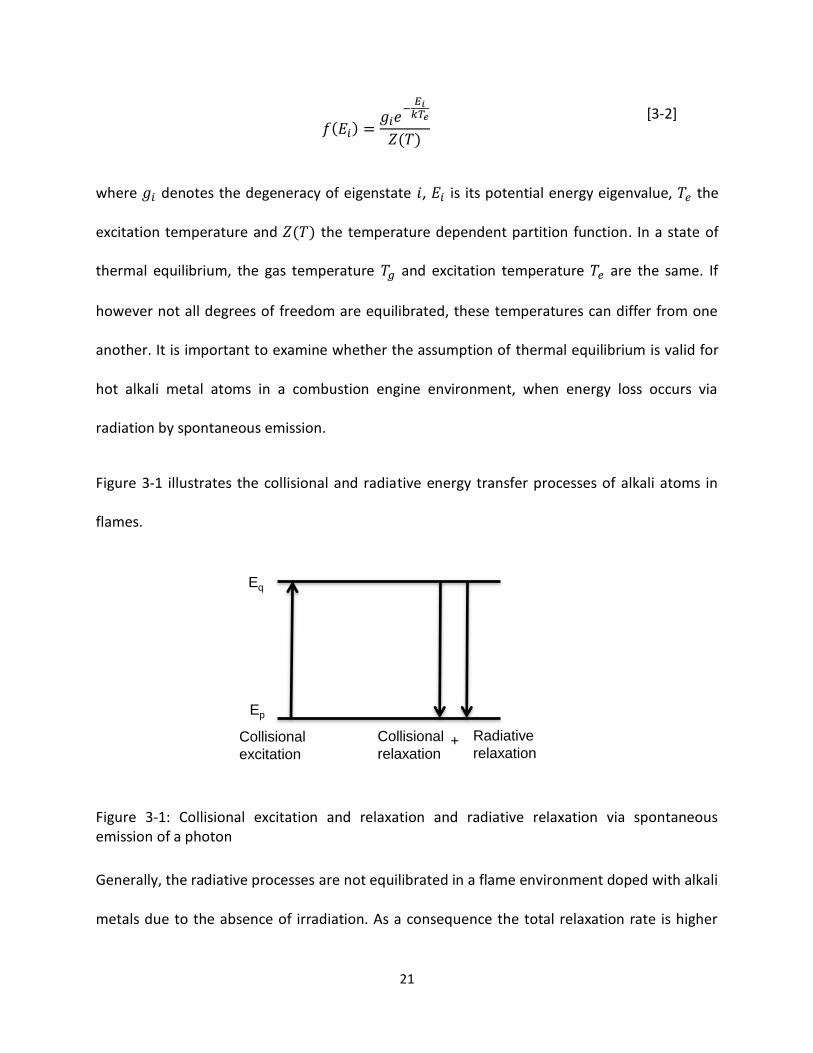
Figure 3-1 illustrates the collisional and radiative energy transfer processes of alkali atoms in

flames.

Figure 3-1: Collisional excitation and relaxation and radiative relaxation via spontaneous emission of a photon

Generally, the radiative processes are not equilibrated in a flame environment doped with alkali

metals due to the absence of irradiation. As a consequence the total relaxation rate is higher

Collisional

excitation

Collisional

relaxation

Radiative

relaxation+

Eq

Ep

22

than the collisional excitation rate and the system is not in a strict thermal equilibrium. If the

radiative energy loss is significant, this means that the population of the excited alkali states

cannot be described accurately by the Boltzmann law using the gas temperature. Rather, the

excited states would generally be under-populated resulting in the excitation temperature

being lower than the gas temperature. However, under the assumption that collisional

excitation and relaxation occur on a much faster time scale than the relaxation via radiation,

the distribution of the population of internally excited states follows Boltzmann statistics with

the excitation temperature being equal to the gas temperature as defined by the Maxwell-

Boltzmann law of velocity distribution.

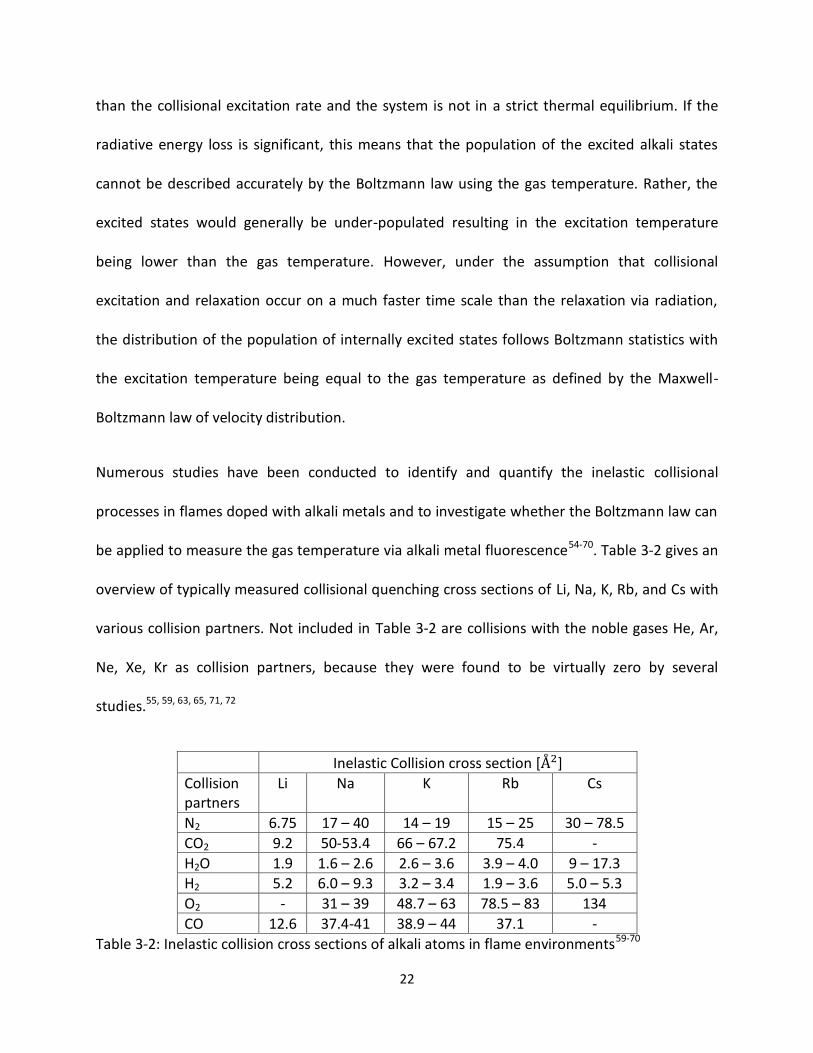
Numerous studies have been conducted to identify and quantify the inelastic collisional

processes in flames doped with alkali metals and to investigate whether the Boltzmann law can

be applied to measure the gas temperature via alkali metal fluorescence54-70. Table 3-2 gives an

overview of typically measured collisional quenching cross sections of Li, Na, K, Rb, and Cs with

various collision partners. Not included in Table 3-2 are collisions with the noble gases He, Ar,

Ne, Xe, Kr as collision partners, because they were found to be virtually zero by several

studies.55, 59, 63, 65, 71, 72

Inelastic Collision cross section [ ]

Collision partners

Li Na K Rb Cs

N2 6.75 17 – 40 14 – 19 15 – 25 30 – 78.5

CO2 9.2 50-53.4 66 – 67.2 75.4 -

H2O 1.9 1.6 – 2.6 2.6 – 3.6 3.9 – 4.0 9 – 17.3 H2 5.2 6.0 – 9.3 3.2 – 3.4 1.9 – 3.6 5.0 – 5.3

O2 - 31 – 39 48.7 – 63 78.5 – 83 134

CO 12.6 37.4-41 38.9 – 44 37.1 -

Table 3-2: Inelastic collision cross sections of alkali atoms in flame environments59-70

23

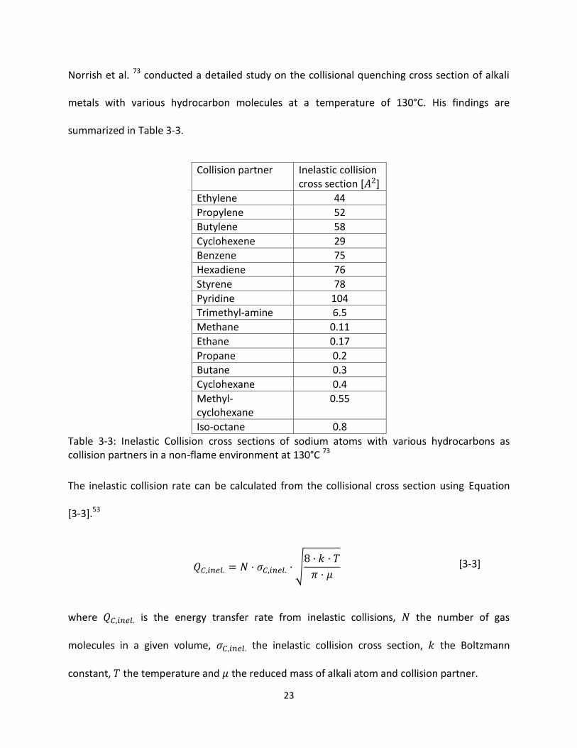
Norrish et al. 73 conducted a detailed study on the collisional quenching cross section of alkali

metals with various hydrocarbon molecules at a temperature of 130°C. His findings are

summarized in Table 3-3.

Collision partner Inelastic collision cross section [ ]

Ethylene 44

Propylene 52

Butylene 58

Cyclohexene 29 Benzene 75

Hexadiene 76

Styrene 78

Pyridine 104 Trimethyl-amine 6.5

Methane 0.11

Ethane 0.17

Propane 0.2 Butane 0.3

Cyclohexane 0.4

Methyl-cyclohexane

0.55

Iso-octane 0.8

Table 3-3: Inelastic Collision cross sections of sodium atoms with various hydrocarbons as collision partners in a non-flame environment at 130°C 73

The inelastic collision rate can be calculated from the collisional cross section using Equation

[3-3].53

√

[3-3]

where is the energy transfer rate from inelastic collisions, the number of gas

molecules in a given volume, the inelastic collision cross section, the Boltzmann

constant, the temperature and the reduced mass of alkali atom and collision partner.

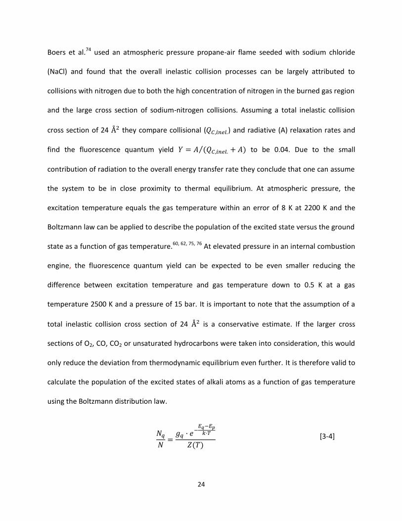
24

Boers et al.74 used an atmospheric pressure propane-air flame seeded with sodium chloride

(NaCl) and found that the overall inelastic collision processes can be largely attributed to

collisions with nitrogen due to both the high concentration of nitrogen in the burned gas region

and the large cross section of sodium-nitrogen collisions. Assuming a total inelastic collision

cross section of 24 they compare collisional ( ) and radiative (A) relaxation rates and

find the fluorescence quantum yield ( )⁄ to be 0.04. Due to the small

contribution of radiation to the overall energy transfer rate they conclude that one can assume

the system to be in close proximity to thermal equilibrium. At atmospheric pressure, the

excitation temperature equals the gas temperature within an error of 8 K at 2200 K and the

Boltzmann law can be applied to describe the population of the excited state versus the ground

state as a function of gas temperature.60, 62, 75, 76 At elevated pressure in an internal combustion

engine, the fluorescence quantum yield can be expected to be even smaller reducing the

difference between excitation temperature and gas temperature down to 0.5 K at a gas

temperature 2500 K and a pressure of 15 bar. It is important to note that the assumption of a

total inelastic collision cross section of 24 is a conservative estimate. If the larger cross

sections of O2, CO, CO2 or unsaturated hydrocarbons were taken into consideration, this would

only reduce the deviation from thermodynamic equilibrium even further. It is therefore valid to

calculate the population of the excited states of alkali atoms as a function of gas temperature

using the Boltzmann distribution law.

( ) [3-4]

25

where is the ratio of atoms in the excited state q versus the total number of atoms. The

partition function can be approximated as ( ) in the temperature range of interest. The

number of spontaneous emission processes is directly proportional to the population of the

excited state. We can therefore expect an exponential dependence of fluorescence signal

strength on burned gas temperature as illustrated in Figure 3-2.

Figure 3-2: The temperature dependent population of the lowest lying excited state of alkali

metals can be calculated using the Boltzmann distribution law:

For reasons that will be discussed in greater detail in section 3.5, it is of great interest to look at

the temperature dependence of measured fluorescence intensity ratios of various alkali metals.

0.000

0.001

0.002

0.003

0.004

0.005

0.006

0.007

0.008

0.009

0.010

1700 1900 2100 2300 2500

Excite

d S

tate

Po

pu

latio

n

[-]

Temperature [K]

Na

Rb

K

Li

Cs

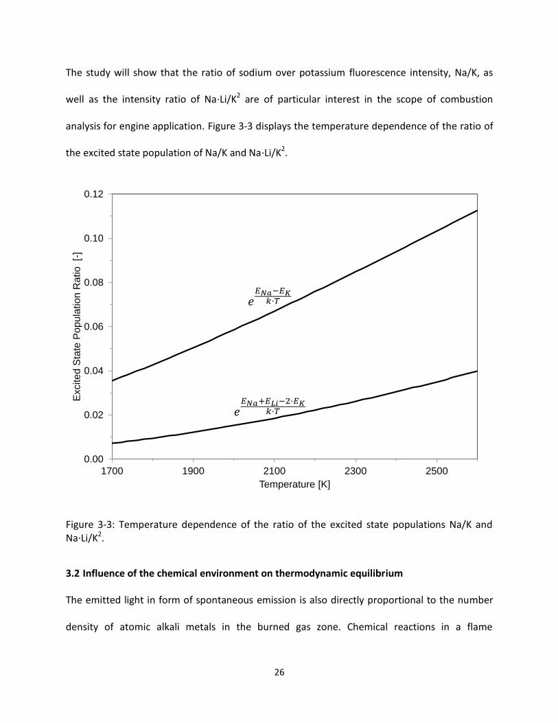
26

The study will show that the ratio of sodium over potassium fluorescence intensity, Na/K, as

well as the intensity ratio of Na·Li/K2 are of particular interest in the scope of combustion

analysis for engine application. Figure 3-3 displays the temperature dependence of the ratio of

the excited state population of Na/K and Na·Li/K2.

Figure 3-3: Temperature dependence of the ratio of the excited state populations Na/K and Na·Li/K2.

3.2 Influence of the chemical environment on thermodynamic equilibrium

The emitted light in form of spontaneous emission is also directly proportional to the number

density of atomic alkali metals in the burned gas zone. Chemical reactions in a flame

0.00

0.02

0.04

0.06

0.08

0.10

0.12

1700 1900 2100 2300 2500

Excite

d S

tate

Po

pu

latio

n R

atio

[-

]

Temperature [K]

27

environment affect the alkali atoms and in part convert them into their oxidation products,

which are predominantly the hydroxides. When the alkali atom is bound in a molecule, the

electronic wave function of the outer electron is changed and no more light can be emitted at

the wavelength of the atomic transition. It is therefore necessary to take chemical reactions

into consideration when computing the fraction of alkali metals that are left in elemental form

in the burned gas region at any given point during the combustion cycle.

Some studies have been conducted on the alkali reaction mechanism and kinetics in flames.

Glarborg et al. 77 investigated the reaction mechanism and formation of alkali sulfates in flames.

While their focus was set on the formation of sulfates, they provide reaction pathways and

kinetics data for the Na/O/H subsystem. Kaskan78 discusses likely reaction pathways for alkali in

H2/O2/N2 flames doped with sodium and potassium chloride and state that the formation of the

oxidation products occurs on a time scale fast enough to assume chemical equilibrium between

the elemental alkali and the oxidation product. This finding is backed by studies done by

Bulewicz et al.79 and James et al.80, who investigate the formation of hydrogen radicals via the

reaction of lithium with water to produce lithium hydroxide and atomic hydrogen in a fuel rich

H2/O2/N2 flame. While Kaskan78 finds the three body reaction of alkali with oxygen to be

dominant over the reaction of alkali with water, it should be noted that his calculations on

thermodynamic equilibrium used estimated data for the bond strength of Na-OH and Na-O of

90 and 80 kcal/mol, respectively. More recent data published by Hynes et al.81 provide a value

of 78.9±2.0 kcal/mol for the Na-OH bond and 60.3±4.0 kcal/mol for the Na-O bond. Hynes

et al.81 thoroughly investigated further thermodynamic properties of alkali hydroxide, oxide and

dioxide in various lean H2/O2/N2 flame environments between 1650 – 2400 K. They found the

28

hydroxide to be the dominant product species containing more than 99% of all bound alkali and

the alkali oxide and dioxide to only constitute a small fraction of the alkali product species.

Hynes et al.81 also proposed a reaction mechanism that produces results in close agreement to

their experimentally determined species concentration. They discuss previous work on alkali

reaction mechanisms and kinetics and address some large discrepancies in reaction rate

constants among the publications cited. It must be noted that these reaction mechanisms were

typically developed for H2/O2/N2 flames and Jensen et al.82 outline the typically large

uncertainties on the obtained values for the reaction rates. To the author’s knowledge no such

reaction mechanisms have been developed for the use in internal combustion engines running

on gasoline-like hydrocarbon fuel. Reliable modeling of alkali reaction kinetics in an engine

requires more chemical kinetics data.

Fortunately it is reasonable to assume thermodynamic equilibrium in the high temperature,

high pressure burned gas regions of internal combustion engines, based upon observations in

flames made by Hynes et al.81, Bulewicz et al.79, James et al.80 and Kaskan 78 on the rapid

equilibration in the burned gas region.

Thermodynamic properties such as enthalpy of formation and specific heat as a function of

temperature are given in Gurvich et al.83, 84, Chase85, as well as the database of the NIST

Chemistry WebBook2. Table 3-4 shows the enthalpy values for the most relevant alkali species.

29

[kJ/mol]

( )

[kJ/mol]

( ) ( )

[kJ/mol]

( ) ( )

[kJ/mol]

Li 159.3 ± 1.02, 85 35.382 336.0

-526.4 LiOH -234.3 ± 6.32

(-229.0 ± 5.0)83 92.9685

Li+ 685.7285 35.3885

Na 107.3 ± 0.72, 85 35.342 246.8

-502.0 NaOH -197.8 ± 12.62, 85

(-191 ± 8)83 93.683

Na+ 609.3485 35.3885

K 89.0 ± 0.42, 85 35.232 262.7

-425.0 KOH -232.6 ± 12.62, 85

(-232 ± 3)84 93.92, 85

K+ 514.0185 35.3885

Rb 80.9 ± 0.82, 85 35.142 (260.1)

-409.2 RbOH -

(-238.0 ± 5.0)84 -

(approx.93.9)84

Rb+ 490.132 35.382

Cs 76.5 ± 1.085 35.5085 277.1

-381.9 CsOH -259.4 ± 12.6

85

(-256.0 ± 5.0)84 94.28

85

Cs+ 458.4085 35.3885

Table 3-4: Thermodynamic properties of gas-phase alkali metals, ions and hydroxides. The difference on the total enthalpy of atom - hydroxide and atom - ion reflects the likeliness of hydroxide and ion formation, with lower values meaning that the equilibrium is shifted more strongly toward the atomic state.

The mean values provided by the NIST database2 and Chase et al.85 are used here with the

software Chemkin-Pro X64 Version 15101 to calculate thermodynamic equilibria in the burned

gas region of an internal combustion engine as a function of temperature, pressure and

equivalence ratio using iso-octane fuel. Other alkali species considered in the calculations are:

A-, AO, AO-, AH and A2, where the letter A represents all alkali elements. These species were

found to be of negligible importance in this study and are therefore not discussed in greater

detail.

30

The calculated fractions of atomic Li, Na, K, Rb and Cs and the ratios of atomic Na/K and

Na·Li/K2 are plotted in Figure 3-4 and Figure 3-5 as a function of temperature, equivalence ratio

and pressure. The chemical equilibria of all alkali elements depend strongly on temperature,

equivalence ratio and pressure (P). The atomic Na/K ratio shows a strong dependence on

temperature, equivalence ratio and pressure, while the Na·Li/K2 atom ratio depends on

temperature but is almost independent of equivalence ratio and pressure.

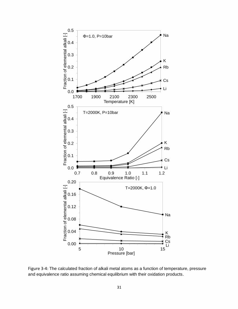
31

Figure 3-4: The calculated fraction of alkali metal atoms as a function of temperature, pressure

and equivalence ratio assuming chemical equilibrium with their oxidation products.

0.00

0.04

0.08

0.12

0.16

0.20

5 10 15

Fra

ctio

n o

f e

lem

en

tal a

lka

li [-

]

Pressure [bar]

0.0

0.1

0.2

0.3

0.4

0.5

0.7 0.8 0.9 1.0 1.1 1.2

Fra

ctio

n o

f ele

men

tal alk

ali

[-]

Equivalence Ratio [-]

0.0

0.1

0.2

0.3

0.4

0.5

1700 1900 2100 2300 2500

Fra

ctio

n o

f ele

men

tal alk

ali

[-]

Temperature [K]

Li

K

Rb

Cs

Na

Li

K

Rb

Cs

Na

Φ=1.0, P=10bar

T=2000K, P=10bar

T=2000K, Φ=1.0

Li

KRbCs

Na

32

Figure 3-5: The ratios of atomic Na/K and Na·Li/K2 show a strong dependence on temperature. While the Na/K ratio is also strongly affected by the equivalence ratio and to a lesser extent by the pressure, the quantity Na·Li/K2 is nearly independent of equivalence ratio and pressure.

Uncertainty in the literature data on the enthalpy of formation of the hydroxides is the primary

source of uncertainty in the calculation of the chemical equilibrium. Figure 3-6 and Figure 3-7

illustrate this effect on the ratios of atomic Na/K and Na·Li/K2 when the enthalpies of formation

of the lithium, sodium and potassium hydroxides are varied over the full range of uncertainty

(Hf,Li ±6.3 kJ/mol, Hf,Na and Hf,K ±12.6 kJ/mol). Using the value -210.4 kJ/mol for the sodium

hydroxide and -220.0 kJ/mol for potassium hydroxide almost entirely removes any atomic Na/K

0.04

0.06

0.08

0.10

0.12

0.14

0.16

0.18

0.20

0.22

1700 1900 2100 2300 2500

Fra

ction o

f ato

mic

Na·L

i/K

2

Temperature [K]

0.04

0.06

0.08

0.10

0.12

0.14

0.16

0.18

0.20

1700 1900 2100 2300 2500

Fra

ction o

f ato

mic

Na·L

i/K

2

Temperature [K]

1.5

2.0

2.5

3.0

3.5

4.0

1700 1900 2100 2300 2500

Fra

ction o

f ato

mic

Na/K

[-]

Temperature [K]

1.5

2.0

2.5

3.0

3.5

4.0

1700 1900 2100 2300 2500

Fra

ction o

f ato

mic

Na/K

[-]

Temperature [K]

P=10bar Φ=1.0

Φ=1.0P=10bar

Φ=0.8Φ=1.0Φ=1.2

P=5barP=10barP=15bar

33

ratio dependence on equivalence ratio and pressure, whereas the values -185.2 kJ/mol and -

245.2 kJ/mol for sodium hydroxide and potassium hydroxide, respectively, would result in a

significantly larger equivalence ratio and pressure dependence as well as altered temperature

dependence. Similarly the dependence of atomic Na·Li/K2 ratio on equivalence ratio, pressure

and temperature is significantly affected by the values chosen for the heats of formation of the

alkali hydroxides. In this study the mean values for the hydroxides will be used. The atomic

Na·Li/K2 ratio is nearly independent of equivalence ratio and pressure when using the mean

values for the heats of formation, which is an important observation for the subsequent

fluorescence image analysis. Overall, uncertainty in the heat of formation of the hydroxides is

the dominant cause of uncertainty for the subsequent model calculations.

34

Figure 3-6: The chemical equilibrium of atomic Na/K and Na·Li/K2 for three combinations of enthalpies of formation as a function of temperature and a constant pressure of 10 bar and for equivalence ratios of Φ=0.8 and Φ=1.2. The values for the enthalpies of formation were selected as the mean and the two extreme values of the reported uncertainties in Table 3-4.

Hf,NaOH=-185.2, Hf,KOH=-245.2 kJ/mol



0

4

8

12

16

20

24

1700 1900 2100 2300 2500

Fra

ction o

f ato

mic

Na/K

[-]

Temperature [K]

0.0

0.2

0.4

0.6

0.8

1.0

1.2

1700 1900 2100 2300 2500

Fra

ction o

f ato

mic

Na·L

i/K

2

Temperature [K]

P=10bar

P=10bar

Φ=0.8

Φ=1.2

Φ=0.8Φ=1.2

Data points for

Φ=0.8 and

Φ=1.2 nearly

identical

Data points for

Φ=0.8 and

Φ=1.2 nearly

identical

35

Figure 3-7: The chemical equilibrium of atomic Na/K and Na·Li/K2 is plotted for three combinations of enthalpies of formation as a function of temperature and a constant equivalence ratio of 1.0 and for pressures of P=5bar and P=15bar. The values for the enthalpies of formation were selected as the mean and the two extreme values of the reported uncertainties in Table 3-4.

0.0

0.2

0.4

0.6

0.8

1.0

1.2

1700 1900 2100 2300 2500

Fra

ction o

f ato

mic

Na·L

i/K

2

Temperature [K]

0

4

8

12

16

20

24

1700 1900 2100 2300 2500

Fra

ction o

f ato

mic

Na/K

[-]

Temperature [K]




Φ=1.0

Φ=1.0

P=5bar

P=15bar

P=5barP=15bar

Data points for

P=bar and

P=15bar nearly

identical

Data points for

P=5bar and

P=15bar nearly

identical

36

3.3 Assessment of self-absorption and line broadening of alkali fluorescence

3.3.1 Beer-Lambert law

Due to the presence of ground state alkali atoms in the burned gas region, some of the emitted

light can get re-absorbed by another ground state atom. Because collisional energy transfer is

dominant, there is little chance that the absorbed photon will get re-emitted. In good

approximation it is valid to consider all light that gets re-absorbed to be lost. The observed

intensity of the fluorescence is therefore influenced by the magnitude of self-absorption.

The Beer-Lambert law allows for calculating the fraction of the absorbed light.86

∫ ∫ ∫

( )

∫

[3-5]

where is the fraction of light being absorbed, is the emitted intensity of light, the

transmitted intensity of light, the frequency of light, the spectral distribution of light

energy, ( ) the spectral absorptivity, the number density of absorbing atoms and the

thickness of the burned gas region. In the case of self-absorption, the spectral profile of the

light emitting atom is identical to the absorption spectrum of the absorbing atom as long as

temperature and pressure remain unchanged. This requirement in combination with the

assumption of uniform distribution of alkali atoms in the burned gas volume, limit the accurate

computation of self-absorption to homogeneous engine conditions. In this case, can be

expressed by:

37

( ) [3-6]

where is a constant and ( ) the spectral emission and absorption profile whose integral is

normalized to one. Equation [3-5] can be written as:

∫ ∫ ( )

( ( ) )

[3-7]

The absorptivity can be expressed as:53

( ) ( ) [3-8]

where is the oscillator strength of the transition between the excited state and the

ground state . ( ) is determined by ways of natural line broadening, collision and Doppler

broadening and the latter two are strongly affected by temperature and pressure and are

dominant over natural line broadening in the engine environment.

3.3.2 Natural line broadening

The transition spectrum of electronic transitions in atoms is not infinitesimally narrow even

without any influence from external sources. This is due to Heisenberg’s uncertainty principle in

combination with the fact that the radiative life time of the excited state is finite.53

[3-9]

38

where is the energy uncertainty and the radiative lifetime of the quantum eigenstate.

The lifetime of the quantum state is finite resulting in a non-zero energy uncertainty, which

corresponds to an uncertainty in the transition frequency53

(

) [3-10]

where is the naturally broadened line width in frequency space. For the case of

transitioning the atom down into its ground state and approximating the life time of the ground

state as infinite, Equation [3-10] can be simplified to53

[3-11]

3.3.3 Collision line broadening

Line broadening due to atomic or molecular collisions in the gas phase can be subdivided into

inelastic and elastic collision broadening. Inelastic collisions cause a change in internal energy of

the atom, whereas elastic collisions are defined as collisions that leave the atom in the same

quantum state or merely transition it to another quantum state within the degenerate

subspace. Both types of collisions contribute to line broadening, with the cross sections for

elastic collisions often exceeding the inelastic cross sections by one order of magnitude or

more. A variety of literature sources53, 87-91 have conducted experimental measurements of

effective (elastic + inelastic) collision cross sections and the reported values show a spread of a

factor of more than two. Hofmann et al.89 provide a very reasonable explanation for this spread

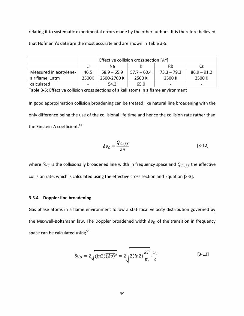
39

relating it to systematic experimental errors made by the other authors. It is therefore believed

that Hofmann’s data are the most accurate and are shown in Table 3-5.

Effective collision cross section [ ]

Li Na K Rb Cs Measured in acetylene-air flame, 1atm

46.5 2500K

58.9 – 65.9 2500-2760 K

57.7 – 60.4 2500 K

73.3 – 79.3 2500 K

86.9 – 91.2 2500 K

calculated - 54.3 65.0 - -

Table 3-5: Effective collision cross sections of alkali atoms in a flame environment

In good approximation collision broadening can be treated like natural line broadening with the

only difference being the use of the collisional life time and hence the collision rate rather than

the Einstein-A coefficient.53

[3-12]

where is the collisionally broadened line width in frequency space and the effective

collision rate, which is calculated using the effective cross section and Equation [3-3].

3.3.4 Doppler line broadening

Gas phase atoms in a flame environment follow a statistical velocity distribution governed by

the Maxwell-Boltzmann law. The Doppler broadened width of the transition in frequency

space can be calculated using53

√( )( )̅̅ ̅̅ ̅̅ √ ( )

[3-13]

40

3.3.5 Combination of line broadening effects and calculation of self-absorption

Natural broadening and collision broadening both follow a Lorentzian line shape. It is generally

valid to assume the natural and collision broadening effects to be mutually independent,

because they are caused by independent physical effects. Therefore these two broadening

effects can be combined to calculate the total Lorentzian line width by simply adding the

individual line widths.53

[3-14]

Doppler broadening does not follow a Lorentzian line shape and cannot be assumed to be

independent from Lorentzian broadening. It is, however, a valid simplification to treat both

effects as independent, because the error introduced by this assumption is small in the central

part of the profile. Using this simplification, the combined Voigt line width can be

calculated as derived in Alkemade et al.53

√

( ) ( ) [3-15]

The combined spectral Voigt profile is described by Alkemade et al.53 as:

( )

√

√

( )

∫

( ( )

)

(( ) ( )

)

[3-16]

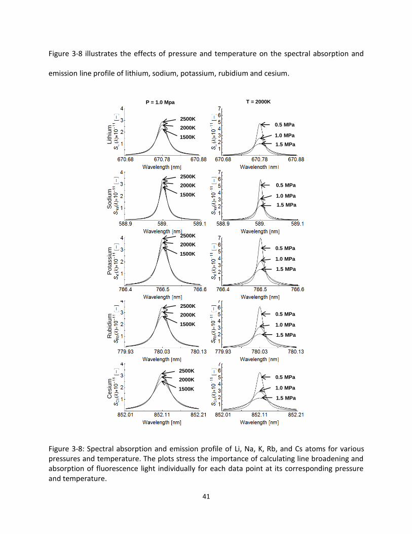
41

Figure 3-8 illustrates the effects of pressure and temperature on the spectral absorption and

emission line profile of lithium, sodium, potassium, rubidium and cesium.

Figure 3-8: Spectral absorption and emission profile of Li, Na, K, Rb, and Cs atoms for various pressures and temperature. The plots stress the importance of calculating line broadening and absorption of fluorescence light individually for each data point at its corresponding pressure and temperature.

0.5 MPa

1.0 MPa

1.5 MPa

2500K

2000K

1500K

P = 1.0 Mpa T = 2000K

2500K

2000K

1500K

2500K

2000K

1500K

2500K

2000K

1500K

2500K

2000K

1500K

0.5 MPa

1.0 MPa

1.5 MPa

0.5 MPa

1.0 MPa

1.5 MPa

0.5 MPa

1.0 MPa

1.5 MPa

0.5 MPa

1.0 MPa

1.5 MPa

Lithiu

mS

odiu

mP

ota

ssiu

mR

ubid

ium

Cesiu

m

42

The effect of absorption can now be calculated using Equation [3-7] if the number density of

ground state alkali atoms and the absorption path length are known. The number density can

be calculated using Equation [3-17]. It is necessary to know the concentration of alkali elements

in the fuel additive and the amount of fuel injected per engine cycle. The calculation of the

chemical equilibrium yields the mole fraction of alkali in elemental form in the burned gas

region. It is valid for this calculation to assume all alkali atoms to be in their electronic ground

state, since the excited state population is less than 1% in the temperature range of interest as

shown in Figure 3-2.

[3-17]

with the number density of alkali elements in the burned gas zone, the fraction of

elemental alkali in the burned gas region from the chemical equilibrium calculation in section

3.2, the mole fraction of alkali elements in the fuel, the mass of fuel injected per

engine cycle, the molecular mass of the fuel, the Avogadro constant and

the cylinder volume of the engine.

The cylinder volume of the engine in this study with the piston at bottom dead center

position is 500 cm3. The piston stroke of the engine used in this study is 8.5 cm, and the

distance between piston bowl and cylinder head at top dead center position is estimated as 1.5

cm. The total absorption length is therefore approximated as 10 cm with the piston in bottom

dead center position. It is important to note that the absorption length as well as the number

density will both change as a function of crank angle position, but the product of is

43

independent of crank angle position. Appendix A shows the processing macro to automate the

computation of absorption. The software used was ‘Wolfram Mathematica version 8.0.1.0

64bit’.

Figure 3-9 shows the fraction of transmitted fluorescence light of the various alkali species over

a range of temperatures, pressures and atomic mole fractions assuming 8.8 mg of fuel injected

per cycle. The transmission of the fluorescence light of all alkali metals is strongly affected by

temperature, pressure and mole fraction. While an exponential mole fraction dependence is

expected from the Beer-Lambert law in Equation [3-7], the temperature and pressure

dependence originates from pressure and temperature dependent line broadening. The ratio of

transmitted sodium over potassium intensity is hardly affected by pressure, temperature, and

mole fraction, whereas the Na·Li/K2 transmission ratio does depend on pressure and mole

fraction, but is nearly independent of temperature as shown in Figure 3-10.

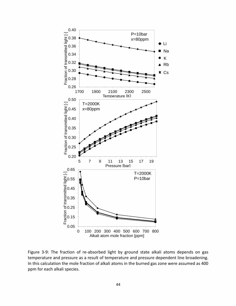
44

Figure 3-9: The fraction of re-absorbed light by ground state alkali atoms depends on gas temperature and pressure as a result of temperature and pressure dependent line broadening. In this calculation the mole fraction of alkali atoms in the burned gas zone were assumed as 400 ppm for each alkali species.

0.26

0.28

0.30

0.32

0.34

0.36

0.38

0.40

1700 1900 2100 2300 2500

Fra

ctio

n o

f tr

an

sm

itte

d lig

ht

[-]

Temperature [K]

0.20

0.25

0.30

0.35

0.40

0.45

0.50

5 7 9 11 13 15 17 19

Fra

ctio

n o

f tr

an

sm

itte

d lig

ht

[-]

Pressure [bar]

0.05

0.15

0.25

0.35

0.45

0.55

0.65

0 100 200 300 400 500 600 700 800

Fra

ctio

n o

f tr

an

sm

itte

d lig

ht

[-]

Alkali atom mole fraction [ppm]

Li

Na

K

Rb

Cs

P=10bar

x=80ppm

T=2000K

x=80ppm

T=2000K

P=10bar

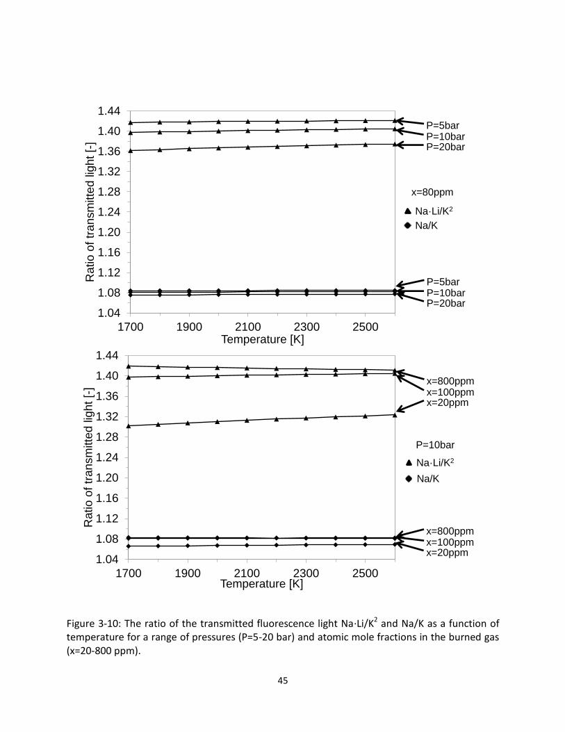
45

Figure 3-10: The ratio of the transmitted fluorescence light Na·Li/K2 and Na/K as a function of temperature for a range of pressures (P=5-20 bar) and atomic mole fractions in the burned gas (x=20-800 ppm).

1.04

1.08

1.12

1.16

1.20

1.24

1.28

1.32

1.36

1.40

1.44

1700 1900 2100 2300 2500

Ratio o

f tr

ansm

itte

d lig

ht

[-]

Temperature [K]

1.04

1.08

1.12

1.16

1.20

1.24

1.28

1.32

1.36

1.40

1.44

1700 1900 2100 2300 2500

Ratio o

f tr

ansm

itte

d lig

ht

[-]

Temperature [K]

Na·Li/K2

Na/K



x=800ppmx=100ppmx=20ppm

x=800ppmx=100ppmx=20ppm

Na·Li/K2

Na/K

x=80ppm

P=10bar

46

3.4 Other factors that influence alkali metal fluorescence intensity

Alkali metal fluorescence originates from the entire burned gas volume. The camera sees a two-

dimensional projection of the burned gas volume with the fluorescence integrated along the

camera’s line of sight. This makes the recorded intensity dependent on the thickness of the

burned gas cloud.

In addition, the alkali elements are bound to a larger organic complex and mixed into the fuel.

Before fluorescence light can be emitted by the alkali elements, the additives need to combust

releasing the alkali elements into the burned gas. This makes the overall fluorescence intensity

dependent on the burned fuel mass fraction.

Fortunately the effects of line-of-sight integration and burned fuel mass fraction affect the

fluorescence of all alkali metals in the same way. Recording the fluorescence of two or more

alkali metals simultaneously and ratioing the recorded fluorescence intensities can therefore

eliminate this effect. It is important to note that the various chemical and physical parameters

discussed above affect each alkali element differently, and therefore the fluorescence intensity

ratios of any two elements will still depend on temperature and equivalence ratio.

3.5 Selection of suitable alkali metals as fuel dopants

A thorough analysis was carried out to select the three most promising alkali elements for this

study. Sodium was selected due its thermodynamic equilibrium most strongly favoring the

atomic state, which promises good fluorescence signals under a wide range of temperatures

and equivalence ratios. Ionization was calculated to be negligible under the observed

47

temperature range of up to 2700 K. Its emission near 589.0 and 589.6 nm is close to the

sensitivity peak of the camera and both emission lines can be captured simultaneously with a

spectrally narrow bandpass filter. The only downside is that the excited state energy of sodium

is the highest of all alkali elements resulting in the lowest excited state population over the

entire temperature range.

Potassium and rubidium are expected to behave very similarly in the flame with regards to

temperature and equivalence ratio dependence due to the very small difference in excited

state energy and almost identical thermodynamic properties. Only one of the two elements can

be selected since the K/Rb fluorescence ratio would not be sensitive to temperature or

equivalence ratio changes. The thermodynamic equilibrium of potassium and rubidium and

their respective hydroxides favor the atomic state more than in the case of cesium or lithium.

Their excited state energies are lower than the lithium’s and only slightly higher than in the

case of cesium. Ionization of both elements becomes relevant at elevated temperature above

2500 K and must be accounted for. Potassium is preferred over rubidium because its emission

lines at 766.5 and 769.9 nm are much closer than the 780.0 and 794.8 nm lines of rubidium and

can therefore be captured simultaneous with a narrower bandpass filter.

Cesium differs from the selected sodium and potassium in both its temperature dependence

and thermodynamic equilibrium. Its excited state population is the highest of all alkali elements

over the entire temperature range due to its low excited state energy. Cesium is most prone to

ionization, but this would only become important at the high end of the observed temperature

range, where the fluorescence signal is strong due to the high excited state population and the

48

thermodynamic equilibrium favoring the atomic state. Fluorescence intensity loss due to high

temperature ionization is therefore no experimental concern and can be accounted for

quantitatively. Although the emission lines of cesium at 852.1 and 894.4 nm are separated too

far to capture them both simultaneously with a narrow bandpass filter, the camera chip

sensitivity is still sufficient for the stronger line at 852.1 nm. Although the camera is more

sensitive to the lithium emission lines near 670.8 nm and a narrow bandpass filter can capture

both lithium lines, the thermodynamic equilibrium of lithium is most strongly shifted toward

the hydroxide. Particularly at low temperature and lean operating conditions, the cesium signal

is expected to be stronger than the lithium fluorescence. However, no commercially available,

cesium containing, organic fuel additive could be identified and therefore lithium was used as

the third alkali element in this study rather than the preferred cesium.

3.6 Model prediction of alkali fluorescence intensity in the engine

With the dependences of alkali fluorescence intensity on the collisional energy exchange

environment, the chemical equilibrium and the effect of self-absorption understood, the

expected measured fluorescence intensities of lithium, sodium and potassium and the intensity

ratios of Na/Li, Li/K, Na/K and Na·Li/K2 can be predicted. The mole fractions of lithium, sodium

and potassium in the fuel used in the subsequent experiments were 5340ppm, 322ppm and

284ppm, respectively, and these values were used in the following calculations. The three

combustion parameters affecting the fluorescence intensity are temperature, pressure and

equivalence ratio. Appendix B contains a flow chart illustrating the sequence of computation

steps to build a database of expected fluorescence intensities and intensity ratios as a function

49

of pressure, temperature and equivalence ratio. Figure 3-11 shows the dependence of the

Na/Li, Li/K, Na/K and Na·Li/K2 fluorescence intensity ratios on temperature and equivalence

ratio for a constant pressure of 10 bar. The Na/Li, Li/K and Na/K fluorescence intensity ratios

each show strong dependences on temperature. The signal ratios are most strongly affected by

equivalence ratio between Φ=0.9 to Φ=1.1 and at temperatures less than 2100K. While the

equivalence ratio dependences continue in a less sensitive way in the fuel rich regime, the

fluorescence intensity ratios are nearly independent of equivalence ratio between Φ=0.5 to

Φ=0.9. It is apparent that the equivalence ratio dependence of the predicted Li/K fluorescence

intensity ratio is nearly the inverse of the Na/K ratio. The product of both ratios to form the

quantity Na·Li/K2 is therefore nearly independent of equivalence ratio but shows a strong

dependence on temperature. Na·Li/K2 shows only a small equivalence ratio dependence in the

rich regime and at high temperature.

Figure 3-12 illustrates the dependence of the Na/Li, Li/K, Na/K and Na·Li/K2 fluorescence

intensity ratios on pressure at a constant equivalence ratio of Φ=1.0. While the Na/Li, Li/K and

Na/K ratios are significantly affected by pressure, it is observed that the pressure dependence

of the Na/K and Li/K ratios are opposite but nearly equal in magnitude. The Na·Li/K2

fluorescence intensity ratio remains therefore nearly unaffected by pressure over the entire

temperature range of interest.

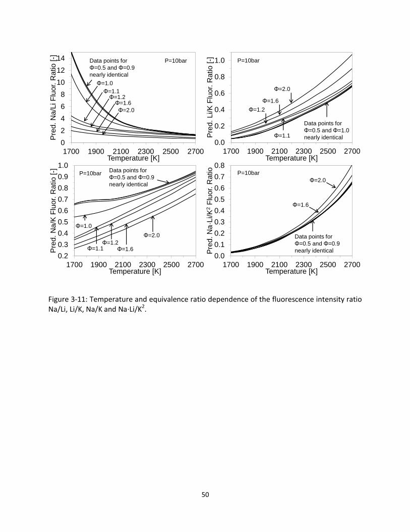
50

Figure 3-11: Temperature and equivalence ratio dependence of the fluorescence intensity ratio Na/Li, Li/K, Na/K and Na·Li/K2.

0.0

0.1

0.2

0.3

0.4

0.5

0.6

0.7

0.8

1700 1900 2100 2300 2500 2700

Pre

d. N

a·L

i/K

2F

luor. R

atio

Temperature [K]

0.2

0.3

0.4

0.5

0.6

0.7

0.8

0.9

1.0

1700 1900 2100 2300 2500 2700

Pre

d. N

a/K

Flu

or. R

atio [

-]

Temperature [K]

0.0

0.2

0.4

0.6

0.8

1.0

1700 1900 2100 2300 2500 2700

Pre

d. Li/K

Flu

or. R

atio [

-]

Temperature [K]

0

2

4

6

8

10

12

14

1700 1900 2100 2300 2500 2700

Pre

d. N

a/L

i F

luor. R

atio [

-]

Temperature [K]

P=10barData points for

Φ=0.5 and Φ=0.9

nearly identical

Φ=1.0

Φ=1.1Φ=1.2Φ=1.6

Φ=2.0

Data points for

Φ=0.5 and Φ=0.9

nearly identical

Data points for

Φ=0.5 and Φ=1.0

nearly identicalΦ=1.1

Φ=1.2

Φ=1.6

Φ=2.0

P=10bar

P=10bar P=10bar

Φ=1.0

Φ=1.1Φ=1.2

Φ=1.6

Φ=2.0 Data points for

Φ=0.5 and Φ=0.9

nearly identical

Φ=1.6

Φ=2.0

51

Figure 3-12: Temperature and pressure dependence of the fluorescence intensity ratio Na/Li, Li/K, Na/K and Na·Li/K2.

While any of the two-component ratios could be used for temperature measurements in

homogeneous combustion environments, where both cylinder pressure and equivalence ratio

are known, the combination of three alkali components to form the Na·Li/K2 fluorescence ratio

is preferred due to its independence from pressure and equivalence ratio. In stratified

combustion environments, where both temperature and local equivalence ratio are unknown,

the Na·Li/K2 fluorescence intensity ratio can be used as a direct marker for burned gas

temperature independently of cylinder pressure and equivalence ratio. It is the preferred

choice for temperature measurements in both homogeneous and stratified combustion

1

3

5

7

9

11

13

15

1700 1900 2100 2300 2500 2700

Pre

d. N

a/L

i F

luor. R

atio [-]

Temperature [K]

0.0

0.1

0.2

0.3

0.4

0.5

0.6

0.7

0.8

1700 1900 2100 2300 2500 2700

Pre

d. Li/K

Flu

or. R

atio [

-]

Temperature [K]

0.4

0.5

0.6

0.7

0.8

0.9

1.0

1700 1900 2100 2300 2500 2700

Pre

d.

Na

/K F

luo

r. R

atio

[-]

Temperature [K]

0.0

0.1

0.2

0.3

0.4

0.5

0.6

0.7

1700 1900 2100 2300 2500 2700

Pre

d. N

a·L

i/K

2F

luor. R

atio

Temperature [K]

Φ=1.0

P=30bar

P=20bar

P=10bar

P=4bar

P=30bar

P=20bar

P=10bar

P=4barΦ=1.0

Φ=1.0Φ=1.0 P=30bar

P=20bar

P=10bar

P=4bar

Data points for

P=4bar to P=30bar

nearly identical

52

environments. When the temperature is measured using the Na·Li/K2 fluorescence intensity

ratio, any of the two-component ratios Na/Li, Li/K or Na/K can be used for the simultaneous

measurement of local equivalence ratio. The Na/K signal ratio is expected to yield the highest

signal to noise ratio due to the very faint fluorescence intensity of lithium in cold and lean

zones. Appendix C illustrates how the database of computed alkali fluorescence intensity ratios

can be used to post-processes the recorded fluorescence intensities and obtain burned gas

temperature and equivalence ratio.

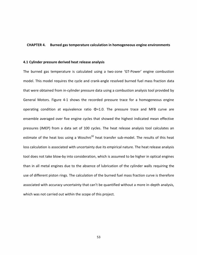
53

CHAPTER 4. Burned gas temperature calculation in homogeneous engine environments

4.1 Cylinder pressure derived heat release analysis

The burned gas temperature is calculated using a two-zone ‘GT-Power’ engine combustion

model. This model requires the cycle and crank-angle resolved burned fuel mass fraction data

that were obtained from in-cylinder pressure data using a combustion analysis tool provided by

General Motors. Figure 4-1 shows the recorded pressure trace for a homogeneous engine

operating condition at equivalence ratio Φ=1.0. The pressure trace and MFB curve are

ensemble averaged over five engine cycles that showed the highest indicated mean effective

pressures (IMEP) from a data set of 100 cycles. The heat release analysis tool calculates an

estimate of the heat loss using a Woschni92 heat transfer sub-model. The results of this heat

loss calculation is associated with uncertainty due its empirical nature. The heat release analysis

tool does not take blow-by into consideration, which is assumed to be higher in optical engines

than in all metal engines due to the absence of lubrication of the cylinder walls requiring the

use of different piston rings. The calculation of the burned fuel mass fraction curve is therefore

associated with accuracy uncertainty that can’t be quantified without a more in-depth analysis,

which was not carried out within the scope of this project.

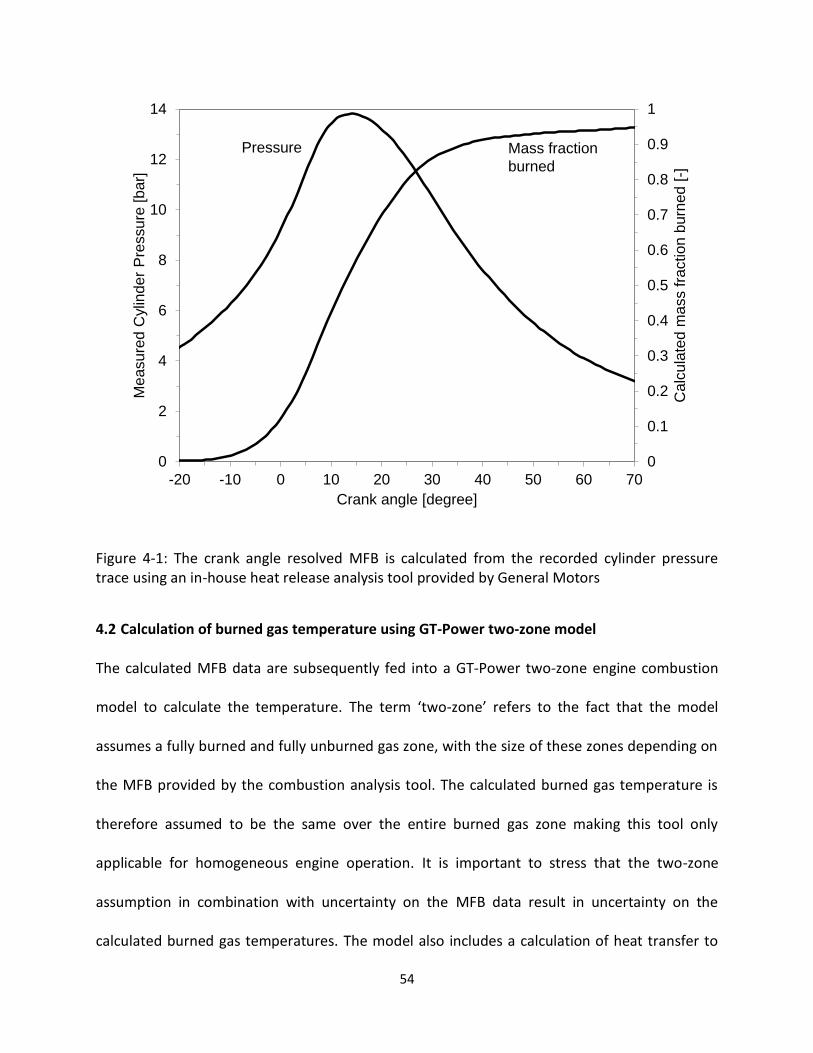
54

Figure 4-1: The crank angle resolved MFB is calculated from the recorded cylinder pressure trace using an in-house heat release analysis tool provided by General Motors

4.2 Calculation of burned gas temperature using GT-Power two-zone model

The calculated MFB data are subsequently fed into a GT-Power two-zone engine combustion

model to calculate the temperature. The term ‘two-zone’ refers to the fact that the model

assumes a fully burned and fully unburned gas zone, with the size of these zones depending on

the MFB provided by the combustion analysis tool. The calculated burned gas temperature is

therefore assumed to be the same over the entire burned gas zone making this tool only

applicable for homogeneous engine operation. It is important to stress that the two-zone

assumption in combination with uncertainty on the MFB data result in uncertainty on the

calculated burned gas temperatures. The model also includes a calculation of heat transfer to

0

0.1

0.2

0.3

0.4

0.5

0.6

0.7

0.8

0.9

1

0

2

4

6

8

10

12

14

-20 -10 0 10 20 30 40 50 60 70

Calc

ula

ted m

ass fra

ction b

urn

ed [

-]

Measu

red

Cylin

der

Pre

ssure

[b

ar]

Crank angle [degree]

Pressure Mass fraction

burned

55

the walls of the combustion chamber and provides various heat transfer sub-models named

‘WoschniGT’, ‘WoschniSwirl’, ‘WoschniHuber’ and ‘Hohenberg’. All these heat transfer models

are empirical in nature and were developed for certain combustion chamber geometries and

operating conditions. Both the combustion chamber geometry of the engine used in this study

as well as the operating conditions are different from what these models were originally

calibrated for. In addition, the optical engine used in this study is expected to have significantly

different wall heat capacity and convection properties due to the quartz inserts in the piston

bowl and cylinder head. The two-zone model also uses a ‘Convective Heat Transfer Multiplier’

(CHTM), which should typically be set to a value between 1.0 and 1.4 according to the GT-

Power help files without a more detailed description of it. GT-Power also requires input data for

the wall temperatures of cylinder head, piston and cylinder walls. The engine used in this study

was not instrumented to measure these temperatures and the values must be estimated. The

discussed assumptions and simplifications inherent to this model introduce accuracy

uncertainty to the calculated burned gas temperature, which can’t be quantified in detail.

However, a comparison of the calculated temperatures by varying these parameters can offer

an estimate of the overall uncertainty. Figure 4-2 shows calculated burned gas temperatures

using the ‘WoschniSwirl’ heat transfer with a convective heat transfer multiplier of 1.35 and

425K, 500K and 550K as the cylinder wall, cylinder head and piston temperature, respectively.

The heat release analysis tool calculates small but non-zero values for the burned fuel mass

fraction very early in the cycle. This is unrealistic, because the spark timing was set to 32° bTDC

and no heat release can occur before that. However, it results in the calculation of a burned gas

temperature early in the cycle if no artificial threshold is set as displayed in Figure 4-2. Setting a

56

threshold of 1% burned fuel mass fraction in the GT-Power model still results in an initial

temperature spike that seems unrealistic. A threshold of 2% MFB produces a calculated

temperature curve without the initial temperature spike that seems intuitively more realistic.

This finding leads to the suspicion that the calculated temperatures early in the cycle are less

accurate due to the fact that the burned gas zone is small in size and small inaccuracies in the

calculated heat transfer result in large inaccuracies in the calculated burned zone temperature.

Figure 4-2: Calculated burned gas temperatures using 'WoschniSwirl' heat transfer model and a convective heat transfer multiplier of 1.35. Small values of MFB result in a unrealistic calculated burned gas temperature early in the cycle. Setting an artificial threshold of 1% MFB for the temperature calculation still results in an unphysical initial spike, while a 2% MFB threshold produces an intuitively reasonable temperature curve. In all three cases the calculated burned gas temperatures are nearly identical after TDC.

1700

1800

1900

2000

2100

2200

2300

2400

2500

2600

2700

-120 -100 -80 -60 -40 -20 0 20 40 60 80

Calc

ula

ted b

urn

ed

gas t

em

pe

ratu

re [

K]

Crank Angle aTDC [degree]

No threshold

1% MFB

threshold

2% MFB

threshold

57

In Figure 4-3 a comparison of the calculated burned gas temperatures using different heat

transfer sub-models is shown. In all cases the convective heat transfer multiplier was set to

1.35, the cylinder wall, cylinder head and piston temperature to 425K, 500K and 550K,

respectively, and a threshold of 2% MFB was used. The ‘WoschniHuber’ model still produces

and initial temperature spike despite the MFB threshold. The calculated burned gas

temperatures show a discrepancy of up to 75K indicating that the heat transfer sub-models

have a large impact on the resulting calculated temperature. It is important to keep in mind the

empirical nature of the various models. It is not possible to determine which of these models is

the most accurate and it is nearly arbitrary which of these sub-models to choose. The

‘WoschniSwirl’ model was chosen for all subsequent burned gas temperature calculations in

this study, considering that a high swirl motion was present in the combustion chamber of the

engine because of the deactivation of one intake valve and to be consistent with the fact that a

Woschni heat transfer model is also used in the heat release analysis tool to calculate the crank

angle resolved mass fraction of burned fuel.

58

Figure 4-3: The caluated burned gas temperatures depend on the heat transfer sub-model selection in GT-Power. The heat transfer sub-model selection can account for a deviation of the burned gas temperature of up to 75K. Although there is no quantitative justification for either one of the sub-models, the ‘WoschniSwirl’ model was used for all temperature calculations in this study.

An analysis of the effect of the convective heat transfer multiplier on the calculated burned gas

temperature is shown in Figure 4-4. As expected, a lower convective heat transfer multiplier

results in overall higher burned gas temperatures and higher values of the multiplier

consequently produce lower burned gas temperatures. It is assumed that a high swirl motion

will result in an overall higher convective heat transfer. Given the range of 1.0 – 1.4 provided by

the GT-Power help file, a value of 1.35 was chose for all subsequent temperature calculations in

1700

1800

1900

2000

2100

2200

2300

2400

2500

2600

-20 -10 0 10 20 30 40 50 60 70 80

Calc

ula

ted b

urn

ed g

as t

em

pera

ture

[K

]


WoschniHuber

Hohenberg

WoschniSwirl

WoschniGT

59

this study. However, it must be stressed that this decision is based on assumptions and results

in additional accuracy uncertainty that can’t be quantified in detail.

Figure 4-4: The calculated burned gas temperature is strongly affected by the value of the convective heat transfer multiplier (CHTM) in GT-Power. As expected, a lower multiplier values result in a higher calculated burned gas temperature. The value 1.35 was chosen for all temperature calculations in this study in agreement with the GT-Power help files and accounting for the high swirl motion in the combustion chamber due to the deactivation of one intake valve.

Aside from burned gas temperatures, the GT-Power two-zone model also calculates the

cylinder pressure. This calculated cylinder pressure can be compared to the measured cylinder

pressure to estimate the overall accuracy of the two-zone model calculation. Measured and

calculated pressure traces are displayed in Figure 4-5. It is interesting to observe that the

calculated pressure traces show only little deviation among the various heat transfer models

1700

1800

1900

2000

2100

2200

2300

2400

2500

2600

2700

-20 -10 0 10 20 30 40 50 60 70 80

Calc

ula

ted b

urn

ed

gas t

em

pe

ratu

re [

K]


CHTM=2.00

CHTM=0.00

CHTM=1.35

CHTM=1.00

60

used in the calculations. However, all calculations show a significant deviation from the

measured pressure trace of up to 1 bar early in the cycle near TDC. This may in part be

explained qualitatively by the assumed uncertainty of the heat release analysis tool. If this tool

calculated too low early MFB data due to inaccuracy of the heat transfer submodel, the

calculated cylinder pressure in GT-Power would be lower than the measured pressure. It is

therefore concluded that the accuracy of the burned gas temperature calculation is not very

reliable early in the cycle, but more accurate between 30-70° aTDC, since measured and

calculated pressure traces agree well in this range.

Figure 4-5: Selection of various heat transfer sub-models has little influence on the calculated cylinder pressure. The calculated pressures all differ up to 1 bar from the measured cylinder pressure early in the cycle and are in good agreement with the measurement after 30° aTDC.

3

4

5

6

7

8

9

10

11

12

13

14

-20 -10 0 10 20 30 40 50 60 70

Cylin

der

Pre

ssure

[b

ar]

Crank Anlge aTDC [degree]

measured

calculated using various heat

transfer sub-models

61

Figure 4-6 shows a comparison of calculated cylinder pressures using the WoschniSwirl model

and varying the wall temperatures by ±100 K. The measured and calculated pressure traces

agree best early in the cycle before the onset of combustion using 425K, 500K and 550K as the

cylinder wall, cylinder head and piston temperature, respectively. A higher wall temperature

produces an overall higher calculated cylinder pressure and a lower wall temperature results in

lower cylinder pressures as expected. Consequently, 425K, 500K and 550K as the cylinder wall,

cylinder head and piston temperature, respectively, were used in all burned gas temperature

calculations during this study. It must be stressed, however, that different combinations of

cylinder head, cylinder wall and piston temperature could produce a very similar calculated

cylinder pressure. In addition, the surface temperature of the metal and the quartz inserts may

differ due to the different heat capacity and hat conduction properties of these materials. This

can’t be reflected in the GT-Power simulation. The surface temperatures will also vary

depending on the operating condition and the duration of engine operation before the start of

the data acquisition. Consequently, an unknown accuracy uncertainty is introduced by

estimating these values.

62

Figure 4-6: The cylinder wall, cylinder head and piston temperature were set to 325K, 400K and 450K (T1), 425K, 500K, 550K (T2) and 525K, 600K, 650K (T3) in the GT-Power calculation and the resulting calculated cylinder pressure is compared to the measured cylinder pressure trace.

Another mode of performing a two-zone temperature calculation is to feed the measured,

crank-angle resolved pressure trace into the model instead of the MFB data calculated by the

heat release analysis tool. This mode shall be called ‘measured cylinder pressure mode’ (CP

mode) for the sake of this discussion, while the previous mode of feeding the mass fraction of

burned fuel shall be named ‘mass fraction burned mode’ (MFB mode). In a first step of the

measured cylinder pressure mode GT-Power will use the pressure data to derive the MFB curve

and use this subsequently in a forward run to calculate the simulated cylinder pressure and the

burned gas temperature. Figure 4-7a shows that in this mode the simulated cylinder pressure

3

4

5

6

7

8

9

10

11

12

13

14

-20 -10 0 10 20 30 40 50 60 70

Cylin

der

Pre

ssure

[bar]


measured

T3T2

T1

63

matches the measured pressure trace more closely than in Figure 4-5 and Figure 4-6. However,

GT-Power does not calculate the internal residual burned gas fraction based on the flow

dynamics through the intake, cylinder and exhaust manifold as it does in the MFB mode. While

it is possible to input an estimated value to the measured cylinder pressure mode, it is

important to know the residual burned gas fraction precisely because of its strong effect on the

calculated burned gas temperature. To illustrate this, Figure 4-7b shows the calculated burned

gas temperatures for three cases of the measured cylinder pressure mode with estimated

residual burned gas fractions of 0%, 12.4% and 20% as well as the calculated burned gas

temperature of the MFB mode, where the residual burned gas fraction was computed as 12.4%.

Figure 4-7: (a) Running the GT-Power two-zone model in cylinder pressure (CP) mode produces a simulated cylinder pressure trace that is generally in better agreement with the measured pressure trace than in the mass fraction burned (MFB) mode. However, the results depend on the residual burned gas fraction (Res), which has to be input manually in CP mode while it is calculated as 12.4% in MFB mode. (b) The calculated burned gas temperature depends strongly on the residual burned gas fraction. The observation that the calculate temperature in CP mode with 12.4% residual fraction is slightly lower than in MFB mode, although the simulated cylinder pressure is higher.

3

5

7

9

11

13

15

-20 0 20 40 60 80

Cylin

de

r P

ressu

re [b

ar]


1600

1800

2000

2200

2400

2600

2800

-20 0 20 40 60 80

Ca

lcu

late

d b

urn

ed

ga

s

tem

pera

ture

[K

]


measured

MFB mode,

Res 12.4%

CP mode, Res 0%

CP mode, Res 12.4%

CP mode, Res 20%

MFB mode,

Res 12.4%

CP mode,

Res 0%

CP mode,

Res 12.4%

CP mode,

Res 20%

a) b)

64

While it is important to match the measured cylinder pressure closely to have confidence in the

burned gas temperature calculation, this analysis shows that knowledge of the residual burned

gas fraction is at least of equal importance. For this reason it was decided to use the MFB mode

of GT-Power in this study knowing that either way of performing the temperature calculation is

associated with uncertainty. Due to the various, unquantifiable factors that are due to

simplifications and empirical assumptions in both the heat release analysis tool and the two-

zone model, an overall uncertainty of T ±100K is estimated for the calculated burned gas

temperature.

65

CHAPTER 5. Alkali metal fluorescence imaging in the engine

5.1 Experimental setup and operating conditions

Measurements in a homogeneously operated optical engine were conducted to obtain a range

of validation data for the model that describes lithium, sodium and potassium fluorescence

under engine conditions. Unfortunately, cylinder pressure, temperature and equivalence ratio

cannot be varied individually in the engine, so the model validation is limited to a few

homogeneous engine operating conditions at different equivalence ratios with the cylinder

pressure and temperature changing simultaneously throughout the engine cycle. Subsequently

various stratified-charge operating conditions were investigated to illustrate the potential of

this diagnostic tool for experimental engine research. A direct injected, 500 cm3 single-cylinder

gasoline engine with optical access through a piston window was used and run at 2000 rpm at

various equivalence ratios with 8.8 ±0.2 mg of fuel injected in each cycle at 290 degrees before

combustion top dead center. The cylinder pressure was measured with crank-angle resolution

using a pressure transducer (Kistler 6125A). A throttle plate in one of the two intake ports was

used to generate a high swirl motion in the combustion chamber. The air intake system allows

for diluting the air with additional amounts of nitrogen to simulate the effects of exhaust gas

recirculation on engine combustion. The air/fuel ratio was obtained by metering intake air flow

with a critical orifice and the fuel using a Coriolis (Micro Motion Elite CMF010) mass flow meter,

via the oxygen and carbon balance of the emissions bench, as well as via an oxygen sensor in

66

the exhaust manifold. The air/fuel ratio obtained by the Coriolis meter was used in the

calculation, and the accuracy uncertainty of ±1.3% was determined by comparisons to the

emissions bench readings. The precision error of the Coriolis meter was determined as ±2.7%

via the comparison of measured fuel mass flow from multiple engine experiments with identical

injector pulse width. The total uncertainty of the measured equivalence ratio is therefore less

than ±3.0%. Iso-octane served as the fuel instead of commercial gasoline and was doped with

two alkali containing additives dissolved in heavy oil (75 cst). One of the additives contained a

combination of lithium carbonate, sodium carbonate and potassium nitrate. The manufacturer

(SPEX CertiPrep) specification of the lithium, sodium and potassium mass fractions in this

additive was 3500 ppm, 1000 ppm and 1500 ppm. An additional, lithium (5000 ppm) carbonate

containing fuel additive was used to enhance the lithium fluorescence intensity. 50ml of the

combined fuel additive and 15ml of the additional lithium fuel additive were mixed into one

liter of iso-octane. The mole fractions of lithium, sodium and potassium in the fuel were 5340

ppm, 322 ppm and 284 ppm, respectively.

Three CMOS high-speed cameras (Vision Research Phantom V7.1) were used to record the

fluorescence of lithium, sodium and potassium, respectively. The quantum efficiency of the

cameras reported by the manufacturer was 33%, 27% and 22% near 589nm, 671nm and

767nm, respectively.93 The optical path of the emitted lithium, sodium and potassium light from

the engine was split using two dichroic filters. The first dichroic filter (Edmund Optics NT43-962)

with 99% reflectivity near 589 nm, 40% reflectivity near 671 nm and 98% transmission near 767

nm was used to separate the potassium fluorescence from lithium and sodium fluorescence.

The second dichroic filter was custom designed by Rocky Mountain Instrument Co. with 94%

67

transmission at 589 nm and 99.5% reflectivity near 671 nm to split sodium and lithium

fluorescence. This arrangement allows the cameras to share an identical line of sight into the

combustion chamber to ensure good spatial overlap of the images. A schematic of the

experimental setup is shown in Figure 5-1.

Figure 5-1: Experimental setup for the simultaneous high-speed imaging of lithium, sodium and potassium fluorescence

Band-pass filters on each camera lens with center wavelength of 671.0 nm (FWHM 10 nm, 90%

peak transmission, 50mm diameter), 589.0 nm (FWHM 10 nm, 100% peak transmission, 50mm

diameter) and 766.5 nm (FWHM 10 nm, 50% peak transmission, 50mm diameter), respectively,

ensured that any soot or combustion luminosity other than alkali fluorescence did not interfere

Cylinder head

Piston with glass insert

Broadband mirror

670nm dichroic mirror

Li+Na+Ksignal

Na signal

K signal

Camera-2 with 671nm bandpass filter


Field of View

Intake side

Exhaust side

Spark plug


Li signal650nm dichroic mirror

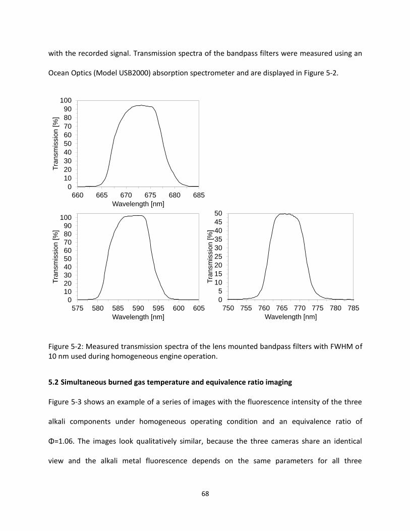
68

with the recorded signal. Transmission spectra of the bandpass filters were measured using an

Ocean Optics (Model USB2000) absorption spectrometer and are displayed in Figure 5-2.

Figure 5-2: Measured transmission spectra of the lens mounted bandpass filters with FWHM of 10 nm used during homogeneous engine operation.

5.2 Simultaneous burned gas temperature and equivalence ratio imaging

Figure 5-3 shows an example of a series of images with the fluorescence intensity of the three

alkali components under homogeneous operating condition and an equivalence ratio of

Φ=1.06. The images look qualitatively similar, because the three cameras share an identical

view and the alkali metal fluorescence depends on the same parameters for all three

0

5

10

15

20

25

30

35

40

45

50

750 755 760 765 770 775 780 785

Tra

nsm

issio

n [

%]

Wavelength [nm]

0

10

20

30

40

50

60

70

80

90

100

660 665 670 675 680 685

Tra

nsm

issio

n [

%]

Wavelength [nm]

0

10

20

30

40

50

60

70

80

90

100

575 580 585 590 595 600 605

Tra

nsm

issio

n [

%]

Wavelength [nm]

69

components. The fluorescence intensities, however, differ quantitatively in their dependence

on burned gas temperature, cylinder pressure and equivalence ratio. This becomes apparent in

Figure 5-4, where the ratios of the Na·Li/K2 and Na/K fluorescence intensities are illustrated

after the recorded images in Figure 5-3 were normalized by their respective camera exposure

time. The spatial and temporal intensity gradients of the fluorescence intensity ratio images are

much more homogeneous than in Figure 5-3, because the Na/K ratio only depends on burned

gas temperature, pressure and equivalence ratio and the Na·Li/K2 ratio is only temperature

dependent. Because the fuel was injected early in the cycle at 290° bTDC, neither temperature

nor equivalence ratio are expected to substantially differ spatially.

Figure 5-5 shows spatial profiles of the Li, Na, K, Na·Li/K2 and Na/K fluorescence images to

illustrate the spatial heterogeneities of the Li, Na and K fluorescence intensities. The profiles are

taken in vertical (from intake to exhaust side) direction immediately to the right of the spark

plug. The Li, Na and K fluorescence intensities show large spatial gradients due to their strong

dependence on the depth of the burned gas zone, which differs spatially due to the pent-roof

shaped cylinder head. While the spatially averaged fluorescence intensities can be compared to

the model predictions as a function of temperature, pressure and equivalence ratio, it is not

possible to utilize these signals directly for spatially resolved burned gas temperature

measurements in the engine. The fluorescence intensity ratios are nearly homogeneous,

because they only depend on temperature, pressure and equivalence ratio and neither of these

scalars is expected to differ substantially in space due to the nearly homogeneous engine

operating condition.

70

Figure 5-3: Simultaneously recorded sodium, lithium and potassium fluorescence of a single engine cycle under homogeneous operating conditions at an equivalence ratio of Φ=1.06. The images show strong temporal and spatial intensity gradients due to their dependence on mass fraction of burned fuel and depth of the burned gas zone.

Na Li K

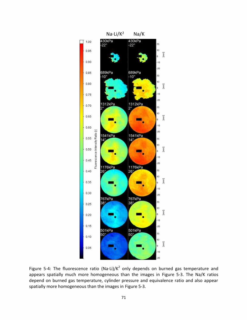
71

Figure 5-4: The fluorescence ratio (Na·Li)/K2 only depends on burned gas temperature and appears spatially much more homogeneous than the images in Figure 5-3. The Na/K ratios depend on burned gas temperature, cylinder pressure and equivalence ratio and also appear spatially more homogeneous than the images in Figure 5-3.

Na·Li/K2 Na/K

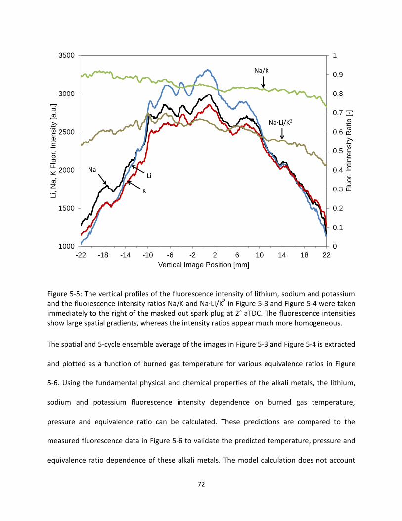
72

Figure 5-5: The vertical profiles of the fluorescence intensity of lithium, sodium and potassium and the fluorescence intensity ratios Na/K and Na·Li/K2 in Figure 5-3 and Figure 5-4 were taken immediately to the right of the masked out spark plug at 2° aTDC. The fluorescence intensities show large spatial gradients, whereas the intensity ratios appear much more homogeneous.

The spatial and 5-cycle ensemble average of the images in Figure 5-3 and Figure 5-4 is extracted

and plotted as a function of burned gas temperature for various equivalence ratios in Figure

5-6. Using the fundamental physical and chemical properties of the alkali metals, the lithium,

sodium and potassium fluorescence intensity dependence on burned gas temperature,

pressure and equivalence ratio can be calculated. These predictions are compared to the

measured fluorescence data in Figure 5-6 to validate the predicted temperature, pressure and

equivalence ratio dependence of these alkali metals. The model calculation does not account

0

0.1

0.2

0.3

0.4

0.5

0.6

0.7

0.8

0.9

1

1000

1500

2000

2500

3000

3500

-22 -18 -14 -10 -6 -2 2 6 10 14 18 22

Flu

or.

Intinte

nsity R

atio [

-]

Li, N

a, K

Flu

or.

Inte

nsity [

a.u

.]

Vertical Image Position [mm]

LiNa

K

Na/K

Na·Li/K2

73

for the solid angle of the camera lens, and therefore the calculated Li, Na, K deviates from the

measurement by a constant factor. The Na/K and Na·Li/K2 fluorescence intensity ratios are of

great interest in this study, because they are independent of the solid angle of the camera lens

as well as less dependent on mass fraction of burned fuel and depth of the burned gas volume.

The temperature and equivalence ratio dependences agree well with the measurement. The

quantity Na·Li/K2 shows a strong temperature dependence but is nearly independent of

equivalence ratio. It can therefore be used for burned gas temperature measurements in

stratified engine environments. The Na/K ratio can be used in combination with the Na·Li/K2

ratio to simultaneously calculate equivalence ratio and temperature from the recorded alkali

fluorescence. All data points were extracted late in the cycle after peak burned gas

temperature was reached, where combustion is nearly complete and the burned gas zone is

fully expanded.

It is important to note that the cylinder pressure changes throughout the cycle and for different

engine operating conditions. The apparent temperature and equivalence ratio dependences are

therefore partly caused by pressure dependences. Unfortunately it is difficult to vary burned

gas temperature, pressure and equivalence ratio independently in engine experiments.

Therefore, the model predictions were validated with the recorded fluorescence intensities and

intensity ratios for the few combinations of temperature, pressure and equivalence ratios that

were achieved in the experiments. The precision uncertainty in the recorded Na/K and Na·Li/K2

fluorescence intensity ratios is estimate via the standard deviation of the 5-cycle ensemble

average at crank angle 20° aTDC as ±0.007 and ±0.009, resulting in a 95% confidence interval of

±0.014 and ±0.018, respectively. The plotted data range covers the expansion stroke (12° - 70°

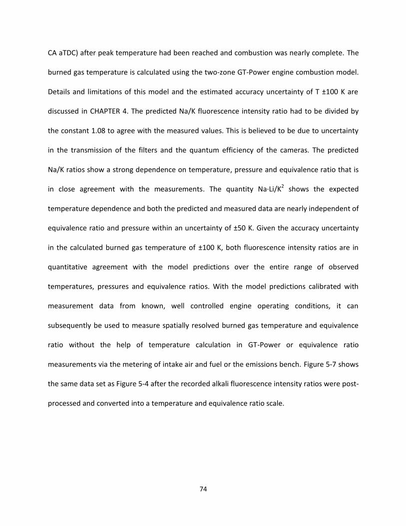
74

CA aTDC) after peak temperature had been reached and combustion was nearly complete. The

burned gas temperature is calculated using the two-zone GT-Power engine combustion model.

Details and limitations of this model and the estimated accuracy uncertainty of T ±100 K are

discussed in CHAPTER 4. The predicted Na/K fluorescence intensity ratio had to be divided by

the constant 1.08 to agree with the measured values. This is believed to be due to uncertainty

in the transmission of the filters and the quantum efficiency of the cameras. The predicted

Na/K ratios show a strong dependence on temperature, pressure and equivalence ratio that is

in close agreement with the measurements. The quantity Na·Li/K2 shows the expected

temperature dependence and both the predicted and measured data are nearly independent of

equivalence ratio and pressure within an uncertainty of ±50 K. Given the accuracy uncertainty

in the calculated burned gas temperature of ±100 K, both fluorescence intensity ratios are in

quantitative agreement with the model predictions over the entire range of observed

temperatures, pressures and equivalence ratios. With the model predictions calibrated with

measurement data from known, well controlled engine operating conditions, it can

subsequently be used to measure spatially resolved burned gas temperature and equivalence

ratio without the help of temperature calculation in GT-Power or equivalence ratio

measurements via the metering of intake air and fuel or the emissions bench. Figure 5-7 shows

the same data set as Figure 5-4 after the recorded alkali fluorescence intensity ratios were post-

processed and converted into a temperature and equivalence ratio scale.

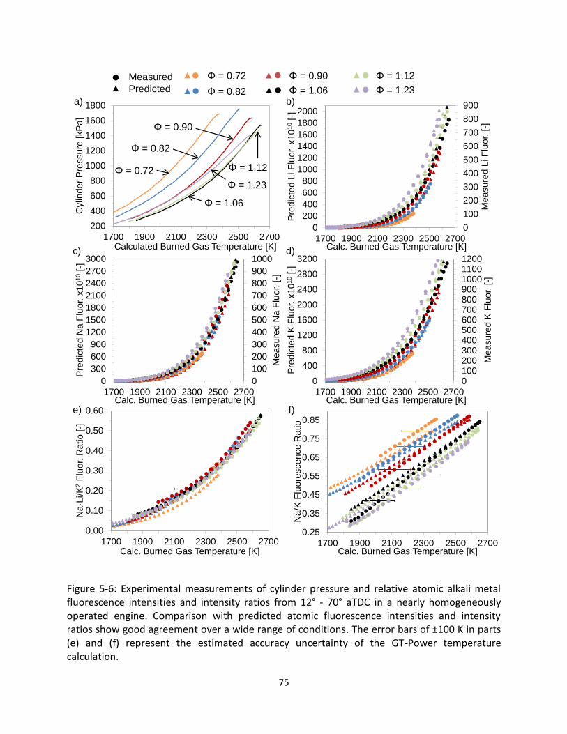
75

Figure 5-6: Experimental measurements of cylinder pressure and relative atomic alkali metal fluorescence intensities and intensity ratios from 12° - 70° aTDC in a nearly homogeneously operated engine. Comparison with predicted atomic fluorescence intensities and intensity ratios show good agreement over a wide range of conditions. The error bars of ±100 K in parts (e) and (f) represent the estimated accuracy uncertainty of the GT-Power temperature calculation.

0.25

0.35

0.45

0.55

0.65

0.75

0.85

1700 1900 2100 2300 2500 2700

Na

/K F

luo

resce

nce

Ra

tio

Calc. Burned Gas Temperature [K]

0.00

0.10

0.20

0.30

0.40

0.50

0.60

1700 1900 2100 2300 2500 2700

Na

·Li/K

2F

luo

r. R

atio

[-]


200

400

600

800

1000

1200

1400

1600

1800

1700 1900 2100 2300 2500 2700

Cylin

de

r P

ressu

re [

kP

a]

Calculated Burned Gas Temperature [K]

0100200300400500600700800900100011001200

0

400

800

1200

1600

2000

2400

2800

3200

1700 1900 2100 2300 2500 2700

Measure

d K

Flu

or. [-]

Pre

dic

ted K

Flu

or. x

10

10

[-]


0

100

200

300

400

500

600

700

800

900

1000

0

300

600

900

1200

1500

1800

2100

2400

2700

3000

1700 1900 2100 2300 2500 2700

Measure

d N

a F

luor. [

-]

Pre

dic

ted N

a F

luo

r. x

10

10

[-]


0

100

200

300

400

500

600

700

800

900

0

200

400

600

800

1000

1200

1400

1600

1800

2000

1700 1900 2100 2300 2500 2700

Measure

d L

i F

luor. [

-]

Pre

dic

ted L

i F

luo

r. x

10

10

[-]


a)

c)

Predicted

Measured Φ = 0.72

Φ = 0.82

Φ = 0.90

Φ = 1.06

Φ = 1.12

Φ = 1.23

d)

e) f)

b)

Φ = 0.72

Φ = 0.82

Φ = 0.90

Φ = 1.06

Φ = 1.12

Φ = 1.23

76

Figure 5-7: Simultaneous imaging of burned gas temperature and equivalence ratio after the recorded alkali fluorescence intensities were post-processed. The numbers in the top left corner of each image denote the measured cylinder pressure and crank angle position. The rectangular and circular black areas in the center of the images mask out the spark plug ground strap and a dust grain on one of the camera chips, respectively.

T TΦ Φ

≤0.9

77

It must be noted that the calibration curves from Figure 5-6 were generated for data points late

in the cycle where combustion was nearly complete, the burned gas zone was fully expanded

and the absorption path length was large. The equivalence ratio images early in the cycle and

around the perimeter of the burned gas zone in Figure 5-7 appear richer than expected, but

once the burned gas zone in Figure 5-7 has expanded further, the calculated local equivalence

ratios are in good agreement with the global equivalence ratio of Φ=1.06 measured by the

emissions bench and the fuel and air metering systems. The measured equivalence ratio late in

the cycle appears richer than expected. This is largely attributed to very low fluorescence

intensity at the low temperature late in the cycle, which decreases the signal to noise ratio of

the images. The images show some spatial stratification with the local equivalence ratio in the

center region being richer than in the outer regions of the piston bowl. The equivalence ratio is

also measured to be leaner at the bottom (exhaust) side of the piston bowl than at the top

(intake) side. This stratification was not expected due to the early injection of fuel at 290° bTDC,

but the spatial RMS of ±0.08 lies within the reported measurement uncertainty of ±10% of

previously used tools such as LIF23, which could explain why it has not been detected before.

The fluorescence based temperature measurement is compared to the GT-Power two-zone

temperature calculation in Figure 5-8. The measured data agree with the calculation within ±15

K between 10-70 °CA aTDC, where the burned gas zone is fully expanded and combustion is

nearly complete, but deviate by up to 90 K early in the combustion cycle at -10° aTDC. The

fluorescence based temperature measurement is therefore expected to very accurately capture

local temperature differences, but it is important to point out that the overall accuracy of the

absolute temperature values is coupled to the GT-Power accuracy uncertainty of ±100K.

78

The large temperature deviation early in the cycle, in combination with the equivalence ratio

being measured too rich, indicates that the burned gas temperature obtained from the alkali

fluorescence early in the cycle and around the perimeter of the burned gas zone is

systematically biased towards lower values.

Mainly two reasons could potentially explain the inaccuracy in these regions: (1) The burned

gas zone is not fully expanded in the direction of the cameras’ line of sight for small flame

kernels and near the outer regions of the burned gas zone, which impacts the magnitude of

self-absorption of the fluorescence intensity. However, the calculations that lead to

temperatures and equivalence ratios displayed in Figure 5-7 assumed a fully expanded burned

gas zone. (2) The assumption of a complete chemical equilibrium may not be valid for regions in

or near the flame front. Both effects will be included in a comprehensive discussion of

measurement uncertainties in section 5.3.

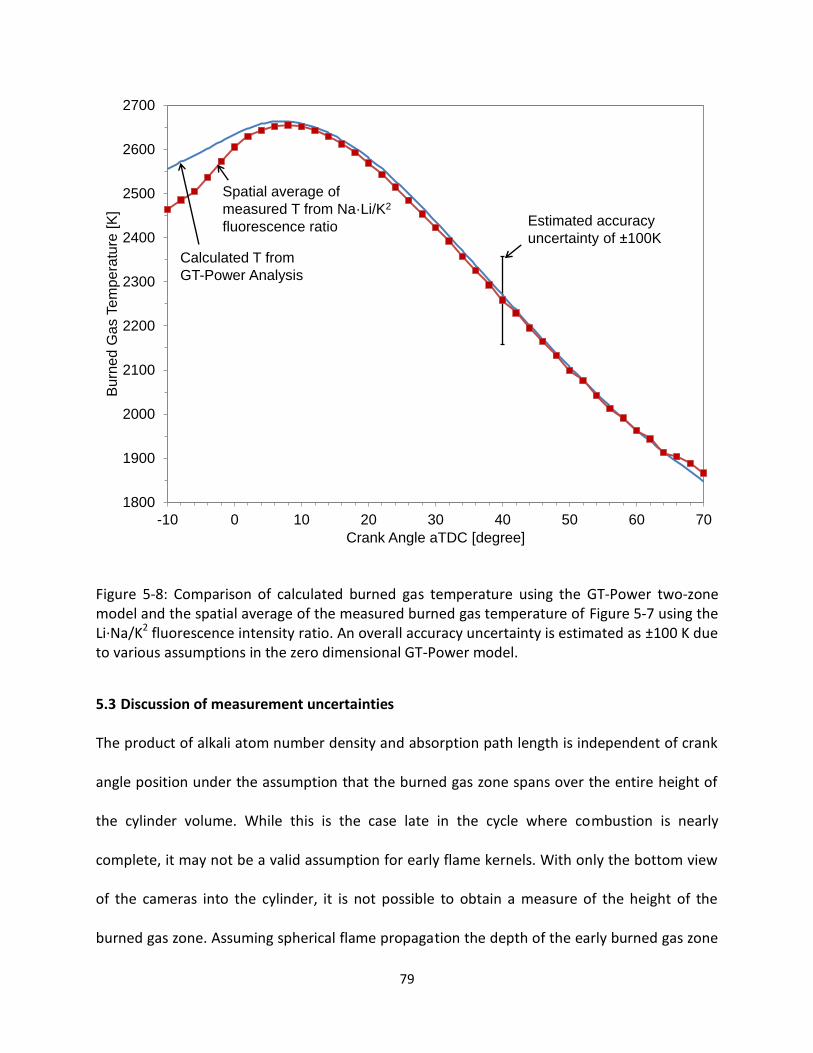
79

Figure 5-8: Comparison of calculated burned gas temperature using the GT-Power two-zone model and the spatial average of the measured burned gas temperature of Figure 5-7 using the Li·Na/K2 fluorescence intensity ratio. An overall accuracy uncertainty is estimated as ±100 K due to various assumptions in the zero dimensional GT-Power model.

5.3 Discussion of measurement uncertainties

The product of alkali atom number density and absorption path length is independent of crank

angle position under the assumption that the burned gas zone spans over the entire height of

the cylinder volume. While this is the case late in the cycle where combustion is nearly

complete, it may not be a valid assumption for early flame kernels. With only the bottom view

of the cameras into the cylinder, it is not possible to obtain a measure of the height of the

burned gas zone. Assuming spherical flame propagation the depth of the early burned gas zone

1800

1900

2000

2100

2200

2300

2400

2500

2600

2700

-10 0 10 20 30 40 50 60 70

Burn

ed G

as T

em

pera

ture

[K

]


Spatial average of

measured T from Na·Li/K2

fluorescence ratio

Calculated T from

GT-Power Analysis

Estimated accuracy

uncertainty of 100K

80

is nearly zero around its perimeter and radiation trapping should be negligible in this area. The

model was modified to assume no self-absorption and re-applied to the early flame images to

improve the accuracy of the temperature and equivalence ratio measurement. Figure 5-9

shows the calculated equivalence ratio at -10° aTDC for the same cycle as Figure 5-7, where the

two limiting cases of absorption paths lengths are compared. The equivalence ratio in part (a)

was calculated assuming the depths of the burned gas cloud being fully expanded, which is

most appropriate for the center region of the image. The spatially averaged burned gas

temperature was calculated as 2463 K, as shown in Figure 5-8. Part (b) assumes the complete

absence of absorption, which would be the limiting case for the perimeter of the burned gas

zone assuming spherical flame propagation. In the limit of the assumed absence of self-

absorption, the measured equivalence ratio is richer than in case (a) even around the perimeter

of the burned gas zone. The spatially averaged burned gas temperature for this case is 2375 K,

which deviates even stronger from the GT-Power calculation. The comparison shows that the

correct assumption of the depths of the burned gas zone is important for the imaging of early

flame kernels, but it does not explain the observed discrepancies in the measured burned gas

temperature and equivalence ratio.

81

Figure 5-9: The calculated equivalence ratio of an early flame kernel assuming that (a) the depth of the burned gas cloud is fully expanded and the absorption path length is maximum and (b) complete absence of absorption.

The calculated dependences of the fluorescence intensities on temperature, pressure and

equivalence ratio assume all combustion species to be in a state of total thermal equilibrium.

While this is nearly the case in the burned gas zone, where combustion is complete, it is not

necessarily a valid assumption near the flame front, which forms the perimeter of the early

flame kernel where the measured temperatures and equivalence ratios deviate substantially

from the known values. Previous studies have reported super-equilibrium concentrations of

hydroxyl (OH)94 and hydrogen (H) radicals79 that would affect the chemical balance between

alkali atoms and their hydroxides and lead to a deviation from the assumed chemical

equilibrium between the alkali atoms and their oxidation products. A potential solution to this

problem would be the inclusion of reaction kinetics in the model instead of the assumption of

≤0.90

a) b)

82

thermodynamic equilibrium. However, not enough information is available with regards to the

exact composition of the alkali metal fuel additives and their reaction pathways and reaction

rates in the flame. In addition, no alkali reaction mechanism is available for engine combustion

environments using iso-octane or gasoline-like fuels. The reaction mechanisms that were

developed in H2/O2/N2 flames differ largely in their reported reaction rate constants. It is

therefore currently not possible to include reaction kinetics into the model calculations to

improve the alkali fluorescence based temperature and equivalence ratio measurements in or

near the flame front.

Uncertainty is introduced by the assumption of a homogeneous burned gas temperature in the

combustion chamber, which is required for the two-zone GT-Power combustion model. Since

the lithium, sodium and potassium fluorescence intensities depend exponentially on burned gas

temperature, a thermal stratification along the cameras’ line of sight causes the integrated

fluorescence to correspond to a temperature higher than the calculated mean. This effect

would be less pronounced for the Na·Li/K2 and Na/K fluorescence ratios, because their

exponent in the Boltzmann term is much smaller, but still poses a limitation to the quantitative

application of this tool to stratified combustion environments.

Similarly, the integration of the recorded fluorescence intensity along the cameras’ line of sight

in a stratified combustion environment would generally bias the measured equivalence ratio

towards values that are richer than the line of sight average, because the fluorescence intensity

is generally higher in richer zones. Additionally, in cases where self-absorption of the alkali

fluorescence is significant, the temperature and equivalence ratio measurement will be biased

83

to areas closer to the cameras (in this study the piston top), because photons originating from

this region are more likely to escape the cylinder due to their shorter path length. Self-

absorption of the alkali fluorescence could be minimized to less than 2% of the emitted light

under most engine conditions, if the alkali mole fractions in the fuel were reduced by a factor of

approximately 500. This would reduce the recorded fluorescence intensity by a factor of

approximately 100 and necessitate the use of image intensifiers.

The assessment of the precision error of the temperature and equivalence ratio imaging in the

engine is complicated by the fact that combustion cycles are not truly repeatable. At a stable,

nearly stoichiometric engine operating condition, the temperature and equivalence ratio was

measured of 50 consecutive, individual cycles at crank angle 20° aTDC. The 50 cycles were

sorted by their IMEP, and the five cycles with the highest IMEP were selected. The coefficient of

variance (COV) of the IMEP of these five cycles was 0.008. Due to the almost identical engine

performance, it is assumed that the burned gas temperature is identical among these five

cycles. The standard deviation of the spatially averaged temperature and equivalence ratio

measurement was 9.2 K and 0.01, resulting in a 95% confidence interval of ±18K and ±0.02,

respectively.

The accuracy uncertainty of the temperature calculation in the zero dimensional GT-Power

model cannot be fully quantified because of the required estimation of various software

parameters that was discussed in section 4.2. However, systematic variations of the major

parameters influencing the burned gas temperature calculation in the engine lead to an

estimate of T ±100K in this study. The accuracy of the alkali fluorescence based temperature

84

measurement is therefore also limited to an uncertainty of ±100K, since the calculated

temperature from GT-Power is used for the calibration of the alkali fluorescence tool. To

improve the accuracy of the fluorescence imaging tool, a more reliable calibration methodology

would need to be identified. It is important to stress that any spatial or temporal temperature

differences observed with this tool are not affected by this, but the absolute temperature

values are affected by an estimated accuracy uncertainty of ±100K.

Accuracy uncertainty in the imaging of equivalence ratio is not affected by the uncertainty in

the calculated burned gas temperature, because the equivalence ratio obtained from the Na/K

fluorescence intensity ratio is calibrated using the calculated burned gas temperature of GT-

Power and the measured equivalence ratio obtained from the fuel and air metering system. The

calibration decoupled the accuracy of the equivalence ratio obtained from the alkali

fluorescence from the accuracy uncertainty of the burned gas temperature. Accuracy

uncertainty in the equivalence ratio calculated from the alkali fluorescence ratio Na/K is

introduced by the ±3.0% uncertainty in the equivalence ratio obtained from the fuel and air

metering system, which is used for the calibration of the fluorescence tool. This could be

improved by performing the calibration in a more controlled environment such as a premixed

flame burner. The equivalence ratio measurement via alkali fluorescence imaging generally has

the best sensitivity near stoichiometric equivalence ratio and low temperature, but generally no

sensitivity for Φ ≤ 0.9.

85

5.4 Mass fraction of burned fuel imaging using the spatially integrated sodium fluorescence

The integrated sodium fluorescence intensity depends on pressure, temperature, equivalence

ratio, absorption and mass fraction of burned fuel. Once the temperature and equivalence ratio

have been obtained through the Na·Li/K2 and Na/K fluorescence intensity ratios, the spatially

integrated sodium fluorescence intensity can be corrected for the effects of pressure,

temperature, equivalence ratio and self-absorption on the sodium fluorescence intensity using

model calculations. After the correction has been applied, the spatially integrated sodium

fluorescence intensity is expected to show linear dependence on MFB. With the current

experimental setup this correlation can only be performed early in the cycle before the burned

gas zone has spread beyond the field of view of the cameras. Sodium fluorescence images that

were ensemble averaged over five engine cycles in the range from -24° to -2° CA aTDC and MFB

0.005 to 0.163, respectively, are shown in Figure 5-10 for engine operation and equivalence

ratio Φ=1.06. The spark plug electrode is not masked out in the center of these images to

minimize error in the spatial integration of the fluorescence intensity. It must be noted,

however, that the spark plug ground strap itself covers the view into the spark plug gap

between ground strap and electrode.

86

Figure 5-10: Sodium fluorescence images of the early flame kernel in a homogeneous, stoichiometric engine operation. The numbers in the left and right upper corners of the images denote crank angle position aTDC and MFB, respectively. No mask was applied to cover the spark plug electrode to minimize error in the subsequent spatial integration of the sodium signal. However, the presence of the spark plug electrode introduces uncertainty especially for small flame kernels.

87

The spatially integrated sodium fluorescence is extracted from the images and plotted in Figure

5-11a as a function of calculated MFB for equivalence ratios ranging between 0.72 and 1.23.

The sodium fluorescence intensities differ largely at any given MFB depending on the engine

operating condition. This is expected because the recorded sodium fluorescence intensity also

depends on the burned gas temperature, pressure, equivalence ratio and self-absorption,

which differ for each operating condition. The integrated fluorescence signal is subsequently

corrected for its dependence on temperature, pressure, equivalence ratio and absorption and

the corrected fluorescence intensities are plotted in Figure 5-11b. The data show a linear

correlation with MFB and nearly collapse onto the same curve for the various engine operating

conditions. This shows that the spatially integrated sodium fluorescence intensity can be used

to measure MFB within an experimental uncertainty of ±0.02 provided the burned gas

temperature and equivalence ratio are known from the three component fluorescence

intensity ratios.

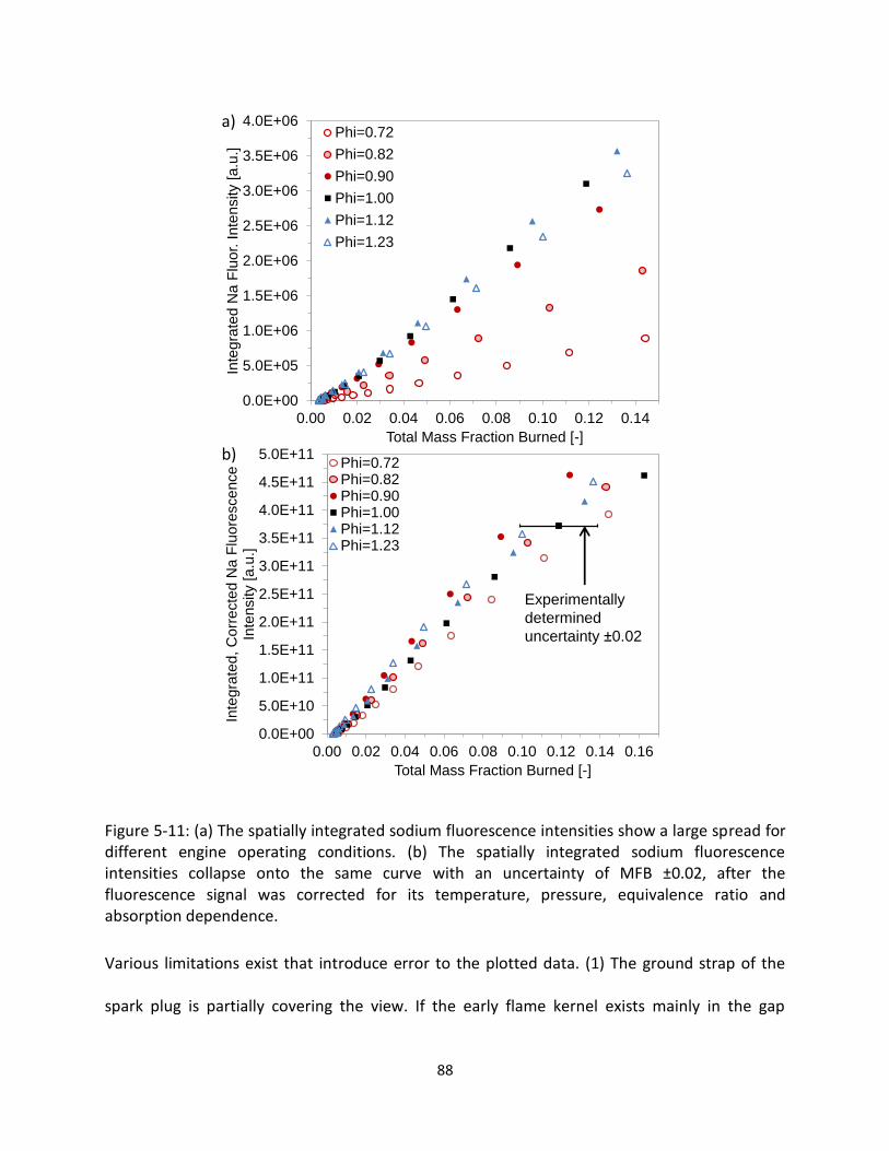
88

Figure 5-11: (a) The spatially integrated sodium fluorescence intensities show a large spread for different engine operating conditions. (b) The spatially integrated sodium fluorescence intensities collapse onto the same curve with an uncertainty of MFB ±0.02, after the fluorescence signal was corrected for its temperature, pressure, equivalence ratio and absorption dependence.

Various limitations exist that introduce error to the plotted data. (1) The ground strap of the

spark plug is partially covering the view. If the early flame kernel exists mainly in the gap

0.0E+00

5.0E+10

1.0E+11

1.5E+11

2.0E+11

2.5E+11

3.0E+11

3.5E+11

4.0E+11

4.5E+11

5.0E+11

0.00 0.02 0.04 0.06 0.08 0.10 0.12 0.14 0.16

Inte

gra

ted

, C

orr

ecte

d N

a F

luore

sce

nce

Inte

nsity [a.u

.]

Total Mass Fraction Burned [-]

Phi=0.72Phi=0.82Phi=0.90Phi=1.00Phi=1.12Phi=1.23

0.0E+00

5.0E+05

1.0E+06

1.5E+06

2.0E+06

2.5E+06

3.0E+06

3.5E+06

4.0E+06

0.00 0.02 0.04 0.06 0.08 0.10 0.12 0.14

Inte

gra

ted

Na

Flu

or.

In

ten

sity [

a.u

.]

Total Mass Fraction Burned [-]

Phi=0.72

Phi=0.82

Phi=0.90

Phi=1.00

Phi=1.12

Phi=1.23

a)

b)

Experimentally

determined

uncertainty 0.02

89

between ground strap and spark plug electrode, the measured sodium signal for early crank

angles may not be visible to the camera. (2) The spark is occasionally carried with the in-

cylinder air flow and the arc becomes visible to the camera for early crank angles despite the

bandpass filters. This will cause interference with the recorded sodium signal, since the camera

cannot distinguish between the two. The use of filters with even narrower spectral bandwidths

could help avoid interference from the spark arc. (3) At the very onset of combustion the

relative uncertainty in the MFB values calculated by the heat release analysis tool is highest.

The MFB is calculated as 0.005 even before the start of combustion. (4) The sodium

fluorescence was corrected for self-absorption using the burned zone diameter as the

absorption length assuming spherical flame propagation. However, this will still introduce error

in the outer regions of the burned gas zone, where the burned zone thickness is smaller.

However, with the current view it is not possible to know the depth of the burned gas zone

accurately at each point. Imaging from multiple directions would yield more accurate

knowledge of the thickness of the burned gas zone.

90

CHAPTER 6. Application of alkali fluorescence imaging in stratified engine environments

6.1 Individual cycle analysis in a spray-guided engine operation with high cyclic variations

Figure 6-1 shows a comparison of a well burning (Figure 6-1a, IMEP 151 kPa) and poorly burning

(Figure 6-1b, IMEP 70 kPa) engine cycle during spray-guided, stratified engine operating. The

injector used was an 8-hole injector with 60° spray angle and a length over diameter (L/D) ratio

of the injector holes of 2.0. The engine speed was 800 rpm and the intake air was diluted with

32% nitrogen to simulate the effect of high exhaust gas recirculation. Injection and spark timing

were set to -24° and -22° aTDC, respectively, and the total amount of fuel injected was 6.0

mg/cycle. Figure 6-1 shows a side by side comparison of the recorded burned gas temperature

and equivalence ratio of the two cycles. Combustion in the well burning cycle in part (a) seems

to start in a much larger area and quickly extends in several directions simultaneously. It is

generally observed that large parts of the flame perimeter are stoichiometric or rich, and the

burned gas zone expands the quickest in these directions. The burned gas eventually fills most

of the piston bowl indicating all the fuel was combusted. This is confirmed by an independent

heat release analysis that computed a final mass fraction of burned fuel of 95%. In contrast,

combustion in the poorly burning cycle in part (b) is very slow initially and expands out only in

the left and downward (towards exhaust side) direction. The burned gas zone becomes lean

around most of its perimeter and stops expanding indicating that the initial flame did not get

exposed to any more fuel and combustion stopped prematurely. The fuel in the upper (intake

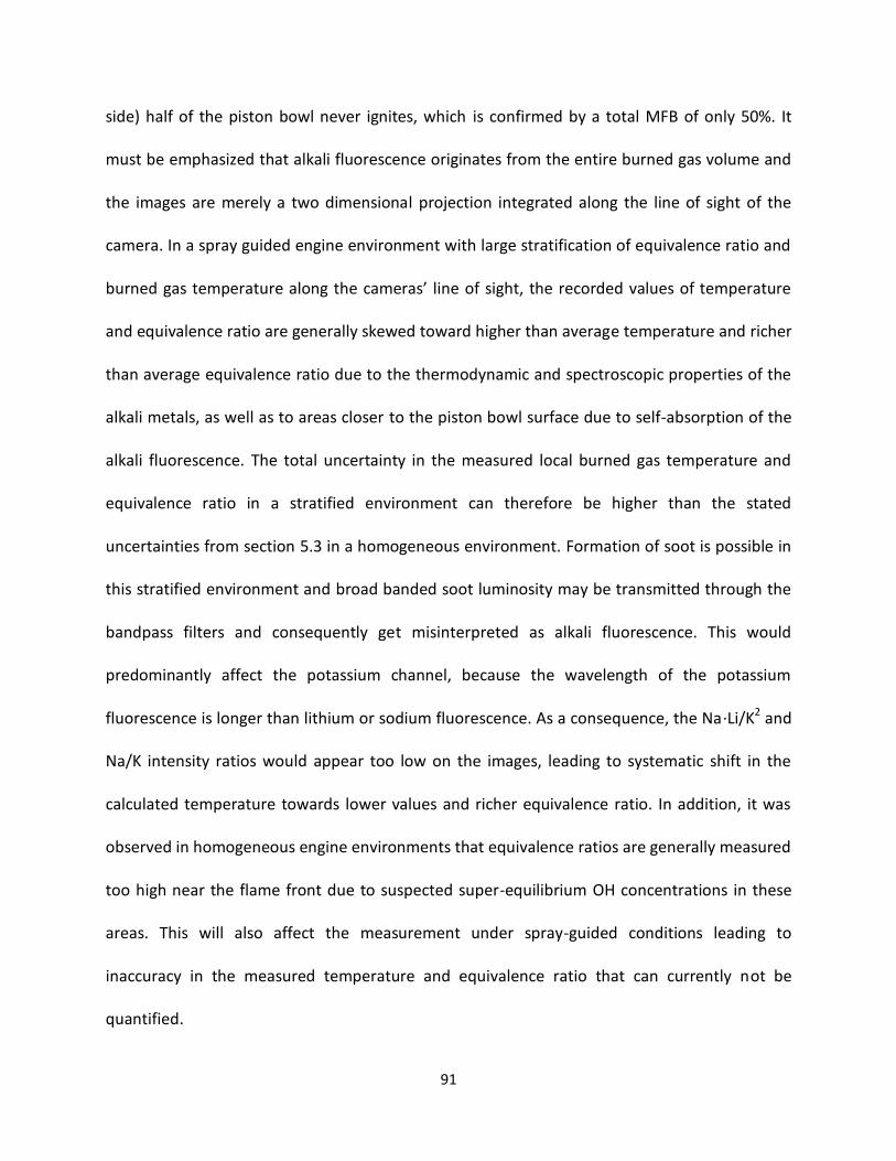
91

side) half of the piston bowl never ignites, which is confirmed by a total MFB of only 50%. It

must be emphasized that alkali fluorescence originates from the entire burned gas volume and

the images are merely a two dimensional projection integrated along the line of sight of the

camera. In a spray guided engine environment with large stratification of equivalence ratio and

burned gas temperature along the cameras’ line of sight, the recorded values of temperature

and equivalence ratio are generally skewed toward higher than average temperature and richer

than average equivalence ratio due to the thermodynamic and spectroscopic properties of the

alkali metals, as well as to areas closer to the piston bowl surface due to self-absorption of the

alkali fluorescence. The total uncertainty in the measured local burned gas temperature and

equivalence ratio in a stratified environment can therefore be higher than the stated

uncertainties from section 5.3 in a homogeneous environment. Formation of soot is possible in

this stratified environment and broad banded soot luminosity may be transmitted through the

bandpass filters and consequently get misinterpreted as alkali fluorescence. This would

predominantly affect the potassium channel, because the wavelength of the potassium

fluorescence is longer than lithium or sodium fluorescence. As a consequence, the Na·Li/K2 and

Na/K intensity ratios would appear too low on the images, leading to systematic shift in the

calculated temperature towards lower values and richer equivalence ratio. In addition, it was

observed in homogeneous engine environments that equivalence ratios are generally measured

too high near the flame front due to suspected super-equilibrium OH concentrations in these

areas. This will also affect the measurement under spray-guided conditions leading to

inaccuracy in the measured temperature and equivalence ratio that can currently not be

quantified.

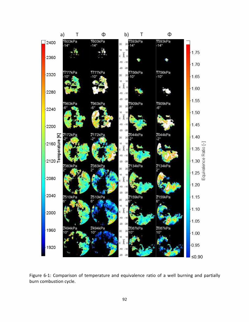
92

Figure 6-1: Comparison of temperature and equivalence ratio of a well burning and partially burn combustion cycle.

T TΦ Φ

≤0.90

a) b)

93

6.2 Improved experimental setup for spray-guided engine experiments

The three camera setup shown in Figure 5-1 was modified to improve the signal to noise ratio

of the lithium fluorescence in cold and lean burned gas zones and to better suppress soot

luminosity. Two Phantom V7.1 cameras recorded the sodium fluorescence at 589.0 and 589.6

nm and potassium fluorescence at 766.5 nm, respectively. A Vision Research Phantom V710

with a higher quantum efficiency of 35% near 671 nm was used to record both lithium

fluorescence lines.95 The lens mounted filters were replaced by customized narrow-banded

filters purchased from Omega Optical with center wavelengths at 589.0 nm (FWHM 2.0 nm,

50% peak transmission, 50 mm diameter), 670.8 nm (FWHM 1.0 nm, 30% peak transmission, 50

mm diameter) and 766.5 nm (FWHM 1.0 nm, 40% peak transmission, 50 mm diameter).

Experiments in stratified engine environments without alkali fuel additives showed a total

suppression of the soot luminosity even under high-sooting operating conditions. The

measured transmission spectra of the narrow banded bandpass filters are shown in Figure 6-2.

94

Figure 6-2: Measured transmission spectra of the lens mounted bandpass filters with FWHM of 1 nm and 2 nm, respectively, used during stratified engine operation to suppress soot luminosity.

6.3 Analysis of spray-guided, double-injected engine operation

A spray-guided engine operating condition with double injection was recorded and is displayed

in Figure 6-3. Engine speed was 800 rpm, the end of the first (EOI-1) and second injection (EOI-

2) were set to -21° and -12° aTDC, respectively, and the spark timing was set to -19° aTDC. The

total amount of fuel injected was 4.2 mg/cycle resulting in an IMEP of 112 kPa. The fuel

metering system was not instrumented to measure the amount of fuel injected individually for

the first and second injection. The images are ensemble averaged over 30 cycles and show the

0

5

10

15

20

25

30

35

667 669 671 673 675 677

Tra

nsm

issio

n [%

]

Wavelength [nm]

05

10152025303540455055

584 586 588 590 592 594 596

Tra

nsm

issio

n [%

]

Wavelength [nm]

0

5

10

15

20

25

30

35

40

45

763 764 765 766 767 768 769 770 771

Tra

nsm

issio

n [%

]

Wavelength [nm]

95

initial expansion of the burned gas cloud after the first injection and the leaning out of this zone

as more oxygen is entrained from the surrounding zones. As the second injection event takes

place at -12° aTDC, the local equivalence ratio in the center region becomes rich while the local

burned gas temperature cools off due to the evaporation of the liquid fuel. Further entrainment

of oxygen from unburned areas during the course of the combustion cycle leans out the burned

gas zone. Generally the equivalence ratio remains higher around the perimeter of the visible

cylinder bowl.

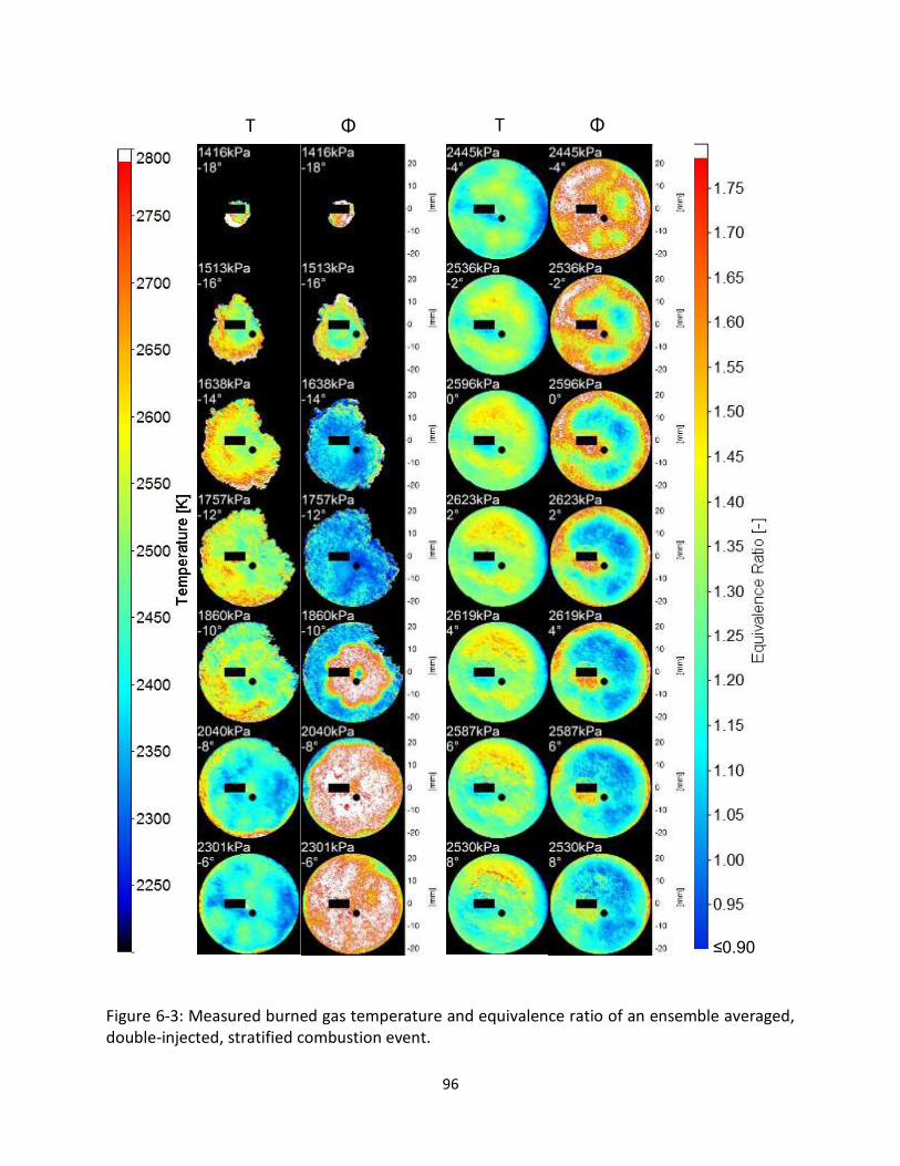
96

Figure 6-3: Measured burned gas temperature and equivalence ratio of an ensemble averaged, double-injected, stratified combustion event.

T TΦ Φ

≤0.90

97

6.4 Analysis of the effect of different injectors on engine combustion

Figure 6-4 shows a comparison of a 100-cycle ensemble average of identical engine operating

conditions with different injectors. The engine was run at 2000 rpm with 20% dilution of the

intake air with nitrogen. Both injection and ignition timing were set to -36° aTDC with 7.7 mg of

fuel injected per cycle. Both injectors are 8-hole injectors of the same manufacturer and model

generation with 60° spray angle. The length over diameter ratio of the injector holes used in

Figure 6-4a was L/D=2.4 and in Figure 6-4b L/D=2.0. This small parameter variation has a very

minor impact on engine performance with the average IMEP being 240 kPa for the L/D=2.4

injector and 235kPa for the L/D=2.0 injector. Previous studies have shown that a variation of

the L/D ratio can significantly influence the spray plume angle and change the spray and fuel-air

mixing characteristics. Larger L/D ratios generally produce a narrower cone angle with better

plume separation, while smaller L/D ratios produce wider cone angles that can lead to plume

interaction and the total collapse of the spray.96, 97 The burned gas temperature of the L/D=2.0

injector is approximately 200K lower than for the L/D=2.4 injector, which could be due to the

delayed evaporation of the fuel drawing heat from the burned gas zone. The equivalence ratio

is initially measured richer for the L/D=2.0 injector in the observed piston bowl area. Toward

the end of combustion the area near the perimeter of the piston bowl is significantly richer

than the center region. This is in good agreement with the assumption that the spray of the

L/D=2.0 injector might have collapsed hitting the piston and the possibility of liquid fuel

accumulating in the corner of the piston bowl, where it might not sufficiently mix with air and

consequently burn at very rich equivalence ratio. Simultaneous imaging of the injector spray

98

can provide additional insight and help develop a better understanding of the relation of

injector spray characteristics to combustion characteristics.

Figure 6-4: Comparison of measured burned gas temperature and equivalence ratio of ensemble averaged, single injected, stratified engine combustion cycles using two different injectors.

T TΦ Φa) b)

≤0.90

99

CHAPTER 7. Conclusion and future potential of this technique for three dimensional

measurements and endoscope imaging in all-metal engines

A spectroscopic combustion diagnostic tool was developed for the use on internal combustion

engines. The technique is based on the high-speed imaging of the natural fluorescence of alkali

metals in flames. The dominant chemical and physical processes that determine the

fluorescence intensity of lithium, sodium and potassium metals in the burned gas region of an

internal combustion engine are understood quantitatively within the uncertainty of various

measured and calculated quantities such as equivalence ratio and burned gas temperature.

Both Na/K and Na·Li/K2 fluorescence intensity ratios depend on burned gas temperature, but

the Na/K fluorescence ratio also depends on equivalence ratio and pressure. Using both

fluorescence ratios simultaneously makes this a particularly useful tool for the simultaneous

high-speed measurement of burned gas temperature and equivalence ratio under

homogeneous and stratified engine operation. The fact that no laser or image intensifier is

needed is a significant advantage over many other optical combustion diagnostic tools making

it highly applicable for engine combustion research. The dominant source of uncertainty in this

study was the calculation of burned gas temperature using a zero dimensional GT-Power engine

combustion model. The accuracy of this calculation is lowest for early flame kernels, where a

small error in the convective heat transfer calculation results in large discrepancies of the

calculated burned gas temperature.

100

Additional accuracy limitation for stratified engine operation stems from the fact that each

camera only sees a 2D projection of the 3D burned gas zone and the measured temperatures

and equivalence ratios are therefore merely weighted averages along the cameras’ line of sight.

Unknown depth and stratification of the burned gas cloud therefore limit the quantitative

applicability of this measurement technique in stratified combustion environments. This could

be improved by imaging from multiple views to allow for valid approximations of the

stratification of these two quantities. Useful applications of this tool are the investigation of

partial burns and cyclic variability under stratified engine operation as well as comparing the

effects of engine hardware or design changes on the combustion process. In combination with

spray and soot imaging, this tool can be used for injector and combustion chamber geometry

optimization.

The quantitative examination of small flame kernels is limited by the unknown absorption

length. Imaging from multiple views could in part lift this limitation. It is possible to fully avoid

self-absorption of the alkali fluorescence by reducing the alkali fuel concentration by a factor of

approximately 500. In this case less than 2% of the emitted fluorescence would get reabsorbed.

Overall, this would result in measured fluorescence intensities being lower by a factor of 100,

which is too weak to record the fluorescence with the existing imaging setup. The use of high

speed image intensifiers would be required to amplify the light sufficiently. While the use of

image intensifiers introduces additional shot noise to the images, the overall accuracy of the

equivalence ratio and temperature measurement of small flame kernels might still be improved

substantially by avoiding self-absorption.

101

In addition, the mismatch of recorded burned gas temperature and equivalence ratio in the

early flame kernel and near the perimeter of the burned gas zone indicate that the assumption

of perfect chemical equilibrium in the burned gas zone is not valid near the flame front.

Previous studies have shown super-equilibrium concentrations of hydroxyl and hydrogen

radicals in these areas, which would affect the equilibration of alkali atom concentration and

consequently result in inaccuracies in the obtained temperature and equivalence ratio. A

quantitative investigation of the reaction kinetics would be required to improve accuracy of this

tool near the flame front region. Unfortunately, not enough literature data is currently available

to attempt the inclusion of reaction kinetics for alkali containing iso-octane fuel in engine

combustion.

The experimental approach of this technique could be simplified further by replacing the three

high-speed cameras that were used in this study by relatively inexpensive photo-multipliers.

This would remove the capability of two dimensional spatial resolution of burned gas

temperature and equivalence ratio that was demonstrated in this study. However, in cases

where spatial resolution is not required, this approach would significantly reduce experimental

complexity and cost. Appendix D shows how the spatially averaged fluorescence recorded by

photo-multipliers can be used to obtain values for global burned gas temperature and

equivalence ratio with small deviation from the spatially resolved fluorescence imaging using

high-speed cameras. The model that was developed in this study to quantify the temperature,

pressure and equivalence ratio dependence of the alkali fluorescence intensity could be

integrated in a simple machine that acquires the fluorescence intensity using photo-multipliers

and automates the conversion of recorded fluorescence intensities into burned gas

102

temperature and equivalence ratio with little requirement for user input. Such a device could

be of high interest for the use in industrial engine development environments, where fast and

reliable results and hence reduction of experimental complexity are of high importance.

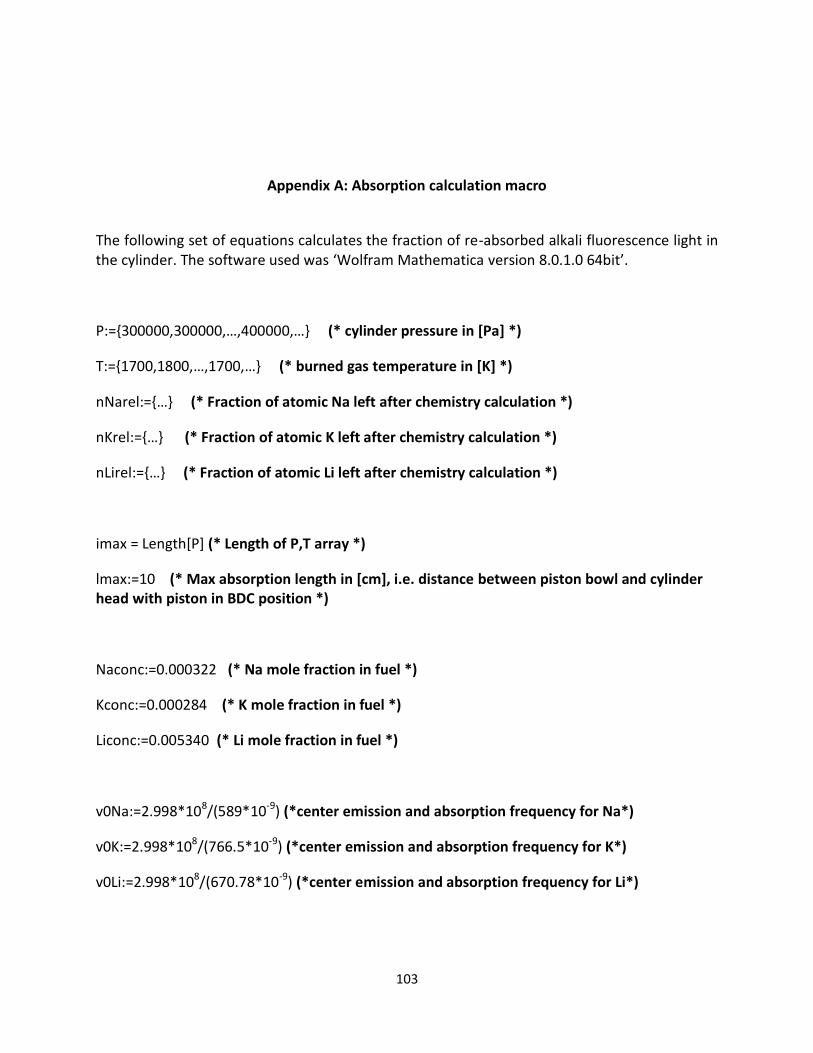
103

Appendix A: Absorption calculation macro

The following set of equations calculates the fraction of re-absorbed alkali fluorescence light in the cylinder. The software used was ‘Wolfram Mathematica version 8.0.1.0 64bit’.

P:={300000,300000,…,400000,…} (* cylinder pressure in [Pa] *)

T:={1700,1800,…,1700,…} (* burned gas temperature in [K] *)

nNarel:={…} (* Fraction of atomic Na left after chemistry calculation *)

nKrel:={…} (* Fraction of atomic K left after chemistry calculation *)

nLirel:={…} (* Fraction of atomic Li left after chemistry calculation *)

imax = Length[P] (* Length of P,T array *)

lmax:=10 (* Max absorption length in [cm], i.e. distance between piston bowl and cylinder head with piston in BDC position *)

Naconc:=0.000322 (* Na mole fraction in fuel *)

Kconc:=0.000284 (* K mole fraction in fuel *)

Liconc:=0.005340 (* Li mole fraction in fuel *)

v0Na:=2.998*108/(589*10-9) (*center emission and absorption frequency for Na*)

v0K:=2.998*108/(766.5*10-9) (*center emission and absorption frequency for K*)

v0Li:=2.998*108/(670.78*10-9) (*center emission and absorption frequency for Li*)

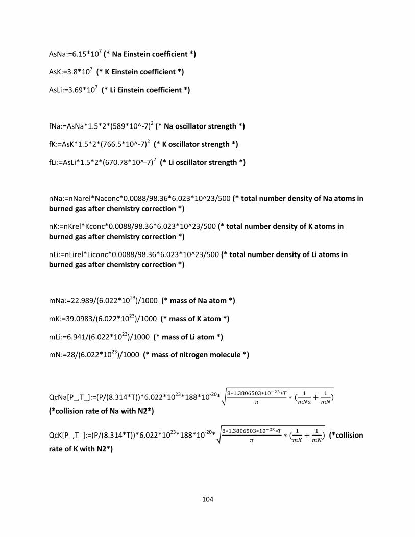
104

AsNa:=6.15*107 (* Na Einstein coefficient *)

AsK:=3.8*107 (* K Einstein coefficient *)

AsLi:=3.69*107 (* Li Einstein coefficient *)

fNa:=AsNa*1.5*2*(589*10^-7)2 (* Na oscillator strength *)

fK:=AsK*1.5*2*(766.5*10^-7)2 (* K oscillator strength *)

fLi:=AsLi*1.5*2*(670.78*10^-7)2 (* Li oscillator strength *)

nNa:=nNarel*Naconc*0.0088/98.36*6.023*10^23/500 (* total number density of Na atoms in burned gas after chemistry correction *)

nK:=nKrel*Kconc*0.0088/98.36*6.023*10^23/500 (* total number density of K atoms in burned gas after chemistry correction *)

nLi:=nLirel*Liconc*0.0088/98.36*6.023*10^23/500 (* total number density of Li atoms in burned gas after chemistry correction *)

mNa:=22.989/(6.022*1023)/1000 (* mass of Na atom *)

mK:=39.0983/(6.022*1023)/1000 (* mass of K atom *)

mLi:=6.941/(6.022*1023)/1000 (* mass of Li atom *)

mN:=28/(6.022*1023)/1000 (* mass of nitrogen molecule *)

QcNa[P_,T_]:=(P/(8.314*T))*6.022*1023*188*10-20*√

(

)

(*collision rate of Na with N2*)

QcK[P_,T_]:=(P/(8.314*T))*6.022*1023*188*10-20*√

(

) (*collision

rate of K with N2*)

105

QcLi[P_,T_]:=(P/(8.314*T))*6.022*1023*146*10-20*√

(

)

(*collision rate of Li with N2*)

vDNa[T_,mNa_,v0Na_]:=2*√ [ ] *v0Na/(2.998*108) (* Doppler broadened line width of Na *)

vDK[T_,mK_,v0K_]:=2*√ [ ] *v0K/(2.998*108) (* Doppler

broadened line width of K *)

vDLi[T_,mLi_,v0Li_]:=2*√ [ ] *v0Li/(2.998*108) (*

Doppler broadened line width of Li *)

vLNa[AsNa_,QcNa_]:=(AsNa/(2*))+(QcNa/(2*)) (* Lorentz (i.e. natural + collision) broadened line width of Na *)

vLK[AsK_,QcK_]:=(AsK/(2*))+(QcK/(2*)) (* Lorentz (i.e. natural + collision) broadened line width of K *)

vLLi[AsLi_,QcLi_]:=(AsLi/(2*))+(QcLi/(2*)) (* Lorentz (i.e. natural + collision) broadened line width of Li *)

vVNa[vDNa_,vLNa_]:=1/2*vLNa+√

(* Voigt (i.e. Lorentz + Doppler)

broadened line width of Na *)

vVK[vDK_,vLK_]:=1/2*vLK+√

(* Voigt (i.e. Lorentz + Doppler) broadened line

width of K *)

vVLi[vDLi_,vLLi_]:=1/2*vLLi+√

(* Voigt (i.e. Lorentz + Doppler) broadened

line width of Li *)

SVNa[vDNa_,vLNa_,v0Na_,vNa_,y_]:=((2*√ [ ])/(*√ ))*0.84*(vLNa/vDNa2)*( /((0.84*

vLNa/vDNa)2+(((vNa-v0Na)*2*√ [ ])/vDNa-y)2)) (*Voigt (i.e. Doppler + Lorentz) broadened

line profile of Na*)

106

SVNaint[vDNa_,vLNa_,v0Na_]:=NIntegrate[(2*√ [ ]))/(* √ )*0.84*vLNa/vDNa2* /((0.

84*vLNa/vDNa)2+(((vNa-v0Na)*2*√ [ ]))/vDNa-y)2),{vNa,v0Na-

(1/1000*v0Na),v0Na+(1/1000*v0Na)},{y,-Infinity,Infinity}] (*check if it integrates to 1*)

SVNaint[vDNa[T[[1]],mNa,v0Na],vLNa[AsNa,QcNa[P[[1]],T[[1]]]],v0Na]

SVK[vDK_,vLK_,v0K_,vK_,y_]:=((2*√ [ ])/(* √ ))*0.84*(vLK/vDK2)*( /((0.84*vLK/vDK)

2+(((vK-v0K)*2*√ [ ])/vDK-y)2)) (*Voigt (i.e. Doppler + Lorentz) broadened line profile of

K*)

SVKint[vDK_,vLK_,v0K_]:=NIntegrate[(2*√ [ ])/(* √ )*0.84*vLK/vDK2* /((0.84*vLK/v

DK)2+(((vK-v0K)*2*√ [ ])/vDK-y)2),{vK,v0K-(1/1000*v0K),v0K+(1/1000*v0K)},{y,-

Infinity,Infinity}] (*check if it integrates to 1*)

SVKint[vDK[T[[1]],mK,v0K],vLK[AsK,QcK[P[[1]],T[[1]]]],v0K]

SVLi[vDLi_,vLLi_,v0Li_,vLi_,y_]:=((2*√ [ ])/(* √ ))*0.84*(vLLi/vDLi2)*( /((0.84*vLLi/vD

Li)2+(((vLi-v0Li)*2*√ [ ])/vDLi-y)2)) (*Voigt (i.e. Doppler + Lorentz) broadened line profile

of K*)

SVLiint[vDLi_,vLLi_,v0Li_]:=NIntegrate[(2*√ [ ])/(* √ )*0.84*vLLi/vDLi2* /((0.84*vLLi/

vDLi)2+(((vLi-v0Li)*2*√ [ ])/vDLi-y)2),{vLi,v0Li-(1/1000*v0Li),v0Li+(1/1000*v0Li)},{y,-

Infinity,Infinity}] (*check if it integrates to 1*)

SVLiint[vDLi[T[[1]],mLi,v0Li],vLLi[AsLi,QcLi[P[[1]],T[[1]]]],v0Li]

kNa[SNa_,fNa]:=2.65*10-2*SNa*fNa (* spectral absorbtivity of Na *)

kK[SK_,fK]:=2.65*10-2*SK*fK (* spectral absorbtivity of K *)

kLi[SLi_,fLi]:=2.65*10-2*SLi*fLi (* spectral absorbtivity of Li *)

AVNa[SVNa_,kNa_,nNa_,vVNa_,lmax_]:=NIntegrate[SVNa/lmax*(1- ),{vNa,v0Na-10*vVNa,v0Na+10*vVNa},{l,0,lmax},{y,-Infinity,Infinity}] (* fraction of reabsorbed Na fluorescence *)

107

AVK[SVK_,kK_,nK_,vVK_,lmax_]:=NIntegrate[SVK/lmax*(1- ),{vK,v0K-10*vVK,v0K+10*vVK},{l,0,lmax},{y,-Infinity,Infinity}] (* fraction of reabsorbed K fluorescence *)

AVLi[SVLi_,kLi_,nLi_,vVLi_,lmax_]:=NIntegrate[SVLi/lmax*(1- ),{vLi,v0Li-10*vVLi,v0Li+10*vVLi},{l,0,lmax},{y,-Infinity,Infinity}] (* fraction of reabsorbed Li fluorescence *)

For[i=1,i<imax+1,i++,Print[AVNa[SVNa[vDNa[T[[i]],mNa,v0Na],vLNa[AsNa,QcNa[P[[i]],T[[i]]]],v0Na,vNa,y],kNa[SVNa[vDNa[T[[i]],mNa,v0Na],vLNa[AsNa,QcNa[P[[i]],T[[i]]]],v0Na,vNa,y],fNa],nNa[[i]],vVNa[vDNa[T[[i]],mNa,v0Na],vLNa[AsNa,QcNa[P[[i]],T[[i]]]]],lmax]]] (* Calculate for all P, T, n in array *)

For[i=1,i<imax+1,i++,Print[AVK[SVK[vDK[T[[i]],mK,v0K],vLK[AsK,QcK[P[[i]],T[[i]]]],v0K,vK,y],kK[SVK[vDK[T[[i]],mK,v0K],vLK[AsK,QcK[P[[i]],T[[i]]]],v0K,vK,y],fK],nK[[i]],vVK[vDK[T[[i]],mK,v0K],vLK[AsK,QcK[P[[i]],T[[i]]]]],lmax]]] (* Calculate for all P, T, n in array *)

For[i=1,i<imax+1,i++,Print[AVLi[SVLi[vDLi[T[[i]],mLi,v0Li],vLLi[AsLi,QcLi[P[[i]],T[[i]]]],v0Li,vLi,y],kLi[SVLi[vDLi[T[[i]],mLi,v0Li],vLLi[AsLi,QcLi[P[[i]],T[[i]]]],v0Li,vLi,y],fLi],nLi[[i]],vVLi[vDLi[T[[i]],mLi,v0Li],vLLi[AsLi,QcLi[P[[i]],T[[i]]]]],lmax]]] (* Calculate for all P, T, n in array *)

108

Appendix B: Flow chart for building fluorescence intensity database

Chem

ical E

quilib

rium

Calc

ula

tion

T, P

, Ф

Excite

d S

tate

Po

pu

latio

n

Bo

ltzm

an

n d

istrib

utio

n

T

Absorp

tion C

alc

ula

tion

xi

T, P

Data

base

for T

, P, Ф

de

pe

nd

en

ce

of N

a/K

fluore

scence in

tensity

ratio

Da

tab

ase

for T

, P, Ф

dependence o

f Na

·Li/K

2

fluore

scence in

tensity

ratio

xi

Tri

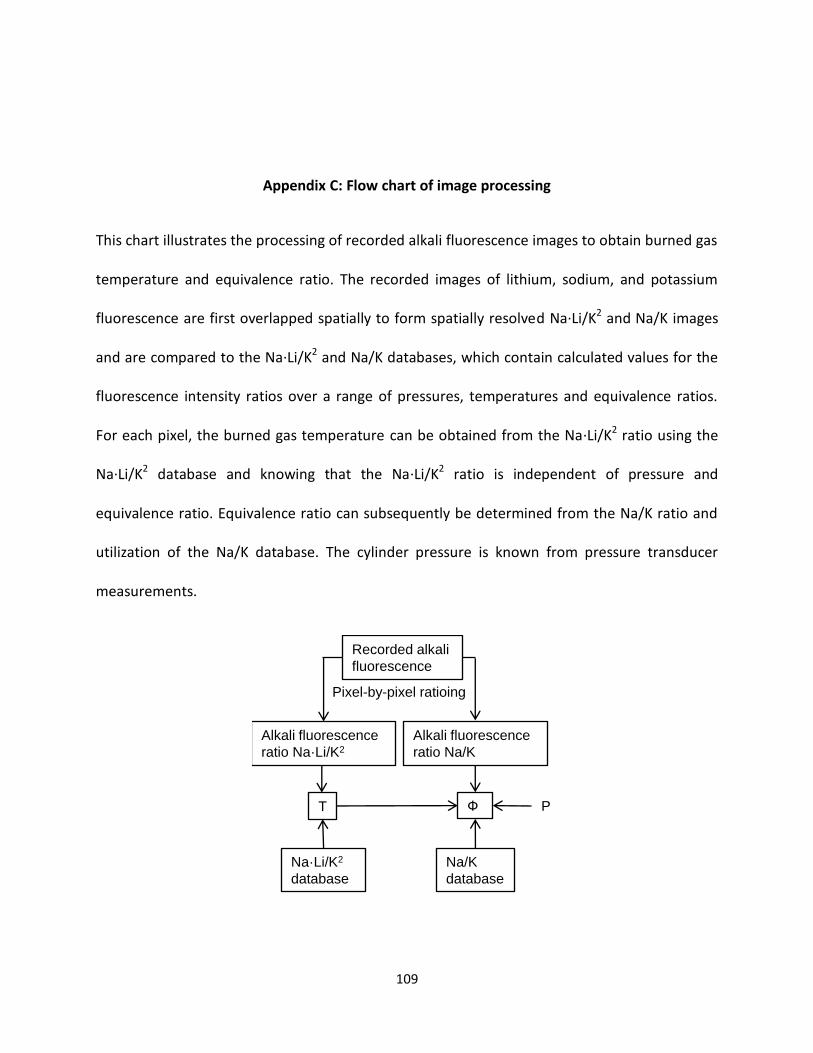
109

Appendix C: Flow chart of image processing

This chart illustrates the processing of recorded alkali fluorescence images to obtain burned gas

temperature and equivalence ratio. The recorded images of lithium, sodium, and potassium

fluorescence are first overlapped spatially to form spatially resolved Na·Li/K2 and Na/K images

and are compared to the Na·Li/K2 and Na/K databases, which contain calculated values for the

fluorescence intensity ratios over a range of pressures, temperatures and equivalence ratios.

For each pixel, the burned gas temperature can be obtained from the Na·Li/K2 ratio using the

Na·Li/K2 database and knowing that the Na·Li/K2 ratio is independent of pressure and

equivalence ratio. Equivalence ratio can subsequently be determined from the Na/K ratio and

utilization of the Na/K database. The cylinder pressure is known from pressure transducer

measurements.

Na·Li/K2

database

Recorded alkali

fluorescence

Alkali fluorescence

ratio Na·Li/K2

T P

Pixel-by-pixel ratioing

Alkali fluorescence

ratio Na/K

Ф

Na/K

database

110

Appendix D: T and Ф measurements using photo-multipliers

The following flow chart compares the calculation of spatially resolved burned gas temperature

and equivalence ratio from alkali fluorescence imaging on a camera (left path) versus the

calculation of burned gas temperature and equivalence ratio from spatially averaged alkali

fluorescence recordings on photo-multipliers (right path). If alkali fluorescence is recorded with

spatial resolution on cameras, burned gas temperature and equivalence ratio can be calculated

for each pixel separately following the left pathway in the flow chart. Photo-multipliers,

however, would record only the spatial average of the alkali fluorescence and a pixel-by-pixel

calculation of burned gas temperature and equivalence ratio is therefore not possible. Instead,

the spatially averaged lithium, sodium and potassium fluorescence must be used to compute a

global burned gas temperature and equivalence ratio following the right pathway in the flow

chart. Due to the non-linear relationship of alkali fluorescence intensity to burned gas

temperature and equivalence ratio, it is not expected that the burned gas temperature and

equivalence ratio calculated from photo-multiplier recordings equal the average of the spatially

resolved burned gas temperature and equivalence ratio imaging. In this example of nearly

homogeneous engine operation, the error in computed burned gas temperature and

equivalence ratio from photo-multiplier measurements is 4K and 0.01, respectively. This error is

small compared to the overall accuracy uncertainty of T ±100K and Ф ±0.03 and justifies the use

of photo-multipliers instead of high-speed cameras to reduce cost and complexity of the

measurement apparatus in cases where spatial resolution is not needed.

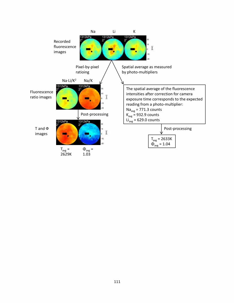
111

Na Li K

Na·Li/K2 Na/K

Tavg = 2629K

Φavg = 1.03

Pixel-by-pixel ratioing

Post-processing

The spatial average of the fluorescence intensities after correction for camera exposure time corresponds to the expected reading from a photo-multiplier:Naavg = 771.3 countsKavg = 932.9 countsLiavg = 629.0 counts

Tavg = 2633KΦavg = 1.04

Post-processing

Spatial average as measured by photo-multipliers

Recorded fluorescence images

Fluorescence ratio images

T and Фimages

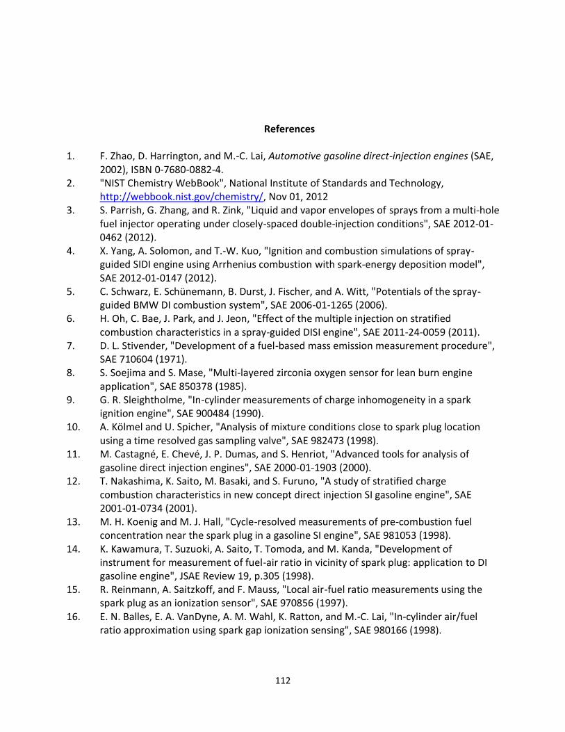
112

References

1. F. Zhao, D. Harrington, and M.-C. Lai, Automotive gasoline direct-injection engines (SAE, 2002), ISBN 0-7680-0882-4.

2. "NIST Chemistry WebBook", National Institute of Standards and Technology, http://webbook.nist.gov/chemistry/, Nov 01, 2012

3. S. Parrish, G. Zhang, and R. Zink, "Liquid and vapor envelopes of sprays from a multi-hole fuel injector operating under closely-spaced double-injection conditions", SAE 2012-01-0462 (2012).

4. X. Yang, A. Solomon, and T.-W. Kuo, "Ignition and combustion simulations of spray-guided SIDI engine using Arrhenius combustion with spark-energy deposition model", SAE 2012-01-0147 (2012).

5. C. Schwarz, E. Schünemann, B. Durst, J. Fischer, and A. Witt, "Potentials of the spray-guided BMW DI combustion system", SAE 2006-01-1265 (2006).

6. H. Oh, C. Bae, J. Park, and J. Jeon, "Effect of the multiple injection on stratified combustion characteristics in a spray-guided DISI engine", SAE 2011-24-0059 (2011).

7. D. L. Stivender, "Development of a fuel-based mass emission measurement procedure", SAE 710604 (1971).

8. S. Soejima and S. Mase, "Multi-layered zirconia oxygen sensor for lean burn engine application", SAE 850378 (1985).

9. G. R. Sleightholme, "In-cylinder measurements of charge inhomogeneity in a spark ignition engine", SAE 900484 (1990).

10. A. Kölmel and U. Spicher, "Analysis of mixture conditions close to spark plug location using a time resolved gas sampling valve", SAE 982473 (1998).

11. M. Castagné, E. Chevé, J. P. Dumas, and S. Henriot, "Advanced tools for analysis of gasoline direct injection engines", SAE 2000-01-1903 (2000).

12. T. Nakashima, K. Saito, M. Basaki, and S. Furuno, "A study of stratified charge combustion characteristics in new concept direct injection SI gasoline engine", SAE 2001-01-0734 (2001).

13. M. H. Koenig and M. J. Hall, "Cycle-resolved measurements of pre-combustion fuel concentration near the spark plug in a gasoline SI engine", SAE 981053 (1998).

14. K. Kawamura, T. Suzuoki, A. Saito, T. Tomoda, and M. Kanda, "Development of instrument for measurement of fuel-air ratio in vicinity of spark plug: application to DI gasoline engine", JSAE Review 19, p.305 (1998).

15. R. Reinmann, A. Saitzkoff, and F. Mauss, "Local air-fuel ratio measurements using the spark plug as an ionization sensor", SAE 970856 (1997).

16. E. N. Balles, E. A. VanDyne, A. M. Wahl, K. Ratton, and M.-C. Lai, "In-cylinder air/fuel ratio approximation using spark gap ionization sensing", SAE 980166 (1998).

http://webbook.nist.gov/chemistry/

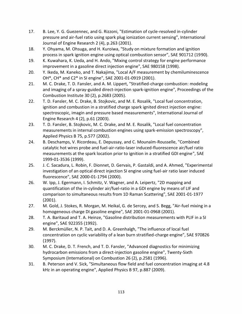
113

17. B. Lee, Y. G. Guezennec, and G. Rizzoni, "Estimation of cycle-resolved in-cylinder pressure and air-fuel ratio using spark plug ionization current sensing", International Journal of Engine Research 2 (4), p.263 (2001).

18. Y. Ohyama, M. Ohsuga, and H. Kuroiwa, "Study on mixture formation and ignition process in spark ignition engine using optical combustion sensor", SAE 901712 (1990).

19. K. Kuwahara, K. Ueda, and H. Ando, "Mixing control strategy for engine performance improvement in a gasoline direct injection engine", SAE 980158 (1998).

20. Y. Ikeda, M. Kaneko, and T. Nakajima, "Local A/F measurement by chemiluminescence OH*, CH* and C2* in SI engine", SAE 2001-01-0919 (2001).

21. M. C. Drake, T. D. Fansler, and A. M. Lippert, "Stratified-charge combustion: modeling and imaging of a spray-guided direct-injection spark-ignition engine", Proceedings of the Combustion Institute 30 (2), p.2683 (2005).

22. T. D. Fansler, M. C. Drake, B. Stojkovic, and M. E. Rosalik, "Local fuel concentration, ignition and combustion in a stratified charge spark ignited direct injection engine: spectroscopic, imagin and pressure based measurements", International Journal of Engine Research 4 (2), p.61 (2003).

23. T. D. Fansler, B. Stojkovic, M. C. Drake, and M. E. Rosalik, "Local fuel concentration measurements in internal combustion engines using spark-emission spectroscopy", Applied Physics B 75, p.577 (2002).

24. B. Deschamps, V. Ricordeau, E. Depussay, and C. Mounaïm-Rousselle, "Combined catalytic hot wires probe and fuel-air-ratio-laser induced-fluorescence air/fuel ratio measurements at the spark location prior to ignition in a stratified GDI engine", SAE 1999-01-3536 (1999).

25. J. C. Sacadura, L. Robin, F. Dionnet, D. Gervais, P. Gastaldi, and A. Ahmed, "Experimental investigation of an optical direct injection SI engine using fuel-air ratio laser induced fluorescence", SAE 2000-01-1794 (2000).

26. W. Ipp, J. Egermann, I. Schmitz, V. Wagner, and A. Leipertz, "2D mapping and quantification of the in-cylinder air/fuel-ratio in a GDI engine by means of LIF and comparison to simultaneous results from 1D Raman Scattering", SAE 2001-01-1977 (2001).

27. M. Gold, J. Stokes, R. Morgan, M. Heikal, G. de Sercey, and S. Begg, "Air-fuel mixing in a homogeneous charge DI gasoline engine", SAE 2001-01-0968 (2001).

28. T. A. Baritaud and T. A. Heinze, "Gasoline distribution measurements with PLIF in a SI engine", SAE 922355 (1992).

29. M. Berckmüller, N. P. Tait, and D. A. Greenhalgh, "The influence of local fuel concentration on cyclic variability of a lean burn stratified-charge engine", SAE 970826 (1997).

30. M. C. Drake, D. T. French, and T. D. Fansler, "Advanced diagnostics for minimizing hydrocarbon emissions from a direct-injection gasoline engine", Twenty-Sixth Symposium (International) on Combustion 26 (2), p.2581 (1996).

31. B. Peterson and V. Sick, "Simultaneous flow field and fuel concentration imaging at 4.8 kHz in an operating engine", Applied Physics B 97, p.887 (2009).

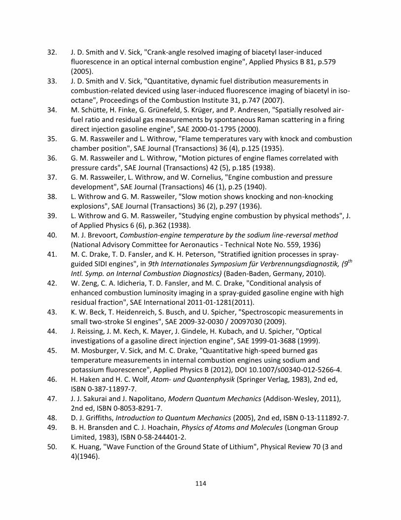
114

32. J. D. Smith and V. Sick, "Crank-angle resolved imaging of biacetyl laser-induced fluorescence in an optical internal combustion engine", Applied Physics B 81, p.579 (2005).

33. J. D. Smith and V. Sick, "Quantitative, dynamic fuel distribution measurements in combustion-related deviced using laser-induced fluorescence imaging of biacetyl in iso-octane", Proceedings of the Combustion Institute 31, p.747 (2007).

34. M. Schütte, H. Finke, G. Grünefeld, S. Krüger, and P. Andresen, "Spatially resolved air-fuel ratio and residual gas measurements by spontaneous Raman scattering in a firing direct injection gasoline engine", SAE 2000-01-1795 (2000).

35. G. M. Rassweiler and L. Withrow, "Flame temperatures vary with knock and combustion chamber position", SAE Journal (Transactions) 36 (4), p.125 (1935).

36. G. M. Rassweiler and L. Withrow, "Motion pictures of engine flames correlated with pressure cards", SAE Journal (Transactions) 42 (5), p.185 (1938).

37. G. M. Rassweiler, L. Withrow, and W. Cornelius, "Engine combustion and pressure development", SAE Journal (Transactions) 46 (1), p.25 (1940).

38. L. Withrow and G. M. Rassweiler, "Slow motion shows knocking and non-knocking explosions", SAE Journal (Transactions) 36 (2), p.297 (1936).

39. L. Withrow and G. M. Rassweiler, "Studying engine combustion by physical methods", J. of Applied Physics 6 (6), p.362 (1938).

40. M. J. Brevoort, Combustion-engine temperature by the sodium line-reversal method (National Advisory Committee for Aeronautics - Technical Note No. 559, 1936)

41. M. C. Drake, T. D. Fansler, and K. H. Peterson, "Stratified ignition processes in spray-guided SIDI engines", in 9th Internationales Symposium für Verbrennungsdiagnostik, (9th Intl. Symp. on Internal Combustion Diagnostics) (Baden-Baden, Germany, 2010).

42. W. Zeng, C. A. Idicheria, T. D. Fansler, and M. C. Drake, "Conditional analysis of enhanced combustion luminosity imaging in a spray-guided gasoline engine with high residual fraction", SAE International 2011-01-1281(2011).

43. K. W. Beck, T. Heidenreich, S. Busch, and U. Spicher, "Spectroscopic measurements in small two-stroke SI engines", SAE 2009-32-0030 / 20097030 (2009).

44. J. Reissing, J. M. Kech, K. Mayer, J. Gindele, H. Kubach, and U. Spicher, "Optical investigations of a gasoline direct injection engine", SAE 1999-01-3688 (1999).

45. M. Mosburger, V. Sick, and M. C. Drake, "Quantitative high-speed burned gas temperature measurements in internal combustion engines using sodium and potassium fluorescence", Applied Physics B (2012), DOI 10.1007/s00340-012-5266-4.

46. H. Haken and H. C. Wolf, Atom- und Quantenphysik (Springer Verlag, 1983), 2nd ed, ISBN 0-387-11897-7.

47. J. J. Sakurai and J. Napolitano, Modern Quantum Mechanics (Addison-Wesley, 2011), 2nd ed, ISBN 0-8053-8291-7.

48. D. J. Griffiths, Introduction to Quantum Mechanics (2005), 2nd ed, ISBN 0-13-111892-7. 49. B. H. Bransden and C. J. Hoachain, Physics of Atoms and Molecules (Longman Group

Limited, 1983), ISBN 0-58-244401-2. 50. K. Huang, "Wave Function of the Ground State of Lithium", Physical Review 70 (3 and

4)(1946).

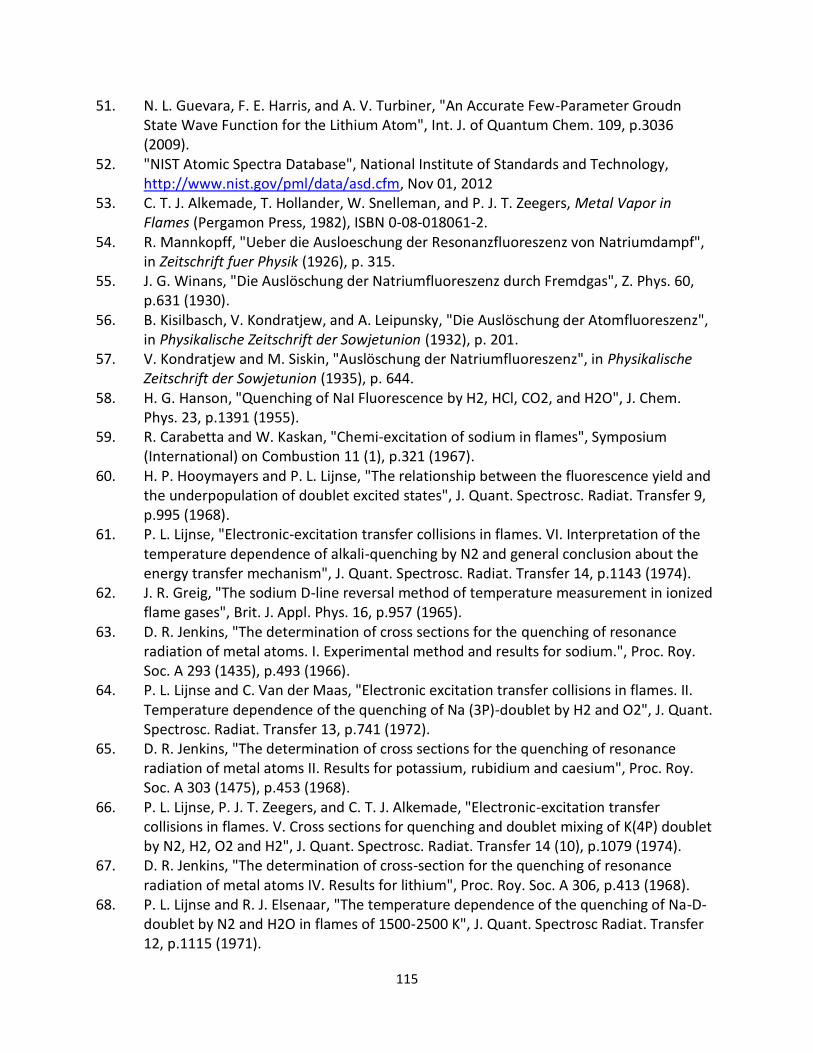
115

51. N. L. Guevara, F. E. Harris, and A. V. Turbiner, "An Accurate Few-Parameter Groudn State Wave Function for the Lithium Atom", Int. J. of Quantum Chem. 109, p.3036 (2009).

52. "NIST Atomic Spectra Database", National Institute of Standards and Technology, http://www.nist.gov/pml/data/asd.cfm, Nov 01, 2012

53. C. T. J. Alkemade, T. Hollander, W. Snelleman, and P. J. T. Zeegers, Metal Vapor in Flames (Pergamon Press, 1982), ISBN 0-08-018061-2.

54. R. Mannkopff, "Ueber die Ausloeschung der Resonanzfluoreszenz von Natriumdampf", in Zeitschrift fuer Physik (1926), p. 315.

55. J. G. Winans, "Die Auslöschung der Natriumfluoreszenz durch Fremdgas", Z. Phys. 60, p.631 (1930).

56. B. Kisilbasch, V. Kondratjew, and A. Leipunsky, "Die Auslöschung der Atomfluoreszenz", in Physikalische Zeitschrift der Sowjetunion (1932), p. 201.

57. V. Kondratjew and M. Siskin, "Auslöschung der Natriumfluoreszenz", in Physikalische Zeitschrift der Sowjetunion (1935), p. 644.

58. H. G. Hanson, "Quenching of NaI Fluorescence by H2, HCl, CO2, and H2O", J. Chem. Phys. 23, p.1391 (1955).

59. R. Carabetta and W. Kaskan, "Chemi-excitation of sodium in flames", Symposium (International) on Combustion 11 (1), p.321 (1967).

60. H. P. Hooymayers and P. L. Lijnse, "The relationship between the fluorescence yield and the underpopulation of doublet excited states", J. Quant. Spectrosc. Radiat. Transfer 9, p.995 (1968).

61. P. L. Lijnse, "Electronic-excitation transfer collisions in flames. VI. Interpretation of the temperature dependence of alkali-quenching by N2 and general conclusion about the energy transfer mechanism", J. Quant. Spectrosc. Radiat. Transfer 14, p.1143 (1974).

62. J. R. Greig, "The sodium D-line reversal method of temperature measurement in ionized flame gases", Brit. J. Appl. Phys. 16, p.957 (1965).

63. D. R. Jenkins, "The determination of cross sections for the quenching of resonance radiation of metal atoms. I. Experimental method and results for sodium.", Proc. Roy. Soc. A 293 (1435), p.493 (1966).

64. P. L. Lijnse and C. Van der Maas, "Electronic excitation transfer collisions in flames. II. Temperature dependence of the quenching of Na (3P)-doublet by H2 and O2", J. Quant. Spectrosc. Radiat. Transfer 13, p.741 (1972).

65. D. R. Jenkins, "The determination of cross sections for the quenching of resonance radiation of metal atoms II. Results for potassium, rubidium and caesium", Proc. Roy. Soc. A 303 (1475), p.453 (1968).

66. P. L. Lijnse, P. J. T. Zeegers, and C. T. J. Alkemade, "Electronic-excitation transfer collisions in flames. V. Cross sections for quenching and doublet mixing of K(4P) doublet by N2, H2, O2 and H2", J. Quant. Spectrosc. Radiat. Transfer 14 (10), p.1079 (1974).

67. D. R. Jenkins, "The determination of cross-section for the quenching of resonance radiation of metal atoms IV. Results for lithium", Proc. Roy. Soc. A 306, p.413 (1968).

68. P. L. Lijnse and R. J. Elsenaar, "The temperature dependence of the quenching of Na-D-doublet by N2 and H2O in flames of 1500-2500 K", J. Quant. Spectrosc Radiat. Transfer 12, p.1115 (1971).

http://www.nist.gov/pml/data/asd.cfm

116

69. P. L. Lijnse, P. J. T. Zeegers, and C. T. J. Alkemade, "Electronic-excitation transfer collisions in flames. III. Cross sections for quenching and doublet mixing of Rb (5P) doublet by N2, H2, O2 and H2O", J. Quant. Spectrosc. Radiat. Transfer 13 (10), p.1033 (1973).

70. P. L. Lijnse, P. J. T. Zeegers, and C. T. J. Alkemade, "Electronic-excitation transfer collisions in flames. IV. Cross sections for quenching and doublet mixing of Cs (6P) doublet by N2, H2, O2 and H2O", J. Quant. Spectrosc. Radiat. Transfer 13 (12), p.1301 (1973).

71. S. Tsuchiya and K. Kuratani, "Excitation and quenching of sodium atoms behind a shock wave", Combustion and Flame 8, p.299 (1964).

72. G. Copley, B. P. Kibble, and L. Krause, "Experimental evidence for the absence of quenching of sodium resonance radiation by inert gas", Physical Review 163 (1), p.34 (1967).

73. R. G. W. Norrish and W. M. Smith, "The Quenching of the resonance radiation of sodium", Proc. R. Soc. Lond. A 176, p.295 (1940).

74. A. L. Boers, C. T. J. Alkemade, and J. A. Smit, "The yield of resonance fluorescence of Na in a flame", Physica XXII, p.358 (1956).

75. I. R. Hurle, "Line reversal studies of the sodium excitation process behind shock waves in N2", J. Chem. Phys. 41, p.3911 (1964).

76. P. J. T. Zeegers and C. T. J. Alkemade, "Radical recombination in acetylene-air flames", Combustion and Flames 9, p.247 (1965).

77. P. Glarborg and P. Marshall, "Mechanism and modelling of the formation of gaseous alkali sulfates", Combustion and Flame 141, p.22 (2004).

78. W. E. Kaskan, "The reaction of alkali atoms in lean flames", 10th Symposium (International) on Combustion (1), p.41 (1965).

79. E. M. Bulewicz, C. G. James, and T. M. Sugden, "Photometric investigations of alkali metals in hydrogen flame gases. II. The study of excess concentrations of hydrogen atoms in burnt gas mixtures", Proc. Roy. Soc. London A 235 (1200)(1956).

80. C. G. James and T. M. Sugden, "Photometric investigation of alkali metals in hydrogen flame gases. I. A general survey of the use of resonance radiation in the measurement of atomic concentrations", Proc. Roy. Soc. London A 227 (1170)(1955).

81. A. J. Hynes, M. Steinberg, and K. Schofield, "The chemical kinetics and thermodynamics of sodium species in oxygen-rich hydrogen flames", J. Chem. Phys. 80 (6), p.2585 (1983).

82. D. E. Jensen and G. A. Jones, "Kinetics of Flame Inhibition by Sodium", 78 (9), p.2843 (1982).

83. L. V. Gurvich, G. A. Bergman, L. N. Gorokhov, V. S. Iorish, V. Y. Leonidov, and V. S. Yungman, "Thermodynamic properties of alkali metal hydroxides. Part 1. Lithium and sodium hydroxides", J. Phys. Chem. Ref. Data 25 (4), p.1211 (1996).

84. L. V. Gurvich, G. A. Bergman, L. N. Gorokhov, V. S. Iorish, V. Y. Leonidov, and V. S. Yungman, "Thermodynamic properties of alkali metal hydroxides. Part II. Potassium, rubidium, and cesium hydroxides", J. Phys. Chem. Ref. Data 26 (4)(1997).

85. M. W. Chase, "NIST-JANAF thermochemical tables, fourth edition", J. Phys. Chem. Ref. Data Monograph No 9(1998).

86. B. V. L'vov, Atomic Absorption Spectrochemical Analysis (1970), ISBN 0-44-419618-8.

117

87. E. Hinnov and H. Kohn, "Optical cross sections from intensity-density measurements", Journal of the optical society of America 47 (2), p.156 (1956).

88. E. Hinnov, "A method of determining optical cross sections", Journal of the optical society of america 47 (2), p.151 (1956).

89. F. Hofmann and H. Kohn, "Optical cross sections of resonance lines emitted by flames under conditions of partial thermal ionization", Journal of the optical society of america 51 (5), p.512 (1961).

90. C. van Trigt, T. Hollander, and C. T. J. Alkemade, "Determination of the a'-parameter of resonance lines in flames", J. Quant. Spectrosc. Radiat. Transfer 5, p.813 (1965).

91. C. G. James and T. M. Sugden, "Resonance radiation from hydrogen flames containing alkali metals", Nature 171, p.428 (1953).

92. G. Woschni, "A universally applicable equation for the instantaneous heat transfer coefficient in the internal combustion engine", SAE 670931 (1967).

93. "v7.3 Spectral Response - Color & Spectral Response Curve", Vision Research, http://www.visionresearch.com/uploads/Docs/SpectralResponse/V7.3_Sensor_Spectral_Response.pdf, Nov 01, 2012

94. J. Dec and E. B. Coy, "OH radical imaging in a DI diesel engine and the structure of the early diffusion flame", SAE 960831 (1996).

95. "v710 Spectral Response - Color & Spectral Response Curve", Vision Research, http://www.visionresearch.com/uploads/Docs/Customer%20Drawings/V210%20v710/PHANTOM_V71x_spectral_and_color_response_rev_7.pdf, Nov 01, 2012

96. P. Dahlander and R. Lindgren, "Multi-hole injectors for DISI engines: Nozzle hole configuration influence on spray formation", SAE 2008-01-0136 (2008).

97. T. Stach, J. Schlerfer, and M. Vorbach, "New generation multi-hole fuel injector for direct-injection SI engines - optimization of spray characteristics by means of adapted injector layout and multiple injection", SAE 2007-01-1404 (2007).

http://www.visionresearch.com/uploads/Docs/SpectralResponse/V7.3_Sensor_Spectral_Response.pdf

http://www.visionresearch.com/uploads/Docs/SpectralResponse/V7.3_Sensor_Spectral_Response.pdf

http://www.visionresearch.com/uploads/Docs/Customer%20Drawings/V210%20v710/PHANTOM_V71x_spectral_and_color_response_rev_7.pdf

http://www.visionresearch.com/uploads/Docs/Customer%20Drawings/V210%20v710/PHANTOM_V71x_spectral_and_color_response_rev_7.pdf

Alkali metal spectroscopy for high-speed imaging of burned gas

Documents

Transcript of Alkali metal spectroscopy for high-speed imaging of burned gas