Aligning Parallel Arrays to ReduceCommunication

Thomas J. ShefflerRobert Schreiber

John R. Gilbert

Siddhartha Chatterjee

The Research Institute for Advanced Computer Science is operated by Universities Space Research

Association, The American City Building, Suite 212, Columbia, MD 21044, (410) 730-2656

Work reported herein was supported by NASA via Contract NAS 2-13721 between NASA and the Universities

Space Research Association (USRA). Work was performed at the Research Institute for Advanced Computer

Science (RIACS), NASA Ames Research Center, Moffett Field, CA 94035-1000.

https://ntrs.nasa.gov/search.jsp?R=19950003592 2018-07-05T17:53:08+00:00Z

Aligning Parallel Arrays to Reduce Communication

Thomas J. Sheffler * Robert Schreiber * John R. Gilbert t Siddhartha Chatterjee *

Abstract

Axis and stride alignment is an important optimization in compiling data-parallel programs fordistributed-memory machines. We previously developed an optimal algorithm for aligning array expres-sions. Here, we examine alignment for more general program graphs. We show that optimal alignmentis NP-complete in this setting, so we study heuristic methods.

This paper makes two contributions. First, we show how local graph transformations can reducethe size of the problem significantly without changing the best solution. This allows more complex andeffective heuristics to be used. Second, we give aheuristic that can explore the space of possible solutions

in a number of ways. We show that some of these strategies can give better solutions than a simplegreedy approach proposed earlier. Our algorithms have been implemented; we present experimentalresults showing their effect on the performance of some example programs running on the CM-5.

1 Introduction

Placing arrays to enhance data locality is an important problem in implementing array-parallel languages

on distributed-memory parallel computers. Languages such as High Performance Fortran [7] require the

user to provide data placement directives in the source code. There has also been considerable interest in

automating the task of data placement [1, 3, 4, 8, 9, 10, 12]. This compiler optimization is important for

ensuring the portability of new scientific codes and for supporting old codes developed without a distributed

memory model in mind.

Data placement optimization may be described as a two-step process. Fast, the alignment phase exam-

ines the relationships between array objects in a program and determines the manner in which corresponding

array elements should be co-located to reduce communication costs. Second, the distribution phase par-

titions arrays over processor memories. The alignment phase deals with the relative positions of array

objects in an architecture-independent framework, while distribution considers their absolute positions in a

distributed memory.

This paper considers the following alignment problem: Given a data-parallel program and a t-

dimensional index space called the template, find a mapping of each array object to the template so as

to minimize communication costs. The mapping of an array is called its position with respect to the tem-

plate space. It is made up of three components: axis, stride and offset. The axis alignment of an array

determines the correspondence between array axes and template axes, the stride component gives the spacing

*Research Institute for Advanced Computer Science, Mail Stop T27A-I, NASA Ames Research Center, Moffett Field, CA

94035-1000 (shefliet@riacs.edu, schreibr@riacs.edu, sc@riacs.edu). The work of these authors was supported by the NAS

Systems Division via Contract NAS 2-13721 between NASA and the Universities Space Research Association (USRA).

tXerox Palo Alto Research Center, 3333 Coyote Hill Road, Palo Alto, CA 94304-1314(gilbert@pare.xerox.corn). Copyright

_)1993, 1994by Xerox Corporation. All fights reserved. Phone: 415-812-4487. Fax: 415-812-4471.

with which each array axis is mapped to a template axis, and the offset gives the displacement of the origin of

the array object from the template's origin. Axis and stride play the biggest role in reducing communication

costs because correcting axis and stride misalignment requires general all-to-all communication. This paper

addresses the axis/stride alignment problem.

1.1 Related Work

Knobe, Lukas and Steele [9] laid a foundation for data layout optimization of parallel programs. They

addressed axis, stride and offset alignment in a unified framework. This paper amplifies their claims of the

importance of data layout optimization, and improves upon their methods in several ways.

First, we use a more comprehensive cost model. This is inherited directly from our alignment-distribution

graph representation of data-parallel programs [4]. We also defer offset concerns to alater phase of alignment,

because the shift communication needed to change offset is typically much less expensive than the general

communication needed to change axis or stride.

Second, we develop a heuristic optimization framework that is more flexible than the strictly greedy

algorithm of Knobe, Lukas and Steele. Our experimental results confirm that the greedy heuristic can miss

solutions that our algorithm finds.

Third, we show how to use local graph transformations to reduce the size of the optimization problem

without changing its best solution. This reduction allows us to use more complex and effective heuristics

than would be feasible for the unreduced graph.

In other related work, Li and Chen[ 10] addressed axis alignment alone, using a representation called a

component affinity graph. Edges of this graph represent axis constraints to be satisfied. Their optimization

algorithm is also greedy, but it is their cost model that most differentiates their work from ours. They

formulate the problem as a graph with large and small weight edges, such that large edges are infinitely

heavier than small edges. The optimization procedure finds a maximal weight set of edges that satisfy the

constraints. Our cost model reflects the actual communication cost of a parallel program more accurately.

Anderson and Lam [1] addressed alignment in a linear algebraic framework. They permit a broader class

of alignments than we do, but often sacrifice parallelism to reduce communication. The tradeoff between

communication and parallelism is intimately related to parameters of the target machine. Our approach

discovers alignment constraints that depend only on the source program, providing information that is useful

on any target machine. As a result, we retain as much parallelism as is present in the source code.

Earlier, we developed an exact algorithm called compact dynamic programming for finding minimum

cost alignments of tree-structured computations (namely, expressions). We suggested using that algorithm

as a heuristic for arbitrary programs, but experiments showed that it often makes poor alignment deci-

sions because it uses only local information. Our new algorithm makes better use of global connectivityinformation.

1.2 Organization

This paper begins by reviewing the alignment-distribution graph as a means for representing data-parallel

programs with alignment information made explicit. From there, we show how to construct another graph,

called the constraint graph, on which the optimization algorithm is performed. Our heuristic optimization

algorithm finds a maximal set of edges of the constraint graph that may be satisfied, leaving other edges to

carry realignment communication costs. An important part of this framework is the development of a new

linear time algorithm that verifies the existence of a communication-free labeling for a given subgraph. We

also show that the problem of minimizing the number of template dimensions required by such a subgraph

2

real A(I:I00, i:i00)

rl = reduce(A, dim=2)

r2 = reduce(A, dim=l)

sl = spread(rl, dim=2,

s2 = spread(r2, dim=l,

out = sl * s2ncopies=100) i] = L 2 = t 3 =

L_LI

1_ 10000

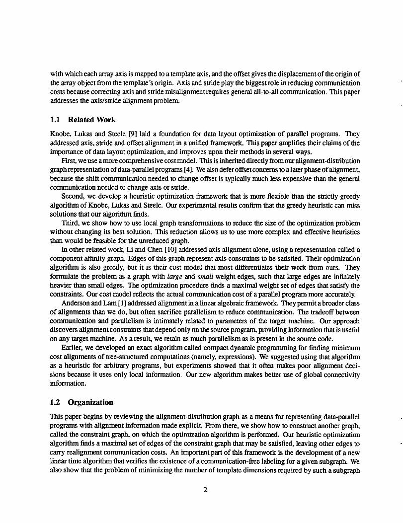
Figure 1: A code fragment using reduce and spread and its ADG. Data weights on edges represent the

cost of communication. Each port has a position label. The ADG represents data flow in a program. It can

also include nodes that reflect control flow due to branches or loops.

is NP-complete. Concluding sections compare this approach to others and summarize test results conducted

with an implementation of the algorithm described.

2 Representing the Alignment Problem

Previously, we developed a representation of data-parallel programs called the alignment-distribution graph

(ADG) [4] to evaluate data layout decisions made during compilation. The ADG is based on static single

assignment form [5], but incorporates a "position semantics" that makes each communication operation of

the program explicit. This section shows how to distill the ADG to a simpler graph that only represents axisand snide.

2.1 The Alignment-Distribution Graph

An example ADG for a Fortran 90 code fragment appears in Figure 1. Nodes in the graph represent

computation, and edges represent flow of data. An endpoint of an edge is called a port and represents

an array object with a specified position. Thus, an edge transforms an array object from one position

to another. Realignment occurs whenever the two ports of an edge have different positions. A node

constrains the relative positions of its ports, which are the locations of its operands and results. For example,

the elementwise MULTIPLY node in the figure requires that its arguments and result ports be aligned

identically. In the figure, positions are represented as the matrices, Ll, L2 and L3. These are described next.

A position is an affine mapping from the coordinates of an array object of d dimensions to the coordinatesof the template of t dimensions. An array point Pa 6 7 a is mapped to a template location Pt 6 Z t by the

followingmatrixequation:pt = L pa + f,

where L is an t x d matrix of integers and f is a column vector specifying the offset component of the

mapping. Here, we consider only axis and stride alignment, so the offset component becomes zero. Thus, a

position is completely determined by the array L. For example, the two-dimensional object A with position

Ll= 0 00 3

is mapped to a three-dimensional template with its first axis mapped to the first axis of the template with

stride 2, and its second axis mapped onto the third axis of the template with stride 3.

Suppose axis j of an array object is mapped to axis i of the template with stride s. Then column j of

the object's position matrix has exactly one nonzero element, in row i, with value s. Row i has no other

nonzeros, because at most one array axis maps to each template axis. We call a matrix with exactly onenonzero in each column and at most one nonzero in each row a D-matr/x.

The data weight of the edge is the total amount of data it transfers. If the endpoints of an edge have

different positions, the edge incurs communication cost equal to its data weight. (Our experiments in

Section 5 indicate that this "discrete metric" is a good model of axis/stride realignment cost; the ADG

framework can support other cost metrics as well [4].)

The total cost of an assignment of positions to ADG ports is the sum of the data weights on edges whose

endpoints are at different positions. In ADG terms, the objective of alignment is to find an assignment ofpositions that minimizes this cost.

2.2 The Constraint Graph

The ADG represents alignment and distribution for arrays in a parallel program. In this section, we transform

the ADG into a simpler graph, called the constraint graph (CG), that is specific to alignment analysis. The

CG unifies the representations of positions and constraints, and effcienfly captures the costs associated with

each constraint. Each port in the ADG becomes a vertex in the CG. Edges and nodes in the ADG contribute

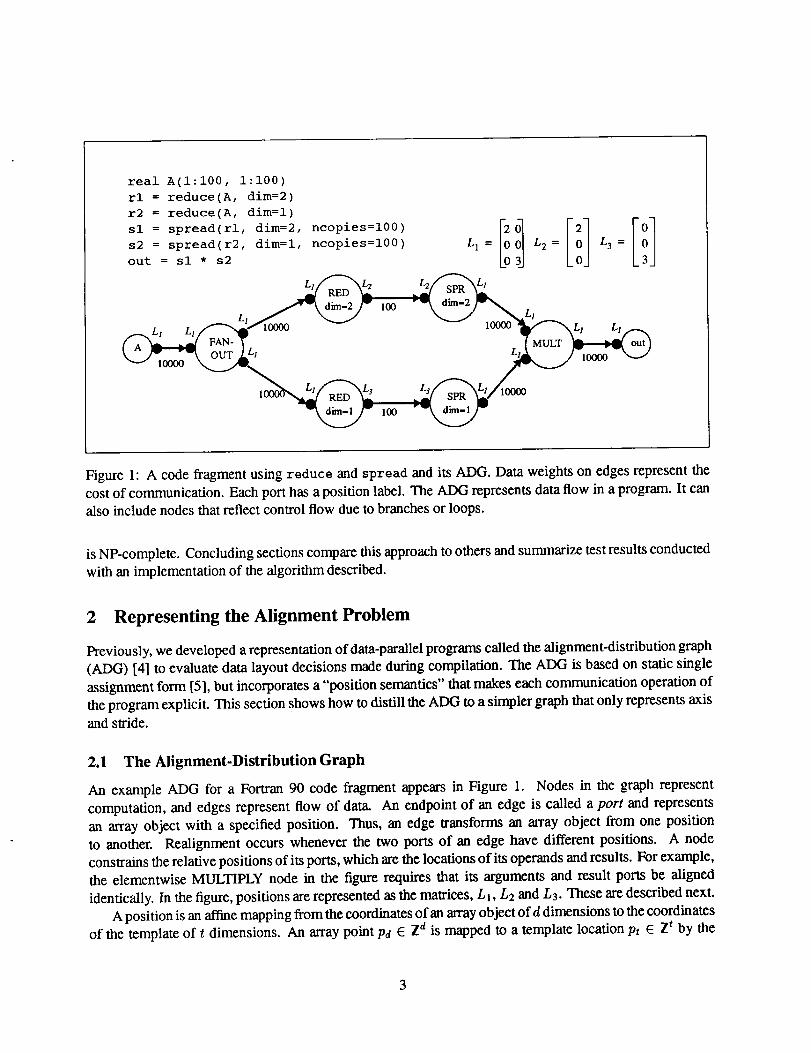
constraints, which are represented as edges in the CG. Figure 2 illustrates the transformation of a line of

source code into an ADG node and then into a CG, with positions and constraints given as matrices. Therest of this section describes the construction and use of the CG.

An ADG node imposes a constraint on the positions of its ports that cannot be violated. A constraint is

a mapping from the coordinate space of one array object to another. If a node involves two array objects, x

and y, and imposes a constraint on the position of V with respect to x, then this constraint can be written as

Lv = L:_Cxv,

where C_ is a constraint matrix. A constraint matrix is a D-matrix having at least as many rows as columns.

Because both Lx and L_ describe mappings to the template, this equation says that corresponding

elements from the two array objects are mapped to the same template site. For a node involving three

or more ports, one is designated the reference port, and the constraints arc expressed relative to it. The

construction of constraint matrices for the various node types of the ADG is sWaighfforward [4].

An ADG edge between two ports, x and y, imposes an equality constraint that may be violated at a

specified cost, Wx_. We write such as constraint in the same form

Ly = LxC::v,

sl=spread(rl,dim=2,ncopies=lO0)

E'] ILl

100 _i oo ,7" 10000

[1oO.........Eo ]O

Figure 2: A code fragment, its translation into an ADG node, and the resulting constraint graph. Each

port has a position (shown below) and each edge imposes a constraint (shown above). A position labeling

satisfies an edge if the head position is the product of the tail position and edge constraint.

where in this case Cxy is an identity matrix. Positions matrices are D-matrices, and it turns out that constraintmatrices are also D-matrices.

The CG is constructed from these constraints. For each array object z, (that is, each ADG port), there

is a vertex vx. For each constraint Lu = L_C_y, there is a directed edge from v_: to vu with label C_ u.

Each edge also has an associated weight W_ u, which is the communication cost of moving an object from

position L_ to L_ if the constraint is not satisfied. An edge in the CG that corresponds to a node constraint

in the ADG has W_ u = _.A labeling of the CG is called "communication-free" if it satisfies every edge constraint, and a CG is

called "satisfiable" if at least one such labeling exists.

This simple formulation captures all of the possible constraints pertinent to alignment analysis among

array objects in High Performance Fortran. For example, constraint matrices can express relations between

arrays that are projections, reductions or sections of one another. The CG may be simplified even further.

Section 4 discusses graph contraction operations that often reduce an alignment problem to a graph of onlya few vertices.

3 An Axis/Stride Labeling Algorithm

The alignment problem is surprisingly hard. It is NP-complete even when restricted to only axis alignment

for two-dimensional arrays in a two-dimensional template. Thus, we must be satisfied with heuristic or

approximate solutions.

Theorem 1 Min-cost labeling of an ADG is NP-complete, even considering only straight-line programs

involving two-dimensional arrays with the transpose and addition operations.

Proof: It is easy to see that min-cost labeling is in NP since the cost of a given axis labeling can be

computed in polynomial time. We proceed by reduction from "Bipartite Subgraph (GT25)", [6] which is

the following problem: Given a graph G and an integer k, is there a bipartite subgraph of G with at least k

edges? (Equivalently, is there a way to 2-color the nodes of G that violates the color condition for at most

t = e - k edges?) This is NP-complete even if G has only vertices of degree 2 and 3.

Wefirsf transform G to a graph with two kinds of edges, "opposite" edges whose endpoints are to be

colored differently and "same" edges whose endpoints are to be colored the same. Each original edge of G

is an "opposite" edge. Split each degree-2 node of G into two nodes joined by a new "same" edge. Split

each degree-3 node of G into a 4-vertex star, each of whose leaves is incident on an original edge, with 3

new "same" edges. It is easy to see that G can be 2-colored in a way that violates at most t edges if and only

if the transformed graph can be. Furthermore, since each "opposite" edge shares a degree-2 endpoint with

a "same" edge, the transformed graph has an optimal 2-coloring that violates only "same" edges.

Now each degree-2 vertex is incident on one "opposite" edge and one "same" edge, and each degree-3

vertex is incident on three "same" edges. Construct an ADG by replacing each "opposite" edge and its

two endpoint vertices with a transpose node, and replacing each degree-3 vertex with an addition node.

(Formally, replace each degree-3 vertex with a node, then direct the edges so no degree-3 node is a source

or a sink, then make the ones with in-degree 2 addition nodes.) Each edge of the ADG is a "same" edge of

the transformed graph. Each "opposite" edge of the transformed graph (i.e. each edge of the original graph)

is a transpose node of the ADG. A min-cost labeling of the ADG corresponds to an optimal 2-coloring of

the transformed graph that violates only "same" edges.[]

3.1 Outline of the Algorithm

Let G be a given CG. Like the greedy algorithms of Knobe, Lukas and Steele [9] and Li and Chen [10], our

algorithm finds a maximal satisfiable subgraph of G. Our algorithm is not strictly greedy--it can discard

edges as well as add them, and therefore will ordinarily explore a larger set of feasible solutions.

Our algorithm builds a maximal satisfiable subgraph G'. Initially G' contains all of the vertices of G,

but all edges are excluded. At each step, an excluded edge is conditionally added to G' and a subroutine

is-satisfiable determines if there exists a communication-free labeling for the augmented graph G _.

The optimization algorithm proceeds as follows:

1. Include an excluded edge.

. If the resulting graph is satisfiable (see Section 3.2) then accept the new edge and go to Step 1.

Else, find a minimum-weight cut set E in G' of edges between the endpoints of the edge e. The graph

including e but with E removed is guaranteed to be satisfiable (see below). However, there may be

edges in E whose inclusion does not prohibit satisfiability. Try including each edge in E back into

the graph in turn, and retain in E only those edges that prohibit satisfiability. E is now a minimal set

of edges whose removal allows a communication-free labeling of the graph with edge e.

3. If the weight of edge e is bigger than the total weight of edge set E then insert e in the graph and

move the edges in E into the bag. Otherwise, reject e and leave the graph as it was.

4. Repeat this procedure until no edges from the bag can be added into the graph.

5. Find a labeling thatsatisfies the final graph (see Section 3.3).

The procedure terminates because the weight of the current graph increases at every iteration (though

its size may no0.

Lemma 1 In step 2, the graph with e included and E removed is satisfiable.

6

PI w,3x,1 y, z,w x y z w_

vW yqlw I'_

(2-D) (2-D) (2-D) (l-D)

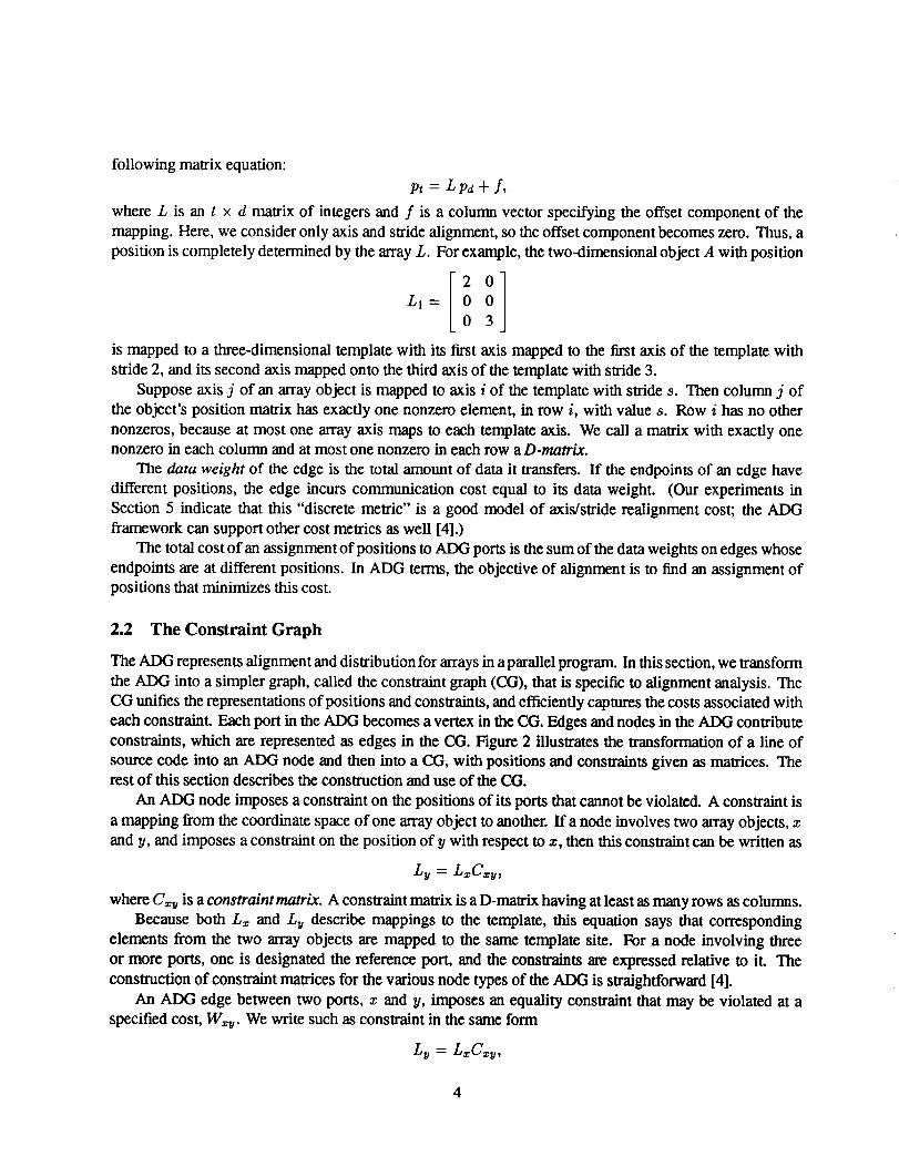
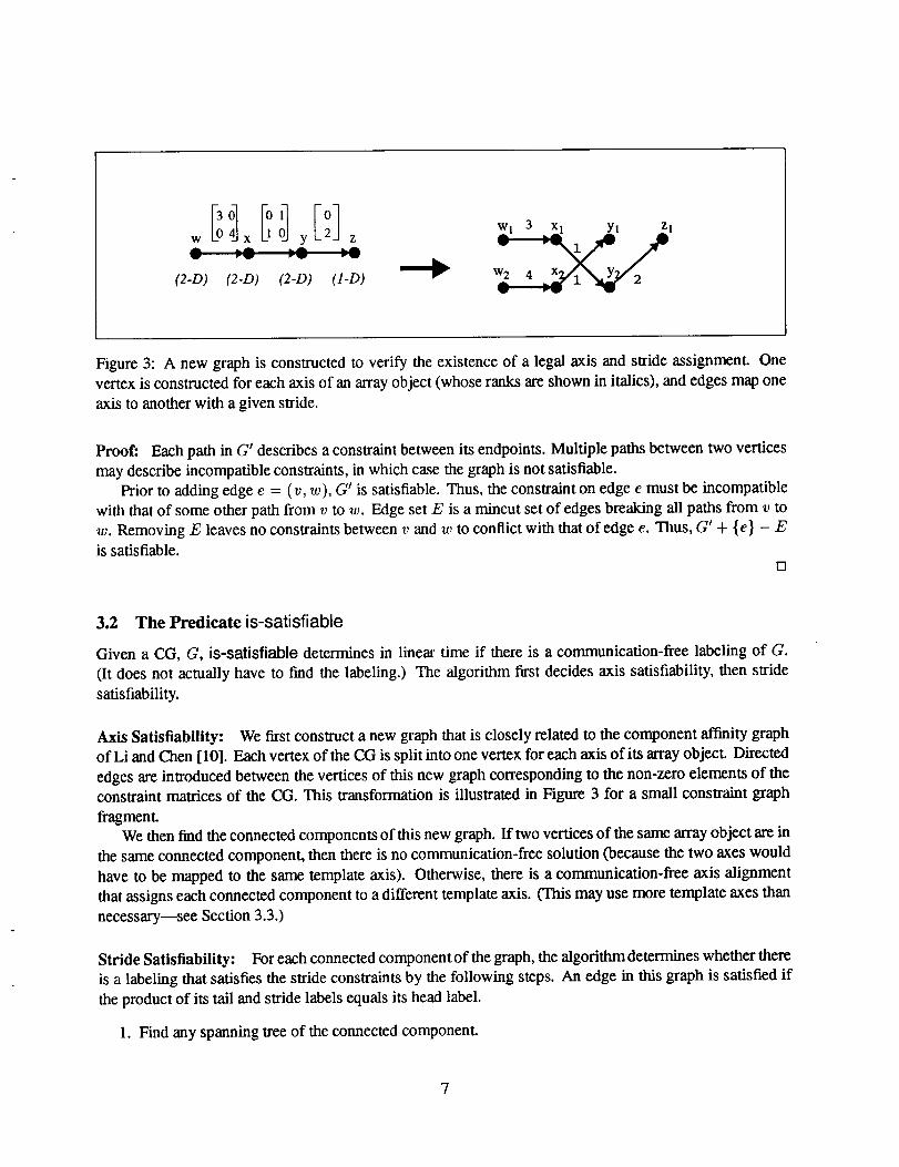
Figure 3: A new graph is constructed to verify the existence of a legal axis and stride assignment. One

vertex is constructed for each axis of an array object (whose ranks are shown in italics), and edges map one

axis to another with a given stride.

Proof: Each path in G' describes a constraint between its endpoints. Multiple paths between two vertices

may describe incompatible constraints, in which case the graph is not satisfiable.

Prior to adding edge e = (v, w), G' is satisfiable. Thus, the constraint on edge e must be incompatible

with that of some other path from v to w. Edge set E is a mincut set of edges breaking all paths from v to

w. Removing E leaves no constraints between v and w to conflict with that of edge e. Thus, G' + {e} - E

is satisfiable.[]

3.2 The Predicate is-satisfiable

Given a CG, G, is-satisfiable determines in linear time if there is a communication-free labeling of G.

(It does not actually have to find the labeling.) The algorithm first decides axis satisfiability, then stride

satisfiability.

Axis Satisfiability: We first construct a new graph that is closely related to the component affinity graph

of Li and Chen [10]. Each vertex of the CG is split into one vertex for each axis of its array objecL Directed

edges are introduced between the vertices of this new graph corresponding to the non-zero elements of theconstraint matrices of the CG. This transformation is illustrated in Figure 3 for a small constraint graph

fragment.We then find the connected components of this new graph. If two vertices of the same array object are in

the same connected component, then there is no communication-free solution (because the two axes would

have to be mapped to the same template axis). Otherwise, there is a communication-free axis alignment

that assigns each connected component to a different template axis. (This may use more template axes than

necessary--see Section 3.3.)

Stride Satisfiability: For each connected component of the graph, the algorithm determines whether there

is a labeling that satisfies the stride constraints by the following steps. An edge in this graph is satisfied if

the product of its tail and stride labels equals its head label.

1. Find any spanning tree of the connected component.

2. Labelanarbitraryvertex"1" andlabel the rest of the vertices by multiplying (or dividing) by the

stride label of the edges.

3. For each non-tree edge, check whether the stride transformation it describes is satisfied by its endpoints.

The running times of both the axis and stride phases of this algorithm are linear in the number of edges in

the graph. Connected components can be found in linear time by a depth first search. Checking the vertices

corresponding to each array object to determine if any are in the same component is trivial. The stride

constraints can be verified during the depth-first search: as each node is visited, propagate the appropriate

stride value to each non-visited neighbor. For all other neighbors, verify that the constraint on the edge issatisfied.

This algorithm performs operations similar to the conformance checking procedure of Knobe, Lukas

and Steele [9], but is much simpler. They find axis conflicts by an incremental approach based on merging

sets and their stride satisfiability test involves complicated array allocation functions. These differences

stem from the differences in the two optimization frameworks. Our approach can generate large-scale

changes to the constraint graph, requiring that we recompute satisfiability anew each time. For this reason,

we developed the efficient linear-time algorithm given here. In contrast, they considered the addition of

only a single edge at each step, and incremental techniques were more appropriate.

3.3 Providing a Labeling

The is-satisfiable procedure implicitly finds an axis and stride labeling, but its axis labeling may use more

template axes than necessary. When the final maximal satisfiable subgraph is found, we label the axes by a

coloring procedure as follows.

We construct another graph to describe the coloring problem: the axis quotient graph. This graph has

one vertex for each connected component of the axis/stride satisfiability graph, and an undirected edge

between vertices representing two connected components that occur in the same array object. A k-coloring

of this graph corresponds to an assignment of the axes of each array object to k template axes. Each color

corresponds to an axis of the template, and a k-coloring of the graph assigns the axes of each array object

to different axes of the template. Finding an optimal coloring is hard:

Theorem 2 Given an ADG that admits a communication-free labeling, axis assignment to minimize the

number of template dimensions is NP-complete.

Proof: It is easy to see that this problem is in NP since we can use procedure is-satisfiable to verify

the validity of a given axis alignment in polynomial time. We proceed by reduction from "Graph k-

colorability (GT4)" [6] which is the fonowing: Given a graph G = (V, E) and a positive integer k < IVI,

is G k-colorable, i.e., does there exist a function f : V --, { 1,2,..., k} such that f(u) # f(v) whenever

{u, v} E E? This is solvable in polynomial time for k = 2, but remains NP-complete for all fixed k E 3.

Given an instance of GT4, we reduce it to an instance of our problem as follows.

• For each vertex vi of G, construct an input node in the ADG for a variable called tl of dimension(I:N).

• For each edge e,-,,, construct an input node in the ADG for a two-dimensional array called A,,, with

dimensions (1 : N, 1 : N).

For each edge em= (i, j), construct two ADG section assignment nodes that express:

Am(:, 1) = ti

Am(l,:) = tj.

Claim: For any k < IVI, the ADG has an axis assignment with k template dimensions iff graph G isk-colorable.

Let each color correspond to a template dimension, and k be the dimensionality of the template. Each

array ti is assigned to dimension f(vi) ill the template, and each array Am spans two dimensions in the

template: the dimensions f(vi) and f(vj ).

(IF) Assume that G is k-colorable, then the mapping described above yields an assignment of template

dimensions to array axes that does not violate the constraint that the axes of a given object must lie in

different template dimensions.

(ONLY IF) Assume that the ADG has a legal assignment of axes to template dimensions and the mapping

described above is constructed. Then the assignment does not violate the constraints of the colorability

problem that the endpoints of each edge must have different colors.[]

In practice, however, the axis quotient graph is usually easy to color and standard heuristics [2] find an

optimal coloring.

4 Contracting the Constraint Graph

The constraint graph may be contracted into a smaller graph that captures all of the alignment constraints

and costs of the original graph. We can then use the algorithm of Section 3, or any other method, to align

the contracted graph, and propagate the results back to the original graph by reversing the contractions. For

many examples, the contracted constraint graph has only a few vertices. Since performing the contractions

is inexpensive compared to doing the alignment, contraction makes the total running time much smaller.

4.1 Contraction Operations

The contractions rely on the following property of D-matrices.

Lemma 2 Let Y and C be given D-matrices. There is always at least one D-matrix X such that X C = Y.

Proof: Let X be a (p x q) matrix, C be (q x r), and Y be (p x r). Without loss of generality, the rows

and colunms of the matrices may be permuted to place C in upper diagonal form. Now, if q = r, then C

is a diagonal matrix and X is uniquely determined. Otherwise, q > r and the problem may be written asfollows:

0 "

D is a nonsingular (r x r) matrix, Xl is (p x r) and X2 is (p x (q - r)). Matrix Xl is fully specified by

Y and D. Any value for X2 satisfies the equation, but it must be chosen so that X is a D-matrix, which

is simple. The r columns of X1 are multiples of r standard basis vectors {el, e2,'.., ep}. The (q - r)

columns of 2(2 must be multiples of the remainder and there are (p - r) such columns remaining. Since

(p >_ q), there is at least one way in which this can be achieved. []

We now present four situations where the CG can be contracted.

9

Contraction 1: Suppose vertex v has degree 1, so v is adjacent to only one other vertex w. The edge

between them has a directed constraint C,,,_ or Cwv. In either case, contract the graph G into a smaller graph

G' by removing v and the edge. To convert an alignment for G' into one for G with the same cost, choose

a position P, for v as follows. If the edge was directed (w, v), then compute P_ = P,_C_,,_. If the edge was

directed (v, w), solve PvC,,w = P_, for Pv by Lemma 2.

Contraction 2" The second contraction applies when a vertex v is adjacent to only two different vertices.

In this case there is an edge (u, v) and an edge (v, w), and u _ v _ w _ u. Construct G j by eliminating

v and contracting the two edges into a new edge (u, w) with edge label C_,,_ = C,_vC_,_o, and weight

W,_o = min(W,,,,, W,_,,,). To convert an alignment for G' into one for G with the same cost, choose a

position for v as follows.

There are two cases. If the alignment for G' satisfies edge (u, w), then compute P_ = P,,C,,,,. This

satisfies (u, v) in G, and (v, w) is also satisfied because P_o = P,_C_,_ = P_,C,,,_C_,_o = P_,C_,_. If the

alignment for G' does not satisfy (u, w), then (u, w) contributes cost W,,,, = min(W,,,,, W,,_o) to G'. We can

construct an alignment for G with the same cost by falling to satisfy the less expensive of (u, v) and (zt, w):

If W_,, < 14ruvthen let Pv = P_,C_,_, and if W,,_ < W_ the solve Pw = P_C_w for P_ by Lemma 2.

Contractions 3 and 4: There are two final contraction operations. Merge parallel edges if their constraint

matrices are equal and add their edge weights. Finally, reverse edges with invertible constraints. (Note that

all square D-matrices are invertible.) This may enable other contraction operations.

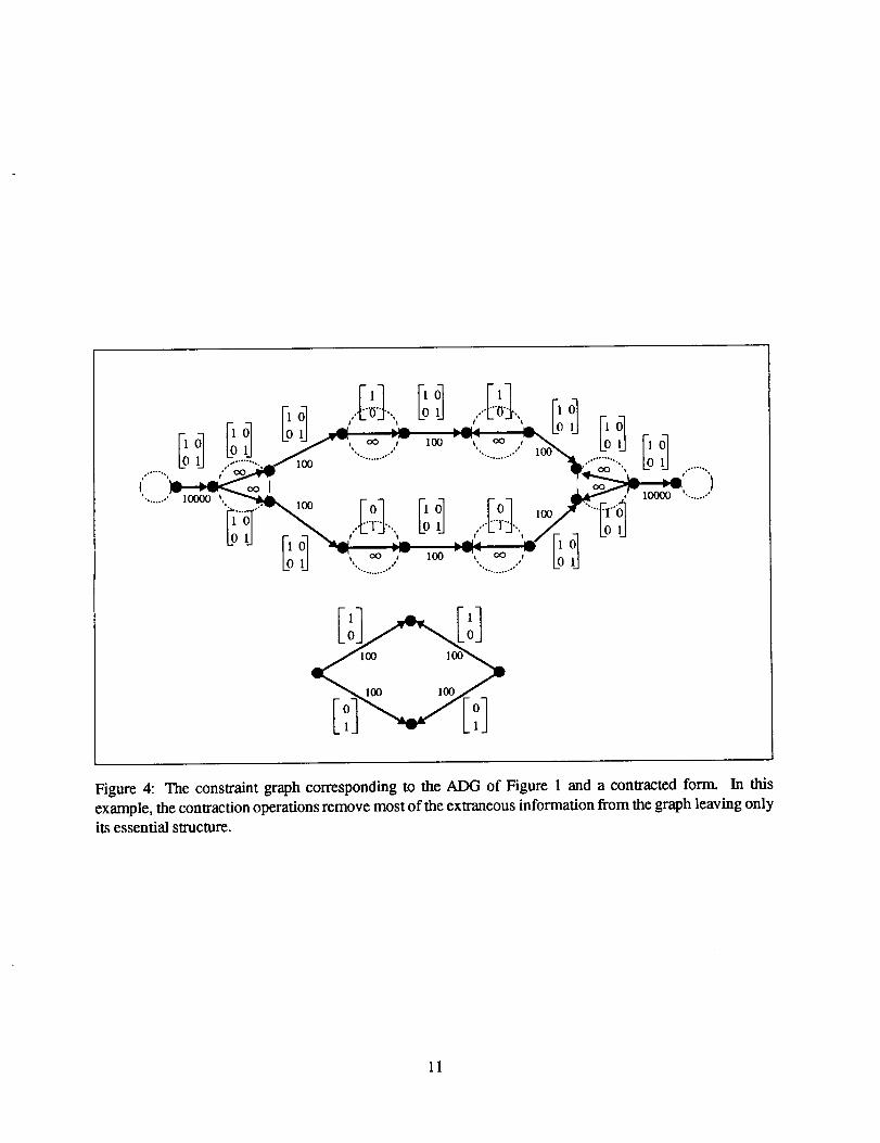
Figure 4 illustrates these contraction operations. The initial constraint graph corresponds to the example

program and ADG of Figure 1. Contraction eliminates dangling acyclic branches and combines edges in

series. The result is a very simple graph capturing the essential structure of the problem.

5 Experimental Results

To illustrate our algorithm, we constructed the two small example programs shown in Figure 5, which have

nontrivial axis alignment issues.

We generated alignments for the programs using our algorithms with various edge selection rules and

ran the optimized programs on the CM-5 to measure the effect of alignment on their running times. Because

the CMF compiler does not allow axis-changing alignments [11], we broke alignment into two parts. We

performed axis alignment manually by changing the orientation of the arrays in the program and including

explicit array transpose operations for unsatisfied CG edges. We specified stride alignment by addingALIGN directives to the source code.

We did three kinds of experiments. First, we examined the effect of edge selection strategy on the

quality of solutions found. Second, we examined the effect of axis and stride alignment on running time,

and the correlation between the discrete metric of the optimization problem and the actual running time on

10

......Lo_ ,.:..__,oo ........................ F'°l

' '_l_ _ ,' lO000 %......°

IL.°1 \ ,,..h.:j..,,,..,_-.{[rJ"'_-"{F,a hodLOU F1 ol "'_, _9Log ,,...._....,,,oo-,,...._....,, Lod

0 0[:]v[l

Figure 4: The constraint graph corresponding to the ADG of Figure 1 and a contracted form. In this

example, the contraction operations remove most of the extraneous information from the graph leaving only

its essential structure.

11

PROGRAM program1

REAL, ARRAY(IO00, I000) :: A, B

C=A+B

B(1:800,I:800) = A(1:800,I:800) - transpose(B(l:800,1:800))

A(1:800,1:800) = transpose(A(1:800,1:800)) - B(1:800,1:800)

END PROGRAM

PROGRAM program2

PARAMETER(N=IO00)

REAL, ARRAY(N, N) :: A, B

SUM = A + transpose(B)

DIFF = transpose(A) - B

A2 = SUM(I:N/2, I:N/2)

B2 = DIFF(I:N/2, I:N/2)

HALFSUM = A2 + B2

HALFDIFF = A2 - B2

AS = HALFSUM(I:N/4, I:N/4)

B3 = HALFDIFF(I:N/4, 1:N/4)

QUARTSUM = A3 + transpose(B3)

QUARTDIFF = transpose(A3) - B3

A(I:N/4, 1:N/4) = transpose(QUARTSUM)

B(I:N/4, I:N/4) = transpose(QUARTDIFF)

AVG = (A + B) / 2.0

END PROGRAM

Figure 5: Two example programs.

12

Table 1: The estimated and actual times of two programs under differing axis and

Example Method Communication CM5 runningCost time (secs)

PROGRAM 1

PROGRAM2

(none)

max-wt

min-wt

random

(optimal)

(none)

max-wt

min-wt

random

(optimal)

128O00O

1000000

1280000

1000000

1750000

1375000

1312500

1312500

.25

.25

.13

.25

.13

.62

.56

.40

.34

.34

stride alignments.

the CM-5. Third, we examined the effect of graph contraction on the time required to find a solution.

5.1 Edge Selection Ordering

At each iteration the optimization algorithm removes an edge from the bag. We examined three edge selection

strategies: maximum weight first, minimum weight first and random selection. With the maximum weight

ordering, our algorithm reduces to the greedy heuristic proposed by Knobe, Lukas and Steele. However, our

experimental results show that other orderings (combined with the min-cut procedure) can yield superiorresults.

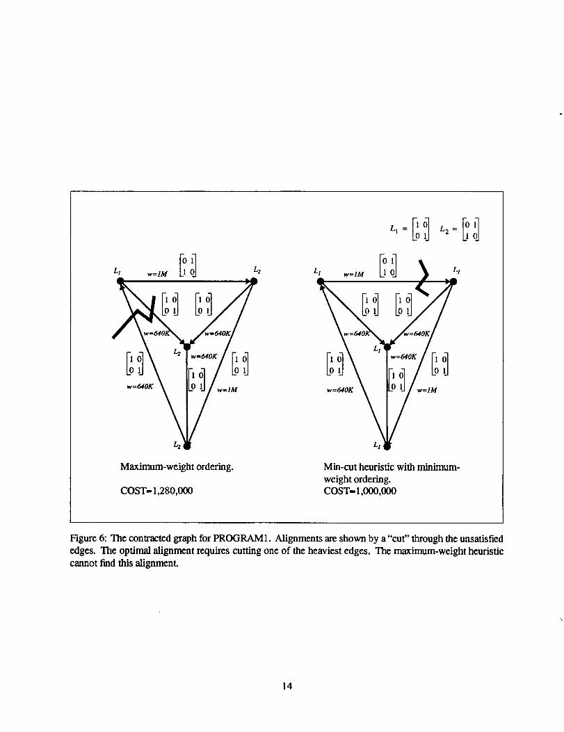
The contracted graph for PROGRAM 1 appears in Figure 6 with two different alignments. One requires

communication on two edges, for a total cost of 1,280,000. The optimal solution requires communication

on only one edge and costs 1,000,000. This optimal solution was found using the minimum edge-weight

heuristic and the min-cut procedure. This example demonstrates a shortcoming of the maximum-weight

heuristic: the optimal solution in this example cannot be found if edges are added in order of decreasing

weight, because the subgraph of heaviest edges is satisfiable, but not optimal.

5.2 Execution Time

We measured the execution time of each of the programs on the CM-5 with each alignment our algorithm

generated, and also without axis or stride optimization as a baseline. The times measured were averagedover ten runs. Table 1 presents the data. The solution reported for the random edge selection heuristic

reflects the best of five trials. The table shows the estimated cost according to the discrete metric and the

actual execution time of the program.We draw two conclusions. First, optimizing axis and stride alignment can significantly improve the

running time of the programs. Second, our discrete metric of communication cost is an accurate enough

measure to correctly predict the relative running times with different alignments.

13

L1 w--IM _ L1

A

Maximum-weight ordering. Min-cut heuristic with minimum-

weight ordering.COST= 1,280,000 COST= 1,000,000

Figure 6: The contracted graph for PROGRAM1. Alignments are shown by a "cut" through the unsatisfied

edges. The optimal alignment requires cutting one of the heaviest edges. The maximum-weight heuristic

cannot find this alignment.

14

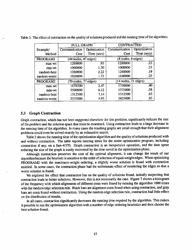
Table2:Theeffectofcontractiononthe quality of solutions produced and the running time of the algorithm.

Example/Method

FULL GRAPH

Communication Optimization

Cost Time (secs)

CONTRACTED

Communication Optimization

Cost Time (sees)

PROGRAM 1 (44 nodes, 47 edges) (4 nodes, 6 edges).95

1.50

2.22

1.72

1280000

1280000

1640000

max-wt

min-wt

random-best

random-worst

1280000

1000000

1280000

1920000

PROGRAM2 (70 nodes, 77 edges) (14 nodes, 21 edges)

max-wt

min-wt

random-best

random-worst

1750000

1375000

1312500

2625000

1678500

2500000

1312500

2375000

2.47

6.12

7.14

4.93

.23

.23

.19

.25

.40

.58

.63

.65

5.3 Graph Contraction

Graph contraction, which has not been suggested elsewhere for this problem, significantly reduces the size

of the problem and the solution space that must be examined. Using contraction leads to a large decrease in

the running time of the algorithm. In many cases the resulting graphs are small enough that their alignment

problems could even be solved exactly by an exhaustive search.

Table 2 shows the running time of the optimization algorithm and the quality of solutions produced with

and without contraction. The table reports running times for the entire optimization program, including

contraction if any, on a Sun-4/370. Graph contraction is an inexpensive operation, and the time spent

reducing the size of the graph is easily recovered by the time saved in the optimization phase.

Although contraction preserves the cost of the optimal alignment, it can change the result of our

algorithm because the heuristic is sensitive to the order of selection of equal-weight edges. When optimizing

PROGRAM2 with the maximum-weight ordering, a slightly worse solution is found with contraction

enabled. In some cases, the contraction phase had the unfortunate effect of reordering the edges so that a

worse solution is found.

We explored the effect that contraction has on the quality of solutions found, initially suspecting thatcontraction leads to better solutions. However, this is not necessarily the case. Figure 7 shows a histogram

of the frequency with which alignments of different costs were found by running the algorithm 1000 times

with the random edge selection rule. Black bars are alignment costs found when using contraction, and gray

bars are costs found without contraction. Using the random edge selection rule, contraction had little effect

on the distribution of results.

In all cases, contraction significantly decreases the running time required by the algorithm. This makes

it possible to run the optimization algorithm with a number of edge ordering heuristics and then choose thebest solution found.

15

70G

60G

50Q

30¢

20G

10¢

Effect of Conlzac_n on Program 1 AIIgnrnents Effect of Contraction on Program 2 Aligrcrtw_4501

4001

_01

3001

2SOl

2001

1501

1001

SOl

O',; 1'.4 ,_ 18 '_2,4 2.6 2.8

Communication Cost x 10e x 10a

1.4 1.6 t .8 2 2.2Commu_cat_n C_

Figure 7: The effect of contraction on the quality of solutions found over 1000 runs of the algorithm using

the random edge selection rule. Black bars show alignment costs found when using contraction; gray bars

show costs found without contraction. Surprisingly, the distribution of results found is unchanged whencontraction is used.

6 Conclusions

This paper presents a new approach m axis and stride alignment to optimize array placement in data-parallel

programs. Our algorithms extend those previously reported in a number of ways.

Our algorithms use a problem formulation based on the ADG representation. The ADG makes explicit

all array objects generated by a program--named arrays as well as unnamed temporaries. Thus, the

optimization algorithm has complete control over the placement of every array generated. The ADG also

incorporates the effects of control flow into its data flow representation; this information can affect alignment

decisions. Other work has not treated control flow as completely.

The graph contraction operations greatly reduce the computation time of the program. For many

examples, the contracted constraint graph becomes a graph of only a few vertices, and the alignment

problem can be solved exactly. Even when an exact method is not feasible, the reduced size of the

contracted graph makes possible a more complete search of the space of possible solutions. We believe

that even more powerful graph contractions are possible; indeed we hope eventually to define a set of

contractions that reduces most programs enough that optimal alignments can be found by an exponential

search procedure.

Axis and stride alignment is a discrete optimization problem. The optimization algorithm we propose is

actually a family of optimization algorithms parameterized by an edge ordering. For one particular ordering,

our algorithm reduces to the algorithm of Knobe, Lukas and Steele. However, we have shown that other

orders, coupled with the min-cut procedure, can lead to superior solutions. Edge orderings based on graph

structure may be possible, and there may be more efficient means of finding conflicting edge sets. We intend

to investigate these issues in the future.

16

Acknowledgements

David Bau and Lenny Oliker implemented an earlier version of the axis, stride, and offset alignment

algorithms, and our experiments here are built on their testbed. The proof of Theorem 1 is also due to David

Bau. We thank both of them as well as Jingke Li and Shang-Hua Teng for stimulating discussions of all

these problems.

References

[1]

[2]

[31

Jennifer M. Anderson and Monica S. Lam. Global optimizations for parallelism and locality on scalable

parallel machines. In Proceedings of the ACM SIGPLAN'93 Conference on Programming Language

Design and Implementation, pages 112-125, Albuquerque, NM, June 1993.

Gregory J. Chaitin, Marc A. Auslander, Ashok K. Chandra, John Cocke, Martin E. Hopkins, and

Peter W. Markstein. Register allocation via coloring. Computer Languages, 6:47-57, 1981.

Siddhartha Chatterjee, John R. Gilbert, and Robert Schreiber. Mobile and replicated alignment of

arrays in data-parallel programs. In Proceedings of Supercomputing'93, pages 420-429, Portland, OR,

November 1993. Also available as RIACS Technical Report 93.08 and Xerox PARC Technical ReportCSL-93-7.

[4]

[5]

[61

[7]

[8]

[9]

[10]

Siddhartha Chatterjee, John R. Gilbert, Robert Schreiber, and Thomas J. ShetIter. Modeling data-

parallel programs with the alignment-distribution graph. Journal of Programming Languages, 1994.

Special issue on compiling and run-time issues for distributed address space machines. To appear.

Ron Cytron, Jeanne Ferrante, Barry K. Rosen, Mark N. Wegman, and E Kenneth Zadeck. Efficiently

computing static single assignment form and the control dependence graph. ACM Transactions on

Programming Languages and Systems, 13(4):451-490, October 1991.

Michael R. Garey and David S. Johnson. Computers and Intractability: A Guide m the Theory of

NP-Completeness. W. H. Freeman and Company, San Francisco, CA, 1979.

High Performance Fortran Forum. High Performance Fortran language specification. Scientific

Programming, 2(1-2): 1-170, 1993.

Kathleen Knobe, Joan D. Lukas, and William J. Dally. Dynamic alignment on distributed memory

systems. In Proceedings of the Third Workshop on Compilers for Parallel Computers, pages 394--404,

Vienna, Austria, July 1992. Austrian Center for Parallel Computation.

Kathleen Knobe, Joan D. Lukas, and Guy L. Steele Jr. Data optimization: Allocation of arrays to reduce

communication on SIMD machines. Journal of Parallel and Distributed Computing, 8(2): 102-118,

February 1990.

Jingke Li and Marina Chen. The data alignment phase in compiling programs for distributed-memory

machines. Journal of Parallel and Distributed Computing, 13(2):213-221, October 1991.

[11] Thinking Machines Corp. CM Fortran User's Guide for the CM-5, version 2.1 edition, January 1994.

17

[12] Skef Wholey. Automatic Data Mapping for Distributed-Memory Parallel Computers. PhD thesis,

School of Computer Science, Carnegie Mellon University, Pittsburgh, PA, May 1991. Available as

Technical Report CMU-CS-91-121.

18