Algoritmi rasterske grafike -...
132
Algoritmi rasterske grafike
Transcript of Algoritmi rasterske grafike -...
Algoritmi rasterske grafike
Risanje primitivov
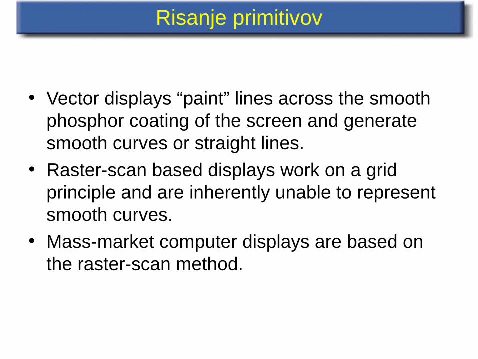
• Vector displays “paint” lines across the smooth phosphor coating of the screen and generate smooth curves or straight lines.
• Raster-scan based displays work on a grid principle and are inherently unable to represent smooth curves.
• Mass-market computer displays are based on the raster-scan method.
Piksel NI majhen kvadrat
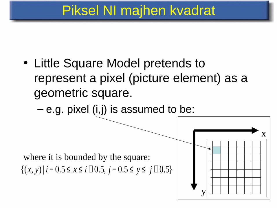
• Little Square Model pretends to represent a pixel (picture element) as a geometric square.– e.g. pixel (i,j) is assumed to be:
x
y
where it is bounded by the square:}5.05.0,5.05.0|),{( +≤≤−+≤≤− jyjixiyx
Piksel NI majhen kvadrat
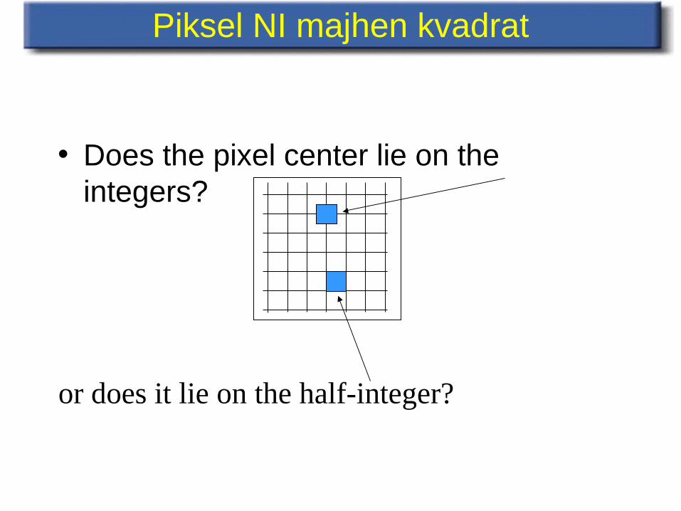
• Does the pixel center lie on the integers?
or does it lie on the half-integer?
Piksel NI majhen kvadrat
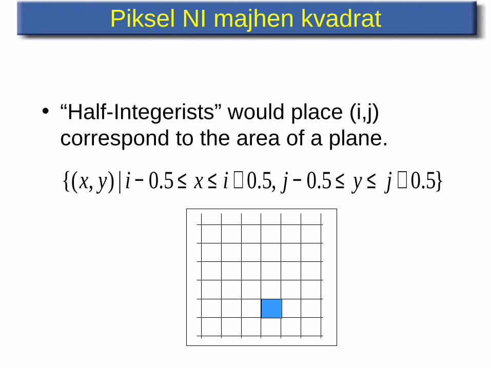
• “Half-Integerists” would place (i,j) correspond to the area of a plane.
}5.05.0,5.05.0|),{( +≤≤−+≤≤− jyjixiyx
Piksel NI majhen kvadrat
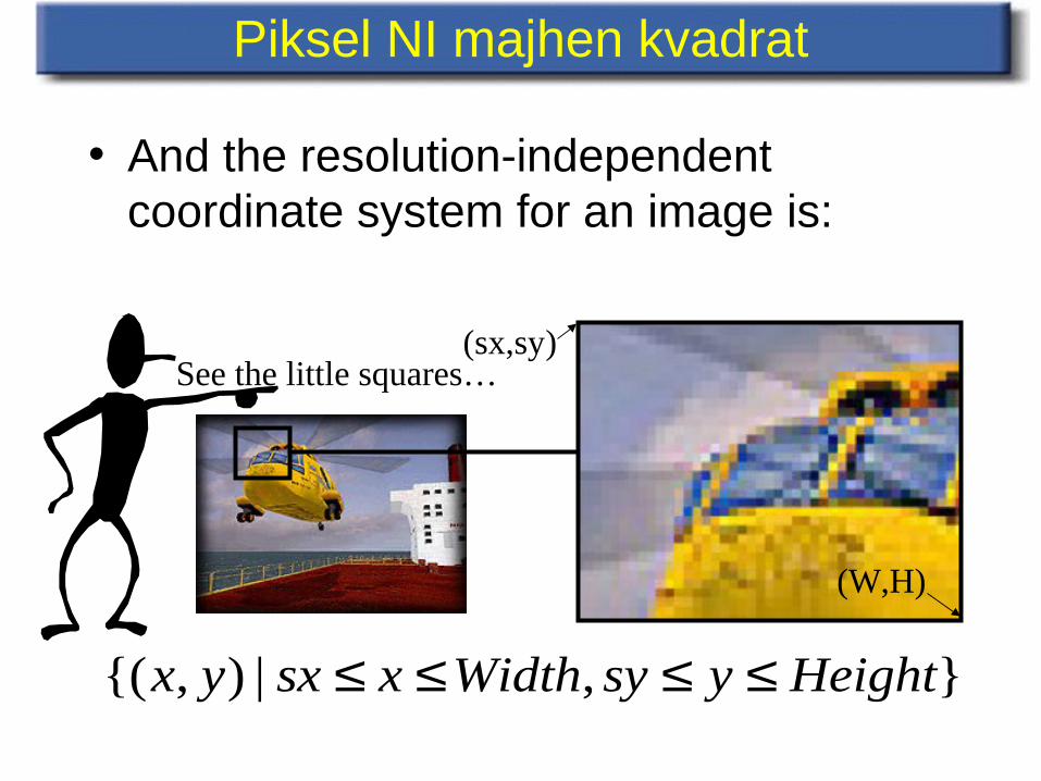
• And the resolution-independent coordinate system for an image is:
},|),{( HeightysyWidthxsxyx ≤≤≤≤
(sx,sy)
(W,H)
See the little squares…
Piksel NI majhen kvadrat
• A pixel is a point sample.
• It only exists at a point.
• A colour pixel will actually contain 3 samples: red, green and blue
• A pixel is not a little square.
• An image is a rectilinear array of point samples (discrete not continuous)
Piksel NI majhen kvadrat
• Why is the “little square model” popular:– Rendering (conversion of abstract
geometry into viewable pixels)
– The mathematics is easier if we assume a continuum.
Piksel NI majhen kvadrat
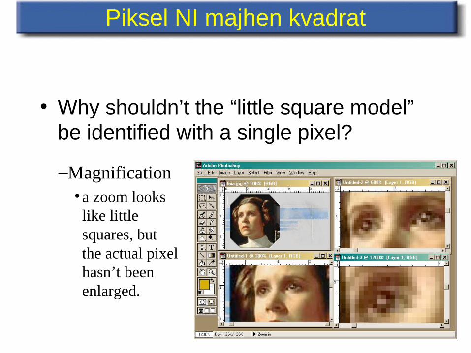
• Why shouldn’t the “little square model” be identified with a single pixel?
–Magnification• a zoom looks like little squares, but the actual pixel hasn’t been enlarged.
Piksel NI majhen kvadrat
• Why shouldn’t the “little square model” be identified with a single pixel?
–Scanner Digitising a Picture–a light source illuminates the paper
–light reflected is collected and measured by a colour sensitive device
–the collected light is passed through a filtering shape (never a square)
–pixels are determined by averaging overlapping shapes.
Uvod v 2D upodabljanje
• 2D primitives – Line segments – Ellipses and circles – Polygons – Curves
• Rasterization (Scan-Conversion) – Turn 2D primitives into sets of pixels – A Pixel Is Not A Little Square (Digital Signal Processing) – Antialiasing
• Clipping – Compute the intersection of a primitive and a shape – Primitive: line segment, polygon – Shape: rectangle, convex polygon
Nekaj matematike
• Coordinate system: y axis upward or downward?
• Pixels are at the centres of integer coordinates
• Line segments – Equation of a (2D) line: ax + by + c = 0
– Direction: (-b a)
– Normal vector: (a b)
– Parametric equation of a segment [P1-P2]x(t) = x1 + t*(x2-x1) = (1-t)*x1 + t*x2y(t) = y1 + t*(y2-y1) = (1-t)*y1 + t*y2t in [0..1]
Nekaj matematike
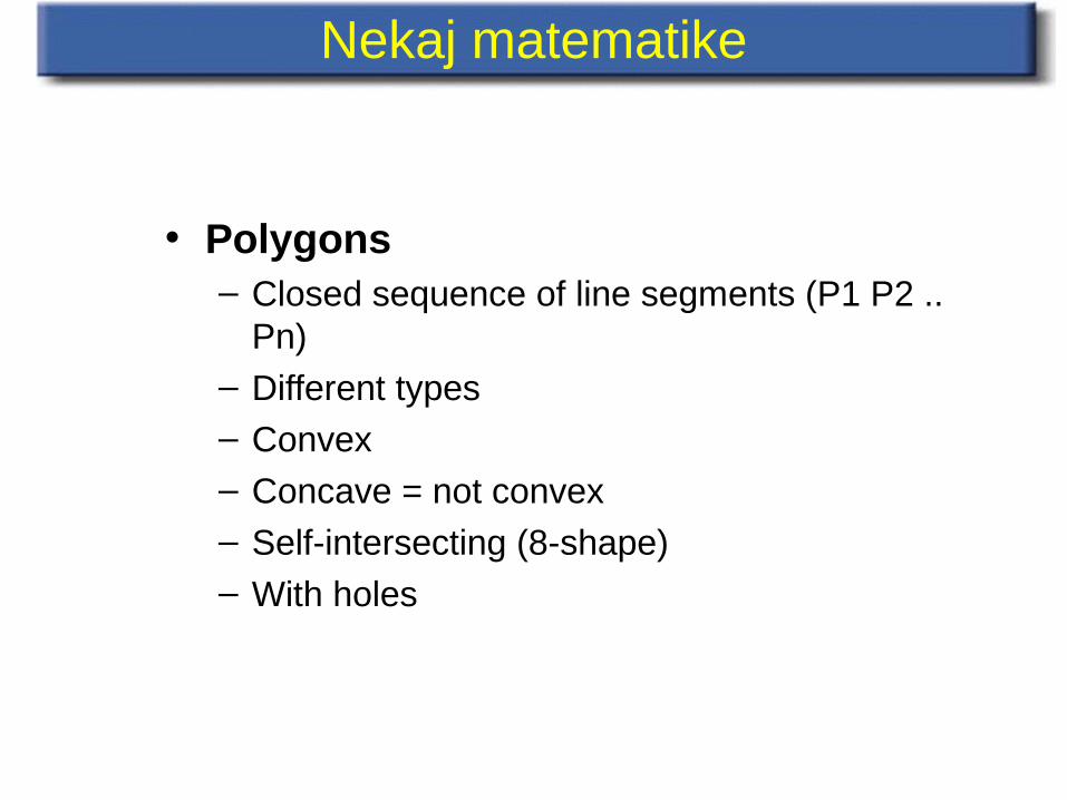
• Polygons – Closed sequence of line segments (P1 P2 ..
Pn) – Different types – Convex
– Concave = not convex
– Self-intersecting (8-shape) – With holes
Rasterizacija
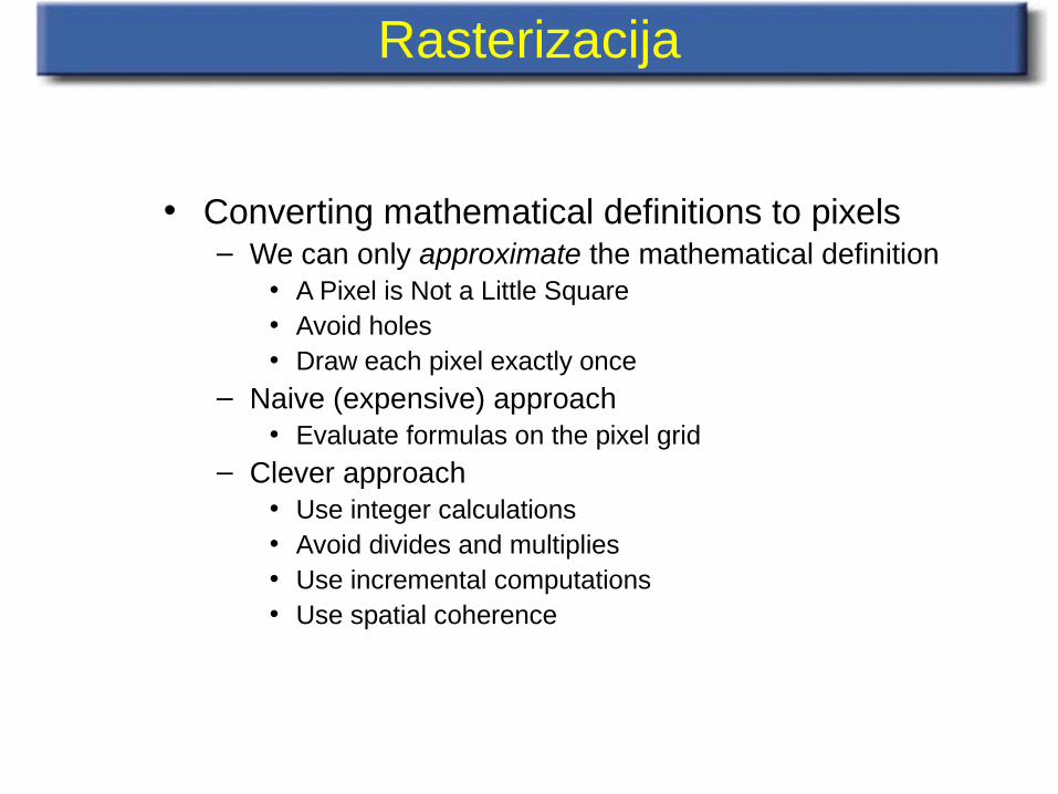
• Converting mathematical definitions to pixels – We can only approximate the mathematical definition
• A Pixel is Not a Little Square • Avoid holes • Draw each pixel exactly once
– Naive (expensive) approach • Evaluate formulas on the pixel grid
– Clever approach • Use integer calculations • Avoid divides and multiplies • Use incremental computations • Use spatial coherence
Ravne črte in krogi
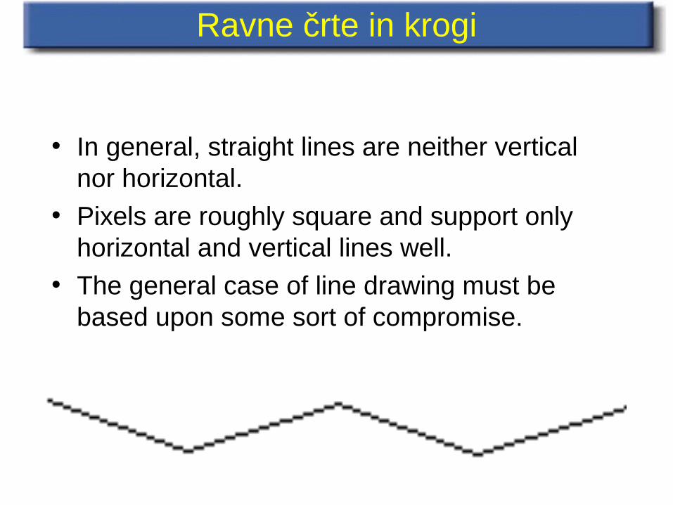
• In general, straight lines are neither vertical nor horizontal.
• Pixels are roughly square and support only horizontal and vertical lines well.
• The general case of line drawing must be based upon some sort of compromise.
Ravne črte
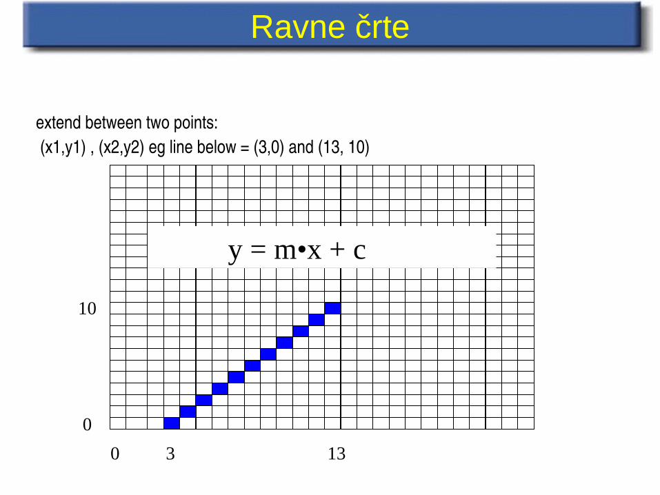
extend between two points: (x1,y1) , (x2,y2) eg line below = (3,0) and (13, 10)
10
0
0 3 13
y = m•x + c
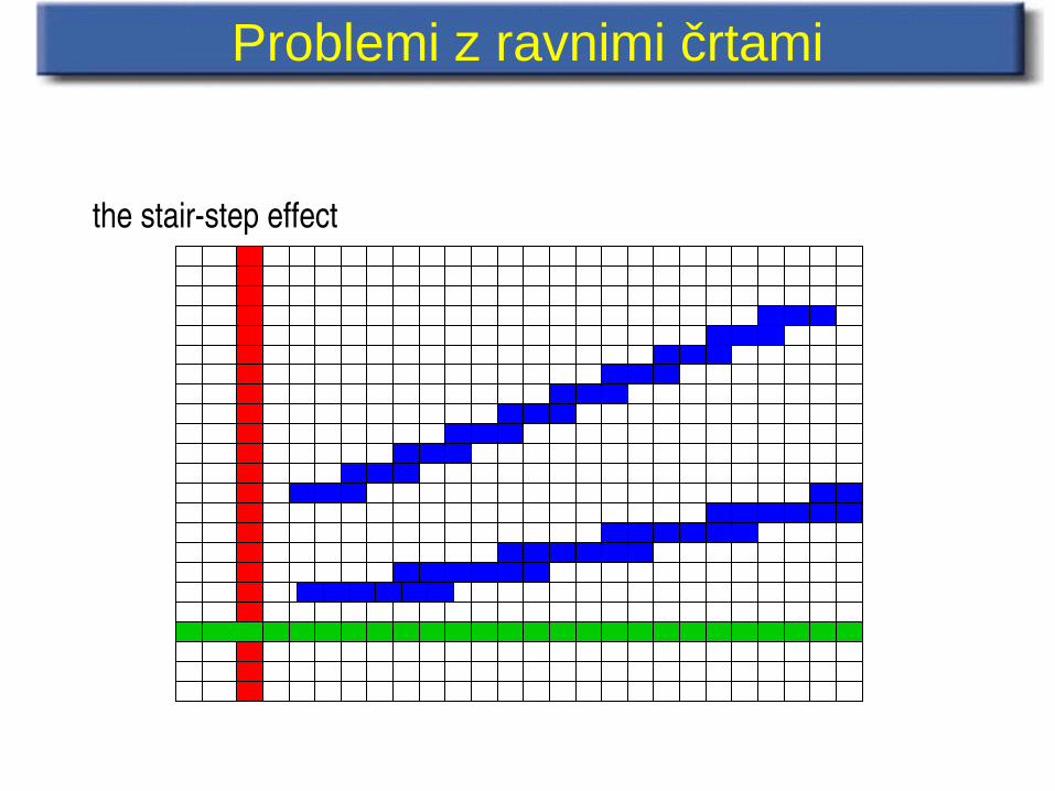
Problemi z ravnimi črtami
the stairstep effect
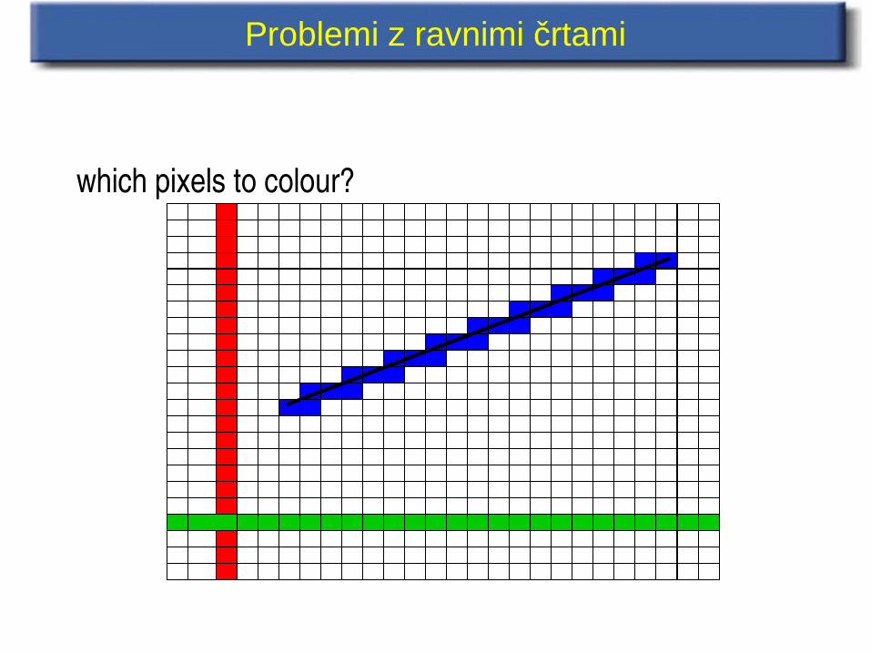
Problemi z ravnimi črtami
which pixels to colour?
Približno risanje črt
• Assume square pixels.• Assume that the line starts at (x1, y1) and
finishes at (x2, y2).• Say that dx=x2-x1, dy=y2-y1• If we start with the simplest non-trivial case
where dx=dy, we can immediately see that a 45 degree diagonal line has one x step per y step.
Približno risanje črt
• The basic requirement for an approximation is to generate the minimum error at each step.
• The largest acceptable error must be half a pixel.
• To simplify the problem, we consider only one eighth of the possible angles, ie we choose to consider only one octant. We can generalise later using a mirroring technique.
Približno risanje črt
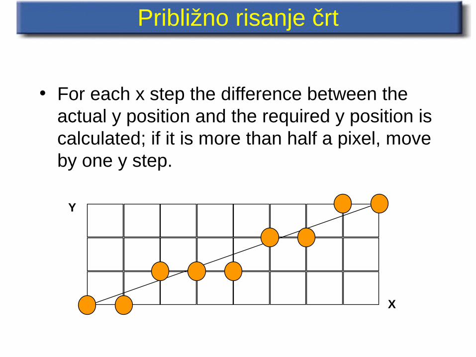
• For each x step the difference between the actual y position and the required y position is calculated; if it is more than half a pixel, move by one y step.
X
Y
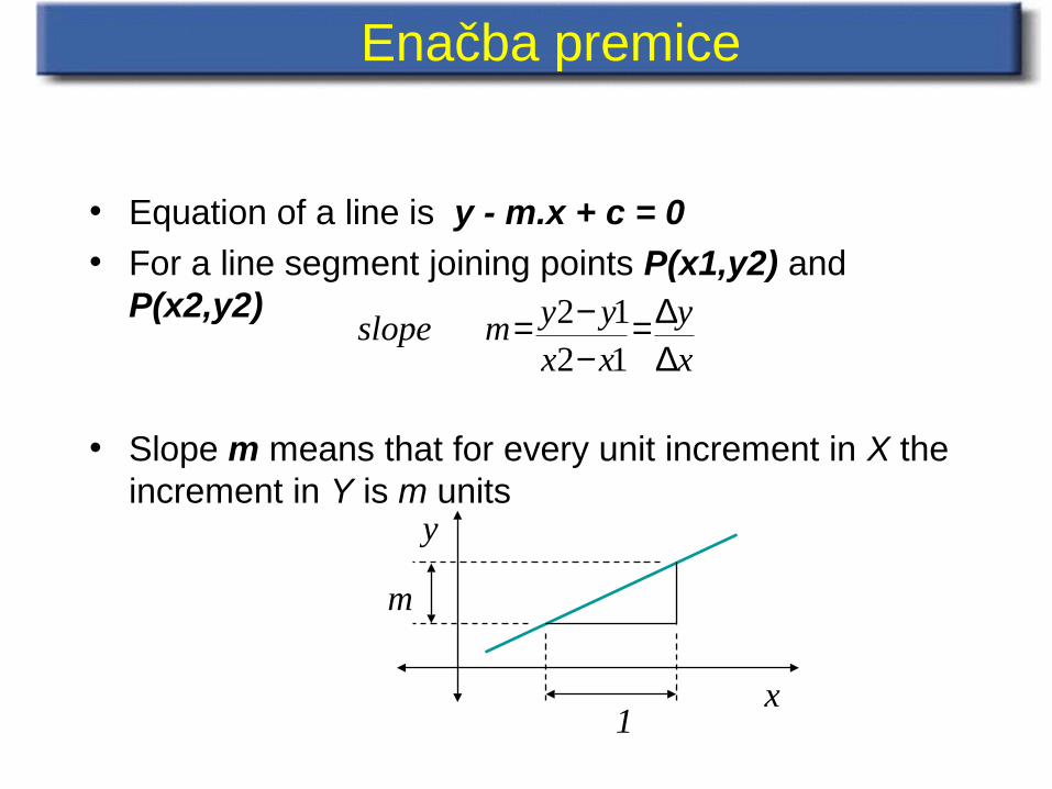
• Equation of a line is y - m.x + c = 0• For a line segment joining points P(x1,y2) and
P(x2,y2)
• Slope m means that for every unit increment in X the increment in Y is m units
Enačba premice
xy
xxyymslope
∆∆=
−−=
1212
1
m
x
y
Naivni algoritem rasterizacije črt
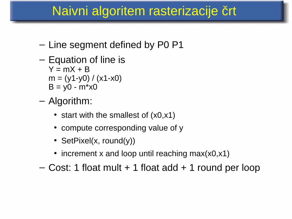
– Line segment defined by P0 P1
– Equation of line isY = mX + Bm = (y1-y0) / (x1-x0)B = y0 - m*x0
– Algorithm: • start with the smallest of (x0,x1)
• compute corresponding value of y
• SetPixel(x, round(y))
• increment x and loop until reaching max(x0,x1)
– Cost: 1 float mult + 1 float add + 1 round per loop
Inkrementalni algoritem rasterizacije črt
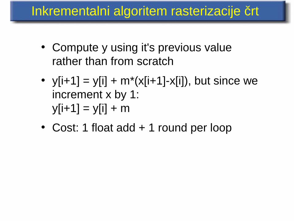
• Compute y using it's previous value rather than from scratch
• y[i+1] = y[i] + m*(x[i+1]-x[i]), but since we increment x by 1:y[i+1] = y[i] + m
• Cost: 1 float add + 1 round per loop
Minimiziranje računanj s plavajočo vejico
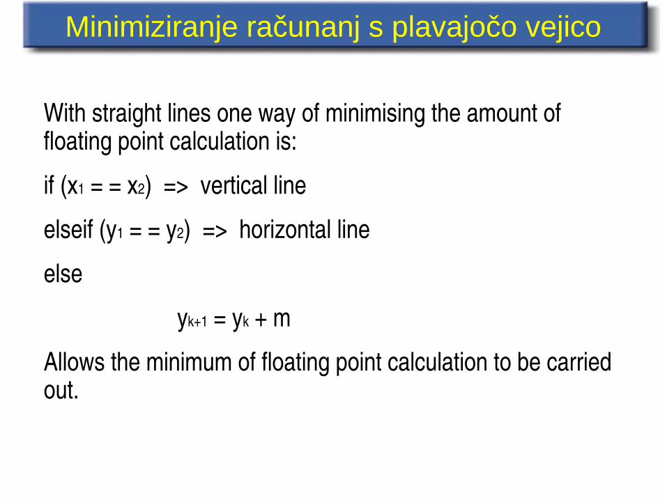
With straight lines one way of minimising the amount of floating point calculation is:
if (x1 = = x2) => vertical line
elseif (y1 = = y2) => horizontal line
else
yk+1 = yk + m
Allows the minimum of floating point calculation to be carried out.
Digitalni diferencialni analizator (DDA)
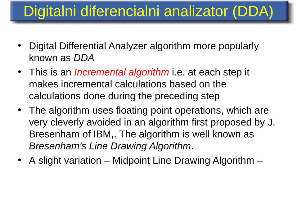
• Digital Differential Analyzer algorithm more popularly known as DDA
• This is an Incremental algorithm i.e. at each step it makes incremental calculations based on the calculations done during the preceding step
• The algorithm uses floating point operations, which are very cleverly avoided in an algorithm first proposed by J. Bresenham of IBM,. The algorithm is well known as Bresenham’s Line Drawing Algorithm.
• A slight variation – Midpoint Line Drawing Algorithm –
Bresenham’s Line Algorithm (BLA)
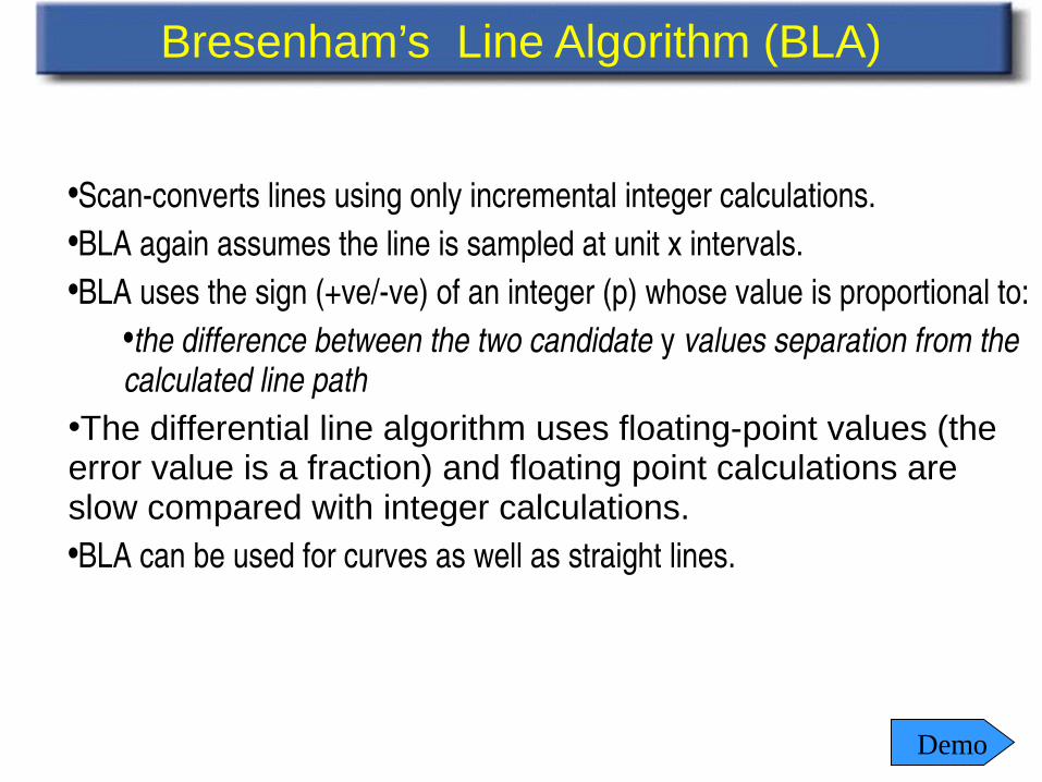
•Scanconverts lines using only incremental integer calculations.•BLA again assumes the line is sampled at unit x intervals.•BLA uses the sign (+ve/ve) of an integer (p) whose value is proportional to:
•the difference between the two candidate y values separation from the calculated line path
•The differential line algorithm uses floating-point values (the error value is a fraction) and floating point calculations are slow compared with integer calculations.•BLA can be used for curves as well as straight lines.
Demo
Digitalni diferencialni analizator (DDA)
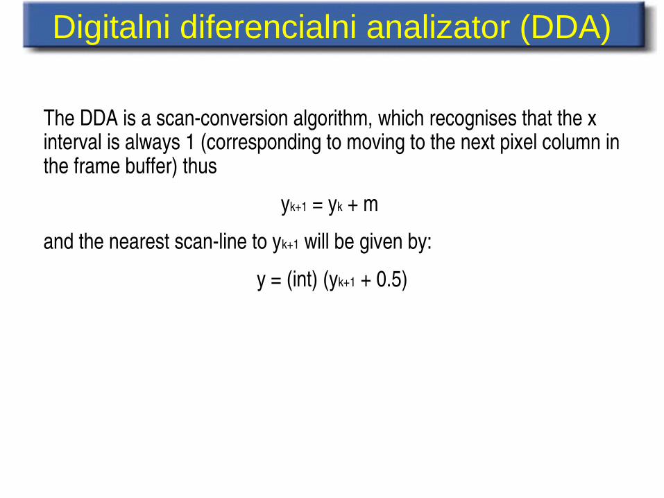
The DDA is a scanconversion algorithm, which recognises that the x interval is always 1 (corresponding to moving to the next pixel column in the frame buffer) thus
yk+1 = yk + m
and the nearest scanline to yk+1 will be given by:
y = (int) (yk+1 + 0.5)
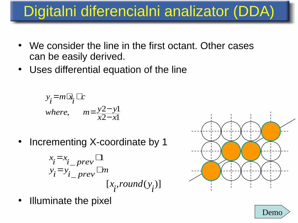
• We consider the line in the first octant. Other cases can be easily derived.
• Uses differential equation of the line
• Incrementing X-coordinate by 1
• Illuminate the pixel
Digitalni diferencialni analizator (DDA)
mpreviyiyprevixix
+=+=
_
1_
1212,
xxyymwhere
cixmiy
−−=
+⋅=
)](,[ iyroundix
Demo
Algoritem DDA
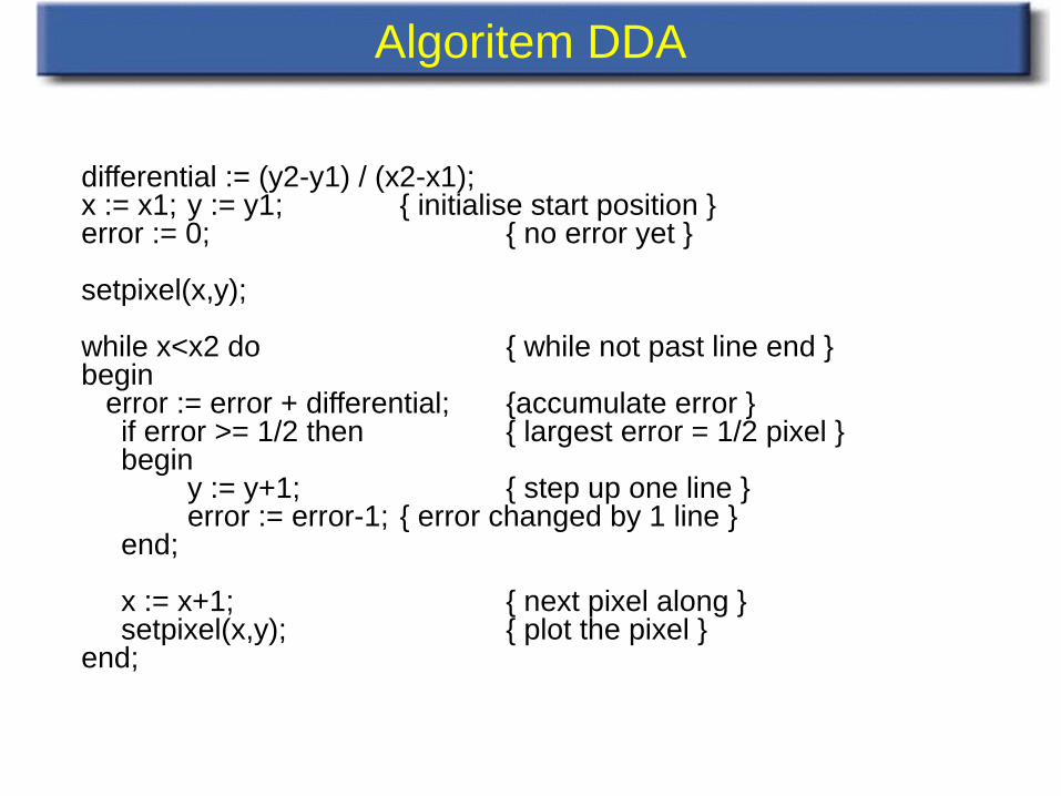
differential := (y2-y1) / (x2-x1);x := x1; y := y1; { initialise start position }error := 0; { no error yet }
setpixel(x,y);
while x<x2 do { while not past line end }begin error := error + differential; {accumulate error } if error >= 1/2 then { largest error = 1/2 pixel } begin y := y+1; { step up one line } error := error-1; { error changed by 1 line } end;
x := x+1; { next pixel along }setpixel(x,y); { plot the pixel }
end;
Značilnosti algoritma DDA
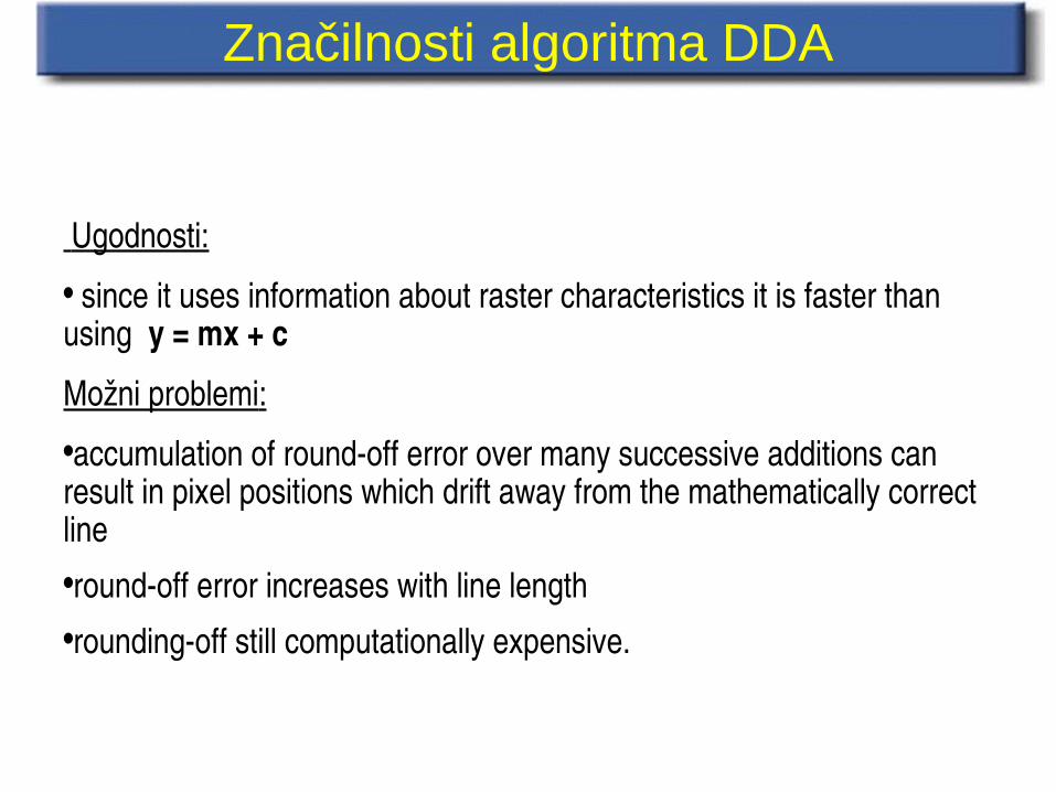
Ugodnosti:
• since it uses information about raster characteristics it is faster than using y = mx + c
Možni problemi:
•accumulation of roundoff error over many successive additions can result in pixel positions which drift away from the mathematically correct line•roundoff error increases with line length•roundingoff still computationally expensive.
Bresenham’s Algorithm: Midpoint Algorithm
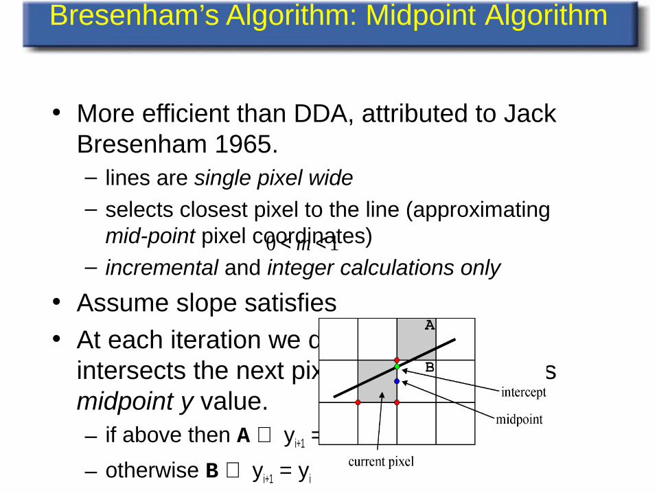
• More efficient than DDA, attributed to Jack Bresenham 1965.– lines are single pixel wide
– selects closest pixel to the line (approximating mid-point pixel coordinates)
– incremental and integer calculations only
• Assume slope satisfies • At each iteration we determine if the line
intersects the next pixel above or below its midpoint y value.– if above then A ⇒ yi+1 = yi+1
– otherwise B ⇒ yi+1 = yi
10 << m
Midpoint Line Algorithm
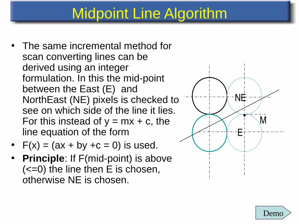
• The same incremental method for scan converting lines can be derived using an integer formulation. In this the mid-point between the East (E) and NorthEast (NE) pixels is checked to see on which side of the line it lies. For this instead of y = mx + c, the line equation of the form
• F(x) = (ax + by +c = 0) is used. • Principle: If F(mid-point) is above
(<=0) the line then E is chosen, otherwise NE is chosen.
NE
E
• M
Demo
Midpoint Line Algorithm
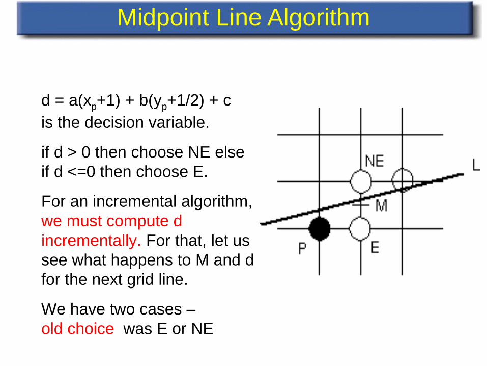
d = a(xp+1) + b(yp+1/2) + c is the decision variable.
if d > 0 then choose NE else if d <=0 then choose E.
For an incremental algorithm, we must compute d incrementally. For that, let us see what happens to M and d for the next grid line.
We have two cases – old choice was E or NE
Midpoint Line Algorithm (nadaljevanje)
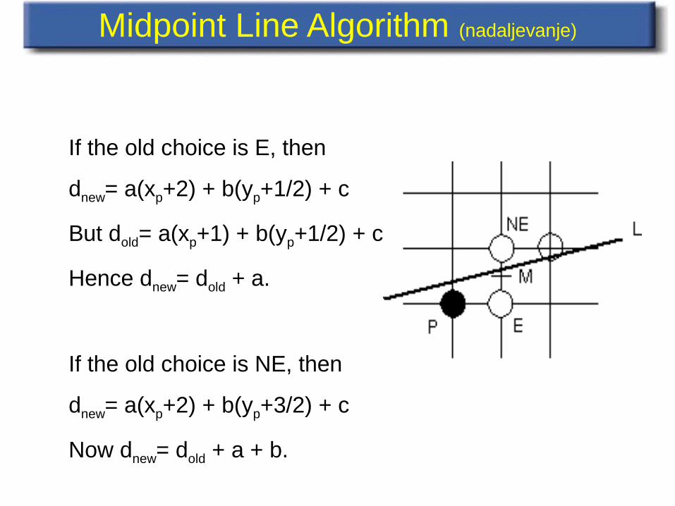
If the old choice is E, then
dnew= a(xp+2) + b(yp+1/2) + c
But dold= a(xp+1) + b(yp+1/2) + c
Hence dnew= dold + a.
If the old choice is NE, then
dnew= a(xp+2) + b(yp+3/2) + c
Now dnew= dold + a + b.
Midpoint Line Algorithm (nadaljevanje)
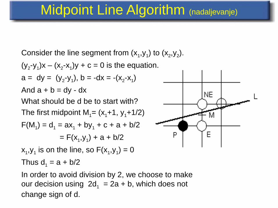
Consider the line segment from (x1,y1) to (x2,y2).
(y2-y1)x – (x2-x1)y + c = 0 is the equation.
a = dy = (y2-y1), b = -dx = -(x2-x1)
And a + b = dy - dx
What should be d be to start with?
The first midpoint M1= (x1+1, y1+1/2)
F(M1) = d1 = ax1 + by1 + c + a + b/2
= F(x1,y1) + a + b/2
x1,y1 is on the line, so F(x1,y1) = 0
Thus d1 = a + b/2
In order to avoid division by 2, we choose to make our decision using 2d1 = 2a + b, which does not change sign of d.
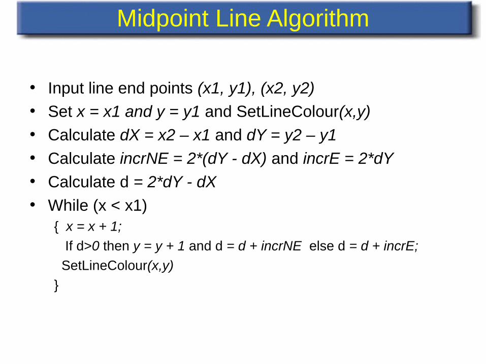
• Input line end points (x1, y1), (x2, y2)• Set x = x1 and y = y1 and SetLineColour(x,y)
• Calculate dX = x2 – x1 and dY = y2 – y1
• Calculate incrNE = 2*(dY - dX) and incrE = 2*dY• Calculate d = 2*dY - dX• While (x < x1)
{ x = x + 1;
If d>0 then y = y + 1 and d = d + incrNE else d = d + incrE;
SetLineColour(x,y)
}
Midpoint Line Algorithm
Midpoint Line Algorithm
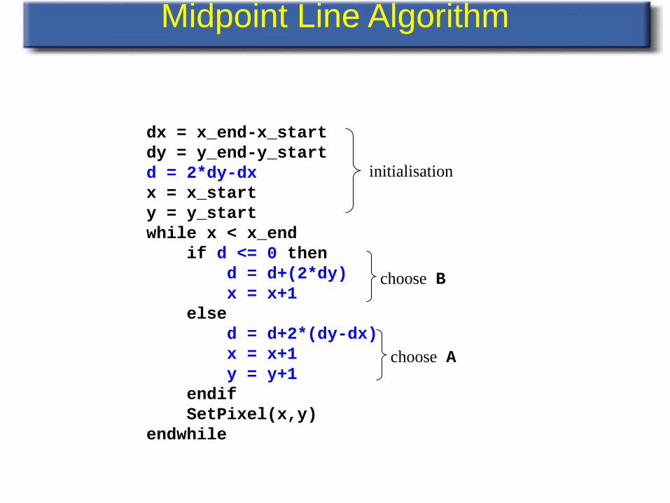
dx = x_end-x_startdy = y_end-y_startd = 2*dy-dxx = x_starty = y_startwhile x < x_end if d <= 0 then d = d+(2*dy) x = x+1 else d = d+2*(dy-dx) x = x+1 y = y+1 endif SetPixel(x,y)endwhile
initialisation
choose B
choose A
Midpoint Line Algorithm
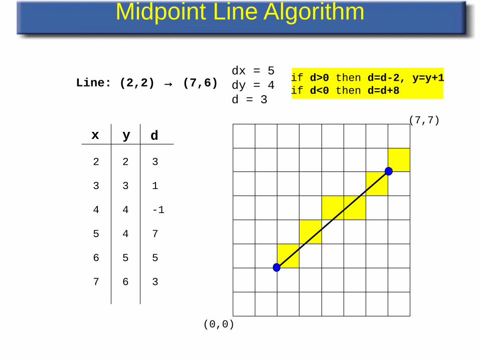
(0,0)
(7,7)
Line: (2,2) → (7,6)dx = 5dy = 4d = 3
x y
3 3 1
4 4 -1
5 4 7
6 5 5
7 6 3
2 2 3
d
if d>0 then d=d-2, y=y+1if d<0 then d=d+8
Advantages of Incremental Midpoint Line Algorithm
• It is an incremental algorithm• It uses only integer arithmetic• Provides the best fit approximation to the actual
line

Algoritmi za kroge
• Circle with radius r and center (xc, yc) is defined parametrically as:
∴ could step through θ from 0 to 2π plotting co-ordinates:– difficult to effectively control step-size to eliminate gaps and
minimise pixel overdrawing
θθ
sin
cos
ryy
rxx
c
c
+=+=
Bresenham’s Circle Algorithm
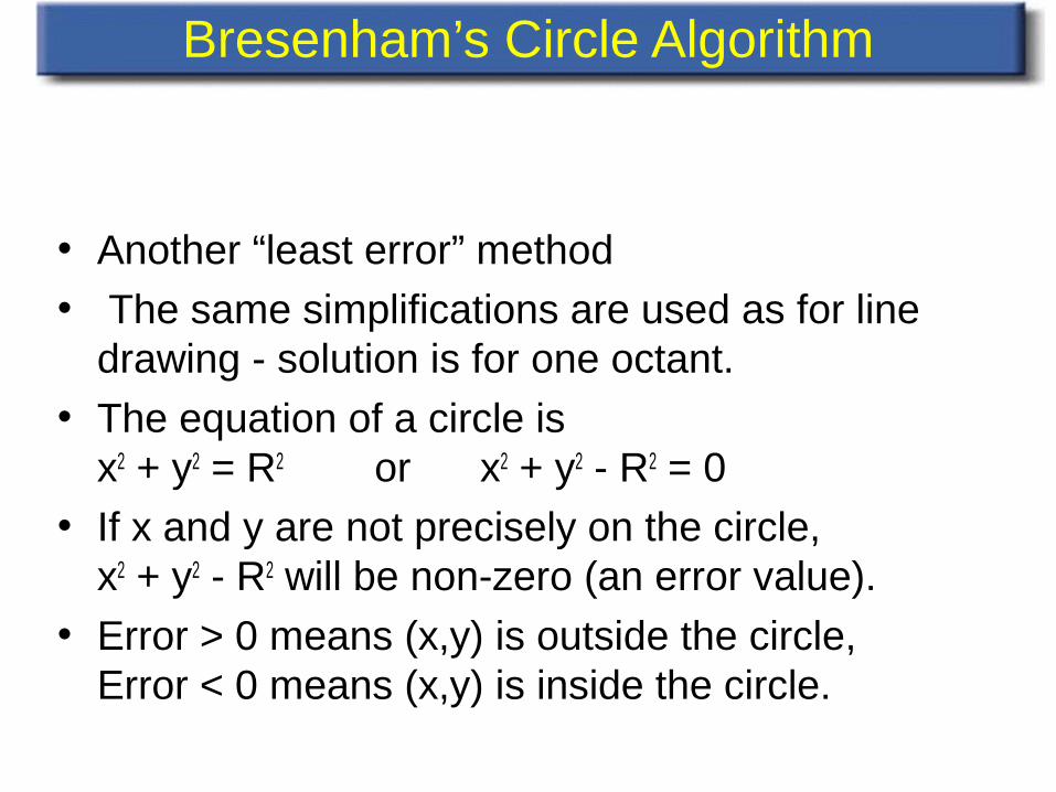
• Another “least error” method• The same simplifications are used as for line
drawing - solution is for one octant.• The equation of a circle is
x2 + y2 = R2 or x2 + y2 - R2 = 0• If x and y are not precisely on the circle,
x2 + y2 - R2 will be non-zero (an error value).• Error > 0 means (x,y) is outside the circle,
Error < 0 means (x,y) is inside the circle.
Midpoint Circle Algorithm
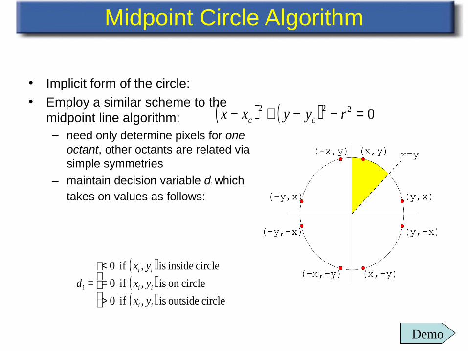
• Implicit form of the circle:• Employ a similar scheme to the
midpoint line algorithm:– need only determine pixels for one
octant, other octants are related via simple symmetries
– maintain decision variable di which takes on values as follows:
( ) ( ) 0222 =−−+− ryyxx cc
( )( )( )
circle outside is , if 0
circleon is , if 0
circle inside is , if 0
>=<
=
ii
ii
ii
i
yx
yx
yx
d
Demo
Midpoint Circle Algorithm
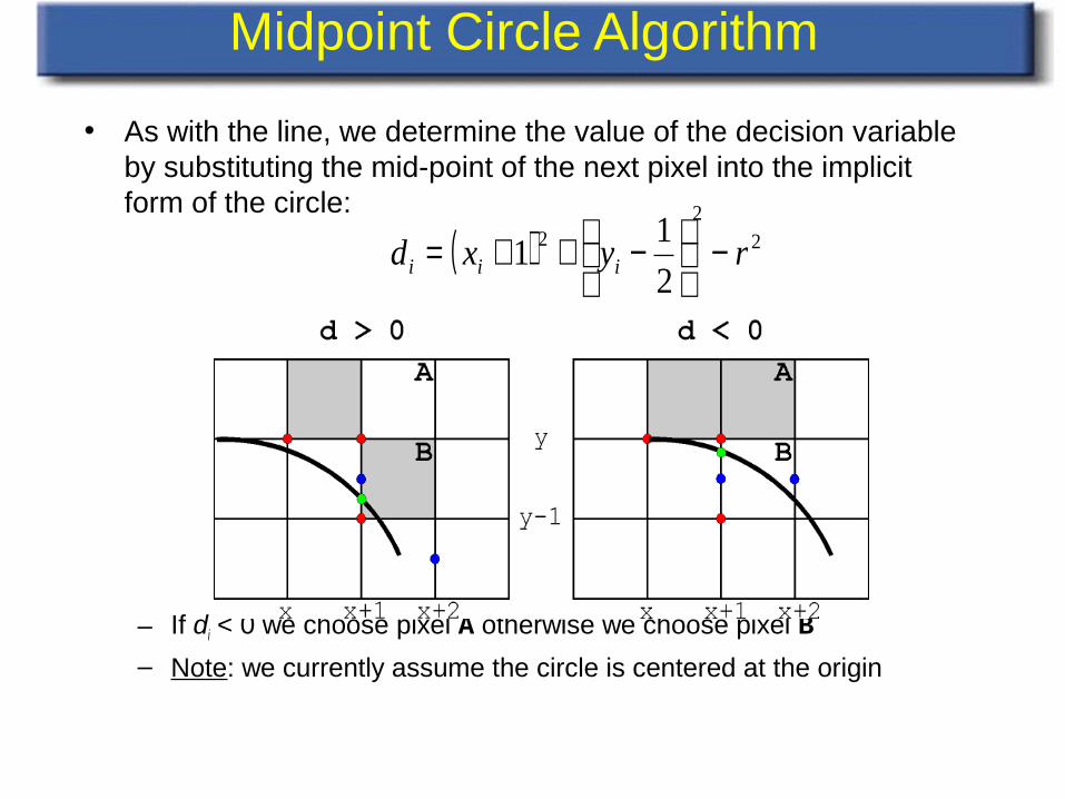
• As with the line, we determine the value of the decision variable by substituting the mid-point of the next pixel into the implicit form of the circle:
– If di < 0 we choose pixel A otherwise we choose pixel B
– Note: we currently assume the circle is centered at the origin
( ) 22
2
2
11 ryxd iii −
−++=
Midpoint Circle Algorithm
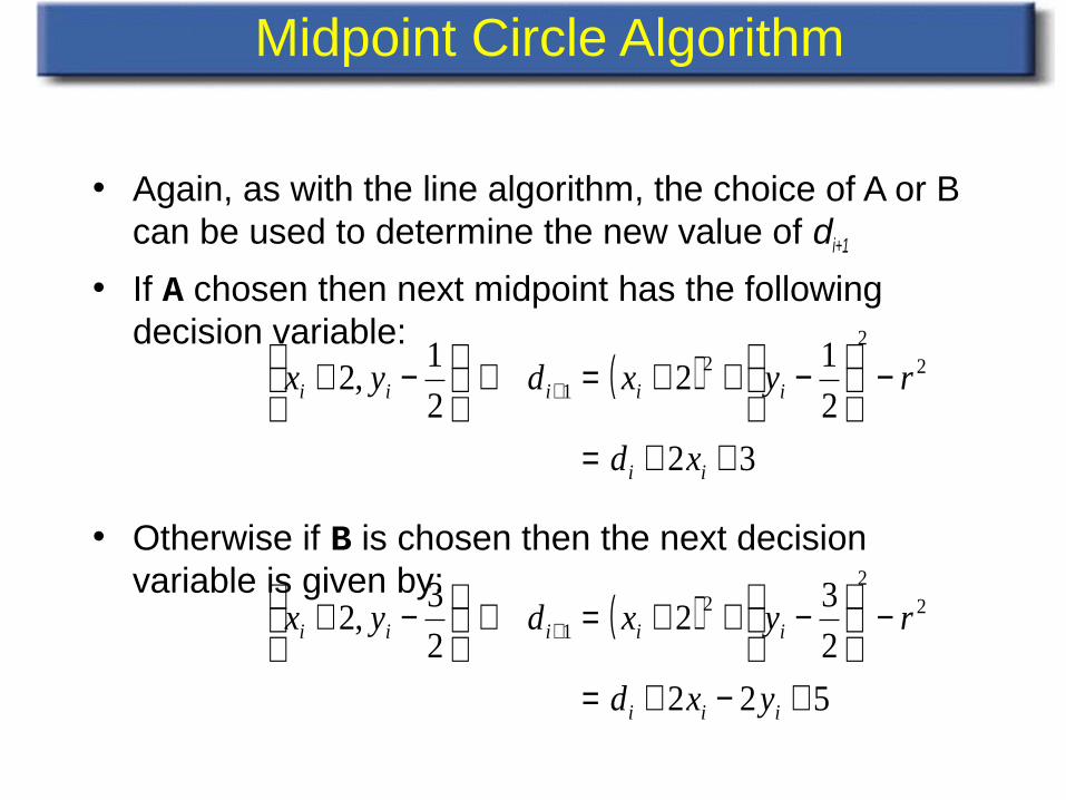
• Again, as with the line algorithm, the choice of A or B can be used to determine the new value of di+1
• If A chosen then next midpoint has the following decision variable:
• Otherwise if B is chosen then the next decision variable is given by:
( )
32
2
12
2
1,2 2
22
1
++=
−
−++=⇒
−+ +
ii
iiiii
xd
ryxdyx
( )
522
2
32
2
3,2 2
22
1
+−+=
−
−++=⇒
−+ +
iii
iiiii
yxd
ryxdyx
Midpoint Circle Algorithm
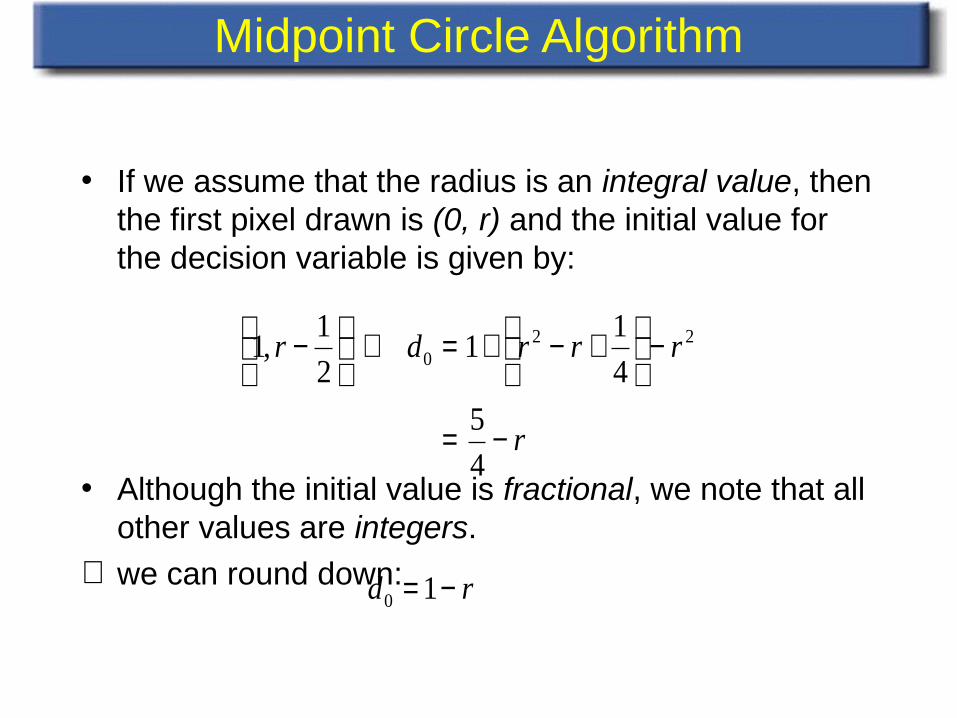
• If we assume that the radius is an integral value, then the first pixel drawn is (0, r) and the initial value for the decision variable is given by:
• Although the initial value is fractional, we note that all other values are integers.
⇒ we can round down:
r
rrrdr
−=
−
+−+=⇒
−
4
5
4
11
2
1,1 22
0
rd −= 10
Midpoint Circle Algorithm
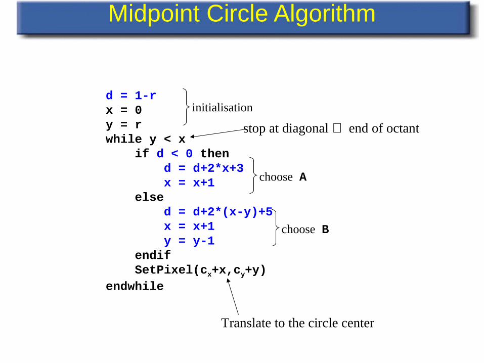
d = 1-rx = 0y = rwhile y < x if d < 0 then d = d+2*x+3 x = x+1 else d = d+2*(x-y)+5 x = x+1 y = y-1 endif SetPixel(cx+x,cy+y)endwhile
initialisation
choose B
choose A
Translate to the circle center
stop at diagonal ⇒ end of octant
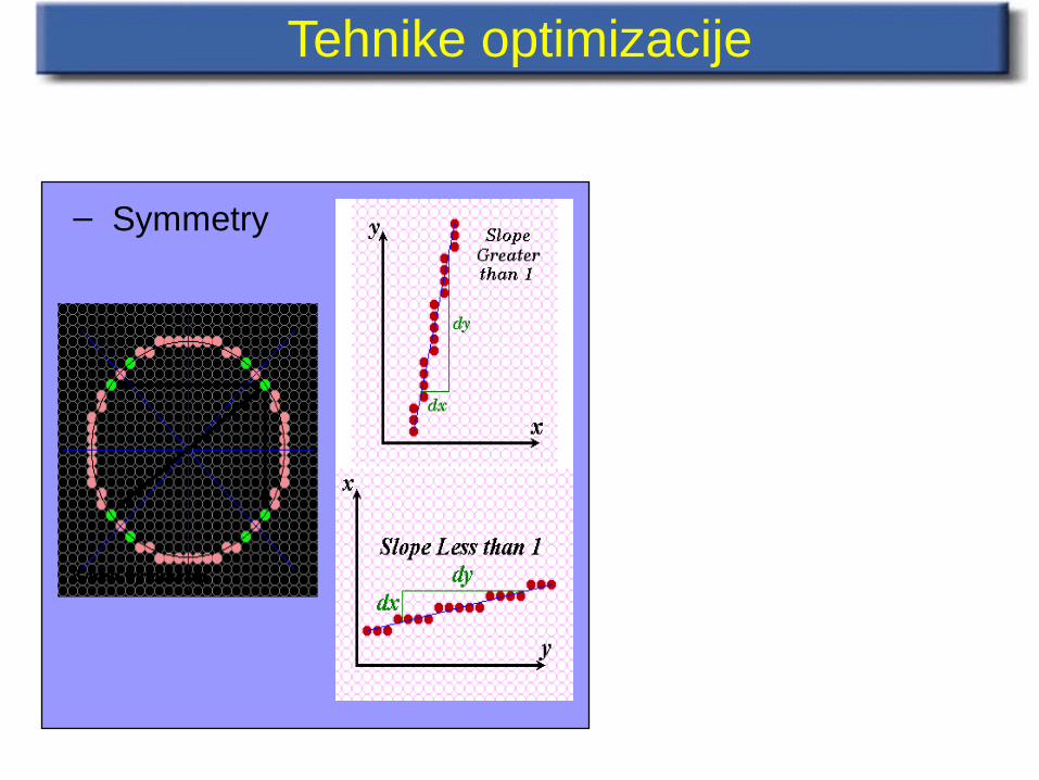
Tehnike optimizacije
– Symmetry
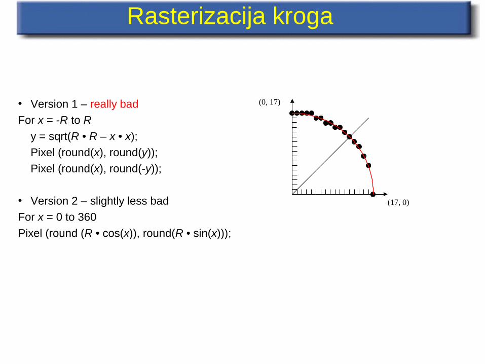
• Version 1 – really bad
For x = -R to R
y = sqrt(R • R – x • x);
Pixel (round(x), round(y));
Pixel (round(x), round(-y));
• Version 2 – slightly less bad
For x = 0 to 360
Pixel (round (R • cos(x)), round(R • sin(x)));
(17, 0)
(0, 17)
Rasterizacija kroga
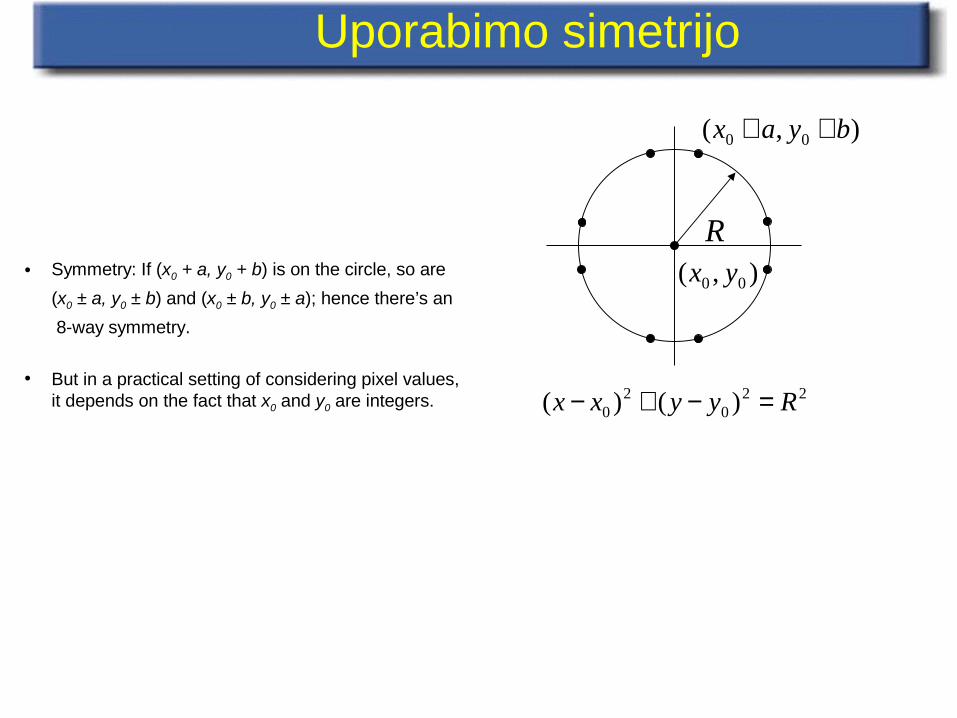
• Symmetry: If (x0 + a, y0 + b) is on the circle, so are
(x0 ± a, y0 ± b) and (x0 ± b, y0 ± a); hence there’s an
8-way symmetry.
• But in a practical setting of considering pixel values, it depends on the fact that x0 and y0 are integers.
Uporabimo simetrijo
220
20 )()( Ryyxx =−+−
R),( 00 yx
),( 00 byax ++
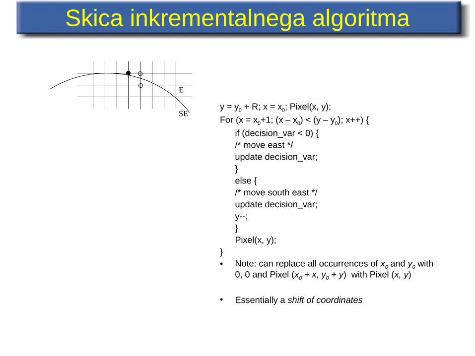
y = y0 + R; x = x0; Pixel(x, y);
For (x = x0+1; (x – x0) < (y – y0); x++) {
if (decision_var < 0) {/* move east */update decision_var;}else {/* move south east */update decision_var;y--;}Pixel(x, y);
}• Note: can replace all occurrences of x0 and y0 with
0, 0 and Pixel (x0 + x, y0 + y) with Pixel (x, y)
• Essentially a shift of coordinates
Skica inkrementalnega algoritma
E
SE
Poligoni
Poligoni
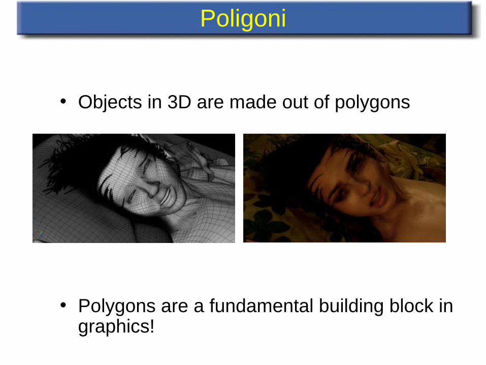
• Objects in 3D are made out of polygons
• Polygons are a fundamental building block in graphics!
Rasterizacija poligonov
• In interactive graphics, polygons rule the world• Two main reasons:
– Lowest common denominator for surfaces• Can represent any surface with arbitrary accuracy• Splines, mathematical functions, volumetric isosurfaces…
– Mathematical simplicity lends itself to simple, regular rendering algorithms
• Like those we’re about to discuss… • Such algorithms embed well in hardware
Rasterizacija poligonov
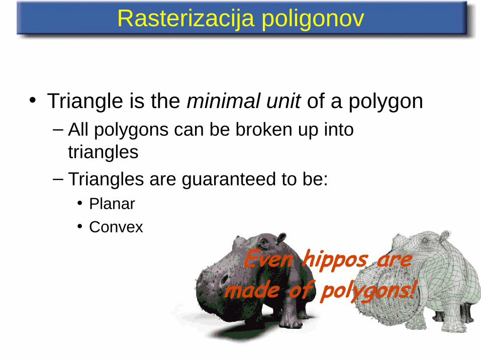
• Triangle is the minimal unit of a polygon– All polygons can be broken up into
triangles– Triangles are guaranteed to be:
• Planar
• Convex
Rasterizacija poligonov
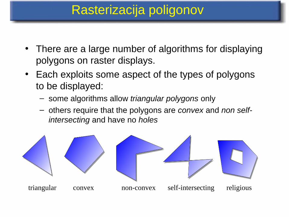
• There are a large number of algorithms for displaying polygons on raster displays.
• Each exploits some aspect of the types of polygons to be displayed:– some algorithms allow triangular polygons only– others require that the polygons are convex and non self-
intersecting and have no holes
triangular convex non-convex self-intersecting religious
Rasterizacija poligonov
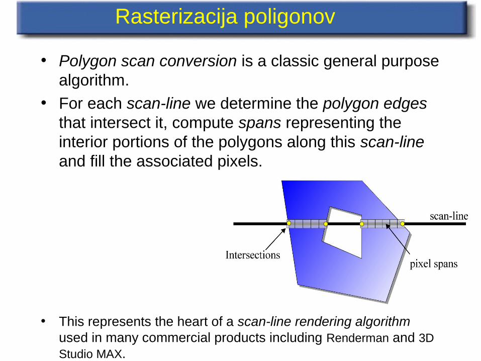
• Polygon scan conversion is a classic general purpose algorithm.
• For each scan-line we determine the polygon edges that intersect it, compute spans representing the interior portions of the polygons along this scan-line and fill the associated pixels.
• This represents the heart of a scan-line rendering algorithm used in many commercial products including Renderman and 3D Studio MAX.
Rasterizacija poligonov
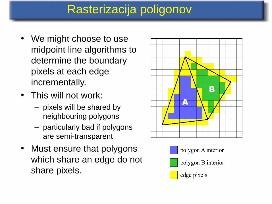
• We might choose to use midpoint line algorithms to determine the boundary pixels at each edge incrementally.
• This will not work:– pixels will be shared by
neighbouring polygons– particularly bad if polygons
are semi-transparent
• Must ensure that polygons which share an edge do not share pixels.
Rasterizacija poligonov
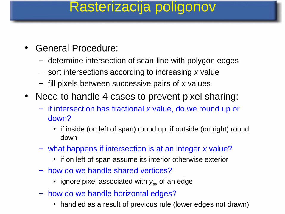
• General Procedure:– determine intersection of scan-line with polygon edges– sort intersections according to increasing x value– fill pixels between successive pairs of x values
• Need to handle 4 cases to prevent pixel sharing:– if intersection has fractional x value, do we round up or
down?• if inside (on left of span) round up, if outside (on right) round
down
– what happens if intersection is at an integer x value?• if on left of span assume its interior otherwise exterior
– how do we handle shared vertices?• ignore pixel associated with ymax of an edge
– how do we handle horizontal edges?• handled as a result of previous rule (lower edges not drawn)
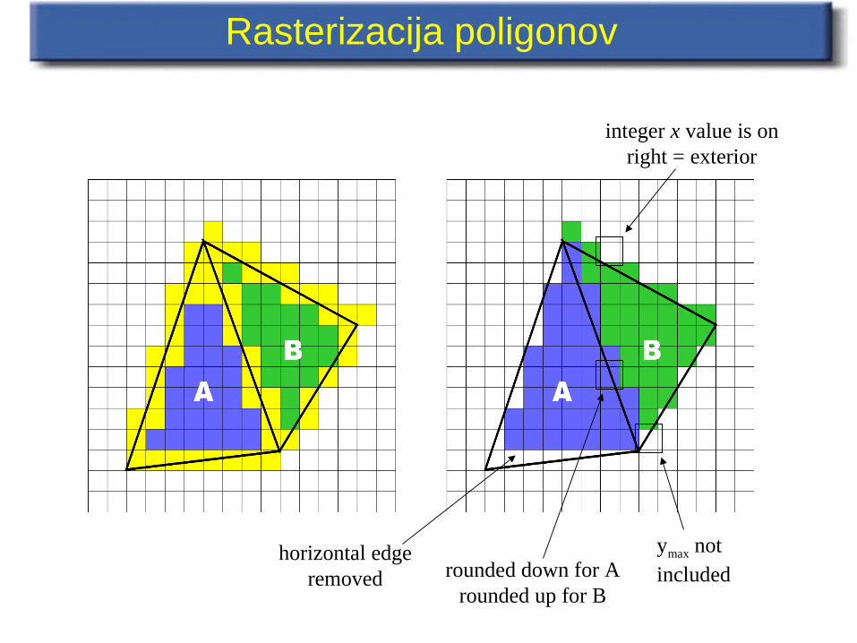
Rasterizacija poligonov
rounded down for Arounded up for B
integer x value is onright = exterior
ymax not included
horizontal edgeremoved
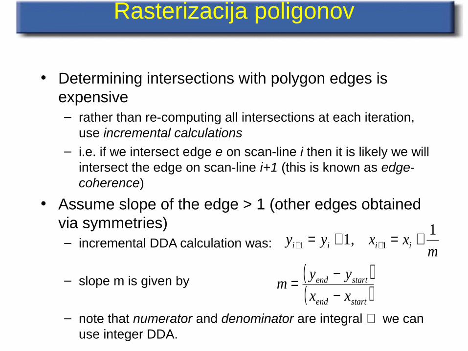
Rasterizacija poligonov
• Determining intersections with polygon edges is expensive– rather than re-computing all intersections at each iteration,
use incremental calculations– i.e. if we intersect edge e on scan-line i then it is likely we will
intersect the edge on scan-line i+1 (this is known as edge-coherence)
• Assume slope of the edge > 1 (other edges obtained via symmetries)– incremental DDA calculation was:
– slope m is given by
– note that numerator and denominator are integral ⇒ we can use integer DDA.
mxxyy iiii
1,1 11 +=+= ++
( )( )startend
startend
xx
yym
−−=
Metode rasterizacije
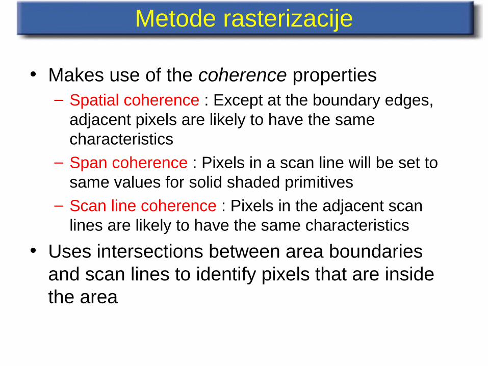
• Makes use of the coherence properties – Spatial coherence : Except at the boundary edges,
adjacent pixels are likely to have the same characteristics
– Span coherence : Pixels in a scan line will be set to same values for solid shaded primitives
– Scan line coherence : Pixels in the adjacent scan lines are likely to have the same characteristics
• Uses intersections between area boundaries and scan lines to identify pixels that are inside the area
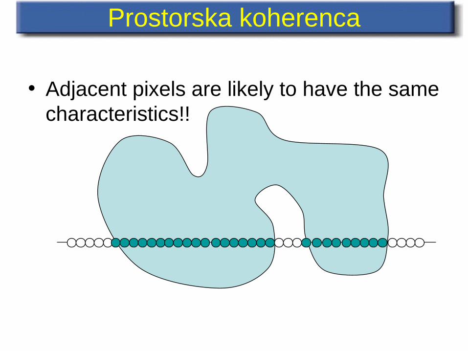
• Adjacent pixels are likely to have the same characteristics!!
Prostorska koherenca
Rasterizacija poligonov
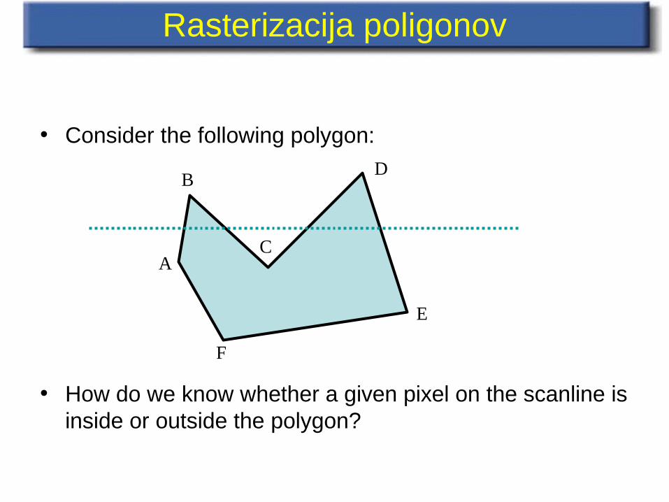
• Consider the following polygon:
• How do we know whether a given pixel on the scanline is inside or outside the polygon?
A
B
C
D
E
F
Rasterizacija poligonov
A B
D C
F
EH G
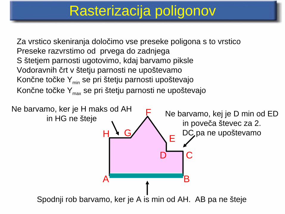
Za vrstico skeniranja določimo vse preseke poligona s to vrsticoPreseke razvrstimo od prvega do zadnjegaS štetjem parnosti ugotovimo, kdaj barvamo piksleVodoravnih črt v štetju parnosti ne upoštevamoKončne točke Ymin se pri štetju parnosti upoštevajoKončne točke Ymax se pri štetju parnosti ne upoštevajo
Spodnji rob barvamo, ker je A is min od AH. AB pa ne šteje
Ne barvamo, ker je H maks od AHin HG ne šteje
Ne barvamo, kej je D min od EDin poveča števec za 2.DC pa ne upoštevamo
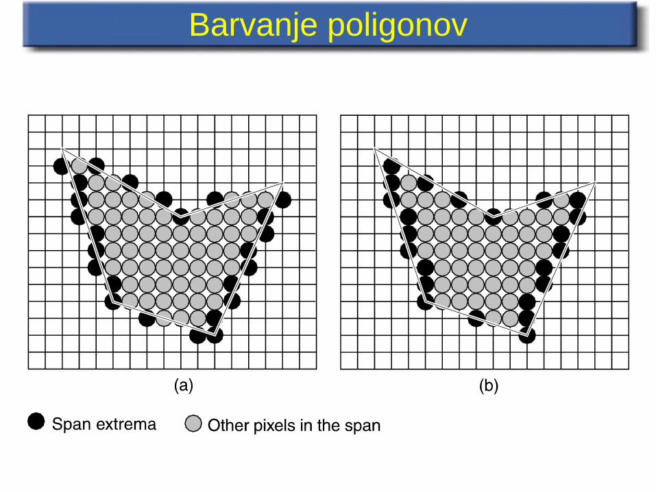
Barvanje poligonov
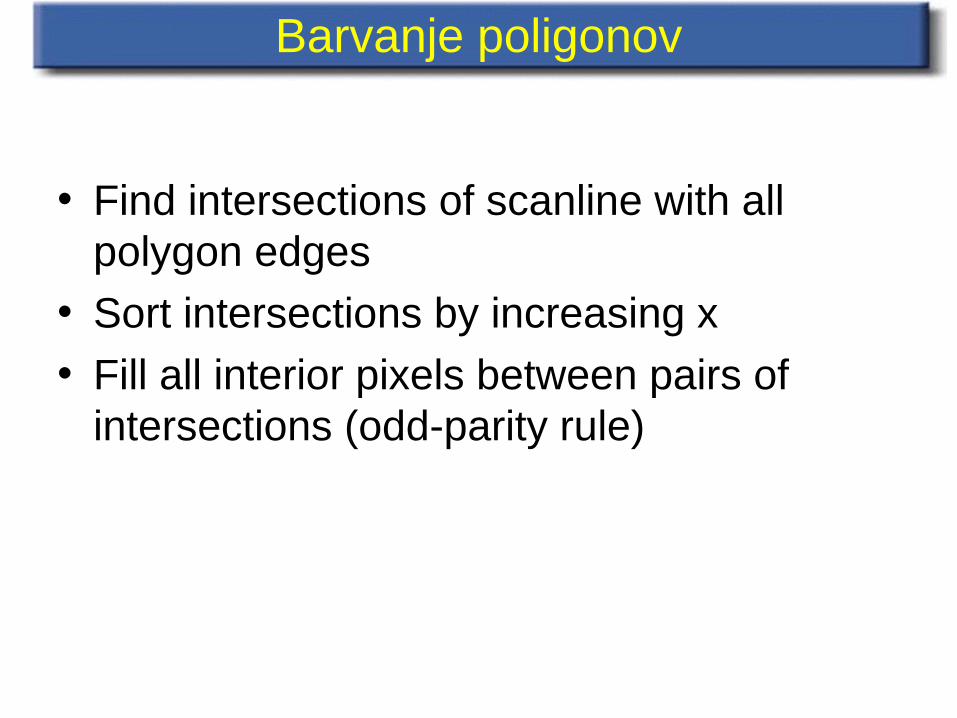
• Find intersections of scanline with all polygon edges
• Sort intersections by increasing x
• Fill all interior pixels between pairs of intersections (odd-parity rule)
Barvanje poligonov
Prednosti metode Scan Line
• The algorithm is efficient• Each pixel is visited only once• Shading algorithms could be easily integrated
with this method to obtain shaded area
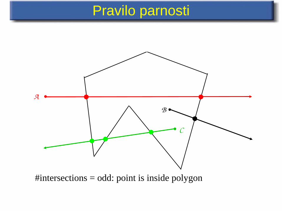
Pravilo parnosti
A
B
C
#intersections = odd: point is inside polygon
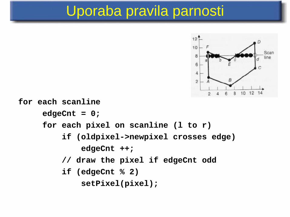
Uporaba pravila parnosti
for each scanline
edgeCnt = 0;
for each pixel on scanline (l to r)
if (oldpixel->newpixel crosses edge)
edgeCnt ++;
// draw the pixel if edgeCnt odd
if (edgeCnt % 2)
setPixel(pixel);
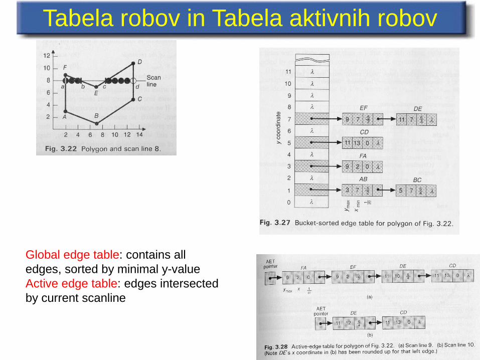
Tabela robov in Tabela aktivnih robov
Global edge table: contains all edges, sorted by minimal y-valueActive edge table: edges intersected by current scanline
Tabela robov (ET, Edge Table)
• Polje kazalcev A, dolžina enaka višini zaslona
• A[i] kaže na povezan seznam vseh robov z ymin = I
• Robovi v povezanem seznamu so razvrščeni glede na koordinato x verteksa ymin
• Rob v seznamu je predstavljen z: ymax, začetnim x, naklonom (1/m)
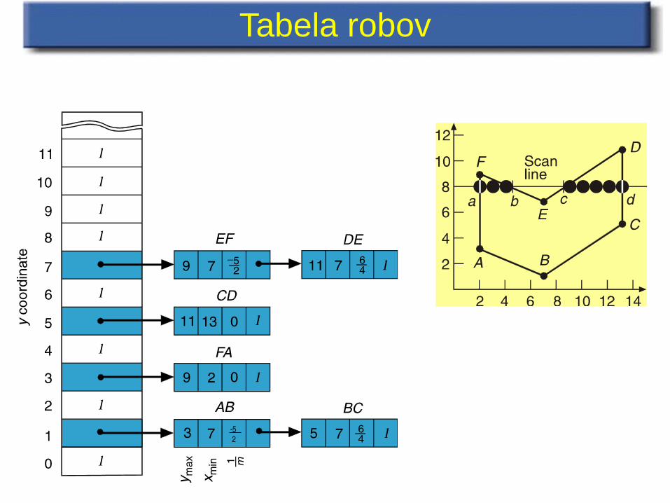
Tabela robov
5 2

Tabela aktivnih robov
Povezan seznam vseh robov, ki sekajo tekočo vrstico skeniranja
Seznam vedno uredimo glede na sekanje x z vrstico skeniranja
Najprej dodamo vse robove iz te tabele z najmanjšim y
S testom parnosti zapolnjujemo (barvamo) piksle na vrstici skeniranja
Vrstico skeniranja premikamo navzgor
Dodajamo vse robove iz tabele robov, pri katerih je vrednost ymin enaka vrstici skeniranja
Odstranimo vse robove iz tabele aktivnih robov, pri katerih je vrednost ymax enaka vrstici skeniranja
Posodobimo vrednosti x vrednosti presečišč vseh robov v aktivni tabeli robov in prerarvrstimo
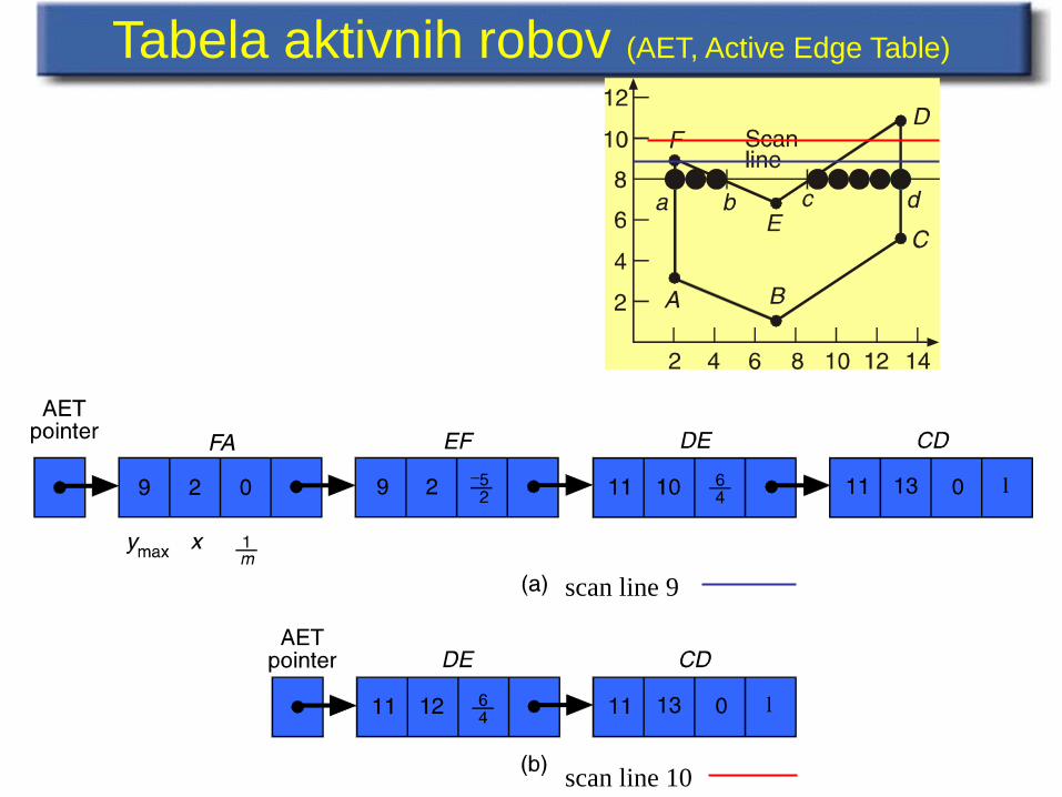
Tabela aktivnih robov (AET, Active Edge Table)
scan line 9
scan line 10
Algoritem
• The scan-line algorithm uses edge-coherence and incremental integer calculations for maximum efficiency:– create an edge table (ET) which lists all edges in order to their
ymin value
– keep track of an active edge table (AET) which lists those edges under the current scan-line
• As the scan progresses, edges are moved from the ET to the AET.
• An edge remains in the AET until ymax for that edge has been reached.
• At this point the edge is removed from the AET.
Algoritem
• Initialize edge table• y = smallest ymin from edge table• active edge table = empty• Repeat:
– Update active edge table: remove, add, sort on x– Fill pixels– Increment y– Update x for each span
• Untill active edge table and edge table empty
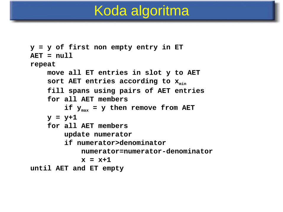
Koda algoritma
y = y of first non empty entry in ETAET = nullrepeat move all ET entries in slot y to AET sort AET entries according to xmin
fill spans using pairs of AET entries for all AET members if ymax = y then remove from AET y = y+1 for all AET members update numerator if numerator>denominator numerator=numerator-denominator x = x+1until AET and ET empty
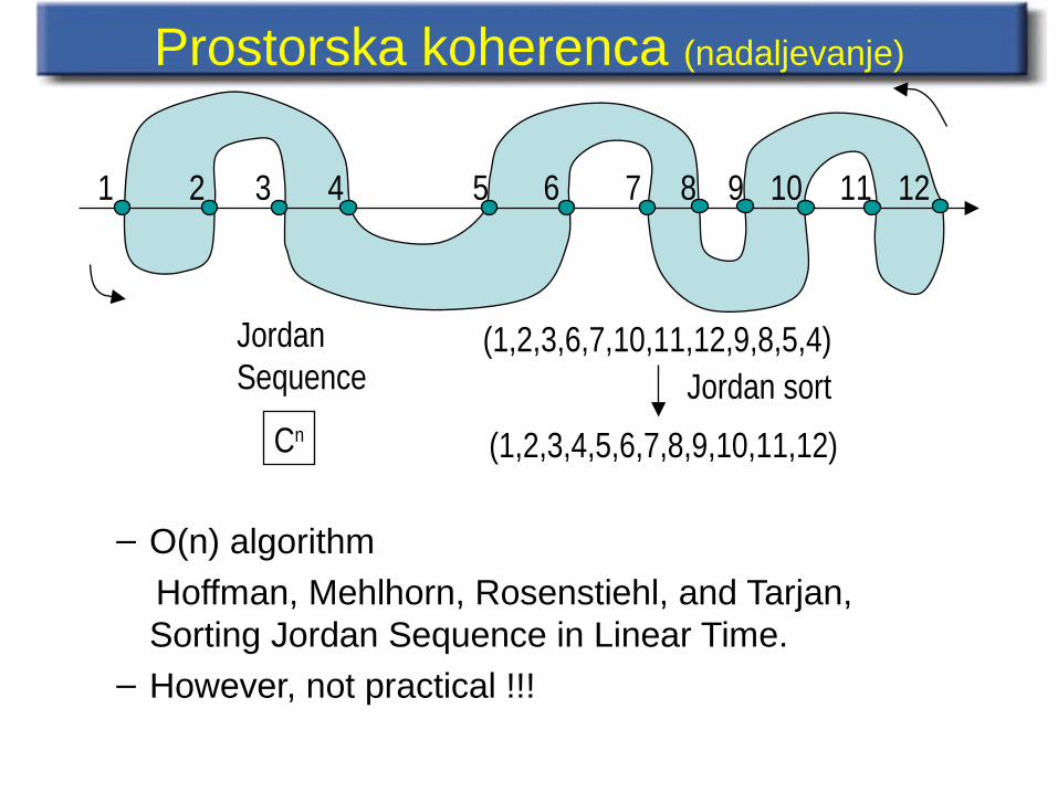
Prostorska koherenca (nadaljevanje)
– O(n) algorithm
Hoffman, Mehlhorn, Rosenstiehl, and Tarjan, Sorting Jordan Sequence in Linear Time.
– However, not practical !!!
1 2 3 4 5 6 7 8 9 10 11 12
JordanSequence
(1,2,3,6,7,10,11,12,9,8,5,4)
(1,2,3,4,5,6,7,8,9,10,11,12)
Jordan sort
Cn
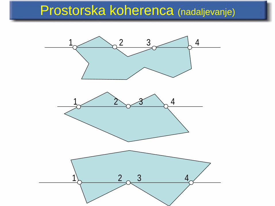
Prostorska koherenca (nadaljevanje)
1 2 3 4
1 2 3 4
1 2 3 4
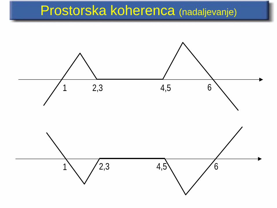
1 2,3 4,5 6
1 2,3 4,5 6
Prostorska koherenca (nadaljevanje)
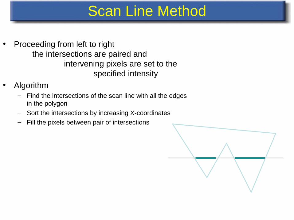
Scan Line Method
• Proceeding from left to right the intersections are paired and
intervening pixels are set to the specified intensity
• Algorithm– Find the intersections of the scan line with all the edges
in the polygon– Sort the intersections by increasing X-coordinates– Fill the pixels between pair of intersections
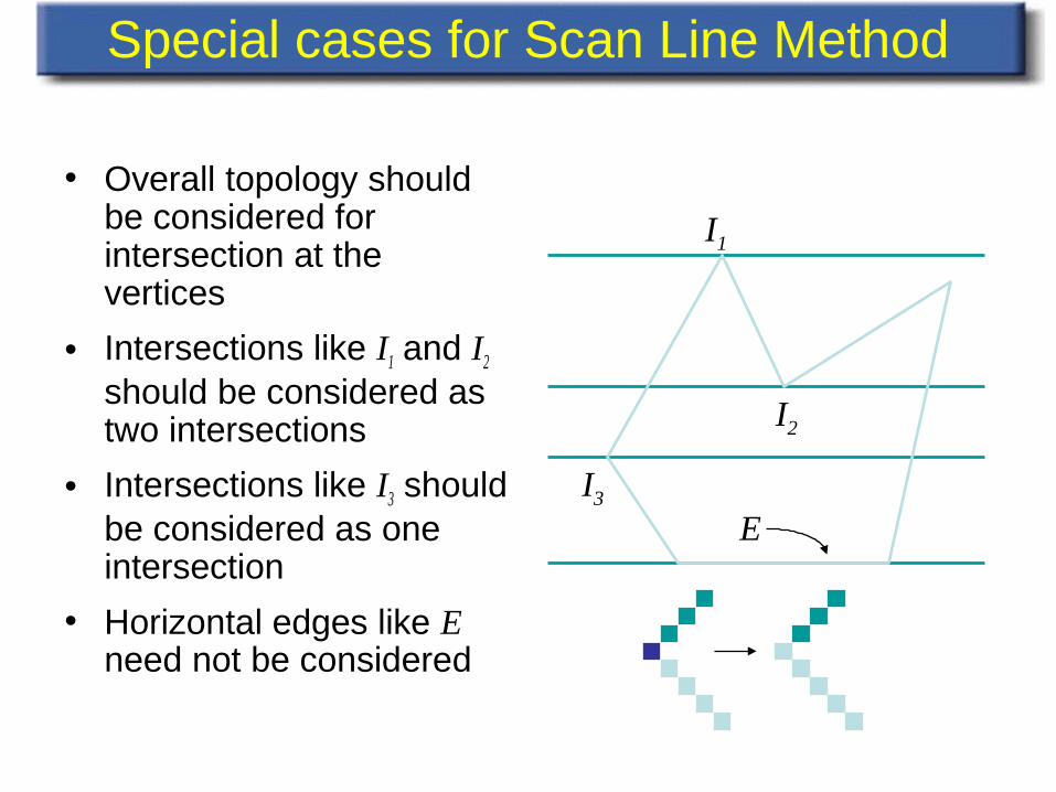
Special cases for Scan Line Method
• Overall topology should be considered for intersection at the vertices
• Intersections like I1 and I2 should be considered as two intersections
• Intersections like I3 should be considered as one intersection
• Horizontal edges like E need not be considered
I1
I2
I3
E
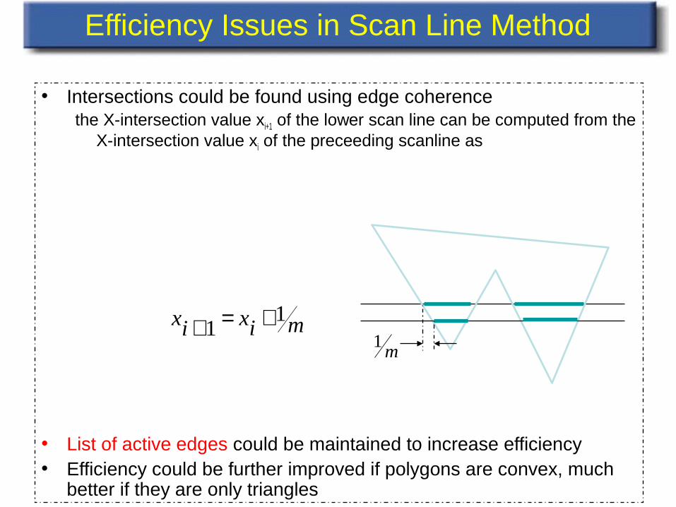
• Intersections could be found using edge coherencethe X-intersection value xi+1 of the lower scan line can be computed from the
X-intersection value xi of the preceeding scanline as
• List of active edges could be maintained to increase efficiency• Efficiency could be further improved if polygons are convex, much
better if they are only triangles
Efficiency Issues in Scan Line Method
xi xi m+ = +11
m1
Bilinear Interpolation
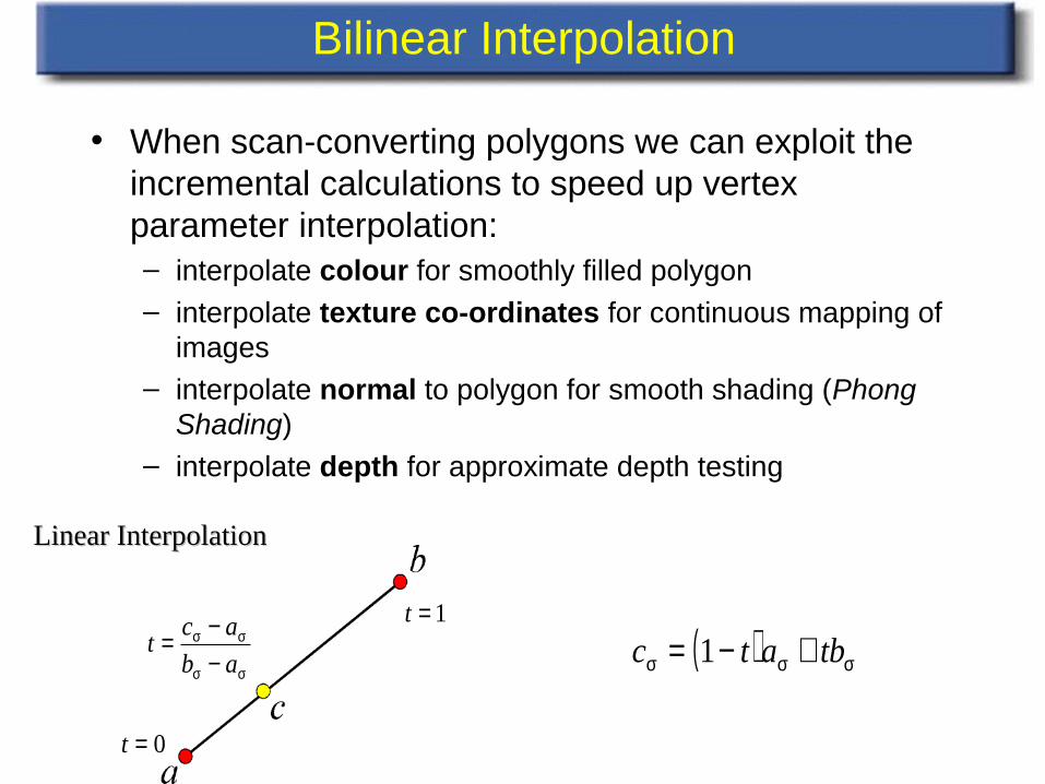
• When scan-converting polygons we can exploit the incremental calculations to speed up vertex parameter interpolation:– interpolate colour for smoothly filled polygon– interpolate texture co-ordinates for continuous mapping of
images– interpolate normal to polygon for smooth shading (Phong
Shading)– interpolate depth for approximate depth testing
Linear InterpolationLinear Interpolation
( ) σσσ +−= tbatc 11=t
0=t
σσ
σσ
−−=
ab
act
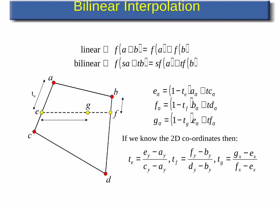
Bilinear Interpolation
( )( )( ) σσσ
σσσ
σσσ
+−=
+−=+−=
tfetg
tdbtf
tcate
g
f
e
1
1
1
( ) ( ) ( )( ) ( ) ( )btfasftbsaf
bfafbaf
+=+⇒+=+⇒
bilinear
linear
If we know the 2D co-ordinates then:
xx
xxg
yy
yyf
yy
yye ef
egt
bd
bft
ac
aet
−−=
−−
=−−
= ,,
te
Bilinear Interpolation
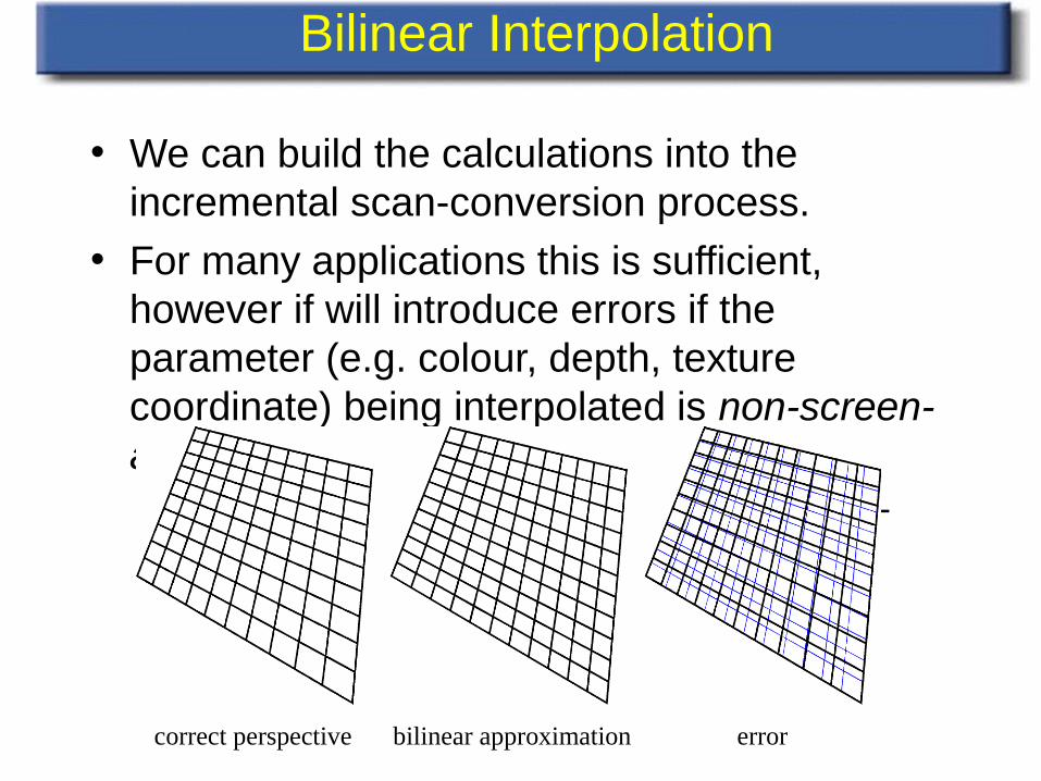
• We can build the calculations into the incremental scan-conversion process.
• For many applications this is sufficient, however if will introduce errors if the parameter (e.g. colour, depth, texture coordinate) being interpolated is non-screen-affine.– distance from viewer, and therefore texture co-
ordinates are non-screen affine:
correct perspective bilinear approximation error
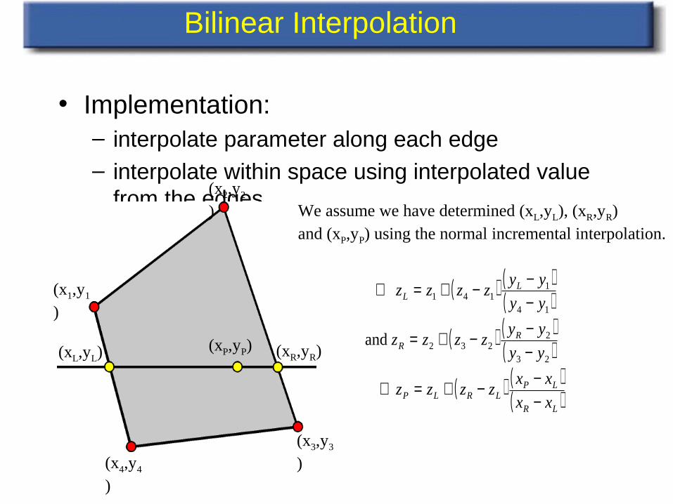
Bilinear Interpolation
• Implementation:– interpolate parameter along each edge– interpolate within space using interpolated value
from the edges
(x4,y4
)
(x1,y1
)
(x3,y3
)
(x2,y2
)
(xL,yL) (xR,yR)(xP,yP)
We assume we have determined (xL,yL), (xR,yR)and (xP,yP) using the normal incremental interpolation.
( ) ( )( )
( ) ( )( )
( ) ( )( )LR
LPLRLP
RR
LL
xx
xxzzzz
yy
yyzzzz
yy
yyzzzz
−−−+=∴
−−−+=
−−−+=⇒
23
2232
14
1141
and
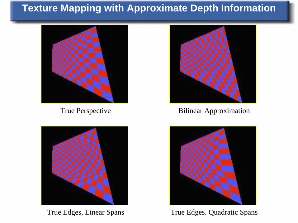
True Perspective
True Edges, Linear Spans True Edges. Quadratic Spans
Bilinear Approximation
Texture Mapping with Approximate Depth Information
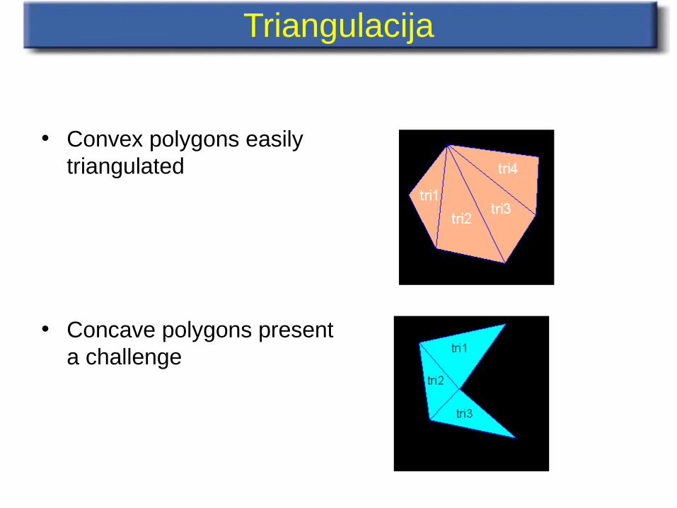
Triangulacija
• Convex polygons easily triangulated
• Concave polygons present a challenge
Rasterizacija trikotnikov
• Interactive graphics hardware commonly uses edge walking or edge equation techniques for rasterizing triangles
Edge Walking
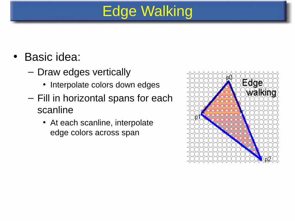
• Basic idea: – Draw edges vertically
• Interpolate colors down edges
– Fill in horizontal spans for each scanline
• At each scanline, interpolate edge colors across span
Edge Walking: Notes
• Order three triangle vertices in x and y– Find middle point in y dimension and compute if it is to the left or
right of polygon. Also could be flat top or flat bottom triangle
• We know where left and right edges are.– Proceed from top scanline downwards– Fill each span– Until breakpoint or bottom vertex is reached
• Advantage: can be made very fast• Disadvantages:
– Lots of finicky special cases
Edge Walking: Disadvantages
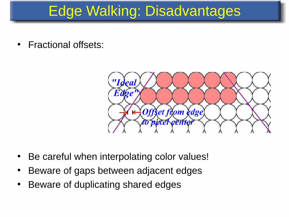
• Fractional offsets:
• Be careful when interpolating color values!• Beware of gaps between adjacent edges• Beware of duplicating shared edges
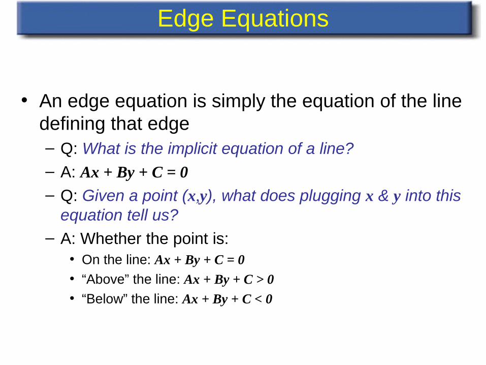
Edge Equations
• An edge equation is simply the equation of the line defining that edge– Q: What is the implicit equation of a line?
– A: Ax + By + C = 0
– Q: Given a point (x,y), what does plugging x & y into this equation tell us?
– A: Whether the point is:• On the line: Ax + By + C = 0
• “Above” the line: Ax + By + C > 0
• “Below” the line: Ax + By + C < 0
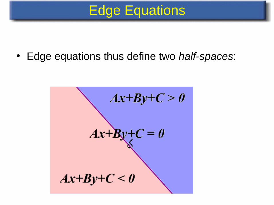
Edge Equations
• Edge equations thus define two half-spaces:
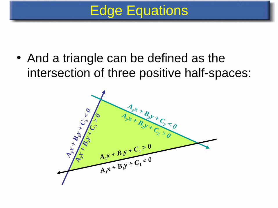
Edge Equations
• And a triangle can be defined as the intersection of three positive half-spaces:
A1x + B1y + C1 < 0
A2 x + B
2 y + C2 < 0
A 3x
+ B 3
y +
C 3 <
0
A1x + B1y + C1 > 0
A 3x
+ B 3
y +
C 3 >
0 A2 x + B
2 y + C2 > 0
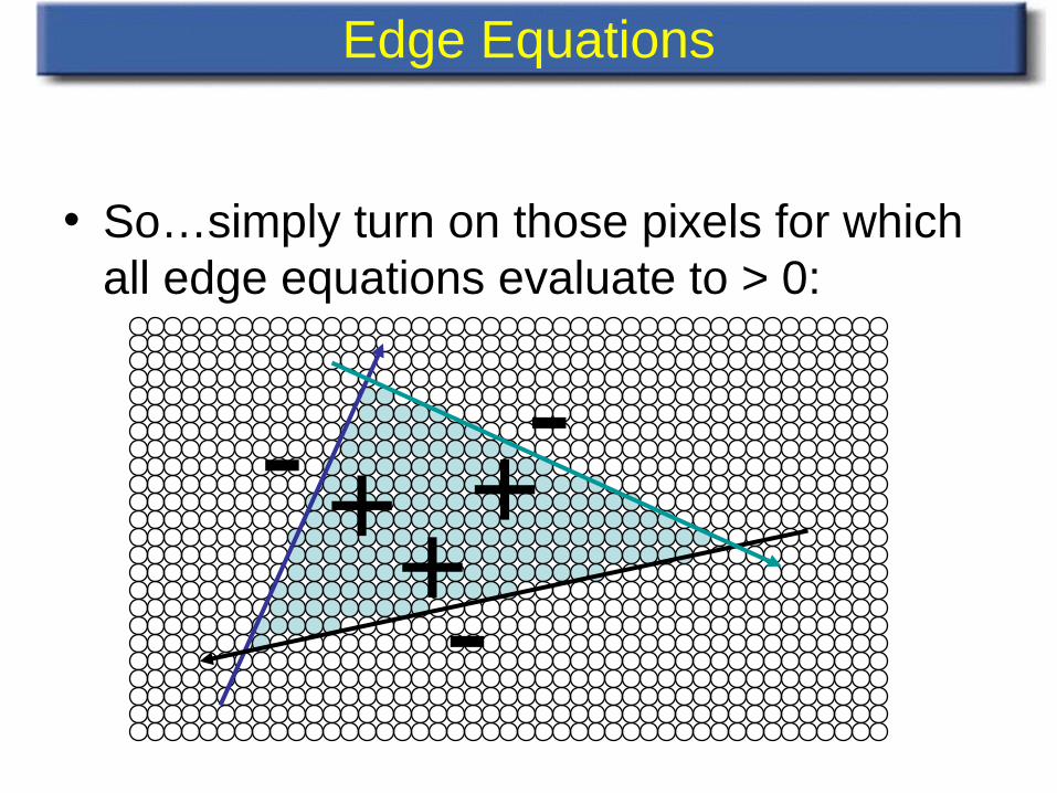
Edge Equations
• So…simply turn on those pixels for which all edge equations evaluate to > 0:
+++
-
--
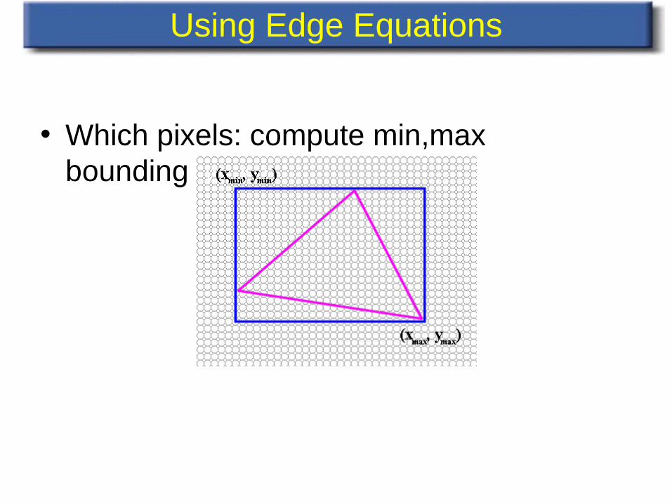
Using Edge Equations
• Which pixels: compute min,max bounding box
• Edge equations: compute from vertices
• Orientation: ensure area is positive (why?)
Computing Edge Equations
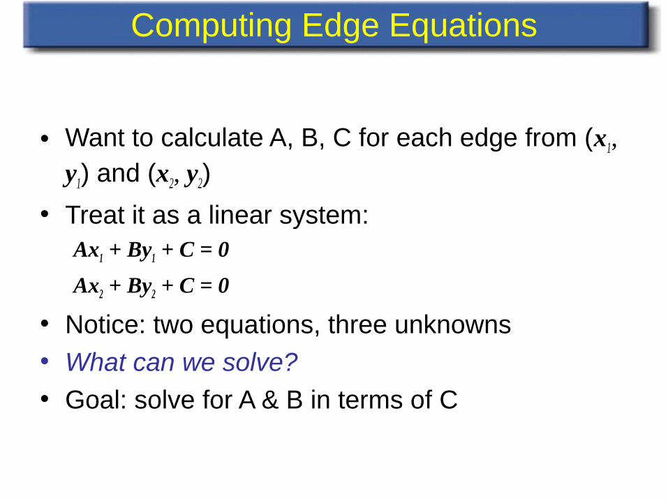
• Want to calculate A, B, C for each edge from (x1, y1) and (x2, y2)
• Treat it as a linear system:Ax1 + By1 + C = 0
Ax2 + By2 + C = 0
• Notice: two equations, three unknowns• What can we solve?• Goal: solve for A & B in terms of C
Computing Edge Equations
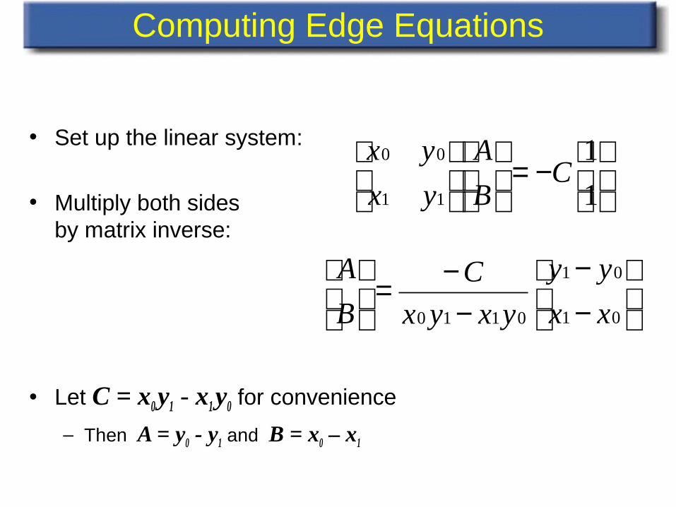
• Set up the linear system:
• Multiply both sidesby matrix inverse:
• Let C = x0 y1 - x1 y0 for convenience
– Then A = y0 - y1 and B = x0 – x1
−=
1
1
11
00C
B
A
yx
yx
−−
−−=
01
01
0110 xx
yy
yxyx
C
B
A
Edge Equations
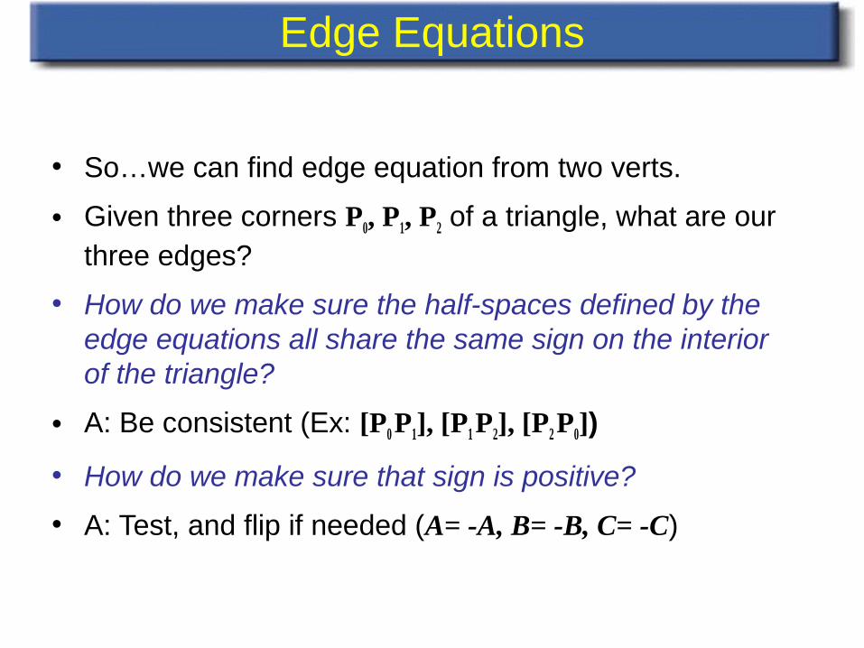
• So…we can find edge equation from two verts.
• Given three corners P0, P1, P2 of a triangle, what are our three edges?
• How do we make sure the half-spaces defined by the edge equations all share the same sign on the interior of the triangle?
• A: Be consistent (Ex: [P0 P1], [P1 P2], [P2 P0])
• How do we make sure that sign is positive?
• A: Test, and flip if needed (A= -A, B= -B, C= -C)
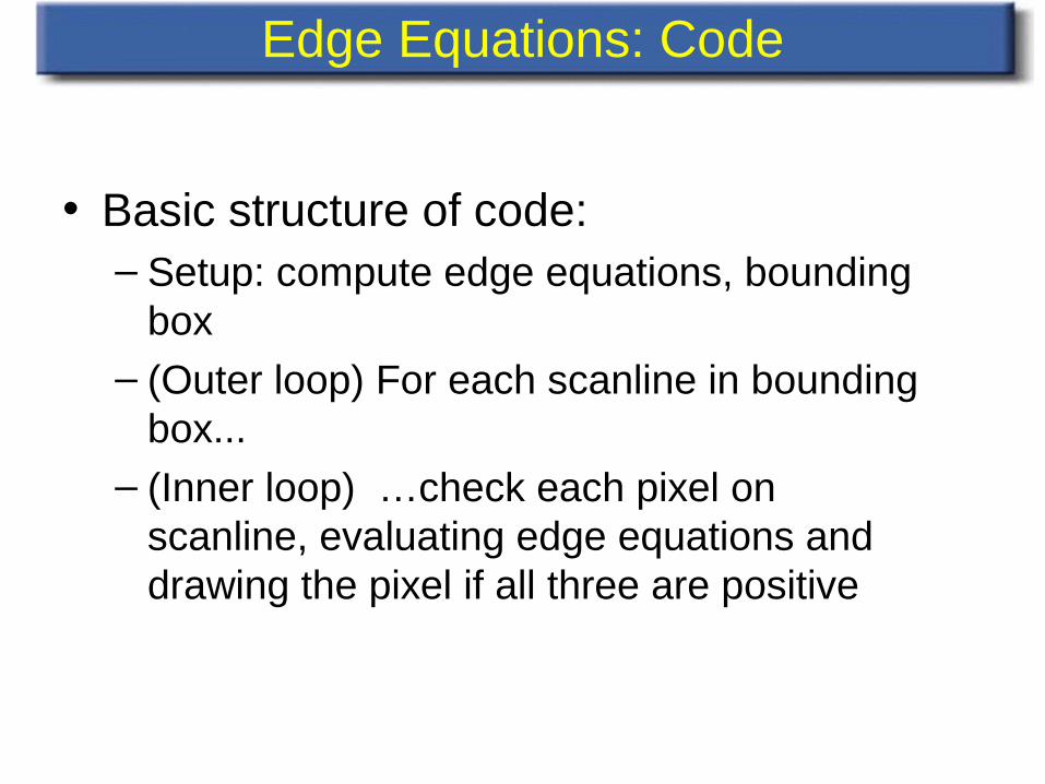
Edge Equations: Code
• Basic structure of code:– Setup: compute edge equations, bounding
box– (Outer loop) For each scanline in bounding
box... – (Inner loop) …check each pixel on
scanline, evaluating edge equations and drawing the pixel if all three are positive
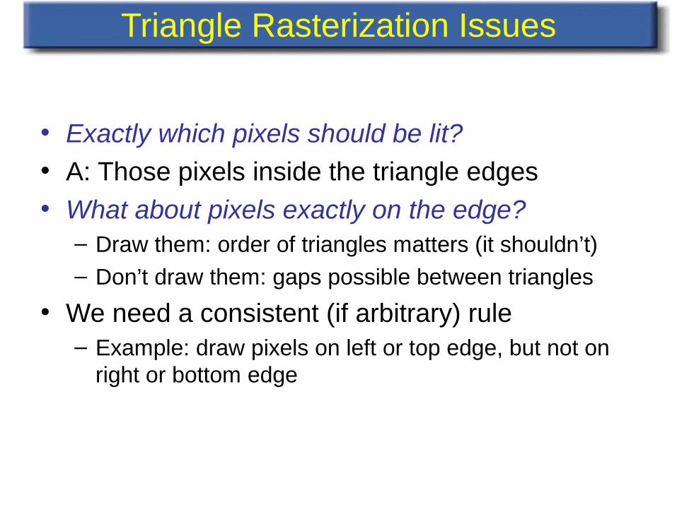
Triangle Rasterization Issues
• Exactly which pixels should be lit?• A: Those pixels inside the triangle edges• What about pixels exactly on the edge?
– Draw them: order of triangles matters (it shouldn’t)– Don’t draw them: gaps possible between triangles
• We need a consistent (if arbitrary) rule – Example: draw pixels on left or top edge, but not on
right or bottom edge
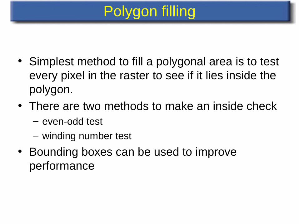
Polygon filling
• Simplest method to fill a polygonal area is to test every pixel in the raster to see if it lies inside the polygon.
• There are two methods to make an inside check– even-odd test
– winding number test
• Bounding boxes can be used to improve performance
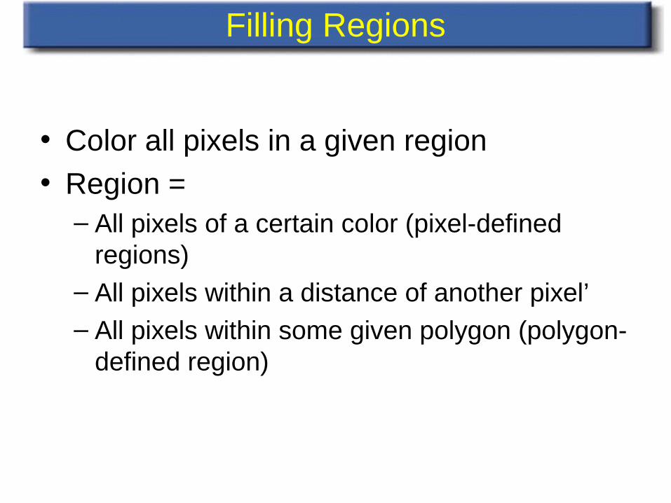
Filling Regions
• Color all pixels in a given region
• Region =– All pixels of a certain color (pixel-defined
regions)– All pixels within a distance of another pixel’– All pixels within some given polygon (polygon-
defined region)
Filling Pixel-defined regions
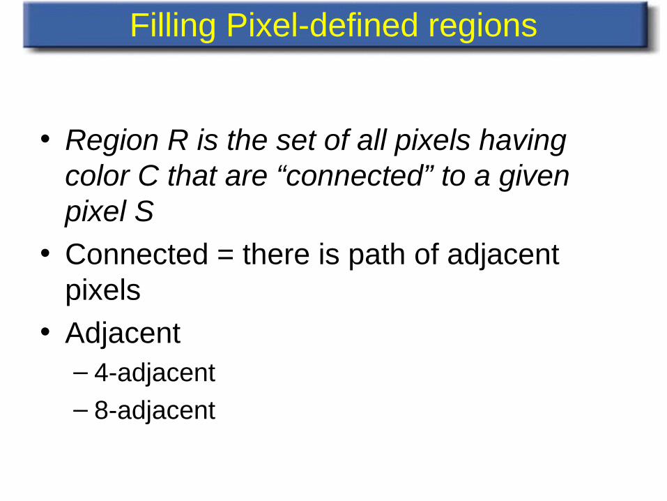
• Region R is the set of all pixels having color C that are “connected” to a given pixel S
• Connected = there is path of adjacent pixels
• Adjacent– 4-adjacent– 8-adjacent
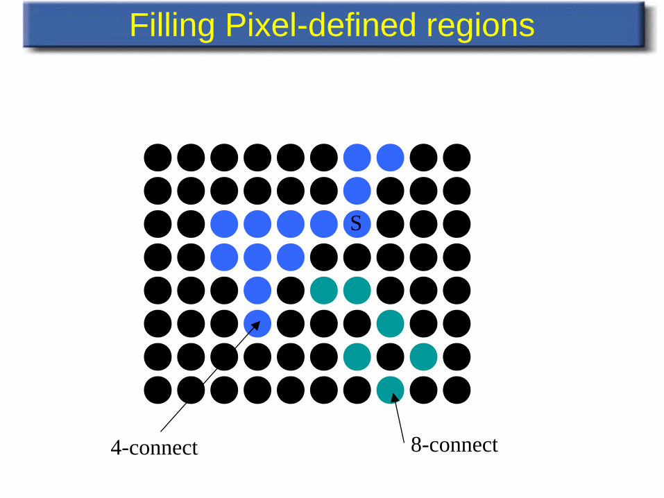
Filling Pixel-defined regions
S
4-connect 8-connect
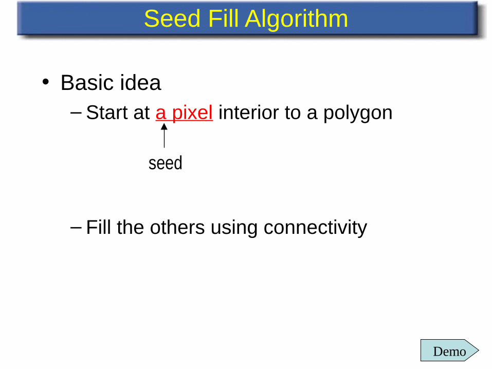
• Basic idea– Start at a pixel interior to a polygon
– Fill the others using connectivity
Seed Fill Algorithm
seed
Demo
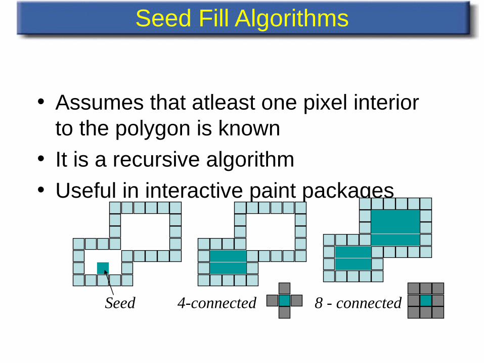
Seed Fill Algorithms
• Assumes that atleast one pixel interior to the polygon is known
• It is a recursive algorithm
• Useful in interactive paint packages
Seed 4-connected 8 - connected
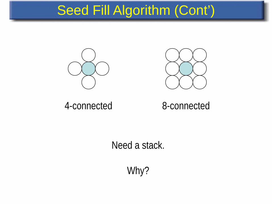
4-connected 8-connected
Need a stack.
Why?
Seed Fill Algorithm (Cont’)
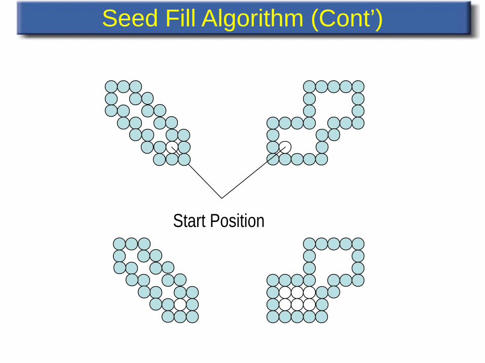
Start Position
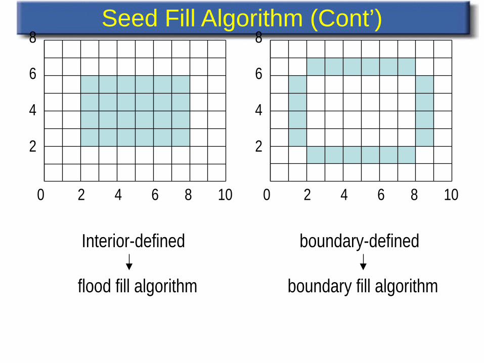
Seed Fill Algorithm (Cont’)
Seed Fill Algorithm (Cont’)
Interior-defined boundary-defined
flood fill algorithm boundary fill algorithm
8
6
4
2
0 2 4 6 8 10 0 2 4 6 8 10
8
6
4
2
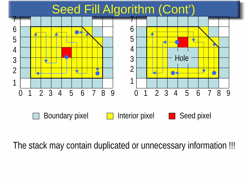
Seed Fill Algorithm (Cont’)
0 1 2 3 4 5 6 7 8 91234567
0 1 2 3 4 5 6 7 8 91234567
Hole
Boundary pixel Interior pixel Seed pixel
The stack may contain duplicated or unnecessary information !!!
Shani, U., “Filling Regions in Binary Raster Images:A Graph-Theoretic Approach”, Computer Graphics,14, (1981), 321-327
Scan Lineconversion
Seedfilling
+
Scan Line Seed Fill
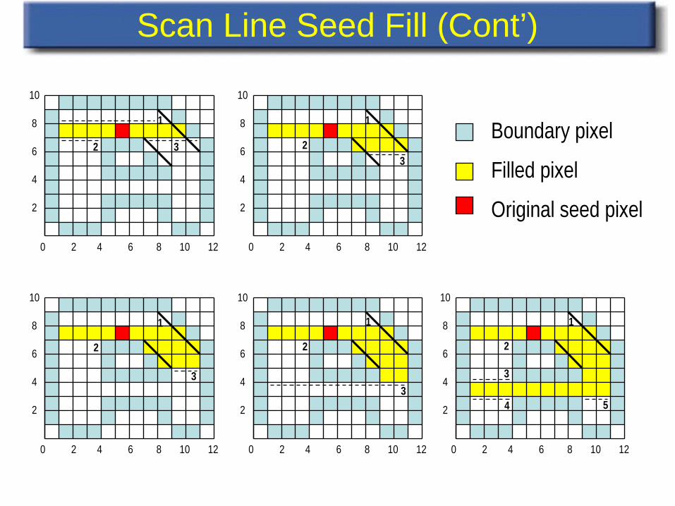
Boundary pixel
Filled pixel
Original seed pixel
1
23
0 2 4 6 8 10 12
10
8
6
4
2
1
2 3
0 2 4 6 8 10 12
10
8
6
4
2
3
1
2
10
8
6
4
2
0 2 4 6 8 10 12
1
2
3
10
8
6
4
2
0 2 4 6 8 10 12
1
2
3
4 5
10
8
6
4
2
0 2 4 6 8 10 12
Scan Line Seed Fill (Cont’)
Filling Pixel-defined regions
• Recursive flood-fill– If a pixel is part of the region, switch its color
– Apply the same procedure to each neighbor
• Neighbor = 4-connect or 8-connect
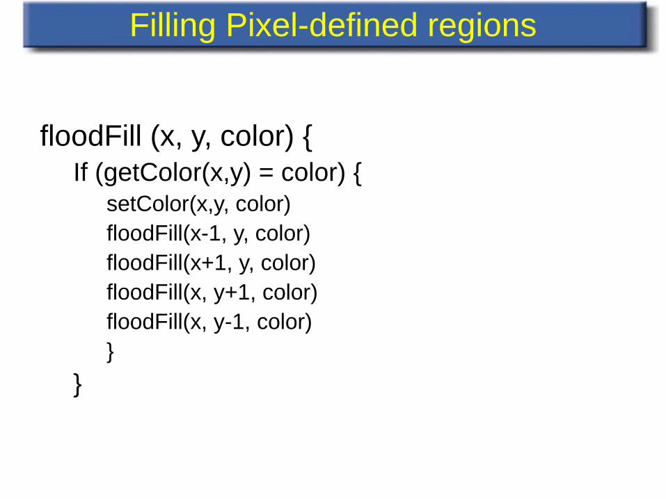
Filling Pixel-defined regions
floodFill (x, y, color) {If (getColor(x,y) = color) {
setColor(x,y, color)floodFill(x-1, y, color)floodFill(x+1, y, color)floodFill(x, y+1, color)floodFill(x, y-1, color)}
}
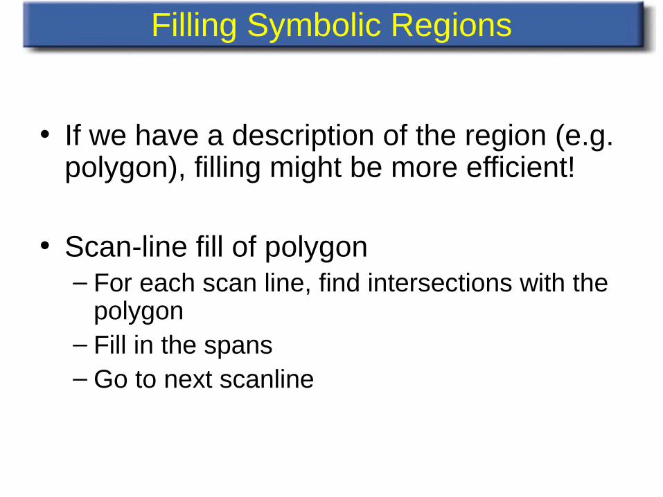
Filling Symbolic Regions
• If we have a description of the region (e.g. polygon), filling might be more efficient!
• Scan-line fill of polygon– For each scan line, find intersections with the
polygon– Fill in the spans– Go to next scanline
How to draw things?
• Given: window on the screen
• Graphics API (e.g. OpenGL) has something of the form:plotPixel(int x, int y)
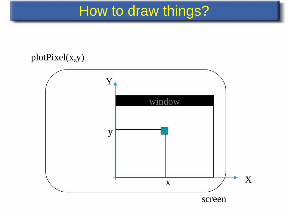
How to draw things?
window
screen
x
y
plotPixel(x,y)
X
Y
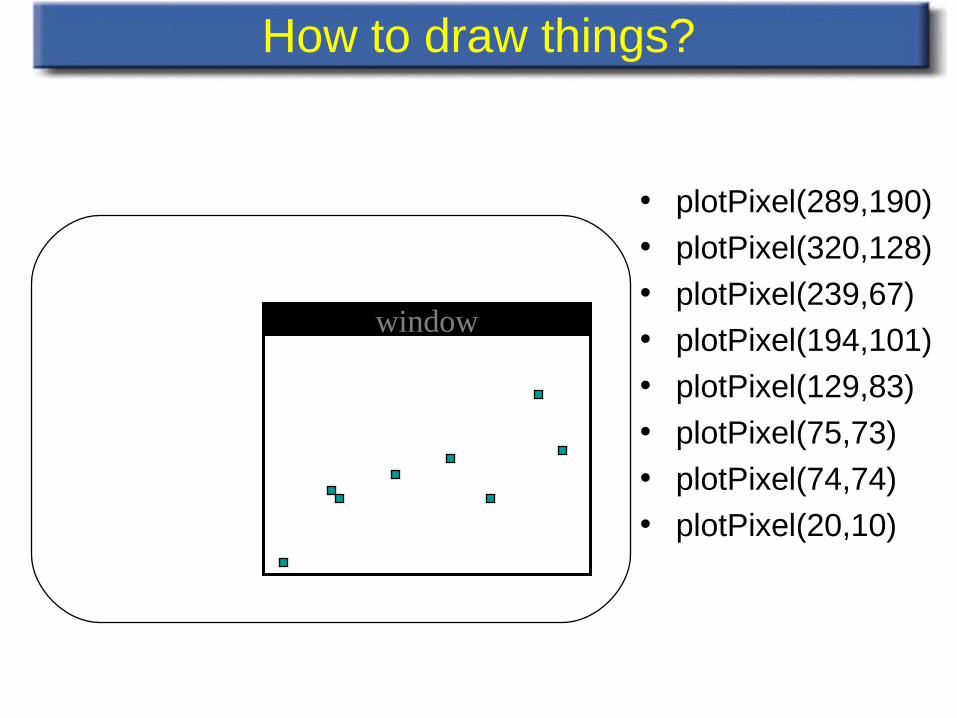
How to draw things?
• plotPixel(289,190)
• plotPixel(320,128)• plotPixel(239,67)• plotPixel(194,101)
• plotPixel(129,83)
• plotPixel(75,73)
• plotPixel(74,74)• plotPixel(20,10)
window
Why is this impractical?
• Coordinates are expressed in screen space, but objects live in (3D) world space
• Resizing window implies we have to change coordinates of objects to be drawn
• We want to make a separation between:– values to describe geometrical objects– values needed to draw these objects on the screen
World window & viewport
• World window:specifies what part of the world should be drawn
• Viewport:rectangular area in the screen window in which we will draw
World window & viewport
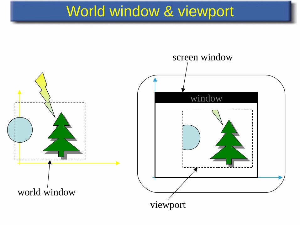
window
viewport
screen window
world window
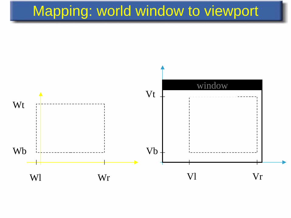
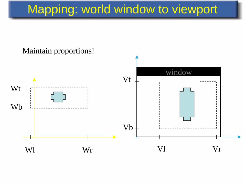
Mapping: world window to viewport
window
Wl Wr
Wb
Wt
Vl Vr
Vb
Vt
Mapping: world window to viewport
window
Wl Wr
Wb
Wt
Vl Vr
Vb
Vt
Maintain proportions!
Mapping: world window to viewport
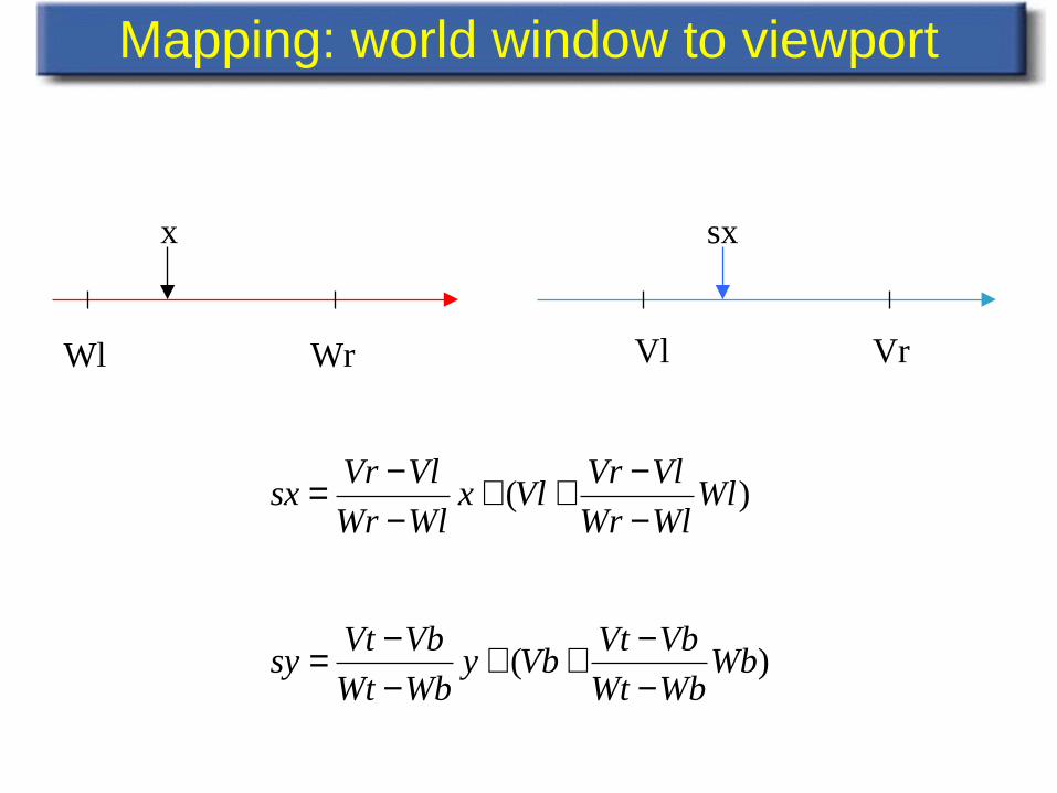
Wl Wr Vl Vr
x sx
)( WlWlWr
VlVrVlx
WlWr
VlVrsx
−−++
−−=
)( WbWbWt
VbVtVby
WbWt
VbVtsy
−−++
−−=
Mapping: world window to viewport
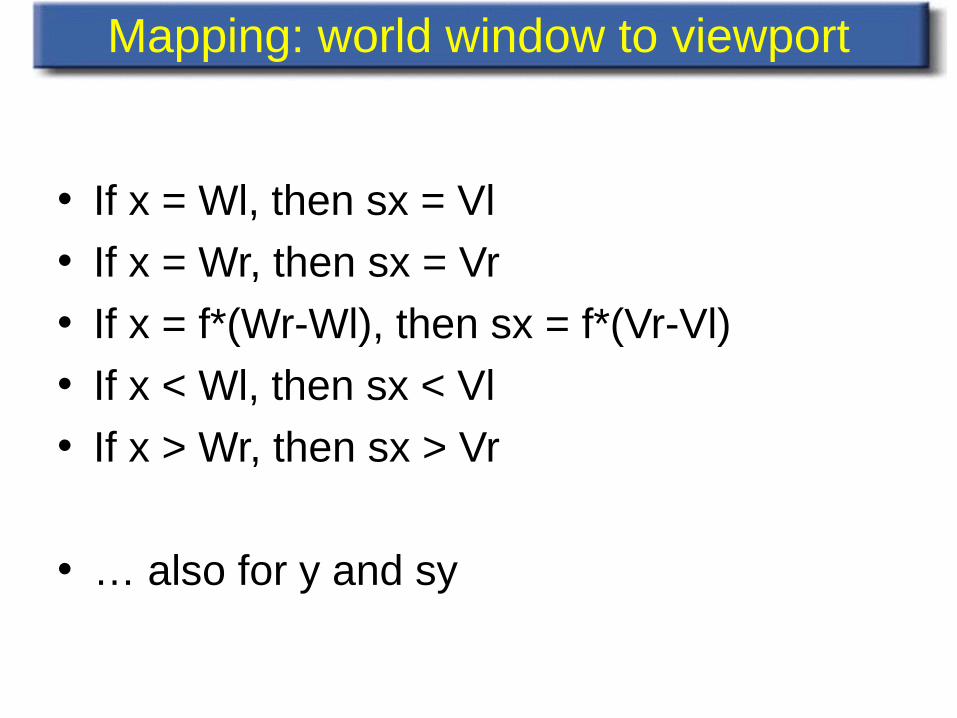
• If x = Wl, then sx = Vl
• If x = Wr, then sx = Vr
• If x = f*(Wr-Wl), then sx = f*(Vr-Vl)
• If x < Wl, then sx < Vl
• If x > Wr, then sx > Vr
• … also for y and sy
World window
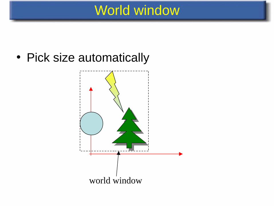
• Pick size automatically
world window
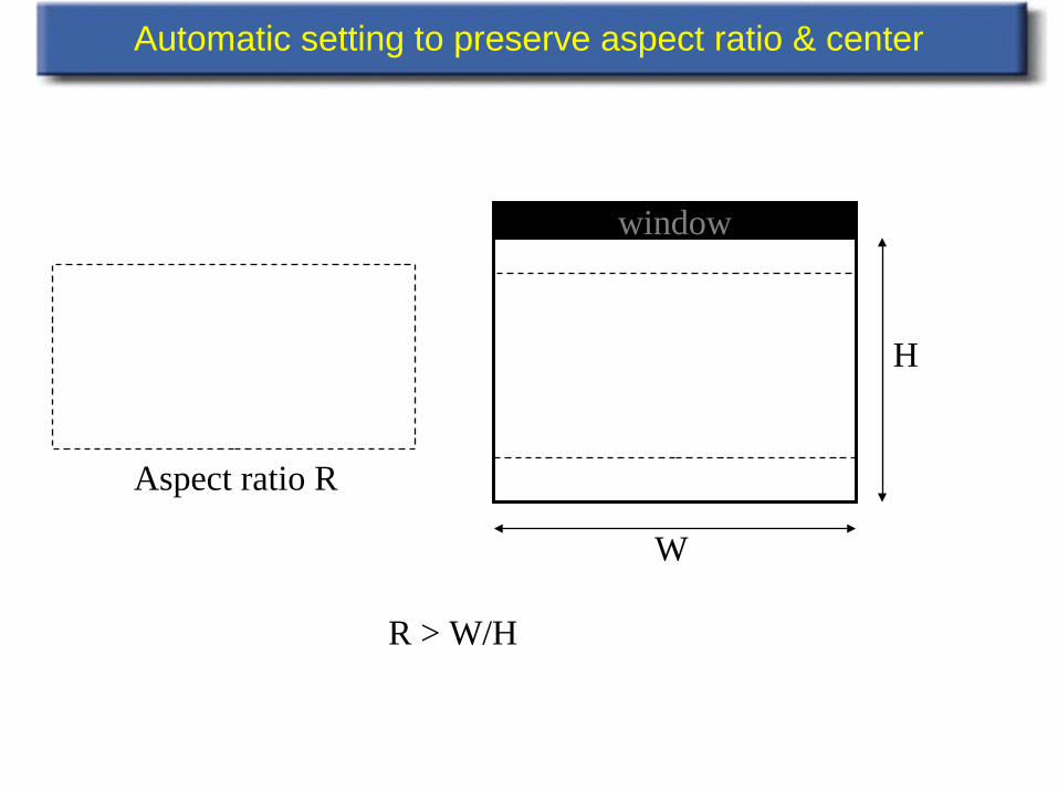
Automatic setting to preserve aspect ratio & center
window
W
H
Aspect ratio R
R > W/H
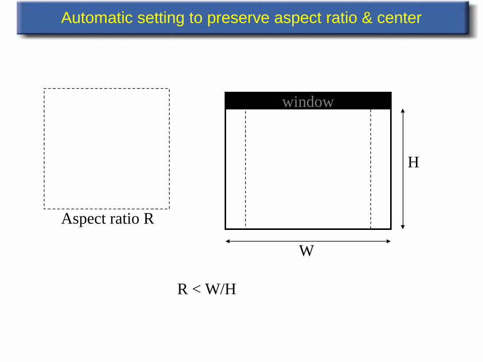
Automatic setting to preserve aspect ratio & center
window
Aspect ratio R
R < W/H
W
H