Algorithms for the Prediction of Coastal CO2

Burke Hales1

Dick Feely2

Ricardo Letelier1

Chris Sabine2

Pete Strutton1

1 Oregon State University2 NOAA Pacific Marine Environmental Laboratory

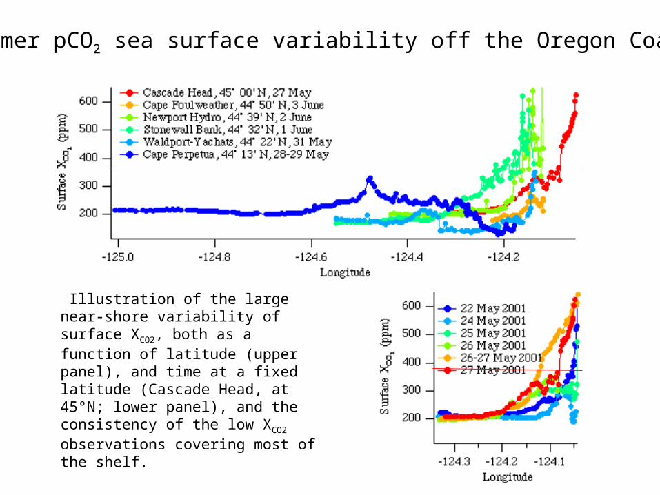
Illustration of the large near-shore variability of surface XCO2, both as a function of latitude (upper panel), and time at a fixed latitude (Cascade Head, at 45°N; lower panel), and the consistency of the low XCO2 observations covering most of the shelf.

Summer pCO2 sea surface variability off the Oregon Coast

- Coastal CO2 data recently compiled.

Integrating fluxes from ‘coastal’ pixels, the bottom line, in Tg C yr-1:Total: +2 ± 35

Mexico: +45 ± 14US: -21 ± 18

Canada: -22 ± 27

LDEO, MBARI, OSU, AOML, UGA databases contain ~106 coastal surface pCO2 measurements dating to 1979 that were excluded from global compilations.

These data were mapped into 1° x 1° pixels within ~3° from the coastline; and monthly-mean fluxes were calculated for each pixel.

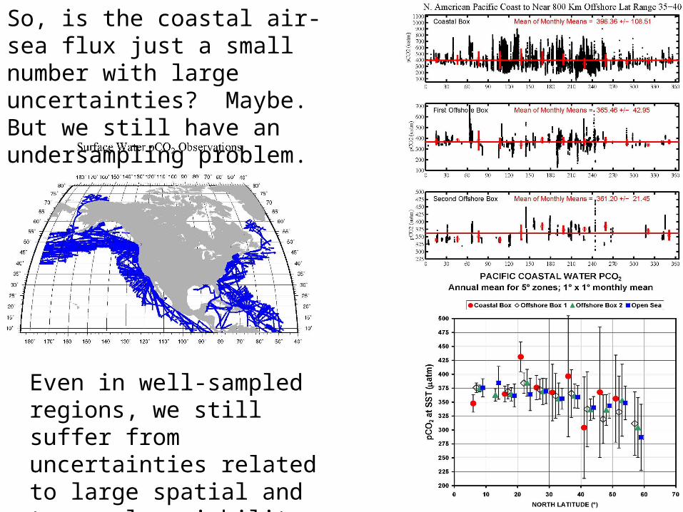
So, is the coastal air-sea flux just a small number with large uncertainties? Maybe. But we still have an undersampling problem.

Even in well-sampled regions, we still suffer from uncertainties related to large spatial and temporal variability, primarily near shore.

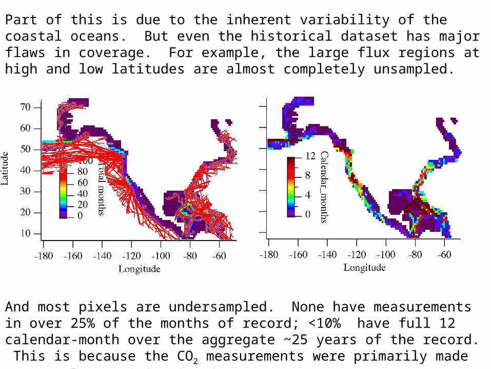
Part of this is due to the inherent variability of the coastal oceans. But even the historical dataset has major flaws in coverage. For example, the large flux regions at high and low latitudes are almost completely unsampled.

And most pixels are undersampled. None have measurements in over 25% of the months of record; <10% have full 12 calendar-month over the aggregate ~25 years of the record. This is because the CO2 measurements were primarily made on vessels participating in open-ocean programs.

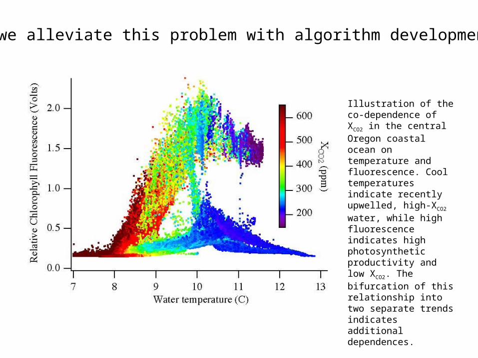
Illustration of the co-dependence of XCO2 in the central Oregon coastal ocean on temperature and fluorescence. Cool temperatures indicate recently upwelled, high-XCO2 water, while high fluorescence indicates high photosynthetic productivity and low XCO2. The bifurcation of this relationship into two separate trends indicates additional dependences.

Can we alleviate this problem with algorithm development?

Early Stages approach:

To date we have included only the following ancillary data in the Coastal CO2 database: Lat, Lon,time, SST, SSS

in an equation of the form:

CO2_mod = A + B*Lat + C*Lon + D*sin(J_Day/365 + E) + F*SST + G*SSS

(This is essentially an MLR, but we are using an algorithm that will allow non-linear functionality)

Complete dataset cannot be even remotely approximated by a single function like the above.

But separating the data into regional subsets holds some promise:

SST Lat, Time

SSTLat, SST

Results show that different regions have different dominant factors driving the algorithms.

But none of the results are very pleasing. The algorithm in general underpredicts the observed range of variability. Some regions have clear subsets of data that have large observed variability for a small range in predicted CO2. Other regions, notably the Pacific, are overall very poorly represented by this algorithm.

-Are higher-order dependences in, er… order?

-Can subsets of the data give better results?

We examined the surface data from the COAST project with an equation of the form:

CO2_mod = A + B*Lat + C*Lon + D*sin(J_Day/365 + E) + F*SST + G*SSS + + H*Chl + I*beam-C + J*Lon*SST

Here, Lon is a good proxy for cross-shelf distance.

The Lon*T term includes some ‘strength of upwelling’ characteristics-- e.g., cool water far from shore represents strong upwelling. It also gives a higher-order dependence on SST.

Depth (m

)

COAST

Coastal Oregon, upwelling season, 2001. Data from cross-shelf transects between 44-45N.

SST, Lon*SST, are most important. Bioptical factors make no improvement in algorithm agreement with observations!

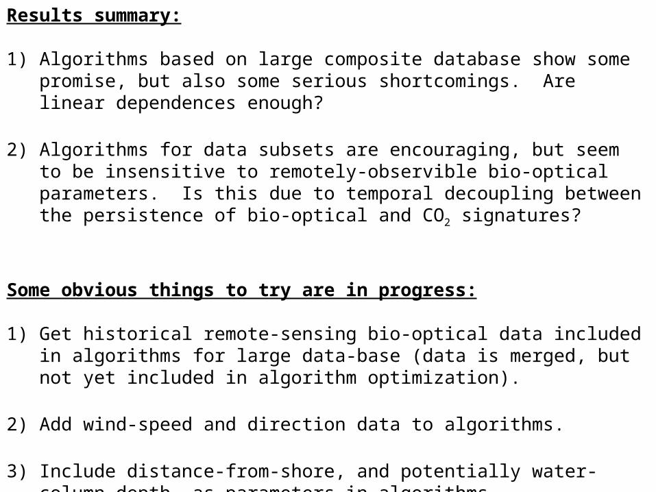
Results summary:

1) Algorithms based on large composite database show some promise, but also some serious shortcomings. Are linear dependences enough?

2) Algorithms for data subsets are encouraging, but seem to be insensitive to remotely-observible bio-optical parameters. Is this due to temporal decoupling between the persistence of bio-optical and CO2 signatures?

Some obvious things to try are in progress:

1) Get historical remote-sensing bio-optical data included in algorithms for large data-base (data is merged, but not yet included in algorithm optimization).

2) Add wind-speed and direction data to algorithms.

3) Include distance-from-shore, and potentially water-column depth, as parameters in algorithms.

4) Assess pCO2 as a function of the time derivative of SST and chl.

Addressing the undersampling problem:

1) A small, low-cost, fast-response system for autonomous surface CO2 and bio-optical measurement has been developed and tested at OSU and will be deployed on the RV Wecoma when she returns from the shipyard in ~weeks.- pCO2 system is centered on a LI-COR 820 IR detector, with a  miniature Liqui-Cel membrane equilibrator and tangential flow filtration.- Optics include chlorophyll and CDOM fluorometry and, initially, beam attenuation.

1) A high-precision traditional CO2 system has been built at PMEL and deployed on the Miller Freeman.

QuickTime™ and aTIFF (Uncompressed) decompressor

are needed to see this picture.

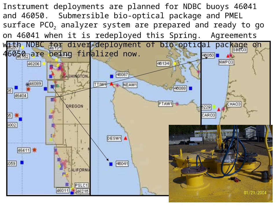
Instrument deployments are planned for NDBC buoys 46041 and 46050. Submersible bio-optical package and PMEL surface PCO2 analyzer system are prepared and ready to go on 46041 when it is redeployed this Spring. Agreements with NDBC for diver-deployment of bio-optical package on 46050 are being finalized now.

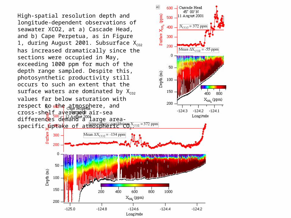
High-spatial resolution depth and longitude-dependent observations of seawater XCO2, at a) Cascade Head, and b) Cape Perpetua, as in Figure 1, during August 2001. Subsurface XCO2 has increased dramatically since the sections were occupied in May, exceeding 1000 ppm for much of the depth range sampled. Despite this, photosynthetic productivity still occurs to such an extent that the surface waters are dominated by XCO2 values far below saturation with respect to the atmosphere, and cross-shelf averaged air-sea differences demand a large area-specific uptake of atmospheric CO2.