Algorithms for Real-Time Object Detection in...

CHAPTER 11

Algorithms for Real-Time Object Detectionin Images

MILOS STOJMENOVIC

11.1 INTRODUCTION

11.1.1 Overview of Computer Vision Applications

The field of Computer Vision (CV) is still in its infancy. It has many real-worldapplications, and many breakthroughs are yet to be made. Most of the companiesin existence today that have products based on CV can be divided into three maincategories: auto manufacturing, computer circuit manufacturing, and face recognition.There are other smaller categories of this field that are beginning to be developedin industry such as pharmaceutical manufacturing applications and traffic control.Auto manufacturing employs CV through the use of robots that put the cars together.Computer circuit manufacturers use CV to visually check circuits in a production lineagainst a working template of that circuit. CV is used as quality control in this case. Thethird most common application of CV is in face recognition. This field has becomepopular in the last few years with the advent of more sophisticated and accuratemethods of facial recognition. Applications of this technology are used in securitysituations like checking for hooligans at sporting events and identifying known thievesand cheats in casinos. There is also the related field of biometrics where retinalscans, fingerprint analysis, and other identification methods are conducted using CVmethods.

Traffic control is also of interest because CV software systems can be applied toalready existing hardware in this field. By traffic control, we mean the regulationor overview of motor traffic by means of the already existing and functioning arrayof police monitoring equipment. Cameras are already present at busy intersections,highways, and other junctions for the purposes of regulating traffic, spotting problems,and enforcing laws such as running red lights. CV could be used to make all of thesetasks automatic.

Handbook of Applied Algorithms: Solving Scientific, Engineering and Practical ProblemsEdited by Amiya Nayak and Ivan Stojmenovic Copyright © 2008 John Wiley & Sons, Inc.

315

316 ALGORITHMS FOR REAL-TIME OBJECT DETECTION IN IMAGES

11.2 MACHINE LEARNING IN IMAGE PROCESSING

AdaBoost and support vector machines (SVMs) are, among others, two very pop-ular and conceptually similar machine learning tools for image processing. Theyare both based on finding a set of hyperplanes to separate the sets of positive andnegative examples. Current image processing culture involving machine learningfor real-time performance almost exclusively uses AdaBoost instead of SVMs. Ad-aBoost is easier to program and has proven itself to work well. There are veryfew papers that deal with real-time detection using SVM principles. This makesthe AdaBoost approach a better choice for real-time applications. A number ofrecent papers, using both AdaBoost and SVMs, confirm the same, and even ap-ply a two-phase process. Most windows are processed in the first phase by Ad-aBoost, and in the second phase, an SVM is used on difficult cases that couldnot be easily eliminated by AdaBoost. This way, the real-time constraint remainsintact.

Le and Satoh [16] maintain that “The pure SVM has constant running time of 554windows per second (WPS) regardless of complexity of the input image, the pure Ad-aBoost (cascaded with 37 layers—5924 features) has running time of 640, 515 WPS.”If a pure SVM approach was applied to our test set, it would take 17, 500, 000/554 ≈ 9h of pure run time to test the 106 images. It would take roughly 2 min to process animage of size 320× 240. Thus, Lee and Satoh [16] claim that cascaded AdaBoost is1000 times faster than SVMs. A regular AdaBoost with 30 features was presented inthe works by Stojmenovic [24,25]. A cascaded design cannot speed up the describedversion by more than 30 times. Thus, the program in the works by Stojmenovic [24,25]is faster than SVM by over 1000/30 > 30 times.

Bartlett et al. [3] used both AdaBoost and SVMs for their face detection and facialexpression recognition system. Although they state that “AdaBoost is significantlyslower to train than SVMs,” they only use AdaBoost for face detection, and it isbased on Viola and Jones’ approach [27]. For the second phase, facial expressionrecognition on detected faces, they use three approaches: AdaBoost, SVMs, and acombined one (all applied on Gabor representation), and reported differences within3 percent of each other. They gave a simple explanation for choosing AdaBoost in theface detection phase, “The average number of features that need to be evaluated foreach window is very small, making the overall system very fast” [3]. Moreover, each ofthese features is evaluated in constant time, because of integral image preprocessing.That performance is hard to beat, and no other approach in image processing literaturefor real-time detection is seriously considered now.

AdaBoost was proposed by Freund and Schapire [8]. The connection betweenAdaBoost and SVMs was also discussed by them [9]. They even described two verysimilar expressions for both of them, where the difference was that the Euclideannorm was used by SVMs while the boosting process used Manhattan (city block) andmaximum difference norms. However, they also list several important differences.Different norms may result in very different margins. A different approach is usedto efficiently search in high dimensional spaces. The computation requirements aredifferent. The computation involved in maximizing the margin is mathematical pro-

MACHINE LEARNING IN IMAGE PROCESSING 317

gramming, that is, maximizing a mathematical expression given a set of inequalities.The difference between the two methods in this regard is that SVM corresponds toquadratic programming, while AdaBoost corresponds only to linear programming[9]. Quadratic programming is more computationally demanding than linear program-ming [9].

AdaBoost is one of the approaches where a “weak” learning algorithm, whichperforms just slightly better than random guessing, is “boosted” into an arbitrarilyaccurate “strong” learning algorithm. If each weak hypothesis is slightly better thanrandom, then the training error drops exponentially fast [9]. Compared to other similarlearning algorithms, AdaBoost is adaptive to the error rates of the individual weakhypotheses, while other approaches required that all weak hypotheses need to haveaccuracies over a parameter threshold. It is proven [9] that AdaBoost is indeed aboosting algorithm in the sense that it can efficiently convert a weak learning algorithminto a strong learning algorithm (which can generate a hypothesis with an arbitrarilylow error rate, given sufficient data).

Freund and Schapire [8] state “Practically, AdaBoost has many advantages. It isfast, simple, and easy to program. It has no parameters to tune (except for the numberof rounds). It requires no prior knowledge about the weak learner and so can beflexibly combined with any method for finding weak hypotheses. Finally, it comeswith a set of theoretical guarantees given sufficient data and a weak learner that canreliably provide only moderately accurate weak hypotheses. This is a shift in mindset for the learning-system designer: instead of trying to design a learning algorithmthat is accurate over the entire space, we can instead focus on finding weak learningalgorithms that only need to be better than random. On the other hand, some caveatsare certainly in order. The actual performance of boosting on a particular problem isclearly dependent on the data and the weak learner. Consistent with theory, boostingcan fail to perform well given insufficient data, overly complex weak hypotheses, orweak hypotheses that are too weak. Boosting seems to be especially susceptible tonoise.”

Schapire and Singer [23] described several improvements to Freund and Schapire’s[8] original AdaBoost algorithm, particularly in a setting in which hypotheses mayassign confidences to each of their predictions. More precisely, weak hypotheses canhave a range over all real numbers rather than the restricted range [−1,+1] assumedby Freund and Schapire [8]. While essentially proposing a general fuzzy AdaBoosttraining and testing procedure, Howe and Coworkers [11, 34] do not describe any spe- [Q1]

cific variant, with concrete fuzzy classification decisions. We propose in this chapter aspecific variant of fuzzy AdaBoost. Whereas Freund and Schapire [8] prescribe a spe-cific choice of weights for each classifier, Schapire and Singer [23] leave this choiceunspecified, with various tunings. Extensions to multiclass classifications problemsare also discussed.

In practice, the domain of successful applications of AdaBoost in image processingis any set of objects that are typically seen from the same angle and have a constantorientation. AdaBoost can successfully be trained to identify any object if this object isviewed from an angle similar to that in the training set. Practical real-world examplesthat have been considered so far include faces, buildings, pedestrians, some animals,


and cars. The backbone of this research comes from the face detector work done byViola et al. [27]. All subsequent papers that use and improve upon AdaBoost areinspired by it.

11.3 VIOLA AND JONES’ FACE DETECTOR

The face detector proposed by Viola and Jones [27] was the inspiration for all otherAdaBoost applications thereafter. It involves different stages of operation. The trainingof the AdaBoost machine is the first part and the actual use of this machine is thesecond part. Viola and Jones’ contributions come in the training and assembly of theAdaBoost machine. They had three major contributions: integral images, combiningfeatures to find faces in the detection process, and use of a cascaded decision processwhen searching for faces in images. This machine for finding faces is called cascadedAdaBoost by Viola and Jones [27]. Cascaded AdaBoost is a series of smaller AdaBoostmachines that together provide the same function as one large AdaBoost machine,yet evaluate each subwindow more quickly, which results in real-time performance.To understand cascaded AdaBoost, regular AdaBoost will have to be explained first.The following sections will describe Viola and Jones’ face detector in detail.

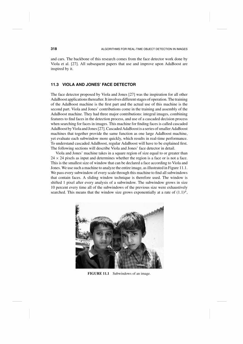
Viola and Jones’ machine takes in a square region of size equal to or greater than24× 24 pixels as input and determines whether the region is a face or is not a face.This is the smallest size of window that can be declared a face according to Viola andJones. We use such a machine to analyze the entire image, as illustrated in Figure 11.1.We pass every subwindow of every scale through this machine to find all subwindowsthat contain faces. A sliding window technique is therefore used. The window isshifted 1 pixel after every analysis of a subwindow. The subwindow grows in size10 percent every time all of the subwindows of the previous size were exhaustivelysearched. This means that the window size grows exponentially at a rate of (1.1)p,

FIGURE 11.1 Subwindows of an image.

VIOLA AND JONES’ FACE DETECTOR 319

where p is the number of scales. In this fashion, more than 90 percent of faces of allsizes can be found in each image.

As with any other machine learning approach, the machine must be trained usingpositive and negative examples. Viola and Jones used 5000 positive examples ofrandomly found upright, forward-facing faces and 10,000 negative examples of anyother nonface objects as their training data. The machine was developed by trying tofind combinations of common attributes, or features of the positive training set thatare not present in the negative training set.

The library of positive object (head) representatives contains face pictures thatare concrete examples. That is, faces are cropped from larger images, and positiveexamples are basically closeup portraits only. Moreover, positive images should beof the same size (that is, when cut out of larger images, they need to be scaled so thatall positive images are of the same size). Furthermore, all images are frontal uprightfaces. The method is not likely to work properly if the faces change orientation.

11.3.1 Features

An image feature is a function that maps an image into a number or a vector (array).Viola and Jones [27] used only features that map images into numbers. Moreover, theyused some specific types of features, obtained by selecting several rectangles withinthe training set, finding the sum of pixel intensities in each rectangle, assigning apositive or negative sign and/or weight to each sum, and then summing them. Thepixel measurements used by Viola and Jones were the actual grayscale intensities ofpixels. If the areas of the dark (positive sign) and light (negative sign) regions are notequal, the weight of the lesser region is raised. For example, feature 2.1 in Figure 11.2has a twice greater light area than a dark one. The area of the dark rectangle in this casewould be multiplied by 2 to normalize the feature. The main problem is to find whichof these features, among the thousands available, would best distinguish positive andnegative examples, and how to combine them into a learning machine.

Figure 11.2 shows the set of basic shapes used by Viola and Jones [27]. Addingfeatures to the feature set can increase the accuracy of the AdaBoost machine at thecost of additional training time. Each of the shapes seen in Figure 11.2 is scaled andtranslated anywhere in the test images, consequently forming features. Therefore,each feature includes a basic shape (as seen in Fig. 11.2), its translated position in theimage, and its scaling factors (height and width scaling). These features define theseparating ability between positive and negative sets. This phenomenon is illustratedin Figure 11.3. Both of the features seen in Figure 11.3 (each defined by its positionand scaling factors) are derived from the basic shapes in Figure 11.2.

FIGURE 11.2 Basic shapes that generate features by translation and scaling.


FIGURE 11.3 First and second features in Viola and Jones face detection.

Figure 11.3 shows the first and second features selected by the program [27]. Whyare they selected? The first feature shows the difference in pixel measurements forthe eye area and area immediately below it. The “black” rectangle covering the eyesis filled with predominantly darker pixels, whereas the area immediately beneath theeyes is covered with lighter pixels. The second feature also concentrates on the eyes,showing the contrast between two rectangles containing eyes and the area betweenthem. This feature corresponds to feature 2.1 in Figure 11.2 where the light and darkareas are inverted. This is not a separate feature; it was drawn this way in Figure 11.3to better depict the relatively constant number obtained by this feature when it isevaluated in this region on each face.

11.3.2 Weak Classifiers (WCs)

A WC is a function of the form h(x, f, s, θ), where x is the tested subimage, f is thefeature used, s is the sign (+ or −), and θ is the threshold. The sign s defines onwhat side of the threshold the positive examples are located. Threshold θ is usedto establish whether a given image passes a classifier test in the following fashion:when feature f is evaluated on image x, the resulting number is compared to thresholdθ to determine how this image is categorized by the given feature. The equation isgiven as sf (x)<sθ. If the equation evaluates true, the image is classified as positive.The function h(x, f, s, θ) is then defined as follows: h(x, f, s, θ) = 1 if sf (x) < sθ

and 0 otherwise. This is expected to correspond to positive and negative examples,respectively. There are a few ways to determine the threshold θ. In the followingexample, the green numbers are considered to be the positive set, and the red lettersare considered to be the negative set. The threshold is set to be the black vertical lineafter the “7” since at this location overall classification error is minimal. All of thepositions are tried, and the one with minimal error is selected. The error function thatis used is the number of misclassifications divided by the total number of examples.The array of evaluated feature values is sorted by the values of f (x), and it showspositive examples as 1, 2, 3, . . . in green and negatives as A, B, C, D, . . . in red. Theerror of the threshold selected below is 3/17 ≈ 0.17.


In general, the threshold is found to be the value θ that best separates the positiveand negative sets. When a feature f is selected as a “good” distinguisher of imagesbetween positive and negative sets, its value would be similar for images in the positiveset and different for all other images. When this feature is applied to an individualimage, a number f (x) is generated. It is expected that values f (x) for positive andnegative images can be separated by a threshold value of θ.

It is worthy to note that a single WC needs only to produce results that are slightlybetter than chance to be useful. A combination of WCs is assembled to produce astrong classifier as seen in the following text.

11.3.3 Strong Classifiers

A strong classifier is obtained by running the AdaBoost machine. It is a linear com-bination of WCs. We assume that there are T WCs in a strong classifier, labelledh1, h2, . . . , hT , and each of these comes with its own weight labeled α1, α2, . . . , αT .Tested image x is passed through the succession of WCs h1(x), h2(x), . . . , hT (x), andeach WC assesses if the image passed its test. The assessments are discrete values:hi(x) = 1 for a pass and hi(x) = 0 for a fail. αi(x) are in the range [0,+∞]. Notethat hi(x) = hi(x, fi, si, θi) is abbreviated here for convenience. The decision thatclassifies an image as being positive or negative is made by the following inequality:

α1h1(x)+ α2h2(x)+ . . .+ αT hT (x) > α/2 where α =T∑

i=1

αi.

From this equation, we see that images that pass a weighted average of half of theWC tests are cataloged as positive. It is therefore a weighted voting of selected WCs.

11.3.4 AdaBoost: Meta Algorithm

In this section we explain the general principles of the AdaBoost (an abbreviation ofAdaptive Boosting) learning strategy [8]. First, a huge (possibly hundreds of thou-sands) “panel” of experts is identified. Each expert, or WC, is a simple threshold-based decision maker, which has a certain accuracy. The AdaBoost algorithm willselect a small panel of these experts, consisting of possibly hundreds of WCs, eachwith a weight that corresponds to its contribution in the final decision. The expertiseof each WC is combined in a classifier so that more accurate experts carry moreweight.

The selection of WCs for a classifier is performed iteratively. First, the best WCis selected, and its weight corresponds to its overall accuracy. Iteratively, the algo-rithm identifies those records in the training data that the classifier built so far wasunable to capture. The weights of the misclassified records increase since it becomesmore important to correctly classify them. Each WC might be adjusted by chang-ing its threshold to better reflect the new weights in the training set. Then a singleWC is selected, whose addition to the already selected WCs will make the greatestcontribution to improving the classifier’s accuracy. This process continues iteratively


until a satisfactory accuracy is achieved, or the limit for the number of selected WCsis reached. The details of this process may differ in particular applications, or inparticular variants of the AdaBoost algorithm.

There exist several AdaBoost implementations that are freely available inWeka (Java-based package http://www.cs.waikato.ac.nz/ml) and in R (http://www.r-project.org). Commercial data mining toolkits that implement AdaBoost includeTreeNet, Statistica, and Virtual Predict. We did not use any of these packages fortwo main reasons. First, our goal was to achieve real-time performance, which re-stricted the choice of programming languages. Next, we have modified the generalalgorithm to better suit our needs, which required us to code it from scratch.

AdaBoost is a general scheme adaptable to many classifying tasks. Little is as-sumed about the learners (WCs) used. They should merely perform only a little betterthan random guesses in terms of error rates. If each WC is always better than a chance,then AdaBoost can be proven to converge to a perfectly accurate classifier (no train-ing error). Boosting can fail to perform if there is insufficient data or if WCs areoverly complex. It is also susceptible to noise. Even when the same problem is beingsolved by different people applying AdaBoost, the performance greatly depends onthe training set being selected and the choice of WCs (that is, features).

In the next subsection, the details of the AdaBoost training algorithm, as used byViola and Jones [27], will be given. In this approach, positive and negative trainingsets are separated by a cascade of classifiers, each constructed by AdaBoost. Realtime performance is achieved by selecting features that can be computed in constanttime. The training time of the face detector appears to be slow, even taking monthsaccording to some reports. Viola and Jones’ face finding system has been modifiedin literature in a number of articles. The AdaBoost machine itself was modified inliterature in several ways.

11.3.5 AdaBoost Training Algorithm

We now show how to create a classifier with the AdaBoost machine. It follows thealgorithm given in the work by Viola and Jones [27]. The machine is given images(x1, y1), . . . , (xq, yq) as input, where yi = 1 or 0 for positive and negative examples,respectively. In iteration t, the ith image is assigned the weight w(t, i), which corre-sponds to the importance of that image for a good classification. The initial weights arew(1, i) = 1/(2p), 1/(2n), for yi = 0 or 1, respectively, where n and p are the numbersof negatives and positives, respectively, q = p+ n. That is, all positive images haveequal weight, totaling 1

2 , and similarly for all negative images. The algorithm willselect, in step t, the tth feature f, its threshold value θ, and its direction of inequalitys(s = 1 or − 1). The classification function is h(x, f, s, θ) = 1 (declared positive) ifsf (x)<sθ, and 0 otherwise (declared negative).

The expression |h(xi, f, s, θ)− yi| indicates whether or not h(x, f, s, θ) correctlyclassified image xi. Its value is 0 for correct classification, and 1 for incorrect clas-sification. The sum

∑Ni=1 w(t, i)× |h(xi, f, s, θ)− yi| then represents the weighted

misclassification error when using h(x, f, s, θ) as the feature-based classifier. Thegoal is to minimize that sum when selecting the next WC.


We revisit the classification of numbers and letters example to illustrate the as-signment of weights in the training procedure. We assume that feature 1 classifies theexample set in the order seen below. The threshold is chosen to be just after the “7”since this position minimizes the classification error. We will call the combination offeature 1 with its threshold WC 1. We notice that “I”, “9,” and “2” were incorrectlyclassified. The number of incorrect classifications determines the weight α1 of thisclassifier. The fewer errors that it makes, the heavier the weight it is awarded.

The weights of the incorrectly classified examples (I, 9, and 2) are increased beforefinding the next feature in an attempt to find a feature that can better classify casesthat are not easily sorted by previous features. We assume that feature two orders theexample set as seen below.

Setting the threshold just after the “2” minimizes the error in classification. Wenotice that this classifier makes more mistakes in classification than its predecessor.This means that its weight, α2, will be less that α1. The weights for elements “E”, “I,”“8,” and “4” are increased. These are the elements that were incorrectly classified byWC 2. The actual training algorithm will be described in pseudocode below.

For t=1 to T do:

Normalize the weights w(t, i), by dividing each of them with their sum (so thatthe new sum of all weights becomes 1);

swp← sum of weights of all positive imagesswn← sum of weights of all negative images(* note that swp+ swn = 1 *)

FOR each candidate feature f, find f (xi) and w(t, i)∗f (xi), i = 1, . . . , q.

- Consider records (f (xi), yi, w(t, i)). Sort these records by the f (xi) fieldwith mergesort, in increasing order. Let the obtained array of the f (xi)field be g1, g2, . . . , gq. The corresponding records are (gj, status(j), w′(j)) =(f (xi), yi, w(t, i)), where gj = f (xi). That is, if the jth element gj is equal to ithelement from the original array f (xi) then status(j) = yi and w′(j) = w(t, i).

(*Scan through the sorted list, looking for threshold θ and direction s that mini-mizes the error e(f, s, θ)∗)

sp← 0; sn← 0; (*weight sums for positives/negatives below a consideredthreshold *)

emin← minimal total weighted classification errorIf swn<swp then {emin← swn; smin← 1; θmin← gn + 1 (*all declared

positive*)


else { emin← swp; smin← 1; θmin← g1 − 1 } (*all declared negative*)

For j← 1 to q-1 do {If status(j) = 1 then sp← sp+ w′(j) else sn← sn+ w′(j)θ← (gj + gj+1)/2If sp+ swn− sn<emin then {emin← sp+ swn− sp; smin←−1; θmin← θ }If sn+ swp− sp<emin then {emin← sn+ swp− sp; smin← 1; θmin←θ } }

EndFOR

Set st ← smin; set θt ← θmin(*s and θ of current stage are determined*)βt ← emin/(1− emin);αT ←−log(βt) (* αT is the output of AdaBoost for the second part*)

Update the weights for the next weak classifier, if needed:

w(t+ 1, i)←w(t, i)β1−et , where e=

{0 if xiis correctly classified bycurrent ht1otherwise

}

EndFor;

AdaBoost therefore assigns large weights with each good classification and smallweights with each poor function. The selection of the next feature depends on selec-tions made for previous features.

11.3.6 Cascaded AdaBoost

Viola and Jones [27] also described the option of designing a cascaded AdaBoost.For example, instead of one AdaBoost machine with 100 classifiers, one could design10 such machines with 10 classifiers in each. In terms of precision, there will not bemuch difference, but testing for most images will be faster [27]. One particular imageis first tested on the first classifier. If declared as nonsimilar, it is not tested further. Ifit cannot be rejected, then it is tested with the second machine. This process continuesuntil either one machine rejects an image, or all machines “approve” it, and similarityis confirmed. Figure 11.4 illustrates this process. Each classifier seen in Figure 11.4comprises one or more features. The features that define a classifier are chosen sothat their combination eliminates as much as possible all negative images that are

FIGURE 11.4 Cascaded decision process.


FIGURE 11.5 Concept of a classifier.

passed through this classifier, while at the same time accepting nearly 100 percent ofthe positives. It is desirable that each classifier eliminates at least 50 percent of theremaining negatives in the test set. A geometric progression of elimination is createduntil a desired threshold of classification is attained. The number of features in eachclassifier varies. It typically increases with the number of classifiers added. In Violaand Jones’ face finder cascade, the first classifiers had 2, 10, 25, 25, and 50 features,respectively. The number of features grew very rapidly afterward. Typical numbersof features per classifier ranged in the hundreds. The total number of features usedwas roughly 6000 in Viola and Jones’ application.

Figure 11.5 will help explain the design procedure of the cascaded design process.We revisit the letters and numbers example in our efforts to show the developmentof a strong classifier in the cascaded design. At the stage seen in Figure 11.5, weassume to have two WCs with weights α1 and α2. Together these two WCs make aconceptual hyperplane depicted by the solid dark blue line. In actuality, this line is nota hyperplane (in this case a line in two-dimensional space), but a series of orthonormaldividers. It is, however, conceptually easier to explain the design of a strong classifierin a cascade if we assume that WCs form hyperplanes.

So far in Figure 11.5, we have two WCs where the decision inequality would beof the form α1h1(x)+ α2h2(x) > α/2, where α = α1 + α2. At this stage, the combi-nation of the two WCs would be checked against the training set to see if they have a99 percent detection rate (this 99 percent is a design parameter). If the detection rateis below the desired level, the threshold α/2 is replaced with another threshold γ suchthat the detection rate increases to the desired level. This has the conceptual effect oftranslating the dark blue hyperplane in Figure 11.5 to the dotted line. This also hasa residual effect of increasing the false positive rate. At the same time, once we arehappy with the detection rate, we check the false positive rate of the shifted thresholddetector. If this rate is satisfactory, for example, below 50 percent (also a design pa-rameter), then the construction of the classifier is completed. The negative examplesthat were correctly identified by this classifier are ignored from further considerationby future classifiers. There is no need to consider them if they are already success-


fully eliminated by a previous classifier. In Figure 11.5, “D”, “C,” and “F” would beeliminated from future consideration if the classifier construction were completed atthis point.

11.3.7 Integral Images

One of the key contributions in the work by Viola and Jones [27] (which is used and/ormodified by Levi and Weiss [17], Luo et al. [19], etc.) is the introduction of a newimage representation called the “integral image,” which allows the features used bytheir detector to be computed very quickly.

In the preprocessing step, Viola and Jones [27] find the sums ii(a, b) of pixelintensities i(a′, b′) for all pixels (a′, b′) such that a′ ≤ a, b′ ≤ b. This can be done inone pass over the original image using the following recurrences:

s(a, b) = s(a, b− 1)+ i(a, b),

ii(a, b) = ii(a− 1, b)+ s(a, b),

where s(a, b) is the cumulative row sum, s(a,−1) = 0, and ii(−1, b) = 0. In prefixsum notation, the expression for calculating the integral image values is

ii(a, b) =∑

a′≤a,b′≤b

i(a′, b′).

Figure 11.6 shows an example of how the “area” for rectangle “D” can be cal-culated using only four operations. Let the area mean the sum of pixel intensitiesof a rectangular region. The preprocessing step would have found the values of cor-ners 1, 2, 3, and 4, which are in effect the areas of rectangles A, A+ B, A+ C, andA+ B + C +D, respectively. Then the area of rectangle D is= (A+ B + C +D)+

FIGURE 11.6 Integral image.

CAR DETECTION 327

(A)− (A+ B)− (A+ C) = “4” + “1” − “2” − “3”. Jones and Viola [12] built oneface detector for each view of the face. A decision tree is then trained to determinethe viewpoint class (such as right profile or rotated 60 degrees) for a given windowof the image being examined. The appropriate detector for that viewpoint can thenbe run instead of running all of the detectors on all windows.

11.4 CAR DETECTION

The most popular example of object detection is the detection of faces. The funda-mental application that gave credibility to AdaBoost was Viola and Jones’ real-timeface finding system [27]. AdaBoost is the concrete machine learning method that wasused by Viola and Jones to implement the system. The car detection application wasinspired by the work of Viola and Jones. It is based on the same AdaBoost principles,but a variety of things, both in testing and in training, were adapted and enhanced tosuit the needs of the CV system described in the works by Stojmenovic [24,25]. Thegoal of this chapter is to analyze the capability of current machine learning techniquesof solving similar image retrieval problems. The “capability” of the system includesreal-time performance, a high detection rate, low false positive rate, and learning witha small training set. Of particular interest are cases where the training set is not easilyavailable, and most of it needs to be manually created.

As a particular case study, we will see the application of machine learning to thedetection of rears of cars in images [24,25]. Specifically, the system is able to recognizecars of a certain type such as a Honda Accord 2004. While Hondas have been usedas an instance, the same program, by just replacing the training sets, could be used torecognize other types of cars. Therefore, the input should be an arbitrary image, andthe output should be that same image with a rectangle around any occurrence of thecar we are searching for (see Fig. 11.7). The system will work by directly searchingfor an occurrence of the positive in the image, while treating all subwindows of theimage the same way. It will not first search for a general vehicle class and then specifythe model of the vehicle. This is a different and much more complicated task that is noteasily solvable by machine learning. Any occurrence of a rectangle around a part ofthe image that is not a rear of a Honda Accord 2004 is considered a negative detection.

The image size in the testing set is arbitrary, while the image sizes in both thenegative and positive training sets are the same. Positive training examples are therears of Hondas. The data set was collected by taking pictures of Hondas (about

FIGURE 11.7 Input and output of the testing procedure.


300 of them) and other cars. The training set was actually manually produced bycropping and scaling positives from images to a standard size. Negative examplesin the training set include any picture, of the same fixed size, that cannot be consid-ered as a rear of a Honda. This includes other types of cars, as close negatives, forimproving the classifier’s accuracy. Thus, a single picture of a larger size containsthousands of negatives. When a given rectangle around a rear of a Honda is slightlytranslated and scaled, one may still obtain a positive example, visually and even bythe classifier. That is, a classifier typically draws several rectangles at the back of eachHonda. This is handled by a separate procedure that is outside the machine learningframework.

In addition to precision of detection, the second major main goal of the system wasreal-time performance. The program should quickly find all the cars of the given typeand position in an image, in the same way that Viola and Jones finds all the heads.The definition of “real time” depends on the application, but generally speaking thesystem delivers an answer for testing an image within a second. The response timedepends on the size of the tested image, thus what appears to be real-time for smallerimages may not be so for larger ones.

Finally, this object detection system is interesting since it is based on a smallnumber of training examples. Such criteria are important in cases where trainingexamples are not easily available. For instance, in the works by Stojmenovic [24,25],photos of back views of a few hundred Honda Accords and other cars were takenmanually to create training sets, since virtually no positive images were found on theInternet. In such cases, it is difficult to expect that one can have tens of thousandsof images readily available, which was the case for the face detection problem. Theadditional benefit of a small training set is that the training time is reduced. Thisenabled us to perform a number of training attempts, adjust the set of examples,adjust the set of features, test various sets of WCs, and otherwise analyze the processby observing the behavior of the generated classifiers.

11.4.1 Limitations and Generalizations of Car Detection

Machine learning methods were applied in the work by Stojmenovic [24] in an attemptto solve the problem of detecting rears of a particular car type since they appear tobe appropriate given the setting of the problem. Machine learning in similar imageretrieval has proven to be reliable in situations where the target object does not changeorientation. As in the work of Viola and Jones [27], cars are typically found in thesame orientation with respect to the road. The situation Stojmenovic [24] is interestedin is the rear view of cars. This situation is typically used in monitoring traffic sincelicense plates are universally found at the rears of vehicles.

The positive images were taken such that all of the Hondas have the same generalorthogonal orientation with respect to the camera. Some deviation occurred in thepitch, yaw, and roll of these images, which might be why the resulting detector hassuch a wide range of effectiveness. The machine that was built is effective for thefollowing deviations in angles: pitch −15◦; yaw −30◦ to 30◦; and roll −15◦ to 15◦.This means that pictures of Hondas taken from angles that are off by the stated amounts

CAR DETECTION 329

are still detected by the program. Yaw, pitch, and roll are common jargon in aviationdescribing the three degrees of freedom the pilot has to maneuver an aircraft.

Machine learning concepts in the CV field that deal with retrieving similar objectswithin images are generally faced with the same limitations and constraints. Allsuccessful real-time applications in this field have been limited to successfully findingobjects from only one view and one orientation that generally does not vary much.There have been attempts to combine several strong classifiers into one machine, butdiscussing only individual strong classifiers, we conclude that they are all sensitive tovariations in viewing angle. This limits their effective range of real-world applicationsto things that are generally seen in the same orientation. Typical applications includefaces, cars, paintings, posters, chairs, some animals, and so on. The generalizationof such techniques to problems that deal with widely varying orientations is possibleonly if the real-time performance constraint is lifted. Another problem that currentapproaches are faced with is the size of the training sets. It is difficult to construct asufficiently large training database for rare objects.

11.4.2 Fast AdaBoost Based on a Small Training Set for Car Detection

This section describes the contributions and system [24] for detecting cars in real time.Stojmenovic [24] has revised the AdaBoost-based learning environment, for use intheir object recognition problem. It is based on some of the ideas from literature, andsome new ideas, all combined into a new machine.

The feature set used in the work Stajmenovic [24,25] initially included most of thefeature types used by Viola and Jones [27] and Lienhart [14]. The set did not includerotated features [14], since the report on their usefulness was not convincing. Edgeorientation histogram (EOH)-based features [17] were considered a valuable additionand were included in the set. New features that resemble the object being searchedfor, that is, custom-made features, were also added.

Viola and Jones [27] and most followers used weight-based AdaBoost, where thetraining examples receive weights based on their importance for selecting the nextWC, and all WCs are consequently retrained in order to choose the next best one.Stojmenovic [24,25] states that it is better to rely on the Fast AdaBoost variant [30],where all of the WCs are trained exactly once, at the beginning. Instead of the weightederror calculation, Stojmenovic [24] believes that it is better to select the next WC tobe added as the one that, when added, will make the best contribution (measured asthe number of corrections made) to the already selected WCs. Each selected WC willstill have an associated weight that depends on its accuracy. The reason for selectingthe Fast AdaBoost variant is to achieve an O(log q) time speed-up in the trainingprocess, believing that the lack of weights for training examples can be compensatedfor by other “tricks” that were applied to the system.

Stojmenovic [24,25] has also considered a change in the AdaBoost logic itself. Inexisting logic, each WC returns a binary decision (0 or 1) and can therefore be referredto as the binary WC. In the machine proposed by Schapire and Singer [23], each WCwill return a number in the range [−1, 1] instead of returning a binary decision (0 or 1),after evaluating the corresponding example. Such a WC will be referred to as a fuzzy


FIGURE 11.8 Positive training examples.

WC. Evaluation of critical cases is often done by a small margin of difference fromthe threshold. Although the binary WC may not be quite certain about evaluatinga particular feature against the adopted threshold (which itself is also determinedheuristically, therefore is not fully accurate), the current AdaBoost machine assigns thefull weight to the decision on the corresponding WC. Stojmenovic [24,25] thereforedescribed an AdaBoost machine based on a fuzzy WC. More precisely, the describedsystem proposes a specific function for making decisions, while Schapire [23] leftthis choice unspecified. The system produces a “doubly weighted” decision. EachWC receives a corresponding weight α, then each decision is made in the interval[−1, 1]. The WC then returns the product of the two numbers, that is, a number inthe interval [−α, α] as its “recommendation.” The sum of all recommendations isthen considered. If positive, the majority opinion is that the example is a positive one.Otherwise, the example is a negative one.

11.4.3 Generating the Training Set

All positives in the training set were fixed to be 100× 50 pixels in size. The entirerear view of the car is captured in this window. Examples of positives are seen inFigure 11.8. The width of a Honda Accord 2004 is 1814 mm. Therefore, each pixelin each training image represents roughly 1814/100 = 18.14 mm of the car.

A window of this size was chosen due to the fact that a typical Honda is unrec-ognizable to the human eye at lower resolutions; therefore, a computer would find itimpossible to identify accurately. Viola and Jones used similar logic in determiningtheir training example dimensions. All positives in the training set were photographedat a distance of a few meters from the camera. Detected false positives were addedin the negative training set (bootstrapping), in addition to a set of manually selectedexamples, which included backs of other car models. The negative set of examplesperhaps has an even bigger impact on the training procedure than the positive set. Allof the positive examples look similar to the human eye. It is therefore not importantto overfill the positive set since all of the examples there should look rather similar.The negative set should ideally combine a large variety of different images. The neg-ative images should vary with respect to their colors, shapes, and edge quantities andorientations.

11.4.4 Reducing Training Time by Selecting a Subset of Features

Viola and Jones’ faces were 24× 24 pixels each. Car training examples are 100× 50pixels each. The implications of having such large training examples are immensefrom a memory consumption point of view. Each basic feature can be scaled in bothheight and width, and can be translated around each image. There are seven basic

CAR DETECTION 331

features used by Viola and Jones. They generated a total of 180,000 WCs [27]. Stoj-menovic [24,25] also used seven basic features (as described below), and they generatea total of approximately 6.5 million WCs! Each feature is shifted to each position inthe image and for every vertical and horizontal scale. By shifting our features by 2pixels in each direction (instead of 1) and making scale increments of 2 during thetraining procedure, we were able to cut this number down to approximately 530,000,since every second position and scale of feature was used. In the initial training ofthe WCs, each WC is evaluated based on its cumulative error of classification (CE).The cumulative error of a classifier is CE = (false positives + number of missedexamples)/total number of examples. WCs that had a CE that was greater than apredetermined threshold were automatically eliminated from further consideration.Details are given in the works by Stojmenovic [24,25].

11.4.5 Features Used in Training for Car Detection

Levi and Weiss [17] stress the importance of using the right features to decrease thesizes of the training sets, and increase the efficiency of training. A good feature is theone that separates the positive and negative training sets well. The same ideology isapplied here in hopes of saving time in the training process. Initially, all of Viola andJones’ features were used in combination with the dominant edge orientation featuresproposed by Levi and Weiss [17] and the redness features proposed by Luo et al. [19].It was determined that the training procedure never selected any of Viola and Jones’grayscale features to be in the strong classifier at the end of training. This is a directconsequence of the selected positive set. Hondas come in a variety of colors and thesecolors are habitually in the same relative locations in each positive case. The mostobvious example is the characteristic red tail lights of the Honda accord. The rednessfeatures were included specifically to be able to use the redness of the tail lights asa WC. The training algorithm immediately exploited this distinguishing feature andchose the red rectangle around one of the tail lights as one of the first WCs in thestrong classifier. The fact that the body of the Honda accord comes in its own subsetof colors presented problems to the grayscale set of Viola and Jones’ features. Whenthese body colors are converted to a grayscale space, they basically cover the entirespace. No adequate threshold can be chosen to beneficially separate positives fromnegatives. Subsequently, all of Viola and Jones’ features were removed due to theirinefficiency.

The redness features we refer to are taken from the work of Luo et al. [19]. Moredetails are given in the works by Stojmenovic [24,25]. Several dominant edge orien-tation features were used in the training algorithm. To get a clearer idea of what edgeorientation features are, we will first describe how they are made. Just as their namesuggests, they arise from the orientation of the edges of an image. A Sobel gradientmask is a matrix used in determining the location of edges in an image. A typicalmask of this sort is of size 3× 3 pixels. It has two configurations, one for findingedges in the x-direction and the other for finding edges in the y-direction of sourceimages ([7], p. 165). These two matrices, hx and hy (shown in Figs. 11.9 and 11.10),are known as the Sobel kernels.


FIGURE 11.9 Kernel hy. FIGURE 11.10 Kernel hx.

Figure 11.9 shows the typical Sobel kernel for determining vertical edges (y-direction), and Figure 11.10 shows the kernel used for determining horizontal edges(x-direction). Each of these kernels is placed over every pixel in the image. LetP be the grayscale version of the input image. Grayscale images are determinedfrom RGB color images by taking a weighted sampling of the red, green, and bluecolor spaces. The value of each pixel in a grayscale image was found by con-sidering its corresponding color input intensities, and applying the following for-mula: 0.212671× R+ 0.715160×G+ 0.072169× B, which is a built in functionin OpenCV, which was used in the implementation.

Let P(x, y) represent the value of the pixel at point (x, y) and I(x, y) is a 3× 3matrix of pixels centered at (x, y). Let X and Y represent output edge orientationimages in the x and y directions, respectively. X and Y are computed as follows:

X(i, j) = hx · I(i, j) = −P(i− 1, j − 1)+ P(i+ 1, j − 1)− 2P(i− 1, j)+2P(i+ 1, j)− P(i− 1, j + 1)+ P(i+ 1, j + 1),

Y (i, j) = hy · I(i, j) = −P(i− 1, j − 1)− 2P(i, j − 1)− P(i+ 1, j − 1)+P(i− 1, j + 1)+ 2P(i, j + 1)+ P(i+ 1, j + 1)

A Sobel gradient mask was applied to each image to find the edges of that im-age. Actually, a Sobel gradient mask was applied both in the x-dimension, calledX(i, j), and in the y-dimension, called Y (i, j). A third image, called R(i, j), ofthe same dimensions as X, Y, and the original image, was generated such thatR(i, j) =

√X(i, j)2 + Y (i, j)2. The result of this operation is another grayscale im-

age with a black background and varying shades of white around the edges of theobjects in the image. The image R(i, j) is called a Laplacian image in image process-ing literature, and values R(i, j) are called Laplacian intensities. One more detail ofour implementation is the threshold that was placed on the intensities of the Laplacianvalues. We used a threshold of 80 to eliminate the faint edges that are not useful. Asimilar threshold was employed in the work by Levi and Weiss [17].

The orientations of each pixel are calculated from the X(i, j) and Y (i, j) images.The orientation of each pixel R(i, j) in the Laplacian image is found as

orientation(i,j) = arctan(Y(i,j), X(i,j))× 180/π.

This formula gives the orientation of each pixel in degrees. The orientations aredivided into six bins so that similar orientations can be grouped together. The wholecircle is divided into six bins. Bin shifting (rotation of all bins by 15◦) is applied

NEW FEATURES AND APPLICATIONS 333

to better capture horizontal and vertical edges. Details are given in the work byStojmenovic [24].

11.5 NEW FEATURES AND APPLICATIONS

11.5.1 Rotated Features and Postoptimization

Lienhart and Maydt [14] add a set of classifiers (Haar wavelets) to those alreadyproposed by Viola and Jones. Their new classifiers are the same as those pro-posed by Viola and Jones, but they are all rotated 45◦. They claim to gain a10 percent improvement in the false detection rate at any given hit rate whendetecting faces. The features used by Lienhart were basically Viola and Jones’entire set rotated 45◦ counterclockwise. He added two new features that resem-bled the ones used by Viola and Jones, but they too failed to produce notablegains.

However, there is a postoptimization stage involved with the training process. Thispostoptimization stage is credited with over 90 percent of the improvements claimedby this paper. Therefore, the manipulation of features did not impact the results allthat much; rather the manipulation of the weights assigned to the neural network atthe end of each stage of training is the source of gains. OpenCV supports the integralimage function on 45◦ rotated images since Lienhart was on the development teamfor OpenCV.

11.5.2 Detecting Pedestrians

Viola et al. [29] propose a system that finds pedestrians in motion and still images.Their system is based on the AdaBoost framework. It considers both motion infor-mation and appearance information. In the motion video pedestrian finding system,they train AdaBoost on pairs of successive frames of people walking. The intensitydifferences between pairs of successive images are taken as positive examples. Theyfind the direction of motion between two successive frames, and also try to establishif the moving object can be a person. If single images are analyzed for pedestrians, nomotion information is available, and just the regular implementation of AdaBoost seenfor faces is applied to pedestrians. Individual pedestrians are taken as positive trainingexamples. It does not work as well as the system that considers motion informationsince the pedestrians are relatively small in the still pictures, and also relatively lowresolution (not easily distinguishable, even by humans). AdaBoost is easily confusedin such situations. Their results suggest that the motion analysis system works betterthan the still image recognizer. Still, both systems are relatively inaccurate and havehigh false positive rates.

11.5.3 Detecting Penguins

Burghardt et al. [5] apply the AdaBoost machine to the detection of African penguins.These penguins have a unique chest pattern that AdaBoost can be trained on. They


were able to identify not only penguins in images, but distinguish between individualpenguins as well. Their database of penguins was small and taken from the localzoo. Lienhart’s [14] adaptation of AdaBoost was used with the addition of an extrafeature: the empty kernel. The empty kernel is not a combination of light and darkareas, but rather only a light area so that AdaBoost may be trained on “pure luminanceinformation.” AdaBoost was used to find the chests of penguins, and other methodswere used to distinguish between different penguins. Their technique did not workvery well for all penguins. They gave no statistics concerning how well their approachworks. This is another example of how the applications of AdaBoost are limited tovery specialized problems.

11.5.4 Redeye Detection: Color-Based Feature Calculation

Luo et al. [19] introduce an automatic redeye detection and correction algorithmthat uses machine learning in the detection of red eyes. They use an adapta-tion of AdaBoost in the detection phase of redeye instances. Several noveltiesare introduced in the machine learning process. The authors used, in combina-tion with existing features, color information along with aspect ratios (width toheight) of regions of interest as trainable features in their AdaBoost implementa-tion.

Viola and Jones [27] used only grayscale intensities, although their solution to facedetection could have used color information. Finding red eyes in photos means literallyfinding red oval regions, which absolutely requires the recognition of color. Anotherunique addition in their work is a set of new features similar to those proposed byViola and Jones [27], yet designed specifically to easily recognize circular areas. Wesee these feature templates in Figure 11.11. It is noticeable that the feature templatespresented in this figure have three distinct colors: white, black, and gray. The grayand black regions are taken into consideration when feature values are calculated.Each of the shapes seen in Figure 11.11 is rotated around itself or reflected creatingeight different positions. The feature value of each of the eight positions is calculated,and the minimum and maximum of these results are taken as output from the featurecalculation.

The actual calculations are performed based on the RGB color space. The pixelvalues are transformed into a one-dimensional space before the feature values arecalculated in the following way: Redness= 4R− 3G+ B. This color space is biasedtoward the red spectrum (which is where red eyes occur). This redness feature wasused in the car detection system [24].

FIGURE 11.11 Features for redeye detection.


11.5.5 EOH-Based Features

Levi and Weiss [17] add a new perspective on the training features proposed byViola and Jones [27]. They also detect upright, forward-facing faces. Among othercontributions in their work [17], their most striking revelation was adding an edgeorientation feature that the machine can be trained on. They also experimented withmean intensity features, which means taking the average pixel intensity in a rect-angular area. These features did not produce good results in their experiments andwere not used in their system. In addition to the features used by Viola and Jones[27], which considered sums of pixel intensities, Levi and Weiss [17] create fea-tures based on the most prevalent orientation of edges in rectangular areas. Thereare obviously many orientations available for each pixel but they are reduced toeight possible rotations for ease of comparison and generalization. For any rectan-gle, many possible features are extracted. One set of features is the ratio of any twopairs of the eight EOHs [17]. There are therefore 8 choose 2 = 28 possibilities forsuch features. Another feature that is calculated is the ratio of the most dominantEOH in a rectangle to the sum of all other EOHs. Levi and Weiss [17] claim thatusing EOHs, they are able to achieve higher detection rates at all training databasesizes.

Their goal was to achieve similar or better performance of the system to Violaand Jones’ work while substantially reducing training time. They primarily achievethis because EOH gives good results with a much smaller training set. Using theseorientation features, symmetry features are created and used. Every time a WC wasadded to their machine, its vertically symmetric version was added to a parallel yetindependent cascade. Using this parallel machine architecture, the authors were ableto increase the accuracy of their system by 2 percent when both machines were runsimultaneously on the test data. The authors also mention detecting profile faces. Theirresults are comparable to those of other proposed systems but their system works inreal-time and uses a much smaller training set.

11.5.6 Fast AdaBoost

Wu et al. [30] propose a training time performance increase over Viola and Jones’training method. They change the training algorithm in such a way that all of thefeatures are tested on the training set only once (per each classifier). The ith clas-sifier (1 ≤ i ≤ N) is given as input the desired minimum detection rate di and themaximum false positive rate fpi. These rates are difficult to predetermine because theperformance of the system varies greatly. The authors start with optimistic rates andgradually decrease expectations after including over 200 features until the criterion ismet. Each feature is trained so that it has minimal false positive rate fpi. The obtainedWCs hj are sorted according to their detection rates. The strong classifier is createdby incrementally adding the feature that either increases the detection rate (if it is<di) or minimizes false positives until desired levels are achieved in both categories.Since the features are tested independently, the weights of the positive and negativetraining examples that are incorrectly classified are not changed. The decision of the


ensemble classifier is formed by a majority vote of the WCs (that is, each WC hasequal weight in the work by wu et al. [30]). The authors state that using their model oftraining, the desired detection rate was more difficult to achieve than the desired falsepositive rate. To improve this defect, they introduce asymmetric feature selection.They incorporated a weighting scheme into the selection of the next feature. Theychose weights of 1 for false positive costs and λ for false negative costs. λ is thecost ratio between false negatives and false positives. This setup allows the systemto add features that increase the detection rate early on in the creation of the strongclassifier.

Wu et al. [30] state that their method works almost as well as that of Viola andJones when applied to the detection of upright, forward-facing faces. They howeverachieve a training time that is two orders of magnitude faster than that of Viola andJones. This is achieved in part by using a training set that was much smaller thanViola and Jones’ [27], yet generated similar results.

We will now explain the time complexity of both Viola and Jones’ [27] and Wu’s[30] training methods. There are three factors to consider when finding the time com-plexity of each training procedure: the number of features F, the number of WCs ina classifier T, and the number of examples in the training set q. One feature in oneexample takes O(1) time because of integral images. One feature on q examples takesO(q) time to evaluate, and O(q log(q)) to sort and find the best WC. Finding the bestfeature takes O(Fq log(q)) time. Therefore, the construction of the classifier takesO(TFq log q). Wu’s [30] method takes O(Fq log q) time to train all of the classifiersin the initial stage. Testing each new WC while assuming that the summary votes of allclassifiers are previously stored would take O(q) time. It would then take O(Fq) timeto select the best WC. Therefore, it takes O(TqF ) time to chose T WC. We deducethat it would take O(Fq log q+ TqF ) time to complete the training using the methodsdescribed by Wu et al. [30]. The dominant term in the time complexity of Wu’s [30]algorithm is O(TqF ). This is order O(log q) times faster than the training time forViola and Jones’ method [27]. For a training set of size q = 10, 000, log2 q ≈ 13. Forthe same size training sets, Wu’s [30] algorithm would be 13 times faster to train,not a 100 times as claimed by the authors. The authors compared training times toachieve a predetermined accuracy rate, which requires fewer training items than Violaand Jones’ method [27]. Froba et al. [13] elaborate on a face verification system. Thegoal of this system is to be able to recognize a particular person based on his/herface. The first step in face verification is face detection. The second is to analyze thedetected sample and see if it matches one of the training examples in the database.The mouths of input faces into the system are cropped because the authors claimthat this part of the face varies the most and produces unstable results. They how-ever include the forehead since it helps with system accuracy. The authors use thesame training algorithm for face detection as Viola and Jones [27], but include a fewnew features. They use AdaBoost to do the training, but the training set is cropped,which means that the machine is trained on slightly different input than Viola andJones [27]. The authors mention that a face is detectable and verifiable with roughly200 features that are determined by AdaBoost during the training phase. The actualverification or recognition step of individual people based on these images is done


using information obtained in the detection step. Each face that is detected is madeup of a vector of 200 numbers that are the evaluations of the different features thatmade up that face. These numbers more or less uniquely represent each face and areused as a basis of comparison of two faces. The sum of the weighted differences inthe feature values between the detected face and the faces of the individual peoplein the database is found and compared against a threshold as the verification step.This is a sort of nearest-neighbor comparison that is used in many other applica-tions.

11.5.7 Downhill Feature Search

McCane and Novins [20] described two improvements over the Viola and Jones’ [27]training scheme for face detection. The first one is a 300-fold speed improvementover the training method, with an approximately three times slower execution timefor the search. Instead of testing all features at each stag (exhaustive search), McCaneand Novins [20] propose an optimization search, by applying a “downhill search”approach. Starting from a feature, a certain number of neighboring features are testednext. The best one is selected as the next feature, and the procedure is repeated untilno improvement is possible. The authors propose to use same size adjacent features(e.g., rectangles “below” and “above” a given one, in each of the dimensions thatshare one common edge) as neighbors. They observe that the work by Viola andJones [27] applies AdaBoost in each stage to optimize the overall error rate, andthen, in a postprocessing step, adjust the threshold to achieve the desired detectionrate on a set of training data. This does not exactly achieve the desired optimizationfor each cascade step, which needs to optimize the false positive rate subject to theconstraint that the required detection rate is achieved. As such, sometimes addinga level in an AdaBoost classifier actually increases the false positive rate. Further,adding new stages to an AdaBoost classifier will eventually have no effect when theclassifier improves to its limit based on the training data. The proposed optimizationsearch allows it to add more features (because of the increased speed), and to addmore parameters to the existing features, such as allowing some of the subsquaresin a feature to be translated. The second improvement in the work by McCane andNovins [20] is a principled method for determining a cascaded classifier of optimalspeed. However, no useful information is reported, except the guideline that the falsepositive rate for the first cascade stage should be between 0.5 and 0.6. It is suggestedthat exhaustive search [27] could be performed at earlier stages in the cascade, andreplaced by optimized search [20] in later stages.

11.5.8 Bootstrapping

Sung and Poggio [22] applied the following “bootstrap” strategy to constrain thenumber of nonface examples in their face detection system. They incrementally selectonly those nonface patterns with high utility value. Starting with a small set of non-faceexamples, they train their classifier with current database examples and run the facedetector on a sequence of random images (we call this set of images a “semitesting”


set). All nonface examples that are wrongly classified by the current system as facesare collected and added to the training database as new negative examples. Theynotice that the same bootstrap technique can be applied to enlarge the set of positiveexamples. In the work by Bartlett et al. [3], a similar bootstrapping technique wasapplied. False alarms are collected and used as nonfaces for training the subsequentstrong classifier in the sequence, when building a cascade of classifiers.

Li et al. [18] observe that the classification performance of AdaBoost is often poorwhen the size of the training sample set is small. In certain situations, there may beunlabeled samples available and labeling them is costly and time consuming. Theypropose an active learning approach, to select the next unlabeled sample that is at theminimum distance from the optimal AdaBoost hyperplane derived from the currentset of labeled samples. The sample is then labeled and entered into the training set.Abramson and Freund [1] employ a selective sampling technique, based on boost-ing, which dramatically reduces the amount of human labor required for labelingimages. They apply it to the problem of detecting pedestrians from a video cameramounted on a moving car. During the boosting process, the system shows subwin-dows with close classification scores, which are then labeled and entered into positiveand negative examples. In addition to features from the work by Viola and Jones[27], authors also use features with “control points” from the work by Burghardt andCalic [2].

Zhang et al. [31] empirically observe that in the later stages of the boosting process,the nonface examples collected by bootstrapping become very similar to the faceexamples, and the classification error of Haar-like feature based WC is thus very closeto 50 percent. As a result, the performance of a face detection method cannot be furtherimproved. Zhang et al. [31] propose to use global features, derived from Principalcomponent analysis (PCA), in later stages of boosting, when local features do notprovide any further benefit. They show that WCs learned from PCA coefficients arebetter boosted, although computationally more demanding. In each round of boosting,one PCA coefficient is selected by AdaBoost. The selection is based on the ability todiscriminate faces and nonfaces, not based on the size of coefficient.

11.5.9 Other AdaBoost Based Object Detection Systems

Treptow et al. [26] described a real-time soccer ball tracking system, using the de-scribed AdaBoost based algorithm [27]. The same features were used as in the workby Viola and Jones [27]. They add a procedure for predicting ball movement.

Cristinacce and Cootes [6] extend the global AdaBoost-based face detector byadding four more AdaBoost based algorithms that detect the left eye, right eye, leftmouth corner, and right mouth corner within the face. Their placement within theface is probabilistically estimated. Training face images are centered at the nose andsome flexibility in position of other facial parts with a certain degree of rotation isallowed in the main AdaBoost face detector, because of the help provided by the fouradditional machines.

FloatBoost [31,32] differs from AdaBoost in a step where the removal of previouslyselected WCs is possible. After a new WC is selected, if any of the previously added


classifiers contributes to error reduction less than the latest addition, this classifieris removed. This results in a smaller feature set with similar classification accuracy.FloatBoost requires about a five times longer training time than AdaBoost. Becauseof the reduced set of selected WCs, Zhang et al. [31,32] built several face recognitionlearning machines (about 20), one for each of face orientation (from upfront to pro-files). They also modified the set of features. The authors conclude that the methoddoes not have the highest accuracy.

Howe [11] looks at boosting for image retrieval and classification, with comparativeevaluation of several algorithms. Boosting is shown to perform significantly betterthan the nearest-neighbor approach. Two boosting techniques that are compared arebased on feature- and vector-based boosting. Feature-based boosting is the one usedin the work by Viola and Jones [27]. Vector-based boosting works differently. First,two vectors, toward positive and negative examples, are determined, both as weightedsums (thus corresponding to a kind of average value). A hyperplane bisecting the anglebetween them is used for classification. The dot product of the tested example thatis orthogonal to that hyperplane is used to make a decision. Comparisons are madeon five training sets containing suns, churches, cars, tigers, and wolves. The featuresused are color histograms, correlograms (probabilities that a pixel B at distance xfrom pixel A has the same color as A), stairs (patches of color and texture found indifferent image locations), and Viola and Jones’ features. Vector boosting is shownto be much faster than feature boosting for large dimensions. Feature-based boostinggave better results than vector based when the number of dimensions in the imagerepresentation is small.

Le and Satoh [15] observe AdaBoost advantages and drawbacks, and propose touse it in the first two stages of the classification process. The first stage is a cascadedclassifier with subwindows of size 36× 36, the second stage is a cascaded classifierwith subwindows of size 24× 24. The third stage is an SVM classifier for greaterprecision. Silapachote et al. [21] use histograms of Gabor and Gaussian derivativeresponses as features for training and apply them for face expression recognitionwith AdaBoost and SVM. Both approaches show similar results and AdaBoost offersimportant feature selections that can be visualized.

Barreto et al. [4] described a framework that enables a robot (equipped with acamera) to keep interacting with the same person. There are three main parts ofthe framework: face detection, face recognition, and hand detection. For detection,they use Viola and Jones’s features [27] improved by Lienhart and Maydt [14]. Theeigenvalues and PCA are used in the face recognition stage of the system. For handdetection, they apply the same techniques used for face detection. They claim that thesystem recognizes hands in a variety of positions. This is contrary to the claims madeby Kolsch et al. [13] who built one cascaded AdaBoost machine for every typicalhand position and even rotation.

Kolsch and Turk [16,17] describe and analyze a hand detection system. They createa training set for each of the six posture/view combinations from different people’sright hands. Then both training and validation sets were rotated and a classifier wastrained for each angle. In contrast to the case of the face detector, they found pooraccuracy with rotated test images for as little as a 4◦ rotation. They then added rotated


example images to the same training set, showing that up to 15◦ of rotation can beefficiently detected with one detector.

11.5.10 Binary and Fuzzy Weak Classifiers

Most AdaBoost implementations that we found in literature use binary WCs, wherethe decision of a WC is either accept or reject, which will be valued at +1 and −1,respectively (and described in Chapter 2). We also consider fuzzy WCs [23] as follows.Instead of making binary decisions, fuzzy WCs make a ‘weighted’ decision, as a realnumber in the interval [−1, 1]. Fuzzy WCs can then simply replace binary WCs asbasic ingredients in the training and testing programs, without affecting the code orstructure of the other procedures.

A fuzzy WC is a function of the form h(x, f, s, θ, θmn, θmx) where x is the tested subimage, f is the feature used, s is the sign (+ or−), θ is the threshold, and θmn and θmx

are the adopted extreme values for positive and negative images. The sign s defineson what side the threshold the positive examples are located. Threshold θ is used toestablish whether a given image passes a classifier test in the following fashion: whenfeature f is applied to image x, the resulting number is compared to threshold θ to deter-mine how this image is categorized by the given feature. The equation is given below

sf (x) < sθ.

If the equation evaluates true, the image is classified as positive. The functionh(x, f, s, θ, θmn, θmx) is then defined as follows. If the image is classified as posi-tive (sf (x) < sθ) then h(x, f, s, θ, θmn, θmx) = min(1, |(f (x)− θ)/(θmn − θ)|). Oth-erwise h(x, f, s, θ, θmn, θmx) = max(−1,−|(f (x)− θ)/(θmx − θ)|). This definition isillustrated in the following example.

Let s = 1, thus the test is f (x) < θ. One way to determine θmn and θmx (used in ourimplementation) is to find the minimal feature value of the positive examples (example“1” seen here), and maximal negative value (example “H” seen here) and assign themto θmn and θmx, respectively. If s = −1, then the definitions are modified accordingly.Suppose that an image is evaluated to be around the letter “I” in the example (it could beexactly the letter “I” in the training process or a tested image at runtime). Since f (x) <

θ, the image is estimated as positive. The degree of confidence in the estimation is|(f (x)− θ)/(θmn − θ)|, which is about 0.5 in the example. If the ratio is > 1, thenit is replaced by 1. The result of the evaluation is then h(x, f, s, θ, θmn, θmx) = 0.5,which is returned as the recommendation.

11.5.11 Strong Classifiers

A strong classifier is obtained by running the AdaBoost machine. It is a linear com-bination of WCs. We assume that there are T WCs in a strong classifier, labeled

CONCLUSIONS AND FUTURE WORK 341

h1, h2, . . . , hT , and each of these comes with its own weight labeled α1, α2, . . . , αT .The tested image x is passed through the succession of WCs h1(x), h2(x), . . . , hT (x),and each WC assesses if the image passed its test. In case of binary WCs, the recom-mendations are either−1 or 1. In case of using fuzzy WCs, the assessments are valuesρ in the interval [−1, 1]. Values ρ from interval (0, 1] correspond to a pass (with confi-dence ρ) and in the interval [0,−1] a fail. Note that hi(x) = hi(x, fi, si, θi, θmn, θmx)is abbreviated here for convenience (parameters θmn and θmx are needed only forfuzzy WCs). The decision that classifies an image as being positive or negative ismade by the following inequality:

α = α1h1(x)+ α2h2(x)+ · · · + αT hT (x) > δ.

From this equation, we see that images that pass (binary or weighted) weightedrecommendations of the WC tests are cataloged as positive. It is therefore a (simple orweighted) voting of selected WCs. The value α also represents the confidence of over-all voting. The error is expected to be minimal when δ = 0, and this value is used inour algorithm. The α values are determined once at the beginning of the training pro-cedure for each WC, and are not subsequently changed. Each αi = − log(ei/(1− ei)).Each ei is equal to the cumulative error of the WC.

11.6 CONCLUSIONS AND FUTURE WORK

It is not so trivial to apply any AdaBoost approach to the recognition of a new visionproblem. Pictures of the new object may not be readily available (such as those forfaces). A positive training set numbering in the thousands is easily acquired with afew days spent on the internet hunting for faces. It took roughly a month to collectthe data set required for the training and testing of the detection of the Honda Accord[24]. Even if a training set of considerable size could be assembled, how long wouldit take to train? Certainly, it would take in the order of months. It is therefore notpossible to easily adapt Viola and Jones’ standard framework to any vision problem.This is the driving force behind the large quantity of research that is being done inthis field. Many authors still try to build upon the AdaBoost framework developedby Viola and Jones, which only credits this work further. The ideal object detectionsystem in CV would be the one that can easily adapt to finding different objects indifferent settings while being autonomous from human input. Such a system is yet tobe developed.

It is easy to see that there is room for improvement in the detection proceduresseen here. The answer does not lie in arbitrarily increasing the number of trainingexamples and WCs. The approach of increasing the number of training examples isbrute force, and is costly when it comes to training time. Increasing the number of WCswould result in slower testing times. We propose to do further research in designinga cascaded classifier that will still work with a limited number of training examples,but can detect a wide range of objects. This new cascaded training procedure mustalso work in very limited time; in the order of hours, not days or months as proposedby predecessors.


The design of fuzzy WCs and the corresponding fuzzy training procedure maybe worth further investigation. We have perhaps only seen applications that weresolvable efficiently with standard binary WCs. There are perhaps some more difficultproblems, with finer boundaries between positive and negative examples, where fuzzyWCs would produce better results. Since the change that is involved is quite small,affecting only a few lines of code, it is worth trying this method in future objectdetection cases.

All of the systems that were discussed here were mainly custom made to suit thepurpose of detecting one object (or one class of objects). Research should be drivento find a flexible solution with a universal set of features that is capable of solvingmany detection problems quickly and efficiently.

An interesting open problem is to also investigate constructive learning of goodfeatures for object detection. This is different from applying an automatic featuretriviality test on existing large set of features, proposed in the works by Stojmenovic[24,25]. The problem is to design a machine that will have the ability to build newfeatures that will have good performance on a new object detection task. This appearsto be an interesting ultimate challenge for the machine learning community.

REFERENCES

1. Abramson Y, Freund Y. Active learning for visual object recognition. Forthcoming.

2. Burghardt T, Calic J. Analysing animal behaviour in wildlife videos using face detectionand tracking, IEE Proc Vision, Image Signal Proces. Special issue on the Integration ofKnowledge, Semantics and Digital Media Technology; March 2005.

3. Bartlett MS, Littlewort G, Fasel I, Movellan JR. Real-time face detection and expres-sion recognition: development and application to human-computer interaction. In: CVPRWorkshop on Computer Vision and Pattern Recognition for Human–Computer Interaction,IEEE CVPR; Madison, Wi; 2003 June 17.

4. Barreto J, Menezes P, Dias J. Human–robot interaction based on Haar-like features andeigenfaces. In: Proceedings of the New Orleans: International Conference on Robotics andAutomation; 2004. 1888–1893.

5. Burghardt T, Thomas B, Barham P, Calic J. Automated visual recognition of individualafrican penguins. In: Proceedings of the Fifth International Penguin Conference; Ushuaia,Tierra del Fuego, Argentina; September 2004.

6. Cristinacce D, Cootes T. Facial feature detection using AdaBoost with shape constraints.In: Proceedings of 14th BMVA British Machine Vision Conference; Volume 1, Norwich,UK; September, 2003. p. 231–240,

7. Efford N. Digital Image Processing: A Practical Introduction Using Java. Addison Wesley;2000.

8. Freund Y, Schapire RE. A decision-theoretic generalization on on-line learning and anapplication to boosting. In: Proceedings of the 2nd European Conference on Computa-tional Learning Theory (Eurocolt95); Barcelona, Spain;1995 p. 23–37; J Comput Syst Sci1997;55(1):119–139.

9. Freund Y, Schapire RE. A short introduction to boosting. J J Soc Artif Intell 1999;14(5):771–780.

REFERENCES 343

10. Froba B, Stecher S, Kublbeck C. Boosting a Haar-like feature set for face verification.Lecture Notes in Computer Science; 2003. 617–624.

11. Howe NR. A closer look at boosted image retrieval. In: Proceedings of the InternationalConference on Image and Video Retrieval; July 2003. p 61–70.

12. Jones M, Viola P. Fast multi-view face detection. Mitsubishi Electric Research Laborato-ries, TR2003-96 July 2003, http://www.merl.com; shown as demo at IEEE Conference onComputer Vision and Pattern Recognition (CVPR); June 2003.

13. Kolsch M, Turk M. Robust hand detection. In: Proceedings of the IEEE InteranationalConference on Automatic Face and Gesture Recognition; May 2004. p. 614–619.

14. Lienhart R, Maydt J. An extended set of haar-like features for rapid object detection. In:Proceedings of the IEEE Interanational Conference Image Processing. Volume 1, 2002. p900–903.

15. Le DD, Satoh S. Feature selection by AdaBoost for SVM-based face detection. InformationTechnology Letters, The Third Forum on Information Technology (FIT2004); 2004.

16. Le D, Satoh S. Fusion of local and global features for efficient object detection. IS &T/SPIE Symposium on Electronic Imaging; 2005.

17. Levi K, Weiss Y. Learning object detection from a small number of examples: the im-portance of good features. In Proceedings of the International Conference on ComputerVision and Pattern Recognition (CVPR). Volume 2, 2004. p 53–60.

18. Li X, Wang L, Sung E. Improving AdaBoost for classification on small training sample setswith active learning. In: Proceedings of the Sixth Asian Conference on Computer Vision(ACCV)., Korea, 2004.

19. Luo H, Yen J, Tretter D. An efficient automatic redeye detection and correction algo-rithm. In: Proceedings of the 17th IEEE International Conference on Pattern Recognition,(ICPR’04); Volume 2, 2004 Aug 23–26 Cambridge UK: p 883–886.

20. McCane B, Novins K. On training cascade face detectors. Image and Vision Computing.Palmerston North, New Zealand, 2003. p 239–244.

21. Silapachote P, Karuppiah DR, Hanson AR. Feature selection using AdaBoost for faceexpression recognition. In: Proceedings of the 4th IASTED International Conference onVisualization, Imaging, and Image Processing, VIIP 2004; Marbella, Spain, September2004. p 452–273.

22. Sung K, Poggio T. Example based learning for view-based human face detection. IEEETrans Pattern Anal Mach Intell 1998; 20:39–51.

23. Schapire R, Singer Y. Improved boosting algorithms using confidence-rated predictions.Mach Learn 1999. 37(3):297–336.

24. Stojmenovic M. Real time machine learning based car detection in images with fast training.Mach Vis Appl, 2006;17(3):163–172.

25. Stojmenovic M. Real time object detection in images based on an AdaBoost machinelearning approach and a small training set. Master thesis, Carleton University; June 2005.

26. Treptow A, Masselli A, Zell A. Real-time object tracking for soccer-robots without colorinformation. In: Proceedings of the European Conference on Mobile Robotics ECMR,2003.

27. Viola P, Jones M. Robust real-time face detection. Int J Comput Vis 2004. 57(2):137–154.

28. Viola P, Jones M. Fast and robust classification using asymmetric AdaBoost. Neural InformProcessing Syst 2002;14.


29. Viola P, Jones M, Snow D. Detecting pedestrians using patterns of motion and appearance.In: Proc Ninth IEEE Int Conf Comput Vision ICCV 2003; 2:734–741.

30. Wu J, Regh J, Mullin M. Learning a rare event detection cascade by direct feature se-lection. In: Proceedings of the Advances in Neural Information Processing Systems 16(NIPS*2003), MIT Press, 2004.

31. Zhang D, Li S, Gatica-Perez D. Real-time face detection using boosting learning in hier-archical feature spaces. In: Proceedings of the International Conference on Pattern Recog-nition (ICPR); Cambridge, Aug. 2004. p 411–414.

32. Li SZ, Zhang Z. FloatBoost learning and statistical face detection. IEEE Trans PatternAnal Machine Intell Sept. 2004. 26(9):1112–1123.

[Q1]:- There are only 32 ref. in the reference list, but ref. 34 has been cited here,Please check.

345

Algorithms for Real-Time Object Detection in...

Documents

Transcript of Algorithms for Real-Time Object Detection in...