algorithms for quadratic fractional programming problems

$: algorithms for quadratic fractional programming problems$
Journal of the Operations Reseach Society of Japan

Vo!. 19, No, 2, June, 1976

ALGORITHMS FOR QUADRATIC FRACTIONAL

PROGRAMMING PROBLEMS

TOSHIHIDE IBARAKI

HI ROAKI ISHII

JIRO IWASE

TOSHIHARU HASEGA W A and

HISASHI MINE, Kyoto University

(Received August 7, 1975; Revised January 28, 1976)

Abstract

Consider the nonlinear fractional programming problem max{f(x)lg(x)lxES},

where g(x»O for all XES. Jagannathan and Dinkelbach have shown that the

maximum of this problem is equal to ~O if and only if max{f(x)-~g(x) IXES} is 0

for ~=~O. 1 t t Based on this result, we treat here a special case: f(x)=Zx Cx+r x+s,

g(X)=~ xtDX+ptX+q and S is a polyhedron, where C is negative definite and D is

positive semidefinite. Two algorithms are proposed; one is a straightforward

application of the parametric programming technique of quadratic programming,

and the other is a modification of the Dinkelbach's method. It is proved that

both are finite algorithms. In the computational experiment performed for the

case of D=O, the followings are observed: (i) The parametric programming ap

proach is slightly faster than the Dinkelbach's, but there is no significant

difference, and (ii) the quadratic fractional programming problems as above

can usually be solved in computation time only slightly greater (about 10-20%)

than that required by the ordinary (concave) quadratic programming problems.

174

© 1976 The Operations Research Society of Japan

Quadratic Fractional Programming ProblemB

1. Introduction

(1.1)

Consider the following nonlinear fractional programming problem:

maximize f(x)/g(x) , x€S

where g(x) > ° for all x € S . The next problem is associated with (1.1).

(1. 2) maximize z(l;) =f(x) -!;g(x). x€S

The maximum value of (1.2) is denoted zo(!;).

175

Jagannathan [3] and Dinkelbach [1] have shown that the maximum of f(x)/g

(x) of (1.1) is equal to!;O satisfyingzoC!;o) =0.

A special case of (1.1) is discussed in this paper, in which f(x) and

g(x) are quadratic functions, and S is a polyhedron defined by a set of linear

inequalities:

QF : maximize 1 t tIt t (2 x ex +1' x +8)/(2 x Dx +p x +q)

(1. 3) subject to Ax 5,b,

where e is an nxn negative definite matrix, D is an nxn positive semidefinite

matrix, A is an mxn matrix, 1', pare n-vectors, b is an m-vector, and x is an

n-vector of variables. t denotes the transpose. All coefficients in matrices

and vectors are reals. It is also assumed that

1 t t 2xeX+1'X+8~0 for some J~ € S

(1. 4) 1 t t 2xDx+px+q>0 for all x €S,

where S = {x lAx 5, b } .

Corresponding to problem QF, (1.2) is written as follows.

Q(!;) : (1. 5)

where

(1. 6)

subject to Ax 5,b,

KC!;) = e - w

aC!;) = l' - E,p

d(E,) = 8 - !;q.

Note that K(!;) is negative definite for !; ~O, and finite algorithms for

solving quadratic programming problem Q(!;) are known (e.g., [2,5]). In other

Copyright © by ORSJ. Unauthorized reproduction of this article is prohibited.

176 T. lbaraki. H. Ishii. J. lwase. T. Hasegawa and H. Mine

words, zO(s) for a given s can be calculated in finite steps. QF is then

solved by finding s=sO such that ZO(sO) =0. The search for sO would be facil

itated by resorting to the parametric programming technique developed for

quadratic programming.

Based on the above observation, this paper proposes two algorithms which

are both proved to be finite. Some computational results are given in Section

6.

2. Algorithm based on parametric programming

It is known [1,3] that zO(s) defined above is a continuous decreasing

convex function of S, which also satisfies zO(O) ~O (by (1.4)) and ZO(oo) =_00. (See Fig .1.) Thus s = sO may be found by starting from s = ° (or other appro

priate point) and continuously increasing ~ until ZO(s) =0 is attained. The Kuhn-Tucker theorem (e.g., [2]) shows that an optimal solution of

Fig. 1. ° z (s) vs. s.


Quadratic Fractional Pro.qmmming Problems 177

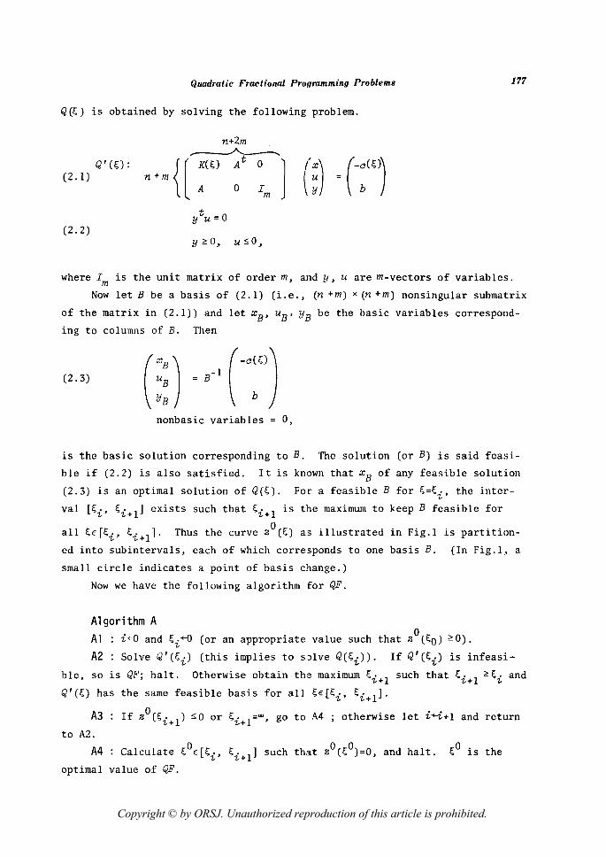
Q(S) is obtained by solving the following problem.

Q'(S) : (2.1)

/u=O (2.2)

Y"C:O, u~O,

where I is the unit matrix of order m, and y, u are m-vectors of variables. m Now let B be a basis of (2.1) (Le., (n +m) x (n +m) nonsingular submatrix

of the matrix in (2.1)) and let xB' uB' YB be the basic variables correspond

ing to columns of B. Then

(2.3)

nonbasic variables 0,

is the basic solution corresponding to B. The solution (or B) is said feasi

ble if (2.2) is also satisfied. It is known that xB of any feasible solution

(2.3) is an optimal solution of Q(S). For a feasible B for s=si' the inter

val [si' si+l] exists such that Si+l is the maximum to keep B feasible for

° all SE [si' si+ 1] . Thus the curve z (S) as illustrated in Fig.l is parti tion-

ed into subintervals, each of which corresponds to one basis B. (In Fig.l" a

small circle indicates a point of basis change.)

Now we have the following algorithm for QF.

Algorithm A Al i+O and si+O (or an appropriate value such that ZO(SO) "C:O).

A2 : Solve Q'(si) (this implies to solve Q(si))' If Q'(si) is infeasi

ble, so is QF; halt. Otherwise obtain the maximum si+l such that si+l "C:si and

Q'(s) has the same feasible basis for all SE[si' si+l]'

A3 otherwise let i+i+l and return

to A2.

A4 : Calculate SOE[Si' si+l] such that ZO(sO)=O, and halt. sO is the

optimal value of QF.


178 T. lbaraki, H. lahii, J. IWQae, T. HaaegaWQ and H. Mine

Remark 2. 1. Q'(~i) is solved in finite steps for example by the Wolfe's

method [5,2]: (The Wolfe's method is used in the experiment of Section 6.)

Given an optimal tableau for Q'(~i)' an optimal tableau for Q'(~i+l) is easily

obtained by using the parametric programming technique developed by Ritter [4]

and Wolfe [5] (Wolfe treats the case of D=O) in one pivot operation (provided

that the nondegeneracy assumption holds). It is not necessary to solve Q'(

~i+l) from the initial tableau.

Remark 2.2. ~i+l in Step A2 is obtained from (2.3) by calculating the

maximum of ~'(~~i) such that the basic feasible solution (2.3) is feasible for

all ~ satisfying ~i~~~~" (See Example 3.1 of Section 3, in which this pro

cess is carried out.) If D=O, this computation becomes particularly simple

(as studied by Wolfe [5]) since B- 1 is independent of~. (D=O is assumed in

the computational experiment in Section 6.)

Remark 2.3. ~O in Step A4 is the solution of equation

(2.4)

which is the smallest not smaller than ~i' where x is given by (2.3). If D=O,

(2.4) is a quadratic equation, and the smaller of two solutions is ~O. Remark 2.4. An optimal solution of QF is easily obtained from (2.3) by

setting ~=~O.

3. Finiteness of Algorithm A

Provided that a finite algorithm is used to solve Q'(~i) in Step A2 (see

Remark 2.1), Algorithm A is proved to be finite if the number of intervals of

zO(~) each of which corresponds to a basis (see Section 2) is finite. Since

the number of possible bases of (2.1) is finite, it then suffices to show that

the same basis B appears only finitely many times corresponding to different

intervals.

Note that the finiteness is not tirvial since there is a case in which

the same basis corresponds to more than one interval, as given in the next

example. It also helps to visualize the idea used in the proof for the fi

niteness in the latter half of this section.

Example 3.1.


Quadratic Fractional Programming Problem8 179

QF maximize

[ -: :: ] (:: ) + (1, -1) (::) + 180

: J ( :: ) + (-1,-7) + 1

subject to

The objective function of Q(~) is then given by

Constraint (2.1) of the Kuhn-Tucker theorem is

-1-~ -1 1 -1 0 xl

0 x 2 1 -2-~ 1 0 -1

1 1 ~1 7

-1 0 0 I3 u

3 0

0 -1 Y1 0 : Y 3

Now take the following basis

-1-~ -1 o 1 -2-~

(3.1) B = 1 1

-1 0

0 -1


180 T. Ibaraki, H. Ishii, J. lwase, T. Hahegawa and H. Mine

8- 1 is then

where

given by

(-2-~)/t. 1 It.

-1 It. ( -1-~)/t.

B- 1 (3 +~)/t. ~ It.

(-2-Q/t. 1 It.

-1 It. ( -1-~)/t.

2 t. = det B = 3 + 3~ + ~ •

(] (3-4~ +~ 2) Ill.

(n+n2

)/ll.

(l8+18~-~2)/t.

(3_4~+~2)/ll.

(7~+n2)/ll.

Since ll.>O for any ~, and

Y1 ~ 0 for -0.95 ~E; ~ 18.95

Y2 ~o for ~ 51 or ~ ~ 3

Y3 ~o for ~ ~ 1 or ~ ~ 0,

(2.2) is satisfied in two intervals :

[-0.95, 1) and [3, 18.95).

o

When Algorithm A starts from ~O=O, therefore, basis B of (3.1) appears

twice corresponding to intervals

[0, 1) and [3, 18.95].

It was first proved by Ritter [4] in a more general setting that a basis


Quadratic Fractional Pro.qmmming Problems

B appears only finitely many times as feasible basis when ~ is continuously

increased.

181

In the following, the same result is proved by deriving an explicit upper

bound (not given in [4]) on how many times a basis B appears in Step A2, by

refining the argument used in Sections 3 and 4 of [4].

It is known in the theory of quadratic programming (e.g., [4]) that con

dition ytu=O of (2.2) permits us to consider only a basic solution with basis

of the form

(3.2) B

n k m-k ......, At

1

o

o

} n

} k

} m-k,

where A =[~~J ' and (kxn) matrix Al has full rank. Thus we consider in the

subsequent discussion only bases in this form. Since K(~) is assumed to be

negative definite,

(3.3)

holds for any ~.

Lemma 3.1. B of (3.2) satisfies

for any~. (Thus det B does not change its sign when ~ is continuously in

creased.)

Proof. n n [ K(f.)

( -1) det B = (-1) det Al (by (3.2))

n -1 t =(-1) det K(~) det [-AIK(~) Al J>O.


182 T. lbaraki, H. Ishii, J. Iwase, T. Hasegawa and H. Mine

The last relation follows from (3.3) and the property that - AlK(;) -1 Alt is

-1 t positive definite (hence det [- ~K(~) '\] > 0). Q.E.D.

Lemma 3.2. Let ui and Y j be elements of uB and YB defined in (2.3) for B

of (3.2). Then the number of intervals in which ui assumes nonpositive values

when ~ is changed from 0 to 00 is at most r n-~+21 ' wher~ r xl denotes the

smallest integer not smaller than x. Similarly, the number of intervals in

. rn-k+ll which Yj assumes nonnegative values 1S at most ---2--- •

Proof. From (2.3), we have

•• -1 (-e~<J)

(3.4)

fl2l

/t:. ..• tn-tm~/fl ] (-a~~)) • . . . . • . tn-tmn-tm/ t:.

where t:.ij is the (i, j)-th cofactor of Band t:.= det B. Since each element of

K(~) is linear in ~ and other elements of B do not depend on ~, the degree (in

~) of the numerator of each element of B- 1 is easily calculated ; it is given

below.

k m-k

(n-k-l) 1

(n-k) } I (0) n 1 I ---------,------------------I I

I } k (3.5) (n-k) I (n-k+l) I (0) 1 I

- - - - - - - - -1- - - - - - - - - - - - - - - - - --

(n-k-l) 1

(n-k) 1 1

(0) } m-k

Note that only the numerator is important from the view point of the sign, since

the denominator t:. does not change its sign by Lemma 3.1. From (3.5), the de

grees of the numerators of xB' uB' YB are obtained, using that a(~) is linear

in ~ :

(3.6) ( _~~=~~_) } n (n-k+l) } k -------

(n-k) } m-k.


Quadratic Fractional Programming Problems 183

Now note that the number of intervals in which a polynomial of degree r as-

. ( . .) . r r+11 sumes nonnegat1ve nonpos1 t1ve values 1S at most -2- . By (3.6), this

proves the lemma statement. Q.E.D.

Theorem 3.3. Let B be given by (3.2). When ~ is increased from 0 to 00,

the number of intervals of ~ in which uB and YB of basic solution (2.3) satis

fy uBsO and YB~O (i.e., feasible) is at most

(3.7)

Proof. Let Pi(~) be a polynomial of degree ri' i=I,2, ... ,m. Then it is

easy to show that the number of intervals of ~ in which PI (~), ... , Pk(~) are

nonpositive and Pk+1 (~), ... , Pm(~) are nonnegative is at most

(3.8) ..m r r .+1 1 Li=l -T- - (m-I).

(3.7) follows from (3.8) by substituting

{

n-k+l

n-k

obtained in Lemma 3.2.

Corollary 3.4. N(n) = 1.

i=1,2, ... , k

i=k+1, ... , m

Q.E.D.

A basis B with k=n represents an extreme point of polyhedron Axsb. This

corollary tells that such basis appears at most once as a feasible basis in

Algorithm A.

Corollary 3.5. N(O) =mr n;l 1 + I-m.

Note that a basis B with k=O corresponds to an interior point of poly

hedron A:csb.

Theorem 3.6. Algorithm A of Section 2 gives an optimal solution of QF


184 T. lbaraki, H. Ishii, J. l!Case, T. Ha.~egawa and H. Mine

or indicates its infeasibility, after executing Step A2 finite times, provided

that Q' (~.l· is solved by a finite algorithm. 'l-

Proof. The finiteness follows from the argument given in the beginning

of this section and Theorem 3.3. If Algorithm A halts in Step A2 indicating

the infeasibility of Q' (~i)' then Ax~b is vacuous (i.e., QF is infeasible)

since it is known that a quadratic programming problem with a negative defi

nite objective function (such as Q(~i)) always has an optimal solution ifAx~b

is not vacuous. On the other hand, if Algorithm A halts in Step A4, ~o is the

maximum value of QF as proved in [1,3]. Q.E.D.

4. Two special cases

In this section, two special cases D=O and C=O are discussed. In either

case, it is shown that each basis B appears at most once in Algorithm A.

Theorem 4.1. Assume D=O in QF. Then a basis B of (3.2) appears at most

once as a feasible basis of Q' (~) in Step A2 of Algorithm A.

Proof. In this case, no element of B of (3.2) contains ~ since K(~)=C-~D

=C ; hence no element of B- 1 contains~. Thus xB' uB' YB given by (2.3) is

linear in variable ~, since -c(~) is linear in~. Letting Pi=1 in (3.8) gives

N(k)=l in the proof of Theorem 3.3. Q.E.D.

As mentioned in remarks given to Algorithm A, the case of D=O has also

other computational advantages. The computational experiment in Section 6 is

therefore done for this simple case only.

The case of C=Q is similar. However, it is necessary to assume that

(4.1) D is positive definite

(4.2) t P x+s > ° for some XES

in addition to (1.4), since C is not negative definite in this case. Algo

rithm A should be started from ~Q=o, where 0 is an appropriate positive number

satisfying zO(o) ~o.

Theorem 4.2. Assume C=Q in QF and let (4.1) (4.2) be satisfied. Then

basis B of (3.2) appears at most once as a feasible basis in Step A2 of Algo

rithm A, provided that ~O is set to the above 0 in Step Al.


Quadratic Fractional Progmmming Problem.~

Proof. In this case, B of (3.2) is given by

-t:D A t 1

0

B Al 0 0

A2 0 I m-k

In a manner similar to the proof of Lemma 3.1, we have

-1 t fI(=detB)=detK(t:) det [-AI KW AI]

-1 Thus B in this case has the following form.

n

1 -a F,

a

I 1 I - a I t: I

k r-.

a

t:a

a

m-k r-.

a } n

a } k

a } m-k

where a stands for a real number independent of t: (each a may represents a

different number). Since it can be written that

} n

} m

by using the same notation as above, we have

-c (t:) 1 } -(t:a+B) n t:

--------

=B -1

t:a+8 } k

--------

b 1 ~(t:a+8) } m-k

This proves that the numerator of each element of xB' uB ' YB is linear in (,

185


186 T. Ibaraki, H. Ishii, J. Iwase, T. Hasegawa and H. Mine

the denominator does not change its sign by Lemma 3.1 and E;>O. Thus we can

let r.=l iri (3.8), obtaining N(k)=l in the proof of Theorem 3.3. Q.E.O. "1.-

5. Dinkelbach's method and its modification

In order to solve QF, the Oinke1bach's method [1] may also be directly

applied. It obtains E;* (~O) and the corresponding feasible solution x* of QF

such that

where £ is a given nonnegative constant.

Dinkelbach's algorithm

Dl : i+O, E;i+O (or an appropriate value such that BO(E;o)~O). D2 : Solve Q'(E;i)' If Q' (E;i) is infeasible, so is QF ; halt. Otherwise

let x-part of a feasible solution of Q' (E;i) be xCi) (i.e., xCi) is an optimal

solution of Q(~i))'

D3 : If BO(~i)$£, let ~*+~i' x*+x(i) and halt; otherwise

1 . tc. . t. 1· tv. . t . E;i+l + (Z X ("1.-) x("1.-)+r X("1.-)+8)/(Z x("1.-) :x:("1.-)+P X("1.-)+q)

i +i+l

and return to 02.

If £>0, this algorithm halts after executing Steps D2 and D3 finitely

many times. If £=0, i.e., an exact optimal solution is sought, however, this

a.lgorithm usually requires an infinite number of iterations of Steps 02 and

03. This difficulty can be easily removed by modifying it as follows, by mak

ing use of the property that interval [~i' ~i'] maintaining the same basis is

easily calculated as discussed in Section 2. (This idea is also implicitly

used in the numerical example in Appendix of [1].)

Algorithm B (Modified Oinkelbach's method)

Bl : i+o, E;i+O (or an appropriate value such that ZO(~O)~O). B2 : Solve Q' (~i)' If Q' (~i) is infeasible, so is QF ; halt. Otherwise

obtain the maximum ~i' such that E;i' ~~i and Q' (~) has the same feasible basis

for all ~e: [~i' ~i']' Let x-part of a feasible solution of Q' (E;i' ) be x' (i)


Quadratic Fractional Progmmming Problems

(i.e., x' (i) is an optimal solution of Q' (E;i' )). o 83 If z (E;.' )$0 or E;.' =00, go to B4 ; otherwise

'/- '/-

1 . t . t . / 1 . t .) t .) E;i+l +- (2 x' ('/-) ex' ('/-)+1' x' ('/-)+8) (2 x' ('/-) Dx' ('/- +p x' ('/- +q)

i +- i+ 1

and return to B2.

187

o 0 0 84: Calculate E; E[E;., E;.'] such that z (E; )=0 and halt '/- '/-

E;0 is the maxi-

mum value of QF.

The computational process of these algorithms are illustrated in Fig.2,

in which solid arrows correspond to Algorithm B and broken arrows to the

Dinkelbach's method. E;i generated in the Dinkelbach's method is shown with

bar ~i to distingush it from E;i of Algorithm B. It is noted that E;i+l obtain

ed in Step D3 (resp. Step B3) is given as the intersection point of E;-axis and

the line tangent to zO (E;) at ~i (resp. E;i'). From Fig.2, it may be seen that

Algorithm B requires less number of iterations than the original Dinkelbach's

method.

Fig. 2. Illustration of computational processes of the

Dinkelbach's method and Algorithm B. (Solid arrows

indicate Algorithm B and broken arrows indicate the

Dinkelbach's method.)


188 T. lbaraki. H. Ishii. J. Iwase. T. Hasegawa and H. Mine

Remark 5.1. Q' (~.) (i>O) in Steps 02 or B2 may be solved starting from . 1.-

the final t~bleau of Q' (F,. 1)' This is a great computational saving, compared 1.--

with solving Q' (~.) from scratch. However, it may still require a considera-1.-

ble number of pivot operations if ~i is far from ~i-l' This should be compar-

ed with the fact that only one pivot operation is required in Algorithm A to

solve Q' (~.) (Remark 2.1). Although Step B2 of Algorithm B is usually carried 1.-

out far fewer times than Step A2 of Algorithm A, it is not clear which of

Algori thm A and Algorithm B is more efficient.

Theorem 5.1. Algorithm B gives an optimal solution of QF or indicates

its infeasibility, after executing Step B2 finite times, provided that Q' (~i)

is solved by a finite algorithm.

Proof. The validity of Algorithm B follows from the validity of the

Dinkelbach's method [1]. The finiteness can be proved in a manner similar to

Algorithm A (Theorem 3.6). Q.E.D.

6. Computational results

Algorithm A and Algorithm B discussed in the previous sections are imple

mented in FORTRAN and run on FACOM 230/60 (roughly equivalent to IBM 360/65 or

UNIVAC 1108) and FACOM 230/75 (roughly equivalent to IBM 370/165) of Kyoto

University. Problems QF with D=O (see (1.3)) are exclusively treated in the

experiment.

For various sizes n and m of QF, coefficients are randomly generated by

the following rule :

C : A negative definite symmetric matrix C of size nxn is obtained by

C =_ppt

for a nonsingular matrix P. P is generated by (i) randomly specifying non zero

elements of P with probability NZC (program parameter), (ii) assigning a non

negative (two digit) number randomly taken from the uniform distribution with

interval [0.0, 9.9] to each non zero element, and (iii) randomly inverting the

sign of nonzero elements with probability NC (program parameter). Note that

C has a considerably higher non zero density than NZC ; for example, C of two

typical problems in Table 1 have nonzero densities 89.5% for NZC=0.4 and 56%

for NZC=O. 25.


Quadratic Fractional Pro.qrammin.q Problems 189

A : An mXn matrix A is generated by (i) randomly specifying non zero ele

ments with probability NZA (program parameter), (ii) assigning a nonnegative

(three digit) number randomly taken from interval [00.0, 99.9] to each nonzero

element, and (iii) randomly inverting the sign of nonzero elements with proba

bility NA (program parameter).

1', p : Each element is assigned a (h'o digit) nonnegative number randomly

taken from [0.0, 9.9].

b : Each element is assigned a (four digit) positive number randomly

taken from [100.0, 199.9].

8=20.0 and q=3.0 for all problems.

Tables 1 and 2 summarize the computational results. The results in Table

1 are the average of 10 problems with n=m=20, while Table 2 lists results for

each problem of larger size.

Table 1. Computational results for problems with n=20 and m=20.

(All figures are the average of 10 problems.)

Q' (f;0) Q' (f;i), i>O Total

Algorithm Iteration time

Pivot(a) Time(c) Pivot (b) Time(c) (e) (sec. )

(sec. ) (sec. ) (c, f)

A 114.7 12.7 14.1 1.9 15.1 14.6

B 114.7 12.7 19.9 2.9 2.6 15.6

Remark

NZA=OA-

NZC=0.2-

NA=0.2-

NC=0.2-

O. 7

0.5

0.4

0.4


190 T. Ibaraki. H. Ishii, J. Iwase, T. Hasegawa and H. Mine

Table 2. Computational results for large problems

Q'(~O) Q' (~.), i>o Itera- Total 1.-

Problem Algorithm tion Time Remark Pivot Time (d) Pivot Time (d)

(e) (sec. ) (a) (sec. ) (b) (sec. ) (d, f)

n=40 A 344 31. 8 25 2.7 25 34.5 NZA=0.6 NZC=0.4 m=40 B 344 31.8 22 2.5 2 34.3 NA=NC=0.2

n=50 A 586 85.3 25 4.2 26 89.5 NZA=0.7 NZC=0.4 m=50 B 586 85.3 53 9.6 2 94.9 NA=NC=0.2

n=50 A 606 83.2 27 4.5 28 87.7 NZA=0.5 NZC=0.4 m=50 B 606 83.2 68 12.5 2 95.7 NA=NC=0.2

n=50 A 575 71.1 24 3.9 25 75.0 NZA=0.35

m=50 B 575 71.1 39 6.7 2 77 .8 NZC=0.4 NA=NC=0.2

n=50 A 694 110.6 29 4.8 30 115.4 NZA=0.4

m=50 B 694 110.6 57 9.5 3 120.1 NZC=0.17 NA=NC=0.2

Notes (a) The number of pivots required to solve Q'(~O) by the Wolfe's method.

(b) The number of pivots required to solve Q' (~i) for all i>O.

(c) Machine is PACOM 230/60.

(d) Machine is PACOM 230/75.

(e) The number of executions of A2 (or B2) including the ones for Q'(~O)'

(f) Including the computation for A3, A4 (or B3, B4).

From these results, it may be concluded that Algorithm A is slightly

faster than Algorithm B but there is no significant difference. It is also

noticed that computation for Q' (~O) (the first one) in Step A2 or B2 is rather

expensive compared with the rest (Le., computation for Q' (~.), i>O) com-1.-


Quadratic Fractional Pro.qramming Problems 191

putation for Q' (E;O) consumes roughly 80~90't of the entire computation time.

Thus the use of parametric programming technique seems quite effective. This

also explains a reason for the similarity (in computation time) of Algorithm A

and Algorithm B mentioned above ; two algorithms differ only in the way of

generating E;i for i>O.

It is also observed that program parameters specifying the ratios of non

zero and negative coefficients do not have much influence on the relative be

havior of Algorithms A and B, though the higher values tend to increase the

computation time. Table 1 includes problems with various parameter values.

In conclusion, it can be said that the quadratic fractional programming

problem with D=O is a rather easy nonlinear programming problem, which can be

solved in computational effort only slightly greater than that required for

the well known (concave) quadratic programming problem.

Acknowledgement The authors are indebted to Miss T. Kanazawa for her excellent typing.

References [1] W. Dinkelbach, On nonlinear fractional programming, Management Science,

13 (1967), pp. 492-498.

[2] G. Hadley, Nonlinear and Dynamic Programming, Addison Wesley, 1964.

[3] R. Jagannathan, On some properties of programming problems in para

metric form pertaining to fractional programming, Management Science,

12 (1966), pp. 609-615.

[4] K. Ritter, Ein Verfahren zur Losung parameterabhangiger, nichitlinearer

Maximum-Probleme, Unternehmensforschung, 6 (1962), pp. 149-166.

(English translation by M. Meyer, A method for solving nonlinear maxi

mum-problems depending on parameters, Naval Research Logistics Quarter

ly, 14 (1967), pp. 147-162.)

[5] P. Wolfe, The simplex method for quadratic programming, Econometrica,

27 (1959), pp. 382-398.

(The authors' address: Department of Applied Mathematics and Physics, Faculty

of Engineering, Kyoto University, Kyoto Japan.)


algorithms for quadratic fractional programming problems

Documents

Transcript of algorithms for quadratic fractional programming problems