Algorithms and Ordering Heuristics for Distributed ...
161
HAL Id: tel-00718537 https://tel.archives-ouvertes.fr/tel-00718537v1 Submitted on 17 Jul 2012 (v1), last revised 27 Aug 2012 (v2) HAL is a multi-disciplinary open access archive for the deposit and dissemination of sci- entific research documents, whether they are pub- lished or not. The documents may come from teaching and research institutions in France or abroad, or from public or private research centers. L’archive ouverte pluridisciplinaire HAL, est destinée au dépôt et à la diffusion de documents scientifiques de niveau recherche, publiés ou non, émanant des établissements d’enseignement et de recherche français ou étrangers, des laboratoires publics ou privés. Algorithms and Ordering Heuristics for Distributed Constraint Satisfaction Problems Mohamed Wahbi To cite this version: Mohamed Wahbi. Algorithms and Ordering Heuristics for Distributed Constraint Satisfaction Prob- lems. Artificial Intelligence [cs.AI]. Université Montpellier II - Sciences et Techniques du Languedoc; Université Mohammed V-Agdal, Rabat, 2012. English. tel-00718537v1
Transcript of Algorithms and Ordering Heuristics for Distributed ...

HAL Id: tel-00718537https://tel.archives-ouvertes.fr/tel-00718537v1
Submitted on 17 Jul 2012 (v1), last revised 27 Aug 2012 (v2)
HAL is a multi-disciplinary open accessarchive for the deposit and dissemination of sci-entific research documents, whether they are pub-lished or not. The documents may come fromteaching and research institutions in France orabroad, or from public or private research centers.
L’archive ouverte pluridisciplinaire HAL, estdestinée au dépôt et à la diffusion de documentsscientifiques de niveau recherche, publiés ou non,émanant des établissements d’enseignement et derecherche français ou étrangers, des laboratoirespublics ou privés.
Algorithms and Ordering Heuristics for DistributedConstraint Satisfaction Problems
Mohamed Wahbi
To cite this version:Mohamed Wahbi. Algorithms and Ordering Heuristics for Distributed Constraint Satisfaction Prob-lems. Artificial Intelligence [cs.AI]. Université Montpellier II - Sciences et Techniques du Languedoc;Université Mohammed V-Agdal, Rabat, 2012. English. �tel-00718537v1�

LIRMM
Université Montpellier 2 Université Mohammed V - AgdalSciences et Techniques du Languedoc Faculté des Sciences du RabatFrance Maroc
Ph.D Thesis
présentée pour obtenir le diplôme de Doctorat en Informatiquede l’Université Montpellier 2 & l’Université Mohammed V-Agdal
par
Mohamed Wahbi
Spécialité : Informatique
École Doctorale Information, Structures, Systèmes- France &Le Centre d’Etudes Doctorales en Sciences et Technologies de Rabat- Maroc
Algorithms and Ordering Heuristics forDistributed Constraint Satisfaction Problems
Soutenue le 03 Juillet 2012, devant le jury composé de :
President
Mme. Awatef Sayah, PES . . . . . . . . . . . . . . . . . . . . . . . . Université Mohammed V-Agdal, Maroc
Reviewers
Mr. Pedro Meseguer, Directeur de recherche . . . . . . . . . . . . . . . . . . . . IIIA, Barcelona, EspagneMr. Mustapha Belaissaoui, Professeur Habilité . . . . . l’ENCG, Université Hassan I, Maroc
Examinator
Mr. Rémi Coletta, Maitre de conférence . . . . . . . LIRMM, Université Montpellier 2, France
Supervisors
Mr. Christian Bessiere, Directeur de recherche . LIRMM, Université Montpellier 2, FranceMr. El Houssine Bouyakhf, PES. . . . . . . . . . . . . . . . . . Université Mohammed V-Agdal, Maroc


iii
To my family

Acknowledgements
The research work presented in this thesis has been performed in the Laboratoire
d’Informatique Mathématiques appliquées Intelligence Artificielle et Reconnaissance de
Formes (LIMIARF), Faculty of Science, University Mohammed V-Agdal, Rabat, Morocco
and the Laboratoire d’Informatique, de Robotique et de Microélectronique de Montpellier
(LIRMM), University Montpellier 2, France.
This thesis has been done in collaboration between University Mohammed V-Agdal,
Morocco and University Montpellier 2, France under the financial support of the scholar-
ship of the programme Averroés funded by the European Commission within the frame-
work of Erasmus Mundus.
First and foremost, it is with immense gratitude that I acknowledge all the support,
advice, and guidance of my supervisors, Professor El-Houssine Bouyakhf and Dr. Christian
Bessiere. It was a real pleasure to work with them. Their truly scientist intuition has
made them as a source of ideas and passions in science, which exceptionally inspire and
enrich my growth as a student, a researcher and a scientist want to be. I want to thank
them especially for letting me wide autonomy while providing appropriate advice. I am
indebted to them more than they know and hope to keep up our collaboration in the future.
I gratefully acknowledge Professor Awatef Sayah (Faculty of sciences, University Mo-
hammed V-Agdal, Morocco) for accepting to preside the jury of my dissertation. I am most
grateful to my reviewers Professor Pedro Meseguer (Scientific Researcher, the Artificial In-
telligence Research Institute (IIIA), Barcelona, Spain) and Professor Mustapha Belaissaoui
(Professeur Habilité, ENCG, University Hassan I, Morocco) for their constructive comments
on this thesis. I am thankful that in the midst of all their activities, they accepted to re-
view my thesis. I would like to record my gratitude to Professor Rémi Coletta, (Maître de
conférence, University Montpellier 2, France) for his thorough examination of the thesis.
Many of the works published during this thesis have been done in collaboration with so
highly motivated, smart, enthusiastic, and passionate coauthors. I want to thank them for
their teamwork, talent, hard work and devotion. I cannot thank my coauthors without giv-
ing my special gratefulness to Professor Redouane Ezzahir and Doctor Younes Mechqrane.
I thank the great staffs of the LIRMM and LIMIARF Laboratories for the use of facilities,
consultations and moral support. The LIRMM has provided the support and equipment
I have needed to produce and complete my thesis. I also want to thank my colleagues at
the LIRMM and LIMIARF Laboratories for the joyful and pleasant working environment.
v

vi Acknowledgements
Especially, I would like to thank the members of the Coconut/LIRMM and IA/LIMIARF
teams. I acknowledge Amine B., Fabien, Eric, Imade, Saida, Fred, Philippe, Brahim and
Jaouad.
In my daily work I have been blessed with a friendly and cheerful group of fellow
students. I would like to particularly thank Hajer, Younes, Mohamed, Kamel, Nawfal,
Mohammed, Nabil Z., Farid, Azhar, Kaouthar, Samir, Nabil Kh., Amine M., and Hassan.
It is a pleasure to express my gratitude wholeheartedly to Baslam’s family for their kind
hospitality during my stay in Montpellier.
Further, I am also very thankful to the professors of the department of Computer Sci-
ence, University Montpellier 2, with whom I have been involved as a temporary assistant
professor (Attaché Temporaire d’Enseignement et de Recherche - ATER) for providing an
excellent environment to teach and develop new pedagogical techniques. I convey special
acknowledgment to Professor Marianne Huchard.
Most importantly, words alone cannot express the thanks I owe to my family for be-
lieving and loving me, especially my mother who has always filled my life with generous
love, and unconditional support and prayers. My thanks go also to my lovely sister and
brother, my uncles and antes and all my family for their endless moral support throughout
my career. To them I dedicate this thesis. Last but not the least, the one above all of us, the
omnipresent God, for answering my prayers for giving me the strength to plod on despite
my constitution wanting to give up and throw in the towel, thank you so much Dear Lord.
Finally, I would like to thank everybody who was important to the successful realization
of thesis, as well as expressing my apology that I could not mention personally one by one.
Montpellier, July 3rd, 2012 Mohamed Wahbi

Abstract
Distributed Constraint Satisfaction Problems (DisCSP) is a general framework for solv-
ing distributed problems. DisCSP have a wide range of applications in multi-agent coor-
dination. In this thesis, we extend the state of the art in solving the DisCSPs by proposing
several algorithms. Firstly, we propose the Nogood-Based Asynchronous Forward Check-
ing (AFC-ng), an algorithm based on Asynchronous Forward Checking (AFC). However,
instead of using the shortest inconsistent partial assignments, AFC-ng uses nogoods as
justifications of value removals. Unlike AFC, AFC-ng allows concurrent backtracks to be
performed at the same time coming from different agents having an empty domain to
different destinations. Then, we propose the Asynchronous Forward-Checking Tree (AFC-
tree). In AFC-tree, agents are prioritized according to a pseudo-tree arrangement of the
constraint graph. Using this priority ordering, AFC-tree performs multiple AFC-ng pro-
cesses on the paths from the root to the leaves of the pseudo-tree. Next, we propose to
maintain arc consistency asynchronously on the future agents instead of only maintaining
forward checking. Two new synchronous search algorithms that maintain arc consistency
asynchronously (MACA) are presented. After that, we developed the Agile Asynchronous
Backtracking (Agile-ABT), an asynchronous dynamic ordering algorithm that does not fol-
low the standard restrictions in asynchronous backtracking algorithms. The order of agents
appearing before the agent receiving a backtrack message can be changed with a great free-
dom while ensuring polynomial space complexity. Next, we present a corrigendum of the
protocol designed for establishing the priority between orders in the asynchronous back-
tracking algorithm with dynamic ordering using retroactive heuristics (ABT_DO-Retro).
Finally, the new version of the DisChoco open-source platform for solving distributed con-
straint reasoning problems is described. The new version is a complete redesign of the
DisChoco platform. DisChoco 2.0 is an open source Java library which aims at implement-
ing distributed constraint reasoning algorithms.
Keywords: Distributed Artificial Intelligence, Distributed Constraint Satisfaction (DisCSP),
Distributed Solving, Maintaining Arc Consistency, Reordering, DisChoco.
vii


Résumé
Les problèmes de satisfaction de contraintes distribués (DisCSP) permettent de formali-
ser divers problèmes qui se situent dans l’intelligence artificielle distribuée. Ces problèmes
consistent à trouver une combinaison cohérente des actions de plusieurs agents. Durant
cette thèse nous avons apporté plusieurs contributions dans le cadre des DisCSPs. Pre-
mièrement, nous avons proposé le Nogood-Based Asynchronous Forward-Checking (AFC-
ng). Dans AFC-ng, les agents utilisent les nogoods pour justifier chaque suppression d’une
valeur du domaine de chaque variable. Outre l’utilisation des nogoods, plusieurs back-
tracks simultanés venant de différents agents vers différentes destinations sont autorisés.
En deuxième lieu, nous exploitons les caractéristiques intrinsèques du réseau de contraintes
pour exécuter plusieurs processus de recherche AFC-ng d’une manière asynchrone à tra-
vers chaque branche du pseudo-arborescence obtenu à partir du graphe de contraintes
dans l’algorithme Asynchronous Forward-Checking Tree (AFC-tree). Puis, nous proposons
deux nouveaux algorithmes de recherche synchrones basés sur le même mécanisme que
notre AFC-ng. Cependant, au lieu de maintenir le forward checking sur les agents non
encore instanciés, nous proposons de maintenir la consistance d’arc. Ensuite, nous propo-
sons Agile Asynchronous Backtracking (Agile-ABT), un algorithme de changement d’ordre
asynchrone qui s’affranchit des restrictions habituelles des algorithmes de backtracking
asynchrone. Puis, nous avons proposé une nouvelle méthode correcte pour comparer les
ordres dans ABT_DO-Retro. Cette méthode détermine l’ordre le plus pertinent en compa-
rant les indices des agents dès que les compteurs d’une position donnée dans le timestamp
sont égaux. Finalement, nous présentons une nouvelle version entièrement restructurée de
la plateforme DisChoco pour résoudre les problèmes de satisfaction et d’optimisation de
contraintes distribués.
Mots clefs : L’intelligence artificielle distribuée, les problèmes de satisfaction de contraintes dis-
tribués (DisCSP), la résolution distribuée, la maintenance de la consistance d’arc, les heuristiques
ordonnancement, DisChoco.
ix


Contents
Acknowledgements v
Abstract (English/Français) vii
Contents xi
Introduction 1
1 Background 7
1.1 Centralized Constraint Satisfaction Problems (CSP) . . . . . . . . . . . . . . . 7
1.1.1 Preliminaries . . . . . . . . . . . . . . . . . . . . . . . . . . . . . . . . . 9
1.1.2 Examples of CSPs . . . . . . . . . . . . . . . . . . . . . . . . . . . . . . 10
1.1.2.1 The n-queens problem . . . . . . . . . . . . . . . . . . . . . . 10
1.1.2.2 The Graph Coloring Problem . . . . . . . . . . . . . . . . . . 11
1.1.2.3 The Meeting Scheduling Problem . . . . . . . . . . . . . . . . 11
1.2 Algorithms and Techniques for Solving Centralized CSPs . . . . . . . . . . . 13
1.2.1 Algorithms for solving centralized CSPs . . . . . . . . . . . . . . . . . 14
1.2.1.1 Chronological Backtracking (BT) . . . . . . . . . . . . . . . . 15
1.2.1.2 Conflict-directed Backjumping (CBJ) . . . . . . . . . . . . . . 16
1.2.1.3 Dynamic Backtracking (DBT) . . . . . . . . . . . . . . . . . . 18
1.2.1.4 Partial Order Dynamic Backtracking (PODB) . . . . . . . . . 19
1.2.1.5 Forward Checking (FC) . . . . . . . . . . . . . . . . . . . . . . 20
1.2.1.6 Arc-consistency (AC) . . . . . . . . . . . . . . . . . . . . . . . 21
1.2.1.7 Maintaining Arc-Consistency (MAC) . . . . . . . . . . . . . . 23
1.2.2 Variable Ordering Heuristics for Centralized CSP . . . . . . . . . . . . 23
1.2.2.1 Static Variable Ordering Heuristics (SVO) . . . . . . . . . . . 24
1.2.2.2 Dynamic Variable Ordering Heuristics (DVO) . . . . . . . . . 25
1.3 Distributed constraint satisfaction problems (DisCSP) . . . . . . . . . . . . . . 28
1.3.1 Preliminaries . . . . . . . . . . . . . . . . . . . . . . . . . . . . . . . . . 29
1.3.2 Examples of DisCSPs . . . . . . . . . . . . . . . . . . . . . . . . . . . . 30
1.3.2.1 Distributed Meeting Scheduling Problem (DisMSP) . . . . . 31
1.3.2.2 Distributed Sensor Network Problem (SensorDCSP) . . . . . 32
1.4 Methods for solving distributed CSPs . . . . . . . . . . . . . . . . . . . . . . . 33
1.4.1 Synchronous search algorithms on DisCSPs . . . . . . . . . . . . . . . 34
1.4.1.1 Asynchronous Forward-Checking (AFC) . . . . . . . . . . . . 35
1.4.2 Asynchronous search algorithms on DisCSPs . . . . . . . . . . . . . . 37
xi

1.4.2.1 Asynchronous Backtracking (ABT) . . . . . . . . . . . . . . . 37
1.4.3 Dynamic Ordering Heuristics on DisCSPs . . . . . . . . . . . . . . . . 42
1.4.4 Maintaining Arc Consistency on DisCSPs . . . . . . . . . . . . . . . . . 43
1.5 Summary . . . . . . . . . . . . . . . . . . . . . . . . . . . . . . . . . . . . . . . . 43
2 Nogood based Asynchronous Forward Checking (AFC-ng) 45
2.1 Introduction . . . . . . . . . . . . . . . . . . . . . . . . . . . . . . . . . . . . . . 46
2.2 Nogood-based Asynchronous Forward Checking . . . . . . . . . . . . . . . . 47
2.2.1 Description of the algorithm . . . . . . . . . . . . . . . . . . . . . . . . 47
2.3 Correctness Proofs . . . . . . . . . . . . . . . . . . . . . . . . . . . . . . . . . . 51
2.4 Experimental Evaluation . . . . . . . . . . . . . . . . . . . . . . . . . . . . . . . 52
2.4.1 Uniform binary random DisCSPs . . . . . . . . . . . . . . . . . . . . . 52
2.4.2 Distributed Sensor Target Problems . . . . . . . . . . . . . . . . . . . . 55
2.4.3 Distributed Meeting Scheduling Problems . . . . . . . . . . . . . . . . 56
2.4.4 Discussion . . . . . . . . . . . . . . . . . . . . . . . . . . . . . . . . . . . 58
2.5 Other Related Works . . . . . . . . . . . . . . . . . . . . . . . . . . . . . . . . . 59
2.6 Summary . . . . . . . . . . . . . . . . . . . . . . . . . . . . . . . . . . . . . . . . 59
3 Asynchronous Forward Checking Tree (AFC-tree) 61
3.1 Introduction . . . . . . . . . . . . . . . . . . . . . . . . . . . . . . . . . . . . . . 62
3.2 Pseudo-tree ordering . . . . . . . . . . . . . . . . . . . . . . . . . . . . . . . . . 63
3.3 Distributed Depth-First Search trees construction . . . . . . . . . . . . . . . . 64
3.4 The AFC-tree algorithm . . . . . . . . . . . . . . . . . . . . . . . . . . . . . . . 67
3.4.1 Description of the algorithm . . . . . . . . . . . . . . . . . . . . . . . . 68
3.5 Correctness Proofs . . . . . . . . . . . . . . . . . . . . . . . . . . . . . . . . . . 70
3.6 Experimental Evaluation . . . . . . . . . . . . . . . . . . . . . . . . . . . . . . . 70
3.6.1 Uniform binary random DisCSPs . . . . . . . . . . . . . . . . . . . . . 71
3.6.2 Distributed Sensor Target Problems . . . . . . . . . . . . . . . . . . . . 73
3.6.3 Distributed Meeting Scheduling Problems . . . . . . . . . . . . . . . . 74
3.6.4 Discussion . . . . . . . . . . . . . . . . . . . . . . . . . . . . . . . . . . . 76
3.7 Other Related Works . . . . . . . . . . . . . . . . . . . . . . . . . . . . . . . . . 76
3.8 Summary . . . . . . . . . . . . . . . . . . . . . . . . . . . . . . . . . . . . . . . . 76
4 Maintaining Arc Consistency Asynchronously in Synchronous Distributed
Search 77
4.1 Introduction . . . . . . . . . . . . . . . . . . . . . . . . . . . . . . . . . . . . . . 78
4.2 Maintaining Arc Consistency . . . . . . . . . . . . . . . . . . . . . . . . . . . . 79
4.3 Maintaining Arc Consistency Asynchronously . . . . . . . . . . . . . . . . . . 79
4.3.1 Enforcing AC using del messages (MACA-del) . . . . . . . . . . . . . 80
4.3.2 Enforcing AC without additional kind of message (MACA-not) . . . . 83
4.4 Theoretical analysis . . . . . . . . . . . . . . . . . . . . . . . . . . . . . . . . . . 84
4.5 Experimental Results . . . . . . . . . . . . . . . . . . . . . . . . . . . . . . . . . 85
4.5.1 Discussion . . . . . . . . . . . . . . . . . . . . . . . . . . . . . . . . . . . 87
4.6 Summary . . . . . . . . . . . . . . . . . . . . . . . . . . . . . . . . . . . . . . . . 88
xii
5 Agile Asynchronous BackTracking (Agile-ABT) 89
5.1 Introduction . . . . . . . . . . . . . . . . . . . . . . . . . . . . . . . . . . . . . . 90
5.2 Introductory Material . . . . . . . . . . . . . . . . . . . . . . . . . . . . . . . . . 91
5.2.1 Reordering details . . . . . . . . . . . . . . . . . . . . . . . . . . . . . . 91
5.2.2 The Backtracking Target . . . . . . . . . . . . . . . . . . . . . . . . . . . 92
5.2.3 Decreasing termination values . . . . . . . . . . . . . . . . . . . . . . . 94
5.3 The Algorithm . . . . . . . . . . . . . . . . . . . . . . . . . . . . . . . . . . . . . 95
5.4 Correctness and complexity . . . . . . . . . . . . . . . . . . . . . . . . . . . . . 98
5.5 Experimental Results . . . . . . . . . . . . . . . . . . . . . . . . . . . . . . . . . 100
5.5.1 Uniform binary random DisCSPs . . . . . . . . . . . . . . . . . . . . . 101
5.5.2 Distributed Sensor Target Problems . . . . . . . . . . . . . . . . . . . . 103
5.5.3 Discussion . . . . . . . . . . . . . . . . . . . . . . . . . . . . . . . . . . . 104
5.6 Related Works . . . . . . . . . . . . . . . . . . . . . . . . . . . . . . . . . . . . . 106
5.7 Summary . . . . . . . . . . . . . . . . . . . . . . . . . . . . . . . . . . . . . . . . 106
6 Corrigendum to “Min-domain retroactive ordering for Asynchronous Backtrack-
ing” 107
6.1 Introduction . . . . . . . . . . . . . . . . . . . . . . . . . . . . . . . . . . . . . . 107
6.2 Background . . . . . . . . . . . . . . . . . . . . . . . . . . . . . . . . . . . . . . 108
6.3 ABT_DO-Retro May Not Terminate . . . . . . . . . . . . . . . . . . . . . . . . 110
6.4 The Right Way to Compare Orders . . . . . . . . . . . . . . . . . . . . . . . . . 112
6.5 Summary . . . . . . . . . . . . . . . . . . . . . . . . . . . . . . . . . . . . . . . . 114
7 DisChoco 2.0 115
7.1 Introduction . . . . . . . . . . . . . . . . . . . . . . . . . . . . . . . . . . . . . . 115
7.2 Architecture . . . . . . . . . . . . . . . . . . . . . . . . . . . . . . . . . . . . . . 116
7.2.1 Communication System . . . . . . . . . . . . . . . . . . . . . . . . . . . 117
7.2.2 Event Management . . . . . . . . . . . . . . . . . . . . . . . . . . . . . . 118
7.2.3 Observers in layers . . . . . . . . . . . . . . . . . . . . . . . . . . . . . . 118
7.3 Using DisChoco 2.0 . . . . . . . . . . . . . . . . . . . . . . . . . . . . . . . . . . 119
7.4 Experimentations . . . . . . . . . . . . . . . . . . . . . . . . . . . . . . . . . . . 121
7.5 Conclusion . . . . . . . . . . . . . . . . . . . . . . . . . . . . . . . . . . . . . . . 123
Conclusions and perspectives 125
Bibliography 129
List of Figures 139
List of Tables 141
List of algorithms 143
xiii


Introduction
Constraint programming is an area in computer science that has gained increasing
interest in the last four recent decades. Constraint programming is based on its powerful
framework named Constraint Satisfaction Problem (CSP). A constraint satisfaction problem is
a general framework that can formalize many real world combinatorial problems. Various
problems in artificial intelligence can be naturally modeled as CSPs. Therefore, the CSP
paradigm has been widely used for solving such problems. Examples of these problems
can inherent from various areas related to resource allocation, scheduling, logistics and
planning. Solving a constraint satisfaction problem (CSP) consists in looking for solutions
to a constraint network, that is, a set of assignments of values to variables that satisfy the
constraints of the problem. These constraints represent restrictions on values combinations
allowed for constrained variables.
Numerous powerful algorithms were designed for solving constraint satisfaction prob-
lems. Typical systematic search algorithms try to construct a solution to a CSP by incre-
mentally instantiating the variables of the problem. However, proving the existence of
solutions or finding these solutions in CSP are NP-complete tasks. Thus, many heuristics
were developed to improve the efficiency of search algorithms.
Sensor networks [Jung et al., 2001; Béjar et al., 2005], military unmanned aerial vehicles
teams [Jung et al., 2001], distributed scheduling problems [Wallace and Freuder, 2002;
Maheswaran et al., 2004], distributed resource allocation problems [Petcu and Faltings,
2004], log-based reconciliation [Chong and Hamadi, 2006], Distributed Vehicle Routing
Problems [Léauté and Faltings, 2011], etc. are real applications of a distributed nature, that
is, knowledge is distributed among several physical distributed entities. These applications
can be naturally modeled and solved by a CSP process once the knowledge about the whole
problem is delivered to a centralized solver. However, in such applications, gathering the
whole knowledge into a centralized solver is undesirable. In general, this restriction is
mainly due to privacy and/or security requirements: constraints or possible values may
be strategic information that should not be revealed to others agents that can be seen as
competitors. The cost or the inability of translating all information to a single format
may be another reason. In addition, a distributed system provides fault tolerance, which
means that if some agents disconnect, a solution might be available for the connected part.
Thereby, a distributed model allowing a decentralized solving process is more adequate.
The Distributed Constraint Satisfaction Problem (DisCSP) has such properties.
A distributed constraint satisfaction problem (DisCSP) is composed of a group of au-
tonomous agents, where each agent has control of some elements of information about
the whole problem, that is, variables and constraints. Each agent owns its local constraint
network. Variables in different agents are connected by constraints. In order to solve a
1
2 Introduction
DisCSP, agents must assign values to their variables so that all constraints are satisfied.
Hence, agents assign values to their variables, attempting to generate a locally consistent
assignment that is also consistent with constraints between agents [Yokoo et al., 1998;
Yokoo, 2000a]. To achieve this goal, agents check the value assignments to their variables
for local consistency and exchange messages among them to check consistency of their pro-
posed assignments against constraints that contain variables that belong to others agents.
In solving DisCSPs, agents exchange messages about the variable assignments and con-
flicts of constraints. Several distributed algorithms for solving DisCSPs have been designed
in the last two decades. They can be divided into two main groups: asynchronous and syn-
chronous algorithms. The first category are algorithms in which the agents assign values
to their variables in a synchronous, sequential way. The second category are algorithms
in which the process of proposing values to the variables and exchanging these proposals
is performed asynchronously between the agents. In the former category, agents do not
have to wait for decisions of others, whereas, in general only one agent has the privilege of
making a decision in the synchronous algorithms.
Contributions
A major motivation for research on distributed constraint satisfaction problem (DisCSP)
is that it is an elegant model for many every day combinatorial problems that are dis-
tributed by nature. By the way, DisCSP is a general framework for solving various problems
arising in Distributed Artificial Intelligence. Improving the efficiency of existing algorithms
for solving DisCSP is a central key for research on DisCSPs. In this thesis, we extend the
state of the art in solving the DisCSPs by proposing several algorithms. We believe that
these algorithms are significant as they improve the current state-of-the-art in terms of
runtime and number of exchanged messages experimentally.
Nogood-Based Asynchronous Forward Checking (AFC-ng) is an asynchronous algo-
rithm based on Asynchronous Forward Checking (AFC) for solving DisCSPs. In-
stead of using the shortest inconsistent partial assignments AFC-ng uses nogoods as
justifications of value removals. Unlike AFC, AFC-ng allows concurrent backtracks
to be performed at the same time coming from different agents having an empty
domain to different destinations. Thanks to the timestamps integrated in the CPAs,
the strongest CPA coming from the highest level in the agent ordering will eventually
dominate all others. Interestingly, the search process with the strongest CPA will
benefit from the computational effort done by the (killed) lower level processes. This
is done by taking advantage from nogoods recorded when processing these lower
level processes.
Asynchronous Forward-Checking Tree (AFC-tree) The main feature of the AFC-tree al-
gorithm is using different agents to search non-intersecting parts of the search space
concurrently. In AFC-tree, agents are prioritized according to a pseudo-tree arrange-
ment of the constraint graph. The pseudo-tree ordering is built in a preprocessing
step. Using this priority ordering, AFC-tree performs multiple AFC-ng processes on
the paths from the root to the leaves of the pseudo-tree. The agents that are brothers
Introduction 3
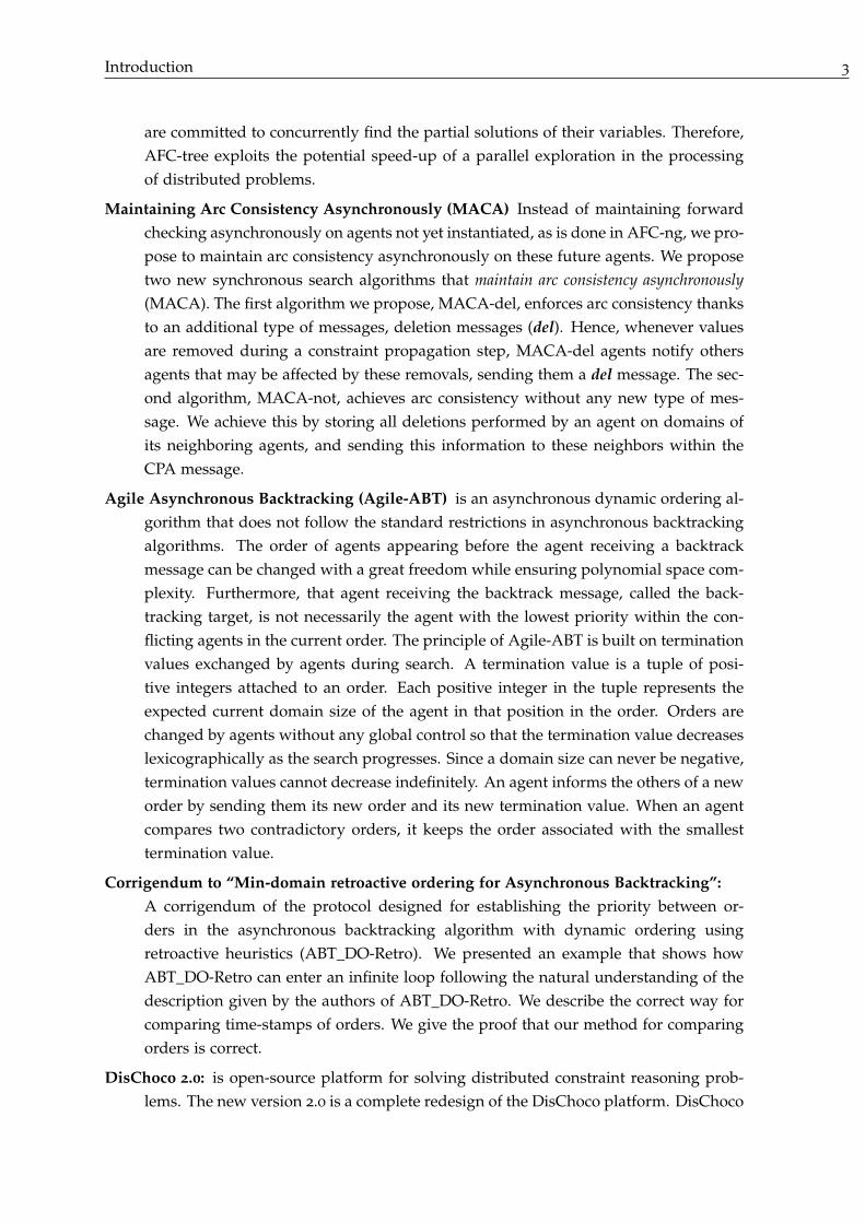
are committed to concurrently find the partial solutions of their variables. Therefore,
AFC-tree exploits the potential speed-up of a parallel exploration in the processing
of distributed problems.
Maintaining Arc Consistency Asynchronously (MACA) Instead of maintaining forward
checking asynchronously on agents not yet instantiated, as is done in AFC-ng, we pro-
pose to maintain arc consistency asynchronously on these future agents. We propose
two new synchronous search algorithms that maintain arc consistency asynchronously
(MACA). The first algorithm we propose, MACA-del, enforces arc consistency thanks
to an additional type of messages, deletion messages (del). Hence, whenever values
are removed during a constraint propagation step, MACA-del agents notify others
agents that may be affected by these removals, sending them a del message. The sec-
ond algorithm, MACA-not, achieves arc consistency without any new type of mes-
sage. We achieve this by storing all deletions performed by an agent on domains of
its neighboring agents, and sending this information to these neighbors within the
CPA message.
Agile Asynchronous Backtracking (Agile-ABT) is an asynchronous dynamic ordering al-
gorithm that does not follow the standard restrictions in asynchronous backtracking
algorithms. The order of agents appearing before the agent receiving a backtrack
message can be changed with a great freedom while ensuring polynomial space com-
plexity. Furthermore, that agent receiving the backtrack message, called the back-
tracking target, is not necessarily the agent with the lowest priority within the con-
flicting agents in the current order. The principle of Agile-ABT is built on termination
values exchanged by agents during search. A termination value is a tuple of posi-
tive integers attached to an order. Each positive integer in the tuple represents the
expected current domain size of the agent in that position in the order. Orders are
changed by agents without any global control so that the termination value decreases
lexicographically as the search progresses. Since a domain size can never be negative,
termination values cannot decrease indefinitely. An agent informs the others of a new
order by sending them its new order and its new termination value. When an agent
compares two contradictory orders, it keeps the order associated with the smallest
termination value.
Corrigendum to “Min-domain retroactive ordering for Asynchronous Backtracking”:
A corrigendum of the protocol designed for establishing the priority between or-
ders in the asynchronous backtracking algorithm with dynamic ordering using
retroactive heuristics (ABT_DO-Retro). We presented an example that shows how
ABT_DO-Retro can enter an infinite loop following the natural understanding of the
description given by the authors of ABT_DO-Retro. We describe the correct way for
comparing time-stamps of orders. We give the proof that our method for comparing
orders is correct.
DisChoco 2.0: is open-source platform for solving distributed constraint reasoning prob-
lems. The new version 2.0 is a complete redesign of the DisChoco platform. DisChoco
4 Introduction
2.0 is not a distributed version of the centralized solver Choco 1, but it implements
a model to solve distributed constraint networks with local complex problems (i.e.,
several variables per agent) by using Choco as local solver to each agent. The novel
version we propose contains several interesting features: it is reliable and modular,
it is easy to personalize and to extend, it is independent from the communication
system and allows a deployment in a real distributed system as well as the simula-
tion on a single Java Virtual Machine. DisChoco 2.0 is an open source Java library
which aims at implementing distributed constraint reasoning algorithms from an ab-
stract model of agent (already implemented in DisChoco). A single implementation
of a distributed constraint reasoning algorithm can run as simulation on a single
machine, or on a network of machines that are connected via the Internet or via a
wireless ad-hoc network, or even on mobile phones compatible with J2ME.
Thesis Outline
Chapter 1 introduces the state of the art in the area of centralized and distributed
constraint programming. We define the constraint satisfaction problem formalism (CSP)
and present some academic and real examples of problems that can be modeled and solved
by CSP. We then briefly present typical methods for solving centralized CSP. Next, we
give preliminary definitions on the distributed constraint satisfaction problem paradigm
(DisCSP). Afterwards we describe the main algorithms that have been developed in the
literature to solve DisCSPs.
We present our first contribution, the Nogood-Based of Asynchronous Forward Check-
ing (AFC-ng), in Chapter 2. Besides its use of nogoods as justification of value removals,
AFC-ng allows simultaneous backtracks to go from different agents to different destina-
tions. We prove that AFC-ng only needs polynomial space. Correctness proofs of the
AFC-ng are also given. We compare the performance of our algorithm against others
well-known distributed algorithms for solving DisCSP. We present the results on random
DisCSPs and instances from real benchmarks: sensor networks and distributed meeting
scheduling.
In Chapter 3, we show how to extend our nogood-based Asynchronous Forward-
Checking (AFC-ng) algorithm to the Asynchronous Forward-Checking Tree (AFC-tree) algo-
rithm using a pseudo-tree arrangement of the constraint graph. To achieve this goal,
agents are ordered a priory in a pseudo-tree such that agents in different branches of
the tree do not share any constraint. AFC-tree does not address the process of ordering
the agents in a pseudo-tree arrangement. Therefore, the construction of the pseudo-tree is
done in a preprocessing step. We demonstrate the good properties of the Asynchronous
Forward-Checking Tree. We provide a comparison of our AFC-tree to the AFC-ng on
random DisCSPs and instances from real benchmarks: sensor networks and distributed
meeting scheduling.
Chapter 4 presents the first attempt to maintain the arc consistency in the synchronous
1. http://choco.emn.fr/

Introduction 5
search algorithm. Indeed, instead of using forward checking as a filtering property like
AFC-ng we propose to maintain arc consistency asynchronously (MACA). Thus, we pro-
pose two new algorithms based on the same mechanism as AFC-ng that enforce arc con-
sistency asynchronously. The first algorithm we propose, MACA-del, enforces arc consis-
tency thanks to an additional type of messages, deletion messages. The second algorithm,
MACA-not, achieves arc consistency without any new type of message. We provide a
theoretical analysis and an experimental evaluation of the proposed approach.
Chapter 5 proposes Agile Asynchronous Backtracking algorithm (Agile-ABT), a search
procedure that is able to change the ordering of agents more than previous approaches.
This is done via the original notion of termination value, a vector of stamps labeling the
new orders exchanged by agents during search. We first describe the concepts needed to
select new orders that decrease the termination value. Next, we give the details of our
algorithm and we show how agents can reorder themselves as much as they want as long
as the termination value decreases as the search progresses. We also prove Agile-ABT in
Chapter 5. An experimental evaluation is provided by the end of this chapter.
Chapter 6 provides a corrigendum of the protocol designed for establishing the priority
between orders in the asynchronous backtracking algorithm with dynamic ordering using
retroactive heuristics (ABT_DO-Retro). We illustrate in this chapter an example that shows,
if ABT_DO-Retro uses that protocol, how it can fall into an infinite loop. We present
the correct method for comparing time-stamps and give the proof that our method for
comparing orders is correct.
Finally, in Chapter 7, we describe our distributed constraint reasoning platform
DisChoco 2.0. DisChoco is an open-source framework that provides a simple implementa-
tion of all these algorithms and obviously many other. DisChoco 2.0 then offers a complete
tool for the research community for evaluating algorithms performance or being used for
real applications.


1Background
Contents3.1 Introduction . . . . . . . . . . . . . . . . . . . . . . . . . . . . . . . . . . . . . . . . . . 62
3.2 Pseudo-tree ordering . . . . . . . . . . . . . . . . . . . . . . . . . . . . . . . . . . . . 63
3.3 Distributed Depth-First Search trees construction . . . . . . . . . . . . . . . . . 64
3.4 The AFC-tree algorithm . . . . . . . . . . . . . . . . . . . . . . . . . . . . . . . . . . . 67
3.4.1 Description of the algorithm . . . . . . . . . . . . . . . . . . . . . . . . . . . . . 68
3.5 Correctness Proofs . . . . . . . . . . . . . . . . . . . . . . . . . . . . . . . . . . . . . . 70
3.6 Experimental Evaluation . . . . . . . . . . . . . . . . . . . . . . . . . . . . . . . . . . 70
3.6.1 Uniform binary random DisCSPs . . . . . . . . . . . . . . . . . . . . . . . . . . 71
3.6.2 Distributed Sensor Target Problems . . . . . . . . . . . . . . . . . . . . . . . . . 73
3.6.3 Distributed Meeting Scheduling Problems . . . . . . . . . . . . . . . . . . . . . 74
3.6.4 Discussion . . . . . . . . . . . . . . . . . . . . . . . . . . . . . . . . . . . . . . . . 76
3.7 Other Related Works . . . . . . . . . . . . . . . . . . . . . . . . . . . . . . . . . . . . 76
3.8 Summary . . . . . . . . . . . . . . . . . . . . . . . . . . . . . . . . . . . . . . . . . . . . . 76
This chapter introduces the state of the art in the area of centralized and distributed con-
straint programming. In Section 1.1 we define the constraint satisfaction problem formal-
ism (CSP) and present some academic and real examples of problems modeled and solved
by CSPs. Typical methods for solving centralized CSP are presented in Section 1.2. Next,
we give preliminary definitions on the distributed constraint satisfaction problem paradigm
(DisCSP) in Section 1.3. The state of the art algorithms and heuristic for solving DisCSPs
are provided in Section 1.4.
1.1 Centralized Constraint Satisfaction Problems (CSP)
Many real world combinatorial problems in artificial intelligence arising from areas
related to resource allocation, scheduling, logistics and planning are solved using con-
straint programming. Constraint programming is based on its powerful framework named
constraint satisfaction problem (CSP). A CSP is a general framework that involves a set of
7

8 Chapter 1. Background
variables and constraints. Each variable can assign a value from a domain of possible val-
ues. Constraints specify the allowed values for a set of variables. Hence, a large variety
of applications can be naturally formulated as CSP. Examples of applications that have
been successfully solved by constraint programming are: picture processing [Montanari,
1974], planning [Stefik, 1981], job-shop scheduling [Fox et al., 1982], computational vi-
sion [Mackworth, 1983], machine design and manufacturing [Frayman and Mittal, 1987;
Nadel, 1990], circuit analysis [De Kleer and Sussman, 1980], diagnosis [Geffner and
Pearl, 1987], belief maintenance [Dechter and Pearl, 1988], automobile transmission de-
sign [Nadel and Lin, 1991], etc.
Solving a constraint satisfaction problem consists in looking for solutions to a constraint
network, that is, a set of assignments of values to variables that satisfy the constraints of
the problem. These constraints represent restrictions on values combinations allowed for
constrained variables. Many powerful algorithms have been designed for solving constraint
satisfaction problems. Typical systematic search algorithms try to construct a solution to a
CSP by incrementally instantiating the variables of the problem.
There are two main classes of algorithms searching solutions for CSP, namely those of
a look-back scheme and those of look-ahead scheme. The first category of search algo-
rithms (look-back scheme) corresponds to search procedures checking the validity of the
assignment of the current variable against the already assigned (past) variables. When
the assignment of the current variable is inconsistent with assignments of past variables
then an new value is tried. When no values remain then a past variable must be re-
assigned. Chronological backtracking (BT) [Golomb and Baumert, 1965], backjumping
(BJ) [Gaschnig, 1978], graph-based backjumping (GBJ) [Dechter, 1990], conflict-directed
backjumping (CBJ) [Prosser, 1993], and dynamic backtracking (DBT) [Ginsberg, 1993] are
algorithms performing a look-back scheme.
The second category of search algorithms (look-ahead scheme) corresponds to search
procedures that check forwards the assignment of the current variable. In look-ahead
scheme, the not yet assigned (future) variables are made consistent, to some degree, with
the assignment of the current variable. Forward checking (FC) [Haralick and Elliott, 1980]
and maintaining arc consistency (MAC) [Sabin and Freuder, 1994] are algorithms that
perform a look-ahead scheme.
Proving the existence of solutions or finding them in CSP are NP-complete tasks.
Thereby, numerous heuristics were developed to improve the efficiency of solution methods.
Though being various, these heuristics can be categorized into two kinds: variable ordering
and value ordering heuristics. Variable ordering heuristics address the order in which the
algorithm assigns the variables, whereas the value ordering heuristics establish an order
on which values will be assigned to a selected variable. Many studies have been shown
that the ordering of selecting variables and values dramatically affects the performance of
search algorithms.
We present in the following an overview of typical methods for solving centralized
CSP after defining formally a constraint satisfaction problem and given some examples of
problems that can be encoded in CSPs.

1.1. Centralized Constraint Satisfaction Problems (CSP) 9
1.1.1 Preliminaries
A Constraint Satisfaction Problem - CSP (or a constraint network [Montanari, 1974])
involves a finite set of variables, a finite set of domains determining the set of possibles
values for a given variable and a finite set of constraints. Each constraint restricts the
combination of values that a set of variables it involves can assign. A solution of a CSP is
an assignment of values to all variables satisfying all the imposed constraints.
Definition 1.1 A constraint satisfaction problem (CSP) or a constraint network was for-
mally defined by a triple (X ,D, C), where:
• X is a set of n variables {x1, . . . , xn}.
• D = {D(x1), . . . , D(xn)} is a set of n current domains, where D(xi) is a finite set of
possible values to which variable xi may be assigned.
• C = {c1, . . . , ce} is a set of e constraints that specify the combinations of values (or tuples)
allowed for the variables they involve. The variables involved in a constraint ck ∈ C form its
scope (scope(ck)⊆ X ).
During a solution method process, values may be pruned from the domain of a
variable. At any node, the set of possible values for variable xi is its current domain,
D(xi). We introduce the particular notation of initial domains (or definition domains)
D0 = {D0(x1), . . . , D0(xn)}, that represents the set of domains before pruning any value
(i.e., D ⊆ D0).
The number of variables on the scope of a constraint ck ∈ C is called the arity of
the constraint ck. Therefore, a constraint involving one variable (respectively two or n
variables) is called unary (respectively binary or n-ary) constraint. In this thesis, we are
concerned by binary constraint networks where we assume that all constraints are binary
constraints (they involve two variables). A constraint in C between two variables xi and
xj is then denoted by cij. cij is a subset of the Cartesian product of their domains (i.e.,
cij ⊆ D0(xi)×D0(xj)). A direct result from this assumption is that the connectivity between
the variables can be represented with a constraint graph G [Dechter, 1992].
Definition 1.2 A binary constraint network can be represented by a constraint graph G =
{XG, EG}, where vertexes represent the variables of the problem (XG = X ) and edges (EG) represent
the constraints (i.e., {xi, xj} ∈ EG iff cij ∈ C).
Definition 1.3 Two variables are adjacent iff they share a constraint. Formally, xi and xj are
adjacent iff cij ∈ C. If xi and xj are adjacent we also say that xi and xj are neighbors. The set of
neighbors of a variable xi is denoted by Γ(xi).
Definition 1.4 Given a constraint graph G, an ordering O is a mapping from the variables (ver-
texes of G) to the set {1, . . . , n}. O(i) is the ith variable in O.
Solving a CSP is equivalent to find a combination of assignments of values to all vari-
ables in a way that all the constraints of the problem are satisfied.
We present in the following some typical examples of problems that can be intuitively

10 Chapter 1. Background
modeled as constraint satisfaction problems. These examples range from academic prob-
lems to real-world applications.
1.1.2 Examples of CSPs
Various problems in artificial intelligence can be naturally modeled as a constraint sat-
isfaction problem. We present here some examples of problems that can be modeled and
solved by the CSP paradigm. First, we describe the classical n-queens problem. Next, we
present the graph-coloring problem. Last, we introduce the problem of meeting scheduling.
1.1.2.1 The n-queens problem
The n-queens problem is a classical combinatorial problem that can be formalized and
solved by constraint satisfaction problem. In the n-queens problem, the goal is to put n
queens on an n × n chessboard so that none of them is able to attack (capture) any other.
Two queens attack each other if they are located on the same row, column, or diagonal on
the chessboard. This problem is called a constraint satisfaction problem because the goal is
to find a configuration that satisfies the given conditions (constraints).
q1 q2 q3 q4
1 zZzzZz2 zzZzzZ3 zZzzZz4 zzZzzZqqqq
variables
va
lues ∀i, j ∈ {1, 2, 3, 4} such that i �= j:
(qi �= qj) ∧ (| qi − qj | �=| i − j |)
Figure 1.1 – The 4-queens problem.
In the case of 4-queens (n = 4), the problem can be formalized as a CSP as follows
(Figure 1.1).
• X = {q1, q2, q3, q4}, each variable qi corresponds to the queen placed in the ith
column.
• D = {D(q1), D(q2), D(q3), D(q4)}, where D(qi)={1, 2, 3, 4} ∀i ∈ 1..4. The value v ∈
D(qi) corresponds to the row where can be placed the queen representing the ith
column.
• C = {cij : (qi �= qj) ∧ (| qi − qj | �=| i − j |) ∀ i, j ∈ {1, 2, 3, 4} and i �= j} is the set
of constraints. There exists a constraint between each pair of queens that forbids the
involved queens to be placed in the same row or diagonal line.
The n-queen problem admits in the case of n = 4 (4-queens) two configuration as
solution. We present the two possible solution in Figure 1.2. The first solution Figure 1.2(a)
is (q1 = 2, q2 = 4, q3 = 1, q4 = 3) where we put q1 in the second row, q2 in the row 4,
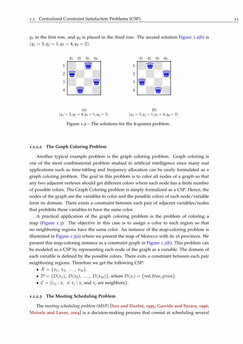
1.1. Centralized Constraint Satisfaction Problems (CSP) 11
q3 in the first row, and q4 is placed in the third row. The second solution Figure 1.2(b) is
(q1 = 3, q2 = 1, q3 = 4, q4 = 2).
q1 q2 q3 q4
1 zZz5™Xqz2 5XqzZzzZ3 zZzzZ5Xq4 z5™XqzzZ
(a)(q1 = 2, q2 = 4, q3 = 1, q4 = 3)
q1 q2 q3 q4
1 zZ5XqzZz2 zzZz5™Xq3 5™XqzzZz4 zzZ5XqzZ
(b)(q1 = 3, q2 = 1, q3 = 4, q4 = 2)
Figure 1.2 – The solutions for the 4-queens problem.
1.1.2.2 The Graph Coloring Problem
Another typical example problem is the graph coloring problem. Graph coloring is
one of the most combinatorial problem studied in artificial intelligence since many real
applications such as time-tabling and frequency allocation can be easily formulated as a
graph coloring problem. The goal in this problem is to color all nodes of a graph so that
any two adjacent vertexes should get different colors where each node has a finite number
of possible colors. The Graph Coloring problem is simply formalized as a CSP. Hence, the
nodes of the graph are the variables to color and the possible colors of each node/variable
form its domain. There exists a constraint between each pair of adjacent variables/nodes
that prohibits these variables to have the same color.
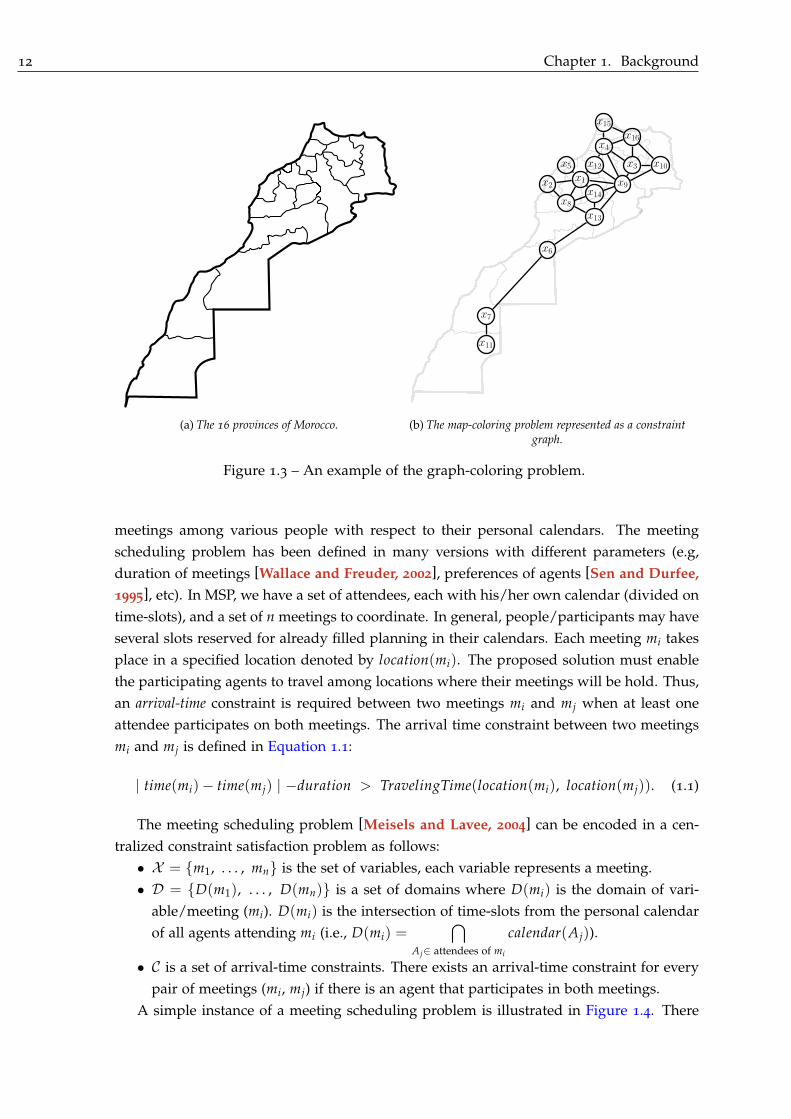
A practical application of the graph coloring problem is the problem of coloring a
map (Figure 1.3). The objective in this case is to assign a color to each region so that
no neighboring regions have the same color. An instance of the map-coloring problem is
illustrated in Figure 1.3(a) where we present the map of Morocco with its 16 provinces. We
present this map-coloring instance as a constraint graph in Figure 1.3(b). This problem can
be modeled as a CSP by representing each node of the graph as a variable. The domain of
each variable is defined by the possible colors. There exits a constraint between each pair
neighboring regions. Therefore we get the following CSP:
• X = {x1, x2, . . . , x16}.
• D = {D(x1), D(x2), . . . , D(x16)}, where D(xi) = {red, blue, green}.
• C = {cij : xi �= xj | xi and xj are neighbors}.
1.1.2.3 The Meeting Scheduling Problem
The meeting scheduling problem (MSP) [Sen and Durfee, 1995; Garrido and Sycara, 1996;
Meisels and Lavee, 2004] is a decision-making process that consist at scheduling several
12 Chapter 1. Background
(a) The 16 provinces of Morocco.
x11
x7
x6
x13
x8
x14
x9x2x1
x5 x12 x3 x10
x4
x16
x15
(b) The map-coloring problem represented as a constraintgraph.
Figure 1.3 – An example of the graph-coloring problem.
meetings among various people with respect to their personal calendars. The meeting
scheduling problem has been defined in many versions with different parameters (e.g,
duration of meetings [Wallace and Freuder, 2002], preferences of agents [Sen and Durfee,
1995], etc). In MSP, we have a set of attendees, each with his/her own calendar (divided on
time-slots), and a set of n meetings to coordinate. In general, people/participants may have
several slots reserved for already filled planning in their calendars. Each meeting mi takes
place in a specified location denoted by location(mi). The proposed solution must enable
the participating agents to travel among locations where their meetings will be hold. Thus,
an arrival-time constraint is required between two meetings mi and mj when at least one
attendee participates on both meetings. The arrival time constraint between two meetings
mi and mj is defined in Equation 1.1:
| time(mi)− time(mj) | −duration > TravelingTime(location(mi), location(mj)). (1.1)
The meeting scheduling problem [Meisels and Lavee, 2004] can be encoded in a cen-
tralized constraint satisfaction problem as follows:
• X = {m1, . . . , mn} is the set of variables, each variable represents a meeting.
• D = {D(m1), . . . , D(mn)} is a set of domains where D(mi) is the domain of vari-
able/meeting (mi). D(mi) is the intersection of time-slots from the personal calendar
of all agents attending mi (i.e., D(mi) =�
Aj∈ attendees of mi
calendar(Aj)).
• C is a set of arrival-time constraints. There exists an arrival-time constraint for every
pair of meetings (mi, mj) if there is an agent that participates in both meetings.
A simple instance of a meeting scheduling problem is illustrated in Figure 1.4. There

1.2. Algorithms and Techniques for Solving Centralized CSPs 13
m11
m13
m14
m21
m22
m32
m33
m34
m44
�=
�=�=
meeting 1
meeting 2
meeting 3
meeting 4
meeting 4
meeting 4
Med
Alice
Fred
Adam
August 2011
1 2 3 4 5 6 7
8 9 10 11 12 13 14
August 2011
1 2 3 4 5 6 7
8 9 10 11 12 13 14
August 2011
1 2 3 4 5 6 7
8 9 10 11 12 13 14
August 2011
1 2 3 4 5 6 7
8 9 10 11 12 13 14
Figure 1.4 – A simple instance of the meeting scheduling problem.
are 4 attendees: Adam, Alice, Fred and Med, each having its personal calendar. There are
4 meetings to be scheduled. The first meeting (m1) will be attended by Alice and Med.
Alice and Fred will participate on the second meeting (m2). The agents going to attend the
third meeting (m3) are Fred and Med while the last meeting (m4) will be attended by three
persons: Adam, Fred and Med.
The instance presented in Figure 1.4 is encoded as a centralized CSP in Figure 1.5. The
nodes are the meetings/variables (m1, m2, m3, m4). The edges represent binary arrival-
time constraint. Each edge is labeled by the person, attending both meetings. Thus,
• X = {m1, m2, m3, m4}.
• D = {D(m1), D(m2), D(m3), D(m4)}.
– D(m1) = {s | s is a slot in calendar(Alice) ∩ calendar(Med)}.
– D(m2) = {s | s is a slot in calendar(Alice) ∩ calendar(Fred)}.
– D(m3) = {s | s is a slot in calendar(Adam) ∩ calendar(Fred) ∩ calendar(Med)}.
– D(m4) = {s | s is a slot in calendar(Adam) ∩ calendar(Fred) ∩ calendar(Med)}.
• C = {c12, c13, c14, c23, c24, c34}, where cij is an arrival-time constraint between mi
and mj.
These examples show the power of the CSP paradigm to easily model different combi-
natorial problems arising from different issues. In the following section, we describe the
main generic methods for solving a constraint satisfaction problem.
1.2 Algorithms and Techniques for Solving Centralized CSPs
In this section, we describe the basic methods for solving constraint satisfaction prob-
lems. These methods can be considered under two board approaches: constraint propaga-
tion and search. We also describe here a combination of those two approaches. In general,

14 Chapter 1. Background
m1 m2
m3m4
Alice
Med
Med Fred
Fred
Med, Fred, Adam
Med attends meetings: m1, m2 and m4
Alice attends meetings: m1 and m2
Fred attends meetings: m2, m3 and m4
Adam attends meetings: m4
Figure 1.5 – The constraint graph of the meeting-scheduling problem.
the search algorithms explore all possible combinations of values for the variables in order
to find a solution of the problem, that is, a combination of values for the variables that
satisfies the constraints. However, the constraint propagation techniques are used to re-
duce the space of combinations that will be explored by the search process. Afterwards,
we present the main heuristics used to boost the search in the centralized CSPs. We partic-
ularly summarize the main variable ordering heuristics while we briefly describe the main
value ordering heuristics used in the constraint satisfaction problems.
1.2.1 Algorithms for solving centralized CSPs
Usually, algorithms for solving centralized CSPs search systematically through the pos-
sible assignments of values to variables in order to find a combination of these assignments
that satisfies the constraints of the problem.
Definition 1.5 An assignment of value vi to a variable xi is a pair (xi, vi) where vi is a value
from the domain of xi (i.e., vi ∈ D(xi)). We often denote this assignment by xi = vi.
Henceforth, when a variable is assigned a value from its domain, we say that the vari-
able is assigned or instantiated.
Definition 1.6 An instantiation I of a subset of variables {xi, . . . , xk} ⊆ X is an ordered set
of assignments I = {[(xi = vi), . . . , (xk = vk)] | vj ∈ D(xj)}. The variables assigned on an
instantiation I = [(xi = vi), . . . , (xk = vk)] are denoted by vars(I) = {xi, . . . , xk}.
Definition 1.7 A full instantiation is an instantiation I that instantiates all the variables of the
problem (i.e., vars(I) = X ) and conversely we say that an instantiation is a partial instantia-
tion if it instantiates in only a part.
Definition 1.8 An instantiation I satisfies a constraint cij ∈ C if and only if the variables involved
in cij (i.e., xi and xj) are assigned in I (i.e., (xi = vi), (xj = vj) ∈ I) and the pair (vi, vj) is allowed
by cij. Formally, I satisfies cij iff (xi = vi) ∈ I ∧ (xj = vj) ∈ I ∧ (vi, vj) ∈ cij.
Definition 1.9 An instantiation I is locally consistent iff it satisfies all of the constraints whose

1.2. Algorithms and Techniques for Solving Centralized CSPs 15
scopes have no uninstantiated variables in I. I is also called a partial solution. Formally,
I is locally consistent iff ∀cij ∈ C | scope(cij) ⊆ vars(I), I satisfies cij.
Definition 1.10 A solution to a constraint network is a full instantiation I, which is locally
consistent.
The intuitive way to search a solution for a constraint satisfaction problem is to generate
and test all possible combinations of the variable assignments to see if it satisfies all the
constraints. The first combination satisfying all the constraints is then a solution. This is the
principle of the generate & test algorithm. In other words, a full instantiation is generated
and then tested if it is locally consistent. In the generate & test algorithm, the consistency of
an instantiation is not checked until it is full. This method drastically increases the number
of combinations that will be generated. (The number of full instantiation considered by
this algorithm is the size of the Cartesian product of all the variable domains). Intuitively,
one can check the local consistency of instantiation as soon as its respective variables are
instantiated. In fact, this is systematic search strategy of the chronological backtracking
algorithm. We present the chronological backtracking in the following.
1.2.1.1 Chronological Backtracking (BT)
The chronological backtracking [Davis et al., 1962; Golomb and Baumert, 1965;
Bitner and Reingold, 1975] is the basic systematic search algorithm for solving CSPs. The
Backtracking (BT) is a recursive search procedure that incrementally attempts to extend a
current partial solution (a locally consistent instantiation) by assigning values to variables
not yet assigned, toward a full instantiation. However, when all values of a variable are
inconsistent with previously assigned variables (a dead-end occurs) BT backtracks to the
variable immediately instantiated in order to try another alternative value for it.
Definition 1.11 When no value is possible for a variable, a dead-end state occurs. We usually say
that the domain of the variable is wiped out (DWO).
Algorithm 1.1: The chronological Backtracking algorithm.procedure Backtracking(I)01. if ( isFull(I) ) then return I as solution; /* all variables are assigned in I */02. else03. select xi in X \ vars(I) ; /* let xi be an unassigned variable */04. foreach ( vi ∈ D(xi) ) do05. xi ← vi;06. if ( isLocallyConsistent(I ∪ {(xi = vi)}) ) then07. Backtracking(I ∪ {(xi = vi)});
The pseudo-code of the Backtracking (BT) algorithm is illustrated in Algorithm 1.1.
The BT assigns a value to each variable in turn. When assigning a value vi to a variable xi,
the consistency of the new assignment with values assigned thus far is checked (line 6, Al-
gorithm 1.1). If the new assignment is consistent with previous assignments BT attempts to
extend these assignments by selecting another unassigned variable (line 7). Otherwise (the

16 Chapter 1. Background
new assignment violates any of the constraints), another alternative value is tested for xi if
it is possible. If all values of a variable are inconsistent with previously assigned variables
(a dead-end occurs), backtracking to the variable immediately preceding the dead-end vari-
able takes place in order to check alternative values for this variable. By the way, either a
solution is found when the last variable has been successfully assigned or BT can conclude
that no solution exist if all values of the first variable are removed.
On the one hand, it is clear that we need only linear space to perform the backtracking.
However, it requires time exponential in the number of variables for most nontrivial prob-
lems. On the other hand, the backtracking is clearly better than “generate & test” since
a subtree from the search space is pruned whenever a partial instantiation violates a con-
straint. Thus, backtracking can detect early unfruitful instantiation compared to “generate
& test”.
Although the backtracking improves the “generate & test”, it still suffer from many
drawbacks. The main one is the thrashing problem. Thrashing is the fact that the same
failure due to the same reason can be rediscovered an exponential number of times when
solving the problem. Therefore, a variety of refinements of BT have been developed in
order to improve it. These improvements can be classified under two main schemes: look-
back methods as conflict directed backjumping or look-ahead methods such as forward
checking.
1.2.1.2 Conflict-directed Backjumping (CBJ)
From the earliest works in the area of constraint programming, researchers were con-
cerned by the trashing problem of the Backtracking, and then proposed a number of tools
to avoid it. backjumping concept was one of the pioneer tools used for this reason. Thus,
several non-chronological backtracking (intelligent backtracking) search algorithms have
been designed to solve centralized CSPs. In the standard form of backtracking, each time
a dead-end occurs the algorithm attempts to change the value of the most recently instan-
tiated variable. However, backtracking chronologically to the most recently instantiated
variable may not address the reason for the failure. This is no longer the case in the back-
jumping algorithms that identify and then jump directly to the responsible of the dead-end
(culprit). Hence, the culprit variable is re-assigned if it is possible or an other jump is
performed. By the way, the subtree of the search space where the thrashing may occur is
pruned.
Definition 1.12 Given a total ordering on variables O, a constraint cij is earlier than ckl if the
latest variable in scope(cij) precedes the latest one in scope(ckl) on O.
Example 1.1 Given the lexicographic ordering on variables ([x1, . . . , xn]), the constraint c25
is earlier than constraint c35 because x2 precedes x3 since x5 belongs to both scopes (i.e.,
scope(c25) and scope(c35)).
Gaschnig designed the first explicit non-chronological (backjumping) algorithm (BJ) in[Gaschnig, 1978]. BJ records for each variable xi the deepest variable with which it checks

1.2. Algorithms and Techniques for Solving Centralized CSPs 17
its consistency with the assignment of xi. When a dead-end occurs on a domain of a
variable xi, BJ jumps back to the deepest variable, say xj, to witch the consistency of xi
is checked against. However, if there are no more values remaining for xj, BJ perform
a simple backtrack to the last assigned variable before assigning xj. Dechter presented
in [Dechter, 1990; Dechter and Frost, 2002] the Graph-based BackJumping (GBJ) algorithm,
a generalization of the BJ algorithm. Basically, GBJ attempts to jump back directly to
the source of the failure by using only information extracted from the constraint graph.
Whenever a dead-end occurs on a domain of the current variable xi, GBJ jumps back to
the most recent assigned variable (xj) adjacent to xi in the constraint graph. Unlike BJ, if
a dead-end occurs again on a domain of xj, GBJ jumps back to the most recent variable xk
connected to xi or xj. Prosser proposed the Conflict-directed BackJumping (CBJ) that rectify
the bad behavior of Gaschnig’s algorithm in [Prosser, 1993].
Algorithm 1.2: The Conflict-Directed Backjumping algorithm.procedure CBJ(I)01. if ( isFull(I) ) then return I as solution; /* all variables are assigned in I */02. else03. choose xi in X \ vars(I) ; /* let xi be an unassigned variable */04. EMCS[i] ← ∅ ;05. D(xi) ← D0(xi) ;06. foreach ( vi ∈ D(xi) ) do07. xi ← vi;08. if ( isConsistent(I ∪ (xi = vi)) ) then09. CS ← CBJ(I ∪ {(xi = vi)}) ;10. if ( xi /∈ CS ) then return CS ;11. else EMCS[i] ← EMCS[i] ∪ CS \ {xi} ;12. else13. remove vi from D(xi) ;14. let cij be the earliest violated constraint by (xi = vi);15. EMCS[i] ← EMCS[i] ∪ xj ;16. return EMCS[i] ;
The pseudo-code of CBJ is illustrated in Algorithm 1.2. Instead of recording only the
(deepest variable, CBJ records for each variable xi the set of variables that were in conflict
with some assignment of xi. Thus, CBJ maintains a set of earliest minimal conflict set for each
variable xi (i.e., EMCS[i]) where it stores the variables belonging to the earliest violated
constraints with an assignment of xi. Whenever a variable xi is chosen to be instantiated
(line 3), CBJ initializes EMCS[i] to the empty set. Next, CBJ initializes the current domain
of xi to its initial domain (line 5). Afterward, a consistent value vi with the current search
state is looked for variable xi. If vi is inconsistent with the current partial solution, then vi
is removed from current domain D(xi) (line 13), and xj such that cij is the earliest violated
constraint by the new assignment of xi (i.e., xi = vi) is then added to the earliest minimal
conflict set of xi, i.e., EMCS[i] (line 15). EMCS[i] can be seen as the subset of the past
variables in conflict with xi. When a dead-end occurs on the domain of a variable xi, CBJ
jumps back to the last variable, say xj, in EMCS[i] (lines 16,9 and line 10). The information
in EMCS[i] is earned upwards to EMCS[j] (line 11). Hence, CBJ performs a form of “in-

18 Chapter 1. Background
telligent backtracking” to the source of the conflict allowing the search procedure to avoid
rediscovering the same failure due to the same reason.
When a dead-end occurs, the CBJ algorithm jumps back to address the culprit vari-
able. During the backjumping process CBJ erases all assignments that were obtained since
and then wastes a meaningful effort done to achieve these assignments. To overcome this
drawback Ginsberg (1993) have proposed Dynamic Backtracking.
1.2.1.3 Dynamic Backtracking (DBT)
In the naive chronological of backtracking (BT), each time a dead-end occurs the algo-
rithm attempts to change the value of the most recently instantiated variable. Intelligent
backtracking algorithms were developed to avoid the trashing problem caused by the BT.
Although, these algorithms identify and then jump directly to the responsible of the dead-
end (culprit), they erase a great deal of the work performed thus far on the variables that
are backjumped over. When backjumping, all variables between the culprit of the dead-end
and the variable where the dead-end occurs will be re-assigned. Ginsberg (1993) proposed
the Dynamic Backtracking algorithm (DBT) in order to keep the progress performed before
the backjumping. In DBT, the assignments of non conflicting variables are preserved dur-
ing the backjumping process. Thus, the assignments of all variables following the culprit
are kept and the culprit variable is moved to be the last among the assigned variables.
In order to detect the culprit of the dead-end, CBJ associates a conflict set (EMCS[i]) to
each variable (xi). EMCS[i] contains the set of the assigned variables whose assignments
are in conflict with a value from the domain of xi. In a similar way, DBT uses nogoods to
justify the value elimination [Ginsberg, 1993]. Based on the constraints of the problem, a
search procedure can infer inconsistent sets of assignments called nogoods.
Definition 1.13 A nogood is a conjunction of individual assignments, which has been found
inconsistent, either because the initial constraints or because searching all possible combinations.
Example 1.2 The following nogood ¬[(xi = vi)∧ (xj = vj)∧ . . .∧ (xk = vk)] means that as-
signments it contains are not simultaneously allowed because they cause an inconsistency.
Definition 1.14 A directed nogood ruling out value vk from the initial domain of variable xk is
a clause of the form xi = vi ∧ xj = vj ∧ . . . → xk �= vk, meaning that the assignment xk = vk is
inconsistent with the assignments xi = vi, xj = vj, . . .. When a nogood (ng) is represented as an
implication, the left hand side, lhs(ng), and the right hand side, rhs(ng), are defined from the
position of →.
In DBT, when a value is found to be inconsistent with previously assigned values, a
directed nogood is stored as a justification of its removal. Hence, the current domain D(xi)
of a variable xi contains all values from its initial domain that are not ruled out by a stored
nogood. When all values of a variable xi are ruled out by some nogoods, a dead-end
occurs, DBT resolves these nogoods producing a new nogood (newNogood). Let xj be the
most recent variable in the left-hand side of all these nogoods and xj = vj, that is xj is
the culprit variable in the CBJ algorithm. The lhs(newNogood) is the conjunction of the

1.2. Algorithms and Techniques for Solving Centralized CSPs 19
left-hand sides of all nogoods except xj = vj and rhs(newNogood) is xj �= vj. Unlike the
CBJ, DBT only removes the current assignment of xj and keeps assignments of all variables
between it an xi since they are consistent with former assignments. Therefore, the work
done when assigning these variables is preserved. The culprit variable xj is then placed
after xi and a new assignment for it is searched since the generated nogood (newNogood)
eliminates its current value (vj).
Since the number of nogoods that can be generated increases monotonically, recording
all of the nogoods as is done in Dependency Directed Backtracking algorithm [Stallman
and Sussman, 1977] requires an exponential space complexity. In order to keep a polyno-
mial space complexity, DBT stores only nogoods compatible with the current state of the
search. Thus, when backtracking to xj, DBT destroys all nogoods containing xj = vj. As a
result, with this approach a variable assignment can be ruled out by at most one nogood.
Since each nogood requires O(n) space and there are at most nd nogoods, where n is the
number of variables and d is the maximum domain size, the overall space complexity of
DBT is in O(n2d).
1.2.1.4 Partial Order Dynamic Backtracking (PODB)
Instead of backtracking to the most recently assigned variable in the nogood, Ginsberg
and McAllester proposed the Partial Order Dynamic Backtracking (PODB), an algorithm that
offers more freedom than DBT in the selection of the variable to put on the right-hand side
of the directed nogood [Ginsberg and McAllester, 1994]. thereby, PODB is a polynomial
space algorithm that attempted to address the rigidity of dynamic backtracking.
When resolving the nogoods that lead to a dead-end, DBT always select the most among
the set of inconsistent assignments recent assigned variable to be the right hand side of the
generated directed nogood. However, there are clearly many different ways of representing
a given nogood as an implication (directed nogood). For example, ¬[(xi = vi)∧ (xj = vj)∧
· · · ∧ (xk = vk)] is logically equivalent to [(xj = vj) ∧ · · · ∧ (xk = vk)] → (xi �= vi) meaning
that the assignment xi = vi is inconsistent with the assignments xj = vj, . . . , xk = vk.
Each directed nogood imposes ordering constraints, called the set of safety conditions for
completeness [Ginsberg and McAllester, 1994]. Since all variables in the left hand side of
a directed nogood participate in eliminating the value on its right hand side, these variable
must precede the variable on the right hand side.
Definition 1.15 safety conditions imposed by a directed nogood (ng) ruling out a value from the
domain of xj are the set of assertions of the form xk ≺ xj where xk is a variable in the left hand side
of ng (i.e., xk ∈ vars(lhs(ng))).
The Partial Order Dynamic Backtracking attempts to offer more freedom in the selection
of the variable to put on the right-hand side of the generated directed nogood. In PODB, the
only restriction to respect is that the partial order induced by the resulting directed nogood
must safety the existing partial order required by the set of safety conditions, say S. In a
later study, Bliek shows that PODB is not a generalization of DBT and then proposes the
Generalized Partial Order Dynamic Backtracking (GPODB), a new algorithm that generalizes

20 Chapter 1. Background
both PODB and DBT [Bliek, 1998]. To achieve this, GPODB follows the same mechanism of
PODB. The difference between two resides in the obtained set of safety conditions S� after
generating a new directed nogood (newNogood). The new order has to respect the safety
conditions existing in S�. While S and S� are the similar for PODB, when computing S�
GPODB relaxes from S all safety conditions of the form rhs(newNogood) ≺ xk. However,
both algorithms generates only directed nogoods that satisfy the already existing safety
conditions in S. In the best of our knowledge, no systematic evaluation of either PODB or
GPODB have been reported.
All algorithms presented previously incorporates a form of look-back scheme. Avoid-
ing possible future conflicts may be more attractive than recovering from them. In the
backtracking, backjumping and dynamic backtracking, we can not detect that an instan-
tiation is unfruitful till all variables of the conflicting constraint are assigned. Intuitively,
each time a new assignment is added to the current partial solution, one can look ahead by
performing a forward check of consistency of the current partial solution.
1.2.1.5 Forward Checking (FC)
The forward checking (FC) algorithm [Haralick and Elliott, 1979; Haralick and Elliott,
1980] is the simplest procedure of checking every new instantiation against the future
(as yet uninstantiated) variables. The purpose of the forward checking is to propagate
information from assigned to unassigned variables. Then, it is classified among those
procedures performing a look-ahead.
Algorithm 1.3: The forward checking algorithm.procedure ForwardChecking(I)01. if ( isFull(I) ) then return I as solution; /* all variables are assigned in I */02. else03. select xi in X \ vars(I) ; /* let xi be an unassigned variable */04. foreach ( vi ∈ D(xi) ) do05. xi ← vi;06. if ( Check-Forward(I, (xi = vi)) ) then07. ForwardChecking(I ∪ {(xi = vi)});08. else09. foreach ( xj /∈ vars(I) such that ∃ cij ∈ C ) do restore D(xj);
function Check-Forward(I, xi = vi)
10. foreach ( xj /∈ vars(I) such that ∃ cij ∈ C ) do
11. foreach ( vj ∈ D(xj) such that (vi , vj) /∈ cij ) do remove vj from D(xj) ;12. if ( D(xj) = ∅ ) then return false;13. return true;
The pseudo-code of FC procedure is presented in Algorithm 1.3. FC is a recursive
procedure that attempts to foresee the effects of choosing an assignment on the not yet
assigned variables. Each time a variable is assigned, FC checks forward the effects of this
assignment on the future variables domains (Check-Forward call, line 6). So, all values
from the domains of future variables which are inconsistent with the assigned value (vi) of
the current variable (xi) are removed (line 11). Future variables concerned by this filtering
1.2. Algorithms and Techniques for Solving Centralized CSPs 21
process are only those sharing a constraint with xi, the current variable being instantiated
(line 10). By the way, each domain of a future variable is filtered in order to keep only
consistent values with past variables (variables already instantiated). Hence, FC does not
need to check consistency of new assignments against already instantiated ones as opposed
to chronological backtracking. The forward checking is then the easiest way to prevent
assignments that guarantee later failure.
Unlike backtracking, forward checking algorithm enables to prevent assignments that
guarantee later failure. This improves the performance of backtracking. However, forward
checking reduces the domains of future variables checking only the constraints relating
them to variables already instantiated. In addition to these constraints, one can checks also
the constraints relating future variables to each other. By the way, domains of future vari-
ables may be reduced and further possible conflicts will be avoided. This is the principle of
the full look-ahead scheme or constraint propagation. This approach is called maintaining
arc consistency (MAC).
1.2.1.6 Arc-consistency (AC)
In constraint satisfaction problems, checking the existence of solutions is NP-complete.
Therefore, the research community has devoted a great interest in studying the constraint
propagation techniques. Constraint propagation techniques are filtering mechanisms that
aim to improve the performance of the search process by attempting to reduce the search
space. They have been widely used to simplify the search space before or during the
search of solutions. Thus, constraint propagation became a central process of solving CSPs[Bessiere, 2006]. Historically, different kinds of constraint propagation techniques have
been proposed: node consistency [Mackworth, 1977], arc consistency [Mackworth, 1977]
and path consistency [Montanari, 1974] . The oldest and most commonly used technique
for propagating constraints in literature is the Arc Consistency, AC.
Definition 1.16 A value vi ∈ D(xi) is consistent with cij in D(xj) iff there exists a value vj ∈
D(xj) such that (vi, vj) is allowed by cij. Value vj is called a support for vi in D(xj).
Let us assume the constraint graph G = {XG, EG} (see Definition 1.2) associated to our
constraint satisfaction problem.
Definition 1.17 An arc {xi, xj} ∈ EG (constraint cij) is arc consistent iff ∀ vi ∈ D(xi), ∃ vj ∈
D(xj) such that (vi, vj) is allowed by cij and ∀ vj ∈ D(xj), ∃ vi ∈ D(xi) such that (vi, vj) is
allowed by cij. A constraint network is arc consistent iff all its arcs (constraints) are arc consistent.
A constraint network is arc consistent if and only if for any value vi in the domain,
D(xi), of a variable xi there exist in the domain D(xj) of an adjacent variable xj a value
vj that is compatible with vi. Clearly, if an arc {xi, xj} (i.e., a constraint cij) is not arc
consistent, it can be made arc consistent by simply deleting all values from the domains
of the variables in its scope for which there is not a support in the other domain. It is
obvious that these deletions maintains the problem solutions since the deleted values are
in no solution. The process of removing values from the domain of a variable xi, when

22 Chapter 1. Background
making an arc {xi, xj} arc consistent is called revising D(xi) with respect to constraint cij.
A wide variety of algorithms establishing arc consistency on CSPs have been developed:
AC-3 [Mackworth, 1977], AC-4 [Mohr and Henderson, 1986], AC-5 [Van Hentenryck et
al., 1992], AC-6 [Bessiere and Cordier, 1993; Bessiere, 1994], AC-7 [Bessiere et al., 1999],
AC-2001 [Bessiere and Régin, 2001], etc. The basic algorithm and the most will-known
one is Mackworth’s AC-3.
Algorithm 1.4: The AC-3 algorithm.function Revise(xi , xj)
01. change ← false;02. foreach ( vi ∈ D(xi) ) do03. if ( � vj ∈ D(xj) such that (vi , vj) ∈ cij ) then
04. remove vi from D(xi) ;05. change ← true;06. return change ;function AC-3()
07. foreach ( {xi , xj} ∈ EG ) do /* {xi , xj} ∈ EG iff ∃ cij ∈ C */08. Q ← Q ∪ {(xi , xj); (xj, xi)} ;09. while ( Q �= ∅ ) do10. (xi , xj) ← Q.pop() ; /* Select and remove (xi , xj) from Q */11. if ( Revise(xi , xj) ) then
12. if ( D(xi) = ∅ ) then return false ; /* The problem is unsatisfiable */13. else Q ← Q ∪ { (xk , xi) | {xk , xi} ∈ EG , k �= i, k �= j } ;14. return true ; /* The problem is arc consistent */
We illustrate the AC-3 algorithm in Algorithm 1.4. The AC-3 algorithm maintains a
queue Q 1 of arcs to render arc consistent. AC-3 algorithm will return true once the problem
is made arc consistent or false if an empty domain was generated (a domain is wiped out)
meaning that the problem is not satisfiable. Initially, Q is filled with all ordered pair of
variables that participates in a constraint. Thus, for each constraint cij ({xi, xj}) we add
to Q the ordered pair (xi, xj) to revise the domain of xi and the ordered pair (xj, xi) the
revise the domain of xj (line 8). Next, the algorithm loops until it is guaranteed that all arcs
have been made arc consistent (i.e., while Q is not empty). The ordered pair of variables
are selected and removed one by one from Q to revise the domain of the first variable.
Each time an ordered pair of variable (xi, xj) is selected and removed from Q (line 10),
AC-3 calls function Revise(xi, xj) to revise the domain of xi. When revising D(xi) with
respect to an arc {xi, xj} (Revise call, line 11), all values that are not consistent with cij
are removes from D(xi) (lines 2-4). Thus, only values having a support on D(xj) are kept
in D(xi). The function Revise returns true if the domain of variable xi has been reduced,
false otherwise (line 6). If Revise results in the removal of values from D(xi) it can be the
case that a value for another variable xk has lost its support on D(xi). Thus, all ordered
pairs (xk, xi) such that k �= j are added onto Q so long as they are not already on Q in order
to revise the domain of xk. Obviously, the AC-3 algorithm will not terminate as long as
there is any pair in Q. When Q is empty, we are guaranteed that all arcs have been made
arc consistent. Hence, the constraint network is arc consistent. The while loop of AC-3 can
1. Other data structures as queue or stack can perfectly serve the purpose

1.2. Algorithms and Techniques for Solving Centralized CSPs 23
be intuitively understood as constraint propagation (i.e., propagation the effect of value
removals on other domains potentially affected by these removals).
1.2.1.7 Maintaining Arc-Consistency (MAC)
Historically, constraint propagation techniques are used in a preprocessing step to
prune values before search. Thus, the search space that will be explored by the search algo-
rithm is reduced since domains of all variables are refined. By the way, subsequent search
efforts by the solution method will be reduced. Afterward, the search method can be called
for searching a solution. Constraint propagation techniques are also used during search.
This strategy is that used by the forward checking algorithm. Forward checking combines
backtrack search with a limited form of arc consistency maintenance on the domains of fu-
ture variables. Instead of performing a limited form of arc consistency, Sabin and Freuder
proposed in [Sabin and Freuder, 1994] the Maintaining Arc-Consistency (MAC) algorithm
that established and maintained a full arc consistency on the domains of future variables.
The Maintaining Arc Consistency (MAC) algorithm is a modern version of CS2 algorithm[Gaschnig, 1974]. MAC alternates the search process and constraint propagation steps as
is done in forward checking [Haralick and Elliott, 1980]. Nevertheless, before starting
the search method, MAC makes the constraint network arc consistent. In addition, when
instantiating a variable xi to a value vi, all the other values in D(xi) are removed and
the effects of these removals are propagated through the constraint network [Sabin and
Freuder, 1994]. The maintaining arc consistency algorithm enforces arc consistency in the
search process as follows. At each step of the search, a variable assignment is followed by a
filtering process that corresponds to enforcing arc consistency. Therefore, MAC maintains
the arc consistency each time an instantiation is added to the partial solution. In other
word, whenever a value vi is instantiated to a variable xi, D(xi) is reduced momentarily to
a single value vi (i.e., D(xi) ← {vi}) and the resulting constraint network is then made arc
consistent.
1.2.2 Variable Ordering Heuristics for Centralized CSP
Numerous efficient search algorithms for solving constraint satisfaction problems have
been developed. The performance of these algorithms were evaluated in different stud-
ies and then shown to be powerful tools for solving CSPs. Nevertheless, since CSPs are
in general NP-complete, these algorithms still exponential. Therefore, a large variety of
heuristics were developed to improve their efficiency. That is, search algorithms solving
CSPs are commonly combined with heuristics for boosting the search. The literature is rich
in heuristics designed for this task. The order in which variables are assigned by a search
algorithm was one of the early concern for these heuristics. The order on variables can be
either static or dynamic.

24 Chapter 1. Background
1.2.2.1 Static Variable Ordering Heuristics (SVO)
The first kind of heuristics addressing the ordering of variables was based on the initial
structure of the network. Thus, the order of the variables can be determined prior the
search of solution. These heuristics are called Static Variable Ordering heuristics (SVO).
When presenting the main search procedures (Section 1.2), we always assumed without
specifying it each time, a static variable ordering. Therefore, in the previous examples we
have always used the lexicographic ordering of variables. That lexicographic ordering can
be simply replaced by an other ordering more appropriate to the structure of the network
before starting search.
Static variable ordering heuristics (SVO) are heuristics that keep the same ordering all
along the search. Hence, the ordering computed on a preprocessing step only exploit (struc-
tural) information about the initial state of the search. Examples of such SVO heuristics
are:
min-width The minimum width heuristic [Freuder, 1982] chooses an ordering that mini-
mizes the width of the constraint graph. The width of an ordering O is the maxi-
mum number of neighbors of any variable xi that occur earlier than xi under O. The
width of a constraint graph is the minimum width over all orderings of variables of
that graph. Minimizing the width of the constraint graph G can be accomplished
by a greedy algorithm. Hence, variables are ordered from last to first by choosing,
at each step, a variable having the minimum number of neighbors (min degree) in
the remaining constraint graph after deleting from the constraint graph all variables
which have been already ordered.
max-degree The maximum degree heuristic [Dechter and Meiri, 1989] orders the vari-
ables in a decreasing order of their degrees in the constraint graph (i.e., the size
of their neighborhood). This heuristic also aims at, without any guarantee, finding a
minimum-width ordering.
max-cardinality The maximum cardinality heuristic [Dechter and Meiri, 1989] orders the
variables according to the initial size of their neighborhood. max-cardinality puts
in the first position of the resulting ordering an arbitrarily variable. Afterward,
other variables are ordered from second to last by choosing, at each step, the most
connected variable with previously ordered variables. In a particular case, max-
cardinality may choose as the first variable the one that has the largest number of
neighbors.
min-bandwidth The minimum bandwidth heuristic [Zabih, 1990] minimizes the bandwidth
of the constraint graph. The bandwidth of an ordering is the maximum distance
between any two adjacent variables in the ordering. The bandwidth of a constraint
graph is the minimum bandwidth over all orderings on variables of that graph. Zabih
claims that an ordering with a small bandwidth will reduce the need for backjump-
ing because the culprit variable will be close to the variable where a dead-end occurs.
Many heuristic procedures for finding minimum bandwidth orderings have been de-
veloped, a survey of these procedures is given in [Chinn et al., 1982]. However, there

1.2. Algorithms and Techniques for Solving Centralized CSPs 25
is currently little empirical evidence that min-bandwidth is an effective heuristic.
Moreover, bandwidth minimization is NP-complete.
Another static variable ordering heuristic that tries to exploit the structural information
residing in the constraint graph is presented in [Freuder and Quinn, 1985]. Freuder and
Quinn (1985) have introduced the use of pseudo-tree arrangement of a constraint graph in
order to enhance the research complexity in centralized constraint satisfaction problems.
Definition 1.18 A pseudo-tree arrangement T = (XT , ET) of a constraint graph G = (XG, EG)
is a rooted tree with the same set of vertexes as G (i.e., XG = XT) such that vertexes in different
branches of T do not share any edge in G.
The concept of pseudo-tree arrangement of a constraint graph has been introduced first
by Freuder and Quinn in [Freuder and Quinn, 1985]. The purpose of this arrangement is to
perform search in parallel on independent branches of the pseudo-tree in order to improve
search in centralized CSPs. A recursive procedure for heuristically building pseudo-trees
have been presented by Freuder and Quinn in [Freuder and Quinn, 1985]. The heuristic
aims to select from GX the minimal subset of vertexes named cutset whose removal divides
G into disconnected sub-graphs. The selected cutset will form the first levels of the pseudo-
tree while next levels are build by recursively applying the procedure to the disconnected
sub-graphs obtained previously. By the way, the connected vertexes in the constraint graph
G belongs to the same branch of the obtained tree. Thus, the tree obtained is a pseudo-tree
arrangement of the constraint graph. Once, the pseudo-tree arrangement of the constraint
graph is built, several search procedure can be performed in parallel on each branch of the
pseudo-tree.
Although static variable ordering heuristics are undoubtedly cheaper since they are
computed once and for all, using this kind of variable ordering heuristics does not change
the worst-case complexity of the classical search algorithms. On the other hand, researchers
have been expected that dynamic variable ordering heuristics (DVO) can be more efficient.
DVO heuristics were expected to be potentially more powerful because they can take ad-
vantage from the information about the current search state.
1.2.2.2 Dynamic Variable Ordering Heuristics (DVO)
Instead of fixing an ordering as is done is SVO heuristics, dynamic variable ordering
(DVO) heuristics determines the order of the variables as search progresses. The order
of the variables may then differ from one branch of the search tree to another. It has
been shown empirically for many practical problems that DVO heuristics are more ef-
fective than choosing a good static ordering [Haralick and Elliott, 1980; Purdom, 1983;
Dechter and Meiri, 1989; Bacchus and Van Run, 1995; Gent et al., 1996]. Hence, the field
of constraint programming has so far mainly focused on such king of heuristics. There-
fore, many dynamic variable ordering heuristics for solving constraint networks have been
proposed and evaluated over the years. These heuristics are usually combined with search
procedures performing some form of look ahead (see Section 1.2.1.5 and Section 1.2.1.7) in
order to take into account changes on not yet instantiated (future) variables.

26 Chapter 1. Background
The guiding idea of the most DVO heuristic is to select the future variable with the
smallest domain size. Henceforth, this heuristic is named dom. Historically, Golomb and
Baumert (1965) where the first to propose the dom heuristic. However, it was popularized
when it was combined with the forward checking procedure by Haralick and Elliott (1980).
dom investigates the future variables (remaining sub-problem) and provides choosing as
next variable the one with the smallest remaining domain. Haralick and Elliott proposed
dom under the rubric of an intuition called fail first principle: “to succeed, try first where you
are likely to fail”. Moreover, they assume that “the best search order is the one which minimizes
the expected length or depth of each branch” (p. 308). Thus, they estimate that minimizing
branch length in a search procedure should also minimize search effort.
Many studies has gone into understanding the dom heuristic that is a simple but ef-
fective heuristic. Following the same principle of Haralick and Elliott saying that search
efficiency is due to earlier failure, Smith and Grant (1998) have derived from dom new
heuristics that detect failures earlier than dom. Their study is based on a intuitive hy-
potheses saying that earlier detection of failure should lead the heuristic to lower search
effort. Surprisingly, Smith and Grant’s experiments refuted this hypotheses contrary to
their expectations. They concluded that increasing the ability to fail early in the search
did not always lead to increased search efficiency. In follow on work, Beck et al. (2005)
shown that in forward checking (Section 1.2.1.5) minimizing branch depth is associated
with an increase in the branching factor. This can lead forward checking to perform badly.
Nevertheless, their experiments show that minimizing branch depth in Maintained Arc
Consistency (Section 1.2.1.7) reduces the search effort. Therefore, Beck et al. do not over-
look the principle of trying to fail earlier in the search. They propose to redefine failing
early in a such way to combine both the branching factor and the branch depth as it was
suggested by Nudel in [Nudel, 1983] (for instance, minimizing the number of nodes in the
failed subtrees).
In addition to the studies that has gone into understanding dom, considerable research
effort has been spent on improving it by suggesting numerous variants. These variants
express the intuitive idea that a variable which is constrained with many future variables
can also lead to a failure (a dead-end). Thus, these variants attempts to take into account
the neighborhood of the variables as well as their domain size. We present in the following
a set of well-known variable ordering heuristics derived from dom.
dom+deg A variant of dom, dom+deg, have been designed in [Frost and Dechter, 1994] to
break ties when all variables have the same initial domain size. dom+deg heuristic
breaks ties by giving priority to variable with the highest degree (i.e., the one with the
largest number of neighbors).
dom+futdeg Another variant breaking ties of dom is the dom+futdeg heuristic [Brélaz,
1979; Smith, 1999]. Originally, dom+futdeg was developed by Brélaz for the graph
coloring problem and then applied later to CSPs. dom+futdeg chooses a variable
with smallest remaining domain (dom), but in case of a tie, it chooses from these
the variable with largest future degree, that is, the one having the largest number of
neighbors in the remaining subproblem (i.e., among future variables).

1.2. Algorithms and Techniques for Solving Centralized CSPs 27
dom/deg Both dom+deg and dom+futdeg use the domain size as the main criterion. The
degree of the variables is considered only in case of ties. Alternatively, Bessiere
and Régin (1996) combined dom with deg in a new heuristics called dom/deg. The
dom/deg do not gives priority to the domain size or degree of variables but uses them
equally. This heuristic selects the variable that minimizes the ratio of current domain
size to static degree. Bessiere and Régin have been shown that dom/deg gives good
results in comparison with dom when the constraint graphs are sparse but performs
badly on dense constraint graphs. They, considered a variant of this heuristic which
minimizes the ratio of current domain size to future degree dom/futdeg. However,
they found that the performance of dom/futdeg is roughly similar to that of dom/deg.
Multi-level-DVO A general formulation of dynamic variable ordering heuristics which
approximates the constrainedness of variables and constraints, denoted Multi-level-
DVO, have been proposed in [Bessiere et al., 2001a]. Multi-level-DVO heuristics are
considered as neighborhood generalizations of dom and dom/deg and the selection
function for variable xi they suggested is as follows:
H�α (xi) =
∑xj∈Γ(xi)
(α(xi)� α(xj))
| Γ(xi) |2
where Γ(xi) is the set of xi neighbors, α(xi) can be any syntactical property of the
variable such as dom or dom/deg and � ∈ {+,×}. Therefore, Multi-level-DVO take
into account the neighborhood of variables which have shown to be quite promising.
Moreover, it allows using functions to measure the weight of a given constraint.
dom/wdeg Conflict-driven variable ordering heuristics have been introduced in [Bousse-
mart et al., 2004]. These heuristics learn from previous failures to manage the choice
on future variables. When a constraint leads to a dead-end, its weight is incremented
by one. Each variable has a weighted degree, which is the sum of the weights over all
constraints involving this variable. This heuristic can simply select the variable with
the largest weighted degree (wdeg) or incorporating the domain size of variables
to give the domain-over-weighted-degree heuristic (dom/wdeg). dom/wdeg selects
among future variables the one with minimum ratio between current domain size
and weighted degree. wdeg and dom/wdeg (especially dom/wdeg) have been shown
to perform well on a variety of problems.
In addition to the variable heuristics we presented here, other elegant dynamic
heuristics have been developed for centralized CSPs in many studies [Gent et al., 1996;
Horsch and Havens, 2000]. However, these heuristics require extra computation and have
only been tested on random problems. On other hand, it has been shown empirically
that maintaining arc-consistency (MAC) combined to the dom/deg or the dom/wdeg can
reduce or remove the need for backjumping on some problems [Bessiere and Régin, 1996;
Lecoutre et al., 2004]. Although, the variable ordering heuristics proposed are numerous,
one has to notice that none of these heuristics has been proved to be efficient in every
instance of the problems.

28 Chapter 1. Background
Beside different variable ordering heuristics designed to improve the efficiency of
search procedure, researchers developed many Look-ahead Value Ordering (LVO) heuris-
tics. This is because value ordering heuristic are powerful way of reducing the ef-
forts of search algorithms [Haralick and Elliott, 1980]. Therefore the constraint pro-
gramming community developed various LVO heuristics that choose which value to
instantiate to the selected variable. Many designed value ordering heuristics attempt
to choose next the least constraining values, i.e., values that are most likely to suc-
ceed. By the way, values that are expected to participate in many solutions are priv-
ileged. Minton et al. designed a value ordering heuristic, the min-conflicts, that at-
tempts to minimize the number of constraint violations after each step [Minton et al.,
1992]. Selecting first min-conflicts values maximizes the number of values available for
future variables. Therefore, partial solutions that cannot be extended will be avoided.
Other heuristics try to first select value maximizing the product [Ginsberg et al., 1990;
Geelen, 1992] or the sum of support in future domain after propagation [Frost and Dechter,
1995]. Nevertheless, However, all these heuristics are costly. Literature is rich on other LVO,
to mention a few [Dechter and Pearl, 1988; Frost and Dechter, 1995; Meisels et al., 1997;
Vernooy and Havens, 1999; Kask et al., 2004].
1.3 Distributed constraint satisfaction problems (DisCSP)
A wide variety of problems in artificial intelligence are solved using the constraint sat-
isfaction problem paradigm. However, there exist applications that are of a distributed
nature. In this kind of applications the knowledge about the problem, that is, vari-
ables and constraints, may be logically or geographically distributed among physical
distributed agents. This distribution is mainly due to privacy and/or security require-
ments: constraints or possible values may be strategic information that should not be
revealed to other agents that can be seen as competitors. In addition, a distributed sys-
tem provides fault tolerance, which means that if some agents disconnect, a solution
might be available for the connected part. Several applications in multi-agent coordina-
tion are of such kind. Examples of applications are sensor networks [Jung et al., 2001;
Béjar et al., 2005], military unmanned aerial vehicles teams [Jung et al., 2001], distributed
scheduling problems [Wallace and Freuder, 2002; Maheswaran et al., 2004], distributed
resource allocation problems [Petcu and Faltings, 2004], log-based reconciliation [Chong
and Hamadi, 2006], Distributed Vehicle Routing Problems [Léauté and Faltings, 2011], etc.
Therefore, a distributed model allowing a decentralized solving process is more adequate
to model and solve such kind of problems. The distributed constraint satisfaction problem has
such properties.
A Distributed Constraint Satisfaction Problem (DisCSP) is composed of a group
of autonomous agents, where each agent has control of some elements of informa-
tion about the whole problem, that is, variables and constraints. Each agent owns its
local constraint network. Variables in different agents are connected by constraints.
Agents must assign values to their variables so that all constraints are satisfied. Hence,

1.3. Distributed constraint satisfaction problems (DisCSP) 29
agents assign values to their variables, attempting to generate a locally consistent as-
signment that is also consistent with constraints between agents [Yokoo et al., 1998;
Yokoo, 2000a]. To achieve this goal, agents check the value assignments to their vari-
ables for local consistency and exchange messages among them to check consistency of
their proposed assignments against constraints that contain variables that belong to other
agents.
1.3.1 Preliminaries
The Distributed Constraint Satisfaction Problem (DisCSP) is a constraint network where
variables and constraints are distributed among multiple automated agents [Yokoo et al.,
1998].
Definition 1.19 A DisCSP (or a distributed constraint network) has been formalized as a tuple
(A,X ,D, C), where:
• A = {A1, . . . , Ap} is a set of p agents.
• X = {x1, . . . , xn} is a set of n variables such that each variable xi is controlled by one agent
in A.
• D = {D(x1), . . . , D(xn)} is a set of current domains, where D(xi) is a finite set of possible
values for variable xi.
• C = {C1, . . . , Ce} is a set of e constraints that specify the combinations of values allowed
for the variables they involve.
Values may be pruned from the domain of a variable. At any node, the set of possible
values for variable xi is its current domain, D(xi). In the same manner for centralized
CSPs, we introduce the particular notation of initial domains (or definition domains) D0 =
{D0(x1), . . . , D0(xn)}, that represents the set of domains before pruning any value (i.e.,
D ⊆ D0).
In the following, we provide some material assumptions in context of DisCSPs. First, we
assume a binary distributed constraint network where all constraints are binary constraints
(they involve two variables). A constraint cij ∈ C between two variables xi and xj is a subset
of the Cartesian product of their domains (cij ⊆ D0(xi)× D0(xj)). For simplicity purposes,
we consider a restricted version of DisCSPs where each agent controls exactly one variable
(p = n). Thus, we use the terms agent and variable interchangeably and we identify the
agent ID with its variable index. We assume also that each agent (Ai) knows all constraints
involving its variable and its neighbors (Γ(xi)) with whom it shares these constraints. We
also assume that only the agent who is assigned a variable has control on its value and
knowledge of its domain. In this thesis, we adopt the model of communication between
agents presented in [Yokoo, 2000b] where it is assumed that:
• agents communicate by exchanging messages,
• the delay in delivering a message is random but finite and
• an agent can communicate with other agents if it knows their addresses.
Initially, each agent knows addresses of all its neighbors without excluding the possi-
bility of getting addresses of other agents if it is necessary. However we discard the FIFO

30 Chapter 1. Background
assumption on communication channels between agents. Hence, we assume that commu-
nication between two agents is not necessarily generalized FIFO (aka causal order) channels[Silaghi, 2006].
Almost all distributed algorithms designed for solving distributed CSPs require a total
priority order on agents. The total order on agents is denoted by O (see Definition 1.4).
In this thesis, we present two classes of distributed algorithms with regard the agents
ordering. The first category of distributed algorithms for solving DisCSPs corresponds to
those using a static ordering on agents. The second category of distributed algorithms for
solving DisCSPs corresponds to those performing a dynamic reordering of agents during
search. For the first category of algorithms and without loss any generality, we will assume
that the total order on agents is the lexicographic ordering [A1, A2, . . . , An].
For each agent Ai ∈ A, an agent Aj has a higher priority than Ai if it appears before Ai
in the total ordering on agents. We say that xj precede xi in the ordering and we denote
this by xj ≺ xi. Conversely, Aj has a lower priority than Ai if it appears after Ai in the total
ordering on agents (i.e., xj � xi). Hence, the higher priority agents are those appearing
before Ai in O. Conversely, the lower priority agents are those appearing after Ai. As a
results, O divides the neighbors of Ai, Γ(xi), into higher priority neighbors, Γ−(xi), and
lower priority neighbors, Γ+(xi).
Instead of assuming that communication between agents is necessarily FIFO, we adopt a
model where each agent (Ai) maintains a counter that is incremented whenever Ai changes
its value. The current value of the counter tags each generated assignment.
Definition 1.20 An assignment for an agent Ai ∈ A is a tuple (xi, vi, ti), where vi is a value
from the domain of xi and ti is the tag value. When comparing two assignments, the most up to
date is the one with the greatest tag ti. Two sets of assignments {(xi1 , vi1 , ti1), . . . , (xik, vik
, tik)}
and {(xj1 , vj1 , tj1), . . . , (xjq , vjq , tjq)} are compatible if every common variable is assigned the same
value in both sets.
In order to solve distributed CSPs agents exchange their proposals with other agents.
Definition 1.21 The AgentView of an agent Ai ∈ A is an array containing the most up to date
assignments received from other agents.
1.3.2 Examples of DisCSPs
A major motivation for research on Distributed Constraint Satisfaction Problems (DisC-
SPs) is that it is an elegant model for many every day combinatorial problems arising
in Distributed Artificial Intelligence. Thus, DisCSPs have a wide range of applications in
multi-agent coordination. Sensor networks [Jung et al., 2001; Béjar et al., 2005], distributed
resource allocation problems [Prosser et al., 1992; Petcu and Faltings, 2004], distributed
meeting scheduling [Wallace and Freuder, 2002; Maheswaran et al., 2004], log-based rec-
onciliation [Chong and Hamadi, 2006] and military unmanned aerial vehicles teams [Jung
et al., 2001] are non-exhaustive examples of real applications of a distributed nature that are

1.3. Distributed constraint satisfaction problems (DisCSP) 31
successfully modeled and solved by the DisCSP framework. We present in the following
some instances of these applications.
1.3.2.1 Distributed Meeting Scheduling Problem (DisMSP)
In Section 1.1.2.3, we presented the Meeting Scheduling Problem as a centralized CSP.
Nonetheless, it is a problem of a distributed nature. The Distributed Meeting Scheduling
Problem (DisMSP) is a truly distributed problem where agents may not desire to deliver
their personal information to a centralized agent to solve the whole problem [Wallace and
Freuder, 2002; Meisels and Lavee, 2004]. The DisMSP involves a set of n agents having a
personal private calendar and a set of m meetings each taking place in a specified location.
Each agent, Ai ∈ A, knows the set of the ki among m meetings he/she must attend. It
is assumed that each agent knows the traveling time between the locations where his/her
meetings will be held. The traveling time between locations where two meetings mi and
mj will be hold is denoted by TravellingTime(mi, mj). Solving the problem consists in
satisfying the following constraints: (i) all agents attending a meeting must agree on when
it will occur, (ii) an agent cannot attend two meetings at same time, (iii) an agent must have
enough time to travel from the location where he/she is to the location where the next
meeting will be held.
Distributed Meeting Scheduling Problem (DisMSP) is encoded in DisCSP as follows.
Each DisCSP agent represents a real agent and contains k variables representing the k
meetings to which the agent participates. The domain of each variable contains the d × h
slots where a meeting can be scheduled such that there are h slots per day and d days. There
is an equality constraint for each pair of variables corresponding to the same meeting in
different agents. This equality constraint means that all agents attending a meeting must
schedule it at the same slot (constraint (i)). There is an arrival-time constraint between all
variables/meetings belonging to the same agent. The arrival-time constraint between two
variables mi and mj is defined as follows (Equation 1.2):
|mi − mj|− duration > TravellingTime(mi, mj) (1.2)
where duration is the duration of every meeting. This arrival-time constraint allows us to
express both constraints (ii) and (iii).
We illustrate in Figure 1.6 the encoding of the instance of the meeting scheduling prob-
lem shown in Figure 1.4 in the distributed constraint network formalism. This figure shows
4 agents where each agent has a personal private calendar and a set of meetings each taking
place in a specified location. Thus we get the following DisCSP:
• A = {A1, A2, A3, A4}, each agent Ai corresponds to a real agent.
• For each agent Ai ∈ A there is a variable mik, for every meeting mk that Ai attends,
X = {m11, m13, m14, m21, m22, m32, m33, m34, m44}.
• D = {D(mik) | mik ∈ X} where,
– D(m11) = D(m13) = D(m14) = {s | s is a slot in calendar(A1)}.
– D(m21) = D(m22) = {s | s is a slot in calendar(A2)}.

32 Chapter 1. Background
m11
m13
m14
m21
m22
m32
m33
m34
m44
arrival-time constraints
=
=
=
=
=
=
A1
A2
A3
A4
August 2011
1 2 3 4 5 6 7
8 9 10 11 12 13 14
August 2011
1 2 3 4 5 6 7
8 9 10 11 12 13 14
August 2011
1 2 3 4 5 6 7
8 9 10 11 12 13 14
August 2011
1 2 3 4 5 6 7
8 9 10 11 12 13 14
Figure 1.6 – The distributed meeting-scheduling problem modeled as DisCSP.
– D(m32) = D(m33) = D(m34) = {s | s is a slot in calendar(A3)}.
– D(m44) = {s | s is a slot in calendar(A4)}.
• For each agent Ai, there is a private arrival-time constraint (cikl) between every pair of
its local variables (mik, mil). For each two agents Ai, Aj that attend the same meeting
mk there is an equality inter-agent constraint (cijk ) between the variables mik and mjk,
corresponding to the meeting mk on agent Ai and Aj. Then, C = {cikl , c
ijk }.
1.3.2.2 Distributed Sensor Network Problem (SensorDCSP)
The Distributed Sensor Network Problem (SensorDisCSP) is a real distributed resource
allocation problem [Jung et al., 2001; Béjar et al., 2005]. This problem consists of a set of
n stationary sensors, {s1, . . . , sn}, and a set of m targets, {t1, . . . , tm}, moving through
their sensing range. The objective is to track each target by sensors. Thus, sensors have to
cooperate for tracking all targets. In order, for a target, to be tracked accurately, at least
3 sensors must concurrently turn on overlapping sectors. This allows the target’s position
to be triangulated. However, each sensor can track at most one target. Hence, a solution
is an assignment of three distinct sensors to each target. A solution must satisfy visibility
and compatibility constraints. The visibility constraint defines the set of sensors to which
a target is visible. The compatibility constraint defines the compatibility among sensors
(sensors within the sensing range of each other).
Figure 1.7 illustrates an instance of the SensorDCSP problem. This example includes
25 sensors (blue circular disks) placed on a grid of 5×5 and 5 targets (red squares) to be
tracked. Figure 1.7 illustrates the visibility constraints, that is, the set of sensors to which
a target is visible. Two sensors are compatible if and only if they are in sensing range of
each other.
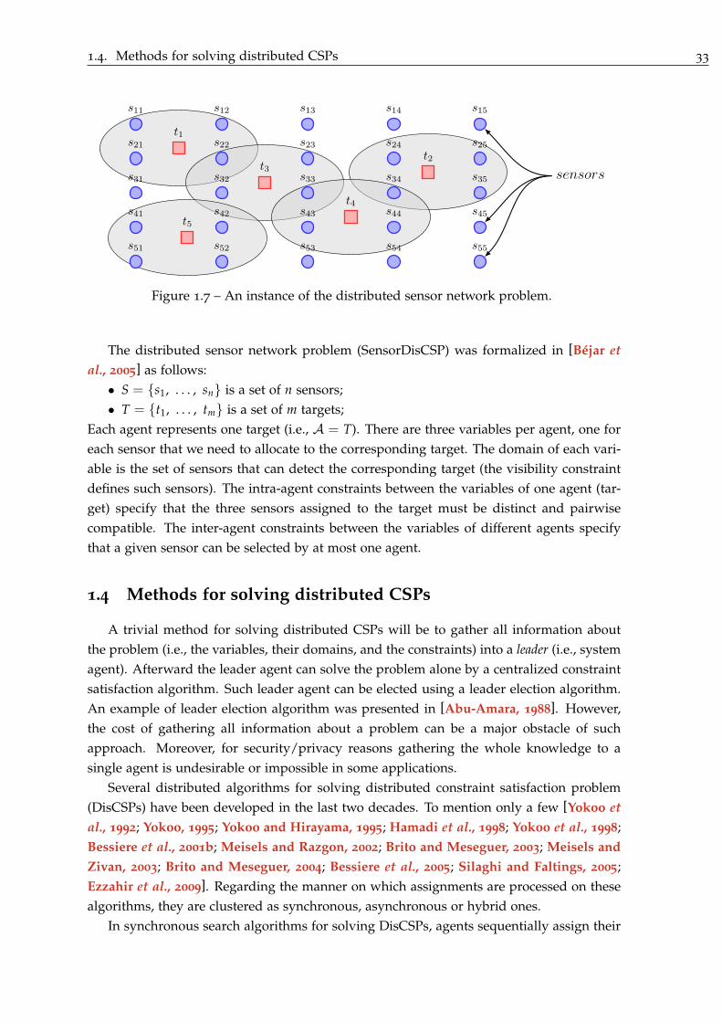
1.4. Methods for solving distributed CSPs 33
t1
t2t3
t4
t5
s11
s21
s31
s41
s51
s12
s22
s32
s42
s52
s13
s23
s33
s43
s53
s14
s24
s34
s44
s54
s15
s25
s35
s45
s55
sensors
Figure 1.7 – An instance of the distributed sensor network problem.
The distributed sensor network problem (SensorDisCSP) was formalized in [Béjar et
al., 2005] as follows:
• S = {s1, . . . , sn} is a set of n sensors;
• T = {t1, . . . , tm} is a set of m targets;
Each agent represents one target (i.e., A = T). There are three variables per agent, one for
each sensor that we need to allocate to the corresponding target. The domain of each vari-
able is the set of sensors that can detect the corresponding target (the visibility constraint
defines such sensors). The intra-agent constraints between the variables of one agent (tar-
get) specify that the three sensors assigned to the target must be distinct and pairwise
compatible. The inter-agent constraints between the variables of different agents specify
that a given sensor can be selected by at most one agent.
1.4 Methods for solving distributed CSPs
A trivial method for solving distributed CSPs will be to gather all information about
the problem (i.e., the variables, their domains, and the constraints) into a leader (i.e., system
agent). Afterward the leader agent can solve the problem alone by a centralized constraint
satisfaction algorithm. Such leader agent can be elected using a leader election algorithm.
An example of leader election algorithm was presented in [Abu-Amara, 1988]. However,
the cost of gathering all information about a problem can be a major obstacle of such
approach. Moreover, for security/privacy reasons gathering the whole knowledge to a
single agent is undesirable or impossible in some applications.
Several distributed algorithms for solving distributed constraint satisfaction problem
(DisCSPs) have been developed in the last two decades. To mention only a few [Yokoo et
al., 1992; Yokoo, 1995; Yokoo and Hirayama, 1995; Hamadi et al., 1998; Yokoo et al., 1998;
Bessiere et al., 2001b; Meisels and Razgon, 2002; Brito and Meseguer, 2003; Meisels and
Zivan, 2003; Brito and Meseguer, 2004; Bessiere et al., 2005; Silaghi and Faltings, 2005;
Ezzahir et al., 2009]. Regarding the manner on which assignments are processed on these
algorithms, they are clustered as synchronous, asynchronous or hybrid ones.
In synchronous search algorithms for solving DisCSPs, agents sequentially assign their

34 Chapter 1. Background
variables. Synchronous algorithms are based on notion of token, that is, the privileged of
assigning the variable. The token is passed among agents in synchronous algorithms and
then only the agent holding the token is activated while the rest of agents are waiting. Thus,
agents perform the assignment of their variable only when they hold a token. Although
synchronous algorithms do not exploit the parallelism inherent from the distributed sys-
tem, their agents receive consistent information from each other.
In the asynchronous search algorithms, agents act concurrently and asynchronously
without any global control. Hence, all agents are activated an then have the privileged
of assigning their variables asynchronously. Asynchronous algorithms are executed au-
tonomously by each agent in the distributed problem where agents do not need to wait
for decisions of other agents. Thus, agents take advantage from the distributed formalism
to enhance the degree of parallelism. However, in asynchronous algorithms, the global
assignment state at any particular agent is in general inconsistent.
1.4.1 Synchronous search algorithms on DisCSPs
Synchronous Backtracking (SBT) is the simplest search algorithm for solving DisCSPs[Yokoo, 2000b]. SBT is a straightforward extension of the chronological Backtracking al-
gorithm for centralized CSPs (Section 1.2.1.1). SBT requires a total order on which agents
will be instantiated. Following this ordering, agents perform assignments sequentially and
synchronously. When an agent receives a partial solution from its predecessor, it assigns
its variable a value satisfying constraints it knows. If it succeeds in finding such value, it
extends the partial solution by adding its assignment on it and passes it on to its successor.
When no value is possible for its variable, then it sends a backtracking message to its pre-
decessor. In SBT, only the agent holding the current partial assignment (CPA) performs an
assignment or backtrack.
Zivan and Meisels (2003) proposed the Synchronous Conflict-Based Backjumping (SCBJ),
a distributed version of the centralized (CBJ) algorithm [Prosser, 1993], see Section 1.2.1.2.
While SBT performs chronological backtracking, SCBJ performs backjumping. Each agent
Ai keep the conflict set (CSi). When a wipe-out occurs on its domain, a jump is performed
to the closest conflict variable in CSi. The backjumping message will contain CSi. When an
agent receives a backjumping message, it discards it current value, and updates its conflict
set to be the union of its old conflict-set and the one received.
Extending SBT, Meisels and Zivan (2007) proposed the Asynchronous Forward-
Checking (AFC). Besides assigning variables sequentially as is done in SBT, agents in AFC
perform forward checking (FC [Haralick and Elliott, 1980]) asynchronously. The key here
is that each time an agent succeeds to extend the current partial assignment (by assigning
its variable), it sends the CPA to its successor and copies of this CPA to all agents whose
assignments are not yet on the CPA. When an agent receives a copy of the CPA, it performs
the forward checking phase. In the forward checking phase all inconsistent values with
assignments on the received CPA are removed. The forward checking operation is per-
formed asynchronously where comes the name of the algorithm. When an agent generates
an empty domain as a result of a forward checking, it informs all agents with unassigned

1.4. Methods for solving distributed CSPs 35
variables on the (inconsistent) CPA. Afterwards, one of these agents will receive the CPA
and will backtrack. Thereby, only one backtrack can be generated for a given CPA.
1.4.1.1 Asynchronous Forward-Checking (AFC)
The Asynchronous Forward-Checking (AFC) is a synchronous search algorithm that
processes only consistent partial assignments. These assignments are processed syn-
chronously. In AFC algorithm, the state of the search process is represented by a data
structure called Current Partial Assignment (CPA).
Definition 1.22 A current partial assignment, CPA, is an ordered set of assignments
{[(x1, v1, t1), . . . , (xi, vi, ti)] | x1 ≺ · · · ≺ xi}. Two CPAs are compatible if every common
variable is assigned the same value in both CPAs.
Each CPA is associated with a counter that is updated by each agent when it succeeds
in assigning its variable on the CPA. This counter, called Step-Counter (SC), acts as a time-
stamp for the CPA. In AFC algorithm, each agent stores the current assignments state of its
higher priority agents on the AgentView. The AgentView of an agent Ai ∈ A has a form
similar to a CPA. The AgentView contains a consistency flag, AgentView.Consistent, that
represents whether the partial assignment it holds is consistent. The pseudo-code of AFC
algorithm executed by a generic agent Ai is shown in Algorithm 1.5.
Agent Ai starts the search by calling procedure AFC() in which it initializes counters to
0. Next, if Ai is the initializing agent IA (the first agent in the agent ordering, O), it initiates
the search by calling procedure Assign() (line 2). Then, a loop considers the reception and
the processing of the possible message types. Thus, agents wait for messages, and then call
the procedures dealing with the relevant type of message received.
When calling procedure Assign() Ai tries to find an assignment, which is consis-
tent with its AgentView. If Ai fails to find a consistent assignment, it calls procedure
Backtrack() (line 13). If Ai succeeds, it generates a CPA from its AgentView augmented
by its assignment, increments the Step Counter SC (lines 10-11), and then calls procedure
SendCPA(CPA) (line 12). If the CPA includes all agents assignments (Ai is the lowest agent
in the ordering, line 14), Ai reports the CPA as a solution of the problem and marks the
end flag true to stop the main loop (line 15). Otherwise, Ai sends forward the CPA to every
agent whose assignments are not yet on the CPA (line 17). Next agent on the ordering (suc-
cessor, Ai+1) will receive the CPA in a cpa message and then will try to extend this CPA by
assigning its variable on it (line 17). Other unassigned agents will receive the CPA, gener-
ated by Ai, in fc_cpa (line 18). Therefore, these agents will perform the forward-checking
phase asynchronously to check its consistency.
Ai calls procedure Backtrack() when it is holding the CPA in one of two cases. Ei-
ther Ai can not find a consistent assignment for its variable (line 13), or its AgentView is
inconsistent and is found to be compatible with the received CPA (line 30). If Ai is the
initializing agent IA, line 19, this means that the problem is unsolvable. Ai ends then the
search by marking the end flag true to stop the main loop and sending a stp message to all
agent informing them that search ends unsuccessfully (line 19). Other agents performing a

36 Chapter 1. Background
Algorithm 1.5: The AFC algorithm running by agent Ai.procedure AFC()
01. vi ← empty; ti ← 0; SC ← 0; end ← false; AgentView.Consistent ← true;02. if ( Ai = IA ) then Assign();03. while ( ¬end ) do04. msg ← getMsg();05. switch ( msg.type ) do06. cpa : ProcessCPA(msg); fc_cpa : ProcessFCCPA(msg.CPA);07. back_cpa : ProcessCPA(msg); not_ok : ProcessNotOk(msg.CPA);08. stp : end ← true;
procedure Assign()
09. if ( D(xi) �= ∅ ) then10. vi ← ChooseValue(); ti ← ti + 1 ;11. CPA ← {AgentView ∪ myAssig}; CPA.SC ← AgentView.SC + 1 ;12. SendCPA(CPA) ;13. else Backtrack();procedure SendCPA(CPA)14. if ( Ai is the last agent in O ) then15. end ← true; broadcastMsg : stp(CPA)16. else17. sendMsg : cpa(CPA) to Ai+1 ; /* Ai+1 is the agent next Ai */18. foreach ( Ak � Ai+1 ) do sendMsg : fc_cpa(CPA) to Ak ;
procedure Backtrack()
19. if ( Ai = IA ) then end ← true; broadcastMsg : stp() ;20. else21. AgentView ← shortest inconsistent partial assignment ;22. AgentView.Consistent ← false;23. sendMsg : back_cpa(AgentView) to Aj ; /* Aj denotes the last agent on AgentView */
procedure ProcessCPA(msg)24. CheckConsistencyOfAgentView(msg.CPA) ;25. if ( AgentView.Consistent ) then26. if ( msg.Sender � xi ) then store msg.CPA as justification of vi removal ;27. else UpdateAgentView(msg.CPA) ;28. Assign() ;
procedure CheckConsistencyOfAgentView(CPA)29. if ( ¬AgentView.Consistent ) then30. if ( AgentView ⊆ CPA ) then Backtrack() ;31. else AgentView.Consistent ← true ;
procedure UpdateAgentView(CPA)32. AgentView ← CPA; AgentView.SC ← CPA.SC ;33. foreach ( v ∈ D(xi) such that ¬isConsistent(v, CPA ) ) do34. store the shortest inconsistent partial assignment as justification of v removal;procedure ProcessFCCPA(CPA)35. if ( CPA.SC > AgentView.SC ) then36. if ( ¬AgentView.Consistent ) then37. if ( ¬AgentView ⊆ CPA ) then AgentView.Consistent ← true ;38. if ( AgentView.Consistent ) then39. UpdateAgentView(CPA) ;40. if ( D(xi) = ∅ ) then41. sendMsg : not_ok(CPA) to unassigned agents on AgentView ;
procedure ProcessNotOk(CPA)42. if ( CPA ⊆ AgentView ∨ (AgentView � CPA ∧ CPA.SC > AgentView.SC) ) then43. AgentView ← msg.CPA ;44. AgentView.Consistent ← false ;
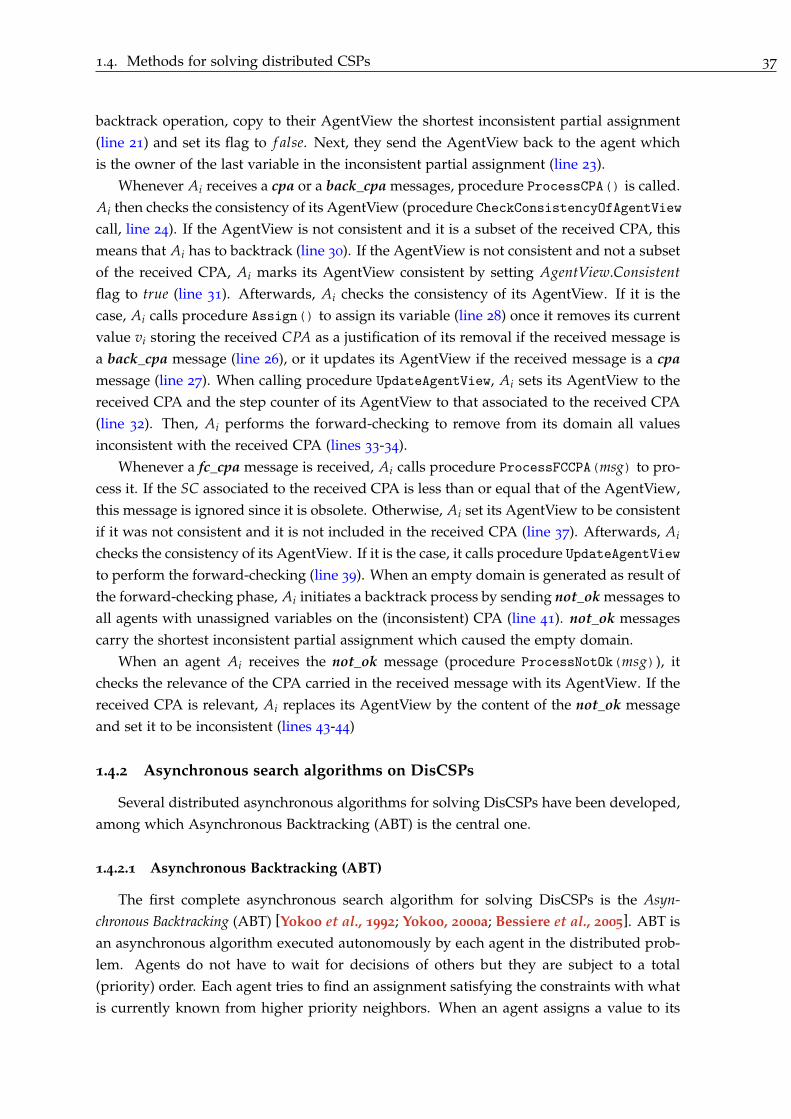
1.4. Methods for solving distributed CSPs 37
backtrack operation, copy to their AgentView the shortest inconsistent partial assignment
(line 21) and set its flag to f alse. Next, they send the AgentView back to the agent which
is the owner of the last variable in the inconsistent partial assignment (line 23).
Whenever Ai receives a cpa or a back_cpa messages, procedure ProcessCPA() is called.
Ai then checks the consistency of its AgentView (procedure CheckConsistencyOfAgentView
call, line 24). If the AgentView is not consistent and it is a subset of the received CPA, this
means that Ai has to backtrack (line 30). If the AgentView is not consistent and not a subset
of the received CPA, Ai marks its AgentView consistent by setting AgentView.Consistent
flag to true (line 31). Afterwards, Ai checks the consistency of its AgentView. If it is the
case, Ai calls procedure Assign() to assign its variable (line 28) once it removes its current
value vi storing the received CPA as a justification of its removal if the received message is
a back_cpa message (line 26), or it updates its AgentView if the received message is a cpa
message (line 27). When calling procedure UpdateAgentView, Ai sets its AgentView to the
received CPA and the step counter of its AgentView to that associated to the received CPA
(line 32). Then, Ai performs the forward-checking to remove from its domain all values
inconsistent with the received CPA (lines 33-34).
Whenever a fc_cpa message is received, Ai calls procedure ProcessFCCPA(msg) to pro-
cess it. If the SC associated to the received CPA is less than or equal that of the AgentView,
this message is ignored since it is obsolete. Otherwise, Ai set its AgentView to be consistent
if it was not consistent and it is not included in the received CPA (line 37). Afterwards, Ai
checks the consistency of its AgentView. If it is the case, it calls procedure UpdateAgentView
to perform the forward-checking (line 39). When an empty domain is generated as result of
the forward-checking phase, Ai initiates a backtrack process by sending not_ok messages to
all agents with unassigned variables on the (inconsistent) CPA (line 41). not_ok messages
carry the shortest inconsistent partial assignment which caused the empty domain.
When an agent Ai receives the not_ok message (procedure ProcessNotOk(msg)), it
checks the relevance of the CPA carried in the received message with its AgentView. If the
received CPA is relevant, Ai replaces its AgentView by the content of the not_ok message
and set it to be inconsistent (lines 43-44)
1.4.2 Asynchronous search algorithms on DisCSPs
Several distributed asynchronous algorithms for solving DisCSPs have been developed,
among which Asynchronous Backtracking (ABT) is the central one.
1.4.2.1 Asynchronous Backtracking (ABT)
The first complete asynchronous search algorithm for solving DisCSPs is the Asyn-
chronous Backtracking (ABT) [Yokoo et al., 1992; Yokoo, 2000a; Bessiere et al., 2005]. ABT is
an asynchronous algorithm executed autonomously by each agent in the distributed prob-
lem. Agents do not have to wait for decisions of others but they are subject to a total
(priority) order. Each agent tries to find an assignment satisfying the constraints with what
is currently known from higher priority neighbors. When an agent assigns a value to its

38 Chapter 1. Background
variable, the selected value is sent to lower priority neighbors. When no value is possi-
ble for a variable, the inconsistency is reported to higher agents in the form of a nogood
(see Definition 1.13). ABT computes a solution (or detects that no solution exists) in a finite
time. To be complete, ABT requires a total ordering on agents. The total ordering on agents
is static.
The required total ordering on agents in ABT provides a directed acyclic graph. Con-
straints are then directed according to the total order among agents. Hence, a directed
link between each two constrained agents is established. ABT uses this structure between
agent to perform the asynchronous search. Thus, the agent from which a link departs is
the value-sending agent and the agent to which the link arrives is the constraint-evaluating
agent. The pseudo-code executed by a generic agent Ai ∈ A is presented in Algorithm 1.6.
In ABT, each agent keeps some amount of local information about the global search,
namely an AgentView and a NogoodStore. A generic agent, say Ai, stores in its AgentView
the most up to date values that it believes are assigned to its higher priority neighbors.
Ai stores in its NogoodStore nogoods justifying values removal. Agents exchange the
following types of messages (where Ai is the sender):
ok?: Ai informs a lower priority neighbor about its assignment.
ngd: Ai informs a higher priority neighbor of a new nogood.
adl: Ai requests a higher priority agent to set up a link.
stp: The problem is unsolvable because an empty nogood has been generated.
In the main procedure ABT(), each agent selects a value and informs other agents
(CheckAgentView call, line 2). Then, a loop receives and processes messages (line 3-7).
CheckAgentView checks if the current value (vi) is consistent with AgentView. If vi is
inconsistent with assignments of higher priority neighbors, Ai tries to select a consistent
value (ChooseValue call, line 9). In this process, some values from D(xi) may appear as
inconsistent. Thus, nogoods justifying their removal are added to the NogoodStore of Ai
(line 39). When two nogoods are possible for the same value, Ai selects the best with the
Highest Possible Lowest Variable heuristic [Hirayama and Yokoo, 2000; Bessiere et al., 2005].
If a consistent value exist, it is returned and then assigned to xi. Then, Ai notifies its new
assignment to all agents in Γ+(xi) through ok? messages (line 11). Otherwise, Ai has to
backtrack (procedure Backtrack() call, line 12).
Whenever it receives an ok? message, Ai processes it by calling procedure
ProcessInfo(msg). The AgentView of Ai is updated (UpdateAgentView call, line 13) only
if the received message contains an assignment more up to date than that already stored
for the sender (line 16) and all nogoods becomes non compatible with the AgentView of
Ai are removed (line 18). Then, a consistent value for Ai is searched after the change in the
AgentView (CheckAgentView call, line 14).
When every value of Ai is forbidden by its NogoodStore, procedure Backtrack()
is called. In procedure Backtrack(), Ai resolves its nogoods, deriving a new nogood,
newNogood (line 19). If newNogood is empty, the problem has no solution. Ai broadcasts
the stp messages to all agents and terminates the execution (line 20). Otherwise, the new
nogood is sent in a ngd message to the agent, say Aj, owning the variable appearing in its
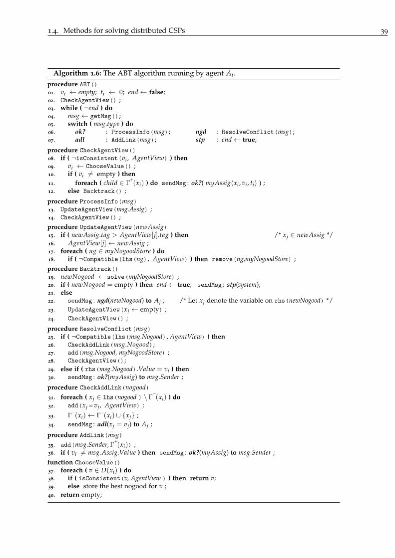
1.4. Methods for solving distributed CSPs 39
Algorithm 1.6: The ABT algorithm running by agent Ai.procedure ABT()
01. vi ← empty; ti ← 0; end ← false;02. CheckAgentView() ;03. while ( ¬end ) do04. msg ← getMsg();05. switch ( msg.type ) do06. ok? : ProcessInfo(msg); ngd : ResolveConflict(msg);07. adl : AddLink(msg); stp : end ← true;
procedure CheckAgentView()
08. if ( ¬isConsistent(vi , AgentView) ) then09. vi ← ChooseValue() ;10. if ( vi �= empty ) then
11. foreach ( child ∈ Γ+(xi) ) do sendMsg : ok?( myAssig�xi , vi , ti� ) ;
12. else Backtrack() ;
procedure ProcessInfo(msg)13. UpdateAgentView(msg.Assig) ;14. CheckAgentView() ;procedure UpdateAgentView(newAssig)15. if ( newAssig.tag > AgentView[j].tag ) then /* xj ∈ newAssig */16. AgentView[j] ← newAssig ;17. foreach ( ng ∈ myNogoodStore ) do18. if ( ¬Compatible(lhs(ng), AgentView) ) then remove(ng,myNogoodStore) ;procedure Backtrack()
19. newNogood ← solve(myNogoodStore) ;20. if ( newNogood = empty ) then end ← true; sendMsg : stp(system);21. else22. sendMsg : ngd(newNogood) to Aj ; /* Let xj denote the variable on rhs(newNogood) */23. UpdateAgentView(xj ← empty) ;24. CheckAgentView() ;
procedure ResolveConflict(msg)25. if ( ¬Compatible(lhs(msg.Nogood), AgentView) ) then26. CheckAddLink(msg.Nogood);27. add(msg.Nogood, myNogoodStore) ;28. CheckAgentView();29. else if ( rhs(msg.Nogood).Value = vi ) then30. sendMsg : ok?(myAssig) to msg.Sender ;
procedure CheckAddLink(nogood)
31. foreach ( xj ∈ lhs(nogood ) \ Γ−(xi) ) do
32. add(xj = vj, AgentView) ;
33. Γ−(xi) ← Γ
−(xi) ∪ {xj} ;
34. sendMsg : adl(xj = vj) to Aj ;
procedure AddLink(msg)
35. add(msg.Sender,Γ+(xi)) ;
36. if ( vi �= msg.Assig.Value ) then sendMsg : ok?(myAssig) to msg.Sender ;function ChooseValue()
37. foreach ( v ∈ D(xi) ) do38. if ( isConsistent(v, AgentView ) ) then return v;39. else store the best nogood for v ;40. return empty;

40 Chapter 1. Background
rhs (line 22). Then, the assignment of xj is deleted from the AgentView (UpdateAgentView
call, line 23). Finally, a new consistent value is selected (CheckAgentView call, line 24).
Whenever Ai receives a ngd message, procedure ResolveConflict is called. The no-
good included in the ngd message is accepted only if its lhs is compatible with assignments
on the AgentView of Ai. Next, Ai calls procedure CheckAddLink (line 26). In procedure,
CheckAddLink() the assignments in the received nogood for variables not directly linked
with Ai are taken to update the AgentView (line 32) and a request for a new link is sent to
agents owning these variables (line 34). Next, the nogood is stored, acting as justification
for removing the value on its rhs (line 27). A new consistent value for Ai is then searched
(CheckAgentView call, line 28) if the current value was removed by the received nogood.
If the nogood is not compatible with the AgentView, it is discarded since it is obsolete.
However, if the value of xi was correct in the received nogood, Ai re-sends its assignment
to the nogood sender by an ok? message (lines 29-30).
When a link request is received, Ai calls procedure AddLink(msg). Then, the sender is
included in Γ+(xi) (line 35). Afterwards, Ai sends its assignment through an ok? message
to the sender if its value is different than that included in the received msg (line 36).
In order to be complete, ABT in its original version may request adding links between
initially unrelated agents. Given the manner to how these links are set Bessiere et al.
proposed 4 version of ABT that have been all proven to be complete [Bessiere et al., 2005].
By the way, they rediscover already existent algorithms like ABT [Yokoo et al., 1998], or
DIBT [Hamadi et al., 1998].
ABT (Adding links during search): In ABT, presented above, new links between unrelated
agents may be added during search. A link is requested by an agent when it receives
a ngd message containing unrelated agents in the ordering. New links are permanent.
These links are used to remove obsolete information stored by a given agent.
ABTall (Adding links as preprocessing): In ABTall , all the potentially useful links are added
during a preprocessing step. New links are permanent.
ABTtemp(k) (Adding temporary links): In ABTtemp(k), unrelated agents may be requested to
add a link between them. However, the added links are temporary. This idea was
firstly introduced in [Silaghi et al., 2001d]. New links are kept only for a fixed
number of messages (k). Hence, each added link is removed after exchanging k
messages through it.
ABTnot (No links): ABTnot no more needs links to be complete. To achieve its completeness,
it has only to remove obsolete information in finite time. Thus, all nogoods that
hypothetically could become obsolete are forgotten after each backtrack.
Figure 1.8 illustrates an example of Asynchronous Backtracking algorithm execution
on a simple instance (Figure 1.8(a)). This instance includes three agents, each holding
one variable (x1, x2 and x3). There domains are respectively {1, 2}, {2} and {1, 2}. This
instance includes two constraints x1 �= x3 and x2 �= x3. In Figure 1.8(b), by receiving ok?
messages from x1 and x2, the AgentView of x3 will be [x1 = 1, x2 = 2]. These assignments
remove values 1 and 2 from D(x3) storing two nogoods as justification of there removal

1.4. Methods for solving distributed CSPs 41
x1 x2
x3
�= �=
D(x1)={1, 2} D(x2)={2}
D(x3)={1, 2}
(a)
x1 x2
x3
�= �=
D(x1)={1, 2} D(x2)={2}
D(x3)={1, 2}
ok?(x1 = 1) ok?(x2 = 2)
AgentV iew : [x1 = 1, x2 = 2]
x1 = 1 → x3 �= 1
x2 = 2 → x3 �= 2
(b)
x1 x2
x3
�= �=
D(x1)={1, 2} D(x2)={2}
D(x3)={1, 2}
AgentV iew : [x1 = 1]
x1 = 1 → x3 �= 1
x1 = 1 → x2 �= 2
ngd(x1 = 1 → x2 �= 2)
(c)
x1 x2
x3
�= �=
D(x1)={1, 2} D(x2)={2}
D(x3)={1, 2}
AgentV iew:[x1=1]
x1 = 1 → x3 �= 1
AgentV iew:[x1=1]
adl(x1 = 1)
x1=1 → x2 �= 2
(d)
x1 x2
x3
�= �=
D(x1)={1, 2} D(x2)={2}
D(x3)={1, 2}
AgentV iew : [x1 = 1]
x1 = 1 → x3 �= 1
ngd([] → x1 �= 1)[]→x1 �=1
(e)
x1 x2
x3
�= �=
D(x1)={1, 2} D(x2)={2}
D(x3)={1, 2}
[] → x1 �= 1
ok?(x2 = 2)
ok?(x1 = 2)
ok?(x1=2)
AgentV iew:[x1=2]
AgentV iew:[x1=2, x2=2]
(f)
Figure 1.8 – An example of Asynchronous Backtracking execution.
(i.e., x1=1 → x3 �= 1 respectively, x2=2 → x3 �= 2). Since there is no possible value
consistent with its AgentView, agent x3 resolves its nogoods producing a new nogood
(x1=1 → x2 �= 2) (Figure 1.8(c)). This nogood is then sent to x2 in ngd message. By receiving
this ngd message, agent x2 records this nogood. This nogood contains assignment of agent
x1, which is not connected to x2 by a link. Therefore, agent x2 requests a new link between
him and x1 by sending an adl message (Figure 1.8(d)). Agent x2 checks whether its value
is consistent with its AgentView ([x1 = 1]). Since its only value 2 is removed by the nogood
received from x3, agent x2 resolves its NogoodStore producing a new nogood, [] → x1 �= 1.
This nogood is then sent to agent x1 (Figure 1.8(e)). This nogood will lead x1 to change its
current value to 1, and henceforth it will send its assignment on an ok? message to both

42 Chapter 1. Background
agent x2 and x3. Simultaneously, agent x2 assigns its variable and then sends its assignment
to its lower priority neighbor x3. Hence, we get the situation shown in Figure 1.8(f).
1.4.3 Dynamic Ordering Heuristics on DisCSPs
In algorithms presented above for solving DisCSPs, the total ordering on agents is static.
Therefore, a single mistake on the order is very penalizing. Moreover, it is known from
centralized CSPs that dynamic reordering of variables during search drastically fastens the
search procedure (see Section 1.2.2.2). Many attempts were made to apply this principle
for improving distributed constraint algorithms.
The first reordering algorithm for DisCSP is the Asynchronous Weak Commitment
(AWC) [Yokoo, 1995]. Asynchronous Weak Commitment (AWC) dynamically reorders
agents during search by moving the sender of a nogood higher in the order than the other
agents in the nogood. Whenever a wipe-out occurs on the domain of a variable xi, the total
agent ordering is revised so as to assign the highest priority to the agent xi. While AWC
was shown to outperform ABT empirically on small problems, contrary to ABT, the AWC
algorithm requires an exponential space for storing all generated nogoods.
Silaghi et al. (2001c) later proposed Asynchronous Backtracking with Reordering
(ABTR) an attempt to hybridize ABT with AWC. Abstract agents fulfill the reordering
operation to guarantee a finite number of asynchronous reordering operations. Asyn-
chronous Backtracking with Reordering is the first asynchronous complete algorithm with
polynomial space requirements that enables a largest number of reordering heuristics in
asynchronous search. However, to achieve this the position of first agent on the ordering
had to be fix. A dynamic variable reordering heuristic for ABTR that exactly mimics the
one employed in centralized Dynamic Backtracking [Ginsberg, 1993] and that requires no
exchange of heuristic messages was presented in [Silaghi, 2006].
Zivan and Meisels (2006a) proposed Dynamic Ordering for Asynchronous Backtrack-
ing (ABT_DO aka ABTR). ABT_DO is a simple algorithm for dynamic ordering in Asyn-
chronous Backtracking search. Agents choose orders dynamically and asynchronously
while keeping space complexity polynomial. When an ABT_DO agent changes its assign-
ment, it can reorder all agents with lower priority. Zivan and Meisels proposed three dif-
ferent ordering heuristics in ABT_DO. In the best of those heuristics called Nogood-triggered
heuristic, inspired by dynamic backtracking [Ginsberg, 1993], the agent that generates a
nogood is placed in front of all other lower priority agents.
A new kind of ordering heuristics for ABT_DO is presented in [Zivan et al., 2009].
These heuristics, called retroactive heuristics, enable the generator of the nogood to be
moved to a higher position than that of the target of the backtrack. The degree of flexibility
of these retroactive heuristics depends on a parameter K. K defines the level of flexibility of
the heuristic with respect to the amount of information an agent can store in its memory.
Agents that detect a dead end move themselves to a higher priority position in the order.
If the length of the nogood generated is not larger than K then the agent can move to any
position it desires (even to the highest priority position) and all agents that are included in
the nogood are required to add the nogood to their set of constraints and hold it until the

1.5. Summary 43
algorithm terminates. Since agents must store nogoods that are smaller than or equal to
K, the space complexity of agents is exponential in K. If the size of the created nogood is
larger than K, the agent that generated the nogood can move up to the place that is right
after the second last agent in the nogood.
The best retroactive heuristic introduced in [Zivan et al., 2009] is called ABT_DO-Retro-
MinDom. This heuristic does not require any additional storage (i.e., K = 0). In this
heuristic, the agent that generates a nogood is placed in the new order between the last
and the second last agents in the generated nogood. However, the generator of the nogood
moves to a higher priority position than the backtracking target (the agent the nogood
was sent to) only if its domain is smaller than that of the agents it passes on the way up.
Otherwise, the generator of the nogood is placed right after the last agent with a smaller
domain between the last and the second last agents in the nogood.
1.4.4 Maintaining Arc Consistency on DisCSPs
Although, its success for solving centralized CSPs was empirically demonstrated, the
Maintenance of Arc Consistency (MAC) has not yet been well investigated in distributed
CSPs. Silaghi et al. (2001b) introduced the Distributed Maintaining Asynchronously Con-
sistency for ABT, DMAC-ABT, the first algorithm able to maintain arc consistency in dis-
tributed CSPs [Silaghi et al., 2001b]. DMAC-ABT considers consistency maintenance as
a hierarchical nogood-based inference. However, the improvement obtained on ABT was
minor.
Brito and Meseguer (2008) proposed ABT-uac and ABT-dac, two algorithms that con-
nect ABT with arc consistency [Brito and Meseguer, 2008]. The first algorithm they pro-
pose, ABT-uac, propagates unconditionally deleted values (i.e., values removed by a no-
good having an empty left-hand side) to enforce an amount of full arc consistency. The
intuitive idea behind ABT-uac is since unconditionally deleted values are removed once
and for all, their propagation may causes new deletions in the domains of other variables.
Thus, the search effort required to solve the DisCSP can be reduced. The second algo-
rithm they propose, ABT-dac, extends the first one in order to propagate conditionally and
unconditionally deleted values using directional arc consistency. ABT-uac shows minor
improvement in communication load and ABT-dac is harmful in many instances.
1.5 Summary
We have described in this chapter the basic issues of centralized constraint satisfac-
tion problems (CSPs). After defining the constraint satisfaction problem formalism (CSP)
and presenting some examples of academical and real combinatorial problems that can be
modeled as CSP, we reported the main existent algorithms and heuristics used for solving
centralized constraint satisfaction problems. Next, we formally define the distributed con-
straint satisfaction problem (DisCSP) paradigm. Some examples of real world applications
have been presented and then encoded in DisCSP. Finally, we provide the state of the art
methods for solving DisCSPs.

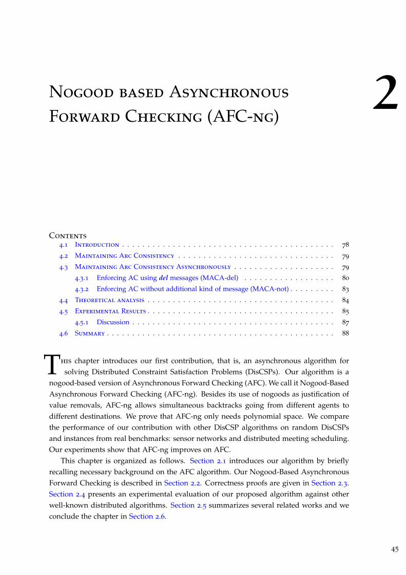
2Nogood based Asynchronous
Forward Checking (AFC-ng)
Contents4.1 Introduction . . . . . . . . . . . . . . . . . . . . . . . . . . . . . . . . . . . . . . . . . . 78
4.2 Maintaining Arc Consistency . . . . . . . . . . . . . . . . . . . . . . . . . . . . . . . 79
4.3 Maintaining Arc Consistency Asynchronously . . . . . . . . . . . . . . . . . . . . 79
4.3.1 Enforcing AC using del messages (MACA-del) . . . . . . . . . . . . . . . . . . 80
4.3.2 Enforcing AC without additional kind of message (MACA-not) . . . . . . . . . 83
4.4 Theoretical analysis . . . . . . . . . . . . . . . . . . . . . . . . . . . . . . . . . . . . . 84
4.5 Experimental Results . . . . . . . . . . . . . . . . . . . . . . . . . . . . . . . . . . . . . 85
4.5.1 Discussion . . . . . . . . . . . . . . . . . . . . . . . . . . . . . . . . . . . . . . . . 87
4.6 Summary . . . . . . . . . . . . . . . . . . . . . . . . . . . . . . . . . . . . . . . . . . . . . 88
This chapter introduces our first contribution, that is, an asynchronous algorithm for
solving Distributed Constraint Satisfaction Problems (DisCSPs). Our algorithm is a
nogood-based version of Asynchronous Forward Checking (AFC). We call it Nogood-Based
Asynchronous Forward Checking (AFC-ng). Besides its use of nogoods as justification of
value removals, AFC-ng allows simultaneous backtracks going from different agents to
different destinations. We prove that AFC-ng only needs polynomial space. We compare
the performance of our contribution with other DisCSP algorithms on random DisCSPs
and instances from real benchmarks: sensor networks and distributed meeting scheduling.
Our experiments show that AFC-ng improves on AFC.
This chapter is organized as follows. Section 2.1 introduces our algorithm by briefly
recalling necessary background on the AFC algorithm. Our Nogood-Based Asynchronous
Forward Checking is described in Section 2.2. Correctness proofs are given in Section 2.3.
Section 2.4 presents an experimental evaluation of our proposed algorithm against other
well-known distributed algorithms. Section 2.5 summarizes several related works and we
conclude the chapter in Section 2.6.
45

46 Chapter 2. Nogood based Asynchronous Forward Checking (AFC-ng)
2.1 Introduction
As seen in Section 1.4.1 Asynchronous Forward-Checking (AFC) incorporates the idea
of the forward-checking (FC) algorithm for centralized CSP [Haralick and Elliott, 1980].
However, agents perform the forward checking phase asynchronously [Meisels and Zi-
van, 2003; Meisels and Zivan, 2007]. As in synchronous backtracking, agents assign their
variables only when they hold the current partial assignment (cpa). The cpa is a unique
message (token) that is passed from one agent to the next one in the ordering. The cpa
message carries the partial assignment (CPA) that agents attempt to extend into a complete
solution by assigning their variables on it. When an agent succeeds in assigning its vari-
able on the CPA, it sends this CPA to its successor. Furthermore, copies of the CPA are
sent to all agents whose assignments are not yet on the CPA. These agents perform the
forward checking asynchronously in order to detect as early as possible inconsistent par-
tial assignments. The forward-checking process is performed as follows. When an agent
receives a CPA, it updates the domain of its variable, removing all values that are in con-
flict with assignments on the received CPA. Furthermore, the shortest CPA producing the
inconsistency is stored as justification of the value deletion.
When an agent generates an empty domain as a result of a forward-checking, it initi-
ates a backtrack process by sending not_ok messages. not_ok messages carry the shortest
inconsistent partial assignment which caused the empty domain. not_ok messages are sent
to all agents with unassigned variables on the (inconsistent) CPA. When an agent receives
the not_ok message, it checks if the CPA carried in the received message is compatible
with its AgentView. If it is the case, the receiver stores the not_ok, otherwise, the not_ok
is discarded. When an agent holding a not_ok receives a CPA on a cpa message from its
predecessor, it sends this CPA back in a back_cpa message. When multiple agents reject
a given assignment by sending not_ok messages, only the first agent that will receive a
cpa message from its predecessor and is holding a relevant not_ok message will eventually
backtrack. After receiving a new cpa message, the not_ok message becomes obsolete when
the CPA it carries is no longer a subset of the received CPA.
The manner in which the backtrack operation is performed is a major drawback of
the AFC algorithm. The backtrack operation requires a lot of work from the agents. An
improved backtrack method for AFC was described in Section 6 of [Meisels and Zivan,
2007]. Instead of just sending not_ok messages to all agents unassigned in the CPA, the
agent who detects the empty domain can itself initiate a backtrack operation. It sends a
backtrack message to the last agent assigned in the inconsistent CPA in addition to the
not_ok messages to all agents not instantiated in the inconsistent CPA. The agent who
receives a backtrack message generates (if it is possible) a new CPA that will dominate
older ones thanks to a time-stamping mechanism.
We present in this chapter the Nogood-based Asynchronous Forward Checking (AFC-
ng), an algorithm for solving DisCSPs based on Asynchronous Forward Checking (AFC).
Instead of using the shortest inconsistent partial assignments we use nogoods as justifica-
tions of value removals. Unlike AFC, AFC-ng allows concurrent backtracks to be performed
at the same time coming from different agents having an empty domain to different des-

2.2. Nogood-based Asynchronous Forward Checking 47
tinations. As a result, several CPAs could be generated simultaneously by the destination
agents. Thanks to the timestamps integrated in the CPAs, the strongest CPA coming from
the highest level in the agent ordering will eventually dominate all others. Interestingly, the
search process with the strongest CPA will benefit from the computational effort done by
the (killed) lower level processes. This is done by taking advantage from nogoods recorded
when processing these lower level processes.
2.2 Nogood-based Asynchronous Forward Checking
The nogood-based Asynchronous Forward-Checking (AFC-ng) is based on the Asyn-
chronous Forward Checking (AFC). AFC-ng tries to enhance the asynchronism of the for-
ward checking phase. The two main features of AFC-ng are the following. First, it uses the
nogoods as justification of value deletions. Each time an agent performs a forward-check, it
revises its initial domain, (including values already removed by a stored nogood) in order to
store the best nogoods for removed values (one nogood per value). When comparing two
nogoods eliminating the same value, the nogood with the Highest Possible Lowest Variable
involved is selected (HPLV heuristic) [Hirayama and Yokoo, 2000]. As a result, when an
empty domain is found, the resolvent nogood contains variables as high as possible in the
ordering, so that the backtrack message is sent as high as possible, thus saving unnecessary
search effort [Bessiere et al., 2005].
Second, each time an agent Ai generates an empty domain it no longer sends not_ok
messages. It resolves the nogoods ruling out values from its domain, producing a new
nogood newNogood. newNogood is the conjunction of the left hand sides of all nogoods
stored by Ai. Then, Ai sends the resolved nogood newNogood in a ngd (backtrack) message
to the lowest agent in newNogood. Hence, multiple backtracks may be performed at the
same time coming from different agents having an empty domain. These backtracks are
sent concurrently by these different agents to different destinations. The reassignment of
the destination agents then happen simultaneously and generate several CPAs. However,
the strongest CPA coming from the highest level in the agent ordering will eventually
dominate all others. Agents use the timestamp (see Definition 2.1) to detect the strongest
CPA. Interestingly, the search process of higher levels with stronger CPAs can use nogoods
reported by the (killed) lower level processes, so that it benefits from their computational
effort.
2.2.1 Description of the algorithm
In the Asynchronous Forward-Checking only the agent holding the current partial as-
signment, CPA (Definition 1.22) can perform an assignment or backtracks. In order to
enhance the asynchronism of the forward-checking phase, unlike AFC, the nogood-based
Asynchronous Forward-Checking algorithm (AFC-ng) allows simultaneous backtracks go-
ing from different agents to different destinations. The reassignments of the destination
agents then happen simultaneously and generate several CPAs. For allowing agents to

48 Chapter 2. Nogood based Asynchronous Forward Checking (AFC-ng)
simultaneously propose new CPAs, they must be able to decide which CPA to select. We
propose that the priority between the CPAs is based on timestamp.
Definition 2.1 A timestamp associated with a CPA is an ordered list of counters [t1, t2, . . . , ti]
where tj is the tag of the variable xj. When comparing two CPAs, the strongest one is that associated
with the lexicographically greater timestamp. That is, the CPA with greatest value on the first
counter on which they differ, if any, otherwise the longest one.
Based on the timestamp associated with each CPA, now agents can detect the strongest
CPA. Therefore, the strongest CPA coming from the highest level in the agent ordering will
eventually dominate all others.
Each agent Ai ∈ A executes the pseudo-code shown in Algorithm 2.1. Each agent Ai
stores a nogood per removed value in the NogoodStore. The other values not ruled out
by a nogood form D(xi), the current domain of xi. Moreover, Ai keeps an AgentView that
stores the most up to date assignments received from higher priority agents in the agent
ordering. It has a form similar to a current partial assignment CPA (see, Definition 1.22)
and is initialized to the set of empty assignments {(xj, empty, 0) | xj ≺ xi}.
Agent Ai starts the search by calling procedure AFC-ng() in which it initializes its
AgentView (line 1) by setting counters to zero (line 9). The AgentView contains a consis-
tency flag that represents whether the partial assignment it holds is consistent. If Ai is the
initializing agent IA (the first agent in the agent ordering), it initiates the search by calling
procedure Assign() (line 2). Then, a loop considers the reception and the processing of
the possible message types (lines 3-8). In AFC-ng, agents exchange the following types of
messages (where Ai is the sender):
cpa Ai passes on the current partial assignment (CPA) to a lower priority agent. According
to its position on the ordering, the receiver will try to extend the CPA (when it is the
next agent on the ordering) or perform the forward-checking phase.
ngd Ai reports the inconsistency to a higher priority agent. The inconsistency is reported
by a nogood.
stp Ai informs agents either if a solution is found or the problem is unsolvable.
When calling Assign() Ai tries to find an assignment, which is consistent with its
AgentView. If Ai fails to find a consistent assignment, it calls procedure Backtrack()
(line 14). If Ai succeeds, it increments its counter ti and generates a CPA from its AgentView
augmented by its assignment (line 12). Afterwards, Ai calls procedure SendCPA(CPA)
(line 13). If the CPA includes all agents assignments (Ai is the lowest agent in the order,
line 15), Ai reports the CPA as a solution of the problem and marks the end flag true to
stop the main loop (line 16). Otherwise, Ai sends forward the CPA to every agent whose
assignments are not yet on the CPA (line 17). So, the next agent on the ordering (successor)
will try to extend this CPA by assigning its variable on it while other agents will perform
the forward-checking phase asynchronously to check its consistency.
Whenever Ai receives a cpa message, procedure ProcessCPA(msg) is called (line 6). Ai
checks its AgentView status. If it is not consistent and the AgentView is a subset of the
received CPA, this means that Ai has already backtracked, then Ai does nothing (line 18).

2.2. Nogood-based Asynchronous Forward Checking 49
Algorithm 2.1: Nogood-based AFC (AFC-ng) algorithm running by agent Ai.procedure AFC-ng()
01. end ← false; AgentView.Consistent ← true; InitAgentView();02. if ( Ai = IA ) then Assign() ;03. while ( ¬end ) do04. msg ← getMsg();05. switch ( msg.type ) do06. cpa : ProcessCPA(msg);07. ngd : ProcessNogood(msg);08. stp : end ← true; if ( msg.CPA �= ∅ ) then solution ← msg.CPA ;
procedure InitAgentView()
09. foreach ( xj ≺ xi ) do AgentView[j] ← {(xj, empty, 0)} ;
procedure Assign()
10. if ( D(xi) �= ∅ ) then11. vi ← ChooseValue() ; ti ← ti + 1 ;12. CPA ← {AgentView ∪ myAssig} ;13. SendCPA(CPA) ;14. else Backtrack();procedure SendCPA(CPA)15. if ( size(CPA ) = n ) then /* Ai is the last agent in O */16. broadcastMsg : stp(CPA) ; end ← true17. else foreach ( xk � xi ) do sendMsg : cpa(CPA) to Ak ;procedure ProcessCPA(msg)18. if ( ¬AgentView.Consistent ∧ AgentView ⊂ msg.CPA ) then return ;19. if ( msg.CPA is stronger than AgentView ) then20. UpdateAgentView(msg.CPA) ; AgentView.Consistent ←true;21. Revise();22. if ( D(xi) = ∅ ) then Backtrack() ;23. else CheckAssign(msg.Sender) ;
procedure CheckAssign(sender)24. if ( Ai−1 = sender ) then Assign() ; /* the sender is the predecessor of Ai */procedure Backtrack()
25. newNogood ← solve(myNogoodStore) ;26. if ( newNogood = empty ) then broadcastMsg : stp( ∅ ); end ← true;27. else28. sendMsg : ngd(newNogood) to Aj ; /* xj denotes the variable on rhs(newNogood) */29. foreach ( xk � xj ) do AgentView[k].value ← empty ;30. foreach ( ng ∈ NogoodStore ) do31. if ( ¬Compatible(ng, AgentView )∨ xj ∈ ng ) then remove(ng, myNogoodStore) ;32. AgentView.Consistent ← false; vi ← empty;
procedure ProcessNogood(msg)33. if ( Compatible(msg.Nogood, AgentView ) ) then34. add(msg.nogood, NogoodStore) ; /* according to the HPLV */35. if ( rhs(msg.nogood).Value = vi ) then vi ← empty; Assign() ;
procedure Revise()
36. foreach ( v ∈ D0(xi) ) do37. if ( ¬isConsistent(v, AgentView ) ) then store the best nogood for v;procedure UpdateAgentView(CPA)38. AgentView ← CPA ; /* update values and tags */39. foreach ( ( ng ∈ myNogoodStore ) ) do40. if ( (¬Compatible(ng, AgentView )) ) then remove(ng, myNogoodStore) ;

50 Chapter 2. Nogood based Asynchronous Forward Checking (AFC-ng)
Otherwise, if the received CPA is stronger than its AgentView, Ai updates its AgentView
and marks it consistent (lines 19-20). Procedure UpdateAgentView(CPA) (lines 38-40) sets
the AgentView and the NogoodStore to be consistent with the received CPA. Each nogood
in the NogoodStore containing a value for a variable different from that on the received
CPA will be deleted (line 40). Next, Ai calls procedure Revise() (line 21) to store nogoods
for values inconsistent with the new AgentView or to try to find a better nogood for values
already having one in the NogoodStore (line 37). A nogood is better according to the HPLV
heuristic if the lowest variable in the body (lhs) of the nogood is higher. If Ai generates
an empty domain as a result of calling Revise(), it calls procedure Backtrack() (line 22),
otherwise, Ai calls procedure CheckAssign(sender) to check if it has to assign its variable
(line 23). In CheckAssign(sender), Ai calls procedure Assign to try to assign its variable
only if sender is the predecessor of Ai (i.e., CPA was received from the predecessor, line 24).
When every value of Ai’s variable is ruled out by a nogood (line 22), the proce-
dure Backtrack() is called. These nogoods are resolved by computing a new nogood
newNogood (line 25). newNogood is the conjunction of the left hand sides of all nogoods
stored by Ai in its NogoodStore. If the new nogood (newNogood) is empty, Ai terminates
execution after sending a stp message to all agents in the system meaning that the problem
is unsolvable (line 26). Otherwise, Ai backtracks by sending one ngd message to the agent
owner of the variable in the right hand side of newNogood, say Aj, (line 28). The ngd mes-
sage carries the generated nogood (newNogood). Next, Ai updates its AgentView by remov-
ing assignments of every agent that is placed after the agent Aj owner of rhs(newNogood)
in the total order (line 29). Ai also updates its NogoodStore by removing obsolete nogoods
(line 31). Obsolete nogoods are nogoods inconsistent with the AgentView or containing the
assignment of xj, i.e., the variable on the right hand side of newNogood, (line 31). Finally, Ai
marks its AgentView as inconsistent an removes its last assignment (line 32). Ai remains in
an inconsistent state until receiving a stronger CPA holding at least one agent assignment
with counter higher than that in the AgentView of Ai.
When a ngd message is received by an agent Ai, it checks the validity of the received
nogood (line 33). If the received nogood is consistent with the AgentView, this nogood is
a valid justification for removing the value on its right hand side rhs. Then if the value
on the rhs of the received nogood is already removed, Ai adds the received nogood to its
NogoodStore if it is better (according to the HPLV heuristic [Hirayama and Yokoo, 2000])
than the current stored nogood. If the value on the rhs of the received nogood belongs to
the current domain of xi, Ai simply adds it to its NogoodStore. If the value on the rhs of
the received nogood equals vi, the current value of Ai, Ai dis-instantiates its variable and
calls the procedure Assign() (line 35).
Whenever stp message is received, Ai marks end flag true to stop the main loop (line 8).
If the CPA attached to the received message is empty then there is no solution. Otherwise,
the solution of the problem is retrieved from the CPA.

2.3. Correctness Proofs 51
2.3 Correctness Proofs
Theorem 2.1. The spatial complexity of AFC-ng is polynomially bounded by O(nd) per agent.
Proof. In AFC-ng, the size of nogoods is bounded by n, the total number of variables.
Now, on each agent, AFC-ng only stores one nogood per removed value. Thus, the space
complexity of AFC-ng is in O(nd) on each agent.
Lemma 2.1. AFC-ng is guaranteed to terminate.
Proof. We prove by induction on the agent ordering that there will be a finite number of
new generated CPAs (at most dn, where d is the size of the initial domain and n the number
of variables.), and that agents can never fall into an infinite loop for a given CPA. The base
case for induction (i = 1) is obvious. The only messages that x1 can receive are ngd messages.
All nogoods contained in these ngd messages have an empty lhs. Hence, values on their
rhs are removed once and for all from the domain of x1. Now, x1 only generates a new
CPA when it receives a nogood ruling out its current value. Thus, the maximal number of
CPAs that x1 can generate equals the size of its initial domain (d). Suppose now that the
number of CPAs that agents x1, . . . , xi−1 can generate is finite (and bounded by di−1). Given
such a CPA on [x1, . . . , xi−1], xi generates new CPAs (line 12, Algorithm 2.1) only when it
changes its assignment after receiving a nogood ruling out its current value vi. Given the
fact that any received nogood can include, in its lhs, only the assignments of higher priority
agents ([x1, . . . , xi−1]), this nogood will remain valid as long as the CPA on [x1, . . . , xi−1]
does not change. Thus, xi cannot regenerate a new CPA containing vi without changing
assignments on higher priority agents ([x1, . . . , xi−1]). Since there are a finite number of
values on the domain of variable xi, there will be a finite number of new CPAs generated
by xi (di). Therefore, by induction we have that there will be a finite number of new CPAs
(dn) generated by AFC-ng.
Let cpa be the strongest CPA generated in the network and Ai be the agent that gen-
erated cpa. After a finite amount of time, all unassigned agents on cpa ([xi+1, . . . , xn]) will
receive cpa and thus will discard all other CPAs. Two cases occur. First case, at least one
agent detects a dead-end and thus backtracks to an agent Aj included in cpa (i.e., j ≤ i)
forcing it to change its current value on cpa and to generate a new stronger CPA. Second
case (no agent detects dead-end), if i < n, Ai+1 generates a new stronger CPA by adding
its assignment to cpa, else (i = n), a solution is reported. As a result, agents can never fall
into an infinite loop for a given CPA and AFC-ng is thus guaranteed to terminate.
Lemma 2.2. AFC-ng cannot infer inconsistency if a solution exists.
Proof. Whenever a stronger CPA or a ngd message is received, AFC-ng agents update their
NogoodStore. Hence, for every CPA that may potentially lead to a solution, agents only
store valid nogoods. In addition, every nogood resulting from a CPA is redundant with
regard to the DisCSP to solve. Since all additional nogoods are generated by logical infer-
ence when a domain wipe-out occurs, the empty nogood cannot be inferred if the network
is solvable. This mean that AFC-ng is able to produce all solutions.

52 Chapter 2. Nogood based Asynchronous Forward Checking (AFC-ng)
Theorem 2.2. AFC-ng is correct.
Proof. The argument for soundness is close to the one given in [Meisels and Zivan, 2007;
Nguyen et al., 2004]. The fact that agents only forward consistent partial solution on the
CPA messages at only one place in procedure Assign() (line 12, Algorithm 2.1), implies
that the agents receive only consistent assignments. A solution is reported by the last
agent only in procedure SendCPA(CPA) at line 16. At this point, all agents have assigned
their variables, and their assignments are consistent. Thus the AFC-ng algorithm is sound.
Completeness comes from the fact that AFC-ng is able to terminate and does not report
inconsistency if a solution exists (Lemma 2.1 and 2.2).
2.4 Experimental Evaluation
In this section we experimentally compare AFC-ng to two other algorithms: AFC[Meisels and Zivan, 2007] and ABT [Yokoo et al., 1998; Bessiere et al., 2005]. Algorithms
are evaluated on three benchmarks: uniform binary random DisCSPs, distributed sensor-
target networks and distributed meeting scheduling problems. All experiments were per-
formed on the DisChoco 2.0 platform 1 [Wahbi et al., 2011], in which agents are simu-
lated by Java threads that communicate only through message passing (see Chapter 7).
All algorithms are tested on the same static agents ordering using the dom/deg heuristic[Bessiere and Régin, 1996] and the same nogood selection heuristic (HPLV) [Hirayama
and Yokoo, 2000]. For ABT we implemented an improved version of Silaghi’s solution
detection [Silaghi, 2006] and counters for tagging assignments.
We evaluate the performance of the algorithms by communication load [Lynch, 1997]
and computation effort. Communication load is measured by the total number of ex-
changed messages among agents during algorithm execution (#msg), including those of
termination detection (system messages). Computation effort is measured by the number
of non-concurrent constraint checks (#ncccs) [Zivan and Meisels, 2006b]. #ncccs is the
metric used in distributed constraint solving to simulate the computation time.
2.4.1 Uniform binary random DisCSPs
The algorithms are tested on uniform binary random DisCSPs which are characterized
by �n, d, p1, p2�, where n is the number of agents/variables, d is the number of values in
each of the domains, p1 the network connectivity defined as the ratio of existing binary
constraints, and p2 the constraint tightness defined as the ratio of forbidden value pairs.
We solved instances of two classes of constraint graphs: sparse graphs �20, 10, 0.2, p2� and
dense ones �20, 10, 0.7, p2�. We vary the tightness from 0.1 to 0.9 by steps of 0.05. For each
pair of fixed density and tightness (p1, p2) we generated 25 instances, solved 4 times each.
Thereafter, we report average over the 100 runs.
Figure 2.1 presents computational effort of AFC-ng, AFC, and ABT running on the
sparse instances (p1 =0.2). We observe that at the complexity peak, AFC is the less ef-
ficient algorithm. It is better than ABT (the second worst) only on instances to the right
1. http://www2.lirmm.fr/coconut/dischoco/

2.4. Experimental Evaluation 53
0.0⋅100
5.0⋅103
1.0⋅104
1.5⋅104
2.0⋅104
2.5⋅104
3.0⋅104
0.1 0.2 0.3 0.4 0.5 0.6 0.7 0.8 0.9
#ncccs
p2
ABT
AFC
AFC-ng
Figure 2.1 – The number of non-concurrent constraint checks (#ncccs) performed on sparseproblems (p1 =0.2).
of the complexity peak (over-constrained region). On the most difficult instances, AFC-ng
improves the performance of standard AFC by a factor of 3.5 and outperforms ABT by a
factor of 2.
0.0⋅100
5.0⋅103
1.0⋅104
1.5⋅104
2.0⋅104
2.5⋅104
3.0⋅104
3.5⋅104
4.0⋅104
4.5⋅104
0.1 0.2 0.3 0.4 0.5 0.6 0.7 0.8 0.9
#m
sg
p2
ABT
AFC
AFC-ng
Figure 2.2 – The total number of messages sent on sparse problems (p1 =0.2).
The total number of exchanged messages by compared algorithms on sparse problems
(p1 =0.2) is illustrated in Figure 2.2. When comparing the communication load, AFC
dramatically deteriorates compared to other algorithms. AFC-ng improves AFC by a factor
of 7. AFC-ng exchanges slightly fewer messages than ABT in the over-constrained area. In
the complexity peak, both algorithms (ABT and AFC-ng) require almost the same number
of messages.
Figure 2.3 presents the number of non-concurrent constraint checks (#ncccs) performed

54 Chapter 2. Nogood based Asynchronous Forward Checking (AFC-ng)
0.0⋅100
5.0⋅105
1.0⋅106
1.5⋅106
2.0⋅106
2.5⋅106
3.0⋅106
0.1 0.2 0.3 0.4 0.5 0.6 0.7 0.8 0.9
#ncccs
p2
ABT
AFC
AFC-ng
Figure 2.3 – The number of non-concurrent constraint checks (#ncccs) performed on denseproblems (p1 =0.7).
by compared algorithms on dense instances (p1 =0.7). The results obtained show that ABT
dramatically deteriorates compared to synchronous algorithms. This is consistent with
results presented in [Meisels and Zivan, 2007]. Among all compared algorithms, AFC-ng
is the fastest one on these dense problems.
0.0⋅100
2.0⋅105
4.0⋅105
6.0⋅105
8.0⋅105
1.0⋅106
1.2⋅106
0.1 0.2 0.3 0.4 0.5 0.6 0.7 0.8 0.9
#m
sg
p2
ABT
AFC
AFC-ng
Figure 2.4 – The total number of messages sent on the dense problems (p1 =0.7).
Regarding the number of exchanged messages (Figure 2.4), ABT is again significantly
the worst. AFC requires less messages than ABT. Our AFC-ng algorithm outperforms AFC
by a factor 3. Hence, our experiments on uniform random DisCSPs show that AFC-ng
improves on AFC and ABT algorithms.
2.4. Experimental Evaluation 55
2.4.2 Distributed Sensor Target Problems
The Distributed Sensor-Target Problem (SensorDisCSP) [Béjar et al., 2005] is a benchmark
based on a real distributed problem (see Section 1.3.2.2). It consists of n sensors that track m
targets. Each target must be tracked by 3 sensors. Each sensor can track at most one target.
A solution must satisfy visibility and compatibility constraints. The visibility constraint
defines the set of sensors to which a target is visible. The compatibility constraint defines
the compatibility among sensors. In our implementation of the DisCSP algorithms, the
encoding of the SensorDisCSP presented in Section 1.3.2.2 is translated to an equivalent
formulation where we have three virtual agents for every real agent, each virtual agent
handling a single variable.
Problems are characterized by �n, m, pc, pv�, where n is the number of sensors, m is the
number of targets, each sensor can communicate with a fraction pc of the sensors that are
in its sensing range, and each target can be tracked by a fraction pv of the sensors having
the target in their sensing range. We present results for the class � 25, 5, 0.4, pv�, where we
vary pv from 0.1 to 0.9 by steps of 0.05. For each pair (pc, pv) we generated 25 instances,
solved 4 times each, and averaged over the 100 runs.
0.0⋅100
5.0⋅105
1.0⋅106
1.5⋅106
2.0⋅106
2.5⋅106
0.1 0.2 0.3 0.4 0.5 0.6 0.7 0.8 0.9
#ncccs
pv
ABT
AFC
AFC-ng
Figure 2.5 – The number non-concurrent constraint checks performed on sensor targetinstances where pc =0.4.
Figure 2.5 presents the computational effort performed by AFC-ng, AFC, and ABT
on sensor target problems where �n =25, m=5, pc =0.4�. Our results show that ABT
outperforms AFC whereas AFC-ng outperforms both. We observe that on the exceptionally
hard instances (where 0.1< pv <0.25) the improvement on the Asynchronous Backtracking
is minor.
Concerning the communication load (Figure 2.6), the ranking of algorithms is similar
to that on computational effort, though differences tend to be smaller between ABT and
AFC-ng. AFC-ng remains the best on all problems.

56 Chapter 2. Nogood based Asynchronous Forward Checking (AFC-ng)
0.0⋅100
5.0⋅104
1.0⋅105
1.5⋅105
2.0⋅105
2.5⋅105
0.1 0.2 0.3 0.4 0.5 0.6 0.7 0.8 0.9
#m
sg
pv
ABT
AFC
AFC-ng
Figure 2.6 – The total number of exchanged messages on sensor target instances wherepc =0.4.
2.4.3 Distributed Meeting Scheduling Problems
The Distributed Meeting Scheduling Problem (DisMSP) is a truly distributed benchmark
where agents may not desire to deliver their personal information to a centralized agent
to solve the whole problem [Wallace and Freuder, 2002; Meisels and Lavee, 2004] (see
Section 1.3.2.1). The DisMSP consists of a set of n agents having a personal private calendar
and a set of m meetings each taking place in a specified location.
We encode the DisMSP in DisCSP as follows. Each DisCSP agent represents a real agent
and contains k variables representing the k meetings to which the agent participates. These
k meetings are selected randomly among the m meetings. The domain of each variable
contains the d × h slots where a meeting can be scheduled. A slot is one hour long, and
there are h slots per day and d days. There is an equality constraint for each pair of
variables corresponding to the same meeting in different agents. There is an arrival-time
constraint between all variables/meetings belonging to the same agent. We place meetings
randomly on the nodes of a uniform grid of size g × g and the traveling time between
two adjacent nodes is 1 hour. Thus, the traveling time between two meetings equals the
Euclidean distance between nodes representing the locations where they will be held. For
varying the tightness of the arrival-time constraint we vary the size of the grid on which
meetings are placed.
Problems are characterized by �n, m, k, d, h, g�, where n is the number of agents, m is
the number meetings, k is the number of meetings/variables per agent, d is the number of
days and h is the number of hours per day, and g is the grid size. The duration of each
meeting is one hour. In our implementation of the DisCSP algorithms, this encoding is
translated to an equivalent formulation where we have k (number of meetings per agent)
virtual agents for every real agent, each virtual agent handling a single variable. We present

2.4. Experimental Evaluation 57
results for the class � 20, 9, 3, 2, 10, g� where we vary g from 2 to 22 by steps of 2. Again,
for each g we generated 25 instances, solved 4 times each, and averaged over the 100 runs.
0.0⋅100
2.0⋅106
4.0⋅106
6.0⋅106
8.0⋅106
1.0⋅107
1.2⋅107
1.4⋅107
1.6⋅107
1.8⋅107
2 4 6 8 10 12 14 16 18 20 22
#ncccs
GridSize
ABT
AFC
AFC-ng
Figure 2.7 – The number of non-concurrent constraint checks performed on meetingscheduling benchmarks where the number of meeting per agent is 3.
On this class of meeting scheduling benchmarks AFC-ng continues to perform well.
AFC-ng is significantly better than ABT and AFC, both for computational effort (Figure 2.7)
and communication load (Figure 2.8). Concerning the computational effort, ABT is the
slowest algorithm to solve such problems. AFC outperforms ABT by a factor of 2 at the
peak (i.e., where the GridSize equals 8). However, ABT requires less messages than AFC.
0.0⋅100
2.0⋅106
4.0⋅106
6.0⋅106
8.0⋅106
1.0⋅107
1.2⋅107
1.4⋅107
1.6⋅107
1.8⋅107
2 4 6 8 10 12 14 16 18 20 22
#m
sg
GridSize
ABT
AFC
AFC-ng
Figure 2.8 – The total number of exchanged messages on meeting scheduling benchmarkswhere the number of meeting per agent is 3.

58 Chapter 2. Nogood based Asynchronous Forward Checking (AFC-ng)
2.4.4 Discussion
Table 2.1 – The percentage of messages per type exchanged by AFC to solve instances ofuniform random DisCSPs where p1=0.2.
p2 #msg cpa back_cpa fc_cpa not_ok
0.55 8297 5,93% 3,76% 50,99% 38,58%0.60 8610 4,49% 2,75% 52,46% 39,57%0.65 41979 3,37% 1,77% 42,20% 52,60%0.70 23797 3,00% 1,75% 43,48% 51,68%0.75 8230 2,61% 1,53% 40,66% 54,97%
Table 2.2 – The percentage of messages per type exchanged by AFC to solve instances ofuniform random DisCSPs where p1=0.7.
p2 #msg cpa back_cpa fc_cpa not_ok
0.25 83803 4,85% 2,86% 47,68% 44,54%0.30 572493 3,61% 2,11% 43,64% 50,63%0.35 142366 2,90% 1,69% 39,35% 56,27%0.40 46883 2,60% 1,52% 37,77% 58,58%0.45 24379 2,35% 1,41% 35,56% 61,52%0.50 14797 2,14% 1,29% 33,32% 64,38%
Table 2.3 – The percentage of messages per type exchanged by AFC to solve instances ofdistributed sensor-target problem where pc=0.4.
pv #msg cpa back_cpa fc_cpa not_ok
0.30 76914 23,16% 23,14% 49,50% 4,14%0.35 119759 24,91% 24,90% 47,49% 2,66%0.40 209650 23,55% 23,55% 47,52% 5,35%0.45 104317 19,07% 19,06% 57,17% 4,68%
Table 2.4 – The percentage of messages per type exchanged by AFC to solve instances ofdistributed meeting scheduling problem where k=3.
GridSize #msg cpa back_cpa fc_cpa not_ok
4 39112 2,71% 1,70% 50,41% 44,71%6 8376151 2,19% 1,59% 49,31% 46,91%8 17911100 2,39% 1,66% 53,88% 42,07%10 7855300 2,30% 1,66% 52,20% 43,83%12 3653697 1,77% 1,33% 57,19% 39,71%
We present in Tables 2.1, 2.2, 2.4 and 2.3 the percentage of messages per type exchanged
by the AFC algorithm to solve instances around the complexity peak of respectively sparse
random DisCSPs, dense random DisCSPs, distributed sensor-target problem where pc=0.4
and distributed meeting scheduling problem where k=3. These tables allow us to more
understand the behavior of the AFC algorithm and to explain the good performance of
AFC-ng compared to AFC.
A first observation on our experiments is that AFC-ng is always better than AFC, both

2.5. Other Related Works 59
in terms of exchanged messages and computational effort (#ncccs). A closer look at the
type of exchanged messages shows that the backtrack operation in AFC requires exchang-
ing a lot of not_ok messages (approximately 50% of the total number of messages sent
by agents). This confirms the significance of using nogoods as justification of value re-
movals and allowing several concurrent backtracks in AFC-ng. A second observation on
these experiments is that ABT performs bad in dense graphs compared to synchronous
algorithms.
2.5 Other Related Works
In [Brito and Meseguer, 2004; Zivan and Meisels, 2003] the performance of asyn-
chronous (ABT), synchronous (Synchronous Conflict BackJumping, SCBJ), and hybrid ap-
proaches (ABT-Hyb) was studied. It is shown that ABT-Hyb improves over ABT and that
SCBJ requires less communication effort than ABT-Hyb. Dynamic Distributed BackJump-
ing (DDBJ) was presented in [Nguyen et al., 2004]. It is an improved version of the basic
AFC. DDBJ combines the concurrency of an asynchronous dynamic backjumping algo-
rithm, and the computational efficiency of the AFC algorithm, coupled with the possible
conflict heuristics of dynamic value and variable ordering. As in DDBJ, AFC-ng performs
several backtracks simultaneously. However, AFC-ng should not be confused with DDBJ.
DDBJ is based on dynamic ordering and requires additional messages to compute ordering
heuristics. In AFC-ng, all agents that received a ngd message continue search concurrently.
Once a stronger CPA is received by an agent, all nogoods already stored can be kept if
consistent with that CPA.
2.6 Summary
A new complete, asynchronous algorithm is presented for solving distributed CSPs.
This algorithm is based on the AFC an uses nogoods as justification of value removals.
We call it nogood-based Asynchronous Forward Checking (AFC-ng). Besides its use of
nogoods as justification of value removal, AFC-ng allows simultaneous backtracks going
from different agents to different destinations. Thus, it enhances the asynchronism of the
forward-checking phase. Our experiments show that AFC-ng improves the AFC algorithm
in terms of computational effort and number of exchanged messages.


3Asynchronous Forward Checking
Tree (AFC-tree)
Contents5.1 Introduction . . . . . . . . . . . . . . . . . . . . . . . . . . . . . . . . . . . . . . . . . . 90
5.2 Introductory Material . . . . . . . . . . . . . . . . . . . . . . . . . . . . . . . . . . . 91
5.2.1 Reordering details . . . . . . . . . . . . . . . . . . . . . . . . . . . . . . . . . . . 91
5.2.2 The Backtracking Target . . . . . . . . . . . . . . . . . . . . . . . . . . . . . . . . 92
5.2.3 Decreasing termination values . . . . . . . . . . . . . . . . . . . . . . . . . . . . 94
5.3 The Algorithm . . . . . . . . . . . . . . . . . . . . . . . . . . . . . . . . . . . . . . . . . 95
5.4 Correctness and complexity . . . . . . . . . . . . . . . . . . . . . . . . . . . . . . . . 98
5.5 Experimental Results . . . . . . . . . . . . . . . . . . . . . . . . . . . . . . . . . . . . . 100
5.5.1 Uniform binary random DisCSPs . . . . . . . . . . . . . . . . . . . . . . . . . . 101
5.5.2 Distributed Sensor Target Problems . . . . . . . . . . . . . . . . . . . . . . . . . 103
5.5.3 Discussion . . . . . . . . . . . . . . . . . . . . . . . . . . . . . . . . . . . . . . . . 104
5.6 Related Works . . . . . . . . . . . . . . . . . . . . . . . . . . . . . . . . . . . . . . . . . 106
5.7 Summary . . . . . . . . . . . . . . . . . . . . . . . . . . . . . . . . . . . . . . . . . . . . . 106
This chapter shows how to extend our nogood-based Asynchronous Forward-Checking
(AFC-ng) algorithm to the Asynchronous Forward-Checking Tree (AFC-tree) algorithm
using a pseudo-tree arrangement of the constraint graph. To achieve this goal, agents are
ordered a priory in a pseudo-tree such that agents in different branches of the tree do
not share any constraint. AFC-tree does not address the process of ordering the agents
in a pseudo-tree arrangement. Therefore, the construction of the pseudo-tree is done in a
preprocessing step.
This chapter is organized as follows. Section 3.1 recalls the principle of our AFC-ng
algorithm. The concept of the pseudo-tree arrangement of the constraint graph is given in
Section 3.2. A Distributed Depth-First Search trees construction is presented in Section 3.3.
The AFC-tree is described in Section 3.4 and correctness proofs are given in Section 3.5.
Section 3.6 presents an experimental evaluation of AFC-tree against AFC-ng. Section 3.7
summarizes some related works and we conclude the chapter in Section 3.8.
61

62 Chapter 3. Asynchronous Forward Checking Tree (AFC-tree)
3.1 Introduction
We have described in Chapter 1, Synchronous Backtracking (SBT), the simplest search
algorithm for solving distributed constraint satisfaction problems. Since it is a straight-
forward extension of the chronological algorithm for centralized CSPs, SBT performs as-
signments sequentially and synchronously. Thus, only the agent holding a current partial
assignment (CPA) performs an assignment or backtrack [Yokoo, 2000b]. Researchers in
distributed CSP area have devoted many effort to improve the SBT algorithm. Thus, a
variety improvements have been proposed. Hence, Zivan and Meisels (2003) proposed
the Synchronous Conflict-Based Backjumping (SCBJ) that performs backjumping instead
of chronological backtracking as is done in SBT.
In a subsequent study, Meisels and Zivan proposed the Asynchronous Forward-
Checking (AFC) another promising distributed search algorithm for DisCSPs [Meisels and
Zivan, 2007]. AFC algorithm is based on the forward checking (FC) algorithm for CSPs[Haralick and Elliott, 1980]. The forward checking operation is performed asynchronously
while the search is performed synchronously. Hence, this algorithm improves on SBT by
adding to them some amount of concurrency. The concurrency arises from the fact that
forward checking phase is processed concurrently by future agents. However, the manner
in which the backtrack operation is performed is a major drawback of the AFC algorithm.
The backtrack operation requires a lot of work from the agents.
We presented in Chapter 2, our nogood-based Asynchronous Forward-Checking (AFC-
ng), a new complete and asynchronous algorithm that is based on the AFC. Besides its
use of nogoods as justification of value removal, AFC-ng allows simultaneous backtracks
going from different agents to different destinations. Thus, AFC-ng enhances the asynchro-
nism of the forward-checking phase and attempts to avoid the drawbacks of the backtrack
operation of the AFC algorithm. Our experiments show that AFC-ng improves the AFC
algorithm in terms of computational effort and number of exchanged messages.
In this chapter, we propose another algorithm based on AFC-ng and is named Asyn-
chronous Forward-Checking Tree (AFC-tree). The main feature of the AFC-tree algorithm
is using different agents to search non-intersecting parts of the search space concurrently.
In AFC-tree, agents are prioritized according to a pseudo-tree arrangement of the constraint
graph. The pseudo-tree ordering is build in a preprocessing step. Using this priority order-
ing, AFC-tree performs multiple AFC-ng processes on the paths from the root to the leaves
of the pseudo-tree. The agents that are brothers are committed to concurrently find the
partial solutions of their variables. Therefore, AFC-tree exploits the potential speed-up of a
parallel exploration in the processing of distributed problems [Freuder and Quinn, 1985].
A solution is found when all leaf agents succeed in extending the CPA they received. Fur-
thermore, in AFC-tree privacy may be enhanced because communication is restricted to
agents in the same branch of the pseudo-tree.

3.2. Pseudo-tree ordering 63
3.2 Pseudo-tree ordering
We have seen in Chapter 1 that any binary distributed constraint network (DisCSP) can
be represented by a constraint graph G = (XG, EG), whose vertexes represent the variables
and edges represent the constraints (see, Definition 1.2). Therefore, XG = X and for each
constraint cij ∈ C connecting two variables xi and xj there exists an edge {xi, xj} ∈ EG
linking vertexes xi and xj.
x1
x2
x3
x4
x5 x6
x7
x8
x9
Figure 3.1 – Example of a constraint graph G.
Figure 3.1 shows an example of a constraint graph G of a problem involving 9 variables
X = XG = {x1, . . . , x9} and 10 constraints C = {c12, c14, c17, c18, c19, c25, c26, c37, c38, c49}.
There are constraint between x1 and x2 (c12), x1 and x4, etc.
The concept of pseudo-tree arrangement (see Definition 1.18) of a constraint graph has
been introduced first by Freuder and Quinn in [Freuder and Quinn, 1985]. The purpose of
this arrangement is to perform search in parallel on independent branches of the pseudo-
tree in order to improve search in centralized constraint satisfaction problems. The aim in
introducing the pseudo-tree is to boost the search by performing search in parallel on the
independent branches of the pseudo-tree. Thus, variables belonging to different branches
of the pseudo-tree can be instantiated independently.
An example of a pseudo-tree arrangement T of the constraint graph G (Figure 3.1) is
illustrated in Figure 3.2. Notice that G and T have the same vertexes (XG = XT). However,
a new (dotted) edge, {x1, x3}, linking x1 to x3 is added to T where {x1, x3} /∈ EG. Moreover,
edges {x1, x7}, {x1, x8} and {x1, x8} belonging to the constraint graph G are not part of T.
They are represented in T by dashed edges to show that constrained variables must be
located in the same branch of T even if there is not an edge linking them.
From a pseudo-tree arrangement of the constraint graph we can define:
• A branch of the pseudo-tree is a path from the root to some leaf (e.g., {x1, x4, x9}).
• A leaf is a vertex that has no child (e.g., x9).
• The children of a vertex are its descendants connected to it through tree edges (e.g.,
children(x1) = {x2, x3, x4}).
• The descendants of a vertex xi are vertexes belonging to the subtree rooted at xi (e.g.,
descendants(x2) ={x5, x6} and descendants(x1)={X \ x1}).

64 Chapter 3. Asynchronous Forward Checking Tree (AFC-tree)
Level 1
Level 2
Level 3
x1
x2 x3 x4
x5 x6 x7 x8 x9
Figure 3.2 – Example of a pseudo-tree arrangement T of the constraint graph illustrated inFigure 3.1.
• The linked descendants of a vertex are its descendants constrained with it together with
its children, (e.g., linkedDescendants(x1) = {x2, x3, x4, x7, x8, x9}).
• The parent of a vertex is the ancestor connected to it through a tree edge (e.g.,
parent(x9) = {x4}, parent(x3) = {x1}).
• A vertex xi is an ancestor of a vertex xj if xi is the parent of xj or an ancestor of the
parent of xj.
• The ancestors of a vertex xi is the set of agents forming the path from the root to xi’s
parent (e.g., ancestors(x8) = {x1, x3}).
3.3 Distributed Depth-First Search trees construction
The construction of the pseudo-tree can be processed by a centralized procedure. First, a
system agent must be elected to gather information about the constraint graph. Such system
agent can be chosen using a leader election algorithm like that presented in [Abu-Amara,
1988]. Once, all information about the constraint graph is gathered by the system agent, it
can perform a centralized algorithm to build the pseudo-tree ordering (see Section 1.2.2.1).
A decentralized modification of the procedure for building the pseudo-tree was introduced
by Chechetka and Sycara in [Chechetka and Sycara, 2005]. This algorithm allows the
distributed construction of pseudo-trees without needing to deliver any global information
about the whole problem to a single process.
Whatever the method (centralized or distributed) for building the pseudo-tree, the ob-
tained pseudo-tree may require the addition of some edges not belonging to the original
constraint graph. In the example presented in Figure 3.2, a new edge linking x1 to x3 is
added to the resulting pseudo-tree T. The structure of the pseudo-tree will be used for
communication between agents. Thus, the added link between x1 and x3 will be used to
exchange messages between them. However, in some distributed applications, the commu-
nication might be restricted to the neighboring agents (i.e., a message can be passed only
locally between agents that share a constraint). The solution in such applications is to use a

3.3. Distributed Depth-First Search trees construction 65
depth-first search tree (DFS-tree). DFS-trees are special cases of pseudo-trees where all edges
belong to the original graph.
Algorithm 3.1: The distributed depth-first search construction algorithm.procedure distributedDFS()
01. Select the root via a leader election algorithm ;02. Visited ← ∅; end ← false ;03. if ( xi is the elected root ) then CheckNeighbourhood() ;04. while ( ¬end ) do05. msg ← getMsg();06. Visited ← Visited ∪ {Γ(xi) ∩ msg.DFS)} ;07. if ( msg.Sender ∈ children(xi) ) then08. descendants(xi)← descendants(xi) ∪ msg.DFS ;09. else10. parent(xi) ← msg.Sender ;11. ancestors(xi) ← msg.DFS ;12. CheckNeighbourhood() ;
procedure CheckNeighbourhood()
13. if ( Γ(xi) = Visited ) then14. sendMsg : token(descendants(xi) ∪ {xi}) to parent(xi) ;15. end ← true ;16. else17. select xj in Γ(xi) \ Visited ;18. children(xi) ← children(xi) ∪ {xj} ;19. sendMsg : token(ancestors(xi)∪ {xi}) to Aj ;
We present in Algorithm 3.1 a simple distributed algorithm for the distributed construc-
tion of the DFS-tree named DistributedDFS algorithm. The DistributedDFS is similar to
the algorithm proposed by Cheung in [Cheung, 1983]. The DistributedDFS algorithm is a
distribution of a DFS traversal of the constraint graph. Each agent maintains a set Visited
where it stores its neighbors which are already visited (line 2). The first step is to design
the root agent using a leader election algorithm (line 1). An example of leader election
algorithm was presented by Abu-Amara in [Abu-Amara, 1988]. Once the root is designed,
it can start the distributed construction of the DFS-tree (procedure CheckNeighbourhood()
call, line 3). The designed root initiates the propagation of a token, which is a unique mes-
sage that will be circulated on the network until “visiting" all the agents of the problem.
When an agent xi receives the token, it marks all its neighbors included in the received
message as visited (line 6). Next, xi checks if the token is sent back by a child. If it is the
case, xi sets all agents belonging to the subtree rooted at message sender (i.e., its child)
as its descendants (lines 7-8). Otherwise, the token is received for the first time from the
parent of xi. Thus, xi marks the sender as its parent (line 10) and all agents contained in the
token (i.e., the sender and its ancestors) as its ancestors (line 11). Afterwards, xi calls the
procedure CheckNeighbourhood() to check if it has to pass on the token to an unvisited
neighbor or to return back the token to its parent if all its neighbors are already visited.
The procedure CheckNeighbourhood() checks if all neighbors are already visited
(line 13). If it is the case, the agent xi sends back the token to its parent (line 14). The
token contains the set DFS composed by xi and its descendants. Until this point the agent

66 Chapter 3. Asynchronous Forward Checking Tree (AFC-tree)
xi knows all its ancestors, its children and its descendants. Thus, the agent xi terminates
the execution of DistributedDFS (line 15). Otherwise, agent xi chooses one of its neighbors
(xj) not yet visited and designs it as a child (lines 17-18). Afterwards, xi passes on to xj the
token where it puts the ancestors of the child xj (i.e., ancestors(xi) ∪ {xi}) (line 19).
Level 1
Level 2
Level 3
Level 4
x1
x2
x3
x4
x5 x6
x7
x8
x9
Figure 3.3 – A DFS-tree arrangement of the constraint graph in Figure 3.1.
Consider for example the constraint graph G presented in Figure 3.1. Figure 3.3 shows
an example of a DFS-tree arrangement of the constraint graph G obtained by performing
distributively the DistributedDFS algorithm. The DistributedDFS algorithm can be per-
formed as follows. First, let x1 be the elected root of the DFS-tree (i.e., the leader election
algorithm elects the most connected agent). The root x1 initiates the DFS-tree construction
by calling procedure CheckNeighbourhood() (line 3). Then, x1 selects from its unvisited
neighbors x2 to be its child (lines 17-18). Next, x1 passes on the token to x2 where it put
itself to be the ancestor of the receiver (x2) (line 19). After receiving the token, x2 updates
the set of its visited neighbors (line 6) by marking x1 (the only neighbor included in the
token) visited. Afterwards, x2 sets x1 to be its parent and puts {x1} to be its set of ancestors
(lines 10-11). Next, x2 calls procedure CheckNeighbourhood() (line 12). Until this point,
x2 has one visited neighbor (x1) and two unvisited neighbors (x5 and x6). For instance, let
x2 chooses x5 to be its child. Thus, x2 sends the token to x5 where it sets the DFS set to
{x1, x2}. After receiving the token, x5 marks its single neighbor x2 as visited (line 6), sets
x2 to be its parent (line 10), sets {x1, x2} to be its ancestors ans sends the token back to x2
where it puts itself. After receiving back the token from x5, x2 adds x5 to its descendants
and selects the last unvisited neighbor (x6) to be its child and passes the token to x6. In
a similar way, x6 returns back the token to x2. Then, x2 sends back the token to its par-
ent x1 since all its neighbors have been visited. The token contains the descendants of x1
({x2, x5, x6}) on the subtree rooted at x2. After receiving the token back from x2, x1 will
select an agent from its unvisited neighbors {x4, x7, x8, x9}. Hence, the subtree rooted at
x2 where each agent knows its ancestors and its descendants is build without delivering
any global information. The other subtrees respectively rooted at x7 and x4 are build in a
similar manner. Thus, we obtain the DFS-tree shown in Figure 3.3.

3.4. The AFC-tree algorithm 67
3.4 The AFC-tree algorithm
The AFC-tree algorithm is based on AFC-ng performed on a pseudo-tree ordering of
the constraint graph (built in a preprocessing step). Agents are prioritized according to
the pseudo-tree ordering in which each agent has a single parent and various children.
Using this priority ordering, AFC-tree performs multiple AFC-ng processes on the paths
from the root to the leaves. The root initiates the search by generating a CPA, assigning its
value on it, and sending cpa messages to its linked descendants. Among all agents that
receive the CPA, children perform AFC-ng on the sub-problem restricted to its ancestors
(agents that are assigned in the CPA) and the set of its descendants. Therefore, instead of
giving the privilege of assigning to only one agent, agents who are in disjoint subtrees may
assign their variables simultaneously. AFC-tree thus exploits the potential speed-up of a
parallel exploration in the processing of distributed problems. The degree of asynchronism
is enhanced.
Level 1
Level 2
Level 3x5
x1
x2 x3 x4
x6 x8x7 x9
cpa message
ngd message
assigned agent
inconsistent agent
not assigned agentasynchronousexecution
Figure 3.4 – An example of the AFC-tree execution.
An execution of AFC-tree on a sample DisCSP problem is shown in Figure 3.4. At time
t1, the root x1 sends copies of the CPA on cpa messages to its linked descendants. Children
x2, x3 and x4 assign their values simultaneously in the received CPAs and then perform con-
currently the AFC-tree algorithm. Agents x7, x8 and x9 only perform a forward-checking.
At time t2, x9 finds an empty domain and sends a ngd message to x1. At the same time,
other CPAs propagate down through the other paths. For instance, a CPA has propagated
down from x3 to x7 and x8. x7 detects an empty domain and sends a nogood to x3 attached
on a ngd message. For the CPA that propagates on the path (x1, x2, x6), x6 successfully
assigned its value and initiated a solution detection. The same thing is going to happen on
the path (x1, x2, x5) when x5 (not yet instantiated) will receive the CPA from its parent x2.
When x1 receives the ngd message from x9, it initiates a new search process by sending a
new copy of the CPA which will dominate all other CPAs where x1 is assigned its old value.
This new CPA generated by x1 can then take advantage from efforts done by the obsolete
CPAs. Consider for instance the subtree rooted at x2. If the value of x2 is consistent with
the value of x1 on the new CPA, all nogoods stored on the subtree rooted at x2 are still
valid and a solution is reached on the subtree without any nogood generation.

68 Chapter 3. Asynchronous Forward Checking Tree (AFC-tree)
In AFC-ng, a solution is reached when the last agent in the agent ordering receives
the CPA and succeeds in assigning its variable. In AFC-tree, the situation is different
because a CPA can reach a leaf agent without being complete. When all agents are assigned
and no constraint is violated, this state is a global solution and the network has reached
quiescence, meaning that no message is traveling through it. Such a state can be detected
using specialized snapshot algorithms [Chandy and Lamport, 1985], but AFC-tree uses
a different mechanism that allows to detect solutions before quiescence. AFC-tree uses
an additional type of messages called accept that informs parents of the acceptance of
their CPA. Termination can be inferred earlier and the number of messages required for
termination detection can be reduced. A similar technique of solution detection was used
in the AAS algorithm [Silaghi and Faltings, 2005].
The mechanism of solution detection is as follows: whenever a leaf node succeeds in
assigning its value, it sends an accept message to its parent. This message contains the
CPA that was received from the parent incremented by the value-assignment of the leaf
node. When a non-leaf agent Ai receives accept messages from all its children that are
all consistent with each other, all consistent with Ai’s AgentView and with Ai’s value, Ai
builds an accept message being the conjunction of all received accept messages plus Ai’s
value-assignment. If Ai is the root a solution is found, and Ai broadcasts this solution to
all agents. Otherwise, Ai sends the built accept message to its parent.
3.4.1 Description of the algorithm
We present in Algorithm 3.2 only the procedures that are new or different from those
of AFC-ng in Algorithm 2.1. In InitAgentView(), the AgentView of Ai is initialized to
the set ancestors(Ai) and tj is set to 0 for each agent xj in ancestors(Ai) (line 10).
The new data structure storing the received accept messages is initialized to the empty
set (line 11). In SendCPA(CPA), instead of sending copies of the CPA to all agents
not yet instantiated on it, Ai sends copies of the CPA only to its linked descendants
(linkedDescendants(Ai), lines 13-14). When the set linkedDescendants(Ai) is empty
(i.e., Ai is a leaf), Ai calls the procedure SolutionDetection() to build and send an accept
message. In CheckAssign(sender), Ai assigns its value if the CPA was received from its
parent (line 16) (i.e., if sender is the parent of Ai).
In ProcessAccept(msg), when Ai receives an accept message from its child for the first
time, or the CPA contained in the received accept message is stronger than that received
before, Ai stores the content of this message (lines 17-18) and calls the SolutionDetection
procedure (line 19).
In procedure SolutionDetection(), if Ai is a leaf (i.e., children(Ai) is empty, line 20),
it sends an accept message to its parent. The accept message sent by Ai contains its
AgentView incremented by its assignment (lines 20-21). If Ai is not a leaf, it calls func-
tion BuildAccept() to build an accept partial solution PA (line 23). If the returned partial
solution PA is not empty and Ai is the root, PA is a solution of the problem. Then, Ai broad-
casts it to other agents including the system agent and sets the end flag to true (line 25).
Otherwise, Ai sends an accept message containing PA to its parent (line 26).

3.4. The AFC-tree algorithm 69
Algorithm 3.2: New lines/procedures of AFC-tree with respect to AFC-ng.procedure AFC-tree()
01. end ← false; AgentView.Consistent ← true; InitAgentView() ;02. if ( Ai = IA ) then Assign() ;03. while ( ¬end ) do04. msg ← getMsg();05. switch ( msg.type ) do06. cpa : ProcessCPA(msg);07. ngd : ProcessNogood(msg);08. stp : end ← true; if ( msg.CPA �= ∅ ) then solution ← msg.CPA ;09. accept : ProcessAccept(msg);
procedure InitAgentView()
10. foreach ( Aj ∈ ancestors(Ai) ) do AgentView[j] ← {(xj, empty, 0)} ;11. foreach ( child ∈ children(Ai) ) do Accept[child] ← ∅ ;procedure SendCPA(CPA)12. if ( children(Ai) �= ∅ ) then13. foreach ( descendant ∈ linkedDescendants(Ai) ) do14. sendMsg : cpa(CPA) to descendant ;15. else SolutionDetection() ;procedure CheckAssign(sender)16. if ( parent(Ai) = sender ) then Assign() ;procedure ProcessAccept(msg)17. if ( msg.CPA is stronger than Accept[msg.Sender] ) then18. Accept[msg.Sender] ← msg.CPA ;19. SolutionDetection() ;
procedure SolutionDetection()
20. if ( children(Ai) = ∅ ) then21. sendMsg : accept(AgentView ∪ {(xi , xi , ti)}) to parent(Ai) ;22. else23. PA ← BuildAccept() ;24. if ( PA �= ∅ ) then25. if ( Ai = root ) then broadcastMsg : stp(PA); end ← true;26. else sendMsg : accept(PA) to parent(Ai) ;
function BuildAccept()
27. PA ← AgentView ∪ {(xi , xi , ti)} ;28. foreach ( child ∈ children(xi) ) do29. if ( Accept[child] = ∅∨ ¬isConsistent(PA, Accept[child]) ) then30. return ∅ ;31. else PA ← PA ∪ Accept[child] ;32. return PA ;
In function BuildAccept, if an accept partial solution is reached. Ai generates a partial
solution PA incrementing its AgentView with its assignment (line 27). Next, Ai loops over
the set of accept messages received from its children. If at least one child has never sent
an accept message or the accept message is inconsistent with PA, then the partial solution
has not yet been reached and the function returns empty (line 30). Otherwise, the partial
solution PA is incremented by the accept message of child (line 31). Finally, the accept
partial solution is returned (line 32).
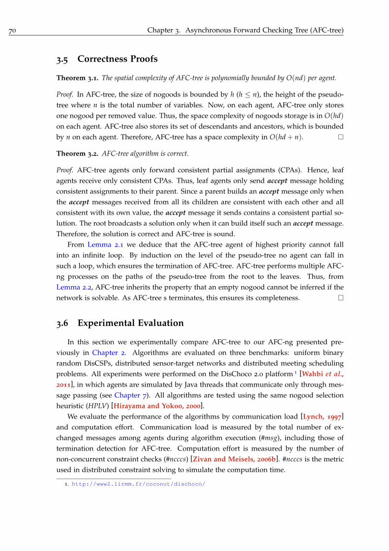
70 Chapter 3. Asynchronous Forward Checking Tree (AFC-tree)
3.5 Correctness Proofs
Theorem 3.1. The spatial complexity of AFC-tree is polynomially bounded by O(nd) per agent.
Proof. In AFC-tree, the size of nogoods is bounded by h (h ≤ n), the height of the pseudo-
tree where n is the total number of variables. Now, on each agent, AFC-tree only stores
one nogood per removed value. Thus, the space complexity of nogoods storage is in O(hd)
on each agent. AFC-tree also stores its set of descendants and ancestors, which is bounded
by n on each agent. Therefore, AFC-tree has a space complexity in O(hd + n).
Theorem 3.2. AFC-tree algorithm is correct.
Proof. AFC-tree agents only forward consistent partial assignments (CPAs). Hence, leaf
agents receive only consistent CPAs. Thus, leaf agents only send accept message holding
consistent assignments to their parent. Since a parent builds an accept message only when
the accept messages received from all its children are consistent with each other and all
consistent with its own value, the accept message it sends contains a consistent partial so-
lution. The root broadcasts a solution only when it can build itself such an accept message.
Therefore, the solution is correct and AFC-tree is sound.
From Lemma 2.1 we deduce that the AFC-tree agent of highest priority cannot fall
into an infinite loop. By induction on the level of the pseudo-tree no agent can fall in
such a loop, which ensures the termination of AFC-tree. AFC-tree performs multiple AFC-
ng processes on the paths of the pseudo-tree from the root to the leaves. Thus, from
Lemma 2.2, AFC-tree inherits the property that an empty nogood cannot be inferred if the
network is solvable. As AFC-tree s terminates, this ensures its completeness.
3.6 Experimental Evaluation
In this section we experimentally compare AFC-tree to our AFC-ng presented pre-
viously in Chapter 2. Algorithms are evaluated on three benchmarks: uniform binary
random DisCSPs, distributed sensor-target networks and distributed meeting scheduling
problems. All experiments were performed on the DisChoco 2.0 platform 1 [Wahbi et al.,
2011], in which agents are simulated by Java threads that communicate only through mes-
sage passing (see Chapter 7). All algorithms are tested using the same nogood selection
heuristic (HPLV) [Hirayama and Yokoo, 2000].
We evaluate the performance of the algorithms by communication load [Lynch, 1997]
and computation effort. Communication load is measured by the total number of ex-
changed messages among agents during algorithm execution (#msg), including those of
termination detection for AFC-tree. Computation effort is measured by the number of
non-concurrent constraint checks (#ncccs) [Zivan and Meisels, 2006b]. #ncccs is the metric
used in distributed constraint solving to simulate the computation time.
1. http://www2.lirmm.fr/coconut/dischoco/

3.6. Experimental Evaluation 71
3.6.1 Uniform binary random DisCSPs
The algorithms are tested on uniform binary random DisCSPs which are characterized
by �n, d, p1, p2�, where n is the number of agents/variables, d is the number of values in
each of the domains, p1 the network connectivity defined as the ratio of existing binary
constraints, and p2 the constraint tightness defined as the ratio of forbidden value pairs.
We solved instances of two classes of constraint graphs: sparse graphs �20, 10, 0.2, p2� and
dense ones �20, 10, 0.7, p2�. We vary the tightness from 0.1 to 0.9 by steps of 0.05. For each
pair of fixed density and tightness (p1, p2) we generated 25 instances, solved 4 times each.
We report average over the 100 runs.
0.0⋅100
1.0⋅103
2.0⋅103
3.0⋅103
4.0⋅103
5.0⋅103
6.0⋅103
7.0⋅103
8.0⋅103
9.0⋅103
0.1 0.2 0.3 0.4 0.5 0.6 0.7 0.8 0.9
#ncccs
p2
AFC-ng
AFC-tree
Figure 3.5 – The number of non-concurrent constraint checks (#ncccs) performed on sparseproblems (p1 = 0.2).
0.0⋅100
1.0⋅103
2.0⋅103
3.0⋅103
4.0⋅103
5.0⋅103
6.0⋅103
7.0⋅103
0.1 0.2 0.3 0.4 0.5 0.6 0.7 0.8 0.9
#m
sg
p2
AFC-ng
AFC-tree
Figure 3.6 – The total number of messages sent on sparse problems (p1 = 0.2).
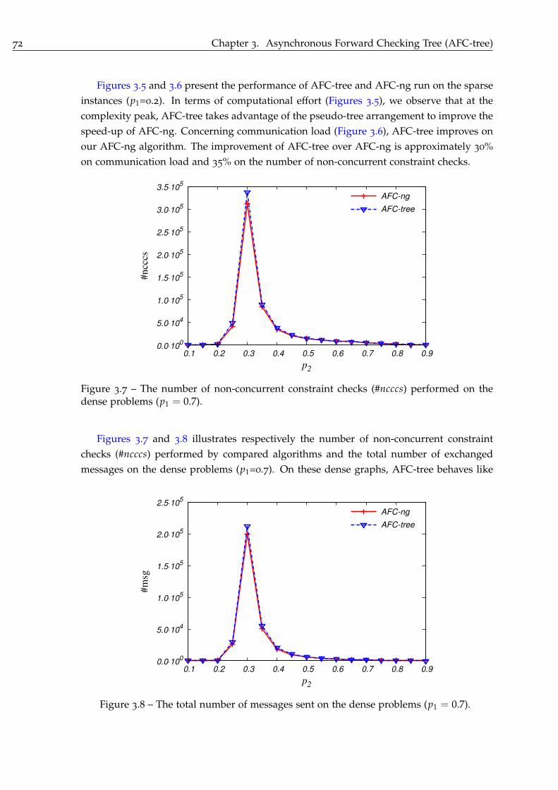
72 Chapter 3. Asynchronous Forward Checking Tree (AFC-tree)
Figures 3.5 and 3.6 present the performance of AFC-tree and AFC-ng run on the sparse
instances (p1=0.2). In terms of computational effort (Figures 3.5), we observe that at the
complexity peak, AFC-tree takes advantage of the pseudo-tree arrangement to improve the
speed-up of AFC-ng. Concerning communication load (Figure 3.6), AFC-tree improves on
our AFC-ng algorithm. The improvement of AFC-tree over AFC-ng is approximately 30%
on communication load and 35% on the number of non-concurrent constraint checks.
0.0⋅100
5.0⋅104
1.0⋅105
1.5⋅105
2.0⋅105
2.5⋅105
3.0⋅105
3.5⋅105
0.1 0.2 0.3 0.4 0.5 0.6 0.7 0.8 0.9
#ncccs
p2
AFC-ng
AFC-tree
Figure 3.7 – The number of non-concurrent constraint checks (#ncccs) performed on thedense problems (p1 = 0.7).
Figures 3.7 and 3.8 illustrates respectively the number of non-concurrent constraint
checks (#ncccs) performed by compared algorithms and the total number of exchanged
messages on the dense problems (p1=0.7). On these dense graphs, AFC-tree behaves like
0.0⋅100
5.0⋅104
1.0⋅105
1.5⋅105
2.0⋅105
2.5⋅105
0.1 0.2 0.3 0.4 0.5 0.6 0.7 0.8 0.9
#m
sg
p2
AFC-ng
AFC-tree
Figure 3.8 – The total number of messages sent on the dense problems (p1 = 0.7).

3.6. Experimental Evaluation 73
AFC-ng with a very slight domination of AFC-ng. This is AFC-tree does not benefit from
the pseudo-tree arrangement, which is like a chain-tree in such graphs.
3.6.2 Distributed Sensor Target Problems
The Distributed Sensor-Target Problem (SensorDisCSP) [Béjar et al., 2005] is a benchmark
based on a real distributed problem (see Section 1.3.2.2). It consists of n sensors that track m
targets. Each target must be tracked by 3 sensors. Each sensor can track at most one target.
A solution must satisfy visibility and compatibility constraints. The visibility constraint
defines the set of sensors to which a target is visible. The compatibility constraint defines
the compatibility among sensors. In our implementation of the DisCSP algorithms, the
encoding of the SensorDisCSP presented in Section 1.3.2.2 is translated to an equivalent
formulation where we have three virtual agents for every real agent, each virtual agent
handling a single variable.
Problems are characterized by �n, m, pc, pv�, where n is the number of sensors, m is the
number of targets, each sensor can communicate with a fraction pc of the sensors that are
in its sensing range, and each target can be tracked by a fraction pv of the sensors having
the target in their sensing range. We present results for the class � 25, 5, 0.4, pv�, where
we vary pv from 0.1 to 0.9 by steps of 0.05. Again, for each pair (pc, pv) we generated 25
instances, solved 4 times each, and averaged over the 100 runs.
0.0⋅100
2.0⋅105
4.0⋅105
6.0⋅105
8.0⋅105
1.0⋅106
1.2⋅106
0.1 0.2 0.3 0.4 0.5 0.6 0.7 0.8 0.9
#ncccs
pv
AFC-ng
AFC-tree
Figure 3.9 – Total number non-concurrent constraint checks performed on instances wherepc = 0.4.
We present the results obtained on the SensorDisCSP benchmark in Figures 3.9 and
Figure 3.10. Our experiments shows that AFC-tree outperforms AFC-ng algorithm when
comparing the computational effort (Figure 3.9). Concerning the communication load (Fig-
ure 3.10), the ranking of algorithms is similar to that on computational effort for the in-
stances at the complexity peak. However it is slightly dominated by the AFC-ng on the

74 Chapter 3. Asynchronous Forward Checking Tree (AFC-tree)
0.0⋅100
1.0⋅104
2.0⋅104
3.0⋅104
4.0⋅104
5.0⋅104
6.0⋅104
7.0⋅104
0.1 0.2 0.3 0.4 0.5 0.6 0.7 0.8 0.9
#m
sg
pv
AFC-ng
AFC-tree
Figure 3.10 – Total number of exchanged messages on instances where pc = 0.4.
exceptionally hard problems (pv = 1.5). Hence, AFC-tree remains the best on all problems
except for a single point (pv = 1.5), where AFC-ng shows a trivial improvement.
3.6.3 Distributed Meeting Scheduling Problems
The Distributed Meeting Scheduling Problem (DisMSP) is a truly distributed benchmark
where agents may not desire to deliver their personal information to a centralized agent
to solve the whole problem [Wallace and Freuder, 2002; Meisels and Lavee, 2004] (see
Section 1.3.2.1). The DisMSP consists of a set of n agents having a personal private calendar
and a set of m meetings each taking place in a specified location.
We encode the DisMSP in DisCSP as follows. Each DisCSP agent represents a real agent
and contains k variables representing the k meetings to which the agent participates. These
k meetings are selected randomly among the m meetings. The domain of each variable
contains the d × h slots where a meeting can be scheduled. A slot is one hour long, and
there are h slots per day and d days. There is an equality constraint for each pair of
variables corresponding to the same meeting in different agents. There is an arrival-time
constraint between all variables/meetings belonging to the same agent. We place meetings
randomly on the nodes of a uniform grid of size g × g and the traveling time between
two adjacent nodes is 1 hour. Thus, the traveling time between two meetings equals the
Euclidean distance between nodes representing the locations where they will be held. For
varying the tightness of the arrival-time constraint we vary the size of the grid on which
meetings are placed.
Problems are characterized by �n, m, k, d, h, g�, where n is the number of agents, m is
the number meetings, k is the number of meetings/variables per agent, d is the number of
days and h is the number of hours per day, and g is the grid size. The duration of each
meeting is one hour. In our implementation of the DisCSP algorithms, this encoding is
translated to an equivalent formulation where we have k (number of meetings per agent)
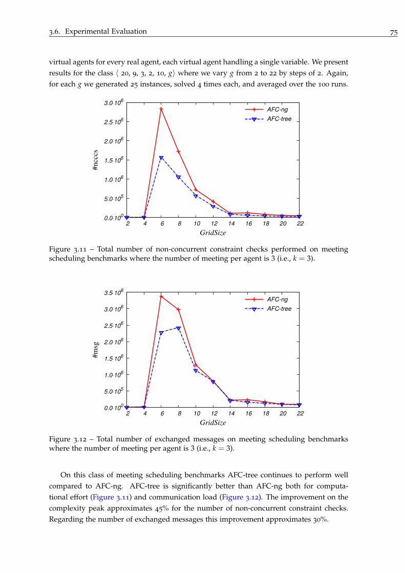
3.6. Experimental Evaluation 75
virtual agents for every real agent, each virtual agent handling a single variable. We present
results for the class � 20, 9, 3, 2, 10, g� where we vary g from 2 to 22 by steps of 2. Again,
for each g we generated 25 instances, solved 4 times each, and averaged over the 100 runs.
0.0⋅100
5.0⋅105
1.0⋅106
1.5⋅106
2.0⋅106
2.5⋅106
3.0⋅106
2 4 6 8 10 12 14 16 18 20 22
#ncccs
GridSize
AFC-ng
AFC-tree
Figure 3.11 – Total number of non-concurrent constraint checks performed on meetingscheduling benchmarks where the number of meeting per agent is 3 (i.e., k = 3).
0.0⋅100
5.0⋅105
1.0⋅106
1.5⋅106
2.0⋅106
2.5⋅106
3.0⋅106
3.5⋅106
2 4 6 8 10 12 14 16 18 20 22
#m
sg
GridSize
AFC-ng
AFC-tree
Figure 3.12 – Total number of exchanged messages on meeting scheduling benchmarkswhere the number of meeting per agent is 3 (i.e., k = 3).
On this class of meeting scheduling benchmarks AFC-tree continues to perform well
compared to AFC-ng. AFC-tree is significantly better than AFC-ng both for computa-
tional effort (Figure 3.11) and communication load (Figure 3.12). The improvement on the
complexity peak approximates 45% for the number of non-concurrent constraint checks.
Regarding the number of exchanged messages this improvement approximates 30%.

76 Chapter 3. Asynchronous Forward Checking Tree (AFC-tree)
3.6.4 Discussion
Our experiments demonstrates that AFC-tree is almost always better than or equivalent
to AFC-ng both in terms of communication load and computational effort. When the graph
is sparse, AFC-tree benefits from running separate search processes in disjoint problem
subtrees. When agents are highly connected (dense graphs), AFC-tree runs on a chain-tree
pseudo-tree and thus mimics AFC-ng.
3.7 Other Related Works
The Synchronous Backtracking (SBT) [Yokoo, 2000b] is the naive search method for
solving distributed CSPs. SBT is a decentralized extension of the chronological backtrack-
ing algorithm for centralized CSPs. Although this algorithm communicates only consistent
current partial assignments (CPA), it does not take advantage of parallelism, because the
problem is solved sequentially and only the agent holding the current partial assignments
is activated while other agents are in an idle state. Collin et al. (1991) proposed Network
Consistency Protocol (NCP) a variation of the synchronous backtracking. NCP agents are
prioritized using a depth-first search tree. Despite the fact that agents on the same branch
act synchronously, agents having the same parent can act concurrently. Thus, instead of
given the privilege to only one agent, as is done in SBT, an agent passes on the privilege of
extending the CPA or backtracking to all its children concurrently.
In Interleaved Asynchronous Backtracking (IDIBT) [Hamadi, 2002], agents partici-
pate in multiple processes of asynchronous backtracking. Each agent keeps a separate
AgentView for each search process in IDIBT. The number of search processes is fixed by
the first agent in the ordering. The performance of concurrent asynchronous backtrack-
ing [Hamadi, 2002] was tested and found to be ineffective for more than two concurrent
search processes [Hamadi, 2002].
3.8 Summary
A new complete, asynchronous algorithm, which needs polynomial space is presented.
This algorithm called Asynchronous Forward-Checking Tree (AFC-tree), is based on our
nogood-based Asynchronous Forward Checking (AFC-ng) and is performed on a pseudo-
tree arrangement of the constraint graph. AFC-tree runs simultaneous AFC-ng processes
on each branch of the pseudo-tree to exploit the parallelism inherent in the problem. Our
experiments show that AFC-tree is more robust than AFC-ng. It is particularly good when
the problems are sparse because it takes advantage of the pseudo-tree ordering.

4Maintaining Arc Consistency
Asynchronously in Synchronous
Distributed Search
Contents6.1 Introduction . . . . . . . . . . . . . . . . . . . . . . . . . . . . . . . . . . . . . . . . . . 107
6.2 Background . . . . . . . . . . . . . . . . . . . . . . . . . . . . . . . . . . . . . . . . . . . 108
6.3 ABT_DO-Retro May Not Terminate . . . . . . . . . . . . . . . . . . . . . . . . . . . . 110
6.4 The Right Way to Compare Orders . . . . . . . . . . . . . . . . . . . . . . . . . . . . 112
6.5 Summary . . . . . . . . . . . . . . . . . . . . . . . . . . . . . . . . . . . . . . . . . . . . . 114
We presented in (Chapter 2) our Nogood-Based Asynchronous Forward Checking
(AFC-ng). AFC-ng is an efficient and robust algorithm for solving Distributed Con-
straint Satisfaction Problems (DisCSPs). AFC-ng performs an asynchronous forward check-
ing phase during synchronous search. In this chapter, we propose two new algorithms
based on the same mechanism as AFC-ng. However, instead of using forward checking
as a filtering property, we propose to maintain arc consistency asynchronously (MACA).
The first algorithm we propose, MACA-del, enforces arc consistency thanks to an addi-
tional type of messages, deletion messages. The second algorithm, MACA-not, achieves
arc consistency without any new type of message. We provide a theoretical analysis and
an experimental evaluation of the proposed approach. Our experiments show the good
performance of MACA algorithms, particularly those of MACA-not.
This chapter is organized as follows. Section 4.1 introduces the previous works for
maintenance of arc consistency in DisCSPs and situates our contribution in the domain.
Section 4.2 recalls the necessary background on MAC. Sections 4.3 describes the MACA-
del and MACA-not algorithms. Theoretical analysis and correctness proofs are given in
Section 4.4. Section 4.5 presents an experimental evaluation of our proposed algorithms
against state-of-the-art other algorithms. Finally, we will conclude this chapter in Sec-
tion 4.6.
77

78 Chapter 4. Maintaining Arc Consistency Asynchronously in Synchronous Distributed Search
4.1 Introduction
We presented in Chapter 1 many backtrack search algorithms that were developed
for solving constraint satisfaction problems. Typical backtrack search algorithms try to
build a solution to a CSP by interleaving variable instantiation with constraint propaga-
tion. Forward Checking (FC) [Haralick and Elliott, 1980] and Maintaining Arc Consis-
tency (MAC) [Sabin and Freuder, 1994] are examples of such algorithms. In the 80’s, FC
was considered as the most efficient search algorithm. In the middle 90’s, several works
have empirically shown that MAC is more efficient than FC on hard and large problems[Bessiere and Régin, 1996; Grant and Smith, 1996].
Although, many studies incorporated FC successfully in distributed CSPs [Brito and
Meseguer, 2003; Meisels and Zivan, 2007; Ezzahir et al., 2009], MAC has not yet been well
investigated. The only tentatives to include arc consistency maintenance in distributed al-
gorithms were done on the Asynchronous Backtracking algorithm. Silaghi et al. (2001b)
introduced the Distributed Maintaining Asynchronously Consistency for ABT, (DMAC-
ABT), the first algorithm able to maintain arc consistency in distributed CSPs [Silaghi et
al., 2001b]. DMAC-ABT considers consistency maintenance as a hierarchical nogood-based
inference. Brito and Meseguer (2008) proposed ABT-uac and ABT-dac, two algorithms that
connect ABT with arc consistency [Brito and Meseguer, 2008]. ABT-uac propagates uncon-
ditionally deleted values to enforce an amount of full arc consistency. ABT-dac propagates
conditionally and unconditionally deleted values using directional arc consistency. ABT-
uac shows minor improvement in communication load and ABT-dac is harmful in many
instances.
In this chapter, we propose two new synchronous search algorithms based on the same
mechanism as AFC-ng. However, instead of maintaining forward checking asynchronously
on agents not yet instantiated, we propose to maintain arc consistency asynchronously
on these future agents. We call this new scheme MACA, for maintaining arc consistency
asynchronously. As in AFC-ng, only the agent holding the current partial assignment (CPA)
can perform an assignment. However, unlike AFC-ng, MACA attempts to maintain the
arc consistency instead of performing only FC. The first algorithm we propose, MACA-
del, enforces arc consistency thanks to an additional type of messages, deletion messages
(del). Hence, whenever values are removed during a constraint propagation step, MACA-
del agents notify other agents that may be affected by these removals, sending them a
del message. del messages contain all removed values and the nogood justifying their
removal. The second algorithm, MACA-not, achieves arc consistency without any new type
of message. We achieve this by storing all deletions performed by an agent on domains
of its neighboring agents, and sending this information to these neighbors within the CPA
message.

4.2. Maintaining Arc Consistency 79
4.2 Maintaining Arc Consistency
Constraint propagation is a central feature of efficiency for solving CSPs [Bessiere,
2006]. The oldest and most commonly used technique for propagating constraints is arc
consistency (AC).
The Maintaining Arc Consistency (MAC) algorithm [Sabin and Freuder, 1994] alter-
nates exploration steps and constraint propagation steps. That is, at each step of the search,
a variable assignment is followed by a filtering process that corresponds to enforcing arc
consistency. For implementing MAC in a distributed CSP, Each agent Ai is assumed to
know all constraints in which it is involved and the agents with whom it shares a con-
straint (i.e., Γ(xi)). These agents and the constraints linking them to Ai form the local
constraint network of Ai, denoted by CSP(i).
Definition 4.1 The local constraint network CSP(i) of an agent Ai ∈ A consists of all con-
straints involving xi and all variables of these constraints (i.e., its neighbors).
In order to allow agents to maintain arc consistency in distributed CSPs, our proposed
approach consists in enforcing arc consistency on the local constraint network of each agent.
Basically, each agent Ai stores locally copies of all variables in CSP(i). We also assume that
each agent knows the neighborhood it has in common with its own neighbors, without
knowing the constraints relating them. That is, for each of its neighbors Ak, an agent Ai
knows the list of agents Aj such that there is a constraint between xi and xj and a constraint
between xk and xj.
Agent Ai stores nogoods for its removed values. They are stored in NogoodStore[xi].
But in addition to nogoods stored for its own values, Ai needs to store nogoods for values
removed from variables xj in CSP(i). Nogoods justifying the removals of values from D(xj)
are stored in NogoodStore[xj]. Hence, the NogoodStore of an agent Ai is a vector of several
NogoodStores, one for each variable in CSP(i).
4.3 Maintaining Arc Consistency Asynchronously
In AFC-ng, the forward checking phase aims at anticipating the backtrack. Neverthe-
less, we do not take advantage of the value removals caused by FC if it does not completely
wipe out the domain of the variable. One can investigate these removals by enforcing arc
consistency. This is motivated by the fact that the propagation of a value removal, for
an agent Ai, may generate an empty domain for a variable in its local constraint network
CSP(i). We can then detect an earlier dead-end and then anticipate as soon as possible the
backtrack operation.
In synchronous search algorithms for solving DisCSPs, agents sequentially assign their
variables. Thus, agents perform the assignment of their variable only when they hold the
current partial assignment, CPA. We propose an algorithm in which agents assign their
variable one by one following a total ordering on agents. Hence, whenever an agent suc-
ceeds in extending the CPA by assigning its variable on it, it sends the CPA to its successor
to extend it. Copies of this CPA are also sent to the other agents whose assignments are not
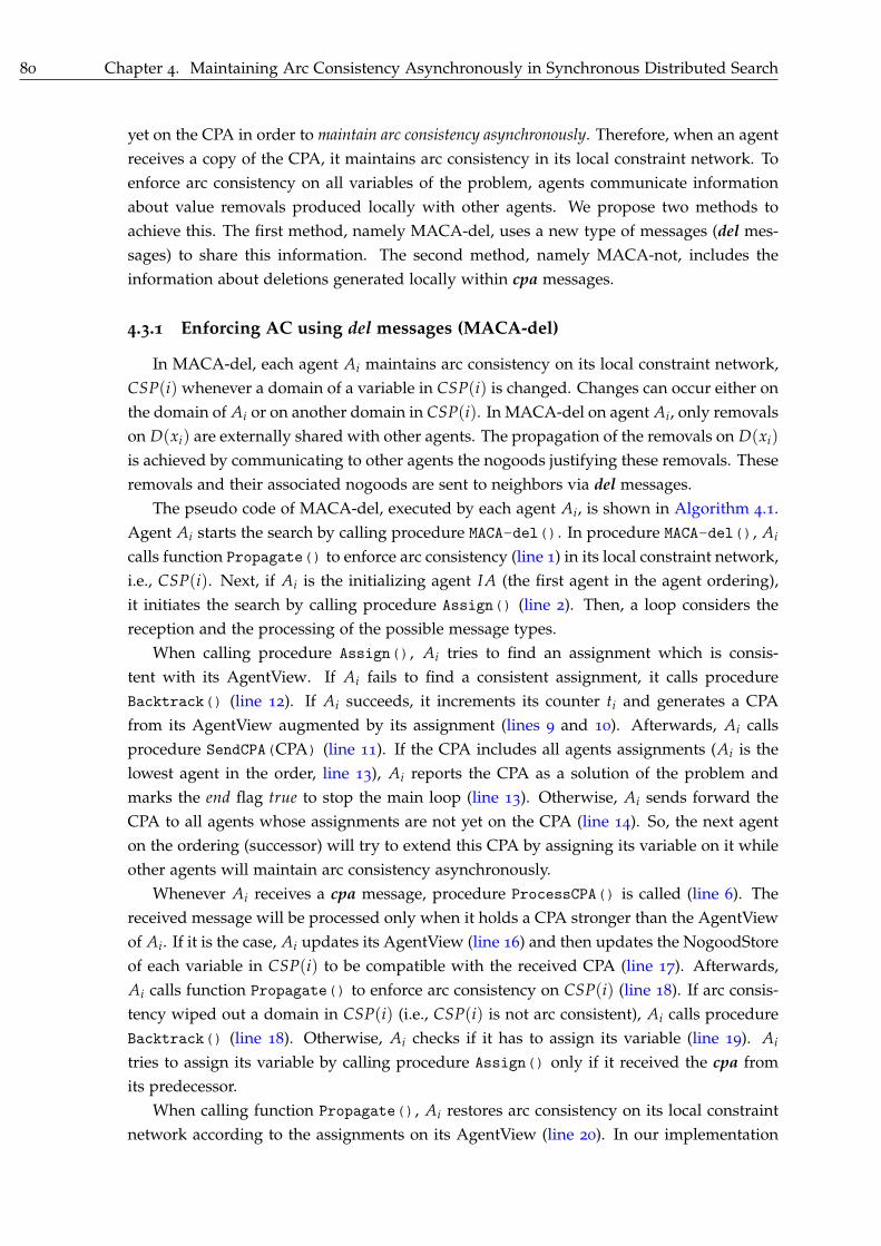
80 Chapter 4. Maintaining Arc Consistency Asynchronously in Synchronous Distributed Search
yet on the CPA in order to maintain arc consistency asynchronously. Therefore, when an agent
receives a copy of the CPA, it maintains arc consistency in its local constraint network. To
enforce arc consistency on all variables of the problem, agents communicate information
about value removals produced locally with other agents. We propose two methods to
achieve this. The first method, namely MACA-del, uses a new type of messages (del mes-
sages) to share this information. The second method, namely MACA-not, includes the
information about deletions generated locally within cpa messages.
4.3.1 Enforcing AC using del messages (MACA-del)
In MACA-del, each agent Ai maintains arc consistency on its local constraint network,
CSP(i) whenever a domain of a variable in CSP(i) is changed. Changes can occur either on
the domain of Ai or on another domain in CSP(i). In MACA-del on agent Ai, only removals
on D(xi) are externally shared with other agents. The propagation of the removals on D(xi)
is achieved by communicating to other agents the nogoods justifying these removals. These
removals and their associated nogoods are sent to neighbors via del messages.
The pseudo code of MACA-del, executed by each agent Ai, is shown in Algorithm 4.1.
Agent Ai starts the search by calling procedure MACA-del(). In procedure MACA-del(), Ai
calls function Propagate() to enforce arc consistency (line 1) in its local constraint network,
i.e., CSP(i). Next, if Ai is the initializing agent IA (the first agent in the agent ordering),
it initiates the search by calling procedure Assign() (line 2). Then, a loop considers the
reception and the processing of the possible message types.
When calling procedure Assign(), Ai tries to find an assignment which is consis-
tent with its AgentView. If Ai fails to find a consistent assignment, it calls procedure
Backtrack() (line 12). If Ai succeeds, it increments its counter ti and generates a CPA
from its AgentView augmented by its assignment (lines 9 and 10). Afterwards, Ai calls
procedure SendCPA(CPA) (line 11). If the CPA includes all agents assignments (Ai is the
lowest agent in the order, line 13), Ai reports the CPA as a solution of the problem and
marks the end flag true to stop the main loop (line 13). Otherwise, Ai sends forward the
CPA to all agents whose assignments are not yet on the CPA (line 14). So, the next agent
on the ordering (successor) will try to extend this CPA by assigning its variable on it while
other agents will maintain arc consistency asynchronously.
Whenever Ai receives a cpa message, procedure ProcessCPA() is called (line 6). The
received message will be processed only when it holds a CPA stronger than the AgentView
of Ai. If it is the case, Ai updates its AgentView (line 16) and then updates the NogoodStore
of each variable in CSP(i) to be compatible with the received CPA (line 17). Afterwards,
Ai calls function Propagate() to enforce arc consistency on CSP(i) (line 18). If arc consis-
tency wiped out a domain in CSP(i) (i.e., CSP(i) is not arc consistent), Ai calls procedure
Backtrack() (line 18). Otherwise, Ai checks if it has to assign its variable (line 19). Ai
tries to assign its variable by calling procedure Assign() only if it received the cpa from
its predecessor.
When calling function Propagate(), Ai restores arc consistency on its local constraint
network according to the assignments on its AgentView (line 20). In our implementation
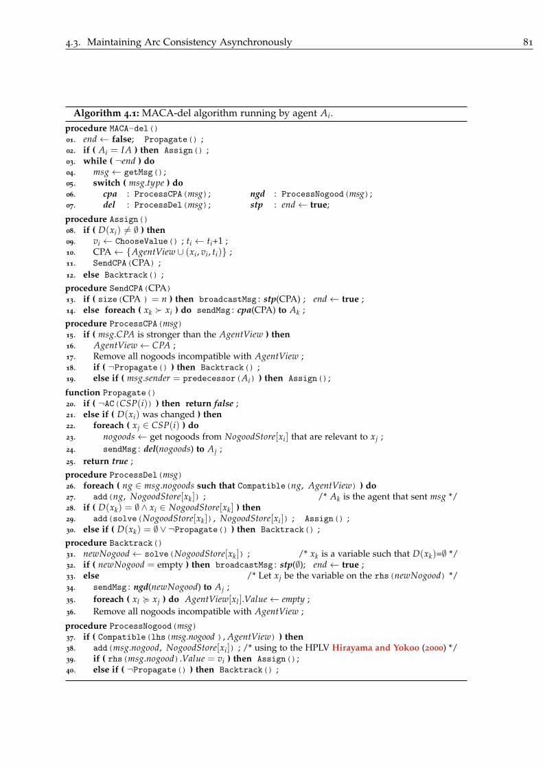
4.3. Maintaining Arc Consistency Asynchronously 81
Algorithm 4.1: MACA-del algorithm running by agent Ai.procedure MACA-del()
01. end ← false; Propagate() ;02. if ( Ai = IA ) then Assign() ;03. while ( ¬end ) do04. msg ← getMsg();05. switch ( msg.type ) do06. cpa : ProcessCPA(msg); ngd : ProcessNogood(msg);07. del : ProcessDel(msg); stp : end ← true;
procedure Assign()
08. if ( D(xi) �= ∅ ) then09. vi ← ChooseValue() ; ti ← ti+1 ;10. CPA ← {AgentView ∪ (xi , vi , ti)} ;11. SendCPA(CPA) ;12. else Backtrack() ;procedure SendCPA(CPA)13. if ( size(CPA ) = n ) then broadcastMsg : stp(CPA) ; end ← true ;14. else foreach ( xk � xi ) do sendMsg : cpa(CPA) to Ak ;procedure ProcessCPA(msg)15. if ( msg.CPA is stronger than the AgentView ) then16. AgentView ← CPA ;17. Remove all nogoods incompatible with AgentView ;18. if ( ¬Propagate() ) then Backtrack() ;19. else if ( msg.sender = predecessor(Ai) ) then Assign();
function Propagate()
20. if ( ¬AC(CSP(i)) ) then return false ;21. else if ( D(xi) was changed ) then22. foreach ( xj ∈ CSP(i) ) do
23. nogoods ← get nogoods from NogoodStore[xi] that are relevant to xj ;24. sendMsg : del(nogoods) to Aj ;25. return true ;procedure ProcessDel(msg)26. foreach ( ng ∈ msg.nogoods such that Compatible(ng, AgentView) ) do27. add(ng, NogoodStore[xk]) ; /* Ak is the agent that sent msg */28. if ( D(xk) = ∅∧ xi ∈ NogoodStore[xk] ) then29. add(solve(NogoodStore[xk]), NogoodStore[xi]) ; Assign() ;30. else if ( D(xk) = ∅∨ ¬Propagate() ) then Backtrack() ;procedure Backtrack()
31. newNogood ← solve(NogoodStore[xk]) ; /* xk is a variable such that D(xk)=∅ */32. if ( newNogood = empty ) then broadcastMsg : stp(∅); end ← true ;33. else /* Let xj be the variable on the rhs(newNogood) */34. sendMsg : ngd(newNogood) to Aj ;35. foreach ( xl � xj ) do AgentView[xl ].Value ← empty ;36. Remove all nogoods incompatible with AgentView ;
procedure ProcessNogood(msg)37. if ( Compatible(lhs(msg.nogood ), AgentView) ) then38. add(msg.nogood, NogoodStore[xi]) ; /* using to the HPLV Hirayama and Yokoo (2000) */39. if ( rhs(msg.nogood).Value = vi ) then Assign();40. else if ( ¬Propagate() ) then Backtrack() ;
82 Chapter 4. Maintaining Arc Consistency Asynchronously in Synchronous Distributed Search
we used AC-2001 [Bessiere and Régin, 2001] to enforce arc consistency but any generic AC
algorithm can be used. MACA-del requires from the algorithm enforcing arc consistency
to store a nogood for each removed value. When two nogoods are possible for the same
value, we select the best with the Highest Possible Lowest Variable heuristic [Hirayama and
Yokoo, 2000]. If enforcing arc consistency on CSP(i) has failed, i.e., a domain was wiped
out, the function returns f alse (line 20). Otherwise, if the domain of xi was changed (i.e.,
there are some deletions to propagate), Ai informs its constrained agents by sending them
del messages that contain nogoods justifying these removals (lines 23-24). Finally, the
function returns true (line 25). When sending a del message to a neighboring agent Aj,
only nogoods such that all variables in their left hand sides have a higher priority than Aj
will be communicated to Aj. Furthermore, all nogoods having the same left hand side are
factorized in one single nogood whose right hand side is the set of all values removed by
this left hand side.
Whenever Ai receives a del message, it adds to the NogoodStore of the sender, say Ak,
(i.e., NogoodStore[xk]) all nogoods compatible with the AgentView of Ai (lines 26-27). Af-
terward, Ai checks if the domain of xk is wiped out (i.e., the remaining values in D(xk) are
removed by nogoods that have just been received from Ak) and xi belongs to the Nogood-
Store of xk (i.e., xi is already assigned and its current assignment is included in at least one
nogood removing a value from D(xk)) (line 28). If it is the case, Ai removes its current value
by storing the resolved nogood from the NogoodStore of xk (i.e., solve(NogoodStore[xk]))
as justification of this removal, and then calls procedure Assign() to try an other value
(line 29). Otherwise, when D(xk) is wiped-out (xi is not assigned) or if a dead-end occurs
when trying to enforce arc consistency, Ai has to backtrack and thus it calls procedure
Backtrack() (line 30).
Each time a dead-end occurs on a domain of a variable xk in CSP(i) (including xi), the
procedure Backtrack() is called. The nogoods that generated the dead-end are resolved
by computing a new nogood newNogood (line 31). newNogood is the conjunction of the
left hand sides of all these nogoods stored by Ai in NogoodStore[xk]. If the new nogood
newNogood is empty, Ai terminates execution after sending a stp message to all agents in
the system meaning that the problem is unsolvable (line 32). Otherwise, Ai backtracks by
sending a ngd message to agent Aj, the owner of the variable on the right hand side of
newNogood (line 34). Next, Ai updates its AgentView in order to keep only assignments
of agents that are placed before Aj in the total ordering (line 35). Ai also updates the
NogoodStore of all variables in CSP(i) by removing nogoods incompatible with its new
AgentView (line 36).
Whenever a ngd message is received, Ai checks the validity of the received nogood
(line 37). If the received nogood is compatible with its AgentView, Ai adds this nogood to
its NogoodStore (i.e. NogoodStore[xi], line 38). Then, Ai checks if the value on the right
hand side of the received nogood equals its current value (vi). If it is the case, Ai calls
the procedure Assign() to try another value for its variable (line 39). Otherwise, Ai calls
function Propagate() to restore arc consistency. When a dead-end was generated in its
local constraint network, Ai calls procedure Backtrack() (line 40).

4.3. Maintaining Arc Consistency Asynchronously 83
4.3.2 Enforcing AC without additional kind of message (MACA-not)
In the following, we show how to enforce arc consistency without additional kind of
messages. In MACA-del, global consistency maintenance is achieved by communicating to
constrained agents (agents in CSP(i)) all values pruned from D0(xi). This may generate
many del messages in the network, and then result in a communication bottleneck. In
addition, many del messages may lead agents to perform more efforts to process them. In
MACA-not, communicating the removals produced in CSP(i) is delayed until the agent Ai
wants to send a cpa message. When sending the cpa message to a lower priority agent Ak,
agent Ai attaches nogoods justifying value removals from CSP(i) to the cpa message. But
it does not attach all of them because some variables are irrelevant to Ak (not connected to
xk by a constraint).
MACA-not shares with Ak all nogoods justifying deletions on variables not yet instan-
tiated that share a constraint with both Ai and Ak (i.e., variables in {CSP(i) ∩ CSP(k)} \
vars(CPA )). Thus, when Ak receives the cpa it receives also deletions performed in CSP(i)
that can lead him to more arc consistency propagation.
Algorithm 4.2: New lines/procedures for MACA-not with respect to MACA-del.procedure MACA-not()
01. end ← false; Propagate() ;02. if ( Ai = IA ) then Assign() ;03. while ( ¬end ) do04. msg ← getMsg();05. switch ( msg.type ) do06. cpa : ProcessCPA(msg); ngd : ProcessNogood(msg);07. stp : end ← true;
procedure SendCPA(CPA)08. if ( size(CPA ) = n ) then broadcastMsg : stp(CPA) ; end ← true ;09. else10. foreach ( xk � xi ) do11. nogoods ← ∅;12. foreach ( xj ∈ {CSP(i) ∩ CSP(k)} such that xj � xi ) do
13. nogoods ← nogoods ∪ getNogoods(xj) ;14. sendMsg : cpa(CPA, nogoods) to Ak ;
procedure ProcessCPA(msg)15. if ( msg.CPA is stronger than the AgentView ) then16. AgentView ← CPA ;17. Remove all nogoods incompatible with AgentView ;18. foreach ( nogoods ∈ msg.nogoods ) do add(nogoods, NogoodStore) ;19. if ( ¬Propagate() ) then Backtrack() ;20. else if ( msg.sender = predecessor(Ai) ) then Assign();
function Propagate()
21. return AC(CSP(i)) ;
We present in Algorithm 4.2 the pseudo-code of MACA-not algorithm. Only proce-
dures that are new or different from those of MACA-del in Algorithm 4.1 are presented.
Function Propagate() no longer sends del messages, it just maintains arc consistency on
CSP(i) and returns true iff no domain was wiped out.
In procedure SendCPA(CPA), when sending a cpa message to an agent Ak, Ai attaches

84 Chapter 4. Maintaining Arc Consistency Asynchronously in Synchronous Distributed Search
to the CPA the nogoods justifying the removals from the domains of variables in CSP(i)
constrained with Ak (lines 10-14, Algorithm 4.2).
Whenever Ai receives a cpa message, procedure ProcessCPA() is called (line 6). The
received message will be processed only when it holds a CPA stronger than the AgentView
of Ai. If it is the case, Ai updates its AgentView (line 16) and then updates the NogoodStore
to be compatible with the received CPA (line 17). Next, all nogoods contained in the
received message are added to the NogoodStore (line 18). Obviously, nogoods are added
to the NogoodStore referring to the variable in their right hand side (i.e., ng is added to
NogoodStore[xj] if xj is the variable in rhs(ng)). Afterwards, Ai calls function Propagate()
to restore arc consistency in CSP(i) (line 19). If a domain of a variable in CSP(i) wiped
out, Ai calls procedure Backtrack() (line 19). Otherwise, Ai checks if it has to assign its
variable (line 20). Ai tries to assign its variable by calling procedure Assign() only if it
received the cpa from its predecessor.
4.4 Theoretical analysis
We demonstrate that MACA is sound, complete and terminates, with a polynomial
space complexity.
Lemma 4.1. MACA is guaranteed to terminate.
Proof. (Sketch) The proof is close to the one given in Lemma 2.1, Chapter 2. It can easily
be obtained by induction on the agent ordering that there will be a finite number of new
generated CPAs (at most nd, where n the number of variables and d is the maximum
domain size), and that agents can never fall into an infinite loop for a given CPA.
Lemma 4.2. MACA cannot infer inconsistency if a solution exists.
Proof. Whenever a stronger cpa or a ngd message is received, MACA agents update their
NogoodStores. In MACA-del, the nogoods contained in del are accepted only if they are
compatible with AgentView (line 27, Algorithm 4.1). In MACA-not, the nogoods included
in the cpa messages are compatible with the received CPA and they are accepted only when
the CPA is stronger than AgentView (line 15, Algorithm 4.2). Hence, for every CPA that
may potentially lead to a solution, agents only store valid nogoods. Since all additional
nogoods are generated by logical inference when a domain wipe-out occurs, the empty
nogood cannot be inferred if the network is satisfiable.
Theorem 4.1. MACA is correct.
Proof. The argument for soundness is close to the one given in Theorem 2.2, Chapter 2.
The fact that agents only forward consistent partial solution on the cpa messages at only
one place in procedure Assign() (line 11, Algorithm 4.1), implies that the agents receive
only consistent assignments. A solution is found by the last agent only in procedure
SendCPA(CPA) at (line 13, Algorithm 4.1 and line 8, Algorithm 4.2). At this point, all
agents have assigned their variables, and their assignments are consistent. Thus MACA is

4.5. Experimental Results 85
sound. Completeness comes from the fact that MACA is able to terminate and does not
report inconsistency if a solution exists (Lemma 4.1 and 4.2).
Theorem 4.2. MACA is polynomial in space.
Proof. On each agent, MACA stores one nogood of size at most n per removed value in its
local constraint network. The local constraint network contains at most n variables. Thus,
the space complexity of MACA is in O(n2d) on each agent where d is the maximal initial
domain size.
Theorem 4.3. MACA messages are polynomially bounded.
Proof. The largest messages for MACA-del are del messages. In the worst-case, a del mes-
sage contains a nogood for each value. Thus, the size of del messages is in O(nd). In
MACA-not, the largest messages are cpa messages. The worst-case is a cpa message con-
taining a CPA and one nogood for each value of each variable in the local constraint net-
work. Thus, the size of a cpa message is in O(n + n2d) = O(n2d).
4.5 Experimental Results
In this section we experimentally compare MACA algorithms to ABT-uac, ABT-
dac [Brito and Meseguer, 2008] and AFC-ng Chapter 2. These algorithms are evaluated
on uniform random binary DisCSPs. All experiments were performed on the DisChoco 2.0
platform 1 [Wahbi et al., 2011], in which agents are simulated by Java threads that commu-
nicate only through message passing. All algorithms are tested on the same static agents
ordering (lexicographic ordering) and the same nogood selection heuristic (HPLV) [Hi-
rayama and Yokoo, 2000]. For ABT-dac we implemented an improved version of Silaghi’s
solution detection [Silaghi, 2006] and counters for tagging assignments.
We evaluate the performance of the algorithms by communication load [Lynch, 1997]
and computation effort. Communication load is measured by the total number of ex-
changed messages among agents during algorithm execution (#msg), including those of
termination detection (system messages). Computation effort is measured by the number
of non-concurrent constraint checks (#ncccs) [Zivan and Meisels, 2006b]. #ncccs is the
metric used in distributed constraint solving to simulate the computation time.
The algorithms are tested on uniform random binary DisCSPs which are characterized
by �n, d, p1, p2�, where n is the number of agents/variables, d is the number of values in
each of the domains, p1 the network connectivity defined as the ratio of existing binary
constraints, and p2 the constraint tightness defined as the ratio of forbidden value pairs.
We solved instances of two classes of constraint networks: sparse networks �20, 10, 0.25, p2�
and dense ones �20, 10, 0.7, p2�. We vary the tightness from 0.1 to 0.9 by steps of 0.1. For
each pair of fixed density and tightness (p1, p2) we generated 100 instances. The average
over the 100 instances is reported.
1. http://www.lirmm.fr/coconut/dischoco/

86 Chapter 4. Maintaining Arc Consistency Asynchronously in Synchronous Distributed Search
0.0⋅100
2.0⋅104
4.0⋅104
6.0⋅104
8.0⋅104
1.0⋅105
1.2⋅105
1.4⋅105
1.6⋅105
1.8⋅105
0.1 0.2 0.3 0.4 0.5 0.6 0.7 0.8 0.9
#ncccs
p2
AFC-ng
ABT-uac
ABT-dac
MACA-del
MACA-not
Figure 4.1 – The number of non-concurrent constraint checks (#ncccs) performed for solvingsparse problems (p1 = 0.25).
First, we present the performance of the algorithms on the sparse instances, p1 = 0.25,
(Figures 4.1 and 4.2). Concerning the computational effort (Figure 4.1), algorithms enforc-
ing an amount of arc consistency are better than AFC-ng, which only enforces forward
checking. Among these algorithms MACA-del is the fastest one. MACA-not behaves like
ABT-dac, which is better than ABT-uac.
0.0⋅100
1.0⋅105
2.0⋅105
3.0⋅105
4.0⋅105
5.0⋅105
6.0⋅105
7.0⋅105
8.0⋅105
9.0⋅105
0.1 0.2 0.3 0.4 0.5 0.6 0.7 0.8 0.9
#m
sg
p2
AFC-ng
ABT-uac
ABT-dac
MACA-del
MACA-not
Figure 4.2 – The total number of messages sent for solving sparse problems (p1 = 0.25).
Concerning the communication load (Figure 4.2), algorithms performing an amount of
arc consistency improve on AFC-ng by an even larger scale than for computational effort.
ABT-uac and ABT-dac require almost the same number of exchanged messages. Among the
algorithms maintaining an amount of arc consistency, the algorithms with a synchronous
behavior (MACA algorithms) outperform those with an asynchronous behavior (ABT-dac

4.5. Experimental Results 87
and ABT-uac) by a factor of 6. It thus seems that on sparse problems, maintaining arc
consistency in synchronous search algorithms provides more benefit than in asynchronous
ones. MACA-not exchanges slightly fewer messages than MACA-del at the complexity
peak.
0.0⋅100
2.0⋅105
4.0⋅105
6.0⋅105
8.0⋅105
1.0⋅106
1.2⋅106
1.4⋅106
1.6⋅106
0.1 0.2 0.3 0.4 0.5 0.6 0.7 0.8 0.9
#ncccs
p2
AFC-ng
ABT-uac
ABT-dac
MACA-del
MACA-not
Figure 4.3 – The number of non-concurrent constraint checks (#ncccs) performed for solvingdense problems (p1 = 0.7).
In the following, we present the performance of the algorithms on the dense instances
(p1 = 0.7). Concerning the computational effort (Figure 4.3), the first observation is that
asynchronous algorithms are less efficient than those performing assignments sequentially.
Among all compared algorithms, AFC-ng is the fastest one on these dense problems. This
is consistent with results on centralized CSPs where FC had a better behavior on dense
problems than on sparse ones [Bessiere and Régin, 1996; Grant and Smith, 1996]. As on
sparse problems, ABT-dac outperforms ABT-uac. Conversely to sparse problems, MACA-
not outperforms MACA-del.
Concerning the communication load (Figure 4.4), on dense problems, asynchronous al-
gorithms (ABT-uac and ABT-dac) require a large number of exchanged messages. MACA-
del does not improve on AFC-ng because of a too large number of exchanged del messages.
On these problems, MACA-not is the algorithm that requires the smallest number of mes-
sages. MACA-not improves on synchronous algorithms (AFC-ng and MACA-del) by a
factor of 11 and on asynchronous algorithms (ABT-uac and ABT-dac) by a factor of 40.
4.5.1 Discussion
From these experiments we can conclude that in synchronous algorithms, maintaining
arc consistency is better than maintaining forward checking in terms of computational
effort when the network is sparse, and is always better in terms of communication load.
We can also conclude that maintaining arc consistency in synchronous algorithms produces

88 Chapter 4. Maintaining Arc Consistency Asynchronously in Synchronous Distributed Search
0.0⋅100
5.0⋅105
1.0⋅106
1.5⋅106
2.0⋅106
2.5⋅106
3.0⋅106
3.5⋅106
0.1 0.2 0.3 0.4 0.5 0.6 0.7 0.8 0.9
#m
sg
p2
AFC-ng
ABT-uac
ABT-dac
MACA-del
MACA-not
Figure 4.4 – The total number of messages sent for solving dense problems (p1 = 0.7).
much larger benefits than maintaining arc consistency in asynchronous algorithms like
ABT.
4.6 Summary
We have proposed two new synchronous search algorithms for solving DisCSPs. These
are the first attempts to maintain arc consistency during synchronous search in DisCSPs.
The first algorithm, MACA-del, enforces arc consistency thanks to an additional type of
messages, deletion messages. The second algorithm, MACA-not, achieves arc consistency
without any new type of message. Despite the synchronicity of search, these two algo-
rithms perform the arc consistency phase asynchronously. Our experiments show that
maintaining arc consistency during synchronous search produces much larger benefits
than maintaining arc consistency in asynchronous algorithms like ABT. The communi-
cation load of MACA-del can be significantly lower than that of AFC-ng, the best syn-
chronous algorithm to date. MACA-not shows even larger improvements thanks to its
more parsimonious use of messages.

5Agile Asynchronous BackTracking
(Agile-ABT)
Contents7.1 Introduction . . . . . . . . . . . . . . . . . . . . . . . . . . . . . . . . . . . . . . . . . . 115
7.2 Architecture . . . . . . . . . . . . . . . . . . . . . . . . . . . . . . . . . . . . . . . . . . 116
7.2.1 Communication System . . . . . . . . . . . . . . . . . . . . . . . . . . . . . . . . 117
7.2.2 Event Management . . . . . . . . . . . . . . . . . . . . . . . . . . . . . . . . . . . 118
7.2.3 Observers in layers . . . . . . . . . . . . . . . . . . . . . . . . . . . . . . . . . . . 118
7.3 Using DisChoco 2.0 . . . . . . . . . . . . . . . . . . . . . . . . . . . . . . . . . . . . . . 119
7.4 Experimentations . . . . . . . . . . . . . . . . . . . . . . . . . . . . . . . . . . . . . . . 121
7.5 Conclusion . . . . . . . . . . . . . . . . . . . . . . . . . . . . . . . . . . . . . . . . . . . 123
It is known from centralized CSPs that reordering variables dynamically improves the
efficiency of the search procedure. Moreover, reordering in ABT is required in various
applications (e.g., security [Silaghi et al., 2001a]). All polynomial space algorithms pro-
posed so far to improve Asynchronous Backtracking by reordering agents during search
only allow a limited amount of reordering Section 1.4.3. In this chapter, we propose Agile-
ABT, a search procedure that is able to change the ordering of agents more than previous
approaches. This is done via the original notion of termination value, a vector of stamps
labeling the new orders exchanged by agents during search. In Agile-ABT, agents can re-
order themselves as much as they want as long as the termination value decreases as the
search progresses. Agents cooperate without any global control to reduce termination val-
ues rapidly, gaining efficiency while ensuring polynomial space complexity. We compare
the performance of Agile-ABT with other algorithms and our experiments show the good
performance of Agile-ABT when compared to other dynamic reordering techniques.
The rest of the chapter is organized as follows. Section 5.1 introduces and situates our
contribution (Agile-ABT). Section 5.2 describes the concepts needed to select new orders
that decrease the termination value. We give the details of our algorithm in Section 5.3 and
we prove it in Section 5.4. An experimental evaluation is given in Section 5.5. Section 5.7
concludes the chapter.
89
90 Chapter 5. Agile Asynchronous BackTracking (Agile-ABT)
5.1 Introduction
Several distributed algorithms for solving DisCSPs have been developed, among which
Asynchronous Backtracking (ABT) is the central one [Yokoo et al., 1998; Bessiere et al.,
2005]. ABT is an asynchronous algorithm executed autonomously by each agent in the
distributed problem. In ABT, the priority order of agents is static, and an agent tries to
find an assignment satisfying the constraints with higher priority agents. When an agent
sets a variable value, the selected value will not be changed unless an exhaustive search is
performed by lower priority agents. Now, it is known from centralized CSPs that adapting
the order of variables dynamically during search drastically fastens the search procedure.
Moreover, reordering in ABT is required in various applications (e.g., security [Silaghi et
al., 2001a]).
Asynchronous Weak Commitment (AWC) dynamically reorders agents during search
by moving the sender of a nogood higher in the order than the other agents in the nogood[Yokoo, 1995]. But AWC requires exponential space for storing nogoods. Silaghi et al.
(2001c) tried to hybridize ABT with AWC. Abstract agents fulfill the reordering operation
to guarantee a finite number of asynchronous reordering operations. In [Silaghi, 2006], the
heuristic of the centralized dynamic backtracking [Ginsberg, 1993] was applied to ABT.
However, in both studies, the improvement obtained on ABT was minor.
Zivan and Meisels (2006a) proposed another algorithm for Dynamic Ordering in Asyn-
chronous Backtracking (ABT_DO). When an agent assigns a value to its variable, ABT_DO
can reorder only lower priority agents. A new kind of ordering heuristics for ABT_DO is
presented in [Zivan et al., 2009]. These heuristics, called retroactive heuristics ABT_DO-
Retro, enable the generator of the nogood to be moved to a higher position than that of
the target of the backtrack. The degree of flexibility of these heuristics is dependent on
the size of the nogood storage capacity, which is predefined. Agents are limited to store
nogoods equal or smaller than a predefined size K. The space complexity of the agents is
thus exponential in K. However, the best heuristic, ABT_DO-Retro-MinDom, proposed in[Zivan et al., 2009] is a heuristic that does not require this exponential storage of nogoods.
In ABT_DO-Retro-MinDom, the agent that generates a nogood is placed in the new order
between the last and the second last agents in the nogood if its domain size is smaller than
that of the agents it passes on the way up.
In this chapter, we propose Agile Asynchronous Backtracking (Agile-ABT), an asyn-
chronous dynamic ordering algorithm that does not follow the standard restrictions in
asynchronous backtracking algorithms. The order of agents appearing before the agent
receiving a backtrack message can be changed with a great freedom while ensuring poly-
nomial space complexity. Furthermore, that agent receiving the backtrack message, called
the backtracking target, is not necessarily the agent with the lowest priority within the
conflicting agents in the current order. The principle of Agile-ABT is built on termina-
tion values exchanged by agents during search. A termination value is a tuple of positive
integers attached to an order. Each positive integer in the tuple represents the expected cur-
rent domain size of the agent in that position in the order. Orders are changed by agents
without any global control so that the termination value decreases lexicographically as the

5.2. Introductory Material 91
search progresses. Since, a domain size can never be negative, termination values cannot
decrease indefinitely. An agent informs the others of a new order by sending them its new
order and its new termination value. When an agent compares two contradictory orders,
it keeps the order associated with the smallest termination value.
5.2 Introductory Material
In Agile-ABT, all agents start with the same order O. Then, agents are allowed to
change the order asynchronously. Each agent Ai ∈ A stores a unique order denoted by Oi.
Oi is called the current order of Ai. Agents appearing before Ai in Oi are the higher priority
agents (predecessors) denoted by O−i and conversely the lower priority agents (successors)
O+i are agents appearing after Ai.
Agents can infer inconsistent sets of assignments, called nogoods. A nogood can be
represented as an implication. There are clearly many different ways of representing a
given nogood as an implication. For example, ¬[(xi=vi) ∧ (xj=vj) ∧ · · · ∧ (xk=vk)] is logi-
cally equivalent to [(xj=vj) ∧ · · · ∧ (xk=vk)] → (xi �= vi). When a nogood is represented
as an implication, the left hand side (lhs) and the right hand side (rhs) are defined from the
position of →. A nogood ng is relevant with respect to an order Oi if all agents in lhs(ng)
appear before rhs(ng) in Oi.
The current domain of xi is the set of values vi ∈ D0(xi) such that xi �= vi does not
appear in any of the right hand sides of the nogoods stored by Ai. Each agent keeps only
one nogood per removed value. The size of the current domain of Ai is denoted by di (i.e.,
|D(xi)| = di). The initial domain size of a variable xi, before any value has been pruned, is
denoted by d0i (i.e., d0
i = |D0(xi)| and di = |D(xi)|).
Before presenting Agile-ABT, we need to introduce new notions and to present some
key subfunctions.
5.2.1 Reordering details
In order to allow agents to asynchronously propose new orders, they must be able to
coherently decide which order to select. We propose that the priority between the different
orders is based on termination values. Informally, if Oi = [A1, . . . , An] is the current order
known by an agent Ai, then the tuple of domain sizes [d1, . . . , dn] is the termination value
of Oi on Ai. To build termination values, agents need to know the current domain sizes of
other agents. To this end, agents exchange explanations.
Definition 5.1 An explanation ej is an expression lhs(ej) → dj, where lhs(ej) is the conjunc-
tion of the left hand sides of all nogoods stored by Aj as justifications of value removals for xj, and
dj is the number of values not pruned by nogoods in the domain of Aj. dj is the right hand side of
ej, rhs(ej).
Each time an agent communicates its assignment to other agents (by sending them an
ok? message, see Section 5.3), it inserts its explanation in the ok? message for allowing
other agents to build their termination value.
92 Chapter 5. Agile Asynchronous BackTracking (Agile-ABT)
The variables in the left hand side of an explanation ej must precede the variable xj
in the order because the assignments of these variables have been used to determine the
current domain of xj. An explanation ej induces ordering constraints, called safety conditions
in [Ginsberg and McAllester, 1994] (see Section 1.2.1.4).
Definition 5.2 A safety condition is an assertion xk ≺ xj. Given an explanation ej, S(ej) is the
set of safety conditions induced by ej, where S(ej)={(xk ≺ xj) | xk ∈ lhs(ej)}.
An explanation ej is relevant to an order O if all variables in lhs(ej) appear before xj
in O. Each agent Ai stores a set Ei of explanations sent by other agents. During search, Ei
is updated to remove explanations that are no longer valid.
Definition 5.3 An explanation ej in Ei is valid on agent Ai if it is relevant to the current order
Oi and lhs(ej) is compatible with the AgentView of Ai.
When Ei contains an explanation ej associated with Aj, Ai uses this explanation to
justify the size of the current domain of Aj. Otherwise, Ai assumes that the size of the
current domain of Aj is equal to its initial domain size d0j . The termination value depends
on the order and the set of explanations.
Definition 5.4 Let Ei be the set of explanations stored by Ai, O be an order on the agents such that
every explanation in Ei is relevant to O, and O(k) be such that AO(k) is the kth agent in O. The
termination value TV(Ei,O) is the tuple [tv1, . . . , tvn], where tvk = rhs(eO(k)) if eO(k) ∈ Ei,
otherwise, tvk = d0O(k).
In Agile-ABT, an order Oi is always associated with a termination value TVi. When
comparing two orders the strongest order is that associated with the lexicographically
smallest termination value. In case of ties, we use the lexicographic order on agents IDs, the
smaller being the stronger.
Example 5.1 Consider for instance the two orders O1=[A1, A2, A5, A4, A3] and
O2=[A1, A2, A4, A5, A3]. If the termination value associated with O1 is equal to the termi-
nation value associated with O2, O2 is stronger than O1 because the vector [1, 2, 4, 5, 3] of
IDs in O2 is lexicographically smaller than the vector [1, 2, 5, 4, 3] of IDs in O1.
In the following we will show that the interest of the termination values is not limited
to the role of establishing a priority between the different orders proposed by agents. We
use them to provide more flexibility in the choice of the backtracking target and to speed
up the search.
5.2.2 The Backtracking Target
When all the values of an agent Ai are ruled out by nogoods, these nogoods are re-
solved, producing a new nogood newNogood. newNogood is the conjunction of the left
hand side (lhs) of all nogoods stored by Ai. If newNogood is empty, then the inconsistency
is proved. Otherwise, one of the conflicting agents must change its value. In standard
ABT, the backtracking target (i.e., the agent that must change its value) is the agent with

5.2. Introductory Material 93
the lowest priority. Agile-ABT overcomes this restriction by allowing Ai to select with great
freedom the backtracking target. When a new nogood newNogood is produced by resolu-
tion, the only condition to choose a variable xk as the backtracking target (i.e., the variable
to put in the right hand side of newNogood) is to find an order O� such that TV(up_Ei,O�)
is lexicographically smaller than the termination value associated with the current order of
Ai (i.e., Oi). up_Ei is obtained by updating Ei after placing xk in rhs(newNogood).
Function UpdateExplanations takes as arguments the set of explanations stored by
Ai (i.e., Ei), the generated nogood newNogood and the variable xk to place in the right
hand side (rhs) of newNogood. UpdateExplanations removes all explanations that are
no longer compatible with the AgentView of Ai after placing xk in the right hand side of
newNogood. (The assignment of xk will be removed from AgentView after backtracking).
Next, it updates the explanation of agent Ak stored in Ai and it returns a set of (updated)
explanations up_Ei.
Algorithm 5.1: Function Update Explanations.function UpdateExplanations(Ei , newNogood, xk)
01. up_Ei ← Ei ;02. SetRhs(newNogood, xk) ;03. remove each ej ∈ up_Ei such that xk ∈ lhs(ej) ;04. if ( ek /∈up_Ei ) then
05. ek ← {∅ → d0k} ;
06. add(ek, up_Ei) ;07. e�k ← {[lhs(ek)∪ lhs(newNogood )] → rhs(ek)− 1} ;08. replace ek by e�k ;09. return up_Ei;
This function does not create cycles in the set of safety conditions S(up_Ei) if S(Ei)
is acyclic. Indeed, all the explanations added or removed from S(Ei) to obtain S(up_Ei)
contain xk. Hence, if S(up_Ei) contains cycles, all these cycles should contain xk. However,
there does not exist any safety condition of the form xk ≺ xj in S(up_Ei) because all of
these explanations have been removed in line 3. Thus, S(up_Ei) cannot be cyclic. As we
will show in Section 5.3, the updates performed by Ai ensure that S(Ei) always remains
acyclic. As a result, S(up_Ei) is acyclic as well, and it can be represented by a directed
acyclic graph−→G = (X−→
G, E−→
G) where X−→
G= X = {x1, . . . , xn}. An edge (xj, xl) ∈ E−→
Gif the
safety condition (xj ≺ xl) ∈ S(up_Ei), i.e., el ∈ up_Ei and xj ∈ lhs(el). Any topological
sort of−→G is an order relevant to the safety conditions induced by up_Ei.
To recap, when all values of an agent Ai are ruled out by some nogoods, they are
resolved, producing a new nogood (newNogood). In Agile-ABT, Ai can select with great
freedom the variable xk whose value is to be changed. The only restriction to place a
variable xk in the rhs(newNogood) is to find an order O� such that TV(up_Ei,O�) is lex-
icographically smaller than the termination value associated with the current order of Ai.
Note that up_Ei being acyclic, there are always one or more topological orders that agree
with S(up_Ei). In the following, we will discuss in more details how to choose the order
O�.

94 Chapter 5. Agile Asynchronous BackTracking (Agile-ABT)
5.2.3 Decreasing termination values
Termination of Agile-ABT is based on the fact that the termination values associated
with orders selected by agents decrease as search progresses. To speed up the search,
Agile-ABT is written so that agents decrease termination values whenever they can. When
an agent resolves its nogoods, it checks whether it can find a new order of agents such
that the associated termination value is smaller than that of the current order. If so, the
agent will replace its current order and termination value by those just computed, and will
inform all other agents.
Algorithm 5.2: Function Compute Order.function ComputeOrder(up_Ei)
10.−→G = (X−→
G, E−→
G) is the acyclic directed graph associated to up_Ei ;
11. p ← 1 ;12. O is an array of length n ;
13. while (−→G �= ∅ ) do
14. Roots ← {xj ∈ X−→G
| xj has no incoming edges} ;15. O(p) ← xj such that dj = min{dk | xk ∈ Roots} ;
16. remove xj from−→G ; /* with all outgoing edges from xj */
17. p ← p + 1 ;18. return O ;
Assume that after resolving its nogoods, an agent Ai, decides to place xk in the
right hand side of the nogood (newNogood) produced by the resolution and let Ei =
UpdateExplanations(Ei, newNogood, xk). The function ComputeOrder takes as parame-
ter the set up_Ei and returns an order O relevant to the partial ordering induced by up_Ei.
Let−→G be the acyclic directed graph associated with up_Ei. The function ComputeOrder
works by determining, at each iteration p, the set Roots of vertexes that have no prede-
cessor (line 14). As we aim at minimizing the termination value, function ComputeOrder
selects the vertex xj in Roots that has the smallest domain size (line 15). This vertex is
placed at the pth position. Finally, p is incremented after removing xj and all outgoing
edges from xj from−→G (lines 16-17).
Algorithm 5.3: Function Choose Variable Ordering.function ChooseVariableOrder(Ei , newNogood)19. O� ← Oi; TV� ← TVi; E � ← nil; x� ← nil ;20. foreach ( xk ∈ newNogood ) do21. up_Ei ← UpdateExplanations(Ei , newNogood, xk) ;22. up_O ← ComputeOrder(up_Ei) ;23. up_TV ← TV(up_Ei, up_O ) ;24. if ( up_TV is smaller than TV� ) then25. x� ← xk;26. O� ← up_O;27. TV� ← up_TV;28. E � ← up_Ei ;29. return �x�,O�, TV�, E ��;
Having proposed an algorithm that determines an order with small termination value
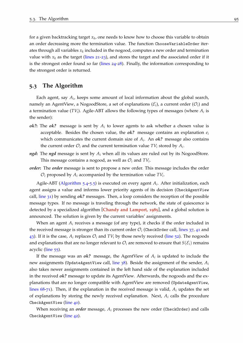
5.3. The Algorithm 95
for a given backtracking target xk, one needs to know how to choose this variable to obtain
an order decreasing more the termination value. The function ChooseVariableOrder iter-
ates through all variables xk included in the nogood, computes a new order and termination
value with xk as the target (lines 21-23), and stores the target and the associated order if it
is the strongest order found so far (lines 24-28). Finally, the information corresponding to
the strongest order is returned.
5.3 The Algorithm
Each agent, say Ai, keeps some amount of local information about the global search,
namely an AgentView, a NogoodStore, a set of explanations (Ei), a current order (Oi) and
a termination value (TVi). Agile-ABT allows the following types of messages (where Ai is
the sender):
ok?: The ok? message is sent by Ai to lower agents to ask whether a chosen value is
acceptable. Besides the chosen value, the ok? message contains an explanation ei
which communicates the current domain size of Ai. An ok? message also contains
the current order Oi and the current termination value TVi stored by Ai.
ngd: The ngd message is sent by Ai when all its values are ruled out by its NogoodStore.
This message contains a nogood, as well as Oi and TVi.
order: The order message is sent to propose a new order. This message includes the order
Oi proposed by Ai accompanied by the termination value TVi.
Agile-ABT (Algorithm 5.4-5.5) is executed on every agent Ai. After initialization, each
agent assigns a value and informs lower priority agents of its decision (CheckAgentView
call, line 31) by sending ok? messages. Then, a loop considers the reception of the possible
message types. If no message is traveling through the network, the state of quiescence is
detected by a specialized algorithm [Chandy and Lamport, 1985], and a global solution is
announced. The solution is given by the current variables’ assignments.
When an agent Ai receives a message (of any type), it checks if the order included in
the received message is stronger than its current order Oi (CheckOrder call, lines 37, 41 and
43). If it is the case, Ai replaces Oi and TVi by those newly received (line 52). The nogoods
and explanations that are no longer relevant to Oi are removed to ensure that S(Ei) remains
acyclic (line 55).
If the message was an ok? message, the AgentView of Ai is updated to include the
new assignments (UpdateAgentView call, line 38). Beside the assignment of the sender, Ai
also takes newer assignments contained in the left hand side of the explanation included
in the received ok? message to update its AgentView. Afterwards, the nogoods and the ex-
planations that are no longer compatible with AgentView are removed (UpdateAgentView,
lines 68-71). Then, if the explanation in the received message is valid, Ai updates the set
of explanations by storing the newly received explanation. Next, Ai calls the procedure
CheckAgentView (line 40).
When receiving an order message, Ai processes the new order (CheckOrder) and calls
CheckAgentView (line 42).

96 Chapter 5. Agile Asynchronous BackTracking (Agile-ABT)
Algorithm 5.4: The Agile-ABT algorithm executed by an agent Ai (Part 1).procedure Agile-ABT()
30. ti ← 0; TVi ← [∞, ∞, . . . , ∞]; end ← false; vi ← empty ;31. CheckAgentView() ;32. while ( ¬end ) do33. msg ← getMsg();34. switch ( msg.type ) do35. ok? : ProcessInfo(msg); ngd : ResolveConflict(msg);36. order : ProcessOrder(msg); stp : end ← true;
procedure ProcessInfo(msg)37. CheckOrder(msg.Order, msg.TV) ;38. UpdateAgentView(msg.Assig ∪ lhs(msg.Exp)) ;39. if ( msg.Exp is valid ) then add(msg.Exp, Ei);40. CheckAgentView() ;procedure ProcessOrder(msg)41. CheckOrder(msg.Order,msg.TV) ;42. CheckAgentView() ;procedure ResolveConflict(msg)43. CheckOrder(msg.Order,msg.TV) ;44. UpdateAgentView(msg.Assig ∪ lhs(msg.Nogood)) ;45. if ( Compatible(msg.Nogood, AgentView ∪ myAssig) ) then46. if ( Relevant(msg.Nogood,Oi) ) then47. add(msg.Nogood,NogoodStore) ;48. vi ← empty ;49. CheckAgentView() ;50. else if ( rhs(msg.Nogood) = vi ) then51. sendMsg : ok?(myAssig, ei ,Oi , TVi) to msg.Sender
procedure CheckOrder(O�, TV�)
52. if ( O�is stronger than Oi ) then53. Oi ← O� ;54. TVi ← TV� ;55. remove nogoods and explanations non relevant to Oi ;
procedure CheckAgentView()
56. if ( (¬isConsistent(vi , AgentView) ) then57. vi ← ChooseValue() ;58. if ( vi ) then59. foreach ( xk � xi ) do60. sendMsg : ok?(myAssig, ei ,Oi , TVi) to Ak ;61. else Backtrack() ;62. else if ( Oi was modified ) then63. foreach ( xk � xi ) do64. sendMsg : ok?(myAssig, ei ,Oi , TVi) to Ak ;
procedure UpdateAgentView(Assignments)65. foreach ( xj ∈ Assignments ) do
66. if ( Assignments[j].tag > AgentView[j].tag ) then67. AgentView[j] ← Assignments[j] ;68. foreach ( ng ∈ NogoodStore such that ¬Compatible(lhs(ng), AgentView) ) do69. remove(ng,myNogoodStore) ;70. foreach ( ej ∈ Ei such that ¬Compatible(lhs(ej), AgentView) ) do
71. remove(ej, Ei) ;

5.3. The Algorithm 97
When Ai receives a ngd message, it calls CheckOrder and UpdateAgentView (lines 43
and 44). The nogood contained in the message is accepted if it is compatible with the
AgentView and the assignment of xi and relevant to the current order of Ai. Otherwise,
the nogood is discarded and an ok? message is sent to the sender as in ABT (lines 50
and 51). When the nogood is accepted, it is stored, acting as justification for removing
the current value of Ai (line 47). A new value consistent with the AgentView is searched
(CheckAgentView call, line 49).
The procedure CheckAgentView checks if the current value vi is consistent with the
AgentView. If vi is consistent, Ai checks if Oi was modified (line 62). If so, Ai must
send its assignment to lower priority agents through ok? messages. If vi is not consistent
with its AgentView, Ai tries to find a consistent value (ChooseValue call, line 57). In this
process, some values of Ai may appear as inconsistent. In this case, the nogoods justifying
their removal are added to the NogoodStore (line 92 of function ChooseValue()). If a new
consistent value is found, an explanation ei is built and the new assignment is notified to
the lower priority agents of Ai through ok? messages (line 60). Otherwise, every value of
Ai is forbidden by the NogoodStore and Ai has to backtrack (Backtrack call, line 61).
In procedure Backtrack(), Ai resolves its nogoods, deriving a new nogood
(newNogood). If newNogood is empty, the problem has no solution. Ai terminates ex-
ecution after sending a stp message (lines 74-75). Otherwise, one of the agents included in
newNogood must change its value. The function ChooseVariableOrder selects the variable
to be changed (xk) and a new order (O�) such that the new termination value TV � is as
Algorithm 5.5: The Agile-ABT algorithm executed by an agent Ai (Part 2).procedure Backtrack()
72. newNogood ← solve(NogoodStore) ;73. if ( newNogood = empty ) then74. end ← true;75. sendMsg : stp( ) to system agent ;76. �xk ,O�, TV�, E �� ← ChooseVariableOrder(Ei , newNogood) ;77. if ( TV� is smaller than TVi ) then78. TVi ← TV� ;79. Oi ← O� ;80. Ei ← E � ;81. SetRhs(newNogood, xk) ;82. sendMsg : ngd(newNogood,Oi , TVi) to Ak ;83. remove ek from Ei ;84. broadcastMsg : order(Oi , TVi) ;85. else86. SetRhs(newNogood, xk) ; /* xk is the lower agent in newNogood */87. sendMsg : ngd(newNogood,Oi , TVi) to Ak ;88. UpdateAgentView (xk ← unknown) ;89. CheckAgentView() ;function ChooseValue()
90. foreach ( v ∈ D(xi) ) do91. if ( isConsistent(v, AgentView ) ) then return v;92. else store the best nogood for v ;93. return empty;

98 Chapter 5. Agile Asynchronous BackTracking (Agile-ABT)
small as possible. If TV � is smaller than that stored by Ai, the current order and the
current termination value are replaced by O� and TV � and Ai updates its explanations by
that returned by ChooseVariableOrder (lines 78-80). Then, a ngd message is sent to the
agent Ak owner of xk (line 82). ek is removed from Ei since Ak will probably change its
explanation after receiving the nogood (line 83). Afterwards, Ai sends an order message to
all other agents (line 84). When TV � is not smaller than the current termination value, Ai
cannot propose a new order and the variable to be changed (xk) is the variable that has the
lowest priority according to the current order of Ai (lines 86 and 87). Next, the assignment
of xk (the target of the backtrack) is removed from the AgentView of Ai (line 88). Finally,
the search is continued by calling the procedure CheckAgentView (line 89).
5.4 Correctness and complexity
In this section we demonstrate that Agile-ABT is sound, complete and terminates, and
that its space complexity is polynomially bounded.
Theorem 5.1. The spatial complexity of Agile-ABT is polynomial.
Proof. The size of nogoods, explanations, termination values, and orderings, is bounded by
n, the total number of variables. Now, on each agent, Agile-ABT only stores one nogood
per value, one explanation per agent, one termination value and one ordering. Thus, the
space complexity of Agile-ABT is in O(nd + n2 + n + n) = O(nd + n2) on each agent.
Theorem 5.2. The algorithm Agile-ABT is sound.
Proof. Let us assume that the state of quiescence is reached. The order (say O ) known by
all agents is the same because when an agent proposes a new order, it sends it to all other
agents. Obviously, O is the strongest order that has ever been calculated by agents. Also,
the state of quiescence implies that every pair of constrained agents satisfies the constraint
between them. To prove this, assume that there exist some constraints that are not satisfied.
This implies that there are at least two agents Ai and Ak that do not satisfy the constraint
between them (i.e., cik). Let Ai be the agent which has the highest priority between the two
agents according to O. Let vi be the current value of Ai when the state of quiescence is
reached (i.e., vi is the most up to date assignment of Ai) and let M be the last ok? message
sent by Ai before the state of quiescence is reached. Clearly, M contains vi, otherwise, Ai
would have sent another ok? message when it chose vi. Moreover, when M was sent,
Ai already knew the order O, otherwise Ai would have sent another ok? message when
it received (or generated) O. Ai sent M to all its successors according to O (including
Ak). The only case where Ak can forget vi after receiving it is the case where Ak derives a
nogood proving that vi is not feasible. In this case, Ak should send a nogood message to Ai.
If the nogood message is accepted by Ai, Ai must send an ok? message to its successors
(and therefore M is not the last one). Similarly, if the nogood message is discarded, Ai
have to re-send an ok? message to Ak (and therefore M is not the last one). So the state of
quiescence implies that Ak knows both O and vi. Thus, the state of quiescence implies that

5.4. Correctness and complexity 99
the current value of Ak is consistent with vi, otherwise Ak would send at least a message
and our quiescence assumption would be broken.
Theorem 5.3. The algorithm Agile-ABT is complete.
Proof. All nogoods are generated by logical inferences from existing constraints. Therefore,
an empty nogood cannot be inferred if a solution exists.
The proof of termination is built on Lemma 5.1 and 5.2.
Lemma 5.1. For any agent Ai, while a solution is not found and the inconsistency of the
problem is not proved, the termination value stored by Ai decreases after a finite amount
of time.
Proof. Let TVi = [tv1, . . . , tvn] be the current termination value of Ai. Assume that Ai
reaches a state where it cannot improve its termination value. If another agent succeeds in
generating a termination value smaller than TVi, Lemma 5.1 holds since Ai will receive the
new termination value. Now assume that Agile-ABT reaches a state σ where no agent can
generate a termination value smaller than TVi. We show that Agile-ABT will exit σ after a
finite amount of time. Let t be the time when Agile-ABT reaches the state σ. After a finite
time δt, the termination value of each agent Aj∈{1,...,n} will be equal to TVi, either because
Aj has generated itself a termination value equal to TVi or because Aj has received TVi in
an order message. Let O be the lexicographically smallest order among the current orders
of all agents at time t + δt. The termination value associated with O is equal to TVi. While
Agile-ABT is getting stuck in σ, no agent will be able to propose an order stronger than O
because no agent is allowed to generate a new order with the same termination value as
the one stored (line 77, Algorithm 5.5). Thus, after a finite time δ�t, all agents will receive
O. They will take it as their current order and Agile-ABT will behave as ABT, which is
known to be complete and to terminate.
We know that d0O(1) − tv1 values have been removed once and for all from the domain
of the variable xO(1) (i.e., d0O(1) − tv1 nogoods with empty lhs have been sent to AO(1)).
Otherwise, the generator of O could not have put AO(1) in the first position. Thus, the
domain size of xO(1) cannot be greater than tv1 (dO(1) ≤ tv1). After a finite amount
of time, if a solution is not found and the inconsistency of the problem is not proved,
a nogood–with an empty left hand side – will be sent to AO(1) which will cause it to
replace its assignment and to reduce its current domain size (d�O(1) = dO(1) − 1). The new
assignment and the new current domain size of AO(1) will be sent to the (n − 1) lower
priority agents. After receiving this message, we are sure that any generator of a new
nogood (say Ak) will improve the termination value. Indeed, when Ak resolves its nogoods,
it computes a new order such that its termination value is minimal. At worst, Ak can
propose a new order where AO(1) keeps its position. Even in this case the new termination
value TV �k = [d�O(1), . . . ] is lexicographically smaller than TVi = [tv1, . . . ] because d�O(1) =
dO(1)− 1 ≤ tv1 − 1. After a finite amount of time, all agents (Ai included) will receive TV �k .
This will cause Ai to update its termination value and to exit the state σ. This completes
the proof.

100 Chapter 5. Agile Asynchronous BackTracking (Agile-ABT)
Lemma 5.2. Let TV = [tv1, . . . , tvn] be the termination value associated with the current
order of any agent. We have tvj ≥ 0, ∀j ∈ 1..n
Proof. Let Ai be the agent that generated TV. We first prove that Ai never stores an expla-
nation with a rhs smaller than 1. An explanation ek stored by Ai was either sent by Ak or
generated when calling ChooseVariableOrder. If ek was sent by Ak, we have rhs(ek) ≥ 1
because the size of the current domain of any agent is always greater than or equal to
1. If ek was computed by ChooseVariableOrder, the only case where rhs(ek) is made
smaller than the right hand side of the previous explanation stored for Ak by Ai is in
(line 7 of UpdateExplanations. This happens when xk is selected to be the backtrack-
ing target (lines 21 and 28 of ChooseVariableOrder) and in such a case, the explanation
ek is removed just after sending the nogood message to Ak (line 83, Algorithm 5.5, of
Backtrack()). Hence, Ai never stores an explanation with a rhs equal to zero.
We now prove that it is impossible that Ai generated TV with tvj< 0 for some j. From
the point of view of Ai, tvj is the size of the current domain of AO(j). If Ai does not
store any explanation for AO(j) at the time it computes TV, Ai assumes that tvj is equal to
d0O(j) ≥ 1. Otherwise, tvj is equal to rhs(eO(j)), where eO(j) was either already stored by
Ai or generated when calling ChooseVariableOrder. Now, we know that every explanation
ek stored by Ai has rhs(ek) ≥ 1 and we know that ChooseVariableOrder cannot generate
an explanation e�k with rhs(e�k) < rhs(ek)− 1, where ek was the explanation stored by
Ai (line 7 of UpdateExplanations). Therefore, we are guaranteed that TV is such that
tvj ≥ 0, ∀j ∈ 1..n.
Theorem 5.4. The algorithm Agile-ABT terminates.
Proof. The termination value of any agent decreases lexicographically and does not stay
infinitely unchanged (Lemma 5.1). A termination value [tv1, . . . , tvn] cannot decrease in-
finitely because ∀i ∈ {1, . . . , n}, we have tvi ≥ 0 (Lemma 5.2). Hence the theorem.
5.5 Experimental Results
We compared Agile-ABT to ABT, ABT_DO, and ABT_DO-Retro (ABT_DO with retroac-
tive heuristics). All experiments were performed on the DisChoco 2.0 [Wahbi et al., 2011]
platform 1, in which agents are simulated by Java threads that communicate only through
message passing. We evaluate the performance of the algorithms by communication load
and computation effort. Communication load is measured by the total number of messages
exchanged among agents during algorithm execution (#msg), including termination detec-
tion (system messages). Computation effort is measured by an adaptation of the number
of non-concurrent constraint checks (generic number of non-concurrent constraint checks
#gncccs [Zivan and Meisels, 2006b]).
For ABT, we implemented the standard version where we use counters for tagging
assignments. For ABT_DO [Zivan and Meisels, 2006a], we implemented the best version,
using the nogood-triggered heuristic where the receiver of a nogood moves the sender to be
1. http://www.lirmm.fr/coconut/dischoco/

5.5. Experimental Results 101
in front of all other lower priority agents (denoted by ABT_DO-ng). For ABT_DO with
retroactive heuristics [Zivan et al., 2009], we implemented the best version, in which a
nogood generator moves itself to be in a higher position between the last and the second
last agents in the generated nogood 2. However, it moves before an agent only if its current
domain is smaller than the domain of that agent (denoted by ABT_DO-Retro-MinDom).
5.5.1 Uniform binary random DisCSPs
The algorithms are tested on uniform binary random DisCSPs characterized by
�n, d, p1, p2�, where n is the number of agents/variables, d the number of values per
variable, p1 the network connectivity defined as the ratio of existing binary constraints,
and p2 the constraint tightness defined as the ratio of forbidden value pairs. We solved
instances of two classes of problems: sparse problems �20, 10, 0.2, p2� and dense problems
�20, 10, 0.7, p2�. We vary the tightness p2 from 0.1 to 0.9 by steps of 0.1. For each pair
of fixed density and tightness (p1, p2) we generated 25 instances, solved 4 times each. We
report average over the 100 runs.
0.0⋅100
5.0⋅104
1.0⋅105
1.5⋅105
2.0⋅105
2.5⋅105
3.0⋅105
0.1 0.2 0.3 0.4 0.5 0.6 0.7 0.8 0.9
#gncccs
p2
ABT
ABT_DO-ng
ABT_DO-Retro-MinDom
Agile-ABT
Figure 5.1 – The generic number of non-concurrent constraint checks (#gncccs) performedfor solving dense problems (p1=0.2).
Figures 3.5 and 3.6 present the performance of the algorithms on the sparse instances
(p1=0.2). In term of computational effort, #gncccs (Figure 3.5), ABT is the less efficient
algorithm. ABT_DO-ng improves ABT by a large scale and ABT_DO-Retro-MinDom is
more efficient than ABT_DO-ng. These findings are similar to those reported in [Zivan et
al., 2009]. Agile-ABT outperforms all these algorithms, suggesting that on sparse problems,
the more sophisticated the algorithm is, the better it is.
Regarding the number of exchanged messages, #msg (Figure 5.2), the picture is a bit
different. ABT_DO-ng and ABT_DO-Retro-MinDom require a number of messages sub-
2. There are some discrepancies between the results reported in [Zivan et al., 2009] and our version. Thisis due to a bug that we fixed to ensure that ABT_DO-ng and ABT_DO-Retro-MinDom actually terminate[Mechqrane et al., 2012], see Chapter 6.
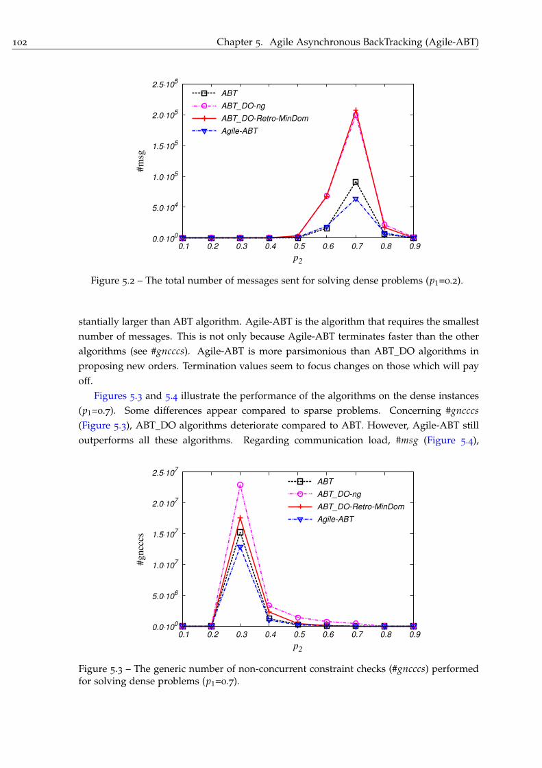
102 Chapter 5. Agile Asynchronous BackTracking (Agile-ABT)
0.0⋅100
5.0⋅104
1.0⋅105
1.5⋅105
2.0⋅105
2.5⋅105
0.1 0.2 0.3 0.4 0.5 0.6 0.7 0.8 0.9
#m
sg
p2
ABT
ABT_DO-ng
ABT_DO-Retro-MinDom
Agile-ABT
Figure 5.2 – The total number of messages sent for solving dense problems (p1=0.2).
stantially larger than ABT algorithm. Agile-ABT is the algorithm that requires the smallest
number of messages. This is not only because Agile-ABT terminates faster than the other
algorithms (see #gncccs). Agile-ABT is more parsimonious than ABT_DO algorithms in
proposing new orders. Termination values seem to focus changes on those which will pay
off.
Figures 5.3 and 5.4 illustrate the performance of the algorithms on the dense instances
(p1=0.7). Some differences appear compared to sparse problems. Concerning #gncccs
(Figure 5.3), ABT_DO algorithms deteriorate compared to ABT. However, Agile-ABT still
outperforms all these algorithms. Regarding communication load, #msg (Figure 5.4),
0.0⋅100
5.0⋅106
1.0⋅107
1.5⋅107
2.0⋅107
2.5⋅107
0.1 0.2 0.3 0.4 0.5 0.6 0.7 0.8 0.9
#gncccs
p2
ABT
ABT_DO-ng
ABT_DO-Retro-MinDom
Agile-ABT
Figure 5.3 – The generic number of non-concurrent constraint checks (#gncccs) performedfor solving dense problems (p1=0.7).

5.5. Experimental Results 103
0.0⋅100
5.0⋅106
1.0⋅107
1.5⋅107
2.0⋅107
2.5⋅107
0.1 0.2 0.3 0.4 0.5 0.6 0.7 0.8 0.9
#m
sg
p2
ABT
ABT_DO-ng
ABT_DO-Retro-MinDom
Agile-ABT
Figure 5.4 – The total number of messages sent for solving dense problems (p1=0.7).
ABT_DO-ng and ABT_DO-Retro-MinDom show the same bad performance as in sparse
problems. Agile-ABT shows similar communication load as ABT. This confirms its good
behavior observed on sparse problems.
5.5.2 Distributed Sensor Target Problems
The Distributed Sensor-Target Problem (SensorDisCSP) [Béjar et al., 2005] is a benchmark
based on a real distributed problem (see Section 1.3.2.2). It consists of n sensors that track m
targets. Each target must be tracked by 3 sensors. Each sensor can track at most one target.
A solution must satisfy visibility and compatibility constraints. The visibility constraint
defines the set of sensors to which a target is visible. The compatibility constraint defines
the compatibility among sensors. In our implementation of the DisCSP algorithms, the
encoding of the SensorDisCSP presented in Section 1.3.2.2 is translated to an equivalent
formulation where we have three virtual agents for every real agent, each virtual agent
handling a single variable.
Problems are characterized by �n, m, pc, pv�, where n is the number of sensors, m is the
number of targets, each sensor can communicate with a fraction pc of the sensors that are
in its sensing range, and each target can be tracked by a fraction pv of the sensors having
the target in their sensing range. We present results for the class � 25, 5, 0.4, pv�, where we
vary pv from 0.1 to 0.9 by steps of 0.1. Again, for each pv we generated 25 instances, solved
4 times each and averaged over the 100 runs. The results are shown in Figures 5.5 and 5.6.
When comparing the speed-up of algorithms (Figure 5.5), Agile-ABT is slightly dom-
inated by ABT and ABT_DO-ng in the interval [0.3 0.5], while outside of this interval,
Agile-ABT outperforms all the algorithms. Nonetheless, the performance of ABT and
ABT_DO-ng dramatically deteriorate in the interval [0.1 0.3]. Concerning communication
load (Figure 5.6), as opposed to other dynamic ordering algorithm, Agile-ABT is always
better than or as good as standard ABT.

104 Chapter 5. Agile Asynchronous BackTracking (Agile-ABT)
0.0⋅100
5.0⋅105
1.0⋅106
1.5⋅106
2.0⋅106
2.5⋅106
3.0⋅106
0.1 0.2 0.3 0.4 0.5 0.6 0.7 0.8 0.9
#gncccs
pv
ABT
ABT_DO-ng
ABT_DO-Retro-MinDom
Agile-ABT
Figure 5.5 – The generic number non-concurrent constraint checks performed on instanceswhere pc=0.4.
0.0⋅100
5.0⋅105
1.0⋅106
1.5⋅106
2.0⋅106
2.5⋅106
0.1 0.2 0.3 0.4 0.5 0.6 0.7 0.8 0.9
#m
sg
pv
ABT
ABT_DO-ng
ABT_DO-Retro-MinDom
Agile-ABT
Figure 5.6 – Total number of exchanged messages on instances where pc=0.4.
5.5.3 Discussion
From the experiments above we can conclude that Agile-ABT outperforms other al-
gorithms in term of computation effort (#gncccs) when solving random DisCSP problem.
On structured problems (SensorDCSP), our results suggest that Agile-ABT is more robust
than other algorithms whose performance is sensitive to the type of problems solved. Con-
cerning communication load (#msg), Agile-ABT is more robust than other versions of ABT
with dynamic agent ordering. As opposed to them, it is always better than or as good as
standard ABT on difficult problems.
At first sight, Agile-ABT seems to need less messages than other algorithms but these
messages are longer than messages sent by other algorithms. One could object that for

5.5. Experimental Results 105
0
50
100
150
200
250
0.1 0.2 0.3 0.4 0.5 0.6 0.7 0.8 0.9
longes
t m
essa
ge
size
p2
ABT
ABT_DO-ng
ABT_DO-Retro-MinDom
Agile-ABT
(a) sparse random problems (p1=0.2)
0
50
100
150
200
250
300
350
0.1 0.2 0.3 0.4 0.5 0.6 0.7 0.8 0.9
longes
t m
essa
ge
size
p2
ABT
ABT_DO-ng
ABT_DO-Retro-MinDom
Agile-ABT
(b) dense random problems (p1=0.7)
0
50
100
150
200
250
0.1 0.2 0.3 0.4 0.5 0.6 0.7 0.8 0.9
longes
t m
essa
ge
size
pv
ABT
ABT_DO-ng
ABT_DO-Retro-MinDom
Agile-ABT
(c) Sensor Target problems where pc = 0.4
Figure 5.7 – Maximum message size in bytes.
Agile-ABT, counting the number of exchanged messages is biased. However, counting
the number of exchanged messages would be biased only if #msg was smaller than the
number of physically exchanged messages (going out from the network card). Now, in our
experiments, they are the same.
The International Organization for Standardization (ISO) has designed the Open
Systems Interconnection (OSI) model to standardize networking. TCP and UDP are
the principal Transport Layer protocols using OSI model. The internet protocols IPv4
(http://tools.ietf.org/html/rfc791) and IPv6 (http://tools.ietf.org/html/rfc2460) specify
the minimum datagram size that we are guaranteed to send without fragmentation of
a message (in one physical message). This is 568 bytes for IPv4 and 1,272 bytes for
IPv6 when using either TCP or UDP (UDP is 8 bytes less than TCP, see RFC-768 –
http://tools.ietf.org/html/rfc768).
Figure 5.7 shows the size of the longest message sent by each algorithm on our random
and sensor problems. It is clear that Agile-ABT requires lengthy messages compared to

106 Chapter 5. Agile Asynchronous BackTracking (Agile-ABT)
other algorithms. However, the longest message sent is always less than 568 bytes (in the
worst case it is less than 350, see Figure 5.7(b)).
5.6 Related Works
In [Ginsberg and McAllester, 1994], Ginsberg and McAllester proposed Partial Or-
der Dynamic Backtracking (PODB), a polynomial space algorithm for centralized CSP that
attempted to address the rigidity of dynamic backtracking. The Generalized Partial Order
Dynamic Backtracking (GPODB), an algorithm that generalizes both PODB [Ginsberg and
McAllester, 1994] and the Dynamic Backtracking DBT [Ginsberg, 1993] was proposed in[Bliek, 1998]. GPODB maintains a set of ordering constraints (aka. safety conditions) on
the variables. These ordering constraints imply only a partial order on the variables. This
provides flexibility in the reordering of variables in a nogood. Agile-ABT has some simi-
larities with GPODB because Agile-ABT also maintains a set of safety conditions (induced
by explanations). However, the set of safety conditions maintained by Agile-ABT allows
more total orderings than the set of safety conditions maintained by GPODB. In addition,
whenever a new nogood is generated by GPODB, the target of this nogood must be se-
lected such that the safety conditions induced by the new nogood satisfy all existing safety
conditions. On the contrary, Agile-ABT allows discarding explanations, and thus, relaxing
some of the safety conditions. These two points give Agile-ABT more flexibility in choosing
the backtracking target.
5.7 Summary
We have proposed Agile-ABT, an algorithm that is able to change the ordering of agents
more agilely than all previous approaches. Thanks to the original concept of termination
value, Agile-ABT is able to choose a backtracking target that is not necessarily the agent
with the current lowest priority within the conflicting agents. Furthermore, the ordering of
agents appearing before the backtracking target can be changed. These interesting features
are unusual for an algorithm with polynomial space complexity. Our experiments confirm
the significance of these features.
6Corrigendum to “Min-domain
retroactive ordering for
Asynchronous Backtracking”
The asynchronous backtracking algorithm with dynamic ordering, ABT_DO, have been
proposed in [Zivan and Meisels, 2006a]. ABT_DO allows changing the order of agents
during distributed asynchronous search. In ABT_DO, when an agent assigns a value to its
variable, it can reorder lower priority agents. Retroactive heuristics called ABT_DO-Retro
which allow more flexibility in the selection of new orders were introduced in [Zivan et
al., 2009]. Unfortunately, the description of the time-stamping protocol used to compare
orders in ABT_DO-Retro may lead to an implementation in which ABT_DO-Retro may not
terminate. In this chapter, we give an example that shows how ABT_DO-Retro can enter
in an infinite loop if it uses this protocol and we propose a new correct way for comparing
time-stamps.
This chapter is organized as follows. Section 6.1 introduces the retroactive heuristics
of the asynchronous backtracking algorithm with dynamic ordering (ABT_DO-Retro). We
describe in Section 6.2 the natural understanding of the protocol used for comparing time-
stamps in ABT_DO with retroactive heuristics (ABT_DO-Retro). Section 6.3 illustrates an
example that shows, if ABT_DO-Retro uses that protocol, how it can fall into an infinite
loop. We describe the correct method for comparing time-stamps and give the proof that
our method for comparing orders is correct in Section 6.4.
6.1 Introduction
Zivan and Meisels (2006a) proposed the asynchronous backtracking algorithm with
dynamic ordering, ABT_DO, in [Zivan and Meisels, 2006a]. In ABT_DO, when an agent
assigns a value to its variable, it can reorder lower priority agents. Each agent in ABT_DO
holds a current order (that is, a vector of agent IDs) and a vector of counters (one counter
attached to each agent ID). The vector of counters attached to agent IDs forms a time-
stamp. Initially, all time-stamp counters are set to zero and all agents start with the same
107

108 Chapter 6. Corrigendum to “Min-domain retroactive ordering for Asynchronous Backtracking”
order. Each agent that proposes a new order increments its counter by one and sets to
zero counters of all lower priority agents (the counters of higher priority agents are not
modified). When comparing two orders, the strongest is the one with the lexicographically
larger time-stamp. In other words, the strongest order is the one for which the first different
counter is larger. The most successful ordering heuristic found in [Zivan and Meisels,
2006a] was the nogood-triggered heuristic in which an agent that receives a nogood moves
the nogood generator to be right after it in the order.
A new type of ordering heuristics for ABT_DO is presented in [Zivan et al., 2009].
These heuristics, called retroactive heuristics (ABT_DO-Retro), enable the generator of the
nogood to propose a new order in which it moves itself to a higher priority position than
that of the target of the backtrack. The degree of flexibility of these heuristics depends
on a parameter K. Agents that detect a dead end are moved to a higher priority position
in the order. If the length of the created nogood is larger than K, they can be moved up
to the place that is right after the second last agent in the nogood. If the length of the
created nogood is smaller than or equal to K, the sending agent can be moved to a position
before all the participants in the nogood and the nogood is sent and saved by all of the
participants in the nogood. Since agents must store nogoods that are smaller than or equal
to K, the space complexity of agents is exponential in K.
Recent attempts to implement the ABT_DO-Retro algorithm proposed in [Zivan et al.,
2009] have revealed a specific detail of the algorithm that concerns its time-stamping pro-
tocol. The natural understanding of the description given in [Zivan et al., 2009] of the
time-stamping protocol used to compare orders in ABT_DO-Retro can affect the correct-
ness of the algorithm. In this chapter we address this protocol by describing the undesired
outcome of this protocol and propose an alternative deterministic method that ensures the
outcome expected in [Zivan et al., 2009].
6.2 Background
The degree of flexibility of the retroactive heuristics mentioned above depends on a
parameter K. K defines the level of flexibility of the heuristic with respect to the amount
of information an agent can store in its memory. Agents that detect a dead end move
themselves to a higher priority position in the order. If the length of the nogood created is
not larger than K then the agent can move to any position it desires (even to the highest
priority position) and all agents that are included in the nogood are required to add the
nogood to their set of constraints and hold it until the algorithm terminates. If the size
of the created nogood is larger than K, the agent that created the nogood can move up to
the place that is right after the second last agent in the nogood. Since agents must store
nogoods that are smaller than or equal to K, the space complexity of agents is exponential
in K.
The best retroactive heuristic introduced in [Zivan et al., 2009] is called ABT_DO-Retro-
MinDom. This heuristic does not require any additional storage (i.e., K = 0). In this
heuristic, the agent that generates a nogood is placed in the new order between the last
6.2. Background 109
and the second last agents in the generated nogood. However, the generator of the nogood
moves to a higher priority position than the backtracking target (the agent the nogood
was sent to) only if its domain is smaller than that of the agents it passes on the way up.
Otherwise, the generator of the nogood is placed right after the last agent with a smaller
domain between the last and the second last agents in the nogood.
In asynchronous backtracking algorithms with dynamic ordering, agents propose new
orders asynchronously. Hence, one must enable agents to coherently decide which of
two different orders is the stronger. To this end, as it has been explained in [Zivan and
Meisels, 2006a] and recalled in [Zivan et al., 2009], each agent in ABT_DO holds a counter
vector (one counter attached to each position in the order). The counter vector and the
indexes of the agents currently in these positions form a time-stamp. Initially, all counters
are set to zero and all agents are aware of the initial order. Each agent that proposes a
new order increments the counter attached to its position in the current order and sets
to zero counters of all lower priority positions (the counters of higher priority positions
are not modified). The strongest order is determined by a lexicographic comparison of
counter vectors combined with the agent indexes. However, the rules for reordering agents
in ABT_DO imply that the strongest order is always the one for which the first different
counter is larger.
In ABT_DO-Retro agents can be moved to a position that is higher than that of the
target of the backtrack. This new feature makes it possible to generate two contradictory
orders that have the same time stamp. To address this additional issue, the description
given by the authors was limited to two sentences: “The most relevant order is determined
lexicographically. Ties which could not have been generated in standard ABT_DO, are broken using
the agents indexes” [quoted from [Zivan et al., 2009], page 190, Theorem 1].
The natural understanding of this description is that the strongest order is the one
associated with the lexicographically greater counter vector, and when the counter vec-
tors are equal the lexicographic order on the indexes of agents breaks the tie by pre-
ferring the one with smaller vector of indexes. We will refer to this natural interpre-
tation as method m1. Let us illustrate method m1 via an example. Consider two or-
ders O1=[A1, A3, A2, A4, A5] and O2=[A1, A2, A3, A4, A5] where the counter vector asso-
ciated with O1 equals V1 = [2, 4, 2, 2, 0] and the counter vector associated with O2 equals
V2 = [2, 4, 2, 1, 0]. Since in m1 the strongest order is determined by comparing lexicograph-
ically the counter vectors, in this example O1 is considered stronger than O2. In Section 6.3
of this chapter, we show that method m1 may lead ABT_DO-Retro to fall in an infinite loop
when K = 0.
The right way to compare orders is to compare their counter vectors, one position at
a time from left to right, until they differ on a position (preferring the order with greater
counter) or they are equal on that position but the indexes of the agents in that position
differ (preferring the smaller index). We will refer to this method as m2. Consider again
the two orders O1 and O2 and associated counter vectors defined above. The counter at
the first position equals 2 on both counter vectors and the index of the first agent in O1
(i.e., A1) is the same as in O2, the counter at the second position equals 4 on both counter
vectors,however the index of the second agent in O2 (i.e., A2) is smaller than the index of
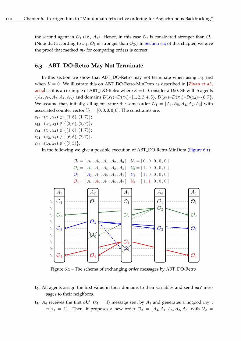
110 Chapter 6. Corrigendum to “Min-domain retroactive ordering for Asynchronous Backtracking”
the second agent in O1 (i.e., A3). Hence, in this case O2 is considered stronger than O1.
(Note that according to m1, O1 is stronger than O2.) In Section 6.4 of this chapter, we give
the proof that method m2 for comparing orders is correct.
6.3 ABT_DO-Retro May Not Terminate
In this section we show that ABT_DO-Retro may not terminate when using m1 and
when K = 0. We illustrate this on ABT_DO-Retro-MinDom as described in [Zivan et al.,
2009] as it is an example of ABT_DO-Retro where K = 0. Consider a DisCSP with 5 agents
{A1, A2, A3, A4, A5} and domains D(x1)=D(x5)={1, 2, 3, 4, 5}, D(x2)=D(x3)=D(x4)={6, 7}.
We assume that, initially, all agents store the same order O1 = [A1, A5, A4, A2, A3] with
associated counter vector V1 = [0, 0, 0, 0, 0]. The constraints are:
c12 : (x1, x2) �∈ {(1, 6), (1, 7)};
c13 : (x1, x3) �∈ {(2, 6), (2, 7)};
c14 : (x1, x4) �∈ {(1, 6), (1, 7)};
c24 : (x2, x4) �∈ {(6, 6), (7, 7)}.
c35 : (x3, x5) �∈ {(7, 5)}.
In the following we give a possible execution of ABT_DO-Retro-MinDom (Figure 6.1).
O1 = [ A1 , A5 , A4 , A2 , A3 ] V1 = [ 0 , 0 , 0 , 0 , 0 ]
O2 = [ A4 , A1 , A5 , A2 , A3 ] V2 = [ 1 , 0 , 0 , 0 , 0 ]
O3 = [ A2 , A1 , A5 , A4 , A3 ] V3 = [ 1 , 0 , 0 , 0 , 0 ]
O4 = [ A4 , A3 , A1 , A5 , A2 ] V4 = [ 1 , 1 , 0 , 0 , 0 ]
t0
t1
t2
t3
t4
t5
t6
t7
t8
A1
O1
O2
O3
O4
A2
O1
O3
O2
O4
A3
O1
O2
O4
O3
A4
O1
O2
O3
A5
O1
O2
O3
O4
Figure 6.1 – The schema of exchanging order messages by ABT_DO-Retro
t0: All agents assign the first value in their domains to their variables and send ok? mes-
sages to their neighbors.
t1: A4 receives the first ok? (x1 = 1) message sent by A1 and generates a nogood ng1 :
¬(x1 = 1). Then, it proposes a new order O2 = [A4, A1, A5, A2, A3] with V2 =

6.3. ABT_DO-Retro May Not Terminate 111
[1, 0, 0, 0, 0]. Afterwards, it assigns the value 6 to its variable and sends ok? (x4 = 6)
message to all its neighbors (including A2).
t2: A3 receives O2 = [A4, A1, A5, A2, A3] and deletes O1 since O2 is stronger; A1 receives
the nogood sent by A4, it replaces its assignment to 2 and sends an ok? (x1 = 2)
message to all its neighbors.
t3: A2 has not yet received O2 and the new assignment of A1. A2 generates a new nogood
ng2 : ¬(x1 = 1) and proposes a new order O3 = [A2, A1, A5, A4, A3] with V3 =
[1, 0, 0, 0, 0]; Afterwards, it assigns the value 6 to its variable and sends ok? (x2 = 6)
message to all its neighbors (including A4).
t4: A4 receives the new assignment of A2 (i.e., x2 = 6) and O3 = [A2, A1, A5, A4, A3].
Afterwards, it discards O2 since O3 is stronger; Then, A4 tries to satisfy c24 because
A2 has a higher priority according to O3. Hence, A4 replaces its current assignment
(i.e., x4 = 6) by x4 = 7 and sends an ok? (x4 = 7) message to all its neighbors
(including A2).
t5: When receiving O2, A2 discards it because its current order is stronger;
t6: After receiving the new assignment of A1 (i.e., x1 = 2) and before receiving O3 =
[A2, A1, A5, A4, A3], A3 generates a nogood ng3 : ¬(x1 = 2) and proposes a new order
O4 = [A4, A3, A1, A5, A2] with V4 = [1, 1, 0, 0, 0]; The order O4 is stronger according
to m1 than O3. Since in ABT_DO, an agent sends the new order only to lower priority
agents, A3 will not send O4 to A4 because it is a higher priority agent.
t7: A3 receives O3 and then discards it because it is obsolete;
t8: A2 receives O4 but it has not yet received the new assignment of A4. Then, it tries to
satisfy c24 because A4 has a higher priority according to its current order O4. Hence,
A2 replaces its current assignment (i.e., x2 = 6) by x2 = 7 and sends an ok? (x2 = 7)
message to all its neighbors (including A4).
t9: A2 receives the ok? (x4 = 7) message sent by A4 in t4 and changes its current value
(i.e., x2 = 7) by x2 = 6. Then, A2 sends an ok? (x2 = 6) message to all its neighbors
(including A4). At the same time, A4 receives ok? (x2 = 7) sent by A2 in t8. A4
changes its current value (i.e., x4 = 7) by x4 = 6. Then, A4 sends an ok? (x4 = 6)
message to all its neighbors (including A2).
t10: A2 receives the ok? (x4 = 6) message sent by A4 in t9 and changes its current value
(i.e., x2 = 6) by x2 = 7. Then, A2 sends an ok? (x2 = 7) message to all its neighbors
(including A4). At the same moment, A4 receives ok? (x2 = 6) sent by A2 in t9. A4
changes its current value (i.e., x4 = 6) by x4 = 7. Then, A4 sends an ok? (x4 = 7)
message to all its neighbors (including A2).
t11: We come back to the situation we were facing at time t9, and therefore ABT_DO-Retro-
MinDom may fall in an infinite loop when using method m1.

112 Chapter 6. Corrigendum to “Min-domain retroactive ordering for Asynchronous Backtracking”
6.4 The Right Way to Compare Orders
Let us formally define the second method, m2, for comparing orders in which we com-
pare the indexes of agents as soon as the counters in a position are equal on both counter
vectors associated with the orders being compared. Given any order O, we denote by
O(i) the index of the agent located in the ith position in O and by V(i) the counter in
the ith position in the counter vector V associated to order O. An order O1 with counter
vector V1 is stronger than an order O2 with counter vector V2 if and only if there exists a
position i, 1 ≤ i ≤ n, such that for all 1 ≤ j < i, V1(j) = V2(j) and O1(j) = O2(j), and
V1(i) > V2(i) or V1(i) = V2(i) and O1(i) < O1(i).
In our correctness proof for the use of m2 in ABT_DO-Retro we use the following no-
tations. The initial order known by all agents is denoted by Oinit. Each agent, Ai, stores a
current order, Oi, with an associated counter vector, Vi. Each counter vector Vi consists of
n counters Vi(1), . . . , Vi(n) such that Vi = [Vi(1), . . . , Vi(n)]. When Vi is the counter
vector associated with an order Oi, we denote by Vi(k) the value of the kth counter in the
counter vector stored by the agent Ai. We define ρ to be equal to max{Vi(1) | i ∈ 1..n}.
The value of ρ evolves during the search so that it always corresponds to the value of the
largest counter among all the first counters stored by agents.
Let K be the parameter defining the degree of flexibility of the retroactive heuristics
(see Section 6.1). Next we show that the ABT_DO-Retro algorithm is correct when using
m2 and with K = 0. The proof that the algorithm is correct when K �= 0 can be found in[Zivan et al., 2009].
To prove the correctness of ABT_DO-Retro we use induction on the number of agents.
For a single agent the order is static therefore the correctness of standard ABT implies the
correctness of ABT_DO-Retro. Assume ABT_DO-Retro is correct for every DisCSP with
n − 1 agents. We show in the following that ABT_DO-Retro is correct for every DisCSP
with n agents. To this end we first prove the following lemmas.
Lemma 6.1. Given enough time, if the value of ρ does not change, the highest priority agent
in all orders stored by all agents will be the same.
Proof. Assume the system reaches a state σ where the value of ρ no longer increases. Let Oi
be the order that, when generated, caused the system to enter state σ. Inevitably, we have
Vi(1) = ρ. Assume that Oi �= Oinit and let Ai be the agent that generated Oi. The agent Ai
is necessarily the highest priority agent in the new order Oi because, the only possibility for
the generator of a new order to change the position of the highest priority agent is to put
itself in the first position in the new order. Thus, Oi is sent by Ai to all other agents because
Ai must send Oi to all agents that have a lower priority than itself. So after a finite time all
agents will be aware of Oi. This is also true if Oi = Oinit. Now, by assumption the value of
ρ no longer increases. As a result, the only way for another agent to generate an order O�
such that the highest priority agents in Oi and O� are different (i.e., O�(1) �= Oi(1)) is to
put itself in first position in O� and to do that before it has received Oi (otherwise O� would
increase ρ). Therefore, the time passed from the moment the system entered state σ until a
new order O� was generated is finite. Let O j be the strongest such order (i.e., O�) and let

6.4. The Right Way to Compare Orders 113
Aj be the agent that generated O j. That is, Aj is the agent with smallest index among those
who generated such an order O�. The agent Aj will send O j to all other agents and O j will
be accepted by all other agents after a finite amount of time. Once an agent has accepted
O j, all orders that may be generated by this agent do not reorder the highest priority agent
otherwise ρ would increase.
Lemma 6.2. If the algorithm is correct for n − 1 agents then it terminates for n agents.
Proof. If during the search ρ continues to increase, this means that some of the agents
continue to send new orders in which they put themselves in first position. Hence, the
nogoods they generate when proposing the new orders are necessarily unary (i.e., they
have an empty left-hand side) because in ABT_DO-Retro, when the parameter K is zero
the nogood sender cannot put itself in a higher priority position than the second last in the
nogood. Suppose ng0 = ¬(xi = vi) is one of these nogoods, sent by an agent Aj. After a
finite amount of time, agent Ai, the owner of xi, will receive ng0. Three cases can occur.
First case, Ai still has value vi in its domain. So the value vi is pruned once and for all
from D(xi) thanks to ng0. Second case, Ai has already received a nogood equivalent to ng0
from another agent. Here, vi no longer belongs to D(xi). When changing its value, Ai has
sent an ok? message with its new value v�i. If Ai and Aj were neighbors, this ok? message
has been sent to Aj. If Ai and Aj were not neighbors when Ai changed its value to v�i, this
ok? message was sent by Ai to Aj after Aj requested to add a link between them at the
moment it generated ng0. Thanks to the assumption that messages are always delivered
in a finite amount of time, we know that Aj will receive the ok? message containing
v�i a finite amount of time after it sent ng0. Thus, Aj will not be able to send forever
nogoods about a value vi pruned once and for all from D(xi). Third case, Ai already
stores a nogood with a non empty left-hand side discarding vi. Notice that although Aj
moves to the highest priority position, Ai may be of lower priority, i.e., there can be agents
with higher priority than Ai according to the current order that are not included in ng0.
Thanks to the standard highest possible lowest variable involved [Hirayama and Yokoo, 2000;
Bessiere et al., 2005] heuristic for selecting nogoods in ABT algorithms, we are guaranteed
that the nogood with empty left-hand side ng0 will replace the other existing nogood and vi
will be permanently pruned from D(xi). Thus, in all three cases, every time ρ increases, we
know that an agent has moved to the first position in the order, and a value was definitively
pruned a finite amount of time before or after. There is a bounded number of values in
the network. Thus, ρ cannot increase forever. Now, if ρ stops increasing, then after a finite
amount of time the highest priority agent in all orders stored by all agents will be the same
(Lemma 6.1). Since the algorithm is correct for n − 1 agents, after each assignment of the
highest priority agent, the rest of the agents will either reach an idle state, 1 generate an
empty nogood indicating that there is no solution, or generate a unary nogood, which is
sent to the highest priority agent. Since the number of values in the system is finite, the
third option, which is the only one that does not imply immediate termination, cannot
occur forever.
1. As proved in Lemma 6.3, this indicates that a solution was found.

114 Chapter 6. Corrigendum to “Min-domain retroactive ordering for Asynchronous Backtracking”
Lemma 6.3. If the algorithm is correct for n − 1 agents then it is sound for n agents.
Proof. Let O� be the strongest order generated before reaching the state of quiescence and
let O be the strongest order generated such that V(1) = V �(1) (and such that O has
changed the position of the first agent –assuming O �= Oinit). Given the rules for reordering
agents, the agent that generated O has necessarily put himself first because it has modified
V(1) and thus also the position of the highest agent. So it has sent O to all other agents.
When reaching the state of quiescence, we know that no order Oj with Oj(1) �= O(1)
has been generated because this would break the assumption that O is the strongest order
where the position of the first agent has been changed. Hence, at the state of quiescence,
every agent Ai stores an order Oi such that Oi(1) = O(1). (This is also true if O = Oinit.)
Let us consider the DisCSP P composed of the n − 1 lower priority agents according to O.
Since the algorithm is correct for n − 1 agents, the state of quiescence means that a solution
was found for P. Also, since all agents in P are aware that O(1) is the agent with the
highest priority, the state of quiescence also implies that all constraints that involve O(1)
have been successfully tested by agents in P, otherwise at least one agent in P would try
to change its value and send an ok? or ngd message. Therefore, the state of quiescence
implies that a solution was found.
Lemma 6.4. The algorithm is complete
Proof. All nogoods are generated by logical inferences from existing constraints. Thus, an
empty nogood cannot be inferred if a solution exists.
Following Lemma 6.2, 6.3 and 6.4 we obtain the correctness of the main theorem in this
chapter.
Theorem 6.1. The ABT_DO-Retro algorithm with K = 0 is correct when using the m2 method for
selecting the strongest order.
6.5 Summary
We proposed in this chapter a corrigendum of the protocol designed for establishing
the priority between orders in the asynchronous backtracking algorithm with dynamic or-
dering using retroactive heuristics (ABT_DO-Retro). We presented an example that shows
how ABT_DO-Retro can enter an infinite loop following the natural understanding of the
description given by the authors of ABT_DO-Retro. We described the correct way for com-
paring time-stamps of orders. We gave the proof that our method for comparing orders is
correct.

7DisChoco 2.0
Distributed constraint reasoning is a powerful concept to model and solve naturally
distributed constraint satisfaction/optimization problems. However, there are very
few open-source tools dedicated to solve such problems: DisChoco, DCOPolis and FRODO.
A distributed constraint reasoning platform must have some important features: It should
be reliable and modular in order to be easy to personalize and extend, be independent
of the communication system, allow the simulation of agents on a single virtual machine,
make it easy for deployment on a real distributed framework, and allow agents with a local
complex problems. This paper presents DisChoco 2.0, a complete redesign of the DisChoco
platform that guarantees these features and that can deal both with distributed constraint
satisfaction problems and with distributed constraint optimization problems.
This chapter is organized as follows. Section 7.2 presents the global architecture of
DisChoco 2.0. In Section 7.3, we show how a user can define her problem and solve it
using the DisChoco 2.0 platform. Section 7.4 shows the different benchmarks available in
DisChoco and how researchers in the DCR field can use them for evaluating algorithms
performance. We conclude the paper in Section 7.5.
7.1 Introduction
Distributed Constraint Reasoning (DCR) is a framework for solving various problems
arising in Distributed Artificial Intelligence. In DCR, a problem is expressed as a Dis-
tributed Constraint Network (DCN). A DCN is composed of a group of autonomous agents
where each agent has control of some elements of information about the problem, that is,
variables and constraints. Each agent own its local constraint network. Variables in differ-
ent agents are connected by constraints. Agents try to find a local solution (locally consis-
tent assignment) and communicate it with other agents using a DCR protocol to check its
consistency against constraints with variables owned by other agents [Yokoo et al., 1998;
Yokoo, 2000a].
A DCN offers an elegant way for modeling many everyday combinatorial problems
that are distributed by nature (e.g., distributed resource allocation [Petcu and Faltings,
2004], distributed meeting scheduling [Wallace and Freuder, 2002], sensor networks [Bé-
jar et al., 2005]). Several algorithms for solving this kind of problems have been devel-
115
116 Chapter 7. DisChoco 2.0
oped. Asynchronous Backtracking (ABT [Yokoo et al., 1992], ABT-Family [Bessiere et al.,
2005]), Asynchronous Forward Checking (AFC) [Meisels and Zivan, 2007] and Nogood-
based Asynchronous Forward-Checking (AFC-ng) [Wahbi et al., 2012] were developed
to solve Distributed Constraint Satisfaction Problems (DisCSP). Asynchronous Distributed
constraints OPTimization (Adopt) [Modi et al., 2005], Asynchronous Forward-Bounding
(AFB) [Gershman et al., 2009], Asynchronous Branch-and-Bound (Adopt-BnB) [Yeoh et
al., 2008] and Dynamic backtracking for distributed constraint optimization (DyBop) [Ez-
zahir et al., 2008a] were developed to solve Distributed Constraint Optimization Problems
(DCOP).
Programming DCR algorithms is a difficult task because the programmer must ex-
plicitly juggle between many very different concerns, including centralized programming,
parallel programming, asynchronous and concurrent management of distributed structures
and others. In addition, there are very few open-source tools for solving DCR problems:
DisChoco, DCOPolis [Sultanik et al., 2008] and FRODO [Léauté et al., 2009]. Researchers
in DCR are concerned with developing new algorithms, and comparing their performance
with existing algorithms. Open-source platforms are essential tools to integrate and test
new ideas without having the burden to reimplement from scratch an ad-hoc solver. For
this reason a DCR platform should have the following features:
• be reliable and modular, so it is easy to personalize and extend;
• be independent from the communication system;
• allow the simulation of multi-agent systems on a single machine;
• make it easy to implement a real distributed framework;
• allow the design of agents with local constraint networks.
In this paper we present DisChoco 2.0, 1 a completely redesigned platform that guar-
antees the features above. DisChoco 2.0 allows to represent both DisCSPs and DCOPs, as
opposed to other platforms. DisChoco 2.0 is not a distributed version of the centralized
solver Choco, but it implements a model to solve DCN with local complex problems (i.e.,
several variables per agent) by using Choco 2 as local solver to each agent. DisChoco 2.0 is
an open source Java library which aims at implementing DCR algorithms from an abstract
model of agent (already implemented in DisChoco). A single implementation of a DCR
algorithm can run as simulation on a single machine, or on a network of machines that
are connected via the Internet or via a wireless ad-hoc network, or even on mobile phones
compatible with J2ME.
7.2 Architecture
In order to reduce the time of development and therefore the cost of the design we
choose a components approach allowing pre-developed components to be reused. This
components approach is based on two principles:
• Each component is developed independently;
• An application is an assemblage of particular components.
1. http://www.lirmm.fr/coconut/dischoco/2. http://choco.emn.fr/
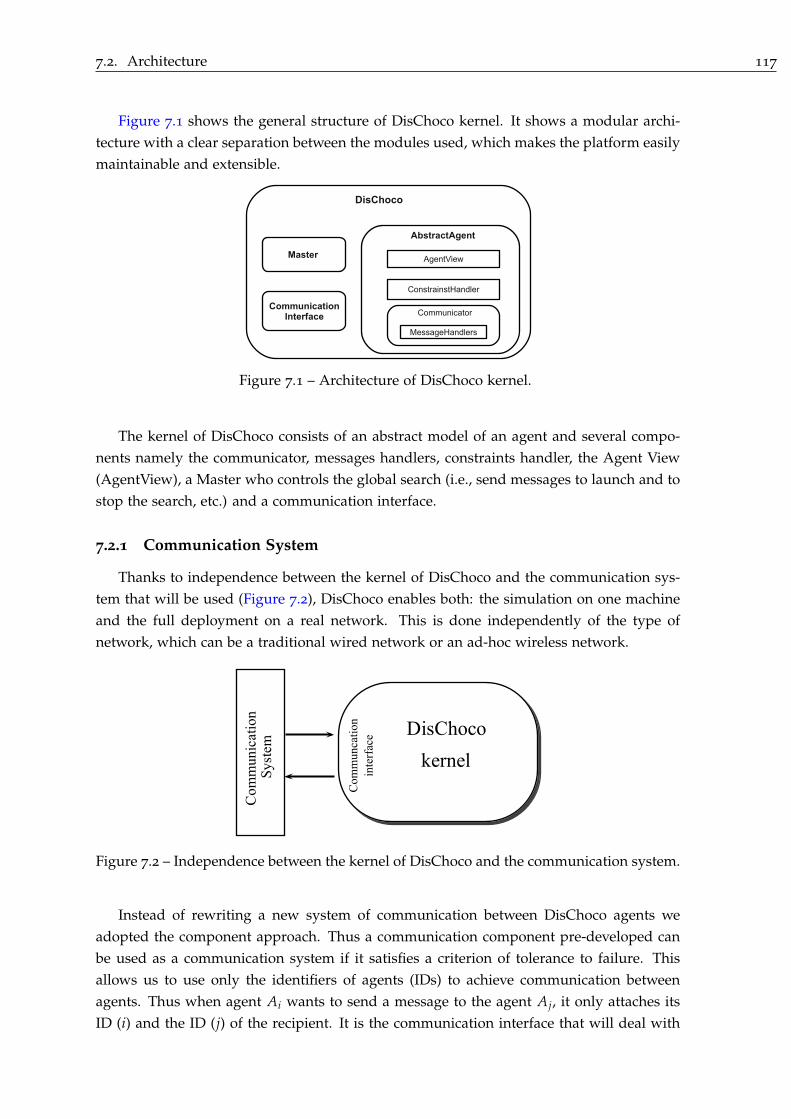
7.2. Architecture 117
Figure 7.1 shows the general structure of DisChoco kernel. It shows a modular archi-
tecture with a clear separation between the modules used, which makes the platform easily
maintainable and extensible.
!"#$%&'$!()*$
!"#$%&'#(
)*$+%,-'$+%.-$/0#,
)*112$'3-%*,
4#++-"#.-$/0#,+
+&#$)%
,-../*0'&$0-*1*$)%2&')
30#,4-'-
Figure 7.1 – Architecture of DisChoco kernel.
The kernel of DisChoco consists of an abstract model of an agent and several compo-
nents namely the communicator, messages handlers, constraints handler, the Agent View
(AgentView), a Master who controls the global search (i.e., send messages to launch and to
stop the search, etc.) and a communication interface.
7.2.1 Communication System
Thanks to independence between the kernel of DisChoco and the communication sys-
tem that will be used (Figure 7.2), DisChoco enables both: the simulation on one machine
and the full deployment on a real network. This is done independently of the type of
network, which can be a traditional wired network or an ad-hoc wireless network.
Figure 7.2 – Independence between the kernel of DisChoco and the communication system.
Instead of rewriting a new system of communication between DisChoco agents we
adopted the component approach. Thus a communication component pre-developed can
be used as a communication system if it satisfies a criterion of tolerance to failure. This
allows us to use only the identifiers of agents (IDs) to achieve communication between
agents. Thus when agent Ai wants to send a message to the agent Aj, it only attaches its
ID (i) and the ID (j) of the recipient. It is the communication interface that will deal with
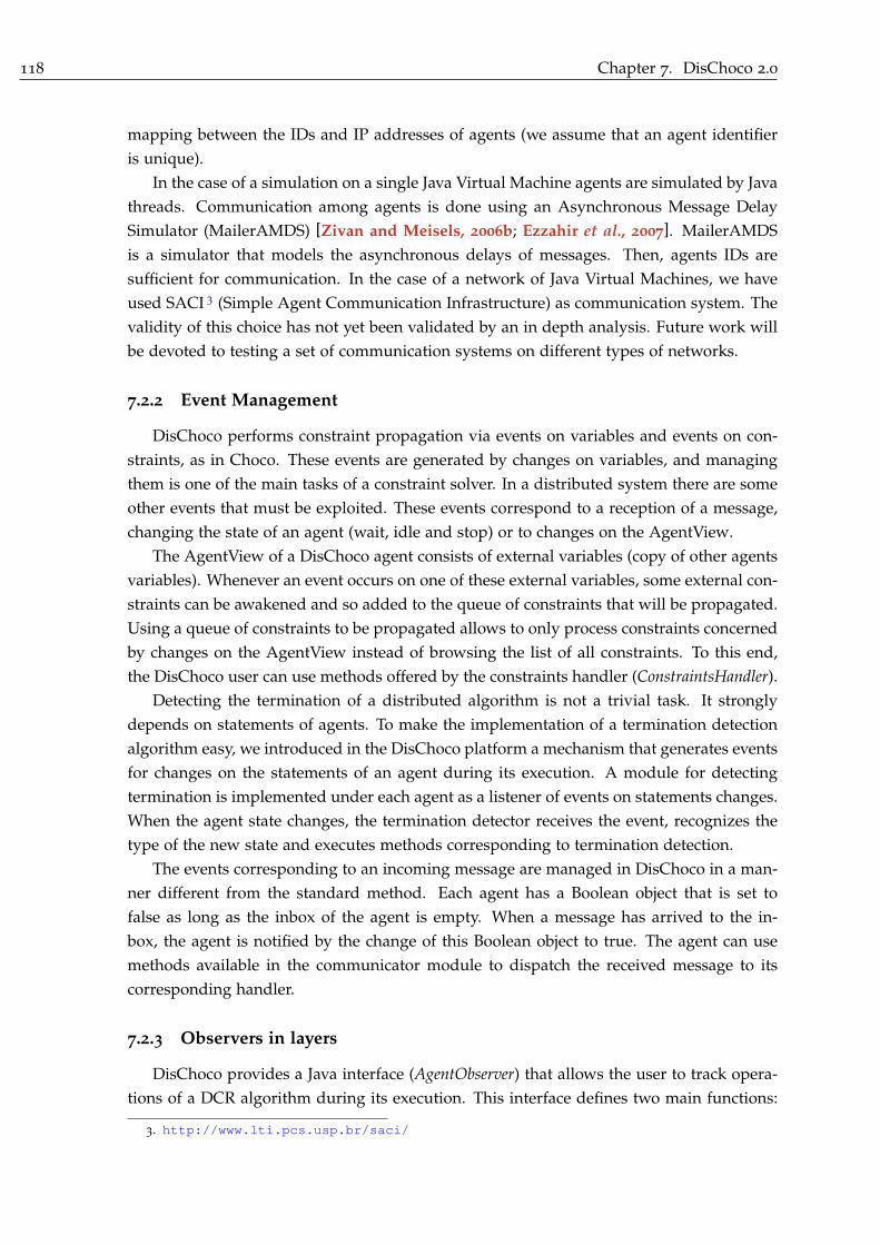
118 Chapter 7. DisChoco 2.0
mapping between the IDs and IP addresses of agents (we assume that an agent identifier
is unique).
In the case of a simulation on a single Java Virtual Machine agents are simulated by Java
threads. Communication among agents is done using an Asynchronous Message Delay
Simulator (MailerAMDS) [Zivan and Meisels, 2006b; Ezzahir et al., 2007]. MailerAMDS
is a simulator that models the asynchronous delays of messages. Then, agents IDs are
sufficient for communication. In the case of a network of Java Virtual Machines, we have
used SACI 3 (Simple Agent Communication Infrastructure) as communication system. The
validity of this choice has not yet been validated by an in depth analysis. Future work will
be devoted to testing a set of communication systems on different types of networks.
7.2.2 Event Management
DisChoco performs constraint propagation via events on variables and events on con-
straints, as in Choco. These events are generated by changes on variables, and managing
them is one of the main tasks of a constraint solver. In a distributed system there are some
other events that must be exploited. These events correspond to a reception of a message,
changing the state of an agent (wait, idle and stop) or to changes on the AgentView.
The AgentView of a DisChoco agent consists of external variables (copy of other agents
variables). Whenever an event occurs on one of these external variables, some external con-
straints can be awakened and so added to the queue of constraints that will be propagated.
Using a queue of constraints to be propagated allows to only process constraints concerned
by changes on the AgentView instead of browsing the list of all constraints. To this end,
the DisChoco user can use methods offered by the constraints handler (ConstraintsHandler).
Detecting the termination of a distributed algorithm is not a trivial task. It strongly
depends on statements of agents. To make the implementation of a termination detection
algorithm easy, we introduced in the DisChoco platform a mechanism that generates events
for changes on the statements of an agent during its execution. A module for detecting
termination is implemented under each agent as a listener of events on statements changes.
When the agent state changes, the termination detector receives the event, recognizes the
type of the new state and executes methods corresponding to termination detection.
The events corresponding to an incoming message are managed in DisChoco in a man-
ner different from the standard method. Each agent has a Boolean object that is set to
false as long as the inbox of the agent is empty. When a message has arrived to the in-
box, the agent is notified by the change of this Boolean object to true. The agent can use
methods available in the communicator module to dispatch the received message to its
corresponding handler.
7.2.3 Observers in layers
DisChoco provides a Java interface (AgentObserver) that allows the user to track opera-
tions of a DCR algorithm during its execution. This interface defines two main functions:
3. http://www.lti.pcs.usp.br/saci/

7.3. Using DisChoco 2.0 119
AbstractAgent
AgentObserver
(a) AgentObserver implemented as Layer
AbstractAgent
NCCCsObserver MSGsObserver
(b) Metrics implemented as observers
Figure 7.3 – Layer model for observers.
whenSendMessage and whenReceivedMessage. The class AbstractAgent provides a list of ob-
servers and functions to add one or several observers. Thus, when we want to implement
an application using DisChoco, we can use AgentObserver to develop a specific observer.
This model is shown in Figure 7.3(a).
When developing new algorithms, an important task is to compare their performance
to other existing algorithms. There are several metrics for measuring performance of DCR
algorithms: non-concurrent constraint checks (#ncccs [Meisels et al., 2002]), equivalent
non-concurrent constraint checks (#encccs [Chechetka and Sycara, 2006]), number of ex-
changed messages (#msg [Lynch, 1997]), degree of privacy loss[Brito et al., 2009], etc.
DisChoco simply uses AgentObserver to implement these metrics as shown in Figure 7.3(b).
The user can enable metrics when she needs them or disable some or all these metrics. The
user can develop her specific metric or her methods for collecting statistics by implement-
ing AgentObserver.
7.3 Using DisChoco 2.0
Figure 7.4 presents a definition of a distributed problem named (Hello DisChoco) using
the Java code. In this problem there are 3 agents A = {A1, A2, A3} where each agent
controls exactly one variable. The domain of A1 and A2 contains two values D1 = D2 =
{1, 2} and that of A3 contains one value D3 = {2}. There are two constraints of difference:
the first constraint is between A1 and A2 and the second one is between A2 and A3. After
defining our problem we can configure our solver. Thus, the problem can be solved using
a specified implemented protocol (ABT for example).
For DisChoco inputs we choose to use a XML format called XDisCSP derived from the
famous format XCSP 2.1. 4 Figure 7.5 shows an example of representation of the problem
defined above in the XDisCSP format. Each variable has a unique ID, which is the concate-
nation of the ID of it owner agent and index of the variable in the agent. This is necessary
when defining constraints (scope of constraints). For constraints, we used two types of con-
straints: TKC for Totally Known Constraint and PKC for Partially Known Constraint [Brito
et al., 2009]. Constraints can be defined in extension or as a Boolean function. Different
types of constraints are predefined: equal to eq(x, y), different from ne(x, y), greater than
or equal ge(x, y), greater than gt(x, y), less than or equal le(x, y), less than lt(x, y),etc.
According to this format we can model DisCSPs and DCOPs. Once a distributed con-
4. http://www.cril.univ-artois.fr/~lecoutre/benchmarks.html

120 Chapter 7. DisChoco 2.0
1 AbstractMaster master = Protocols.getMaster(Protocols.ABT);
2 DisProblem disCSP = new DisProblem("Hello DisChoco", master);
3 SimpleAgent[] agents = new SimpleAgent[3];
4 IntVar[] variables = new IntVar[3];
5 // Make agents
6 agents[0] = (SimpleAgent) disCSP.makeAgent("A1", "");
7 agents[1] = (SimpleAgent) disCSP.makeAgent("A2", "");
8 agents[2] = (SimpleAgent) disCSP.makeAgent("A3", "");
9 // Make one single variable for each agent
10 variables[0] = agents[0].makeInternalVar(new int[] {1, 2}); // x1
11 variables[1] = agents[1].makeInternalVar(new int[] {1, 2}); // x2
12 variables[2] = agents[2].makeInternalVar(new int[] {2}); // x3
13 // Make two constraints, we must to create external var on each agent
14 // But each agent must known its constraints
15 // x1!=x2
16 agents[0].neqY(agents[0].makeExternalVar(variables[1]));
17 agents[1].neqY(agents[1].makeExternalVar(variables[0]));
18 // x2!=x3
19 agents[1].neqY(agents[1].makeExternalVar(variables[2]));
20 agents[2].neqY(agents[2].makeExternalVar(variables[1]));
21 // Make a simulator to resolve the problem
22 DisCPSolver solver = new DisSolverSimulator(disCSP);
23 solver.setCentralizedAO(new LexicographicAO());
24 solver.addNCCCMetric();
25 solver.addCommunicationMetric();
26 solver.solve();
27 System.o u t.println("Problem : " + disCSP.getProblemName());
28 System.o u t.println("Solution of the problem using " + disCSP.master.getClass());
29 System.o u t.println("---------------------------------------------------------");
30 System.o u t.println(solver.getGlobalSolution());
31 System.o u t.println("---------------------------------------------------------");
32 System.o u t.println("Statistics :");
33 System.o u t.println(solver.getStatistics());
Figure 7.4 – Definition of a distributed problem using Java code.
1 <instance>2 <presentation name="Hello DisChoco" model="Simple" maxConstraintArity="2" format="XDisCSP 1.0" />
3 <agents nbAgents="3">4 <agent name="A1" id="1" description="Agent 1" />5 <agent name="A2" id="2" description="Agent 2" />
6 <agent name="A3" id="3" description="Agent 3" />7 </agents>
8 <domains nbDomains="2">9 <domain name="D1" nbValues="2">1 2</domain>
10 <domain name="D2" nbValues="1">2</domain>
11 </domains>12 <variables nbVariables="3">
13 <variable agent="A1" name="X1.0" id="0" domain="D1" description="Variable x_1" />14 <variable agent="A2" name="X2.0" id="0" domain="D1" description="Variable x_2" />
15 <variable agent="A3" name="X3.0" id="0" domain="D2" description="Variable x_3" />16 </variables>17 <predicates nbPredicates="1">
18 <predicate name="P0">19 <parameters>int x int y</parameters>
20 <expression>21 <functional>ne(x,y)</functional>22 </expression>
23 </predicate>24 </predicates>
25 <constraints nbConstraints="2">26 <constraint name="C1" model="TKC" arity="2" scope="X1.0 X2.0" reference="P0">
27 <parameters>X1.0 X2.0</parameters>28 </constraint>29 <constraint name="C2" model="TKC" arity="2" scope="X2.0 X3.0" reference="P0">
30 <parameters>X2.0 X3.0</parameters>31 </constraint>
32 </constraints>33 </instance>
Figure 7.5 – Definition of the Hello DisChoco problem in XDisCSP 1.0 format.

7.4. Experimentations 121
straint network problem is expressed in the XDisCSP format, we can solve it using one
of the protocols developed on the platform. The algorithms currently implemented in
DisChoco 2.0 are: ABT [Yokoo et al., 1992; Bessiere et al., 2005], ABT-Hyb [Brito and
Meseguer, 2004], ABT-dac [Brito and Meseguer, 2008], AFC [Meisels and Zivan, 2007],
AFC-ng [Ezzahir et al., 2009], AFC-tree [Wahbi et al., 2012], DBA [Yokoo and Hirayama,
1995] and DisFC [Brito et al., 2009] in the class of DisCSPs with simple agents. In the
class of DisCSPs where agents have local complex problems, ABT-cf [Ezzahir et al., 2008b]
was implemented. For DCOPs, the algorithms that are implemented in DisChoco 2.0 are:
Adopt [Modi et al., 2005], BnB-Adopt [Yeoh et al., 2008] and AFB [Gershman et al., 2009].
For solving a problem, we can use a simple command line:
1 java -cp dischoco.jar dischoco.simulation.Run protocol problem.xml
The Graphical User Interface (GUI) of DisChoco allows to visualize the constraint
graph. Hence, the user can analyses the structure of the problem to be solved. This also
helps to debug the algorithms. An example of the visualization is shown in Figure 7.6.
Figure 7.6 – Visualization of the structure of the distributed constraint graph.
7.4 Experimentations
In addition to its good properties (reliable and modular), DisChoco provides several
other facilities, especially for performing experimentation. The first facility is in the gen-
eration of benchmark problems. DisChoco offers a library of generators for distributed
constraint satisfaction/optimization problems (e.g., random binary DisCSPs using model
B, random binary DisCSPs with complex local problems, distributed graph coloring, dis-
tributed meeting scheduling, sensor networks, distributed N-queens, etc. These generators

122 Chapter 7. DisChoco 2.0
allow the user to test her algorithms on various types of problems ranging from purely
random problems to real world problems.
Figure 7.7 – A screenshot of the graphical user interface showing generators in DisChoco.
DisChoco is equipped with a GUI for manipulating all above generators. A screenshot
of the GUI of DisChoco shows various generators implemented on DisChoco (Figure 7.7).
Once the instances have been generated, a XML configuration file is created to collect the
instances. The generated instances are organized in a specific manner for each kind of
problems generator in a directory indicated by the user. The configuration file can also
contain details related to the configuration of the communicator and the list of algorithms
to be compared. It will be used for launching experiments. After all these configurations
have been set, the user can launch the experiments either on the GUI mode or on the
command mode.
0.0⋅100
2.0⋅105
4.0⋅105
6.0⋅105
8.0⋅105
1.0⋅106
1.2⋅106
0.1 0.2 0.3 0.4 0.5 0.6 0.7 0.8 0.9
#m
sg
p2
ABT
AFC
AFC-ng
AFC-tree
Figure 7.8 – Total number of exchanged messages on dense graph �n=20, d=10, p1=0.7, p2�.
7.5. Conclusion 123
DisChoco is also equipped with a complete manager of results. The user does not have
to worry about organizing and plotting results. All this is offered by DisChoco that auto-
matically generates gnuplot plots of the requested measures. The user can also handle all
results and compare algorithms using the GUI of DisChoco. Figure 7.8 shows an example
of plot generated from experimentations on some algorithms implemented in DisChoco.
7.5 Conclusion
In this chapter, we have presented the new version 2.0 of the DisChoco platform for
solving DCR problems. This version contains several interesting features: it is reliable and
modular, it is easy to personalize and to extend, it is independent from the communication
system and allows a deployment in a real distributed system as well as the simulation on
a single Java Virtual Machine.

Conclusions and perspectives
In this thesis, we have addressed the Distributed Constraint Satisfaction Problem
(DisCSP) framework. We proposed several complete distributed search algorithms and
reordering heuristics for DisCSPs. We have given a complete evaluation of the efficiency of
our contributions against the existing approaches in literature. Our results show that they
improve the current state-of-the-art.
Once we defined the constraint satisfaction problem formalism (CSP) and presented
some examples of academical and real combinatorial problems that can be modeled as
CSP, we reported the main existent algorithms and heuristics used for solving CSPs. Next,
we formally defined the distributed constraint satisfaction problem (DisCSP) paradigm.
We have illustrated how some instances of real world applications in multi-agent coordi-
nation can be encoded in DisCSP. We introduced the meeting scheduling problem in its
distributed form where agents may solve the problem, thanks to the DisCSP, without de-
livering their personal information to a centralized agent. We described a real distributed
resource allocation application, that is, the distributed sensor network problem, and for-
malize it as a distributed CSP. These two problems have been used as benchmarks when
comparing the algorithms proposed in this thesis. We have also described the state of the
art algorithms and heuristics for solving DisCSP.
Numerous contributions have been proposed in this thesis. Our first contribution is the
Nogood-Based Asynchronous Forward Checking (AFC-ng). AFC-ng is an algorithm based
on Asynchronous Forward Checking (AFC). AFC incorporates the idea of the forward-
checking in a synchronous search procedure. However, agents perform the forward check-
ing phase asynchronously. AFC-ng is the nogood-based version of the AFC. Hence, instead
of using the shortest inconsistent partial assignments, AFC-ng uses nogoods as justifica-
tions of value removals. Moreover, unlike AFC, AFC-ng allows concurrent backtracks to
be performed at the same time coming from different agents having an empty domain to
different destinations. AFC-ng tries to enhance the asynchronism of the forward checking
phase.
In order to enhance the asynchronism in our nogood-based Asynchronous Forward-
Checking (AFC-ng) algorithm, we extended it to the Asynchronous Forward-Checking Tree
(AFC-tree). The main feature of the AFC-tree algorithm is using different agents to search
non-intersecting parts of the search space concurrently. In AFC-tree, agents are prioritized
according to a pseudo-tree arrangement of the constraint graph. The pseudo-tree ordering
is built in a preprocessing step. Using this priority ordering, AFC-tree performs multi-
ple AFC-ng processes on the paths from the root to the leaves of the pseudo-tree. The
agents that are brothers are committed to concurrently find the partial solutions of their
125

126 Conclusions and perspectives
variables. Therefore, AFC-tree exploits the potential speed-up of a parallel exploration in
the processing of distributed problems.
Since our experiments show that our AFC-ng is one of the most efficient and robust
algorithm for solving DisCSP, we proposed two new algorithms based on the same mech-
anism as AFC-ng to maintain arc consistency in synchronous search procedure. Thereby,
instead of using forward checking as a filtering property, we maintain arc consistency asyn-
chronously (MACA). The first algorithm we proposed enforces arc consistency thanks to an
additional type of messages, deletion messages. This algorithm is called MACA-del. The
second algorithm, that we called MACA-not, achieves arc consistency without any new
type of message.
In our contributions mentioned above, the agents assign values to their variables in a
sequential way. These contributions can be classified under the category of synchronous
algorithms. The other category of algorithms for solving DisCSPs are algorithms in which
the process of proposing values to the variables and exchanging these proposals is per-
formed asynchronously between the agents. In the last category, we proposed Agile Asyn-
chronous Backtracking (Agile-ABT), an asynchronous dynamic ordering algorithm that is
able to change the ordering of agents more agilely than all previous approaches. Thanks
to the original concept of termination value, Agile-ABT is able to choose a backtracking
target that is not necessarily the agent with the current lowest priority within the conflict-
ing agents. Furthermore, the ordering of agents appearing before the backtracking target
can be changed. These interesting features are unusual for an algorithm with polynomial
space complexity.
In this thesis, we proposed a corrigendum of the protocol designed for establishing
the priority between orders in the asynchronous backtracking algorithm with dynamic or-
dering using retroactive heuristics (ABT_DO-Retro). We presented an example that shows
how ABT_DO-Retro can enter an infinite loop following the natural understanding of the
description given by the authors of ABT_DO-Retro. We described the correct way for com-
paring time-stamps of orders. We gave the proof that our method for comparing orders is
correct.
Finally, we have presented the new version of the DisChoco platform for solving DCR
problems, DisChoco 2.0. This version contains several interesting features: it is reliable and
modular, it is easy to personalize and to extend, it is independent from the communication
system and allows a deployment in a real distributed system as well as the simulation on
a single Java Virtual Machine. DisChoco 2.0 is an open source Java library which aims at
implementing distributed constraint reasoning algorithms from an abstract model of agent
(already implemented in DisChoco). A single implementation of a distributed constraint
reasoning algorithm can run as simulation on a single machine, or on a network of ma-
chines. All algorithms proposed in this thesis were implemented and tested using this
platform.
Conclusions
From the works presented in this thesis we can conclude that:

Conclusions and perspectives 127
• Using nogoods as justification of value removals is significant in distributed search
algorithms for solving DisCSPs.
• Allowing several concurrent backtracks in a synchronous search improves the effi-
ciency.
• Enhancing the asynchronism in the synchronous search that propagates only consis-
tent partial assignments is beneficial.
• The asynchronous algorithms performs bad in dense graphs compared to syn-
chronous algorithms.
• In synchronous algorithms, maintaining arc consistency is better than maintaining
forward checking in terms of computational effort when the network is sparse, and
is always better in terms of communication load.
• Maintaining arc consistency during synchronous search produces much larger bene-
fits than maintaining arc consistency in asynchronous algorithms like ABT.
• Our experiments confirm the significance of reordering the agents appearing before
the backtracking target.
Future Works
In future research, testing some reordering heuristics for the nogood-based Asyn-
chronous Forward-Checking (AFC-ng) and Maintaining Arc Consistency Asynchronously
(MACA) algorithms could be very interesting. For the Asynchronous Forward-Checking
Tree (AFC-tree), an intuitive improvement will be to maintain the arc consistency instead
of using forward checking as filtering property. In the AFC-tree the agents are prioritized
using a pseudo-tree arrangement of the constraint graph. There exist in literature various
heuristics to build the pseudo-trees from constraint graphs. These heuristics aim to pro-
duce shallow or deep pseudo-trees. We believe that testing AFC-tree on different kinds of
pseudo-trees will allow more understanding of its good performance.
In Agile Asynchronous Backtracking (Agile-ABT), we successfully combined the times-
tamps of orders with the dom heuristic in the termination value concept. We can test
other heuristics in the termination values. The dom/deg and the dom/wdeg could be very
promising heuristics to incorporate in the distributed search. Our goal is to integrate these
heuristics in the Agile-ABT.
In Agile-ABT, when updating the set of the stored explanations, some explanations can
be deleted. Unfortunately, this process lead to lose the information about the domain sizes
received from other agents. Thus, other data structures (i.e., nogoods) allowing more accu-
rate definition of domain sizes should be tested in Agile-ABT. However, sharing the whole
nogoods will increase the size of exchanged messages. Thereby, another improvement
could be to try to minimize the size of exchanged messages.
Minimizing the size of exchanged messages on MACA algorithms is also required in
order to use it for solving applications where the message size is limited. Testing different
kind of consistency maintenance in MACA algorithms may also help to improve their
efficiency.
128 Conclusions and perspectives
We aim also at enhancing the DisChoco platform by the implementation of other Dis-
tributed Constraint Reasoning (DCR) algorithms and to enrich the graphical user interface
to make it easier to use for researchers from the DCR field. Another direction of improve-
ment is to allow DisChoco to support other types of constraints that match as much as
possible the needs of real applications. The modularity of DisChoco will allow us to look
for other types of system communication. Finally, for a complete validation, it would be
interesting to test DisChoco on a real distributed system.

Bibliography
[Abu-Amara, 1988] Hosame H. Abu-Amara. Fault-tolerant distributed algorithm for elec-tion in complete networks. IEEE Transactions on Computers, 37:449–453, April 1988. (Citedon pages 33, 64, and 65.)
[Bacchus and Van Run, 1995] Fahiem Bacchus, and Paul Van Run. Dynamic variableordering in CSPs. In Proceeding of the First International Conference on Principles and Practiceof Constraint Programming, CP’95, pages 258–275, 1995. (Cited on page 25.)
[Beck et al., 2005] J. Christopher Beck, Patrick Prosser, and Richard J. Wallace. Tryingagain to fail-first. In Proceedings of the 2004 joint ERCIM/CoLOGNET international confer-ence on Recent Advances in Constraints, CSCLP’04, pages 41–55, Berlin, Heidelberg, 2005.Springer-Verlag. (Cited on page 26.)
[Béjar et al., 2005] Ramón Béjar, Carmel Domshlak, Cèsar Fernández, Carla Gomes,Bhaskar Krishnamachari, Bart Selman, and Magda Valls. Sensor networks anddistributed csp: communication, computation and complexity. Artificial Intelligence,161:117–147, 2005. (Cited on pages 1, 28, 30, 32, 33, 55, 73, 103, and 115.)
[Bessiere and Cordier, 1993] Christian Bessiere, and Marie-Odile Cordier. Arc-consistency and arc-consistency again. In Proceedings of the eleventh national conferenceon Artificial intelligence, AAAI’93, pages 108–113. AAAI Press, 1993. (Cited on page 22.)
[Bessiere and Régin, 1996] Christian Bessiere, and Jean-Charles Régin. MAC and com-bined heuristics: Two reasons to forsake FC (and CBJ?) on hard problems. In Proceedingsof the Second International Conference on Principles and Practice of Constraint Programming,CP’96, pages 61–75, 1996. (Cited on pages 27, 52, 78, and 87.)
[Bessiere and Régin, 2001] Christian Bessiere, and Jean-Charles Régin. Refining the basicconstraint propagation algorithm. In Proceedings of the 17th international joint conference onArtificial intelligence - Volume 1, IJCAI’01, pages 309–315, San Francisco, CA, USA, 2001.Morgan Kaufmann Publishers Inc. (Cited on pages 22 and 82.)
[Bessiere et al., 1999] Christian Bessiere, Eugene C. Freuder, and Jean-Charles Régin.Using constraint metaknowledge to reduce arc consistency computation. Artificial Intel-ligence, 107(1):125–148, jan 1999. (Cited on page 22.)
[Bessiere et al., 2001a] Christian Bessiere, Assef Chmeiss, and Lakhdar Sais.Neighborhood-based variable ordering heuristics for the constraint satisfactionproblem. In Proceedings of the 7th International Conference on Principles and Practice ofConstraint Programming, CP’01, pages 565–569, London, UK, UK, 2001. Springer-Verlag.(Cited on page 27.)
[Bessiere et al., 2001b] Christian Bessiere, Arnold Maestre, and Pedro Meseguer. Dis-tributed dynamic backtracking. In Proceeding of Workshop on Distributed Constraint Rea-soning, IJCAI’01, Seattle, Washington, USA, August 4 2001. (Cited on page 33.)
[Bessiere et al., 2005] Christian Bessiere, Arnold Maestre, Ismel Brito, and PedroMeseguer. Asynchronous backtracking without adding links: a new member in theABT family. Artificial Intelligence, 161:7–24, 2005. (Cited on pages 33, 37, 38, 40, 47, 52,90, 113, 116, and 121.)
129

130 Bibliography
[Bessiere, 1994] Christian Bessiere. Arc-consistency and arc-consistency again. ArtificialIntelligence, 65(1):179–190, January 1994. (Cited on page 22.)
[Bessiere, 2006] Christian Bessiere. Chapter 3 constraint propagation. In RossiFrancesca, Peter van Beek, and Toby Walsh, editors, Handbook of Constraint Program-ming, volume 2 of Foundations of Artificial Intelligence, pages 29–83. Elsevier, 2006. (Citedon pages 21 and 79.)
[Bitner and Reingold, 1975] James R. Bitner, and Edward M. Reingold. Backtrack pro-gramming techniques. Communications of the ACM, 18:651–656, nov 1975. (Cited onpage 15.)
[Bliek, 1998] Christian Bliek. Generalizing partial order and dynamic backtracking. InProceedings of the fifteenth national/tenth conference on Artificial intelligence/Innovative appli-cations of artificial intelligence, AAAI’98/IAAI’98, pages 319–325, Menlo Park, CA, USA,1998. American Association for Artificial Intelligence. (Cited on pages 19, 20, and 106.)
[Boussemart et al., 2004] Fréd’̀eric Boussemart, Fred Hemery, Christophe Lecoutre, andLakhdar Sais. Boosting Systematic Search by Weighting Constraints. In Proceedings of the16th Eureopean Conference on Artificial Intelligence, ECAI’04, pages 146–150, 2004. (Citedon page 27.)
[Brélaz, 1979] Daniel Brélaz. New methods to color the vertices of a graph. Communica-tions of the ACM, 22(4):251–256, apr 1979. (Cited on page 26.)
[Brito and Meseguer, 2003] Ismel Brito, and Pedro Meseguer. Distributed forwardchecking. In Proceeding of 9th International Conference on Principles and Practice of Con-straint Programming, CP’03, pages 801–806, Ireland, 2003. (Cited on pages 33 and 78.)
[Brito and Meseguer, 2004] Ismel Brito, and Pedro Meseguer. Synchronous, asyn-chronous and hybrid algorithms for DisCSP. In Proceeding of the fifth Workshop on Dis-tributed Constraint Reasoning at the 10th International Conference on Principles and Practice ofConstraint Programming (CP’04), DCR’04, pages 80–94. Toronto, Canada, September 2004.(Cited on pages 33, 59, and 121.)
[Brito and Meseguer, 2008] Ismel Brito, and Pedro Meseguer. Connecting abt with arcconsistency. In CP, pages 387–401, 2008. (Cited on pages 43, 78, 85, and 121.)
[Brito et al., 2009] Ismel Brito, Amnon Meisels, Pedro Meseguer, and Roie Zivan. Dis-tributed constraint satisfaction with partially known constraints. Constraints, 14:199–234,June 2009. (Cited on pages 119 and 121.)
[Chandy and Lamport, 1985] K. Mani Chandy, and Leslie Lamport. Distributed snap-shots: determining global states of distributed systems. ACM Transactions on ComputerSystems, 3(1):63–75, February 1985. (Cited on pages 68 and 95.)
[Chechetka and Sycara, 2005] Anton Chechetka, and Katia Sycara. A decentralized vari-able ordering method for distributed constraint optimization. Technical Report CMU-RI-TR-05-18, Robotics Institute, Carnegie Mellon University, Pittsburgh, PA, May 2005.(Cited on page 64.)
[Chechetka and Sycara, 2006] Anton Chechetka, and Katia Sycara. No-commitmentbranch and bound search for distributed constraint optimization. In Proceedings of thefifth international joint conference on Autonomous agents and multiagent systems, AAMAS’06,pages 1427–1429, Hakodate, Japan, 2006. (Cited on page 119.)
[Cheung, 1983] To-Yat Cheung. Graph traversal techniques and the maximum flow prob-lem in distributed computation. IEEE transaction on software engineering, 9(4):504–512,1983. (Cited on page 65.)

Bibliography 131
[Chinn et al., 1982] P. Z. Chinn, J. Chvátalová, A. K. Dewdney, and N. E. Gibbs. Thebandwidth problem for graphs and matrices-a survey. Journal of Graph Theory, 6(3):223–254, 1982. (Cited on page 24.)
[Chong and Hamadi, 2006] Yek Loong Chong, and Youssef Hamadi. Distributed log-based reconciliation. In Proceedings of the 17th European Conference on Artificial Intelligence,ECAI’06, pages 108–112, 2006. (Cited on pages 1, 28, and 30.)
[Collin et al., 1991] Zeev Collin, Rina Dechter, and Shmuel Katz. On the feasibility ofdistributed constraint satisfaction. In IJCAI, pages 318–324, 1991. (Cited on page 76.)
[Davis et al., 1962] Martin Davis, George Logemann, and Donald Loveland. A machineprogram for theorem-proving. Communications of the ACM, 5:394–397, jul 1962. (Cited onpage 15.)
[De Kleer and Sussman, 1980] Johan De Kleer, and Gerald Jay Sussman. Propagation ofconstraints applied to circuit synthesis. International Journal of Circuit Theory and Applica-tions, 8(2):127–144, 1980. (Cited on page 8.)
[Dechter and Frost, 2002] Rina Dechter, and Daniel Frost. Backjump-based backtrackingfor constraint satisfaction problems. Artificial Intelligence, 136(2):147–188, apr 2002. (Citedon page 17.)
[Dechter and Meiri, 1989] Rina Dechter, and Itay Meiri. Experimental evaluation of pre-processing techniques in constraint satisfaction problems. In Proceedings of the 11th inter-national joint conference on Artificial intelligence - Volume 1, IJCAI’89, pages 271–277, SanFrancisco, CA, USA, 1989. Morgan Kaufmann Publishers Inc. (Cited on pages 24 and 25.)
[Dechter and Pearl, 1988] Rina Dechter, and J. Pearl. Network-based heuristics for con-straint satisfaction problems. Artificial Intelligence, 34:1–38, 1988. (Cited on pages 8
and 28.)
[Dechter, 1990] Rina Dechter. Enhancement schemes for constraint processing: Back-jumping, learning, and cutset decomposition. Artificial Intelligence, 41(3):273–312, jan1990. (Cited on pages 8 and 17.)
[Dechter, 1992] Rina Dechter. Constraint networks (survey). In S. C. Shapiro (Eds.), Ency-clopedia of Artificial Intelligence, 1:276–285, 1992. (Cited on page 9.)
[Ezzahir et al., 2007] Redouane Ezzahir, Christian Bessiere, Mustapha Belaissaoui, andEl Houssine Bouyakhf. DisChoco: a platform for distributed constraint programming.In Proceedings of the IJCAI’07 workshop on Distributed Constraint Reasoning, pages 16–21,Hyderabad, India, January 8 2007. (Cited on page 118.)
[Ezzahir et al., 2008a] Redouane Ezzahir, Christian Bessiere, Imade Benelallam,El Houssine Bouyakhf, and Mustapha Belaissaoui. Dynamic backtracking for dis-tributed constraint optimization. In Proceeding of the 18th European Conference on Artifi-cial Intelligence, ECAI’08, pages 901–902, Amsterdam, The Netherlands, 2008. IOS Press.(Cited on page 116.)
[Ezzahir et al., 2008b] Redouane Ezzahir, Christian Bessiere, El Houssine Bouyakhf, andMustapha Belaissaoui. Asynchronous backtracking with compilation formulation forhandling complex local problems. ICGST International Journal on Artificial Intelligence andMachine Learning, AIML, 8:45–53, 2008. (Cited on page 121.)
[Ezzahir et al., 2009] Redouane Ezzahir, Christian Bessiere, Mohamed Wahbi, ImadeBenelallam, and El-Houssine Bouyakhf. Asynchronous inter-level forward-checkingfor discsps. In Proceedings of the 15th international conference on Principles and practice ofconstraint programming, CP’09, pages 304–318, 2009. (Cited on pages 33, 78, and 121.)
132 Bibliography
[Fox et al., 1982] Mark S. Fox, Bradley P. Allen, and Gary Strohm. Job-shop scheduling:An investigation in constraint-directed reasoning. In Proceedings of the National Conferenceon Artificial Intelligence, AAAI’82, pages 155–158, 1982. (Cited on page 8.)
[Frayman and Mittal, 1987] Felix Frayman, and Sanjay Mittal. Cossack: A constraint-based expert system for configuration tasks. In Knowledge-Based Expert Systems in Engi-neering, Planning and Design, pages 144–166, 1987. (Cited on page 8.)
[Freuder and Quinn, 1985] Eugene C. Freuder, and Michael J. Quinn. Taking advantageof stable sets of variables in constraint satisfaction problems. In In IJCAI 1985, pages1076–1078, 1985. (Cited on pages 25, 62, and 63.)
[Freuder, 1982] Eugene C. Freuder. A Sufficient Condition for Backtrack-Free Search. Jour-nal of The ACM, 29:24–32, 1982. (Cited on page 24.)
[Frost and Dechter, 1994] Daniel Frost, and Rina Dechter. In search of the best constraintsatisfaction search. In Proceeding of Twelfth National Conference of Artificial Intelligence,AAAI’94, pages 301–306, 1994. (Cited on page 26.)
[Frost and Dechter, 1995] Daniel Frost, and Rina Dechter. Look-ahead value orderingfor constraint satisfaction problems. In Proceedings of the 14th international joint conferenceon Artificial intelligence - Volume 1, IJCAI’95, pages 572–578, San Francisco, CA, USA,1995. Morgan Kaufmann Publishers Inc. (Cited on page 28.)
[Garrido and Sycara, 1996] Leonardo Garrido, and Katia Sycara. Multiagent meetingscheduling: Preliminary experimental results. In Proceedings of the Second InternationalConference on Multiagent Systems, ICMAS’96, pages 95–102, 1996. (Cited on page 11.)
[Gaschnig, 1974] John Gaschnig. A constraint satisfaction method for inference making.In Proceedings of the Twelfth Annual Allerton Conference on Circuit and System Theory, pages866–874, 1974. (Cited on page 23.)
[Gaschnig, 1978] John Gaschnig. Experimental case studies of backtrack vs. Waltz-typevs. new algorithms for satisficing assignment problems. In Proceedings of the SecondCanadian Conference on Artificial Intelligence,, pages 268–277, 1978. (Cited on pages 8, 16,and 17.)
[Geelen, 1992] Pieter Andreas Geelen. Dual viewpoint heuristics for binary constraintsatisfaction problems. In Proceedings of the 10th European conference on Artificial intelligence,ECAI’92, pages 31–35, New York, NY, USA, 1992. John Wiley & Sons, Inc. (Cited onpage 28.)
[Geffner and Pearl, 1987] Hector Geffner, and Judea Pearl. An improved constraint-propagation algorithm for diagnosis. In Proceedings of the 10th international joint conferenceon Artificial intelligence - Volume 2, IJCAI’87, pages 1105–1111, San Francisco, CA, USA,1987. Morgan Kaufmann Publishers Inc. (Cited on page 8.)
[Gent et al., 1996] Ian P. Gent, Ewan MacIntyre, Patrick Presser, Barbara M. Smith, andToby Walsh. An empirical study of dynamic variable ordering heuristics for the con-straint satisfaction problem. In Proceedings of the Second International Conference on Princi-ples and Practice of Constraint Programming, CP’96, pages 179–193, 1996. (Cited on pages 25
and 27.)
[Gershman et al., 2009] A. Gershman, Amnon Meisels, and Roie Zivan. Asynchronousforward bounding for distributed cops. Journal of Artificial Intelligence Research, 34:61–88,2009. (Cited on pages 116 and 121.)
[Ginsberg and McAllester, 1994] Matthew L. Ginsberg, and David A. McAllester.GSAT and dynamic backtracking. In KR, pages 226–237, 1994. (Cited on pages 19,92, and 106.)

Bibliography 133
[Ginsberg et al., 1990] Matthew L. Ginsberg, Michael Frank, Michael P. Halpin, andMark C. Torrance. Search lessons learned from crossword puzzles. In Proceedings ofthe eighth National conference on Artificial intelligence - Volume 1, AAAI’90, pages 210–215.AAAI Press, 1990. (Cited on page 28.)
[Ginsberg, 1993] Matthew L. Ginsberg. Dynamic backtracking. Journal of Artificial Intelli-gence Research, 1:25–46, 1993. (Cited on pages 8, 18, 42, 90, and 106.)
[Golomb and Baumert, 1965] Solomon W. Golomb, and Leonard D. Baumert. Backtrackprogramming. Journal of the ACM (JACM), 12:516–524, oct 1965. (Cited on pages 8, 15,and 26.)
[Grant and Smith, 1996] Stuart A. Grant, and Barbara M. Smith. The phase transitionbehaviour of maintaining arc consistency. In Proceedings of ECAI’96, pages 175–179, 1996.(Cited on pages 78 and 87.)
[Hamadi et al., 1998] Youssef Hamadi, Christian Bessiere, and Joël Quinqueton. Back-tracking in distributed constraint networks. In Proceedings of the European Conference onArtificial Intelligence, ECAI’98, pages 219–223, Brighton, UK, 1998. (Cited on pages 33
and 40.)[Hamadi, 2002] Youssef Hamadi. Interleaved backtracking in distributed constraint net-
works. International Journal of Artificial Intelligence Tools, 11:167–188, 2002. (Cited onpage 76.)
[Haralick and Elliott, 1979] Robert M. Haralick, and Gordon L. Elliott. Increasing treesearch efficiency for constraint satisfaction problems. In Proceedings of the 6th internationaljoint conference on Artificial intelligence, IJCAI’79, pages 356–364, San Francisco, CA, USA,1979. Morgan Kaufmann Publishers Inc. (Cited on page 20.)
[Haralick and Elliott, 1980] Robert M. Haralick, and Gordon L. Elliott. Increasing treesearch efficiency for constraint satisfaction problems. Artificial Intelligence, 14(3):263–313,1980. (Cited on pages 8, 20, 23, 25, 26, 28, 34, 46, 62, and 78.)
[Hirayama and Yokoo, 2000] Katsutoshi Hirayama, and Makoto Yokoo. The effect of no-good learning in distributed constraint satisfaction. In Proceedings of the The 20th Interna-tional Conference on Distributed Computing Systems, ICDCS’00, pages 169–177, Washington,DC, USA, 2000. IEEE Computer Society. (Cited on pages 38, 47, 50, 52, 70, 81, 82, 85,and 113.)
[Horsch and Havens, 2000] Michael C. Horsch, and William S. Havens. An empiricalstudy of probabilistic arc consistency as a variable ordering heuristic. In Proceedings ofthe 6th International Conference on Principles and Practice of Constraint Programming, CP’00,pages 525–530, London, UK, UK, 2000. Springer-Verlag. (Cited on page 27.)
[Jung et al., 2001] Hyuckchul Jung, Milind Tambe, and Shriniwas Kulkarni. Argumen-tation as distributed constraint satisfaction: applications and results. In Proceedings ofthe fifth international conference on Autonomous agents, AGENTS’01, pages 324–331, 2001.(Cited on pages 1, 28, 30, and 32.)
[Kask et al., 2004] Kalev Kask, Rina Dechter, and Vibhav Gogate. Counting-based look-ahead schemes for constraint satisfaction. In Proceedings of 10th International Conferenceon Constraint Programming, CP’04, pages 317–331, 2004. (Cited on page 28.)
[Léauté and Faltings, 2011] Thomas Léauté, and Boi Faltings. Coordinating logistics op-erations with privacy guarantees. In Proceedings of the Twenty-Second International JointConference on Artificial Intelligence, IJCAI’11, pages 2482–2487, July 16–22 2011. (Cited onpages 1 and 28.)
[Léauté et al., 2009] T. Léauté, B. Ottens, and R. Szymanek. FRODO 2.0: An Open-Source Framework for Distributed Constraint Optimization. In Proceedings of the IJCAI’09

134 Bibliography
workshop on Distributed Constraint Reasoning, pages 160–164, Pasadena, California, USA,2009. (Cited on page 116.)
[Lecoutre et al., 2004] Christophe Lecoutre, Frederic Boussemart, and Fred Hemery.Backjump-based techniques versus conflict-directed heuristics. In Proceedings of the 16thIEEE International Conference on Tools with Artificial Intelligence, ICTAI ’04, pages 549–557,Washington, DC, USA, 2004. IEEE Computer Society. (Cited on page 27.)
[Lynch, 1997] Nancy A. Lynch. Distributed Algorithms. Morgan Kaufmann Series, 1997.(Cited on pages 52, 70, 85, and 119.)
[Mackworth, 1977] Alan Mackworth. Consistency in networks of relations. Artificial In-telligence, 8(1):99–118, 1977. (Cited on pages 21 and 22.)
[Mackworth, 1983] Alan K. Mackworth. On seeing things, again. In Proceedings of theEighth International Joint Conference on Artificial Intelligence, IJCAI’83, pages 1187–1191,1983. (Cited on page 8.)
[Maheswaran et al., 2004] Rajiv T. Maheswaran, Milind Tambe, Emma Bowring,Jonathan P. Pearce, and Pradeep Varakantham. Taking dcop to the real world: Ef-ficient complete solutions for distributed multi-event scheduling. In Proceedings of Inter-national Joint Conference on Autonomous Agents and Multiagent Systems, AAMAS’04, 2004.(Cited on pages 1, 28, and 30.)
[Mechqrane et al., 2012] Younes Mechqrane, Mohamed Wahbi, Christian Bessiere, El-Houssine Bouyakhf, Amnon Meisels, and Roie Zivan. Corrigendum to “Min-DomainRetroactive Ordering for Asynchronous Backtracking”. Constraints, 17:348–355, 2012.(Cited on page 101.)
[Meisels and Lavee, 2004] Amnon Meisels, and Oz Lavee. Using additional informationin DisCSP search. In Proceeding of 5th workshop on distributed constraints reasoning, DCR’04,2004. (Cited on pages 11, 12, 31, 56, and 74.)
[Meisels and Razgon, 2002] Amnon Meisels, and I. Razgon. Distributed forward-checking with conflict-based backjumping and dynamic ordering. In Proceeding of CoSolvworkshop, CP02, Ithaca, NY, 2002. (Cited on page 33.)
[Meisels and Zivan, 2003] Amnon Meisels, and Roie Zivan. Asynchronous forward-checking for distributed CSPs. In W. Zhang, editor, Frontiers in Artificial Intelligenceand Applications. IOS Press, 2003. (Cited on pages 33 and 46.)
[Meisels and Zivan, 2007] Amnon Meisels, and Roie Zivan. Asynchronous forward-checking for DisCSPs. Constraints, 12(1):131–150, 2007. (Cited on pages 34, 46, 52, 54, 62,78, 116, and 121.)
[Meisels et al., 1997] Amnon Meisels, Solomon Eyal Shimony, and Gadi Solotorevsky.Bayes networks for estimating the number of solutions to a csp. In Proceedings of thefourteenth national conference on artificial intelligence and ninth conference on Innovative appli-cations of artificial intelligence, AAAI’97/IAAI’97, pages 179–184. AAAI Press, 1997. (Citedon page 28.)
[Meisels et al., 2002] Amnon Meisels, I. Razgon, E. Kaplansky, and Roie Zivan. Com-paring performance of distributed constraints processing algorithms. In Proceeding ofAAMAS-2002 Workshop on Distributed Constraint Reasoning DCR, pages 86–93, Bologna,2002. (Cited on page 119.)
[Minton et al., 1992] Steven Minton, Mark D. Johnston, Andrew B. Philips, and PhilipLaird. Minimizing conflicts: a heuristic repair method for constraint satisfaction andscheduling problems. Artificial Intelligence, 58(1-3):161–205, December 1992. (Cited onpage 28.)

Bibliography 135
[Modi et al., 2005] Pragnesh Jay Modi, Wei-Min Shen, Milind Tambe, and Makoto Yokoo.Adopt: asynchronous distributed constraint optimization with quality guarantees. Arti-ficial Intelligence, 161:149–180, 2005. (Cited on pages 116 and 121.)
[Mohr and Henderson, 1986] Roger Mohr, and Thomas C. Henderson. Arc and pathconsistency revisited. Artificial Intelligence, 28(2):225–233, Mar 1986. (Cited on page 22.)
[Montanari, 1974] Ugo Montanari. Networks of constraints: Fundamental propertiesand applications to picture processing. Information Sciences, 7(0):95–132, 1974. (Cited onpages 8, 9, and 21.)
[Nadel and Lin, 1991] Bernard A. Nadel, and Jiang Lin. Automobile transmission designas a constraint satisfaction problem: modelling the kinematic level. Artificial Intelligencefor Engineering, Design, Analysis and Manufacturing, 5:137–171, 1991. (Cited on page 8.)
[Nadel, 1990] Bernard A. Nadel. Some Applications of the Constraint Satisfaction Problem.Number 8 in CSC (Wayne State University, Department of Computer Science). WayneState University, Department of Computer Science, 1990. (Cited on page 8.)
[Nguyen et al., 2004] Viet Nguyen, Djamila Sam-Haroud, and Boi Faltings. Dynamicdistributed backjumping. In Proceeding of 5th workshop on DCR’04, Toronto, 2004. (Citedon pages 52 and 59.)
[Nudel, 1983] Bernard Nudel. Consistent-labeling problems and their algorithms:Expected-complexities and theory-based heuristics. Artificial Intelligence, 21(1-2):135–178,mar 1983. (Cited on page 26.)
[Petcu and Faltings, 2004] Adrian Petcu, and Boi Faltings. A value ordering heuristic fordistributed resource allocation. In Proceeding of Joint Annual Workshop of ERCIM/CoLogNeton Constraint Solving and Constraint Logic Programming, CSCLP’04, pages 86–97, Feb 2004.(Cited on pages 1, 28, 30, and 115.)
[Prosser et al., 1992] Patrick Prosser, Chris Conway, and Claude Muller. A constraintmaintenance system for the distributed resource allocation problem. Intelligent SystemsEngineering, 1(1):76–83, oct 1992. (Cited on page 30.)
[Prosser, 1993] Patrick Prosser. Hybrid algorithms for the constraint satisfaction problem.Computational Intelligence, 9:268–299, 1993. (Cited on pages 8, 17, and 34.)
[Purdom, 1983] Paul Walton Purdom. Search rearrangement backtracking and polynomialaverage time. Artificial Intelligence, 21(1-2):117–133, mar 1983. (Cited on page 25.)
[Sabin and Freuder, 1994] Daniel Sabin, and Eugene Freuder. Contradicting conven-tional wisdom in constraint satisfaction. In Proceedings of the Second International Workshopon Principles and Practice of Constraint Programming, volume 874 of CP’94, pages 10–20,1994. (Cited on pages 8, 23, 78, and 79.)
[Sen and Durfee, 1995] Sandip Sen, and Edmund H Durfee. Unsupervised surrogateagents and search bias change in flexible distributed scheduling. In Proceedings of the FirstInternational Conference on MultiAgent Systems, ICMAS’95, pages 336–343, 1995. (Cited onpages 11 and 12.)
[Silaghi and Faltings, 2005] Marius-Calin Silaghi, and Boi Faltings. Asynchronous ag-gregation and consistency in distributed constraint satisfaction. Artificial Intelligence,161:25–53, 2005. (Cited on pages 33 and 68.)
[Silaghi et al., 2001a] Marius-Calin Silaghi, Djamila Sam-Haroud, M. Calisti, and BoiFaltings. Generalized english auctions by relaxation in dynamic distributed CSPs withprivate constraints. In Proceedings of the IJCAI’01 workshop on Distributed Constraint Rea-soning, DCR’11, pages 45–54, 2001. (Cited on pages 89 and 90.)

136 Bibliography
[Silaghi et al., 2001b] Marius-Calin Silaghi, Djamila Sam-Haroud, and Boi Faltings.Consistency maintenance for abt. In Proceedings of the 7th International Conference onPrinciples and Practice of Constraint Programming, CP’01, pages 271–285, Paphos, Cyprus,2001. (Cited on pages 43 and 78.)
[Silaghi et al., 2001c] Marius-Calin Silaghi, Djamila Sam-Haroud, and Boi Faltings. Hy-bridizing ABT and AWC into a polynomial space, complete protocol with reordering.Technical Report LIA-REPORT-2001-008, 2001. Technical report. (Cited on pages 42
and 90.)[Silaghi et al., 2001d] Marius-Calin Silaghi, Djamila Sam-Haroud, and Boi Faltings.
Polynomial space and complete multiply asynchronous search with abstractions. InProceedings of the IJCAI’2001 Workshop on Distributed Constraint Reasoning, DCR’11, pages17–32, 2001. (Cited on page 40.)
[Silaghi, 2006] Marius-Calin Silaghi. Generalized dynamic ordering for asynchronousbacktracking on DisCSPs. In DCR workshop, AAMAS-06, 2006. (Cited on pages 30, 42,52, 85, and 90.)
[Smith and Grant, 1998] Barbara M. Smith, and Stuart A. Grant. Trying harder to failfirst. In ECAI, pages 249–253, 1998. (Cited on page 26.)
[Smith, 1999] Barbara M. Smith. The Brélaz heuristic and optimal static orderings. InProceedings of the 5th International Conference on Principles and Practice of Constraint Pro-gramming, CP’99, pages 405–418, London, UK, UK, 1999. Springer-Verlag. (Cited onpage 26.)
[Stallman and Sussman, 1977] Richard M. Stallman, and Gerald J. Sussman. Forwardreasoning and dependency-directed backtracking in a system for computer-aided circuitanalysis. Artificial Intelligence, 9(2):135–196, 1977. (Cited on page 19.)
[Stefik, 1981] Mark Stefik. Planning with constraints (molgen: Part 1). Artificial Intelli-gence, 16(2):111–139, 1981. (Cited on page 8.)
[Sultanik et al., 2008] Evan A. Sultanik, Robert N. Lass, and William C. Regli. Dcopolis:a framework for simulating and deploying distributed constraint reasoning algorithms.In Proceedings of the 7th international joint conference on Autonomous agents and multiagentsystems, AAMAS’08, pages 1667–1668, Estoril, Portugal, 2008. (Cited on page 116.)
[Van Hentenryck et al., 1992] Pascal Van Hentenryck, Yves Deville, and Choh-ManTeng. A generic arc-consistency algorithm and its specializations. Artificial Intelligence,57(2-3):291–321, oct 1992. (Cited on page 22.)
[Vernooy and Havens, 1999] Matt Vernooy, and William S. Havens. An examination ofprobabilistic value-ordering heuristics. In Proceedings of the 12th Australian Joint Conferenceon Artificial Intelligence: Advanced Topics in Artificial Intelligence, AI’99, pages 340–352,London, UK, UK, 1999. Springer-Verlag. (Cited on page 28.)
[Wahbi et al., 2011] Mohamed Wahbi, Redouane Ezzahir, Christian Bessiere, and El-Houssine Bouyakhf. DisChoco 2: A platform for distributed constraint reasoning. InProceedings of the IJCAI’11 workshop on Distributed Constraint Reasoning, pages 112–121,Barcelona, Catalonia, Spain, 2011. (Cited on pages 52, 70, 85, and 100.)
[Wahbi et al., 2012] Mohamed Wahbi, Redouane Ezzahir, Christian Bessiere, andEl Houssine Bouyakhf. Nogood-Based Asynchronous Forward-Checking Algorithms.Technical report, LIRMM, April 2012. (Cited on pages 116 and 121.)
[Wallace and Freuder, 2002] Richard J. Wallace, and Eugene C. Freuder. Constraint-based multi-agent meeting scheduling: effects of agent heterogeneity on performanceand privacy loss. In Proceeding of the 3rd workshop on distributed constrait reasoning,DCR’02, pages 176–182, 2002. (Cited on pages 1, 12, 28, 30, 31, 56, 74, and 115.)

Bibliography 137
[Yeoh et al., 2008] W. Yeoh, A. Felner, and S. Koenig. Bnb-adopt: an asynchronousbranch-and-bound dcop algorithm. In Proceedings of the 7th international joint conference onAutonomous agents and multiagent systems, AAMAS’08, pages 591–598, Estoril, Portugal,2008. (Cited on pages 116 and 121.)
[Yokoo and Hirayama, 1995] Makoto Yokoo, and Katsutoshi Hirayama. Distributedbreakout algorithm for solving distributed constraint satisfaction problems. In VictorLesser, editor, Proceedings of the First International Conference on Multi–Agent Systems.MIT Press, 1995. (Cited on pages 33 and 121.)
[Yokoo et al., 1992] Makoto Yokoo, Edmund H. Durfee, Toru Ishida, and KazuhiroKuwabara. Distributed constraint satisfaction for formalizing distributed problem solv-ing. In Proceedings of the 12th IEEE Int’l Conf. Distributed Computing Systems, pages 614–621, 1992. (Cited on pages 33, 37, 116, and 121.)
[Yokoo et al., 1998] Makoto Yokoo, Edmund H. Durfee, Toru Ishida, and KazuhiroKuwabara. The distributed constraint satisfaction problem: Formalization and algo-rithms. IEEE Transactions on Knowledge and Data Engineering, 10:673–685, September 1998.(Cited on pages 2, 29, 33, 40, 52, 90, and 115.)
[Yokoo, 1995] Makoto Yokoo. Asynchronous weak-commitment search for solving dis-tributed constraint satisfaction problems. In Proceeding of CP, pages 88–102, 1995. (Citedon pages 33, 42, and 90.)
[Yokoo, 2000a] Makoto Yokoo. Algorithms for distributed constraint satisfaction prob-lems: A review. Autonomous Agents and Multi-Agent Systems, 3(2):185–207, 2000. (Citedon pages 2, 29, 37, and 115.)
[Yokoo, 2000b] Makoto Yokoo. Distributed Constraint Satisfaction: Foundations of Cooperationin Multi-Agent Systems. Springer-Verlag, London, UK, 2000. (Cited on pages 29, 34, 62,and 76.)
[Zabih, 1990] Ramin Zabih. Some applications of graph bandwidth to constraint satis-faction problems. In Proceedings of the eighth National conference on Artificial intelligence,volume 1 of AAAI’90, pages 46–51. AAAI Press, 1990. (Cited on page 24.)
[Zivan and Meisels, 2003] Roie Zivan, and Amnon Meisels. Synchronous vs asyn-chronous search on DisCSPs. In Proceedings of the First European Workshop on Multi-AgentSystems, EUMAS’03, 2003. (Cited on pages 34, 59, and 62.)
[Zivan and Meisels, 2006a] Roie Zivan, and Amnon Meisels. Dynamic ordering forasynchronous backtracking on DisCSPs. Constraints, 11(2-3):179–197, 2006. (Cited onpages 42, 90, 100, 107, 108, and 109.)
[Zivan and Meisels, 2006b] Roie Zivan, and Amnon Meisels. Message delay and DisCSPsearch algorithms. Annals of Mathematics and Artificial Intelligence, 46(4):415–439, 2006.(Cited on pages 52, 70, 85, 100, and 118.)
[Zivan et al., 2009] Roie Zivan, Moshe Zazone, and Amnon Meisels. Min-domainretroactive ordering for asynchronous backtracking. Constraints, 14(2):177–198, 2009.(Cited on pages 42, 43, 90, 101, 107, 108, 109, 110, and 112.)


List of Figures
1.1 The 4-queens problem. . . . . . . . . . . . . . . . . . . . . . . . . . . . . . . . 10
1.2 The solutions for the 4-queens problem. . . . . . . . . . . . . . . . . . . . . . 11
1.3 An example of the graph-coloring problem. . . . . . . . . . . . . . . . . . . . 12
1.4 A simple instance of the meeting scheduling problem. . . . . . . . . . . . . . 13
1.5 The constraint graph of the meeting-scheduling problem. . . . . . . . . . . . 14
1.6 The distributed meeting-scheduling problem modeled as DisCSP. . . . . . . 32
1.7 An instance of the distributed sensor network problem. . . . . . . . . . . . . 33
1.8 An example of Asynchronous Backtracking execution. . . . . . . . . . . . . . 41
2.1 The number of non-concurrent constraint checks (#ncccs) performed on
sparse problems (p1 =0.2). . . . . . . . . . . . . . . . . . . . . . . . . . . . . . 53
2.2 The total number of messages sent on sparse problems (p1 =0.2). . . . . . . 53
2.3 The number of non-concurrent constraint checks (#ncccs) performed on
dense problems (p1 =0.7). . . . . . . . . . . . . . . . . . . . . . . . . . . . . . 54
2.4 The total number of messages sent on the dense problems (p1 =0.7). . . . . 54
2.5 The number non-concurrent constraint checks performed on sensor target
instances where pc =0.4. . . . . . . . . . . . . . . . . . . . . . . . . . . . . . . 55
2.6 The total number of exchanged messages on sensor target instances where
pc =0.4. . . . . . . . . . . . . . . . . . . . . . . . . . . . . . . . . . . . . . . . . 56
2.7 The number of non-concurrent constraint checks performed on meeting
scheduling benchmarks where the number of meeting per agent is 3. . . . . 57
2.8 The total number of exchanged messages on meeting scheduling bench-
marks where the number of meeting per agent is 3. . . . . . . . . . . . . . . 57
3.1 Example of a constraint graph G. . . . . . . . . . . . . . . . . . . . . . . . . . 63
3.2 Example of a pseudo-tree arrangement T of the constraint graph illustrated
in Figure 3.1. . . . . . . . . . . . . . . . . . . . . . . . . . . . . . . . . . . . . . 64
3.3 A DFS-tree arrangement of the constraint graph in Figure 3.1. . . . . . . . . . 66
3.4 An example of the AFC-tree execution. . . . . . . . . . . . . . . . . . . . . . . 67
3.5 The number of non-concurrent constraint checks (#ncccs) performed on
sparse problems (p1 = 0.2). . . . . . . . . . . . . . . . . . . . . . . . . . . . . . 71
3.6 The total number of messages sent on sparse problems (p1 = 0.2). . . . . . . 71
3.7 The number of non-concurrent constraint checks (#ncccs) performed on the
dense problems (p1 = 0.7). . . . . . . . . . . . . . . . . . . . . . . . . . . . . . 72
3.8 The total number of messages sent on the dense problems (p1 = 0.7). . . . . 72
139
140 List of Figures
3.9 Total number non-concurrent constraint checks performed on instances
where pc = 0.4. . . . . . . . . . . . . . . . . . . . . . . . . . . . . . . . . . . . . 73
3.10 Total number of exchanged messages on instances where pc = 0.4. . . . . . . 74
3.11 Total number of non-concurrent constraint checks performed on meeting
scheduling benchmarks where the number of meeting per agent is 3 (i.e.,
k = 3). . . . . . . . . . . . . . . . . . . . . . . . . . . . . . . . . . . . . . . . . . 75
3.12 Total number of exchanged messages on meeting scheduling benchmarks
where the number of meeting per agent is 3 (i.e., k = 3). . . . . . . . . . . . . 75
4.1 The number of non-concurrent constraint checks (#ncccs) performed for solv-
ing sparse problems (p1 = 0.25). . . . . . . . . . . . . . . . . . . . . . . . . . . 86
4.2 The total number of messages sent for solving sparse problems (p1 = 0.25). 86
4.3 The number of non-concurrent constraint checks (#ncccs) performed for solv-
ing dense problems (p1 = 0.7). . . . . . . . . . . . . . . . . . . . . . . . . . . . 87
4.4 The total number of messages sent for solving dense problems (p1 = 0.7). . 88
5.1 The generic number of non-concurrent constraint checks (#gncccs) per-
formed for solving dense problems (p1=0.2). . . . . . . . . . . . . . . . . . . . 101
5.2 The total number of messages sent for solving dense problems (p1=0.2). . . 102
5.3 The generic number of non-concurrent constraint checks (#gncccs) per-
formed for solving dense problems (p1=0.7). . . . . . . . . . . . . . . . . . . . 102
5.4 The total number of messages sent for solving dense problems (p1=0.7). . . . 103
5.5 The generic number non-concurrent constraint checks performed on in-
stances where pc=0.4. . . . . . . . . . . . . . . . . . . . . . . . . . . . . . . . . 104
5.6 Total number of exchanged messages on instances where pc=0.4. . . . . . . . 104
5.7 Maximum message size in bytes. . . . . . . . . . . . . . . . . . . . . . . . . . 105
6.1 The schema of exchanging order messages by ABT_DO-Retro . . . . . . . . . 110
7.1 Architecture of DisChoco kernel. . . . . . . . . . . . . . . . . . . . . . . . . . 117
7.2 Independence between the kernel of DisChoco and the communication system.117
7.3 Layer model for observers. . . . . . . . . . . . . . . . . . . . . . . . . . . . . . 119
7.4 Definition of a distributed problem using Java code. . . . . . . . . . . . . . . 120
7.5 Definition of the Hello DisChoco problem in XDisCSP 1.0 format. . . . . . . . 120
7.6 Visualization of the structure of the distributed constraint graph. . . . . . . 121
7.7 A screenshot of the graphical user interface showing generators in DisChoco. 122
7.8 Total number of exchanged messages on dense graph �n=20, d=10, p1=0.7, p2�.
. . . . . . . . . . . . . . . . . . . . . . . . . . . . . . . . . . . . . . . . . . . . . 122
List of Tables
2.1 The percentage of messages per type exchanged by AFC to solve instances
of uniform random DisCSPs where p1=0.2. . . . . . . . . . . . . . . . . . . . 58
2.2 The percentage of messages per type exchanged by AFC to solve instances
of uniform random DisCSPs where p1=0.7. . . . . . . . . . . . . . . . . . . . 58
2.3 The percentage of messages per type exchanged by AFC to solve instances
of distributed sensor-target problem where pc=0.4. . . . . . . . . . . . . . . . 58
2.4 The percentage of messages per type exchanged by AFC to solve instances
of distributed meeting scheduling problem where k=3. . . . . . . . . . . . . . 58
141


List of algorithms
1.1 The chronological Backtracking algorithm. . . . . . . . . . . . . . . . . . . . . 15
1.2 The Conflict-Directed Backjumping algorithm. . . . . . . . . . . . . . . . . . . 17
1.3 The forward checking algorithm. . . . . . . . . . . . . . . . . . . . . . . . . . . 20
1.4 The AC-3 algorithm. . . . . . . . . . . . . . . . . . . . . . . . . . . . . . . . . . . 22
1.5 The AFC algorithm running by agent Ai. . . . . . . . . . . . . . . . . . . . . . . 36
1.6 The ABT algorithm running by agent Ai. . . . . . . . . . . . . . . . . . . . . . 39
2.1 Nogood-based AFC (AFC-ng) algorithm running by agent Ai. . . . . . . . . . 49
3.1 The distributed depth-first search construction algorithm. . . . . . . . . . . . 65
3.2 New lines/procedures of AFC-tree with respect to AFC-ng. . . . . . . . . . . 69
4.1 MACA-del algorithm running by agent Ai. . . . . . . . . . . . . . . . . . . . . 81
4.2 New lines/procedures for MACA-not with respect to MACA-del. . . . . . . . 83
5.1 Function Update Explanations. . . . . . . . . . . . . . . . . . . . . . . . . . . . . 93
5.2 Function Compute Order. . . . . . . . . . . . . . . . . . . . . . . . . . . . . . . . 94
5.3 Function Choose Variable Ordering. . . . . . . . . . . . . . . . . . . . . . . . . 94
5.4 The Agile-ABT algorithm executed by an agent Ai (Part 1). . . . . . . . . . . . 96
5.5 The Agile-ABT algorithm executed by an agent Ai (Part 2). . . . . . . . . . . . 97
143


Algorithmes de résolution et heuristiques d’ordonnancement pour
les problèmes de satisfaction de contraintes distribués
Les problèmes de satisfaction de contraintes distribués (DisCSP) permettent de formaliser divers problèmesqui se situent dans l’intelligence artificielle distribuée. Ces problèmes consistent à trouver une combinaisoncohérente des actions de plusieurs agents. Durant cette thèse nous avons apporté plusieurs contributionsdans le cadre des DisCSPs. Premièrement, nous avons proposé le Nogood-Based Asynchronous Forward-Checking (AFC-ng). Dans AFC-ng, les agents utilisent les nogoods pour justifier chaque suppression d’unevaleur du domaine de chaque variable. Outre l’utilisation des nogoods, plusieurs backtracks simultanés venantde différents agents vers différentes destinations sont autorisés. En deuxième lieu, nous exploitons les carac-téristiques intrinsèques du réseau de contraintes pour exécuter plusieurs processus de recherche AFC-ng d’unemanière asynchrone à travers chaque branche du pseudo-arborescence obtenu à partir du graphe de contraintesdans l’algorithme Asynchronous Forward-Checking Tree (AFC-tree). Puis, nous proposons deux nouveaux al-gorithmes de recherche synchrones basés sur le même mécanisme que notre AFC-ng. Cependant, au lieu demaintenir le forward checking sur les agents non encore instanciés, nous proposons de maintenir la consistanced’arc. Ensuite, nous proposons Agile Asynchronous Backtracking (Agile-ABT), un algorithme de changementd’ordre asynchrone qui s’affranchit des restrictions habituelles des algorithmes de backtracking asynchrone.Puis, nous avons proposé une nouvelle méthode correcte pour comparer les ordres dans ABT_DO-Retro. Cetteméthode détermine l’ordre le plus pertinent en comparant les indices des agents dès que les compteurs d’uneposition donnée dans le timestamp sont égaux. Finalement, nous présentons une nouvelle version entière-ment restructurée de la plateforme DisChoco pour résoudre les problèmes de satisfaction et d’optimisation decontraintes distribués.
Mots-clés L’intelligence artificielle distribuée, les problèmes de satisfaction de contraintes distribués (DisCSP), la
résolution distribuée, la maintenance de la consistance d’arc, les heuristiques ordonnancement, DisChoco.
Algorithms and Ordering Heuristics for
Distributed Constraint Satisfaction Problems
Distributed Constraint Satisfaction Problems (DisCSP) is a general framework for solving distributed prob-lems. DisCSP have a wide range of applications in multi-agent coordination. In this thesis, we extend thestate of the art in solving the DisCSPs by proposing several algorithms. Firstly, we propose the Nogood-BasedAsynchronous Forward Checking (AFC-ng), an algorithm based on Asynchronous Forward Checking (AFC).However, instead of using the shortest inconsistent partial assignments, AFC-ng uses nogoods as justificationsof value removals. Unlike AFC, AFC-ng allows concurrent backtracks to be performed at the same time comingfrom different agents having an empty domain to different destinations. Then, we propose the AsynchronousForward-Checking Tree (AFC-tree). In AFC-tree, agents are prioritized according to a pseudo-tree arrange-ment of the constraint graph. Using this priority ordering, AFC-tree performs multiple AFC-ng processes onthe paths from the root to the leaves of the pseudo-tree. Next, we propose to maintain arc consistency asyn-chronously on the future agents instead of only maintaining forward checking. Two new synchronous searchalgorithms that maintain arc consistency asynchronously (MACA) are presented. After that, we developedthe Agile Asynchronous Backtracking (Agile-ABT), an asynchronous dynamic ordering algorithm that doesnot follow the standard restrictions in asynchronous backtracking algorithms. The order of agents appearingbefore the agent receiving a backtrack message can be changed with a great freedom while ensuring polyno-mial space complexity. Next, we present a corrigendum of the protocol designed for establishing the prioritybetween orders in the asynchronous backtracking algorithm with dynamic ordering using retroactive heuris-tics (ABT_DO-Retro). Finally, the new version of the DisChoco open-source platform for solving distributedconstraint reasoning problems is described. The new version is a complete redesign of the DisChoco platform.DisChoco 2.0 is an open source Java library which aims at implementing distributed constraint reasoningalgorithms.
Keywords Distributed Artificial Intelligence, Distributed Constraint Satisfaction (DisCSP), Distributed Solving,
Maintaining Arc Consistency, Reordering, DisChoco.
LIRMM — 161, rue Ada — 34095 Montpellier cedex 5 — France


![Mark Sh. Levin arXiv:1706.03065v1 [cs.DS] 9 Jun 2017load balancing, assembly line balancing, etc. Solving methods: exact algorithms, approximation algorithms, heuristics, metaheuristics](https://static.fdocuments.in/doc/165x107/5e29132460c3ed681a02330c/mark-sh-levin-arxiv170603065v1-csds-9-jun-2017-load-balancing-assembly-line.jpg)