Algorithms and Codes for Wave Propagation

Problems

Henrik HolstKTH Royal Institute of Technology

School of Computer Science and CommunicationDepartment of Numerical Analysis

SE-100 44 Stockholm

November 14, 2011

Abstract

This technical report is a summary of selected numerical methods formultiscale wave propagation problems. The main topic is the discussionof finite difference schemes, kernels for computing the mean value of oscil-latory functions and how to compute coefficients in an effective equationfor long time wave propagation.

1 Introduction

In this technical report we will describe some of the numerical codes written inMatlab [10], Sage [12] and Maple [9] while working on multiscale wave propaga-tion problems, [2, 5, 6, 4]. The intention is not to give a complete description ofall codes that we have used, but to provide students and new researchers in thefield with a few “tried and tested” ideas to start out with. This report also actsas a forward pointer and appendix to the papers mentioned above, co-authoredwith Prof. Bjorn Engquist and Prof. Olof Runborg.

The common denominator for our work has been the wave equation, writtenin what we call “flux form”,

utt −∇ · f = 0, Ω× [0, T ],

u(x, 0) = u0(x), ut(x, 0) = u1(x), ∀x ∈ Ω,(1)

with Ω-periodic boundary conditions. We assume that Ω ⊂ Rd is a d-dimensionalcube. We will classify (1) into four types depending on which numerical andmathematical method used:

DNS : We assume that u has oscillations of order ε. The oscillations can be dueto fast variations in Aε where f = Aε∇u, or due to high frequency initialdata of order 1/ε. DNS is an acronym for direct numerical simulationborrowed from computational fluid dynamics (CFD).

HOM : The approximate solution to (1) where we approximated an oscillatoryflux f = Aε∇u with f = A∇u. The coefficient A is the homogenized

1

(HOM) coefficient of Aε with no fast oscillations, [1]. This model doesnot need as many grid points as the DNS computation since the solutionwill not be oscillatory on the ε scale. However, this model is only validfor T = O(1) with respect to ε. We will refer to T = O(1) as finite timeproblems.

EFF : The approximate solution to (1) for T = O(ε−2). We will refer toproblems with such T as long time problems. In this long time problem,in one dimension, it is not enough to approximate f = Aεux by f = Aux.We need to add an additional term to the flux,

f = Aux + ε2βuxxx,

which captures the dispersive behavior of the solution, [11, 4, 6, 7]. Wewill discuss this dispersive wave equation (e.g., effective equation (EFF))more in Section 2.2.

HMM : A heterogeneous multiscale method (HMM) solution. The equation (1)is discretized on a coarse grid. The evaluation of f on the discrete gridpoints are based on computations of micro problems over micro boxesof size proportional to ε. In the micro problems the full wave equationis solved, as described in DNS above. The macroscopic fluxes are thenevaluated by computing the mean value of f = Aε∇u inside each microbox. The HMM method accurately captures the coarse scale solution upto T = O(ε−2), [3].

In [4] we developed a HMM method where left and right going energy wherenatural choices of coarse scale variables. The two macroscopic variables satisfieda pair of advection equations which we discretized with an upwind scheme. Theimplementation was done in a similar fashion as for the wave equation wherethe fluxes are computed by from micro problems.

2 Finite difference methods for the wave equa-tion

The numerical scheme used to discretize (1) is a method of lines (MOL) method[8]. The flux f is discretized on uniform grid with M discrete points (excludingrelated boundary conditions) in lexicographical ordering. In time, we use a threepoint second order central difference approximation,

utt ≈un+1m − 2unm + un−1

m

∆t2, ∆t =

T

N.

The discrete system takes the form,

un+1m = 2unm − un−1

m +∆t2

∆xD · fnm, (2)

where 1∆xD · f

0m is a discrete approximation of ∇ · f at t = 0. We will use the

notation 1∆xDu

nm for the discrete approximation of ∇u. The flux f lives on a

spatially staggered grid, shifted one half grid point in one coordinate direction.

2

Staggered grids are a common technique in numerical schemes for conservationlaws, [8]. In Section 6 we give a detailed description of the finite differenceschemes used for one, two and three dimensional problems, as well as a finitedifference scheme which has a smaller phase error. That scheme is especiallywell suited long time problems, T = O(ε−2), where we want as little numericaldispersion as possible to avoid contaminating the correct dispersive behavior ofthe solution.

2.1 Initial time step

In the two-step method (2) we need to provide u−1m (or u1

m) with another methodthan the suggested two-step method. We will compute u−1

m with the one-stepapproximation,

u−1m = u(xm, 0)−∆tut(xm, 0) +

(−∆t)2

2utt(xm, 0) + O(∆t3)

≈ u0(xm)−∆tu1(xm) +∆t2

2∆xD · f0

m.

2.2 Dispersion analysis for one-dimensional problems.

In [6] and [4] we want to find the dispersive solution of the long time waveequation in one dimension, where f in (1) is of the form,

f = Aux + ε2βuxxx.

We will consider two numerical schemes and analyze the phase error related tothe exact phase given from f above. For the analysis we will consider f as anexact quantity given from a piecewise third order interpolation polynomial pinterpolating u on a uniform grid, as in [6]. We assume that,

f =(A∂x + βε2∂xxx

)p, (3)

where the polynomial pm−1/2 is defined in a neighborhood around the stag-gered grid points xm−1/2, the same grid point where fnm−1/2 is defined. Theinterpolation polynomial pm−1/2 is of the form,

pm−1/2(x) = cm1 + cm2(x− xm−2) + cm3(x− xm−2)(x− xm−1)

+ cm4(x− xm−2)(x− xm−1)(x− xm),

where the coefficients cmn are given by,

cm1 = um−2,

cm2 =um−1 − um−2

∆x,

cm3 =um − 2um−1 + um−2

2∆x2,

cm4 =um+1 − 3um + 3um−1 − um−2

6∆x3.

The first scheme is of the form,

un+1m = 2unm − un−1

m +∆t2

∆x

(fnm+ 1

2− fnm− 1

2

), (4)

3

and the second scheme is of the form,

un+1m = 2unm − un−1

m +∆t2

24∆x

(−fnm− 3

2+ 27fnm+ 1

2− 27fnm− 1

2+ fnm− 3

2

). (5)

The first scheme is good for finite time problems and the second scheme is suitedfor long time wave propagation problems. We define the following quantities,

λ =√A

∆t

∆x, ρ =

√β

A

ε

∆x,

and

c1 =λ2

24, c2 =

λ2

242, d = 24ρ2.

The first scheme, expanding in terms of unm, is of the form,

un+1m = 2unm − un−1

m

+ c1(−unm+2 + 28unm+1 − 54unm + 28unm−1 − unm−2

)+ c1d

(unm+2 − 4unm+1 + 6unm − 4unm−1 + unm−2

),

and is second order accurate in both time and space. The second scheme is ofthe form,

un+1m = 2unm − un−1

m

+ c2(unm+3 − 54unm+2 + 783unm+1 − 1460unm

+783unm−1 − 54unm−2 + unm−3

)+ c2d

(−unm+3 + 30unm+2 − 111unm+1 + 164unm − 111unm−1

+30unm−2 − unm−3

),

and is also second order in time and space. Both the schemes have the stabilitycondition,

|gi| ≤ 1, g2i = (2 + cipi(v))gi − 1, i = 1, 2,

where gi is called the amplification factor for scheme i. The polynomial p1(v)for the first scheme (4) is given by

p1(v) = Av2 +Bv + C,

A = 4(d− 1), B = −8(d− 7), C = 4(d− 13),

and for the second scheme (5), the polynomial p2(v) is given byp2(v) = Av3 +Bv2 + Cv +D,

A = −8(d− 1), B = 120

(d− 9

5

), C = −216

(d− 65

9

), D = 104 (d− 13) .

In [4] we proved stability for (5) in terms of ε, A, β, ε, ∆t and ∆x:

Theorem 1. The finite difference scheme (5) applied to the effective equation(1) with 1-periodic boundary conditions and f as in (3), is stable for ∆t and∆x such that

ε

∆x≤

√7A

24β,

4

and

∆t

∆x≤ 24√

A

√h

(24ε2β

∆x2A

),

where

h(x) =

1

784− 112x, 0 ≤ x < 21

5,

x2 − 2x+ 1

128(2(x2 − x+ 1)3/2 − 2x3 + 3x2 + 3x− 2

) , 21

5≤ x ≤ 7.

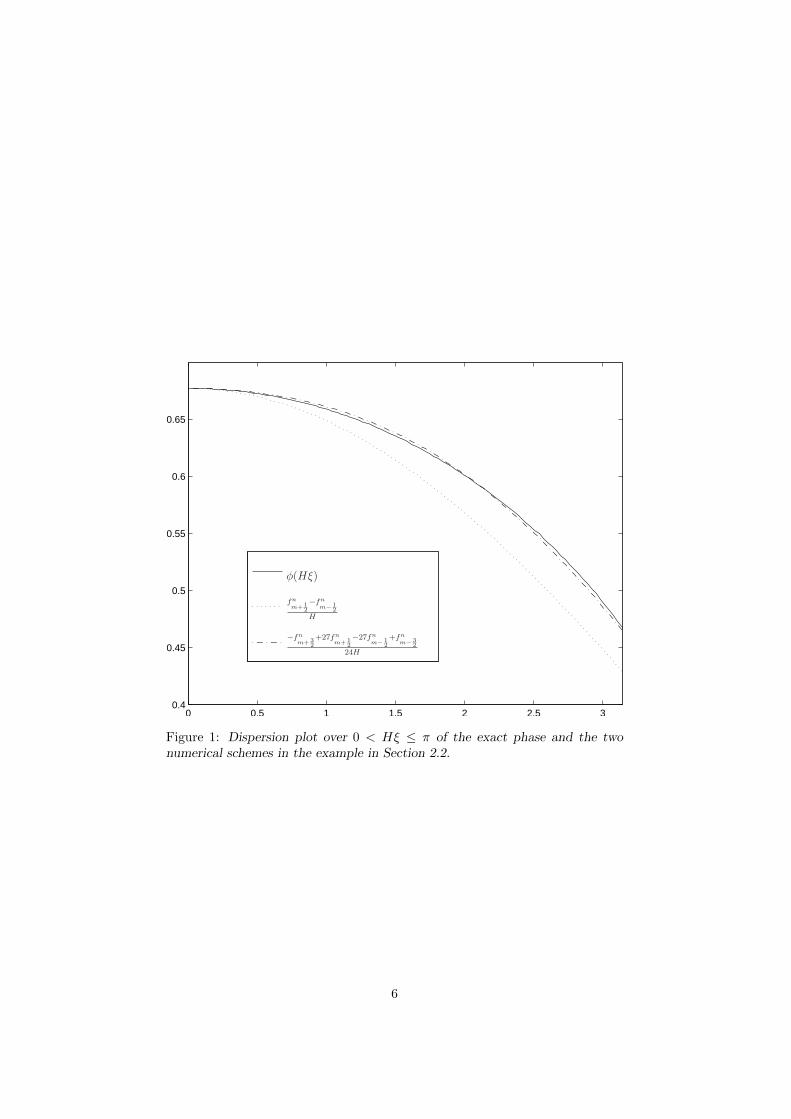
It is a fact that the schemes (4) and (5) are non-dissipative, see [13, 6],meaning that the amplification factor g satisfies that |g| = 1. The major sourceof concern is therefore the numerical phase error with respect to the exact phase.We will study the phase error for the two schemes above in relation to the exactphase, given below. The solution to (1) with f as in (2.2), is of the form,

u(x, t) =1√2π

∫ ∞−∞

u+(ω)eiω(x+t√A−βε2ω2) + u−(ω)eiω(x−t

√A−βε2ω2) dω,

where u+ and u− are given from the initial data, [13]. To simplify the analysiswe assume that the initial data is such that u+ = 0 and we have a right goingwave. The Fourier transform of u satisfies

u(ω, t+ ∆t) = e−i∆tω√A−βε2ω2

u(ω, t).

We define the phase speed φ for frequency ω as

φ(ω) =

√A− βε2ω2,

and the numerical phase speed α is defined by, [13]

g = |g|e−i∆tα(ω),

where g is the amplification factor of the numerical scheme.We show a dispersion plot for the exact phase and the two numerical phases

for the schemes (4) and (5) in Figure 1, where we have used the followingparameters:

ε = 0.01, Aε(x) = 1.1 + sin2πx

ε,

A =√

0.21, β = 0.01078280318,

H =1

150, K =

H

2.

2.3 Matrix formulation

We have chosen to use a matrix formulation for our finite difference solvers.Matlab is very efficient on sparse matrix times vector operations and it is sim-ple to produce discrete difference operators as sparse matrices. In Table 3 wedemonstrate the technique described below.

5

0 0.5 1 1.5 2 2.5 30.4

0.45

0.5

0.55

0.6

0.65

fn

m+12

−fn

m− 12

H

−fn

m+32

+27fn

m+12

−27fn

m− 12

+fn

m− 32

24H

φ(Hξ)

Figure 1: Dispersion plot over 0 < Hξ ≤ π of the exact phase and the twonumerical schemes in the example in Section 2.2.

6

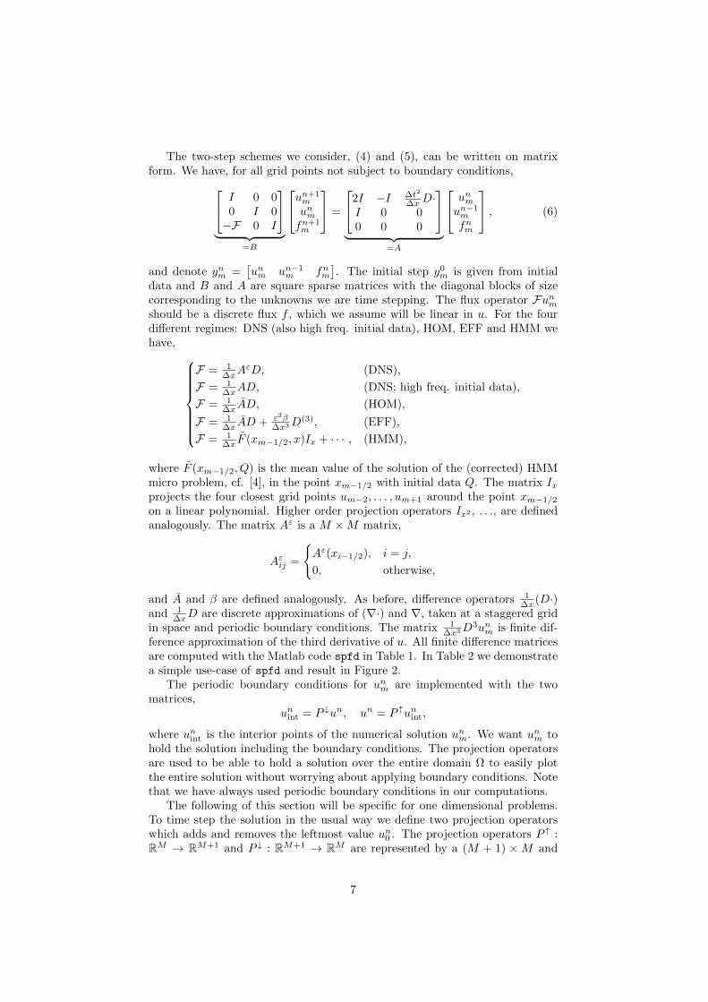
The two-step schemes we consider, (4) and (5), can be written on matrixform. We have, for all grid points not subject to boundary conditions, I 0 0

0 I 0−F 0 I

︸ ︷︷ ︸

=B

un+1m

unmfn+1m

=

2I −I ∆t2

∆xD·I 0 00 0 0

︸ ︷︷ ︸

=A

unmun−1m

fnm

, (6)

and denote ynm =[unm un−1

m fnm]. The initial step y0

m is given from initialdata and B and A are square sparse matrices with the diagonal blocks of sizecorresponding to the unknowns we are time stepping. The flux operator Funmshould be a discrete flux f , which we assume will be linear in u. For the fourdifferent regimes: DNS (also high freq. initial data), HOM, EFF and HMM wehave,

F = 1∆xA

εD, (DNS),

F = 1∆xAD, (DNS; high freq. initial data),

F = 1∆x AD, (HOM),

F = 1∆x AD + ε2β

∆x3D(3), (EFF),

F = 1∆x F (xm−1/2, x)Ix + · · · , (HMM),

where F (xm−1/2, Q) is the mean value of the solution of the (corrected) HMMmicro problem, cf. [4], in the point xm−1/2 with initial data Q. The matrix Ixprojects the four closest grid points um−2, . . . , um+1 around the point xm−1/2

on a linear polynomial. Higher order projection operators Ix2 , . . ., are definedanalogously. The matrix Aε is a M ×M matrix,

Aεij =

Aε(xi−1/2), i = j,

0, otherwise,

and A and β are defined analogously. As before, difference operators 1∆x (D·)

and 1∆xD are discrete approximations of (∇·) and ∇, taken at a staggered grid

in space and periodic boundary conditions. The matrix 1∆x3D

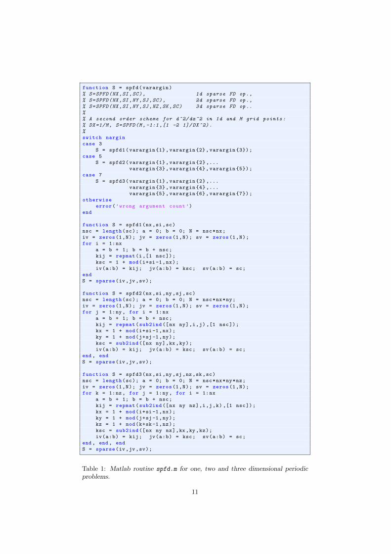
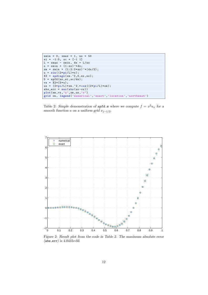
3unm is finite dif-ference approximation of the third derivative of u. All finite difference matricesare computed with the Matlab code spfd in Table 1. In Table 2 we demonstratea simple use-case of spfd and result in Figure 2.

The periodic boundary conditions for unm are implemented with the twomatrices,

unint = P ↓un, un = P ↑unint,

where unint is the interior points of the numerical solution unm. We want unm tohold the solution including the boundary conditions. The projection operatorsare used to be able to hold a solution over the entire domain Ω to easily plotthe entire solution without worrying about applying boundary conditions. Notethat we have always used periodic boundary conditions in our computations.

The following of this section will be specific for one dimensional problems.To time step the solution in the usual way we define two projection operatorswhich adds and removes the leftmost value un0 . The projection operators P ↑ :RM → RM+1 and P ↓ : RM+1 → RM are represented by a (M + 1) ×M and

7

M × (M + 1) matrix respectively,

P ↑ij =

1, i = 1 and j = M,

1, i > 1 and i− 1 = j,

0, otherwise,

P ↓ij =

0, j = 1,

1, i = j + 1,

0, otherwise.

We can more easily understand what P ↑ and P ↓ does on a pair of grid functions,

P ↑

u1

u2

...uM

=

uMu1

...uM

, P ↓

u0

u1

...uM

=

u1

u2

...uM

.

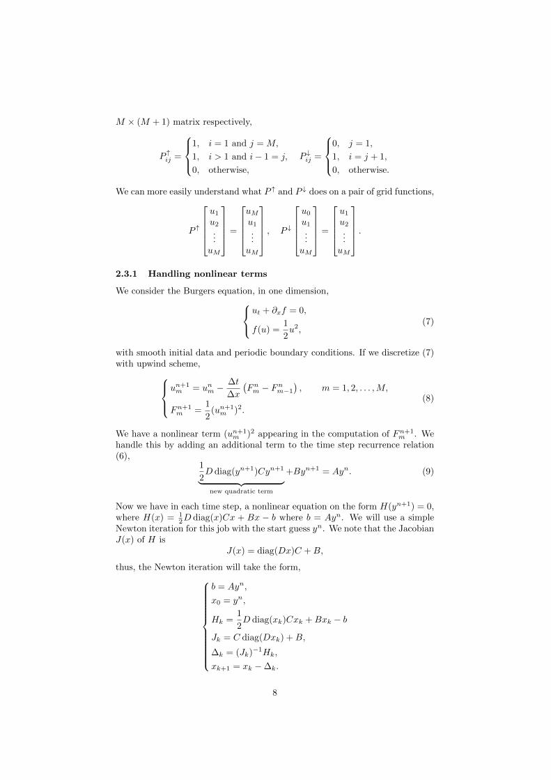
2.3.1 Handling nonlinear terms

We consider the Burgers equation, in one dimension,ut + ∂xf = 0,

f(u) =1

2u2,

(7)

with smooth initial data and periodic boundary conditions. If we discretize (7)with upwind scheme,

un+1m = unm −

∆t

∆x

(Fnm − Fnm−1

), m = 1, 2, . . . ,M,

Fn+1m =

1

2(un+1m )2.

(8)

We have a nonlinear term (un+1m )2 appearing in the computation of Fn+1

m . Wehandle this by adding an additional term to the time step recurrence relation(6),

1

2D diag(yn+1)Cyn+1︸ ︷︷ ︸

new quadratic term

+Byn+1 = Ayn. (9)

Now we have in each time step, a nonlinear equation on the form H(yn+1) = 0,where H(x) = 1

2D diag(x)Cx + Bx − b where b = Ayn. We will use a simpleNewton iteration for this job with the start guess yn. We note that the JacobianJ(x) of H is

J(x) = diag(Dx)C +B,

thus, the Newton iteration will take the form,

b = Ayn,

x0 = yn,

Hk =1

2D diag(xk)Cxk +Bxk − b

Jk = C diag(Dxk) +B,

∆k = (Jk)−1Hk,

xk+1 = xk −∆k.

8

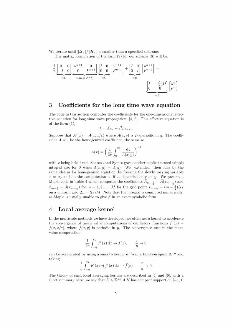
We iterate until ‖∆k‖/‖Hk‖ is smaller than a specified tolerance.The matrix formulation of the form (9) for our scheme (8) will be,

1

2

[0 0−I 0

]︸ ︷︷ ︸

=D

[un+1 0

0 Fn+1

]︸ ︷︷ ︸

=diag(yn+1)

[I 00 0

]︸ ︷︷ ︸

=C

[un+1

Fn+1

]+

[I 00 I

]︸ ︷︷ ︸

=B

[un+1

Fn+1

]=

[I −∆t

∆xD0 0

]︸ ︷︷ ︸

=A

[un

Fn

].

3 Coefficients for the long time wave equation

The code in this section computes the coefficients for the one-dimensional effec-tive equation for long time wave propagation, [4, 6]. This effective equation isof the form (1),

f = Aux + ε2βuxxx.

Suppose that Aε(x) = A(x, x/ε) where A(x, y) is 2π-periodic in y. The coeffi-cient A will be the homogenized coefficient, the same as,

A(x) =

(1

2π

∫ 2π

0

dy

A(x, y)

)−1

with x being held fixed. Santosa and Symes gave another explicit nested trippleintegral also for β when A(x, y) = A(y). We “extended” their idea by thesame idea as for homogenized equation, by freezing the slowly varying variablex = x0 and do the computation as if A depended only on y. We present aMaple code in Table 4 which computes the coefficients Am− 1

2= A(xm− 1

2) and

βm− 12

= β(xm− 12) for m = 1, 2, . . . ,M for the grid point xm− 1

2= (m − 1

2 )∆x

on a uniform grid ∆x = 2π/M . Note that the integral is computed numerically,as Maple is usually unable to give β in an exact symbolic form.

4 Local average kernel

In the multiscale methods we have developed, we often use a kernel to acceleratethe convergence of mean value computations of oscillatory functions fε(x) =f(x, x/ε), where f(x, y) is periodic in y. The convergence rate in the meanvalue computation,

1

2η

∫ η

−ηfε(x) dx→ f(x),

ε

η→ 0,

can be accelerated by using a smooth kernel K from a function space Kp,q andtaking

1

η

∫ η

−ηK (x/η) fε(x) dx→ f(x)

ε

η→ 0.

The theory of such local averaging kernels are described in [4] and [6], with ashort summary here: we say that K ∈ Kp,q if K has compact support on [−1, 1]

9

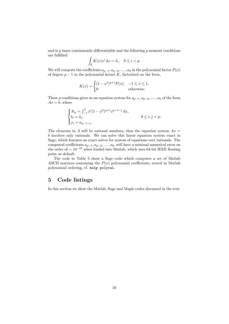
and is q times continuously differentiable and the following p moment conditionsare fulfilled: ∫

RK(x)xi dx = δi, 0 ≤ i < p.

We will compute the coefficients ap−1, ap−2, . . . , a0 in the polynomial factor P (x)of degree p− 1 in the polynomial kernel K, factorized on the form,

K(x) =

(1− x2)q+1P (x), −1 ≤ x ≤ 1,

0 otherwise.

These p conditions gives us an equation system for ap−1, ap−2, . . . , a0 of the formAx = b, where

Aij =∫ 1

−1xi(1− x2)q+1xp−1−j dx,

bi = δi,

xi = ap−1−i,

0 ≤ i, j < p.

The elements in A will be rational numbers, thus the equation system Ax =b involves only rationals. We can solve this linear equation system exact inSage, which features an exact solver for system of equations over rationals. Thecomputed coefficients ap−1, ap−2, . . . , a0, will have a minimal numerical error onthe order of ∼ 10−16 when loaded into Matlab, which uses 64-bit IEEE floatingpoint as default.

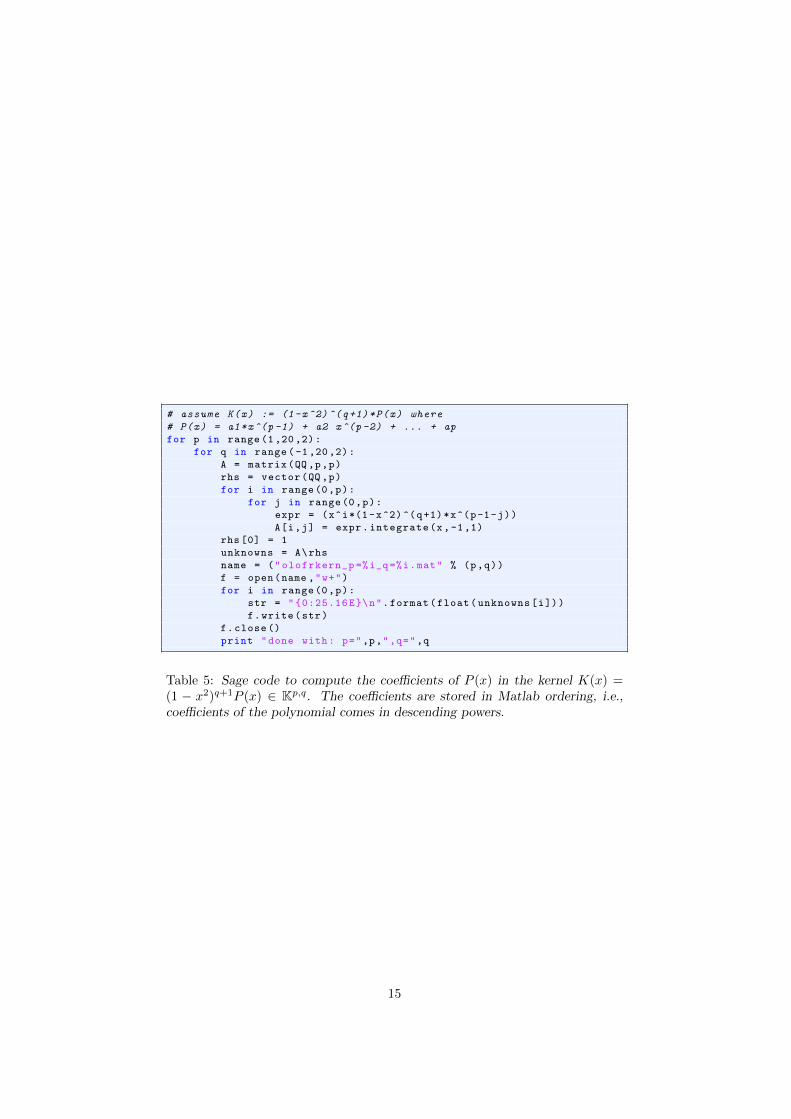
The code in Table 5 show a Sage code which computes a set of MatlabASCII matrices containing the P (x) polynomial coefficients, stored in Matlabpolynomial ordering, cf. help polyval.

5 Code listings

In this section we show the Matlab, Sage and Maple codes discussed in the text.

10

function S = spfd(varargin)

% S=SPFD(NX ,SI ,SC), 1d sparse FD op.,

% S=SPFD(NX ,SI ,NY ,SJ ,SC), 2d sparse FD op.,

% S=SPFD(NX ,SI ,NY ,SJ ,NZ ,SK ,SC) 3d sparse FD op..

%

% A second order scheme for d^2/ dx^2 in 1d and M grid points:

% DX =1/M, S=SPFD(M, -1:1 ,[1 -2 1]/ DX ^2).

%

switch nargin

case 3

S = spfd1(varargin 1, varargin 2, varargin 3);

case 5

S = spfd2(varargin 1, varargin 2 ,...

varargin 3, varargin 4, varargin 5);

case 7

S = spfd3(varargin 1, varargin 2 ,...

varargin 3, varargin 4 ,...

varargin 5, varargin 6, varargin 7);

otherwise

error(’wrong argument count ’)

end

function S = spfd1(nx,si ,sc)

nsc = length(sc); a = 0; b = 0; N = nsc*nx;

iv = zeros(1,N); jv = zeros(1,N); sv = zeros(1,N);

for i = 1:nx

a = b + 1; b = b + nsc;

kij = repmat(i,[1 nsc]);

ksc = 1 + mod(i+si -1,nx);

iv(a:b) = kij; jv(a:b) = ksc; sv(a:b) = sc;

end

S = sparse(iv,jv,sv);

function S = spfd2(nx,si ,ny,sj,sc)

nsc = length(sc); a = 0; b = 0; N = nsc*nx*ny;

iv = zeros(1,N); jv = zeros(1,N); sv = zeros(1,N);

for j = 1:ny, for i = 1:nx

a = b + 1; b = b + nsc;

kij = repmat(sub2ind ([nx ny],i,j) ,[1 nsc]);

kx = 1 + mod(i+si -1,nx);

ky = 1 + mod(j+sj -1,ny);

ksc = sub2ind ([nx ny],kx ,ky);

iv(a:b) = kij; jv(a:b) = ksc; sv(a:b) = sc;

end , end

S = sparse(iv,jv,sv);

function S = spfd3(nx,si ,ny,sj,nz ,sk,sc)

nsc = length(sc); a = 0; b = 0; N = nsc*nx*ny*nz;

iv = zeros(1,N); jv = zeros(1,N); sv = zeros(1,N);

for k = 1:nz, for j = 1:ny, for i = 1:nx

a = b + 1; b = b + nsc;

kij = repmat(sub2ind ([nx ny nz],i,j,k) ,[1 nsc]);

kx = 1 + mod(i+si -1,nx);

ky = 1 + mod(j+sj -1,ny);

kz = 1 + mod(k+sk -1,nz);

ksc = sub2ind ([nx ny nz],kx,ky,kz);

iv(a:b) = kij; jv(a:b) = ksc; sv(a:b) = sc;

end , end , end

S = sparse(iv,jv,sv);

Table 1: Matlab routine spfd.m for one, two and three dimensional periodicproblems.

11

xmin = 0, xmax = 1, nx = 50

si = -1:0, sc = [-1 1]

L = xmax - xmin , dx = L/nx

x = xmin + (1:nx)’*dx;

xm = xmin + (1:2:2* nx) ’*(dx/2);

u = sin ((2*pi/L)*x);

X2 = spdiags(xm.^2,0,nx ,nx);

D = spfd(nx,si ,sc/dx);

vx = X2*(D*u);

ux = (2*pi/L)*xm .^2.* cos ((2*pi/L)*xm);

abs_err = max(abs(ux-vx))

plot(xm ,vx,’x’,xm ,ux,’o’)

grid on, legend(’numerical ’,’exact ’,’location ’,’northwest ’)

Table 2: Simple demonstration of spfd.m where we compute f = x2ux for asmooth function u on a uniform grid xj−1/2.

0 0.1 0.2 0.3 0.4 0.5 0.6 0.7 0.8 0.9 1−2

−1

0

1

2

3

4

5

6

7

numericalexact

Figure 2: Result plot from the code in Table 2. The maximum absolute error(abs err) is 4.0431e-03.

12

eps =0.01 ,c=sqrt(sqrt (.21)),Tmax =1/c

M=1600 ,N=4000, axis_ =[0 1 -.1 1.1], plot_every_nth =10

dx=1/M,dt=Tmax/N,lambda=dt/dx,rho=eps/dx

A_func=@(x)1.1+ sin(2*pi*x/eps)

%A_func=@(x)repmat(c^2, size(x));

u0_func=@(x)exp ( -100*( mod(x,1) -0.5) .^2);

u1_func=@(x)zeros(size(x));

%ue_func=@(x,t)0.5*( u0_func(x+c*t)+u0_func(x-c*t));

x=(0:M) ’*dx;xi=x(2: end);xm =(1:2:2*M-1) ’*(dx/2);

I=speye(M,M);

Dm=spfd(M,[ 0 -1],[ 1 -1]);

Dp=spfd(M,[ 1 0],[ 1 -1]);

Aop=spdiags(A_func(xm),0,M,M);

Fop=Aop*Dm;

Pdown=[ sparse(M,1) speye(M,M)];

Pup=[ sparse(1,M-1) 1; speye(M,M)];

p=[1 M+1 2*M+1];q=[M 2*M 3*M];

pe=[1 M+2 2*M+2];qe=[M+1 2*M+2 3*M+1];

u=Pup*u0_func(xi);

f=1/dx*Fop*(Pdown*u);

uold=Pup*( u0_func(xi)-dt*u1_func(xi)+(dt ^2/(2* dx))*Dp*f);

y=[u;uold;f];

A=sparse (3*M,3*M);B=speye (3*M,3*M);

Ppre=blkdiag(Pdown ,Pdown ,I);

Ppost=blkdiag(Pup ,Pup ,I);

B(p(3):q(3),p(1):q(1))=-(1/dx)*Fop;

A(p(1):q(1),p(1):q(1))=2*I;

A(p(1):q(1),p(2):q(2))=-I;

A(p(1):q(1),p(3):q(3))=(dt^2/dx)*Dp;

A(p(2):q(2),p(1):q(1))=I;

for n=1:N

y=Ppost*(B\(A*(Ppre*y)));

if (mod(n,plot_every_nth)==0) ||(n==N)

plot(x,y(pe(1):qe(1)))

axis(axis_),drawnow

end

end

Table 3: An illustration of how we setup and use the matrix formulation inSection 2.3.

13

M := 100;

rho := y -> 1;

mu := y -> 11/10 + sin(y);

dx := 2*Pi/M:

avg := (f:: procedure) -> ( 1/(2* Pi)*integrate(f(x),x=0..2*Pi) ):

inv := (f:: procedure) -> ( x -> 1/f(x) ):

for m from 1 to M do

x0 := (m-1/2)*dx:

c2 := 1/(avg(rho)*avg(inv(mu))):

Omega1 := sqrt(c2):

p1 := Integrate(rho(y)*Integrate(inv(mu)(s)*

Integrate(rho(r),r=0..s),s=0..y),y=0..2*Pi):

p2 := Integrate(inv(mu)(y)*Integrate(rho(s)*

Integrate(inv(mu)(r),r=0..s),s=0..y),y=0..2*Pi):

p3 := Integrate(rho(y)*Integrate(inv(mu)(r),r=0..y),y=0..2*Pi):

d := 3* Omega1 ^3/(2* Pi^3) * p1

+ 3* Omega1 ^5* avg(rho)^2/(2* Pi^3) * p2

- 1/avg(inv(mu))*(1/ Omega1 + 3* Omega1/Pi^2 * p3

- 3* Omega1 ^3/(4* Pi^4) * p3^2):

Omega3 := Pi^2 * d / avg(rho):

alpha[m] := evalf [17]( Omega1 ^2);

beta[m] := evalf [10]( - Omega1*Omega3 /(3*2^2* Pi^2));

end do:

f := fopen("alpha_beta.mat", WRITE , TEXT):

for m from 1 to M do

fprintf(f,"%25.16E%25.16E%25.15E\n",

(m-1/2)*dx,alpha[m],beta[m]):

end do:

fclose(f):

Table 4: Maple code for computing the coefficients in the effective equation.The function ρ is an “undocumented feature”. Anything but ρ ≡ 1 should beconsidered untested. In our experiments we have always used ρ(x) = 1. Notethat the period of ρ and µ is assumed to be 2π-periodic in y, not 1.

14

# assume K(x) := (1-x^2) ^(q+1)*P(x) where

# P(x) = a1*x^(p -1) + a2 x^(p -2) + ... + ap

for p in range (1,20,2):

for q in range (-1,20,2):

A = matrix(QQ,p,p)

rhs = vector(QQ,p)

for i in range(0,p):

for j in range(0,p):

expr = (x^i*(1-x^2)^(q+1)*x^(p-1-j))

A[i,j] = expr.integrate(x,-1,1)

rhs [0] = 1

unknowns = A\rhs

name = ("olofrkern_p =%i_q=%i.mat" % (p,q))

f = open(name ,"w+")

for i in range(0,p):

str = "0:25.16E\n".format(float(unknowns[i]))

f.write(str)

f.close()

print "done with: p=",p,",q=",q

Table 5: Sage code to compute the coefficients of P (x) in the kernel K(x) =(1 − x2)q+1P (x) ∈ Kp,q. The coefficients are stored in Matlab ordering, i.e.,coefficients of the polynomial comes in descending powers.

15

6 Numerical schemes

Here we give a detailed description of the finite difference methods used for themacro and micro solvers used to solve wave propagation problems. The solversare designed for one, two and three dimensions in finite time. We also describea second order accurate scheme used for long time wave propagation problems.This scheme better captures the dispersive effects that are important in suchproblems. We have chosen to present the schemes in a HMM method contextwhere we have a macro solver with an unknown flux f (computed via microproblems) and micro solver with a known flux f = Aε∇u. The macro solverscan also be used as a solver when f is in fact known. In the case of finite timeproblems (HOM class) we have f = Au and for the effective equation for longtime (EFF class) we have f = Aux + βε2uxxx.

6.1 1D scheme

The finite difference scheme on the macro level has the formUn+1m = 2Unm − Un−1

m +K2Y nm,

Y nm =1

H

(Fnm+ 1

2− Fnm− 1

2

),

Fnm±1/2 = F (xm±1/2, Pnm±1/2),

where Pnm−1/2 = 1H

(Unm − Unm−1

). The micro level scheme defined analogously:

un+1m = 2unm − un−1

m + k2ynm,

ynm =1

h

(fnm+1/2 − f

nm−1/2

),

fnm−1/2 = am− 12

unm+1 − unmh

,

fnm+1/2 = am− 12

unm − unm−1

h.

6.2 2D scheme

A two dimensional problem is discretized with the following schemes: The finitedifference scheme on the macro level

Un+1m = 2Unm − Un−1

m +K2Y nm,

Y nm =1

H

(F

(1)

m+ 12 e1− F (1)

m− 12 e1

)+

1

H

(F

(2)

m+ 12 e2− F (2)

m− 12 e2

),

Fnm± 12 ek

= F (xm± 12 ek

, Pnm± 12 ek

),

(10)

where Pnm+ 1

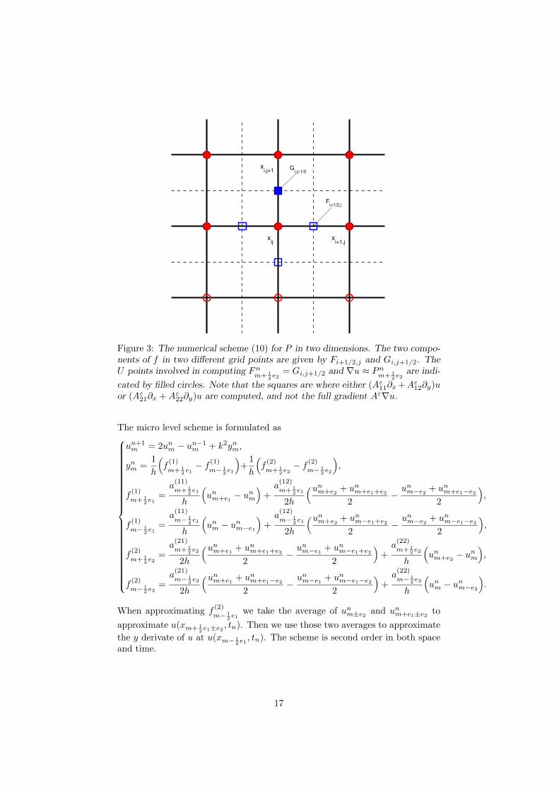
2 ekis given by (see Figure 3)

Pnm+ 12 e1

=[

1H (Um+e1 − Um) 1

2H

(Um+e2+Um+e2+e1

2 − Um−e2+Um−e2+e1

2

) ]T,

Pnm+ 12 e2

=[

12H

(Um+e1

+Um+e1+e2

2 − Um−e1+Um−e1+e2

2

)1H (Um+e2 − Um)

]T.

16

xij

xi+1,j

xi,j+1

Fi+1/2,j

Gi,j+1/2

Figure 3: The numerical scheme (10) for P in two dimensions. The two compo-nents of f in two different grid points are given by Fi+1/2,j and Gi,j+1/2. TheU points involved in computing Fn

m+ 12 e2

= Gi,j+1/2 and ∇u ≈ Pnm+ 1

2 e2are indi-

cated by filled circles. Note that the squares are where either (Aε11∂x +Aε12∂y)uor (Aε21∂x +Aε22∂y)u are computed, and not the full gradient Aε∇u.

The micro level scheme is formulated as

un+1m = 2unm − un−1

m + k2ynm,

ynm =1

h

(f

(1)

m+ 12 e1− f (1)

m− 12 e1

)+

1

h

(f

(2)

m+ 12 e2− f (2)

m− 12 e2

),

f(1)

m+ 12 e1

=a

(11)

m+ 12 e1

h

(unm+e1 − u

nm

)+a

(12)

m+ 12 e1

2h

(unm+e2 + unm+e1+e2

2−unm−e2 + unm+e1−e2

2

),

f(1)

m− 12 e1

=a

(11)

m− 12 e1

h

(unm − unm−e1

)+a

(12)

m− 12 e1

2h

(unm+e2 + unm−e1+e2

2−unm−e2 + unm−e1−e2

2

),

f(2)

m+ 12 e2

=a

(21)

m+ 12 e2

2h

(unm+e1 + unm+e1+e2

2−unm−e1 + unm−e1+e2

2

)+a

(22)

m+ 12 e2

h

(unm+e2 − u

nm

),

f(2)

m− 12 e2

=a

(21)

m− 12 e2

2h

(unm+e1 + unm+e1−e22

−unm−e1 + unm−e1−e2

2

)+a

(22)

m− 12 e2

h

(unm − unm−e2

).

When approximating f(2)

m− 12 e1

we take the average of unm±e2 and unm+e1±e2 to

approximate u(xm+ 12 e1±e2

, tn). Then we use those two averages to approximate

the y derivate of u at u(xm− 12 e1, tn). The scheme is second order in both space

and time.

17

6.3 3D scheme

The macro scheme for the three dimensional problem is on the formUnm = 2Unm − Un−1

m +K2Y nm,

Y nm =1

H

(F

(1,n)

m+ 12 e1− F (1,n)

m− 12 e1

)+

1

H

(F

(2,n)

m+ 12 e2− F (2,n)

m− 12 e2

)+

1

H

(F

(3,n)

m+ 12 e3− F (3,n)

m− 12 e3

),

Fnm± 12 ek

= F (xm± 12 ek

, Pnm± 12 ek

),

where Pnm+ 1

2 ekis defined as,

Pnm+ 12 e1

=

1H (Um+e1 − Um)

12H

(Um+e2

+Um+e2+e1

2 − Um−e2+Um−e2+e1

2

)1

2H

(Um+e3

+Um+e3+e1

2 − Um−e3+Um−e3+e1

2

) ,

Pnm+ 12 e2

=

1

2H

(Um+e1

+Um+e1+e2

2 − Um−e1+Um−e1+e2

2

)1H (Um+e2 − Um)

12H

(Um+e3+Um+e3+e2

2 − Um−e3+Um−e3+e2

2

) ,

Pnm+ 12 e3

=

1

2H

(Um+e1+Um+e1+e3

2 − Um−e1+Um−e1+e3

2

)1

2H

(Um+e2+Um+e2+e3

2 − Um−e2+Um−e2+e3

2

)1H (Um+e3 − Um)

.

18

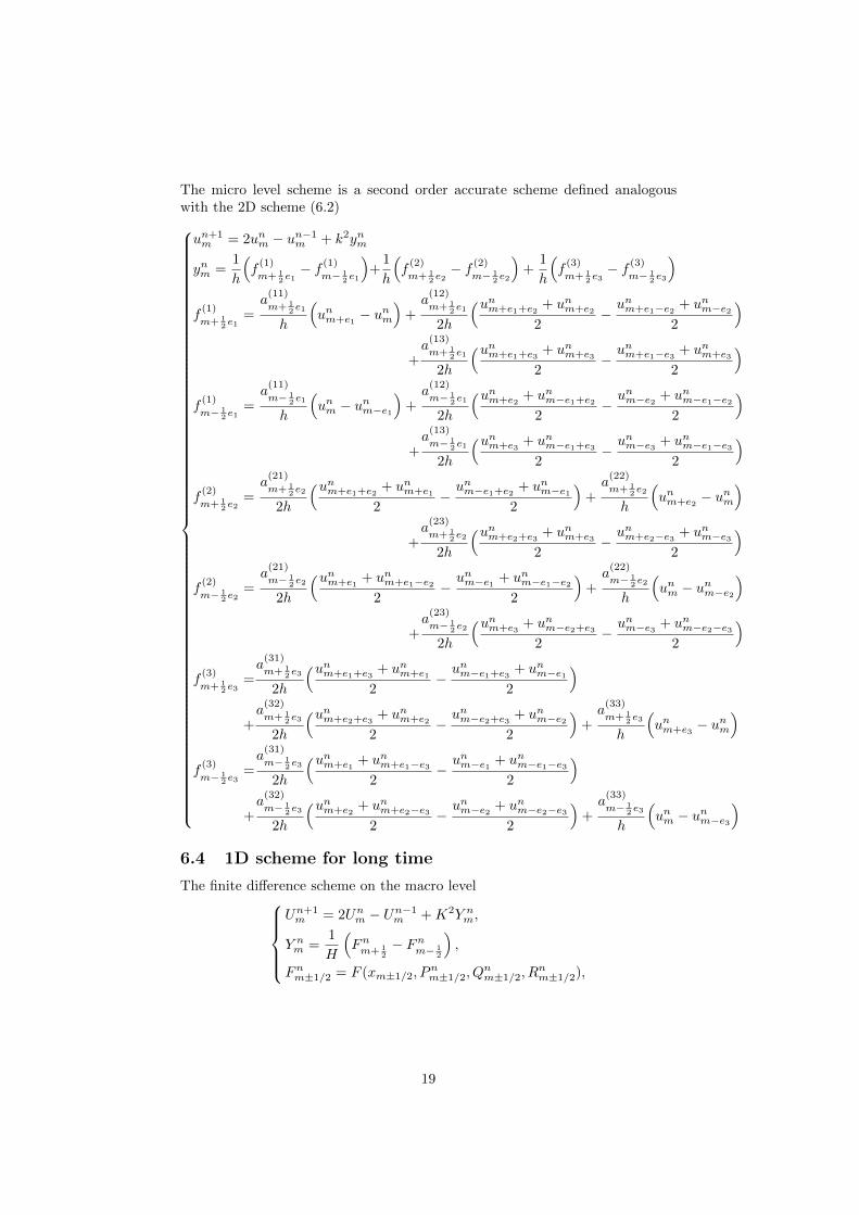
The micro level scheme is a second order accurate scheme defined analogouswith the 2D scheme (6.2)

un+1m = 2unm − un−1

m + k2ynm

ynm =1

h

(f

(1)

m+ 12 e1− f (1)

m− 12 e1

)+

1

h

(f

(2)

m+ 12 e2− f (2)

m− 12 e2

)+

1

h

(f

(3)

m+ 12 e3− f (3)

m− 12 e3

)f

(1)

m+ 12 e1

=a

(11)

m+ 12 e1

h

(unm+e1 − u

nm

)+a

(12)

m+ 12 e1

2h

(unm+e1+e2 + unm+e2

2−unm+e1−e2 + unm−e2

2

)+a

(13)

m+ 12 e1

2h

(unm+e1+e3 + unm+e3

2−unm+e1−e3 + unm+e3

2

)f

(1)

m− 12 e1

=a

(11)

m− 12 e1

h

(unm − unm−e1

)+a

(12)

m− 12 e1

2h

(unm+e2 + unm−e1+e2

2−unm−e2 + unm−e1−e2

2

)+a

(13)

m− 12 e1

2h

(unm+e3 + unm−e1+e3

2−unm−e3 + unm−e1−e3

2

)f

(2)

m+ 12 e2

=a

(21)

m+ 12 e2

2h

(unm+e1+e2 + unm+e1

2−unm−e1+e2 + unm−e1

2

)+a

(22)

m+ 12 e2

h

(unm+e2 − u

nm

)+a

(23)

m+ 12 e2

2h

(unm+e2+e3 + unm+e3

2−unm+e2−e3 + unm−e3

2

)f

(2)

m− 12 e2

=a

(21)

m− 12 e2

2h

(unm+e1 + unm+e1−e22

−unm−e1 + unm−e1−e2

2

)+a

(22)

m− 12 e2

h

(unm − unm−e2

)+a

(23)

m− 12 e2

2h

(unm+e3 + unm−e2+e3

2−unm−e3 + unm−e2−e3

2

)f

(3)

m+ 12 e3

=a

(31)

m+ 12 e3

2h

(unm+e1+e3 + unm+e1

2−unm−e1+e3 + unm−e1

2

)+a

(32)

m+ 12 e3

2h

(unm+e2+e3 + unm+e2

2−unm−e2+e3 + unm−e2

2

)+a

(33)

m+ 12 e3

h

(unm+e3 − u

nm

)f

(3)

m− 12 e3

=a

(31)

m− 12 e3

2h

(unm+e1 + unm+e1−e32

−unm−e1 + unm−e1−e3

2

)+a

(32)

m− 12 e3

2h

(unm+e2 + unm+e2−e32

−unm−e2 + unm−e2−e3

2

)+a

(33)

m− 12 e3

h

(unm − unm−e3

)6.4 1D scheme for long time

The finite difference scheme on the macro levelUn+1m = 2Unm − Un−1

m +K2Y nm,

Y nm =1

H

(Fnm+ 1

2− Fnm− 1

2

),

Fnm±1/2 = F (xm±1/2, Pnm±1/2, Q

nm±1/2, R

nm±1/2),

19

where P , Q and R are defined via U ,Pnm−1/2 =

−Um+1 + 27Um − 27Um−1 + Um−2

24H= Ux(xm−1/2, tn) +O(H4),

Qnm−1/2 =Um+1 − Um − Um−1 + Um−2

2H2= Uxx(xm−1/2, tn) +O(H2),

Rnm−1/2 =Um+1 − 3Um + 3Um−1 − Um−2

H3= Uxxx(xm−1/2, tn) +O(H2).

The micro level scheme has better dispersive properties than the normal twopoint divergence approximation, cf. Section 2.2,

un+1m = 2unm − un−1

m + k2ynm,

ynm =1

24h

(−fnm− 3

2+ 27fnm− 1

2− 27fnm+ 1

2+ fnm+ 3

2

),

fnm+ 32

=am+ 3

2

24h

(−unm+3 + 27um+2 − 27um+1 + um

),

fnm+ 12

=am+ 1

2

24h

(−unm+2 + 27um+1 − 27um + um−1

),

fnm− 12

=am− 1

2

24h

(−unm+1 + 27um − 27um−1 + um−2

),

fnm− 32

=am− 3

2

24h

(−unm + 27um−1 − 27um−2 + um−3

).

References

[1] Doina Cioranescu and Patrizia Donato. An Introduction to Homogeniza-tion. Number 17 in Oxford Lecture Series in Mathematics and its Appli-cations. Oxford University Press Inc., 1999.

[2] Bjorn Engquist, Henrik Holst, and Olof Runborg. Multiscale methods forthe wave equation. In Sixth International Congress on Industrial AppliedMathematics (ICIAM07) and GAMM Annual Meeting, volume 7. Wiley,2007.

[3] Bjorn Engquist, Henrik Holst, and Olof Runborg. Analysis of HMM forone dimensional wave propagation problems over long time, 2011.

[4] Bjorn Engquist, Henrik Holst, and Olof Runborg. Multiscale methods forone dimensional wave propagation with high frequency initial data. Tech-nical report, School of Computer Science and Communication, KTH, 2011.TRITA-NA 2011:7.

[5] Bjorn Engquist, Henrik Holst, and Olof Runborg. Multiscale methods forthe wave equation. Comm. Math. Sci., 9(1):33–56, Mar 2011.

[6] Bjorn Engquist, Henrik Holst, and Olof Runborg. Multiscale methodsfor wave propagation in heterogeneous media over long time. In BjornEngquist, Olof Runborg, and Richard Tsai, editors, Numerical Analysisand Multiscale Computations, volume 82 of Lect. Notes Comput. Sci. Eng.,pages 167–186. Springer Verlag, 2011.

20

[7] Agnes Lamacz. Dispersive effective models for waves in heterogeneous me-dia. Math. Models Methods Appl. Sci., 21:1871–1899, 2011.

[8] R.J. LeVeque. Numerical Methods for Conservation Laws. Lecture Notesin Mathematics. Birkhauser Verlag AG, 1994. ISBN 9783764327231.

[9] Maplesoft. Maple 12 User Manual, 2008.

[10] MATLAB. 7.12.0.635 (R2011a). The MathWorks Inc., Natick, Mas-sachusetts, 2011.

[11] Fadil Santosa and William W. Symes. A dispersive effective medium forwave propagation in periodic composites. SIAM J. Appl. Math., 51(4):984–1005, 1991. ISSN 0036-1399.

[12] W. A. Stein et al. Sage Mathematics Software (Version 4.2.1). The SageDevelopment Team, 2009. http://www.sagemath.org.

[13] John C. Strikwerda. Finite Difference Schemes and Partial DifferentialEquations (2nd ed.). SIAM, 2004. ISBN 0898715679.

21