Algorithmic Trading and Information ∗

Terrence HendershottHaas School of Business

University of California at Berkeley

Ryan RiordanDepartment of Economics and Business Engineering

Karlsruhe Institute of Technology

June 21, 2011

Abstract

We examine algorithmic trades (AT) and their role in the price discovery process in the 30DAX stocks on the Deutsche Boerse in January 2008. AT liquidity demand represents 52% ofvolume and AT supplies liquidity on 50% of volume. AT act strategically by monitoring themarket for liquidity and deviations of price from fundamental value. AT consume liquidity whenit is cheap and supply liquidity when it is expensive. AT contribute more to the efficient priceby placing more efficient quotes and AT demanding liquidity to move the prices towards theefficient price.

∗We thank Bruno Biais, Doug Foster, and seminar and conference participants at the University of Texas atAustin, University of Sydney 4th Annual Microstructure Conference, New York University Courant Institute ofMathematical Sciences 2nd Annual Algorithmic Trading Conference, 2009 Workshop on Information Systems andEconomics, 2009 German Finance Association, and IDEI-R Conference on Investment Banking and Financial Marketsfor helpful comments. Hendershott gratefully acknowledges support from the Net Institute, the Ewing MarionKauffman Foundation, and the Lester Center for Entrepreneurship and Innovation at the Haas School at UC Berkeley.Riordan gratefully acknowledges support from the Deutsche Forschungsgemeinschaft - graduate school of Informationand Market Engineering at the Karlsruhe Institute of Technology. Data was provided by the Deutsche Boerse andby the Securities Industry Research Centre of Asia-Pacific (SIRCA) on behalf of Reuters.

1

1 Introduction

Technology has revolutionized the way financial markets function and the way financial assets

are traded. Two significant interrelated technological changes are investors using computers to

automate their trading processes and markets reorganizing themselves so virtually all markets are

now electronic limit order books (Jain (2005)). The speed and quality of access to such markets

encourages the use of algorithmic trading (AT; AT denotes algorithmic traders as well), commonly

defined as the use of computer algorithms to automatically make trading decisions, submit orders,

and manage those orders after submission. Because the trading process is central to efficient risk

sharing and price efficiency it is important to understand how AT is used and its role in the price

formation process. We examine these issues for DAX stocks (the 30 largest market capitalization

stocks) traded on the Deutsche Boerse (DB) with data identifying whether or not each trade’s

buyer and seller generated their order with an algorithm. Directly identifying AT is not possible

in most markets, so relatively little is known.1

Algorithms are used to trade in both agency and proprietary contexts (Hasbrouck and Saar

(2011)). Institutional investors utilize AT to trade large quantities gradually over time, thereby

minimizing market impact and implementation costs. Liquidity demanders use algorithms to try to

identify when a security’s price deviates from the efficient price by quickly processing information

contained in order flow and price movements in that security and other securities across markets.

Liquidity suppliers must follow a similar strategy to avoid being picked off. Proprietary algorithms

are often referred to as high-frequency traders (HFT). Studying AT facilitates our overall under-

standing of the importance of technological advances in financial market performance. Examining

HFT and lower frequency traders separately, which is not possible with our data, can provide

insights into AT’s application to particular investment and trading strategies.

Most markets offer volume discounts to attract the most active traders. The development costs

of AT typically lead to it being adopted first by high-volume users who automatically qualify for the

quantity discounts. The German competition authority did not allow for generic volume discounts,

1Biais and Weill (2008) theoretically examine the relation between AT, market monitoring, and liquidity dynamics.Chaboud, Chiquoine, Hjalmarsson, and Vega (2009) study AT in the foreign exchange market. Hendershott, Jones,and Menkveld (2011) use a proxy for AT to examine AT’s effect on liquidity in the equity market.

2

rather requires that such discounts have a cost sensitive component. The DB successfully asserted

that algorithm generated trading is lower cost and highly sensitive to fee reductions and therefore,

could receive quantity discounts. In December of 2006, the DB introduced its fee rebate program

for automated traders.2 The DB provided data on AT orders in the DAX stocks for the first three

weeks of January 2008.

AT initiate 52% of trading volume via marketable orders. AT initiate smaller trades with AT

initiating 68% of volume for trades of less than 500 shares and 23% of volume for trades of greater

than 10,000 shares. AT initiate trades quickly when spreads are small and cluster their trades

together. AT are more sensitive to human trading activity than humans are to AT trading activity.

These are all consistent with AT closely monitoring the market for trading opportunities. If an

algorithmic trader is constantly monitoring the market, the trader can break up their order into

small pieces to disguise their intentions and quickly react to changes in market conditions. AT

could also be trying to exploit small deviations of price from fundamentals.

Moving beyond unconditional measures of AT activity we estimate probit models of AT using

market condition variables incorporating the state of the limit order book and past volatility and

trading volume. We find that AT are more likely to initiate trades when liquidity is high in terms

of narrow bid-ask spreads and higher depth. AT liquidity demanding trades are not related to

volatility in the prior 15 minutes, but AT initiated trading is negatively related to volume in the

prior 15 minutes.

Just as algorithms are used to monitor liquidity in the market, algorithms may also be used to

identify and capitalize on short-run price predictability. We use a standard vector auto-regression

framework (Hasbrouck (1991a) and Hasbrouck (1991b)) to examine the return-order flow dynamics

for both AT and human trades. AT liquidity demanding trades play a more significant role in

discovering the efficient price than human trades. AT initiated trades have a more than 20% larger

permanent price impact than human trades. In terms of the total contribution to price discovery—

decomposing the variance of the efficient price into its trade-correlated and non trade-correlated

components—AT liquidity demanding trades help impound 40% more information than human

2The DB modified the fee rebate program on November 2, 2009, to a volume discount program. This effectivelyends the AT specific fee rebate at the DB.

3

trades. The larger percentage difference between AT and humans for the variance decomposition

as compared to the impulse response functions implies that the innovations in AT order flow are

greater than the innovations in human order flow. This is consistent with AT being able to better

disguise their trading intentions.

We also examine when AT supply liquidity via non-marketable orders. The nature of our data

makes it possible to build an AT-only limit order book, but makes it difficult to perfectly identify

when AT supply liquidity in transactions (see Section 3 for details). Therefore, we focus our analysis

on quoted prices associated with AT and humans. While AT supply liquidity for exactly 50% of

trading volume, AT are at the best price (inside quote) more often than humans. This AT-human

difference is more pronounced when liquidity is lower, demonstrating that AT supply liquidity more

when liquidity is expensive.

The role of AT quotes in the price formation process is also examined. We calculate the

information shares (Hasbrouck (1995)) for AT and human quotes. AT quotes play a larger role in

the price formation process than their 50% of trading volume. The information shares decompose

the changes in the efficient price into components that occur first in AT quotes, human quotes,

and appear contemporaneously in AT and human quotes with the corresponding breakdown being

roughly 50%, 40%, and 10%, respectively. The ability of AT to update quotes quickly based on

changing market conditions could allow AT to better provide liquidity during challenging market

conditions.

The results on AT liquidity supply and demand suggest that AT monitor liquidity and informa-

tion in the market. AT consume liquidity when it is cheap and supply liquidity when it is expensive,

smoothing out liquidity over time. AT also contribute more to the efficient price by having more

efficient quotes and AT demanding liquidity so as to move the prices towards the efficient price.

Casual observers often blame the recent increase in market volatility on AT.3 AT demanding liq-

uidity during times when liquidity is low could result in AT exacerbating volatility, but we find no

evidence of this. AT could also exacerbate volatility by not supplying liquidity when the liquidity

dries up. However, we find the opposite.

3For example, see “Algorithmic trades produce snowball effects on volatility,” Financial Times, December 5, 2008.

4

Section 2 relates our work to existing literature. Section 3 describes the algorithmic trading on

the Deutsche Boerse. Section 4 describes our data. Section 5 analyzes when and how AT demands

liquidity. Section 6 examines how AT demand liquidity relates to discovering the efficient price.

Section 7 studies when AT supply liquidity and its relation to discovering the efficient price. Section

8 concludes.

2 Related Literature

Due to the difficulty in identifying AT, most existing research directly addressing AT has used data

from brokers who sell AT products to institutional clients. Engle, Russell, and Ferstenberg (2007)

use execution data from Morgan Stanley algorithms to study the tradeoffs between algorithm

aggressiveness and the mean and dispersion of execution cost. Domowitz and Yegerman (2005)

study execution costs of ITG buy-side clients, comparing results from different algorithm providers.

Several recent studies use comprehensive data on AT. Chaboud, Chiquoine, Hjalmarsson, and

Vega (2009) study the development of AT in the foreign exchange market on the electronic broking

system (EBS) in three currency pairs euro-dollar, dollar-yen, and euro-yen. They find little relation

between AT and volatility, as do we. In contrast to our results, Chaboud, Chiquoine, Hjalmarsson,

and Vega (2009) find that non-algorithmic order flow accounts for most of the variance in FX

returns. There are several possible explanations for this surprising result: (i) EBS’ origins as an

interdealer market where algorithms were closely monitored; (ii) humans in an interdealer market

being more sophisticated than humans in equity markets; or (iii) there is relatively little private

information in FX. Chaboud, Chiquoine, Hjalmarsson, and Vega (2009) find that AT seem to

follow correlated strategies, which is consistent with our results of AT clustering together in time.

Hendershott, Jones, and Menkveld (2011) use a proxy for AT, message traffic, which is the sum of

order submissions, order cancelations, and trades. Unfortunately, such a proxy makes it difficult

to closely examine when and how AT behave and their precise role in the price formation process.

Hendershott, Jones, and Menkveld (2011) are able to use an instrumental variable to show that

AT improves liquidity and makes quotes more informative. Our results on AT liquidity supply

and demand being more informed are the natural mechanism by which AT would lead to more

5

informationally efficient prices.

Any analysis of AT relates to models of liquidity supply and demand. Liquidity supply involves

posting firm commitments to trade. These standing orders provide free-trading options to other

traders. Using standard option pricing techniques, Copeland and Galai (1983) value the cost of the

option granted by liquidity suppliers. The arrival of public information can make existing orders

stale and can move the trading option into the money. Foucault, Roell, and Sandas (2003) study

the equilibrium level of effort that liquidity suppliers should expend in monitoring the market to

avoid this risk. AT enables this kind of monitoring and adjustment of limit orders in response to

public information,4 but AT can also be used by liquidity demanders to pick off liquidity suppliers

who are not fast enough in adjusting their limit orders with public information. The monitoring

of the state of liquidity in the market and taking it when cheap and making it when expensive is

consistent with AT playing an important role in the make/take liquidity cycle modeled by Foucault,

Kadan, and Kandel (2008).

Algorithms are also used by traders who are trying to passively accumulate or liquidate a large

position. Bertsimas and Lo (1998) find that the optimal dynamic execution strategies for such

traders involves optimally braking orders into pieces so as to minimize cost.5 While such execution

strategies pre-dated wide-spread adoption of AT (cf. Keim and Madhavan (1995)), brokers now

automate the process with AT products.

For each component of the larger transaction, a trader (or algorithm) must choose the type

and aggressiveness of the order. Cohen, Maier, Schwartz, and Whitcomb (1981) and Harris (1998)

focus on the simplest static choice: market order versus limit order. If a trader chooses a non-

marketable limit order, the aggressiveness of the order is determined by its limit price (Griffiths,

Smith, Turnbull, and White (2000) and Ranaldo (2004)). Lo and Zhang (2002) find that execution

times are very sensitive to the choice of limit price. If limit orders do not execute, traders can

cancel them and resubmit them with more aggressive prices. A short time between submission and

cancelation suggests the presence of AT, and in fact Hasbrouck and Saar (2009) find that a large

4Rosu (2009) implicitly incorporates AT by assuming limit orders can be constantly adjusted. See Parlour andSeppi (2008) for a general survey on limit order markets.

5Almgren and Chriss (2000) extend this by considering the risk that arises from breaking up orders and slowlyexecuting them.

6

number of limit orders are canceled within two seconds on the INET trading platform (which is

now Nasdaq’s trading mechanism).

A number of papers analyze the high-frequency trading subset of AT. Biais and Woolley (2011)

provide background and survey research on HFT and AT. Brogaard (2010) examines a number of

topics in HFT. Hendershott and Riordan (2011) study the role of overall, aggressive, and passive

HFT trading in the permanent and transitory parts of price discovery. Kirilenko, Kyle, Samadi,

and Tuzun (2011) analyze HFT in the E-mini S&P 500 futures market during the May 6, 2010

flash crash. Jovanovic and Menkveld (2011) model HFT as middlemen in limit order markets and

study their welfare effects. Menkveld (2011) shows how one HFT firm enabled a new market to

gain market share.

3 Deutsche Boerse’s Automated Trading Program

The Deutsche Boerse’s order-driven electronic limit order book system is called Xetra (see Hau

(2001) for details).6 Orders are matched using price-time-display priority. Quantities available at

the 10 best bid and ask prices as well as numbers of participants at each level are disseminated

continuously. See the Appendix for further details on Xetra.

During our sample period Xetra had a 97% market share of German equities trading. With

such a dominant position the competition authorities (Bundeskartellamt) required approval of all fee

changes prior to implementation. Fee changes must meet the following criteria: (i) all participants

are treated equally; (ii) changes must have a cost-related justification; and (iii) fee changes are

transparent and accessible to all participants. Criterion (i) and (iii) ensure a level playing field for

all members and is comparable to regulation in the rest of Europe and North America. The second

criteria is the most important for this paper. AT are viewed as satisfying the cost justification for

the change, so DB could offer lower trading fees for AT.

In December of 2007 the DB introduced its Automated Trading Program (ATP) to increase the

volume of automated trading on Xetra. To qualify for the ATP an electronic system must deter-

mine the price, quantity, and submission time for orders. In addition, the Deutsche Boerse ATP

6Iceberg orders are allowed as on the Paris Bourse (cf. Venkataraman (2001)).

7

agreement requires that: (i) the electronic system must generate buy and sell orders independently

using a specific program and data; (ii) the generated orders must be channeled directly into the

Xetra system; and (iii) the exchange fees or the fees charged by the ATP member to its clients

must be directly considered by the electronic system when determining the order parameters.

Before being admitted to the ATP, participants must submit an high-level overview of the

electronic trading strategies they plan to employ. The level of disclosure required here is intended

to be low enough to not require ATP participants to reveal important details of their trading

strategies. Following admission to the ATP, the orders generated by each participant are audited

monthly for plausibility. If the order patterns generated do not match those suggested by the

strategy plan submitted by a participant or are considered likely to have been generated manually,

the participant will be terminated from the ATP and may also be suspended from trading on

Xetra. Conversations with the DB revealed that a small portion of AT orders may not be included

in the data set. The suspicion on the part of the DB is due to the uncommonly high number of

orders (message traffic) to executions of certain participants which is typical of AT. However, these

participants make up less than 1% of trades in total and are, therefore, unlikely to affect our results.

The ATP agreement and the auditing process ensure that most, if not all, of the orders submitted by

an ATP participant are electronically generated and that most, if not all, electronically generated

orders are included in our data.

The DB only charges fees for executed trades and not for submitted orders. The rebate for ATP

participants can be significant. The rebates are designed to increase with the total trade volume

per month. Rebates are up to a maximum of 60% for euro monthly volume above 30 billion. The

first Euro volume rebate level begins at a 250 million Euro volume and is 7.5%. Table 1 provides

an overview of the rebate per volume level.

[Insert Table 1 Here]

For an ATP participant with 1.9 billion euros in eligible volume, the percentage rebate would

8

be (volumes are in millions of euros):

(250 ∗ 0% + 250 ∗ 7.5% + 500 ∗ 15.0% + 900 ∗ 22.5%)/1, 900 = 15.6% (1)

In the example above, an ATP participant would receive a rebate of 15.6%. This translates

into roughly 14,000 euros in trading cost savings on 91,200 in total, and an additional 5,323 euros

savings on 61,500 in total in clearing and settlement costs. This rebate (14,000 + 5,323) translates

into a 0.1 basis point saving on the 1.9 billion in turnover. For high-frequency trading firms, whose

turnover is much higher than the amount of capital invested, the savings are significant.

The fee rebate for ATP participants is the sole difference in how orders are treated. AT orders

are displayed equivalently in the publicly disseminated Xetra limit order book. The Xetra matching

engine does not distinguish between AT and human orders. Therefore, there are no drawbacks for

an AT firm to become an ATP participant. Thus, we expect all AT to take advantage of the

lower fees by becoming ATP participants. From this point on we equate ATP participants with

algorithmic traders and use AT for both. We will refer to non-ATP trades and orders as human or

human-generated.

4 Data and Descriptive Statistics

The DB provided data contain all AT orders submitted in DAX stocks, the leading German stock

market index composed of the 30 largest and most liquid stocks, between January 1st and January

18th, 2008, a total of 13 trading days. This is combined with Reuters DataScope Tick History

data provided by the Securities Industry Research Centre of Asia-Pacific (SIRCA). The SIRCA

data contains two separate databases, one for transactions and another for order book updates.

Firms’ market capitalization on December 31, 2007 is gathered from the Deutsche Boerse website

and cross-checked against data posted directly on each company’s website.

Table 2 describes the 30 stocks in the DAX index. Market capitalization is as of December

31st, 2007, in billions of Euros. The smallest firm (TUI AG) is large at 4.81 billion Euros but

is more than 20 times smaller than the largest stock in the sample, Siemens AG. The standard

9

deviation of daily returns is calculated for each stock during the sample period. All other variables

are calculated daily during the sample period for each stock (30 stocks for 13 trading days for a

total of 390 observations). Means and standard deviations along with the minimum and maximum

values are reported across the 390 stock-day observations.

[Insert Table 2 Here]

DAX stocks are quite liquid. The average trading volume is 250 million euros per day with

5,344 trades per day on average. The number of trades per day implies that our data set contains

roughly 2 million transactions (5,344*390). Quoted half-spreads are calculated when trades occur.

The average quoted half-spread of 2.98 basis points is comparable to large and liquid stocks in other

markets. The effective spread is the absolute value of the difference between the transaction price

and the mid quote price (the average of the bid and ask quotes). Average effective spreads are only

slightly larger than quoted spreads, evidence that market participant seldom submit marketable

orders for depth at greater than the best bid or ask.

We measure depth in two ways. The first is the standard measure of the depth at the inside

quote: the average depth in euros at the best bid price and the best ask price. As with spreads,

depth is measured at the time of transactions. More depth allows traders to execute larger trades

without impacting the price, which corresponds to higher liquidity. However, if the width of the

spread varies over time, then comparisons of depth at the inside do not clearly correspond to levels

of liquidity, e.g., 50,000 euros at an inside spread of 10 basis points need not represent more liquidity

than 5,000 euros at an inside spread of 5 basis points if in the latter case there is sufficient additional

depth between 5 and 10 basis points. To account for time variation in the spread we calculate a

second depth measure using the limit order book. For each stock we aggregate the depth at bid

and ask prices that have a distance of less than three times that stock’s average quoted half-spread

from the quote midpoint at the time of transaction. We refer to this measure of depth that does

not depend on the spread at the time of the transaction as depth3. A similar measure is used in

Foucault and Menkveld (2008) to capture depth away from the best prices.

10

5 AT Liquidity Demand

To measure AT liquidity demand we create an AT trade-initiation variable AT and human trade-

initiation variable Hum. The AT variable takes the value 1 when a trade is initiated by an AT,

and is 0 otherwise. The Hum variable takes the value 1 when a trade is initiated by a human

and 0 otherwise. Panel A of Table 3 reports the fraction of euro trading volume for AT trades

by trade size and overall.7 Overall AT initiates 52% of euro volume and more than 60% of all

trades. AT initiation declines as trade size increases. AT is greater than 68% and 57% in the two

smallest trade-size categories (0-499 shares and 500-999 shares) and decreases to 23% in the largest

trade-size category (10,000+ shares). AT’s decline with trade size is consistent with AT being used

to breakup large orders into smaller trades as suggested by Bertsimas and Lo (1998).

[Insert Table 3 Here]

To better understand the nature of AT and human liquidity demand we perform a series of

analyses similar to those found in Biais, Hillion, and Spatt (1995). We report the results of two

separate and related analyses in Table 4. The first column of Panel A of Table 4, labeled uncondi-

tional, provides what fraction of trades sequences, i.e., AT followed by AT, AT followed by human,

etc., we expect if AT and human trades are randomly ordered. The other columns in Panel A are

essentially a contingency table documenting the probability of observing a trade of a specific type

after observing a previous trade with a given type. All rows sum up to 100% and can be interpreted

as probability vectors.

[Insert Table 4 Here]

The first column and row of Panel A in Table 4 shows that if AT and human trades were

randomly ordered 37.03% of the transactions would be AT followed by AT while in the data this

occurs 40.73% of the time. The result show that AT trades are more likely to follow AT trades

7For simplicity and comparability we use the U.S. SEC Rule 605 trade-size categories based on the number ofshares traded.

11

than we would expect unconditionally and that AT trades are more likely to be repeated on the

same side of the market. The same is true for human trades. This suggests that human and AT

liquidity demanding trading strategies differ.

Panel B extends the analysis of AT and humans trade sequence to include trade-size categories.

As in Biais, Hillion, and Spatt (1995) we highlight in bold the three largest values in a column. The

results are similar to the diagonal results reported in Biais, Hillion, and Spatt (1995) and predicted

theoretically in Parlour (1998). The diagonal finding implies that trades of the same type—AT or

human trades in the same trade-size category—follow other similar trades. This leads to a diagonal

effect where the highest probabilities lie on the diagonal. The largest probability by far is for small

AT trades: the AT 1t−1AT

1t probability of 48.70% is much higher than the unconditional probability

of 31.62%. This suggests that: (i) AT repeatedly use small trades to hide their information; (ii)

AT limit their transitory price impact; or (iii) that different AT are following related strategies.

Panel B also shows that AT seem to be sensitive to human order flow but humans are relatively

insensitive to AT order flow.

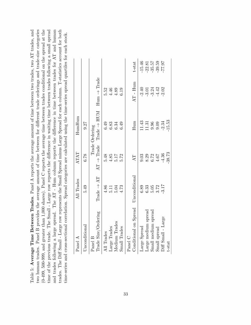
Table 4 provides evidence on the clustering of AT trades in trade sequences, but is not in-

formative on how closely together in time those trades cluster. Table 5 reports the average time

between trades dependent on past trades and spreads. As in Biais, Hillion, and Spatt (1995)

spreads are calculated for each stock and categories, e.g., large spread, are determined relative to

averages/percentiles for that stock. For example, large spread represents trades in a stock that

occur when spreads are in their widest quartile for that stock.

[Insert Table 5 Here]

The most interesting results in Table 5 are in Panel C. When spreads narrow the time until

the next AT trade shrinks significantly from 9.03 seconds for large spread to 4.67 seconds for small

spreads. While humans also respond more quickly to smaller spreads, the difference between large

spread (11.43 seconds) and small spreads (9.09 seconds) is 2.34 seconds for humans versus 4.36

seconds for AT. The difference-in-difference of 2.02 seconds between AT large-spread minus AT

small-spread and human large-spread minus human small-spread is statistically significant. This is

12

further evidence that AT actively monitor the market for liquidity.

Thus far we have studied AT and human sensitivity to past trades and spreads. Next we

inspect AT and human trading taking into account contemporaneous and lagged liquidity measures.

Following Barclay, Hendershott, and McCormick (2003) we use the liquidity variables summarized

in Table 2 and past return volatility and trading volume. Lagged volatility is the absolute value of

the stock return over the 15 minutes prior to the transaction. Lagged volume is the euro trading

volume in the 15 minutes prior to the transaction.

Table 6 reports coefficients estimates from probit regressions for AT initiated trades along with

their corresponding linear probability slopes and chi-square statistics. To control for stock effects

and time of day effects, we include, but do not report, firm dummy variables (30) and time of day

dummy variables (17 for each half-hour period). The only significant time of day effects are that

AT becomes less likely at the end of the trading day, primarily in the last half hour of continuous

trading. All 2, 085, 233 observations (each trade in our data set) are used. A chi-square statistic of

more than 3.84 represents statistical significant at the 5% level.

[Insert Table 6 Here]

The probit results generally show that AT is more likely to trade when spreads are narrow and

when trading volume over the prior 15 minutes is low. As in Panel A of Table 3 larger trades

are less likely to be initiated by AT. Volatility over the prior 15 minutes is unrelated to AT .

Once market conditions are controlled for, depth at the inside (depth) is unrelated to AT . Depth

measured independently of the inside spread (depth3) is positively related to AT . The positive

relation between AT initiation and liquidity and the zero relation between AT initiation and lagged

volatility provide no evidence to support the hypothesis that AT exacerbates volatility.

As with the spread results in the time until the next transaction analysis in Table 5, the depth

and spread results establish that AT are more likely to initiate trades when liquidity is high. AT

closely monitoring the book could bring about this result for two reasons. First AT could time their

liquidity demand for times when liquidity is cheap, as in the Foucault, Kadan, and Kandel (2008)

make/take liquidity cycle. When liquidity is expensive algorithms simply wait to trade when more

13

liquidity is available. A variant on this is that when liquidity is expensive AT attempt to capture

rather than pay the spread by switching from demanding liquidity to supplying liquidity, which we

explore in Section 7.

The results suggest that AT monitor the market for liquidity and consume liquidity when it

is cheap. This suggests that AT helps smooth out liquidity over time. When humans are more

willing to supply liquidity AT increase their liquidity demand. This together with AT having no

relationship to past volatility suggests that AT are more likely to dampen volatility than increase

volatility.

6 AT Liquidity Demand and Price Discovery

Having established that AT liquidity demand relates to liquidity dynamics we next examine the

dynamics between AT and returns. Just as AT monitors the market for variation in liquidity, AT

may be able to process and act on information before humans can. We examine this by estimating

the information content of AT and human trades using Hasbrouck (1991a) and Hasbrouck (1991b)

vector-autoregressions.

6.1 Information Content of AT - Impulse Response Function Results

To measure the information content of AT and human trades we first calculate the permanent price

impact of AT and human trades. Several papers have addressed related questions in multi-market

settings, e.g., for example, Huang (2002) and Barclay, Hendershott, and McCormick (2003) for

quoting and trading on electronic communications networks and Nasdaq. In settings with multiple

markets, variation in time stamps across markets make it difficult to ensure the proper ordering of

trades across different markets. In addition if time stamps are only reported in seconds, trades and

quote changes may occur contemporaneously. Our data avoid these potential issues because trading

is all within the DB Xetra system and time stamps are reported to the millisecond. Therefore, we

estimate the model on a trade-by-trade basis using 10 lags for AT and human trades. We estimate

the model for each stock for each day. We then conduct statistical inference using the 30 stocks *

13 days = 390 observations.

14

As in Barclay, Hendershott, and McCormick (2003) we estimate three equations, a midpoint

quote return equation, an AT equation, and a human trade equation. We use t, an event that is

a trade or quote change as our time scale and define qat as the signed (+1 for a buy, -1 for a sell)

AT trades and qhuman as the signed human trades. We define rt as the quote midpoint to quote

midpoint return between trades or quote changes. The VAR using 10 lags is as follows:

rt =10∑i=1

αirt−i +10∑i=0

βiqatt−i +

10∑i=0

γiqhumant−i + ε1,t, (2)

qatt =10∑i=1

δirt−i +10∑i=1

ρiqatt−i +

10∑i=1

ζiqhumant−i + ε2,t, (3)

qhumant =10∑i=1

πirt−i +10∑i=1

υiqatt−i +

10∑i=1

ψiqhumant−i + ε3,t, (4)

Each day the trading process restarts and all lagged values are set to zero. By estimating a

transaction by transaction VAR we ensure that there is no correlation between qatt and qhumant .

After estimating the VAR model, we follow Hasbrouck (1991a) and Hasbrouck (1991b) and invert

the VAR to get the vector moving average (VMA) model:

rt

qatt

qhumant

=

a(L) b(L) c(L)

d(L) e(L) f(L)

g(L) h(L) i(L)

ε1,t

ε2,t

ε3,t

,

where a(L) − i(L) are lagged polynomial operators. Following Hasbrouck (1991a), the impulse

response function for AT is∑10t=0 b(L) and can be interpreted as the private information content of

an innovation in AT. Similarly, the impulse response function for humans is∑10t=0 c(L). The impulse

response functions provide an estimate of the permanent price impact of a trade innovation (the

unexpected portion of a trade).

Table 7 reports the results of the impulse response function for 10 events into the future. We

also estimate the VAR out to 100 events and find no qualitatively different results. Table 7 reports

15

impulse response functions for each of the 30 stocks and the average impulse response function

across all 30 stocks. For each stock we estimate the statistical significance of the difference of the

impulse response function for AT and for human trading for the 13 trading days using Newey-West

standard errors. AT has a greater permanent price impact for 28 of the 30 stocks and for 23 of

those the AT-human difference is statistically significant at the 5% level. The average permanent

price impact for AT is 0.53 basis points versus 0.44 basis points for human trades. We estimate

the statistical significance of this 0.09 overall difference between AT and human trades by double

clustering standard errors on stock and trading day (Thompson (2006) and Petersen (2009)). In

summary, an innovation in AT trading leads to a more than 20% greater permanent price change

than an innovation in human trading.

[Insert Table 7 Here]

Figure 1 graphs the overall average (across stock days) of the cumulative impulse response

function of a positive (buy order) one standard deviation shock to AT and human order flow from

the immediate response to 10 events in the future. The initial impact of an AT trade innovation is

greater than for humans and the impact of AT versus humans trades increases over the subsequent

10 events. We also see that the impulse response functions are becoming flat by the tenth event.

Figure 1 shows that the price response to AT order flow is immediately greater than the response

to human order flow.

[Insert Figure 1 Here]

The 95% confidence intervals in Figure 1 show that the larger immediate impact of AT is

statistically significant. Following Chaboud, Chiquoine, Hjalmarsson, and Vega (2009) to analyze

whether the immediate reaction to AT is due to overreaction we report the difference between the

long-run (LR; 10 event forecast horizon) and short-run (SR; immediate) impulse response functions

in Table 8. As in Table 7 we report estimates for AT, humans, and the AT-human difference for

each stock and overall. The lagged adjustment (LR-SR) is smaller than the immediate response

16

to trading for both AT and human trades. The LR-SR impulse response is greater for AT than

humans in 24 stocks. 17 of the AT estimates are statistically significantly greater than humans

and in no stock is there statistically significant evidence that human trading has a larger impulse

response function than AT.

[Insert Table 8 Here]

The impulse response results provide evidence that individual innovations in AT have more

private information than human trades. This difference is persistent and increases beyond the

immediate impact of the trade. If AT contributed to transitory volatility the long-run impulse

response function should be lower than the short-run impulse response function. Our evidence is

more consistent with AT playing an important role in the efficient price formation process.

6.2 Aggregate Amount of Information in AT - Variance Decomposition

The impulse response functions reported above provide evidence that innovations in AT have a sig-

nificant impact on prices, but do not characterize how important the role of AT and human trading

are in the overall price formation process. To do this we follow Hasbrouck (1991b) to decompose

the variance of the efficient price into the portion of total price discovery that is correlated with AT

and human trades. Doing this first requires decomposing the midpoint return rt into its random

walk component mt and stationary component st:

rt = mt + st (5)

We refer to mt as the efficient price where mt = mt−1 + wt and Ewt = 0; st is the transitory

component. Using the previous VMA notation and defining σ2ε1 = Eε21,t, σ2ε2 = Eε22,t, and σ2ε3 =

Eε23,t, we decompose the variance of the efficient price into trade-correlated and trade-uncorrelated

changes:

σ2w =

(10∑i=0

ai

)2

σ2ε1 +

(10∑i=0

bi

)2

σ2ε2 +

(10∑i=0

ci

)2

σ2ε3 (6)

17

The second and third terms represent the proportion of the efficient price variance attributable

to AT and humans respectively. The first term is the public information (non-trade correlated)

portion of price discovery.8

Table 9 reports the variance decompositions results. As in the previous analyses, we report

the average by stock and overall. In 27 of the 30 stocks AT has a greater contribution to price

discovery and in 21 of those stocks the AT-human difference is statistically significant. In no stock

is the human contribution to price discovery statistically significantly greater than that of AT.

On average AT contributes 39% more to price discovery than do humans. The larger percentage

difference between AT and humans for the variance decomposition as compared to the impulse

response functions implies that the innovations in AT order flow are greater than the innovations

in human order flow. This is consistent with AT being able to disguise their trading intentions.

[Insert Table 9 Here]

We also calculate, but do not report for brevity, the short-run (immediate) variance decompo-

sition for AT and human trades. The results for the short-run variance decomposition are similar

to the results for the short-run impulse response functions in the previous section. Roughly half of

the variance explained by AT and human trades is reflected immediately.

7 AT Liquidity Supply and Price Discovery

Similar to the previous sections’ analysis of AT demanding liquidity and the role they plays in

the price discovery process, we would like to analyze how AT supply liquidity. By comparing the

volume of executed non-marketable AT orders with the total trading volume we can show that AT

supply liquidity on 50% of trading volume. Unfortunately, while our data from DB contains all

transactions where AT liquidity supply, we are only able to unambiguously identify 90% of these

8Because each trade is initiated either by AT or by humans the correlation in the trade equation residuals, ε2,tand ε3,t, is zero. Because the contemporaneous trade variables are included in the return equation the correlation ofthe residuals from the trade equations are uncorrelated with the residuals from the return equation. Therefore, wedo not include the residual covariance terms in the variance decomposition.

18

in the public transaction record.9 This is due to the frequency of trading, the time stamps from

the different data sources are not perfectly synchronized, and because knowing the size of a non-

marketable AT order does not uniquely identify the size of the total transaction. For example, if

a non-marketable AT order of 100 shares is executed the total trade size could be anything above

100 shares. Therefore, there are often several possible trades that occur at time stamps within

plausible differences between the public transaction record and our AT transaction record.10 This

limits the types of analysis we can perform.

While we are unable to exactly match AT liquidity supplying trades with trades in the SIRCA

public order book, we are able to build an AT order book and match this with the public order book.

To understand how AT supply liquidity we build two order books (see the Appendix for further

details). We build one AT order book that contains the best prices and sizes of AT orders and

compare this order book with the SIRCA full order book. The depth in the full SIRCA order book

that is not found in the AT order book is the human order book. We then keep the best/inside bid

and ask quotes for the AT and humans. If there is any doubt, each step in the matching procedure

assumes humans quote updates occur before AT quote updates.

We first examine whether or not AT are more likely to supply liquidity at the best quotes.

This provides initial evidence on whether or not AT are competitive in quoting the best prices for

marketable orders to trade with. Table 10 examines the amount of time AT and humans are at

the inside bid and ask. This combines the times when AT and humans are alone at the inside and

when they are both at the inside together. A positive number indicates that an AT is at the best

alone for longer than humans and the reverse is true if the value is negative.

[Insert Table 10 Here]

Table 10 shows that AT are at the inside more often in 24 of the 30 DAX stocks with the difference

9Analysis on the transactions that we can unambiguously identify as AT liquidity supplying supports the mainfindings in this section that AT supply liquidity when it is expensive and AT are less likely to trade against privateinformation.

10Multiple feasible matches for AT transactions also occur for liquidity demanding trades. However, when ATinitiates a trade size is uniquely identified, this only occurs on 0.1% of the AT liquidity demanding trades as opposedto 10% of the AT liquidity supplying trades.

19

being statistically significant in 21 of the stocks. On average for each stock-day AT are at the inside

almost 1 hour more per day than humans and the difference is statistically significant. Table 10

also examines whether or not AT are more likely to be present at the inside when spreads are wide

or narrow. As in Table 5 for each stock we identify times when spreads are wider and narrower

than average for that stock. We then calculate the amount of time, during the high- and low-spread

times, AT and humans are on the inside. Table 10 shows that AT are at the inside more often during

both high- and low-spread periods, but the AT-human difference is significantly higher during the

high-spread periods. This shows that AT are more likely to provide liquidity when it is expensive.

This is consistent with AT attempting to capture liquidity supply profits in the Foucault, Kadan,

and Kandel (2008) make/take liquidity cycle.

For AT to be on the inside more often yet only provide liquidity for for 50% of volume, AT orders

must be smaller or times when humans are alone at the inside are more likely to have transactions.

One natural explanation for trades occurring more often when humans are alone at the inside quote

is that the human quotes are stale and are adversely picked off. Examining how much the AT and

human quotes contribute to the price discover process will show if when AT and human quotes

are different the AT quotes better reflect the efficient price. If AT quotes contribute more to the

price discovery process then when human quotes differ from AT quotes the human quotes appear

inaccurate/stale.

7.1 Hasbrouck Information Shares

To examine AT and human quotes in the price discovery process we use the Information Shares (IS)

approach pioneered by Hasbrouck (1995). Typically this approach is used to determine which of

several markets contributes more to price discovery. This approach has been used in the literature

to compare spot and derivatives markets (e.g., Tse (1999) and Chan, Chung, and Fong (2002)) and

multiple stocks market (Hasbrouck (1995), Huang (2002), Barclay, Hendershott, and McCormick

(2003), and others). Because the information share has been widely used we briefly describe it. The

econometric approach assumes that AT and human quotes form a common efficient price process.

The information share attributable to AT and human quotes is the relative contribution of the

20

innovations of each to the innovation in the common efficient price. The general convention is to

equate the proportional information share to price discovery.

Because AT and human quotes are for the same stock arbitrage requires that the two price

series be co-integrated. We calculate the AT midpoint as MPATt = (BestBidATt + BestAskATt )/2

and the midpoint for humans is calculated in the same manner. The midpoints are assumed

covariance stationary. The information share of a participant is measured as that participants

contribution to the total variance of the common (random-walk) component. To formalize, denote

a price vector pt that represents the prevailing mid-quote for AT as pATt = mt + εATt and humans

as pHumt = mt + εHumt . mt, the common efficient price, is assumed to follow a random walk:

mt = mt−1 + ut, (7)

where E(ut) = 0, E(u2t) = σ2u, and E(utus) = 0 for t 6= s. The price vector can be represented

using a VMA model:

∆pt = εt + ψ1εt−1 + ψ2εt−2..., (8)

Where ε is a 2 X 1 vector of innovations with a zero mean and a variance matrix of Ω; εt =

[εATt , εHumt ] where εATt reflects the innovations (information) attributable to AT and εHumt to hu-

mans. The variance of the random walk component is then:

σ2u = ΨΩΨ′ (9)

where Ω = V ar(εt) and Ψ is a polynomial in the lag operator. Writing out the above equation

yields:

σ2u = [ΨAT ,ΨHum]

σ2at σat,hum

σhum,at σ2hum

ΨAT

ΨHum

.If the covariance matrix is diagonal the random-walk variance attributable to AT and humans can

be perfectly identified. If our record of the public limit order book was updated every time an order

arrived, there should be no contemporaneous correlation between AT and human quote changes.

21

However, it appears that at times the public order book dissemination contains multiple updates.

Therefore, the off-diagonal terms are not zero so we follow Hasbrouck (1995) to construct upper

and lower bounds for the information shares of AT and human quotes. The upper bound for AT

corresponds to the assumption that all of the contemporaneous correlation between AT and human

quote changes is attributable to AT; whereas the lower bound for AT assumes the contemporaneous

correlation between AT and human quote changes is attributable to humans.

Table 11 present the information share estimates using AT and human midpoint prices at 250

millisecond intervals. As with the impulse response and variance decompositions for AT liquidity

demand we calculate the information shares each day. We then conduct statistical significance based

on the 13 days for each stock. For the overall estimates we pool the 390 stock day information share

estimates and calculate standard errors controlling for correlation within each stock’s estimate and

controlling for correlation across stocks on the same day. It is worth recalling that our construction

of the AT and human quotes ensured that whenever there was uncertainty as to whether or not an

AT quote change preceded or followed a close by human quote change we assume the human quote

change occurred first. Therefore, the lower bound for the AT information share is truly a lower

bound, but the upper bound for AT information share is a lower bound for the true upper bound.

[Insert Table 11 Here]

Panel A reports the upper bound estimate for AT information shares and the lower bound for

human information shares. Panel B reverses the ordering to provide the lower bound estimate for

AT information shares and the upper bound for human information shares. The results in Panel

A of Table 11 show that in 18 of 30 stocks AT have statistically significantly higher information

shares. For the entire panel AT have an information share 21% higher with a t-statistic of 9.61. In

no stocks do humans have statistically significantly higher information shares than AT. We use the

same statistical framework as in the previous sections. In Panel B we see that the lower bound for

AT information shares is statistically significantly higher than the upper bound for humans in 11

stocks while the upper bound for humans is statistically significantly higher than the lower bound

for AT in 8 stocks. Overall, the lower bound on AT information shares is greater than the upper

22

bound for human, but the difference is not statistically significant.

Comparing the upper and lower bounds on AT and human information shares in Panels A and

B of Table 11 shows that 51% of price discovery comes from AT quotes, 39% of price discovery

comes from human quotes, and 10% occurs contemporaneously in AT and human quotes. Given

that we have ordered the quote changes to favor humans role in price discovery, we find evidence

to support AT playing a larger role in price discovery, but no evidence to suggest that humans play

a larger role.

8 Conclusion

We study algorithmic trading and its role in the price formation process. We find that AT consume

liquidity when it is cheap and provide liquidity when it is expensive. AT contributes more to the

discovery of the efficient price than human trading. These results demonstrate that AT closely

monitor the market in terms of liquidity and information and react quickly to changes in market

conditions. We find no evidence of AT behavior that would contribute to volatility beyond making

prices more efficient. The results are consistent with technology facilitating AT to more closely

resemble the Friedman (1953) stabilizing speculator. Further examinations of particular types of

AT, e.g., high-frequency trading, should provide insight into the potentially differing impact that

types of AT strategies may have.

Our results have important implications for academics, regulators, and market operators. The-

oretical models of limit order books should allow for a significant fraction of traders who closely

monitor the market. These traders could prevent prices from deviating significantly from funda-

mentals and prevent spreads from widening beyond a certain point; both of these features would

reduce the dimensionality of the state space (cf. Goettler, Parlour, and Rajan (2009)). The ATP

approved by the German competition authority appears to have led to behavior that should improve

both price efficiency and market liquidity in DAX stocks.

23

References

Almgren, R. and N. Chriss (2000). Optimal execution of portfolio transactions. Journal ofRisk 3 (2), 5–40.

Barclay, M., T. Hendershott, and D. McCormick (2003). Competition among trading venues: In-formation and trading on electronic communications networks. The Journal of Finance 58 (6),2637–2666.

Bertsimas, D. and A. Lo (1998). Optimal control of execution costs. Journal of Financial Mar-kets 1 (1), 1–50.

Bessembinder, H. (2003). Issues in assessing trade execution costs. Journal of Financial Mar-kets 6 (3), 233–257.

Biais, B., P. Hillion, and C. Spatt (1995). An empirical analysis of the limit order book and theorder flow in the paris bourse. Journal of Finance 50 (5), 1655–1690.

Biais, B. and P.-O. Weill (2008). Algorithmic trading and the dynamics of the order book.Manuscript, Toulouse University, IDEI.

Biais, B. and P. Woolley (2011). High frequency trading. Manuscript, Toulouse University, IDEI.

Brogaard, J. (2010). High frequency trading and its impact on market quality. Manuscript.

Chaboud, A., B. Chiquoine, E. Hjalmarsson, and C. Vega (2009). Rise of the machines: Algo-rithmic trading in the foreign exchange market. Technical report, FRB International FinanceDiscussion Paper No. 980.

Chan, K., Y. Chung, and W. Fong (2002). The informational role of stock and option volume.Review of Financial Studies 15 (4), 1049–1075.

Cohen, K., S. Maier, R. Schwartz, and D. Whitcomb (1981). Transaction costs, order placementstrategy and existence of the bid-ask spread. Journal of Political Economy 89 (2), 287–305.

Copeland, T. and D. Galai (1983). Information effects on the bid-ask spread. Journal of Fi-nance 38 (5), 1457–1469.

Domowitz, I. and H. Yegerman (2005). The cost of algorithmic trading: A first look at com-parative performance. Edited by Brian R. Bruce, Algorithmic Trading: Precision, Control,Execution. Institutional Investor .

Engle, R., J. Russell, and R. Ferstenberg (2007). Measuring and modeling execution cost andrisk. Manuscript, NYU Stern.

Foucault, T., O. Kadan, and E. Kandel (2008). Liquidity cycles and make/take fees in electronicmarkets. Manuscript, Toulouse University, IDEI.

Foucault, T. and A. Menkveld (2008). Competition for order flow and smart order routing sys-tems. Journal of Finance 63 (1), 119–158.

Foucault, T., A. Roell, and P. Sandas (2003). Market making with costly monitoring: An analysisof the soes controversy. Review of Financial Studies 16 (2), 345–384.

Friedman, M. (1953). The case for flexible exchange rates. In M. Friedman (Ed.), Essays inPositive Economics. Chicago: University of Chicago Press.

24

Goettler, R., C. Parlour, and U. Rajan (2009). Informed traders and limit order markets. Journalof Financial Economics 93 (1), 67–87.

Griffiths, M., B. Smith, D. Turnbull, and R. White (2000). The costs and determinants of orderaggressiveness. Journal of Financial Economics 56 (1), 65–88.

Harris, L. (1998). Optimal dynamic order submission strategies in some stylized trading problems.Financial Markets, Institutions, and Instruments 7 (2), 1–76.

Hasbrouck, J. (1991a). Measuring the information content of stock trades. Journal of Fi-nance 46 (1), 179–207.

Hasbrouck, J. (1991b). The summary informativeness of stock trades: An econometric analysis.Review of Financial Studies 4 (3), 571–595.

Hasbrouck, J. (1995). One security, many markets: Determining the contributions to price dis-covery. Journal of Finance 50 (4), 1175–1199.

Hasbrouck, J. and G. Saar (2009). Technology and liquidity provision: The blurring of traditionaldefinitions. Journal of Financial Markets 12 (2), 143–172.

Hasbrouck, J. and G. Saar (2011). Low latency trading. Manuscript.

Hau, H. (2001). Location matters: An examination of trading profits. The Journal of Fi-nance 56 (5), 1959–1983.

Hendershott, T., C. M. Jones, and A. J. Menkveld (2011). Does algorithmic trading improveliquidity? Journal of Finance 66 (1), 1–33.

Hendershott, T. and R. Riordan (2011). High frequency trading and price discovery. Manuscript.

Huang, R. (2002). The quality of ecn and nasdaq market maker quotes. Journal of Finance 57 (3),1285–1319.

Jain, P. (2005). Financial market design and the equity premium: Electronic versus floor trading.Journal of Finance 60 (6), 2955–2985.

Jovanovic, B. and A. Menkveld (2011). Middlemen in limit-order markets. Manuscript.

Keim, D. and A. Madhavan (1995). Anatomy of the trading process: Empirical evidence on thebehavior of institutional traders. Journal of Financial Economics 37 (3), 371–398.

Kirilenko, A., A. S. Kyle, M. Samadi, and T. Tuzun (2011). The flash crash: The impact of highfrequency trading on an electronic market. Manuscript.

Lee, C. and M. Ready (1991). Inferring trade direction from intraday data. Journal of Fi-nance 46 (2), 733–746.

Lo, A., M. A. and J. Zhang (2002). Econometric models of limit-order executions. Journal ofFinancial Economics 65 (1), 31–71.

Menkveld, A. (2011). High frequency trading and the new-market makers. Manuscript.

Parlour, C. (1998). Price dynamics in limit order markets. Review of Financial Studies 11 (4),789–816.

Parlour, C. and D. Seppi (2008). Limit order markets: A survey. Handbook of Financial Inter-mediation and Banking, edited by A.W.A. Boot and A.V. Thakor..

25

Petersen, M. (2009). Estimating standard errors in finance panel data sets: Comparing ap-proaches. Review of Financial Studies 22 (1), 435.

Ranaldo, A. (2004). Order aggressiveness in limit order book markets. Journal of FinancialMarkets 7 (1), 53–74.

Rosu, I. (2009). A dynamic model of the limit order book. Review of Financial Studies 22 (11).

Thompson, S. (2006). Simple formulas for standard errors that cluster by both firm and time.Mimeo, Harvard University.

Tse, Y. (1999). Price discovery and volatility spillovers in the djia index and futures markets.Journal of Futures Markets 19 (8), 911–930.

Venkataraman, K. (2001). Automated versus floor trading: An analysis of execution costs on theparis and new york exchanges. The Journal of Finance 56 (4), 1445–1485.

26

A Appendix - Xetra and AT Matching Details

The Xetra trading system is the electronic trading system operated by the Deutsche Boerse andhandles more than 98% of German equities trading by euro volume in DAX stocks (2007 DeutscheBoerse Factbook). The DB is a publicly traded company that also operates the Eurex deriva-tives trading platform and the Clearstream European clearing and settlement system. DB admitsparticipants that want to trade on Xetra based on regulations set and monitored by German andEuropean financial regulators. After being admitted participants can only connect electronically toXetra, floor trading is operated separately with no interaction between the two trading segments.

Xetra is implemented as an electronic limit order book with trading split into phases as fol-lows:

• Opening call auction with a random ending that opens trading at 9:00

• A continuous trading period

• A two-minute intra-day call auction at 1:00 with a random ending

• A second continuous trading period

• A closing call auction beginning at 5:30 with a random ending after 5:35

We focus our analysis on trade occurring during the two continuous trading periods. Liquidity inDAX stocks is provided by public limit orders displayed in the order book of each stock. Ordersexecute automatically when an incoming market, or marketable limit order crosses with an out-standing limit order. Order execution preference is determined using price-time priorities. Threetypes of orders are permitted, limit, market and iceberg orders. Iceberg orders are orders thatdisplay only a portion of the total size of an order. Iceberg orders sacrifice time priority on thenon-displayed portion. Pre-trade transparency includes the 10 best bids and ask prices and quan-tities but not the ID of the submitting participant (as on the Paris Bourse (Venkataraman (2001)).Trade price and size are disseminated immediately to all participants. The tick size for most stocksis 1 euro cent with the exception of two stocks that trade in tenths of a cent.11

A.1 Trade Matching

For trades we match two separate types of data. AT trades are matched with trades in the SIRCApublic data record. We also match the best (highest bid and lowest ask) AT orders with the SIRCApublic order book. Using the AT order data we identify AT liquidity demanding trades in the publicdata. We match these AT trades to the SIRCA data using the following criteria:

• Symbol

• Price

• Size

• Trade Direction

• Time stamp (milliseconds)

Matches between the data sources identify liquidity demanding trades (AT). Liquidity demand-ing trades match exactly with trade size and price in the public data. We identify the trade initiator

11Both stocks, Deutsche Telekom AG and Infineon AG have trade prices below 15 euros. Our sample periodoverlaps a Deutsche Boerse tick-size test that was subsequently extended to other stocks

27

in the SIRCA public data using the Lee and Ready trade direction algorithm Lee and Ready (1991)with the Bessembinder (2003) modifications to determine the trade direction in the public data anduse the modification and execution time stamp in the AT data.

Adjustments are made for an additional lag in the time stamp between the AT and SIRCA datasets. The publicly available data is time-stamped to the millisecond but, due to transmission andadditional system processing, it lags the system order data. We allow for a time window of up to250 ms in the public data when looking for a match of the remaining criteria. The below table A-1summarizes the lags needed to match trades by type.

Table A-1: Trade Matching by Type and Lag. This table reports distributions of lags betweenthe time stamps in the Deutsche Boerse System Order data and SIRCA public data used formatching.

Lag (MS) AT % of Total

000-050 324600 25.62%051-100 390456 30.82%101-150 270765 21.37%151-200 130655 10.31%201-250 76999 6.08%251-300 58765 4.64%301-500 14561 1.15%Total 1266801 100.00%

A.2 Quote Matching

We also match the quotes from non-marketable orders submitted by algorithms and humans. Todo so we create two order books. For the AT we re-create an AT order book based on the systemorder data. To create a human order book we take the SIRCA publicly disseminated order bookand ’subtract’ the AT order book. The SIRCA order book is disseminated with a lag, in this case,of not more than 250 ms. The 250 ms maximum lag was discovered by manual inspection of a largenumber of AT orders and SIRCA order books, especially around periods of high activity. Afterthe AT order book is created we match the best AT price and quantity with the next order bookupdate after the 250 ms lag. If there were no updates within 500 ms, we take the last updatebefore 250 ms. If we find a match and the AT price is ’better’ than the posted price we delete theAT record. This phenomena is likely related to fleeting orders described in Hasbrouck and Saar(2009). If an AT submits an order that only lives for a small of number of MS and is thereforefleeting, we will be unlikely to find it in the SIRCA public order data. Another case is when an ATsubmit a non-marketable limit order which is hit by an incoming marketable limit order directlyafter submission but before the 250 ms mark. This only occurs when AT orders live less than 250ms and the true lag is also less than 250 ms. If the quantity match isn’t exact we adjust the ATquantity to the lowest possible AT quantity. By performing these corrections we are essentiallyhandicapping AT and giving the benefit of the doubt to humans in general.

28

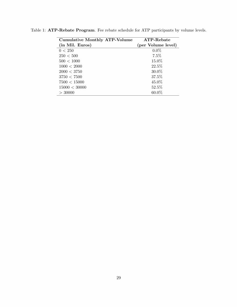
Table 1: ATP-Rebate Program. Fee rebate schedule for ATP participants by volume levels.

Cumulative Monthly ATP-Volume ATP-Rebate(in Mil. Euros) (per Volume level)

0 < 250 0.0%250 < 500 7.5%500 < 1000 15.0%1000 < 2000 22.5%2000 < 3750 30.0%3750 < 7500 37.5%7500 < 15000 45.0%15000 < 30000 52.5%> 30000 60.0%

29

Table 2: Summary Statistics. This table presents descriptive statistics for the 30 constituents ofthe DAX index between January 1, 2008 and January 18, 2008. The data set combines DeutscheBoerse Automated Trading Program System Order data and SIRCA trade, quote, and order data.Market Capitalization data is gathered from the Deutsche Boerse website and cross-checked againstdata posted directly on the company’s website and is the closing market capitalization on December31, 2007. Other variables are averaged per stock and day (390 observations) and the mean, std.dev., maximum and minimum of these stock-day averages are reported.

Variable Mean Std. Dev. Min Max

Mkt. Cap. (Euro Billion) 32.85 26.03 4.81 99.45Price (Euros) 67.85 42.28 6.45 155.15Std. Dev of Daily Return (%) 3.12 1.40 1.47 9.29Daily Trading Volume (Euro Million) 250 217 23 1,509Daily Number of Trades per Day 5,344 3,003 1,292 19,252Trade Size (Euro) 40,893 15,808 14,944 121,710Quoted Spread (bps) 2.98 3.01 1.24 9.86Effective Spread (bps) 3.49 3.05 1.33 10.05Depth (Euro 10 Million) 0.0177 0.0207 0.0044 0.1522Depth3 (Euro 10 Million) 0.1012 0.1545 0.0198 1.0689

30

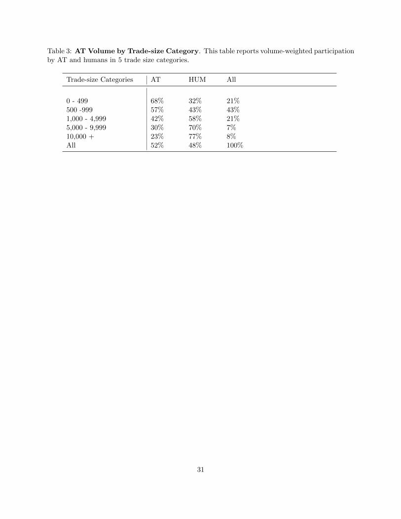
Table 3: AT Volume by Trade-size Category. This table reports volume-weighted participationby AT and humans in 5 trade size categories.

Trade-size Categories AT HUM All

0 - 499 68% 32% 21%500 -999 57% 43% 43%1,000 - 4,999 42% 58% 21%5,000 - 9,999 30% 70% 7%10,000 + 23% 77% 8%All 52% 48% 100%

31

Tab

le4:

Tra

deFre

quencyConditionalon

Pre

viousTra

de.

Pan

elA

rep

orts

the

con

dit

ion

alfr

equ

ency

of

ob

serv

ing

AT

an

dhu

man

trad

esaf

ter

obse

rvin

gtr

ades

ofot

her

par

tici

pan

ts.

Inco

lum

nan

dro

wh

ead

ingst

ind

exes

trad

es.AT

rep

rese

nts

AT

trad

esan

dHum

rep

rese

nts

hu

man

trad

es.

Pan

elB

pro

vid

esco

ndit

ion

alp

rob

abil

itie

sb

ased

onth

ep

revio

us

trad

e’s

size

an

dp

art

icip

ant

wit

hth

eth

ree

hig

hes

tva

lues

per

colu

mn

hig

hli

ghte

din

bol

d.

Pan

elA

Buy t−1

Sell t−1

Ord

erin

gU

nco

nd

.F

req.

Bu

yS

ell

Sell t

Buy t

ATt−

1ATt

37.0

3%40

.73%

13.7

3%10

.96%

7.84

%8.

20%

ATt−

1HUMt

23.8

2%20

.12%

5.53

%5.

05%

5.44

%4.

11%

HUMt−

1ATt

23.8

2%20

.12%

6.45

%5.

64%

3.89

%4.

15%

HUMt−

1HUMt

15.3

3%19

.02%

5.48

%5.

35%

3.75

%4.

45%

100.

00%

31.1

8%27

.00%

20.9

1%20

.91%

Pan

elB

AT5 t

AT4 t

AT3 t

AT2 t

AT1 t

Hum

5 tHum

4 tHum

3 tHum

2 tHum

1 t

AT5 t−

18.38%

9.46%

18.13%

16.7

8%7.

81%

8.16%

6.03%

6.74

%7.9

6%

10.5

4%

AT4 t−

13.82%

7.87%

15.97%

23.3

3%11

.71%

4.51%

4.61

%7.

36%

9.9

0%

10.9

4%

AT3 t−

11.

35%

2.73

%12

.00%

28.95%

20.6

9%2.

22%

2.70

%6.

23%

11.1

1%

12.0

3%

AT2 t−

10.

22%

0.70

%4.

69%

27.10%

33.88%

0.60

%1.

12%

4.07

%11.8

9%

15.7

2%

AT1 t−

10.

05%

0.18

%1.

75%

16.6

7%48.70%

0.17

%0.

45%

2.19

%9.8

9%

19.9

4%

Hum

5 t−1

5.46%

6.51%

13.72%

17.5

0%8.

30%

10.26%

7.15%

8.66%

10.3

5%

12.0

9%

Hum

4 t−1

1.80

%3.

36%

10.4

0%22

.56%

14.4

2%4.

24%

6.40%

9.77%

13.4

6%

13.5

8%

Hum

3 t−1

0.56

%1.

39%

6.78

%23.53%

21.1

7%1.

70%

2.75

%10.16%

16.36%

15.60%

Hum

2 t−1

0.20

%0.

54%

3.43

%19

.21%

28.3

7%0.

69%

1.31

%4.

95%

19.83%

21.47%

Hum

1 t−1

0.15

%0.

34%

2.20

%14

.98%

33.10%

0.56

%0.

88%

3.36

%13.92%

30.50%

Un

con

d.

0.39

%0.

73%

3.39

%17

.10%

31.6

2%1.

03%

1.03

%3.

88%

15.0

8%

26.1

8%

32

Tab

le5:

Avera

geTim

eBetw

eenTra

des.

Pan

elA

rep

orts

the

aver

age

amou

nt

ofti

me

bet

wee

ntw

otr

ad

es,

two

AT

trad

es,

and

two

hu

man

trad

es.

Pan

elB

pro

vid

esth

eav

erag

eam

ount

ofti

me

bet

wee

nfo

rd

iffer

ent

trad

eor

der

ings

an

dtr

ad

e-si

zeca

tegori

es(0

-499

,50

0-99

9,an

dgr

eate

rth

an1,

000

shar

es).

Pan

elC

rep

orts

the

aver

age

tim

eb

etw

een

trad

esco

nd

itio

nal

on

the

spre

ad

at

the

tim

eof

the

pre

vio

us

trad

e.T

he

Sm

all

-L

arge

row

rep

orts

the

diff

eren

cein

wai

tin

gti

me

bet

wee

ntr

ades

foll

owin

ga

small

spre

ad

and

trad

esfo

llow

ing

ala

rge

spre

ad.

Th

eA

T-

Hu

mco

lum

nre

por

tsth

ed

iffer

ence

inti

me

bet

wee

ntr

ad

esfo

rA

Tan

dhu

man

trad

es.

Th

eD

iffS

mal

l-

Lar

gero

wre

pre

sents

the

Sm

all

Sp

read

min

us

Lar

geS

pre

adfo

rea

chco

lum

n.

T-s

tati

stic

sacc

ount

for

both

tim

e-se

ries

and

cros

s-se

ctio

nal

corr

elat

ion

.S

pre

adca

tego

ries

are

calc

ula

ted

usi

ng

the

tim

e-se

ries

spre

adqu

art

iles

for

each

stock

.

Pan

elA

All

Tra

des

AT

AT

Hu

mH

um

Un

con

dit

ion

al5.

496.

789.

27

Pan

elB

Tra

de

Ord

erin

gT

rad

eS

ize/

Ord

erin

gT

rad

e→

AT

AT→

Tra

de

Tra

de→

HU

MH

um→

Tra

de

All

Tra

des

4.86

5.48

6.49

5.52

Lar

geT

rad

es5.

114.

856.

834.

46M

ediu

mT

rad

es5.

045.

176.

344.

89S

mal

lT

rad

es4.

735.

726.

496.

19

Pan

elC

Con

dit

ion

alon

Sp

read

Un

con

dit

ion

alA

TH

um

AT

-H

um

t-st

at

Lar

geS

pre

ad6.

899.

0311

.43

-2.4

0-1

5.4

6L

arge

med

ium

spre

ad6.

338.

2911

.31

-3.0

1-2

2.8

1S

mal

lm

ediu

msp

read

5.05

6.72

9.96

-3.2

4-3

5.5

7S

mal

lsp

read

3.72

4.67

9.09

-4.4

2-3

9.5

9D

iffS

mal

l-

Lar

ge-3

.17

-4.3

6-2

.34

-2.0

2-7

7.9

7t-

stat

-38.

73-1

5.53

33

Table 6: AT Probit Regression. The dependent variable is equal to one if the trade is initiatedby an AT and zero otherwise. Trade size is the euro volume of a trade divided by 100,000. Depthis the depth at the best bid + the depth at the best ask. Depth3 is the depth at three timesthe average quoted spread on the bid side + depth at three times the average spread on the askside. The units for both depth measures are 10 million euros. Lagged volatility is the absolutevalue of the stock return over the 15-minutes prior to the trade. Lagged volume is the sum of thevolume over the 15-minutes prior to the trade. Firm fixed effects and time of day dummies for eachhalf-hour of the trading day are not reported.

Variable Model A Model A1

Quoted Spread -0.016 -0.016– Probability Slope -0.006 -0.006– Chi-square 5324 5420Trade Size -0.20 -0.20– Probability Slope -0.08 -0.08– Chi-square 19645 19275Depth - -0.04– Probability Slope - -0.01–Chi-square - 1.14Depth3 0.10 -– Probability Slope 0.04 -–Chi-square 69 -Lagged Volatility -0.648 0.161– Probability Slope -0.250 0.062– Chi-square 0.07 0.00Lagged Volume -0.040 -0.030– Probability Slope -0.016 -0.012– Chi-square 30.18 17.03Observations 2,085,233 2,085,233

34

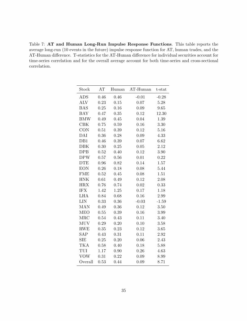
Table 7: AT and Human Long-Run Impulse Response Functions. This table reports theaverage long-run (10 events in the future) impulse response function for AT, human trades, and theAT-Human difference. T-statistics for the AT-Human difference for individual securities account fortime-series correlation and for the overall average account for both time-series and cross-sectionalcorrelation.

Stock AT Human AT-Human t-stat

ADS 0.46 0.46 -0.01 -0.28ALV 0.23 0.15 0.07 5.28BAS 0.25 0.16 0.09 9.65BAY 0.47 0.35 0.12 12.30BMW 0.49 0.45 0.04 1.39CBK 0.75 0.59 0.16 3.30CON 0.51 0.39 0.12 5.16DAI 0.36 0.28 0.09 4.33DB1 0.46 0.39 0.07 6.62DBK 0.30 0.25 0.05 2.12DPB 0.52 0.40 0.12 3.90DPW 0.57 0.56 0.01 0.22DTE 0.96 0.82 0.14 1.57EON 0.26 0.18 0.08 5.44FME 0.52 0.45 0.08 1.51HNK 0.61 0.49 0.12 2.08HRX 0.76 0.74 0.02 0.33IFX 1.42 1.25 0.17 1.18LHA 0.84 0.68 0.16 2.99LIN 0.33 0.36 -0.03 -1.59MAN 0.49 0.36 0.12 3.50MEO 0.55 0.39 0.16 3.99MRC 0.54 0.43 0.11 3.40MUV 0.29 0.20 0.10 3.58RWE 0.35 0.23 0.12 3.65SAP 0.43 0.31 0.11 2.92SIE 0.25 0.20 0.06 2.43TKA 0.58 0.40 0.18 5.88TUI 1.17 0.90 0.26 4.63VOW 0.31 0.22 0.09 8.99Overall 0.53 0.44 0.09 8.71

35

Table 8: Long Run - Short Run Impulse Response. This table reports the long-run impulseresponse (10 events in the future) minus the short-run impulse response (immediate) for AT, humantrades, and the AT-Human difference. T-statistics for the AT-Human difference for individualsecurities account for time-series correlation and for the overall average account for both time-series and cross-sectional correlation.

Stock AT Human AT-Human t-stat

ADS 0.20 0.22 -0.02 -0.59ALV 0.09 0.06 0.03 2.25BAS 0.13 0.07 0.05 8.22BAY 0.22 0.16 0.06 4.57BMW 0.23 0.24 -0.01 -0.95CBK 0.26 0.21 0.04 0.71CON 0.27 0.21 0.06 5.25DAI 0.14 0.09 0.04 2.52DB1 0.21 0.18 0.03 4.38DBK 0.13 0.11 0.02 0.98DPB 0.24 0.16 0.08 4.25DPW 0.16 0.21 -0.05 -1.51DTE 0.00 0.10 -0.10 -1.26EON 0.13 0.08 0.04 3.66FME 0.21 0.17 0.04 0.94HNK 0.24 0.19 0.05 1.08HRX 0.31 0.36 -0.05 -1.17IFX 0.01 0.15 -0.14 -1.16LHA 0.27 0.22 0.05 0.85LIN 0.17 0.20 -0.03 -1.39MAN 0.25 0.20 0.05 1.96MEO 0.26 0.19 0.07 2.83MRC 0.28 0.23 0.05 2.33MUV 0.13 0.09 0.04 2.23RWE 0.17 0.11 0.06 2.59SAP 0.13 0.07 0.06 3.75SIE 0.12 0.10 0.03 1.38TKA 0.23 0.16 0.07 3.56TUI 0.41 0.39 0.02 0.98VOW 0.15 0.10 0.05 5.00Overall 0.19 0.17 0.02 2.76

36

Table 9: AT-Human Variance Decomposition. This table reports the percentage of the vari-ance of the efficient price correlated with AT and human trades. The remainder is in the Returncolumn and is unrelated to trading. AT-Human is the average difference in efficient price varianceexplained by AT and humans. T-statistics for the AT-Human difference for individual securitiesaccount for time-series correlation and for the overall average account for both time-series andcross-sectional correlation.

Stock AT Human Return AT-Human t-stat

ADS 4.01% 4.50% 91.49% -0.49% -1.3ALV 3.81% 2.01% 94.18% 1.80% 4.85BAS 4.18% 1.81% 94.01% 2.37% 9.66BAY 6.08% 3.69% 90.23% 2.39% 8.98BMW 4.05% 3.95% 92.01% 0.10% 0.20CBK 6.24% 4.06% 89.70% 2.18% 2.83CON 5.23% 3.32% 91.45% 1.92% 4.88DAI 4.23% 2.76% 93.01% 1.47% 3.15DB1 6.05% 4.83% 89.12% 1.21% 4.45DBK 4.29% 3.25% 92.46% 1.04% 1.93DPB 4.10% 2.68% 93.23% 1.42% 2.56DPW 4.54% 4.64% 90.82% -0.0% -0.15DTE 12.71% 10.15% 77.13% 2.56% 1.03EON 4.73% 2.51% 92.77% 2.22% 4.98FME 5.06% 3.83% 91.11% 1.22% 1.35HNKp 5.60% 4.70% 89.70% 0.90% 1.09HRX 5.77% 5.42% 88.81% 0.35% 0.4IFX 5.73% 5.67% 88.61% 0.06% 0.04LHA 6.42% 4.52% 89.06% 1.90% 2.76LIN 3.21% 4.01% 92.78% -0.80% -2.42MAN 4.90% 3.01% 92.09% 1.89% 2.70MEO 5.88% 3.31% 90.81% 2.57% 3.17MRC 5.63% 4.11% 90.25% 1.52% 2.38MUV 5.49% 2.89% 91.62% 2.59% 3.85RWE 5.15% 2.56% 92.29% 2.59% 3.17SAP 4.69% 2.76% 92.55% 1.94% 2.46SIE 3.88% 2.76% 93.36% 1.13% 1.88TKA 6.07% 3.28% 90.65% 2.79% 4.52TUI 7.12% 4.93% 87.95% 2.19% 3.67VOW 5.94% 3.24% 90.83% 2.70% 5.68Overall 5.36% 3.84% 90.80% 1.52 % 8.01

37

Table 10: AT and Human Time at Best Quotes. This table reports the number of secondsAT are at the best bid and ask quotes minus the number of seconds human traders are at the bestquotes. The remainder of time both AT and humans are both at the best quotes. The first columnreports the AT - Human difference in time at best quotes. The subsequent columns report theAT-Human difference for time when stocks’ spreads are below their per stock time-series average(Low Spread), when spreads are above their per stock time-series average (High Spread), and theAT-Human difference-in-difference for the low-spread and high-spread times (Low-Spread columnminus High-Spread column). T-statistics for individual securities account for time-series correlationand for the overall average account for both time-series and cross-sectional correlation.

Low Spread High Spreads Low-spread minusStock AT - Human t-stat AT - Human AT - Human High-spread t-stat

ADS 4235 3.91 1454 2780 -1326 -2.35ALV -3000 -2.94 -2368 -632 -1735 -2.67BAS 1011 1.41 -492 1503 -1995 -6.07BAY 3136 6.44 718 2418 -1700 -10.58BMW 6321 4.31 2612 3708 -1095 -1.83CBK 4706 2.95 2996 1709 1287 2.1CON 1249 0.96 -739 1988 -2727 -8.01DAI -3893 -2.27 -3508 -385 -3122 -14.16DB1 2739 4.94 132 2607 -2475 -2.88DBK -3395 -8.58 -3254 -141 -3112 -8.51DPB 7115 7.83 2187 4927 -2740 -6DPW 4555 4.76 2789 1765 1024 2.83DTE -2461 -3.56 -2087 -374 -1713 -3.9EON 1479 2.29 -301 1780 -2081 -5.59FME 11850 11.64 5361 6489 -1128 -0.75HNK 7494 10.04 4054 3439 615 0.58HRX 1028 0.54 -722 1751 -2474 -5.04IFX -201 -0.22 -287 85 -372 -0.95LHA 4056 2.45 3215 840 2375 1.9LIN 7219 12.42 2727 4492 -1764 -4.03MAN 4712 9.18 1297 3415 -2117 -6.42MEO 6843 3.93 3258 3585 -326 -0.53MRC 9155 9.8 3348 5806 -2457 -5.3MUV 6959 8.94 2492 4466 -1974 -2.58RWE 3551 6.13 874 2676 -1802 -2.69SAP 3715 6.1 656 3059 -2402 -6.78SIE -1911 -2.48 -2612 701 -3313 -11.73TKA 4238 14.51 883 3354 -2470 -6.35TUI 5885 5.26 4082 1802 2279 3.16VOW 2415 2.27 -42 2458 -2500 -3.12Overall 3360 7.00 958 2403 -1445 -7.21

38

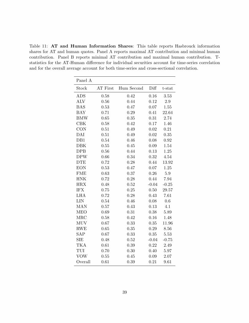
Table 11: AT and Human Information Shares: This table reports Hasbrouck informationshares for AT and human quotes. Panel A reports maximal AT contribution and minimal humancontribution. Panel B reports minimal AT contribution and maximal human contribution. T-statistics for the AT-Human difference for individual securities account for time-series correlationand for the overall average account for both time-series and cross-sectional correlation.

Panel A

Stock AT First Hum Second Diff t-stat

ADS 0.58 0.42 0.16 3.53ALV 0.56 0.44 0.12 2.9BAS 0.53 0.47 0.07 1.55BAY 0.71 0.29 0.41 22.64BMW 0.65 0.35 0.31 2.74CBK 0.58 0.42 0.17 1.46CON 0.51 0.49 0.02 0.21DAI 0.51 0.49 0.02 0.35DB1 0.54 0.46 0.08 0.92DBK 0.55 0.45 0.09 1.54DPB 0.56 0.44 0.13 1.25DPW 0.66 0.34 0.32 4.54DTE 0.72 0.28 0.44 13.92EON 0.53 0.47 0.07 1.25FME 0.63 0.37 0.26 5.9HNK 0.72 0.28 0.44 7.94HRX 0.48 0.52 -0.04 -0.25IFX 0.75 0.25 0.50 29.57LHA 0.72 0.28 0.43 7.61LIN 0.54 0.46 0.08 0.6MAN 0.57 0.43 0.13 4.1MEO 0.69 0.31 0.38 5.89MRC 0.58 0.42 0.16 1.48MUV 0.67 0.33 0.35 11.96RWE 0.65 0.35 0.29 8.56SAP 0.67 0.33 0.35 5.53SIE 0.48 0.52 -0.04 -0.75TKA 0.61 0.39 0.22 2.49TUI 0.70 0.30 0.40 5.97VOW 0.55 0.45 0.09 2.07Overall 0.61 0.39 0.21 9.61

39

Table 11 cont.Panel B

Stock AT Second Hum First Diff t-stat

ADS 0.48 0.52 -0.03 -0.67ALV 0.44 0.56 -0.12 -2.43BAS 0.43 0.57 -0.13 -3.53BAY 0.62 0.38 0.23 8.84BMW 0.57 0.43 0.14 1.04CBK 0.50 0.50 0.01 0.05CON 0.43 0.57 -0.15 -1.75DAI 0.41 0.59 -0.19 -2.36DB1 0.42 0.58 -0.16 -2.44DBK 0.42 0.58 -0.17 -3.35DPB 0.46 0.54 -0.08 -0.79DPW 0.58 0.42 0.17 2.17DTE 0.54 0.46 0.08 1.15EON 0.43 0.57 -0.13 -2.82FME 0.58 0.42 0.16 3.5HNK 0.65 0.35 0.31 5.36HRX 0.41 0.59 -0.18 -1.28IFX 0.64 0.36 0.27 5.51LHA 0.65 0.35 0.29 4.73LIN 0.45 0.55 -0.11 -0.85MAN 0.47 0.53 -0.05 -1.37MEO 0.60 0.40 0.19 3.78MRC 0.50 0.50 -0.01 -0.07MUV 0.58 0.42 0.15 4.47RWE 0.55 0.45 0.09 2.89SAP 0.62 0.38 0.24 3.61SIE 0.41 0.59 -0.18 -3.14TKA 0.56 0.44 0.11 1.3TUI 0.61 0.39 0.21 2.86VOW 0.44 0.56 -0.12 -2.25Overall 0.51 0.49 0.03 1.22

40

Fig

ure

1:C

um

ula

tive

Imp

uls

eR

esp

onse

Fu

nct

ions

for

AT

and

Hu

man

Init

iate

dT

rad

es

41