Algorithmic Composition, illustrated by my own work:

A review of the period 1971-2008

Clarence Barlow Department of Music, University of California Santa Barbara, USA

barlow [at] music [dot] ucsb [dot] edu

Proceedings of Korean Electro-Acoustic Music Society's 2011 Annual Conference (KEAMSAC2011) Seoul, Korea, 22-23 October 2011

Since 1971, marking my first departure from fourteen years of spontaneous composition, my work has been mainly algorithmic in nature. Some of it was generated by single algorithm sets developed for multiple use, the properties of the results deriving from the input. In other cases, the algorithms were used once only, with the dedicated purpose of generating a single work. The algorithms ranged from verbal instructions to complex computer programs.

Of the eighty-odd pieces I have composed since 1971, about a quarter arose from three verbal scores, Textmusic (converting written text into notes), ...until... (working systematically with interval ratios) and Relationships (working with levels of complexity of melody and rhythm in the context of harmony and meter). Another quarter or the pieces were generated by three individual computer programs - TXMS (Textmusic packaged into software), Autobusk (for the generation of MIDI pitch sequences from scales and meters as well as twelve real-time variable parameters such as tonal and metric field strength) and PAPAGEI (for the generation of MIDI events based on patchable live interaction with an improvising performer). Yet another quarter of my compositions since 1971 have resulted from dedicated sets of algorithms for one-time use. Further computer programs such as Synthrumentator and Spectasizer (for the conversion of speech sounds into instrumental scores) were used to generate parts of other compositions.

In this paper I will refer to TXMS, Autobusk and Synthrumentator as well as to two compositions generated by dedicated software, ...or a cherish'd bard... (in which the algorithms generate all aspects of the piece from pitch and rhythm to the overall form) and Approximating Pi (in which algebraically defined algorithms generate the sound waves).

Textmusic

In 1970, the music I composed derived strongly from serial

techniques of composers from Schoenberg to Stockhausen,

dependent on music tradition and evolution. While doing

so, I paused to consider whether it was possible to make

music using concepts exclusively from everyday life. The

result was Textmusic of April 1971, instructions for making

a piano piece. Based on the orthography of a completely

arbitrary text, I structured the linguistic concepts letters,

syllables, words, phrases and sentences, the key-colors

black/white/mixed as well as the physical traits loud/soft,

short/long and (right pedal-) depressed/released:

Take a text consisting of a number of words, phrases, or sentences. Prepare the keys of the piano in the following way: A key somewhere in the middle of the keyboard is marked with the first letter of the chosen text. The next keys of the same color, alternating to left and right (or vice versa) are treated with the succeeding letters in the text; if a certain letter occurs a second time, it should be dropped, and instead the next letter which has not yet occurred taken, until every letter of the text is represented on the keyboard.

This procedure is then repeated with the keys of the other color, and then yet a third time, without taking the color of the keys into consideration.

The text can now be ‘played’ according to the three key-color-systems - and one can 1. play the letters singly, or together as syllables, words, phrases (in their order of appearance in the text) or even an entire sentence – in all cases, the sound should be repeated as often as the number of syllables it contains, 2. change the position of the right pedal (between depressed and released), the loudness (between loud and soft), and the length of the sound (between short and long) at best only at change of syllable, and the key-color at best only at change of word.

Figure 1 exemplifies of the application of these rules to the

text Ping by Samuel Beckett, which begins with the words:

“All known all white bare white body fixed one yard legs

joined like sewn”. The 25 different letters of the text

ALKNOWHITEBRDYFXGSJQUVCMP (the only letter missing

is Z) are assigned in turn to an equal number of black

(pentatonic), white (diatonic) and mixed-color keys

(chromatic). Figure 1 shows at top left and top right how

these 25 letters are allocated chromatically, spanning

exactly two octaves; the score’s opening notes up to

“joined” are also shown. In diatonic allocation, the 25

letters span 3½ octaves, in pentatonic allocation 5 octaves.

Figure 1. How the 25 different letters of Beckett’s Ping are chromatically assigned to the keys of a piano according to the rules outlined in Textmusic. Also shown: the opening of Textmusic Version 6, based on the Beckett text.

Soon after I drew up the rules of Textmusic, I realized that

their algorithmic nature lent itself to incorporation into a

computer program for the automatic generation of

multiple versions of the piece, even following designs by

persons other than myself. Indeed, of the 15 versions that

were realized from 1971 to 1984, a computer program

generated six, of which three were designed by others.

The program in question, written in 1971-72 in Fortran,

was named TXMS (from Textmusic), its input first entered

into an accompanying form chart, shown in Figure 2.

Figure 2. This chart shows fields for entering parameter values for

computer-generating a version of Textmusic. The curves here are for

Version 4, based on the text in the instructional verbal score itself.

TXMS is a stochastic program, generating notes according

to probability values, previously entered as transitions into

the chart shown above (here for Textmusic Version 4), from

where the salient values are read and typed as input. Take

e.g. the uppermost field for the distribution of letters,

syllables, words, phrases and sentences. At the left,

signifying the start of the piece, the probability of single

letters (level 1 or single notes) is 100%. One section later

(1/20

th of the piece, numbered above the chart in fives), the

probability of syllables (level 2), initially at 0%, begins to

increase, that of letters to decrease, until at the end of

section 4 they respectively stand at 70% to 30%. At this

point, the probability of words (level 3) is instantaneously

set at 30%, that of syllables at 40%, that of letters remains

fixed at 30%, values which remain in force till the end of

section 8, where the probability of words jumps to 100%

and stays there till the end of section 10. All through the

process, random numbers – based on the respective

probability – determine whether a single letter is to be

converted to a note, or letters as part of a syllable, word,

phrase or sentence to a chord.

The same system is used for the other parameters color,

loudness, duration and pedal. For instance, at the start of

the piece, the key-color is totally mixed (chromatic),

a random half of the notes is loud and the other half soft,

a random half of the notes is short and the other half long,

and 70% of the events are played with the pedal depressed

and 30% with it released.

Further information required by the chart, not shown here,

are the number of hands, the number of fingers in each

hand(!), the span of each hand measured in white keys, as

well as the expected duration of the short events and that

of the long ones.

There was a dearth of available notation programs in the

early 1970s. I wrote my first one, ЖSC, with notes, replete

with stems and beams, drawn on a plotter and directly

readable by a performer, a bit later, from 1972-76 (the Ж is

a wildcard for the letters K, L and M in the three main

modules “Keyboard reader”, “Lister” and “Music writer”,

and the SC stands for “score”). TXMS’s output was a kind of

staff notation intended instead for regular line printers of

the time, making it relatively easy to copy the music by

hand from the output into a score. The characters used

were [|] for (vertical) staff lines and beams, [0] for note-

heads, [-] for (horizontal) stems, [#] for sharps. By

overprinting, I achieved results like those reconstructed

and shown in Figure 3: an 8th

-note D5-sharp followed by a

16th

-note D5-natural (every accidental applies to the note it

precedes), as read from top to bottom in the treble clef.

Figure 3. A reconstructed example of the printed output of

TXMS with staff, note-heads, stems, beams and accidental.

Autobusk

Harmonicity

In 1975, having left serialism far behind in my work,

I became intrigued by the idea of regarding tonality and

meter, eschewed by serialists, embraced by conservatives,

as physical phenomena manifest as fields of variable

strength: I worked towards music moving in a continuum

ranging from atonal to tonal, from ametric to metric. To

this end, in 1978 I found sufficiently satisfactory algebraic

solutions, exemplified in the field of tonality by formulas

for numerical indigestibility and intervallic harmonicity as

shown in Figure 4 and as tables in Figure 5.

Figure 4. Formulas for the Indigestibility of a natural number and the

Harmonicity of an interval ratio.

Figure 5. Tables for the Indigestibility of a natural number and the

Harmonicity of an interval ratio.

Based on an algebraic evaluation of a quality of natural

numbers based on their size and divisibility, which I call

indigestibility (whereby small primes and their products are

more ‘digestible’ than products containing larger primes),

the formula for the harmonicity of an interval ratio yields

values such as +1.0 for the 1:2 octave, +0.273 for the 2:3

perfect 5th

, -0.214 for the 3:4 perfect 4th

(the negative sign

indicates a polarity to the upper note, here the root of the

interval; a positive polarity signifies a lower-pitched root),

and +0.119 for the major 3rd

4:5 etc., as seen in Figure 5.

With these formulas it was found possible to rationalize

scales known by interval size, e.g. the chromatic scale given

as multiples of 100 cents was rationalized to the values

1:1 15:16 8:9 5:6 4:5 45:32 2:3 5:8 3:5 5:9 8:15 1:2,

a solution that has been known and accepted for centuries.

Any pitch-set known in terms of cents can be similarly

rationalized by the harmonicity algorithms described

above.

Moving on to meter, another set of formulas governs the

metric properties of the music I set out to compose, shown

in Figure 6. Terms I have introduced will next be explained

(the most important of which are Stratification and Metric

Indispensability), along with terms of general usage.

Figure 6. Formulas for Metric Indispensability of pulses in Prime and in

Multiplicative Meters.

A meter is prime, i.e. containing a prime number of equal

time-units (here called pulses) e.g. 2, 3, 5, 7, 11, etc., or

multiplicative, i.e. containing as pulse quantity a product of

primes, e.g. 4, 6, 8, 9, 10, etc. Additive meters (e.g. 3+3+2

pulses = 8) are not covered here. Meters exhibit a certain

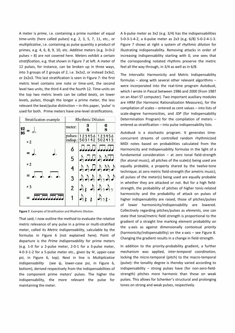
stratification, e.g. that shown in Figure 7 at left. A meter of

12 pulses, for instance, can be broken up in three ways,

into 3 groups of 2 groups of 2, i.e. 3x2x2, or instead 2x3x2,

or 2x2x3. This last stratification is seen in Figure 7: the first

metric level contains one note or time-unit, the second

level two units, the third 4 and the fourth 12. Time-units on

the top two metric levels can be called beats, on lower

levels, pulses, though the longer a prime meter, the less

relevant the beat/pulse distinction – in this paper, ‘pulse’ is

used for both. Prime meters have one-level stratifications.

Figure 7. Examples of Stratification and Rhythmic Dilution.

That said, I now outline the method to evaluate the relative

metric relevance of any pulse in a prime or multi-stratified

meter, called its Metric Indispensability, calculable by the

formulas in Figure 6 (not explained here). Point of

departure is the Prime Indispensability for prime meters

(e.g. 1-0 for a 2-pulse meter, 2-0-1 for a 3-pulse meter,

4-0-3-1-2 for a 5-pulse meter etc., given by Ψ, upper-case

psi, in Figure 6, top). Next in line is Multiplicative

Indispensability (see ψ, lower-case psi, in Figure 6,

bottom), derived respectively from the indispensabilities of

the component prime meters’ pulses. The higher the

indispensability, the more relevant the pulse for

maintaining the meter.

A 6-pulse meter as 3x2 (e.g. 3/4) has the indispensabilities

5-0-3-1-4-2, a 6-pulse meter as 2x3 (e.g. 6/8) 5-0-2-4-1-3.

Figure 7 shows at right a system of rhythmic dilution for

illustrating indispensability. Removing attacks in order of

increasing indispensability starting with 0, one sees that

the corresponding notated rhythms preserve the metric

feel all the way through, in 3/4 as well as in 6/8.

The Intervallic Harmonicity and Metric Indispensability

formulas – along with several other relevant algorithms –

were incorporated into the real-time program Autobusk,

which I wrote in Pascal between 1986 and 2000 (from 1987

on an Atari ST computer). Two important auxiliary modules

are HRM (for Harmonic Rationalization Measures), for the

compilation of scales – entered as cent values – into lists of

scale-degree harmonicities, and IDP (for Indispensability

Determination Program) for the compilation of meters –

entered as stratification – into pulse indispensability lists.

Autobusk is a stochastic program. It generates time-

concurrent streams of controlled random rhythmicized

MIDI notes based on probabilities calculated from the

Harmonicity and Indispensability formulas in the light of a

fundamental consideration – at zero tonal field-strength

(for atonal music), all pitches of the scale(s) being used are

equally probable, a property shared by the twelve-tone

technique; at zero metric field-strength (for ametric music),

all pulses of the meter(s) being used are equally probable

in whether they are attacked or not. But for a high field-

strength, the probability of pitches of higher tonic-related

harmonicity and the probability of attack on pulses of

higher indispensability are raised, those of pitches/pulses

of lower harmonicity/indispensability are lowered.

Collectively regarding pitches/pulses as elements, one can

state that tonal/metric field strength is proportional to the

gradient of a straight line marking element probability on

the y-axis as against dimensionally contextual priority

(harmonicity/indispensability) on the x-axis – see Figure 8.

Changing the gradient results in a change in field-strength.

In addition to the priority-probability gradient, a further

mechanism was applied, inter-temporal coordination,

locking the micro-temporal (pitch) to the macro-temporal

(pulse): the tonality degree is thereby varied according to

indispensability – strong pulses have (for non-zero-field-

strength) pitches more harmonic than those on weak

pulses. This allows for Schenker’s structural and prolonging

tones on strong and weak pulses, respectively.

Figure 8. A straight line showing probability as a function of priority, the

gradient as a function of field-strength.

Autobusk receives as input a list of scales and meters (pre-

compiled by HRM and IDP, extensions .HRM and .IDP), and

most likely a parameter score (extension .PRK) containing

time-tagged values for 12 parameters, seen accordingly

numbered in the screen shot in Figure 9: “metriclarity” and

“harmoniclarity” mean the metric and tonal field-strength.

If the event of the absence of a .PRK file, user-defined

preset (or else default) parameter values are used.

Figure 9. Screen-shot of Autobusk.

Parameters can be changed in real-time by key-typing, the

mouse, a MIDI input device such as a keyboard and/or

time-tagged instructions in a .PRK file. The output, usually

MIDI notes, is sent to the MIDI port and/or to a file. The

program is freely downloadable at Mainz University

<http://www.musikwissenschaft.uni-mainz.de/Autobusk/>,

ready to be run on an Atari, should one have one, together

with a pdf user manual. In order to run it in Windows, one

needs an Atari emulator, as indicated by the site. For use

on a Macintosh, an additional Windows emulator is

necessary.

Synthrumentator

In 1981, while planning a new work for chamber ensemble,

I had the idea of writing a spectral piece in which the

overall sound of the ensemble would reflect the sounds of

speech. For this I would convert a spectral analysis of

spoken words into a playable score for nearly pure tones,

e.g. string harmonics. Playing the score engenders the

synthesis of harmonic spectra, for which the best phoneme

types are vowels, approximants, laterals and nasals (thus

excluding plosives, fricatives and trills).

For the envisaged composition, I put together nine

nonsensical but grammatically correct German sentences

based on words consisting solely of these harmonically

synthesizable phonemes - of the languages I was familiar

with at that time, German seemed especially suitable due

to its systematic phonetic spelling as an aid in looking for

usable words. These sentences – the title of the piece, Im

Januar am Nil, was taken from one of them – were Fourier-

analyzed and the results converted into something like a

MIDI file (this work predated MIDI by three years): every

set of six Fourier time-windows was merged into an chord

consisting of overtones, each with its pertinent amplitude,

as later with pitch and velocity in a MIDI file.

The really significant follow-up to this procedure was the

subsequent re-setting of all amplitudes to multiples of an

arbitrary amplitude, termed the amplitude tolerance: any

partial in one chord having the same altered amplitude as

the identical partial in the following chord is sonically

connected to that partial, i.e. it is not repeated but held.

More on this procedure – termed calming – later.

Figure 10 shows (above) the words in Armenien scored for

bass clarinet playing the fundamental and for seven strings

playing the partials and (below) a graphic representation of

the same, which strongly resembles the sonagram of the

spoken words. I called this technique Synthrumentation,

from “synthesis by instrumentation”. From 1981 till the

completion of the piece in 1982 and that of its final revised

version in 1984, I wrote all the software, from the Fourier

analysis to the generation of the score, a total of twenty

programs in Fortran. The output was printed using my

notation program ЖSC, mentioned above, on a 9-pin dot-

matrix printer.

Figure 10. Synthrumentation of the words in Armenien in the chamber

ensemble piece Im Januar am Nil: compact score (above) and graphic

representation of the score (below).

In the course of the years, I used synthrumentation for a

number of pieces, prompting me to combine all modules

into a single Linux GNU Pascal program for repeated use

named Synthumentator. In principle, the procedure is the

same: a Fourier analysis of a sound wave is converted to a

MIDI file of chords comprising partials of the fundamental

analysis frequency (my favorite: 49 Hz, almost exactly G2,

and a whole-number subdivision of the sampling rate

44,100 Hz). This conversion maps frequencies to MIDI

notes, maps amplitudes to velocity.

Finally the MIDI file is calmed. For instance, with a

tolerance (now called velocity tolerance) of 4, all velocities

are re-set to multiples of 4, i.e. 0, 4, 8, 12 etc. Notes now

with velocity 0 are removed. If a particular note in any one

chord, say G4, has the same adjusted velocity, say 64, as

the G4 in the next chord, the note-off of the first chord and

the note-on of the second are removed, lengthening the

former. The higher the velocity tolerance, the smaller and

sparser the resulting output file. A low velocity tolerance

will result in a dense output file, perhaps obscuring the

desired timbral link to the sound source. The main task in

using this program is to find the optimal velocity tolerance.

The program is being currently rewritten in C for Mac OS

and Windows.

...or a cherish'd bard...

In 1998 I decided to write a solo piece for the pianist

Deborah Richards in order to commemorate her 50th

birthday. A common means of honoring a person in a music

score is to take those letters of the person’s name which

are available as note names (i.e. A-G in English, with the

additional H and S in German) and to use these notes

repeatedly. In fortunate cases like ABEGG and BACH, the

complete names are available as notes. However, before

discarding the idea of using Ms Richards’ name in this way,

I noticed that in her first name, the letters DEB and AH

were definitely usable as notes in German, and that the

intervening letters OR denote a logical operation. Further,

DEB belong to a whole-tone scale (B is German for B-flat)

and AH (H is German for B-natural) belong to the other

whole-tone scale. Finally I also noticed that the letters DEB

and A are digits in the hexadecimal number system.

I accordingly set up two pitch-chains in the two whole-tone

scales, one chaining transpositions of DEB and the other

transpositions of AH – see Figure 11 (top). In theory, each

chain moves in pitch and time to and from ±infinity. Next I

converted the hex numbers DEB and A to their binary

equivalents 1101 1110 1011 and 1010. These became the

repeatable rhythmic cycles in Figure 11 (center): 1 = attack,

0 = silence – the H in AH, not a number, was added as a

silence 0000. Combining the pitch chains and the rhythms, I

obtained the rhythmicized pitch chains shown in Figure 11

(bottom).

Figure 11. Pitch chains, rhythmic cycles and both based on DEB and AH.

After this I set up 120 DEB and, separately, 120 AH

rhythmic chains successively and parallel to each other,

such that all transections of D4 (Middle D) are time-

equidistant at intervals of four seconds, i.e. on the first

beat of every bar from 1 to 120.

Figure 12 shows an example of this procedure as applied to

the infinite DEB chain. The x-axis marks the 120 bars of the

piece, the y-axis a range of 40 octaves from 0.28 μHz to

308 MHz (!). The middle horizontal line marks D4 at 293.67

Hz. Instead of crossing this line every bar, as in the piece,

this graph shows for reasons of space a crossing every 10

bars. The basic DEB motif, both in pitch and rhythm, is

displayed in a small box at upper left – the entire graph

consists of chains of this motif, reduced to 50% in size.

Figure 12. Parallel DEB chains crossing D4 downwards every ten bars (in

the piece this happens every bar).

To change this static scenario into a dynamic one, I then

made the gradient of the chains successively increase with

time, forming primordial DEB and AH scores.

Next followed the containment of the piece within a

triangular pitch filter, starting at the beginning (left) at a

width of zero half-steps centered on D4, gradually

expanding, the width at any bar in half-steps equalling the

bar number, reaching a range of 10 octaves at bar 120

(right). Obviously the range transcends that of the piano at

around bar 88; the printed score nonetheless contains

notes extending beyond. The result for the DEB score is

displayed as a graph in Figure 13.

Figure 13. The DEB score with increasing chain gradients and triangular

pitch filter.

The final step was a transition in time from the filtered DEB

score to the filtered AH score by means of random

selection – at the start of the piece, the choice of a note

from the DEB score is 100% probable, that of a note from

the AH score 0%. At the end, the probabilities are reversed,

so that in the middle, at bar 60, both scores are subjected

to a 50% probability each. Thus every note of the piece is

taken either from the DEB score or from the AH score:

DEB OR AH, moving from the former to the latter. As a

consequence, the music of the opening bars is in the

whole-tone scale containing DEB, that in bar 60 is highly

chromatic with all twelve notes in every octave, and the

final notes are in the other whole-tone scale containing AH.

The whole composition was made by once-used software.

Due to the rising gradients, the resulting durational values

were of an irrational nature. I rationalized the score with

my program Tupletizer, converting irrational time-values to

notatable tuplets by rounding within flexible constraints

and with controllable error. Figure 14 shows bars 92-94 as

notated in Sibelius: the diamond-shaped and crossed note-

heads are an octave higher/lower than written, the former

still within the piano range and the latter beyond.

Figure 14. An excerpt from the Sibelius-printed score.

The title “...or a cherish’d bard...” is an anagram of the

name Deborah Richards. Here is the dedication:

Full fifty years, the most whereof well spent / In service of the Muse, wherefore I pray / That Lady Fortune add three score and ten. / Yet I, a clown cerebral*, so some say, / Unfit in words, resort to music’s way / To help submit my prayer in this regard – / Meseems a minstrel, or a cherish’d bard / Would better wield in verse his worthy pen. *an anagram of the name Clarence Barlow

Approximating Pi

In 2007 my attention was drawn by my colleague Curtis

Roads to the series π = 4(1 – 1/3 +

1/5 –

1/7 +

1/9 ∙∙∙),

something I had not thought about since my school days.

Almost immediately, an electronic music installation began

to shape in my mind, in which the amplitudes of ten

partials of a complex tone would reflect the first ten digits

of the progressive stages of convergence – with each

added component of the series – toward the final value. In

May 2008, the installation, Approximating Pi, which I

realized wholly in Linux GNU Pascal, was given its premiere.

For each convergence, I decided on a time frame of 5040

samples, i.e. 8¾ frames per second. All time frames contain

a set of ten partials of an overtone series, multiples of the

frequency 8¾ Hz, which automatically results from the

width of the frame, 5040 samples. The reason for this

number of samples is that is can be neatly divided into 2 to

10 exactly equal segments, corresponding to the partials

(half this value, 2520, which as least common multiple of

the numbers 1-10 is amenable to the same, corresponds to

17½ frames per second, too fast for my purposes).

The partials are square waves of amplitude 2 raised to the

power of the nth

digit in the decimal representation of the

convergence. In the case 3.14159..., for instance, the

amplitudes of the ten partials are 23, 2

1, 2

4, 2

1 ,2

5, 2

9 etc.

The amplitudes are then rescaled by a multiplication by the

arbitrary factor 2π

/n, forming the envelope of a sawtooth

spectrum, where 'n' is still the partial number.

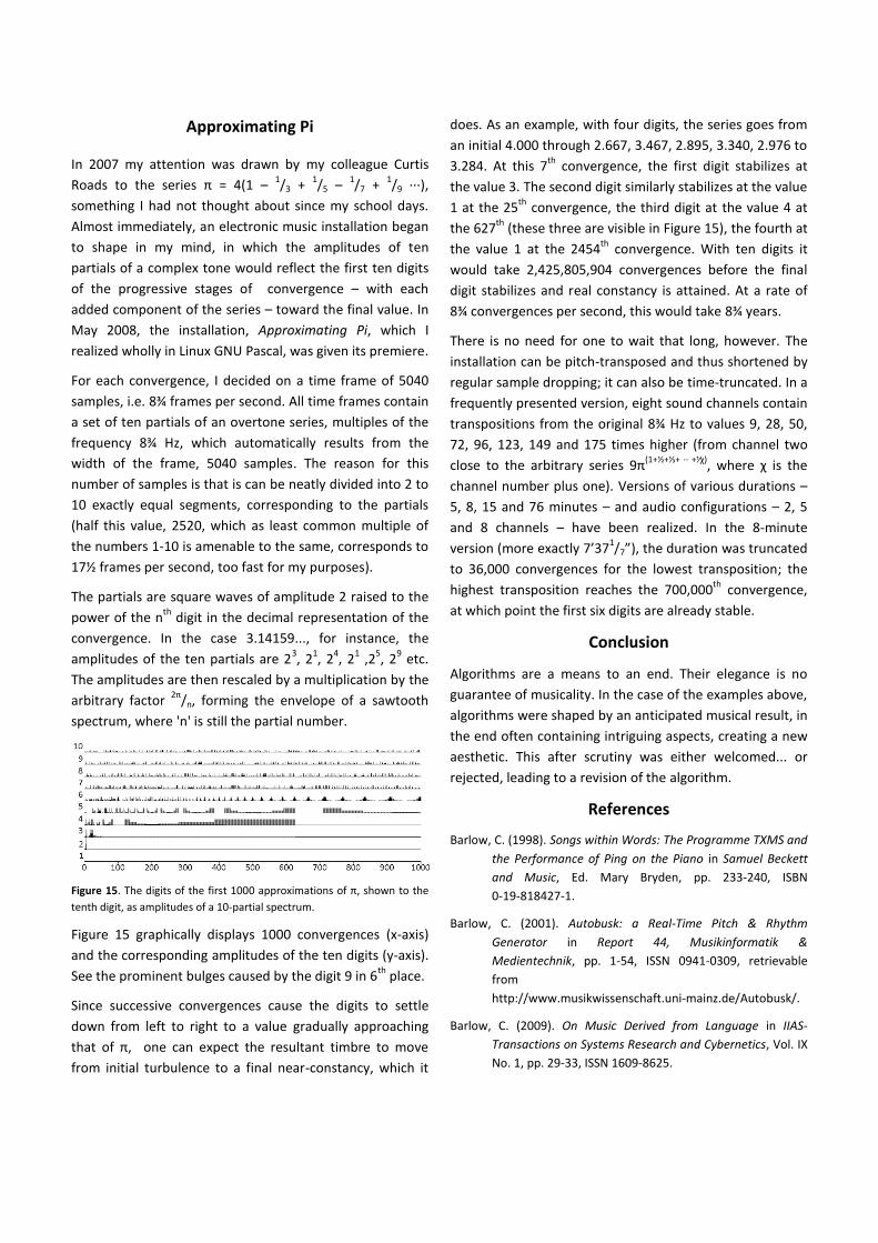
Figure 15. The digits of the first 1000 approximations of π, shown to the

tenth digit, as amplitudes of a 10-partial spectrum.

Figure 15 graphically displays 1000 convergences (x-axis)

and the corresponding amplitudes of the ten digits (y-axis).

See the prominent bulges caused by the digit 9 in 6th

place.

Since successive convergences cause the digits to settle

down from left to right to a value gradually approaching

that of π, one can expect the resultant timbre to move

from initial turbulence to a final near-constancy, which it

does. As an example, with four digits, the series goes from

an initial 4.000 through 2.667, 3.467, 2.895, 3.340, 2.976 to

3.284. At this 7th

convergence, the first digit stabilizes at

the value 3. The second digit similarly stabilizes at the value

1 at the 25th

convergence, the third digit at the value 4 at

the 627th

(these three are visible in Figure 15), the fourth at

the value 1 at the 2454th

convergence. With ten digits it

would take 2,425,805,904 convergences before the final

digit stabilizes and real constancy is attained. At a rate of

8¾ convergences per second, this would take 8¾ years.

There is no need for one to wait that long, however. The

installation can be pitch-transposed and thus shortened by

regular sample dropping; it can also be time-truncated. In a

frequently presented version, eight sound channels contain

transpositions from the original 8¾ Hz to values 9, 28, 50,

72, 96, 123, 149 and 175 times higher (from channel two

close to the arbitrary series 9π(1+½+⅓+ ∙∙ +⅟χ)

, where χ is the

channel number plus one). Versions of various durations –

5, 8, 15 and 76 minutes – and audio configurations – 2, 5

and 8 channels – have been realized. In the 8-minute

version (more exactly 7’371/7”), the duration was truncated

to 36,000 convergences for the lowest transposition; the

highest transposition reaches the 700,000th

convergence,

at which point the first six digits are already stable.

Conclusion

Algorithms are a means to an end. Their elegance is no

guarantee of musicality. In the case of the examples above,

algorithms were shaped by an anticipated musical result, in

the end often containing intriguing aspects, creating a new

aesthetic. This after scrutiny was either welcomed... or

rejected, leading to a revision of the algorithm.

References

Barlow, C. (1998). Songs within Words: The Programme TXMS and

the Performance of Ping on the Piano in Samuel Beckett

and Music, Ed. Mary Bryden, pp. 233-240, ISBN

0-19-818427-1.

Barlow, C. (2001). Autobusk: a Real-Time Pitch & Rhythm

Generator in Report 44, Musikinformatik &

Medientechnik, pp. 1-54, ISSN 0941-0309, retrievable

from

http://www.musikwissenschaft.uni-mainz.de/Autobusk/.

Barlow, C. (2009). On Music Derived from Language in IIAS-

Transactions on Systems Research and Cybernetics, Vol. IX

No. 1, pp. 29-33, ISSN 1609-8625.