Algorithm Theory WS Fabian Kuhn - ac.informatik.uni...

Chapter 6Randomization

Algorithm TheoryWS 2012/13

Fabian Kuhn

Algorithm Theory, WS 2012/13 Fabian Kuhn 2

RandomizationRandomized Algorithm:• An algorithm that uses (or can use) random coin flips in order

to make decisions

We will see: randomization can be a powerful tool to• Make algorithms faster• Make algorithms simpler• Make the analysis simpler

– Sometimes it’s also the opposite…

• Allow to solve problems (efficiently) that cannot be solved (efficiently) without randomization– True in some computational models (e.g., for distributed algorithms)– Not clear in the standard sequential model


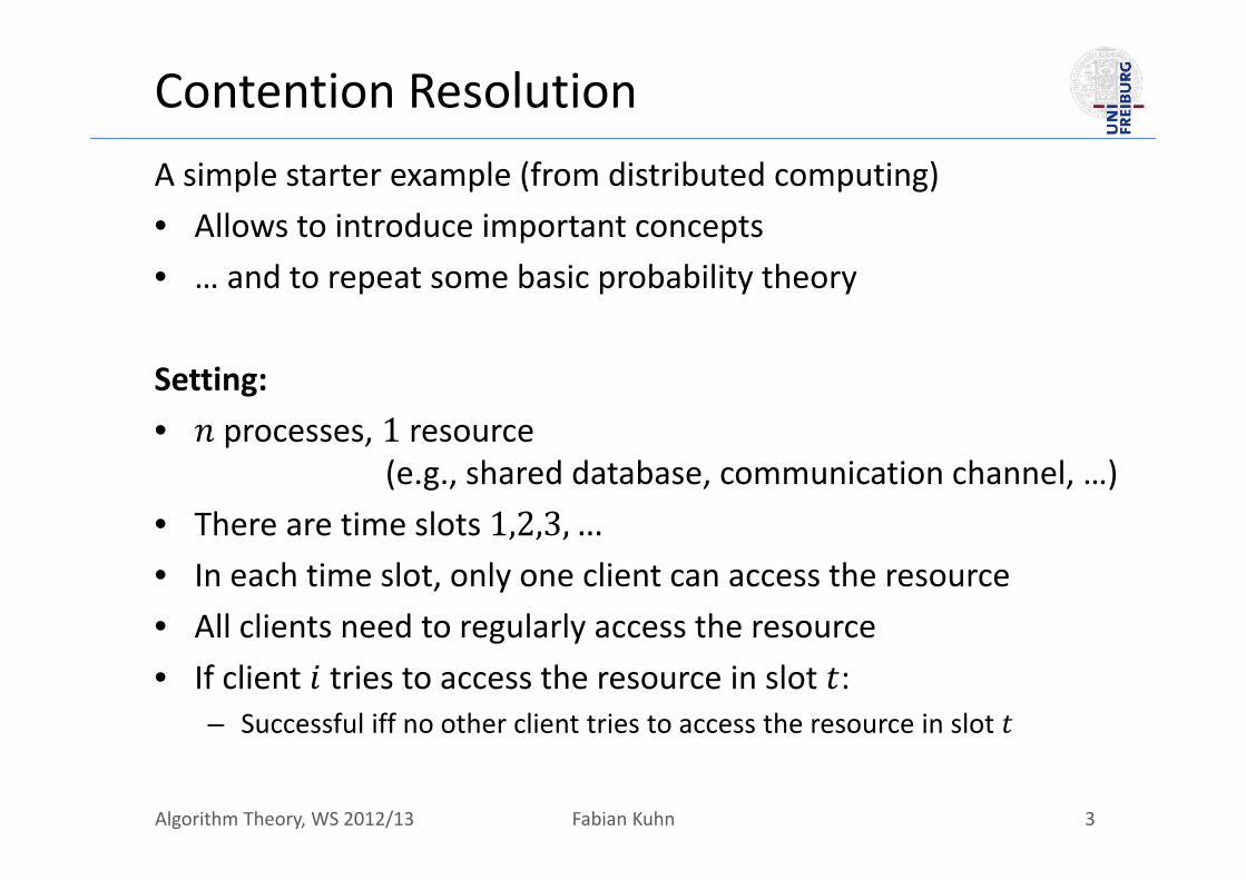
Contention ResolutionA simple starter example (from distributed computing)• Allows to introduce important concepts• … and to repeat some basic probability theory

Setting: • processes, 1 resource

(e.g., shared database, communication channel, …)• There are time slots 1,2,3, …• In each time slot, only one client can access the resource• All clients need to regularly access the resource• If client tries to access the resource in slot :

– Successful iff no other client tries to access the resource in slot


AlgorithmAlgorithm Ideas:• Accessing the resource deterministically seems hard

– need to make sure that processes access the resource at different times– or at least: often only a single process tries to access the resource

• Randomized solution:In each time slot, each process tries with probability .

Analysis:• How large should be?• How long does it take until some process succeeds?• How long does it take until all processes succeed?• What are the probabilistic guarantees?


AnalysisEvents:• , : process tries to access the resource in time slot

– Complementary event: ,

ℙ , , ℙ , 1

• , : process is successful in time slot

, , ∩ ,

• Success probability (for process ):


Fixing • ℙ , 1 is maximized for

⟹ ℙ ,1

11

.

• Asymptotics:

For 2:14 1

1 11

1 12

• Success probability:

ℙ ,


Time Until First SuccessRandom Variable :• if proc. is successful in slot for the first time

• Distribution:

• is geometrically distributed with parameter

ℙ ,1

11 1

.

• Expected time until first success:


Time Until First SuccessFailure Event , : Process does not succeed in time slots 1,… ,

• The events , are independent for different :

ℙ , ℙ , ℙ , 11

11

• We know that ℙ , ⁄ :

ℙ , 11


Time Until First Success

No success by time : ℙ ,⁄

: ℙ , ⁄

• Generally if Θ : constant success probability

⋅ ⋅ ln : ℙ , ⋅ ⁄

• For success probability 1 ⁄ , we need Θ log .

• We say that succeeds with high probability in log time.


Time Until All Processes SucceedEvent : some process has not succeeded by time

,

Union Bound: For events , … , ,

ℙ ℙ

Probability that not all processes have succeeded by time :

ℙ ℙ , ℙ , ⋅ .


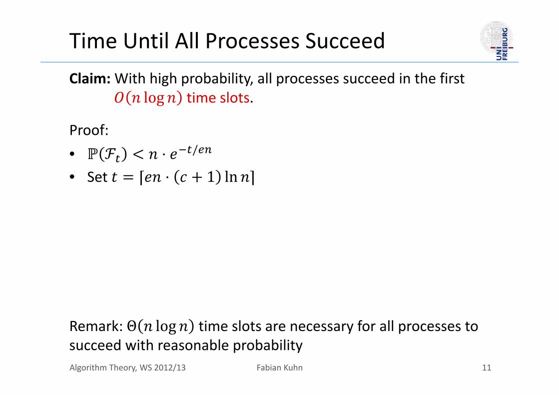
Time Until All Processes SucceedClaim: With high probability, all processes succeed in the first

log time slots.

Proof:• ℙ ⋅ /

• Set ⋅ 1 ln

Remark: Θ log time slots are necessary for all processes to succeed with reasonable probability


Primality TestingProblem: Given a natural number 2, is a prime number?

Simple primality test:

1. if is even then2. return 23. for ≔ 1 to 2⁄ do4. if 2 1 divides then5. return false6. return true

• Running time:


A Better Algorithm?• How can we test primality efficiently?• We need a little bit of basic number theory…

Square Roots of Unity: In ∗ , where is a prime, the only solutions of the equation ≡ 1 mod are ≡ 1 mod

• If we find an ≢ 1 mod such that ≡ 1 mod , we can conclude that is not a prime.


Algorithm IdeaClaim: Let 2 be a prime number such that 1 2 for an integer 0 and some odd integer 3. Then for all ∈ ∗ ,

≡ 1 mod ≡ 1 mod forsome0 .

Proof:• Fermat’s Little Theorem: Given a prime number ,

∀ ∈ ∗ : ≡ 1 mod


Primality TestWe have: If is an odd prime and 1 2 for an integer 0and an odd integer 3. Then for all ∈ 1,… , 1 ,

≡ 1 mod ≡ 1 mod forsome0 .

Idea: If we find an ∈ 1,… , 1 such that

≢ 1 mod ≢ 1 mod forall0 ,we can conclude that is not a prime.

• For every odd composite 2, at least ⁄ of all possible satisfy the above condition

• How can we find such a witness efficiently?


Miller‐Rabin Primality Test• Given a natural number 2, is a prime number?

Miller‐Rabin Test:1. if is even then return 22. compute , such that 1 2 ;3. choose ∈ 2,… , 2 uniformly at random;4. ≔ mod ;5. if 1 or 1 then return true;6. for ≔ 1 to 1 do7. ≔ mod ;8. if 1 then return true;9. return false;


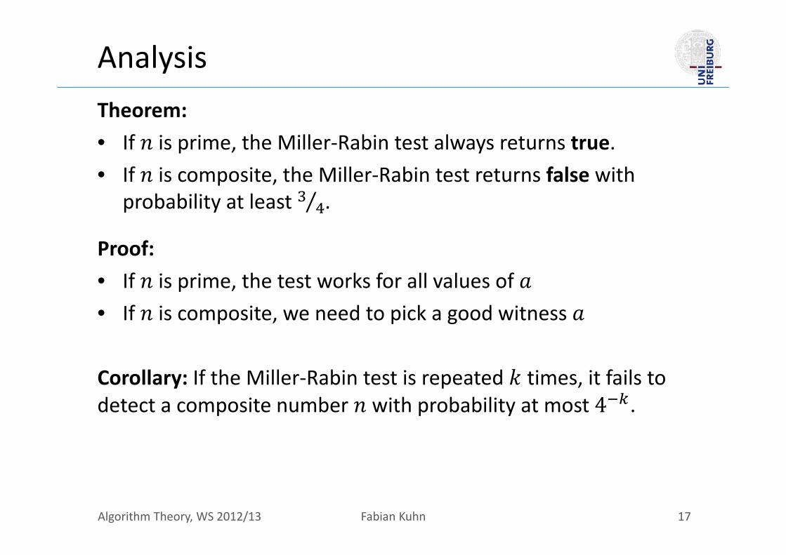
AnalysisTheorem: • If is prime, the Miller‐Rabin test always returns true.• If is composite, the Miller‐Rabin test returns false with

probability at least ⁄ .

Proof:• If is prime, the test works for all values of • If is composite, we need to pick a good witness

Corollary: If the Miller‐Rabin test is repeated times, it fails to detect a composite number with probability at most 4 .


Running TimeCost of Modular Arithmetic:• Representation of a number ∈ : log bits

• Cost of adding two numbers mod :

• Cost of multiplying two numbers ⋅ mod :– It’s like multiplying degree log polynomials use FFT to compute ⋅


Running TimeCost of exponentiation mod :• Can be done using log multiplications

• Base‐2 representation of : ∑ 2

• Fast exponentiation:1. ≔ 1;2. for ≔ log to 0 do3. ≔ mod ;4. if 1 then ≔ ⋅ mod ;5. return ;

• Example: 22 10110


Running TimeTheorem: One iteration of the Miller‐Rabin test can be implemented with running time log ⋅ log log ⋅ log log log .

1. if is even then return 22. compute , such that 1 2 ;3. choose ∈ 2,… , 2 uniformly at random;4. ≔ mod ;5. if 1 or 1 then return true;6. for ≔ 1 to 1 do7. ≔ mod ;8. if 1 then return true;9. return false;


Deterministic Primality Test• If a conjecture called the generalized Riemann hypothesis (GRH)

is true, the Miller‐Rabin test can be turned into a polynomial‐time, deterministic algorithm

It is then sufficient to try all ∈ 1,… , log

• It has long not been proven whether a deterministic, polynomial‐time algorithm exist

• In 2002, Agrawal, Kayal, and Saxena gave an log ‐time deterministic algorithm– Has been improved to log

• In practice, the randomized Miller‐Rabin test is still the fastest algorithm


Randomized QuicksortQuicksort:

function Quick ( : sequence): sequence;

{returns the sorted sequence }begin

if # 1 then returnelse { choose pivot element in ;

partition into ℓ with elements ,and with elements return

end;

ℓ

Quick( ℓ) Quick( )


Randomized Quicksort AnalysisRandomized Quicksort: pick uniform random element as pivot

Running Time of sorting elements:• Let’s just count the number of comparisons• In the partitioning step, all 1 non‐pivot elements have to be

compared to the pivot

• Number of comparisons:

#

• If rank of pivot is :recursive calls with and elements


Randomized Quicksort AnalysisRandom variables:• : total number of comparisons (for a given array of length )• : rank of first pivot• ℓ, : number of comparisons for the 2 recursive calls

1 ℓ

Law of Total Expectation:

ℙ ⋅ |

ℙ ⋅ 1 ℓ |


Randomized Quicksort AnalysisWe have seen that:

ℙ ⋅ 1 ℓ |

Define:• : expected number of comparisons when sorting elements

ℓ 1

Recursion:

⋅


Randomized Quicksort AnalysisTheorem: The expected number of comparisons when sorting elements using randomized quicksort is 2 ln .Proof:

1⋅ 1 1 , 0 0



14⋅ ln

ln ln2 4ln ln2 4


Alternative AnalysisArray to sort: [ 7 , 3 , 1 , 10 , 14 , 8 , 12 , 9 , 4 , 6 , 5 , 15 , 2 , 13 , 11 ]

Viewing quicksort run as a tree:


Comparisons• Comparisons are only between pivot and non‐pivot elements• Every element can only be the pivot once:

every 2 elements can only be compared once!

• W.l.o.g., assume that the elements to sort are 1,2,… ,• Elements and are compared if and only if either or is a

pivot before any element : is chosen as pivot– i.e., iff is an ancestor of or is an ancestor of

ℙ comparison betw. and2

1


Counting ComparisonsRandom variable for every pair of elements , :

1, ifthereisacomparisonbetween and0, otherwise

Number of comparisons:

• What is ?


Randomized Quicksort AnalysisTheorem: The expected number of comparisons when sorting elements using randomized quicksort is 2 ln .Proof:• Linearity of expectation:

For all random variables , … , and all , … , ∈ ,

.



21

1 21


Types of Randomized AlgorithmsLas Vegas Algorithm:• always a correct solution• running time is a random variable

• Example: randomized quicksort, contention resolution

Monte Carlo Algorithm:• probabilistic correctness guarantee (mostly correct)• fixed (deterministic) running time

• Example: primality test


Minimum CutReminder: Given a graph , , a cut is a partition ,of such that ∪ , ∩ ∅, , ∅

Size of the cut , : # of edges crossing the cut• For weighted graphs, total edge weight crossing the cut

Goal: Find a cut of minimal size (i.e., of size )

Maximum‐flow based algorithm:• Fix , compute min ‐ ‐cut for all

• ⋅ per ‐ cut

• Gives an O ‐algorithm

Best‐known deterministic algorithm: log


Edge Contractions• In the following, we consider multi‐graphs that can have

multiple edges (but no self‐loops)

Contracting edge , :• Replace nodes , by new node • For all edges , and , , add an edge ,• Remove self‐loops created at node

not okok

,contract ,


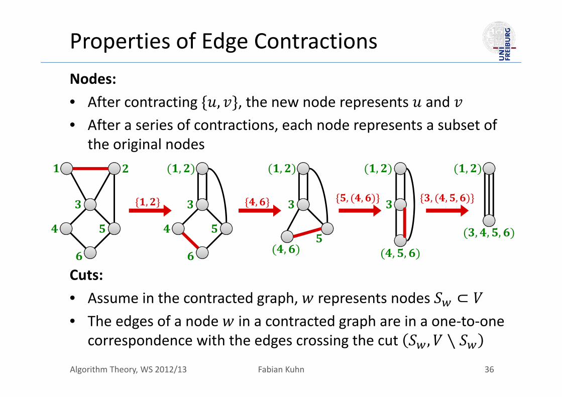
Properties of Edge ContractionsNodes:• After contracting , , the new node represents and • After a series of contractions, each node represents a subset of

the original nodes

Cuts:• Assume in the contracted graph, represents nodes ⊂• The edges of a node in a contracted graph are in a one‐to‐one

correspondence with the edges crossing the cut , ∖

, ,

,

,

, ,

,

, , ,

, , , , , , ,


Randomized Contraction AlgorithmAlgorithm:

while there are 2 nodes docontract a uniformly random edge

return cut induced by the last two remaining nodes(cut defined by the original node sets represented by the last 2 nodes)

Theorem: The random contraction algorithm returns a minimum cut with probability at least 1⁄ .• We will show this next.

Theorem: The random contraction algorithm can be implemented in time .• There are 2 contractions, each can be done in time .• You will show this in the exercises.


Contractions and CutsLemma: If two original nodes , ∈ are merged into the same node of the contracted graph, there is a path connecting and in the original graph s.t. all edges on the path are contracted.

Proof:• Contracting an edge , merges the node sets represented by

and and does not change any of the other node sets.

• The claim the follows by induction on the number of edge contractions.


Contractions and CutsLemma: During the contraction algorithm, the edge connectivity (i.e., the size of the min. cut) cannot get smaller.

Proof:• All cuts in a (partially) contracted graph correspond to cuts of

the same size in the original graph as follows:– For a node of the contracted graph, let be the set of original nodes

that have been merged into (the nodes that represents)– Consider a cut , of the contracted graph– , with

≔∈

, ≔∈

is a cut of .– The edges crossing cut , are in one‐to‐one correspondence with the

edges crossing cut , .


Contraction and CutsLemma: The contraction algorithm outputs a cut , of the input graph if and only if it never contracts an edge crossing , .

Proof:1. If an edge crossing , is contracted, a pair of nodes ∈ ,

∈ is merged into the same node and the algorithm outputs a cut different from , .

2. If no edge of , is contracted, no two nodes ∈ , ∈end up in the same contracted node because every path connecting and in contains some edge crossing ,

In the end there are only 2 sets output is ,


Getting The Min CutTheorem: The probability that the algorithm outputs a minimum cut is at least 2 1⁄ .

To prove the theorem, we need the following claim:

Claim: If the minimum cut size of a multigraph (no self‐loops) is , has at least 2⁄ edges.

Proof:• Min cut has size ⟹ all nodes have degree

– A node of degree gives a cut , ∖ of size

• Number of edges ⁄ ⋅ ∑ deg


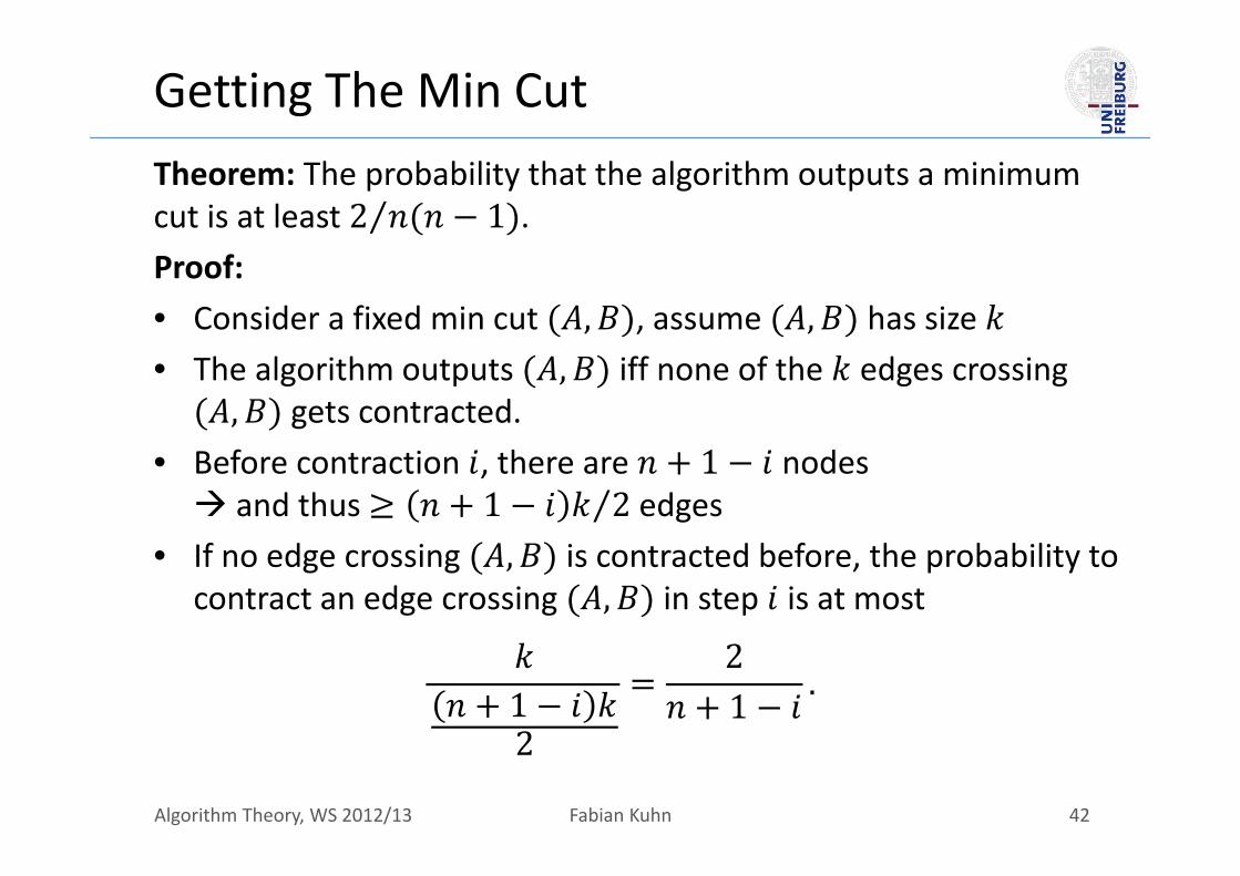
Getting The Min CutTheorem: The probability that the algorithm outputs a minimum cut is at least 2 1⁄ .Proof:• Consider a fixed min cut , , assume , has size • The algorithm outputs , iff none of the edges crossing

, gets contracted.• Before contraction , there are 1 nodes and thus 1 2⁄ edges

• If no edge crossing , is contracted before, the probability to contract an edge crossing , in step is at most

12

21 .


Getting The Min CutTheorem: The probability that the algorithm outputs a minimum cut is at least 2 1⁄ .Proof:• If no edge crossing , is contracted before, the probability to

contract an edge crossing , in step is at most ⁄ .

• Event : edge contracted in step is not crossing ,


Getting The Min CutTheorem: The probability that the algorithm outputs a minimum cut is at least 2 1⁄ .Proof:• ℙ | ∩ ⋯∩ ⁄• No edge crossing , contracted: event ⋂


Randomized Min Cut AlgorithmTheorem: If the contraction algorithm is repeated logtimes, one of the log instances returns a min. cut w.h.p.

Proof:

• Probability to not get a minimum cut in ⋅ 2 ⋅ ln iterations:

11

2

⋅ ⋅ 1

Corollary: The contraction algorithm allows to compute a minimum cut in log time w.h.p.• Each instance can be implemented in time.

( time per contraction)


Can We Do Better?• Time log is not very spectacular, a simple max flow

based implementation has time .

However, we will see that the contraction algorithm is nevertheless very interesting because:

1. The algorithm can be improved to beat every known deterministic algorithm.

1. It allows to obtain strong statements about the distribution of cuts in graphs.


Better Randomized AlgorithmRecall:• Consider a fixed min cut , , assume , has size • The algorithm outputs , iff none of the edges crossing

, gets contracted.• Throughout the algorithm, the edge connectivity is at least

and therefore each node has degree • Before contraction , there are 1 nodes and thus at

least 1 2⁄ edges• If no edge crossing , is contracted before, the probability

to contract an edge crossing , in step is at most

12

21 .


Improving the Contraction Algorithm• For a specific min cut , , if , survives the first

contractions,

ℙ edgecrossing , incontraction 12

.

• Observation: The probability only gets large for large

• Idea: The early steps are much safer than the late steps.Maybe we can repeat the late steps more often than the early ones.


Safe Contraction PhaseLemma: A given min cut , of an ‐node graph survives the first 1 contractions, with probability ⁄ .

Proof:• Event : cut , survives contraction • Probability that , survives the first contractions:


Better Randomized AlgorithmLet’s simplify a bit:

• Pretend that / 2 is an integer (for all we will need it).• Assume that a given min cut survives the first

contractions with probability ⁄ .

, :• Starting with ‐node graph , perform edge contractions

such that the new graph has nodes.

:

1. ≔ mincut contract , 2⁄ ;


3. return min , ;


Success Probability:



3. return min , ;

: probability that the above algorithm returns a min cut whenapplied to a graph with nodes.

• Probability that is a min cut

Recursion:


Success ProbabilityTheorem: The recursive randomized min cut algorithm returns a minimum cut with probability at least 1 log⁄ .

Proof (by induction on ):

214 ⋅ 2

, 2 1


Running Time



3. return min , ;

Recursion:• : time to apply algorithm to ‐node graphs

• Recursive calls: 2

• Number of contractions to get to nodes:

22

, 2 1


Running TimeTheorem: The running time of the recursive, randomized min cut algorithm is log .

Proof:• Can be shown in the usual way, by induction on

Remark:• The running time is only by an log ‐factor slower than

the basic contraction algorithm.• The success probability is exponentially better!


Number of Minimum Cuts• Given a graph , how many minimum cuts can there be?

• Or alternatively: If has edge connectivity , how many ways are there to remove edges to disconnect ?

• Note that the total number of cuts is large.


Number of Minimum CutsExample: Ring with nodes

• Minimum cut size: 2

• Every two edges induce a min cut

• Number of edge pairs:

2

• Are there graphs with more min cuts?


Number of Min Cuts

Theorem: The number of minimum cuts of a graph is at most 2 .

Proof:• Assume there are min cuts

• For ∈ 1,… , , define event :≔ basiccontractionalgorithmreturnsmincut

• We know that for ∈ 1,… , : ℙ 1 2• Events , … , are disjoint:

ℙ ℙ2


Counting Larger Cuts• In the following, assume that min cut has size

• How many cuts of size ⋅ can a graph have?

• Consider a specific cut , of size

• As before, during the contraction algorithm:– min cut size – number of edges ⋅ #nodes 2⁄– cut , remains (and has size ) as long as no edge of it gets contracted

• Prob. that an edge crossing , is chosen in contraction

#edges2

⋅ #nodes2

1


Counting Larger CutsLemma: The probability that cut , of size ⋅ survives the first 2 edge contractions is at least

2 !1 ⋅ … ⋅ 2 1

2.

Proof:• As before, event : cut , survives contraction


Number of CutsTheorem: The number of edge cuts of size at most ⋅ in an ‐node graph is at most .

Proof:


Resilience To Edge Failures• Consider a network (a graph) with nodes

• Assume that each link (edge) of fails independently with probability

• How large can be such that the remaining graph is still connected with probability 1 ?


Chernoff Bounds• Let , … , be independent 0‐1 random variables and define

≔ ℙ 1 .• Consider the random variable ∑• We have ≔ ∑ ∑

Chernoff Bound (Lower Tail):

∀ : ℙ ⁄

Chernoff Bound (Upper Tail):

∀ : ℙ ⁄

holds for


Chernoff Bounds, ExampleAssume that a fair coin is flipped times. What is the probability to have 1. less than /3 heads?

2. more than 0.51 tails?

3. less than ⁄ ln tails?


Applied to Edge Cut• Consider an edge cut , of size ⋅

• Assume that each edge fails with probability 1 ⋅

• Hence each edge survives with probability ⋅

• Probability that at least 1 edge crossing , survives


Maintaining Connectivity• A graph , is connected iff every edge cut , has

size at least 1.

• We need to make sure that every cut keeps at least 1 edge


Maintaining All Cuts of a Certain Size• The number of cuts of size is at most .

Claim: If each edge survives with probability ⋅ , with

probability at least 1 , at least one edge of each cut of size survives.


Maintaining ConnectivityTheorem: If each edge of a graph independently fails with probability at most 1 ⋅ , the remaining graph is

connected with probability at least 1 .


Quicksort: High Probability Bound• To conclude the randomization chapter, let’s look at

randomized quicksort again

• We have seen that the number of comparisons of randomized quicksort is log in expectation.

• Can we also show that the number of comparisons is log with high probability?

• Recall:

On each recursion level, each pivot is compared once with each other element that is still in the same “part”


Counting Number of Comparisons• We looked at 2 ways to count the number of comparisons

– recursive characterization of the expected number– number of different pairs of values that are compared

Let’s consider yet another way:• Each comparison is between a pivot and a non‐pivot• How many times is a specific array element compared as a

non‐pivot?

Value is compared as a non‐pivot to a pivot once in every recursion level until one of the following two conditions apply:1. is chosen as a pivot2. is alone


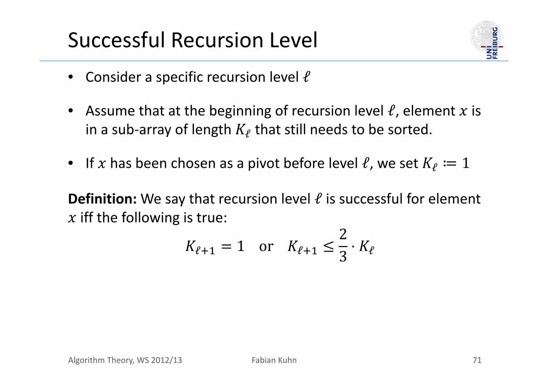
Successful Recursion Level• Consider a specific recursion level ℓ

• Assume that at the beginning of recursion level ℓ, element is in a sub‐array of length ℓ that still needs to be sorted.

• If has been chosen as a pivot before level ℓ, we set ℓ ≔ 1

Definition: We say that recursion level ℓ is successful for element iff the following is true:

ℓ 1or ℓ23 ⋅ ℓ


Successful Recursion LevelLemma: For every recursion level ℓ and every array element , it holds that level ℓ is successful for with probability at least ⁄ , independently of what happens in other recursion levels.

Proof:


Number of Successful Recursion LevelsLemma: If among the first ℓ recursion levels, at least log ⁄are successful for element , we have ℓ 1.

Proof:


Number of Comparisons for Lemma: For every array element , with high probability, as a non‐pivot, is compared to a pivot at most log times.

Proof:


Number of ComparisonsTheorem: With high probability, the total number of comparisons is at most .

Proof:

Algorithm Theory WS Fabian Kuhn - ac.informatik.uni...

Documents

Transcript of Algorithm Theory WS Fabian Kuhn - ac.informatik.uni...