Algorithm Theoretical Basis Document (ATBD) · PDF fileconstituents or to provide the inherent...

GKSS Research Centre GeesthachtInstitute for Coastal Research

MERIS

Regional Case II Water Algorithm

Atmospheric Correction ATBD

DOC: GKSS-KOF-MERIS-ATBD01Name: MERIS Case II ATBD-ATMOIssue: 1.0 Rev: 0.0Date: 8. June 2008Page: 1

Algorithm Theoretical Basis Document (ATBD)

MERIS Regional Coastal and Lake Case 2 Water Project


Version 1.0, 18. May 2008

Roland Doerffer & Helmut Schiller

GKSS Forschungszentrum Geesthacht GmbH

21502 Geesthacht

ESRIN Contract: No. 18639/04/I-LG

MERIS Case 2 Water Algorithms Development

&

Development of MERIS lake water algorithms

ESRIN Contract No. 20436/06/I-LG

Copyright ©2008 GKSS GmbH


MERIS




Distribution

Name:

P. Regner (ESA / ESRIN)

S. Koponen

C. Brockmann (BC)

Change Record

Issue Revision Date DescriptionVersion 1.0 0.0 8. June 2008



MERIS




Table of Content1 Overview........................................................................................................................................................42 Preface..........................................................................................................................................................63 ATBD History.................................................................................................................................................64 Introduction....................................................................................................................................................65 Algorithm Overview........................................................................................................................................76 Theoretical Description................................................................................................................................11

6.1 Optical Components of the Atmosphere..............................................................................................116.1.1 Aerosols.......................................................................................................................................116.1.2 Cirrus...........................................................................................................................................166.1.3 Specular reflection at the sea surface..........................................................................................176.1.4 Water leaving radiance................................................................................................................18

6.2 Vertical distribution and concentration ranges....................................................................................186.2.1 Rayleigh scattering.......................................................................................................................196.2.2 Ozone absorption.........................................................................................................................196.2.3 Aerosols and Cirrus.....................................................................................................................20

7 Radiative transfer modelling.........................................................................................................................267.1 Computation of the upward directed radiance transmittances..............................................................287.2 Wavelengths used for simulations.......................................................................................................30

8 Training of the neural network......................................................................................................................308.1 The training of the atmospheric correction NN....................................................................................338.2 The performance of the NN................................................................................................................33

9 Implementation of the atmospheric correction procedure in BEAM..............................................................369.1 Computation of RL_tosa from RL_toa..................................................................................................37

9.1.1 Correction for ozone....................................................................................................................379.1.2 Correction for Rayleigh scattering...............................................................................................37

9.2 Correction of water vapour influence on MERIS band 9 708 nm..........................................................389.3 Use of cartesian coordinates................................................................................................................399.4 Computation of the angstrom coefficient..............................................................................................409.5 Correction of camera boundary problem (“smile effect”)......................................................................40

10 References................................................................................................................................................41



MERIS




1 OverviewThis document describes a procedure for the atmospheric correction of radiance spectra measured with the Medium Resolution Imaging Spectrometer (MERIS) over turbid case II coastal and inland waters. MERIS is part of the European Environmental Satellite ENVISAT as one of ten instruments and is operated by the European Space Agency ESA.

For the evaluation of its data products by users the software package BEAM has been developed by Brockmann Consult on behalf of ESA. This package mainly allows the display and the analysis of the standard data products of level 1 and level 2 provided by ESA. However, these standard products do not provide optimal results for all areas. In particular case 2 water areas, mainly coastal and inland waters, may require adapted algorithms to retrieve the concentrations of water constituents or to provide the inherent optical properties. In particular the case 2 water atmospheric correction procedure, as implemented in the standard MERIS ground segment, may not be optimum in special cases. In particular in turbid waters it produces negative reflectances in the blue bands, or, in case 1 waters, in the red bands. In order to enable users to derive products also for those special or regional cases, where the standard processor is not sufficient, a processor has been developed in form of a plug-in for BEAM, which consists of a procedure for atmospheric correction and procedures for determining inherent optical properties and concentrations of water constituents for coastal and different lake waters.

This ATBD describes the atmospheric correction procedure of this plug-in.

The Atmospheric Correction is defined here as the determination of the water leaving radiance reflectance spectrum (RLw(λ)) from the top-of-atmosphere radiance reflectance spectrum (RL_toa(λ)). It requires the determination of the radiance backscattered from all targets above the water surface including air molecules, aerosols, thin clouds, foam on the water as well as all radiance which is specularly reflected at the water surface, in particular the sun glint. Furthermore, the transmission of the solar radiance through the atmosphere to the water surface and of the radiance from the water surface to the sensor has to be computed.

The atmospheric correction procedure is based on radiative transfer simulations. The simulated radiance reflectances are used to train a neural network, which, in turn, is used for the parametrization of the relationship between the top of atmosphere radiance reflectances, RL_toa and the water leaving radiance reflectances (RLw). Furthermore it computes (1) the atmospheric path radiances (RL_path), (2) the downwelling irradiance at water level (Ed), (3) the aerosol optical thickness at 550 nm and three other wavelengths and (4) the angstrom exponents of the aerosol optical thickness. The water leaving radiance reflectances (RLw) of the first 9 MERIS bands are then input to another procedure for retrieving the IOPs and concentrations of the water constituents (s. corresponding ATBD for water constituents of coastal and inland waters).

The model atmosphere comprises three parts: (1) a standard atmosphere, which includes 50 layers with variable concentrations of different aerosols, cirrus cloud particles and a rough, wind dependent sea surface with specular reflectance, but with a constant air pressure- and ozone



MERIS




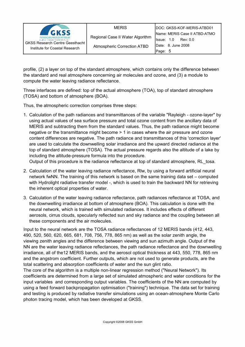
profile, (2) a layer on top of the standard atmosphere, which contains only the difference between the standard and real atmosphere concerning air molecules and ozone, and (3) a module to compute the water leaving radiance reflectance.

Three interfaces are defined: top of the actual atmosphere (TOA), top of standard atmosphere (TOSA) and bottom of atmosphere (BOA).

Thus, the atmospheric correction comprises three steps:

1. Calculation of the path radiances and transmittances of the variable "Rayleigh - ozone-layer" by using actual values of sea surface pressure and total ozone content from the ancillary data of MERIS and subtracting them from the standard values. Thus, the path radiance might become negative or the transmittance might become > 1 in cases where the air pressure and ozone content differences are negative. The path radiance and transmittances of this 'correction layer' are used to calculate the downwelling solar irradiance and the upward directed radiance at the top of standard atmosphere (TOSA). The actual pressure regards also the altitude of a lake by including the altitude-pressure formula into the procedure.Output of this procedure is the radiance reflectance at top of standard atmosphere, RL_tosa.

2. Calculation of the water leaving radiance reflectance, Rlw, by using a forward artificial neural network fwNN. The training of this network is based on the same training data set – computed with Hydrolight radiative transfer model -, which is used to train the backward NN for retrieving the inherent optical properties of water.

3. Calculation of the water leaving radiance reflectance, path radiances reflectance at TOSA, and the downwelling irradiance at bottom of atmosphere (BOA). This calculation is done with the neural network, which is trained with simulated radiances. It includes effects of different aerosols, cirrus clouds, specularly reflected sun and sky radiance and the coupling between all these components and the air molecules.

Input to the neural network are the TOSA radiance reflectances of 12 MERIS bands (412, 443, 490, 520, 560, 620, 665, 681, 708, 756, 778, 865 nm) as well as the solar zenith angle, the viewing zenith angles and the difference between viewing and sun azimuth angle. Output of the NN are the water leaving radiance reflectances, the path radiance reflectance and the downwelling irradiance, all of the12 MERIS bands, and the aerosol optical thickness at 443, 550, 778, 865 nm and the angstrom coefficient. Further outputs, which are not used to generate products, are the total scattering and absorption coefficients of water and the sun glint ratio.The core of the algorithm is a multiple non-linear regression method ("Neural Network"). Its coefficients are determined from a large set of simulated atmospheric and water conditions for the input variables and corresponding output variables. The coefficients of the NN are computed by using a feed forward backpropagation optimisation ("training") technique. The data set for training and testing is produced by radiative transfer simulations using an ocean-atmosphere Monte Carlo photon tracing model, which has been developed at GKSS.



MERIS




2 PrefaceOne instrument of the ENVISAT earth observation mission of the European Space Agency ESA is the Medium Resolution Imaging Spectrometer MERIS. This instrument is used to measure properties of the atmosphere and land surfaces and the ocean. Prime mission is the determination of optical properties of oceanic water and the concentrations of its constituents. For open ocean water robust methods have been developed for the correction of the atmospheric influence as well as the retrieval of phytoplankton chlorophyll. This is not so the case for some types of coastal waters as well as inland waters, where the case 1 water routines for the atmospheric correction and the retrieval of water constituents fail. Also the standard extension of the atmospheric correction to turbid coastal waters fail in some areas so that the case 2 water algorithm for the retrieval cannot be applied. These areas have to be flagged and thus are lost for further use.

This ATBD describes the atmospheric correction procedure, which is used to calculate water leaving radiance reflectances from top of atmosphere radiances. One requirement for this procedure is to include turbid case 2 waters into the scope of the algorithm. The standard MERIS atmospheric correction procedure for case II water, as implemented in the ground segment, is adapted to waters with only limited concentrations of suspended solids and yellow substances and leads under other cases to negative reflectances and artefacts. Thus, it was necessary to write a new procedure for BEAM. This opportunity was used to develop and test a new type of atmospheric correction method which is based on inverse modelling and its parametrization by a neural network. It takes into account the effect of cirrus clouds, specularly reflected sun light (sun glint) and the water leaving radiance reflectances caused by all sort of water constituents.

3 ATBD HistoryThe procedure described in this document is the first version. It is partly based on principles and results, which have been developed for the MOS sensor and a previous version of an atmospheric correction procedure for MERIS.

4 IntroductionRemote sensing of water constituents require a careful atmospheric correction since more than 90% of the upward directed radiance at satellite altitude stems from the atmosphere including direct sunlight and skylight, which are specularly reflected at the sea surface. Small errors in determining the optical properties of the atmospheric may induce large errors in the retrieval of water constituent concentrations.

During the era of the Coastal Zone Colour Scanner (CZCS) atmospheric correction schemes have been developed for open ocean case I water, which were based on the following assumptions:

• the atmospheric path radiance can be split in a molecular scattering component (Rayleigh scattering) and an aerosol scattering component,

• the water leaving radiance in the near infrared spectral bands is neglectably small (due to high



MERIS




water absorption) so that the radiance at top of atmosphere, after subtracting the contribution by molecular scattering, is only influenced by aerosols,

• the spectral extinction of aerosols can be described by an exponential function, which allows an extrapolation from the near infrared to the blue-green spectral range.

Different versions of this procedure have been discussed in various papers; their underlying principles are summarised in an overview by Gordon and Morel (1983).

However, the new generation of ocean colour sensors requires a more sophisticated procedure in order to utilise the higher radiometric accuracy of these sensors for the retrieval of water substances. In particular the assumptions that (1) the spectral distribution of the extinction can be described by a single number, i.e. the Angstrom exponent, and (2) the atmosphere can be separated into a Rayleigh- and an aerosol layer, lead to errors, which are not acceptable with respect to the increased sensor accuracy as present in MERIS.

Thus, the new atmospheric correction procedures for case I water such as developed for SeaWiFS, MODIS and MERIS include the aerosol-Rayleigh coupling as well as a detailed description of the spectral variability of different aerosol types (s. Antoine and Morel, 1998) and the ATBD for case I water atmospheric correction of MERIS.

Three problems are not or not sufficiently solved so far for the operational atmospheric correction of ocean colour data: (1) atmospheric correction over turbid water, where also the near infrared spectral bands are influenced by scattering of suspended particles, (2) the scattering by thin or subvisible cirrus clouds including aged jet trails and (3) specularly reflected sun light, which is present even in the nadir radiances, and, of course, a combination of these problems.

All of these factors are included in the correction procedure as described in this ATBD.

5 Algorithm OverviewIn conventional atmospheric correction procedures two properties have to be determined from the radiance or reflectances in the near infrared spectral range: (1) the Angstrom exponent, which assumes and describes an exponential spectral shape of the path radiance spectrum of aerosols, and which has to be determined from at least two of the NIR bands, and (2) the path radiance in one of the near infrared bands. The path radiances in the blue-green spectral bands are then calculated by extrapolation using the exponent and radiance of one of the NIR bands.

However, this method cannot be applied to case II waters with high suspended matter concentrations, where the backscattering of water cannot be neglected in the NIR bands. The problem can be solved by inverse modelling of the radiative transfer, where the concentrations of water constituents as well as of aerosols are modified and, thus, determined with the help of an optimization procedure, which is used to minimize the deviation between the measured and the modelled radiance spectra. This approach was applied to CZCS images, where only four spectral channels were available for retrieving water constituents and aerosols (Doerffer & Fischer, 1993).



MERIS




Due to the lack of near infrared bands, it was only possible to retrieve the aerosol path radiance by assuming a constant aerosol type (Angstrom exponent) for the entire image.

Another major problem is the influence of thin cirrus clouds including aged jet trails, which may sustain for hours under humid conditions. These thin cirrus causes most of the problems particularly in the retrieval of phytoplankton pigment and yellow substance in coastal areas with heavy air traffic. Furthermore, even with a simple model, such as used for the CZCS data, the inversion method requires an amount of computational time which is not acceptable for the mass processing of satellite scenes.

To combine a realistic description of the processes in the atmosphere using a detailed radiative transfer model with the required high computational efficiency, a neural network procedure was developed.

The NN technique was first tested for the atmospheric correction of MERIS data (Schiller & Doerffer, 1999) using the concentrations of three substances and one aerosol as independent variables. However, also this approach did not consider different aerosol types or an Angstrom coefficient as an independent variable. Thus, we have designed a new scheme with different alternatives.

Common to all developed procedures in the course of this project is the model of the atmosphere, different is the way of how the contribution by the water leaving radiance is handled. Three alternatives have been investigated:

1. The water leaving radiance reflectance is only computed for the 4 near infrared bands at 708, 753, 779 and 865 nm, for all other bands in the blue to green range the tosa radiance reflectance is simulated for a black ocean. The NN is trained to determine the path radiance reflectance and the downwelling irradiance at bottom of atmosphere (BOA). The water leaving radiance reflectance is then computed from the path radiance and transmittance also for the green-blue bands.

2. An additional band at 412 or 560 nm is included with the idea of reducing the extrapolation problem.

3. The water leaving radiance reflectance is simulated for all bands. The NN is trained that it determines the Rlws directly from the corresponding RL_tosa values.

Disadvantage of the third alternative is that a full bio-optical model for the water has to be included, so that the procedure is not independent from the water model. However, the big advantage is that the extrapolation from the NIR bands is avoided and that by definition no negative reflectances can occur. All three alternative have been tested for various cases. As it turned out procedure 3, which includes the RLws of all bands, has the best results and was selected finally as the atmospheric correction scheme. Thus, in the following we will only describe details of this third procedure, which is characterized by the following features:



MERIS




• The forward model is a Monte Carlo photon tracing model, which describes in a realistic way the radiative transfer within the ocean-atmosphere system. It consists of an atmosphere with 50 layers, a rough sea surface and a homogeneous water body below. However, the water part was not used: because of the high optical thickness of water, photon tracing requires too much computational time for mass radiance spectra calculations. Instead the water leaving radiance was computed with the forward NN, which is trained with spectra computed with the Hydrolight model. Within the atmosphere the concentrations of aerosols and cirrus particles vary within a defined range, while the density profile of air molecules and ozone is kept constant.

• A large range of different aerosols with different optical properties and a realistic vertical distribution is used in the forward calculations.

• Scattering by thin cirrus clouds at top of the troposphere has been included.

• The water leaving radiance of the water body is computed using a forward NN, which is trained with simulated directional water leaving radiances and the corresponding water optical properties, i.e. for coastal water the C2R bio-optical model was used and for the Boreal lakes the Boreal bio-optical model.

• Specularly reflected direct sun radiation (sun glint) and sky radiation (skylight glint) is taken into account for the full swath of MERIS and for various wind speeds.

Since the vertical profile for Rayleigh scattering and ozone absorption was kept constant for the training of the NN - in order to keep the number of variables as small as possible - , it was necessary to compute the deviations from the fixed profile with respect to ozone absorption and Rayleigh scattering in a separate procedure before using the NN. Thus, a top of standard atmosphere (TOSA) was defined for which the radiance reflectance spectrum RL_tosa has to be calculated from the top of atmosphere radiance reflectance RL_toa by knowing the deviation of the air pressure and ozone concentration from that of the standard atmosphere (i.e. 1013.2 hPa for pressure and 350 DU for ozone).



MERIS




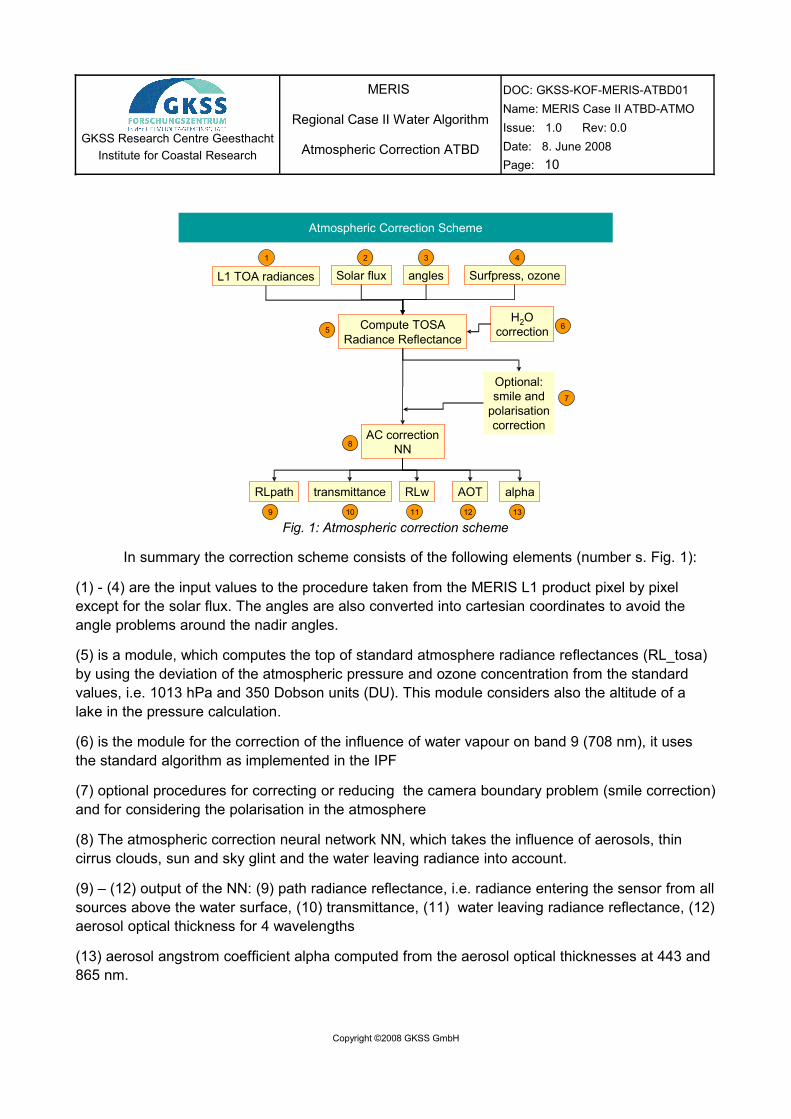
Fig. 1: Atmospheric correction scheme

In summary the correction scheme consists of the following elements (number s. Fig. 1):

(1) - (4) are the input values to the procedure taken from the MERIS L1 product pixel by pixel except for the solar flux. The angles are also converted into cartesian coordinates to avoid the angle problems around the nadir angles.

(5) is a module, which computes the top of standard atmosphere radiance reflectances (RL_tosa) by using the deviation of the atmospheric pressure and ozone concentration from the standard values, i.e. 1013 hPa and 350 Dobson units (DU). This module considers also the altitude of a lake in the pressure calculation.

(6) is the module for the correction of the influence of water vapour on band 9 (708 nm), it uses the standard algorithm as implemented in the IPF

(7) optional procedures for correcting or reducing the camera boundary problem (smile correction) and for considering the polarisation in the atmosphere

(8) The atmospheric correction neural network NN, which takes the influence of aerosols, thin cirrus clouds, sun and sky glint and the water leaving radiance into account.

(9) – (12) output of the NN: (9) path radiance reflectance, i.e. radiance entering the sensor from all sources above the water surface, (10) transmittance, (11) water leaving radiance reflectance, (12) aerosol optical thickness for 4 wavelengths

(13) aerosol angstrom coefficient alpha computed from the aerosol optical thicknesses at 443 and 865 nm.


Atmospheric Correction Scheme

L1 TOA radiances Solar flux angles Surfpress, ozone

Compute TOSARadiance Reflectance

Optional:smile and

polarisationcorrection

AC correctionNN

RLpath RLwtransmittance AOT alpha

H2Ocorrection

1 2 3 4

5 6

7

8

9 10 11 12 13


MERIS




6 Theoretical Description6.1 Optical Components of the Atmosphere

Task of the atmospheric correction in the processing of ocean colour satellite data is the retrieval of the water leaving radiance, which contains information about the optical properties of the water and it constituents. All other contributions to the radiance at top of atmosphere have to be determined and subtracted. This includes the atmospheric path radiance caused by scattering at air molecules, aerosols and thin clouds and the sun skylight specularly reflected at the water surface or reflected at foam and other surface material. Finally the transmittance of the water leaving radiance through the atmosphere has to be computed.

A coastal atmosphere may contain different kinds of aerosols with different optical properties and with a rapidly changing distribution in time and space. The mean aerosol climate depends on the area (industrial coast, volcanoes, deserts, air traffic with jet trails) and the main wind direction. However, the actual aerosol composition and the vertical distribution above a pixel cannot be determined from climatological data but only from observations at the time of overflight. Thus, for atmospheric correction of satellite images, it is important to derive the optical properties of the atmosphere from the radiance measurements of the sensor itself.

Because of the complicated mixture of different aerosols and its vertical distribution, and the limited number of independent spectral information, it is necessary to reduce the complexity of all variables to a small number of components, which describe the optical variability. Since for atmospheric correction it is not the task to identify different aerosols, it is sufficient to correct for its impact on the top of atmosphere radiances.

MERIS has 4 spectral bands which are used for atmospheric correction in the procedure described here (708, 753, 778 and 865 nm ). An important assumption is that the toa-radiances at these four bands are sufficient to describe the spectral radiance variability caused by aerosols, cirrus clouds, sun glint and suspended particles. However, since the use of only these 4 bands requires an extrapolation into the green-blue spectral range, which can cause problems in particular over waters with high concentrations of absorbing and/or scattering constituents, it was decided to use in addition also the blue-green bands, i.e. all together 12 MERIS bands to perform the atmospheric correction.

In the next sections we will describe all components of the system in detail.

6.1.1 AerosolsThe properties of the aerosols, which are used in the simulations and which define the scope of the algorithm, are adopted from WCRP 112 (1986), Shettle & Fenn (1979), from the MERIS atmospheric correction ATBD (Antoine & Morel, 1999) and from the Mie program of the Institute for Space Science, FUB Berlin (Heinemann & Schüller, 1995).

According to the recommendations of WCRP112, aerosols are constructed from basic aerosol



MERIS




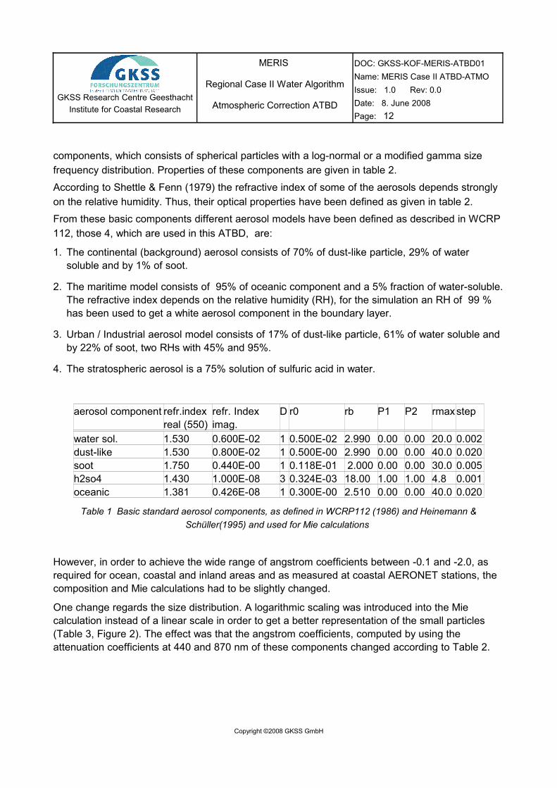
components, which consists of spherical particles with a log-normal or a modified gamma size frequency distribution. Properties of these components are given in table 2.

According to Shettle & Fenn (1979) the refractive index of some of the aerosols depends strongly on the relative humidity. Thus, their optical properties have been defined as given in table 2.

From these basic components different aerosol models have been defined as described in WCRP 112, those 4, which are used in this ATBD, are:

1. The continental (background) aerosol consists of 70% of dust-like particle, 29% of water soluble and by 1% of soot.

2. The maritime model consists of 95% of oceanic component and a 5% fraction of water-soluble. The refractive index depends on the relative humidity (RH), for the simulation an RH of 99 % has been used to get a white aerosol component in the boundary layer.

3. Urban / Industrial aerosol model consists of 17% of dust-like particle, 61% of water soluble and by 22% of soot, two RHs with 45% and 95%.

4. The stratospheric aerosol is a 75% solution of sulfuric acid in water.

aerosol component refr.index real (550)

refr. Index imag.

D r0 rb P1 P2 rmaxstep

water sol. 1.530 0.600E-02 1 0.500E-02 2.990 0.00 0.00 20.0 0.002dust-like 1.530 0.800E-02 1 0.500E-00 2.990 0.00 0.00 40.0 0.020soot 1.750 0.440E-00 1 0.118E-01 2.000 0.00 0.00 30.0 0.005h2so4 1.430 1.000E-08 3 0.324E-03 18.00 1.00 1.00 4.8 0.001oceanic 1.381 0.426E-08 1 0.300E-00 2.510 0.00 0.00 40.0 0.020

Table 1 Basic standard aerosol components, as defined in WCRP112 (1986) and Heinemann & Schüller(1995) and used for Mie calculations

However, in order to achieve the wide range of angstrom coefficients between -0.1 and -2.0, as required for ocean, coastal and inland areas and as measured at coastal AERONET stations, the composition and Mie calculations had to be slightly changed.

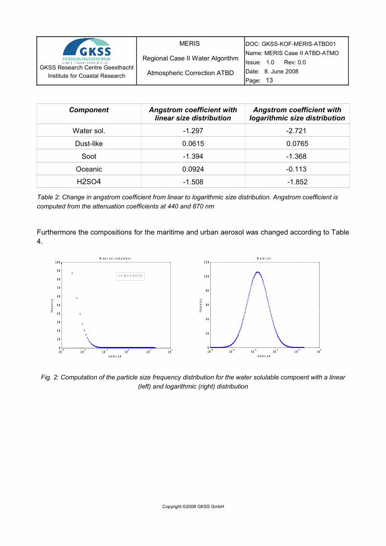
One change regards the size distribution. A logarithmic scaling was introduced into the Mie calculation instead of a linear scale in order to get a better representation of the small particles (Table 3, Figure 2). The effect was that the angstrom coefficients, computed by using the attenuation coefficients at 440 and 870 nm of these components changed according to Table 2.



MERIS




Component Angstrom coefficient with linear size distribution

Angstrom coefficient with logarithmic size distribution

Water sol. -1.297 -2.721

Dust-like 0.0615 0.0765

Soot -1.394 -1.368

Oceanic 0.0924 -0.113

H2SO4 -1.508 -1.852

Table 2: Change in angstrom coefficient from linear to logarithmic size distribution. Angstrom coefficient is computed from the attenuation coefficients at 440 and 870 nm

Furthermore the compositions for the maritime and urban aerosol was changed according to Table 4.


Fig. 2: Computation of the particle size frequency distribution for the water solulable compoent with a linear (left) and logarithmic (right) distribution

1 0- 3

1 0- 2

1 0- 1

1 00

1 01

1 02

0

1 0

2 0

3 0

4 0

5 0

6 0

7 0

8 0

9 0

1 0 0

r a d i u s µ m

freq

uenc

y

W a t e r s o l . c o m p o n e n t

r = 0 . 0 0 1 : 0 . 0 0 2 : 2 0

1 0- 3

1 0- 2

1 0- 1

1 00

1 01

1 02

0

1 0

2 0

3 0

4 0

5 0

6 0

7 0

8 0

9 0

1 0 0

1 0- 3

1 0- 2

1 0- 1

1 00

1 01

1 02

0

1 0

2 0

3 0

4 0

5 0

6 0

7 0

8 0

9 0

1 0 0

r a d i u s µ m

freq

uenc

y

W a t e r s o l . c o m p o n e n t

r = 0 . 0 0 1 : 0 . 0 0 2 : 2 0

1 0- 5

1 0- 4

1 0- 3

1 0- 2

1 0- 1

1 00

0

2 0

4 0

6 0

8 0

1 0 0

1 2 0

r a d i u s µ m

freq

uenc

y

W a t e r s o l .

1 0- 5

1 0- 4

1 0- 3

1 0- 2

1 0- 1

1 00

0

2 0

4 0

6 0

8 0

1 0 0

1 2 0

1 0- 5

1 0- 4

1 0- 3

1 0- 2

1 0- 1

1 00

0

2 0

4 0

6 0

8 0

1 0 0

1 2 0

r a d i u s µ m

freq

uenc

y

W a t e r s o l .


MERIS




output-file: mwang1c.sex (09) mqco = optical properties

mwamg1c.pfu (10) mpco = phase-function

No. name(10char) wavel. RFR RFI Typ r0 rb P3 P4 rmax nstep rmin

101 water sol. 0.5500 1.530 0.600E-02 1 0.500E-02 2.990 0.00 0.00 0.2 500 0.00001

102 dust-like 0.5500 1.530 0.800E-02 1 0.500E-00 2.990 0.00 0.00 10.0 500 0.00200

103 soot 0.5500 1.750 0.440E-00 1 0.118E-01 2.000 0.00 0.00 0.2 500 0.00050

104 oceanic 0.5500 1.381 0.426E-08 1 0.300E-00 2.510 0.00 0.00 5.0 500 0.00200

106 rural99 0.5500 1.000 0.111E-00 1 5.215E-02 2.239 0.00 0.00 1.0 500 0.00050

107 urban50 0.5500 1.000 0.111E-00 1 2.563E-02 2.239 0.00 0.00 1.0 500 0.00050

190 h2so4 0.5500 1.430 1.000E-08 3 0.324E-03 18.00 1.00 1.00 2.0 500 0.00005

0 ENDE 0.0000 0.000 0.000E+00 0 0.000E-00 0.000 0.00 0.00 0.0 000 0.00000

4 Spektrum

meris_lam_nomi_20051023.txt

101 rfi/watsol.rfi

102 rfi/dust.rfi

103 rfi/soot.rfi

104 rfi/oceanic.rfi

106 rfi/sflr99.rfi

107 rfi/sfsu50.rfi

190 rfi/h2so4.rfi

123456789-123456789-123456789-123456789-123456789-123456789-123456789-123456789

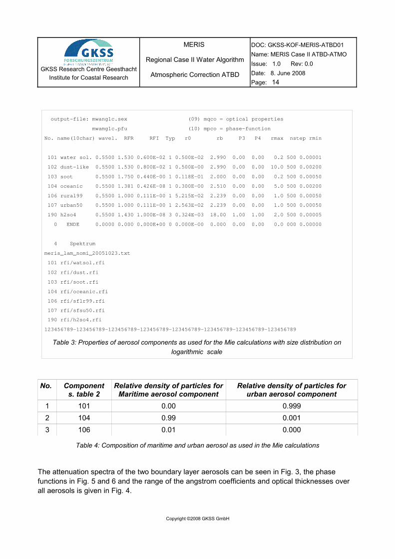
Table 3: Properties of aerosol components as used for the Mie calculations with size distribution on logarithmic scale

No. Components. table 2

Relative density of particles for Maritime aerosol component

Relative density of particles for urban aerosol component

1 101 0.00 0.9992 104 0.99 0.0013 106 0.01 0.000

Table 4: Composition of maritime and urban aerosol as used in the Mie calculations

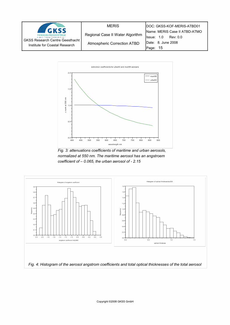
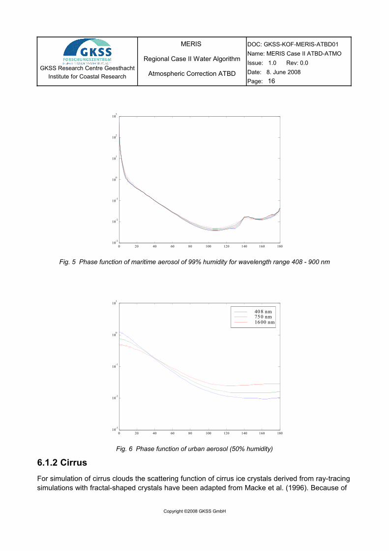
The attenuation spectra of the two boundary layer aerosols can be seen in Fig. 3, the phase functions in Fig. 5 and 6 and the range of the angstrom coefficients and optical thicknesses over all aerosols is given in Fig. 4.



MERIS




Fig. 3: attenuations coefficients of maritime and urban aerosols, normalized at 550 nm. The maritime aerosol has an angstroem coefficient of – 0.065, the urban aerosol of - 2.15

Fig. 4: Histogram of the aerosol angstrom coefficients and total optical thicknesses of the total aerosol


400 450 500 550 600 650 700 750 800 850 9000.0

0.5

1.0

1.5

2.0

extinction coefficients for u rba50 and m ari99 aeroso ls

waveleng th nm

c no

rm a

t 550

nm

m ari99

urba50

-2.2 -2 .0 -1 .8 -1 .6 -1 .4 -1 .2 -1 .0 -0 .8 -0 .6 -0 .4 -0.2 0.00.0

0.1

0.2

0.3

0.4

0.5

0.6

0.7

0.8

0.9

Histogram of angstrom coefficien t

angstrom coefficien t 442/865

frequ

ency

0.0 0.5 1.0 1.50.0

0.2

0.4

0.6

0.8

1.0

1.2

1.4

1.6

1.8

Histogram of optical thickness tau550

optical thickness

frequ

ency


MERIS




Fig. 5 Phase function of maritime aerosol of 99% humidity for wavelength range 408 - 900 nm

Fig. 6 Phase function of urban aerosol (50% humidity)

6.1.2 CirrusFor simulation of cirrus clouds the scattering function of cirrus ice crystals derived from ray-tracing simulations with fractal-shaped crystals have been adapted from Macke et al. (1996). Because of


0 20 40 60 80 100 120 140 160 18010-3

10-2

10-1

100

101

102

103

angle [deg]

()/b [s r

-1]

0 20 40 60 80 100 120 140 160 18010-3

10-2

10-1

100

101

angle [deg]

()/b [s r

-1]

40 8 nm75 0 nm16 00 nm


MERIS




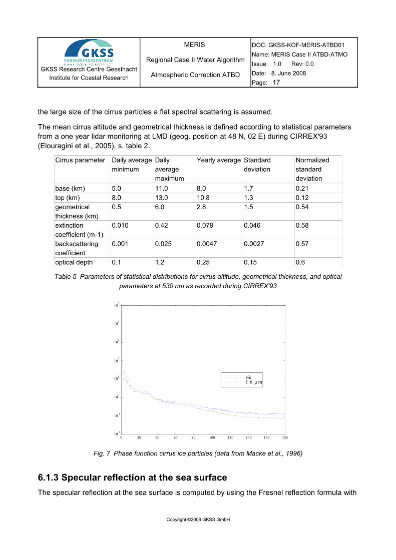
the large size of the cirrus particles a flat spectral scattering is assumed.

The mean cirrus altitude and geometrical thickness is defined according to statistical parameters from a one year lidar monitoring at LMD (geog. position at 48 N, 02 E) during CIRREX'93 (Elouragini et al., 2005), s. table 2.

Cirrus parameter Daily average minimum

Daily average maximum

Yearly average Standard deviation

Normalized standard deviation

base (km) 5.0 11.0 8.0 1.7 0.21top (km) 8.0 13.0 10.8 1.3 0.12geometrical thickness (km)

0.5 6.0 2.8 1.5 0.54

extinction coefficient (m-1)

0.010 0.42 0.079 0.046 0.58

backscattering coefficient

0.001 0.025 0.0047 0.0027 0.57

optical depth 0.1 1.2 0.25 0.15 0.6

Table 5 Parameters of statistical distributions for cirrus altitude, geometrical thickness, and optical parameters at 530 nm as recorded during CIRREX'93

Fig. 7 Phase function cirrus ice particles (data from Macke et al., 1996)

6.1.3 Specular reflection at the sea surfaceThe specular reflection at the sea surface is computed by using the Fresnel reflection formula with


0 20 40 60 80 100 120 140 160 18010-2

10-1

100

101

102

103

104

105

angle [deg]

()/b [s r

-1]

vis1.6 µ m


MERIS




the refractive index of sea water of 1.34 for all bands. The surface slopes of the waves are computed as a function of the wind speed using the formulation of Cox&Munk (1954).

6.1.4 Water leaving radianceThe water leaving radiance is computed by using a forward neural network. For coastal water the NN 55x20_2295.4.net has been used. Its input are

● the scattering coefficient for all particles, range b(442 nm) 0.01 – 59.5 m-1,

● the absorption of phytoplankton pigments, range a(442 nm) 0.001 – 2.0 m-1, and

● the absorption of yellow substance and bleached particles, range a(442 nm) 0.0029 – 9.2 m-1.

Output are the water leaving radiances at 12 MERIS bands. For the Boreal lake and the Eutrophic Lake processors different NNs has been used, which are based on the corresponding bio-optical models of the two types of lakes. Details are described in the corresponding ATBDs for the retrieval of water constituents.

6.2 Vertical distribution and concentration ranges

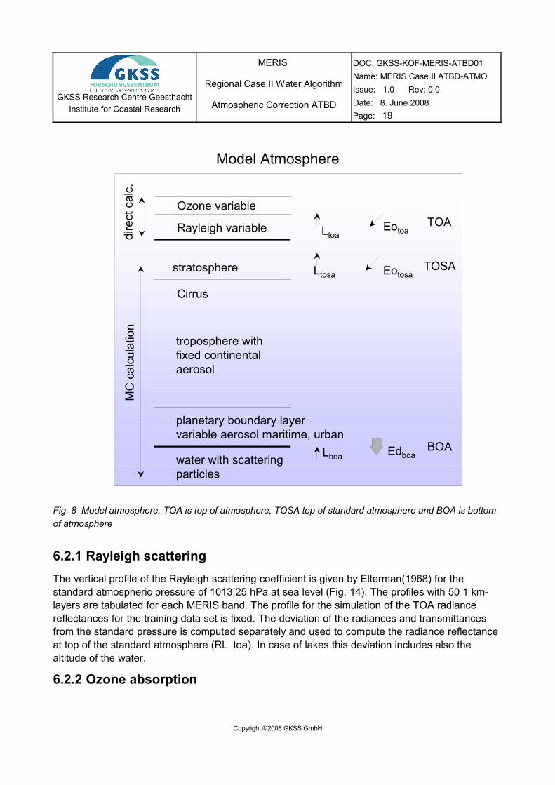
The atmosphere model (Fig. 8) is separated in two parts: Part 1 contains the variable aerosol / cirrus concentrations with a constant Rayleigh scattering and ozone absorption profile. It has 50 layers, each 1 km thick. Part 2 consists of 2 virtual layers on top of this standard atmosphere with only a variable ozone and Rayleigh scattering atmosphere. These two second layers are used to correct for the deviations of these two quantities from the standard profile of part 1, where they are constant. They may get negative radiances or transmittances > 1. The deviations are computed as the difference between the standard values and the ozone content and surface pressure are taken from the MERIS standard L1 product (s. chapter 9.1).



MERIS




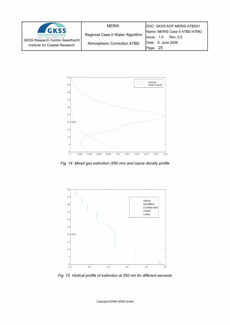
6.2.1 Rayleigh scatteringThe vertical profile of the Rayleigh scattering coefficient is given by Elterman(1968) for the standard atmospheric pressure of 1013.25 hPa at sea level (Fig. 14). The profiles with 50 1 km-layers are tabulated for each MERIS band. The profile for the simulation of the TOA radiance reflectances for the training data set is fixed. The deviation of the radiances and transmittances from the standard pressure is computed separately and used to compute the radiance reflectance at top of the standard atmosphere (RL_toa). In case of lakes this deviation includes also the altitude of the water.

6.2.2 Ozone absorption


Fig. 8 Model atmosphere, TOA is top of atmosphere, TOSA top of standard atmosphere and BOA is bottom of atmosphere

Model Atmosphere

TOAOzone variable

Rayleigh variable

Cirrus

troposphere withfixed continentalaerosol

planetary boundary layervariable aerosol maritime, urban

TOSA

BOAwater with scatteringparticles

Ltosa

Ltoa

Lboa

Eotoa

Eotosa

Edboa

MC

cal

cula

tion

dire

ct c

alc.

stratosphere


MERIS




The vertical ozone profile is taken from Elterman(1968), Fig. 14. The density profile is given in cm ozone per km for a surface pressure of 1013.25 hP. The total ozone column content is 0.35 cm. The extinction profiles with 50 1-km-layers are tabulated for each MERIS band. Also the ozone profile is fixed for the simulation of the training data set. Deviations from the standard concentration of 350 Dobson units (DU) are computed in a separate module (s. chapter 9.11).

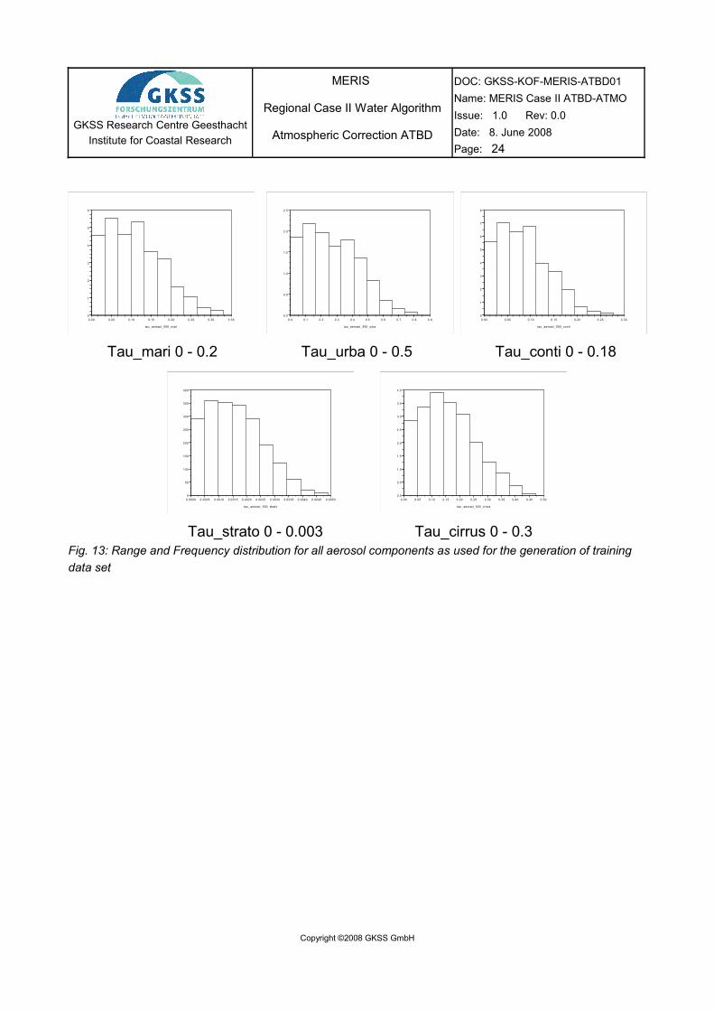
6.2.3 Aerosols and CirrusEach of the 4 aerosol and cirrus has a predefined vertical profile within the model atmosphere of 50 layers with maximum concentrations for each layer (Fig. 15, Table 6). During the simulation run the concentration profile for each aerosol / cirrus component is modified by a randomly selected factor in the range 0 and 1. In the extreme minimum case the whole atmosphere consists only of Rayleigh scattering and ozone absorption.

The aerosol / cirrus optical thicknesses for this model atmosphere are given in table 6 and the profiles of the maximum values are given in Fig.15

As one can see from this table, the dominating effects come from the urban aerosol, the maritime aerosol and the cirrus clouds.

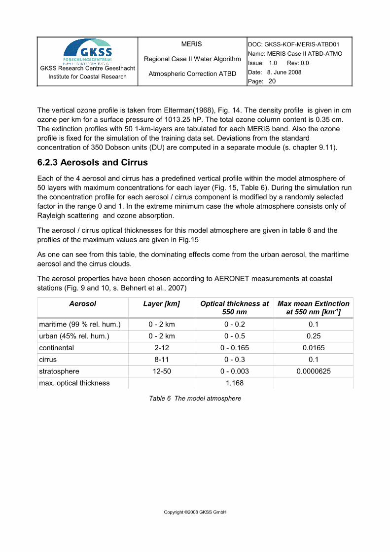
The aerosol properties have been chosen according to AERONET measurements at coastal stations (Fig. 9 and 10, s. Behnert et al., 2007)

Aerosol Layer [km] Optical thickness at 550 nm

Max mean Extinction at 550 nm [km-1]

maritime (99 % rel. hum.) 0 - 2 km 0 - 0.2 0.1urban (45% rel. hum.) 0 - 2 km 0 - 0.5 0.25continental 2-12 0 - 0.165 0.0165cirrus 8-11 0 - 0.3 0.1stratosphere 12-50 0 - 0.003 0.0000625max. optical thickness 1.168

Table 6 The model atmosphere



MERIS





Fig. 9: Aerosol optical thickness determined at coastal and oceanic AERONET stations for 200-2003 (Behnert et al., 2007)


MERIS




One problem was to create a uniform distribution over the full range of optical properties of aerosols during the simulation runs. If each of the aerosol components is randomly selected from a uniform distribution over its range 0 – max then the overall frequency distribution of the total attenuation coefficients (sum of the attenuation of all aerosol/cirrus components) becomes a Gaussian distribution. The consequence for the training of the neural network is a bias around the mean of the distribution. Thus, another distribution for the random selection of the concentration of each component has to be created.

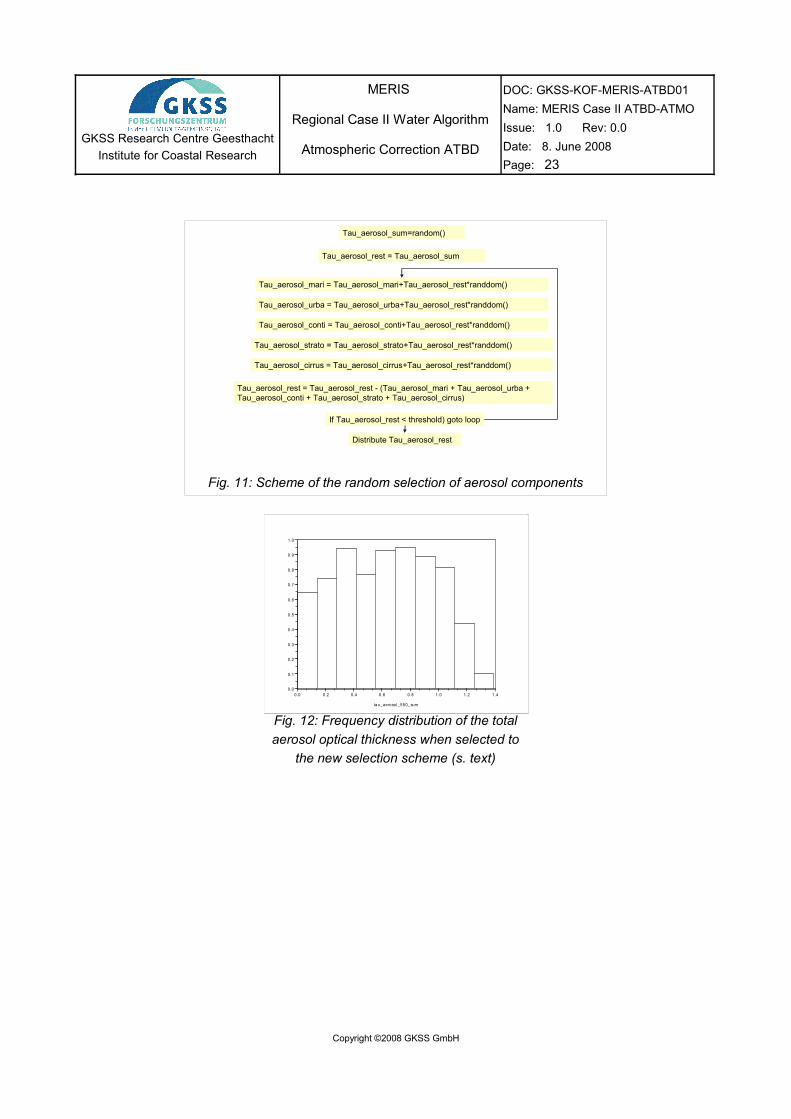
First a total attenuation value is randomly selected from an uniform distribution between 0 and maximum of the total aerosol optical thickness. Then from this value optical thicknesses are selected for each component in a loop until all of the total attenuation is used (Fig. m11). By this selection scheme the overall optical thickness was nearly uniformly distributed. These data were the basis for the generation of the neural network training and test data set using the Monte Carlo photon tracing code (Fig. 12 and 13).


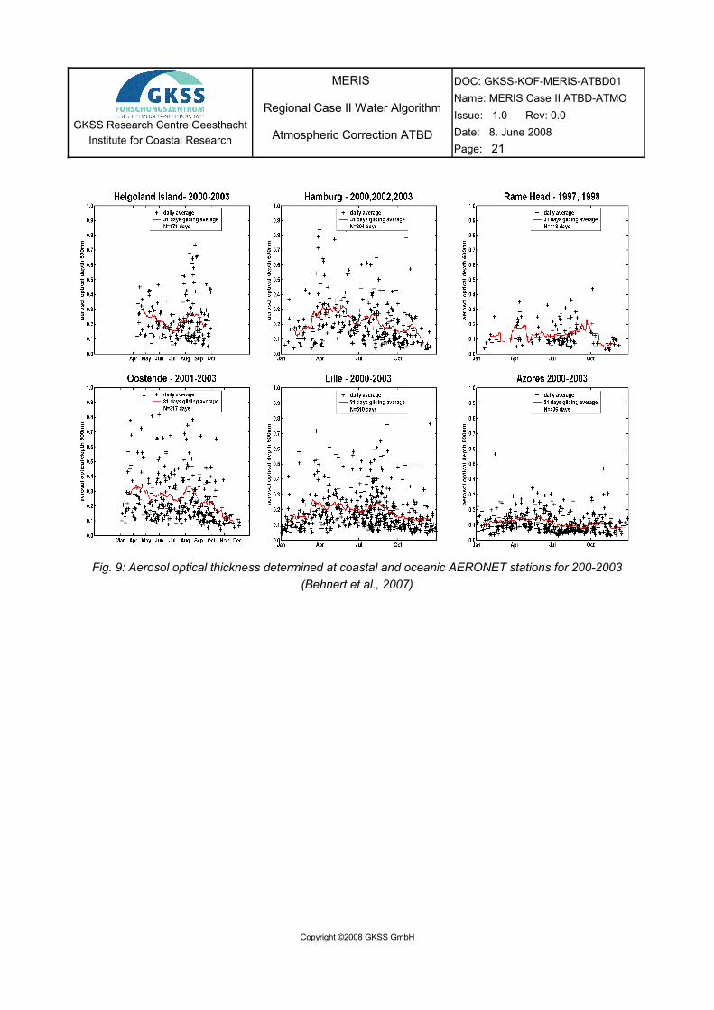
Fig. 10 Angstrom coefficients as measured at different coastal and oceanic sites (AERONET data), which were used as the basis for the coastal aerosol model (Behnert et al., 2007)


MERIS




Fig. 11: Scheme of the random selection of aerosol components

Fig. 12: Frequency distribution of the total aerosol optical thickness when selected to

the new selection scheme (s. text)


Tau_aerosol_sum=random()

Tau_aerosol_rest = Tau_aerosol_sum

Tau_aerosol_mari = Tau_aerosol_mari+Tau_aerosol_rest*randdom()

Tau_aerosol_urba = Tau_aerosol_urba+Tau_aerosol_rest*randdom()

Tau_aerosol_conti = Tau_aerosol_conti+Tau_aerosol_rest*randdom()

Tau_aerosol_strato = Tau_aerosol_strato+Tau_aerosol_rest*randdom()

Tau_aerosol_cirrus = Tau_aerosol_cirrus+Tau_aerosol_rest*randdom()

Tau_aerosol_rest = Tau_aerosol_rest - (Tau_aerosol_mari + Tau_aerosol_urba + Tau_aerosol_conti + Tau_aerosol_strato + Tau_aerosol_cirrus)

If Tau_aerosol_rest < threshold) goto loop

Distribute Tau_aerosol_rest

0.0 0.2 0.4 0.6 0.8 1.0 1.2 1.40.0

0.1

0.2

0.3

0.4

0.5

0.6

0.7

0.8

0.9

1.0

tau_aerosol_550_sum


MERIS





Fig. 13: Range and Frequency distribution for all aerosol components as used for the generation of training data set

0.00 0.05 0.10 0.15 0.20 0 .25 0.30 0.35 0.40 0 .45 0.500.0

0.5

1.0

1.5

2.0

2.5

3.0

3.5

4.0

tau_aerosol_550_ci rrus

0.0000 0.0005 0.0010 0.0015 0.0020 0.0025 0.0030 0.0035 0.0040 0.0045 0.00500

50

100

150

200

250

300

350

400

tau_aerosol_550_strato

0.00 0.05 0.10 0.15 0.20 0 .25 0.300

1

2

3

4

5

6

7

8

tau_ae rosol_550_conti

0.0 0.1 0.2 0.3 0.4 0.5 0.6 0.7 0 .8 0.90.0

0.5

1.0

1.5

2.0

2.5

tau_ae rosol_550_urba

0.00 0.05 0.10 0.15 0.20 0.25 0.30 0.350

1

2

3

4

5

6

tau_aerosol_550_m ari

Tau_mari 0 - 0.2 Tau_urba 0 - 0.5 Tau_conti 0 - 0.18

Tau_strato 0 - 0.003 Tau_cirrus 0 - 0.3


MERIS




Fig. 14 Mixed gas extinction (550 nm) and ozone density profile

Fig. 15 Vertical profile of extinction at 550 nm for different aerosols


0 0.002 0.004 0.006 0.008 0.01 0.012 0.014 0.016 0.018 0.020

5

10

15

20

25

30

35

40

45

50

mixed gas extinc tion c (550) [km-1 ] / ozone dens ity [cm/km]

altitude [km]

ozonemixe d g as

10-6 10-5 10-4 10-3 10-2 10-10

5

10

15

20

25

30

35

40

45

50

aeros ol extinction c(550) [km-1 ]

altitude [km]

urbanmaritimecontine nta ls tratoc irrus


MERIS




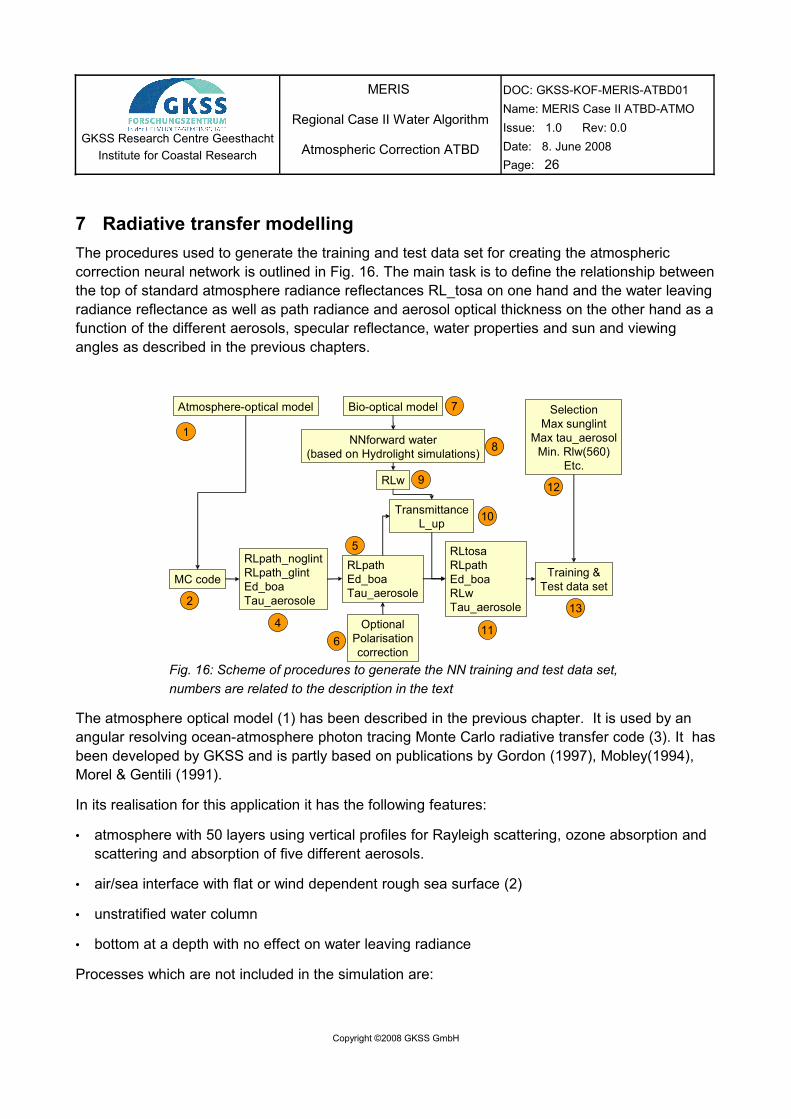
7 Radiative transfer modellingThe procedures used to generate the training and test data set for creating the atmospheric correction neural network is outlined in Fig. 16. The main task is to define the relationship between the top of standard atmosphere radiance reflectances RL_tosa on one hand and the water leaving radiance reflectance as well as path radiance and aerosol optical thickness on the other hand as a function of the different aerosols, specular reflectance, water properties and sun and viewing angles as described in the previous chapters.

Fig. 16: Scheme of procedures to generate the NN training and test data set, numbers are related to the description in the text

The atmosphere optical model (1) has been described in the previous chapter. It is used by an angular resolving ocean-atmosphere photon tracing Monte Carlo radiative transfer code (3). It has been developed by GKSS and is partly based on publications by Gordon (1997), Mobley(1994), Morel & Gentili (1991).

In its realisation for this application it has the following features:

• atmosphere with 50 layers using vertical profiles for Rayleigh scattering, ozone absorption and scattering and absorption of five different aerosols.

• air/sea interface with flat or wind dependent rough sea surface (2)

• unstratified water column

• bottom at a depth with no effect on water leaving radiance

Processes which are not included in the simulation are:


MC code

RLpath_noglintRLpath_glintEd_boaTau_aerosole

NNforward water(based on Hydrolight simulations)

RLw

SelectionMax sunglint

Max tau_aerosolMin. Rlw(560)

Etc.

RLpathEd_boaTau_aerosole

RLtosaRLpathEd_boaRLwTau_aerosole

Bio-optical modelAtmosphere-optical model

OptionalPolarisationcorrection

TransmittanceL_up

Training &Test data set

1

2

46

5

7

8

9

10

11

12

13


MERIS




• polarization

• any inelastic scattering (fluorescence, Raman scattering)

• wind direction

• computation of the water leaving radiance

The detector is positioned just above the water surface for counting the downwelling irradiance and at top of the standard atmosphere to determine the TOSA radiance reflectance for different viewing and solar angles. The angular distribution of radiance is resolved with an angle of 7.5 degrees in azimuth and zenith distance.

Photons start with a weight of 1 for all wavelengths at top of atmosphere (layer 51 of the model atmosphere) from a sun disc of 0.5 degree apparent diameter. The weight is multiplied with the cosine of the sun zenith angle to get the downwelling irradiance Ed_toa. At each collision event the photon weight is multiplied with the single scattering albedo, ωο, of the layer in which the event happens, to take into account for the probability of absorption. The travel distance between two collision events is calculated from a random pull. When the weight is reduced to a value of < 0.01 a "Russian Roulette" decision procedure is started to either end the life of the photon or increase the weight again.

The type of scattering is determined from the concentration mixture of the different media or constituents in water or air. Probability tables for the random pull of the type of scattering are pre-generated for each layer. The scattering angle at each event is randomly pulled from large tables which contain, for each media or constituent, the pre-calculated probabilities for the scattering angle in theta.

The weights of photons, which reach the air/sea interface layer in downwelling direction, are counted for calculating the downwelling vector irradiance.

The wave slope angles are randomly pulled from a probability table, which is calculated using the Cox & Munk (1954) wind (2) dependent sea surface slope distribution. This distribution is isotropic with respect to the azimuth, i.e. it does not take into account the wind direction.

The simulation for one case and one wavelength is completed when a predefined number of photons have reached the radiance detector, i.e. the number of started photons is variable in order to account for strong differences in ωο of different concentrations mixtures and wavelengths. The standard deviation from this photon counting is also recorded. Furthermore, all sun glint photons are labelled and counted separately. They are defined as those photons, which were never scattered in the atmosphere.

Result of the MC simulation (4) are the top of standard atmosphere radiance reflectance, the path radiance reflectance, the sun glint, the downwelling irradiance at bottom of atmosphere and the optical thicknesses for the total and the individual aerosols. Glint and no-glint photons are summed



MERIS




up to get the total path radiance (5). These values can be optionally corrected for the influence of polarisation in the atmosphere and at the water surface (6). This correction is performed by a special neural network, which has been trained with two data sets, one with and the other without considering the polarisation effect in the Monte Carlo run (K. Schiller, 2007, unpublished). However this option is still experimental.

To compute the total radiance reflectance at top of standard atmosphere RL_tosa, the water leaving radiances RLw has to be added to the path radiance reflectances RL_path after its transmittance through the atmosphere t_rlw.

RL_tosa = RL_path + t_rlw * RLw

Although the MC code allows to include the computation of Rlw, by allowing the photons to dive into the water, this feature was not used because of its high computational time requirement. Instead the forward NN (8) of the water retrieval was used to simulate RLw (9). It is based on the same water bio-optical model (7) as used for training of the inverse water NN. This separation of the atmospheric from the water part allows a much higher flexibility and efficiency for generating training data sets for different water conditions. One critical step is the computation of the transmittance of RLw to TOSA (10). It will be described in detail in chapter 9.1. Now all values are computed for the full range of variables (11). However since it is unlikely or impossible that a NN can handle and produce acceptable results for all of these possible cases, a selection is performed for the training of different NN (12). In particular it is necessary to restrict the maximum sun glint contribution and the maximum aerosol optical thickness for cases with highly absorbing water, i.e. with high concentrations of yellow substances and phytoplankton pigments, so that the final training data set (13) is only a subset of the total.

7.1 Computation of the upward directed radiance transmittances

One problem, which is still under debate (s. discussion in the MERIS DQWG), is the proper computation of the transmittance of the upward directed radiance from the water surface to the sensor at top of atmosphere. In the course of this project, initially the transmittance of the downwelling irradiance, which is an output of the neural network, was also applied to compute the transmittance of the upward directed radiance. For this the path length has to be changed according to the different sun and viewing zenith angles. However, low values of the water leaving radiance reflectances indicated that the transmittance of the upward directed radiance might be too high if calculated this way.

As a consequence the upward directed radiance transmittance was simulated using the MC code. Photons were traced from BOA to TOA and only counted at TOA when they arrived at the same 7.5x7.5 degree quad as at BOA. These values were then compared for the nadir cases with the irradiance transmittance.

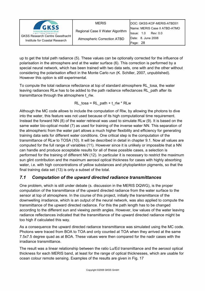
The result was a linear relationship between the ratio Lu/Ed transmittance and the aerosol optical thickness for each MERIS band, at least for the range of optical thicknesses, which are usable for ocean colour remote sensing. Examples of the results are given in Fig. 17



MERIS




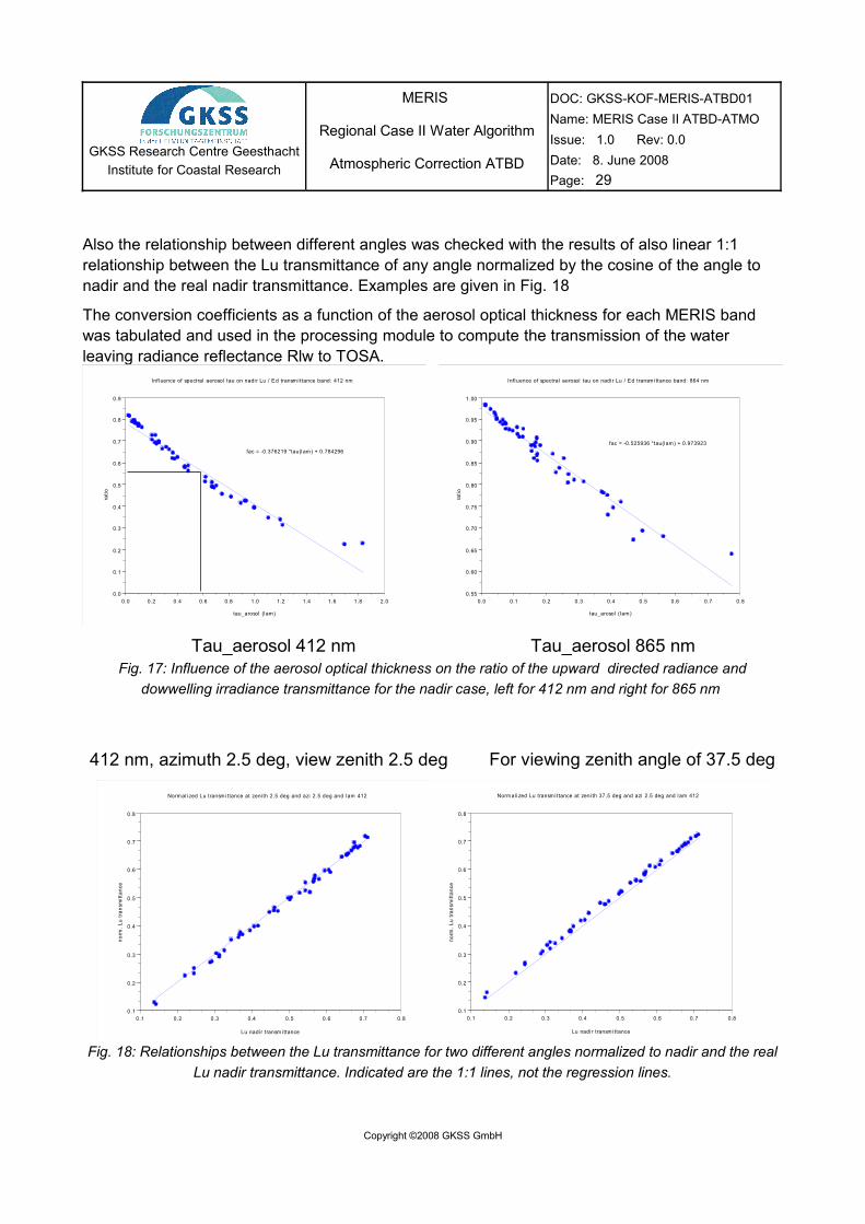
Also the relationship between different angles was checked with the results of also linear 1:1 relationship between the Lu transmittance of any angle normalized by the cosine of the angle to nadir and the real nadir transmittance. Examples are given in Fig. 18

The conversion coefficients as a function of the aerosol optical thickness for each MERIS band was tabulated and used in the processing module to compute the transmission of the water leaving radiance reflectance Rlw to TOSA.


Fig. 17: Influence of the aerosol optical thickness on the ratio of the upward directed radiance and dowwelling irradiance transmittance for the nadir case, left for 412 nm and right for 865 nm

fac = -0.376219 *tau(l am) + 0.784296

0.0 0.2 0.4 0.6 0.8 1.0 1.2 1.4 1.6 1.8 2.00.0

0.1

0.2

0.3

0.4

0.5

0.6

0.7

0.8

0.9

Infl uence of spectral aerosol tau on nadi r Lu / Ed transm i ttance band: 412 nm

tau_arosol (l am)

ratio

fac = -0.525936 *tau(l am) + 0.973923

0.0 0.1 0.2 0.3 0.4 0.5 0.6 0.7 0.80.55

0.60

0.65

0.70

0.75

0.80

0.85

0.90

0.95

1.00

Influence of spectral aerosol tau on nadi r Lu / Ed transmi ttance band: 864 nm

tau_arosol (l am)

ratio

Tau_aerosol 412 nm Tau_aerosol 865 nm

Fig. 18: Relationships between the Lu transmittance for two different angles normalized to nadir and the real Lu nadir transmittance. Indicated are the 1:1 lines, not the regression lines.

0.1 0.2 0.3 0.4 0.5 0.6 0.7 0.80.1

0.2

0.3

0.4

0.5

0.6

0.7

0.8

Norm al i zed Lu transm i ttance at zeni th 2.5 deg and azi 2.5 deg and l am 412

Lu nadi r transm i ttance

norm

. Lu

trans

mitt

ance

0.1 0.2 0.3 0.4 0.5 0.6 0.7 0.80.1

0.2

0.3

0.4

0.5

0.6

0.7

0.8

Norm al i zed Lu transm i ttance at zeni th 37.5 deg and azi 2.5 deg and l am 412

Lu nadi r transmi ttance

norm

. Lu

trans

mitt

ance

412 nm, azimuth 2.5 deg, view zenith 2.5 deg For viewing zenith angle of 37.5 deg


MERIS




7.2 Wavelengths used for simulations

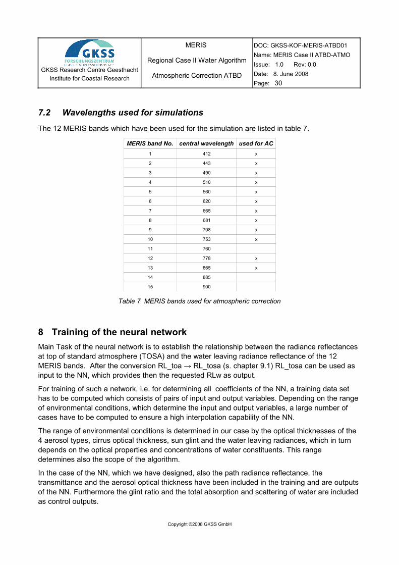
The 12 MERIS bands which have been used for the simulation are listed in table 7.

MERIS band No. central wavelength used for AC1 412 x

2 443 x

3 490 x

4 510 x

5 560 x

6 620 x

7 665 x

8 681 x

9 708 x

10 753 x

11 760

12 778 x

13 865 x

14 885

15 900

Table 7 MERIS bands used for atmospheric correction

8 Training of the neural networkMain Task of the neural network is to establish the relationship between the radiance reflectances at top of standard atmosphere (TOSA) and the water leaving radiance reflectance of the 12 MERIS bands. After the conversion RL_toa → RL_tosa (s. chapter 9.1) RL_tosa can be used as input to the NN, which provides then the requested RLw as output.

For training of such a network, i.e. for determining all coefficients of the NN, a training data set has to be computed which consists of pairs of input and output variables. Depending on the range of environmental conditions, which determine the input and output variables, a large number of cases have to be computed to ensure a high interpolation capability of the NN.

The range of environmental conditions is determined in our case by the optical thicknesses of the 4 aerosol types, cirrus optical thickness, sun glint and the water leaving radiances, which in turn depends on the optical properties and concentrations of water constituents. This range determines also the scope of the algorithm.

In the case of the NN, which we have designed, also the path radiance reflectance, the transmittance and the aerosol optical thickness have been included in the training and are outputs of the NN. Furthermore the glint ratio and the total absorption and scattering of water are included as control outputs.



MERIS




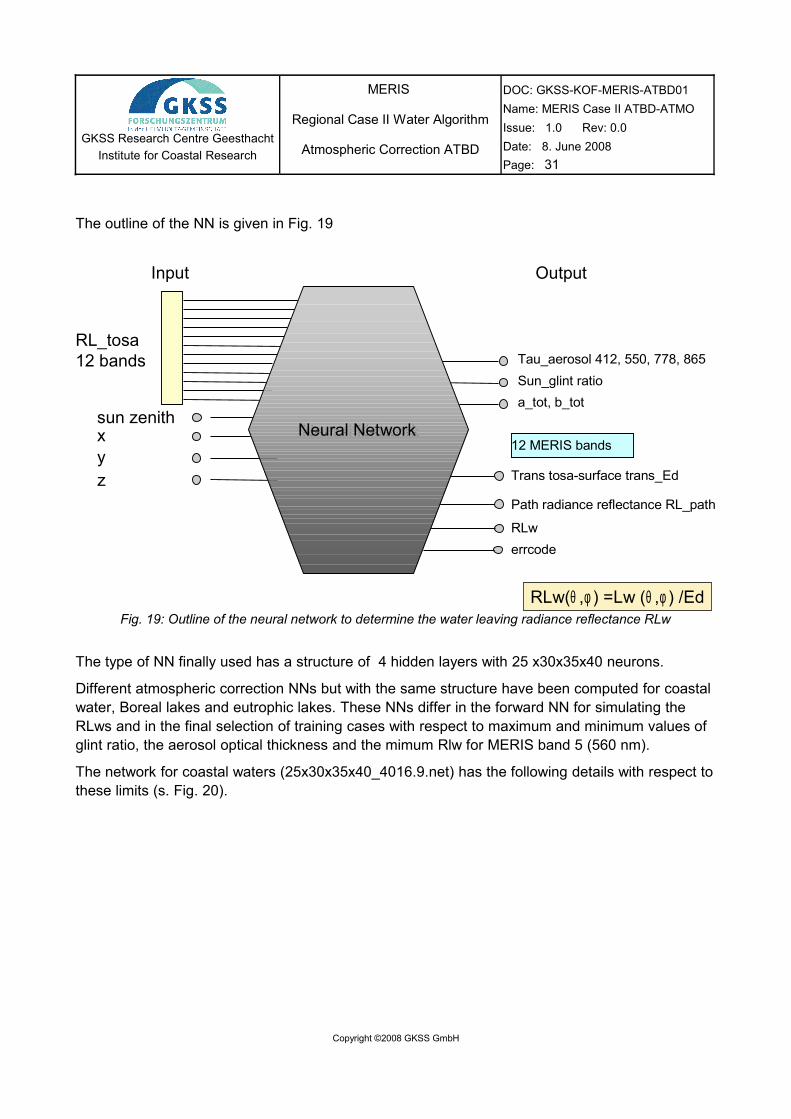
The outline of the NN is given in Fig. 19

The type of NN finally used has a structure of 4 hidden layers with 25 x30x35x40 neurons.

Different atmospheric correction NNs but with the same structure have been computed for coastal water, Boreal lakes and eutrophic lakes. These NNs differ in the forward NN for simulating the RLws and in the final selection of training cases with respect to maximum and minimum values of glint ratio, the aerosol optical thickness and the mimum Rlw for MERIS band 5 (560 nm).

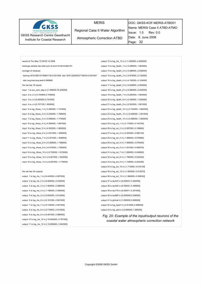
The network for coastal waters (25x30x35x40_4016.9.net) has the following details with respect to these limits (s. Fig. 20).


Fig. 19: Outline of the neural network to determine the water leaving radiance reflectance RLw

Neural Networksun zenith

Path radiance reflectance RL_path

Trans tosa-surface trans_Ed

RLw

RL_tosa12 bands

12 MERIS bandsxy

Input Output

RLw(θ ,φ ) =Lw (θ ,φ ) /Ed

Tau_aerosol 412, 550, 778, 865Sun_glint ratioa_tot, b_tot

errcode

z

Neural Network


MERIS





saved at Thu May 15 09:02:14 2008

trainings sample has total sum of error^2=4016.882157

average of residues:

training 4016.882157/59947/16=0.001558 test 1876.324555/27158/43=0.001607

ratio avg.train/avg.test=0.969865

the net has 16 inputs:

input 1 is sun_zeni_deg in [1.008000,76.200000]

input 2 is x in [-0.704900,0.705600]

input 3 is y in [0.000002,0.707000]

input 4 is z in [0.707100,1.000000]

input 5 is log_rltosa_1 in [-3.265000,-1.747000]












the net has 43 outputs:

output 1 is log_rlw_1 in [-8.443000,-2.087000]












output 13 is log_rlpath_1 in [-3.299000,-1.963000]












output 25 is log_ed_1 in [-2.172000,-0.142700]












output 37 is tau443 in [0.000031,0.462000]

output 38 is tau550 in [0.000021,0.299900]

output 39 is tau778 in [0.000011,0.267000]

output 40 is tau865 in [0.000009,0.258000]

output 41 is glintrat in [1.000000,5.999000]

output 42 is log_bpart in [-2.814000,3.999000]

output 43 is log_atot in [-6.900000,1.380000]

Fig. 20: Example of the input/output neurons of the coastal water atmsopheric correction network


MERIS




8.1 The training of the atmospheric correction NN

The Monte Carlo model was used to calculate the top of standard atmosphere path radiance reflectances and the downwelling irradiance at sea level. The ranges of interest of the variables were defined to be those given in Table 6. The values were chosen to cover a large range of ocean, coastal and land aerosols and cirrus clouds. However, different trials demonstrated that it was necessary to limit e.g. the maximum optical thickness and sun glint to values, where the water leaving radiance reflectance is still detectable within the RL_tosa spectrum. For the 25x30x35x40_4016.9.net NN the maximum aerosol optical thickness at 550 nm was set to 0.3 and the maximum sun glint ratio to 6.0.

First 11695 cases of path radiances and irradiances were computed with randomly selected sun zenith distances, wind speeds and sun glint, aerosols and cirrus clouds. For each case 7 viewing angles were randomly selected. Then for each of these 81865 cases 5 different water leaving radiances were added, which were also randomly computed as described above. From these 409325 spectra a selection was made with respect to maxima values of sun glint and tau550 of aerosols to build the final training data set. About 66% of these data are used for training, the other 34 % are used for testing during the training process in order to avoid overtraining. Thus it is constantly checked that the error of the training data set is similar to that of the test data set.

The software which was used for training the NN is the GKSS Neural Network Simulator FFBP v1.0 (Schiller, 1997). The NN is fully connected (each `neurone' of a layer is connected with each `neuron' of the following layer) and is initialised by assigning random numbers (uniformly in (0,1)) to the weights and biases.

For error-minimisation the backpropagation method with momentum and flat spot term was used. The `teaching'-sample was applied to the ffNN in random order. At start the control parameters were set as follows: learning factor 0.6, momentum factor 0.2 and flat spot term 0.02. Each time if the error-function did not decrease any more the minimisation-parameters were divided by 3. The minimisation was continued until the error function was down to an average output error of 1.5%.

The weights and biases obtained by `teaching' of the ffNN were used to generate a table including parameters of the architecture of the NN and all coefficients. An interface routine reads this table and constructs the network in a preparatory set-up step before using the net pixel by pixel. Also the backtransformation from the (0,1)-interval for the components are built into this function.

8.2 The performance of the NN

The performance of the NN can be assessed when using the input data from the test data set and comparing the output of the NN with the expected values from the output values of the test data set.

As an example the results are given here for the coastal water NN, 25x30x35x40_4016.9.net (Fig. 21-24).



MERIS




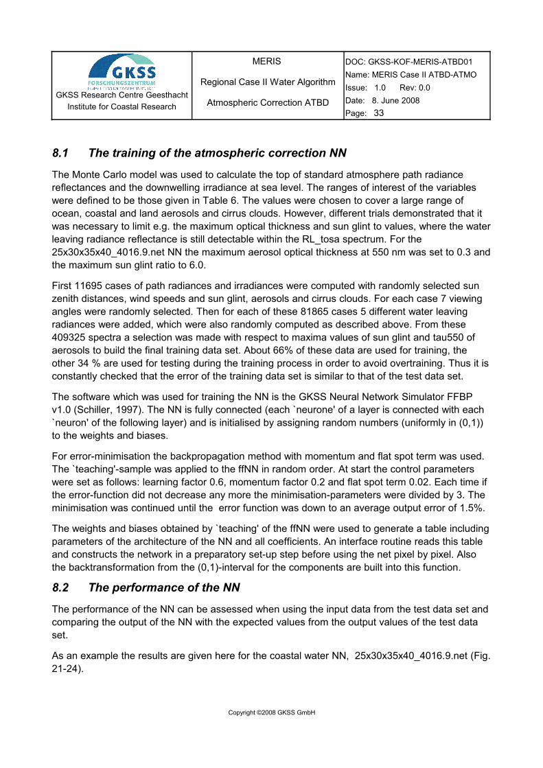
From these results it is obvious, that the uncertainty increases as expected with decreasing RLw. This is particular the case under hazy conditions. Here values < 0.001 cause already problems. Consequence for highly absorbing water types, such as many lakes in Finland with concentrations of yellow substances but low concentrations of scattering particles, it is not possible to determine the water leaving radiance under conditions with an aerosol optical thickness around > 0.2.

.

Fig. 21: Test of the NN for log_RLw band 1 (412 nm) and band 9 (708 nm). Target is the correct value of the model output, actual is the output of the NN.

Fig. 22: Test of the NN for log_RL_path band 1 (412 nm) and band 9 (708 nm). Target is the correct value of the model output, actual is the output of the NN.



MERIS




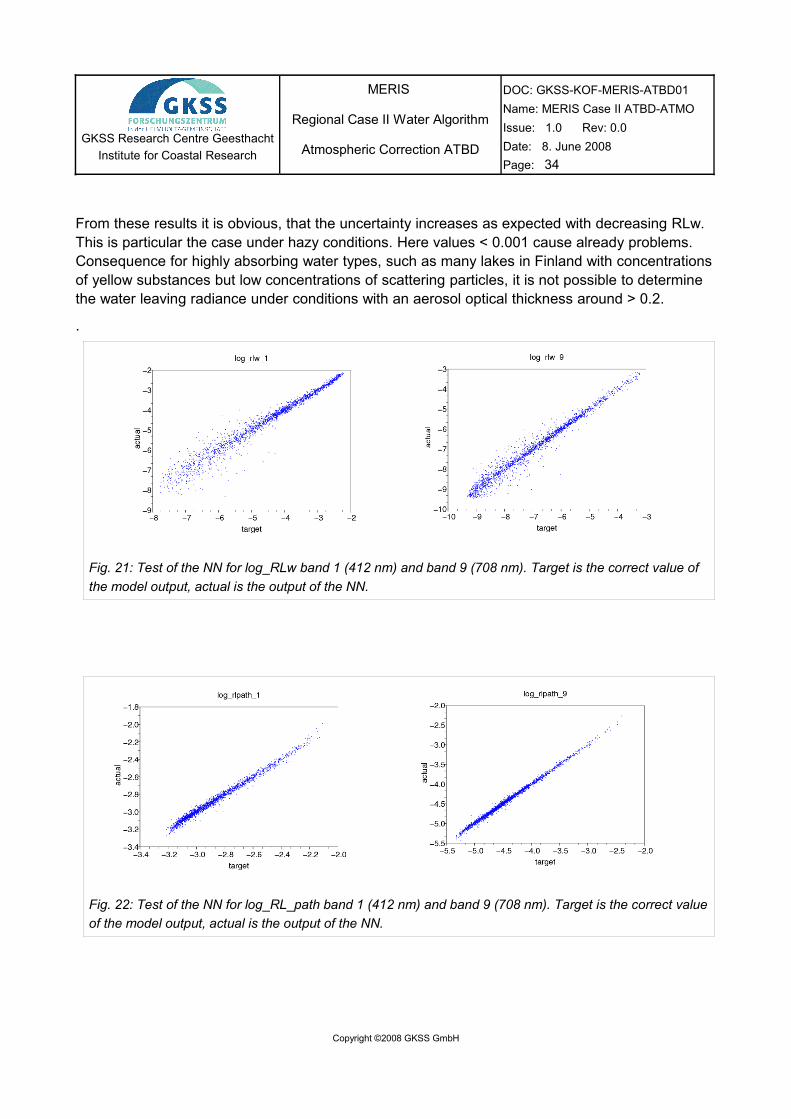
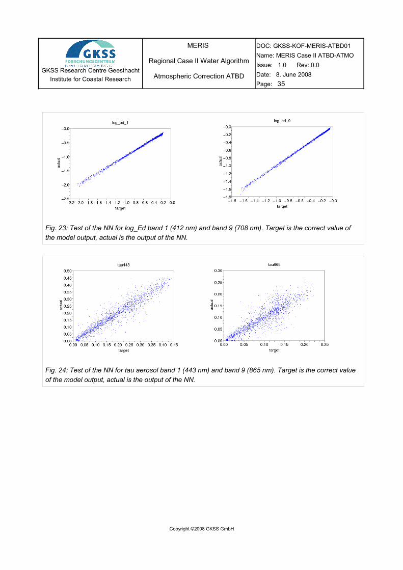
Fig. 23: Test of the NN for log_Ed band 1 (412 nm) and band 9 (708 nm). Target is the correct value of the model output, actual is the output of the NN.

Fig. 24: Test of the NN for tau aerosol band 1 (443 nm) and band 9 (865 nm). Target is the correct value of the model output, actual is the output of the NN.



MERIS




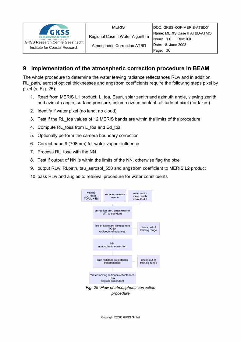
9 Implementation of the atmospheric correction procedure in BEAMThe whole procedure to determine the water leaving radiance reflectances RLw and in addition RL_path, aerosol optical thicknesses and angstrom coefficients require the following steps pixel by pixel (s. Fig. 25):

1. Read from MERIS L1 product: L_toa, Esun, solar zenith and azimuth angle, viewing zenith and azimuth angle, surface pressure, column ozone content, altitude of pixel (for lakes)

2. Identify if water pixel (no land, no cloud)

3. Test if the RL_toa values of 12 MERIS bands are within the limits of the procedure

4. Compute RL_tosa from L_toa and Ed_toa

5. Optionally perform the camera boundary correction

6. Correct band 9 (708 nm) for water vapour influence

7. Process RL_tosa with the NN

8. Test if output of NN is within the limits of the NN, otherwise flag the pixel

9. output RLw, RLpath, tau_aerosol_550 and angstrom coefficient to MERIS L2 product

10. pass RLw and angles to retrieval procedure for water constituents

MERISL1 data

TOA L + Edsurface pressure

ozonesolar zenithview zenithazimuth diff

correction atm. press+ozonediff. to standard

Top of Standard AtmosphereTOSA

radiance reflectances

NNatmospheric correction

path radiance reflectancetransmittance

Water leaving radiance reflectancesRLw

angular dependent

check out oftraining range

solar zenithview zenithazimuth diff

check out oftraining range

Fig. 25 Flow of atmospheric correction procedure



MERIS




9.1 Computation of RL_tosa from RL_toa

The top of standard atmosphere (TOSA) with respect to air pressure and ozone column content has been introduced in order not to overload the NN with too many variables. Since the influence of the difference between standard values and the actual values of a pixel concerning Rayleigh scattering and ozone absorption are small and can be decoupled only the standard values have been used for the simulation of the training data set for the NN. By this the interaction between different Rayleigh-Mie scattering events in the atmosphere is nearly fully preserved.

According to the true structure of the atmosphere the ozone correction layer is put on top of the Rayleigh correction layer. The Rayleigh correction includes differences from the standard ground pressure of 1013.2 hPa concerning air pressure variations at ground and for inland waters also determined by the altitude. All three variables, i.e. ground pressure, ozone content, altitude, are taken from the MERIS L1b data.

The calculations for ozone and Rayleigh scattering are according to André & Morel (1989).

First, RL_toa, the radiance reflectance at TOA, is calculated from the solar irradiance, sun_toa, (taken from MERIS L1b data) and the cosine of the sun zenith angle for that pixel, cos_teta_sun, with Ed_toa, the downwelling irradiance at TOA.

Ed_toa = sun_toa*cos_teta_sun;

RL_toa = L_toa/Ed_toa;

9.1.1 Correction for ozoneThe first correction regards the ozone correction layer. The ozone mass for correction is the difference between the standard value of 0.35 cm == 350 Dobson units, and the actual column content, pixel_ozon, which is taken from the MERIS L1b data. Since this value is given in Dobson units, it has to be divided by 1000 to get the value in cm ozone at surface pressure:

ozon_rest_mass = (pixel_ozon / 1000.0 - 0.35);

The transmittances for the solar irradiance, trans_oz_toa_tosa_down, and the upward radiance, trans_oz_toa_tosa_up, with the specific wavelength (lam) dependent absorption coefficient per cm, constants_absorb_ozon(lam) , through the ozone correction layer are then:

trans_oz_toa_tosa_down = exp(-constants_absorb_ozon(lam) * ozon_rest_mass / cos_teta_sun);

trans_oz_toa_tosa_up = exp(-constants_absorb_ozon(lam) * ozon_rest_mass / cos_teta_view);

9.1.2 Correction for Rayleigh scatteringThe actual pressure at ground of the pixel is computed from the pixel_pressure and the pixel_altitude, as taken from the MERIS L1b product, according to the standard height-pressure formulation.



MERIS




altitude_pressure = pixel_pressure*(1.0 – 0.0065 * pixel_altitude / 288.15)^5.255;

The relative air mass for the difference TOA-TOSA relevant for the correction is then:

rayl_rel_mass_toa_tosa = (altitude_pressure -1013.2) / 1013.2;

For sea level and a surface pressure of < 1013.2 hPa this relative air mass can become also negative.

The optical thickness of the layer TOA-TOSA, tau_rayl_toa_tosa, is then computed according to the standard Rayleigh formula:

tau_rayl_standard = 0.008735 * (wavelength_nm / 1000.0)^( -4.08); // lam in µm */

tau_rayl_toa_tosa = tau_rayl_standard * rayl_rel_mass_toa_tosa;

Now the transmittances for the downwelling irradiance TOA-TOSA and the upwelling radiance TOSA-TOA can be computed by using the corresponding angles for that pixel:

trans_rayl_toa_tosa_down = exp(-tau_rayl_toa_tosa * 0.5 / cos_teta_sun);

trans_rayl_toa_tosa_up = exp(-tau_rayl_toa_tosa * 0.5 / cos_teta_view);

The factor 0.5 is used because of the symmetric phase function of Rayleigh scattering.

For the calculation of the path radiance of the TOA-TOSA layer first the angle, cos_scat_ang, for the Rayleigh phase function, phase_rayl, has to be computed:

cos_scat_ang = -cos_teta_view * cos_teta_sun - sin_teta_view * sin_teta_sun * cos_azi_diff;

phase_rayl = 0.75 * (1.0 + cos_scat_ang * cos_scat_ang);

The path radiance, L_rcpath, of the layer is then:

L_rcpath = Ed_toa * tau_rayl_toa_tosa * trans_oz_tosa_down* phase_rayl / (4*PI * cos_teta_view * cos_teta_sun);

The downelling irradiance, Ed_tosa, and the upwelling radiance, L_tosa, become:

Ed_tosa = Ed_toa * trans_oz_toa_tosa_down * trans_rayl_toa_tosa_down;

L_tosa = (L_toa - L_rcpath*trans_oz_tosa_up)/ (trans_rayl_toa_tosa_up*trans_oz_toa_tosa_up) ;

Finally we get the required radiance reflectance RL_tosa by:

RL_tosa = L_tosa/ Ed_tosa ;

9.2 Correction of water vapour influence on MERIS band 9 708 nm

The correction for water valpour absorption is necessary for MERIS band 9 (708 nm) , because



MERIS




this band reaches partly into one of the water vapour absorption bands of the atmosphere.

For the correction MERIS bands 14 and 15 are used, which are dedicated to the determination of the water vapour. The correction is performed as in the MERIS IPF ground processor. The coefficients are taken from the corresponding LUTS of the IPF.

The polynom coefficients H2O_COR_POLY are: 0.3832989, 1.6527957, -1.5635101, 0.5311913.

The reflectances for band 14, rho_885, and band 15, rho_900, are computed directly from the radiances and solar flux as taken from the MERIS L1b product:

rho_885 = pixel.toa_radiance_885 / solar_flux_885;

rho_900 = pixel.toa_radiance_900 / pixel.solar_flux_900;

x2 = rho_900 / rho_885;

The transmittance for band 9, trans708, is then computed by using the polynomial coefficients:

trans708 = H2O_COR_POLY[0] + H2O_COR_POLY[1] * x2 + H2O_COR_POLY[2] * x2 * x2 + H2O_COR_POLY[3] * x2 * x2 * x2;

Finally RL_tosa is corrected by:

RL_tosa = RL_tosa / trans708;

9.3 Use of cartesian coordinates

The atmospheric correction is very sensitive against errors regarding the sun and viewing angles, in particular because of the specular reflectance at the sea surface (sky and sun glint). The viewing angles of MERIS around the nadir are not well determined because of the jump in azimuth direction. The viewing azimuth angle is interpolated from the anchor points. When using the azimuth viewing angles as provided in the MERIS L1b data in BEAM, artefacts in the image occur in form of a vertical broad smooth band around the nadir line.

In order to avoid this artefact, the angles have been converted into cartesian coordinates:

x = -sin(teta_view_rad) * cos(azi_diff_rad);

y = abs(-sin(teta_view_rad) * sin(azi_diff_rad));

z = cos(teta_view_rad);

These values are then input to the atmospheric correction neural network, which has been trained also with cartesian coordinates.

Furthermore, before this conversion, one has to consider that the azimuth angles and the corresponding azimuth difference are differently defined in the MERIS product and the simulation model.



MERIS




9.4 Computation of the angstrom coefficient

The aerosol optical thicknesses for four wavelength, tau443, tau550, tau778, tau865, are a direct output of the atmospheric correction NN.

The angstrom coefficient is then computed from tau443 and tau865:

ang_443_865 = log(tau443/tau865) / log(443/865);

9.5 Correction of camera boundary problem (“smile effect”)

A full swath of MERIS is composed of the swath of the 5 MERIS cameras. In some of the products the boundaries between the cameras are visible and cause also jumps in the derived concentrations. The causes for these boundaries are not fully known in detail. One reason is the alignment of the 5 sensor CCD chips. Because of small misalignments, which are different from camera to camera, there is shift in the projected wavelength, so that at the contiguous sides of two cameras have different wavelengths, which cause changes in the product. Since this wavelength shift has a significant influence on the computation of the Rayleigh scattering, the correction of the camera boundary was included into the atmospheric correction part of the BEAM case 2 water processor.

However, since the camera alignment is obviously not the only cause for the camera boundary problem, the correction as included here, does not fully solve the problem. There are sometimes even cases, where the correction makes the camera boundaries even more visible. Thus, the camera boundary correction procedure can be optionally switched on by a parameter in the parameter file. Another reason for the boundary problem is probably different stray light in the cameras, which depends on the targets the camera is pointing at. This possible cause is still under investigation by the MERIS Data Quality Working Group of ESA and no procedure for correction of this stray light is presently available.

In the atmospheric correction processor, as described here, only the correction for the wavelength shift regarding the solar irradiance and the Rayleigh scattering are treated.

For this purpose the look-up tables for the true wavelength per pixel along the full swath (different for FR and RR mode) are used, as provided by ESA. These wavelength are identified by the pixel numbers, which are provided with the MERIS L1b data.

For each pixel the deviation between the nominal wavelength and the actual wavelength is used to compute the difference in Rayleigh path radiance and solar irradiance. These differences are then treated in the same way as the difference between TOA and TOSA atmosphere.



MERIS




10 ReferencesAndré, J.M. and A. Morel (1989). Simulated effects of barometric pressure and ozone content upon the estimate of marine phytoplankton from space, Journal of Geophysical Research, 94, 1029-1037.

André, J.M. and A. Morel (1991). Atmospheric corrections and interpretation of marine radiances in CZCS imagery, revisited, Oceanologica Acta, 14, 3-22.

Ångström, A (1964): The parameters of atmospheric turbidity, Tellus, 26, 64-75

Antoine, D. and Morel, A., 1998, Relative importance of multiple scattering by air molecules and aerosols in forming the atmospheric path radiance in the visible and near-infrared parts of the spectrum, Applied Optics, 37, 2245-2259.

Antoine, D. and A. Morel (1999). A multiple scattering algorithm for atmospheric correction of remotely-sensed ocean colour (MERIS instrument) : principle and implementation for atmospheres carrying various aerosols including absorbing ones, International Journal of Remote Sensing, 20, 1875-1916.

Behnert, Irina, Matthias, Volker, Doerffer, Roland (2007): Aerosol climatology from ground-based measurements for the southern North Sea, Atmospheric Res., 2007

Cox, C., and W. Munk (1954): Statistics of the sea surface derived from Sun glitter. Journal of Marine Research, 13, 198-227

Doerffer R, Fischer J (1994) Concentrations of chlorophyll, suspended matter, and gelbstoff in case II waters derived from satellite coastal zone color scanner data with inverse modeling methods. Journal Geophysical Research 99:7457-7466

Doerffer, R. and H. Schiller (2007): The MERIS Case 2 water algorithm, International Journal of Remote Sensing, Vol. 28, Nos. 3-4, 2007, pp 517-535, 2007.

Eltermann, L. (1968): UV, visible, and IR attenuation for altitudes to 50 km. Environmental Research Paper No. 285, AFCRL-68-0153, Airforce Cambridge Research Laboratories

Elouraginia, Salem, Houda Chtiouia, and Pierre H. Flamant (2005): Lidar remote sounding of cirrus clouds and comparison of simulated fluxes with surface and METEOSAT observations, Atmospheric Research, Volume 73, Issues 1-2, January 2005, Pages 23-36

Gordon, H.R., and A. Morel (1983). Remote assessment of ocean color for interpretation of satellite visible imagery. A review, Springer-Verlag, New York (USA).

Gordon, H.R. : Atmospheric Correction of Ocean Color Imagery in the Earth Observing System Era, Jour. Geophys. Res., 102D, 17081-17106 (1997).

Heinemann, Thomas and Lothar Schüller (1995): MIE-Programmpaket für Strahlungstransportsimulaltionen mit MOMO, Institut für Weltraumwissenschaften, Freie



MERIS




Universität Berlin

Krasnopolsky, V. and H. Schiller (2003): Some Neural Network applications in environmental sciences part I: forward and inverse problems in geophysical remote measurements, Neural Networks, vol 16 (2003), 321-334.

Macke A, Müller J, Raschke E (1996) Single scattering properties of atmospheric ice crystals. Journal of Atmospheric Sciences 53, 2813-2825

Morel, A., and B. Gentili (1991). Diffuse reflectance of oceanic waters: its dependance on sun angle as influence by molecular scattering contribution. Applied Optics, 30, 4427-4438

Mitchell D, Macke A, Liu, Y (1996) Modelling cirrus clouds. part II: Treatment of radiative properties. Journal of Atmospheric Sciences 53, 2967-2988.

Mobley, C.D., Light and Water; Radiative Transfer in Natural Waters (Academic Press, San Diego, Calif., 1994).

Schiller H, Doerffer R (1993) Fast computational scheme for inverse modeling of multispectral radiances: application for remote sensing of the ocean. Applied Optics 32:3280-3285

Schiller, Helmut and Roland Doerffer, 1999, Neural Network for Emulation of an Inverse Model --- Operational Derivation of Case II Water Properties from MERIS data; Int. Journal of Remote Sensing, vol. 20, No 9,1735—1746.

Shettle, E.P. & R. W. Fenn (1979): Models for the aerosols of the lower atmosphere and the effects of humidity variations on their optical properties. Environmental Research Paper No. 676, AFGL-TR-79-0214, Airforce Geophysics Laboratory

World Climate Research Program (WCRP), (1986): A preliminary cloudless standard atmosphere for radiation computation. International Association for Meteorology and Atmsopheric Physics, Radiation Commission, Boulder, CO, USA, 1984, CSP-112, WMO/TD-No. 24, March 1986


Algorithm Theoretical Basis Document (ATBD) · PDF fileconstituents or to provide the inherent...

Documents

Transcript of Algorithm Theoretical Basis Document (ATBD) · PDF fileconstituents or to provide the inherent...