Algorithm for Robust Gear Design · Profile modifications have an effect on the gear strength...
16
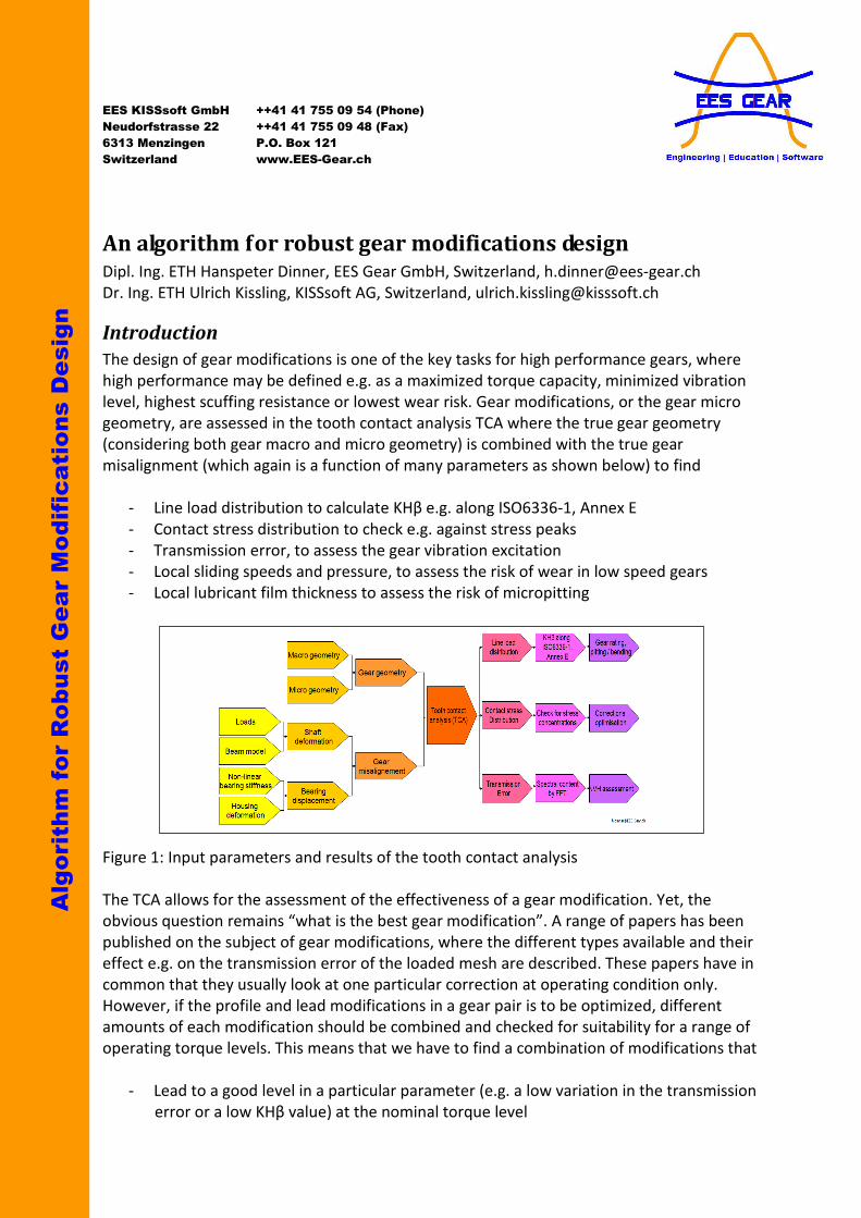
EES KISSsoft GmbH ++41 41 755 09 54 (Phone) Neudorfstrasse 22 ++41 41 755 09 48 (Fax) 6313 Menzingen P.O. Box 121 Switzerland www.EES-Gear.ch An algorithm for robust gear modifications design Dipl. Ing. ETH Hanspeter Dinner, EES Gear GmbH, Switzerland, [email protected] Dr. Ing. ETH Ulrich Kissling, KISSsoft AG, Switzerland, [email protected] Introduction The design of gear modifications is one of the key tasks for high performance gears, where high performance may be defined e.g. as a maximized torque capacity, minimized vibration level, highest scuffing resistance or lowest wear risk. Gear modifications, or the gear micro geometry, are assessed in the tooth contact analysis TCA where the true gear geometry (considering both gear macro and micro geometry) is combined with the true gear misalignment (which again is a function of many parameters as shown below) to find - Line load distribution to calculate KHβ e.g. along ISO6336-1, Annex E - Contact stress distribution to check e.g. against stress peaks - Transmission error, to assess the gear vibration excitation - Local sliding speeds and pressure, to assess the risk of wear in low speed gears - Local lubricant film thickness to assess the risk of micropitting Figure 1: Input parameters and results of the tooth contact analysis The TCA allows for the assessment of the effectiveness of a gear modification. Yet, the obvious question remains “what is the best gear modification”. A range of papers has been published on the subject of gear modifications, where the different types available and their effect e.g. on the transmission error of the loaded mesh are described. These papers have in common that they usually look at one particular correction at operating condition only. However, if the profile and lead modifications in a gear pair is to be optimized, different amounts of each modification should be combined and checked for suitability for a range of operating torque levels. This means that we have to find a combination of modifications that - Lead to a good level in a particular parameter (e.g. a low variation in the transmission error or a low KHβ value) at the nominal torque level Algorithm for Robust Gear Modifications Design
Transcript of Algorithm for Robust Gear Design · Profile modifications have an effect on the gear strength...
EES KISSsoft GmbH ++41 41 755 09 54 (Phone)
Neudorfstrasse 22 ++41 41 755 09 48 (Fax)
6313 Menzingen P.O. Box 121
Switzerland www.EES-Gear.ch
An algorithm for robust gear modifications design Dipl. Ing. ETH Hanspeter Dinner, EES Gear GmbH, Switzerland, [email protected]
Dr. Ing. ETH Ulrich Kissling, KISSsoft AG, Switzerland, [email protected]
Introduction
The design of gear modifications is one of the key tasks for high performance gears, where
high performance may be defined e.g. as a maximized torque capacity, minimized vibration
level, highest scuffing resistance or lowest wear risk. Gear modifications, or the gear micro
geometry, are assessed in the tooth contact analysis TCA where the true gear geometry
(considering both gear macro and micro geometry) is combined with the true gear
misalignment (which again is a function of many parameters as shown below) to find
- Line load distribution to calculate KHβ e.g. along ISO6336-1, Annex E
- Contact stress distribution to check e.g. against stress peaks
- Transmission error, to assess the gear vibration excitation
- Local sliding speeds and pressure, to assess the risk of wear in low speed gears
- Local lubricant film thickness to assess the risk of micropitting
Figure 1: Input parameters and results of the tooth contact analysis
The TCA allows for the assessment of the effectiveness of a gear modification. Yet, the
obvious question remains “what is the best gear modification”. A range of papers has been
published on the subject of gear modifications, where the different types available and their
effect e.g. on the transmission error of the loaded mesh are described. These papers have in
common that they usually look at one particular correction at operating condition only.
However, if the profile and lead modifications in a gear pair is to be optimized, different
amounts of each modification should be combined and checked for suitability for a range of
operating torque levels. This means that we have to find a combination of modifications that
- Lead to a good level in a particular parameter (e.g. a low variation in the transmission
error or a low KHβ value) at the nominal torque level
Algorithm for Robust Gear Modifications Design
- Result in little variation in the level of this particular parameter if the torque level
changes, meaning, it is a robust design
Furthermore, the different modifications in lead and profile direction may be combined in
any manner and it may not always be intuitive which combination is the best. A suitable
solution to the above problem is to calculate the TCA for different combinations of
modifications, for different sizes of the respective modification and for different load levels
automatically. Then, for each combination, parameters of interest (e.g. PPTE or KHβ) are
found and may be assessed by the gear designer. This also means that the final selection of
the “best” solution is up to the gear designer and is not left for the calculation algorithm to
decide, as the importance of each parameter is, remains and has to be a subjective choice
based on experience and design philosophy. While this approach is not highly refined, it
shows to be highly effective as the below examples will illustrated.
Profile modifications
Profile modifications are either limited to the root or tip area or cover the whole tooth
height. The former are called tip and root relief, and different types are possible. The later
may be a pressure angle modification or profile crowning. The definition of profile
corrections may be found in ISO21771:2007.
Profile modifications have an effect on the gear strength rating along ISO6336:2006 in the
sense that they affect the theoretical contact ratio and hence the contact stress under load.
However, it is recommended not to consider the profile modifications in the gear rating for
pitting and bending. Furthermore, they have a considerable effect on the scuffing rating e.g.
along ISO/TR13989:2000 where they much affect the flash temperature at the start and end
of mesh. They also have an effect on micropitting rating, e.g. along ISO15144:2010, method
B where the profile modifications are considered. If method A (where the local contact
pressure from a tooth contact analysis is used to calculate the EHD film thickness) is used,
then, obviously, the profile modifications have a direct influence as they affect the contact
stresses calculated.
In case of poorly lubricated gears such as dry running plastic gears or slow running, highly
loaded girth gears they strongly affect the local pressure, in particular at the start and end of
mesh and hence the wear rate. Furthermore, profile corrections are applied to avoid point-
surface-origin macropitting in the root of a driving pinion [8].
Another focus of the profile modifications typically is to design them such that the vibration
excitation during the gear meshing is minimized even if load levels centre distance and gear
quality vary. This excitation is typically assessed by means of the variation of the
transmission error, the peak to peak transmission error PPTE and it’s Fourier analysis or the
variation of the resulting meshing / bearing reaction forces (as the bearing forces ultimately
are responsible for housing excitation), see e.g. [1], [3], [4], [5].

Figure 2: Left: Profile modification in K-chart (blue) and permissible error (red). A barreling is
superimposed with a progressive tip relief. Right: Linear tip and root relief definition along
ISO21771:2007.
Lead modifications
Typically, three types of lead modifications are combined in a mesh as listed below. Each of
them serves a distinctive, different purpose
1) Helix angle modification: account for the shaft deflection at design load level
2) Crowning: account for variations in shaft deflection e.g. if the load varies or if
machining errors in the housing are present
3) End relief: ensure that at extreme load levels (when gears are severely misaligned for
a short time), no stress concentrations occur at the end of the face width
4) Variable corrections to compensate uneven thermal expansion of the gears in case of
e.g. turbo gears
Typically, the end relief is applied on the gear (assuming the pinion has the lower face width)
only. The helix angle modification and the crowning may be distributed between the two
gears in the mesh. Below, the resulting flank modification without and with superimposed
profile directions are shown. The lead modifications are then assessed e.g. through the
calculation of KHβ along ISO6336-1:2006, Annex E.
Figure 3: Gear modifications. Left: profile and lead modifications. Right: only lead
modifications, where a helix angle modification is superimposed to a crowning and a
progressive end relief on both sides of the flank.

Application example, automotive transmission
Let us consider a gear mesh in an automotive transmission. The gear has a high theoretical
contact ratio of εα=1.72. The gear modifications should be optimized such that the PPTE is
minimized for different torque levels, starting at 50% nominal torque up to 110% nominal
torque. In parallel, there is the interest to achieve a low contact stress, allowing for a higher
power density in the mesh resulting in a lower gear mass. To maximize the performance, the
best combination of tip/root relief, profile crowning and pressure angle modification has to
be found. Just by guessing it is unlikely to find a good solution. A systematic search by
varying all this parameters stepwise has to be performed. Figure 4 shows the user window,
where 3 groups of modifications can be defined including the stepwise variation. All possible
combinations are then analyzed, giving results in a table as shown in the Figure 4.
Figure 4: Left: Set up of the definition of profile modification groups using software [7].
Right: Resulting PPTE for the different combinations of modifications for different load
levels.
The display of the different results such as PPTE, KHβ, εa, Micropitting safety,... for the
different modification variants shows clearly the tendencies. The gear designer can choose
carefully his optimum solution, having a low PPTE combined with modest Hertzian pressure.

Figure 5: PPTE for each modification and for different load levels (differently colored curves).
Areas with low PPTE for all torque levels are indicated.
Figure 6: Tooth contact stress for the different modifications combinations. The variations
are considerable. For the highest load level, the stress range is 1350MPa to 1915MPa, a
variation of +42% with respect to the lowest value.
From the graphics above, it can be seen which modification shows both low absolute values
and a low variation in value. This design is then ideal, meaning favorable (low absolute PPTE)
and robust (not susceptible to variations in load ).

Application example, plastic gears
One of the key design problems with plastic gears, especially those running in dry condition,
is wear [9]. Wear is the most common failure mode in plastic gear and the wear of plastic
gears may greatly be improved through optimized modifications [10]. Furthermore, plastic
gears are often used in medical devices, vehicles (as actuators), kitchen appliances or
consumer electronics where a low noise and vibration level is desirable. On the other hand,
applying profile modifications on plastic gears is simple and has no impact on the
manufacturing costs. Applying lead modifications however is a major challenge and may be
limited to helix angle modifications.
In this example, we seek an optimal modification to reduce the wear of the gear while
achieving also a low PPTE. The gears are made of thermoplastic POM and they are running
without lubrication, having a specific wear rate of kW=1.03 mm^3/Nm/10e6. The gear data
used (reference profile) is for a high contact ratio gear, which has superior wear
performance to start with, see e.g. [11]. The wear calculation follows e.g. and may be
described as follows:
Wear depth in [mm] on a point on the gear flank, basic formula (product of specific wear
rate, times pressure, times sliding distance):
δw (mm) = KLNPδmetric (mm2/N) * P(N/mm2) * V(mm/s) * T(s)
δw (mm) = 0.001*KLNPδ (mm3/Nm) * P(N/mm2) * V(mm/s) * T(s)
From the above basic formula, we find the wear depth per gear:
δw_i = 0. 001*KLNPδ _i * F * vg / b / vp_i; i = 1,2
Or, using the specific sliding ζ = vg/vp_i :
δw_i = 0. 001*KLNPδ _i * F * ζ_i / b; i = 1,2
And finally, the wear after n load cycles
δw_i = n * 0. 001*Kfactorδ_i * F / b * ζ_i; i = 1,2
Where
F (N) Load
b (mm) Face width
vp1, vp2 (mm/s) Velocity tangential to the flank of gear1, gear2
vp1,2*∆t (mm) Moving distance of a point on the flank (Gear1, 2)
vg (mm/s) = vp1 - vp2 Sliding velocity
∆t (s) Time
vg*∆t (mm) Sliding distance
ζ Specific sliding
A = b*(vpi*∆t) Surface
P = F / b/(vpi*∆t) Pressure
δw (mm) Wear depth (mm)
i Index for gear No, i=1, 2

Figure 7: Left: local wear rate (blue lines) and resulting wear after operating life (not to scale)
of original gear geometry. Right: original gear geometry
In the optimization, we will combine different amount of tip and root relief with different
correction diameters to find the wear rate for each case as shown below.
Figure 8: Flank wear on gear 1 and gear 2 combined for an operating time of 200μm for
different torque levels and different modifications.
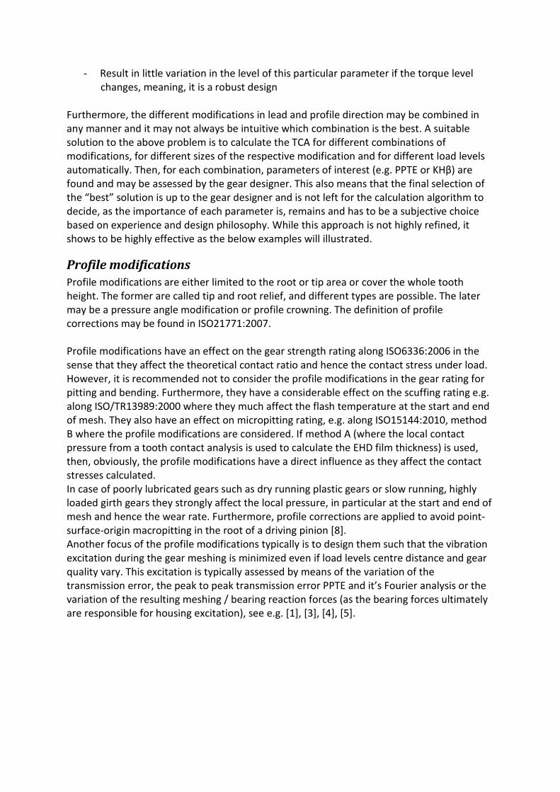
The resulting wear on the flank of one of the gears in the gear mesh before and after
optimization is shown in the next figure. It can be seen that by applying a combined
correction, the total wear can be reduced to about half of the original value, effectively
doubling the gear lifetime at no additional manufacturing cost.
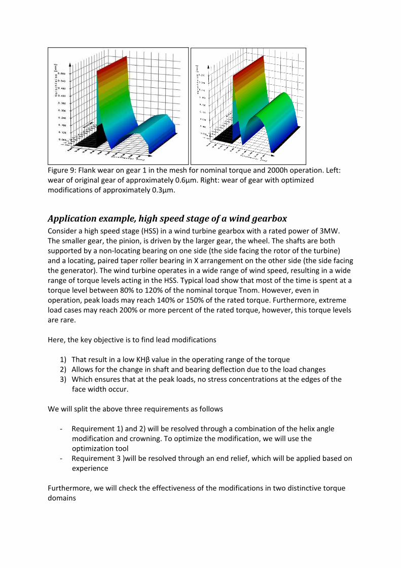
Figure 9: Flank wear on gear 1 in the mesh for nominal torque and 2000h operation. Left:
wear of original gear of approximately 0.6μm. Right: wear of gear with optimized
modifications of approximately 0.3μm.
Application example, high speed stage of a wind gearbox
Consider a high speed stage (HSS) in a wind turbine gearbox with a rated power of 3MW.
The smaller gear, the pinion, is driven by the larger gear, the wheel. The shafts are both
supported by a non-locating bearing on one side (the side facing the rotor of the turbine)
and a locating, paired taper roller bearing in X arrangement on the other side (the side facing
the generator). The wind turbine operates in a wide range of wind speed, resulting in a wide
range of torque levels acting in the HSS. Typical load show that most of the time is spent at a
torque level between 80% to 120% of the nominal torque Tnom. However, even in
operation, peak loads may reach 140% or 150% of the rated torque. Furthermore, extreme
load cases may reach 200% or more percent of the rated torque, however, this torque levels
are rare.
Here, the key objective is to find lead modifications
1) That result in a low KHβ value in the operating range of the torque
2) Allows for the change in shaft and bearing deflection due to the load changes
3) Which ensures that at the peak loads, no stress concentrations at the edges of the
face width occur.
We will split the above three requirements as follows
- Requirement 1) and 2) will be resolved through a combination of the helix angle
modification and crowning. To optimize the modification, we will use the
optimization tool
- Requirement 3 )will be resolved through an end relief, which will be applied based on
experience
Furthermore, we will check the effectiveness of the modifications in two distinctive torque
domains
- Torque domain A: operating load range, from 80% to 150% nominal torque. Here, we
want to achieve a low KHβ value and a good stress distribution.
- Torque domain B: extreme load range, at 200% nominal torque. Here, we want to
ensure that there are no stress concentrations at the end of the face width.
For the purpose of this study, we will put all modifications on the pinion and none on the
wheel and we will assume that the face width of both gears is equal. The deformation of the
bearings due to the gear forces is based on a non-linear bearing stiffness which is calculated
from the bearing inner geometry. The bearing stiffness is non-linear due to two effects
1) There is a finite bearing clearance which results in a horizontal line in the
displacement-force curve. This finite bearing clearance is calculated from the
assembly clearance (here, for the CRB, C3), the fit between the races and the shaft
and housing, the temperature of the bearing races and the centrifugal forces on the
races.
2) With increasing load, more rolling elements get into contact, effectively increasing
the stiffness with increasing load
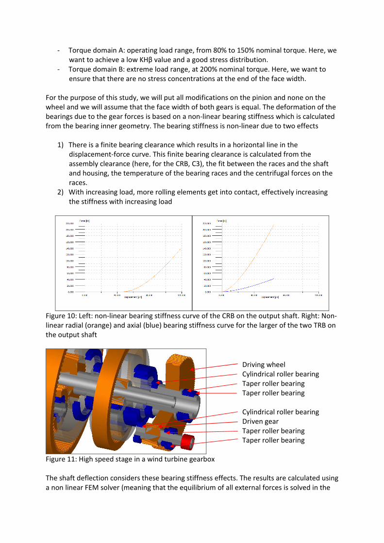
Figure 10: Left: non-linear bearing stiffness curve of the CRB on the output shaft. Right: Non-
linear radial (orange) and axial (blue) bearing stiffness curve for the larger of the two TRB on
the output shaft
Figure 11: High speed stage in a wind turbine gearbox
The shaft deflection considers these bearing stiffness effects. The results are calculated using
a non linear FEM solver (meaning that the equilibrium of all external forces is solved in the
Driving wheel
Cylindrical roller bearing
Taper roller bearing
Taper roller bearing
Cylindrical roller bearing
Driven gear
Taper roller bearing
Taper roller bearing

deformed state of the shaft), considering the shaft by means of Timoshenko type beam
elements and considering the bearings by means of a non linear spring / gap element.
Figure 12: Deformations in xy (orange) and zy (blue) plane. Left: Shaft deformation with C0
assembly clearance in the CRB. Right: Shaft deformation without clearance in the CRB.
Considering nominal torque and without any modifications, we find a contact stress
distribution as shown below, left side. Using the shaft calculation, we find an approximate
value for the helix angle modification Cβ=80μm and from experience, we estimate a suitable
crowning of Cb=20 μm and find a contact stress distribution as shown below, right side. We
can see that the contact pattern has improved but is not optimized. Furthermore, only
nominal load condition (100% of nominal torque) has been considered till now whereas in
wind gearboxes, a load level slightly higher than nominal torque should be considered in the
design of the gears.
Figure 13: Contact stress for nominal torque in plane of contact, without gear modifications.
Top left: No gear misalignment. Top right: With gear misalignment.
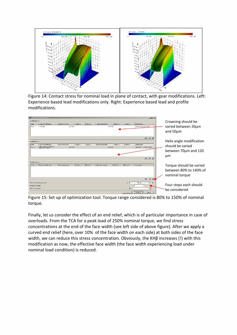
Figure 14: Contact stress for nominal load in plane of contact, with gear modifications. Left:
Experience based lead modifications only. Right: Experience based lead and profile
modifications.
Figure 15: Set up of optimization tool. Torque range considered is 80% to 150% of nominal
torque.
Finally, let us consider the effect of an end relief, which is of particular importance in case of
overloads. From the TCA for a peak load of 250% nominal torque, we find stress
concentrations at the end of the face width (see left side of above figure). After we apply a
curved end relief (here, over 10% of the face width on each side) at both sides of the face
width, we can reduce this stress concentration. Obviously, the KHβ increases (!) with this
modification as now, the effective face width (the face width experiencing load under
nominal load condition) is reduced.
Crowning should be
varied between 20μm
and 50μm
Helix angle modification
should be varied
between 70μm and 120
μm
Torque should be varied
between 80% to 140% of
nominal torque
Four steps each should
be considered

Figure 16: Contact stress in plane of contact for 250% nominal torque. Left: Stress
concentration at the end of the face width. Right: No stress concentration at the end of the
face width after an end relief has been applied.
Application example, sun-planet mesh in a mill gearbox
Horizontal (e.g. for sugar mills) or vertical (e.g. for cement mills) output planetary stages
transmit very high power levels at very low speed, resulting in large planetary stages having
with ratios d/b>1.00 – in particular on the sun gear. Due to the torsional wind up of the
planet carrier and the sun shaft, corrections in the sun-planet mesh are applied, the basic
considerations are explained e.g. in [14] or [15]. Care has to be taken not to select to high
levels of crowning, as the resulting loss in load carrying face width is severe. The design
objective is hence to find a combination of helix angle correction and crowning resulting in a
low KHβ value for different planet pin deflections and sun gear torsion, an objective that has
been reportedly achieved in the industry [13]. In this example, a gear face width of
b=430mm was applicable and the helix angle and the crowning on the sun gear were
selected as variables (while an end relief on the planet, having somewhat lower face width,
was applied).
The load level was varied in five steps between 90% and 130% of nominal load.
The crowning was varied between 10µm and 50µm and the helix angle modification
between -150µm and -190µm, both in five steps, giving a total of 125 calculations (25
different combinations of modifications, each for five different load levels). The result of
these are shown in the below graphics:

Figure 17: Resulting KHβ values for different load levels and different corrections
It can be seen that for modification 3:2:-, the lowest KHβ values result and that there, the
variation of the KHβ value is also small (KHβ is not much affected by the load level). For this
correction, the crowning is 30μm and the helix angle correction is -170μm.
Figure 18: Left: Lead corrections on planet gear. Right: Lead corrections on sun gear (lead
corrections in ring gear are not shown).

If we now look at the tooth contact pattern, the contact stress and KHβ for different load
levels (nominal load, lowest load and highest load) with the above corrections applied, we
find that
- KHβ (not considering manufacturing errors fma and fHβ) is low for all load cases
- KHβ varies only very little with the variation of the external loads
- For no load conditions, stress concentrations at the edge of the face width exists (also
due to the end relief)
We may therefore conclude that the design is robust, see the below images for the results at
lowest, nominal and highest load!
For 100% load and 240μm tilt
For the face load distribution factor KHβ we find:
KHβ =wmax/wm=2097N/mm/1980N/mm=1.06
For the contact stress in the plane of contact and the contact pattern on the sun we find:
Figure 19: Contact stress in plane of contact and contact pattern on sun gear for nominal
load.
For 90% load and scaled tilt, as lowest load
For the face load distribution factor KHβ we find:
KHβ =wmax/wm=1920N/mm/1782N/mm=1.08
For the contact stress in the plane of contact and the contact pattern on the sun we find:

Figure 20: Contact stress in plane of contact and contact pattern on sun gear for lowest load.
For 130% load and scaled tilt, as highest load
For the face load distribution factor KHβ we find:
KHβ =wmax/wm=2861N/mm/2574N/mm=1.11
For the contact stress in the plane of contact and the contact pattern on the sun we find:
Figure 21: Contact stress in plane of contact and contact pattern on sun gear for highest
load.
Summary
In the above four examples, general guidelines on the use and purpose of profile and lead
modifications have been presented. It is pointed out that the key to a successful design is
not only to optimize the modifications for a certain load level, but to take into account a
range of operating loads and selected overloads. While for overload cases, experience based
application of gear modifications makes sense, a search algorithm to find a robust
modification design for the whole range of operating loads is proposed.
We consider it critical that such an algorithm does not propose a single solution claiming it is
the best, but that the algorithm presents all solutions found for the designer to assess, e.g.
using graphics as shown above. While such an assessment could be automatic based on the
numerical results and user defined weights for each parameter, we strongly believe that
gear design is, remains and should be also intuitive. Above, a search algorithm, suitable

graphics for this intuitive assessment of the results and the application of the method in
various industries for different optimization targets are presented.
References
[1] Kissling, Effects of Profile Corrections on Peak-to-Peak Transmission Error, Gear
Technology, July 2010
[2] Houser, Hariant, Ueda, Determining the source of gear noise, Gear Solutions,
February 2004
[3] Houser, Harianto, Profile Relief and Noise Excitation in Helical Gears
[4] Palmer, Fish, Evaluation of Methods for Calculating Effects of Tip Relief on
Transmission Error, Noise and Stress in Loaded Spur Gears, Gear Technology,
January/February 2012
[5] Oswald, Townsend, Influence of Tooth Profile Modification on Spur Gear Dynamic
Tooth Strain, NASA Technical Memorandum 106952
[6] Kissling, Raabe, Calculating Tooth Form Transmission Error, Gear Solutions,
September 2006
[7] KISSsoft 03-2012
[8] Errichello, Hewette, Eckert, Point-Surface-Origin Macropitting Caused by Geometric
Stress Concentration
[9] Beermann, Estimation of lifetime for plastic gears, to be published
[10] KISSsoft AG, Wear on plastic gears, not published
[11] Venkatesan, Rameshkumar, Sivakumar, Simulation of Wear for High-Contact-
Ratio-Gear, Gear Technology India, April-June 2012
[12] Feulner, Verschleiss trocken laufender Kunststoffgetriebe, Lehrstuhl
Kunststofftechnik, Erlangen, 2008.
[13] Hess, Entwicklungstendenzen bei grossen Planetengetrieben für den
industriellen Einsatz, DMK2005
[14] MAAG Taschenbuch, 2nd Edition
[15] Amendola, Amendola, Yatzook, Longitudinal Tooth Contact Pattern Shift, Gear
Technology, May 2012