Algebraic Structures for Capturing the Provenance of ...
64
HAL Id: hal-01411827 https://hal.inria.fr/hal-01411827 Submitted on 7 Dec 2016 HAL is a multi-disciplinary open access archive for the deposit and dissemination of sci- entific research documents, whether they are pub- lished or not. The documents may come from teaching and research institutions in France or abroad, or from public or private research centers. L’archive ouverte pluridisciplinaire HAL, est destinée au dépôt et à la diffusion de documents scientifiques de niveau recherche, publiés ou non, émanant des établissements d’enseignement et de recherche français ou étrangers, des laboratoires publics ou privés. Copyright Algebraic Structures for Capturing the Provenance of SPARQL Queries Floris Geerts, Thomas Unger, Grigoris Karvounarakis, Irini Fundulaki, Vassilis Christophides To cite this version: Floris Geerts, Thomas Unger, Grigoris Karvounarakis, Irini Fundulaki, Vassilis Christophides. Alge- braic Structures for Capturing the Provenance of SPARQL Queries. Journal of the ACM (JACM), Association for Computing Machinery, 2016, 63 (1), pp.7. 10.1145/2810037. hal-01411827
Transcript of Algebraic Structures for Capturing the Provenance of ...

HAL Id: hal-01411827https://hal.inria.fr/hal-01411827
Submitted on 7 Dec 2016
HAL is a multi-disciplinary open accessarchive for the deposit and dissemination of sci-entific research documents, whether they are pub-lished or not. The documents may come fromteaching and research institutions in France orabroad, or from public or private research centers.
L’archive ouverte pluridisciplinaire HAL, estdestinée au dépôt et à la diffusion de documentsscientifiques de niveau recherche, publiés ou non,émanant des établissements d’enseignement et derecherche français ou étrangers, des laboratoirespublics ou privés.
Copyright
Algebraic Structures for Capturing the Provenance ofSPARQL Queries
Floris Geerts, Thomas Unger, Grigoris Karvounarakis, Irini Fundulaki,Vassilis Christophides
To cite this version:Floris Geerts, Thomas Unger, Grigoris Karvounarakis, Irini Fundulaki, Vassilis Christophides. Alge-braic Structures for Capturing the Provenance of SPARQL Queries. Journal of the ACM (JACM),Association for Computing Machinery, 2016, 63 (1), pp.7. �10.1145/2810037�. �hal-01411827�

7
Algebraic Structures for Capturing the Provenanceof SPARQL Queries
FLORIS GEERTS, University of AntwerpTHOMAS UNGER, University College DublinGRIGORIS KARVOUNARAKIS, LogicBloxIRINI FUNDULAKI, ICS-FORTHVASSILIS CHRISTOPHIDES, Inria Paris-Rocquencourt
The evaluation of SPARQL algebra queries on various kinds of annotated RDF graphs can be seen as aparticular case of the evaluation of these queries on RDF graphs annotated with elements of so-calledspm-semirings. Spm-semirings extend semirings, used for representing the provenance of positive relationalalgebra queries on annotated relational data, with a new operator to capture the semantics of the non-monotone SPARQL operators. Furthermore, spm-semiring-based annotations ensure that desired SPARQLquery equivalences hold when querying annotated RDF. In this work, in addition to introducing spm-semirings, we study their properties and provide an alternative characterization of these structures in termsof semirings with an embedded boolean algebra (or seba-structure for short). This characterization allowsus to construct spm-semirings and identify a universal object in the class of spm-semirings. Finally, we showthat this universal object provides a provenance representation of poly-sized overhead and can be used toevaluate SPARQL queries on arbitrary spm-semiring-annotated RDF graphs.
CCS Concepts: � Information systems → Data provenance; Query languages for non-relationalengines
Additional Key Words and Phrases: Algebraic structures, annotations, provenance models, query languages,RDF, SPARQL
ACM Reference Format:Floris Geerts, Thomas Unger, Grigoris Karvounarakis, Irini Fundulaki, and Vassilis Christophides. 2016.Algebraic structures for capturing the provenance of SPARQL queries. J. ACM 63, 1, Article 7 (February2016), 63 pages.DOI: http://dx.doi.org/10.1145/2810037
1. INTRODUCTION
The W3C Linked Data Initiative has boosted the publication and interlinkage of mas-sive amounts of scientific, corporate, governmental, and crowd-sourced datasets on theemerging Data Web. These data are commonly published in the form of RDF data[Manola et al. 2004] and queried with the SPARQL query language [Prud’hommeaux
Authors’ addresses: F. Geerts, Department of Mathematics & Computer Science, University of Antwerp,Middelheimlaan 1, 2020 Antwerp, Belgium; email: [email protected]; T. Unger, School of Math-ematics and Statistics, University College Dublin, Belfield, Dublin 4, Ireland; email: [email protected];G. Karvounarakis, LogicBlox, 1349 West Peachtree Street NW, Suite 1880, Atlanta, GA 30309, USA; email:[email protected]; I. Fundulaki, Institute of Computer Science (ICS), Foundation for Re-search and Technology-Hellas (FORTH), N. Plastira 100, Vasilika Vouton, Heraklion, Greece, 70013; email:[email protected]; V. Christophides, Inria Paris-Rocquencourt. Laboratory of Information, Networking andCommunication Sciences, 23 avenue d’Italie, 75013 Paris, France; email: [email protected] to make digital or hard copies of part or all of this work for personal or classroom use is grantedwithout fee provided that copies are not made or distributed for profit or commercial advantage and thatcopies show this notice on the first page or initial screen of a display along with the full citation. Copyrights forcomponents of this work owned by others than ACM must be honored. Abstracting with credit is permitted.To copy otherwise, to republish, to post on servers, to redistribute to lists, or to use any component of thiswork in other works requires prior specific permission and/or a fee. Permissions may be requested fromPublications Dept., ACM, Inc., 2 Penn Plaza, Suite 701, New York, NY 10121-0701 USA, fax +1 (212)869-0481, or [email protected]© 2016 ACM 0004-5411/2016/02-ART7 $15.00DOI: http://dx.doi.org/10.1145/2810037
Journal of the ACM, Vol. 63, No. 1, Article 7, Publication date: February 2016.
7:2 F. Geerts et al.
and Seaborne 2008]. In such settings where RDF data are freely exchanged, integrated,and materialized in distributed repositories, it is crucial to be able to assess the qualityof replicated and possibly incomplete or uncertain data.
Toward this end, several models for annotated RDF data have been proposed [Carrollet al. 2005; Mazzieri and Dragoni 2008; Hartig 2009; Dividino et al. 2009; Huangand Liu 2009; Zimmermann et al. 2012; Straccia 2013] in an attempt to representvarious dimensions of data quality such as trust, truth of imprecise information, orthe probability of the validity of the data. In all these cases, when annotated data aretransformed through SPARQL queries, one needs to compute appropriate annotationsfor the query results. For instance, in the case of trust assessment [Hartig 2008, 2009;Dividino et al. 2009], the trustworthiness of query results is determined based onthe trustworthiness of source datasets from which they were derived. Similarly, foruncertain and fuzzy datasets, the degrees of truth of query results are derived basedon the degrees of truth associated with the original data [Dividino et al. 2009; Huangand Liu 2009; Zimmermann et al. 2012; Straccia 2013].
If we are only interested in one kind of annotations, and source annotations arestatic and common for all users as well as available at query evaluation time, suchcomputations can be performed during query evaluation [Hartig 2008, 2009; Dividinoet al. 2009; Huang and Liu 2009; Zimmermann et al. 2012; Straccia 2013].
In general however, various different scenarios may present themselves: Differentapplications may require computing different kinds of annotations over the same sourcedata and queries; for a single kind of annotation (especially in data integration andwarehouse settings) data may be collected from various RDF sources that changeover time; different users may have different beliefs about aspects of the data andthese beliefs may not be available at query evaluation time or may change over time;different users may only be interested in computing annotations for a small subset ofthe results of a query, and the like.
As a consequence, we may end up with redundant query evaluations. The samequery may have to be evaluated repeatedly over the same source data for each kindof annotation. Even if source annotations representing the beliefs of each user areavailable at query evaluation time, the same query may have to be evaluated separatelyfor each one of these sets of source annotations despite the fact that the relationship ofquery results with the source data is the same for all users. Because we do not knowin advance which query results will be derived, or which subset of the source data isinvolved in their derivation, annotations for all results of each query may need to becomputed during query evaluation.
For these reasons, abstract provenance models [Green et al. 2007] have been intro-duced: They use abstract tokens to represent tuple annotations and abstract operatorsto capture the relationship between the query operators that combine source datato derive query results. Conceptually, the resulting abstract provenance expressionsencode for each query result its relationship to source data and query operators, asimplied by the structure of the query, independently of any specific kind of annotationsor particular source data annotation values. Such expressions can then be computedonce during query evaluation, and annotations for various applications or users withdifferent beliefs or specific query results can be computed from them, without requiringredundant re-evaluation(s) of each query over all source data.
In the relational setting, provenance models that are capable of abstracting thequery evaluation on annotated relational data have been put forward for the positivefragment of the relational algebra [Cheney et al. 2009]. In particular, the modelingof annotations by means of semirings has shown great promise [Green et al. 2007],both as a platform for theoretical study and as a representation employed in systemsthat record provenance information when data are imported in the hosting repository
Journal of the ACM, Vol. 63, No. 1, Article 7, Publication date: February 2016.

Algebraic Structures for Capturing the Provenance of SPARQL Queries 7:3
[Karvounarakis et al. 2013] and use it to compute appropriate annotations for differentapplications and users at a later time [Karvounarakis et al. 2010].
For annotated RDF data and positive SPARQL queries (those that use only the ANDand UNION operators), one can verify, similarly to the positive relational case, thatsemirings suffice as the annotation structure [Theoharis et al. 2011]. However, whenthe non-monotone SPARQL operator OPTIONAL is brought into the picture, it can easilybe verified that extensions of semirings have to be considered. Indeed, the SPARQL 1.0algebra semantics [Perez et al. 2009] of OPTIONAL is defined in terms of a left-outer jointhat involves a non-monotone difference algebraic operator. More specifically, for anytwo RDF data sets G1 and G2, (G1 OPTIONAL G2) can be written as (G1 AND G2) UNION(G1 DIFFERENCE G2) [Perez et al. 2009]. Although DIFFERENCE is—strictly speaking—notpart of the SPARQL 1.0 specification, we add it for convenience.1
However, as explained in Section 2, the semantics of DIFFERENCE and OPTIONAL arenot the same as those of relational difference and (left-)outer join, respectively. Thus,extensions to the semiring framework intended to cope with the latter [Geerts andPoggi 2010; Amsterdamer et al. 2011a, 2011b; Glavic and Alonso 2009] cannot beapplied directly to capture the provenance of SPARQL queries. Recent work [Damasioet al. 2012] suggests that it may be possible to express the SPARQL difference interms of relational operators to leverage the structure of m-semirings, an extension ofsemirings for relational queries involving difference [Geerts and Poggi 2010]. However,whereas a provenance model based on the so-called universal m-semiring exists, thismodel does not allow for a concise and simple representation of its expressions [Geertsand Poggi 2010] and, thus, its practical usability as a provenance model is ratherlimited.
For these reasons, we propose a new algebraic structure for capturing the semanticsof SPARQL DIFFERENCE (and thus also OPTIONAL) in this article. More specifically, weidentify a set of SPARQL query equivalences that involve DIFFERENCE and hold underboth bag and set semantics, and we show that these equivalences also hold whenevaluating SPARQL queries on a wide variety of annotated RDF data. Then, we defineso-called spm-semirings, an extension of semirings with a new operation �, basedon identities derived from the aforementioned SPARQL equivalences. Furthermore,we show that spm-semirings do have a universal structure that provides a conciserepresentation of the provenance of RDF data and SPARQL queries involved.
The underlying techniques rely on a characterization of spm-semirings in terms ofsemirings with an embedded boolean algebra, or seba-structure for short. This char-acterization is nontrivial and may be of interest in its own right. Furthermore, thespm-semiring-based provenance expressions can indeed be used to compute appropri-ate annotations in a wide variety of application domains. We thus provide a completepicture of SPARQL query evaluation on annotated RDF and propose an abstract prove-nance model that incorporates non-monotone SPARQL operators. We note that therelational analogue is still open for relational queries with difference.
In summary, we make the following contributions:
(1) We illustrate that the semantics of SPARQL on various notions of annotated RDFhave a great commonality (Section 2). Based on this, we generalize the semanticsof SPARQL algebra expressions to RDF data annotated with values from somearbitrary annotation domain K, or K-annotated RDF for short (Section 3). For thispurpose, K is equipped with binary operations ⊕, ⊗, and �, and constants 0 and 1that accommodate all SPARQL algebra operators.
1The algebra described in the SPARQL 1.1 specification [Harris and Seaborne 2013] also contains a similaroperator called MINUS. We discuss SPARQL 1.1 in Section 8.
Journal of the ACM, Vol. 63, No. 1, Article 7, Publication date: February 2016.

7:4 F. Geerts et al.
(2) We identify a set of SPARQL algebra equivalences (some involving DIFFERENCE)that are desirable to hold on K-annotated RDF (Section 4). We show that for theseequivalences to hold, (K,⊕,⊗,�, 0, 1) must be an spm-semiring and vice versa. Aminimal set of identities defining spm-semirings is provided.
(3) An alternative characterization of spm-semirings is given in Section 5, based onsemirings with an embedded boolean algebra (seba-structures). We prove the cor-rectness of this characterization and show how it can be used to construct spm-semirings based on semirings commonly used in practice.
(4) We identify a universal object in the class of spm-semirings (Section 6), leveragingthe characterization in terms of seba-structures, and show that the evaluation ofSPARQL queries on spm-semiring annotated RDF factors through the evaluationof RDF annotated with elements in the universal object. The universal object istherefore proposed in Section 7 as a provenance model for annotated RDF andSPARQL. Furthermore, we explain how newly introduced non-monotone operatorsin SPARQL 1.1 fit into our algebraic framework in Section 8. Finally, we comparespm-semirings with related work in the relational and semantic Web contexts inSection 9 and conclude with directions for future work in Section 10.
This article is a considerable expansion of the 12-page conference paper [Geerts et al.2013]. Apart from providing all definitions and proofs, we have included ample ex-amples illustrating key concepts. Furthermore, we have corrected several mistakes,especially those concerning the construction of the universal objects.
2. QUERYING ANNOTATED RDF
In this section, we provide examples of the evaluation of SPARQL queries on annotatedRDF data. We first recall RDF [Manola et al. 2004] and SPARQL [Prud’hommeaux andSeaborne 2008] with the standard bag semantics in which we represent multiplicitiesas annotations. We then observe that, similar to the relational case, the semantics ofSPARQL on various forms of annotated RDF have a great commonality.
2.1. RDF and SPARQL in a Nutshell
RDF is the standard model for representing semantic Web data as sets of triples ofthe form (subject, predicate, object). Intuitively, for each triple, the predicate describesthe relationship between subject and object. For instance, Table (a) of Figure 1 showsan example of an RDF triple set, denoted by G, where the columns stand for thecorresponding components of each triple (S for subject, P for predicate, and O forobject). SPARQL is the standard language used to query RDF data. We present theSPARQL semantics based on the algebra of Perez et al. [2009]. The operators of thisalgebra manipulate bags of mappings (i.e., valuations of variables to constants in G)and include unary operators σ and π that correspond to the SPARQL constructs FILTERand SELECT, respectively, and binary operators ∪, �, and � for the SPARQL constructsUNION, AND, and OPTIONAL, respectively. The operator � can be defined in terms of ∪,�, and \, the algebraic counterpart of DIFFERENCE [Perez et al. 2009]. The followingexample illustrates the standard bag semantics of SPARQL queries.
Example 2.1 (bags). In Figure 1 we start by considering the simplest SPARQL query(?x, ?y, ?z) over the RDF triple set G depicted in Table (a). Such a query is referred toas a triple pattern where ?x, ?y, and ?z denote variables. Intuitively, the evaluation ofthe triple pattern (?x, ?y, ?z) consists of a bag of mappings. Each mapping correspondsto the selection of a triple from the RDF triple set G by bounding the variables toconstants in triples in G. Table (b) shows the resulting mapping bag �. We employ
Journal of the ACM, Vol. 63, No. 1, Article 7, Publication date: February 2016.

Algebraic Structures for Capturing the Provenance of SPARQL Queries 7:5
Fig. 1. Example of RDF graph and evaluation of SPARQL algebra operators (bag/trust/fuzzy semantics).
symbol μi to identify individual mappings. The formal definition of triple patterns andgeneral SPARQL queries is provided at the beginning of Section 3.
To simplify the presentation, we use the tabular representation of the mapping bagsshown in Table (b) in Figure 1, where the first three columns correspond to variablesin the mappings and the fourth column (#) represents the multiplicity of the mapping.The last two columns (trust and fuzzy ) can be ignored for now, as can the gray shadedentries in Tables (h) and (i).
Tables (c–e) illustrate the evaluation of the operators σ and π . The output mappingbags are denoted by �1, �2, and �3. For instance, mapping μ11 of �3 has two derivationsoriginating from mappings in �; namely, one by projecting μ4 and another one byprojecting μ5. The multiplicity of μ11 is obtained by adding the multiplicities of μ4 andμ5.
Table (f) shows the result of �4 = �2 ∪ �3, where �2 and �3 are shown in Tables(d) and (e), respectively. In �4, the mapping μ13 has two derivations, both of themoriginating from �3, whereas the two derivations of μ12 originate from �2 (μ8) and �3(μ10). The multiplicity of μ12 is obtained by adding the multiplicities of μ8 and μ10.
Table (g) depicts the result of �4 � �1. For instance, mapping μ16 is derived by joiningμ13 ∈ �4 and μ6 ∈ �1. Mappings can be joined only if they are compatible [Perez et al.2009]. In our example, μ6 and μ13 are compatible because they agree on their commonvariable (i.e., they both bind ?y to b). The multiplicity of μ16 is computed as the productof the multiplicities of the two input mappings (1 × 2 = 2).
Table (h) illustrates an example of the difference operator (i.e., �4 \ �1). Note thatneither μ12 nor μ13 in �4 are in the result—recall that we ignore the gray-shaded entriesfor now—because �1 contains a mapping (μ6) that is compatible with the mappingsμ12 and μ13 in �4 as explained earlier. On the other hand, there is no mapping in
Journal of the ACM, Vol. 63, No. 1, Article 7, Publication date: February 2016.

7:6 F. Geerts et al.
�1 that is compatible with μ14. As a consequence, μ14 appears in the result as μ19 inTable (h). Note that the difference operator can be applied on bags of mappings definedon different variables since only the common variables of the mappings are considered.This is also true for the SPARQL union.
Finally, Table (i) depicts the result of �4 � �1, which contains all mappings fromTables (g) and (h). Indeed, �4 � �1 = (�4 � �1) ∪ (�4 \ �1). The symbol “−” denotesthat ?x is not bound to a constant in the mappings μ22, μ23 and μ24.
The previous example shows that the multiplicities of mappings in the result of σ , π ,∪, and � SPARQL algebra operators are computed in a similar way as when evaluatingthe corresponding operators of the relational algebra under bag semantics [Green et al.2007]. In particular, in the case of alternative derivations (e.g., for π or ∪) of a mapping,its multiplicity equals the sum of the multiplicities of the different derivations. In thecase of �, the multiplicity of the result mapping equals the product of the multiplicitiesof the two input mappings that were combined.
However, the multiplicities of the result mappings of the \ operator are computeddifferently from the corresponding case of the difference operator (\ra) in the rela-tional algebra under bag semantics. Indeed, let R and S be two relations and de-note by R(t) and S(t) the multiplicity of a tuple t in R and S, respectively. Then,(R \ra S)(t) := max(0, R(t) − S(t)) in the bag semantics of the relational algebra [Greenet al. 2007]. In contrast, the SPARQL difference (\) is defined in terms of compatibility,not equality [Schmidt et al. 2010]. Indeed, Table (h) shows that when considering theSPARQL difference �4 \�1, a mapping (tuple) t in �4 is in the output as long as there isno mapping in �1 that is compatible with it. That is, (�4 \�1)(t) = �4(t) −bag �t′∼t�1(t′),where for any two natural number n and m, n −bag m = n in case that m = 0, andn −bag m = 0 otherwise. Thus, SPARQL follows the standard relational bag semanticsfor its positive operators but uses a different semantics for \. Similarly, relational left-outer join, which is defined as a union between a join and a relational difference, alsouses a different semantics than SPARQL OPTIONAL.
Example 2.2 (bags cont’d). Consider Tables (c), (f), and (h) of Figure 1. Observe thatalthough μ12 and μ13 both have multiplicity 2 in �4 (Table (f)), and the compatiblemappings μ6 and μ7 in �1 have multiplicity 1 (Table (c)), neither μ12 nor μ13 is presentin �4 \ �1. As another example, consider π?y(�1) consisting of mappings μ′
6 and μ′7
obtained as the projection on the variable ?y of μ6 and μ7 in �1, respectively. Thesemappings both have multiplicity 1. Furthermore, consider π?y(�4) consisting of map-pings μ′
12+13 and μ′14 obtained as the projection on the variable ?y of μ12 and μ13, and
μ14 in �4, respectively. The mapping μ′12+13 has multiplicity 4 and the mapping μ′
14 hasmultiplicity 1. As before, when considering π?y(�4) \ π?y(�1), the mapping μ′
12+13 willnot be present in the result despite the fact that μ′
12+13 has a higher multiplicity thanμ′
6. Since the mapping bags π?y(�1) and π?y(�4) are defined over the same schema (with“attribute” ?y), we can also consider
(π?y(�4)
) \ra(π?y(�1)
). In this case, μ′
12+13 wouldbe in the result with multiplicity 3, as given by max(0, 4 − 1).
2.2. SPARQL on Annotated RDF
We next consider the semantics of SPARQL when RDF is adorned with trust informa-tion [Hartig 2008, 2009; Dividino et al. 2009]. In this setting, for a given SPARQL query,the goal is to find which result mappings are trusted based on the trustworthiness ofthe input mappings. More specifically, in case of mappings with multiple derivations,a single trusted derivation suffices to infer that the result mapping is trusted. Whentwo mappings are combined in a derivation, both of them should be trusted in orderfor the result mapping to be trusted. Based on this semantics, which has also been
Journal of the ACM, Vol. 63, No. 1, Article 7, Publication date: February 2016.

Algebraic Structures for Capturing the Provenance of SPARQL Queries 7:7
studied in the relational context [Karvounarakis et al. 2013; Green et al. 2007], onecan compute the trusted result mappings by answering the query over the subset ofthe input consisting of trusted triples only. This semantics also coincides with the setsemantics of SPARQL [Perez et al. 2009] in which a trusted mapping belongs to theoutput mapping set and an untrusted mapping does not.
Example 2.3 (trust, set). Consider Figure 1 where, instead of the # column, we nowfocus on the annotations in the trust column. For example, each triple in Table (b)comes with a boolean trust value (τi) that is true if the triple is trusted and falseotherwise. It is readily verified that the desired trust semantics is obtained for theexample SPARQL queries in Figure 1 by combining trust values through disjunction(∨) and conjunction (∧), instead of addition and multiplication, respectively, used tocompute multiplicities in Example 2.1. For example, μ11 in Table (e) is trusted only ifone of the mappings μ4 or μ5 is trusted. Similarly, μ16 in Table (g) is trusted if μ1 istrusted and either μ4 or μ5 is trusted. To deal with \, we consider boolean negation(denoted by τ for a trust variable τ ). Indeed, consider the gray-shaded entry μ18 inTable (h). This mapping is trusted only if μ1 is untrusted and either μ4 or μ5 is trusted.This is expressed by (τ4 ∨ τ5) ∧ τ1 and denoted by (τ4 ∨ τ5) −trust τ1 in Table (h). Hence,the gray-shaded mappings can be part of the result depending on the trust informationof the source mappings. In general, if ϕ and ψ are two propositional formulas overboolean variables, then their difference is defined as ϕ −trustψ := ϕ ∧ ψ . Note that thisis similar to the notion of difference given in the bag semantics (cf. Example 2.1): ϕ ∧ ψequals ϕ if ψ is false, and equals false otherwise.
We conclude this section by considering SPARQL on fuzzy RDF data [Zimmermannet al. 2012; Straccia 2013]. In this setting, every mapping is annotated with a realnumber in the range [0, 1], where the annotation denotes the degree of truth that themapping exists in the particular mapping set. Mappings annotated with 0 certainly donot exist in the mapping set, whereas those annotated with 1 certainly exist. In thecase of mappings with alternative derivations, the degree of truth of the mapping isthat of the derivation with the highest degree of truth while the degree of truth of acomposite derivation equals the minimum of the degrees of truth over the two inputmappings.
Example 2.4 (fuzzy). Consider Figure 1 where instead of the # column, we now focuson the fuzzy column. For example, each triple in Table (b) comes with a degree of truth(pi) that is a real number in [0, 1]. It is readily verified that the desired fuzzy semanticsis obtained for the example SPARQL queries in Figure 1 if we take the maximum (max)and minimum (min) instead of addition and multiplication, respectively, as used forbag semantics (cf. Example 2.1). To deal with \, we need to consider an additionaloperator −fuzzy on degrees of truth that is defined as p −fuzzy q := p in case that q =0, and p −fuzzy q := 0 otherwise. This definition is in line with the treatment of theOPTIONAL operator in the fuzzy RDF setting [Zimmermann et al. 2012; Straccia 2013].For example, the gray-shaded entry μ18 in Table (h) appears with degree of truthmax(p4, p5)−fuzzy p1. That is, if μ1 has non-zero degree of truth, then μ18 will not appearin the query result. Similarly, if both p4 and p5 have zero degree of truth, then μ18 isnot part of the output. In all other cases, μ18 is a result mapping with degree of truthmax(p4, p5). Note again the similarity between −fuzzy, −bag and −trust.
We remark that Dividino et al. [2009] define p −fuzzy q as min(p, 1 − q). Althoughthis definition collapses to −trust when p and q can only be 0 or 1, it is not compatiblewith the standard bag semantics. Instead, we aim to provide a general treatment thatcovers the SPARQL semantics in the setting of sets and bags and beyond. Furthermore,
Journal of the ACM, Vol. 63, No. 1, Article 7, Publication date: February 2016.

7:8 F. Geerts et al.
defining p −fuzzy q as in Dividino et al. [2009] does lead to a semantics of SPARQL forwhich desired query equivalences (introduced in the next section) are not satisfied. Wetherefore adopt the fuzzy semantics given by Zimmermann et al. [2012] and Straccia[2013].
2.3. Summary and Lookahead
The previous examples suggest a commonality between the different semantics ofSPARQL on annotated RDF. Similar to the semiring-based approach for annotatedrelational data, we unify the semantics of SPARQL for a wide range of annotations asfollows: First, we extend mappings to annotated mappings that take values in someabstract set K of annotations. Second, we enrich K with operations for capturing thesemantics of the query language operators. More specifically, we enrich K with thefollowing three binary operations:
—A binary operator ⊕ for modeling +, ∨, and max, among others, for the operators πand ∪;
—A binary operator ⊗ for modeling ×, ∧, and min, among others, for the operators �
and �; and—A binary operator � for modeling −bag, −trust, and −fuzzy, among others, for the
operators \ and �.
Finally, based on SPARQL query equivalences that are known to hold in the bag,trust (set), and fuzzy setting, among others, we identify a set of additional propertiesthat the algebraic structure consisting of K, ⊕, ⊗, and � must have, and we providea characterization of these structures. We provide additional examples of annotatedRDF commonly used in practice in Section 5 and show that these are all unified by ourapproach.
3. SEMANTICS OF SPARQL ON ANNOTATED RDF
In this section, we formalize the semantics of SPARQL on annotated RDF. We startby defining a general notion of annotated RDF and then extend the semantics ofSPARQL correspondingly. In this section, we consider SPARQL 1.0 [Prud’hommeauxand Seaborne 2008] and discuss SPARQL 1.1 in Section 8.
We would like to emphasize that we do not consider the deductive process of obtainingimplicitly entailed triples. We follow the official W3C SPARQL specification in whichthe semantics of SPARQL disregards the issue of RDFS reasoning. This means thatSPARQL operates on the RDF graph as is, without inferring new triples. Wheneverreasoning is desired, it is assumed to be carried out by a separate, underlying layer.This decision, which keeps the SPARQL query language independent from the reason-ing process, brings several advantages: It results in a clean and compact semanticsfor SPARQL that does not interfere with reasoning rules, makes the SPARQL querylanguage resistant to possible changes in the RDF(S) reasoning process, and allows theuse of SPARQL without modifications on top of other reasoning mechanisms.
Let I, B, and L be pairwise disjoint infinite sets of Internationalized Resource Iden-tifiers (IRIs), blank nodes, and literals, respectively. A triple (s, p, o) ∈ (I ∪ B) × I × (I ∪B ∪ L) is called an RDF triple. As mentioned earlier, s is the subject, p the predicate,and o the object. An RDF graph is a finite set of RDF triples.
Definition 3.1. Let K be a set of annotations, disjoint from I, B, and L. A K-annotatedRDF triple is of the form (s, p, o) �→ k where (s, p, o) is an RDF triple and k is an
Journal of the ACM, Vol. 63, No. 1, Article 7, Publication date: February 2016.

Algebraic Structures for Capturing the Provenance of SPARQL Queries 7:9
annotation taken from K. A finite set of annotated RDF triples is called a K-annotatedRDF graph if every triple (s, p, o) has a single annotation in K.2
Similarly to Perez et al. [2009], we consider a fragment of SPARQL consisting ofgraph pattern expressions, which are defined inductively as follows. Let V be a set ofvariables, disjoint from I, B and L.
(1) A triple from (I ∪ V ) × (I ∪ V ) × (I ∪ L∪ V ) is a graph pattern, referred to as a triplepattern.
(2) If P1 and P2 are graph patterns, then (P1 UNION P2), (P1 AND P2), and (P1 OPT P2)are also graph patterns, referred to as a union, conjunction, and optional graphpattern, respectively.
(3) If P is a graph pattern and R is a SPARQL built-in condition, then (P FILTER R)is a graph pattern, referred to as a filter graph pattern.
(4) If P is a graph pattern and S ⊆ V , then SELECTS(P) is a graph pattern, referredto as a projection graph pattern.
Here, a SPARQL built-in condition is constructed using elements of the set I ∪ L ∪ Vand constants, logical connectives (¬, ∧, ∨), inequality symbols (<, �, �, >), the equal-ity symbol (=), unary predicates like bound, isBlank, and isIRI, plus other features(see Harris and Seaborne [2013] for a complete list of built-in conditions).
We next extend the semantics of SPARQL from RDF graphs to K-annotated RDFgraphs, hereby closely following the presentation of the standard semantics of SPARQLgiven in Perez et al. [2009]. That is, in the standard, unannotated setting, the semanticsof SPARQL graph patterns on RDF graphs can be defined in terms of SPARQL algebraoperations on mapping sets. Later, we first generalize mapping sets to K-annotatedmapping sets, define the semantics of the SPARQL algebra operators on such mappingsets, and then extend the semantics of SPARQL in terms of the SPARQL algebraoperators. The algebra operators consist of union (∪), join (�), difference (\), left outerjoin ( �), projection (π ), and selection (σ ). We note that the difference operator is not aSPARQL operator; it was introduced by Perez et al. [2009] to specify the semantics ofthe left outer join operator [Harris and Seaborne 2013].
Let var (t) denote the set of variables from V that appear in a triple pattern t anddenote I ∪ B ∪ L by T . A mapping μ from V to T is a partial function μ : V → T .The domain of μ, denoted by dom (μ), is the subset of V on which μ is defined. Wesay that two mappings μ1 and μ2 are compatible if for all v ∈ dom (μ1) ∩ dom (μ2) wehave μ1(v) = μ2(v). We denote this by μ1 ∼ μ2. It is readily verified that if μ1 ∼ μ2,then μ1 ∪ μ2 is also a mapping from V → T . We denote by M the set of all mappingsfrom V to T . Note that empty mappings (mappings with empty domains) are alwayscompatible.
Definition 3.2. Let K be a set of annotations and let 0 denote a distinguished elementfrom K. A K-annotated mapping set on M is a total function � : M → K such that itssupport {μ ∈ M | �(μ) �= 0} is finite.
Intuitively, we interpret a mapping in M with its annotation set to 0 by � as notbeing part of the mapping set �. Definition 3.2 can thus be interpreted as saying thatmapping sets � consist of a finite number of mappings (i.e., only a finite number ofmappings have a non-zero annotation).
2Although the definition implies that a triple is associated with a single annotation, no generality is lost.Indeed, in application scenarios where triples may have multiple annotations from the same domain, it iscommon practice to combine these annotations [Zimmermann et al. 2012]. More specifically, (s, p, o) → k1and (s, p, o) → k2 is represented by (s, p, o) → k1 ⊕ k2.
Journal of the ACM, Vol. 63, No. 1, Article 7, Publication date: February 2016.
7:10 F. Geerts et al.
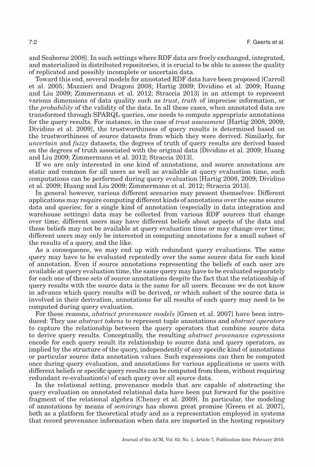
To generalize the SPARQL algebra operators to K-annotated mapping sets, we re-quire K to be equipped with binary operations ⊕, ⊗, and �; to contain two distinguishedconstants 0 and 1; and—for reasons that will be clear shortly—we assume that ⊕ and⊗ are commutative. The definitions below are inspired by the bag, trust (set), and fuzzysemantics of SPARQL, as illustrated in Section 2. The algebra operations on mappingsets are defined as follows. Let � be a K-annotated mapping set on M, S ⊆ V and let Rbe a SPARQL built-in condition. Then, for all μ ∈ M and ν ∈ M such that dom (ν) ⊆ S:
(σR(�))(μ) := �(μ) ⊗ FR(μ)
(πS(�))(ν) :=⊕
μ∈M,∃μ′∈Mμ=ν∪μ′&dom (μ′)∩S=∅
�(μ),
where, for all μ ∈ M, FR(μ) = 1, if μ satisfies the built-in condition R and FR(μ) = 0otherwise. We refer to Perez et al. [2009] for the definition of when a mapping satisfiesa built-in condition. Let �1 and �2 be two K-annotated mapping sets. Then, for allμ ∈ M:
(�1 ∪ �2)(μ) := �1(μ) ⊕ �2(μ)
(�1 � �2)(μ) :=⊕
μ1,μ2∈Mμ=μ1∪μ2
�1(μ1) ⊗ �2(μ2)
(�1 \ �2)(μ) := �1(μ) � ( ⊕μ′∈M,μ∼μ′
�2(μ′))
(�1 � �2)(μ) := ((�1 � �2) ∪ (�1 \ �2))(μ).
We refer to this as the SPARQL K-annotated algebra. The algebra operations onK-annotated mapping sets are well-defined (i.e., they are independent of the order inwhich mappings in M are considered). Indeed, the annotations associated with theoperations πS, �, \, and � involve the summation (using ⊕) and products (using ⊗) ofvalues in K corresponding to sets of compatible mappings. The resulting annotationsare independent of the order in which these compatible mappings are considered. Thisis a direct consequence of our assumption that ⊕ and ⊗ are commutative.
The semantics of our fragment of SPARQL on K-annotated RDF graphs is nowdefined inductively, following the definition of graph patterns, in terms of the SPARQLK-annotated algebra. That is, we first define the evaluation of a triple pattern t on aK-annotated RDF graph Ga as the following K-annotated mapping set. For all μ ∈ M:
[[t]]Ga(μ) :={
k if dom (μ) = var (t), μ(t) �→ k ∈ Ga0 otherwise.
Here, for a triple pattern t, we denote by μ(t) the triple obtained by replacing thevariables in t according to μ. Note that this is indeed a K-annotated mapping set:(i) it defines a function because RDF triples in Ga have a single annotation, and (ii) ithas finite support since RDF graphs are finite objects. The semantics of the remainingSPARQL graph patterns is defined as follows: Let P1 and P2 be graph patterns, R abuilt-in condition, and S ⊆ V . Then,
[[P1 FILTER R]]Ga := σR([[P1]]Ga
)[[SELECTS P1]]Ga := πS
([[P1]]Ga
)[[P1 UNION P2]]Ga := [[P1]]Ga ∪ [[P2]]Ga
[[P1 AND P2]]Ga := [[P1]]Ga � [[P2]]Ga
[[P1 OPT P2]]Ga := [[P1]]Ga � [[P2]]Ga .
Journal of the ACM, Vol. 63, No. 1, Article 7, Publication date: February 2016.

Algebraic Structures for Capturing the Provenance of SPARQL Queries 7:11
For convenience, we also consider a SPARQL graph pattern for the difference:
[[P1 DIFFERENCE P2]]Ga := [[P1]]Ga \ [[P2]]Ga .
This graph pattern is not part of the SPARQL syntax, but, from the relationshipbetween the SPARQL algebra operators � and \, it follows that
[[P1 OPT P2]]Ga = [[(P1 AND P2) UNION (P1 DIFFERENCE P2)]]Ga .
Apart from the commutativity of ⊕ and ⊗, we did not specify any other conditionson the set K and its operations. We need to impose additional conditions, however,to ensure that the SPARQL graph patterns return K-annotated mapping sets. Forinstance, suppose that ⊕ is chosen such that 0 ⊕ 0 = 1. Then, the union of two emptyRDF graphs would result in a total function on M whose support is infinite. Thiscontradicts the definition of K-annotated mapping sets, which demands finite support.
We identify such additional conditions on the operations in the next sec-tion. It can already be verified, however, that the preceding semantics doesmake sense for the following choices of (K,⊕,⊗,�, 0, 1): For (N,+,×,−bag, 0, 1),({true, false},∨,∧,−trust, false, true), and ([0, 1], max, min,−fuzzy, 0, 1), this semantics co-incides with the bag, trust (set), and fuzzy semantics of SPARQL, respectively (cf.Section 2).
4. SPARQL ANNOTATION STRUCTURE
We next identify a set of SPARQL equivalences that are expected to hold in the generalK-annotated setting and show that these equivalences enforce a specific structure onthe underlying set K of annotations.
4.1. SPARQL Equivalences and Identities on (K, ⊕,⊗, �, 0, 1)
Similar to the relational case [Abiteboul et al. 1995], SPARQL optimization techniquesrely on SPARQL algebra equivalences. For the standard bag semantics of SPARQL, anextensive list of such equivalences is identified in Schmidt et al. [2010]. For example,the equivalence �1 ∪ �2 ≡ �2 ∪ �1 holds for all mapping bags �1 and �2. On the otherhand, identities are commonly used to express conditions on algebraic structures suchas (K,⊕,⊗,�, 0, 1). For example, the identity x1 ⊕ x2 = x2 ⊕ x1 expresses that ⊕ iscommutative. In other words, for all values k1, k2 ∈ K, k1 ⊕ k2 = k2 ⊕ k1. In this case, Kis said to satisfy the identity x1 ⊕ x2 = x2 ⊕ x1. Algebraic structures that satisfy a setof identities are commonly known as equational varieties [Burris and Sankappanavar1981]. Equivalences and identities are always assumed to be universally quantified;we omit this quantification.
We next establish a connection between SPARQL equivalences on K-annotated RDFgraphs and identities on the set K of annotations. More precisely, we show that aSPARQL K-annotated algebra equivalence e1 ≡ e2 can be translated into an identityi1 = i2 on the underlying annotation structure K.
In the following, we only consider restricted SPARQL K-annotated algebra equiv-alences because these suffice for our purpose. The left- and right-hand side of suchrestricted equivalences are SPARQL algebra terms built up from variables Pi, denot-ing arbitrary K-annotated mapping sets and ∅, denoting the empty mapping set andclosed under union, join, difference, and selections of the form σ?x=?x for some variablex in V . That is, we only consider selections that originate from filter expressions inwhich the built-in condition vacuously holds (such as ?x =?x). Furthermore, restrictedequivalences contain neither left-outer joins ( �) nor projections (π ) because these donot have a direct counterpart in (K,⊕,⊗,�, 0, 1).
Similarly, the left- and right-hand side of identities are terms in (K,⊕,⊗,�, 0, 1)built up from xi, denoting arbitrary values in K, 0 and 1, two distinguished elements
Journal of the ACM, Vol. 63, No. 1, Article 7, Publication date: February 2016.
7:12 F. Geerts et al.
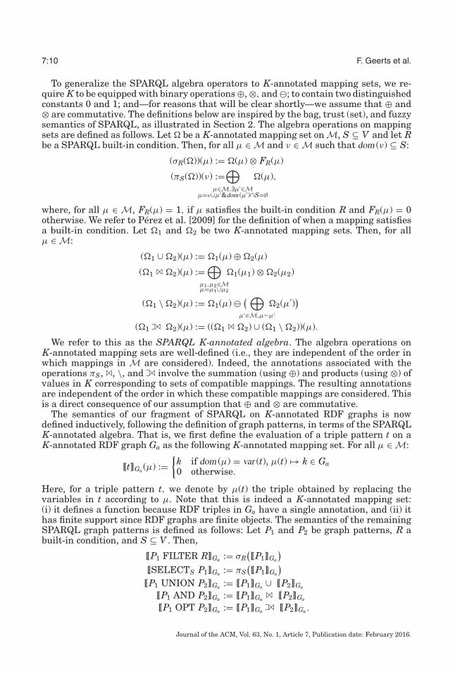
Table I. Translation from SPARQL AlgebraTerms to Annotation Terms
by Means of the Mapping s-to-a
SPARQL s-to-a AnnotationPi → xi∅ → 0e1 ∪ e2 → s-to-a(e1) ⊕ s-to-a(e2)e1 � e2 → s-to-a(e1) ⊗ s-to-a(e2)e1 \ e2 → s-to-a(e1) � s-to-a(e2)σ?x=?x(e1) → s-to-a(e1) ⊗ 1In this table, Pi is a variable represent-ing a graph pattern, and e1 and e2 areSPARQL algebra terms. Similarly, xi isa variable representing values in K.
in K, and closed under ⊕, ⊗, �. Table I shows the inductive definition of the mappings-to-a from SPARQL terms to annotation terms.
LEMMA 4.1. If e1 ≡ e2 is a restricted SPARQL K-annotated algebra equivalence, thens-to-a(e1) = s-to-a(e2) is an identity that holds on (K,⊕,⊗,�, 0, 1).
PROOF. Let e1 ≡ e2 be a SPARQL K-annotated algebra equivalence. For simplic-ity and without loss of generality, assume that e1 and e2 are SPARQL terms overthe variables P1, . . . , Pn. Consider the K-annotated RDF graph Ga consisting of ntriples (ai, b, c) �→ ki such that a1, . . . , an are n distinct constants, b and c are ar-bitrary constants, and k1, . . . , kn are arbitrary values taken from K. Furthermore,let Qi := π?y,?z(σ?x=ai (?x, ?y, ?z)) for i ∈ [1, n]. We denote by e1[[[Q1]]Ga
, . . . , [[Qn]]Ga]
the SPARQL graph pattern obtained by substituting each occurrence of the vari-able Pi with the K-annotated mapping set [[Qi]]Ga
, for i ∈ [1, n], and, similarly, fore2[[[Q1]]Ga
, . . . , [[Qn]]Ga]. Along the same lines, for an annotation term t over variables
x1, . . . , xn, we denote by t[k1, . . . , kn] the element in K obtained by substituting occur-rences of xi by the value ki, for i ∈ [1, n].
Observe the following. It is readily verified that [[Qi]]Ga= {(b, c) �→ ki} for i ∈ [1, n].
Furthermore, for i, j ∈ [1, n], we have that (i) [[Qi ∪ Qj]]Ga= {(b, c) �→ ki ⊕ kj};
(ii) [[Qi � Qj]]Ga= {(b, c) �→ ki ⊗ kj}; (iii) [[Qi \ Qj]]Ga
= {(b, c) �→ ki � kj}; and(iv) [[σ?w=?w(Qi)]]Ga
= {(b, c) �→ ki ⊗ 1}, for w ∈ {y, z}. From this, and by inductionon the structure of the terms e1 and e2, we can conclude that
ei[[[Q1]]Ga, . . . , [[Qn]]Ga
] = {(b, c) �→ s-to-a(ei)[k1, . . . , kn]},for i = 1, 2. Hence, e1 ≡ e2 implies that s-to-a(e1)[k1, . . . , kn] = s-to-a(e2)[k1, . . . , kn] andthis for arbitrary choices of k1, . . . , kn. In other words, s-to-a(e1) = s-to-a(e2) is an identityon K.
The choice of annotation structure thus entirely depends on the SPARQL equiva-lences that one would like to be satisfied when evaluating SPARQL on K-annotatedRDF graphs.
We next propose a set of equivalences that are desired to hold when evaluatingSPARQL on K-annotated RDF graphs.
4.2. SPARQL Equivalences for the Positive Fragment
Consider first the positive fragment of the SPARQL algebra (i.e., the fragment thatdoes not include \ and �). It has been noted [Schmidt et al. 2010] that the followingSPARQL algebra equivalences hold in the case of set and bag semantics and thus arenatural to impose in the general K-annotated setting: For any K-annotated mapping
Journal of the ACM, Vol. 63, No. 1, Article 7, Publication date: February 2016.

Algebraic Structures for Capturing the Provenance of SPARQL Queries 7:13
Fig. 2. Axiomatization A of spm-semirings.
sets �1, �2, and �3, we have that
E1 ={
σ?x=?x(�1) ≡ �1 �1 � ∅ ≡ ∅ �1 ∪ ∅ ≡ �1 �1 ∪ �2 ≡ �2 ∪ �1�1 � �2 ≡ �2 � �1 �1 ∪ (�2 ∪ �3) ≡ (�1 ∪ �2) ∪ �3�1 � (�2 � �3) ≡ (�1 � �2) � �3 �1 � (�2 ∪ �3) ≡ (�1 � �2) ∪ (�1 � �3)
}.
The following proposition is a direct consequence of Lemma 4.1. Indeed, the SPARQLequivalences in E1 precisely correspond to the set of identities shown as id1–id8 inFigure 2. These identities define algebraic structures better known as semirings.
PROPOSITION 4.2. If the positive fragment of the SPARQL K-annotated algebra isrequired to satisfy the equivalences in E1, then (K,⊕,⊗, 0, 1) must be a semiring. Fur-thermore, if (K,⊕,⊗, 0, 1) is a semiring, then the positive SPARQL algebra operatorspreserve the finiteness of support. In particular, for any positive SPARQL graph patternP and K-annotated RDF graph Ga, [[P]]Ga has a finite support.
PROOF. Lemma 4.1 implies that the equivalences in E1 correspond to the semiringidentities id1–id8 shown in Figure 2. We next show that the positive algebra operatorspreserve the finiteness of support. That is, if �, �1, and �2 are K-annotated mappingsets, then σR(�), πS(�), �1 ∪ �2, and �1 � �2 are K-annotated mapping sets as well(i.e., they have finite support). For σR(�), it is readily verified that σR(�) is containedin the support of �. Indeed, this follows from the fact that k ⊗ 1 = k and k ⊗ 0 = 0hold in semirings. Let μ and ν be mappings in M such that dom (ν) ⊆ S ⊆ V . Then,(πS(�))(ν) �= 0 iff there exists a μ′ ∈ M such that μ = ν ∪ μ′, dom (μ′) ∩ S = ∅ and,furthermore, �(μ) �= 0. Indeed, suppose that for all such mapping μ ∈ M, �(μ) = 0,then (πS(�))(ν) = 0 ⊕ · · · ⊕ 0 = 0 since 0 ⊕ 0 = 0 holds in semirings. Hence, since �has finite support so does πS(�). Similarly, (�1 ∪ �2)(μ) �= 0 if and only if �1(μ) �= 0or �2(μ) �= 0. Finally, (�1 � �2)(μ) �= 0 if and only if there exist μ1, μ2 ∈ M suchthat μ = μ1 ∪ μ2 and �1(μ1) �= 0 and �2(μ2) �= 0. Indeed, this follows again from thefact that k ⊗ 0 = 0 holds in semirings. Hence, since �1 and �2 have finite supportso do �1 ∪ �2 and �1 � �2. To show that [[P]]Ga has finite support for any positiveSPARQL graph pattern P and K-annotated RDF graph Ga, it suffices to observe that(i) the support of [[t]]Ga for a triple pattern t is finite since Ga consists of finitely manytriples, and (ii) [[P]]Ga is defined inductively in terms of the positive algebra operatorsand triple patterns. Given that these operators preserve the finiteness of support, wemay conclude that [[P]]Ga has finite support, as desired.
Journal of the ACM, Vol. 63, No. 1, Article 7, Publication date: February 2016.

7:14 F. Geerts et al.
4.3. SPARQL Equivalences Involving Difference
We next turn our attention to the full SPARQL fragment including the optional oper-ator. More specifically, in view of the relationship between � and \, we focus on the \operator.
The examples given in Section 2 suggest that the � operator corresponding to \ is tosatisfy
k1 � k2 ={
k1 if k2 = 0; and0 otherwise.
(†)
Unfortunately, if we want to stay within the setting of algebraic structures defined byidentities (i.e., equational varieties), then � cannot be defined as in (†).
PROPOSITION 4.3. The class of algebraic structures of the form (K,⊕,⊗,�, 0, 1) thatsatisfy that for any k1, k2 ∈ K, k1 � k2 = k1 in case k2 = 0, and k1 � k2 = 0 otherwise, isnot an equational variety.
PROOF. This is an immediate consequence of Birkhoff ’s Theorem (see, e.g., The-orem 11.9 in Burris and Sankappanavar [1981]), which says that classes of alge-braic structures defined by identities (i.e., equational varieties) are precisely thosewhich are closed under taking homomorphisms, subalgebras, and products. Suppose,for the sake of contradiction, that identities exist that define the desired �, and denoteby V the corresponding variety. Let (K,⊕K,⊗K,�K, 0K, 1K) and (L,⊕L,⊗L,�L, 0L, 1L)be two algebraic structures in V. Consider the canonical �K,L operator on the prod-uct K × L defined as (k1, 1) �K,L (k2, 2) = (k1 �K k2, 1 �L 2). The operations⊕K,L, ⊗K,L, and constants 0K,L and 1K,L are defined similarly. Then, by assump-tion, V is a variety, and Birkhoff ’s Theorem implies that V must be closed undertaking products. Hence, (K × L,⊕K,L,⊗K,L,�K,L, 0K,L, 1K,L) must be a structure inV and thus (1K, 1L) �K,L (0K, 1L) should be equal to 0K,L. However, observe that(1K, 1L) �K,L (0K, 1L) = (1K, 0L) �= (0K, 0L) = 0K,L, by the definition of �K,L. This showsthat V is not closed under taking products, a contradiction. Hence, no set of identitiesexists that defines the desired �.
In view of Proposition 4.3, we cannot use SPARQL equivalences to precisely capturethe intended semantics of � as given by (†). Not all is lost, however. In the following, wedefine an equational variety of so-called spm-semirings (K,⊕,⊗,�, 0, 1) that (i) extendsthe class of semirings and (ii) encompasses spm-semirings in which � satisfies (†). Notethat Proposition 4.3 implies that there must be spm-semirings for which � does notsatisfy (†). However, we will see later that (†) holds in most practical cases.
To define spm-semirings, we leverage Lemma 4.1. That is, we gain inspiration fromknown SPARQL algebra equivalences that involve \ and then translate those into iden-tities involving �. More specifically, we consider the following SPARQL equivalencesthat involve \ and that hold under the set and bag semantics [Schmidt et al. 2010]. Forany K-annotated mapping sets �1, �2, and �3:
E2 ={
�1 \ �1 ≡ ∅ �1 \ (�2 ∪ �3) ≡ (�1 \ �2) \ �3�1 � (�2 \ �3) ≡ (�1 � �2) \ �3 (cond)
}.
The last equivalence is not given in Schmidt et al. [2010] and does not hold in general.It does hold, however, under mild conditions (denoted by cond) on the mapping setsinvolved. For instance, the equivalence holds when cond requires that any mapping in�3 that is compatible with a mapping in �2 is also compatible with a mapping in �1. Itis easy to see that Lemma 4.1 still applies to such equivalences since the proof of thatlemma uses mapping sets that satisfy this condition.
Journal of the ACM, Vol. 63, No. 1, Article 7, Publication date: February 2016.

Algebraic Structures for Capturing the Provenance of SPARQL Queries 7:15
We further identify the following equivalence: For any K-annotated mapping set �1and �2, we have that
E3 = {(�1 \ (�1 \ �2)) ∪ (�1 \ �2) ≡ �1}.This equivalence also holds in all settings we have considered so far. By imposingE1, E2, and E3 on the SPARQL K-annotated algebra, we obtain a generalization ofProposition 4.2 that accommodates for the difference (\) and optional operator ( �).The proof again relies on Lemma 4.1.
PROPOSITION 4.4. If the SPARQL K-annotated algebra is required to satisfy the equiv-alences in E1, E2, and E3, then (K,⊕,⊗,�, 0, 1) is an algebraic structure satisfying theidentities shown in Figure 2. Furthermore, in this case, the SPARQL algebra operatorspreserve the finiteness of support. In particular, for any SPARQL graph pattern P andK-annotated RDF graph Ga, [[P]]Ga has a finite support.
PROOF. This is verified in precisely the same way as in the proof of Proposition 4.2by using E1, E2, and E3 instead of E1 and by using id1–id12 as shown in Figure 2 ratherthan only id1–id8. To show that the algebra operators preserve the finiteness of support,it suffices to show that if �1 and �2 are K-annotated mapping sets, then so is �1\�2.Indeed, we already established that the positive operators preserve the finiteness ofsupport in Proposition 4.2, and �1 � �2 is defined in terms of ∪, �, and \. Let μ bea mapping in M. Observe that (�1 \ �2)(μ) can be different from 0 only if �1(μ) �= 0.Indeed, this follows from the fact that 0 � k = 0 holds in spm-semirings:
0 � k = (0 ⊗ 1) � k (by id1)
= 0 ⊗ (1 � k) (by id11)
= 0. (by id2)
Finally, in precisely the same way as in Proposition 4.2, one can verify that [[P]]Ga hasa finite support for any SPARQL expression P and K-annotated RDF graph Ga.
Definition 4.5. An spm-semiring is an algebraic structure (K,⊕,⊗,�, 0, 1) thatsatisfies the identities id1–id12 given in Figure 2. Here, “spm” stands for “SPARQLminus.” The class of spm-semirings thus forms an equational variety.
Proposition 4.4 thus implies that spm-semirings are a good candidate annota-tion structure when considering SPARQL on annotated RDF. It can be readilyverified that (N,+,×,−bag, 0, 1), ({true, false},∨,∧,−trust, false, true), and ([0, 1], max,min,−fuzzy, 0, 1) are spm-semirings. We will see more examples of spm-semirings inthe next section.
4.4. Minimality
We next address the minimality of the set of identities that define spm-semirings. LetI be a set of identities and K an algebraic structure. We say that K satisfies I, denotedby K |= I, if K satisfies all identities in I. Let e be an identity. Then e is implied byI, denoted by I |= e, if for all structures K such that K |= I we have K |= e. Two setsof identities I1 and I2 are said to be equivalent if all identities in I2 are implied by I1and vice versa. A set I of identities is said to be minimal if for all e ∈ I, (I \ e) �|= e. LetA be the set of spm-semiring identities shown in Figure 2.
PROPOSITION 4.6. The sets of identities A and A \ {id2, id3} are equivalent and, further-more, A \ {id2, id3} is minimal. In other words, A \ {id2, id3} is a minimal set of identitiesdefining the class of spm-semirings.
Journal of the ACM, Vol. 63, No. 1, Article 7, Publication date: February 2016.

7:16 F. Geerts et al.
PROOF. Let A′ = A \ {id2, id3}. We first show minimality. It suffices to verify that foreach identity id in A′ there exists a structure that satisfies all identities in A′ \ {id} butviolates id. The list of these structures is deferred to the appendix. For the equivalenceof A and A′, it suffices to verify A′ |= {id2, id3} since A′ ⊂ A. We first show that A′implies that for any k1 ∈ K, 0 ⊕ (k1 � 0) = k1.
k1 = (k1 � (k1 � k2)
)⊕ (k1 � k2) (by id12)
= (k1 � (k1 � k1)
)⊕ (k1 � k1) (for k2 = k1)
= (k1 � 0) ⊕ 0 (by id9)= 0 ⊕ (k1 � 0). (by id4)
In particular, 0 = 0 ⊕ (0 � 0), which in turn is equal to 0 ⊕ 0 by id9. From this, it followsthat A′ |= id3:
k1 = 0 ⊕ (k1 � 0) (by the above identity)= (0 ⊕ 0) ⊕ (k1 � 0) (by 0 = 0 ⊕ 0)= 0 ⊕ (0 ⊕ (k1 � 0)) (by id6)= 0 ⊕ k1 (by the above identity)= k1 ⊕ 0. (by id4)
We can thus safely use id3 to show that A′ |= id2:
k1 ⊗ 0 = k1 ⊗ (k1 � k1) (by id9)= k1 ⊗ (k1 � (k1 ⊗ 1)) (by id1)= k1 ⊗ (k1 � (k1 ⊗ (1 ⊕ 0))) (by id2)= k1 ⊗ (k1 � ((k1 ⊗ 1) ⊕ (k1 ⊗ 0))) (by id8)= k1 ⊗ (k1 � (k1 ⊕ (k1 ⊗ 0))) (by id1)= k1 ⊗ ((k1 � k1) � (k1 ⊗ 0)) (by id10)= k1 ⊗ (0 � (k1 ⊗ 0)) (by id9)= (k1 ⊗ 0) � (k1 ⊗ 0) (by id11)= 0. (by id9)
In other words, A′ |= {id2, id3}.5. CHARACTERIZATION OF SPM-SEMIRINGS
With the definition of spm-semirings at hand, an obvious question is how to constructspm-semirings from algebraic objects that we already know. In this section, we char-acterize the class of spm-semirings in terms of a combination of semirings and booleanalgebras, two standard algebraic structures (Theorem 5.3). Not only does this charac-terization allow us to show that certain structures are spm-semirings, it also opens theway for identifying a universal object in the class of spm-semirings, as will be shownin the next section.
5.1. Seba-Structures: Semirings with an Embedded Boolean Algebra
Recall from Section 4 that we would have preferred � to satisfy (†); that is, for anyk1, k2 ∈ K, k1 � k2 = 0 if k2 �= 0, and k1 � k2 = k1 otherwise. Or, in other words, the valueof k1 � k2 is determined by k1 and whether or not k2 is equal to 0.
To get some inspiration on how to obtain an operator � that satisfies (†) by combiningsemirings with boolean algebras, we consider a semiring K and the two-element boolean
Journal of the ACM, Vol. 63, No. 1, Article 7, Publication date: February 2016.

Algebraic Structures for Capturing the Provenance of SPARQL Queries 7:17
algebra B2 = ({⊥,�},∨,∧, ¯,⊥,�). Observe the following: Assume that we have someway of mapping elements k in K to elements in B2 such that k is mapped to � if k isdifferent from 0 and to ⊥ if k is equal to 0. Let us denote such mapping from K to B2 byd. Furthermore, assume that we can embed the boolean values � and ⊥ to 1 and 0 in K,respectively. Denote such an embedding from B2 to K by ı. Define k1 �k2 := k1 ⊗ ı(d(k2)),where d(k2) is the complement of d(k2). Then clearly, k1 � k2 satisfies (†).
We next identify some properties that these mappings d and ı should have. Clearly,d(1) = � and d(0) = ⊥ must hold for d. Similarly, the mapping ı must satisfy ı(⊥) = 0and ı(�) = 1. These conditions pose some additional restrictions on how the operationsin K interact with the operations in B2. Indeed, one would be tempted to requirethat for elements k1, k2 ∈ K and b1, b2 ∈ B2 we have that d(k1 ⊕ k2) = d(k1) ∨ d(k2),d(k1 ⊗ k2) = d(k1) ∧ d(k2), ı(b1 ∨ b2) = ı(b1) ⊕ ı(b2), and ı(b1 ∧ b2) = ı(b1) ⊗ ı(b2); that is,d and ı are proper embeddings of K in B2 and vice versa, respectively. Some of theserequirements, however, are too restrictive and limit the kind of semirings that we canconsider.
For example, ı(b1 ∨ b2) = ı(b1) ⊕ ı(b2) implies that 1 = ı(�) = ı(� ∨ �) = ı(�) ⊕ ı(�) =1 ⊕ 1, which is a property that does not hold for general semirings K. Instead, we wantthat ı(� ∨ �) = ı(�), ı(� ∨ ⊥) = ı(�) and ı(⊥ ∨ ⊥) = ı(⊥). This can be achieved, forinstance, by defining ı(b1 ∨ b2) = ı(b1) ⊕ (ı(b1) ⊗ ı(b2)) for elements b1, b2 ∈ B2. Indeed,observe that ı(� ∨ �) = ı(�) ⊕ (ı(⊥) ⊗ ı(�)) = ı(�), as desired.
As another example, consider a semiring K with zero divisors; that is, there existk1, k2 ∈ K such that k1 �= 0, k2 �= 0 but k1 ⊗ k2 = 0. Then, ⊥ = d(k1 ⊗ k2) = d(k1) ∧ d(k2) =� ∧ � = � does not hold. Nevertheless, we know that ⊥ = d(k ⊗ 0) = d(k) ∧ ⊥ and,similarly, d(k) = d(k ⊗ 1) = d(k) ∧ � for any k ∈ K. We therefore only require thatd(k ⊗ ı(b)) = d(k) ∧ b for k ∈ K and b ∈ B2.
As we show later, d(k1 ⊕ k2) = d(k1) ∨ d(k2), d(k ⊗ ı(b)) = d(k) ∧ b, ı(b1 ∨ b2) = ı(b1) ⊕(ı(b1) ⊗ ı(b2)), and ı(b1 ∧ b2) = ı(b1) ⊗ ı(b2) allow us to define k1 � k2 := k1 ⊗ ı(d(k2)) ingeneral, provided that we add one more condition involving complementation in B2. Inparticular, since we want that k � k = 0, we assume that k ⊗ ı(d(k)) = 0 holds for dand ı.
In the following definitions, we generalize these observations by means of a so-calledseba-structure that consists of a semiring K together with an embedded boolean algebraB, linked together with mappings d : K → B and ı : B → K.
Definition 5.1. A seba-structure is of the form (K, B, d, ı) where K is a commutativesemiring (K,⊕,⊗, 0, 1), B a boolean algebra (B,∨,∧, ,⊥,�), and d : K → B andı : B → K are mappings such that
sb1: d(0) = ⊥ and d(1) = � sb2: ı(⊥) = 0 and ı(�) = 1sb3: d(k1 ⊕ k2) = d(k1) ∨ d(k2) sb4: ı(b1 ∨ b2) = ı(b1) ⊕ (
ı(b1) ⊗ ı(b2))
sb5 : d(k ⊗ ı(b)) = d(k) ∧ b sb6: ı(b1 ∧ b2) = ı(b1) ⊗ ı(b2)sb7: k ⊗ ı(d(k)) = 0.
Given this, we next show how � can be defined in terms of a seba-structure followingour earlier observation.
Definition 5.2. We say that an algebraic structure (L,⊕,⊗,�, 0, 1) is derived froma seba-structure (K, B, d, ı) if (L,⊕,⊗, 0, 1) and (K,⊕,⊗, 0, 1) coincide and for anyk, ∈ L, k � = k ⊗ ı(d()).
The main result of this section is that spm-semirings and seba-structures are closelyrelated.
Journal of the ACM, Vol. 63, No. 1, Article 7, Publication date: February 2016.
7:18 F. Geerts et al.
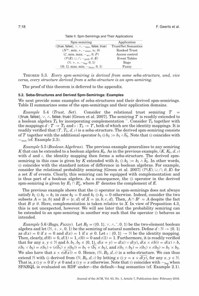
Table II. Spm-Semirings and Their Applications
Spm-semiring Application({true, false}, ∨,∧, −trust, false, true) Trust/Set Semantics
(N∞, min, +,−rtrust, ∞, 0) Ranked Trust(C, min, max, −acc, 0, P) Access control(P(E), ∪,∩, −prob, ∅, E) Event Tables
(N,+, ×, −bag, 0, 1) Bags([0, 1], max, min, −fuzzy, 0, 1) Fuzzy
THEOREM 5.3. Every spm-semiring is derived from some seba-structure, and, viceversa, every structure derived from a seba-structure is an spm-semiring.
The proof of this theorem is deferred to the appendix.
5.2. Seba-Structures and Derived Spm-Semirings: Examples
We next provide some examples of seba-structures and their derived spm-semirings.Table II summarizes some of the spm-semirings and their application domains.
Example 5.4 (Trust, Set). Consider the relational trust semiring T =({true, false},∨,∧, false, true) [Green et al. 2007]. The semiring T is readily extended toa boolean algebra Tb by incorporating complementation . Consider Tb together withthe mappings d : T → Tb and ı : Tb → T , both of which are the identity mappings. It isreadily verified that (T , Tb, d, ı) is a seba-structure. The derived spm-semiring consistsof T together with the additional operator b1 �b2 := b1 ∧b2. Note that � coincides with−trust (cf. Example 2.3).
Example 5.5 (Boolean Algebras). The previous example generalizes to any semiringK that can be extended to a boolean algebra Kb. As in the previous example, (K, Kb, d, ı)with d and ı, the identity mapping then forms a seba-structure. The derived spm-semiring in this case is given by K extended with k1 � k2 := k1 ∧ k2. In other words,� coincides with the standard notion of difference in boolean algebras. For example,consider the relational probability semiring [Green et al. 2007] (P(E),∪,∩,∅, E) fora set E of events. Clearly, this semiring can be equipped with complementation andis thus part of a boolean algebra. As a consequence, the � operator in the derivedspm-semiring is given by E1 ∩ Ec
2, where Ec denotes the complement of E.
The previous example shows that the � operator in spm-semirings does not alwayssatisfy k1 � k2 = k1 in case k2 = 0 and k1 � k2 = 0 otherwise. Indeed, consider the twosubsets A = {a, b} and B = {c, d} of X = {a, b, c, d}. Then, A∩ Bc = A despite the factthat B �= ∅. Here, complementation is taken relative to X. In view of Proposition 4.3,this is not unexpected, however. We will see later that the probability semiring canbe extended to an spm-semiring in another way such that the operator � behaves asintended.
Example 5.6 (Bags, Fuzzy). Let B2 = ({0, 1},∨,∧, ¯, 0, 1) be the two-element booleanalgebra and let (N,+,×, 0, 1) be the semiring of natural numbers. Define d : N → {0, 1}as d(x) = 0 if x = 0 and d(x) = 1 if x �= 0. Let ı : {0, 1} → N be the identity mapping.Then, clearly, d(0) = 0, d(1) = 1, ı(0) = 0 and ı(1) = 1. Furthermore, it is readily verifiedthat for any x, y ∈ N and b, b1, b2 ∈ {0, 1}, d(x + y) = d(x) ∨ d(y), d(x × ı(b)) = d(x) ∧ b,ı(b1 ∨ b2) = ı(b1) + (ı(b1) × ı(b2)) = b1 + (b1 × b2), and ı(b1 ∧ b2) = ı(b1) × ı(b2) = b1 × b2.We also have that x × ı(d(x)) = 0. Hence, (N, B2, d, ı) is a seba-structure. We can thusextend N with � derived from (N, B2, d, ı) by letting x � y = x × d(y), for any x, y ∈ N.That is, x� y = 0 if y �= 0 and x� y = x otherwise. Note that � coincides with −bag whenSPARQL is evaluated on RDF under—the default—bag semantics (cf. Example 2.1).
Journal of the ACM, Vol. 63, No. 1, Article 7, Publication date: February 2016.

Algebraic Structures for Capturing the Provenance of SPARQL Queries 7:19
Along the same lines, the fuzzy semiring F = ([0, 1], max, min, 0, 1) can be extendedwith � derived from (F, B2, d, ı) with d and ı, as above. Note that, in this case, p � q =min{p, d(q)} is equal to 0 if q �= 0, and is p otherwise; that is, � coincides with −fuzzy,as desired (cf. Example 2.4).
Example 5.7 (Zero-Sum Free Semirings). The previous example can be generalizedto arbitrary zero-sum free semirings. Recall that a semiring K is zero-sum free if forany k, ∈ K we have that k ⊕ = 0 implies that both k and are 0. It is readilyverified that for such K, (K, B2, d, ı) is a seba-structure, where d(k) = 0 if k = 0 andd(k) = 1 if k �= 0, and ı(0) = 0K and ı(1) = 1K. The � operator in the derived structureis consequently defined as k � := k ⊗ ı(d()).
The restriction to zero-sum free semirings in the previous example is necessary.Indeed, let (K, B, d, ı) be a seba-structure and assume that k ⊕ = 0. Then alsod(k ⊕ ) = ⊥ = d(k)∨d() and hence both d(k) = ⊥ and d() = ⊥. We claim that d(k) = ⊥if and only if k = 0. Suppose, for the sake of contradiction, that d(k) = ⊥ for k �= 0.Then, from 0 �= k = k ⊗ ı(d(k)) = 0 we obtain a contradiction. Similarly, for d() = ⊥.
Example 5.8 (Probability). Let us reconsider the probability semiring (P(E),∪,∩,∅, E). Clearly, this semiring is zero-sum free, and the previous example tells us thata seba-structure can be obtained as follows: For any event Ei ⊆ E, d(Ei) = 1 if Ei �= ∅and d(Ei) = 0 otherwise, and ı(0) = ∅ and ı(1) = E. In other words, we map events inP(E) to the two-element boolean algebra B2 such that the empty event is mapped to 0and all non-empty events are mapped to 1. As a consequence, the operator Ei � Ej onP(E) in the derived spm-semiring is defined by Ei ∩ ı(d(Ej)) and results in Ei when Ej isempty and in ∅ otherwise. To relate the semantics of Ei � Ej with the standard possibleworld semantics of probabilistic RDF and the certain answer interpretation of SPARQL(see, e.g., Kementsietsidis et al. [2014]) observe the following. If the probability p(Ej)of Ej is zero, then there is no possible world in which Ej appears, and thus Ei shouldbe returned in every possible world. The certain answers thus would be Ei, consistentwith Ei � Ej . In contrast, if p(Ej) > 0, then there is at least one world in which Ej isreturned, and, on this world, an empty result should be returned. As a consequence,the certain answer would be empty as well, consistent with Ei � Ej . We also denote �by −prob.
Example 5.9 (Ranked Trust, Access Policy). Consider the tropical semiring (N∞, min,+,∞, 0) [Green et al. 2007], where N
∞ is short for N ∪ {∞}. This semiring has beenused to model ranked trust for relational queries [Karvounarakis et al. 2010] and canbe regarded as a generalization of the boolean trust semiring. In the case of RDFdata, triples that are completely untrusted and should be disregarded have ∞ astheir rank, whereas completely trusted triples have rank 0. Clearly, this is a zero-sum-free semiring, and, similarly to the previous examples, one can extend it to anspm-semiring such that m −rtrust n = ∞ in case n �= ∞, and m −rtrust n = m otherwise.Along the same lines, one can extend the semiring (C, min, max, 0, P) [Foster et al.2008], with C = {P(ublic), C(onfidential), S(ecret), T (op Secret), 0}, used in the contextof confidentiality policies, to an spm-semiring. Here, the order between the levels ofaccess is specified as P < C < S < T < 0, and the operators min and max aredefined relative to this order. It is readily verified that, in the resulting spm-semiring,v −accw = v if w is 0 and can thus be ignored, and v −accw = 0 otherwise.
6. UNIVERSAL SPM-SEMIRING
The importance of the universal “most general” object in a class of algebraic structureshas already been emphasized in the relational context [Green et al. 2007]. Indeed, in
Journal of the ACM, Vol. 63, No. 1, Article 7, Publication date: February 2016.

7:20 F. Geerts et al.
that setting, semirings are the appropriate annotation structure and the semiring ofpolynomials (N[X],+, ·, 0, 1) is known to be universal. It has been shown that the evalu-ation of positive relational algebra expressions on semiring-annotated relations factorsthrough the evaluation on relations that take their annotations from (N[X],+, ·, 0, 1)[Green et al. 2007]. This implies, among other things, that it suffices to extend positiverelational algebra evaluation algorithms to relations that are annotated with valuesin the universal object from which the query results on specific annotation structures(semirings) can then easily be obtained. In this section, we first identify a universalobject in the class of seba-structures for which we then show that the derived structureis a universal spm-semiring. In Section 7, we establish a factorization property forSPARQL evaluation by leveraging this universal spm-semiring.
6.1. Universal Seba-Structure
We first define the notion of universal seba-structure. Let (K1,⊕1,⊗1, 01, 11) and(K2,⊕2,⊗2, 02, 12) be two semirings; (B1,∨1,∧1,
1,⊥1,�1) and (B2,∨2,∧2,2,⊥2,�2)
be two boolean algebras; and d1 : K1 → B1, d2 : K2 → B2, ı1 : B1 → K1 and ı2 : B2 → K2be mappings such that (K1, B1, d1, ı1) and (K2, B2, d2, ı2) are seba-structures. We saythat a mapping (h, β) : (K1, B1) → (K2, B2) is a seba-homomorphism if the followingconditions are satisfied:
—The mapping h is a semiring homomorphism from K1 to K2. That is, for any k, k′ ∈ K1,h(k ⊕1 k′) = h(k) ⊕2 h(k′), and h(k ⊗1 k′) = h(k) ⊗2 h(k′). Furthermore, h(01) = 02 andh(11) = 12.
—The mapping β is a boolean algebra homomorphism from B1 to B2. That is, for any
b, b′ ∈ B1, β(b∨1 b′) = β(b)∨2 β(b′), β(b∧1 b′) = β(b)∧2 β(b′), β(b)2 = β(b
1), β(⊥1) = ⊥2,
β(�1) = �2; and finally,—β(d1(k)) = d2(h(k)) and h(ı1(b)) = ı2(β(b)).
Let X = {x1, . . . , xn} be a finite set of variables. A semiring (K,⊕,⊗, 0, 1) is said to befinitely generated by X if it is the smallest semiring such that X ⊆ K. A seba-structure(K, B, d, ı) is finitely generated by X if its semiring is finitely generated by X. We saythat (K, B, d, ı) is freely generated by X if it is generated by X, and, in addition, forevery seba-structure (K1, B1, d1, ı1) and any valuation ν : X → K1, we can uniquelyextend ν to a seba-homomorphism (h, β) from (K, B, d, ı) to (K1, B1, d1, ı1) such that hcoincides with ν on X. In this case, we call (K, B, d, ı) a universal object in the class ofseba-structures relative to the generator set X. It can be shown that such a universalobject is unique up to isomorphism (using seba-isomorphisms). We refer to Burris andSankappanavar [1981] for the general theory of universal objects.
A few comments are in order here:(1) It may seem surprising that no explicit set of generators for the boolean algebra Bis provided. The reason is that the generators for B are determined by X as well. To seethis, observe that in a seba-structure (K, B, d, ı), it is always the case that B = d(K).Indeed, for any element b ∈ B, ı(b) ∈ K and d(ı(b)) = d(1 ⊗ ı(b)) = d(1) ∧ b = � ∧ b = b.If K is finitely generated by X, then we have that X ⊆ K and, consequently, K containsall terms built up from elements in X, 0, 1 and using the semiring operations ⊕ and ⊗.Clearly, Bmust contain d(0) and d(1). Furthermore, sb3 tells us that d is compatible with⊕, and thus elements in B are determined by d(μ), where μ belongs to the set mon(X)of monomials over X. For example, if X = {x1, x2} then mon(X) = {x⊗m
1 ⊗ x⊗n2 | m, n � 0}
where x⊗m1 = x1 ⊗ · · · ⊗ x1︸ ︷︷ ︸
m-times
, similarly for x⊗n2 . For ease of notation, we often use the
empty notation instead of ⊗ and simply write xm1 , xn
2 , and xm1 xn
2 instead of x⊗m1 , x⊗n
2 andx⊗m
1 ⊗ x⊗n2 , respectively. For instance, for X = {x1, x2}, we write mon(X) = {1 = x0
1 x02 ,
Journal of the ACM, Vol. 63, No. 1, Article 7, Publication date: February 2016.

Algebraic Structures for Capturing the Provenance of SPARQL Queries 7:21
x1, x2, x21 , x1x2, x2
2 , x31 , . . .}. We thus have that B can be regarded as the smallest boolean
algebra that contains d(0), d(1), and d(μ) for μ ∈ mon(X). The generators of B are thusimplicitly determined by 0, 1, X, and the mapping d : K → B.(2) For a mapping (h, β) : (K1, B1) → (K2, B2) to be a seba-homomorphism, itsuffices that h is a semiring homomorphism, β is compatible with complementa-tion, and β(d1(k)) = d2(h(k)) and h(ı1(b)) = ı2(β(b)) hold. To see this, observe that
β(b ∨1 b′) = β(b1 ∧1 b′1
1
) = β(b1 ∧1 b′1)
2
. Furthermore, β(b1 ∧1 b′1) = β(d1(ı1(b
1) ⊗1
ı1(b′1))) = d2(h(ı1(b1)) ⊗2 h(ı2(b′1))), which in turn is equal to d2(ı2(β(b)
2) ⊗2 ı2(β(b′)
2)) =
β(b)2 ∧2 β(b′)
2. Hence, β(b ∨1 b′) = β(b) ∨2 β(b′). In a similar way, one can verify that
β(b ∧1 b′) = β(b) ∧2 β(b′). Finally, β(�1) = β(d1(11)) = d2(h(11)) = d2(12) = �2 andsimilarly, β(⊥1) = ⊥2.
In the following, we construct a universal seba-structure by extending polynomialswith boolean variables. More specifically, we first define a semiring of so-called booly-nomials. Second, we show that this semiring has a boolean algebra embedded in it.The elements of this algebra correspond to polynomials consisting of boolean variablesonly. Finally, we define the mappings d and ı between the semiring and boolean algebraand show that, all combined, these form a seba-structure.
6.2. Semiring of Boolynomials
Let X = {x1, . . . , xn} be a set of variables and mon(X) be the set of monomials over X.We define two other sets of variables, denoted by BX and BX, that are disjoint from X,as follows: BX = {bμ | μ ∈ mon(X)} and BX = {bμ | μ ∈ mon(X)}. To simplify notation, wedenote the set of variables X ∪ BX ∪ BX by XB.
Let N[XB] be the set of polynomials with coefficients in N over the variables XB. Thesemiring of boolynomials is then defined as follows:
First, we define a congruence relation θ on the semiring of polynomials(N[XB],+, ·, 0, 1) indicating when two polynomials are considered to be equivalent.Recall that θ is a congruence relation on N[XB] if it is an equivalence relation satis-fying the additional conditions that if (p[XB], q[XB]) ∈ θ and (p′[XB], q′[XB]) ∈ θ, then(p[XB] + p′[XB], q[XB] + q′[XB]) ∈ θ and (p[XB] · p′[XB], q[XB] · q′[XB]) ∈ θ .
Second, we consider the quotient semiring of N[XB] with respect to θ . This semiringhas as elements the equivalence classes [p[XB]] consisting of all polynomials that arecongruent to p[XB], operations [p[XB]] + [q[XB]] = [p[XB] + q[XB]], [p[XB]] · [q[XB]] =[p[XB] · q[XB]], and constants [0] and [1].
Definition 6.1. The semiring of boolynomials is the quotient semiring of(N[XB],+, ·, 0, 1) with respect to θ . We denote this semiring by (Nθ [XB],+, ·, 0, 1)3.
It remains to define the congruence relation θ . Intuitively, this relation is to capturethat the variables in BX and BX represent booleans such that bμ indicates that themonomial μ is considered being evaluated to a non-zero element, whereas bμ indicatesthe opposite. We define θ as the smallest congruence relation on N[XB] such that itcontains the following pairs (equivalences). For all monomials μ ∈ mon(X):
(i) (bμ · bμ, 0) ∈ θ and (bμ + bμ, 1) ∈ θ , indicating that bμ and bμ are complements.(ii) (bμ+bμ, bμ) ∈ θ and (bμ+bμ, bμ) ∈ θ , to indicate that “+” is idempotent for variables
in BX and BX.(iii) (bμ ·μ, 0) ∈ θ indicating that the presence of bμ implies that μ should be evaluated
to zero.
3We abuse notation and use +, ·, 0, and 1 for the operations and constants in Nθ [XB], respectively.
Journal of the ACM, Vol. 63, No. 1, Article 7, Publication date: February 2016.
7:22 F. Geerts et al.
(iv) (bμ · bν, bμ) ∈ θ whenever μ = ν · ν ′ for some monomial ν ′, indicating that wheneverμ evaluates to non-zero, then any more general monomial ν evaluates to non-zeroas well. Here, ν is more general than μ if μ = ν · ν ′ for some monomial ν ′.
Note that (i) and (ii) imply that [bμ] = [bμ] · ([bμ] + [bμ]) = [bμ] · [bμ] and [bμ] = [bμ] ·([bμ]+[bμ]) = [bμ]·[bμ]. In other words, also “·” is idempotent for variables in BX and BX.Furthermore, (i) and (iii) imply that [μ] = ([bμ]+[bμ])·[μ] = [bμ]·[μ]+[bμ]·[μ] = [bμ]·[μ].That is, the presence of μ implies the presence of bμ. In addition, from (i) and (iv) itfollows that [bν] = ([bμ] + [bμ]) · [bν] = [bμ] · [bν] + [bμ] · [bν] = [bμ] · [bν] · [bν] + [bμ] · [bν] =[bμ] · [bν] whenever μ = ν · ν ′. That is, whenever ν evaluates to zero then so doesevery more specific monomial μ. Here, μ is more specific than ν if μ = ν · ν ′ for somemonomial ν ′. Also observe that [1] = [b1] and [0] = [b1] where b1 corresponds to theconstant monomial 1 = x0
1 ⊗ · · · ⊗ x0n.
To gain some insight in the semiring of boolynomials, we next provide a procedurefor deciding whether [p[XB]] = [q[XB]] for p[XB] and q[XB] in N[XB]. In a nutshell, witheach polynomial p[XB] in N[XB], we first associate a special representative pe[XB] inits equivalence class [p[XB]], called the expanded version of p[XB]. Then, we show that[p[XB]] = [q[XB]] if and only if pe[XB] is “almost the same” as qe[XB]. We make thismore precise later. The expanded versions are also shown to be useful for identifyingrepresentatives in the sum and product of equivalence classes.
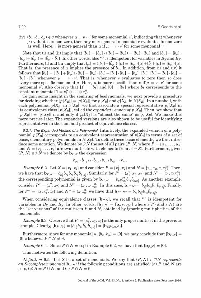
6.2.1. The Expanded Version of a Polynomial. Intuitively, the expanded version of a poly-nomial p[XB] corresponds to an equivalent representation of p[XB] in terms of a set ofbasic, elementary polynomials in N[XB]. To define these basic elements, we first intro-duce some notation. We denote by PN the set of all pairs (P, N) where P = {μ1, . . . , μk}and N = {ν1, . . . , ν} are two multisets with elements from mon(X). Furthermore, given(P, N) ∈ PN we denote by bP,N the expression
bμ1 · bμ2 · · · bμk · bν1 · bν2 · · · bν.
Example 6.2. Let X = {x1, x2} and consider P = {x21 , x2} and N = {x1, x2, x1x3
2}. Then,we have that bP,N = bx2
1bx2 bx1 bx2 bx1x3
2. Similarly, for P ′ = {x2
1 , x2, x2} and N′ = {x1, x1x32},
the corresponding polynomial is given by bP ′,N′ = bx21b2
x2bx1 bx1x3
2. As another example,
consider P ′′ = {x21 , x2} and N′′ = {x1, x1x3
2}. In this case, bP ′′,N′′ = bx21bx2 bx1 bx1x3
2. Finally,
for P ′′′ = {x1, x21 , x2} and N′′′ = {x1x3
2} we have that bP ′′′,N′′′ = bx1bx21bx2 bx1x3
2.
When considering equivalence classes [bP,N], we recall that “·” is idempotent forvariables in BX and BX. In other words, [bP,N] = [bs(P),s(N)] where s(P) and s(N) arethe “set versions” of the multisets P and N, obtained by ignoring multiplicities of themonomials.
Example 6.3. Observe that P ′ = {x21 , x2, x2} is the only proper multiset in the previous
example. Clearly, [bP ′,N′ ] = [bx21bx2 bx1 bx1x3
2] = [bs(P ′),s(N′)].
Furthermore, since for any monomial μ, [bμ · bμ] = [0], we may conclude that [bP,N] =[0] whenever P ∩ N �= ∅.
Example 6.4. Since P ∩ N = {x2} in Example 6.2, we have that [bP,N] = [0].
This motivates the following definition.
Definition 6.5. Let S be a set of monomials. We say that (P, N) ∈ PN representsan S-complete monomial bP,N if the following conditions are satisfied: (a) P and N aresets, (b) S = P ∪ N, and (c) P ∩ N = ∅.
Journal of the ACM, Vol. 63, No. 1, Article 7, Publication date: February 2016.

Algebraic Structures for Capturing the Provenance of SPARQL Queries 7:23
Intuitively, when (P, N) ∈ PN represents an S-complete monomial, then every mono-mial μ ∈ S occurs once in bP,N either as bμ or bμ.
Example 6.6. The pairs (P ′′, N′′) and (P ′′′, N′′′) in Example 6.2 represent the S-complete monomials bP ′′,N′′ = bx2
1bx2 bx1 bx1x3
2and bP ′′′,N′′′ = bx1bx2
1bx2 bx1x3
2, respectively, for
S = {x1, x21 , x2, x1x3
2}.Finally, we denote by C(S) the set of pairs (P, N) that represent non-zero S-complete
monomials (i.e., S-complete monomials for which [bP,N] �= [0]). Note that it followsfrom rules (i) and (iv) that (P, N) ∈ C(S) if and only if (P, N) represents an S-completemonomial, and, moreover, for every μ ∈ P there does not exist a ν ∈ N such thatμ = ν · ν ′ for some monomial ν ′.
Example 6.7. Continuing with the previous example, we have that (P ′′, N′′) �∈ C(S).Indeed, note that x2
1 ∈ P ′′, x1 ∈ N′′ and x21 = x1 ·x1. From this, it follows that [bx2
1bx1 ] = [0]
and thus [bP ′′,N′′ ] = [0]. By contrast, (P ′′′, N′′′) ∈ C(S).
The polynomials bP,N for (P, N) ∈ C(S) will play the role of the basic elements usedto define the expanded versions of polynomials in N[XB].
These elements exhibit the following useful properties, as shown in Lemma 6.8. Thelemma is easily verified from the properties of the equivalence relation θ defined earlier,and its proof is deferred to the appendix.
LEMMA 6.8. For any (P, N) ∈ C(S) and (P ′, N′) whose monomials belong to S, we havethat
[bP,N] · [bP ′,N′ ] ={
[bP,N] if s(P ′) ⊆ P and s(N′) ⊆ N[0] otherwise.
(1)
⎡⎣ ∑
(P,N)∈C(S)
bP,N
⎤⎦ = [1], (2)
where s(P ′) and s(N′) denote the “set versions” of P ′ and N′, respectively. In particular,if (P ′, N′) also belongs to C(S), then [bP,N] · [bP ′,N′ ] = [bP,N] if P = P ′ and N = N′; and[bP,N] · [bP ′,N′] = [0] otherwise.
Given a polynomial p[XB] in N[XB], we next identify the set Sp[XB] of monomials thatare relevant for obtaining the expanded version of p[XB]. More precisely, the expandedversion will be constructed in terms of Sp[XB]-complete monomials.
Definition 6.9. Let p[XB] be a polynomial in N[XB]. If p[XB] = a for some constanta ∈ N, then we define Sp[XB] := {1} where 1 is the constant monomial x0
1 · · · x0n. Otherwise,
if p[XB] is not constant, then we define Sp[XB] as the set of all nonconstant monomialsμ ∈ mon(X) that appear in p[XB], either as μ, bμ, or bμ. We will often abbreviate Sp[XB]and simply write Sp instead.
Example 6.10. For p[XB] = bx1x2 x1 + bx1 bx1 x22 + 4bx1b
4x2
x1x2 + bx1x2 x2, Sp ={x1, x2, x2
2 , x1x2}, for q[XB] = x2 +3, Sq = {x2}, for r[XB] = x2, Sr = {x2} and for t[XB] = 5,St = {1}.
We are now ready to define and construct the expanded version, denoted by pe[XB],of a polynomial p[XB]. We first illustrate this construction by means of an example.The general treatment is part of the proof of Proposition 6.14, where in addition theuniqueness of the resulting polynomial pe[XB] will be established.
Journal of the ACM, Vol. 63, No. 1, Article 7, Publication date: February 2016.

7:24 F. Geerts et al.
Example 6.11. Let X = {x1, x2} and consider p[XB] = bx1x2 x1 +bx1 bx1 x22 +4bx1b
4x2
x1x2 +bx1x2 x2. We saw in the previous example that Sp = {x1, x2, x2
2 , x1x2}. We rewrite p[XB]as an equivalent polynomial in terms of Sp-complete polynomials. Observe that C(Sp)corresponds to the following bP,N ’s:
bx1bx2bx22bx1x2 , bx1bx2 bx2
2bx1x2 , bx1bx2bx2
2bx1x2 , bx1bx2 bx2
2bx1x2 , bx1 bx2 bx2
2bx1x2 ,
bx1bx2bx22bx1x2 , bx1bx2 bx2
2bx1x2 , bx1 bx2 bx2
2bx1x2 .
Step 1. We first multiply p[XB] with∑
(P,N)∈C(Sp) bP,N. Observe that this results in anequivalent polynomial by Property (2) in Lemma 6.8. Using Property (1) in Lemma 6.8,we then eliminate all terms that are equivalent to 0 and further simplify each termsuch that every term consists of a basic element bP,N and a polynomial in N[X]. It iseasily verified that the resulting equivalent polynomial is given by
p1[XB] = bx1bx2bx22bx1x2 · 0 + bx1bx2 bx2
2bx1x2 · 0 + bx1bx2bx2
2bx1x2 (x1 + x2)
+ bx1bx2 bx22bx1x2 (x1 + x2) + bx1 bx2 bx2
2bx1x2 (x1 + x2) + bx1bx2bx2
2bx1x2 (x1 + x2 + 4x1x2)
+ bx1bx2 bx22bx1x2 (x1 + x2 + 4x1x2) + bx1 bx2 bx2
2bx1x2 (x1 + x2),
where we grouped terms according to their preceding basic element bP,N. We in-cluded the first two terms to illustrate that not all elements in C(Sp), when multi-plied with p[XB], result in a non-zero term. For example, for the first term, we haveP = {x1, x2, x2
2 , x1x2} and N = ∅, whereas each of the terms in p[XB] contains an ele-ment of the form bμ for μ ∈ Sp. Hence, by Property (1) in Lemma 6.8, bP,N · p[XB] isequivalent to 0 for P = {x1, x2, x2
2 , x1x2} and N = ∅. Similarly for the second zero termin p1[XB].
Step 2. Although we have already eliminated some zero terms in p1[XB] due toProperty (1) in Lemma 6.8, we can further simplify p1[XB] by removing from eachterm those monomials μ that appear together with bμ. Note that, by construction, eachmonomial μ either appears together with bμ or bμ. The resulting equivalent polynomialis the expanded version pe[XB] of p[XB] and is given by
pe[XB] = bx1bx2bx22bx1x2 (x1 + x2) + bx1bx2 bx2
2bx1x2 (x1 + x2) + bx1 bx2 bx2
2bx1x2 x1
+ bx1bx2bx22bx1x2 x2 + bx1bx2 bx2
2bx1x2 x2 + bx1 bx2 bx2
2bx1x2 · 0,
where we included the last zero term to illustrate that bx1 bx2 bx22bx1x2 (x1 + x2) is elim-
inated from p1[XB]. Also note that some terms have been simplified. For example,bx1bx2 bx2
2bx1x2 (x1 + x2 + 4x1x2) in p1[XB] has become bx1bx2 bx2
2bx1x2 x2. The set of remaining
Sp-complete monomials bP,N that occur in pe[XB] together with a non-zero polynomialin N[X] is referred to as the Sp-support of p[XB].
The support of a polynomial in terms of S-complete monomials, for arbitrary sets Sof monomials, is formally defined as follows.
Definition 6.12. Let p[XB] be a polynomial in N[XB] and let S be a subset of mon(X).The S-support of p[XB] is the set
S-supp(p[XB]) := {(P, N) ∈ C(S) | [bP,N · p[XB]] �= [0]}.Observe that two equivalent polynomials p[XB] and q[XB] have the same S-support.
Indeed, [p[XB]] = [q[XB]] implies that [bP,N·p[XB]] = [bP,N·q[XB]] for any (P, N) ∈ C(S).Hence, [bP,N · p[XB]] = [0] if and only if [bP,N · q[XB]] = [0].
Journal of the ACM, Vol. 63, No. 1, Article 7, Publication date: February 2016.

Algebraic Structures for Capturing the Provenance of SPARQL Queries 7:25
Example 6.13. Continuing with the previous example, the Sp-support of p[XB] isthus given by {(P1, N1), (P2, N2), (P3, N3), (P4, N4), (P5, N5)} with P1 = {x1, x2, x2
2 }, N1 ={x1x2}, P2 = {x1, x2}, N2 = {x2
2 , x1x2}, P3 = {x1}, N3 = {x2, x22 , x1x2}, P4 = {x2, x2
2 },N4 = {x1, x1x2}, P5 = {x2}, and N5 = {x1, x2
2 , x1x2}. Consider pe[XB] in the previousexample and denote the polynomials in N[X] accompanying the bP,N ’s by rP1,N1 [X] =rP2,N2 [X] = x1 + x2, rP3,N3 [X] = x1, and rP4,N4 [X] = rP5,N5 [X] = x2, respectively. Then,pe[XB] is equal to
pe[XB] =∑
(P,N)∈Sp-supp(p[XB])
bP,N · rP,N[X],
where each rP,N[X] ∈ N[X] is non-zero and such that none of its monomials appears inN.
The intuition and examples just described lead to the following proposition whosestatement contains the formal definition of expanded version.
PROPOSITION 6.14. Let p[XB] be a polynomial in N[XB]. Then, [p[XB]] = [pe[XB]],where
pe[XB] =∑
(P,N)∈Sp-supp(p[XB])
bP,N · rP,N[X], (‡)
for some non-zero rP,N[X] ∈ N[X] none of whose monomials appears in N. Furthermore,pe[XB] is uniquely determined by p[XB].
Definition 6.15. The expanded version of p[XB] is the polynomial pe[XB] given in (‡)in the statement of Proposition 6.14.
Observe that the expanded version can be of exponential size in the number ofvariables in Sp. The proof of Proposition 6.14 closely follows the construction given inExample 6.11 and is deferred to the appendix.
6.2.2. Testing Equivalence of Polynomials. The expanded versions are particularly usefulwhen testing for equivalence. One may think that [p[XB]] = [q[XB]] if and only ifthey have identical expanded versions pe[XB] = qe[XB]. This is not the case, however,simply because Sp can be different from Sq, and therefore pe and qe are expressed interms of different complete monomials: Sp-complete monomials for pe and Sq-completemonomials for qe. Nevertheless, one can test equivalence of two polynomials by usingexpanded versions built from (Sp ∪ Sq)-complete monomials. Indeed, in both of theseexpansions, the (Sp∪Sq)-complete monomials must carry identical polynomials in N[X].The following proposition provides a necessary and sufficient condition for testing theequivalence of two polynomials in N[XB].
PROPOSITION 6.16. Let p[XB] and q[XB] be two polynomials in N[XB] and let pe[XB] =∑(P,N)∈Sp-supp(p[XB]) bP,N · rP,N[X] and qe[XB] = ∑
(P,N)∈Sq-supp(q[XB]) bP,N · sP,N[X] be theexpanded versions of p[XB] and q[XB], respectively. Then, [p[XB]] = [q[XB]] if and only iffor every (P, N) in (Sp ∪ Sq)-supp(p[XB]), we have that rP|Sp ,N|Sp
[X] = sP|Sq ,N|Sq[X], where
P|Sp ,N|Sp, P|Sq and N|Sq denote the restriction of P and N to Sp and Sq, respectively.
We defer the proof of the proposition to the appendix. The use of the proposition isillustrated in the following example.
Example 6.17. Let X = {x1, x2} and consider the polynomial p[XB] from the previousexample, and the polynomial q[XB] = bx1x2 (x1 + x2). Note that Sq = {x1, x2, x1x2}. Itis readily verified that qe[XB] = bx1bx2 bx1x2 (x1 + x2) + bx1 bx2 bx1x2 x1 + bx1bx2 bx1x2 x2 and
Journal of the ACM, Vol. 63, No. 1, Article 7, Publication date: February 2016.

7:26 F. Geerts et al.
that the Sq-support of q[XB] is given by {(P ′1, N′
1), (P ′2, N′
2), (P ′3, N′
3)} with P ′1 = {x1, x2},
N′1 = {x1x2}, P ′
2 = {x1}, N′2 = {x2, x1x2}, P ′
3 = {x2} and N′3 = {x1, x1x2}. Let sP ′
1,N′1[X] =
x1+x2, sP ′2,N′
2[X] = x1 and sP ′
3,N′3[X] = x2. Then, qe[XB] = bP ′
1,N′1sP ′
1,N′1[X]+bP ′
2,N′2sP ′
2,N′2[X]+
bP ′3,N′
3sP ′
3,N′3[X]. To check whether p[XB] and q[XB] are equivalent, we verify the condition
stated in the previous proposition. Note that Sp ∪ Sq = Sp in this example. Hence, wehave to further expand the Sq-complete monomials to Sp-complete monomials. It iseasily verified that qe[XB] is equivalent to
bx1bx2bx22bx1x2sP ′
1,N′1[X] + bx1bx2 bx2
2bx1x2sP ′
1,N′1[X] + bx1 bx2 bx2
2bx1x2sP ′
2,N′2[X]
+ bx1bx2bx22bx1x2sP ′
3,N′3[X] + bx1bx2 bx2
2bx1x2sP ′
3,N′3[X].
Recall that pe[XB] is equal to
bx1bx2bx22bx1x2 (x1 + x2) + bx1bx2 bx2
2bx1x2 (x1 + x2) + bx1 bx2 bx2
2bx1x2 x1
+ bx1bx2bx22bx1x2 x2 + bx1bx2 bx2
2bx1x2 x2.
We have thus obtained precisely the same polynomials, which are clearly equivalent.For completeness, we formally verify the conditions stated in Proposition 6.16. Recallthe formulation pe[XB] = ∑
(P,N)∈Sp-supp(p[XB]) bP,N ·rP,N[X] of pe[XB] from Example 6.13.Observe that P1|Sq = P2|Sq = P ′
1, N1|Sq = N2|Sq = N′1, P3|Sq = P ′
2, N3|Sq = N′2, P4|Sq =
P5|Sq = P3,′ and N4|Sq = N5|Sq = N′
3. Then, p[XB] and q[XB] are indeed equivalentsince rP1,N1 [X] = rP2,N2 = sP ′
1,N′1[X] = x1 + x2, rP3,N3 [X] = sP ′
2,N′2[X] = x1, and rP4,N4 [X] =
rP5,N5 [X] = sP ′3,N′
3[X] = x2.
As another example, consider p[XB] = bx1x2 x1 and q[XB] = x2. We have that Sp ={x1, x1x2} and Sq = {x1, x2}. Furthermore, pe[XB] = bx1 bx1x2 x1 and qe[XB] = bx1bx2 x2 +bx1bx2 x2. Let P1 = {x1}, N1 = {x1x2}, P ′
1 = {x1, x2}, N′1 = ∅, P ′
2 = {x2}, N′2 = {x1},
rP1,N1 [X] = x1, sP ′1,N′
1[X] = sP ′
2,N′2[X] = x2. Let S = Sp ∪ S1 = {x1, x2, x1x2}. We have that
pe[XB] is equivalent to
bx1bx2 bx1x2rP1,N1 [X] + bx1 bx2 bx1x2rP1,N1 [X],
and qe[XB] is equivalent to
bx1bx2bx1x2sP ′1,N′
1[X] + bx1bx2 bx1x2sP ′
1,N′1[X] + bx1bx2 bx1x2sP ′
2,N′2[X].
Consider P = {x1, x2, x1x2} and N = ∅. Then, P|Sp = {x1, x1x2}, N|Sp = ∅, P|Sq ={x1, x2} = P ′
1, and N|Sq = ∅ = N′1. Since pe[XB] does not have a term corresponding to
({x1, x1x2},∅) (in other words, r({x1,x1x2},∅) = 0), whereas qe[XB] has a term, rP ′1,N′
1[X] = x2,
corresponding to ({x1, x2},∅), we may conclude that p[XB] and q[XB] are not equivalent.
One may wonder what the complexity is of deciding whether two polynomials areequivalent. The following proposition indicates that it is intractable, in general. Theproof of the proposition is deferred to the appendix.
PROPOSITION 6.18. Given two polynomials p[XB] and q[XB] in N[XB], deciding whether[p[XB]] = [q[XB]] holds is coNP-complete.
6.2.3. Computing with Boolynomials. We conclude this section on boolynomials by show-ing that the expanded versions can also be used to compute representatives of sumsand products of equivalence classes. The proof is omitted because it consists of a simpleverification in which the expanded version of the sum and product of expanded versionsare analyzed. Intuitively, when summing two boolynomials p[XB] and q[XB], one cansimply sum their expanded versions, provided that one considers S-complete monomi-als where S = Sp ∪ Sq. Moreover, the S-complete monomials of interest belong to the
Journal of the ACM, Vol. 63, No. 1, Article 7, Publication date: February 2016.
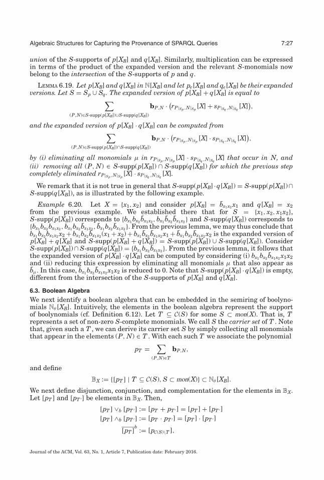
Algebraic Structures for Capturing the Provenance of SPARQL Queries 7:27
union of the S-supports of p[XB] and q[XB]. Similarly, multiplication can be expressedin terms of the product of the expanded version and the relevant S-monomials nowbelong to the intersection of the S-supports of p and q.
LEMMA 6.19. Let p[XB] and q[XB] in N[XB] and let pe[XB] and qe[XB] be their expandedversions. Let S = Sp ∪ Sq. The expanded version of p[XB] + q[XB] is equal to∑
(P,N)∈S-supp(p[XB])∪S-supp(q[XB])
bP,N · (rP|Sp ,N|Sp[X] + sP|Sq ,N|Sq
[X]),
and the expanded version of p[XB] · q[XB] can be computed from∑(P,N)∈S-supp(p[XB])∩S-supp(q[XB])
bP,N · (rP|Sp ,N|Sp[X] · sP|Sq ,N|Sq
[X]),
by (i) eliminating all monomials μ in rP|Sp ,N|Sp[X] · sP|Sq ,N|Sq
[X] that occur in N, and(ii) removing all (P, N) ∈ S-supp(p[XB]) ∩ S-supp(q[XB]) for which the previous stepcompletely eliminated rP|Sp ,N|Sp
[X] · sP|Sq ,N|Sq[X].
We remark that it is not true in general that S-supp(p[XB] ·q[XB]) = S-supp(p[XB])∩S-supp(q[XB]), as is illustrated by the following example.
Example 6.20. Let X = {x1, x2} and consider p[XB] = bx1x2 x1 and q[XB] = x2from the previous example. We established there that for S = {x1, x2, x1x2},S-supp(p[XB]) corresponds to {bx1bx2 bx1x2 , bx1 bx2 bx1x2} and S-supp(q[XB]) corresponds to{bx1bx2bx1x2 , bx1bx2 bx1x2 , bx1bx2 bx1x2}. From the previous lemma, we may thus conclude thatbx1bx2bx1x2 x2 + bx1bx2 bx1x2 (x1 + x2) + bx1 bx2 bx1x2 x1 + bx1bx2 bx1x2 x2 is the expanded version ofp[XB] + q[XB] and S-supp(p[XB] + q[XB]) = S-supp(p[XB]) ∪ S-supp(q[XB]). ConsiderS-supp(p[XB]) ∩ S-supp(q[XB]) = {bx1bx2 bx1x2}. From the previous lemma, it follows thatthe expanded version of p[XB] · q[XB] can be computed by considering (i) bx1bx2 bx1x2 x1x2and (ii) reducing this expression by eliminating all monomials μ that also appear asbμ. In this case, bx1bx2 bx1x2 x1x2 is reduced to 0. Note that S-supp(p[XB] · q[XB]) is empty,different from the intersection of the S-supports of p[XB] and q[XB].
6.3. Boolean Algebra
We next identify a boolean algebra that can be embedded in the semiring of boolyno-mials Nθ [XB]. Intuitively, the elements in the boolean algebra represent the supportof boolynomials (cf. Definition 6.12). Let T ⊆ C(S) for some S ⊂ mon(X). That is, Trepresents a set of non-zero S-complete monomials. We call S the carrier set of T . Notethat, given such a T , we can derive its carrier set S by simply collecting all monomialsthat appear in the elements (P, N) ∈ T . With each such T we associate the polynomial
pT =∑
(P,N)∈T
bP,N,
and define
BX := {[pT ] | T ⊆ C(S), S ⊂ mon(X)} ⊂ Nθ [XB].
We next define disjunction, conjunction, and complementation for the elements in BX.Let [pT ] and [pT ′] be elements in BX. Then,
[pT ] ∨b [pT ′ ] := [pT + pT ′ ] = [pT ] + [pT ′][pT ] ∧b [pT ′ ] := [pT · pT ′] = [pT ] · [pT ′]
[pT ]b
:= [pC(S)\T ],
Journal of the ACM, Vol. 63, No. 1, Article 7, Publication date: February 2016.

7:28 F. Geerts et al.
where S is the carrier set of T . In addition, we define ⊥b and �b as [0] and [1],respectively. It will sometimes be convenient to interpret [0] = [b1] and [1] = [b1],which correspond to the constant polynomials pT = 0 with T = (P = ∅, N = {1}) andpT = 1 with T = (P = {1}, N = ∅), respectively.
In the appendix, we verify that we indeed obtain a boolean algebra:
PROPOSITION 6.21. The operations ∨b, ∧b and b are well-defined and the structure(BX,∨b,∧b,
b,⊥b,�b) is a boolean algebra.
6.4. Universal Seba-Structure
With the semiring of boolynomials (Nθ [XB],+, ·, 0, 1) and boolean algebra (BX,∨b,∧b,
b,⊥b,�b) at hand, we next link them together by means of mappings ıb : BX →Nθ [XB] and db : Nθ [XB] → BX. For ıb, we simply take the identity mapping. That is, for[pT ] ∈ BX we define
ıb([pT ]) := [pT ].
The mapping db is defined as follows. Let p[XB] be a polynomial in N[XB]. We define
db([p[XB]]) := [pSp-supp(p[XB])
],
where Sp is as defined in Definition 6.9. Note that db([0]) = [p{x1}-supp(0)] = [p∅] = [0]and db([n]) = [p{x1}-supp(n)] = [pC({x1})] = [1].
The mapping db is well-defined. Indeed, given [p[XB]] = [q[XB]], we saw thatS-supp(p[XB]) = S-supp(q[XB]) for any S ⊆ mon(X). Moreover, it is easily verifiedthat, for Sp ⊆ S ⊆ S′, [pS-supp(p[XB])] = [pS′-supp(p[XB])]. Hence, db([p[XB]]) is equal to[
pSp-supp(p[XB])] = [
p(Sp ∪ Sq)-supp(p[XB])] = [
p(Sp ∪ Sq)-supp(q[XB])] = [
pSq-supp(q[XB])],
which equals db([q[XB]]).We conclude this section by showing that (Nθ [XB], BX, db, ıb) is indeed a seba-structure
and that it is universal.
THEOREM 6.22. The structure (Nθ [XB], BX, db, ıb) is a seba-structure that is universalin the class of all seba-structures, relative to the generator set X.
PROOF. We defer the proof that (Nθ [XB], BX, db, ıb) is a seba-structure to the appendixand focus here on the universality of (Nθ [XB], BX, db, ıb).
Let (K, B, d, ı) be a seba-structure consisting of a semiring (K,⊕K,⊗K, 0K, 1K),boolean algebra (B,∨,∧, ,⊥,�), and mappings d:K → B and ı:B → K. Let X ={x1, . . . , xn} be a set of variables and denote by [X] the set of equivalence classes [xi],for xi ∈ X. Let ν : [X] → K be a valuation that assigns values in K to the equivalenceclasses of variables in X.
We establish the universality of (Nθ [XB], BX, db, ıb) in the standard way; that is, weassume that we have a seba-homomorphism (h, β) from (Nb[XB], BX, db, ıb) to (K, B, d, ı)and then show that it is uniquely determined by the given mapping ν : [X] → K.
Let p[XB] ∈ N[XB]. We may assume that p[XB] = ∑(P,N)∈T bP,N · pP,N[X] for some T ⊆
PN and pP,N[X] = ∑μ aP,N,μ · μ, where μ ∈ mon(X) and aP,N,μ ∈ N. Since equivalence
classes are compatible with addition and multiplication, we can write
[p[XB]] =∑
(P,N)∈T
[bP,N] · [pP,N[X]].
Journal of the ACM, Vol. 63, No. 1, Article 7, Publication date: February 2016.

Algebraic Structures for Capturing the Provenance of SPARQL Queries 7:29
Furthermore, [bP,N] = ∏μ∈P[bμ] ·∏μ∈N[bμ] and [pP,N[X]] = ∑
μ[aP,N,μ] · [μ]. Since h isassumed to be a semiring-homomorphism, we must have that
h([p[XB]]) =∑
(P,N)∈T
∏μ∈P
h([bμ]) ·∏μ∈N
h([bμ]) ·(∑
μ
h([aP,N,μ]) · h([μ])
).
Let us consider first h([aP,N,μ]). Denote by ([N],+, ·, [0], [1]) the semiring obtained asthe quotient of (N,+, ·, 0, 1) over the congruence relation θ . It is readily verified thatif h, when restricted to elements in [N], is a semiring homomorphism from [N] to K,then h must coincide with κ : [N] → K, the canonical semiring morphism defined asκ([0]) = 0K, κ([1]) = 1K and for m > 1, κ([m]) = 1K ⊕ · · · ⊕ 1K︸ ︷︷ ︸
m times
.
Consider next the expression h([μ]) for μ = xi11 · xi2
2 · · · xinn with i j ∈ N for j ∈ [1, n]. The
requirement that h is a semiring homomorphism and must coincide with ν : [X] → Kimplies that
h([μ]) = h([
xi11
])⊗ · · · ⊗ h([
xinn
])= h([x1]i1 ) ⊗ · · · ⊗ h([xn]in)
= (h([x1]))i1 ⊗ · · · ⊗ (h([xn]))in
= (ν([x1]))i1 ⊗ · · · ⊗ (ν([xn]))in.
Hence, h([μ]) is fully determined by ν : [X] → K.It remains to identify h([bμ]) and h([bμ]). Observe that [bμ] = ıb([bμ]) = ıb(db([μ]))
and [bμ] = ıb([bμ]) = ıb(db([μ])b). Since (h, β) must be a seba-homomorphism, we
have that h([bμ]) = h(ıb(db([μ]))) = ı(β(db([μ]))) = ı(d(h([μ]))) which, as just shown,
is fully determined by ν : [X] → K. Similarly, h([bμ]) = h(ıb(db([μ])b)) = ı(β(db([μ])
b)) =
ı(β(db([μ]))b) = ı(d(h([μ]))), which is again fully determined by ν : [X] → K. Here, we
use that β is compatible with complementation.In other words, h([p[XB]]) is uniquely determined by ν and the requirement that
(h, β) is a seba-homomorphism. Indeed, we have shown that h([p[XB]]) is given by
⊕(P,N)∈T
⎛⎝⊗
μ∈P
ı(d(ν([μ]))) ⊗⊗μ∈N
ı(d(ν([μ])))
⎞⎠⊗
(⊕μ
κ([aP,N,μ]) ⊗ ν([μ])
),
where κ : [N] → K is the homomorphism previously introduced and ν([μ]) = (ν([x1]))i1 ⊗· · · ⊗ (ν([xn]))in for μ = xi1
1 · xi22 · · · xin
n with i j ∈ N for j ∈ [1, n].Observe that we did not yet define β([pT ]). A similar reasoning as for h shows that,
for an element [pT ] = [∑
(P,N)∈T bP,N],
β([pT ]) =∨
(P,N)∈T
∧μ∈P
d(h([μ])) ∧∧μ∈N
d(h([μ])).
To conclude the proof, we show in the appendix that (h, β) is well-defined (i.e., it doesnot depend on the chosen representative of the equivalence classes). Furthermore, itis easy to verify that (h, β) is a seba-homomorphism. Indeed, this can be verified byshowing that h is a semiring homomorphism, that β commutes with complementation,and, in addition, β(db(k)) = d(h(k)) and h(ıb(b)) = ı(β(b)) holds. We verify these lattertwo commutation conditions in the appendix.
Journal of the ACM, Vol. 63, No. 1, Article 7, Publication date: February 2016.

7:30 F. Geerts et al.
6.5. Universal Spm-Semiring
Having a universal seba-structure at our disposal, we next describe the correspondinguniversal spm-semiring. The following lemma relates seba-homomorphisms and spm-semiring homomorphisms.
Let (K,⊕K,⊗K,�K, 0K, 1K) and (L,⊕L,⊗L,�L, 0L, 1L) be two spm-semirings. A homo-morphism between these structures is a mapping h : K → L such that h(0K) = 0L andh(1K) = 1L, h(x⊕K y) = h(x)⊕Lh(y), h(x⊗K y) = h(x)⊗Lh(y), and h(x�K y) = h(x)�Lh(y).
LEMMA 6.23. A seba-homomorphism between two seba-structures induces a homo-morphism between their derived spm-semirings.
PROOF. Let (h, β) be a seba-homomorphism from (K1, B1, d1, ı1) to (K2, B2, d2, ı2).
We extend K1 and K2 with the derived minus operators k �1 = k ⊗1 ı1(d1()1) and
k′ �2 ′ = k′ ⊗2 ı2(d2(′)2), for k, ∈ K1 and k′, ′ ∈ K2. We show that h(k �1 ) =
h(k)�2h(). Observe that h(k�1) = h(k⊗1ı1(d1()1)) = h(k1)⊗2h(ı1(d1()
1)). Furthermore,
h(ı1(d1()1)) = ı2(β(d1()
1)) = ı2(β(d1())
2) = ı2(d2(h())
2). It follows that h(k �1 ) =
h(k ⊗1 ı1(d1()1)) = h(k) ⊗2 ı2(d2(h())
2) = h(k) �2 h().
We are now finally ready to define the universal spm-semiring. An spm-semiring(K,⊕K,⊗K,�K, 0K, 1K) is universal in the class of all spm-semirings, relative to a setof generators X = {x1, . . . , xn}, if for any spm-semiring (L,⊕L,⊗L,�L, 0L, 1L) and anyvaluation ν : X → L that assigns values from L to variables in X, we can uniquelyextend ν to an spm-semiring homomorphism h : K → L such that h coincides with ν onX.
We next introduce the spm-semiring derived from the universal seba-structure(Nθ [XB], BX, db, ıb).
Definition 6.24. We define the spm-semiring (Nθ [XB],+, ·,−, 0, 1) as the semiring ofboolynomials (Nθ [XB],+, ·, 0, 1) equipped with
[p[XB]] − [q[XB]] := [p[XB]] · [pC(Sq)\Sq ],
where Sq is the support of q[XB].
PROPOSITION 6.25. The spm-semiring (Nθ [XB],+, ·,−, 0, 1) is universal in the class ofspm-semirings.
PROOF. Consider an spm-semiring (K,⊕,⊗,�, 0, 1) and valuation ν : [X] → K. Wedefine the spm-semiring homomorphism hs from (Nθ [XB],+, ·,−, 0, 1) to K in terms ofthe unique seba-homomorphism (h, β) from the seba-structure (Nθ [XB], BX, db, ıb) to theseba-structure (K, B, d, ı) from which (K,⊕,⊗,�, 0, 1) is derived as constructed in theproof of Theorem 5.3. In particular, we define hs := h. Lemma 6.23 implies that hsis indeed an spm-homomorphism. Furthermore, Theorem 6.22 tells us that hs is fullydetermined by the valuation ν. It remains to show that the definition of hs is indepen-dent of the choice of seba-structure from which (K,⊕,⊗,�, 0, 1) is derived. Indeed, let(K, B1, d1, ı1) and (K, B2, d2, ı2) be two seba-structures from which (K,⊕,⊗,�, 0, 1) isderived. That is, for any k, ∈ K,
k � = k ⊗ ı1(d1()1) = k ⊗ ı2(d2()
2).
In particular, for k = 1, this implies that ı1(d1()1) = ı2(d2()
2) for any ∈ K. Let (h1, β1)
and (h2, β2) be the two seba-homomorphisms from (Nθ [XB], BX, db, ıb) to (K, B1, d1, ı1)and (K, B2, d2, ı2), respectively, both of which extend the valuation ν : [X] → K as givenin the proof of Theorem 6.22.
Journal of the ACM, Vol. 63, No. 1, Article 7, Publication date: February 2016.

Algebraic Structures for Capturing the Provenance of SPARQL Queries 7:31
Fig. 3. Example of RDF graph and evaluation of positive SPARQL algebra operators with annotations inthe universal spm-semiring.
Observe that the proof of Theorem 6.22 reveals that we only need to verify whetherfor each μ ∈ mon(X), h1([bμ]) = h2([bμ]) and h1([bμ]) = h2([bμ]). To see this, observe
that h1([bμ]) = h1(ıb(db([μ])b)) = ı1(β(db([μ])
b)) = ı1(β(db([μ]))
1) = ı1(d1(h1([μ]))
1) =
ı2(d2(h1([μ]))2) and that h1([μ]) = h2([μ]) because these are fully determined by ν. Hence,
ı2(d2(h1([μ]))2) = ı2(d2(h2([μ]))
2) and thus h1([bμ]) = h2([bμ]). A similar argument, using
that [bμ] = ıb(db([μ])b
b
), shows that h1([bμ]) = h2([bμ]).Hence, hs is a well-defined spm-homomorphism that is fully determined by the valu-
ation ν : [X] → K. Hence, (Nθ [XB],+, ·,−, 0, 1) is indeed a universal spm-semiring.
7. PROVENANCE AND FACTORIZATION PROPERTY
We next show how the universal spm-semiring (Nθ [XB],+, ·,−, 0, 1) can be usedto model the how-provenance of SPARQL query results. Similar to the relationalcase [Green et al. 2007], we start by introducing the abstractly tagged version of anRDF graph.
Definition 7.1. Let G be an RDF graph and let [X] = {[x1], . . . , [xn]} be a set ofequivalence classes, one for each triple in G. The abstractly tagged version of G, denotedby G/X, is the (Nθ [XB],+, ·,−, 0, 1)-annotated RDF graph in which each triple (s, p, o)in G is annotated with its corresponding equivalence class in [X].
Given G/X, we now illustrate how (Nθ [XB],+, ·,−, 0, 1)-annotated mapping sets cor-responding to the results of positive SPARQL algebra expressions can be computedusing the propagation rules given in Section 3.
Example 7.2. Figure 3(b) shows the (Nθ [XB],+, ·,−, 0, 1)-annotated mapping set� = [[(?x, ?y, ?z)]]G/X for the abstractly tagged version of the RDF graph given in Fig-ure 3(a). Here, X = {x1, . . . , x5}, and each triple is annotated with a unique equivalenceclass [xi]. Recall the positive SPARQL algebra expressions described in Example 2.1and shown in Figure 1. Figures 3(c)–(g) depict the corresponding (Nθ [XB],+, ·,−, 0, 1)-annotated mapping sets �i, for i ∈ [1, 5], respectively. In addition, Figure 3(h) showsthe (Nθ [XB],+, ·,−, 0, 1)-annotated mapping set �6 corresponding to π?x(�5). The an-notations in these mapping sets are computed as defined in Section 3, in which the
Journal of the ACM, Vol. 63, No. 1, Article 7, Publication date: February 2016.

7:32 F. Geerts et al.
Fig. 4. Example of RDF graph and evaluation of non-monotone SPARQL algebra operators with annotationsin the universal spm-semiring. Gray-shaded entries are not part of the support of the mapping sets becausetheir boolynomials are equivalent to [0].
abstract operators ⊕ and ⊗ are replaced by the corresponding operators “+” and “·”in (Nθ [XB],+, ·,−, 0, 1), respectively. It is readily verified that when positive SPARQLqueries are concerned, one can simply compute the provenance by means of equiva-lence classes [p[X]] of standard polynomials p[X] in N[X]. Indeed, this follows from theproperties of equivalence classes: For any pair of polynomials p[X] and q[X] in N[X],[p[X] + q[X]] = [p[X]] + [q[X]] and [p[X] · q[X]] = [p[X]] · [q[X]].
The previous example shows that when the positive algebra is concerned, the anno-tations in (Nθ [XB],+, ·,−, 0, 1) can be interpreted in precisely the same way as in therelational case: “+” corresponds to union and “·” corresponds to join. For example, μ16in �5 is obtained by joining the triple with id [x1] with the union of the two triples withid’s [x4] and [x5]. We next consider the non-monotone operators \ and �.
Example 7.3. Consider the SPARQL algebra expressions �4\�1, (�4\�1)\�6,�4 � �1, and �4\(�1 ∪ �6). Figures 4(a), (b), (c), and (d) show the correspond-ing (Nθ [XB],+, ·,−, 0, 1)-annotated mapping sets, computed as defined in Section 3in which the operator � is now replaced by the corresponding “−” operator in(Nθ [XB],+, ·,−, 0, 1). Also in this case, the elements in (Nθ [XB],+, ·,−, 0, 1) representthe how-provenance of mappings. For example, [x4 + x5] − [x1] indicates that μ18 isobtained from the union of the triples with id’s [x4] and [x5], from which the triplewith id [x1] is “subtracted”. In other words, the mappings μ4 and μ5 determine theprovenance of μ18 as long as μ1 is not present. The mapping μ18 is thus conditionallypresent in �4 \ �1. In some cases, however, we can eliminate certain mappings uncon-ditionally. Let us consider the annotation [2x1] − [x1] of the mapping μ17 in �4 \ �1.One could simply leave this annotation as it is, or one could benefit from the fact that[2x1]−[x1] is an element in the spm-semiring (Nθ [XB],+, ·,−, 0, 1). Indeed, from id11, wehave that 2([x1] − [x1]) represents the same element as [2x1] − [x1], and id9 implies that2([x1] − [x1]) = 2[0] = [0]. In other words, μ17 is not part of the support of �4 \ �1 andcan thus be eliminated. Similarly, μ22 is not part of the support of �4 � �1. We showedin Proposition 4.4 that the identity 0 � k = 0 holds in spm-semirings K for any k ∈ K.Hence, the annotation ([2x1] − [x1]) − [2x2
1 + x1(x4 + x5)] of μ26 is equal to [0] and hence,μ26 can be eliminated from (�4 \ �1) \ �6 as well. Finally, id10 implies that μ29 is equal
Journal of the ACM, Vol. 63, No. 1, Article 7, Publication date: February 2016.

Algebraic Structures for Capturing the Provenance of SPARQL Queries 7:33
to 0. Indeed, [2x1] − [x1 + 2x21 + x1(x4 + x5)] is equal to ([2x1] − [x1]) − [2x2
1 + x1(x4 + x5)],which we have just shown to be [0].
Identifying the support of (Nθ [XB],+, ·,−, 0, 1)-annotated mapping sets, as illus-trated in the previous example, comes at a cost. Indeed, we recall from Proposition 6.18that deciding equivalence in (Nθ [XB],+, ·,−, 0, 1) is coNP-complete. A similar argumentas given in the proof of Proposition 6.18 shows that determining whether a mappingbelongs to the support is NP-complete. Indeed, this requires checking whether a givenelement in (Nθ [XB],+, ·,−, 0, 1) is not equivalent to [0], which can be shown to beNP-complete. As a note aside, a similar situation occurs when negation is recordedin provenance models by means of propositional logic expressions [Geerts and Poggi2010; Dividino et al. 2009]. Identifying the support in those settings also incurs thecost of testing the satisfiability of propositional logic expressions, which is known to beNP-complete [Garey and Johnson 1979].
In our more general setting, and as the previous example shows, one way of determin-ing the support is by relying on the identities of spm-semirings (as shown in Figure 2).A more procedural way is by relying on the definition of “−” in (Nθ [XB],+, ·,−, 0, 1) asgiven in Definition 6.24 and verifying whether or not the expanded version in the equiv-alence classes is equal to 0 (cf. Proposition 6.16). We illustrate this with the followingexample.
Example 7.4. Consider again the annotation [2x1] − [x1] of μ17 in �4 \ �1. By def-inition, this annotation is equivalent to [2bx1 x1]. Since [bμμ] = [0], this implies thatthe expanded version of [2bx1 x1] is equal to [0]. As another example, consider the an-notation ([x4 + x5] − [x1]) − [2x2
1 + x1(x4 + x5)] of μ27. Definition 6.24 tells us that this isequivalent to
([x4 + x5][bx1 ])[pC(S)\T ],
where S = {x1, x21 , x4, x5} and T is the S-support of 2x2
1 + x1(x4 + x5). We previouslyillustrated that T is computed by first enumerating all S-complete monomials in C(S)and then verifying when their product with 2x2
1 + x1(x4 + x5) returns non-zero. Inthis example, C(S) consists of 12 monomials, which we next list together with theircorresponding term in 2x2
1 + x1(x4 + x5):
bx1bx21bx4bx5 2x2
1 + x1(x4 + x5) bx1 bx21bx4 bx5 x1x4
bx1 bx21bx4bx5 x1(x4 + x5) bx1bx2
1bx4 bx5 2x2
1bx1bx2
1bx4bx5 2x2
1 + x1x5 bx1 bx21bx4bx5 0
bx1bx21bx4 bx5 2x2
1 + x1x4 bx1 bx21bx4 bx5 0
bx1 bx21bx4bx5 0 bx1 bx2
1bx4 bx5 0
bx1 bx21bx4bx5 x1x5 bx1 bx2
1bx4 bx5 0
Hence, pC(S)\T corresponds to the boolynomial
[bx1 bx21bx4bx5 + bx1 bx2
1bx4bx5 + bx1 bx2
1bx4 bx5 + bx1 bx2
1bx4 bx5 + bx1 bx2
1bx4 bx5 ].
When multiplied with bx1 (x4 + x5) we obtain the non-zero expanded form of ([x4 + x5] −[x1]) − [2x2
1 + x1(x4 + x5)]:
[(bx1 bx21bx4bx5 + bx1 bx2
1bx4bx5 + bx1 bx2
1bx4 bx5 + bx1 bx2
1bx4 bx5 ) · (x4 + x5)].
From Proposition 6.16, we may thus conclude that μ27 carries an annotation differentfrom [0] and thus belongs to the support of (�4 \ �1) \ �6.
Journal of the ACM, Vol. 63, No. 1, Article 7, Publication date: February 2016.

7:34 F. Geerts et al.
We also remark that the use of an spm-semiring as annotation structure has theadditional benefit that mappings generated by equivalent SPARQL algebra expressionscarry the same element in the spm-semiring. Proposition 6.18 tells us that the processof identifying equivalent expressions is coNP-complete, however.
Example 7.5. We know from Section 4 that (�4\�1)\�6 ≡ �4\(�1∪�6) and that spm-semirings satisfy the corresponding identity id10. Using this identity, we may concludethat annotations for mappings μ26 and μ29 are the same (we previously showed theseto be [0]). Similarly for μ27 and μ30, and μ28 and μ31. We may again rely on eitheridentities in spm-semirings or Proposition 6.16 to detect when two expressions areequivalent.
Despite the fact that deciding the support of (Nθ [XB],+, ·,−, 0, 1)-annotated mappingsets and deciding equivalence of (Nθ [XB],+, ·,−, 0, 1)-annotations is intractable, we em-phasize that the incorporation of (Nθ [XB],+, ·,−, 0, 1)-annotations during the SPARQLquerying process has poly-size overhead compared to the unannotated setting, a de-sirable property of annotation models [Amsterdamer et al. 2011b]. This may seemcounterintuitive since the expanded version of an expression in (Nθ [XB],+, ·,−, 0, 1)may result in an exponential blowup in the size of the provenance expressions. How-ever, when provenance is concerned, there is no need to consider the expanded versions.Instead, one simply stays within the realm of the spm-semiring (Nθ [XB],+, ·,−, 0, 1)by propagating the annotations along with the SPARQL operators as described in Sec-tion 3. It can easily be verified by induction on the structure of the SPARQL graphpattern P and by using the propagation rules from Section 3 that the representationsize of [[P]]Ga , including annotations, is indeed polynomial in the number of triples inGa and the maximal length of annotation in Ga. Of course, this only holds whenthe graph pattern P is assumed to be fixed and thus the size of P is constant—inother words, when data complexity is concerned [Vardi 1982]. Note that when com-bined complexity [Vardi 1982] is concerned, even deciding whether a mapping is in theresult of a SPARQL query (in the standard unannotated setting) is already PSPACE-complete [Perez et al. 2009], and the issue of having poly-size overhead is less of aconcern.
If the expanded versions are not needed when provenance is concerned, one may won-der at this point why we do not define (Nθ [XB],+, ·,−, 0, 1) simply as the spm-semiringobtained by (i) taking the symbolic expressions built up from variables in X, constantsin N, and operations +, ·, and −; and by (ii) considering equivalence classes determinedby the spm-semiring identities as given in Figure 2. This is the standard construc-tion for universal structures in equational varieties [Burris and Sankappanavar 1981].Such an approach, however, does not provide a proper semantics of the equivalenceclasses. One would have to solely rely on the identities to determine equivalence ofexpressions or membership in the support. Furthermore, it is not clear at all howcanonical representatives in the equivalence classes can be obtained. In our approach,the expanded versions of elements in (Nθ [XB],+, ·,−, 0, 1) are crucial to achieve all ofthis, whenever needed.
The intractability related to working with expanded versions does not mean thatthey are without merit in the context of provenance, in a similar way as propositionallogic is used in many practical settings. We next illustrate this with two examples.First, we show how expanded versions can help to minimize provenance expressionsin (Nθ [XB],+, ·,−, 0, 1).
Example 7.6. Proposition 6.14 tells us that expanded versions provide a canonicalrepresentative of the equivalence classes in (Nθ [XB],+, ·,−, 0, 1). One can often furthersimplify these expressions by applying rules similar to those used in boolean function
Journal of the ACM, Vol. 63, No. 1, Article 7, Publication date: February 2016.

Algebraic Structures for Capturing the Provenance of SPARQL Queries 7:35
minimization. For instance, we saw in Example 7.4 that ([x4 + x5] − [x1]) − [2x21 +
x1(x4 + x5)] can be expressed equivalently as [(bx1 bx21bx4bx5 + bx1 bx2
1bx4bx5 + bx1 bx2
1bx4 bx5 +
bx1 bx21bx4 bx5 ) · (x4 + x5)]. We can further simplify this expression by repeatedly using
[bμ + bμ] = [1] for monomials μ to eliminate variables in BX and BX and obtain theequivalent expression [bx1 bx2
1(x4 + x5)]. Since [bν] = [bν][bμ] whenever μ = ν · ν ′ for some
monomials ν, ν ′ and μ, we may conclude that
([x4 + x5] − [x1]) − [2x21 + x1(x4 + x5)] = [bx1 (x4 + x5)].
Note that one can always replace elements from BX and BX by using the recipe that bμ isequivalent to (1−μ) and bμ is equivalent to (1−(1−μ)). In other words, [bx1 (x4 +x5)] canalso be interpreted as [x4 + x5] − [x1]. Although the latter expression does not preciselyrepresent the how-provenance of μ27, it provides a more succinct, albeit equivalent,representation of the provenance of μ27.
A second use of expanded versions consists of finding a normal form of expressionsin (Nθ [XB],+, ·,−, 0, 1).
Example 7.7. When we have determined the expanded version
pe[XB] =∑
(P,N)∈Sp-supp(p[XB])
bP,N · rP,N[X]
of p[XB], we can obtain an expression without bP,N = ∏μ∈P bμ ·∏μ∈N bμ by replacing
it by∏
μ∈P(1 − (1 − μ)) ·∏μ∈N(1 − μ). This expression in (Nθ [XB],+, ·,−, 0, 1) does notnecessarily reflect the provenance but can be regarded as a normal form of elementsin (Nθ [XB],+, ·,−, 0, 1). For instance, consider the annotation [x3] − [2x2
1 + x1(x4 + x5)]of μ28. One can show that this expression is equivalent to bx1 x3 + bx1 bx2
1bx4 bx5 x3. By
replacing bμ with (1 − μ) and bμ with (1 − (1 − μ)), the annotation of μ28 can be writtenequivalently as
(1 − x1)x3 + (1 − (1 − x1))(1 − x2
1
)(1 − x4)(1 − x5)x3.
Not surprisingly, moving to these normal forms may result in an exponential increase inthe size of the annotations, similarly to the conversion of propositional logic expressioninto their disjunctive (or conjunctive) normal forms.
7.1. Factorization of SPARQL Query Evaluations
Let K and L be two spm-semirings. An spm-homomorphism h : K → L is said tocommute with a SPARQL graph pattern P if, for any K-annotated RDF graph Ga,
[[P]]h(Ga) = h([[P]]Ga),
where h(Ga) is the L-annotated RDF graph obtained from Ga by replacing (s, p, o) �→ kby (s, p, o) �→ h(k), for each K-annotated RDF triple (s, p, o) �→ k in Ga, and h([[P]]Ga) isthe L-annotated mapping set defined by (h([[P]]Ga))(μ) = h([[P]]Ga(μ)) for μ ∈ M.
A crucial ingredient for obtaining the factorization property is the following lemma.
LEMMA 7.8. Let K and L be two spm-semirings. If h : K → L is an spm-semiringhomomorphism, then h commutes with all SPARQL expressions.
We omit the details of the proof because the lemma can easily be shown by inductionon the structure of SPARQL graph patterns and by leveraging the properties of spm-semiring homomorphisms.
Journal of the ACM, Vol. 63, No. 1, Article 7, Publication date: February 2016.

7:36 F. Geerts et al.
Let K be an spm-semiring and consider a valuation ν:[X] → K, where [X] ={[x1], . . . , [xn]} is the set of equivalences corresponding to the variables in X inthe universal spm-semiring. Denote by Evalν the unique homomorphism from(Nθ [XB],+, ·,−, 0, 1) to K that coincides with ν on [X]. Recall that such a homomor-phism exists by the universality of (Nθ [XB],+, ·,−, 0, 1) (cf. Proposition 6.25). It is animmediate consequence of Lemma 7.8 that the evaluation of SPARQL queries factorsthrough the universal spm-semiring:
PROPOSITION 7.9. Let K be an spm-semiring and P be a SPARQL graph pattern. Forany K-annotated RDF graph Ga, we have that
[[P]]Ga = Evalν([[P]]G/X)),
where G/X is the abstractly tagged version of Ga and ν : [X] → K is the function thatassociates with each equivalence class [xi] the unique annotation of the triple in Gatagged with [xi].
Proposition 7.9 says that one can deduce the right annotations for any spm-semiringK and any SPARQL expression P, given [[P]]G/X and a valuation ν : [X] → K. Weillustrate this for the bag, trust (set), and fuzzy settings.
Example 7.10. Consider the mapping μ18 in Figure 4(a). It has [x4 + x5] − [x1] asannotation in the universal spm-semiring. In the bag semantics of Example 2.1, weconsider (N,+,×,−bag, 0, 1) as spm-semiring and let νb : [xi] → 1 for all xi. Then,
Evalνb([x4 + x5] − [x1]) = Evalνb([x4 + x5]) −bagEvalνb([x1])= (Evalνb([x4]) + Evalνb([x5])) −bagEvalνb([x1])= (νb([x4]) + νb([x5])) −bagνb([x1])= 2 −bag 1 = 0.
Similarly, for the trust semantics in Example 2.1, we consider ({true, false},∨,∧,−trust, true, false) as spm-semiring and let νt : [xi] → τi for all xi. We obtain that
Evalνb([x4 + x5] − [x1]) = (νt([x4]) ∨ νt([x5])) −trustνt([x1])= (τ4 ∨ τ5) ∧ τ1,
as desired. The fuzzy semantics is verified similarly using the spm-semiring ([0, 1],min, max,−fuzzy, 0, 1) given in Example 5.6.
8. SPARQL 1.1
So far, we considered the query language SPARQL 1.0 [Prud’hommeaux and Seaborne2008]. As previously described, the SPARQL 1.0 algebra only uses the difference (\)operator as an internal operator that is used to define the semantics of the operatorOPTIONAL. In SPARQL 1.1 [Harris and Seaborne 2013], however, two non-monotoneoperators, MINUS and NOT EXISTS, are explicitly introduced.
The MINUS operator is closely related to the DIFFERENCE operator and can be definedin terms of an algebra operator on K-annotated mapping sets, as follows:
[[P1 MINUS P2]]Ga := [[P1]]Ga \1.1 [[P2]]Ga
where for K-annotated mapping sets �1 and �2 and mapping μ ∈ M:
(�1 \1.1 �2)(μ) := �1(μ) � ( ⊕μ′∈M,μ∼μ′,dom (μ)∩dom (μ′)�=∅
�2(μ′)).
In other words, \1.1 only differs from \ in that only compatible mappings are consid-ered for which dom (μ)∩dom (μ′) �= ∅ holds. Recall that \ only required the compatibility
Journal of the ACM, Vol. 63, No. 1, Article 7, Publication date: February 2016.

Algebraic Structures for Capturing the Provenance of SPARQL Queries 7:37
constraint. We claim that spm-semirings still provide the right annotation structurewhen dealing with \1.1. Indeed, to ensure that our framework carries over, we onlyneed to verify whether we can enforce � to satisfy the identities of spm-semirings.More specifically, following the proof of Proposition 4.4, it suffices to verify that thefollowing SPARQL equivalences hold:{
�1 \1.1 �1 ≡ ∅ �1 \1.1 (�2 ∪ �3) ≡ (�1 \1.1 �2) \1.1 �3�1 � (�2 \1.1 �3) ≡ (�1 � �2) \1.1 �3(cond)
(�1 \1.1 (�1 \1.1 �2)) ∪ (�1 \1.1 �2) ≡ �1
}.
It is easily verified that all of these equivalences remain valid. We may thus concludethat one may add \1.1 to the K-annotated SPARQL algebra while still consideringspm-semirings K.
Alternatively, it has been shown that \1.1. can be expressed in terms of �, � and afilter condition that tests the boundedness of variables [Angles and Gutierrez 2008]. Inthis way, one obtains provenance expressions for \1.1 expressed in terms of an equivalentSPARQL K-algebra expression without \1.1 but with \. A similar approach has beenput forward in Damasio et al. [2012]. Since we can forget about \1.1 in this approachand just work with the SPARQL K-algebra as defined in Section 3, spm-semirings stillsuffice as annotation structure.
A second form of negation in SPARQL 1.1 is introduced through the operator NOTEXISTS that is part of the FILTER construct. Intuitively, FILTER NOT EXISTS filters outcertain mappings based on the nonexistence of compatible mappings in some subquery.To translate this operator in terms of K-annotated mapping sets, we generalize the \operator as follows: Let �1 be a K-annotated mapping set and let ���2 = {�2,1, . . . , �2,k}be a collection of K-annotated mapping sets. Let ω : �1 → ���2 be a function that assignsto each μ ∈ M such that �1(μ) �= 0, a mapping set in ���2. We define the followingoperator:
(�1 �→ω ���2)(μ) :=⊕
μ′∈M,μ∼μ′ω(μ)(μ′).
In other words, this operator extracts for each element μ in the support of �1 the com-patible mappings in the mapping set ω(μ) ∈ ���2. We generalize the difference operatorsuch that, for a given mapping μ in �1, only mappings �1 �→ω ���2 are subtracted. Morespecifically,
�1 \ω ���2(μ) := �1(μ) � (�1 �→ω���2)(μ).
Note that \ω indeed generalizes \. To see this, it suffices to let ���2 consist of a singlemapping set �2 and let ω(μ) = �2 for each μ in �1. It is easily verified that, for thesechoices, �1 \ω ���2 coincides with �1 \ �2.
We next define the operator FILTER NOT EXISTS in terms of the \ω operation onK-annotated mapping sets. Given two graph patterns P1 and P2 and a K-annotatedmapping set [[P1]]Ga we consider a set of mapping sets
[[P2]]Ga,[[P1]]Ga= {[[μ(P2)]]Ga | μ ∈ [[P1]]Ga}
that will play the role of ���2, and define ω(μ) = [[μ(P2)]]Ga ∈ [[P2]]Ga,[[P1]]Ga. Here, μ(P2) is
the graph pattern formed by replacing every occurrence of a variable ?x in P2 by μ(?x),for each ?x ∈ dom(μ). Finally, we define
[[P1 FILTER NOT EXISTS P2]]Ga := [[P1]]Ga \ω [[P2]]Ga,[[P1]]Ga.
To our knowledge, FILTER NOT EXISTS has only been given a set semantics interpreta-tion in Harris and Seaborne [2013]. When K is ({true, false},∨,∧,−trust, false, true), one
Journal of the ACM, Vol. 63, No. 1, Article 7, Publication date: February 2016.

7:38 F. Geerts et al.
can easily verify that the previous definition returns
{μ ∈ [[P1]]Ga | not exists a compatible μ′ ∈ [[μ(P2)]]Ga},as given by the standard set semantics.
We saw earlier that \ω generalizes \ when ���2 is restricted to be a single mapping set�2 and ω maps every mapping in �1 to �2. Hence, following the same argument as forMINUS, we can infer that the � operator still satisfies the identities that define spm-semirings. We may thus conclude that \ω can be added to the K-annotated SPARQLalgebra while still considering spm-semirings K.
9. RELATED WORK
The work presented in this article is inspired by the algebraic approach to modelingdata provenance initiated by Green et al. [2007]. In that work, various forms of anno-tated relational data and their transformations by means of positive relational queriesare considered. It is shown that the standard positive relational algebra equivalenceshold on annotated relational data if and only if the annotations have the structure ofa (commutative) semiring [Green et al. 2007]. Furthermore, they propose the semir-ing of polynomials—the universal semiring—as a provenance model that generalizesmany forms of annotations and previously proposed provenance models [Green et al.2007; Green 2011]. Furthermore, due to its universality, all annotation computationsare shown to factor through the semiring of polynomials. This work has been extendedto the semistructured setting in which transformations are expressed in a subset ofXQuery [Foster et al. 2008], for which the authors showed that semirings are stillan appropriate annotation structure. Similarly, semirings are sufficient for positiveSPARQL queries on annotated RDF data, as described in Proposition 4.2 (Section 4)and as previously observed in Theoharis et al. [2011] and in Dividino et al. [2009]for idempotent semirings. We showed in this article that all key results of Greenet al. [2007] carry over when spm-semirings are considered in the context of RDF andSPARQL.
The situation becomes more challenging when non-monotone query operators aretaken into account [Geerts and Poggi 2010; Amsterdamer et al. 2011a, 2011b; Theohariset al. 2011; Glavic and Alonso 2009]. In the relational setting, Geerts and Poggi [2010]extended semirings with a monus operation that captures the semantics of relationaldifference and proposed a universal monus-semiring, or m-semiring for short, as aprovenance model. However, this universal m-semiring does not allow for a simplerepresentation of its elements. Indeed, it is built up from formal terms that requirethe arbitrary nesting of expressions of the form p[X] −m q[X], where p[X] and q[X]are terms that are built up from variables in X, +, × and the monus −m. By contrast,elements in an spm-semiring do have a normal form (using the expanded version) asshown in Example 7.7. Note, however, that these normal forms can be exponential inthe size of the number of triples in G, and the structure of the SPARQL query gets lostin the normal form.
A study of the properties of m-semirings can be found in Amsterdamer et al. [2011a].More specifically, a set of identities Em is identified that characterizes m-semirings.Since the relational difference satisfies two sets of incompatible equivalences, Es andEb, in the set and bag semantics, respectively, Em only considers the common identitiesin these sets. As a consequence, certain intuitive equivalences of the relational algebra,such as R � (S \ T ) = (R � S) \ (R � T ), are not necessarily satisfied on m-semiringannotated relational data [Amsterdamer et al. 2011a].
The classes of m-semirings and spm-semirings are incomparable. Indeed, there areidentities that hold for m-semirings but not for spm-semirings and vice versa. Forexample, spm-semirings satisfy id11 : k1 ⊗ (k2 �k3) = (k1 ⊗k2)�k3, whereas m-semirings
Journal of the ACM, Vol. 63, No. 1, Article 7, Publication date: February 2016.

Algebraic Structures for Capturing the Provenance of SPARQL Queries 7:39
satisfy k1 ⊗ (k2 � k3) = (k1 ⊗ k2) � (k1 ⊗ k3) (identity a13 in Amsterdamer et al. [2011a]).One can verify that id11 implies a13 but not vice versa. Conversely, k1 ⊕ (k2 � k1) =k2 ⊕ (k1 � k2) (identity a11 in Amsterdamer et al. [2011a]) holds for m-semirings but isnot satisfied by spm-semirings.
Amsterdamer et al. [2011b] obtained an alternative semantics for relational differ-ence based on their semantics for queries with aggregation on annotated relationsthrough an encoding of difference using aggregation. Interestingly, the semantics ofthe difference defined in this manner is similar to the semantics of SPARQL difference.However, the resulting annotations reflect the encoding of difference through aggre-gation and thus do not provide a very intuitive description of the actual operations inthe original query. By contrast, when spm-semiring annotations are just propagatedthrough the query operations, they do provide a compact and actual representation ofthe structure of the query (see the discussion in Section 7). Furthermore, Amsterdameret al. [2011b] do not propose a universal object that could be used as the provenancemodel for queries with difference under these semantics. Similarly to SPARQL dif-ference, aggregation-based difference fails to satisfy a11 that holds for m-semirings.However, it satisfies a13, which is not satisfied by all spm-semirings. This implies thateven if semirings equipped with the aggregate-based difference are spm-semirings,the resulting class of algebraic structures must necessarily be a strict subset of spm-semirings.
The Perm system [Glavic and Alonso 2009] employs a provenance model that cap-tures relational difference and outer join under set and bag semantics. However, itcannot capture SPARQL DIFFERENCE and OPTIONAL directly since their semantics dif-fers from that of the corresponding relational operators, as explained in Section 2.Moreover, the provenance model of Perm, which is akin to why-provenance extendedwith ∧¬ for difference, is less informative than spm-semirings and does not suffice forcomputing annotations such as ranked trust or multiplicities for bag semantics.
In the semantic Web community, work has also been done on using algebraic struc-tures to model and unify annotations for RDFS reasoning and SPARQL query answer-ing [Damasio et al. 2012; Dividino et al. 2009; Zimmermann et al. 2012; Straccia 2013;Udrea et al. 2010; Buneman and Kostylev 2011].
Damasio et al. [2012] employ m-semirings to capture the semantics of SPARQL queryanswering over annotated RDF. More precisely, they use (m, δ)-semirings, which are m-semirings extended with a duplicate elimination operator δ, as introduced in Geerts andPoggi [2010]. Then, they encode SPARQL difference through a complex relational ex-pression involving joins, relational set difference, and duplicate elimination. However,(m, δ)-semirings have the same deficiency as m-semirings: Their universal structuredoes not allow for a simple representation of its elements and is completely symbolicand not amenable to algebraic manipulation. For this reason, it is not as well-suited tobe used as a provenance model as the structure we propose in Section 6. Indeed, in or-der to use the resulting expressions to compute (e.g., trust annotations), Damasio et al.[2012] resort to a simpler model by fixing the duplicate elimination function δ, therebydisregarding all (m, δ)-semirings with a more complex δ. Furthermore, similar to theapproach taken in Amsterdamer et al. [2011b], the resulting expressions do not reflectthe structure of operators in the original SPARQL query. As previously mentioned,when the universal spm-semiring is used as provenance structure without involvingthe expanded versions in the corresponding seba-structure, we obtain a compact andintuitive recording of the query’s provenance.
Dividino et al. [2009] study both reasoning and SPARQL query answering on RDF+graphs. An RDF+ graph is a K-annotated RDF graph where K is a boolean algebra.The corresponding, most general, provenance model is when K consists of booleanpropositional logic formulas, up to equivalence. The presence of negation in K allows
Journal of the ACM, Vol. 63, No. 1, Article 7, Publication date: February 2016.

7:40 F. Geerts et al.
Dividino et al. [2009] to generalize the semantics of OPTIONAL in terms of ∧¬, similarto our definition when trust and set semantics are concerned. We do not require ⊕ and⊗ to be idempotent, and therefore they are not restricted to boolean algebras.
Zimmermann et al. [2012] also consider both reasoning and SPARQL query answer-ing. They propose AnQL, an extension of SPARQL such that queries can also explicitlymanipulate both data and annotations. In contrast, we only consider implicit prove-nance [Buneman et al. 2008], in which annotations are simply carried along when thedata are queried using standard SPARQL queries. They provide a generalized seman-tics of SPARQL on K-annotated RDF graphs, where K is assumed to be an idempotentand �-annihilating semiring. As previously mentioned, we do not require ⊕ and ⊗ tobe idempotent. In fact, our work indicates that these restrictions are not required whenSPARQL query answering is concerned. Furthermore, Zimmermann et al. [2012] donot follow an axiomatic approach based on query equivalences and do not identify auniversal, most general, annotation domain either.
Udrea et al. [2010] consider reasoning and query answering on ARDF, an exten-sion of RDF in which triples are annotated by a partially ordered set. They considerexplicit manipulation of annotations and extend the semantics of a limited fragmentof SPARQL that does not include the UNION, FILTER, and OPTIONAL (or DIFFERENCE)operators, in contrast to our work.
Finally, Buneman and Kostylev [2011] propose the use of idempotent and�-annihilating semirings for generalizing the process of RDFS reasoning. Queryanswering is not considered in Buneman and Kostylev paper and is thus orthogonalto the focus of our work.
10. CONCLUSION AND FUTURE WORK
We presented spm-semirings, an extension of semirings to capture the semantics ofSPARQL queries, involving the non-monotone operator OPTIONAL, on annotated RDFdata. Moreover, we showed that spm-semirings have a universal structure that providesa concise representation of the provenance of RDF data and SPARQL queries with theOPTIONAL operator.
Furthermore, we showed how to construct spm-semirings by means of seba-structures by establishing that any spm-semiring can be derived from a seba-structure.We believe that this characterization is interesting in its own right.
Finally, we showed that, just as in the relational case [Green et al. 2007], provenanceexpressions from the universal spm-semiring can be recorded during query-answeringand later be evaluated in appropriate spm-semirings in order to compute differentforms of annotations for a variety of applications. In other words, we have unifiedthe semantics of SPARQL on various RDF data models that are used in differentapplication scenarios.
Some of these applications may not require the full expressiveness of the universalspm-semiring. For such applications, it may be desirable to record provenance expres-sions from a less informative model instead (e.g., if such expressions are more efficientto store and to evaluate than those of more informative provenance models). This raisesthe question of whether one can identify a clean hierarchy of provenance models, allresiding within the class of spm-semirings, with the intent to capturing provenanceat various levels of granularity. Furthermore, an interesting question is to formallystudy the relationship between spm-semirings, on the one hand, and the algebraic ap-proaches [Damasio et al. 2012; Amsterdamer et al. 2011b], on the other hand. Finally,from a practical point of view, one would like to know the overhead caused by main-taining annotations in the universal spm-semiring during SPARQL query evaluation.We leave these issues as part of our future work.
Journal of the ACM, Vol. 63, No. 1, Article 7, Publication date: February 2016.

Algebraic Structures for Capturing the Provenance of SPARQL Queries 7:41
APPENDIX
Proof of Proposition 4.6
We show that A′ = A \ {id2, id3} is minimal by providing for each idi in A′ an alge-braic structure that satisfies A′ \ {idi} but does not satisfy idi. The structures here areobtained by the program Mace4 [McCune 2010] that searches for finite models andcounterexamples for equational logic. They have been manually verified, however.
Consider the identity id1: For all k ∈ K, k ⊗ 1 = k. Consider (K = {0, 1},⊕1,⊗1,�1, 0, 1) with
⊕1 0 10 0 11 1 1
⊗1 0 10 0 01 0 0
�1 0 10 0 01 1 0
Clearly, 1 ⊗1 1 = 0 contradicts id1. It is readily verified that (K,⊕1,⊗1,�1, 0, 1) |=A′ \ {id1} by exhaustively verifying the identities in A′ \ {id1}.
Consider the identity id4: For all k1, k2 ∈ K, k1 ⊕ k2 = k2 ⊕ k1. Consider (K ={0, 1, 2},⊕4,⊗4,�4, 0, 1) with
⊕4 0 1 20 0 1 21 1 1 12 2 2 2
⊗4 0 1 20 0 0 01 0 1 22 0 2 1
�4 0 1 20 0 0 01 1 0 02 2 0 0
Clearly, 1 ⊕4 2 = 1 �= 2 ⊕4 1 = 2 contradicts id4. It is readily verified that(K,⊕4,⊗4,�4, 0, 1) |= A′ \ {id4}.
Consider the identity id5: For all k1, k2 ∈ K, k1 ⊗ k2 = k2 ⊗ k1. Consider (K ={0, 1, 2},⊕5,⊗5,�5, 0, 1) with
⊕5 0 1 20 0 1 21 1 1 22 2 2 2
⊗5 0 1 20 0 0 21 0 1 22 0 2 2
�5 0 1 20 0 0 01 1 0 02 2 0 0
Clearly, 0 ⊗5 2 = 2 �= 2 ⊗5 0 = 0 contradicts id5. It is readily verified that (K,⊕5,⊗5,�5, 0, 1) |= A′ \ {id5}.
Consider the identity id6: For all k1, k2, k3 ∈ K, k1 ⊕ (k2 ⊕ k3) = (k1 ⊕ k2) ⊕ k3. Consider(K = {0, 1, 2, 3},⊕6,⊗6,�6, 0, 1) with
⊕6 0 1 2 30 0 1 2 31 1 1 3 12 2 3 2 33 3 1 3 3
⊗6 0 1 2 30 0 0 0 01 0 1 2 32 0 2 0 23 0 3 2 3
�6 0 1 2 30 0 0 0 01 1 0 0 02 2 0 0 03 3 0 0 0
Clearly, 1 ⊕6 (1 ⊕6 2) = 1 �= (1 ⊕6 1) ⊕6 2 = 3 contradicts id6. It is readily verified that(K,⊕6,⊗6,�6, 0, 1) |= A′ \ {id6}.
Consider the identity id7: For all k1, k2, k3 ∈ K, k1 ⊗ (k2 ⊗ k3) = (k1 ⊗ k2) ⊗ k3. Consider(K = {0, 1, 2, 3},⊕7,⊗7,�7, 0, 1) with
Journal of the ACM, Vol. 63, No. 1, Article 7, Publication date: February 2016.

7:42 F. Geerts et al.
⊕7 0 1 2 30 0 1 2 31 1 1 1 32 2 1 2 33 3 3 3 3
⊗7 0 1 2 30 0 0 0 01 0 1 2 32 0 2 0 13 0 3 1 3
�7 0 1 2 30 0 0 0 01 1 0 0 02 2 0 0 03 3 0 0 0
Clearly, 2 ⊗7 (2 ⊗7 3) = 2 �= (2 ⊗7 2) ⊗7 3 = 0 contradicts id7. It is readily verified that(K,⊕7,⊗7,�7, 0, 1) |= A′ \ {id7}.
Consider the identity id8: For all k1, k2, k3 ∈ K, k1 ⊗ (k2 ⊕ k3) = (k1 ⊗ k2) ⊕ (k1 ⊗ k3).Consider (K = {0, 1},⊕8,⊗8,�8, 0, 1) with
⊕8 0 10 0 11 1 0
⊗8 0 10 1 01 0 1
�8 0 10 0 11 1 0
Clearly, 0⊗8 (0⊕8 0) = 1 �= (0⊗8 0)⊕8 (0⊗8 0) = 0 contradicts id8. It is readily verifiedthat (K,⊕8,⊗8,�8, 0, 1) |= A′ \ {id8}.
Consider the identity id9: For all k1 ∈ K, k1 � k1 = 0. Consider (K ={0, 1},⊕9,⊗9,�9, 0, 1) with
⊕9 0 10 0 01 0 1
⊗9 0 10 0 01 0 1
�9 0 10 0 01 1 1
Clearly, 1 �9 1 = 1 contradicts id9. It is readily verified that (K,⊕9,⊗9,�9, 0, 1) |=A′ \ {id9}.
Consider the identity id10: For all k1, k2, k3 ∈ K, k1 � (k2 ⊕k3) = (k1 �k2)�k3. Consider(K = {0, 1},⊕10,⊗10,�10, 0, 1) with
⊕10 0 10 0 11 1 0
⊗10 0 10 0 01 0 1
�10 0 10 0 01 1 0
Clearly, 1 �10 (1 ⊕10 1) = 1 �= (1 �10 1) �10 1 = 0 contradicts id10. It is readily verifiedthat (K,⊕10,⊗10,�10, 0, 1) |= A′ \ {id10}.
Consider the identity id11: For all k1 ∈ K, k1 ⊗ (k2 � k3) = (k1 ⊗ k2) � k3. Consider(K = {0, 1},⊕11,⊗11,�11, 0, 1) with
⊕11 0 10 0 11 1 0
⊗11 0 10 0 01 0 1
�11 0 10 0 11 1 0
Clearly, 0 ⊗11 (0 �11 1) = 0 �= (0 ⊗11 0) �11 1 = 1 contradicts id11. It is readily verifiedthat (K,⊕11,⊗11,�11, 0, 1) |= A′ \ {id11}.
Finally, consider the identity id12: For all k1, k2 ∈ K, (k1 � (k1 � k2)) ⊕ (k1 � k2) = k1.Consider (K = {0, 1},⊕12,⊗12,�12, 0, 1) with
Journal of the ACM, Vol. 63, No. 1, Article 7, Publication date: February 2016.
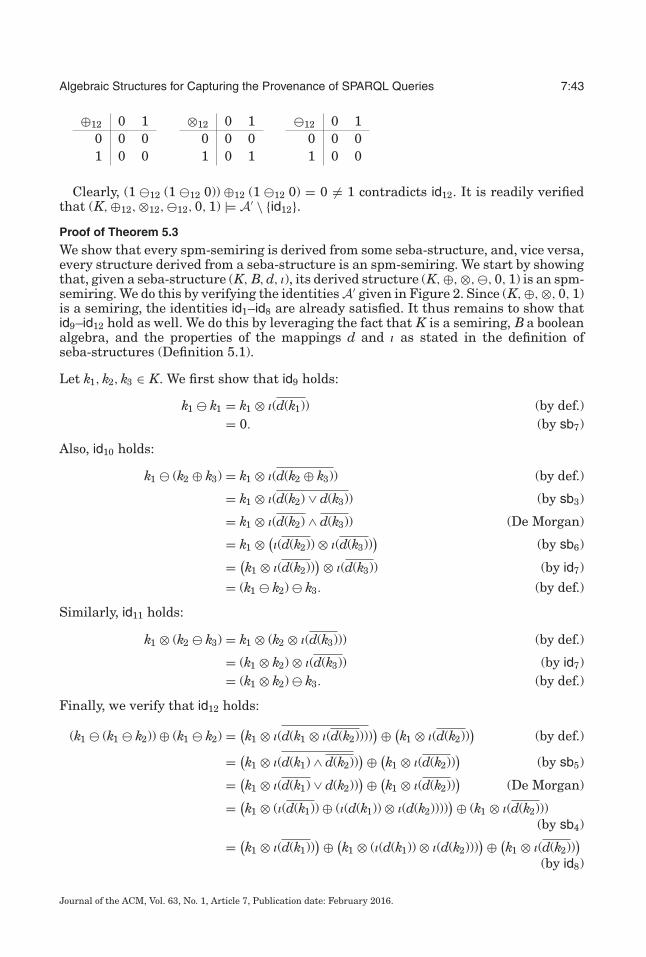
Algebraic Structures for Capturing the Provenance of SPARQL Queries 7:43
⊕12 0 10 0 01 0 0
⊗12 0 10 0 01 0 1
�12 0 10 0 01 0 0
Clearly, (1 �12 (1 �12 0)) ⊕12 (1 �12 0) = 0 �= 1 contradicts id12. It is readily verifiedthat (K,⊕12,⊗12,�12, 0, 1) |= A′ \ {id12}.Proof of Theorem 5.3
We show that every spm-semiring is derived from some seba-structure, and, vice versa,every structure derived from a seba-structure is an spm-semiring. We start by showingthat, given a seba-structure (K, B, d, ı), its derived structure (K,⊕,⊗,�, 0, 1) is an spm-semiring. We do this by verifying the identities A′ given in Figure 2. Since (K,⊕,⊗, 0, 1)is a semiring, the identities id1–id8 are already satisfied. It thus remains to show thatid9–id12 hold as well. We do this by leveraging the fact that K is a semiring, B a booleanalgebra, and the properties of the mappings d and ı as stated in the definition ofseba-structures (Definition 5.1).
Let k1, k2, k3 ∈ K. We first show that id9 holds:
k1 � k1 = k1 ⊗ ı(d(k1)) (by def.)= 0. (by sb7)
Also, id10 holds:
k1 � (k2 ⊕ k3) = k1 ⊗ ı(d(k2 ⊕ k3)) (by def.)
= k1 ⊗ ı(d(k2) ∨ d(k3)) (by sb3)
= k1 ⊗ ı(d(k2) ∧ d(k3)) (De Morgan)
= k1 ⊗ (ı(d(k2)) ⊗ ı(d(k3))
)(by sb6)
= (k1 ⊗ ı(d(k2))
)⊗ ı(d(k3)) (by id7)
= (k1 � k2) � k3. (by def.)
Similarly, id11 holds:
k1 ⊗ (k2 � k3) = k1 ⊗ (k2 ⊗ ı(d(k3))) (by def.)
= (k1 ⊗ k2) ⊗ ı(d(k3)) (by id7)= (k1 ⊗ k2) � k3. (by def.)
Finally, we verify that id12 holds:
(k1 � (k1 � k2)) ⊕ (k1 � k2) = (k1 ⊗ ı(d(k1 ⊗ ı(d(k2))))
)⊕ (k1 ⊗ ı(d(k2))
)(by def.)
= (k1 ⊗ ı(d(k1) ∧ d(k2))
)⊕ (k1 ⊗ ı(d(k2))
)(by sb5)
= (k1 ⊗ ı(d(k1) ∨ d(k2))
)⊕ (k1 ⊗ ı(d(k2))
)(De Morgan)
= (k1 ⊗ (ı(d(k1)) ⊕ (ı(d(k1)) ⊗ ı(d(k2))))
)⊕ (k1 ⊗ ı(d(k2)))(by sb4)
= (k1 ⊗ ı(d(k1))
)⊕ (k1 ⊗ (ı(d(k1)) ⊗ ı(d(k2)))
)⊕ (k1 ⊗ ı(d(k2))
)(by id8)
Journal of the ACM, Vol. 63, No. 1, Article 7, Publication date: February 2016.
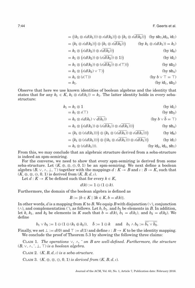
7:44 F. Geerts et al.
= ((k1 ⊗ ı(d(k1))) ⊗ ı(d(k2))
)⊕ (k1 ⊗ ı(d(k2))
)(by sb7,id3, id7)
= (k1 ⊗ ı(d(k2))
)⊕ (k1 ⊗ ı(d(k2))
)(by k1 ⊗ ı(d(k1)) = k1)
= k1 ⊗ (ı(d(k2)) ⊕ ı(d(k2))
)(by id8)
= k1 ⊗ (ı(d(k2)) ⊕ (ı(d(k2)) ⊗ 1)
)(by id1)
= k1 ⊗ (ı(d(k2)) ⊕ (ı(d(k2)) ⊗ ı(�))
)(by sb2)
= k1 ⊗ (ı(d(k2) ∨ �)
)(by sb4)
= k1 ⊗ (ı(�)) (by b ∨ � = �)= k1. (by id1, sb2)
Observe that here we use known identities of boolean algebras and the identity thatstates that for any k1 ∈ K, k1 ⊗ ı(d(k1)) = k1. The latter identity holds in every seba-structure:
k1 = k1 ⊗ 1 (by id1)= k1 ⊗ ı(�) (by sb2)
= k1 ⊗ ı(d(k1) ∨ d(k1)) (by b ∨ b = �)
= k1 ⊗ (ı(d(k1)) ⊕ (ı(d(k1)) ⊗ ı(d(k1)))
)(by sb4)
= (k1 ⊗ (ı(d(k1)))
)⊕ (k1 ⊗ (ı(d(k1)) ⊗ ı(d(k1)))
)(by id8)
= (k1 ⊗ (ı(d(k1)))
)⊕ ((k1 ⊗ ı(d(k1))) ⊗ ı(d(k1))
)(by id7)
= k1 ⊗ (ı(d(k1))). (by id2, id3, sb7)
From this, we may conclude that an algebraic structure derived from a seba-structureis indeed an spm-semiring.
For the converse, we need to show that every spm-semiring is derived from someseba-structure. Let (K,⊕,⊗,�, 0, 1) be an spm-semiring. We next define a booleanalgebra (B,∨,∧,⊥,�) together with the mappings d : K → B and ı : B → K, such that(K,⊕,⊗,�, 0, 1) is derived from (K, B, d, ı).
Let d : K → K be defined such that for every k ∈ K,
d(k) := 1 � (1 � k).
Furthermore, the domain of the boolean algebra is defined as
B := {b ∈ K | ∃k ∈ K, b = d(k)}.In other words, d is a mapping from K to B. We equip Bwith disjunction (∨), conjunction(∧), and complementation (¯), as follows. Let b, b1, and b2 be elements in B. In addition,let k, k1, and k2 be elements in K such that b = d(k), b1 = d(k1), and b2 = d(k2). Wedefine
b1 ∨ b2 := 1 � (1 � (k1 ⊕ k2)), b := 1 � k and b1 ∧ b2 := b1 ∨ b2.
Finally, we set ⊥ := d(0) and � := d(1) and define ı : B → K to be the identity mapping.We conclude the proof of Theorem 5.3 by showing the following three claims:
CLAIM 1. The operations ∨, ∧, ¯ on B are well-defined. Furthermore, the structure(B,∨,∧, ¯,⊥,�) is a boolean algebra.
CLAIM 2. (K, B, d, ı) is a seba-structure.
CLAIM 3. (K,⊕,⊗,�, 0, 1) is derived from (K, B, d, ı).
Journal of the ACM, Vol. 63, No. 1, Article 7, Publication date: February 2016.

Algebraic Structures for Capturing the Provenance of SPARQL Queries 7:45
Fig. 5. Identities used in the proof of Claims 1, 2, and 3.
It remains to verify the three claims, which we do next.We start by verifying that a number of identities, id13–id18, as shown in Figure 5,
are implied by the identities A′ that define spm-semirings. These auxilliary identitieswill be used extensively in the proofs of the three claims. Recall that, apart from theidentities in A′, we may also use id2 and id3 because these are already shown to beimplied by A′ in Proposition 4.6. We further observe that id13 is shown to be implied byA′ in Proposition 4.4.
The following derivations have been both manually verified and verified withProver9 [McCune 2010], which proves identities in equational logic, among otherthings.
We start by showing that A′ |= id14. This identity states that (k1 ⊕ k2) � k3 = (k1 � k3) ⊕(k2 � k3) for all k1, k2 and k3 in K.
(k1 ⊕ k2) � k3 = (k1 ⊕ k2) ⊗ (1 � k3) (by id1 and id11)= (k1 ⊗ (1 � k3)) ⊕ (k2 ⊗ (1 � k3)) (by id8)= (k1 � k3) ⊕ (k2 � k3). (by id1 and id11)
We also have that A′ |= id15, where id15 states that for all k1, k2, k3, and k4 in K,(k1 � k2) ⊗ (k3 � k4) = (k1 ⊗ k3) � (k2 ⊕ k4).
(k1 � k2) ⊗ (k3 � k4) = (k1 ⊗ (1 � k2)) ⊗ (k3 ⊗ (1 � k4)) (by id1 and id11)= (k1 ⊗ k3) ⊗ (1 � k2) ⊗ (1 � k4) (by id5 and id7)= (k1 ⊗ k3) ⊗ ((1 � k2) � k4) (by id1 and id11)= (k1 ⊗ k3) ⊗ (1 � (k2 ⊕ k4)) (by id10)= (k1 ⊗ k3) � (k2 ⊕ k4). (by id1 and id11)
We next verify that id16 is implied by A′. This identity states that for all k1, k2 ∈ K,k1 � (k1 � (k1 � k2)) = k1 � k2. To show that A′ |= id16, we assume that the followingadditional identities are shown to be implied by A′:
Journal of the ACM, Vol. 63, No. 1, Article 7, Publication date: February 2016.
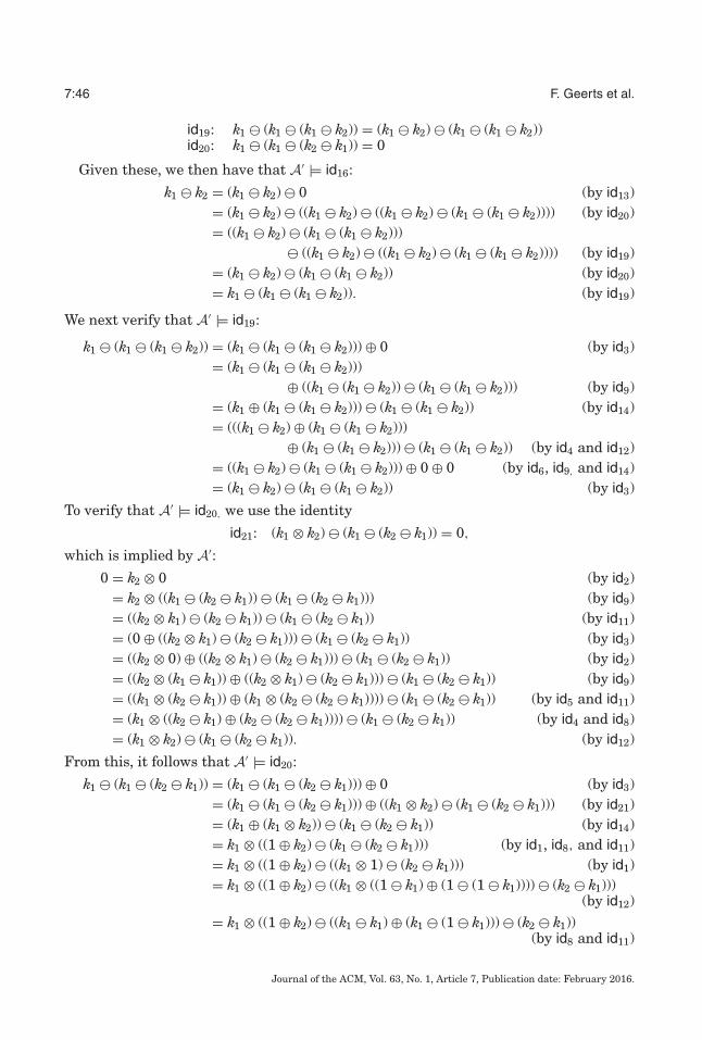
7:46 F. Geerts et al.
id19: k1 � (k1 � (k1 � k2)) = (k1 � k2) � (k1 � (k1 � k2))id20: k1 � (k1 � (k2 � k1)) = 0
Given these, we then have that A′ |= id16:
k1 � k2 = (k1 � k2) � 0 (by id13)= (k1 � k2) � ((k1 � k2) � ((k1 � k2) � (k1 � (k1 � k2)))) (by id20)= ((k1 � k2) � (k1 � (k1 � k2)))
� ((k1 � k2) � ((k1 � k2) � (k1 � (k1 � k2)))) (by id19)= (k1 � k2) � (k1 � (k1 � k2)) (by id20)= k1 � (k1 � (k1 � k2)). (by id19)
We next verify that A′ |= id19:
k1 � (k1 � (k1 � k2)) = (k1 � (k1 � (k1 � k2))) ⊕ 0 (by id3)= (k1 � (k1 � (k1 � k2)))
⊕ ((k1 � (k1 � k2)) � (k1 � (k1 � k2))) (by id9)= (k1 ⊕ (k1 � (k1 � k2))) � (k1 � (k1 � k2)) (by id14)= (((k1 � k2) ⊕ (k1 � (k1 � k2)))
⊕ (k1 � (k1 � k2))) � (k1 � (k1 � k2)) (by id4 and id12)= ((k1 � k2) � (k1 � (k1 � k2))) ⊕ 0 ⊕ 0 (by id6, id9, and id14)= (k1 � k2) � (k1 � (k1 � k2)) (by id3)
To verify that A′ |= id20, we use the identity
id21: (k1 ⊗ k2) � (k1 � (k2 � k1)) = 0,
which is implied by A′:
0 = k2 ⊗ 0 (by id2)= k2 ⊗ ((k1 � (k2 � k1)) � (k1 � (k2 � k1))) (by id9)= ((k2 ⊗ k1) � (k2 � k1)) � (k1 � (k2 � k1)) (by id11)= (0 ⊕ ((k2 ⊗ k1) � (k2 � k1))) � (k1 � (k2 � k1)) (by id3)= ((k2 ⊗ 0) ⊕ ((k2 ⊗ k1) � (k2 � k1))) � (k1 � (k2 � k1)) (by id2)= ((k2 ⊗ (k1 � k1)) ⊕ ((k2 ⊗ k1) � (k2 � k1))) � (k1 � (k2 � k1)) (by id9)= ((k1 ⊗ (k2 � k1)) ⊕ (k1 ⊗ (k2 � (k2 � k1)))) � (k1 � (k2 � k1)) (by id5 and id11)= (k1 ⊗ ((k2 � k1) ⊕ (k2 � (k2 � k1)))) � (k1 � (k2 � k1)) (by id4 and id8)= (k1 ⊗ k2) � (k1 � (k2 � k1)). (by id12)
From this, it follows that A′ |= id20:
k1 � (k1 � (k2 � k1)) = (k1 � (k1 � (k2 � k1))) ⊕ 0 (by id3)= (k1 � (k1 � (k2 � k1))) ⊕ ((k1 ⊗ k2) � (k1 � (k2 � k1))) (by id21)= (k1 ⊕ (k1 ⊗ k2)) � (k1 � (k2 � k1)) (by id14)= k1 ⊗ ((1 ⊕ k2) � (k1 � (k2 � k1))) (by id1, id8, and id11)= k1 ⊗ ((1 ⊕ k2) � ((k1 ⊗ 1) � (k2 � k1))) (by id1)= k1 ⊗ ((1 ⊕ k2) � ((k1 ⊗ ((1 � k1) ⊕ (1 � (1 � k1)))) � (k2 � k1)))
(by id12)= k1 ⊗ ((1 ⊕ k2) � ((k1 � k1) ⊕ (k1 � (1 � k1))) � (k2 � k1))
(by id8 and id11)
Journal of the ACM, Vol. 63, No. 1, Article 7, Publication date: February 2016.

Algebraic Structures for Capturing the Provenance of SPARQL Queries 7:47
= k1 ⊗ ((1 ⊕ k2) � (0 ⊕ (k1 � (1 � k1))) � (k2 � k1)) (by id9)= k1 ⊗ ((1 ⊕ k2) � ((k1 � (1 � k1)) � (k2 � k1))) (by id3)= k1 ⊗ ((1 ⊕ k2) � (k1 � ((1 � k1) ⊕ (k2 � k1)))) (by id10)= k1 ⊗ ((1 ⊕ k2) � (k1 � ((1 ⊕ k2) � k1))) (by id14)= (k1 ⊗ (1 ⊕ k2)) � (k1 � ((1 ⊕ k2) � k1)) (by id11)= 0. (by id21)
We next consider id17, which states that (k1 � k2) � (1 � k3) = k1 � (1 � (k3 � k2)) for allk1, k2 and k3 in K. To verify that A′ |= id17, we need the following auxiliary identities:
id22: k1 � (1 � k2) = k1 � (k1 � k2)id23: (k1 � k2) � (k3 � k2) = (k1 � k2) � k3id24: k1 � (1 � (k3 � k2)) = (k1 � k2) � (1 � (k3 � k2))
Indeed, given these, we have that
(k1 � k2) � (1 � k3) = (k1 � k2) � ((k1 � k2) � k3) (by id22)= (k1 � k2) � ((k1 � k2) � (k3 � k2)) (by id23)= (k1 � k2) � (1 � (k3 � k2)) (by id22)= k1 � (1 � (k3 � k2)). (by id24)
It remains to verify that id22, id23, and id24 are implied by A′. We start by verifyingA′ |= id22:
k1 � (1 � k2) = k1 ⊗ (1 � (1 � k2)) (by id11)= (1 � (1 � k2)) ⊗ k1 (by id5)= (1 � (1 � k2)) ⊗ ((k1 � (1 � (1 � k2)))
⊕ (k1 � (k1 � (1 � (1 � k2))))) (by id4 and id12)= ((1 � (1 � k2)) ⊗ (k1 � (1 � (1 � k2))))
⊕ ((1 � (1 � k2)) ⊗ (k1 � (k1 � (1 � (1 � k2))))) (by id8)= (k1 ⊗ ((1 � (1 � k2)) � (1 � (1 � k2))))
⊕ ((1 � (1 � k2)) ⊗ (k1 � (k1 � (1 � (1 � k2))))) (by id4 and id11)= 0 ⊕ ((1 � (1 � k2)) ⊗ (k1 � (k1 � (1 � (1 � k2))))) (by id2 and id9)= (k1 ⊗ (1 � (1 � k2))) � (k1 � (1 � (1 � k2))) (by id3, id5, and id11)= (k1 ⊗ (1 � (1 � k2))) � (k1 ⊗ (1 � (1 � (1 � k2)))) (by id1 and id11)= (k1 ⊗ (1 � (1 � k2))) � (k1 � k2) (by id1, id11, and id16)= 0 ⊕ ((k1 ⊗ (1 � (1 � k2))) � (k1 � k2)) (by id3)= ((k1 � k2) � (k1 � k2)) ⊕ ((k1 ⊗ (1 � (1 � k2))) � (k1 � k2)) (by id9)= ((k1 � k2) ⊕ (k1 � (1 � k2))) � (k1 � k2) (by id11 and id14)= (k1 ⊗ ((1 � k2) ⊕ (1 � (1 � k2)))) � (k1 � k2) (by id8 and id11)= (k1 ⊗ 1) � (k1 � k2) (by id4 and id12)= k1 � (k1 � k2). (by id11)
Journal of the ACM, Vol. 63, No. 1, Article 7, Publication date: February 2016.

7:48 F. Geerts et al.
To show A′ |= id23, we proceed as follows. Assume that
id25: k1 � (k2 � k1) = k1id26: k1 � (k2 � (k3 � k1)) = k1 � k2
is implied by A′. Then,
(k1 � k2) � k3 = (k1 � k2) � (k3 � (k2 � (k1 � k2))) (by id26)= (k1 � k2) � ((k3 � (k2 � (k1 � k2))) � 0) (by id13)= (k1 � k2) � ((k3 � (k2 � (k1 � k2))) � (k2 � (k2 � (k1 � k2)))) (by id20)= (k1 � k2) � (k3 � ((k2 � (k1 � k2)) ⊕ (k2 � (k2 � (k1 � k2))))) (by id10)= (k1 � k2) � (k3 � k2). (by id4 and id12)
The identity id25 is indeed implied by A′:
k1 = (k1 � (k2 � k1)) ⊕ (k1 � (k1 � (k2 � k1))) (by id4 and id12)= (k1 � (k2 � k1)). (by id3 and id20)
The same holds for the identity id26:
k1 � k2 = k1 � ((k2 � (1 � (k3 � k1))) ⊕ (k2 � (k2 � (1 � (k3 � k1))))) (by id4 and id12)= (k1 � (k2 � (1 � (k3 � k1)))) � (k2 � (k2 � (1 � (k3 � k1)))) (by id10)= (((k1 � (k3 � k1)) ⊕ (k1 � (k1 � (k3 � k1))))
� (k2 � (1 � (k3 � k1)))) � (k2 � (k2 � (1 � (k3 � k1)))) (by id4 and id12)= (((k1 � (k3 � k1)) ⊕ 0) � (k2 � (1 � (k3 � k1))))
� (k2 � (k2 � (1 � (k3 � k1)))) (by id20)= ((k1 � (k3 � k1)) � (k2 � (1 � (k3 � k1))))
� (k2 � (k2 � (1 � (k3 � k1)))) (by id3)= (k1 ⊗ ((1 � (k3 � k1)) � (k2 � (1 � (k3 � k1)))))
� (k2 � (k2 � (1 � (k3 � k1)))) (by id1 and id11)= (k1 ⊗ (1 � (k3 � k1))) � (k2 � (k2 � (1 � (k3 � k1)))) (by id25)= (k1 � (k3 � k1)) � (k2 � (k2 � (1 � (k3 � k1)))) (by id1 and id11)= k1 � (k2 � (k2 � (1 � (k3 � k1)))) (by id25)= k1 � (k2 � (k2 � (k2 � (k3 � k1)))) (by id22)= k1 � (k2 � (k3 � k1)). (by id16)
We next show that A′ |= id24, which states that (k1 � k2) � (1 � (k3 � k2)) = k1 � (1 �(k3 � k2)) for all k1, k2, and k3 in K. Assume that
id27: k1 � (k2 � (1 � (k3 � k1))) = k1
is implied by A′. Then, A′ |= id24:
(k1 � k2) � (1 � (k3 � k2)) = (k1 � (k2 � (1 � k2))) � (1 � (k3 � k2)) (by id25)= (k1� (k2� (1 � (k2 � (k1� (1 � (k3� k2))))))) � (1 � (k3� k2))
(by id27)= (k1 � (1 � (k3 � k2))) � (k2� (1 � (k2� (k1� (1� (k3� k2))))))
(by id4 and id10)= k1 � (1 � (k3 � k2)). (by id27)
Journal of the ACM, Vol. 63, No. 1, Article 7, Publication date: February 2016.

Algebraic Structures for Capturing the Provenance of SPARQL Queries 7:49
The identity id27 is indeed implied by A′:
k1 = k1 � (k3 � k1) (by id25)= k1 ⊗ (1 � (k3 � k1)) (by id11)= k1 ⊗ ((1 � (k3 � k1)) � (k2 � (1 � (k3 � k1)))) (by id25)= (k1 � (k3 � k1)) � (k2 � (1 � (k3 � k1))) (by id11)= k1 � (k2 � (1 � (k3 � k1))) (by id25)
Finally, we verify that A′ implies id18, which states that k1 � (k2 ⊕ k2) = k1 � k2 for allk1, k2 in K.
k1 � k2 = (k1 � k2) ⊗ 1 (by id1)= (k1 � k2) ⊗ ((1 � k2) ⊕ (1 � (1 � k2))) (by id4 and id12)= ((k1 � k2) � k2) ⊕ ((k1 � k2) � (1 � k2)) (by id1, id8, and id11)= ((k1 � k2) � k2) ⊕ (k1 � (k2 ⊕ (1 � k2))) (by id10)= ((k1 � k2) � k2) ⊕ (k1 ⊗ (1 � (k2 ⊕ (1 � k2))))
(by id1 and id11)= ((k1 � k2) � k2) ⊕ (k1 ⊗ ((1 � k2) � (1 � k2))) (by id10)= ((k1 � k2) � k2) ⊕ (k1 ⊗ 0) (by id9)= k1 � (k2 ⊕ k2). (by id2, id3, and id10)
Hence, A′ |= {id1, . . . , id18}. We are now ready to prove the three claims.
PROOF OF CLAIM 1. We first check whether the definitions of disjunction, conjunction,and complementation are independent of the choice of elements in K and thus thatthese operations are well-defined. Since conjunction is defined in terms of disjunctionand complementation, it suffices to consider disjunction and complementation only. Letk, k1, k2, , 1, and 2 be elements in K such that b = d(k) = d(), b1 = d(k1) = d(1), andb2 = d(k2) = d(2). We start by showing that complementation is well-defined:
b := 1 � k (by def.)= 1 � (1 � (1 � k)) (by id16)= 1 � (1 � (1 � )) (by d(k) = d())= 1 � . (by id16)
For disjunction, we observe the following:
b1 ∨ b2 := 1 � (1 � (k1 ⊕ k2)) (by def.)= 1 � ((1 � k1) � k2) (by id10)= 1 � ((1 � 1) � k2) (by d(k) = d())= 1 � (1 � (1 ⊕ k2)) (by id10)= 1 � (1 � (k2 ⊕ 1)) (by id4)= 1 � ((1 � k2) � 1) (by id10)= 1 � ((1 � 2) � 1) (by d(k) = d())= 1 � (1 � (2 ⊕ 1)) (by id10)= 1 � (1 � (1 ⊕ 2)). (by id4)
Hence, ¯ and ∨ are well-defined and so is ∧.
Journal of the ACM, Vol. 63, No. 1, Article 7, Publication date: February 2016.

7:50 F. Geerts et al.
Fig. 6. Axiomatization of Boolean algebras.
We next verify that (B,∨,∧, ¯,⊥,�) is indeed a Boolean algebra. We do this by showingthat this structure satisfies the three identities b1, b2, and b3 (the “fourth set” ofpostulates, [Huntington 1933b, page 280] and corrected in Huntington [1933a]) shownin Figure 6. The commutativity (b1) of the disjunction (∨) follows immediately from thedefinition of disjunction and the fact that ⊕ is commutative (id4). For associativity (b2),we observe the following. Let b1, b2, and b3 in B and k1, k2, and k3 in K be such thatbi = d(ki), for i = 1, 2, 3.
b1 ∨ (b2 ∨ b3) := 1 � (1 � (k1 ⊕ (1 � (1 � (k2 ⊕ k3))))) (by def.)= 1 � ((1 � k1) � (1 � (1 � (k2 ⊕ k3)))) (by id10)= 1 � ((1 � k1) ⊗ (1 � (1 � (1 � (k2 ⊕ k3))))) (by id1 and id11)= 1 � ((1 � k1) ⊗ (1 � (k2 ⊕ k3))) (by id16)= 1 � ((1 � k1) � (k2 ⊕ k3)) (by id1 and id11)= 1 � (1 � (k1 ⊕ (k2 ⊕ k3))) (by id10)= 1 � (1 � ((k1 ⊕ k2) ⊕ k3)) (by id6)= 1 � ((1 � k3) � (k1 ⊕ k2)) (by id4 and id10)= 1 � ((1 � k3) ⊗ (1 � (k1 ⊕ k2))) (by id1 and id11)= 1 � ((1 � k3) ⊗ (1 � (1 � (1 � (k1 ⊕ k2))))) (by id16)= 1 � ((1 � k3) � (1 � (1 � (k1 ⊕ k2)))) (by id1 and id11)= 1 � (1 � ((1 � (1 � (k1 ⊕ k2))) ⊕ k3)) (by id4 and id10):= (b1 ∨ b2) ∨ b3 (by def.)
It remains to verify (b3). Let k1, k2 ∈ K and b1, b2 ∈ Bsuch that b1 = d(k1) and b2 = d(k2).Recall that, by definition, b1 ∧ b2 := (b1 ∨ b2) ∨ (b1 ∨ b2). Let us first consider (b1 ∨ b2)and b1 ∨ b2.
(b1 ∨ b2) = 1 � (1 � (1 � ((1 � (1 � (1 � k1))) ⊕ (1 � (1 � (1 � k2)))))) (by def.)= 1 � (1 � (1 � ((1 � k1) ⊕ (1 � k2)))) (by id16)= 1 � ((1 � k1) ⊕ (1 � k2)), (by id16)
and similarly,
b1 ∨ b2 = 1 � ((1 � k1) ⊕ (1 � (1 � k2))).
Hence, (b1 ∨ b2) ∨ (b1 ∨ b2) is equal to
1 � (1 � ((1 � ((1 � k1) ⊕ (1 � k2))) ⊕ (1 � ((1 � k1) ⊕ (1 � (1 � k2)))))) (by def.)= 1 � (1 � (((1 � (1 � k2)) � (1 � k1)) ⊕ ((1 � (1 � (1 � k2))) � (1 � k1))))
(by id4 and id10)= 1 � (1 � (((1 � (1 � k2)) � (1 � k1)) ⊕ ((1 � k2) � (1 � k1)))) (by id16)= 1 � (1 � ((((1 � (1 � k2)) ⊕ (1 � k2)) � (1 � k1)))) (by id14)
Journal of the ACM, Vol. 63, No. 1, Article 7, Publication date: February 2016.

Algebraic Structures for Capturing the Provenance of SPARQL Queries 7:51
= 1 � (1 � (1 � (1 � k1))) (by id12)= 1 � (1 � k1), (by id16)
which in turn is equal to b1.Hence, ∨ and ¯ satisfy b1–b3. It has been shown in Huntington [1933b] that when ∧
is defined in terms of ∨ and ¯, as we do, then � is uniquely determined by � = b ∨ b.In addition, ⊥ := �. It is known that these operations and constants define a Booleanalgebra [Huntington 1933b]. Since we defined � := d(1) and ⊥ := d(0), it remains to beshown that d(1) = b ∨ b for any b ∈ B and that d(0) = d(1). Observe the following: Letb ∈ B and k ∈ K such that b = d(k). Then,
b ∨ b := 1 � (1 � (k ⊕ (1 � k))) (by def.)= 1 � ((1 � k) � (1 � k)) (by id10)= 1 � 0 (by id9)= 1 � (1 � 1) (by id9)= d(1) (by def.)
Furthermore, d(1) = 1 � (1 � (1 � 1)) = 1 � (1 � 0) = d(0) by id9 and the definitionof d. Hence, we may conclude that (B,∨,∧, ¯,⊥,�) is indeed a boolean algebra. Thisconcludes the proof of Claim 1.
PROOF OF CLAIM 2. We need to verify that (K, B, d, ı) satisfies sb1–sb7.Since we defined ⊥ := d(0) and � := d(1), sb1 is automatically satisfied. For sb2, we
observe that ı(⊥) = ı(d(0)) = d(0) = 0 and ı(�) = ı(d(1)) = d(1) = 1. This follows fromthe definition of d and ı, and identities id9 and id13.
We next show that sb3 holds; that is, for any k, ∈ K, d(k ⊕ ) = d(k) ∨ d(). Observethat d(k⊕ ) = 1 � (1 � (k⊕ )) which is equal to d(k) ∨ d() by the definition of d and ∨.
We verify sb5; that is, for any k ∈ K, b ∈ B, d(k⊗ ı(b)) = d(k) ∧ b, as follows. Let ∈ Kbe such that b = d(). Then,
d(k ⊗ (1 � (1 � ))) = 1 � (1 � (k ⊗ (1 � (1 � )))) (by def.)= 1 � (1 � (k � (1 � )))) (by id1 and id11)= (1 � (1 � )) � (1 � k) (by id17)= 1 � ((1 � k) ⊕ (1 � )) (by id4 and id10)
= d(k) ∨ d() (by id16 and def.)= d(k) ∧ b. (by def.)
For sb4, we need to show that for any b, b′ ∈ B, ı(b ∨ b′) = ı(b) ⊕ (ı(b) ⊗ ı(b′)). Since, ı isthe identity mapping, this is equivalent to showing that for any k, ∈ K, d(k) ∨ d() =d(k) ⊕ (d(k) ⊗ d()).
d(k) ∨ d() = 1 � (1 � (k ⊕ )) (by def.)= 1 � ((1 � k) ⊗ (1 � )) (by id15)= ((1 � k) ⊕ (1 � (1 � k))) � ((1 � k) ⊗ (1 � )) (by id12)= ((1 � k) � ((1 � k) ⊗ (1 � ))) ⊕ ((1 � (1 � k)) � ((1 � k) ⊗ (1 � )))
(by id14)= ((1 � k) � (1 � )) ⊕ ((1 � (1 � k)) � ((1 � k) ⊗ (1 � ))) (by id16)= ((1 � (k ⊕ (1 � )))) ⊕ ((1 � (1 � k)) � ((1 � k) ⊗ (1 � )))
(by id1, id11, and id12)
Journal of the ACM, Vol. 63, No. 1, Article 7, Publication date: February 2016.
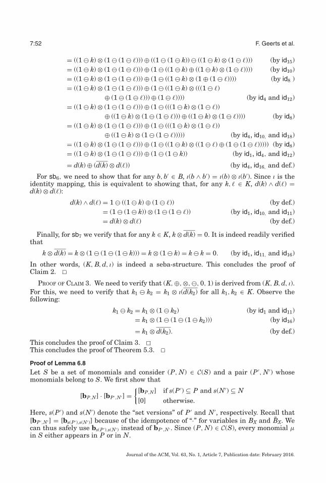
7:52 F. Geerts et al.
= ((1 � k) ⊗ (1 � (1 � ))) ⊕ ((1 � (1 � k)) � ((1 � k) ⊗ (1 � ))) (by id15)= ((1 � k) ⊗ (1 � (1 � ))) ⊕ (1 � ((1 � k) ⊕ ((1 � k) ⊗ (1 � )))) (by id10)= ((1 � k) ⊗ (1 � (1 � ))) ⊕ (1 � ((1 � k) ⊗ (1 ⊕ (1 � )))) (by id8 )= ((1 � k) ⊗ (1 � (1 � ))) ⊕ (1 � ((1 � k) ⊗ (((1 � )
⊕ (1 � (1 � ))) ⊕ (1 � )))) (by id4 and id12)= ((1 � k) ⊗ (1 � (1 � ))) ⊕ (1 � (((1 � k) ⊗ (1 � ))
⊕ ((1 � k) ⊗ (1 � (1 � ))) ⊕ ((1 � k) ⊗ (1 � )))) (by id8)= ((1 � k) ⊗ (1 � (1 � ))) ⊕ (1 � (((1 � k) ⊗ (1 � ))
⊕ ((1 � k) ⊗ (1 � (1 � ))))) (by id4, id10, and id18)= ((1 � k) ⊗ (1 � (1 � ))) ⊕ (1 � ((1 � k) ⊗ ((1 � ) ⊕ (1 � (1 � ))))) (by id8)= ((1 � k) ⊗ (1 � (1 � ))) ⊕ (1 � (1 � k)) (by id1, id4, and id12)
= d(k) ⊕ (d(k) ⊗ d()) (by id4, id16, and def.)
For sb6, we need to show that for any b, b′ ∈ B, ı(b ∧ b′) = ı(b) ⊗ ı(b′). Since ı is theidentity mapping, this is equivalent to showing that, for any k, ∈ K, d(k) ∧ d() =d(k) ⊗ d():
d(k) ∧ d() = 1 � ((1 � k) ⊕ (1 � )) (by def.)= (1 � (1 � k)) ⊗ (1 � (1 � )) (by id1, id10, and id11)= d(k) ⊗ d() (by def.)
Finally, for sb7 we verify that for any k ∈ K, k⊗ d(k) = 0. It is indeed readily verifiedthat
k ⊗ d(k) = k ⊗ (1 � (1 � (1 � k))) = k ⊗ (1 � k) = k � k = 0. (by id1, id11, and id16)
In other words, (K, B, d, ı) is indeed a seba-structure. This concludes the proof ofClaim 2.
PROOF OF CLAIM 3. We need to verify that (K,⊕,⊗,�, 0, 1) is derived from (K, B, d, ı).For this, we need to verify that k1 � k2 = k1 ⊗ ı(d(k2) for all k1, k2 ∈ K. Observe thefollowing:
k1 � k2 = k1 ⊗ (1 � k2) (by id1 and id11)= k1 ⊗ (1 � (1 � (1 � k2))) (by id16)
= k1 ⊗ d(k2). (by def.)
This concludes the proof of Claim 3.This concludes the proof of Theorem 5.3.
Proof of Lemma 6.8
Let S be a set of monomials and consider (P, N) ∈ C(S) and a pair (P ′, N′) whosemonomials belong to S. We first show that
[bP,N] · [bP ′,N′ ] ={
[bP,N] if s(P ′) ⊆ P and s(N′) ⊆ N[0] otherwise.
Here, s(P ′) and s(N′) denote the “set versions” of P ′ and N′, respectively. Recall that[bP ′,N′ ] = [bs(P ′),s(N′)] because of the idempotence of “·” for variables in BX and BX. Wecan thus safely use bs(P ′),s(N′) instead of bP ′,N′ . Since (P, N) ∈ C(S), every monomial μin S either appears in P or in N.
Journal of the ACM, Vol. 63, No. 1, Article 7, Publication date: February 2016.
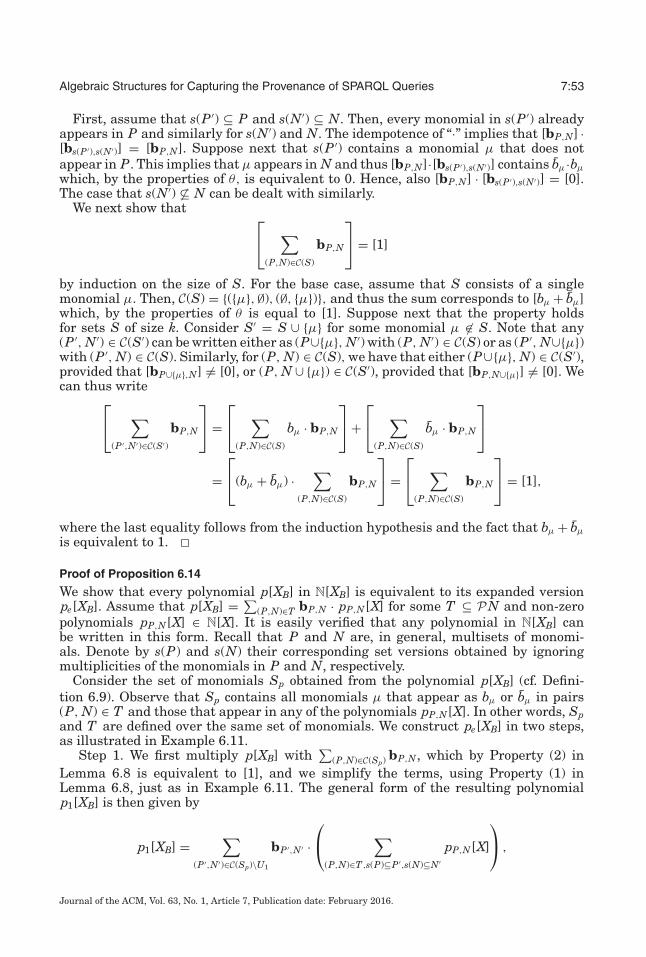
Algebraic Structures for Capturing the Provenance of SPARQL Queries 7:53
First, assume that s(P ′) ⊆ P and s(N′) ⊆ N. Then, every monomial in s(P ′) alreadyappears in P and similarly for s(N′) and N. The idempotence of “·” implies that [bP,N] ·[bs(P ′),s(N′)] = [bP,N]. Suppose next that s(P ′) contains a monomial μ that does notappear in P. This implies that μ appears in N and thus [bP,N]·[bs(P ′),s(N′)] contains bμ ·bμ
which, by the properties of θ, is equivalent to 0. Hence, also [bP,N] · [bs(P ′),s(N′)] = [0].The case that s(N′) �⊆ N can be dealt with similarly.
We next show that ⎡⎣ ∑
(P,N)∈C(S)
bP,N
⎤⎦ = [1]
by induction on the size of S. For the base case, assume that S consists of a singlemonomial μ. Then, C(S) = {({μ},∅), (∅, {μ})}, and thus the sum corresponds to [bμ + bμ]which, by the properties of θ is equal to [1]. Suppose next that the property holdsfor sets S of size k. Consider S′ = S ∪ {μ} for some monomial μ �∈ S. Note that any(P ′, N′) ∈ C(S′) can be written either as (P∪{μ}, N′) with (P, N′) ∈ C(S) or as (P ′, N∪{μ})with (P ′, N) ∈ C(S). Similarly, for (P, N) ∈ C(S), we have that either (P∪{μ}, N) ∈ C(S′),provided that [bP∪{μ},N] �= [0], or (P, N ∪ {μ}) ∈ C(S′), provided that [bP,N∪{μ}] �= [0]. Wecan thus write⎡
⎣ ∑(P ′,N′)∈C(S′)
bP,N
⎤⎦ =
⎡⎣ ∑
(P,N)∈C(S)
bμ · bP,N
⎤⎦+
⎡⎣ ∑
(P,N)∈C(S)
bμ · bP,N
⎤⎦
=⎡⎣(bμ + bμ) ·
∑(P,N)∈C(S)
bP,N
⎤⎦ =
⎡⎣ ∑
(P,N)∈C(S)
bP,N
⎤⎦ = [1],
where the last equality follows from the induction hypothesis and the fact that bμ + bμ
is equivalent to 1.
Proof of Proposition 6.14
We show that every polynomial p[XB] in N[XB] is equivalent to its expanded versionpe[XB]. Assume that p[XB] = ∑
(P,N)∈T bP,N · pP,N[X] for some T ⊆ PN and non-zeropolynomials pP,N[X] ∈ N[X]. It is easily verified that any polynomial in N[XB] canbe written in this form. Recall that P and N are, in general, multisets of monomi-als. Denote by s(P) and s(N) their corresponding set versions obtained by ignoringmultiplicities of the monomials in P and N, respectively.
Consider the set of monomials Sp obtained from the polynomial p[XB] (cf. Defini-tion 6.9). Observe that Sp contains all monomials μ that appear as bμ or bμ in pairs(P, N) ∈ T and those that appear in any of the polynomials pP,N[X]. In other words, Spand T are defined over the same set of monomials. We construct pe[XB] in two steps,as illustrated in Example 6.11.
Step 1. We first multiply p[XB] with∑
(P,N)∈C(Sp) bP,N, which by Property (2) inLemma 6.8 is equivalent to [1], and we simplify the terms, using Property (1) inLemma 6.8, just as in Example 6.11. The general form of the resulting polynomialp1[XB] is then given by
p1[XB] =∑
(P ′,N′)∈C(Sp)\U1
bP ′,N′ ·⎛⎝ ∑
(P,N)∈T ,s(P)⊆P ′,s(N)⊆N′pP,N[X]
⎞⎠ ,
Journal of the ACM, Vol. 63, No. 1, Article 7, Publication date: February 2016.
7:54 F. Geerts et al.
where U1 denotes the set of pairs (P ′, N′) ∈ C(Sp) for which {(P, N) ∈ T , s(P) ⊆P ′, s(N) ⊆ N′} is empty. In terms of equivalence classes, it is safe to eliminate the termscorresponding to U1 because these are equivalent to 0 by Property (1) in Lemma 6.8.
Step 2. Next, for (P ′, N′) ∈ C(Sp) \ U1, denote by p′P,N[X] the polynomial in N[X]
obtained by removing all monomials μ from pP,N[X] such that μ ∈ N. If no monomialsare left in p′
P,N[X], we treat it as the zero polynomial. Furthermore, let rP ′,N′ [X] =∑(P,N)∈T ,s(P)⊆P ′,s(N)⊆N′ p′
P,N[X]. We can then write p1[XB] equivalently as
pe[XB] =∑
(P ′,N′)∈C(Sp)\(U1∪U2)
bP ′,N′ · rP ′,N′[X],
where U2 ⊆ C(Sp) \ U1 consists of all (P ′, N′) for which rP ′,N′[X] = 0. In terms ofequivalence classes, it is safe to eliminate the terms corresponding to U2 because thiscorresponds to the application of [bμ] · [μ] = [0].
We next verify that pe[XB] is the expanded version of p[XB] as defined in Defini-tion 6.15. For this, we need to show that (i) the polynomials rP ′,N′ [X] are non-zero anddo not contain monomials that occur in N′, and (ii) C(Sp) \ (U1U2) = Sp-supp(p[XB]).
Clearly, (i) follows from the construction of pe[XB]. We next verify (ii).We first show that Sp-supp(p[XB]) ⊆ C(Sp)\ (U1 ∪U2). Let (P, N) ∈ C(Sp) and assume
that (P, N) ∈ Sp-supp(p[XB]) but (P, N) ∈ U1 ∪U2. This is impossible, however. Indeed,(P, N) ∈ Sp-supp(p[XB]) implies that [0] �= [bP,N · p[XB]] = [bP,N · pe[XB]]. On the otherhand, (P, N) ∈ (U1 ∪ U2) implies that [bP,N · pe[XB]] = [0].
To show that C(Sp) \ (U1 ∪ U2) ⊆ Sp-supp(p[XB]), let (P ′, N′) ∈ C(Sp) \ (U1 ∪ U2)and assume that (P ′, N′) �∈ Sp-supp(p[XB]). The latter implies that [bP ′,N′ · p[XB]] =[0], and (P ′, N′) ∈ C(Sp) \ (U1 ∪ U2) implies that there exists a non-zero polynomialrP ′,N′[X] in pe[XB]. Hence, [bP ′,N′ · rP ′,N′[X]] = [0] and there must be a μ in rP ′,N′ [X] thatbelongs to N′. This contradicts the assumption that (P ′, N′) ∈ C(Sp) \ (U1 ∪ U2). Wemay thus conclude that C(Sp) \ (U1 ∪ U2) ⊆ Sp-supp(p[XB]). Hence, C(Sp) \ (U1 ∪ U2) =Sp-supp(p[XB]).
We conclude by showing that pe[XB] is uniquely determined by p[XB]. Let p′[XB] =∑(P ′,N′)∈Sp-supp(p[XB]) bP ′,N′ · sP ′,N′ [X] for some non-zero sP ′,N′ [X] ∈ N[X] none of whose
monomials appears in N′. Assume that (a) [p[XB]] = [p′[XB]] and (b) pe[XB] �= p′[XB]where pe[XB] is of the form (‡). From (a) we know that [pe[XB]] = [p′[XB]] and that[bP ′,N′ · pe[XB]] = [bP ′,N′ · rP ′,N′ [X]] = [bP ′,N′ · sP ′,N′[X]] = [bP ′,N′ · p′[XB]]. From (b), weknow that there is a pair (P ′, N′) in Sp-supp(p[XB]) such that rP ′,N′ [X] �= sP ′,N′[X].More specifically, let rP ′,N′ [X] = ∑
μ rμ · μ and sP ′,N′[X] = ∑μ sμ · μ and let μ be such
that rμ �= sμ. Without loss of generality, we may assume that sμ > rμ. To ensure that[bP ′,N′ · rP ′,N′ [X]] = [bP ′,N′ · sP ′,N′[X]], we thus must be able to go from bP ′,N′ · rP ′,N′[X] tobP ′,N′ · sP ′,N′ [X] by applying a sequence of rules (i)–(iv) as given in the definition of θ . Inparticular, we must add bP ′,N′ · (rμ − sμ) · μ to bP ′,N′ · rP ′,N′[X] to obtain bP ′,N′ · sP ′,N′[X].From the definition of θ , however, we can only introduce such a term using rule (iii).That is, whenever μ ∈ N. This is impossible since sP ′,N′ [X] is such that none of itsmonomials occurs in N′. Hence, [bP ′,N′ · rP ′,N′ [X]] �= [bP ′,N′ · sP ′,N′[X]], which contradicts(i). Hence, pe[XB] must be equal to p′[XB].
Proof of Proposition 6.16
Suppose that [p[XB]] = [q[XB]]. Recall that this implies that S-supp(p[XB]) =S-supp(q[XB]) for any S ⊆ mon(X). This holds in particular for S = Sp ∪ Sq.Furthermore, along the same lines as the proof of Proposition 6.14, one can show
Journal of the ACM, Vol. 63, No. 1, Article 7, Publication date: February 2016.

Algebraic Structures for Capturing the Provenance of SPARQL Queries 7:55
that
[pe[XB]] =⎡⎣ ∑
(P,N)∈(Sp ∪ Sq)-supp(p[XB])
bP,N · rP|Sp ,N|Sp[X]
⎤⎦
[qe[XB]] =⎡⎣ ∑
(P,N)∈(Sp ∪ Sq)-supp(p[XB])
bP,N · sP|Sq ,N|Sq[X]
⎤⎦ ,
and that rP|Sp ,N|Sp[X] = sP|Sq ,N|Sq
[X] for any (P, N) ∈ (Sp ∪ Sq)-supp(p[XB]). Conversely,assume that rP|Sp ,N|Sp
[X] = sP|Sq ,N|Sq[X] for any (P, N) ∈ (Sp ∪ Sq)-supp(p[XB]). Then,
clearly, [pe[XB]] = [qe[XB]] and thus [p[XB]] = [q[XB]] by Proposition 6.14.
Proof of Proposition 6.18
We show that deciding equivalence of two polynomials in N[XB] is coNP-complete.Let p[XB] = ∑
(P,N)∈T bP,N · pP,N[X] and q[XB] = ∑(P,N)∈T ′ bP,N · qP,N[X] for some
T , T ′ ⊆ PN and non-zero polynomials pP,N[X] and qP,N[X] in N[X]. Let S = Sp∪Sq. Thefollowing algorithm decides the complement problem (i.e., whether [p[XB]] �= [q[XB]]holds):
(1) Guess an element (P, N) ∈ C(S). Denote by bP,N the corresponding monomial.(2) Verify the following:
(a) Compute p′[XB] = bP,N · p[XB] and q′[XB] = bP,N · q[XB].(b) Simplify p′[XB] and q′[XB] such that they are of the form bP,N ·r[X] and bP,N ·s[X]
in which neither r[X] nor s[X] contains monomials μ that occur in N.(c) Check whether r[X] �= s[X]. If so, return “yes.”
Clearly, the algorithm is in NP. Indeed, in Step (1) we can guess elements (P, N)from C(S) since their sizes are bounded by a polynomial in |S|. Furthermore, Step (2)is in PTIME. Indeed, it involves the PTIME computation of a product of polynomials(Step (2.a)), a PTIME simplification procedure (Step (2.b)) as given in the proof ofPropositon 6.14, and a simple equality check (Step (2.c)). The algorithm is to findtwo terms in the expanded versions of p[XB] and q[XB] for which the condition inProposition 6.16 is not satisfied, and hence these terms witness the fact that p[XB]and q[XB] are not equivalent. The correctness of the algorithm is thus immediate fromProposition 6.16. We may conclude that deciding whether [p[XB]] = [q[XB]] holds is incoNP.
For the lower bound, we prove the coNP-hardness by reduction from the tautologyproblem. An instance of the latter problem is φ = C1 ∨ · · · ∨ Cn, where all the variablesin φ are x1, . . . , xk, Cj is of the form lj1 ∧ lj2 ∧ lj3 , and li j is either xs or xs, s ∈ [1, k]. Theproblem is to determine whether all truth assignments make φ true. This problem isknown to be coNP-complete (cf. Garey and Johnson [1979]).
Given an instance φ, we define a polynomial pφ[X, BX, BX] with X = {x1, . . . , xk} suchthat [pφ[XB]] = [1] if and only if φ is a tautology. The polynomial pφ[XB] consists of nterms pCi , one for each clause Ci in φ, where pCi is the product of three variables inBX ∪ BX corresponding to the literals in the corresponding clause. That is, if in clause Ci, ji is a variable in xm ∈ X, then we put bxm in the product; if ji is a negated variable xm,for xm ∈ X, then we put bxm in the product. For example, if φ = (x1 ∧x2 ∧x3)∨(x1 ∧ x2 ∧x4),then pφ = bx1 · bx2 · bx3 + bx1 · bx2 · bx4 . We claim that [pφ[XB]] = [1] iff φ is a tautology.
Consider a truth assignment τ : X → {0, 1}. We associate with τ a pair (Pτ , Nτ ) ∈ C(S)such that xi ∈ Pτ if τ (xi) = 1 and xi ∈ Nτ if τ (xi) = 0. Conversely, given an element(P, N) ∈ C(S), we define the associated truth assignment τP,N such that τP,N(xi) = 1
Journal of the ACM, Vol. 63, No. 1, Article 7, Publication date: February 2016.

7:56 F. Geerts et al.
if xi ∈ P, and τP,N(xi) = 0 if xi ∈ N. Observe the following: if τ makes Ci true,then [bPτ ,Nτ
· pCi ] = [bPτ ,Nτ] and if τ makes Ci false, then [bPτ ,Nτ
· pCi ] = [0]. Hence,if φ is a tautology then, for each truth assignment τ , there exists at least one Ciin φ such that [bPτ ,Nτ
· pCi ] = [bPτ ,Nτ]. Hence, for each assignment τ , [bPτ ,Nτ
· pφ] =[bPτ ,Nτ
]. Furthermore, since [∑
τ bPτ ,Nτ] = [1] we have that [pφ[XB]] = [1]. Similarly, if
[pφ[XB]] = [1], then [bP,N · pφ] = [bP,N] for each (P, N) ∈ C(S). In other words, for each(P, N) ∈ C(S), there must exist at least one term pCi in pφ such that [bP,N · pCi ] = [bP,N].This implies that, for every truth assignment τP,N, there is at least one clause Ci thatevaluates to true and thus φ is a tautology.
Proof of Proposition 6.21
We show that (BX,∨b,∧b,b,⊥b,�b) is a boolean algebra. We first verify that the op-
erations ∨b, ∧b, and b are well-defined (i.e., that they do not depend on the chosenrepresentative) and are internal (i.e., their result is again an element in the booleanalgebra). We first consider ∨b and ∧b.
Let [pT ] and [pT ′] be two elements in BX. Recall that [pT ] ∨b [pT ′] := [pT + pT ′] and[pT ] ∧b [pT ′ ] := [pT · pT ′]. Clearly, if [pT ] = [pT1 ] and [pT ′] = [pT ′
1], then [pT + pT ′] =
[pT1 + pT ′1] and [pT · pT ′] = [pT1 · pT ′
1] since equivalence classes are defined in terms of
the congruence relation θ , which in turn is compatible with addition and multiplication(cf. definition of congruence relation at the beginning of Section 6.2). Hence, ∨b and ∧bare well-defined.
To show that [pT ]∨b [pT ′ ] ∈ BX, we provide an explicit representative for [pT ]∨b [pT ′]by leveraging Lemma 6.19. This lemma indicates how to obtain a representative of thesum and product of two boolynomials in terms of their extended versions.
For boolynomials in BX, observe that the extended versions of pT and pT ′ coincidewith pT and pT ′ , respectively. Indeed, consider pT with carrier set S and thus T ⊆C(S). It is clear that the set of monomials bP,N that occur in pT precisely correspondswith the elements (P, N) ∈ T . That is, T is the S-support of pT . In other words,∑
(P,N)∈S-support(pT ) bP,N ·1 is the expanded version of pT , which is precisely pT . Similarlyfor T ′ with carrier set S′. Lemma 6.19 then tells us that
[pT + pT ′] =
⎡⎢⎢⎣ ∑
(P,N)∈C(S∪S′)(P|S,N|S)∈T or (P|S′ ,N|S′ )∈T ′
bP,N
⎤⎥⎥⎦ ,
which is clearly in BX. Along the same lines, Lemma 6.19 implies that
[pT · pT ′] =
⎡⎢⎢⎣ ∑
(P,N)∈C(S∪S′)(P|S,N|S)∈T and (P|S′ ,N|S′ )∈T ′
bP,N
⎤⎥⎥⎦ ,
and thus [pT · pT ′] also belongs to BX.We next consider complementation. Recall that [pT ]
b:= [pC(S)\T ], where S is the
carrier set of T . Clearly, [pC(S)\T ] ∈ BX and hence it remains to show that [pT ]b
is well-defined. Let [pT ] = [pT ′]. We need to show that [pC(S)\T ] = [pC(S′)\T ′], whereS′ is the carrier set of T ′. Clearly, [pC(S)\T ] = [
∑(P,N)∈(S ∪ S′)-supp(pC(S)\T ) bP,N]. Further-
more, (S ∪ S′)-supp(pC(S)\T ) = {(P, N) ∈ C(S ∪ S′) | (P|S, N|S) ∈ C(S) \ T } and hence,(S ∪ S′)-supp(pC(S)\T ) = C(S ∪ S′) \ {(P, N) ∈ C(S ∪ S′) | (P|S, N|S) ∈ T }. In other words,
Journal of the ACM, Vol. 63, No. 1, Article 7, Publication date: February 2016.

Algebraic Structures for Capturing the Provenance of SPARQL Queries 7:57
(S ∪ S′)-supp(pC(S)\T ) = C(S ∪ S′) \ (S ∪ S′)-supp(pT ). From this, we may infer that
[pT ]b =
⎡⎣ ∑
(P,N)∈C(S∪S′)\(S∪S′)-supp(pT )
bP,N
⎤⎦ .
Because [pT ] = [pT ′] and hence (S ∪ S′)-supp(pT ) = (S ∪ S′)-supp(pT ′), we may con-clude that [pT ]
b = [∑
(P,N)∈C(S∪S′)\(S ∪ S′)-supp(pT ′ ) bP,N] = [pT ′]b. Hence, complementation
is well-defined as well.From the preceding, it is worth observing that disjunction, conjunction, and com-
plementation of boolynomials in BX translate directly into the set operations union,intersection, and difference, respectively, on supports of their defining polynomials.It is this correspondence that allows us to verify later that (BX,∨b,∧b,
b,⊥b,�b) is aboolean algebra. Note that the correspondence does not hold, however, when it concernsgeneral boolynomials in Nθ [XB] (cf. Lemma 6.19 and Example 6.20).
Similar to the proof of Theorem 5.3, we verify that (BX,∨b,∧b,b,⊥b,�b) is a boolean
algebra by checking the validity of Huntington’s axioms (b1), (b2), and (b3). Theseaxioms are shown in Figure 6. That is, first we need to verify that ∨b is commu-tative (b1) and associative (b2). This, however, is a direct consequence of the def-inition of ∨b in terms of addition in the semiring of boolynomials, which is com-mutative and associative. Alternatively, we can rely on the commutativity and as-sociativity of the union set operation on supports, hereby leveraging the correspon-dence previously mentioned. Next, we need to verify axiom (b3), which states that[pT ] = ([pT ]∧b[pT ′])∨b([pT ]∧b[pT ′]
b). This axiom indeed holds, as we will show next. Re-
call that [pT ] = [∑
(P,N)∈(S∪S′)-supp(pT ) bP,N]. Furthermore, (S ∪ S′)-supp(pT ) is equal to
(S ∪ S′)-supp(pT ) ∩ C(S ∪ S′) (by (S ∪ S′)-supp(pT ) ⊆ C(S ∪ S′))= (S ∪ S′)-supp(pT ) ∩ (S ∪ S′)-supp(pC(S′)) (by def. support)= (S ∪ S′)-supp(pT ) ∩ (S ∪ S′)-supp(pT ′∪(C(S′)\T ′)) (by X ∪ (Y \ X) = X on sets)= (S ∪ S′)-supp(pT ) ∩ ((S ∪ S′)-supp(pT ′) ∪ (S ∪ S′)-supp(pC(S′)\T ′)) (by def. support)= ((S ∪ S′)-supp(pT ) ∩ (S ∪ S′)-supp(pT ′))
∪ ((S ∪ S′)-supp(pT ) ∩ (S ∪ S′)-supp(pC(S′)\T ′)), (�)
where the last identity follows from distributivity of ∪ and ∩. It is now easily verifiedthat ([pT ] ∧b [pT ′]) ∨b ([pT ] ∧b [pT ′]
b) is equal to [pT ′′], where T ′′ is given by the
expression (�). Hence, the identity (b3) holds.Huntington defined boolean algebra’s solely by using disjunction (∨) and complemen-
tation ( ) [Huntington 1933a]. Conjunction is defined as b1 ∧ b2 := b1 ∨ b2, ⊥ is definedas the unique element such that ⊥ = b ∧ b, and � as the unique element satisfying� = b ∨ b. We verify whether the definitions of ∧b, ⊥b, and �b are consistent with this.
For ⊥b, it suffices to observe that [pT ] ∧b [pT ]b = [pT ] ∧b [pC(S)\T ], which in turn is
equal to
⎡⎣ ∑
(P,N)∈S-supp(pT )∩S-supp(pC(S)\T )
bP,N
⎤⎦ =
⎡⎣ ∑
(P,N)∈S-supp(pT )∩(C(S)\S-supp(pT ))
bP,N
⎤⎦ = [p∅] = ⊥b.
Journal of the ACM, Vol. 63, No. 1, Article 7, Publication date: February 2016.

7:58 F. Geerts et al.
Similarly for �b, [pT ] ∨b [pT ]b = [pT ] ∨b [pC(S)\T ], which in turn is equal to⎡
⎣ ∑(P,N)∈S-supp(pT )∪S-supp(pC(S)\T )
bP,N
⎤⎦ =
⎡⎣ ∑
(P,N)∈S-supp(pT )∪(C(S)\S-supp(pT ))
bP,N
⎤⎦ = [pC(S)] = �b.
Finally, we verify whether [pT ] ∧b [pT ′] = [pT ]b ∨b [pT ′]
bb
. This again follows from thecorrespondence between the logical operations on BX and the set operations on thesupports of its elements. More precisely, we show that [pT ] ∧b [pT ′ ] is given by [pT ′′]where T ′′ = (S ∪ S′)-supp(pT ) ∩ (S ∪ S′)-supp(pT ′). Since supports are sets, we canwrite T ′′ as C(S ∪ S′) \ ((C(S ∪ S′) \ (S ∪ S′)-supp(pT )) ∪ (C(S ∪ S′) \ (S ∪ S′)-supp(pT ′))).
The latter is precisely the support of [pT ]b ∨b [pT ′]
bb, as desired.
Proof of Theorem 6.22
We complete the proof of Theorem 6.22 by showing that (Nθ [XB], BX, db, ıb) is a seba-structure and that the mapping h is a well-defined seba-homomorphism.
We first show that (Nθ [XB], BX, db, ıb) is a seba-structure. Since (Nθ [XB],+, ·, 0, 1) is,by definition, a semiring and (BX,∨b,∧b,
b,⊥b,�b) is a boolean algebra (Lemma 6.21),it remains to verify that db and ıb satisfy the conditions sb1–sb7 as given in the definitionof seba-structures (Definition 5.1).
Conditions sb1 and sb2 hold by definition of ⊥b and �b and the mappings db and ıb.Indeed, db([0]) = [p{x1}-supp(0)] = [p∅] = ⊥b and db([1]) = [pC(x1)] = �b, and since ıb is theidentity mapping, ıb(⊥b) = ıb([0]) = [0] and ıb(�b) = ıb([1]) = [1].
For sb3, let p[XB] and q[XB] in N[XB] and let S = Sp ∪ Sq. We have that db([p[XB]] +[q[XB]]) = db([p[XB] + q[XB]]), which in turn is equal to [pS-supp(p[XB]+q[XB])]. FromLemma 6.19, we know that S-supp(p[XB]+q[XB]) = S-supp(p[XB])∪S-supp(q[XB]). Fur-thermore, in the proof of Lemma 6.21, it is shown that [pS-supp(p[XB])] ∨b [pS-supp(q[XB])] =[pS-supp(p[XB])∪S-supp(q[XB])]. Since [pS-supp(p[XB])] = [pSp-supp(p[XB])] and [pS-supp(q[XB])] =[pSq-supp(q[XB])], we have that
db([p[XB]] + [q[XB]]) = db([p[XB]]) ∨b db([q[XB]]),
as desired by sb3.For sb4, consider [pT ] and [pT ′] in BX. By definition, [pT ]∧b [pT ′] = [pT · pT ′], which in
turn is equal to [pT ] ·[pT ′] since equivalence classes are compatible with multiplication.Since ıb is the identity mapping, ıb([pT ] ∧b [pT ′]) = ıb([pT ]) · ıb([pT ′]) and thus sb4 holds.
For sb5, consider db([p[XB]]·ıb([pT ])) for some polynomial p[XB] ∈ N[XB] and [pT ] ∈ BXwith carrier set S. Since ıb is the identity mapping, it suffices to identify the support of[p[XB]] · [pT ]. Let S′ = Sp∪ S. Then, Lemma 6.19 implies that we can find a representa-tive for [p[XB]] · [pT ] of the form
∑(P,N)∈T ′ bP,N · rP,N[X], where T ′ = {(P, N) | (P, N) ∈
S′-supp(p[XB]), (P|S, N|S) ∈ T }. Clearly, T ′ = {(P, N) | (P, N) ∈ S′-supp(p[XB])} ∩{(P, N) | (P, N) ∈ S′-supp(pT )} and thus [pT ′ ] = [pS′-supp(p[XB])] ∧b [pS′-supp(pT )]. Since[pS′-supp(p[XB])] = [pSp-supp(p[XB])] and [pS′-supp(pT )] = [pT ], we may conclude that
db([p[XB]] · ıb([pT ])) = db([p[XB]]) ∧b [pT ] .
For sb6, we need to show that ıb([pT ]∨b [pT ′]) = ıb([pT ])+ (ıb([pT ]b) · ıb([pT ′])). Since ıb
is the identity mapping, this follows from the correspondence between the boolean op-erations on elements in BX and boolean operations on supports (cf. Lemma 6.21). Morespecifically, denote by S and S′ the carrier sets of T and T ′, respectively. Furthermore,let S′′ = S∪S′. Then, [pT ]∨b[pT ′] = [pT ′′ ], where T ′′ = {(P ′′, N′′) ∈ C(S′′) | (P ′′|S, N′′|S) ∈T , or (P ′′|S′ , N′′|S′′ ) ∈ T ′}. Clearly, T ′′ = {(P ′′, N′′) ∈ C(S′′) | (P ′′|S, N′′|S) ∈ T } ∪
Journal of the ACM, Vol. 63, No. 1, Article 7, Publication date: February 2016.

Algebraic Structures for Capturing the Provenance of SPARQL Queries 7:59
({(P ′′, N′′) ∈ C(S′′) | (P ′′|S′ , N′′|S′′ ) ∈ T ′} \ {(P ′′, N′′) ∈ C(S′′) | (P ′′|S, N′′|S) ∈ T }), which inturn can be written as T ′′ = {(P ′′, N′′) ∈ C(S′′) | (P ′′|S, N′′|S) ∈ T } ∪ ({(P ′′, N′′) ∈ C(S′′) |(P ′′|S′ , N′′|S′′ ) ∈ T ′} ∩ (C(S′′) \ {(P ′′, N′′) ∈ C(S′′) | (P ′′|S, N′′|S) ∈ T })). From the proof ofLemma 6.21, we may conclude that [pT ′′] is precisely [pT ] + ([pT ]
b · [pT ′ ]).Finally, we verify sb7. We observe that [p[XB]] · ıb(db([p[XB]])
b) is equal to [p[XB]] ·
[pC(Sp)\Sp-supp(p[XB])]. From Lemma 6.19, it follows that this product has an empty sup-port. Hence, it is equivalent to [p∅] = [0].
We next verify that (h, β) is well-defined. In other words, we show that whenever[p[XB]] = [q[XB]] for p[XB] and q[XB] in N[XB], then h([p[XB]]) = h([q[XB]]) holds.Similarly, for any [pT ] = [pT ′] in BX, we must have that β([pT ]) = β([pT ′]).
Let us consider first the mapping h. We first show that h([p[XB]]) = h([pe[XB]]) wherepe[XB] is the expanded version of p[XB]. Second, we leverage Lemma 6.16 to showthat h([pe[XB]]) = h([qe[XB]]), where qe[XB] is the expanded version of q[XB]. Sinceh([q[XB]]) = h([qe[XB]]), we may then conclude that h([p[XB]]) = h([q[XB]]).
Recall the construction of the expanded version pe[XB] of p[XB] as given in the proofof Proposition 6.14. In a nutshell, the expanded version is constructed in a number ofsteps. Let p[XB] = ∑
(P,N)∈T bP,N · pP,N[X] for some T ⊆ PN and non-zero polynomialspP,N[X] ∈ N[X]. In the first step, the multisets P and N are reduced to sets s(P) ands(N), respectively, and the polynomials pP,N[X] are grouped together whenever thesecorrespond to the same sets s(P) and s(N). It was shown in the proof of Proposition 6.14that p[XB] is equivalent to the polynomial
p1[XB] =∑
(P ′,N′)∈Ts
bP ′,N′ ·⎛⎝ ∑
(P,N)∈T ,P ′=s(P),N′=s(N)
pP,N[X]
⎞⎠ ,
where Ts denotes the set {(s(P), s(N)) | (P, N) ∈ T }. We verify that h([p[XB]]) =h([p1[XB]]). Indeed, recall that h([p[XB]]) is given by
⊕(P,N)∈T
⎛⎝⊗
μ∈P
h([bμ]) ⊗⊗μ∈N
h([bμ])
⎞⎠⊗ h([pP,N[X]]).
It now suffices to observe that h([bμ]) ⊗ h([bμ]) = ı(d(ν([μ]))) ⊗ ı(d(ν([μ]))) = ı(d(ν(μ)) ∧d(ν(μ))) = ı(d(ν(μ))) = h([bμ]); and, similarly, h([bμ]) ⊗ h([bμ]) = h([bμ]). In other words,we can eliminate multiple occurrences of h([bμ]) and h([bμ]) and thus h([p[XB]]) is equalto
⊕(P ′,N′)∈Ts
⎛⎝⊗
μ∈P
h([bμ]) ⊗⊗μ∈N
h([bμ])
⎞⎠⊗
⎛⎝ ⊕
(P,N)∈T ,P ′=s(P),N′=s(N)
h([pP,N[X]])
⎞⎠ ,
which is precisely h([p1[XB]]). Furthermore, p1[XB] was shown to be equivalent to apolynomial p2[XB] in which Ts is expanded to elements in C(Sp). More specifically,
p2[XB] =∑
(P ′,N′)∈C(Sp)
bP ′,N′ ·⎛⎝ ∑
(P,N)∈T ,s(P)⊆P ′,s(N)⊆N′pP,N[X]
⎞⎠ .
The equivalence between p1[XB] and p2[XB] stems from (a) [p1[XB]] = [(bμ + bμ)p1[XB]],which allows us to expand Ts to Sp-complete monomials; and (b) for (P, N) ∈ C(Sp) and(P ′, N′) ∈ Ts, [bP,N · bP ′,N′] = [bP,N] if P ′ ⊆ P and N′ ⊆ N, and [bP,N · bP ′,N′] = [0]otherwise. This allows us to consider elements from C(Sp) only. For (a), observe that
Journal of the ACM, Vol. 63, No. 1, Article 7, Publication date: February 2016.
7:60 F. Geerts et al.
h([(bμ + bμ)p1[XB]]) = h([[bμ + bμ]) ⊗ h([p1[XB]]) and that h([bμ + bμ]) = ı(d(ν([μ]))) ⊕ı(d(ν([μ]))) = ı(d(ν([μ])) ∨ �) = ı(�) = 1K and thus h([(bμ + bμ)p1[XB]]) = 1K ⊗h([p1[XB]]) = h([p1[XB]]). For (b), it is readily verified that h([bP,N · bP ′,N′ ]) = h([bP,N])if P ′ ⊆ P and N′ ⊆ N, and h([bP,N · bP ′,N′]) = 0K otherwise. From this, we may inferthat h([p1[XB]]) is equal to
⊕(P ′,N′)∈C(Sp)
⎛⎝⊗
μ∈P ′h([bμ]) ⊗
⊗μ∈N′
h([bμ])
⎞⎠⊗
⎛⎝ ⊕
(P,N)∈T ,s(P)⊆P ′,s(N)⊆N′h([pP,N[X]])
⎞⎠ ,
which is precisely h([p2[XB]]). Finally, the expanded version pe[XB] is obtained fromp2[XB] by eliminating all zero terms, hereby leveraging that [bμ · μ] = [0]. Since h([bμ ·μ]) = h([bμ]) ⊗ ν([μ]) = ı(d(ν([μ]))) ⊗ ν([μ]) = 0K, we may conclude that h([p2[XB]]), andthus also h([p[XB]]) is equal to
⊕(P,N)∈Sp-supp(p[XB])
⎛⎝⊗
μ∈P
h([bμ]) ⊗⊗μ∈N
h([bμ])
⎞⎠⊗ h([rP,N[X]]),
where the polynomials rP,N[X] do not contain monomials that appear in N. This isprecisely h([pe[XB]]). We refer to the proof of Proposition 6.14 for the precise definitionof rP,N[X].
It remains to verify that for any two equivalent expanded polynomials, pe[XB] andqe[XB], h([pe[XB]]) = h([qe[XB]]). Lemma 6.16 tells us that the non-zero terms in(�μ∈Sq\Sp(bμ + bμ)) · pe[XB] must be equal to those in (�μ∈Sp\Sq (bμ + bμ)) · qe[XB]. Wehave already shown that these extra factors do not affect the value of h([pe[XB]])and h([qe[XB]]), respectively. We may thus conclude that h([p[XB]]) = h([pe[XB]]) =h([qe[XB]]) = h([q[XB]]).
For the boolean algebra homomorphism β, it suffices to observe (as we did in theproof of Proposition 6.21) that elements in BX consist of boolynomials [pT ] that arealready in expanded form. In a similar way as earlier, it is then readily verified thatβ([pT ]) = β([pT ′]) for two equivalent pT and pT ′ .
We already mentioned in Section 6.4 that it is easy to verify that h is a semi-ring homomorphism and that β commutes with complementation. We next verify thath(ıb([pT ])) = ı(β([pT ])) and β(db([p[XB]])) = d(h([p[XB]])) so that we may conclude that(h, β) is a seba-homomorphism. Indeed, consider
d(h([p[XB]])) = d
⎛⎝ ⊕
(P,N)∈T
h([bP,N]) ⊗ h([pP,N[X]])
⎞⎠ (by def. h)
=∨
(P,N)∈T
d(h([bP,N]) ⊗ h([pP,N[X]])
)(by sb3)
=∨
(P,N)∈T
d
⎛⎝⊗
μ∈P
ı(d(ν([μ]))) ⊗⊗μ∈N
ı(d(ν([μ]))) ⊗ h([pP,N[X]])
⎞⎠ (by def. h)
=∨
(P,N)∈T
⎛⎝∧
μ∈P
d(ν([μ])) ∧∧μ∈N
d(ν([μ]))
⎞⎠ ∧ d(h([pP,N[X]])) (by sb5)
Journal of the ACM, Vol. 63, No. 1, Article 7, Publication date: February 2016.

Algebraic Structures for Capturing the Provenance of SPARQL Queries 7:61
Observe now that for pP,N[X] = ∑μ aP,N,μ · μ, we have that d(h([pP,N[X]])) =∨
μ,aP,N,μ �=0 d(ν([μ])). This implies that
d(h([p[XB]])) =∨
(P,N)∈T
⎛⎝∧
μ∈P
d(ν([μ])) ∧∧μ∈N
d(ν([μ]))
⎞⎠ ∧
⎛⎝ ∨
μ′,aP,N,μ′ �=0
d(ν([μ′]))
⎞⎠
=∨
(P,N)∈T
⎛⎝∧
μ∈P
d(ν([μ])) ∧∧μ∈N
d(ν([μ]))
⎞⎠ ∧
⎛⎝ ∨
μ′,aP,N,μ′ �=0,μ′ �∈N
d(ν([μ′]))
⎞⎠ ,
where in the last step we use that d(ν(μ))∧d(ν) is false. Since∧
μ(d(ν([μ]))∨d(ν([μ]))) istrue, we can use it to expand T in elements in C(Sp). After eliminating all conjunctionsin which both d(ν([μ])) and d(ν([μ])) occur, we may conclude that
d(h([p[XB]])) =∨
(P,N)∈Sp-supp(p[XB])
∧μ∈P
d(ν([μ])) ∧∧μ∈N
d(ν([μ])),
which is precisely β(db([p[XB]])).To show that h(ıb([pT ])) = ı(β([pT ])), we proceed as follows:
ı(β([pT ])) = ı
⎛⎝ ∨
(P,N)∈T
∧μ∈P
d(ν([μ])) ∧∧μ∈N
d(ν([μ]))
⎞⎠ (by def. β)
= ı(β( [
p(P1,N1)] ))⊕ ı(β([p(P1,N1)]
b)) ⊗ ı
(β( [
pT \{(P1,N1)}] ))
(by sb4)
= ı(β( [
p(P1,N1)] ))⊕ ı(β(
[p(P1,N1)
]b)) ⊗ ı
(β( [
pT \{(P1,N1)}] ))
⊕ ı(β( [
p(P1,N1)] ))⊗ ı
(β( [
pT \{(P1,N1)}] ))
,
where we use that ı(β([p(P1,N1)] · [pT \{(P1,N1)}])) = 0K. Furthermore, since β commuteswith complementation,
ı(β([pT ])) = ı(β([p(P1,N1)])) ⊕ (ı(β([p(P1,N1)])) ⊕ ı(β([p(P1,N1)]))) ⊗ ı(β([pT \{(P1,N1)}])),
and ı(b) ⊕ ı(b) = ı(b ∨ �) = ı(�) = 1K, we have that
ı(β([pT ])) = ı(β([p(P1,N1)])) ⊕ ı(β([pT \{(P1,N1)}])). (�)
We use (�) to show by induction on the number of elements in T that h(ıb([pT ])) =ı(β([pT ])). Clearly, h(ıb([p(P,N)])) = ⊗
μ∈P ı(d(ν([μ]))) ⊗ ⊗μ∈N ı(d(ν([μ]))) is equal to
ı(∧
μ∈P d(ν([μ])) ∧∧μ∈N d(ν([μ]))) by (sb6), which in turn is equal to ı(β([pT ])). Hence,h(ıb([pT ])) = ı(β([pT ])) holds when T consists of a single pair (P, N). Assume thath(ıb([pT ])) = ı(β([pT ])) holds for T consisting of elements. Consider a set T of + 1elements. Then, from (�) we can infer that
ı(β([pT ])) = h(ıb( [
p(P1,N1)] ))⊕ h
(ıb( [
pT \{(P1,N1)}] ))
= h(ıb( [
p(P1,N1)] )+ ıb
( [pT \{(P1,N1)}
] ))= h
([p(P1,N1)
]+ [pT \{(P1,N1)}
])= h([pT ]) = h
(ıb([pT ])
),
where we use that ıb is the identity mapping.
Journal of the ACM, Vol. 63, No. 1, Article 7, Publication date: February 2016.

7:62 F. Geerts et al.
REFERENCES
Serge Abiteboul, Richard Hull, and Victor Vianu. 1995. Foundations of Databases. Addison-Wesley.Yael Amsterdamer, Daniel Deutch, and Val Tannen. 2011a. On the limitations of provenance for queries
with difference. In Proceedings of the 3rd USENIX Workshop on the Theory and Practice of Provenance(TaPP’11). USENIX Association.
Yael Amsterdamer, Daniel Deutch, and Val Tannen. 2011b. Provenance for aggregate queries. In Proceedingsof the 30th ACM SIGMOD-SIGACT-SIGART Symposium on Principles of Database Systems (PODS’11).ACM, 153–164.
Renzo Angles and Claudio Gutierrez. 2008. The expressive power of SPARQL. In International SemanticWeb Conference (Lecture Notes in Computer Science), Vol. 5318. Springer, 114–129.
Peter Buneman, James Cheney, and Stijn Vansummeren. 2008. On the expressiveness of implicit provenancein query and update languages. ACM Transactions on Database Systems 33, 4, Article 28 (2008), 47 pages.
Peter Buneman and Egor V. Kostylev. 2011. Annotation algebras for RDFS. In Proceedings of the 2ndInternational Workshop on the role of Semantic Web in Provenance Management. CEUR WorkshopProceedings, Article 1, 6 pages. ceur-ws.org/Vol-670/paper_4.pdf.
Stanley Burris and H. P. Sankappanavar. 1981. A Course in Universal Algebra. Number 78 in GraduateTexts in Mathematics. Springer-Verlag.
Jeremy Carroll, Christian Bizer, Pat Hayes, and Patrick Stickler. 2005. Named graphs. Web Semantics:Science, Services and Agents on the World Wide Web 3, 4 (2005), 247–267.
James Cheney, Laura Chiticariu, and Wang-Chiew Tan. 2009. Provenance in databases: Why, how, andwhere. Found Trends Databases 1, 4 (2009), 379–474.
Carlos Viegas Damasio, Anastasia Analyti, and Grigoris Antoniou. 2012. Provenance for SPARQL queries.In Proceedings of the 11th International Conference on the Semantic Web (ISWC’12). Lecture Notes inComputer Science, Vol. 7649. Springer, 625–640.
Renata Dividino, Sergej Sizov, Steffen Staab, and Bernhard Schueler. 2009. Querying for provenance, trust,uncertainty and other meta knowledge in RDF. Web Semantics: Science, Services and Agents on theWorld Wide Web 7, 3 (2009), 204–219.
J. Nathan Foster, Todd J. Green, and Val Tannen. 2008. Annotated XML: Queries and provenance. InProceedings of the 27th ACM SIGMOD-SIGACT-SIGART Symposium on Principles of Database Systems(PODS’08). ACM, 271–280.
Michael R. Garey and David S. Johnson. 1979. Computers and Intractability: A Guide to the Theory ofNP-Completeness. W. H. Freeman.
Floris Geerts, Grigoris Karvounarakis, Vassilis Christophides, and Irini Fundulaki. 2013. Algebraic struc-tures for capturing the provenance of SPARQL queries. In Proceedings of the 16th International Confer-ence on Database Theory (ICDT’13). ACM, 153–164.
Floris Geerts and Antonella Poggi. 2010. On database query languages for K-relations. Journal of AppliedLogic 8, 2 (2010), 173–185.
Boris Glavic and Gustavo Alonso. 2009. Perm: Processing provenance and data on the same data modelthrough query rewriting. In Proceedings of the 25th International Conference on Data Engineering(ICDE’09). IEEE, 174–185.
Todd J. Green. 2011. Containment of conjunctive queries on annotated relations. Theory of ComputingSystems 49, 2 (2011), 429–459.
Todd J. Green, Gregory Karvounarakis, and Val Tannen. 2007. Provenance semirings. In Proceedings of the26th ACM SIGACT-SIGMOD-SIGART Symposium on Principles of Database Systems (PODS’07). ACM,31–40.
Steve Harris and Andy Seaborne. 2013. SPARQL 1.1 Query Language. Retrieved http://www.w3.org/TR/sparql11-query/.
Olaf Hartig. 2008. Specification for tSPARQL. (2008). http://trdf.sf.net/documents/tsparql.pdf.Olaf Hartig. 2009. Querying trust in rdf data with tSPARQL. In Proceedings of the 6th European Semantic
Web Conference on The Semantic Web: Research and Applications (ESWC’09). Lecture Notes in ComputerScience, Vol. 5554. Springer, 5–20.
Hai Huang and Chengfei Liu. 2009. Query evaluation on probabilistic RDF databases. In Proceedings ofthe 10th International Conference on Web Information Systems Engineering (WISE’09) (Lecture Notes inComputer Science), Vol. 5802. Springer, 307–320.
Edward V. Huntington. 1933a. Boolean algebra. A correction. Transactions of the American MathematicalSociety 35, 2 (1933), pp. 557–558.
Journal of the ACM, Vol. 63, No. 1, Article 7, Publication date: February 2016.

Algebraic Structures for Capturing the Provenance of SPARQL Queries 7:63
Edward V. Huntington. 1933b. New sets of independent postulates for the algebra of logic, with specialreference to Whitehead and Russell. Transactions of the American Mathematical Society 35 (1933),274–304.
Grigoris Karvounarakis, Todd J. Green, Zachary G. Ives, and Val Tannen. 2013. Collaborative data sharingvia update exchange and provenance. ACM Transactions on Database Systems 38, 3, Article 19 (2013),42 pages.
Grigoris Karvounarakis, Zachary G. Ives, and Val Tannen. 2010. Querying data provenance. In Proceedingsof the 2010 ACM SIGMOD International Conference on Management of Data (SIGMOD’10). ACM, 951–962.
Anastasios Kementsietsidis, Enela Pema, and Wang-Chiew Tan. 2014. Query answering over incomplete anduncertain RDF. In Proceedings of the 17th International Workshop on the Web and Databases (WebDB’14).
Frank Manola, Eric Miller, and Brian McBride. 2004. RDF Primer. Retrieved from www.w3.org/TR/rdf-primer.
Mauro Mazzieri and Aldo Franco Dragoni. 2008. A fuzzy semantics for the resource description framework.In SWC International Workshops Uncertainty Reasoning for the Semantic Web I (URSW). Lecture Notesin Computer Science, Vol. 5327. Springer, 244–261.
William McCune. 2005–2010. Prover9 and Mace4. Retrieved from http://www.cs.unm.edu/∼mccune/prover9/.Jorge Perez, Marcelo Arenas, and Claudio Gutierrez. 2009. Semantics and complexity of SPARQL. ACM
Transactions on Database Systems 34, 3, Article 16 (2009), 45 pages.Eric Prud’hommeaux and Andy Seaborne. 2008. SPARQL Query Language for RDF. www.w3.org/TR/
rdf-sparql-query. (January 2008).Michael Schmidt, Michael Meier, and Georg Lausen. 2010. Foundations of SPARQL query optimization. In
Proceedings of the 13th International Conference on Database Theory (ICDT’10). ACM, 4–33.Umberto Straccia. 2013. Foundations of Fuzzy Logic and Semantic Web Languages. Chapman and Hall/CRC.Yannis Theoharis, Irini Fundulaki, Grigoris Karvounarakis, and Vassilis Christophides. 2011. On provenance
of queries on semantic web data. IEEE Internet Computing 15, 1 (2011), 31–39.Octavian Udrea, Diego Reforgiato Recupero, and V. S. Subrahmanian. 2010. Annotated RDF. ACM Transac-
tions on Computational Logic 11, 2, Article 10 (2010), 41 pages.Moshe Y. Vardi. 1982. The complexity of relational query languages (extended abstract). In Proceedings of
the 14th Annual ACM Symposium on Theory of Computing (STOC’82). ACM, 137–146.Antoine Zimmermann, Nuno Lopes, Axel Polleres, and Umberto Straccia. 2012. A general framework for
representing, reasoning and querying with annotated Semantic Web data. Journal of Web Semantics 11(2012), 72–95.
Received June 2015; revised July 2015; accepted July 2015
Journal of the ACM, Vol. 63, No. 1, Article 7, Publication date: February 2016.