ALGEBRAIC METHODS IN GRAPH THEORY

by

Weiqiang Li

A dissertation submitted to the Faculty of the University of Delaware in partialfulfillment of the requirements for the degree of Doctor of Philosophy in Mathematics

Summer 2015

c© 2015 Weiqiang LiAll Rights Reserved

All rights reserved

INFORMATION TO ALL USERSThe quality of this reproduction is dependent upon the quality of the copy submitted.

In the unlikely event that the author did not send a complete manuscriptand there are missing pages, these will be noted. Also, if material had to be removed,

a note will indicate the deletion.

All rights reserved.

This work is protected against unauthorized copying under Title 17, United States CodeMicroform Edition © ProQuest LLC.

ProQuest LLC.789 East Eisenhower Parkway

P.O. Box 1346Ann Arbor, MI 48106 - 1346

ProQuest 3730242

Published by ProQuest LLC (2015). Copyright of the Dissertation is held by the Author.

ProQuest Number: 3730242

ALGEBRAIC METHODS IN GRAPH THEORY

by

Weiqiang Li

Approved:Louis F. Rossi, Ph.D.Chair of the Department of Mathematics

Approved:George H. Watson, Ph.D.Dean of the College of Arts and Sciences

Approved:James G. Richards, Ph.D.Vice Provost for Graduate and Professional Education

I certify that I have read this dissertation and that in my opinion it meetsthe academic and professional standard required by the University as a dis-sertation for the degree of Doctor of Philosophy.

Signed:Dr. Sebastian M. Cioaba, Ph.D.Professor in charge of dissertation

I certify that I have read this dissertation and that in my opinion it meetsthe academic and professional standard required by the University as a dis-sertation for the degree of Doctor of Philosophy.

Signed:Dr. Felix Lazebnik, Ph.D.Member of dissertation committee

I certify that I have read this dissertation and that in my opinion it meetsthe academic and professional standard required by the University as a dis-sertation for the degree of Doctor of Philosophy.

Signed:Dr. Qing Xiang, Ph.D.Member of dissertation committee

I certify that I have read this dissertation and that in my opinion it meetsthe academic and professional standard required by the University as a dis-sertation for the degree of Doctor of Philosophy.

Signed:Dr. William J. Martin, Ph.D.Member of dissertation committee

ACKNOWLEDGEMENTS

After five years of study at University of Delaware, I finally survived and

finished writing my dissertation. During these years, I’m fortunate to have received

a lot of help and encouragement from many people to whom I owe much gratitude.

Without them, I would not have been able to reach this point. I would like to thank

them one by one:

First and foremost, I want to thank my advisor Sebastian M. Cioaba (Sebi)

for his invaluable academic advice, patience and support. I cannot describe how

lucky I am to have Sebi as my advisor. In my first year study at UD, I took his class

“COMBINATORICS I” and benefited a lot from that class. For examples, I learned

how to used LATEX and how to present a paper. Besides being a good teacher, Sebi

is also a very good researcher and collaborator. He gave me many approachable

research topics and has always been available when I needed to discuss problems

with him. In a word, Sebi helped me develop good habits in doing research and

instilled me the love for graph theory. Without his pervasive influence in the past

five years, I would not have been able to finish four papers before graduation. On the

other hand, Sebi has been very generous to me. He gave me many opportunities to

speak in the UD’s discrete seminars as well as conferences outside the university. He

introduced me to many graph theory experts. I can not explain how much I enjoyed

those experiences.

I would also like to thank Prof Qing Xiang. Without his help, I would not have

had the opportunity to study at UD. Qing highly values my mathematics ability. I

iv

remember the first time I met him in UD, he said “Weiqiang, here is a coding theory

problem, can you solve it?”. After that, he continued to share his research problems

and ideas with me. Once a time, I was struggling with some computation of character

sum and asked him for help. Qing referred me to some previous work done by other

people, which finally helped solve my research problem. Besides the academic help

mentioned above, Qing has been very supportive on every decision I made. He has

provided me many advice from his own life experience. For many times, Qing and

his wife Susan invited me to their house. I have greatly enjoyed their hospitality and

delicious food.

Doing mathematics research problems is painful and lonely process most of the

time. I fell very lucky to have experienced collaborators, Prof Sebastian M. Cioaba,

Prof Felix Lazebnik and Prof Jack Koolen who have given me a lot of support and

advice on writing papers. They are very good writers and have provided me with

innovative ideas when I was stuck in my research.

I also want to mention my external committee member, Prof William J. Mar-

tin. I wish to thank him for reviewing my thesis, for his many lovely mathematics

stories and for his optimism.

The University of Delaware has been very supportive of my research. The

dissertation fellowship from UD has allowed me to focus on my research in my last

year.

I want to thank all the faculty members and staff in the department of Math-

ematical science, especially Deborah See for her optimism and patience. I am also

grateful to all my friends.

Pursuing a Ph.D. degree is a very stressful process. Playing basketball helps

me to relieve stress. I want to thank all my basketball teammates. Also in the last

three years, I learned how to play volleyball. I would like to thank my captain and

v

coach, Ken Cranker.

A special mention goes to my high school teacher Wenwei Zhang who con-

vinced me to continue my mathematics study in college, to my undergraduate advisor

Qifan Zhang who taught me a lot about number theory and helped me build a strong

foundation for later mathematics study.

I would also like to thank my parents who raised me to enjoy counting, adding

numbers and playing chess since I was a child. They are very supportive of me pur-

suing my dream in academia. I can feel their love and support even from thousands

of miles away.

vi

TABLE OF CONTENTS

LIST OF FIGURES . . . . . . . . . . . . . . . . . . . . . . . . . . . . . . xABSTRACT . . . . . . . . . . . . . . . . . . . . . . . . . . . . . . . . . . xi

Chapter

1 INTRODUCTION . . . . . . . . . . . . . . . . . . . . . . . . . . . . . 1

1.1 Introduction . . . . . . . . . . . . . . . . . . . . . . . . . . . . . . . 11.2 Adjacency Matrices . . . . . . . . . . . . . . . . . . . . . . . . . . . 51.3 Interlacing . . . . . . . . . . . . . . . . . . . . . . . . . . . . . . . . 61.4 Spectral Gap and Edge Expansion . . . . . . . . . . . . . . . . . . . 81.5 Groups, Characters and Finite Fields . . . . . . . . . . . . . . . . . 91.6 Cayley Graphs . . . . . . . . . . . . . . . . . . . . . . . . . . . . . 12

2 SPECTRUM OF WENGER GRAPHS . . . . . . . . . . . . . . . . 14

2.1 Introduction . . . . . . . . . . . . . . . . . . . . . . . . . . . . . . . 142.2 Main Results . . . . . . . . . . . . . . . . . . . . . . . . . . . . . . 192.3 Remarks . . . . . . . . . . . . . . . . . . . . . . . . . . . . . . . . . 23

3 STRONGLY REGULAR GRAPHS . . . . . . . . . . . . . . . . . . 25

3.1 Introduction . . . . . . . . . . . . . . . . . . . . . . . . . . . . . . . 253.2 Eigenvalues of Strongly Regular Graphs . . . . . . . . . . . . . . . 273.3 Seidel’s Classification of Strongly Regular Graphs . . . . . . . . . . 293.4 More Strongly Regular Graphs and Neumaier’s Classification . . . . 303.5 Strongly Regular Graphs from Copolar and ∆-spaces . . . . . . . . 32

vii

4 DISCONNECTING STRONGLY REGULAR GRAPHS . . . . . 34

4.1 Introduction . . . . . . . . . . . . . . . . . . . . . . . . . . . . . . . 344.2 Brouwer’s Conjecture is True When max(λ, µ) ≤ k/4 . . . . . . . . 394.3 Brouwer’s Conjecture for the Block Graphs of Steiner Systems . . . 43

4.3.1 Block graphs of Steiner triple systems . . . . . . . . . . . . . 434.3.2 Block graphs of Steiner quadruple systems . . . . . . . . . . 46

4.4 Brouwer’s Conjecture for Latin Square Graphs . . . . . . . . . . . . 494.5 The Edge Version of Brouwer’s Conjecture . . . . . . . . . . . . . . 524.6 Remarks . . . . . . . . . . . . . . . . . . . . . . . . . . . . . . . . . 53

5 THE EXTENDABILITY OF MATCHINGS IN STRONGLYREGULAR GRAPHS . . . . . . . . . . . . . . . . . . . . . . . . . . 56

5.1 Introduction . . . . . . . . . . . . . . . . . . . . . . . . . . . . . . . 565.2 Main Tools . . . . . . . . . . . . . . . . . . . . . . . . . . . . . . . 595.3 The Extendability of Strongly Regular Graphs . . . . . . . . . . . . 66

5.3.1 Imprimitive strongly regular graphs . . . . . . . . . . . . . . 665.3.2 Lower bounds for the extendability of strongly regular graphs 66

5.4 The Extendability of Some Specific Strongly Regular Graphs . . . . 72

5.4.1 Triangular graphs . . . . . . . . . . . . . . . . . . . . . . . . 745.4.2 Block graphs of Steiner systems . . . . . . . . . . . . . . . . 755.4.3 Latin square graphs . . . . . . . . . . . . . . . . . . . . . . . 775.4.4 The extendability of the known triangle-free strongly regular

graphs . . . . . . . . . . . . . . . . . . . . . . . . . . . . . . 80

5.5 Remarks . . . . . . . . . . . . . . . . . . . . . . . . . . . . . . . . . 87

6 MAX-CUT AND EXTENDABILITY OF MATCHINGS IN

viii

DISTANCE-REGULAR GRAPHS . . . . . . . . . . . . . . . . . . 90

6.1 Introduction . . . . . . . . . . . . . . . . . . . . . . . . . . . . . . . 926.2 Max-cut of Distance Regular Graphs . . . . . . . . . . . . . . . . . 936.3 Extendability of Matchings in Distance-regular Graphs . . . . . . . 98

6.3.1 Main tools . . . . . . . . . . . . . . . . . . . . . . . . . . . . 986.3.2 Lower bounds for the extendability of distance-regular graphs 1016.3.3 The 2-extendability of distance-regular graphs of valency

k ≥ 3 . . . . . . . . . . . . . . . . . . . . . . . . . . . . . . . 105

6.4 Remarks . . . . . . . . . . . . . . . . . . . . . . . . . . . . . . . . . 112

BIBLIOGRAPHY . . . . . . . . . . . . . . . . . . . . . . . . . . . . . . . 113

ix

LIST OF FIGURES

1.1 An example of graph with 6 vertices and 7 edges. . . . . . . . . . 1

3.1 The Lattice graph L3. . . . . . . . . . . . . . . . . . . . . . . . . 26

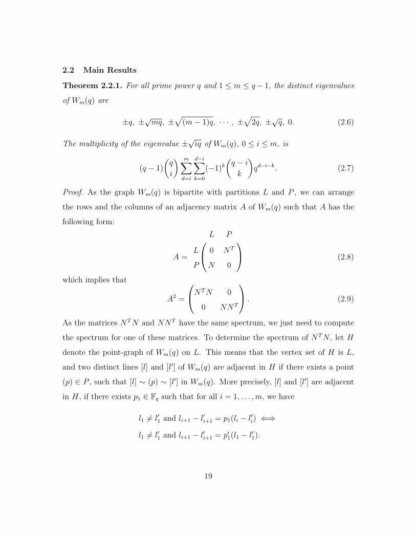
3.2 The Triangular graph T (5). . . . . . . . . . . . . . . . . . . . . . 27

3.3 The minimum disconnecting set in a primitive strongly regulargraph. . . . . . . . . . . . . . . . . . . . . . . . . . . . . . . . . . 30

4.1 The disconnecting set in Brouwer’s conjecture. . . . . . . . . . . . 34

4.2 The Triangular graph T (6) with its disconnecting set colored byred. . . . . . . . . . . . . . . . . . . . . . . . . . . . . . . . . . . 35

5.1 The only two strongly regular graphs which are not 2-extendable.The non-extendable matchings of size 2 are highlighted . . . . . . 58

5.2 The three strongly regular graphs with k ≥ 6 which are not3-extendable. The non-extendable matchings of size 3 arehighlighted. Deleting the highlighted matching in each graph willisolate a vertex, thus the remaining graph does not have a perfectmatching. . . . . . . . . . . . . . . . . . . . . . . . . . . . . . . . 71

6.1 Distance-distribution diagram . . . . . . . . . . . . . . . . . . . . 91

6.2 Petersen graph with distance partition . . . . . . . . . . . . . . . 92

x

ABSTRACT

The algebraic methods have been very successful in understanding the struc-

tural properties of graphs. In general, we can use the eigenvalues of the adjacency

matrix of a graph to study various properties of graphs. In this thesis, we obtain the

whole spectrum of a family of graphs called Wenger graphs Wm(q). We also study

the a conjecture of Brouwer, concerning the second connectivity of strongly regu-

lar graphs. Finally, we compute the extendability of matchings for many strongly

regular graphs and many distance-regular graphs.

xi

Chapter 1

INTRODUCTION

1.1 Introduction

In mathematics and computer science, graph theory studies the combinatorial

objects called graphs. They are mathematical structures used to model pairwise

relations between objects. A graph in this context is made up of vertices or nodes

and lines called edges that connect them.

Figure 1.1: An example of graph with 6 vertices and 7 edges.

Using algebraic properties of matrices associated to graphs, we can study the

combinatorial properties of graphs. For example, spectral graph theory makes use of

Laplacian matrices and adjacency matrices of graphs. Many important combinatorial

1

properties of graphs could be revealed by examining of the eigenvalues and eigen-

vectors of those matrices. Such properties include connectivity and edge expansion,

which will be discussed later in this chapter.

In this thesis, we will focus on adjacency matrices. Adjacency matrices are

useful tools in graph theory, both practically and theoretically. The Perron-Frobenius

eigenvector of the adjacency matrix of the web graph gives rise to a ranking of all the

vertices. It is this very vector that makes the founders of Google billionaires. The

second largest eigenvalue of a graph gives information about diameter and expansion.

The construction of sparse graphs with large spectral gap (the difference between the

first and the second eigenvalues) is a central task in graph theory. Fix an integer

k, the k-regular graphs with “largest” spectral gap are Ramanujan graphs. The

construction of such graphs helps to build a sparse and highly connected network in

internet, thus providing high speed communication and lowering the cost of building

the network. Using Ramanujan graphs, many companies (e.g. Akamai Technologies)

have constructed Content Distribution Network, one of the most important types of

networks nowadays. Such network allows companies (e.g. Microsoft) to provide

higher download speed for their software. Theoretically, eigenvalues also help us

to understand the structure of graphs. The smallest eigenvalue gives information

about independence number and chromatic number. Eigenvalues interlacing gives

information about substructures of graphs. The fact that eigenvalue multiplicities

must be integral provides strong restrictions. All the eigenvalues together provide a

useful graph invariant.

Before we discuss the relations between eigenvalues and graph properties,

we first provide some background in graph theory. For undefined notations, see

Bollobas [11]. In the most common sense of the term, a simple graph is an ordered

pair Γ = (V,E) comprising a set V of vertices or nodes together with a set E of edges

2

or lines, which are 2-element subsets of V (i.e., an edge is related with two vertices,

and the relation is represented as an unordered pair of the vertices with respect to

the particular edge). In this thesis, we only consider simple graphs. Assume that

V = {v1, . . . , vn} and E = {e1, . . . , em}. We say vi and vj are adjacent if and only if

e = {vi, vj} ∈ E. In this case, we write vi ∼ vj. For simplicity, an edge {vi, vj} ∈ E

will be denoted vivj, where vi and vj are the endpoints of the edge. If a vertex v is

an endpoint of an edge e, we say v is incident with e. I included several important

examples of graphs here:

1. The complete graph Kn is the graph on n vertices such that every two vertices

are joined by an edge.

2. The complete bipartite graph Km,n is the graph with vertex set is the union of

2 partite sets V = X ∪ Y , where X ∩ Y = ∅, |X| = m and |Y | = n. Two

vertices u and v are adjacent iff they are in different partite sets.

3. The complete multipartite graph Km×n is the graph with vertex set is the union

of m partite sets V = X1 ∪ . . .∪Xm, where |Xi| = n. Two vertices u and v are

adjacent iff they are in different partite sets.

4. The path Pn is the graph with vertex set [n] := {1, . . . , n} such that i ∼ j if

and only if |i− j| = 1.

5. The cycle Cn is the graph obtained by adding one edge {1, n} to Pn.

6. The line graph L(Γ) of Γ is the graph with the edge set of Γ as vertex set, where

two vertices are adjacent if the corresponding edges of Γ have an endpoint in

common.

3

Here are some general notations which will be use in this thesis. The degree

of a vertex v is the number of edges incident with v. A graph Γ is called regular of

degree (or valency) k, when every vertex has degree k. The neighborhood of a vertex

v, denoted N(v), is the set of vertices that are adjacent to v. A subgraph H of a

graph Γ is a graph with V (H) ⊆ V (Γ) and E(H) ⊆ E(Γ). A graph H is an induced

subgraph of Γ if E(H) = {uv ∈ E(Γ) | u, v ∈ V (H)}. If H is an induced subgraph

of Γ with vertex set S = V (H), the subgraph induced by S is denoted Γ[S]. The

complement of a graph Γ, denoted Γ, is the graph with V (Γ) = V (Γ) and uv ∈ E(Γ)

if and only if uv 6∈ E(Γ). A clique in a graph Γ is a set that induces a complete graph.

An independent set, or coclique, in a graph is a set that induces an empty graph,

the complement of a complete graph. The cardinality of the largest independent set

of a graph Γ is denoted α(Γ). A walk of length l between two vertices u and v, is

a sequence of vertices u = u0, u1, . . . , ul = v, such that for 0 ≤ i ≤ k − 1, ui is

adjacent to ui+1. If all these vertices are distinct, the walk is a path. If there exists

a path between any two vertices, the graph is connected. Otherwise, the graph is

disconnected. A component of Γ is a maximal connected subgraph. For a connected

graph Γ and any two vertices u, v ∈ V (Γ), the distance d(u, v) between u and v is

the minimum length of any path connecting them. The diameter D is defined to

be maxu,v∈V (Γ) d(u, v). Note that if Γ is disconnected, we defined the diameter to be

infinity.

I will need the following important properties of graphs:

1. A graph Γ is called k-connected if deleting any k−1 vertices does not disconnect

the graph. The connectivity of a graph is defined to be the largest k, such that

the graph is k-connected.

2. Similarly, a graph Γ is called k-edge-connected if deleting any k− 1 edges does

4

not disconnect the graph. The edge-connectivity of a graph is defined to be

the largest k, such that the graph is k-edge-connected.

3. A graph Γ is called bipartite when its vertex set can be partitioned into two

disjoint parts X, Y such that both X and Y are independent sets.

1.2 Adjacency Matrices

Let Γ be a finite simple graph. The adjacency matrix of Γ is the 0-1 matrix

A indexed by the vertex set V (Γ) of Γ, where Axy = 1 when there is an edge from x

to y in Γ and Axy = 0 otherwise.

Suppose Γ is a simple graph with n vertices. Since A is real and symmetric,

all its eigenvalues are real. The spectrum of Γ is defined as the multiset of the

eigenvalues of its adjacency matrix. We write the eigenvalues in decreasing order,

that is θ1 ≥ θ2 ≥ · · · ≥ θn.

There are a lot of things we can say about a graph by looking at its spectrum.

We will present some useful facts which will be used in the later sections.

If Γ is regular of degree k, then its adjacency matrix A has row sums k. We

can write it in matrix form, A~1 = k~1, where ~1 is a column vector with all entries

equal to 1. Actually, k is the largest eigenvalue of Γ, and the multiplicity of k equals

the number of components of Γ. So, k ≥ θ2 ≥ · · · ≥ θn.(See [19, Chapter 3])

If Γ is bipartite, then its adjacency matrix is of the form A =

0 B

BT 0

. It

follows that the spectrum of a bipartite graph is symmetric with respect to 0: if

uv

is an eigenvector with eigenvalue θ, then

u

−v

is an eigenvector with eigenvalue −θ.

The converse is also true. Actually, we have the following theorem.

5

Theorem 1.2.1. [19, Proposition 3.4.1]

(i) A graph Γ is bipartite if and only if for each eigenvalue θ of Γ, also −θ is an

eigenvalue, with the same multiplicity.

(ii) If Γ is connected with largest eigenvalue θ1, then Γ is bipartite if and only if

−θ1 is an eigenvalue of Γ.

Another interesting result is that we can give an upper bound for the diameter

in terms of the number of distinct eigenvalues:

Theorem 1.2.2. [19, Proposition 1.3.3] Let Γ be a connected graph with l distinct

eigenvalues, then the diameter of Γ is at most l − 1.

1.3 Interlacing

A powerful tool used in spectral graph theory is eigenvalue interlacing (for

more details, see [58]). Consider two sequences of real numbers: θ1 ≥ · · · ≥ θn, and

η1 ≥ · · · ≥ ηm with m < n. The second sequence is said to interlace the first one if

for i = 1, . . . ,m,

θi ≥ ηi ≥ θn−m+i.

The interlacing is tight if there exists an integer k, 0 ≤ k ≤ m, such that

θi = ηi for 1 ≤ i ≤ k and θn−m+i = ηi for k + 1 ≤ i ≤ m

Theorem 1.3.1 (Haemers [58]). Let S be a real n ×m matrix such that STS = I.

Let A be a real symmetric matrix of order n with eigenvalues θ1 ≥ . . . ≥ θn. Define

B = STAS and let B have eigenvalues η1 ≥ . . . ≥ ηm and respective eigenvectors

v1, . . . , vm.

(i) The eigenvalues of B interlace those of A.

6

(ii) If ηi = θi or ηi = θn−m+i for some i ∈ [1,m], then B has a ηi-eigenvector v

such that Sv is a ηi-eigenvector of A.

(iii) If for some integer l, ηi = θi, for i = 1, . . . , l (or ηi = θn−m+i for i = l, . . . ,m),

then Svi is a ηi-eigenvector of A for i = 1, . . . , l (respectively i = l, . . . ,m).

(iv) If the interlacing is tight, then SB = AS.

If we take S = [I, 0]T , then B is just a principal submatrix of A and we have

the following consequence.

Theorem 1.3.2 (Cauchy Interlacing ). [63, p.185] If B is a principal submatrix of

a symmetric matrix A, then the eigenvalues of B interlace the eigenvalues of A.

This result implies that if H is an induced subgraph of a graph Γ, then the

eigenvalues of H interlace the eigenvalues of Γ. In order to get more eigenvalue

interlacing results, we need to introduce another important matrix.

Consider a partition V (Γ) = V1 ∪ . . . ∪ Vs of the vertex set of Γ into s non-

empty subsets. For 1 ≤ i, j ≤ s, let bi,j denote the average number of neighbors in Vj

of the vertices in Vi. The quotient matrix of this partition is the s× s matrix whose

(i, j)-th entry equals bi,j. The partition is called equitable if for each 1 ≤ i, j ≤ s, any

vertex v ∈ Vi has exactly bi,j neighbors in Vj. Another consequence of Theorem 1.3.1

is that the eigenvalues of a quotient matrix interlace the eigenvalues of the adjacency

matrix of a graph.

Theorem 1.3.3. For a graph Γ, let B be the quotient matrix of a partition of V (Γ).

Then the eigenvalues of B interlace those of A. Furthermore, if the interlacing is

tight, then the partition is equitable.

A consequence of Theorem 1.3.3 is the famous Hoffman Ratio bound. This

bound will be used in Chapters 4 and 5.

7

Theorem 1.3.4 (Hoffman Ratio bound). (See [19, Theorem 3.5.2]) If Γ is a con-

nected, k-regular graph, then

α(Γ) ≤ n−θnk − θn

,

and if an independent set C meets this bound, then every vertex not in C is adjacent

to precisely −θn vertices of C.

Proof. We can partition the vertex set V (Γ) into C and V (Γ)\C. The corresponding

quotient matrix of A is

B =

0 k

kαn−α k − kα

n−α

,where α = α(Γ). The matrix B has eigenvalues η1 = k = θ1 (the row sum) and

η2 = −kα/(n − α) (the matrix trace). By interlacing, θn ≤ η2 = −kα/(n − α).

This gives the required inequality. The second part of the theorem follows from

the fact that when equality happens, the interlacing is tight. Thus, the partition is

equitable.

1.4 Spectral Gap and Edge Expansion

Assume that Γ is k-regular. One of the most well-studied eigenvalue of Γ is

the second eigenvalue θ2. (See the survey by Hoory, Linial and Wigderson [66]) If

the spectral gap k− θ2 is large, then the graph has good connectivity, expansion and

randomness properties. In this section, we discuss the relation between the spectral

gap and edge expansion.

Let A and B be vertex-disjoint subset of V (Γ). Let E(A,B) denote the set

of edges with one endpoint in A and the other one in B, and e(A,B) be the size of

E(A,B). In particular, E(A,Ac) is a cut-set of Γ, where Ac := V (Γ) \ A.

8

Theorem 1.4.1 ([18, 85]). Let Γ be a connected k-regular graph with v vertices. If

A is a vertex subset of size a, then

e(A,Ac) ≥ (k − θ2)a(v − a)

v.

The edge expansion constant h(Γ) (a.k.a. isoperimetric constant or Cheeger

number) of a graph Γ is defined as the minimum of e(S,V \S)|S| , where the minimum is

taken over all non-empty S with |S| ≤ |V (Γ)|/2.

Theorem 1.4.2 (Alon and Milman [3]). Let Γ be a regular graph of degree k, not

Kn with n ≤ 3. Then1

2(k − θ2) ≤ h(Γ) ≤

√k2 − θ2

2.

1.5 Groups, Characters and Finite Fields

Abstract algebra plays an important role in graph theory because many impor-

tant families of graphs can be constructed using well-understood algebraic structures.

On the other hand, the spectrum of many graphs can be computed by character sums.

In this section, I will review some basic facts of abstract algebra. All these results

can be found in many algebra books, for example, see Isaacs [68] or Dummit and

Foote [47].

A group G is a set together with a binary operation ∗ (say) satisfying the

following axioms:

1. a, b ∈ G implies a ∗ b ∈ G (closure);

2. a, b, c ∈ G implies (a ∗ b) ∗ c = a ∗ (b ∗ c) (associativity);

3. there is an element called the identity e ∈ G such that a ∗ e = e ∗ a = a for all

a ∈ G (identity element);

9

4. for any a ∈ G, there is a b ∈ G so that a ∗ b = b ∗ a = e (inverses); we write

a−1 to denote the inverse of a.

If in addition to this, a ∗ b = b ∗ a for all a, b ∈ G, we say that G is abelian or

commutative. When G is finite, we call the size of G the order of G. To indicate a∗ b

we sometimes drop the ∗ and simply write ab with no cause for confusion. In this

case, we assume that the group is multiplicative and we use the symbol 1 to denote

the identity element. If we want to emphasize that the groups we are dealing with

are additive, we will write the group operation as the symbol +. And the symbol 0

will be the identity element.

Here are some examples of groups which will be used later:

1. Z under addition.

2. C∗, non-zero complex numbers under multiplication.

3. Z/nZ under addition consists of residue classes modulo n. This is a finite

abelian group of order n.

4. (Z/pZ)∗ is the set of coprime residue classes mod p, with p prime. This is a

finite abelian group of order p− 1.

Theorem 1.5.1. If G is a finite abelian group of order n, then gn = 1 for any

element g ∈ G.

A character χ of an abelian group G is a map

χ : G→ C∗,

such that χ(ab) = χ(a)χ(b). It is an example of a homomorphism. The character

that sends every element to the element 1 is called the trivial character. It is easy

to check the following facts about characters,

10

1. χ(1) = 1;

2. χ(a−1) = χ(a)−1;

3. If G is a finite group of order n, then χ(g) must be an n-th root of unity.

If G is a finite abelian group of order n, then there are exactly n distinct

characters. In this case, the set of characters forms a group under multiplication of

characters, where the product of two characters χ and ψ is defined in the following

way:

(χψ)(a) := χ(a)ψ(a),

where χ and ψ are characters from G to C∗. We call this the character group of G

and denote it by G. The identity element of G is the trivial character. The character

inverse to χ is χ−1 defined by

χ−1(a) = χ(a)−1.

A field F is a set together with two binary operations + and ◦ satisfying the

following three conditions:

1. the algebraic structure (F,+) is an abelian group.

2. the algebraic structure (F ∗, ◦) is an abelian group, where F ∗ = F \ {0} and 0

is the identity element in (F,+).

3. the operation ◦ distributes over +, i.e. for all x, y, z ∈ F , we have x ◦ (y+ z) =

(x ◦ y) + (x ◦ z).

Well-known examples are the rational numbers Q, the real numbers R and

the complex numbers C under addition and multiplication.

11

A finite field is a field with a finite number of elements. We have already seen

that Z/pZ is a finite field when p is a prime number. Actually, we have the following

two theorems for finite fields:

Theorem 1.5.2. The number of elements in a finite field is a power of a prime.

Theorem 1.5.3. Let n ≥ 1 be an integer and p be a prime. Then there exists a

unique finite field with pn elements.

From now on, we will use Fq to denote the finite field with q elements, where

q is a prime power. As Fq has two operations, each operation will give rise to a

character. We will just mention the additive characters since will need to use them

in Chapter 2.

Let ω = e2πi/p be a complex p-th root of unity, where i is the imaginary

number. For x ∈ Fq, the trace of x is defined as tr(x) =∑e−1

k=0 xpk . Since (Fq,+)

has q characters, we can index each character by an element of Fq. Let ψj be one of

those q characters of (Fq,+), where j ∈ Fq. When applying ψj to an element a ∈ Fq,

we have ψj(a) = ωtr(ja).

1.6 Cayley Graphs

There is a simple procedure for constructing k-regular graphs. It proceeds as

follows. Let G be an abelian group and S a k-element subset of G. We require that

S is symmetric in the sense that s ∈ S implies s−1 ∈ S. The Cayley graph on G with

generating set S is the graph Γ with vertex set G and edge set E = {(x, y) | x−1y ∈

S}. We denote this graph by Cay(G,S). Note that Cay(G,S) is regular with degree

|S|. One immediate example is the cycle Cn, which is Cay(Z/nZ, {−1, 1}), where

the group is under addition.

12

Suppose that χ is a character of G. It is easy to check that (χ(g))g∈G is an

eigenvector of the adjacency matrix of Cay(G,S). The eigenvalues of the Cayley

graph of an abelian group are easily determined as follows.

Theorem 1.6.1. Let G be a finite abelian group and S a symmetric subset of G of

size k. Then the eigenvalues of the adjacency matrix of Cay(G,S) are given by

θχ =∑s∈S

χ(s),

where χ ranges over all the characters of G.

There is a generalization of the above theorem to non-abelian groups. This

is essentially contained in Babai [5] and Diaconis and Shahshahani [46]. To state

the theorem, we need to use the concept of an irreducible character. For details of

irreducible characters, see Sagan [94].

Theorem 1.6.2. Let G be a finite group and S a symmetric subset which is stable

under conjugation. Then the eigenvalues of the adjacency matrix of Cay(G,S) are

given by

θχ =1

χ(1)

∑s∈S

χ(s)

where χ ranges over all irreducible characters of G. Moreover, the multiplicity of θχ

is χ(1)2.

13

Chapter 2

SPECTRUM OF WENGER GRAPHS

In this chapter, we will compute the whole spectrum of a family of graph

Wm(q) which are defined by a family of equations over finite fields. It turns out

that for certain parameter sets, those graphs have large spectral gap, and thus have

large edge expansion. Most of the results of this chapter have appeared in Cioaba,

Lazebnik and Li [35].

2.1 Introduction

Let q = pe, where p is a prime and e ≥ 1 is an integer. For m ≥ 1, let P

and L be two copies of the (m+ 1)-dimensional vector spaces over the finite field Fq.

We call the elements of P points and the elements of L lines. If a ∈ Fm+1q , then we

write (a) ∈ P and [a] ∈ L. Consider the bipartite graph Wm(q) with partite sets P

and L defined as follows: a point (p) = (p1, p2, . . . , pm+1) ∈ P is adjacent to a line

[l] = [l1, l2, . . . , lm+1] ∈ L if and only if the following m equalities hold:

l2 + p2 = l1p1 (2.1)

l3 + p3 = l2p1 (2.2)

... (2.3)

lm+1 + pm+1 = lmp1. (2.4)

The graph Wm(q) has 2qm+1 vertices, is q-regular and has qm+2 edges.

14

In [105], Wenger introduced a family of p-regular bipartite graphs Hk(p) as

follows. For every k ≥ 2, and every prime p, the partite sets of Hk(p) are two

copies of integer sequences {0, 1, . . . , p− 1}k, with vertices a = (a0, a1, . . . , ak−1) and

b = (b0, b1, . . . , bk−1) forming an edge if

bj ≡ aj + aj+1bk−1 (mod p) for all j = 0, . . . , k − 2.

The introduction and study of these graphs were motivated by an extremal graph

theory problem of determining the largest number of edges in a graph of order n

containing no cycle of length 2k. This parameter also known as the Turan number

of the cycle C2k, is denoted by ex(n,C2k). Bondy and Simonovits [12] showed that

ex(n,C2k) = O(n1+1/k), n → ∞. Lower bounds of magnitude n1+1/k were known

(and still are) for k = 2, 3, 5 only, and the graphs Hk(p), k = 2, 3, 5, provided new

and simpler examples of such magnitude extremal graphs. For many results on

ex(n,C2k), see Verstraete [101], Pikhurko [93] and references therein.

In [71], Lazebnik and Ustimenko, using a construction based on a certain Lie

algebra, arrived at a family of bipartite graphs H ′n(q), n ≥ 3, q is a prime power,

whose partite sets were two copies of Fn−1q , with vertices (p) = (p2, p3, . . . , pn) and

[l] = [l1, l3, . . . , ln] forming an edge if

lk − pk = l1pk−1 for all k = 3, . . . , n.

It is easy to see that for all k ≥ 2 and prime p, graphs Hk(p) and H ′k+1(p) are

isomorphic, and the map

φ : (a0, a1, . . . , ak−1) 7→ (ak−1, ak−2, . . . , a0),

(b0, b1, . . . , bk−1) 7→ [bk−1, bk−2, . . . , b0],

15

provides an isomorphism from Hk(p) to H ′k+1(p). Hence, graphs H ′n(q) can be viewed

as generalizations of graphs Hk(p). It is also easy to show that graphs H ′m+2(q) and

Wm(q) are isomorphic: the function

ψ : (p2, p3, . . . , pm+2) 7→ [p2, p3, . . . , pm+2],

[l1, l3, . . . , lm+2] 7→ (−l1,−l3, . . . ,−lm+1),

mapping points to lines and lines to points, is an isomorphism of H ′m+2(q) to Wm(q).

Combining this isomorphism with the results in [71], we obtain that the graph W1(q)

is isomorphic to an induced subgraph of the point-line incidence graph of the pro-

jective plane PG(2, q), the graph W2(q) is isomorphic to an induced subgraph of

the point-line incidence graph of the generalized quadrangle Q(4, q), and W3(q) is a

homomorphic image of an induced subgraph of the point-line incidence graph of the

generalized hexagon H(q).

We call the graphs Wm(q) Wenger graphs. The representation of Wenger

graphs as Wm(q) graphs first appeared in Lazebnik and Viglione [73]. These authors

suggested another useful representation of these graphs, where the right-hand sides

of equations are represented as monomials of p1 and l1 only, see [102]. For this,

define a bipartite graph W ′m(q) with the same partite sets as Wm(q), where (p) =

(p1, p2, . . . , pm+1) and [l] = [l1, l2, . . . , lm+1] are adjacent if

lk + pk = l1pk−11 for all k = 2, . . . ,m+ 1. (2.5)

The map

ω : (p) 7→ (p1, p2, p′3, . . . , p

′m+1), where p′k = pk +

k−1∑i=2

pipk−i1 , k = 3, . . . ,m+ 1,

[l] 7→ [l1, l2, . . . , lm+1],

16

defines an isomorphism from Wm(q) and W ′m(q).

It was shown in [71] that the automorphism group of Wm(q) acts transitively

on each of P and L, and on the set of edges of Wm(q). In other words, the graphs

Wm(q) are point-, line-, and edge-transitive. A more detailed study, see [73], also

showed that W1(q) is vertex-transitive for all q, and that W2(q) is vertex-transitive

for even q. For all m ≥ 3 and q ≥ 3, and for m = 2 and all odd q, the graphs

Wm(q) are not vertex-transitive. Another result of [73] is that Wm(q) is connected

when 1 ≤ m ≤ q − 1, and disconnected when m ≥ q, in which case it has qm−q+1

components, each isomorphic to Wq−1(q). In [103], Viglione proved that when 1 ≤

m ≤ q − 1, the diameter of Wm(q) is 2m + 2. Note that the statement about the

number of components of Wm(q) becomes apparent from the representation (2.5).

Indeed, as l1pi1 = l1p

i+q−11 , all points and lines in a component have the property that

their coordinates i and j, where i ≡ j mod (q − 1), are equal. Hence, points (p),

having p1 = . . . = pq = 0, and at least one distinct coordinate pi, q + 1 ≤ i ≤ m+ 1,

belong to different components. This shows that the number of components is at

least qm−q+1. As Wq−1(q) is connected and Wm(q) is edge-transitive, all components

are isomorphic to Wq−1(q). Hence, there are exactly qm−q+1 of them. A result of

Watkins [104], and the edge-transitivity of Wm(q) imply that the vertex connectivity

(and consequently the edge connectivity) of Wm(q) equals the degree of regularity q,

for any 1 ≤ m ≤ q − 1.

Shao, He and Shan [96] proved that in Wm(q), q = pe, p prime, for m ≥ 2,

for any integer l 6= 5, 4 ≤ l ≤ 2p and any vertex v, there is a cycle of length 2l

passing through the vertex v. Note that the edge-transitivity of Wm(q) implies the

existence of a 2l cycle through any edge, a stronger statement. Li and Lih [74] used

the Wenger graphs to determine the asymptotic behavior of the Ramsey number

rn(C2k) = Θ(nk/(k−1)) when k ∈ {2, 3, 5} and n → ∞; the Ramsey number rn(G)

17

equals the minimum integer N such that in any edge-coloring of the complete graph

KN with n colors, there is a monochromatic G. Representation (2.5) points to a

relation of Wenger graphs with the moment curve t 7→ (1, t, t2, t3, ..., tm), and, hence,

with Vandermonde’s determinant, which was explicitly used in [105]. This is also

in the background of some geometric constructions by Mellinger and Mubayi [84] of

magnitude extremal graphs without short even cycles.

In Section 2.2, we determine the spectrum of the graphs Wm(q). Futorny

and Ustimenko [52] considered applications of Wenger graphs in cryptography and

coding theory, as well as some generalizations. They also conjectured that the second

largest eigenvalue θ2 of the adjacency matrix of Wenger graphs Wm(q) is bounded

from above by 2√q. The results of this chapter confirm the conjecture for m = 1

and 2, or m = 3 and q ≥ 4, and refute it in other cases. We wish to point out

that for m = 1 and 2, or m = 3 and q ≥ 4, the upper bound 2√q also follows

from the known values of θ2 for the point-line (q + 1)-regular incidence graphs of

the generalized polygons PG(2, q), Q(4, q) and H(q) and eigenvalue interlacing (see

Brouwer, Cohen and Neumaier [17]). In [75], Li, Lu and Wang showed that the

graphs Wm(q), m = 1, 2, are Ramanujan, by computing the eigenvalues of another

family of graphs described by systems of linear equations in [72], D(k, q), for k = 2, 3.

Their result follows from the fact that W1(q) ' D(2, q), and W2(q) ' D(3, q). For

more on Ramanujan graphs, see Lubotzky, Phillips and Sarnak [82], or Murty [87].

Our results also imply that for fixed m and large q, the Wenger graph Wm(q) are

expanders. For more details on expanders and their applications, see Hoory, Linial

and Wigderson [66], and references therein.

18

2.2 Main Results

Theorem 2.2.1. For all prime power q and 1 ≤ m ≤ q− 1, the distinct eigenvalues

of Wm(q) are

±q, ±√mq, ±√

(m− 1)q, · · · , ±√

2q, ±√q, 0. (2.6)

The multiplicity of the eigenvalue ±√iq of Wm(q), 0 ≤ i ≤ m, is

(q − 1)

(q

i

) m∑d=i

d−i∑k=0

(−1)k(q − ik

)qd−i−k. (2.7)

Proof. As the graph Wm(q) is bipartite with partitions L and P , we can arrange

the rows and the columns of an adjacency matrix A of Wm(q) such that A has the

following form:

A =

L P

L 0 NT

P N 0

(2.8)

which implies that

A2 =

NTN 0

0 NNT

. (2.9)

As the matrices NTN and NNT have the same spectrum, we just need to compute

the spectrum for one of these matrices. To determine the spectrum of NTN , let H

denote the point-graph of Wm(q) on L. This means that the vertex set of H is L,

and two distinct lines [l] and [l′] of Wm(q) are adjacent in H if there exists a point

(p) ∈ P , such that [l] ∼ (p) ∼ [l′] in Wm(q). More precisely, [l] and [l′] are adjacent

in H, if there exists p1 ∈ Fq such that for all i = 1, . . . ,m, we have

l1 6= l′1 and li+1 − l′i+1 = p1(li − l′i) ⇐⇒

l1 6= l′1 and li+1 − l′i+1 = pi1(l1 − l′1).

19

This implies that H is actually the Cayley graph of the additive group of the vector

space Fm+1q with a generating set

S = {(t, tu, . . . , tum) | t ∈ F∗q, u ∈ Fq}. (2.10)

Let ω be a complex p-th root of unity. Recall that for x ∈ Fq, the trace of x

is defined as tr(x) =∑e−1

k=0 xpk . The eigenvalues of H are indexed after the (m+ 1)-

tuples (w1, . . . , wm+1) ∈ Fm+1q . By Theorem 1.6.1, they can be represented in the

following form:

θ(w1,...,wm+1) =∑

(t,tu,...,tum)∈S

ωtr(tw1) · ωtr(tuw2) · · · · · ωtr(tumwm+1)

=∑

t∈F∗q , u∈Fq

ωtr(tw1+tuw2+···+tumwm+1)

=∑

t∈F∗q , u∈Fq

ωtr(t(f(u))) (where f(u) := w1 + w2u+ · · ·+ wm+1um)

=∑

t∈F∗q , f(u)=0

ωtr(t(f(u))) +∑

t∈F∗q , f(u)6=0

ωtr(t(f(u))).

Note that θ(w1,...,wm+1) here can be considered as a Jacobi sum. For more details

regarding Jacobi sums, see Ireland and Rosen [67, Chapter 8]. As∑

t∈F∗qωtr(tx) = q−1

for x = 0, and∑

t∈F∗qωtr(tx) = −1 for every x ∈ F∗q, we obtain that

θ(w1,...,wm+1) = |{u ∈ Fq | f(u) = 0}|(q − 1)− |{u ∈ Fq | f(u) 6= 0}|. (2.11)

Let B be the adjacency matrix of H. Then NTN = B+ qI. This implies that

the eigenvalues of Wm(q) can be written in the form

±√θ(w1,...,wm+1) + q,

20

where (w1, . . . , wm+1) ∈ Fm+1q . Let f(X) = w1 +w2X + · · ·+wm+1X

m ∈ Fq[X]. We

consider two cases.

1. f = 0. In this case, |{u ∈ Fq | f(u) = 0}| = q, and θ(w1,...,wm+1) = q(q − 1).

Thus, Wm(q) has ±q as its eigenvalues.

2. f 6= 0. In this case, let i = |{u ∈ Fq | f(u) = 0}| ≤ m as 1 ≤ m ≤ q − 1.

This shows that θ(w1,...,wm+1) = i(q − 1) − (q − i) = iq − q and implies that

±√θ(w1,...,wm+1) + q = ±

√iq are eigenvalues of Wm(q). Note that for any 0 ≤

i ≤ m, there exists a polynomial f over Fq of degree at most m ≤ q− 1, which

has exactly i distinct roots in Fq. For such f , |{u ∈ Fq | f(u) = 0}| = i,

and, hence, there exists (w1, . . . , wm+1) ∈ Fm+1q , such that θ(w1,...,wm+1) = iq−q.

Thus, Wm(q) has ±√iq as its eigenvalues, for any 0 ≤ i ≤ m, and the first

statement of the theorem is proven.

The arguments above imply that the multiplicity of the eigenvalue ±√iq of

Wm(q) equals the number of polynomials of degree at most m (not necessarily monic)

having exactly i distinct roots in Fq. To calculate these multiplicities, we need

the following lemma. Particular cases of the lemma were considered in Zsigmondy

[108], and in Cohen [37]. The complete result appears in A. Knopfmacher and

J. Knopfmacher [70].

Lemma 2.2.2 ([70]). Let q be a prime power, and let d and i be integers such that

0 ≤ i ≤ d ≤ q − 1. Then the number b(q, d, i) of monic polynomials in Fq[X] of

degree d, having exactly i distinct roots in Fq is given by

b(q, d, i) =

(q

i

) d−i∑k=0

(−1)k(q − ik

)qd−i−k. (2.12)

21

By Lemma 2.2.2, the number of polynomials of degree at most m in Fq[X]

(not necessarily monic) having exactly i distinct roots in Fq is

m∑d=i

(q − 1) b(q, d, i) = (q − 1)

(q

i

) m∑d=i

d−i∑k=0

(−1)k(q − ik

)qd−i−k. (2.13)

This concludes the proof the theorem.

The previous result shows that Wm(q) is connected and has 2m + 3 distinct

eigenvalues, for any 1 ≤ m ≤ q − 1. By Theorem 1.2.2, the diameter of a graph is

strictly less than the number of distinct eigenvalues. This implies that the diameter

of Wenger graph is less or equal to 2m + 2. This is actually the exact value of the

diameter of the Wenger graph as shown by Viglione [103].

Since the sum of multiplicities of all eigenvalues of the graph Wm(q) is equal

to its order, and remembering that the multiplicity of ±q is one when 1 ≤ m ≤ q−1,

we have a combinatorial proof of the following identity.

Corollary 2.2.3. For every prime power q, and every m, 1 ≤ m ≤ q − 1,

m∑i=0

(q

i

) m∑d=i

d−i∑k=0

(−1)k(q − ik

)qd−i−k =

qm+1 − 1

q − 1. (2.14)

The identity (2.14) seem to hold for all integers q ≥ 3, so a direct proof is

desirable. Other identities can be obtained by taking the higher moments of the

eigenvalues of Wm(q).

As we discussed in the introduction, for m ≥ q, the graph Wm(q) has qm−q+1

components, each isomorphic to Wq−1(q). This, together with Theorem 2.2.1, imme-

diately implies the following.

Proposition 2.2.4. For m ≥ q, the distinct eigenvalues of Wm(q) are

±q, ±√

(q − 1)q, ±√

(q − 2)q, · · · , ±√

2q, ±√q, 0,

22

and the multiplicity of the eigenvalue ±√iq, 0 ≤ i ≤ q − 1, is

(q − 1)qm+1−q(q

i

) q∑d=i

d−i∑k=0

(−1)k(q − ik

)qd−i−k.

2.3 Remarks

In 1995, Lazebnik and Ustimenko [72] constructed an infinite family of graphs

D(k, q) of high density and without any cycle of length strictly less than k+5. Their

construction is as follows:

Let q be a prime power, and let P and L be two copies of the countably

infinite dimensional vector space V over Fq. By D(q) we denote a bipartite graph

with the bi-partition (P,L) and edges defined as follows. We say that vertices (p) ∈

(p1, p2, p3, . . .) ∈ P and [l] ∈ [l1, l2, l3, . . .] ∈ L are adjacent if and only if the following

relations on their coordinates hold:

l2 − p2 = l1p1

l3 − p3 = l2p1

l4i − p4i = l1p4i−2

l4i+1 − p4i+1 = l1p4i−1

l4i+2 − p4i+2 = l4ip1

l4i+3 − p4i+3 = l4i+1p1

for all i = 1, 2, . . .

For each positive integer k ≥ 2, let Pk and Lk be canonical projections of P and

L onto their k initial coordinates. Imposing the first k − 1 adjacency relations on

vectors from Pk and Lk, we obtain a bipartite graph of order 2qk with bi-partition

(Pk, Lk). Denote this graph D(k, q). For odd k, the girth of D(k, q) is at least k+ 5.

23

Note that D(k, q) is defined by more complicated equations. And the point-

graph of D(k, q) on Lk or the line-graph of D(k, q) on Pk is not a Cayley graph.

We can not apply the same method to compute the its spectrum as in the spectrum

of Wenger graph. It will be interesting if one can compute the spectrum of those

graphs.

Motivated by our computation of the spectrum of Wenger graphs, Cao, Lu,

Wan, Wang and Wang [28] used techniques similar to Theorem 2.2.1 and computed

the spectrum of Linearized Wenger graphs Lm(q). The definition of these graphs is

similar to the construction of Wenger graphs. The only difference is equation (2.5).

A point (p) = (p1, p2, . . . , pm+1) ∈ P is adjacent to a line [l] = [l1, l2, . . . , lm+1] ∈ L if

and only if

lk + pk = l1(p1)pk−2

for all k = 2, . . . ,m+ 1. (2.15)

Cao, Lu, Wan, Wang and Wang [28] also determined the diameter and girth of

linearized Wenger graphs. However, they can not find an explicit formula for the

eigenvalue multiplicities of the linearized Wenger graphs when m < e, where q = pe.

24

Chapter 3

STRONGLY REGULAR GRAPHS

In this chapter, I will give some facts about strongly regular graphs which will

be used in the next two chapters, see [19, 56] for more details.

3.1 Introduction

A graph Γ is said to be strongly regular with parameters (v, k, λ, µ) (short-

handed (v, k, λ, µ)-SRG from now on) if Γ is k-regular with v vertices, every adjacent

pair of vertices have λ common neighbors, and every non-adjacent pair of vertices

have µ common neighbors. The study of strongly regular graphs lies at the intersec-

tion of graph theory, algebra and finite geometry [22, 25, 26] and has applications in

coding theory and computer science, among others [27, 97]. Note that if Γ is strongly

regular with parameters (v, k, λ, µ), then Γ is also strongly regular with parameters

(v, v− k− 1, v− 2− 2k+ µ, v− 2k+ λ). It is easy to tell whether a strongly regular

graph is connected by looking at its parameters.

Lemma 3.1.1. Let Γ be a (v, k, λ, µ)-SRG which is not Kv or Kv. The following

are equivalent:

1. Γ is disconnected.

2. λ = k − 1.

3. µ = 0.

25

4. Γ is a disjoint union of m copies of Kk+1, where m = v/(k + 1).

A strongly regular graph is called imprimitive if it, or its complement, is

disconnected, and primitive otherwise. Two examples of strongly regular graph are

the cycle C5 and the Petersen graph. Their parameters are (5, 2, 0, 1) and (10, 3, 0, 1),

respectively. There are many constructions of strongly regular graphs. I will present

three well-known families of strongly regular graphs in this section.

1. Let q = 4t+1 be a prime power. The Paley graph Paley(q) is a (q, q−12, q−5

4, q−1

4)-

SRG. It is the Cayley graph Cay(Fq, (F∗q)2), where Fq is the finite field with

order q and (F∗q)2 is the set of non-zero squares in the field.

2. The Lattice graph Ln is a strongly regular graph with parameters (n2, 2(n −

1), n− 2, 2). It is the line graph of the complete bipartite graph Kn,n.

Figure 3.1: The Lattice graph L3.

3. The Triangular graph T (m) is a strongly regular graph with parameter ((m2

), 2m−

4,m − 2, 4). It is the line graph of the complete graph Km. The vertices

26

of T (m) are the 2-subsets of {1, . . . ,m} and {u, v} ∼ {x, y} if and only if

|{u, v} ∩ {x, y}| = 1.

Figure 3.2: The Triangular graph T (5).

3.2 Eigenvalues of Strongly Regular Graphs

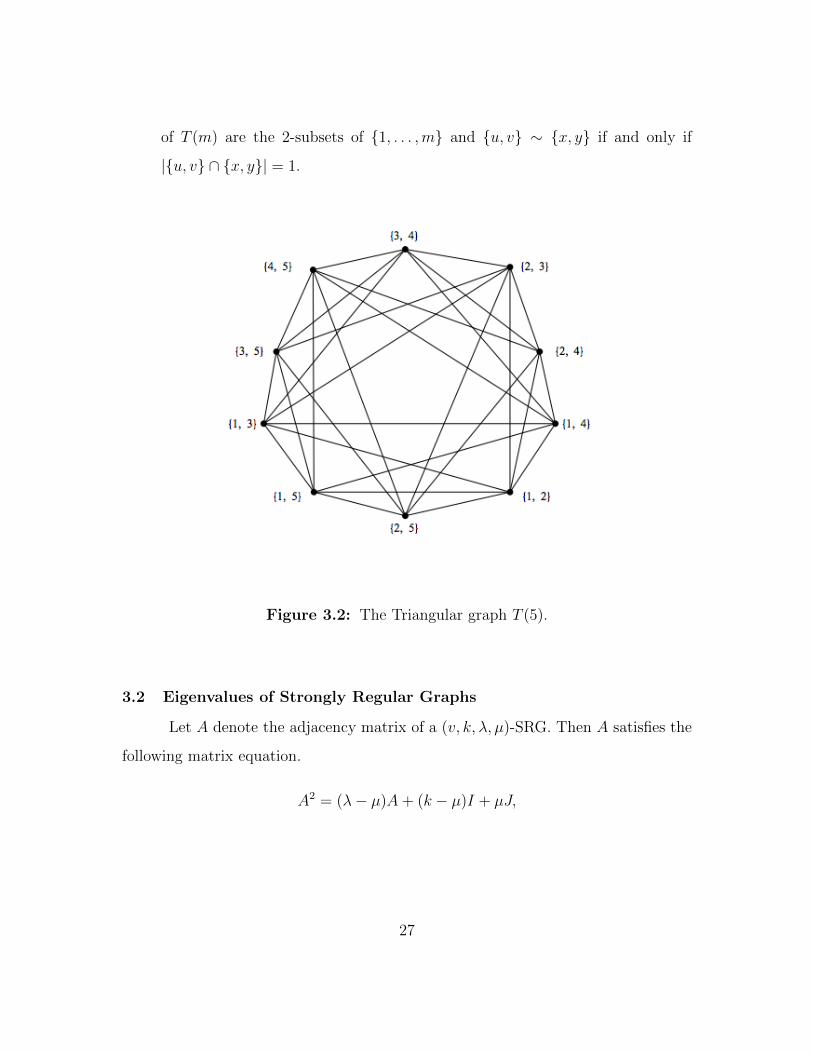
Let A denote the adjacency matrix of a (v, k, λ, µ)-SRG. Then A satisfies the

following matrix equation.

A2 = (λ− µ)A+ (k − µ)I + µJ,

27

where J is the all ones matrix. Consider an eigenvector ~x of A orthogonal to the all

ones vector ~1 (which is an eigenvector of A corresponding to k) with corresponding

eigenvalue γ. Applying ~x to the above equation reduces to

γ2 − (λ− µ)γ − (k − µ) = 0.

Any eigenvalue of A that is not equal to k must be a solution to the above equation,

thus A has exactly three distinct eigenvalues. Let k > θ2 > θv be the distinct

eigenvalues of Γ, then

θ2 =λ− µ+

√(λ− µ)2 + 4(k − µ)

2,

θv =λ− µ−

√(λ− µ)2 + 4(k − µ)

2,

Let m2 and mv denote the multiplicity of the eigenvalues θ2 and θv, respec-

tively. Since k has multiplicity 1 and the trace of A is 0,

m2 +mv = v − 1 and m2θ2 +mvθv = −k.

This yields

m2 =(v − 1)θv + k

θv − θ2

and mv = −(v − 1)θ2 + k

θv − θ2

.

Substituting the values of θ2 and θv,

m2 =1

2

(v − 1− 2k + (v − 1)(λ− µ)√

(λ− µ)2 + 4(k − µ)

)

mv =1

2

(v − 1 +

2k + (v − 1)(λ− µ)√(λ− µ)2 + 4(k − µ)

).

Strongly regular graphs with m2 = mv are called conference graphs. Such

graphs have parameters (v, k, λ, µ) = (4t + 1, 2t, t − 1, t). The Paley graphs belong

to this case, but there are many further examples. It is well-known that a strongly

regular graph is either a conference graph or all its eigenvalues are integer.

28

3.3 Seidel’s Classification of Strongly Regular Graphs

The following is Seidel’s classification (see [95] or [18, Section 9.2]) of the

strongly regular graphs with smallest eigenvalue θv = −2, which will be used in

Chapter 4 and 5.

Theorem 3.3.1. Let Γ be a strongly regular graph with smallest eigenvalue −2.

Then Γ is one of

(i) the complete n-partite graph Kn×2, with parameters (v, k, λ, µ) = (2n, 2n −

2, 2n− 4, 2n− 2), n ≥ 2,

(ii) the lattice graph L(Kn,n), n ≥ 3,

(iii) the Shrikhande graph, with parameters (v, k, λ, µ) = (16, 6, 2, 2),

(iv) the triangular graph T (n) , n ≥ 5,

(v) one of the three Chang graphs, with parameters (v, k, λ, µ) = (28, 12, 6, 4),

(vi) the Petersen graph, with parameters (v, k, λ, µ) = (10, 3, 0, 1),

(vii) the Clebsch graph, with parameters (v, k, λ, µ) = (16, 10, 6, 6),

(viii) the Schlafli graph, with parameters (v, k, λ, µ) = (27, 16, 10, 8).

Strongly regular graphs have high connectivity. In 1985, Brouwer and Mes-

ner (see [23] or [18, Section 9.3]) used eigenvalue interlacing and Theorem 3.3.1 to

compute the vertex-connectivity of any connected strongly regular graph.

Theorem 3.3.2 (Brouwer and Mesner [23]). If Γ is a primitive strongly regular

graph of valency k, then Γ is k-connected. Any disconnecting set of size k must be

the neighborhood of some vertex.

29

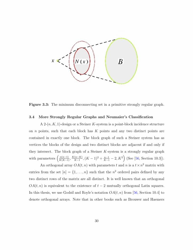
Figure 3.3: The minimum disconnecting set in a primitive strongly regular graph.

3.4 More Strongly Regular Graphs and Neumaier’s Classification

A 2-(n,K, 1)-design or a Steiner K-system is a point-block incidence structure

on n points, such that each block has K points and any two distinct points are

contained in exactly one block. The block graph of such a Steiner system has as

vertices the blocks of the design and two distinct blocks are adjacent if and only if

they intersect. The block graph of a Steiner K-system is a strongly regular graph

with parameters(n(n−1)K(K−1)

, K(n−K)K−1

, (K − 1)2 + n−1K−1− 2, K2

)(See [56, Section 10.3]).

An orthogonal array OA(t, n) with parameters t and n is a t×n2 matrix with

entries from the set [n] = {1, . . . , n} such that the n2 ordered pairs defined by any

two distinct rows of the matrix are all distinct. It is well known that an orthogonal

OA(t, n) is equivalent to the existence of t − 2 mutually orthogonal Latin squares.

In this thesis, we use Godsil and Royle’s notation OA(t, n) from [56, Section 10.4] to

denote orthogonal arrays. Note that in other books such as Brouwer and Haemers

30

[18] the orthogonal array OA(t, n) is denoted by OA(n, t). Given an orthogonal

array OA(t, n), one can define a graph Γ as follows: The vertices of Γ are the n2

columns of the orthogonal array and two distinct columns are adjacent if they have

the same entry in one coordinate position. The graph Γ is an (n2, t(n− 1), n− 2 +

(t − 1)(t − 2), t(t − 1))-SRG ([56, Section 10.4]). Any strongly regular graph with

such parameters is called a Latin square graph (see [18, Section 9.1.12], [56, Section

10.4] or [76, Chapter 30]). When t = 2 and n 6= 4, such a graph must be the line

graph of Kn,n which is also the graph associated with an orthogonal array OA(2, n)

(see [76, Problem 21F]).

In 1979, Neumaier [88] gave a classification strongly regular graphs with small-

est eigenvalue −m, where m ≥ 2 is a fixed integer, by showing the following theorem.

Theorem 3.4.1. Let m ≥ 2 be a fixed integer. Then with finitely many exceptions,

the strongly regular graphs with smallest eigenvalue are of one of the following types:

(a) Complete multipartite graphs with classes of size m,

(b) Block graphs of Steiner m-systems with parameters(n(n− 1)

m(m− 1),m(n−m)

m− 1, (m− 1)2 +

n− 1

m− 1− 2,m2

),

(c) Latin square graphs with parameters

(n2,m(n− 1), n− 2 + (m− 1)(m− 2),m(m− 1)).

Note that this theorem generalized Theorem 3.3.1, but it did not tell us how

many exceptions there are for each m > 2.

31

3.5 Strongly Regular Graphs from Copolar and ∆-spaces

A pair (P,L), where L ⊆ 2P , is called a partial linear space if (i) every l ∈ L

contains at least two points in P , and (ii) for two distinct p, q ∈ P there is at most

one line l ∈ L that contains both. We call the elements of P points and the elements

in L lines. A point p is on the line l if p ∈ l. Also, two distinct points are collinear

if there is a line that contains both points. A partial linear space (P,L) is called a

copolar space (following Hall [59]) or proper delta space (according to Higman; see

Hall [59] and the references therein) if for any point p and line l, p 6∈ l, p is collinear

with none or all but one of the points of l. A more general notion is the notion of a

∆-space. A partial linear space (P,L) is called a ∆-space if for any point p and line

l, p 6∈ l, p is collinear with none, all but one or all the points of l. We say a partial

linear space (P,L) is of order (s, t) if every line contains exactly s + 1 points, and

every point is in exactly t+ 1 lines.

Assume that the point graph Γ of a ∆-space of order (s, t) (i.e. the graph

with vertex point P where two points are adjacent if they are collinear) is strongly

regular with parameters (v, k, λ, µ) with k = s(t + 1). Hall [59] determined all the

strongly regular graphs that appear as the point graph of a copolar space and these

graphs are: the triangular graphs T (m), the symplectic graphs Sp(2r, q) over the

field Fq for any q prime power, the strongly regular graphs constructed from the

hyperbolic quadrics O+(2r, 2) and from the elliptic quadrics O−(2r, 2) over the field

F2 respectively, and the complements of Moore graphs. At the end of this section, I

will briefly describe Sp(2r, q), O+(2r, 2) and O−(2r, 2) as I will need them in Chapter

4. See [31, Section 5,6,7] for more details.

Let q be a prime power and r ≥ 2 be an integer. If x is a non-zero (column)

vector in F2rq , denote by [x] the 1-dimensional vector subspace of F2r

q that is spanned

32

by x and denote by xt the row vector that is the transpose of x. Let M be the 2r×2r

block diagonal matrix whose diagonal blocks are

0 −1

1 0

.

The symplectic graph Sp(2r, q) over Fq has vertex set formed by the 1-

dimensional subspaces [x] of F2rq with [x] ∼ [y] if and only if xtMy 6= 0. The

symplectic graph Sp(2r, q) is a(q2r−1q−1

, q2r−1, q2r−2(q − 1), q2r−2(q − 1))

-SRG. See [31,

Section 5] for a proof.

The hyperbolic quadric graphs O+(2r, 2) is the subgraph of Sp(2r, 2) induced

by V + := {(x1, . . . , x2r)t ∈ F2r

2 : x1x2 + x3x4 + · · · + x2r−1x2r = 1} (the complement

of a hyperbolic quadric in F2r2 ). The vertex x := (x1, . . . , x2r)

t is adjacent to y :=

(y1, . . . , y2r)t if xtMy = 1, where M is the block diagonal matrix defined above.

It is known [56, Chapter 10] that O+(2r, 2) is a (22r−1 − 2r−1, 22r−2 − 2r−1, 22r−3 −

2r−2, 22r−3 − 2r−1)-SRG.

The elliptic quadric graph O−(2r, 2) is the subgraph of Sp(2r, 2) induced by

V − := {x1, . . . , x2r)t ∈ F2r

2 : x21 + x2

2 + x1x2 + x3x4 + · · · + x2r−1x2r = 1} (the

complement of an elliptic quadric in F2r2 ). The vertex x := (x1, . . . , x2r)

t is adjacent to

y := (y1, . . . , y2r)t if xtMy = 1, where M is the block diagonal matrix defined above.

It is known [56, Chapter 10] that O−(2r, 2) is a (22r−1 + 2r−1, 22r−2 + 2r−1, 22r−3 +

2r−2, 22r−3 + 2r−1)-SRG.

33

Chapter 4

DISCONNECTING STRONGLY REGULAR GRAPHS

In this chapter, we will study the minimum size of a subset of vertices of

a connected strongly regular graph whose removal disconnects the graph into non-

singleton components. Most of the results of this chapter have appeared in Cioaba,

Kim and Koolen [31] and Cioaba, Koolen and Li [33].

4.1 Introduction

In 1996, Brouwer [14] conjectured that the minimum size of a disconnecting set

of vertices whose removal disconnects a connected (v, k, λ, µ)-SRG into non-singleton

components equals 2k − λ− 2, which is the size of the neighborhood of an edge.

Figure 4.1: The disconnecting set in Brouwer’s conjecture.

Cioaba, Kim and Koolen [31] showed that strongly regular graphs constructed

from copolar spaces and from the more general spaces called ∆-spaces (See Section

34

3.5) are counterexamples to Brouwer’s conjecture. Using J.I. Hall’s characterization

of finite reduced copolar spaces, they found that the triangular graphs T (m), the

symplectic graphs Sp(2r, q) over the field Fq (for any q prime power), and the strongly

regular graphs constructed from the hyperbolic quadrics O+(2r, 2) and from the

elliptic quadrics O−(2r, 2) over the field F2, respectively, are counterexamples to

Brouwer’s Conjecture. We will just present their result on the triangular graphs

T (m).

Proposition 4.1.1 (Cioaba, Kim and Koolen [31]). For m ≥ 6, the minimum size

of a disconnecting set of vertices whose removal disconnects T (m) into non-singleton

components equals 3m − 9 and the only disconnecting sets of this size are formed

(modulo a permutation of [m]) by the set of vertices adjacent to at least one of the

vertices {1, 2}, {1, 3} or {2, 3}.

Figure 4.2: The Triangular graph T (6) with its disconnecting set colored by red.

35

However, it seems that for many families of strongly regular graphs, Brouwer’s

Conjecture is true. Cioaba, Kim and Koolen proved that Brouwer’s Conjecture is

true for many families of strongly regular graphs including the conference graphs,

the point graphs of generalized quadrangles GQ(q, q), the lattice graphs, the Latin

square graphs, the strongly regular graphs with smallest eigenvalue −2 (except the

triangular graphs) and the primitive strongly regular graphs with at most 30 vertices

except for a few cases. In this chapter, we extend several results from [31] and we show

that Brouwer’s Conjecture is true for any (v, k, λ, µ)-SRG with max(λ, µ) ≤ k/4.

This makes significant progress towards solving an open problem from [31] stating

that Brouwer’s Conjecture is true for any (v, k, λ, µ)-SRG with λ < k/2. In Sections

4.3 and 4.4, we prove that Brouwer’s Conjecture is true for any block graph of a

Steiner K-system when K ∈ {3, 4} and for any Latin square graph with parameters

(n2, t(n − 1), n − 2 + (t − 1)(t − 2), t(t − 1)), when n ≥ 2t ≥ 6. My results and

Neumaier’s characterization (Theorem 3.4.1) of strongly regular graphs with fixed

minimum eigenvalue [88] enable us to verify the status of Brouwer’s Conjecture for

all but finitely many strongly regular graphs with minimum eigenvalue −3 or −4. In

Section 4.5, we prove that the edge version of Brouwer’s Conjecture is true for any

primitive strongly regular graph; we show that the minimum number of edges whose

removal disconnects a (v, k, λ, µ)-SRG into non-singletons, equals 2k − 2, which is

the edge-neighborhood of an edge.

Here are some notations which will be used in this chapter. If X is a subset

of vertices of a graph Γ, let N(X) = {y /∈ X : y ∼ x for some x ∈ X} denote the

neighborhood of X. If Γ is a (v, k, λ, µ)-SRG, then |N({u, v})| = 2k − λ − 2 for

every edge uv of Γ. We denote by κ2(Γ) the minimum size of a disconnecting set of

Γ whose removal disconnects the graph into non-singleton components if such a set

exists. This parameter has been studied for many families of graphs (see Boesch and

36

Tindell [10], Balbuena, Carmona, Fabrega and Fiol [7] or Hamidoune, Llado and

Serra [60] for example). We say that a connected (v, k, λ, µ)-SRG Γ is OK if either

it has no disconnecting set such that each component has as at least two vertices, or

if κ2(Γ) = 2k − λ− 2.

Let Γ be a connected graph. If S is a disconnecting set of Γ of minimum

size such that the components of Γ \ S are not singletons, then denote by A the

vertex set of one of the components of Γ \ S of minimum size. By our choice of A,

|B| ≥ |A|, where B := V (Γ) \ (A ∪ S). As S is a disconnecting set, N(A) ⊂ S and

consequently, |S| ≥ |N(A)|. Note that it is possible for the disconnecting set S to

contain a vertex y and its neighborhood N(y) in which case y ∈ S, but y /∈ N(A) and

thus, S 6= N(A). In order to prove Brouwer’s Conjecture is true for a (v, k, λ, µ)-SRG

Γ with vertex set V and v ≥ 2k − λ+ 3, we will show that |S| ≥ 2k − λ− 2 for any

subset of vertices A with 3 ≤ |A| ≤ v2

having the property that A induces a connected

subgraph of Γ. In some situations, we will be able to prove the stronger statement

that |N(A)| > 2k − λ − 2. Throughout this chapter, S will be a disconnecting set

of Γ, A will stand for a subset of vertices of Γ that induces a connected subgraph of

Γ \ S of smallest order and B := V (Γ) \ (A ∪ S). As before, N(A) ⊂ S and thus,

|S| ≥ |N(A)|. Let a = |A|, b = |B| and s = |S|. We will need the following results.

Lemma 4.1.2 (Lemma 2.3 [31]). If Γ is a connected (v, k, λ, µ)-SRG, then

|S| ≥ 4abµ

(λ− µ)2 + 4(k − µ). (4.1)

Proposition 4.1.3. Let Γ be a connected (v, k, λ, µ)-SRG and c ≥ 3 a fixed integer.

If a ≥ c and

4(c− 2)

[(k − µ)

(k + c− 1− λ(c− 1)

c− 2

)− ck

]> (λ− µ)2(2k − λ− 2) (4.2)

then |S| > 2k − λ− 2.

37

Proof. Let s denote the minimum size of a disconnecting set S whose removal leaves

only non-singleton components. Assume that s ≤ 2k − λ− 2. This implies a + b =

v−s ≥ v−(2k−λ−2) = v+λ+2−2k. As b ≥ a ≥ c, we obtain ab ≥ c(v+λ+2−2k−c).

This inequality, Lemma 4.1.2 and v = 1 + k + k(k − λ− 1)/µ imply

s ≥ 4abµ

(λ− µ)2 + 4(k − µ)≥ 4c(v + λ+ 2− 2k − c)µ

(λ− µ)2 + 4(k − µ)

=4c[k2 + (−λ− µ− 1)k + µ(λ+ 3− c)]

(λ− µ)2 + 4(k − µ)

> 2k − λ− 2

where the last inequality can be shown to be equivalent to our hypothesis (4.2) by a

straightforward calculation. This contradiction finishes our proof.

Lemma 4.1.4. Let Γ be a connected (v, k, λ, µ)-SRG and let C be a clique with q ≥ 3

vertices contained in Γ. If k − 2λ− 1 > 0, then |N(C)| > 2k − λ− 2.

Proof. If x, y and z are three distinct vertices of C, then x, y and z have at least

q − 3 common neighbors. Thus, by inclusion and exclusion, we obtain that

|N(C)| ≥ |N({x, y, z})| − (q − 3)

≥ 3(k − 2)− 3(λ− 1) + (q − 3)− (q − 3)

= 2k − λ− 2 + (k − 2λ− 1)

> 2k − λ− 2.

We will also need the following inproduct bound (see [20, Lemma 2.2]).

Lemma 4.1.5 (Brouwer and Koolen [20]). Among a set of k 01-vectors in Rn, say

v1, v2, . . . , vk, of length n and average weight w, there are two with inner product at

least w (kw/n− 1) /(k − 1) = w2

n− w(n−w)

n(k−1).

38

Proof. Let M = [v1|v2| . . . |vk]. Denote r1, r2, . . . , rn the weights of the row vectors of

M . Note that the average row weight is 1n

∑ni=1 ri = kw/n. The sum of all pairwise

inner products of the column vectors is∑n

i=1

(ri2

), since every pair of 1’s in a row

contribute 1 to the sum. This sum is at least n(kw/n

2

), since

(x2

)is a convex function

of x. By the Pigeonhole principle, there are two column vectors with inner product

at least

n

(kw/n

2

)/(k

2

)=w(kw

n− 1)

k − 1

4.2 Brouwer’s Conjecture is True When max(λ, µ) ≤ k/4

In this section, we prove that Brouwer’s Conjecture is true for all connected

(v, k, λ, µ)-SRGs with λ and µ relatively small.

Theorem 4.2.1. If Γ is a connected (v, k, λ, µ)-SRG with max(λ, µ) ≤ k/4, then

κ2(Γ) = 2k − λ− 2.

Proof. Let Γ be a (v, k, λ, µ)-SRG with max(λ, µ) ≤ k/4. Assume that S is a dis-

connecting set of vertices of size s = |S| ≤ 2k − λ − 3 such that V (Γ) \ S = A ∪ B

and there are no edges between A and B. Assume that each component of A and B

has at least 3 vertices from now on. Let s = |S|, a = |A| ≥ 3 and b = |B| ≥ 3.

We first prove that b+ s ≥ a+ s ≥ 9k/4. Assume that a+ s < 9k/4. As each

component of A has at least 3 vertices, it means we can find three vertices x, y, z

in A that induce a triangle or a path of length 2. If x, y, z induce a triangle, then

|N({x, y, z})| ≥ 3(k − 2)− 3(λ− 1) = 3k − 3λ− 3. If x, y, z induce a path of length

2, then |N({x, y, z})| ≥ 3k − 4− (2λ+ µ− 1) = 3k − 2λ− µ− 3. In either case, we

obtain that |N({x, y, z})| ≥ 3k−3 max(λ, µ)−3. As {x, y, z}∪N({x, y, z}) ⊂ A∪S,

39

we deduce that 9k/4 > a + s ≥ 3k − 3 max(λ, µ) which implies max(λ, µ) > k/4

contradicting our hypothesis. Thus, b+ s ≥ a+ s ≥ 9k/4.

For two disjoint subsets of vertices X and Y , denote by e(X, Y ) the number

of edges between X and Y . Let θ1(X) be the largest eigenvalue of the adjacency

matrix of the subgraph induced by X. Denote by Xc the complement of X. Let

α = e(A,Ac)a

= e(A,S)a

and β = e(B,Bc)b

= e(B,S)b

. We consider two cases depending on

the values of α and β.

Case 1. max(α, β) ≤ 3k/4.

We first prove that θ2 ≥ k/4. Since α ≤ 3k/4, the average degree of the

subgraph induced by A is k−α ≥ k/4. Similarly, as β ≤ 3k/4, the average degree of

the subgraph induced by B is k − β ≥ k/4. Eigenvalue interlacing (Theorem 1.3.2)

implies θ2 ≥ min(θ1(A), θ1(B)) ≥ min(k − α, k − β) ≥ k/4. As θ2θv = µ − k > −k

and θ2 ≥ k/4, we deduce that θv > −4. This implies Γ is a conference graph (for

which we know the Brouwer’s Conjecture is true as proved in [31]) or θv ≥ −3. The

case θv = −2 was solved completely in [31] so we may assume that θv = −3. As

λ− µ = θ2 + θv, we get λ− µ ≥ k/4− 3. If µ ≥ 4, then λ ≥ k/4 + 1, contradiction.

Thus, we may assume 1 ≤ µ ≤ 3. Because θv = −3, we get θ2 = k−µ3

. This implies

λ = µ+ θ2 + θv = µ+ k−µ3− 3 = k+2µ−9

3.

If µ = 1, then λ = k−73> k

4when k > 28. If k ≤ 28 and k ≡ 1 (mod 3), the

possible parameter sets are: (50, 7, 0, 1), (91, 10, 1, 1), (144, 13, 2, 1), (209, 16, 3, 1),

(286, 19, 4, 1), (375, 22, 5, 1), (476, 25, 6, 1), (589, 28, 7, 1). The only parameter sets

with integer eigenvalue multiplicities are (50, 7, 0, 1), (209, 16, 3, 1) and (375, 22, 5, 1).

A strongly regular graph with µ = 1 must satisfy the inequality k ≥ (λ + 1)(λ +

2) (see [6, 24]). This implies there are no strongly regular graphs with parame-

ters (209, 16, 3, 1) and (375, 22, 5, 1). The parameters (50, 7, 0, 1) correspond to the

Hoffman-Singleton graph which is OK as proved in [31].

40

If µ = 2, then λ = k−53

> k4

when k > 20. If k ≤ 20 and k ≡ 2 (mod 3),

the feasible parameter sets are (16, 5, 0, 2), (33, 8, 1, 2), (56, 11, 2, 2), (85, 14, 3, 2),

(120, 17, 4, 2), (161, 20, 5, 2). The only parameter sets with integer eigenvalue multi-

plicities are (16, 5, 0, 2) and (85, 14, 3, 2). The parameter set (16, 5, 0, 2) corresponds

to the Clebsch graph which is OK as proved in [31]. It is not known whether there

exists a strongly regular graphs with the parameters (85, 14, 3, 2). However, this

parameter set satisfies Lemma 2.5 from [31] so if it exists, such a graph is OK.

If µ = 3, then λ = k−33

> k4

when k > 12. If k ≤ 12 and k ≡ 0 (mod 3),

the feasible parameter sets are (6, 3, 0, 3), (15, 6, 1, 3), (28, 9, 2, 3) and (45, 12, 3, 3). A

(6, 3, 0, 3)-SRG is isomorphic to K3,3 and a (15, 6, 1, 3)-SRG is isomorphic to the com-

plement of the triangular graph T (6). By [31, Proposition 10.2], both these graphs

are OK. The other parameter set with integer eigenvalue multiplicities is (45, 12, 3, 3).

There are exactly 78 strongly regular graphs with parameters (45, 12, 3, 3) (see [38])

and they are all OK by [31, Lemma 2.5].

Case 2. max(α, β) > 3k/4.

Assume α > 3k/4; the case β > 3k/4 is similar (replace A by B, a by b and

α by β in the analysis below) and will be omitted. Applying Lemma 4.1.5 to the

characteristic vectors of the neighborhoods (restricted to S) of the vertices in A, we

deduce that there exist two distinct vertices u and v in A such that |N(u)∩N(v)∩S| ≥α(aαs −1)a−1

. As a + s ≥ 9k/4 and s ≤ 2k − λ − 3, we obtain that a ≥ k/4 + λ + 3.

Because α/s > 3k4(2k−λ−3)

, we get that |N(u)∩N(v)∩S| ≥ α(aαs −1)a−1

> 3k4·a· 3k

4(2k−λ−3)−1

a−1.

The right-hand side of the previous inequality is greater than k/4 if and only ifa· 3k

4(2k−λ−3)−1

a−1> 1

3. This is equivalent to a · k+4λ+12

8k−4λ−12> 2. Since a ≥ k/4 + λ + 3, the

previous inequality is true whenever (k/4 + λ+ 3) (k + 4λ+ 12) > 2(8k − 4λ− 12).

41

This is the same as (k + 4(λ+ 3)

2

)2

> 16

(k − λ+ 3

2

), (4.3)

which is equivalent to

k + 4(λ+ 3) > 8

√k − λ+ 3

2. (4.4)

For λ ≥ 1, this inequality is true as k+4(λ+3) ≥ 4√k(λ+ 3) ≥ 8

√k > 8

√k − λ+3

2.

For λ = 0, the inequality (4.4) is true for all k except when 8 ≤ k ≤ 32. As

µ ≤ k/4, this implies that 1 ≤ µ ≤ 8. We show that the condition

4(k − 2λ)(k − µ) > (λ− µ)2(2k − λ− 3) (4.5)

of Proposition 2.4 from [31] is satisfied in each of these cases, therefore showing that

Γ is OK and finishing our proof. The inequality above is the same as 4k(k − µ) >

µ2(2k − 3). As k − µ ≥ 3µ, the previous inequality is true whenever 4k(3µ) >

µ2(2k − 3) which is true when 6k > µ(k − 1). This last inequality is true whenever

1 ≤ µ ≤ 6.

If µ = 7, then inequality (4.5) is 4k(k − 7) > 49(2k − 3) which holds when

k ≥ 31. As k ≥ 4µ = 28, the previous condition will be satisfied except when

k ∈ {28, 29, 30}. But in this situation, the strongly regular graph does not exist.

This is because θ2 + θv = λ− µ = −7 and θ2θv = µ− k ∈ {−21,−22,−23} which is

impossible as θ2 and θv are integers.

If µ = 8 and k = 32, the graph would have parameters (157, 32, 0, 8). However,

such a graph does not exist as θ2 and θv would have to be integers satisfying 31 =

k − λ− 1 = −(θ2 + 1)(θv + 1) and θ2θv = µ− k = −24 which is again impossible as

θ2 and θv are integers. This finishes our proof.

We checked the tables with feasible parameters for strongly regular graphs on

Brouwer’s homepage [16]. The following parameters satisfy the condition max(λ, µ) ≤

42

k/4 and are not parameters of block graphs of Steiner systems or Latin square graphs

with less than 200 vertices: (45, 12, 3, 3), (50, 7, 0, 1), (56, 10, 0, 2), (77, 16, 0, 4),

(85, 14, 3, 2)?, (85, 20, 3, 5), (96, 19, 2, 4), (96, 20, 4, 4), (99, 14, 1, 2)?, (115, 18, 1, 3)?,

(125, 28, 3, 7), (133, 24, 5, 4)?, (133, 32, 6, 8)?, (156, 30, 4, 6), (162, 21, 0, 3)?,

(162, 23, 4, 3)?, (165, 36, 3, 9), (175, 30, 5, 5), (176, 25, 0, 4)?, (189, 48, 12, 12)?,

(196, 39, 2, 9)?. The existence of the graphs with “?” is unknown at this time.

4.3 Brouwer’s Conjecture for the Block Graphs of Steiner Systems

Recall that a 2-(n,K, 1)-design or a Steiner K-system is a point-block inci-

dence structure on n points, such that each block has K points and any two distinct

points are contained in exactly one block. The block graph of such a Steiner system

has as vertices the blocks of the design and two distinct blocks are adjacent if and

only if they intersect. The block graph of a Steiner K-system is a strongly regular

graph with parameters(n(n−1)K(K−1)

, K(n−K)K−1

, (K − 1)2 + n−1K−1− 2, K2

). When K ≥ 5,

Theorem 6.3.9 implies that when n > 4K2 + 5K + 24 + 96K−4

, the associated strongly

regular graph satisfies Brouwer’s Conjecture. In the next two sections, we improve

this result when K ∈ {3, 4}.

4.3.1 Block graphs of Steiner triple systems

A 2-(n, 3, 1)-design is called a Steiner triple system of order n or STS(n). It

is known that a STS(n) exists if and only if n ≡ 1, 3 mod 6. If n = 7, then the

block graph of a STS(7) is the complete graph K7. When n ≥ 9, the block graph

of a STS(n) is a strongly regular graph with parameters(n(n−1)

6, 3(n−3)

2, n+3

2, 9)

and

2k − λ− 2 = 6(n−3)2− n+3

2− 2 = 5n−25

2.

In this section, we prove that any strongly regular graph that is the block

graph of a Steiner triple system satisfies Brouwer’s Conjecture.

43

Theorem 4.3.1. For every n ≥ 7, n ≡ 1, 3 (mod 6), if Γ is the block graph of a

STS(n), then κ2(Γ) = 2k − λ − 2 = 5n−252

. Equality happens if and only if the

disconnecting set is the neighborhood of an edge.

Proof. We begin our proof with some small values of n. When n = 7, the block

graph of a STS(7) is the complete graph K7 which is OK. When n = 9, the block

graph of a STS(9) has parameters (12, 9, 6, 9) and by [31, Lemma 2.1], such a graph

is OK. When n = 13, the block graph of a STS(13) has parameters (26, 15, 8, 9) and

by [31, Example 10.3], such a graph is OK.

Assume n ≥ 15 for the rest of the proof. If a = 3, then we have two cases:

1. The set A induces a triangle.

We show that the vertices of A have at least 3 common neighbors outside A.

If the three blocks in A have non-empty intersection, we may assume they

are {1, 2, 3}, {1, 4, 5}, {1, 6, 7}. These vertices have at least n−72≥ 3 common

neighbors. If the three blocks in A have an empty intersection, we may assume

they are {1, 2, 3}, {2, 4, 5}, {3, 5, 6}. These vertices have at least three common

neighbors: {1, 5, ∗}, {3, 4, ∗} and {2, 6, ∗}. By inclusion and exclusion, we get

that |S| ≥ |N(A)| ≥ 3(k− 2)− 3(λ− 1) + 3 = 3n− 18 > 5n−252

as n > 11. This

finishes the proof of the case when A induces a triangle.

2. The set A induces a path of length 2. We may assume that the vertices of

A are {1, 2, 3}, {2, 4, 5}, {4, 6, 7}. These vertices have at least four common

neighbors: {1, 4, ∗}, {3, 4, ∗}, {2, 6, ∗}, {2, 7, ∗}. By inclusion and exclusion,

we get that |S| ≥ |N(A)| ≥ k− 2 + 2(k− 1)− 2λ− (µ− 1) + 4 = 7n−492

> 5n−252

as n > 12.

44

This finishes the proof of the case a = 3. Assume that a ≥ 4. When n = 15,

Lemma 4.1.2 implies |S| ≥ ab ≥ 4× (31− |S|) which gives |S| ≥ 25. Here, we want

to show that |S| 6= 25. If |S| = 25, then a+ b = 10 and a ≤ b imply that a ∈ {4, 5}.

There are three cases:

1. The set A induces a clique of size 4. Then A contain three vertices x, y, z which

induce a triangle. By previous discussion, |S| ≥ |N(A)| ≥ |N({x, y, z})| − 1 ≥

3(k − 2)− 3(λ− 1) + 3− 1 = 3n− 19 > 5n−252

as n > 13.

2. The set A induces a clique of size 5. We claim that there are three vertices

x, y, z, whose blocks have non-empty intersection. Otherwise, we may assume

A have three vertices of the forms {1, 2, 3}, {2, 4, 5}, {3, 5, 6}. A has two other

vertices, one may be {1, 4, 6}, and the other one must be one of the following

forms: {1, 5, ∗}, {3, 4, ∗} and {2, 6, ∗}. There are three block with non-empty

intersection, which is a contradiction. Assume that x, y, z ∈ A, and these

three blocks have non-empty intersection. Then they have at least n−72

= 4

common neighbors. By the same argument, |S| ≥ |N(A)| ≥ |N({x, y, z})|−2 ≥

3(k − 2)− 3(λ− 1) + 4− 2 = 3n− 19 > 5n−252

as n > 13.

3. The set A does not induces a clique. As A induces a connected subgraph, we

can find three vertices x, y, z, such that they induces a path of length 2. By

previous discussion, |S| ≥ |N(A)| ≥ |N({x, y, z})| − 2 ≥ k − 2 + 2(k − 1) −

2λ− (µ− 1) + 4− 2 = 7n−532

> 5n−252

as n > 14.

When n ∈ {19, 21, 25, 27}, the parameters of Γ satisfy Proposition 4.1.3 (with

c = 4), thus the disconnecting set is greater than 2k−λ−2. Assume that n ≥ 31 from

now on. Let p denote the number of points contained in the blocks corresponding to

the vertices of A. We may assume that p ≤ n−p. Otherwise, we can choose another

45

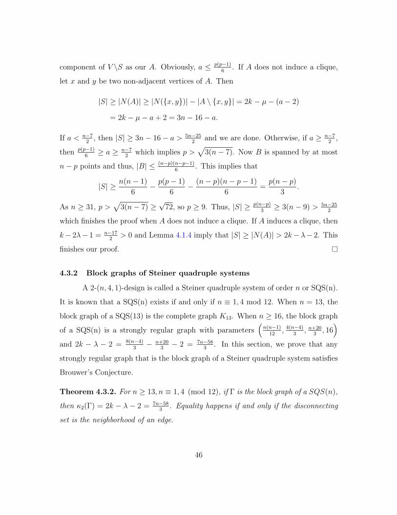
component of V \S as our A. Obviously, a ≤ p(p−1)6

. If A does not induce a clique,

let x and y be two non-adjacent vertices of A. Then

|S| ≥ |N(A)| ≥ |N({x, y})| − |A \ {x, y}| = 2k − µ− (a− 2)

= 2k − µ− a+ 2 = 3n− 16− a.

If a < n−72

, then |S| ≥ 3n− 16− a > 5n−252

and we are done. Otherwise, if a ≥ n−72

,

then p(p−1)6≥ a ≥ n−7

2which implies p >

√3(n− 7). Now B is spanned by at most

n− p points and thus, |B| ≤ (n−p)(n−p−1)6

. This implies that

|S| ≥ n(n− 1)

6− p(p− 1)

6− (n− p)(n− p− 1)

6=p(n− p)

3.

As n ≥ 31, p >√

3(n− 7) ≥√

72, so p ≥ 9. Thus, |S| ≥ p(n−p)3≥ 3(n− 9) > 5n−25

2

which finishes the proof when A does not induce a clique. If A induces a clique, then

k− 2λ− 1 = n−172

> 0 and Lemma 4.1.4 imply that |S| ≥ |N(A)| > 2k−λ− 2. This

finishes our proof.

4.3.2 Block graphs of Steiner quadruple systems

A 2-(n, 4, 1)-design is called a Steiner quadruple system of order n or SQS(n).

It is known that a SQS(n) exists if and only if n ≡ 1, 4 mod 12. When n = 13, the

block graph of a SQS(13) is the complete graph K13. When n ≥ 16, the block graph

of a SQS(n) is a strongly regular graph with parameters(n(n−1)

12, 4(n−4)

3, n+20

3, 16)

and 2k − λ − 2 = 8(n−4)3− n+20

3− 2 = 7n−58

3. In this section, we prove that any

strongly regular graph that is the block graph of a Steiner quadruple system satisfies

Brouwer’s Conjecture.

Theorem 4.3.2. For n ≥ 13, n ≡ 1, 4 (mod 12), if Γ is the block graph of a SQS(n),

then κ2(Γ) = 2k − λ − 2 = 7n−583

. Equality happens if and only if the disconnecting

set is the neighborhood of an edge.

46

Proof. When n = 13, the block graph of a SQS(13) is the complete graph K13 which

is OK. When n = 16, the SRG is a complete multipartite graph with parameters

(20, 16, 12, 16). By [31, Lemma 2.1], this graph is OK. Assume that 25 ≤ n ≤ 126.

Suppose first that 3 ≤ a ≤ 5. We have two possible cases:

1. The set A contains three vertices x, y and z that form a triangle. We consider

two subcases depending on whether or not the blocks of x, y, z have nonempty

intersection.

(a) The three blocks of x, y and z intersect in one point. We may assume that

x = {1, 2, 3, 4}, y = {1, 5, 6, 7}, z = {1, 8, 9, 10}. Then x, y and z have at

least n−103≥ 5 common neighbors.

(b) The three blocks of x, y and z have an empty intersection. For 1 ≤ u 6= v ≤

n, denote by {u, v, ∗, ∗} the block of the Steiner system containing u and

v. We may assume that x = {1, 2, 3, 4}, y = {2, 5, 6, 7}, z = {1, 5, 8, 9}.

Then x, y and z have at least 6 common neighbors: {1, 6, ∗, ∗},{1, 7, ∗, ∗},

{2, 8, ∗, ∗}, {2, 9, ∗, ∗}, {3, 5, ∗, ∗}, {4, 5, ∗, ∗}.

By inclusion and exclusion, we obtain that

|S| ≥ |N(A)| ≥ |N({x, y, z})| − (a− 3)

≥ [3(k − 2)− 3(λ− 1) + 5]− 2

= 3n− 36 ≥ 7n− 58

3.

If the equality holds, then n = 25, a = 5, b = 6 and s = 39. However, Lemma

4.1.2 implies that

|S| ≥ 4× 5× 6× 16

(15− 16)2 + 4× (28− 16)≈ 39.1836 (4.6)

which is a contradiction that finishes the proof of this subcase.

47

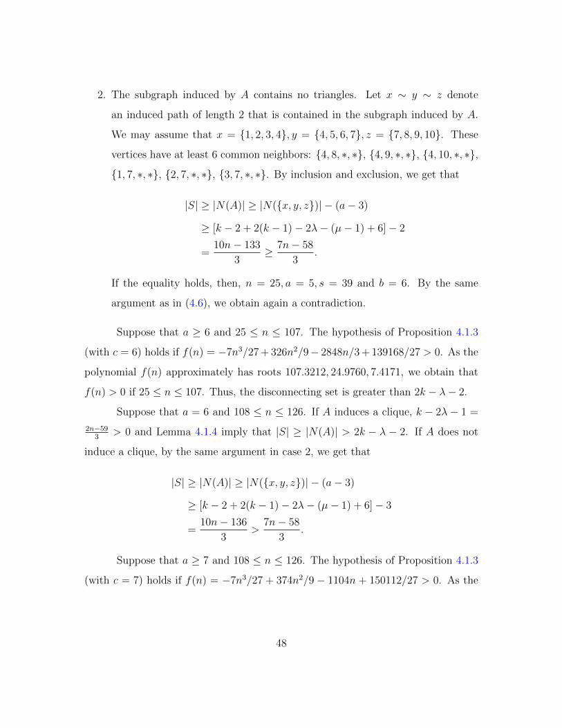
2. The subgraph induced by A contains no triangles. Let x ∼ y ∼ z denote

an induced path of length 2 that is contained in the subgraph induced by A.

We may assume that x = {1, 2, 3, 4}, y = {4, 5, 6, 7}, z = {7, 8, 9, 10}. These

vertices have at least 6 common neighbors: {4, 8, ∗, ∗}, {4, 9, ∗, ∗}, {4, 10, ∗, ∗},

{1, 7, ∗, ∗}, {2, 7, ∗, ∗}, {3, 7, ∗, ∗}. By inclusion and exclusion, we get that

|S| ≥ |N(A)| ≥ |N({x, y, z})| − (a− 3)

≥ [k − 2 + 2(k − 1)− 2λ− (µ− 1) + 6]− 2

=10n− 133

3≥ 7n− 58

3.

If the equality holds, then, n = 25, a = 5, s = 39 and b = 6. By the same

argument as in (4.6), we obtain again a contradiction.

Suppose that a ≥ 6 and 25 ≤ n ≤ 107. The hypothesis of Proposition 4.1.3

(with c = 6) holds if f(n) = −7n3/27 + 326n2/9− 2848n/3 + 139168/27 > 0. As the

polynomial f(n) approximately has roots 107.3212, 24.9760, 7.4171, we obtain that

f(n) > 0 if 25 ≤ n ≤ 107. Thus, the disconnecting set is greater than 2k − λ− 2.

Suppose that a = 6 and 108 ≤ n ≤ 126. If A induces a clique, k − 2λ − 1 =

2n−593

> 0 and Lemma 4.1.4 imply that |S| ≥ |N(A)| > 2k − λ − 2. If A does not

induce a clique, by the same argument in case 2, we get that

|S| ≥ |N(A)| ≥ |N({x, y, z})| − (a− 3)

≥ [k − 2 + 2(k − 1)− 2λ− (µ− 1) + 6]− 3

=10n− 136

3>

7n− 58

3.

Suppose that a ≥ 7 and 108 ≤ n ≤ 126. The hypothesis of Proposition 4.1.3

(with c = 7) holds if f(n) = −7n3/27 + 374n2/9 − 1104n + 150112/27 > 0. As the

48

polynomial f(n) approximately has roots 128.4292, 25.2414, 6.6152, we obtain that

f(n) > 0 if 108 ≤ n ≤ 126. Thus, the disconnecting set is greater than 2k − λ− 2.

Now, assume that n ≥ 127. Let p denote the number of points contained in the

blocks corresponding to the vertices of A. We may assume that p ≤ n−p. Otherwise,

we can choose some other component of V \S as our A. Obviously, a ≤ p(p−1)12

. If A

does not induce a clique, let x and y be two non-adjacent vertices of A. Then

|S| ≥ |N(A)| ≥ |N({x, y})| − |A \ {x, y}| = 2k − µ− (a− 2)

= 2k − µ− a+ 2 =8n− 74

3− a.

If a < n−163

, then |S| ≥ 8n−743− a > 7n−58

3and we are done. Otherwise, if a ≥ n−16

3,

then p(p−1)12≥ a ≥ n−16

3which implies p >

√2(n− 16). Now B is spanned by at

most n− p points and thus, |B| ≤ (n−p)(n−p−1)12

. This implies

|S| ≥ n(n− 1)

12− p(p− 1)

12− (n− p)(n− p− 1)

12

=p(n− p)

6≥√

2(n− 16)(n−√

2(n− 16))

6.

Now

√2(n−16)(n−

√2(n−16))

6> 7n−58

3is equivalent to f(n) = n3 − 144n2 + 2368n −

10952 > 0. It is true when n ≥ 126. Thus, |S| > 7n−583

in this case. If A induces a

clique, k−2λ−1 = 2n−593

> 0 and Lemma 4.1.4 imply that |S| ≥ |N(A)| > 2k−λ−2

which finishes our proof.

4.4 Brouwer’s Conjecture for Latin Square Graphs

Recall that an orthogonal array OA(t, n) with parameters t and n is a t× n2

matrix with entries from the set [n] = {1, . . . , n} such that the n2 ordered pairs

defined by any two distinct rows of the matrix are all distinct. It is well known that

an orthogonal OA(t, n) is equivalent to the existence of t − 2 mutually orthogonal

49

Latin squares (see [56, Section 10.4]). Given an orthogonal array OA(t, n), one can

define a graph Γ as follows: The vertices of Γ are the n2 columns of the orthogonal

array and two distinct columns are adjacent if they have the same entry in one

coordinate position. The graph Γ is an (n2, t(n− 1), n− 2 + (t− 1)(t− 2), t(t− 1))-

SRG.

When t = 2 and n 6= 4, such a graph must be the line graph of Kn,n which

is also the graph associated with an orthogonal array OA(2, n) (see [76, Problem

21F]); this graph is OK by [31, Section 8]. When t = 2 and n = 4, there are two

strongly regular graphs with parameters (16, 6, 2, 2), the line graph of K4,4 and the

Shrikhande graph (see [18, p. 125]); they are both OK by [31, Section 10].

The following theorem is the main result of this section and it shows that

Latin square graphs with parameters (n2, t(n − 1), n − 2 + (t − 1)(t − 2), t(t − 1))

satisfy Brouwer’s Conjecture when n ≥ 2t ≥ 6. In particular, this will imply that

strongly regular graphs obtained from orthogonal arrays OA(t, n) satisfy Brouwer’s

Conjecture when n ≥ 2t ≥ 6.

Theorem 4.4.1. Let t ≥ 3 be an integer. For any n ≥ 2t, if Γ is an (n2, t(n −

1), n− 2 + (t− 1)(t− 2), t(t− 1))-SRG, then

κ2(Γ) = 2k − λ− 2 = (2t− 1)n− t2 + t− 2.

The only disconnecting set of size (2t − 1)n − t2 + t − 2 are of the form N({uv}),

where u and v are two adjacent vertices in Γ.

Proof. IfA induces a clique in Γ, then the inequality k−2λ−1 = (t−2)n−2t2+5t−1 ≥

(t− 2)(2t)− 2t2 + 5t− 1 = t− 1 and Lemma 4.1.4 imply that |S| > 2k − λ− 2.

If A does not induce a clique in Γ, then A must contain an induced path

of length 2. By inclusion and exclusion, we deduce that a + s ≥ 3k − 2λ − µ =

50

(3t−2)n−3t2+4t. Assume by contradiction that s ≤ 2k−λ−2 = (2t−1)n−t2+t−2.

Then b ≥ a ≥ k − λ− µ+ 2 ≥ (t− 1)(n− 2t+ 1) + 3. Combining these inequalities

with a+ b = v − s ≥ n2 − (2t− 1)n+ t2 − t+ 2, we get ab ≥ [(t− 1)(n− 2t+ 1) +

3][n2 − (3t− 2)n+ 3t2 − 4t]. By Lemma 4.1.2, we have

s ≥ 4t(t− 1)[(t− 1)(n− 2t+ 1) + 3][n2 − (3t− 2)n+ 3t2 − 4t]

n2. (4.7)

Note that n2 − (3t − 2)n + 3t2 − 4t ≥ n2

4. This is because for any fixed t ≥ 3,

the function g(n) = 3n2 − (12t − 8)n + 12t2 − 16t is increasing in [2t,∞]. Thus,

g(n) ≥ g(2t) = 0. Using this fact in inequality (4.7), we obtain that

s ≥ t(t− 1)[(t− 1)(n− 2t+ 1) + 3]. (4.8)

Let f(n) = t(t − 1)[(t − 1)(n − 2t + 1) + 3] − [(2t − 1)n − t2 + t − 2]. When t ≥ 3,

f(n) is increasing in [2t,∞]. Thus,

f(n) ≥ f(2t) = t(t− 1)(t+ 2)− (3t2 − t− 2)

> t(t− 1)(t+ 2)− 3t2

= t(t2 − 2t− 2) > 0.

Combining with inequality (4.8), we have s > (2t − 1)n − t2 + t − 2. This is a

contradiction that finishes our proof.

The following consequence of Theorem 5.4.5 extends Lemma 9.1 from [31].

Corollary 4.4.2. For t ∈ {3, 4} and any integer n ≥ t, any strongly regular graph

associated with an OA(t, n) satisfies Brouwer’s Conjecture.

Proof. For t = 3, we need to see what happens when n ∈ {3, 4, 5}. If n = 3, the

corresponding graph is the complete three-partite graph K3,3,3 which is OK by [31,

51

Lemma 2.1]. If n = 4, the corresponding graph is a (16, 9, 4, 6)-SRG which is OK by

[31, Lemma 2.1]. If n = 5, the corresponding graph is a (25, 12, 5, 6)-SRG which is

OK by [31, Lemma 2.5].

For t = 4, we need to check what happens when n ∈ {4, 5, 6, 7}. If n = 4, the

corresponding graph is the complete four-partite graph K4,4,4,4 which is OK by [31,

Lemma 2.1]. If n = 5, the corresponding graph is a (25, 16, 9, 12)-SRG is OK by [31,

Lemma 2.1]. If n = 6, as shown by Tarry (see also Stinson [98]) an orthogonal array

OA(4, 6) does not exist. We remark here that McKay and Spence proved that there

are exactly 32458 strongly regular graphs with parameters (36, 20, 10, 12). If n = 7,

the corresponding graph is a (49, 24, 11, 12)-SRG which is OK [31, Lemma 2.5].

4.5 The Edge Version of Brouwer’s Conjecture

In this section, we give a short proof of the edge version of Brouwer’s Con-

jecture. We remark here that similar results were obtained by Hamidoune, Llado,

Serra and Tindell [61] for some families of vertex-transitive graphs.

Theorem 4.5.1. Let Γ be a connected (v, k, λ, µ)-SRG. If A is a subset of vertices

with 2 ≤ |A| ≤ v/2, then

e(A,Ac) ≥ 2k − 2. (4.9)

Equality happens if and only if A consists of two adjacent vertices or A induces a

triangle in K2,2,2 or A induces a triangle in the line graph of K3,3.

Proof. If k = 3, then Γ is K3,3 or the Petersen graph. If Γ is K3,3, the proof is

immediate. If Γ is the Petersen graph, and A is a subset of vertices with 3 ≤

|A| ≤ 4, then the number of edges contained in A is at most |A| − 1 and therefore

e(A,Ac) ≥ 3|A| − 2(|A| − 1) = |A| + 2 ≥ 5. If |A| = 5, then the number of edges

inside A is at most |A| = 5 and therefore e(A,Ac) ≥ 3|A| − 2|A| = |A| = 5. If k = 4,

52

then Γ is K4,4, K2,2,2 or the line graph of K3,3. If Γ is K4,4, the proof is immediate.

If Γ is K2,2,2, and A is a subset of 3 vertices inducing a triangle, then e(A,Ac) = 6;

in all the other cases, e(A,Ac) > 6. If Γ is the line graph of K4,4 and A is a subset

of vertices with |A| = 3, then e(A,Ac) ≥ 6 with equality if and only if A induces a

clique of order 3. If |A| = 4, then the number of edges contained in A is at most 4

and therefore, e(A,Ac) ≥ 4|A| − 8 = 8.

Assume k ≥ 5. If 3 ≤ |A| ≤ k−2, then e(A,Ac) ≥ |A|(k+1−|A|) ≥ 3(k−2) >

2k − 2 as k ≥ 5. If k − 1 ≤ |A| ≤ v/2, then e(A,Ac) ≥ (k−θ2)a(v−a)v

≥ (k−θ2)(k−1)2

(by Theorem 1.4.1). If Γ is a conference graph of parameters (4t + 1, 2t, t − 1, t),

then k − θ2 = 4t+1−√

4t+12

> 4 for t ≥ 3. These inequalities imply that e(A,Ac) >

2(k − 1) which finishes the proof of this case. If Γ is not a conference graph and

k − θ2 > 4, then e(A,Ac) > 2k − 2 and we are done again. The only case left is

when Γ is not a conference graph and k − θ2 ≤ 4. In this case, the eigenvalues

of Γ are integers, θ2 ≥ k − 4 and θv ≤ −2 as Γ is not a complete graph. Since

k − 1 ≥ k − µ = θ2(−θv) ≥ 2k − 8, we get 5 ≤ k ≤ 7. If θv = −2, then by Theorem

3.3.1, Γ must have parameters (16, 6, 2, 2) and eigenvalue 6, 2 and −2. In this case,

e(A,Ac) ≥ (k−θ2)a(v−a)v

= a(16−a)4

> 10 for k − 1 = 5 ≤ a ≤ 8 = v/2. If θv ≤ −3, then

we obtain k − 1 ≥ k − µ = θ2(−θv) ≥ 3k − 12 which implies k = 5. In this case, the

graph Γ is the folded 5-cube which has parameters (16, 5, 0, 2) and eigenvalues 5, 1

and −3. As before, e(A,Ac) ≥ (k−θ2)a(v−a)v

= a(16−a)4

> 8 for 3 ≤ a ≤ 8. This finishes

our proof.

4.6 Remarks

Recall that, by Theorem 3.4.1, with finitely many exceptions, the strongly

regular graphs with smallest eigenvalue −m are of one of the following types:

(a) Complete multipartite graphs with classes of size m,

53

(b) Block graphs of Steiner m-systems with parameters(n(n− 1)

m(m− 1),m(n−m)

m− 1, (m− 1)2 +

n− 1

m− 1− 2,m2

),

(c) Latin square graphs with parameters

(n2,m(n− 1), n− 2 + (m− 1)(m− 2),m(m− 1)).

For any fixed integer m ≥ 3, the graphs in case (a) satisfy Brouwer’s Con-

jecture by [31, Lemma 2.1]. By our results in Section 4.3 and Section 4.4, all but

finitely many strongly regular graphs of type (b) or (c), satisfy Brouwer’s Conjec-

ture. This means that there are finitely many strongly regular graphs with smallest

eigenvalue −m that might not satisfy Brouwer’s Conjecture. When m = 2, Cioaba,

Kim and Koolen [31] proved that among the strongly regular graphs with smallest

eigenvalue −2, the only counterexamples of Brouwer’s Conjecture are the triangular

graphs T (m), where m ≥ 6. By Theorem 4.3.1, Theorem 4.3.2 and Corollary 4.4.2,

we know that when m = 3, 4, the strongly regular graphs of type (b) and (c) satisfy

Brouwer’s Conjecture.

We performed a computer search among feasible parameter sets of strongly

regular graphs with smallest eigenvalue −3 or −4 for parameter sets (v, k, λ, µ) that

do not satisfy the hypothesis of Proposition 2.4 in [31]. When m = 3, there are 321

such parameters that are the same as the parameters of block graphs of Steiner triple

systems and 66 other parameter sets. The smallest strongly regular graph with other

parameter sets is a (36, 21, 12, 12)-SRG. Therefore, the status of Brouwer’s Conjec-

ture is established for all strongly regular graphs with minimum eigenvalue −3 with

the exception of 387 possible parameters. When m = 4, there are 1532 parameters

that are the same as the parameters of block graphs of Steiner quadruple system

54

graphs and 232 other parameters. The smallest strongly regular graph with other

parameter sets is a (45, 32, 22, 24)-SRG. Thus, the status of Brouwer’s Conjecture

is established for all strongly regular graphs with minimum eigenvalue −4 with the

exception of 1764 possible parameter sets.

55

Chapter 5

THE EXTENDABILITY OF MATCHINGS IN STRONGLYREGULAR GRAPHS

Most of the results of this chapter have appeared in Cioaba and Li [36].

5.1 Introduction

A set of edgesM of a graph Γ is a matching if no two edges ofM share a vertex.

A matching M is perfect if every vertex is incident with exactly one edge of M . A

matching is near perfect if all but one of the vertices of Γ are incident with edges of

the matching. A graph Γ of even order v is called t-extendable if it contains at least

one perfect matching, t < v/2 and any matching of size t is contained in some perfect

matching. Graphs that are 1-extendable are also called matching covered (see Lovasz

and Plummer [80, page 113]). A graph Γ of odd order v is called t-near-extendable

(or t12-extendable in the notation of Yu [106]) if it contains at least one near perfect

matching, t < (v− 1)/2 and for every vertex x, any matching of size t that does not

cover x is contained in some near perfect matching that misses x. Graphs that are

0-near-extendable are also called factor-critical or hypomatchable (see Lovasz and

Plummer [80, page 89]). The extendability of a graph Γ of even order is defined as

the maximum t < v/2 such that Γ is t-extendable; in this case, we say that the graph

Γ precisely t-extendable. The extendability of a graph Γ of odd order is the largest

t < (v−1)/2 such that Γ is t-near-extendable; in this case, we say that Γ is precisely

t-near-extendable. In this chapter, the notion of (precisely) t-extendable will be used

56

for graphs of even order and the notion of (precisely) t-near-extendable will refer to

graphs of odd order.

Motivated among other things by work of Lovasz [77] on canonical decom-

position of graphs containing perfect matchings, the notion of extendability was

introduced in 1980 by Plummer [90] for graphs of even order, was later extended to

graphs of odd order by Yu [106] and has attracted a lot of attention (see the surveys

[91, 92], the book [107] and the references therein). Zhang and Zhang [109] obtained

an O(mn) algorithm for determining the extendability of a bipartite graph Γ of order

n and size m. At present time, the complexity of determining the extendability of a

non-bipartite graph is unknown.

In this chapter, we study the extendability of primitive strongly regular graphs.

Brouwer and Mesner (Theorem 3.3.2) proved that the vertex-connectivity of any

connected strongly regular graph equals its valency. Plesnık [89] (or [79, Chapter

7, Problem 30]) showed that if Γ is a k-regular and (k − 1)-edge-connected graph

with an even number of vertices, then the graph obtained by removing any k − 1

edges of Γ, contains a perfect matching. It follows that every connected strongly

regular graph is 1-extendable. Holton and Lou [65] showed that strongly regular

graphs with certain connectivity properties are 2-extendable and conjectured that

all but a few strongly regular graphs are 2-extendable. Lou and Zhu [81] proved

this conjecture and showed that every connected strongly regular graph of valency

k ≥ 3 is 2-extendable with the exception (See Figure 5.2) of the complete 3-partite

graph K2,2,2 (the (6, 4, 2, 4)-SRG) and the Petersen graph (the (10, 3, 0, 1)-SRG). An-

other result worth mentioning is that any vertex-transitive graph is 1-extendable or

0-near-extendable (see [56, Theorem 3.5.1] or [80, Theorem 5.5.24]). For other re-

sults involving the extendability of vertex or edge-transitive graphs (with large cyclic

connectivity) see Aldred, Holton and Lou [1]. Many strongly regular graphs have

57

trivial automorphism groups and our techniques are different than the ones used for

vertex-transitive graphs.

Figure 5.1: The only two strongly regular graphs which are not 2-extendable. The

non-extendable matchings of size 2 are highlighted

In this chapter, we show that every connected (v, k, λ, µ)-SRG of valency

k ≥ 5 is 3-extendable with exception of the complete 4-partite graph K2,2,2,2 (the

(8, 6, 4, 6)-SRG), the complement of the Petersen graph (the (10, 6, 3, 4)-SRG) and

the Shrikhande graph (one of the two (16, 6, 2, 2)-srgs). We also prove that any

connected (v, k, λ, µ)-SRG with λ ≥ 1 is bk/3c-extendable when µ ≤ k/2 and dk+14e-

extendable when µ > k/2. This result is close to being best possible as we will

prove that many connected strongly regular graphs with valency k, λ ≥ 1 are not

dk/2e-extendable. On the other hand, we also determine the extendability of many

families of strongly regular graphs including Latin square graphs, block graphs of

Steiner systems, triangular graphs, lattice graphs and all known triangle-free strongly

regular graphs. For each graph of valency k that we considered, the extendability is

at least dk/2e − 1. We conjecture that this is true for all connected strongly regular

58

graphs of even order. We also obtain similar results for strongly regular graphs of

odd order.

5.2 Main Tools

In this section, we introduce the notation used in this chapter and describe

the main tools used in our proofs. Let o(Γ) denote the number of components of odd

order of a graph Γ. If S is a subset of vertices of Γ, then Γ−S denotes the subgraph of

Γ obtained by deleting the vertices in S. Let N(T ) denote the set of vertices outside

T that are adjacent to at least one vertex of T . When T = {x}, let N(x) = N({x}).

If x is a vertex of a strongly regular graph Γ, let N2(x) = V (Γ) \ ({x} ∪N(x)); the

first subconstituent Γ1(x) of x is the subgraph of Γ induced by N(x) and the second

subconstituent Γ2(x) of x is the subgraph of Γ induced by N2(x).

Theorem 5.2.1 (Tutte [100]). A graph Γ has a perfect matching if and only if

o(Γ− S) ≤ |S| for every S ⊂ V (Γ).

Theorem 5.2.2 (Gallai [53]). A graph Γ is factor-critical (or 0-near-extendable) if

and only if Γ has an odd number of vertices and o(Γ−S) ≤ |S| for all ∅ 6= S ⊂ V (Γ).

Using the above theorems, Yu [106] obtained the following characterizations

of graphs that are not t-extendable (resp. not t-near-extendable).

Lemma 5.2.3 (Yu [106]). Let t ≥ 1 and Γ be a graph containing a perfect matching.

The graph Γ is not t-extendable if and only if it contains a subset of vertices S such

that S contains t independent edges and o(Γ− S) ≥ |S| − 2t+ 2.

Lemma 5.2.4 (Yu [106]). Let t ≥ 1 and Γ be a factor-critical graph. The graph Γ

is not t-near-extendable if and only if it contains a subset of vertices S such that S

contains t independent edges, |S| ≥ 2t+ 1, and o(Γ− S) ≥ |S| − 2t+ 1.

59

Lemma 5.2.5. If Γ is a distance-regular graph of degree k ≥ 2 and diameter D ≥ 3,

then, for any x ∈ V (Γ), the subgraph induced by the vertices at distance 2 or more

from x is connected.

Proof. As D ≥ 3, Γ contains an induced path P4 with 4 vertices. By eigenvalue

interlacing, the second largest eigenvalue θ2(Γ) of Γ, is at least θ2(P4) = −1+√

52

> 0.

Cioaba and Koolen [32] proved that if the i-th entry of the standard sequence (See

[17, Page 128]) corresponding to the second largest eigenvalue of a distance-regular

graph Γ is positive, then for any vertex x, the subgraph of Γ induced by the vertices

at distance at least i from x is connected. The second entry of the standard sequence

corresponding to θ2(Γ) is θ2(Γ)/k > 0 and this finishes our proof.

Lemma 5.2.6. Let Γ be a (v, k, λ, µ)-SRG with λ ≥ 1. If T is an independent set,

then |N(T )| ≥ 2|T |.

Proof. For any x ∈ N(T ), N(x) ∩ T is an independent set in the subgraph Γ1(x)

which is induced by N(x). The subgraph Γ1(x) is λ-regular. Consider the edges in

Γ1(x). By counting the edges coming out of N(x)∩T , we get that |N(x)∩T |λ ≤ kλ/2

and thus, |N(x) ∩ T | ≤ k/2. Therefore, |T |k = e(T,N(T )) =∑

x∈N(T ) |N(x) ∩ T | ≤

|N(T )|k/2 implying |N(T )| ≥ 2|T |.

Lemma 5.2.7. Let Γ be a (v, k, λ, µ)-SRG. If T is an independent set, then

|N(T )| ≥ k2|T |k + |T |µ− µ

. (5.1)

Proof. For x ∈ N(T ), let dx = |T ∩ N(x)| and d =∑x∈N(T ) dx

|N(T )| . Counting the edges

between T and N(T ), we have |T |k = |N(T )|d. Counting the 3-subsets of the form

{x, y, z} such that x, y ∈ T, z ∈ N(T ), x ∼ z, y ∼ z, we get that(|T |2

)µ =

∑x∈N(T )

(dx2

)≥ |N(T )|

(d

2

). (5.2)

60

Combining these equations, we obtain that (|T |−1)µ ≥ k(

k|T ||N(T )| − 1

)which implies

the desired inequality |N(T )| ≥ k2|T |k+|T |µ−µ .

Note that the result of Lemma 5.2.7 is better than the one obtained by

applying Inclusion-Exclusion Principle |N(T )| = | ∪x∈T N(x)| ≥∑

x∈T |N(x)| −∑x 6=y∈T |N(x) ∩N(y)| = k|T | − µ

(|T |2

)when |T | ≥ 1 + k/µ.

Lemma 5.2.8. Let Γ be a primitive (v, k, λ, µ)-SRG with λ ≥ 1. If T is an indepen-

dent set, then

|N(T )| − |T | ≥

k − 1 if 1 ≤ |T | ≤ (k−µ)(k−1)µ

or if |T | ≥ k − 1.

(k−2)[k(k−1)−(k−3)µ](k−3)µ+k

otherwise.

(5.3)

Proof. Define f(x) = k2xµx+k−µ − x for x ≥ 1. Note that f(1) = f

((k−µ)(k−1)

µ

)= k− 1

and that f ′(x) = k2(k−µ)(µx+k−µ)2

− 1. Hence, x0 = k√k−µ−(k−µ)

µis the only critical point

of f(x). Since k − µ > 1, we deduce that 1 < x0 <(k−µ)(k−1)

µ. Also, f ′(x) > 0 for

x ∈ [1, x0) and f ′(x) < 0 for x > x0. This implies that |N(T )| − |T | ≥ f(|T |) ≥

f(1) = f(

(k−µ)(k−1)µ

)= k − 1 whenever 1 ≤ |T | ≤ (k−µ)(k−1)

µ. If |T | ≥ k − 1, Lemma

5.2.6 implies that |N(T )| − |T | ≥ |T | ≥ k − 1. If (k−µ)(k−1)µ

< |T | ≤ k − 2, then the

previous arguments and Lemma 5.2.7 imply that |N(T )|−|T | ≥ f(|T |) ≥ f(k−2) =

(k−2)[k(k−1)−(k−3)µ](k−3)µ+k

.

Note that if λ ≥ 1 and µ ≤ k/2, then Lemma 5.2.8 implies that

|N(T )| − |T | ≥ k − 1 (5.4)

for any independent set of vertices T .

The following lemma extends Theorem 5.1 of [33].

61

Lemma 5.2.9. Let Γ be a primitive (v, k, λ, µ)-SRG. If A is a subset of vertices with

3 ≤ |A| ≤ v/2 and Ac denotes its complement, then

e(A,Ac) ≥ 3k − 6. (5.5)

Proof. If k = 3, then Γ is K3,3 or the Petersen graph. If Γ is K3,3, the proof is

immediate. If Γ is the Petersen graph, and A is a subset of vertices with 3 ≤

|A| ≤ 4, then the number of edges contained in A is at most |A| − 1 and therefore

e(A,Ac) ≥ 3|A| − 2(|A| − 1) = |A| + 2 ≥ 5. If |A| = 5, then the number of edges

inside A is at most |A| = 5 and therefore e(A,Ac) ≥ 3|A| − 2|A| = |A| = 5. If k = 4,

then Γ is K4,4, K2,2,2 or the Lattice graph L2(3) which is the unique (9, 4, 1, 2)-SRG.

If Γ is K4,4 or K2,2,2, the proof is immediate. If Γ is the Lattice graph L2(3), and A

is a subset of vertices with |A| = 3, then e(A,Ac) ≥ 6 with equality if and only if A

induces a clique of order 3. If |A| = 4, then the number of edges contained in A is

at most 4 and therefore, e(A,Ac) ≥ 4|A| − 8 = 8.

Assume k ≥ 5. If |A| ≤ k − 2, then e(A,Ac) ≥ |A|(k − |A| + 1) ≥ 3(k − 2).

Assume |A| = k − 1. If every vertex of A has at least 3 neighbors outside A, then

e(A,Ac) ≥ 3(k − 1). Otherwise, there exists a vertex x ∈ A that has exactly 2

neighbors outside A. Therefore, e(N(x)∩Ac, A) ≥ 2+2(λ−1) = 2λ. Each vertex in

N(x) has k−λ− 1 neighbors outside {x}∪N(x). Thus, e(N(x)∩A, V (Γ) \ (N(x)∪

{x})) ≥ (k − 2)(k − λ − 1). Hence, e(A,Ac) ≥ (k − 2)(k − λ − 1) + 2λ ≥ 3(k − 2)

since λ ≤ k − 2.

If k ≤ |A| ≤ v/2, then e(A,Ac) ≥ (k−θ2)|A|(v−|A|)v

≥ (k−θ2)k2

(by Theorem

1.4.1). If Γ is a conference graph of parameters (4t + 1, 2t, t − 1, t), then k − θ2 =

4t+1−√

4t+12

> 6 for t ≥ 4 and consequently, e(A,Ac) > 3k. If t = 3, Γ has parameters

(13, 6, 2, 3) and therefore, e(A,Ac) ≥ (k−θ2)|A|(v−|A|)v

> (13−√

13)|A|(13−|A|)2·13

> 12. If Γ

is not a conference graph and k − θ2 ≥ 6, then e(A,Ac) ≥ 3k and we are done

62

again. The only case left is when Γ is not a conference graph and k − θ2 ≤ 5.

In this case, the eigenvalues of Γ are integers, θ2 ≥ k − 5 and θv ≤ −2 as Γ is

not a complete graph. Since k − 1 ≥ k − µ = θ2(−θv) ≥ 2k − 10, we get 5 ≤

k ≤ 9. If θv = −2, then by Seidel’s characterization of strongly regular graphs

with minimum eigenvalue −2 (see [19, Section 9.2] or [95]), there are three cases

to consider. If Γ is a (16, 6, 2, 2)-SRG, then its second largest eigenvalue is 2 and

e(A,Ac) ≥ (k−θ2)|A|(v−|A|)v

= |A|(16−|A|)4

≥ 15 for k = 6 ≤ |A| ≤ 8 = v/2. If Γ

is a (15, 8, 4, 4)-SRG, then since k > v/2, |A| ≤ k − 1 and e(A,Ac) ≥ 3k − 6 by

a previous case. If Γ is a (25, 8, 3, 2)-SRG, then its second largest eigenvalue is 3

and e(A,Ac) ≥ (k−θ2)|A|(v−|A|)v

= |A|(25−|A|)5

≥ 24 for k = 8 ≤ |A| ≤ 12 = bv/2c.

If θv ≤ −3, then we obtain k − 1 ≥ k − µ = θ2(−θv) ≥ 3k − 15 which implies

5 ≤ k ≤ 7. If k = 5, then Γ is a (16, 5, 0, 2)-SRG whose second largest eigenvalue is

1. Thus, e(A,Ac) ≥ (k−θ2)|A|(v−|A|)v

= |A|(16−|A|)4

≥ 13 for k = 5 ≤ |A| ≤ 8 = bv/2c.

If k = 6, then Γ is a (15, 6, 1, 3)-SRG whose second largest eigenvalue is 1. Thus,

e(A,Ac) ≥ (k−θ2)|A|(v−|A|)v

= |A|(15−|A|)3

≥ 18 for k = 6 ≤ |A| ≤ 7 = bv/2c. If

k = 7, then Γ is a (50, 7, 0, 1)-SRG whose second largest eigenvalue is 2. Therefore,

e(A,Ac) ≥ (k−θ2)|A|(v−|A|)v

= |A|(50−|A|)10

≥ 28 for k = 7 ≤ |A| ≤ 25 = v/2. This finishes

our proof.

Lemma 5.2.10. If Γ is a (v, k, λ, µ)-SRG of even order with independence number

2, then the extendability of Γ is dk2e − 1.

Proof. The fact that the extendability is at least dk2e − 1 follows from Lemma 5.2.3.

If Γ is imprimitive, then Γ must be K2×m for some m and the conclusion will follow

from Section 3.1. Assume that Γ is primitive and α(Γ) = 2. For any vertex x ∈ V , let

N2(x) = V (Γ) \ ({x} ∪N(x)). The second subconstituent Γ2(x) must be a complete

graph with k − µ + 1 vertices. As the clique number is at most λ + 2, we have

63

θ2(−θv) = k − µ ≤ λ + 1. Since θv ≤ −2, we obtain that θ2 ≤ λ+12≤ λ − 1 (when

λ ≥ 3). The first subconstituent Γ1(x) is λ-regular with second largest eigenvalue

at most θ2. By [30], Γ1(x) contains a matching of size bk/2c. If k is even, then this

matching cannot be extended to a maximum matching of Γ. If k is odd, one can add

one disjoint edge to this matching such that the result matching of size dk2e cannot

be extended to a maximum matching of Γ. It is easy to see that when λ is 1 or 2,

Γ1(x) contains a perfect matching or an almost perfect matching.

Lemma 5.2.11. If Γ is a primitive (v, k, λ, µ)-SRG of even order with independence

number α(Γ) ≥ 3, then the extendability of Γ is at least dk+32− α(Γ)

2e − 1 ≥ dk+3

2−

v2(1+k/(−θv))

e − 1.

Proof. Let t = dk+32− α(Γ)

2e − 1. Assume that Γ is not t-extendable. By Lemma

5.2.3, there is a vertex disconnecting set S containing t independent edges, such that

o(Γ−S) ≥ |S|−2t+2 ≥ k−2t+2 ≥ 3. Because Γ is primitive, Theorem 3.3.2 implies

that |S| ≥ k + 1. Thus, α(Γ) ≥ o(Γ− S) ≥ |S| − 2t + 2 ≥ k − 2t + 3, contradiction

with t = dk+32− α(Γ)

2e − 1. The second part follows from the Hoffman-ratio bound

(Theorem 1.3.4) stating that α(Γ) ≤ v1+k/(−θv)

.

Lemma 5.2.12. If Γ is a (v, k, λ, µ)-SRG with λ = 0, then v > 3α(Γ) except when

Γ is the Petersen graph.

Proof. The Hoffman-ratio bound (Theorem 1.3.4) states that α(Γ) ≤ v1+k/(−θv)

. As

θ2(−θv) = k−µ < k, when θ2 ≥ 2, we have k/(−θv) > 2, thus α(Γ) < v/3. If θ2 = 1,

then θv = µ − k and −µ = λ − µ = θ2 + θv = 1 + µ − k. Thus, k = 2µ + 1 and

v = 1 + k + k(k − 1)/µ = 3k + 1 = 6µ + 4. Let f be the multiplicity of θ2 and g

be the multiplicity of θv. We have 1 + f + g = v and k + f + (µ − k)g = 0 and

therefore, v = 1− k + (k − µ+ 1)g. Hence, g = 8µ+4µ+2

= 8− 12µ+2

. As g is an integer,

64

µ ∈ {1, 2, 4, 10}. When µ = 4 or 10, we get v > g(g + 3)/2, which is impossible by

Seidel’s absolute bound (see [19, Section 9.1.8] or [45]). When µ = 1, Γ must be the

Petersen graph, where α(Γ) = 4 and v = 10 ≤ 3α(Γ) = 12. Finally, when µ = 2, Γ

is the (16, 5, 0, 2)-SRG, where 16 = v > 3α(Γ) = 15.

Lemma 5.2.13. Let Γ be a (v, k, λ, µ)-SRG with v even, λ = 0 and k ≥ 7. If A is a

subset of vertices such that 5 ≤ |A| ≤ v−k−1 and |A| is odd, then e(A,Ac) ≥ 5k−12.

Proof. Assume that 5 ≤ |A| ≤ 2k − 5. As Γ is triangle-free, so is the subgraph

induced by A. By Turan’s Theorem, the number of edges inside A is at most |A|2−14

.

So, e(A) ≤ |A|2−14

and e(A,Ac) = k|A| − 2e(A) ≥ k|A| − |A|2−12

. The minimum is

attained at |A| = 5 or 2k − 5. In either case, we have e(A,Ac) ≥ 5k − 12.

Assume that 2k − 3 ≤ |A| ≤ v/2. We have e(A,Ac) ≥ (k−θ2)|A|(v−|A|)v

≥(k−θ2)(2k−3)

2(by Theorem 1.4.1). Since θ2(−θv) = k − µ ≤ k − 1 and θv ≤ −3 when

k ≥ 7, we have θ2 ≤ k−13

and k − θ2 ≥ 2k+13

. So, when k ≥ 7, k − θ2 ≥ 5 and

e(A,Ac) ≥ 5(2k−3)2

> 5k − 12.

Assume that v/2 < |A| ≤ v−k−1. It is equivalent to that k+1 ≤ |Ac| < v/2.

We can apply the same argument to Ac and show that e(A,Ac) ≥ 5k − 12.

Lemma 5.2.14. Let Γ be a primitive (v, k, λ, µ)-SRG and S be a disconnecting set

of vertices. If Γ− S contains at least two singleton components, then S contains at

least µ(k − µ) edges.

Proof. Let x and y be two singleton components of Γ− S. Then N(x) ∪N(y) ⊆ S.

If z ∈ N(x) \N(y), then z and y are non adjacent and they have exactly µ common.

So, z is adjacent to at least µ vertices of S, and there are |N(x)\N(y)| = k−µ such

z. By the same argument, each vertex inside N(y) \ N(x) is adjacent to at least µ

vertices of S. Thus, 2e(S) ≥ 2µ(k − µ).

65

5.3 The Extendability of Strongly Regular Graphs

5.3.1 Imprimitive strongly regular graphs

Recall that a strongly regular graph is imprimitive if it, or its complement,

is disconnected. The only imprimitive strongly regular graphs are disjoint unions

of cliques of the same order and their complements (complete multipartite regular

graphs). A disjoint union mKa of some number m ≥ 2 of cliques Ka does not

contain a perfect matching nor a near perfect matching if a is odd. If a is even,

the extendability of this graph is am/2− 1. The complete multipartite graph Ka×m

(which is the complement of mKa) has extendability am/2 − 1 if m = 2. When

m ≥ 3, if am is even, the extendability of Ka×m is a(m−2)2

= k−a2

and if am is odd,

the extendability of Ka×m is a(m−2)−12

= bk−a2c.

5.3.2 Lower bounds for the extendability of strongly regular graphs

In this section, we classify the primitive strongly regular graphs of even order

that are not 3-extendable. We first provide results giving some general lower bounds

for the extendability of a primitive strongly regular graphs.

Theorem 5.3.1. If Γ is a (v, k, λ, µ)-SRG with k/2 < µ < k and α(Γ) ≥ 3, then

the extendability of Γ is at least max(dk+3

2− 3k−2λ−3

2(2θ2+1)e − 1, dλ/2 + 1e

).

Proof. Since µ > k/2, we get that v = 1 + k + k(k − λ− 1)/µ < 3k − 2λ− 1. Also,

µ > k/2 implies that Γ has integer eigenvalues and θ2(−θv) = k − µ < k/2. By

the Hoffman-ratio bound (Theorem 1.3.4), α(Γ) ≤ v1+k/(−θv)

< v1+2θ2

. Combining

these inequalities, we get that α(Γ) ≤ 3k−2λ−31+2θ2

. The second subconstituent Γ2(x) is

connected (see [19, Proposition 9.3.1]) and |N2(x)| = k(k− λ− 1)/µ < 2(k− λ− 1).

Thus, α(Γ) ≤ 1 + |N2(x)|2

which implies α(Γ) ≤ k − λ − 1. By Lemma 5.2.11, the

extendability of Γ is at least max(dk+3

2− 3k−2λ−3

2(2θ2+1)e − 1, dλ/2 + 1e

).

66

Note that the bounds in Theorem 5.3.1 are incomparable. When θ2 = 1, the

first bound gives us dλ/3 + 1e and the second bound dλ/2 + 1e is better. On the

other hand, when λ = k/2 and θ2 ≥ 2, the first bound gives us d3k/10 + 4/5e which

is better than the second bound dk/4 + 1e. There exist strongly regular graphs with

λ = k/2 and θ2 ≥ 2, for example, the (36, 20, 10, 12)-SRG.

Corollary 5.3.2. Any primitive (v, k, λ, µ)-SRG with µ > k/2 and k ≥ 8 is 3-

extendable.

Proof. If θ2 ≥ 2, then θv = µ−kθ2

> −k/4 as µ > k/2. Thus, λ = µ + θ2 + θv >

k/2 + 2−k/4 = k/4 + 2. By Theorem 5.3.1, the extendability is at least d2k+2λ+810e >

dk/4 + 1.2e ≥ 4 for k ≥ 8. If θ2 = 1, we will show that λ ≥ k−32

. The second bound

in Theorem 5.3.1 will then imply the extendability is at least dk+14e ≥ 3. Since

θ2 = 1, then −θv = k − µ, 1 + θv = λ − µ and consequently, λ = 2µ + 1 − k and

v = 1 + k + k(k−λ−1)µ

= 1 + k + 2k(k−µ−1)µ

. If 3k/4 ≤ µ < k, then λ ≥ k/2 + 1 > k−32

.

Otherwise, assume that k/2 < µ < 3k/4, and let f be the multiplicity of θ2 and

g be the multiplicity of θv. We have 1 + f + g = v and k + f + (µ − k)g = 0

and therefore, 1 − k + (k − µ + 1)g = v = 1 + k + 2k(k−µ−1)µ

. Hence, 2(k − 1)k =

g(k−µ+1)µ > g(1+k/4)(3k/4) (as (k−µ+1)µ attains minimum at µ = 3k/4) and

g < 32(k−1)3(k+4)

< 11. Thus, g ≤ 10. By Seidel’s absolute bound (see [19, Section 9.1.8] or

[45]), v < g(g+3)2≤ 65. We checked all the possible parameter sets of strongly regular

graphs with v even and θ2 = 1 from the list [16]. All of them have the property that

λ ≥ k−32

, and there is exactly one parameter set which attains the equality. It is the

(28, 15, 6, 10) and there are 4 such strongly regular graphs, the triangular graph T (8)

and the three Chang graphs (see Brouwer’s list [16] or [19, page 123]).

Note that Chen [29] proved the following theorem (see also Aldred and Plum-

mer [2] for extensions of Chen’s result).

67

Theorem 5.3.3 (Chen [29]). Let t ≥ 1 and n ≥ 2 be two integers. If Γ is a

(2t+ n− 2)-connected K1,n-free graph of even order, then Γ is t-extendable.

When λ ≥ 1, every (v, k, λ, µ)-SRG is k-connected and K1,bk/2c+1-free. If we

let t = b12dk+2

2ec and n = bk/2c + 1, then Chen’s result implies that such strongly

regular graph is b12dk+2

2ec-extendable. This is the same as our result when θ2 = 1,

µ > k/2 and λ ≤ k−32

. For other cases, our lower bound is better than Chen’s result.

Note that Chen’s bound can be improved if one has a better bound than k/2 for the

independence number of the first subconstituents of the strongly regular graph.

Theorem 5.3.4. Let Γ be a primitive (v, k, λ, µ)-SRG with λ ≥ 1. If µ ≤ k/2, then

Γ is n-extendable, where n = dk2−k−33k−7

e − 1.

Proof. If Γ is not n-extendable, by Lemma 5.2.3, there is a vertex set S with s

vertices such that S contains n independent edges, and Γ−S has at least s− 2n+ 2

odd components. Let O1, O2, . . . , Or be all the odd components of Γ − S, with

r ≥ s−2n+2. Let a ≥ 0 denote the number singleton components among O1, . . . , Or.

Counting the number of edges between S and O1 ∪ · · · ∪Or and using Lemma 5.2.9,

we get the following

ks−2n ≥ e(S,O1∪· · ·∪Or) ≥ ak+(r−a)(3k−6) ≥ ak+(s−2n+2−a)(3k−6). (5.6)

This inequality is equivalent to

n ≥ (k − 3)(s− a) + 3k − 6

3k − 7(5.7)

and since s− a ≥ k − 1 (see the remark following Lemma 5.2.8), we obtain that

n ≥ (k − 3)(k − 1) + 3k − 6

3k − 7=k2 − k − 3

3k − 7. (5.8)

This is a contradiction with n = dk2−k−33k−7

e − 1 < k2−k−33k−7

.

68

Corollary 5.3.5. Any primitive (v, k, λ, µ)-SRG with λ ≥ 1 and k ≥ 8 is 3-

extendable.

Proof. Note that dk2−k−33k−7

e− 1 = bk/3c if k ≡ 0, 1 (mod 3) and bk/3c+ 1, otherwise.

Corollary 5.3.2 and Theorem 5.3.4 imply that any primitive (v, k, λ, µ)-SRG with

λ ≥ 1 and k ≥ 8 is 3-extendable.

Theorem 5.3.6. Any primitive (v, k, λ, µ)-SRG with λ = 0 and k ≥ 8 is 3-extendable.

Proof. We show that Γ is 3-extendable by contradiction. Assume that Γ is not 3-

extendable. Lemma 5.2.3 implies that Γ has a vertex subset S, such that S contains

3 independent edges, and o(Γ− S) ≥ |S| − 4. Let S be such disconnecting set with

maximum size. We first claim that any non-singleton component of Γ − S cannot

induce a bipartite graph. If that was the case, the respective component would have

two partitions X and Y . Assume that |X| > |Y |, then define S ′ = S ∪ Y . Then

|S ′| > |S| and o(Γ−S ′) ≥ |S ′|−4, contradicting the maximality of |S|. Note that Γ−S

cannot contain exactly 3 vertices, because Γ is triangle free and any component with

3 vertices must be a path, which is bipartite. By similar argument, Γ−S contains no

even components. If it contains a even component, we can put one vertex of this even

component into S, which make |S| larger and S still satisfy o(Γ− S) ≥ |S| − 4. But

it contradicts to the maximality of |S|. Let O1, O2, . . . , Or be all the odd components

of Γ−S. If Γ−S has only singleton components, then α(Γ) ≥ o(Γ−S) ≥ |S| − 4 ≥

v − α(Γ) − 4. Thus, 3α(Γ) < v ≤ 2α(Γ) + 4 and k ≤ α(Γ) < 4, which contradicts

to k ≥ 8. If Γ− S has at most one singleton component, as o(Γ− S) ≥ |S| − 4 ≥ 3,

Γ−S has at least two non-singleton components, thus |S| ≥ k+ 1. By using Lemma

5.2.13 and counting the edges between S and O1∪ · · ·∪Or, we will get the following,

k|S| − 6 ≥ e(S,O1 ∪ · · · ∪Or) ≥ k + (|S| − 5)(5k − 12)

69

which implies that

12k − 33 ≥ (2k − 6)|S| ≥ (2k − 6)(k + 1).

Thus, 2k2 − 16k + 27 ≤ 0, contradiction with k ≥ 8.

If Γ−S has at least one non-singleton components and at least two singleton

components, by using Lemma 5.2.13 and Lemma 5.2.14 and counting the edges

between S and O1 ∪ · · · ∪Or, we will get that

k|S|−2(k−1) ≥ k|S|−2µ(k−µ) ≥ k|S|−2e(S) ≥ e(S,O1∪· · ·∪Or) ≥ 5k−12+(|S|−5)k

which will yield another contradiction with k ≥ 8.

Note that this theorem covers all known primitive triangle-free strongly reg-

ular graph with even order with precisely three exceptions. These are the Petersen

graph, which is the unique (10, 3, 0, 1)-SRG (and has extendability 1), the folded

5-cube, which is the unique (16, 5, 0, 2)-SRG (and has extendability 3; see Theorem

5.4.9) and the Hoffman-Singleton graph, which is the unique (50, 7, 0, 1)-SRG (and

has extendability 5; see Theorem 5.4.10).

Corollary 5.3.7. Let Γ be a primitive (v, k, λ, µ)-SRG with v even and k ≥ 5. Then

Γ is 3-extendable unless Γ is the complete 4-partite graph K2,2,2,2 (the (8, 6, 4, 6)-

SRG), the complement of the Petersen graph (the (10, 6, 3, 4)-SRG) or the Shrikhande

graph (one of the two (16, 6, 2, 2)-SRGs).

70

Figure 5.2: The three strongly regular graphs with k ≥ 6 which are not 3-

extendable. The non-extendable matchings of size 3 are highlighted.

Deleting the highlighted matching in each graph will isolate a vertex,

thus the remaining graph does not have a perfect matching.

Proof. If k ≥ 8, then Γ is 3-extendable by Corollary 5.3.5 and Theorem 5.3.6. There

are two primitive parameter sets with v even, λ ≥ 1 and 5 ≤ k ≤ 7: (10, 6, 3, 4) and

(16, 6, 2, 2). There is a unique (10, 6, 3, 4)-SRG, the complement of Petersen graph or

the triangular graph T (5). Proposition 5.4.2 will show that the extendability of this

graph is 2. There are two non-isomorphic strongly regular graphs with parameter set

71

(16, 6, 2, 2). One is the Shrikhande graph (see [19, page 123] for a description) and

the other is the line graph of K4,4. In the Shrikhande graph, the first subconstituent

of a fixed vertex is isomorphic to the cycle C6 and thus contains a matching of size

3. This matching is not contained in any perfect matching. Thus, the Shrikhande

graph is not 3-extendable; by Lou and Zhu [81], the extendability of the Shrikhande

graph is 2. Proposition 5.4.7 will show that the extendability of the line graph of

K4,4 is 3. To finish the proof, the only strongly regular graph with 5 ≤ k ≤ 7 and

λ = 0 is the folded 5-cube whose extendability is 3 (see Theorem 5.4.9).

The previous argument can be generalized to classify primitive 4-extendable

strongly regular graphs. By a more extensive case analysis which we omit here, we

can show that a primitive strongly regular graph Γ with even number of vertices

and λ ≥ 1 is 4-extendable if and only if k ≥ 9. Similarly, we can also classify all

the primitive 1-near-extendable and the 2-near-extendable strongly regular graphs.

When λ ≥ 1, every strongly regular graph of odd order is 1-near-extendable and

there is exactly one primitive strongly regular graph with λ ≥ 1 which is not 2-near-

extendable, namely the Paley graph on 9 vertices (the unique (9, 4, 1, 2)-SRG).

5.4 The Extendability of Some Specific Strongly Regular Graphs

In this section, we determine the extendability of several families of strongly

regular graphs. In the first three subsections, we show that there are many strongly

regular graphs with extendability equal or slightly larger than dk/2e − 1. In the

last subsection, we show that the extendability of any known triangle-free strongly

regular graph of even order and valency k equals k − 2.

The reason that the graphs considered in the next three subsections (except for

the graphs in Theorem 5.4.7) are not dk/2e-extendable (when v is even) or not k/2-

near-extendable (when v is odd) is the following. Consider the first subconstituent

72

Γ1(x) of any fixed vertex x; this is the subgraph induced by N(x). If v is even, we

will show that Γ1(x) has a matching of size k/2 if k is even and of size (k − 1)/2 if

k is odd. When k is odd, there is one vertex y not covered by the matching of size

(k − 1)/2 and we choose a vertex z not adjacent to x such that z is adjacent with

y. In each case, we construct a matching of size dk2e that cannot be contained in a

perfect since its removal leaves x isolated. If v is odd, then k is even. We will show

that Γ1(x) has a matching of size k/2. Choose a vertex y ∈ N2(x). The matching of

size k/2 in Γ1(x) does not cover y. Thus, we construct a matching that cannot be

contained in a near perfect matching that misses y since the removal of N(x) ∪ {y}

leaves x isolated. We will also use the following lemma.

Lemma 5.4.1. Let Γ be a graph of order am whose vertex set can be partitioned

into m subsets, A1, A2, . . . , Am with equal size a, such that for 1 ≤ i ≤ m, Ai induce

a clique, and the graph obtained by vertex contracting each Ai contains a perfect

matching (when m is even) or a near perfect matching (when m is odd). Then Γ

contains a perfect matching if am is even, and Γ contains a near perfect matching if

am is odd.

Proof. If a is even, the lemma is obvious. If a is odd and m is even, we can find a

matching u1u2, · · · , um−1um such that ui ∈ Ai for 1 ≤ i ≤ m. Now, each subgraph

induced by Ai\ui contain a perfect matching. Thus Γ contains a perfect matching. If

a is odd and m is odd, we can find a matching u1u2, · · · , um−2um−1 such that ui ∈ Aifor 1 ≤ i ≤ m−1. Now, each subgraph induced by Ai \ui contain a perfect matching

for 1 ≤ i ≤ m− 1 and Am contains a near perfect matching. Thus Γ contains a near

perfect matching.

73

5.4.1 Triangular graphs

Recall that the triangular graph T (m) is the line graph of the complete graph

Km; its vertices are the 2-subsets of [m] := {1, . . . ,m} and {u, v} ∼ {x, y} if and only

if |{u, v}∩{x, y}| = 1. The triangular graph T (m) is an ((m2

), 2(m−2),m−2, 4)-SRG.

Theorem 5.4.2. If m ≥ 4, the extendability of T (m) is k/2− 1 = m− 3.

Proof. We consider first the case when(m2

)is even. The subgraph induced by

N({1, 2}) contains a perfect matching; take {({1, i}, {2, i})|3 ≤ i ≤ m} for ex-

ample. By the observation at the beginning of Section 5.4, this shows that T (m) is

not (m− 2)-extendable.

Assume that T (m) is not (m − 3)-extendable. By Lemma 5.2.3, there is a

subset of vertices S such that S contains m − 3 independent edges and r = o(Γ −

S) ≥ |S| − 2(m − 3) + 2. Let O1, O2, . . . , Or be the odd components of Γ − S.

Denote by Pi the union of the 2-subsets corresponding to the vertices of Oi, for

1 ≤ i ≤ r. If r ≤ 3, then by Theorem 3.3.2, |S| ≥ 2(m − 2) and therefore,

3 ≥ o(Γ − S) ≥ |S| − 2(m − 3) + 2 ≥ 4, contradiction. If r ≥ 4, then since

P1, P2, . . . , Pr are disjoint subsets of [m], and |Pi| ≥ 2, we have m ≥ 8. There exists

two odd components, says O1, O2, such that 3 ≤ |P1 ∪ P2| ≤ m − 3. We have

{{u, v} | u ∈ P1 ∪P2, v ∈ [m]− (P1 ∪P2)} ⊂ N(O1 ∪O2) ⊂ S. Thus |S| ≥ 3(m− 3).

On the other hand, as 2r ≤ |P1| + |P2| + . . . + |Pr| ≤ m, we have r ≤ m/2. So,

m/2 ≥ o(Γ−S) ≥ |S|−2(m−3)+2 ≥ 3(m−3)−2(m−3)+2 = m−1, contradiction

with m ≥ 8.

If(m2

)is odd, by the same argument as above, it is easy to see that T (m) is

not (m− 2)-near-extendable. Assume that T (m) is not (m− 3)-near-extendable. By

Lemma 5.2.4, there is a subset of vertices S such that S contains m− 3 independent

edges, |S| ≥ 2(m− 3) + 1 and r = o(Γ− S) ≥ |S| − 2(m− 3) + 1. If r = 2, then by

74

Theorem 3.3.2, |S| ≥ 2(m− 2) and therefore, 2 = o(Γ−S) ≥ |S|− 2(m− 3) + 1 ≥ 3,

contradiction. If r = 3, S is not the neighborhood of some vertex. By Theorem

3.3.2, |S| ≥ 2(m − 2) + 1, and therefore, 3 = o(Γ − S) ≥ |S| − 2(m − 3) + 1 ≥ 4,

contradiction. The rest of the proof is the same as in the case(m2

)even.

5.4.2 Block graphs of Steiner systems

A 2-(n,K, 1)-design or a Steiner K-system is a point-block incidence structure

on n points such that each block has K points and any two distinct points are

contained in exactly one block. The block graph of such a Steiner system has as

vertices the blocks and two distinct blocks are adjacent if they intersect. The block

graph of a Steiner K-system is a(n(n−1)K(K−1)

, K(n−K)K−1

, (K − 1)2 + n−1K−1− 2, K2

)-SRG.

Theorem 5.4.3. Let Γ be the block graph of a Steiner K-system on n points such that

n(n−1)K(K−1)

is even. If K ∈ {3, 4} and n > K2 or K ≥ 5 and n > 4K2 + 5K + 24 + 96K−4

,

the extendability of Γ is dk/2e − 1, where k is the valency of Γ.

Proof. Let Γ be the block graph of Steiner K-system, and B denote the block sets

of the 2-(n,K, 1) design. Consider the neighborhood N({1, . . . , K}) of the vertex

{1, 2, . . . , K}. There is a partition of N({1, . . . , K}) into cliques, which is Ai = {b ∈

B | b ∩ {1, 2, . . . , K} = {i}} for 1 ≤ i ≤ K. For any Ai and Aj, there exist bi ∈ Aiand bj ∈ Aj such that n ∈ bi and n ∈ bj. So, bi and bj are adjacent. The graph

obtained by contracting each Ai is a complete graph. By Lemma 5.4.1, the first

subconstituent Γ1(x) contains a perfect matching or a near perfect matching. There

are dk/2e independent edges incident with all N(x) and not incident with x. This

implies Γ is not dk/2e-extendable.

Assume that Γ is not (dk/2e − 1)-extendable. By Lemma 5.2.3, there is a

subset of vertices S such that S contains dk/2e − 1 independent edges and r =

75

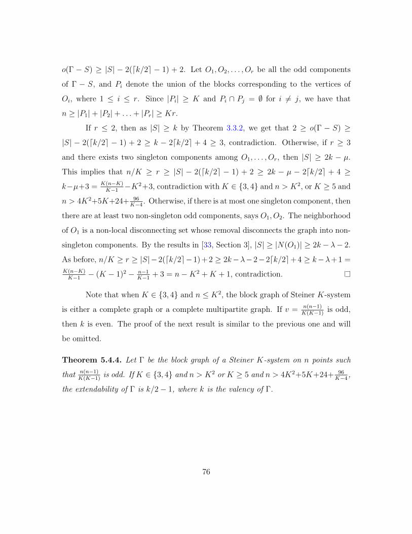
o(Γ − S) ≥ |S| − 2(dk/2e − 1) + 2. Let O1, O2, . . . , Or be all the odd components

of Γ − S, and Pi denote the union of the blocks corresponding to the vertices of

Oi, where 1 ≤ i ≤ r. Since |Pi| ≥ K and Pi ∩ Pj = ∅ for i 6= j, we have that

n ≥ |P1|+ |P2|+ . . .+ |Pr| ≥ Kr.

If r ≤ 2, then as |S| ≥ k by Theorem 3.3.2, we get that 2 ≥ o(Γ − S) ≥

|S| − 2(dk/2e − 1) + 2 ≥ k − 2dk/2e + 4 ≥ 3, contradiction. Otherwise, if r ≥ 3

and there exists two singleton components among O1, . . . , Or, then |S| ≥ 2k − µ.

This implies that n/K ≥ r ≥ |S| − 2(dk/2e − 1) + 2 ≥ 2k − µ − 2dk/2e + 4 ≥

k−µ+3 = K(n−K)K−1

−K2+3, contradiction with K ∈ {3, 4} and n > K2, or K ≥ 5 and

n > 4K2+5K+24+ 96K−4

. Otherwise, if there is at most one singleton component, then

there are at least two non-singleton odd components, says O1, O2. The neighborhood

of O1 is a non-local disconnecting set whose removal disconnects the graph into non-

singleton components. By the results in [33, Section 3], |S| ≥ |N(O1)| ≥ 2k− λ− 2.

As before, n/K ≥ r ≥ |S|−2(dk/2e−1) + 2 ≥ 2k−λ−2−2dk/2e+ 4 ≥ k−λ+ 1 =

K(n−K)K−1

− (K − 1)2 − n−1K−1

+ 3 = n−K2 +K + 1, contradiction.

Note that when K ∈ {3, 4} and n ≤ K2, the block graph of Steiner K-system

is either a complete graph or a complete multipartite graph. If v = n(n−1)K(K−1)

is odd,

then k is even. The proof of the next result is similar to the previous one and will

be omitted.

Theorem 5.4.4. Let Γ be the block graph of a Steiner K-system on n points such

that n(n−1)K(K−1)

is odd. If K ∈ {3, 4} and n > K2 or K ≥ 5 and n > 4K2+5K+24+ 96K−4

,

the extendability of Γ is k/2− 1, where k is the valency of Γ.

76

5.4.3 Latin square graphs

Recall that an orthogonal array OA(t, n) with parameters t and n is a t× n2

matrix with entries from the set [n] = {1, . . . , n} such that the n2 ordered pairs

defined by any two distinct rows of the matrix are all distinct. Given an orthogonal

array OA(t, n), one can define a graph Γ as follows. The vertices of Γ are the n2

columns of the orthogonal array and two distinct columns are adjacent if they have

the same entry in one coordinate position. The graph Γ is an (n2, t(n− 1), n− 2 +

(t − 1)(t − 2), t(t − 1))-SRG. Any strongly regular graph with such parameters is

called a Latin square graph. When t = 2 and n 6= 4, such a graph must be the line

graph of Kn,n which is also the graph associated with an orthogonal array OA(2, n)

(see [19, page 123]).

Theorem 5.4.5. Let n ≥ 2t ≥ 6 be two integers with n even. If Γ is a Latin square

graph corresponding to an OA(t, n), then the extendability of Γ is dk/2e − 1.

Proof. Let C denote the column set of the orthogonal array OA(t, n) corresponding

to Γ. Consider the neighborhood N(c1) of a column c1 = (c1(1), . . . , c1(t))T of C.

There is a partition of N(c1) into cliques, which is Ai = {c ∈ C | c(i) = c1(i)} for

1 ≤ i ≤ t. Let l ∈ [n] such that l 6= c1(3). There exist c ∈ A1 such that c(3) = l and

there is c′ ∈ A2 such that c′(3) = l. Thus c and c′ are adjacent. The graph obtained

by contracting each Ai is a complete graph. By Lemma 5.4.1 and the same argument

in Theorem 5.4.3, we deduce that Γ is not dk/2e-extendable.

Assume that Γ is not (dk/2e − 1)-extendable. By Lemma 5.2.3, there is a

subset of vertices S such that S contains dk/2e − 1 independent edges and r =

o(Γ− S) ≥ |S| − 2(dk/2e − 1) + 2. Let O1, O2, . . . , Or be all the odd components of

Γ− S.

77

If r ≤ 2, then as |S| ≥ k by Theorem 3.3.2, we have 2 ≥ r ≥ |S| − 2(dk/2e −

1) + 2 ≥ k− 2dk/2e+ 4 ≥ 3, contradiction. Otherwise, if r ≥ 3 and there exists two

singleton components among O1, . . . , Or, then |S| ≥ 2k − µ. Because α(Γ) ≤ n, we

deduce that n ≥ r ≥ |S| − 2(dk/2e − 1) + 2 ≥ 2k − µ − 2dk/2e + 4 ≥ k − µ + 3 =

t(n − 1) − t(t − 1) + 3 = t(n − t) + 3 ≥ 2(n − 2) + 3. Thus, n ≤ 1, contradiction.

If r ≥ 3 and there is at most one singleton component, then there are at least two

non-singleton odd components, says O1, O2. The neighborhood N(O1) of O1 is a

non-local disconnecting set whose removal disconnects the graph into non-singleton

components. By the result in [33], |N(O1)| ≥ 2k − λ − 2. Thus |S| ≥ 2k − λ − 2.

As before, n ≥ o(Γ − S) ≥ k − λ + 1 = t(n − 1) − n + 2 − (t − 1)(t − 2) + 1 =

(t− 1)(n− t+ 1) + 2 ≥ n+ 1, contradiction.

The proof of our next result is similar and will be omitted.

Theorem 5.4.6. Let n ≥ 2t ≥ 6 be two integers with n odd. If Γ is a Latin square

graph corresponding to an OA(t, n), then the extendability of Γ is k/2 − 1, where k

is the valency of Γ.

The line graph of Kn,n is a (n2, 2(n− 1), n− 2, 2)-SRG. It can be regarded as

a strongly regular graph corresponding to an OA(2, n).

Theorem 5.4.7. Let Γ be the line graph of Kn,n with n ≥ 4 and n even. The

extendability of Γ is k/2 = n− 1.

Proof. If n is even, then the first subconstituent Γ1(x) of some vertex x of Γ is the

disjoint union of two cliques K1, K2 of odd order. Pick two vertices y, z in the second

subconstituent of x. If S = N(x)∪ {y, z}, then S contains a matching of size n that

is not contained in any perfect matching. Therefore, Γ is not n-extendable.

78

Assume that Γ is not k/2-extendable. By Lemma 5.2.3, there is a subset

of vertices S such that S contains k/2 independent edges (therefore, S is not the

neighborhood of some vertex) and r = o(Γ−S) ≥ |S|−2(k/2)+2. Let O1, O2, . . . , Or

be all the odd components of Γ− S. If r ≤ 2, then as S is not the neighborhood of

some vertex, by Theorem 3.3.2 |S| ≥ k + 1 and therefore, 2 ≥ r ≥ |S| − k + 2 ≥ 3,

contradiction. If r ≥ 3, the proof is the same as Theorem 5.4.5 except for the case

when there is at most one singleton component among O1, . . . , Or. In this case, we

need to show that o(Γ−S) ≤ n− 1. This inequality can be proved by contradiction.

We know that o(Γ− S) ≤ α(Γ) = n. If o(Γ− S) = n, then we can pick a vertex xi

from each component Oi and I = {x1, . . . , xn} will form an independent set of size

n. I can be considered as a perfect matching in Kn,n. Any edge in Kn,n outside this

perfect matching will intersect with two edges in this perfect matching. Hence, any

vertex in the line graph of Kn,n but not in I will adjacent with two vertices in I.

Assume that O1 is not singleton, then there is a vertex y ∈ O1, where y 6= x1, and

y is adjacent to xi for some i 6= 1. It contradicts to that O1 and Oi are two distinct

components in Γ− S.

Theorem 5.4.8. Let Γ be the line graph of Kn,n with n ≥ 3 and n odd. The

extendability of Γ is k/2− 1 = n− 2.

Proof. If n is odd, then the first subconstituent Γ1(x) of some vertex x of Γ is the

disjoint union of two cliques K1, K2 of even order. Thus, Γ1(x) contains a matching

of size n− 1. Therefore, Γ is not (n− 1)-near-extendable. The proof of fact that Γ

is (n− 2)-near-extendable is simpler and will be omitted.

79

5.4.4 The extendability of the known triangle-free strongly regular graphs

We determine the extendability of the known primitive triangle-free strongly

regular graphs. There are seven known examples of such graphs and they have param-

eter sets: (5, 2, 0, 1), (10, 3, 0, 1), (16, 5, 0, 2), (50, 7, 0, 1), (56, 10, 0, 2), (77, 16, 0, 4),

(100, 22, 0, 6). Lou and Zhu [81] proved that the extendability of the (10, 3, 0, 1)-SRG

(the Petersen graph) is 1.

The (16, 5, 0, 2)-SRG is called the folded 5-cube as it can be obtained from the

5-dimensional cube on 32 vertices by identifying antipodal vertices. The (16, 5, 0, 2)-

SRG is known as the complement of the Clebsch graph (see [19, page 117]) or as the

Clebsch graph (see [76, Example 21.4, page 263]).

Theorem 5.4.9. The folded 5-cube is precisely 3-extendable.

Proof. Let Γ be the (16, 5, 0, 2)-SRG. We first show that Γ is not 4-extendable. Let x

be a vertex of Γ. It is known that the second subconstituent Γ2(x) of x is isomorphic

to the Petersen graph. Consider four independent edges of Γ2(x). We claim that these

four edges are not contained in a perfect matching of Γ. Let S be the complement

of the neighborhood of x in Γ. Then S contains four independent edges and 5 =

o(Γ− S) ≥ |S| − 2 · 4 + 2 = 5. Lemma 5.2.3 implies that Γ is not 4-extendable.

We show that Γ is 3-extendable by contradiction. Assume that Γ is not 3-

extendable. Lemma 5.2.3 implies that Γ has a vertex subset S, such that S contains

3 independent edges, and o(Γ− S) ≥ |S| − 4. Let S be such disconnecting set with

maximum size. By the same argument in the proof of Theorem 5.3.6, any non-

singleton component of Γ − S cannot contain exactly 3 vertices. If Γ − S has no

singleton components, then Γ− S has at most two odd components (since α(Γ) = 5

and each non-singleton component has two non-adjacent vertices). Thus, |S| ≤

o(Γ − S) + 4 ≤ 6. Lemma 4.1.2 implies that |S| ≥ 25/2, a contradiction. If Γ − S

80

has one or two singleton components, then Γ−S has at most three odd components.

Thus, |S| ≤ o(Γ − S) + 4 ≤ 7. However, S contain the neighborhood of a vertex,

which is an independent set of size 5. Since S also contains three independent edges,

|S| ≥ 8, contradiction. The remaining case is when Γ−S has at least three singleton

components, say x, y, z. As o(Γ − S) ≤ 5, |S| ≤ o(Γ − S) + 4 ≤ 9. However,

|N({x, y, z})| = 10. This is because y, z are contained in Γ2(x) which is isomorphic

to the Petersen graph. Because y and z are not adjacent, they have one common

neighbor in Γ2(x). Hence, there are five vertices adjacent to y or z in Γ2(x). Thus,

|S| ≥ |N({x, y, z})| = 10, contradiction.

The (50, 7, 0, 1)-SRG is called the Hoffman-Singleton graph and its indepen-

dence number is 15 (see [17, Section 13.1] or [19, page 117]).

Theorem 5.4.10. The Hoffman-Singleton graph is precisely 5-extendable.

Proof. Let Γ be the (50, 7, 0, 1)-srg. We first show that Γ is not 6-extendable. Let x

and y be two non-adjacent vertices of Γ and let S = N(x) ∪ N(y). Then |S| = 13

and S contains 6 independent edges. Since the second subconstituent Γ2(x) of x is a

distance-regular graph with intersection array {6, 5, 1; 1, 1, 6}, Lemma 5.2.5 implies

that the subgraph of Γ2(x) obtained by removing the neighbors of y in Γ2(x), has

exactly two odd components. Hence, 3 = o(Γ− S) ≥ 3 = |S| − 2 · 6 + 2. By Lemma

5.2.3, Γ is not 6-extendable.

We show that Γ is 5-extendable by contradiction. Assume that Γ is not 5-

extendable. By Lemma 5.2.3, there exists a subset of vertices S such that S contains

five independent edges and o(Γ− S) ≥ |S| − 8. Consider such a set S of maximum

size. By the same argument as in the proof of Theorem 5.3.6, the maximality of |S|

implies that any non-singleton odd component of Γ−S cannot be bipartite. We use

this observation to prove that any non-singleton odd component must has at least 7

81

vertices. Assume that C is a non-singleton component with 5 vertices (Otherwise,

C induces a bipartite graph). Then C must induce a cycle on 5 vertices. Thus,

o(Γ − S) ≤ α(Γ) − 1 = 14 and |S| ≤ o(Γ − S) + 8 ≤ 22. However, |N(C)| = 25

because each vertex in C has 5 neighbors in S, and any two vertices in C have no

common neighbors in S. Thus, 22 ≥ |S| ≥ |N(C)| ≥ 25, a contradiction.

Thus, any odd non-singleton component of Γ − S has at least 7 vertices. If

Γ− S has at least 2 non-singleton odd components, then o(Γ− S) ≤ 11, and |S| ≤

o(Γ−S)+8 ≤ 19. Lemma 4.1.2 implies that |S| ≥ 4×7×(50−19−7)25

> 26, a contradiction.

If Γ − S has exactly one non-singleton odd component, then o(Γ − S) ≤ 13 and

|S| ≤ o(Γ−S)+8 ≤ 21. If Γ−S contains at least 7 singleton components, then Lemma

4.1.2 implies that |S| ≥ 4×7×(50−21−7)25

> 24, a contradiction. If Γ−S contains between

3 and 6 singleton components, then |S| ≤ o(Γ−S) + 8 ≤ 15. However, for any three

independent vertices x, y, z, |N(x)∪N(y)∪N(z)| ≥ 3·7−(

32

)·1 = 18, a contradiction.

If Γ−S has one or two singleton components, then |S| ≤ o(Γ−S) + 8 ≤ 11. Since S

contains the neighborhood N(x) of a vertex x and S contains 5 independent edges,

S must contain another 5 vertices outside of N(x). Thus, |S| ≥ 12, a contradiction.

If Γ − S only has singleton odd components, then Γ − S has no even components.

Otherwise, we can put one vertex of the even components into S. In this way, |S|

will increase by one, and o(Γ − S) will increase at least by one, contradicting the

maximality of |S|. Thus, |S| = 50 − o(Γ − S) ≥ 35 contradicting the inequality

|S| ≤ o(Γ− S) + 10 ≤ 25.

The (56, 10, 0, 2)-SRG is known as the Gewirtz graph or the Sims-Gewirtz

graph and its independence number is 16 (see [17, page 372] or [19, page 117]).

Theorem 5.4.11. The Gewirtz graph is precisely 8-extendable.

82

Proof. Let Γ be the Gewirtz graph. We first show that Γ is not 9-extendable. Let

x and y be two non-adjacent vertices of Γ. Because every vertex in N(x) \ N(y)

has exactly 2 neighbors in N(y) \N(x) and every vertex in N(y) \N(x) has exactly

2 neighbors in N(x) \ N(y), we can find 8 independent edges with one endpoint in

N(x) \ N(y) and the other endpoint in N(y) \ N(x). Let z ∈ N(x) ∩ N(y) and

let w be a neighbor of z that is not x nor y. Let S = N(x) ∪ N(y) ∪ {w}. It

follows that S contains 9 independent edges, |S| = 19 and o(Γ − S) ≥ 3. Thus,

o(Γ− S) ≥ 3 = |S| − 16 and by Lemma 5.2.3, Γ is not 9-extendable.

Assume Γ is not 8-extendable. Lemma 5.2.3 implies the existence of subset of

vertices S such that S contains 8 independent edges, and o(Γ− S) ≥ |S| − 14. Take

such a set S of maximum size. By a similar argument as before, any non-singleton

odd component of Γ− S must have at least 7 vertices.

Assume that C is a non-singleton component with 5 vertices. If C has no odd

cycles, then C is a bipartite graph and we can add two vertices of C to S. Then |S|

will increase by 2 and o(Γ−S) will increase by 2, contradicting the maximality of S.

If C induces a pentagon, then o(Γ− S) ≤ α(Γ)− 1 = 15 and, |S| ≤ o(Γ− S) + 14 ≤

29. However, |N(C)| = 8 × 5 − 5 = 35, a contradiction. Thus, any non-singleton

component should have size at least 7.

If Γ − S has at least 2 non-singleton odd components, then o(Γ − S) ≤ 12,

and |S| ≤ o(Γ − S) + 14 ≤ 26. Lemma 4.1.2 implies that |S| ≥ 2×7×(56−26−7)9

=

3229

= 35.77 > 35, a contradiction. If Γ − S has exactly one non-singleton odd

component, then o(Γ − S) ≤ 14, and |S| ≤ o(Γ − S) + 14 ≤ 28. Let t be the

number of singleton components. If t ≥ 7, then Lemma 4.1.2 implies that |S| ≥2×7×(56−28−7)

9= 98

3= 32.66 > 32, a contradiction. If 3 ≤ t ≤ 6, then |S| − 14 ≤

o(Γ− S) = 7. Thus, |S| ≤ 21. However, for any three independent vertices x, y and

z, |S| ≥ |N(x)∪N(y)∪N(z)| ≥ 10× 3− 6 = 24, a contradiction. If 1 ≤ t ≤ 2, then

83

|S| − 14 ≤ o(Γ − S) ≤ 3. Thus, |S| ≤ 17. Since S contains the neighborhood of a

vertex, which is an independent set, in order for S to contain 8 independent edges, S

must contain another 8 vertices. Thus, |S| ≥ 18, a contradiction. If Γ− S only has

singleton components. Then Γ− S has no even components. Otherwise, we can put

one vertex of an even components into S. In this way, |S| will increase by one, and

o(Γ − S) will increase at least by one, contradicting the maximality of |S|. Thus,

|S| = 56− o(Γ− S) ≥ 40, contradicting |S| ≤ o(Γ− S) + 14 ≤ 30.

The (100, 22, 0, 6)-SRG is called Higman-Sims graph and its independence

number is 22 (see [19, Section 3.5 and Section 9.1.7]).

Theorem 5.4.12. The Higman-Sims graph is precisely 20-extendable.

Proof. Let Γ denote the Higman-Sims graph. Let x and y be two non-adjacent

vertices. Because every vertex in N(x)\N(y) has exactly 6 neighbors in N(y)\N(x)

and every vertex in N(y) \ N(x) has exactly 6 neighbors in N(x) \ N(y), we can

find 16 independent edges with one endpoint in N(x) \N(y) and the other endpoint

in N(y) \ N(x). Every vertex from N(x) ∩ N(y) has exactly 21 neighbors in the

second subconstituent of x. Each vertex in the second subconstituent of x has 16

neighbors in N(x)∩N(y). By Hall’s Marriage Theorem, we can find five independent

edges wiui such that ui ∈ N2(x) and wi ∈ N(x) ∩ N(y) for 1 ≤ i ≤ 5. Let S =

N(x)∪N(y)∪ {w1, w2, w3.w4, w5}. It follows that S contains 21 independent edges,

|S| = 43 and o(Γ − S) ≥ 3 = |S| − 21 × 2 + 2. Lemma 5.2.3 implies that Γ is not

21-extendable.

If Γ were not 20-extendable, by Lemma 5.2.3, there is a subset of vertices S

such that S contains 20 independent edges and o(Γ − S) ≥ |S| − 38. As before,

we may assume that S is such a disconnecting set with maximum size. Then any

non-singleton odd component of Γ− S has at least 5 vertices. Furthermore, we can

84

prove that any non-singleton odd component has at least 7 vertices. Assume that

C is a non-singleton component with 5 vertices. If C has no odd cycle, then C is

bipartite graph and we can add two vertices from the same color class of C into

S. Then |S| will increase by 2 and o(Γ − S) will increase by 2, contradicting the

maximality of |S|. If C induces a pentagon, then |S| ≥ |N(C)| = 20×5−5×5 = 75.

However, since o(Γ − S) ≤ α(Γ) − 1 = 21, we get that |S| ≤ o(Γ − S) + 38 ≤ 59,

a contradiction. Note that any non-singleton odd component of Γ − S contains an

independent set of order 3.

If Γ− S has at least two non-singleton odd components, then o(Γ− S) ≤ 18,

and |S| ≤ o(Γ− S) + 38 ≤ 56. However, by Lemma 4.1.2, |S| ≥ 6×7×(100−56−7)25

> 62,

contradiction. If Γ−S has exactly one non-singleton odd component, then o(Γ−S) ≤

20, and |S| ≤ o(Γ− S) + 38 ≤ 58. Let t be the number of singleton components. If

t ≥ 7, then Lemma 4.1.2 implies that |S| ≥ 6×7×(100−58−7)25

> 58, a contradiction. If

3 ≤ t ≤ 6, then |S| ≤ o(Γ−S)+38 = 45. However, for any three independent vertices

x, y and z from Γ−S, |S| ≥ |N(x)∪N(y)∪N(z)| ≥ 22×3−3×6 = 48, a contradiction.

If 1 ≤ t ≤ 2, then |S| ≤ o(Γ− S) + 38 ≤ 41. Since S contains the neighborhood of a

vertex, which is an independent set, in order for S to contain 20 independent edges,

S must contain another 20 vertices. Thus, |S| ≥ 42, a contradiction.

If Γ− S only has singleton odd components, then Γ− S has no even compo-

nents. Otherwise, we can put one vertex of an even components into S. In this way,

|S| will increase by one, and o(Γ − S) will increase at least by one, contradicting

the maximality of |S|. Thus, |S| = 100 − o(Γ − S) ≥ 78 which contradicts with

|S| ≤ o(Γ− S) + 38 ≤ 60.

We can also compute the extendability of the known triangle-free strongly

85

regular graphs with odd number of vertices. The (5, 2, 0, 1)-SRG is precisely 0-near-

extendable. The only other known triangle-free strongly regular graph of odd order

is the M22 graph which is (77, 16, 0, 4)-SRG with independence number 21 (see [19,

page 118]).

Theorem 5.4.13. The M22 graph is precisely 13-near-extendable.

Proof. Let Γ denote the M22 graph. Let x and y be two non-adjacent vertices.

Because every vertex in N(x) \ N(y) has exactly 4 neighbors in N(y) \ N(x) and

every vertex in N(y) \ N(x) has exactly 4 neighbors in N(x) \ N(y), we can find

12 independent edges with one endpoint in N(x) \ N(y) and the other endpoint

in N(y) \ N(x). Every vertex from N(x) ∩ N(y) has exactly 14 neighbors in the

second subconstituent of x. We can find two independent edges wiui such that ui

is in the second subconstituent of x and wi ∈ N(x) ∩ N(y) for 1 ≤ i ≤ 2. Let

S = N(x) ∪ N(y) ∪ {w1, w2}. It follows that S contains 14 independent edges,

|S| = 30 ≥ 29 and o(Γ − S) ≥ 3 = |S| − 14 × 2 + 1. Lemma 5.2.4 implies that Γ is

not 14-near-extendable.

If Γ were not 13-near-extendable, by Lemma 5.2.4, there is a subset of vertices

S such that |S| ≥ 27 and S contains 13 independent edges and o(Γ− S) ≥ |S| − 25.

As before, we may assume that S is such a disconnecting set with maximum size.

Then any non-singleton odd component of Γ−S has at least 5 vertices. Furthermore,

we can prove that any non-singleton odd component has at least 7 vertices. Assume

that C is a non-singleton component with 5 vertices. If C has no odd cycle, then C

is bipartite graph and we can add two vertices from the same color class of C into

S. Then |S| will increase by 2 and o(Γ − S) will increase by 2, contradicting the

maximality of |S|. If C induces a pentagon, then |S| ≥ |N(C)| = 14×5−3×5 = 55.

However, since o(Γ − S) ≤ α(Γ) − 1 ≤ 20, we get that |S| ≤ o(Γ − S) + 25 ≤ 45,

86

a contradiction. Note that any non-singleton odd component of Γ − S contains an

independent set of order 3.

If Γ− S has at least two non-singleton odd components, then o(Γ− S) ≤ 17,

and |S| ≤ o(Γ − S) + 25 ≤ 42. However, by Lemma 4.1.2, |S| ≥ 7×(77−42−7)4

= 49,

contradiction. If Γ−S has exactly one non-singleton odd component, then o(Γ−S) ≤

19, and |S| ≤ o(Γ − S) + 25 ≤ 44. Let t be the number of singleton components.

If t ≥ 7, then Lemma 4.1.2 implies that |S| ≥ 7×(77−42−7)4

= 49, a contradiction. If

3 ≤ t ≤ 6, then |S| ≤ o(Γ−S)+25 ≤ 32. However, for any three independent vertices

x, y and z from Γ−S, |S| ≥ |N(x)∪N(y)∪N(z)| ≥ 16×3−3×4 = 36, a contradiction.

If 1 ≤ t ≤ 2, then |S| ≤ o(Γ− S) + 25 ≤ 27. Since S contains the neighborhood of a

vertex, which is an independent set, in order for S to contain 13 independent edges,

S must contain another 13 vertices. Thus, |S| ≥ 29, a contradiction. If t = 0, then

o(Γ−S) = 1. It is also impossible since by our assumption o(Γ−S) ≥ |S| − 25 ≥ 2.

If Γ − S only has singleton odd components, then Γ − S has no even com-

ponents. Otherwise, we can put one vertex of an even components into S. In this

way, |S| will increase by one, and o(Γ− S) will increase at least by one, contradict-

ing the maximality of |S|. Thus, |S| = 77 − o(Γ − S) ≥ 56 which contradicts with

|S| ≤ o(Γ− S) + 25 ≤ 46.

5.5 Remarks

The extendability of a strongly regular graph is not determined by its param-

eters. The Shrikhande graph and the line graph of K4,4 both have parameter set

(16, 6, 2, 2). The extendability of the Shrikhande graph is 2 and the extendability of

L(K4,4) is 3. However, we find it remarkable that the extendability of every known

primitive triangle-free strongly regular graph of valency k and even order, equals

k − 2.

87

We make the following conjecture regarding the extendability of strongly reg-

ular graphs of valency k.

Conjecture 5.5.1. If Γ is a primitive strongly regular graph of valency k, then its

extendability is at least dk/2e − 1.

Note that this conjecture is not true for imprimitive strongly regular graph.

For example, the extendability of Ka×3 is a/2 = k/4. The conjecture above would

be essentially best possible since there are many strongly regular graphs of valency

k that are not dk/2e-extendable. If Γ is a (v, k, λ, µ)-SRG with λ > θ2, then the first

subconstituent Γ1(x) of any vertex x is connected by eigenvalue interlacing. If Γ is

not a conference graph, then λ− θ2 ≥ 1 as θ2 is an integer. The first subconstituent

Γ1(x) is λ-regular with second largest eigenvalue at most θ2. By [30], Γ1(x) contains

a matching of size bk/2c. If k is even, then this matching cannot be extended to a

maximum matching of Γ. If k is odd, one can add one disjoint edge to this matching

such that the result matching of size dk2e cannot be extended to a maximum matching

of Γ. If Γ is a conference graph with parameters (4t+ 1, 2t, t− 1, t)-SRG, λ− θ2 > 1

when t ≥ 4. If t = 2 or t = 3, then the first subconstituent contains a matching of

size t that cannot be extended to a maximum matching of Γ. We also remark that

there are strongly regular graphs Γ such that the first subconstituent Γ1(x) does not

contain a matching of size bk/2c for any vertex x. For example, if Γ1(x) is a disjoint

union of cliques Kλ+1 and λ is even, then Γ1(x) will not contain a matching of size

bk/2c.

It would be nice to use the extendability properties of strongly regular graphs

to study the edge-chromatic number of such graphs of even order. Results from

[18, 30] imply that any k-regular graph with second largest eigenvalue θ2 contains at

88

least (k − θ2)/2 edge disjoint perfect matchings. It would be interesting to improve

this bound for strongly regular graphs.

Counting perfect matchings in regular graphs is an important problem in

discrete mathematics (see [51, 80]) and a well-known conjecture (see [80, Conjecture

8.18]) states that for any k ≥ 3, there exists positive constants c1(k) and c2(k) such

that any k-regular 1-extendable graph of order v contains at least c2(k)c1(k)v perfect

matchings (also c1(k) → ∞ as k → ∞). Seymour (see [48]) showed that k-regular

(k − 1)-edge-connected graphs of order v contain at least 2(1−1/k)(1−2/k)v/3656 perfect

matchings. It would be nice to improve these estimates for strongly regular graphs.

Determining or obtaining bounds for the extendability properties of distance-

regular graphs is also an interesting problem that we will discuss in the next chapter.

89

Chapter 6

MAX-CUT AND EXTENDABILITY OF MATCHINGS INDISTANCE-REGULAR GRAPHS

A connected graph Γ with diameter D is called distance-regular if there are

constants ci, ai, bi, which are called intersection numbers, such that for all i =

0, 1, . . . , D, and all vertices x and y at distance i = d(x, y), among the neighbors

of y, there are exactly ci at distance i − 1 from x, exactly ai at distance i, and

exactly bi at distance i+ 1. It follows that Γ is a regular graph with valency k = b0,

and that ci + ai + bi = k for all i = 0, 1, . . . , D. By these equations, the intersection

numbers ai can be expressed in terms of the others, and it is standard to put others

in the intersection array

{b0, b1, . . . , bD−1; c1, c2, . . . , cD}.

Note that bD and c0 are not included in the array because bD = c0 = 0, whereas

c1 = 1 is included. Also the number of vertices can be obtained from the intersection

array. Denote the set of vertices at distance i from a given vertex z ∈ V by Ni(z), for

i = 0, 1, . . . , D. Every vertex has a constant number of vertices ki at given distance

i, that is, ki = |Ni(z)| for all z ∈ V . Indeed, this follows by induction and counting

the number of edges between Ni(z) and Ni+1(z) in two ways. In particular, it follows

that k0 = 1 and ki+1 = biki/ci+1 for all i = 0, 1, . . . , D − 1. The number of vertices

now follows as v = k0 +k1 + · · ·+kD. In combinatorial arguments such as the above,

90

it helps to draw picture; in particular, of the so-called distance-distribution diagram,

as depicted in Figure 6.1.

Figure 6.1: Distance-distribution diagram

Distance-regular graphs are generalizations of strongly regular graphs, where

the connected strongly regular graphs are distance-regular graphs with diameter

D = 2. For example, the Petersen graph is distance-regular graph with intersection

array: {3, 2; 1, 1}.

91

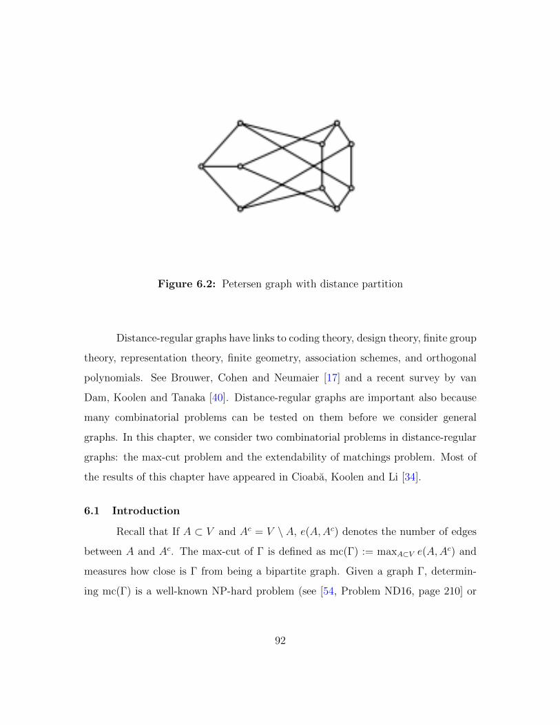
Figure 6.2: Petersen graph with distance partition

Distance-regular graphs have links to coding theory, design theory, finite group

theory, representation theory, finite geometry, association schemes, and orthogonal

polynomials. See Brouwer, Cohen and Neumaier [17] and a recent survey by van

Dam, Koolen and Tanaka [40]. Distance-regular graphs are important also because

many combinatorial problems can be tested on them before we consider general

graphs. In this chapter, we consider two combinatorial problems in distance-regular

graphs: the max-cut problem and the extendability of matchings problem. Most of

the results of this chapter have appeared in Cioaba, Koolen and Li [34].

6.1 Introduction

Recall that If A ⊂ V and Ac = V \ A, e(A,Ac) denotes the number of edges

between A and Ac. The max-cut of Γ is defined as mc(Γ) := maxA⊂V e(A,Ac) and

measures how close is Γ from being a bipartite graph. Given a graph Γ, determin-

ing mc(Γ) is a well-known NP-hard problem (see [54, Problem ND16, page 210] or

92

[69]) and designing efficient algorithms to approximate mc(Γ) has attracted a lot of

attention [4, 42, 43, 44, 57, 86, 99].

In Section 6.2, we obtain a simple upper bound for the max-cut of certain

regular graphs in terms of their odd girth (the shortest length of an odd cycle). In

Section 2, we prove that if Γ is a non-bipartite distance-regular graph with odd girth

g, then mc(Γ) ≤ e(1− 1g), where e := |E|. As a consequence of this result, we show

that if Γ is a non-bipartite distance-regular graph with odd girth g and independence

number α(Γ), then α(Γ) ≤ v2(1 − 1

g). We show that these bounds are incomparable

with some spectral bounds of Mohar and Poljak [86] for the max-cut and of Hoffman

[19, Theorem 3.5.2] for the independence number.

In Section 6.3, we generalize results in Chapter 5 and study the extendability

of distance-regular graphs with diameter D ≥ 3. Brouwer and Haemers [18] proved

that distance-regular graphs are k-edge-connected. Plesnık ([89] or [79, Chapter 7])

showed that if Γ is a k-regular (k − 1)-edge-connected graph with an even number

of vertices, then the graph obtained by removing any k − 1 edges of Γ contains a

perfect matching. Thus, every distance-regular graph is 1-extendable. We improve

this result and we show that all distance-regular graphs with diameter D ≥ 3 are

2-extendable. Let λ be the number of common neighbors of two adjacent vertices

and µ be the number of common neighbors of two vertices in distance 2. We also

show that distance-regular graphs of valency k ≥ 3 with λ ≥ 1 are bk+1− kλ+1

2c-

extendable (when µ = 1), b12dk+2

2ec-extendable (when µ = 2), dk−3

3e-extendable

(when 3 ≤ µ ≤ k/2), bk/3c-extendable (when µ > k/2) and bk+12c-extendable (when

the graph is bipartite).

6.2 Max-cut of Distance Regular Graphs

The following theorem is the main result of this section.

93

Theorem 6.2.1. Assume that Γ is a non-bipartite graph with odd girth g. If every

edge of Γ is contained in a constant number of cycles of length g, then

mc(Γ) ≤ e

(1− 1

g

). (6.1)

Proof. Let γ be the number of cycles of length g containing an edge e0. Let C be

the set of cycles of length g. Double count {(e0, C) | e0 ∈ E(Γ), C ∈ C and e0 is an

edge of C}. We have eγ = |C|g. Thus, |C| = eγg

. Let A be any subset of V and T be

all the edges in the graphs with both end points in A or both end points in Ac. If

we delete T , we will obtain a bipartite graph. Assume that we delete the edges in

T one by one. Every time we delete an edge in T , we destroy at most γ cycles in C.

And deleting T will destroy all the cycles of length g. We must have |T |γ ≥ |C|. As

a result, |T | ≥ eg

and e(A,Ac) = e− |T | ≤ e(1− 1g). As A is arbitrary, the theorem

follows.

Our theorem can be applied to the family of m-walk regular graphs with

m ≥ 1. This family of graphs contains the distance-regular graphs. A connected

graph Γ is m-walk-regular if the number of walks of length l between any pair of

vertices only depends on the distance between them, provided that this distance

does not exceed m. The family of m-walk-regular graphs was first introduced by

Dalfo, Fiol, and Garriga [39, 50].

Note that the upper bound of Theorem 6.2.1 is tight as shown for example

by the blow up of an odd cycle Cg. Consider the odd cycle Cg. If we replace each

vertex i of Cg by a coclique Ai (1 ≤ i ≤ g) of size m and add all the possible edges

between Ai and Aj whenever i and j are adjacent in Cg, then we will obtain a graph

with gm vertices and gm2 edges. The odd girth of this graph is g, each edge of the

graph is contained in the same number of cycles of length g and there is a cut of size

e(

1− 1g

)= (g − 1)m2.

94

Mohar and Poljak [86] obtained an upper bound for the max-cut in terms of

the Laplacian eigenvalues (see also [4, 42, 43, 44]). Translated to regular graphs,

their result implies the following inequality:

mc(Γ) ≤ e

2

(1− λv

k

). (6.2)

Note that the inequalities (6.1) and (6.2) are incomparable. This fact can be seen

by considering the complete graph and the odd cycle, but we give other examples of

distance-regular graphs later in this section.

The Hamming graph H(D, q) is the graph whose vertices are all the words

of length D over an alphabet of size q with two words being adjacent if and only

their Hamming distance is 1. The graph H(D, q) is distance-regular of diameter D,

has eigenvalues (q − 1)D − qi for 0 ≤ i ≤ D and is bipartite when q = 2 [19, page

174]. When q ≥ 3, inequality (6.1) always gives an upper bound 2e3

. The upper

bound from inequality (6.2) is e2(1 + 1

q−1). When q = 3, (6.1) is better. When q ≥ 5,

inequality (6.2) is better. When q = 4, both inequalities give the same upper bound.

The Johnson graph J(n,m) is the graph whose vertices are the m-subsets of a

set of size n with two m-subsets being adjacent if and only if they have m−1 elements

in common. The graph J(n,m) is distance-regular with diameter D = min(m,n−m),

eigenvalues (m − i)(n − m − i) − i, where 0 ≤ i ≤ D [19, page 175]. Inequality

(6.1) always gives an upper bound 2e3

. Inequality (6.2) is e2(1 + D

m(n−m)). When

max(m,n −m) ≥ 4, (6.2) is better. In other cases (m ∈ {2, 3}, n −m ∈ {1, 2, 3}),

(6.1) is better.

In the following examples, we compare (6.1) and (6.2) for other distance-

regular graph with larger odd girth.

1. The Dodecahedral graph [17, page 417] is a 3-regular graph of order 20 and

95

size 30. It has λv = −√

5 and g = 5. Inequality (6.1) gives mc(Γ) ≤ 24 and

inequality (6.2) gives mc(Γ) ≤ 26.

2. The Coxeter graph [17, page 419] is a 3-regular graph of order 28 and size 42.

It has λv = −√

2 − 1 ≈ −2.414 and g = 7. Inequality (6.1) gives mc(Γ) ≤ 36

and inequality (6.2) gives mc(Γ) ≤ 37.

3. The Biggs-Smith graph [17, page 414] is a 3-regular graph of order 102 and size

153. It has λv ≈ −2.532 and g = 9. Inequality (6.1) gives mc(Γ) ≤ 136 and

inequality (6.2) gives mc(Γ) ≤ 141.

4. The Wells graph [17, page 421] is a 5-regular graph of order 32 and size 80. It

has λv = −3 and g = 5. Inequality (6.1) gives mc(Γ) ≤ 64 and inequality (6.2)

gives mc(Γ) ≤ 64.

5. The Hoffman-Singleton graph [17, page 391] is a 7-regular graph of order 50

and size 175. It has θv = −3 and g = 5. Inequality (6.1) gives mc(Γ) ≤ 140

and inequality (6.2) gives mc(Γ) ≤ 125.

6. The Ivanov-Ivanov-Faradjev graph [17, page 414] is a 7-regular graph of order

990 and size 3465. It has θv = −4 and g = 5. Inequality (6.1) gives mc(Γ) ≤

2772 and inequality (6.2) gives mc(Γ) ≤ 2722.

7. The Odd graph Om+1 [17, page 259-260] is the graph whose vertices are the

m-subsets of a set with 2m + 1 elements, where two m-subsets are adjacent

if and only if they are disjoint. Note that O3 is Petersen graph. The graph

Om+1 is a distance-regular graph of valency m + 1, order v =(

2m+1m

)and size

e = m+12

(2m+1m

). It has θv = −m and g = 2m + 1. Inequality (6.1) gives

mc(Γ) ≤ e(1− 12m+1

) and inequality (6.2) gives mc(Γ) ≤ e(1− 12m+2

).

96

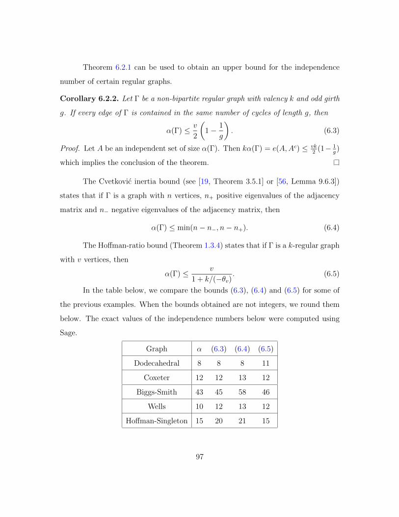
Theorem 6.2.1 can be used to obtain an upper bound for the independence

number of certain regular graphs.

Corollary 6.2.2. Let Γ be a non-bipartite regular graph with valency k and odd girth

g. If every edge of Γ is contained in the same number of cycles of length g, then

α(Γ) ≤ v

2

(1− 1

g

). (6.3)

Proof. Let A be an independent set of size α(Γ). Then kα(Γ) = e(A,Ac) ≤ vk2

(1− 1g)

which implies the conclusion of the theorem.

The Cvetkovic inertia bound (see [19, Theorem 3.5.1] or [56, Lemma 9.6.3])

states that if Γ is a graph with n vertices, n+ positive eigenvalues of the adjacency

matrix and n− negative eigenvalues of the adjacency matrix, then

α(Γ) ≤ min(n− n−, n− n+). (6.4)

The Hoffman-ratio bound (Theorem 1.3.4) states that if Γ is a k-regular graph

with v vertices, then

α(Γ) ≤ v

1 + k/(−θv). (6.5)

In the table below, we compare the bounds (6.3), (6.4) and (6.5) for some of

the previous examples. When the bounds obtained are not integers, we round them

below. The exact values of the independence numbers below were computed using

Sage.

Graph α (6.3) (6.4) (6.5)

Dodecahedral 8 8 8 11

Coxeter 12 12 13 12

Biggs-Smith 43 45 58 46

Wells 10 12 13 12

Hoffman-Singleton 15 20 21 15

97

For the Hamming graph H(D, q) with D = 2 and q ≥ 3, (6.3) is better than

(6.5). For the Hamming graph H(D, q) with D ≥ 3 and q ≥ 3, (6.5) is better. For

the Odd graph Om+1, the inequalities (6.3) and (6.5) give the same bound equals the

independence number of Om+1.

6.3 Extendability of Matchings in Distance-regular Graphs

In this section, we will focus on the extendability of distance-regular graphs.

A set of edges M of a graph Γ is a matching if no two edges of M share a vertex.

A matching M is perfect if every vertex is incident with exactly one edge of M .

A graph Γ of even order v is called t-extendable if it contains at least one perfect

matching, t < v/2 and any matching of size t is contained in some perfect matching.

In Subsection 6.3.1, we describe the main tools which will be used in our proofs.

In Subsection 6.3.2, we give various lower bounds for the extendability of distance-

regular graphs. In Subsection 6.3.3, we show that all distance-regular graphs with

diameter D ≥ 3 are 2-extendable.

6.3.1 Main tools

Theorem 6.3.1 (Brouwer and Haemers [18]). Let Γ be a distance-regular graph of

valency k. Then Γ is k-edge-connected. Moreover, if k > 2, then the only discon-

necting set of k edges are the set of k edges on a single vertex.

Theorem 6.3.2 (Brouwer and Koolen [21]). Let Γ be a distance-regular graph of

valency k. Then Γ is k-connected. Moreover, if k > 2, then the only disconnecting

sets of k vertices are the set of the neighbors of some vertex.

Lemma 6.3.3. Let Γ be a distance-regular graph with k ≥ 4. If A ⊂ V with

3 ≤ |A| ≤ k − 1, then e(A,Ac) ≥ 3k − 6.

98

Proof. If |A| ≤ k−2, then each vertex in A has at least k− (|A|−1) neighbors in Ac

and consequently e(A,Ac) ≥ |A|(k−|A|+1) ≥ 3(k−2). Let A ⊂ V with |A| = k−1.

If |N1(x)∩A| ≤ k− 3 for any x ∈ A, then e(A,Ac) ≥ 3(k− 1). Otherwise, let x ∈ A

such that |N1(x) ∩ A| = k − 2. Denote N1(x) ∩ Ac = {y, z}. At least λ− 1 of the λ

common neighbors of x and y are contained inA. Therefore, y has at least λ neighbors

in A. A similar statement holds for z. Thus, e(A,N1(x) ∩Ac) ≥ 2λ = 2(k − b1 − 1).

Also, e(N1(x) ∩ A,N2(x)) ≥ (k − 2)b1 so e(A,Ac) ≥ (k − 2)b1 + 2(k − b1 − 1) =

3k − 6 + (k − 4)(b1 − 1) ≥ 3k − 6.

We give the following characterization of bipartite non t-extendable graphs

that might be of independent interest.

Lemma 6.3.4. Let Γ be a bipartite graph with color classes X and Y , where |X| =

|Y | = m. The graph Γ is not t-extendable if and only if Γ has an independent set I

of size at least m− t+ 1, such that I 6⊂ X and I 6⊂ Y .

Proof. Assume that Γ is not t-extendable. Lemma 5.2.3 implies that there is a

vertex disconnecting set S such that the subgraph induced by S contains at least t

independent edges and o(Γ−S) ≥ |S| − 2t+ 2. Let S be such a disconnecting set of

maximum size. Our key observation is that Γ − S does not have non-singleton odd

components. Indeed, note that any non-singleton odd component of Γ − S induces

a bipartite graph with color classes A and B. Since |A| + |B| is odd, we get that

|A| 6= |B| and assume that |A| > |B|. If S ′ = S∪B, then S ′ is a vertex disconnecting

set with |S ′| > |S| and o(Γ− S ′) ≥ |S ′| − 2t+ 2, contradicting to the maximality of

|S|. By a similar argument, Γ− S contains no even components. Let I = V (Γ) \ S.

Then I is an independent set of size at least m − t + 1 since |I| + |S| = 2m and

|I| ≥ |S| − 2t + 2. Assume that I ⊂ X. Then S induces a bipartite graph with one

99

partite set of size at most t− 1. This makes it impossible for the subgraph induced

by S to contain t independent edges. The converse implication is immediate.

Note that the study of such independent sets in regular bipartite graphs has

been done by other authors in different contexts (see [41] for example).

Lemma 6.3.5 (Brouwer and Haemers [18]). Let Γ be a distance-regular graph and

T be a disconnecting set of edges of Γ, and let A be the vertex set of a component

of Γ minus T . Fix a vertex a ∈ A and let ti be the number of edges in T that join

Ni−1(a) and Ni(a). Then |A ∩Ni(a)| ≥ (1−∑i

j=1tjcjkj

)ki, so that

|A| ≥ v −∑i

ticiki

(ki + · · ·+ kD).

Further more, when T is a disconnecting set of edges none of which is incident with

a,

|A| > v

(1− |T |

µk2

).

Lemma 6.3.6. Let Γ be a distance-regular graph with λ ≥ 1. If A is an independent

set of Γ, then |N(T )| ≥ 2|T |.

Proof. The same as Lemma 5.2.6.

Lemma 6.3.7. Let Γ be a distance-regular graph with valency k ≥ 3, λ ≥ 1 and

µ ≤ k/2. If A is an independent set of Γ, then |N(A)| ≥ k + |A| − 1.

Proof. The same as Lemma 5.2.8.

A distance-regular graph with intersection array {k, µ, 1; 1, µ, k} is called a

Taylor graph.

Lemma 6.3.8. Let Γ be a non-bipartite distance-regular graph with D ≥ 3. If

k < 2µ, then Γ is a Taylor graph.

100

Proof. First we show that D ≥ 4 implies k ≥ 2µ; this is known (see [17, Theorem

1.9.3]), but we include a short proof here for the sake of completeness. If D ≥ 4,

then let x and y be two vertices of Γ at distance 4. If z ∈ N2(x) ∩ N2(y), then z

has µ neighbors in Γ(x) ∩ Γ(z) and µ neighbors in Γ(y) ∩ Γ(z) ⊂ N3(x). Therefore,

k ≥ 2µ, contradicting to the condition that k < 2µ.

Thus, D = 3. Let x ∈ V (Γ). We just need to prove that |N3(x)| = 1. This

implies k2 = c3 = k, and that Γ has intersection array {k, µ, 1; 1, µ, k}. Suppose that

|N3(x)| > 1. Note that a2 > 0 or a3 > 0. Otherwise, Γ being not bipartite and a2 =

a3 = 0 imply that a1 > 0. Let z ∈ N3(x). There is at least one triangle containing z

and any such triangle is contained in N≥2(x) contradicting a2 = a3 = 0. Also, if every

vertex in N2(x) is adjacent to every vertex in N3(x), then k2 = c3. Since k2 ≥ k ≥ c3,

this implies µ = c2 = k, impossible. Hence, there exists y ∈ N2(x), z ∈ N3(x), such

that y 6∼ z. Without loss of generality, we may assume that y and z are at distance

2. By Lemma 5.2.5, N≥2(x) is connected. As y has µ neighbors in Γ(x) ∩ Γ(y) and

µ neighbors in Γ(y) ∩ Γ(z) ⊂ N2(x) ∪N3(x), we have k ≥ 2µ, contradiction.

6.3.2 Lower bounds for the extendability of distance-regular graphs

In this subsection, we give some sufficient conditions, in term of k, λ and µ,

for a distance-regular graph to be t-extendable, where t ≥ 1.

Theorem 6.3.9. If Γ is a distance-regular graph with even order and λ ≥ 1, then Γ

is b12dk+2

2ec-extendable.

Proof. The graph Γ is K1,bk/2c+1-free because λ ≥ 1. Let t = b12dk+2

2ec and n =

bk/2c+ 1. Then k ≥ 2t+ n− 2. The result follows from Lemma 6.3.2 and Theorem

5.3.3.

We improve the previous result when µ = 1.

101

Theorem 6.3.10. If Γ be a distance-regular graph with even order, λ ≥ 1 and µ = 1,

then Γ is

⌊k+1− k

λ+1

2

⌋-extendable.

Proof. The condition µ = 1 implies that Γ1(x) is a disjoint union of cliques on λ+ 1

vertices. Hence, λ + 1 divides k and Γ is K1, kλ+1

+1-free. Let t =

⌊k+1− k

λ+1

2

⌋and

n = kλ+1

+ 1. Then 2t + n − 2 ≤ k. The conclusion follows from Lemma 6.3.2 and

Theorem 5.3.3.

The following theorem is an improvement of Theorem 6.3.9 when 3 ≤ µ ≤ k/2.

Theorem 6.3.11. Let Γ be a distance-regular graph with even order, and D ≥ 3. If

λ ≥ 1 and 3 ≤ µ ≤ k/2, then Γ is t-extendable, where t =⌈

(k−3)(k−1)3k−6

⌉.

Proof. If Γ is not t-extendable, by Lemma 5.2.3, there is a vertex set S with s

vertices such that the subgraph induced by S contains t independent edges, and

o(Γ− S) ≥ s− 2t + 2. Let S be a disconnecting set with minimum cardinality and

o(Γ− S) ≥ s− 2t + 2. Note that such S may not contain t independent edges. Let

O1, O2, . . . , Or be all the odd components of Γ − S, with r ≥ s − 2t + 2. Let a ≥ 0

denote the number singleton components among O1, . . . , Or.

We claim that e(A, S) ≥ 3k− 6 for any non-singleton component A of Γ− S.

Let A be a non-singleton odd component of Γ − S and B = (A ∪ N(A))c.

If |A| ≤ k − 1, the claim follows from Lemma 6.3.3. Assume that |A| ≥ k. Let

S ′ := {s ∈ N(A) | N(s) ⊆ A ∪ N(A)}. Then |S ′| ≤ 1. Otherwise, assume that

x 6= y ∈ S ′. Define S0 = S \ {x, y} and A0 = A ∪ {x, y}. Then S0 is a disconnecting

set with o(Γ − S ′) = o(Γ − S) ≥ |S| − 2t + 2 > |S ′| − 2t + 2, contradicting the

minimality of |S|.

If we let A′ := {a ∈ A | d(a, b) = 2 for some b ∈ B}, then e(A, S) ≥ µ|A′|.

If |A′| ≥ k − 2, we get e(A, S) ≥ µ|A′| ≥ 3(k − 2) and we are done. Otherwise, if

102

|A′| < k− 2, then the set A′ ∪ S ′ is a disconnecting set with less than k− 1 vertices,

contradicting Lemma 6.3.2. This finishes our proof of the claim.

Counting the number of edges between S and O1 ∪ · · · ∪ Or, we obtain the

following

ks ≥ e(S,O1∪ · · ·∪Or) ≥ ak+ (r−a)(3k−6) ≥ ak+ (s−2t+ 2−a)(3k−6). (6.6)

This inequality is equivalent to

t ≥ (k − 3)(s− a) + 3k − 6

3k − 6(6.7)

and since s− a ≥ k − 1 (Lemma 6.3.7), we obtain that

t ≥ (k − 3)(k − 1)

3k − 6+ 1. (6.8)

This is a contradiction with t =⌈

(k−3)(k−1)3k−6

⌉.

Theorem 6.3.12. Let Γ be a non-bipartite distance-regular graph with D ≥ 3 and

µ > k/2, then Γ is t-extendable, where t = bk/3c when λ ≥ 1 and t = k − 1 when

λ = 0.

Proof. Lemma 6.3.8 implies that Γ is a Taylor graph with intersection array

{k, µ, 1; 1, µ, k}. If λ = 0, then µ = k − 1 and Γ is obtained by deleting a perfect

matching from K(k+1)×(k+1) (see [17, Corollary 1.5.4]). It is straightforward to show

that Γ is (k − 1)-extendable.

Assume that λ ≥ 1. It is known that for any x ∈ V (Γ), Γ1(x) is a strongly

regular graph with parameters(k, λ, 3λ−k−1

2, λ

2

)(see [17, Section 1.5]). If 3λ−k−1

2≥ 1,

then Lemma 6.3.6 implies that α(Γ1(x)) ≤ k/3. If Γ is not t-extendable, then there

is a vertex disconnecting set S containing t independent edges, such that Γ− S has

at least s− 2t + 2 ≥ k − 2t + 2 ≥ 3 odd components. Picking one vertex from each

103

odd component yields an independent set I in Γ. If two vertices of this independent

set were at distance 3, then the neighborhood of these two vertices will be formed by

the remaining 2k vertices of the graph and therefore, Γ−S would have only two odd

components, contradiction. Thus, assume that any two vertices of this independent

set are at distance 2 to each other. Pick a vertex x in this independent set. Any

subset of k − 2t+ 1 vertices of I \ {x} will be an independent set in Γ1(y), where y

is the antipodal vertex to x. Thus, k − 2t + 1 ≤ k/3, contradiction with t = bk/3c.

If 3λ−k−12

= 0, then Γ1(x) has parameters (3λ − 1, λ, 0, λ/2). If λ = 2, Γ1(x) is C5

which implies that k = 5 and µ = 2, contradiction with k/2 < µ. If λ ≥ 4, then

Γ1(x) must have integer eigenvalues implying that x2 + λ2x− λ

2= 0 has integer roots.

However, (λ/2)2 + 2λ is not a perfect square, contradiction.

In the end of this subsection, we will show that bipartite distance-regular

graphs have high extendability.

Theorem 6.3.13. If Γ is a bipartite distance-regular graph with valency k, then Γ

is t-extendable, where t = bk+12c.

Proof. Let X and Y be the color classes of Γ, where |X| = |Y | = m. Assume that Γ is

not t-extendable. By Lemma 6.3.4, Γ has an independent set I of size at leastm−t+1,

such that I 6⊂ X and I 6⊂ Y . Let A = I ∩X, B = I ∩ Y , C = X \A, D = Y \B. If

|A| = a, then |B| ≥ m− a− t+ 1, |C| = m− a and |D| ≤ a+ t− 1. As there are ak

edges between A and D, and (a + t − 1)k ≥ |D|k = e(D,X) = e(A,D) + e(C,D),

there are at most (t− 1)k edges between C and D. This implies that Γ has an edge

cut of size at most (t − 1)k, which disconnects Γ into two vertex sets B ∪ C and

104

A ∪D. Without loss of generality, assume that |A ∪D| ≤ m. By the second part of

Lemma 6.3.5, we have

|A ∪D| > v

(1− e(A ∪D,B ∪ C)

µk2

)≥ 2m

(1− (t− 1)k

(k − 1)k

)≥ 2m(1− 1/2) = m,

contradiction with |A ∪D| ≤ m.

6.3.3 The 2-extendability of distance-regular graphs of valency k ≥ 3

Lou and Zhu [81] proved that any strongly regular graph of even order is 2-

extendable with the exception of the complete tripartite graphK2,2,2 and the Petersen

graph. Cioaba and Li [36] showed that any strongly regular graph of even order and

valency k ≥ 5 is 3-extendable with the exception of the complete 4-partite graph

K2,2,2,2, the complement of the Petersen graph and the Shrikhande graph (see [18,

page 123] for a description of this graph).

In this subsection, we prove that any distance-regular graph of diameter D ≥ 3

is 2-extendable. By Theorem 6.3.9, any distance-regular graph with λ ≥ 1 and k ≥ 5

is 2-extendable. Note also that any distance-regular graph of even order having

valency k ≤ 4 and diameter D ≥ 3 must have λ = 0 (see [13, 20]). Theorem 6.3.13

implies that any bipartite distance-regular graph of valency k ≥ 3 is 2-extendable.

Thus, we only need to settle the case of non-bipartite distance-regular graphs with

λ = 0. We will need the following lemma.

Lemma 6.3.14. If Γ is a non-bipartite distance-regular graph with valency k ≥ 5

and λ = 0, then α(Γ) < v/2− 1.

Proof. If g is the odd girth of Γ, then v > 2g and Corollary 6.2.2 implies that

α(Γ) ≤ v2(1− 1

g) < v/2− 1.

Theorem 6.3.15. If Γ is a non-bipartite distance-regular graph with even order,

valency k ≥ 3 and λ = 0, then Γ is 2-extendable.

105

Proof. We prove this result by contradiction and the outline of our proof is the

following. We assume that Γ is not 2-extendable. Lemma 5.2.3 implies that there

is a vertex disconnecting set S, such that the graph induced by S contains at least

2 independent edges and o(Γ − S) ≥ |S| − 2. Without loss of generality, we may

assume that S is such a disconnecting set with the maximum size. We then prove

that Γ− S does not have non-singleton components which implies that V (Γ)− S is

an independent set of size at least v/2− 1, contradiction to Lemma 6.3.14.

Assume k ≥ 5 first.

Note that any odd non-singleton component of Γ−S is not bipartite. Other-

wise, assume there is a bipartite odd component of Γ − S with color classes X and

Y such that |X| > |Y |. Let S ′ = S ∪ Y . Then |S ′| > |S| and o(Γ − S ′) ≥ |S ′| − 2,

contradiction with |S| being maximum. Also, Γ− S has no even components. Oth-

erwise, we can add one vertex of one such even component to S and creating a larger

disconnecting set and an extra odd component, contradicting again the maximality

of |S|. It is easy to see that Γ − S does not have any components with 3 vertices,

because Γ is triangle free and any component with 3 vertices must be a path, hence

bipartite.

Assume that A is an odd non-singleton component of Γ− S. If we can show

that e(A, S) ≥ 3k−3, then we obtain a contradiction by counting the edges between

S and Sc:

k|S| − 4 ≥ e(S, Sc) ≥ 3k − 3 + k(|S| − 3) = k|S| − 3, (6.9)

finishing our proof.

We now prove e(A, S) ≥ 3k−3 whenever A is a non-singleton odd component

of Γ− S.

If 5 ≤ |A| ≤ 2k−3, then as A has no triangle, Turan’s theorem implies that A

106

contains at most |A|2−14

edges. Thus, e(A, S) ≥ k|A|−2e(A) ≥ k|A|− |A|2−12≥ 3k−4.

The last equality is attained when A induces a bipartite graph Kk−1,k−2. This is

impossible as the graph induced by A is not bipartite. Hence, e(A, S) ≥ 3k − 3.

Let A be an odd component of Γ− S such that |A| ≥ 2k − 1. If every vertex

of A sends at least one edge to S, then we have two subcases: µ ≥ 2 and µ = 1.

If µ ≥ 2, then we can define S ′ := {s ∈ N(A) | N(s) ⊆ A∪N(A)}. If |S ′| ≥ 3,

then e(A, S)+2e(S) ≥ 3k+1. This is because e(A, S)+2e(S) =∑

x∈S |N(x)∩(A∪S)|.

As the graph induced by S contains at least 2 independent edges, the previous sum

contains at least 4 positive terms, and at least 3 of such terms are equal to k. On the

other hand, e(A, S)+(|S|−3)k ≤ e(S, Sc) = |S|k−2e(S). Thus, e(A, S)+2e(S) ≤ 3k,

contradiction. If |S ′| ≤ 2, then let B = (A ∪ N(A))c and A′ = {a ∈ A | ∃b ∈

B such that d(a, b) = 2}. Because A′ ∪ S ′ is a disconnecting set, Lemma 3.3.2

implies that |A′ ∪ S ′| ≥ k and therefore, |A′| ≥ k − 2. As each vertex in A′ sends at

least µ edges to S and µ ≥ 2, we get that e(A, S) ≥ 2k− 1 + (k− 2)(µ− 1) ≥ 3k− 3.

If µ = 1, then A contains no triangles or four-cycles. If |A| ≥ 3k − 3, then

e(A, S) ≥ 3k − 3, as every vertex of A sends at least one edge to S. If |A| ≤ 3k − 4,

then e(A) ≤ |A|√|A|−1

2since A contains no triangles or four-cycles (see [55, Theorem

2.2] or [76, Theorem 4.2]). Since also 2k − 1 ≤ |A| ≤ 3k − 4, we get that e(A, S) =

k|A| − 2e(A) ≥ |A|(k −√|A| − 1) ≥ (2k − 1)(k −

√3k − 5) ≥ 3k − 3.

The only case remaining is when |A| ≥ 2k − 1 and A has a vertex x having

no neighbors in S (such a vertex is called a deep point in [20]). Note that Ac always

has a deep point because every vertex in V (Γ) \ (A ∪ S) is a deep point of Ac. We

have two cases:

1. When k ≥ 6, we will show that e(A, S) ≥ 3k− 3. Otherwise, by Lemma 6.3.5,

|A| > v

(1− 3k − 4

µk2

)= v

(1− 3k − 4

k(k − 1)

)≥ v/2. (6.10)

107

The last inequality is true since k ≥ 6. As Ac always has a deep point, by

Lemma 6.3.5 again, we get that |Ac| > v/2, contradiction.

2. When k = 5, we do not have inequality (6.10) so we need a different proof. If

µ ≥ 3, by Lemma 6.3.8, Γ must be a Taylor graph. As λ = 0, by Theorem

6.3.12, Γ is 4-extendable. So, we must have 1 ≤ µ ≤ 2.

We first show that A is the only non-singleton component of Γ−S. Assume that

there are at least two non-singleton components in Γ−S. Let B be another non-

singleton component of Γ−S. Then B has a deep point, by previous arguments.

If e(A, S) ≥ 2k − 1 and e(B, S) ≥ 2k − 1, then k|S| − 4 ≥ e(S, Sc) ≥ 2(2k −

1) + (|S| − 4)k = k|S| − 2, contradiction. Without loss of generality, assume

that e(A, S) ≤ 2k − 2. By Lemma 6.3.5, |A| > v(

1− 2k−2µk2

)= v

(1− 2

k

)= 3v

5.

On the other hand, Lemma 6.3.5 also implies that |Ac| > 3v5

, contradiction.

Thus, A is the only non-singleton components in Γ − S. Recall that |A| ≥

2k − 1 and A has a deep point x. If e(A, S) ≤ 3k − 5, by Lemma 6.3.5,

|A| > v(

1− 3k−5µk2

)= v

(1− 10

20

)≥ v/2. Lemma 6.3.5 also implies that |Ac| >

v/2, contradiction. If e(A, S) = 3k − 4 = 11, by counting the edges between

S and Sc, we know that S contains exactly two independent edges. Also,

o(Γ − S) = |S| − 2. Let T be the set of singleton components of Γ − S. We

have |T | = |S| − 3. By Theorem 6.3.2, |S| ≥ k + 1 = 6 and |T | ≥ 3.

Now, we have two subcases:

(i) Assume that µ = 2. Let W = {a ∈ A | ∃s ∈ S, a ∼ s}. Note that W ⊂ A

and W is a disconnecting set of Γ. By Theorem 6.3.2, |W | ≥ 5 and the

only disconnecting sets of 5 vertices are the neighbors of some vertex.

If |W | = 5, then we have W = N(x) for some vertex x. By Lemma

108

5.2.5, the subgraph induced by the vertices at distance 2 or more from x

is connected. In other words, W disconnects Γ into two components, x

and V \ (W ∪ {x}). Since |Ac| > 1, we must have Ac = V \ (W ∪ {x})

and A \W = {x}. Hence, |A| = 6, contradicting to that |A| is odd. So,

|W | ≥ 6.

We claim that for any x ∈ W , there exists t ∈ T such d(x, t) = 2. As

µ = 2, each vertex in W has at least 2 neighbors in S and e(A, S) ≥ 12,

which is also a contradiction.

Assume that the claim above is not true. Then there is s ∈ S such

that N(s) ⊂ A ∪ S. Since the graph induced by S contains exactly

two independent edges, s has at most one neighbor in S and at least

four neighbors in A. If we let A′ = A ∪ {s} and S ′ = S \ {s}, then

e(A′, S ′) ≤ 8. By Lemma 6.3.5, |A′| > v(

1− 8µk2

)= v

(1− 8

20

)= 3v

5. On

the other hand, Lemma 6.3.5 also implies that |(A′)c| > 3v5

, contradiction.

(ii) Assume that µ = 1. We will first prove that a2 ≤ 1. If for every s ∈

S, |N(s) ∩ T | ≤ 2, by counting the edges between S and T , we have

5|T | = e(S, T ) ≤ 2|S|. On the other hand, |T | = |S| − 3 ≥ 52|T | − 3,

thus |T | ≤ 2, contradicting to |T | ≥ 3. Hence, there exists s ∈ S such

that |N(s) ∩ T | ≥ 3. Let x, y, z ∈ N(s) ∩ T . As µ = 1, N(x) ∩ N(y) =

N(y)∩N(z) = N(x)∩N(z) = {s}. Let U = (N(x)∪N(y)∪N(z)) \ {s}.

It is easy to check that U ⊂ N2(s), |U | = 12, |N2(s)| = 20, and Γ2(s)

is a2-regular. Since there are at most two edges inside U , 12a2 − 4 ≤

e(U,N2(s) \ U) ≤ 8a2 and thus a2 ≤ 1.

Note that µ = 1 and a2 ≤ 1 imply that b2 ≥ 3. If there exists r ∈ S, such

that N(r) ⊂ T , then d(r, A) ≥ 3. By Lemma 6.3.5, |Ac| > v(

1− 3k−4k2b2

)≥

109

v(1− 11

60

)= 49v

60. On the other hand, Lemma 6.3.5 also implies that

|A| >(

1− 3k−4µk2

)= v

(1− 3k−4

k(k−1)

)= 9v

20, contradiction. Thus, for all

r ∈ S, we have N(r) 6⊂ T . Consider the edges between T and S. We have

5|T | = e(T, S) ≤ 4|S| and therefore, |T | ≥ |S| − 3 ≥ 5|T |/4 − 3. Thus,

|T | ≤ 12, |S| ≤ 15, 27 ≥ |Ac| > 9v/20 and v < 60. Note that there is no

distance-regular graph with v < 60, k = 5, λ = 0, µ = 1 and a2 ≤ 1, see

the table [13].

This finishes the proof of the case k ≥ 5.

When k = 4, all the distance-regular graphs with even order are bipartite [20]

so we are done by Theorem 6.3.13.

When k = 3, there are 3 non-bipartite triangle-free distance-regular graphs

with even order (see [9] or [17, Chapter 7]): the Coxeter graph (intersection array

{3, 2, 2, 1; 1, 1, 1, 2}), the Dodecahedral graph (intersection array {3, 2, 1, 1, 1; 1, 1, 1, 2, 3})

and the Biggs-Smith graph (intersection array {3, 2, 2, 2, 1, 1, 1, ; 1, 1, 1, 1, 1, 1, 3}).

We will show that each one of them is 2-extendable.

Let Γ be the Coxeter graph. Then Γ has 28 vertices, girth 7 and independence

number 12 (see [8] for example). If Γ is not 2-extendable, there is a disconnecting

set S of maximum size, such that the graph induced by S contains 2 independent

edges and o(Γ − S) ≥ |S| − 2. As |S| ≥ 4, we have o(Γ − S) ≥ 2. Assume that

Γ − S contains a non-singleton component A. As |Ac| ≥ |S| + 1 ≥ 5, we have

3 ≤ |A| ≤ v − |Ac| ≤ 23. If 3 ≤ |A| ≤ 5, the graph induced by A is bipartite as the

girth of Γ is 7. As in the case k ≥ 5, we can construct a larger disconnecting set

contradicting the maximality of S. If |Ac| = 5, then Ac induces a bipartite graph and

e(A,Ac) = 3|Ac| − 2e(Ac) ≥ 7. If 7 ≤ |A| ≤ 21 and e(A,Ac) ≥ |A|(28−|A|)28

≥ 7×2128

> 5

(Theorem 1.4.1). In the above two cases, we have e(A, S) ≥ 3k − 3 = 6. Similar to

110

(6.9), this will lead to a contradiction. Thus, Γ− S has only singleton components.

Thus, α(Γ) ≥ o(Γ−S) ≥ max(28− |S|, |S| − 2) ≥ 13, contradiction with α(Γ) = 12.

Let Γ be the Dodecahedral graph. Then Γ has 20 vertices, girth 5 and inde-

pendence number 8 (see [56, pp.116] for example). If Γ is not 2-extendable, there is

a disconnecting set S of maximum size, such that the graph induced by S contains

2 independent edges and o(Γ− S) ≥ |S| − 2. As |S| ≥ 4, we have o(Γ− S) ≥ 2. As-

sume that Γ − S contains a non-singleton component A. As |Ac| ≥ |S| + 1 ≥ 5,

we have 3 ≤ |A| ≤ 15. We will prove that |A| 6= 3, 5, 7, 9 and |Ac| 6= 5, 7, 9.

By maximality of |S|, the graph induced by A is not bipartite. So, |A| 6= 3. If

|A| = 7, then the graph induced by A contains at most one cycle. Thus, e(A) ≤ 7

and e(A,Ac) = 3|A| − 2e(A) ≥ 7. If |A| = 9, then the graph induced by A con-

tains at most two cycles. Thus, e(A) ≤ 10 and e(A,Ac) = 3|A| − 2e(A) ≥ 7.

In either case, we will obtain a contradiction by inequality (6.9). Using the same

argument, we can show that |Ac| 6= 7, 9. If |Ac| = 5, then Ac induces either a bi-

partite graph or a pentagon. If Ac induces a bipartite graph, then e(Ac) ≤ 4 and

e(A,Ac) = 3|Ac| − 2e(Ac) ≥ 7, contradiction by inequality (6.9). If Ac induces a

pentagon, then every vertex in Ac is connected to A, and Γ − S has only one odd

component A, which is because S ⊂ Ac. The last case is |A| = 5. Since Γ − S has

no bipartite component, A must induce a pentagon. Consider the edges between S

and Sc, we have 3|S| − 4 ≥ e(S, Sc) ≥ 5 + 3(o(Γ−S)− 1). Thus, |S| − 2 ≥ o(Γ−S).

Combining with o(Γ−S) ≥ |S| − 2, we have o(Γ−S) = |S| − 2 and equality implies

that S contains exactly 2 edges and Γ−S contains exactly one non-singleton compo-

nent. Since |S|+ |A|+ o(Γ−S)−1 = 20, we have |S| = 9 and o(Γ−S) = 7. Assume

that x, y ∈ A such that x and y are not adjacent in A. Let U = S ∪ {x} ∪ {y}.

Then the graph induced by U contains exactly 4 edges and the graph induced by

U c contains exactly one edge. Hence, e(U,U c) = 25. However, by Theorem 6.2.1,

111

mc(Γ) ≤ e(

1− 1g

)= 24, contradiction. Thus, Γ−S has only singleton components.

Therefore, α(Γ) ≥ o(Γ−S) ≥ max(20−|S|, |S|−2) ≥ 9, contradiction with α(Γ) = 8.

Let Γ be the Biggs-Smith graph. Then Γ has girth 9 and 102 vertices. If

Γ is not 2-extendable, there is a disconnecting set S of maximum size, such that

the graph induced by S contains 2 independent edges and o(Γ − S) ≥ |S| − 2.

Assume that Γ − S contains a non-singleton component A. By similar argument

as the previous cases, we can assume that 5 ≤ |A| ≤ 97. When 5 ≤ |A| ≤ 7,

e(A) = |A| − 1 and e(A,Ac) = 3|A| − 2e(A) = |A| + 2 ≥ 7 . When 9 ≤ |A| ≤ 15,

e(A) ≤ |A| and e(A,Ac) = 3|A| − 2e(A) ≥ |A| ≥ 9. When 17 ≤ |A| ≤ 51, e(A,Ac) ≥(3−2.56155)|A|(102−|A|)

102≥ 6.21134 > 6 (by Theorem 1.4.1). If e(A, S) ≥ 3k − 3 = 6, we

will obtain a contradiction by inequality (6.9). Using the same argument, we can

obtain a contradiction when 5 ≤ |Ac| ≤ 51. Thus, all the components of Γ − S are

singletons. Therefore, α(Γ) ≥ o(Γ−S) ≥ max(102−|S|, |S|−2) ≥ 50, contradiction

with α(Γ) = 43 (see the table on page 5).

6.4 Remarks

Note that some of the bounds in this chapter can be improved if we have

a good lower bound for e(A,Ac) with k ≤ |A| ≤ v − k. We make the following

conjecture at the end of this chapter.

Conjecture 6.4.1. If Γ is a distance-regular graph of valency k, even order v and

diameter D ≥ 3, then the extendability of Γ is at least dk/2e − 1.

112

BIBLIOGRAPHY

[1] R.E.L. Aldred, D.A. Holton and D. Lou, n-extendability of symmetric graphs,J. Graph Theory 17 (1993), 253–261.

[2] R.E.L. Aldred and M.D. Plummer, On matching extensions with prescribedand proscribed edge sets. II, 16th British Combinatorial Conference (London,1997). Discrete Math. 197/198 (1999), 29–40.

[3] N. Alon and V.D. Milman, λ1 isoperimetric inequalities for graphs and super-concentrators, J. Comb. Theory B 38 (1985), 73-88.

[4] N. Alon and B. Sudakov, Bipartite subgraphs and the smallest eigenvalue,Combinatorics, Probability and Computing 9 (2000), 1–12.

[5] L. Babai, Spectra of Cayley graphs, J. Combin. Theory Ser. B 27 (1979),180–189.

[6] B. Bagchi, On strongly regular graphs with µ ≤ 2, Discrete Math. 306 (2006),no. 14, 1502–1504.

[7] C. Balbuena, A. Carmona, J. Fabrega and M.A. Fiol, Extraconnectivity ofgraphs with large minimum degree and girth, Discrete Math. 167/168 (1997),85–100.

[8] N.L. Biggs, Three remarkable graphs, Canad. J. Math. 25 (1973), 397–411.

[9] N.L. Biggs, A.G. Boshier and J. Shawe-Taylor, Cubic distance-regular graphs,J. London Math. Soc. (2), 33 (1986), 385–394.

[10] F. Boesch and R. Tindell, Circulants and their connectivities, J. Graph Theory8 (1994), 487–499

[11] B. Bollobas, Modern Graph Theory, Springer-Verlag New York Inc., 1998.

[12] J. A. Bondy and M. Simonovits, Cycles of even length in graphs, J. Combin.Theory Ser. B 16 (1974), 97–105.

113

[13] A. E. Brouwer, The uniqueness of the strongly regular graph on 77 points,Journal of Graph Theory 7 (1983), 455-461.

[14] A.E. Brouwer, Connectivity and spectrum of graphs, CWI Quarterly 9 (1996),37–40.

[15] A.E. Brouwer, Parameter sets for distance-regular graphs on at most 4096 ver-tices, list available at http:// www.win.tue.nl/∼aeb/drg/drgtables.html.

[16] A.E. Brouwer, Parameters of Strongly Regular Graphs, available online athttp://www.win.tue.nl/ aeb/graphs/srg/srgtab.html

[17] A.E. Brouwer, A. Cohen and A. Neumaier, Distance-Regular Graphs, Ergeb-nisse der Mathematik und ihrer Grenzgebiete, Springer-Verlag, 1989.

[18] A.E. Brouwer and W.H. Haemers, Eigenvalue and perfect matchings, LinearAlgebra and its Applications 395 (2005), 155-162

[19] A.E. Brouwer and W.H. Haemers, Spectra of Graphs, Springer Universitext.Springer, New York, 2012. xiv+250 pp.

[20] A.E. Brouwer and J.H. Koolen, The Distance-Regular Graphs of Valency Four,Journal of Algebraic Combinatorics 10 Issue 1 (1999), 5–24.

[21] A.E. Brouwer and J.H. Koolen, The vertex-connectivity of distance-regulargraphs, European J. Combin. 30 (2009), 668–673.

[22] A.E. Brouwer and J. van Lint, Strongly regular graphs and and partial geome-tries, in Enumeration and design (Waterloo, Ont., 1982), 85–122, AcademicPress, Toronto, ON, 1984.

[23] A.E. Brouwer and D.M. Mesner, The connectivity for strongly regular graphs,European J. Combin. 6 (1985), 215–216.

[24] A.E. Brouwer and A. Neumaier, A remark on partial linear spaces of girth 5with an application to strongly regular graphs, Combinatorica 8 (1988), no.1, 57–61.

[25] P.J. Cameron, Strongly regular graphs, in Topics in Algebraic Graph Theory(ed. L. W. Beineke and R. J. Wilson), Cambridge Univ. Press, Cambridge,2004 (ISBN 0521801974), pp. 203-221.

114

[26] P.J. Cameron, Random strongly regular graphs?, EuroComb’01 (Barcelona).Discrete Math. 273 (2003), no. 1–3, 103–114.

[27] P.J. Cameron and J. van Lint, Designs, Graphs, Codes and their Links, LondonMathematical Society Student Texts, 22, Cambridge, 1991. x+240 pp.

[28] X. Cao, M. Lu, D. Wan, L. Wang and Q. Wang, Linearized Wenger graphs,arXiv:1412.0179

[29] C. Chen, Matchings and matching extensions in graphs, Discrete Math. 186(1998), 95-103

[30] S.M. Cioaba, D.A. Gregory and W.H. Haemers, Matchings in regular graphsfrom eigenvalues, J. Combin. Theory Ser. B 99 (2009), 287–297.

[31] S.M. Cioaba, K. Kim and J.H. Koolen, On a conjecture of Brouwer involvingthe connectivity of strongly regular graphs, J. Combin. Theory Ser. A 119(2012), 904-922.

[32] S.M. Cioaba and J.H. Koolen, On the connectedness of the complement of aball in distance-regular graphs, Journal of Algebraic Combinatorics 38 (2013),191–195.

[33] S.M. Cioaba, J.H. Koolen and W. Li, Disconnecting strongly regular graphs,European J. Combin. 38 (2014), 1–11.

[34] S.M. Cioaba, J.H. Koolen and W. Li, Max-cut and extendability of matchingsin distance-regular graphs, in preparation.

[35] S.M. Cioaba, F. Lazebnik and W. Li, On the spectrum of Wenger graphs,Journal of Combinatorial Theory, Series B 107 (2014), 132-139.

[36] S.M. Cioaba and W. Li, The extendability of matchings in strongly regulargraphs, Electronic Journal of Combinatorics 21, Issue 2 (2014), P2.34

[37] S. D. Cohen, The values of a polynomial over a finite field, Glasgow Math. J.14 (1973), 205–208.

[38] K. Coolsaet, J. Degraer and T. Spence, The strongly regular (45, 12, 3, 3)graphs, Electronic J. Combin. 13 (2006), R32.

[39] C. Dalfo, M. A. Fiol and E. Garriga, On k-walk-regular graphs, The ElectronicJournal of Combinatorics 16 (2009), R47.

115

[40] E. van Dam, J.H. Koolen, H. Tanaka, Distance-regular graphs,http://arxiv.org/abs/1410.6294.

[41] S. de Winter, J. Schillewaert and J. Verstraete, Large incidence-free sets ingeometries, Electron. J. Combin. 19 (2012), Paper 24.

[42] C. Delorme and S. Poljak, Laplacian eigenvalues and the maximum cut prob-lem, Math. Programming 62 (1993), 557–574.

[43] C. Delorme and S. Poljak, Combinatorial properties and the complexity of amax-cut problem, European J. Combin. 14 (1993), 313–333.

[44] C. Delorme and S. Poljak, The performance of an eigenvalue bound on themax-cut in some classes of graphs, Discrete Math. 111 (1993), 145–156.

[45] Ph. Delsarte, J.-M. Goethals and J. J. Seidel, Spherical codes and designs,Geom. Dedicata 6 (1977), 363–388.

[46] P. Diaconis and M. Shahshahani, Generating a random permutation withrandom transpositions, Zeit. fur Wahrscheinlichkeitstheorie verw. Gebiete, 57(1981), 159-179. (p. 96)

[47] D.S. Dummit and R.M. Foote, Abstract Algebra, Wiley; 3rd edition , 2003

[48] L. Esperet, F. Kardos, A.D. King, D. Kral and S. Norine, Exponentially manyperfect matchings in cubic graphs, Adv. Math. 227 (2011), 1646–1664.

[49] N.C. Fiala and W.H. Haemers, 5-chromatic strongly regular graphs, DiscreteMath. 306 (2006), 3083–3096.

[50] M. A. Fiol and E. Garriga. Spectral and geometric properties of k-walk-regulargraph, Electron. Notes Discrete Math 29 (2007), 333–337.

[51] S. Friedland, Results and open problems in matchings in regular graphs, Elec-tron. J. Linear Algebra 24 (2012), 18–33.

[52] V. Futorny and V. Ustimenko, On small world semiplanes with generalizedSchubert cells, Acta Appl. Math. 98 (2007), 47–61.

[53] T. Gallai, Neuer Beweis eines Tutte’schen Satzes, Magyar Tud. Akad. Mat.Kut. Int. Kozl. 8 (1963), 135–139.

116

[54] M.R. Garey and D.S. Johnson, Computers and Intractability: A Guide to theTheory of NP-Completeness. A Series of Books in the Mathematical Sciences.San Francisco, Calif.: W. H. Freeman and Co. 1979, pp. x+338.

[55] D.K. Garnick, Y.H. Kwong and F. Lazebnik, Extremal Graphs without Three-Cycles or Four-Cycles, Journal of Graph Theory 17 (1993), 633–645.

[56] C. Godsil and G. Royle, Algebraic Graph Theory, Springer Graduate Texts inMathematics, 207. Springer-Verlag, New York, 2001. xx+439 pp.

[57] X. Goemans and D. Williamson, Improved approximation algorithms for maxi-mum cut and satisfiability problems using semidefinite programming, J. Assoc.Comput. Mach. 42 (1995), no. 6, 1115–1145.

[58] W.H.Haemers, Eigenvalue techniques in design and graph theory, Ph. D. The-sis, Technical University Eindhoven (1979).

[59] J.I. Hall, Classifying copolar spaces and graphs, Quart. J. Math. Oxford 33(1982), 421–449.

[60] Y.O. Hamidoune, A.S. Llado and O. Serra, An isoperimetric problem in Cayleygraphs, Theory Comput. Systems 32 (1999), 507–516.

[61] Y.O. Hamidoune, A.S. Llado, O. Serra and R. Tindell, On isoperimetric con-nectivity in vertex-transitive graphs, SIAM J. Discrete Math. 13 (2000), 139–144.

[62] A.J. Hoffman, R.R Singleton. On Moore Graphs with Diameters 2 and 3, IBMJournal of Research and Development 4 (1960), 497–504.

[63] R.A. Horn and C.R. Johnson, Matrix Analysis, Cambridge University Press,New York, 1985.

[64] S. Hoory, N. Linial, and A. Wigderson. Expander graphs and their applications.Bull. Amer. Math. Soc. 43 (4) (2006), 439–561.

[65] D. Holton and D. Lou, Matching extensions of strongly regular graphs, Aus-tralas. J. Combin. 6 (1992), 187–208.

[66] S. Hoory, N. Linial and A. Wigderson, Expanders and their applications, Bull.Amer. Math. Soc. 43 (2006), 439–561.

117

[67] K. Ireland and M. Rosen, A classical Introduction to Modern Number Theory,Springer, 2nd edition, 1998.

[68] I.M. Isaacs Algebra, American Mathematical Society, 2009

[69] R. Karp, Reducibility among combinatorial problems, Complexity of computercomputations (Proc. Sympos., IBM Thomas J. Watson Res. Center, YorktownHeights, N.Y., 1972), pp. 85–103. Plenum, New York, 1972.

[70] A. Knopfmacher and J. Knopfmacher, Counting polynomials with a given num-ber of zeros in a finite field, Linear and Multilinear Algebra 26 (1990), 287–292.

[71] F. Lazebnik and V. Ustimenko, New examples of graphs without small cyclesand of large size, European J. Combin. 14 (1993), 445–460.

[72] F. Lazebnik and V. Ustimenko, Explicit construction of graphs with arbitrarylarge girth and of large size, Discrete Appl. Math. 60 (1995), 275–284.

[73] F. Lazebnik and R. Viglione, An infinite series of regular edge- but not vertex-transitive graphs. J. Graph Theory. 41 (2002), 249–258.

[74] Y. Li and K.-W. Lih, Multi-color Ramsey numbers of even cycles, EuropeanJ. Combin. 30 (2009), 114–118.

[75] W.-C. W. Li, M. Lu and C. Wang, Recent developments in low-density parity-check codes. Coding and cryptology, 107–123, Lecture Notes in Comput. Sci.,5557, Springer, Berlin, 2009.

[76] J.H. van Lint and R.M. Wilson, A Course in Combinatorics, Cambridge Uni-versity Press 2nd Edition (2001).

[77] L. Lovasz, On the structure of factorizable graphs. I, II., Acta Math. Acad.Sci. Hung. 23 (1972), 179–195;ibid. 23 (1972), 465–478.

[78] L. Lovasz, Spectra of graphs with transitive groups, Period. Math. Hungar. 6(1975), 191–195.

[79] L. Lovasz, Combinatorial problems and exercises. Second edition. North-Holland Publishing Co., Amsterdam, 1993.

[80] L. Lovasz and M.D. Plummer, Matching Theory AMS, 2009.

118

[81] D. Lou and Q. Zhu, The 2-extendability of strongly regular graphs, DiscreteMath. 148 (1996), no. 1-3, 133–140.

[82] A.Lubotzky, R. Phillips and P. Sarnak, Ramanujan graphs, Combinatorica 8(3) (1988), 261-277.

[83] B. D. McKay and E. Spence, Classification of regular two-graphs on 36 and 38vertices, Australas. J. Combin. 24 (2001), 293–300.

[84] K. Mellinger and D. Mubayi, Constructions of bipartite graphs from finitegeometries, J. Graph Theory 49 (2005), no. 1, 1–10.

[85] B. Mohar, Some applications of Laplace eigenvalues of graphs, Graph Sym-metry: Algebraic Methods and Applications, Eds. G. Hahn and G. Sabidussi,NATO ASI Ser. C 487, Kluwer, (1997), 225–275.

[86] B. Mohar and S. Poljak, Eigenvalues and the max-cut problem, Czech. Math.J. 40 (1990), 343–352.

[87] M.R. Murty, Ramanujan graphs, J. Ramanujan Mat. Soc. 23 (2003), 33–52.

[88] A. Neumaier Strongly regular graphs with smallest eigenvalues −m, Arch.Math. (Basel) 33 (1979), 392-400.

[89] J. Plesnık, Connectivity of regular graphs and the existence of 1-factors, Mat.Casopis Sloven. Akad. Vied 22 (1972), 310–318.

[90] M.D. Plummer, On n-extendable graphs, Discrete Math. 31 (1980), 201–210.

[91] M.D. Plummer, Extending matchings in graphs: A survey, Discrete Math.127 (1994), 277–292.

[92] M.D. Plummer, Recent progress in matching extension, Building Bridges,Bolyai Soc. Math. Stud., 19, Springer, Berlin, (2008), 427–454.

[93] O. Pikhurko, A note on the Turan function of even cycles, Proc. Amer. Math.Soc. 140 (2012), 3687-3992.

[94] B.E. Sagan, The Symmetric Group: Representations, Combinatorial Algo-rithms, and Symmetric Functions, Graduate Texts in Mathematics, Vol. 203,Springer, 2001.

119

[95] J.J. Seidel, Strongly regular graphs with (−1, 1, 0) adjacent matrix havingeigenvalue 3, Linear Alg. Appl. 1 (1968), 281–298.

[96] J.-Y. Shao, C.-X. He and H.-Y. Shan, The existence of even cycles with specificlengths in Wenger’s graph, Acta Math. Appl. Sin. Engl. 24 (2008), 281–288.

[97] D. Spielman, Faster isomorphism testing of strongly regular graphs, Proceed-ings of the Twenty-Eighth Annual ACM Symposium on the Theory of Comput-ing, STOC’96 (Philadelphia, PA, 1996) (1996), 576–584.

[98] D. R. Stinson, A short proof of the nonexistence of a pair of orthogonal Latinsquares of order six, J. Combin. Theory Ser. A 36 (1984), 373–376.

[99] L. Trevisan, Max cut and the smallest eigenvalue, SIAM J. Comput. 41 (2012),1769–1786.

[100] W.T. Tutte, The factorizations of linear graphs, J. London Math. Soc. 22(1947), 107-111.

[101] J. Verstraete, On arithmetic progressions of cycle lengths in graphs, Combin.Probab. Computing 9 (2000), 369–373.

[102] R. Viglione, Properties of some algebraically defined graphs, Ph.D. Thesis,University of Delaware, 2002.

[103] R. Viglione, On the diameter of Wenger graphs, Acta Appl. Math. 104 (2008),173–176.

[104] M.E. Watkins, Connectivity of Transitive Graphs, J. Combin. Theory, 8,(1970), 23–29.

[105] R. Wenger, Extremal graphs with no C4’s, C6’s, or C10’s, J. Combin. TheorySer. B 52 (1991), no. 1, 113–116.

[106] Q. Yu, Characterizations of various matching extensions in graphs, Australas.J. Combin. 7 (1993), 55–64.

[107] Q. Yu and G. Liu, Graph Factors and Matching Extensions, Higher EducationPress, Beijing; Springer-Verlag, Berlin, 2009. xii+353 pp.

[108] K. Zsigmondy, Uber die Anzahl derjenigen ganzen ganzzahligen Funktionennten Grades von x welche in Bezug auf einen gegebenen Primzahlmodul einevorgeschriebene Anzahl von Wurzeln besidzen, Sitzungsher. Wien 103 (1894),135–144, Abt. 11.

120

[109] F. Zhang and H. Zhang, Construction for bicritical graphs and k-extendablebipartite graphs, Discrete Math. 306 (2006), no. 13, 1415–1423.

121