Algebraic Algorithms in Combinatorial Optimization

CHEUNG, Ho Yee

A Thesis Submitted in Partial Fulfillment

of the Requirements for the Degree of

Master of Philosophy

in

Computer Science and Engineering

The Chinese University of Hong Kong

September 2011

Thesis/Assessment Committee

Professor Shengyu Zhang (Chair)

Professor Lap Chi Lau (Thesis Supervisor)

Professor Andrej Bogdanov (Committee Member)

Professor Satoru Iwata (External Examiner)

Abstract

In this thesis we extend the recent algebraic approach to design fast algorithms

for two problems in combinatorial optimization. First we study the linear matroid

parity problem, a common generalization of graph matching and linear matroid

intersection, that has applications in various areas. We show that Harvey’s algo-

rithm for linear matroid intersection can be easily generalized to linear matroid

parity. This gives an algorithm that is faster and simpler than previous known al-

gorithms. For some graph problems that can be reduced to linear matroid parity,

we again show that Harvey’s algorithm for graph matching can be generalized to

these problems to give faster algorithms. While linear matroid parity and some

of its applications are challenging generalizations, our results show that the al-

gebraic algorithmic framework can be adapted nicely to give faster and simpler

algorithms in more general settings.

Then we study the all pairs edge connectivity problem for directed graphs, where

we would like to compute minimum s-t cut value between all pairs of vertices.

Using a combinatorial approach it is not known how to solve this problem faster

than computing the minimum s-t cut value for each pair of vertices separately.

While a recent matrix formulation inspired by network coding directly implies

a faster algorithm, we show that the matrix formulation can be computed more

efficiently for graphs with good separators. As a consequence we obtain a faster

algorithm for simple directed planar graphs, bounded genus graphs and fixed

minor free graphs. Our algorithm takes amortized sublinear time to compute the

edge connectivity between one pair of vertices.

摘摘摘要要要

在本論文我們用代數算法來解決組合優化中的兩個問題。首先，我們研究線性

擬陣對等問題，我們證明了Harvey的線性擬陣交集算法可以很容易地推廣到線

性擬陣對等問題。新算法比以前的更快和更簡單。對於一些可以歸結為線性

擬陣對等的圖論問題，我們再次證明Harvey的圖匹配算法可以推廣到這些問題

中。雖然線性擬陣對等問題和它的應用都是一些具有挑戰性的問題，我們的結

果表明代數算法框架可以很好地應用在更廣泛的問題中。

其次，我們研究在有向圖的邊連通度問題。在此問題中我們想知道每對頂點間

的最小割數值。利用新的矩陣公式，在平面圖和它的推廣上我們可以更快速地

解決此問題。攤分後我們的算法只需要次線性的時間來計算一對頂點之間的最

小割數值。

Acknowledgments

Foremost, I would like to express my sincere gratitude to my advisor Lap Chi Lau

for his enormous support. He is very patience with me, willing to spend hours

discussing with me every week. He has enlightened me in both research and life.

This thesis would not have been possible without his help.

I wish to thank my coauthor Kai Man Leung. Writing this thesis reminds me the

time we worked hard, and also our last minute term paper submission in every

semester.

I must also thank my 117-mate: Yuk Hei Chan, Siyao Guo, Tsz Chiu Kwok,

Ming Lam Leung, Fan Li, Yan Kei Mak, Chung Hoi Wong and Zixi Zhang. We

had interesting discussion and fun. They made my M.Phil. days enjoyable and

delightful.

Finally, I thank my parents and sister for their endless love and support.

Contents

1 Introduction 1

2 Background 5

2.1 Matroids and Matrices . . . . . . . . . . . . . . . . . . . . . . . . 5

2.1.1 Examples . . . . . . . . . . . . . . . . . . . . . . . . . . . 6

2.1.2 Constructions . . . . . . . . . . . . . . . . . . . . . . . . . 7

2.1.3 Matroid Intersection . . . . . . . . . . . . . . . . . . . . . 8

2.1.4 Matroid Parity . . . . . . . . . . . . . . . . . . . . . . . . 9

2.2 Matrix Formulations . . . . . . . . . . . . . . . . . . . . . . . . . 14

2.2.1 Graph Matching . . . . . . . . . . . . . . . . . . . . . . . 15

2.2.2 Skew-Symmetric Matrix . . . . . . . . . . . . . . . . . . . 16

2.2.3 Linear Matroid Parity . . . . . . . . . . . . . . . . . . . . 21

2.2.4 Weighted Problems . . . . . . . . . . . . . . . . . . . . . . 25

2.3 Algebraic Tools . . . . . . . . . . . . . . . . . . . . . . . . . . . . 26

2.3.1 Matrix Algorithms . . . . . . . . . . . . . . . . . . . . . . 26

2.3.2 Computing Matrix Inverse . . . . . . . . . . . . . . . . . . 28

2.3.3 Matrix of Indeterminates . . . . . . . . . . . . . . . . . . . 32

2.3.4 Mixed Skew-symmetric Matrix . . . . . . . . . . . . . . . . 34

2.4 Algebraic Algorithms for Graph Matching . . . . . . . . . . . . . 35

i

2.4.1 Matching in O(nω+1) time . . . . . . . . . . . . . . . . . . 36

2.4.2 Matching in O(n3) time . . . . . . . . . . . . . . . . . . . 37

2.4.3 Matching in O(nω) time . . . . . . . . . . . . . . . . . . . 38

2.4.4 Weighted Algorithms . . . . . . . . . . . . . . . . . . . . . 39

2.4.5 Parallel Algorithms . . . . . . . . . . . . . . . . . . . . . . 40

2.5 Algebraic Algorithms for Graph Connectivity . . . . . . . . . . . 41

2.5.1 Previous Approach . . . . . . . . . . . . . . . . . . . . . . 41

2.5.2 Matrix Formulation Using Network Coding . . . . . . . . . 42

3 Linear Matroid Parity 49

3.1 Introduction . . . . . . . . . . . . . . . . . . . . . . . . . . . . . . 49

3.1.1 Problem Formulation and Previous Work . . . . . . . . . . 50

3.1.2 Our Results . . . . . . . . . . . . . . . . . . . . . . . . . . 52

3.1.3 Techniques . . . . . . . . . . . . . . . . . . . . . . . . . . . 55

3.2 Preliminaries . . . . . . . . . . . . . . . . . . . . . . . . . . . . . 56

3.3 A Simple Algebraic Algorithm for Linear Matroid Parity . . . . . 56

3.3.1 An O(mr2) Algorithm . . . . . . . . . . . . . . . . . . . . 56

3.4 Graph Algorithms . . . . . . . . . . . . . . . . . . . . . . . . . . . 59

3.4.1 Mader’s S-Path . . . . . . . . . . . . . . . . . . . . . . . . 59

3.4.2 Graphic Matroid Parity . . . . . . . . . . . . . . . . . . . 64

3.4.3 Colorful Spanning Tree . . . . . . . . . . . . . . . . . . . . 66

3.5 Weighted Linear Matroid Parity . . . . . . . . . . . . . . . . . . . 69

3.6 A Faster Linear Matroid Parity Algorithm . . . . . . . . . . . . . 71

3.6.1 Matrix Formulation . . . . . . . . . . . . . . . . . . . . . . 71

3.6.2 An O(mω) Algorithm . . . . . . . . . . . . . . . . . . . . . 74

3.6.3 An O(mrω−1) Algorithm . . . . . . . . . . . . . . . . . . . 76

ii

3.7 Maximum Cardinality Matroid Parity . . . . . . . . . . . . . . . . 79

3.8 Open Problems . . . . . . . . . . . . . . . . . . . . . . . . . . . . 80

4 Graph Connectivities 81

4.1 Introduction . . . . . . . . . . . . . . . . . . . . . . . . . . . . . . 81

4.2 Inverse of Well-Separable Matrix . . . . . . . . . . . . . . . . . . 83

4.3 Directed Graphs with Good Separators . . . . . . . . . . . . . . . 86

4.4 Open Problems . . . . . . . . . . . . . . . . . . . . . . . . . . . . 89

iii

iv

Chapter 1

Introduction

Combinatorial optimization is the study of optimization problems on discrete and

combinatorial objects. This area includes many natural and important problems

like shortest paths, maximum flow and graph matchings. Combinatorial opti-

mization find its applications in real life problems such as resource allocation and

network optimization. In a broader sense, combinatorial optimization also has

applications in many fields like artificial intelligence, machine learning and com-

puter vision. The study of combinatorial optimization gives a unified framework

to characterize the optimal value through min-max formula and to design efficient

algorithm to compute an optimal solution. Given broad applications of combina-

torial optimization, we are interested in designing fast algorithms to solve these

problems. Fast algorithms in combinatorial optimization are often based on the

framework of finding augmenting paths and the use of advanced data structures.

On the other hand, there is another way to design fast algorithms using algebraic

techniques. Using fast linear algebraic algorithms, such as computing matrix mul-

tiplication in O(nω) time where ω < 2.38, we can solve problems in combinatorial

optimization efficiently by characterizing these problems in matrix forms. This

leads to fast algorithms for graph matching, all pairs shortest paths and count-

ing triangles. Moreover, the determinant of a matrix, being a sum of factorial

number of terms, can be computed in polynomial time gives us another direction

to solve problems in combinatorial optimization efficiently. This fact allows us to

1

give the only known polynomial time algorithm to count the number of perfect

matchings in planar graphs and the number of spanning trees in general graphs,

and surprisingly the fastest known algorithms for graph matching, linear matroid

intersection and determining whether a graph is Hamiltonian.

The connections between combinatorial optimization problems and matrix deter-

minants are established by theorems that relate the optimal value of a problem

to the rank of an appropriately defined matrix. An example is that the rank of

the Tutte matrix of a graph is twice the size of a maximum matching. These

results however do not directly imply fast algorithms to find the solution of the

problems, such as the edges that belongs to a maximum matching. In a recent

line of research, an elegant algorithmic framework has been developed for this

algebraic approach. Mucha and Sankowski [48] showed how to use Gaussian

elimination to construct a maximum matching in one matrix multiplication time,

leading to an O(nω) time algorithm for the graph matching problem where n is

the number of vertices. Harvey [30] developed a divide-and-conquer method to

obtain the fastest algorithm for the linear matroid intersection problem, and also

provide a simple O(nω) time algorithm for the graph matching problem. In addi-

tion, Mucha and Sankowski [49] showed that constructing a maximum matching

in planar graphs only takes O(nω/2) time, and Sankowski [62] also showed that

there is an RNC algorithm for graph matching using only O(nω) processors. Fur-

thermore, Sankowski [61] and Harvey [28] extended the algebraic approach to

obtain faster pseudo-polynomial algorithms for the weighted bipartite matching

problem and the weighted linear matroid intersection problem.

In this thesis we extend this approach to design fast algorithms for two problems

in combinatorial optimization. First we study the linear matroid parity problem,

a common generalization of graph matching and linear matroid intersection, that

has applications in various areas. We show that Harvey’s algorithm for linear

matroid intersection can be easily generalized to linear matroid parity. This gives

an algorithm that is faster and simpler than previous known algorithms. For some

graph problems that can be reduced to linear matroid parity, we again show that

Harvey’s algorithm for graph matching can be generalized to these problems to

give faster algorithms. While linear matroid parity and some of its applications

2

are challenging generalizations for the design of combinatorial algorithms, our

results show that the algebraic algorithmic framework can be adapted nicely to

give faster and simpler algorithms in more general settings.

Then we study the all pairs edge connectivity problem for directed graphs, where

we would like to compute the minimum s-t cut value between all pairs of vertices.

Using a combinatorial approach it is not known how to solve this problem faster

than finding the minimum s-t cut value for each pair of vertices separately. How-

ever, using the idea of network coding, it was shown recently there is a matrix

formulation for the all pairs edge connectivity problem. This implies an O(mω)

algorithm to compute the edge connectivity for every pair, where m is the number

of edges in the graph. We show that such a matrix formulation can be computed

more efficiently for graphs with good separators. As a consequence we obtain a

O(dω−2nω/2+1) time algorithm for the all pairs edge connectivity problem in sim-

ple directed planar graphs, bounded genus graphs and fixed minor free graphs,

where d is the maximum degree of the graph. This implies it takes amortized

sublinear time to compute edge connectivity between one pair of vertices, faster

than the combinatorial method.

The results in this thesis are based on joint work with Lap Chi Lau and Kai Man

Leung [11, 12].

3

4

Chapter 2

Background

In this chapter we review some backgrounds on matroids, matrices and algebraic

algorithms. We first present some examples and applications of matroids and

matrices. Then to see how we solve combinatorial optimization problems alge-

braically, we present some matrix formulations for these problems, which relate

optimal values of these problems to ranks of these matrices. After that we will

see some algebraic tools which help us to design fast algorithms. Finally we re-

view some previous algebraic algorithms and techniques for the graph matching

problem and the graph connectivity problem.

2.1 Matroids and Matrices

Matroid is a discrete structure that generalizes the concept of independence in

linear algebra, and has many applications in combinatorial optimization. In this

section we will introduce matroid and also describe some of its applications in

graphs.

A matroid is a pair M = (V, I) of a finite set V and a set I of subsets of V such

that the following axioms are satisfied

1. ∅ ∈ I,

2. I ⊆ J ∈ I =⇒ I ∈ I,

5

3. I, J ∈ I, |I| < |J | =⇒ ∃v ∈ J \ I such that I ∪ v ∈ I.

We call V the ground set and I ∈ I an independent set. So I is the family of

independent sets. Bases B of M are independent sets with maximum size. By

the above axioms, all bases have the same size. For any U ⊆ V , the rank of U ,

denoted by rM(U), is defined as

rM(U) = max|I| | I ⊆ U, I ∈ I.

Given a matrix M , the submatrix containing rows S and columns T is denoted

by MS,T . A submatrix containing all rows (or columns) is denoted by M∗,T (or

MS,∗), and an entry of M is denoted by Mi,j. Also let ~ei to be a column vector

with an 1 in the i-th position and 0 otherwise. We denote the matrix whose

column vectors are v1, v2, · · · , vm as (v1|v2| · · · |vm). Throughout this thesis, we

work with matrices over a finite field F, and we assume any field operation can

be done in O(1) time.

2.1.1 Examples

Here we give some examples of matroids. We will use the following matroids to

model some graph problems later.

Linear Matroid: Let Z be a matrix over a field F, and V be the set of the

column vectors of Z. The linear independence among the column vectors of Z

defines a matroid M on ground set V . A set I ⊆ V is independent in M if

and only if the column vectors indexed by I are linearly independent. The rank

function r of M is simply defined as rM(I) = rank(Z∗,I). A matroid that can be

represented in this way is said to be linearly representable over F.

Partition Matroid: Let V1, · · · , Vk be a partition of ground set V , that is,⋃ki=1 Vi = V and Vi ∩ Vj = ∅ for i 6= j. Then the family of the independent sets

6

I on the ground set V is given by

I = I ⊆ V : |I ∩ Vi| ≤ 1 ∀i ∈ 1, · · · , k.

M = (V, I) is called a partition matroid. Partition matroids are linearly rep-

resentable. This can be done by representing each element v ∈ Vi as a vector

~ei.

Graphic Matroid: Let G = (V,E) be a graph with vertex set V and edge set

E. A graphic matroid has ground set E. A set I ⊆ E is independent if and only

if I contains no cycles in G. The matroid is linearly representable by representing

each edge (u, v) ∈ E to a column vector ~eu − ~ev in the linear matroid.

2.1.2 Constructions

Now we discuss some ways to construct a new matroid from an existing matroid,

these constructions will be used later in our algorithms.

The restriction of a matroid M to U ⊆ V , denoted as M |U , is a matroid with

ground set U so that I ⊆ U is independent in M |U if and only if I is independent

in M . This is the same as saying M |U is obtained by deleting the elements V \Uin M . The rank function rM |U of M |U is simply rM |U(I) = rM(I) for I ⊆ U .

The contraction of U ⊆ V from a matroid M , denoted by M/U , is a matroid on

ground set V \ U so that I ⊆ V \ U is independent M/U if and only if I ∪ B is

independent in M where B is a base of M |U . The rank function rM/U of M/U

is given by

rM/U(I) = rM(I ∪ U)− rM(U), I ⊆ V \ U.

For any matrix Z and its corresponding linear matroid M , the matrix for M/ican be obtained by Gaussian eliminations on Z as follows. First, using row

operation and scaling we can transform the column indexed by i to a unit vector

~ek. Then the matrix obtained by removing i-th column and k-th row from M is

the required matrix. It can be seen that I ∪ i is independent in M if and only

if I is independent in M/i.

7

2.1.3 Matroid Intersection

Given two matroids M1 = (V, I1) and M2 = (V, I2) on the same ground set V , the

matroid intersection problem is to find a maximum size common independent set

of the two matroids. Edmonds [17] proved a min-max formula to characterize the

maximum value, and showed that both the unweighted and weighted version of

the problem can be solved in polynomial time [18]. The fastest known algorithm

for linear matroid intersection is given by Harvey [30]. He gives an algebraic

randomized algorithm with running time O(mrω−1), where m is the size of the

ground set and r is the rank of both matroids. The algorithm assumes both

matroids are representable over the same field, but this already covers most of

the applications of the matroid intersection problem.

Applications

Bipartite Matching A standard application of matroid intersection is bipar-

tite matching. Consider a bipartite graph G = (U, V,E). For each edge (u, v)

where u ∈ U and v ∈ V , associate vector ~eu to M1 and ~ev to M2. Now a set of

edges forms a bipartite matching if and only if their corresponding vectors in M1

are linearly independent (so that these edge do not share vertices in U) and their

corresponding vectors in M2 are linearly independent. Thus a maximum size

common independent set of M1 and M2 corresponds to a maximum size bipartite

matching.

Colorful spanning tree Another application of matroid intersection is the

colorful spanning tree problem. In this problem we are given an undirected multi-

graph G = (V,E) where each edge is colored by one of the k ≤ n colors, and the

objective is to find a spanning tree T in G such that each edge in T has a distinct

color. Note that finding an arborescence of a directed graph can be reduced to

the colorful spanning tree problem.

The distinct color constraint can be modeled by a partition matroid just like in

bipartite matching. In matroid M1 an edge with color d is represented by a vector

~ed. So a set of edges are of distinct colors if their corresponding vectors for M1 are

8

linearly independent. The tree constraint can be captured by a graphic matroid

M2, where an edge (u, v) is represented by a vector ~eu− ~ev. So a set of edges are

acyclic if and only if their corresponding vectors for M2 are linearly independent.

Thus a maximum size common independent set of M1 and M2 gives a maximum

size acyclic colorful subgraph of G, so it remains to check if the subgraph forms

a spanning tree.

In Section 3.4.3 we will present a faster algorithm for the colorful spanning tree

problem than directly applying a generic matroid intersection algorithm.

Other Applications The matroid intersection problem finds its applications

in various area including routing [10], constrained minimum spanning tree [27,

32], graph connectivity [21, 38], graph orientation [63](Section 61.4a), network

coding [31], mixed matrix theory [51] and electrical systems [51].

2.1.4 Matroid Parity

Given a matroid M whose elements in its ground set are given in pairs where

each element is contained in exactly one pair, the matroid parity problem is to

find a maximum cardinality collection of pairs so that the union of these pairs

is an independent set of M . The general matroid parity problem is NP-hard

on matroids with compact representations [42], and is intractable in the oracle

model [35] where we are given an oracle which tells whether a set of elements

is an independent set. For the important special case when the given matroid

is a linear matroid, it was shown to be polynomial-time solvable by Lovasz [42].

The linear matroid parity problem can be interpreted as given vectors in pairs

(b1, c1) · · · (bm, cm), and the objective is to find a maximum cardinality collec-

tion of pairs so that the vectors chosen are linearly independent.

Applications

The linear matroid parity problem is a generalization of graph matching and linear

matroid intersection, and has many applications of its own in different areas.

9

For example, the S-path packing problem [46, 63], the minimum pinning set

problem [42, 36], the maximum genus imbedding problem [20], the unique solution

problem [44] in electric circuit, approximating minimum Steiner tree [59, 3] and

approximating maximum planar subgraph [8]. In this section, we will highlight

some of these applications.

Graph Matching For each edge (u, v) we construct a column pair ~eu and ~ev.

Then a set of edges is a matching if and only if their column pairs are linearly

independent, because two columns can only be dependent if they represent the

same vertex.

Linear Matroid Intersection Here we have to assume both matroid can be

represented over the same field. Let M1 and M2 be the matrix representation of

the two matroids. Let their dimension be r1 × m and r2 × m respectively. We

create m columns pairs, where each column has size r1 + r2. To construct the

i-th column pair, put column i of M1 to the top r1 entries of bi, and put column

i of M2 to the last r2 entries of ci. By this construction, any bi do not interfere

with any cj. For a column set C that (M1)∗,C and (M2)∗,C are both independent,

the columns in bi, ci|i ∈ C are also independent, and vice versa.

Minimum pinning set Let G = (V,E) be a graph whose vertices are points

in the Euclidean plane, and whose edges are rigid bars with flexible joints at

the vertices. In the minimum pinning set problem [36], we want to pin down a

minimum number of vertices, so that the graph become rigid. We say a graph is

rigid if it has no non-trivial smooth motions.

It is known that the problem can be reduced to linear matroid parity [36]. We

construct a linear matroid parity instance with |V | column pairs where each

column has size |E|. For each edge ei = (u, v), at row i we set

(bu)i = xu − xv, (bv)i = xv − xu, (cu)i = yu − yv, (cv)i = yv − yu

where xv and yv are x and y coordinates of vertex v respectively.

10

Notice that non-zero entries are very sparse, and it might be possible to use

this property to obtain more efficient algorithms than directly applying a generic

algorithm for linear matroid parity.

Graphic Matroid Parity In this matroid parity problem the given matroid

is a graphic matroid. Thus each column is in the form ~eu − ~ev, which represent

an edge (u, v), and thus its name. Such columns are independent as long as

the subgraph containing these edges are acyclic. Hence graphic matroid parity

models the situation where edges are given in pairs, and we would like to pick

the most number of edge pairs so that the union of these edges are acyclic.

In Section 3.4.2 we will present an efficient algorithm for this problem. An ap-

plication of graphic matroid parity is the maximum planar subgraph problem,

where we want to pick the maximum number of edges of a graph while remains

planar. The problem is NP-complete but can be approximated using graphic

matroid parity [8].

Approximating minimum Steiner tree Given an edge weighted graph G =

(V,E) and K ⊆ V , the minimum Steiner tree problem asks for the minimum

weighted subgraph that spans K. The problem is NP-Hard. Promel and Steger

[59] showed that approximating the problem can be reduced to approximating the

maximum weighted forest in a 3-uniform hypergraph. By splitting a hyperedge

with three vertices to an edge pair in the form (u, v) and (v, w), the maximum

weighted forest problem in a 3-uniform hypergraph can be reduced to a weighted

graphic matroid parity problem, similar to approximating planar subgraph. This

implies a 5/3-approximation algorithm for the minimum Steiner tree problem. In

Section 3.5, we will give a pseudo-polynomial time algorithm and an FPTAS for

the weighted linear matroid parity problem.

Mader’s disjoint S-path Given an undirected graph G = (V,E) and let

S1, · · · , Sk be disjoint subsets of V . Let T = S1 ∪ · · · ∪ Sk. A path is called

an S-path if it starts and ends with vertices in Si and Sj such that Si 6= Sj, while

all other internal vertices of the path are in V \T . The disjoint S-path problem is

11

to find a maximum cardinality collection of vertex disjoint S-paths of the graph

G. In the following we assume without loss of generality that the graph G is

connected and each Si is a stable set.

Here we will discuss how to reduce the S-path problem to the linear matroid

parity problem in detail, as we will use this reduction in our later algorithm for

the S-path problem. The reduction is first shown by Lovasz [42], but here we

follow the treatment of Schrijver ([63] page 1284).

The high level idea is to associate each edge to a 2-dimensional linear subspace,

and show that the edges in a solution of the S-path problem correspond to sub-

spaces that are linearly independent in an appropriately defined quotient space

R2n/Q, where two subspaces are linearly independent if their basis vectors are

linearly independent.

Associate each edge e = (u,w) ∈ E to a 2-dimensional linear subspace Le of

(R2)V such that

Le =x ∈ (R2)V | x(v) = 0 for each v ∈ V \ u,w and x(u) + x(w) = 0

where x : V → R2 is a function that maps each vertex to a 2-dimensional vector.

Let r1, · · · rk be k distinct 1-dimensional subspaces of R2. For each vertex v ∈ V ,

let Rv = rj if v ∈ Sj for some j, and Rv = 0 otherwise. Define a linear subspace

Q of (R2)V such that

Q = x ∈ (R2)V | x(v) ∈ Rv for all v ∈ V .

Let E be the collection of subspaces Le/Q for each e ∈ E of (R2)V /Q, where

Le/Q is the quotient space of Le by Q. Note that dim(Le/Q) = 2 for all edges e,

since it does not connect two vertices in the same Si as we assume each Si is a

stable set. For any F ⊆ E, let LF = Le/Q | e ∈ F.

Lemma 2.1 ([63]). LF has dimension 2|F | if and only if F is a forest such that

each component of (V, F ) has at most two vertices in T , and at most one vertex

in each Si.

Proof. Let X be the subspace spanned by the basis of e for all e ∈ F . Then we can

12

v1 v2

(a) Case 1: Both v1 and v2 belongto the same Si.

v1 v3

v2e1 e2

(b) Case 2: A component containingthree vertices from different Si.

Figure 2.1: Two cases that dim(X ∩Q) > 0.

check that X consists of all x : V → R2 with∑

v∈K x(v) = 0 for each component

K of (V, F ). So dim(X) = 2(|V | − k) where k is the number of components.

Also dim(X ∩Q) = 0 if and only if each component has at most two vertices in

common with T , and at most one with each Si. To get an intuition why this is

true, we will show that if a component has more than two vertices in T or more

than one vertices in some Si, then dim(X ∩ Q) > 0. To show dim(X ∩ Q) > 0,

we assume every vertex belongs to some Si, i.e. V = T . This is because for any

vertex v /∈ T , all x ∈ Q have x(v) = 0, thus if dim(X ∩ Q) > 0 then v can only

propagates vectors from one of its neighbors to other neighbors. Hence it remains

to check the two cases in Figure 2.1. Assume vi corresponds to the 2i − 1 and

2i coordinates. For the first case, X is spanned by (1 0 -1 0)T and (0 1 0 -1)T ,

whereas Q is spanned by (a b 0 0)T and (0 0 a b)T for some a and b. And it is

easy to check that dim(X ∩Q) > 0. For the second case, basis of X and Q are

X :

e1

1

0

-1

0

0

0

e1

0

1

0

-1

0

0

e2

0

0

1

0

-1

0

e2

0

0

0

1

0

-1

Q :

v1

a

b

0

0

0

0

v2

0

0

c

d

0

0

v3

0

0

0

0

e

f

.

The main idea is that after fixing the coordinates for the dimensions correspond

to v1 and v3, X spans the subspace for v2, thus dim(X ∩Q) > 0.

13

Now consider

dim(LF ) = dim(X/Q) = dim(X)− dim(X ∩Q) ≤ dim(X) ≤ 2|F |.

Vectors in LF are independent if and only if dim(X) = 2|F | and dim(X∩Q) = 0.

Combining with previous observations this proves the lemma.

Theorem 2.2 ([63]). The maximum number of disjoint S-paths is given by ν(E)−|V |+ |T | where ν(E) is the size of a maximum collection of linearly independent

2-dimensional subspaces in E.

Proof. Let t be the maximum number of disjoint S-paths, Π be a packing of t

S-paths, and F ′ be the set of edges contained in these paths. In F ′ we have

|T | − t components that contain some vertices in T . Now we add edges to F ′ so

that we do not connect these |T |− t components and obtain F . Since the original

graph is connected, we can extend F ′ to F such that |F | = |V | − (|T | − t).

Now F satisfies the condition given in Lemma 2.1 and |F | = t + |V | − |T |. So

ν(E) ≥ |F | = t+ |V | − |T |.

Conversely, let F ⊆ E be a maximum collection that contains ν(E) linearly in-

dependent 2-dimensional subspaces. Then there exists a forest F ⊆ E so that

LF = F and F satisfies the condition in Lemma 2.1. Let t be the number of com-

ponents of (V, F ) that intersect T twice. Then deleting t edges from F we obtain

a forest such that each component intersects T at most once. So |F |−t ≤ |V |−|T |and hence t ≥ ν(E)− |V |+ |T |.

From these proofs we see that from a linear matroid parity solution, we can

construct the disjoint S-paths simply by removing redundant edges from the

linear matroid parity solution.

2.2 Matrix Formulations

In this section we present matrix formulations for graph matching and linear

matroid parity. These formulations relate ranks of the appropriately defined

14

matrices to the optimal values of the corresponding problems. This allows us to

use algebraic tools to tackle these problems.

2.2.1 Graph Matching

In this section we will show the matrix formulation for bipartite matching and

general graph matching. Since the matrix formulation for the linear matroid

parity problem generalize these results, we will just give a brief idea why do these

matrix formulations capture the size of a maximum matching.

For a bipartite graph G = (U, V,E), the Edmonds matrix A of the graph is a

|U | × |V | matrix constructed as follows. For an edge (ui, vj) ∈ E, put Ai,j = ti,j

where ti,j are distinct indeterminates.

Theorem 2.3 ([47]). The rank of the Edmonds matrix of a bipartite graph G

equals the size of a maximum matching in G.

For the special case when |U | = |V |, it is easy to see that there is a perfect

matching in G if and only if A is of full rank. Let n = |U | = |V |, and consider

the determinant of A,

detA =∑σ∈Sn

sgn(σ)n∏i=1

Ai,σ(i)

where σ runs through all permutation of 1, · · · , n, and sgn(σ) is +1 if σ has even

number of inversions and −1 otherwise. Consider a non-zero term∏n

i=1Ai,σ(i) in

detA. Since i and σ(i) covers 1 to n, the product consists of exactly one entry

from each row (and each column) of A. As each entry in A corresponds to an

edge in G, the product corresponds to a set of edges that cover each vertex in U

and V . Thus a non-zero term in detA represents a perfect matching.

For a general graph G = (V,E), the Tutte matrix T of the graph is an n × n

matrix constructed as follows. For an edge (vi, vj) ∈ E where i < j, put Ti,j = ti,j

and Tj,i = −ti,j where ti,j are distinct indeterminates.

Theorem 2.4 ([69]). The rank of the Tutte matrix of a graph G is twice the size

of a maximum matching in G.

15

To see why this theorem is true we need some knowledge on skew-symmetric

matrices. The Tutte matrix T is a skew-symmetric matrix, which means that

Tij = −Tji for all i and j. Given a skew-symmetric matrix B of even dimension

p = 2n, for each perfect matching P = i1, j1, . . . , in, jn of K2n, let

bP = sgn(i1, j1, . . . , in, jn)bi1,j1 · · · bin,jn

where the sign function sgn has the same definition as in determinant. Note that

bP does not depend either on the order of the two vertices in an edge or the order

of the edges. The Pfaffian of a skew-symmetric matrix B is defined by

pf(B) =∑P

bP .

Thus pf T of a graph can be interpret as a “sum” of all its perfect matching. An

important property of the Pfaffian is that

det(B) = (pf(B))2,

which we will prove later in Section 2.2.2.

Now we go back to Theorem 2.4 and see why there is a perfect matching in G if

and only if T is full rank. To see this, observe that if T is full rank, then det(T )

and thus pf(T ) are both non-zero polynomials. Hence there is a non-zero term

in pf(T ), which implies there is a perfect matching. To see the other direction,

observe that different terms for different perfect matching in the Pfaffian cannot

cancel each other because they consists of different indeterminates ti,j.

2.2.2 Skew-Symmetric Matrix

Since most of the matrix formulations we use in this thesis are skew-symmetric,

this section we introduce some properties of skew-symmetric matrices and also

give the proof that the determinant of a matrix is equal to the square of the

Pfaffian.

A is a skew-symmetric matrix if Aij = −Aji for all i, j. If A is a skew-symmetric

16

matrix of odd dimension, then

det(A) = det(At) = det(−A) = (−1)n det(A) = − det(A),

and hence det(A) = 0 if A is of odd dimension.

Theorem 2.5 ([29]). For any skew-symmetric matrix, its inverse (if exists) is

also skew-symmetric.

Proof. Let M be a skew-symmetric matrix, we have MT = −M . Therefore

(M−1)i,j = ((M−1)T )j,i = ((MT )−1)j,i = ((−M)−1)j,i = (−M−1)j,i = −(M−1)j,i.

This implies (M−1)T = −M−1, hence M−1 is skew-symmetric.

Theorem 2.6 ([51]). For a rank r skew-symmetric matrix M with rank(MR,C) =

r where |R| = |C| = r, then rank(MR,R) = r.

Proof. Since MR,C has the same rank of M , rows of MR,∗ spans all rows of M .

In particular, rows of MR,R spans M∗,R. Therefore rank(MR,R) = rank(M∗,R) =

rank(MR,∗) = r

Let B be a skew-symmetric matrix of even dimension p = 2n. For each unique

perfect matching P = i1, j1, . . . , in, jn of K2n form the expression,

bP = sgn(i1, j1, . . . , in, jn)bi1,j1 · · · bin,jn

where the sign function sgn has the same definition as in determinant. Note that

bP does not depend either on the order of the two vertices in an edge or the order

of the edges. The Pfaffian of a skew-symmetric matrix B is defined by

pf(B) =∑P

bP .

An important property of the Pfaffian is that

det(B) = (pf(B))2

17

or alternatively,

∑σ∈Sn

sgn(σ)n∏i=1

Ai,σ(i) =

(∑P

bP

)(∑P

bP

).

In the remaining of this section we will give a combinatorial proof of this theorem,

following the treatment of Godsil [26]. Define the even-cycle cover of a graph to

be a disjoint union of even cycles that covers all the vertices of the graph. The

idea of the proof is that each term of the determinant corresponds to an even-

cycle cover of K2n. Such an even-cycle cover can be decomposed into two perfect

matchings of K2n, whereas a perfect matching is presented by a term in Pfaffian.

Hence each term in det(B) can be factored as a product of two terms in pf(B).

Given a permutation σ, we can construct a cycle cover over K2n. For each i in 1

to 2n add a directed edge (i, σ(i)). Since each vertex has exactly one incoming

edge and one outgoing edge, we obtain a cycle cover. Now we claim that for

a permutation σ, if we swap two adjacent vertices in a cycle represented by σ,

then the sign of σ remains unchanged. Let σ′ be the new permutation obtained.

Also let C and C ′ be the cycles represented by σ and σ′ respectively. Assume by

swapping vertices b and c in C we obtain C ′.

C : · · · a→ b→ c→ d · · · C ′ : · · · a→ c→ b→ d · · ·

Then σ and σ′ has the following form:

i : · · · a b c · · ·σ(i) : · · · b c d · · ·

i : · · · a b c · · ·σ′(i) : · · · c d b · · ·

.

We can see that σ′ is obtained from σ by making two swaps. Since each swap in

a permutation changes its sign, we have sgn(σ) = sgn(σ′).

Odd cycles vanish: Then we claim that terms in the determinant that contains

odd cycles vanished. Hence det(B) is a sum of even-cycle covers. Firstly, since

B is skew symmetric, we have Bi,i = 0, thus permutations that contains self

loop (σ(i) = i) will vanish. Now consider a permutation σ that contains some

18

odd cycle, among all odd cycles pick the cycle that contains the vertex with the

smallest index. Reverse that cycle and call the new permutation σ′. First we can

use the previous claim to show sgn(σ) = sgn(σ′). This is because we must be

able to swap adjacent vertices in the reversed cycle multiple times to obtain σ′

from σ. In addition, we have

2n∏i=1

Bi,σ(i) = −2n∏i=1

Bi,σ′(i)

because odd number of Bi,σ(i) get its sign changed (when we reverse an edge (i, k),

Bi,σ(i) = −Bσ(i),i = −Bk,σ′(k)). So the terms in det(B) for σ and σ′ get cancelled.

In addition (σ′)′ = σ so all permutations that contain odd cycles pair up and

cancel each other.

Bijection between even-cycle covers and pairs of perfect matchings:

Now we claim there is a bijection between an even-cycle covers and pairs of

perfect matchings. Given a cycle

i1 → i2 → · · · i2n → i1,

we can construct two matchings π1 and π2:

π1 = i1, i2, i3, i4, · · · i2n−1, i2n

π2 = i2, i3, i4, i5, · · · i2n, i1.

Note that a cycle and its reversed cycle have π1 and π2 swapped, so any even-

cycle cover maps to different pairs of matching (note the matching pair (π1, π2) is

considered different from (π2, π1)). For the case that an even-cycle cover contains

more than one cycle, we can construct matchings π1 and π2 by applying the

above construction to each cycle. Also each pair of matchings are mapped to an

even-cycle cover because the union of two perfect matchings becomes an even-

cycle cover. Thus there is a bijection between even-cycle covers and pairs of

matchings.

19

Signs of terms match: Now we have∣∣∣∣∣sgn(σ)2n∏i=1

Bi,σ(i)

∣∣∣∣∣ =

∣∣∣∣∣(

sgn(π1)n∏i=1

Bπ1(2i−1),π1(2i)

)·

(sgn(π2)

n∏i=1

Bπ2(2i−1),π2(2i)

)∣∣∣∣∣ .The terms in the product match because of the way we construct π1 and π2 from

σ, and it remains to show

sgn(σ) = sgn(π1) · sgn(π2).

First assume σ only contains one cycle, and further assume the cycle is in the

form 1→ 2→ · · · 2n→ 1. Then according to the bijection we have

σ = (2, 3, 4, · · · , 2n, 1)

and

π1 = (1, 2, 3, 4, · · · , 2n− 1, 2n) π2 = (2, 3, 4, 5, · · · , 2n, 1),

so the signs match. Now if we swap two adjacent element in the cycle, and we

obtain σ′, π′1 and π′2. As we have shown before sgn(σ) = sgn(σ′). And because

π′1 and π′2 are obtained by making one swap to π1 and π2 respectively, we have

sgn(π1) = − sgn(π′1) and sgn(π2) = − sgn(π′2). So the signs still match after

swapping two adjacent element in the cycle, thus the signs match if there is only

one cycle.

Then we consider the case when there are two cycles. Assume each cycle contains

vertices with consecutive indices, i.e. there are in the form 1→ 2→ · · · → k → 1

and k + 1→ k + 2→ · · · → 2n→ k + 1 where k is even. Then

σ = (2, 3, · · · , k, 1, k + 1, k + 2, · · · , 2n, k + 1)

π1 = (1, 2, · · · , k − 1, k, k + 1, k + 2, · · · , 2n− 1, 2n)

π2 = (2, 3, · · · , k, 1, k + 2, k + 3, · · · , 2n, k + 1)

and it is easy to see their signs match. If we swap vertices i and j from different

cycles, it suffices to swap σ(i) with σ(j) and σ(σ−1(i)) with σ(σ−1(j)), and do

20

one swap each in π1 and π2. Hence the signs still match after swapping vertex in

different cycles.

By starting with even cycle cover of the form

(1→ 2→ · · · j → 1)

(j + 1→ j + 2→ · · · k → j + 1)

(k + 1→ k + 2→ · · · 2n→ k + 1),

it is easy to check the signs match. By swapping adjacent elements in the same

cycle and swapping elements in different cycles, we can obtain any even-cycle

cover and the signs still match. So we complete the proof of the following theorem.

Theorem 2.7 ([26]). If B is a skew-symmetric matrix, then det(B) = (pf(B))2.

2.2.3 Linear Matroid Parity

There are two equivalent matrix formulations for the linear matroid parity prob-

lem. We will first show the compact formulation given by Lovasz [41].

Here we are given m vector pairs b1, c1, . . . , bm, cm where each vector is

of dimension r. We use νM to denote the optimal value of the linear matroid

parity problem, which is the maximum number of pairs we can choose so that

the chosen vectors are linearly independent. We call an optimal solution a parity

basis if νM = r/2, which is the best possible. Define the wedge product b ∧ c of

two column vectors b and c is defined as bcT − cbT .

To prove the matrix formulation of Lovasz we first prove a special case. We will

show that if we have r/2 pairs, then these pairs form a parity basis if and only if

a certain matrix is of full rank.

Lemma 2.8 ([9]). Given m = r/2 pairs bi, ci, and let M = (b1|c1| · · · |bm|cm)

be an r × r matrix. Then

pf

(m∑i=1

xi(bi ∧ ci)

)= ± det(M)

m∏i=1

xi

21

where xi are indeterminates.

Proof. The left hand side of the equation can be written as

pf

(m∑i=1

xi(bi ∧ ci)

)= pf

(m∑i=1

xi(M~e2j−1 ∧M~e2j)

).

Note for any matrix M and vectors u and v,

Mu ∧Mv = MuvTMT −MvuTMT = M(uvT − vuT )MT = M(u ∧ v)MT ,

so the expression for the Pfaffian can be written as

pf

(m∑i=1

xiM(~e2j−1 ∧ ~e2j)MT

)= pf

(M(

m∑i=1

xi(~e2j−1 ∧ ~e2j))MT

).

Let A =∑m

i=1 xi(~e2j−1 ∧ ~e2j), then

pf(MAMT ) = ±√

det(MAMT ) = ±√

det(M)2 det(A) = ± det(M) pf(A),

and

pf(A) =m∏i=1

xi.

Combining the above two expressions we complete the proof.

Theorem 2.9 (Lovasz [41]). Given m column pairs (bi, ci) for 1 ≤ i ≤ m and

bi, ci ∈ Rr. Let

Y =m∑i=1

xi(bi ∧ ci),

where xi are indeterminates. Then 2νM = rank(Y ).

Proof. We first show the case that there is parity basis if and only if Y is of full

rank. Assume r is even, otherwise there is no parity basis. By the definition of

Pfaffian, all the terms in pf(Y ) are of degree r/2 in xi (another way to see this:

det(Y ) is of degree r, and pf(Y )2 = det(Y )). To see the coefficient of a term

22

xi1 · · ·xir/2 , we can ignore other xj, thus set xj = 0 for j /∈ i1, · · · , ir/2. So it

suffices to consider

pf

∑j∈i1···ir/2

xj(bj ∧ cj)

,

which is

± det(bi1|ci1 | · · · |bir/2|cir/2)∏

j∈i1···ir/2

xj

by Lemma 2.8. Now we can observe that the determinant is non-zero if only

if (b1, c1) · · · (br/2, cr/2) forms a parity basis. Hence a term only survives if its

corresponding columns form a parity basis. So we have

pf(Y ) =∑

Parity Basis J

± det(bj1|cj1 | · · · |bjr/2|cjr/2)∏j∈J

xj. (2.2.1)

Thus we can conclude there is a parity basis if and only if Y is of full rank.

Now we use these ideas to prove the general cases. We first prove 2νM ≤ rank(Y ).

Let R be the rows span by the νM pairs. If we just consider these rows, then

by the construction of Y we see YR,R is of full rank. To see rank(Y ) ≤ 2νM ,

first note that by Theorem 2.6, there is a principal submatrix YR,R that is of

full rank and rank(YR,R) = rank(Y ). Note that YR,R corresponds to the matrix

formulation of the parity problem with column pairs restricted to the rows R.

Thus rank(Y ) = rank(YR,R) ≤ 2ν∗M ≤ 2νM , where is ν∗M is the maximum number

of pairs we can pick if we restrict to rows R.

Another formulation is a sparse matrix formulation given by Geelen and Iwata [25].

Let T be a matrix with size 2m× 2m, so that indeterminate ti appears in T2i−1,2i

and −ti appears in T2i,2i−1 for i ∈ [1,m] while all other entries of T are zero. Also

let M be an r × 2m matrix for the linear matroid parity problem.

Theorem 2.10 (Geelen and Iwata [25]). Let

Z =

(0 M

−MT T

)

where M = (b1|c1|b2|c2| · · · |bm|cm). Then 2νM = rank(Z)− 2m.

23

Proof. We will use Theorem 2.9 to prove this theorem. Consider the matrix Z.

Using T to eliminate M , we have

Z ′ =

(MT−1MT O

−T−1MT I2m

).

So rank(Z) = rank(Z ′) = rank(MT−1MT )+2m. To prove the theorem it suffices

to show

2νM = rank(Z)− 2m = rank(MT−1MT ).

Therefore it remains to show rank(MT−1MT ) = rank(Y ) where Y is the matrix

formulation defined in Theorem 2.9, and the result follows. Let Pi =(bi ci

)be

a 2r × 2 matrix, Qi =

(0 ti

−ti 0

). Then

MT−1MT =(P1 P2 · · ·Pm

)Q−11 O · · · O

O Q−12 · · · O...

.... . .

...

O O · · · Q−1n

P1

P2

...

Pm

=(P1Q

−11 P2Q

−12 · · ·PmQ−1m

)P1

P2

...

Pm

=

m∑i=1

PiQ−1i P T

i

=m∑i=1

(bi ci

)( 0 ti

−ti 0

)−1(bTi

cTi

)

=m∑i=1

1

ti

(ci −bi

)(bTicTi

)

=m∑i=1

1

ti(cib

Ti − bicTi )

24

=m∑i=1

xi(bi ∧ ci)

= Y

where xi = −1/ti.

2.2.4 Weighted Problems

The algebraic approach can be extended to weight problems. The general idea is

to introduce a variable y, and put the weight w to the exponent of y. Take the

bipartite matching problem as an example, for an edge (ui, vj) with weight wi,j,

put ti,jywi,j in the (i, j)-th entry to the matrix A. Then the determinant of A is

in the form ∑σ∈Sn

sgn(σ)

(n∏i=1

ti,σ(i)

)(n∏i=1

ywi,σ(i)

).

Thus the total weight of all edges in a perfect matching sums up in the exponent

of y. And it suffices to compute detA and look at the highest degree of y in detA

to determine the weight of a maximum weighted perfect matching.

We now do the same for the weight version of linear matroid parity, where each

column pair is assigned a weight. The matrix formulation is almost the same as

the formulation for the unweighted case in Theorem 2.9. The only exception is

that all indeterminates xi are now replaced by xiywi .

Theorem 2.11 (Camerini, Galbiati, Maffioli [9]). Let

Y ∗ =m∑i=1

xi(bi ∧ ci)ywi ,

where the pairs (bi, ci) compose M , xi and y are indeterminates. Then the

degree of y in detY ∗ is twice the weight of a maximum weighted parity basis.

Proof. Recall Equation 2.2.1 in the proof of Theorem 2.9.

pf(Y ) =∑

Parity Basis J

det(bj1|cj1| · · · |bjr/2|cjr/2)∏j∈J

xj.

25

Thus for the weight formulation Y ∗ we have

pf(Y ∗) =∑

Parity Basis J

det(bj1 |cj1| · · · |bjr/2|cjr/2)

(∏j∈J

xj

)(∏j∈J

ywj

).

So the highest degree of y in pf(Y ∗) gives the weight of a maximum weighted

parity basis. Then the theorem follows from the fact pf(Y ∗)2 = det(Y ∗).

2.3 Algebraic Tools

To use matrix formulations in the previous section to design fast algorithms, we

need efficient ways to manipulate a matrix and also to compute its determinant

and its rank. In this section we will introduce the algebraic tools that we will

use.

2.3.1 Matrix Algorithms

One of the most powerful tools we have in linear algebra is to compute product

of two n × n matrices in O(nω) time where ω < 2.38 [14]. It is known that

this implies we can compute LUP decomposition of an n × n matrix in O(nω)

time [7, 29]. Thus for an n × n matrix M , all the of following can be computed

in O(nω) time:

• The determinant of M

• The rank of M

• The inverse of M

• A maximum rank submatrix of M , which is a non-singular submatrix MR,C

of M so that |R| = |C| = rankM .

For multiplication between non-square matrices, one can divide each matrix to

blocks of square matrix. Then we can apply fast matrix multiplication on these

26

square matrices to obtain the product of the original matrices. Similar technique

can also be applied to other matrix operations as below. These will help us to

design fast algorithms in later chapters.

Theorem 2.12. Given an m× n matrix M where m ≥ n, the rank and a maxi-

mum rank submatrix of M can be founded in O(mnω−1) time.

Proof. Partition rows of M to m/n groups R1, R2, · · · , Rm/n so that each group

contains n rows. We will use row set R to keep the set of rows that span M . We

begin with empty set R. For each Ri we compute a maximum rank submatrix

MS,T of the matrix MR∪Ri,∗, and assign S to R. Then the final row set R is the

rows that span M , and |R| gives the rank of M . To see the time complexity of this

algorithm, notice that we have the invariant |R| ≤ n because rank(M) ≤ n. Thus

MR∪Ri,∗ is an O(n) × n matrix, by treating it as a square matrix its maximum

rank submatrix can be computed time O(nω) time. Hence the time complexity

to find the rank of M is O(nω · m/n) = O(mnω−1). To find a maximum rank

submatrix of M it suffices to a maximum rank submatrix of MR,∗, which can be

done in the same time above.

Theorem 2.13. Given a size n × n matrix M that has rank r ≤ k, it can be

written as M = UV T where U and V are n× r matrix in O(n2kω−2) time.

Proof. First we show that a maximum rank submatrix of M can be founded in

O(n2kω−2) time. Then we will show that we can use the maximum rank submatrix

to decompose M to UV T .

To find a maximum rank submatrix of M , we use a similar approach as in The-

orem 2.12. We partition rows of M to n/k groups R1, R2, · · · , Rn/k so that

each group contains k rows. Again we use R to keep the set of rows that span

M , beginning with R as an empty set. For each Ri we compute a maximum

rank submatrix MS,T of MR∪Ri,∗ (size O(k) × n) in O(nkω−1) time using Theo-

rem 2.12, then we assign S to R. After these we obtain a row set R that spans

M where |R| ≤ k. Hence a maximum rank submatrix of MR,∗ is a maximum

rank submatrix of M , and by Theorem 2.12 this can be computed in O(nkω−1)

time. Finally the time taken to compute a maximum rank submatrix of M is

O(nkω−1 · n/k) = O(n2kω−2).

27

Now we use the maximum rank submatrix of MR,C to decompose M to UV T .

To do this it suffices to put U = M∗,C which contains columns that span M ,

and it remains to express other columns of M as linear combinations of columns

in U . This can be easily achieved by writing V = (MR,C)−1MR,∗, which takes

O(kω · n/k) = O(nkω−1) to compute.

2.3.2 Computing Matrix Inverse

The inverse of a matrix plays a key role in designing fast algebraic algorithms.

For example, a single entry of the inverse tells us whether a particular edge should

be included in a perfect matching. Thus we need efficient ways to compute and

update the inverse of a matrix. In this section we introduce three tools to help

us to do so.

Given a matrix M , considering its Schur complement gives us a way to compute

its inverse. Let

M =

(A B

C D

),

where A and D are square matrices. If A is nonsingular, then S = D − CA−1Bis called the Schur complement of A.

Theorem 2.14 (Schur’s formula [71] (Theorem 1.1)). Let M and A,B,C,D be

matrices as defined above. If A is non-singular then det(M) = det(A)× det(S).

Furthermore if A and S are non-singular then

M−1 =

(A−1 + A−1BS−1CA−1 −A−1BS−1

−S−1CA−1 S−1

).

Proof. The Schur’s formula can be derived by doing block Gaussian elimination.

First we make the top-left corner to be identity by multiplying M by an elemen-

tary block matrix: (A−1 0

0 I

)(A B

C D

)(I A−1B

C D

).

28

Then we eliminate C by another elementary block matrix:(I 0

−C I

)(I A−1B

C D

)=

(I A−1B

0 D − CA−1B

).

Therefore, (I 0

−C I

)(A−1 0

0 I

)(A B

C D

)(I A−1B

0 D − CA−1B

)

By taking determinant on both sides, we have det(A−1) · det(M) = det(D −CA−1B), which implies det(M) = det(A)× det(S).

We now continue to transform M into the identity matrix. Since S = D −CA−1B is non-singular, we can eliminate the bottom-right block by multiplying

an elementary block matrix:(I 0

0 S−1

)(I A−1B

0 S

)=

(I A−1B

0 I

).

Finally we eliminate A−1B by multiplying another elementary block matrix:(I −A−1B0 I

)(I A−1B

0 I

)=

(I 0

0 I

).

Therefore we have:(I −A−1B0 I

)(I 0

0 S−1

)(I 0

−C I

)(A−1 0

0 I

)(A B

C D

)=

(I 0

0 I

).

Multiplying the first four matrices gives us M−1 as in the statement.

Suppose we have a matrix M and its inverse M−1. If we perform a small rank

update on M , the following formula [70] shows how to update M−1 efficiently.

Theorem 2.15 (Sherman-Morrison-Woodbury [70]). Let M be an n×n matrix,

U be an n×k matrix, and V be an n×k matrix. Suppose that M is non-singular.

Then

29

1. M + UV T is non-singular if and only if I + V TM−1U is non-singular.

2. If M + UV T is non-singular, then (M + UV T )−1 = M−1 − M−1U(I +

V TM−1U)−1V TM−1.

Proof. The matrix M + UV T arises when we perform Gaussian elimination:(I 0

U I

)(I V T

−U M

)=

(I V T

0 M + UV T

),

and so the original matrix is non-singular if and only if M +UV T is non-singular.

By doing Gaussian elimination in another way, we obtain:(I V T

−U M

)=

(I V TM−1

0 I

)(I + V TM−1U 0

−U M

)

Combining we have(I 0

U I

)(I V TM−1

0 I

)(I + V TM−1U 0

−U M

)=

(I V T

0 M + UV T

). (2.3.2)

Taking determinant on both sides, we have

det(I + V TM−1U) · det(M) = det(M + UV T )

As M is non-singular, det(M) 6= 0 and the first statement follows. To prove the

second statement, we observe (M + UV T )−1 must appear in the bottom-right

corner of the inverse of the right hand side of (2.3.2). Hence (M + UV T )−1 is

equal to the bottom-right corner of(I + V TM−1U 0

−U M

)−1(I V TM−1

0 I

)−1(I 0

U I

)−1(2.3.3)

The product of the last two term of (2.3.3) is equal to(I −V TM−1

0 I

)(I 0

−U I

)=

(I + V TM−1U −V TM−1

−U I

)

30

The first term of (2.3.3) can be written as a product of elementary block matrices:(I + V TM−1U 0

−U M

)−1=

(I 0

M−1U I

)((I + V TM−1U)−1 0

0 M−1

)

=

((I + V TM−1U)−1 0

M−1U(I + V TM−1U)−1 M−1

)

Now (M+UV T )−1 is equal to the bottom-right corner of the product of the above

two matrices, which is equal to

−M−1U(I + V TM−1U)−1V TM−1 +M−1.

Alternatively, if we update MS,S for small |S|, then Harvey [30] showed that

the Sherman-Morrison-Woodbury formula can be used to compute the values in

M−1T,T quickly for small |T |.

Theorem 2.16 (Harvey [30]). Let M be a non-singular matrix and let N =

M−1. Let M be a matrix which is identical to M except MS,S 6= MS,S and let

∆ = M −M .

1. M is non-singular if and only if det(I + ∆S,SNS,S) 6= 0.

2. If M is non-singular then M−1 = N −N∗,S(I + ∆S,SNS,S)−1∆S,SNS,∗.

3. Restricting M−1 to a subset T , we have

M−1T,T = NT,T −NT,S(I + ∆S,SNS,S)−1∆S,SNS,T ,

which can be computed in O(|T |ω) time for |T | ≥ |S|.

Proof. In this proof we shall make use of Theorem 2.15 by putting M = M+UV T .

Let ∆S,S = MS,S −MS,S. Then, we can substitute M , M , U and V as follows:

M =

( S S

S MS,S MS,S

S MS,S MS,S

)M =

( S S

S MS,S MS,S

S MS,S MS,S

)

31

U =

(SS I

S 0

)V =

( S S

S ∆S,S 0)

Then, with this construction and using Theorem 2.15, M is non-singular if and

only if I + V TM−1U is non-singular. Using the definition of M−1 = N , U and

V , we have

I + V TM−1U = I + V TNU = I + V TN∗,S = I + ∆S,SNS,S

Therefore det(I + ∆S,SNS,S) 6= 0, and we prove the first part of the theorem.

The second part of the theorem also follows from Theorem 2.15, if M = M+UV T

is non-singular, then

M−1 = (M + UV T )−1

= M−1 −M−1U(I + V TM−1U)−1V TM−1

= N −NU(I + V TNU)−1V TN

= N −N∗,S(I + ∆S,SNS,S)−1∆S,SNS,∗

The last part of the theorem follows from the second part. I + ∆S,SNS,S has

size |S| × |S| and its inverse can be computed in O(|S|ω) time. The remaining

computations involve matrix with size no more than |T |× |T |, hence can be done

in O(|T |ω) time.

2.3.3 Matrix of Indeterminates

All the matrix formulations we introduced involve indeterminates. However, it is

hard to deal with such matrices. The approach to tackle this problem suggested

by Lovasz [41] is to substitute these indeterminates with random values. In this

section we analyze the probability that the rank of a matrix is altered by the

substitution.

Let F be a field, and let F(x1, . . . , xm) be the field of rational function over F with

32

indeterminates x1, x2, . . . , xm. A matrix with entries in F(x1, . . . , xm) is called

a matrix of indeterminates. A matrix M of indeterminates is non-singular if and

only if its determinant is not the zero function. To check if an n × n matrix M

with indeterminates is non-singular, one can substitute each xi with a random

value in F and call the resulting matrix M ′. Schwartz-Zippel Lemma bounds the

probability that M is non-singular but M ′ becomes singular.

Theorem 2.17 (Schwartz-Zippel Lemma [47]). Let P ∈ F[x1, . . . , xn] be a non-

zero polynomial of degree d ≥ 0 over a field F. Let S be a finite subset of F and

let r1, r2, . . . , rn be selected randomly from S. Then

Pr[P (r1, r2, . . . , rn) = 0] ≤ d

|S|.

Proof. We will prove by induction on the number of variables. For the base case

n = 1, P (x) is a degree d polynomial with at most d roots. So there are only d

ways to pick r to make P (r) zero. Hence Pr[P (r) = 0] ≤ d|S| .

Now assume the theorem holds for all polynomials with n − 1 variables where

n > 1. Now we group terms of P by its power of x1, so we can write P as

P (x1, ..., xn) =d∑i=0

xi1Pi(x2, ..., xn)

where Pi is of degree at most d − i. If P 6≡ 0 then there exists i such that

Pi(x2, ..., xn) 6≡ 0. Consider the largest such i. Randomly pick r2, ..., rn ∈ S. By

the induction hypothesis, Pr[Pi(r2, ..., rn) = 0] ≤ d−i|S| since Pi has degree d− i. If

Pi(r2, ..., rn) 6= 0, then P (x1, r2, ..., rn) is now of degree i with one variable. Hence

Pr[P (r1, r2, ..., rn) = 0|Pi(r2, ..., rn) 6= 0] ≤ i|S| . Finally,

Pr[P (r1, r2, ..., rn) = 0]

= Pr[P (r1, ..., rn) = 0|Pi(r2, ..., rn) = 0] + Pr[P (r1, ..., rn) = 0|Pi(r2, ..., rn) 6= 0]

≤ Pr[Pi(r2, ..., rn) = 0] + Pr[P (r1, r2, ..., rn) = 0|Pi(r2, ..., rn) 6= 0]

≤ d− i|S|

+i

|S|=

d

|S|

33

Since det(M) is a degree n polynomial, by the lemma, if M is non-singular then

M ′ is singular with probability at most n/|F|. Hence, by setting q = nc for a

large constant c, this gives a randomized algorithm with running time O(nω) to

test if M is non-singular with high probability.

2.3.4 Mixed Skew-symmetric Matrix

Given two skew-symmetric matrix Q and T , where entries in Q are values from

a field F and entries in T are distinct indeterminates except Ti,j = −Tj,i, then

the matrix A = Q+ T is called a mixed skew-symmetric matrix. In addition we

require if Qi,j is non-zero then Ti,j is zero. Some of the matrix formulations we

will use later in this thesis are mixed skew-symmetric matrix, so we discuss some

of its properties here.

Lemma 2.18. A mixed skew-symmetric matrix A = Q+T is nonsingular if and

only if both QI,I and TV−I,V−I are nonsingular for some I ⊆ V .

Proof. First we show pf(A) can be written as

pf(A) =∑I⊆V

± pf(QI,I) · pf(TV−I,V−I). (2.3.4)

Recall that each term of the Pfaffian corresponds to a perfect matching. Then

pf(A) corresponds to all perfect matchings that use some edges(entries) from Q

and some edges from T . Now consider a vertex set I ⊆ V , pf(QI,I) ·pf(TV−I,V−I)

corresponds to all perfect matching on V such that edges represented byQ (entries

in Q) match all vertices in I and edges represented by T match all vertices in

V − I. Summing over all possible I, all possible partitions of perfect matchings

are considered. Thus we prove Equation 2.3.4.

Using the equation, pf(TV−I,V−I) from different I ⊆ V cannot cancel each other

because each contains a different set of indeterminates from T . Hence pf(A) 6= 0

if and only if both pf QI,I and pf TV−I,V−I are non-zero for some I.

34

Lemma 2.19 ([51] (Theorem 7.3.22)). For a mixed skew-symmetric matrix A,

we have

rank(A) = maxI⊆Vrank(QI,I) + rank(TV−I,V−I)

Proof. Denote a maximum rank submatrix of A to be AS,S. Now we apply

Lemma 2.18 to AS,S, there exists index set I so that

rank(AS,S) = rank(QI,I) + rank(TS−I,S−I).

Hence

rank(A) = rank(AS,S)

= rank(QI,I) + rank(TS−I,S−I)

≤ rank(QI,I) + rank(TV−I,V−I) ≤ rank(A).

So there exists an I such that

rank(QI,I) + rank(TV−I,V−I) = rank(A).

2.4 Algebraic Algorithms for Graph Matching

In this section we briefly describe the history and the key ideas for algebraic

algorithms for graph matchings.

Recall the Tutte matrix T from Theorem 2.4. The rank of the n × n matrix

gives the size of the maximum matching. This formulation does not have direct

algorithmic implications because the rank of a matrix with indeterminates is

hard to compute. To determine the size of a maximum matching, Lovasz [41]

first observed that by substituting indeterminates in T by random values, we

have a good chance that the rank of T remains the same. This is because the

determinant of T is a degree n polynomial, and thus we can apply the Schwartz-

Zippel Lemma. As a result, we have an O(nω) time algorithm to determine the

35

size of the maximum matching.

The question to ask next is whether we can construct a maximum matching in

O(nω) time. The above algorithm implies a straightforward O(m ·nω) = O(nω+2)

time algorithm to find a maximum matching. We try to match each edge, throw

away adjacent edges and then check if the rank of T remains unchanged. If the

rank does not drop then we should add such an edge in the maximum matching.

In the next two section we will see the ideas used to develop an O(nω) time

algorithm for constructing a perfect matching. Notice that we can reduce the

problem of finding a maximum matching to finding a perfect matching as follows.

By computing k = rank(T ) we have the size of the maximum matching, then

we add n − 2k dummy vertices and dummy edges that connects these dummy

vertices to all original vertices. And it is easy to see that a perfect matching in

the new graph corresponds to a maximum matching in the original graph.

2.4.1 Matching in O(nω+1) time

For the bipartite matching problem one can do better than O(nω+2) by observing

that (A−1)i,j = Cj,i/ det(A) where Cj,i denotes the (j, i)-th cofactor of A. Also

note that Cj,i = ± det(AV−j,V−i) which is non-zero if and only if there is a perfect

matching after removing vertices uj and vi. Therefore, to check whether uj and

vi is contained in a perfect matching, we just need to check whether (A−1)i,j

is non-zero. So we can do one matrix inverse to identify all the edges which

are contained in some perfect matching. By including one such edge into the

matching, removing other edges that are adjacent to the matched edges, and then

recompute the matrix inverse we get an O(n · nω) time algorithm to construct a

perfect matching in bipartite graphs.

Rabin and Vazirani [60] observed that one can do the same for general matching.

The difference is that we need to compute det(TV−i,j,V−i,j) in order to deter-

mine whether there is a perfect matching after removing vertices vi and vj. Rabin

and Vazirani showed that checking this condition is equivalent to check whether

(T−1)i,j 6= 0 and thus the information can be computed by doing one matrix in-

verse. We now follow Harvey’s argument to prove Rabin-Vazirani’s claim. First

36

we need the Jacobi Theorem [33].

Lemma 2.20 (Jacobi Theorem ([33] page 21)). Let M be a non-singular matrix.

For any equal-sized sets I, J ⊆ V ,

det(MI,J) = ± det(M) · det((M−1)V−J,V−I

).

Proof. Since permuting rows and columns of matrix only changes the sign of its

determinants, we assume MI,J is at the bottom-right corner. Let

M =

(A B

C D

)and M−1 =

(A∗ B∗

C∗ D∗

).

Notice that (A B

C D

)·

(A∗ 0

C∗ I

)=

(I B

0 D

).

Therefore we have det(M) · det(A∗) = det(D). Substitute A∗ = M−1V−J,V−I and

D = MI,J . Then the lemma follows.

By the theorem we have

det(TV−i,j,V−i,j) = ± det(T ) · det((T−1)i,j,i,j

)= ± det(T ) ·

((T−1)i,j

)2,

where the last equality follows from the fact that the inverse of a skew-symmetric

matrix is also skew-symmetric (Theorem 2.5). Hence the edge (vi, vj) is contained

in a perfect matching if and only if (T−1)i,j 6= 0.

2.4.2 Matching in O(n3) time

To obtain a O(n3) algorithm, observe that each time when we decide to match

an edge, we remove all the adjacent edges, which only affect two rows and two

columns of T . This is a rank two update to T . Using Woodbury’s formula

37

(Theorem 2.15), after a rank two update to T , we can update T−1 in O(n2) time

instead of recomputing it from scratch. Since we will match n edges, and each

time after an edge is matched we spend O(n2) time to update the inverse. Then

the inverse allows us to decide if an edge should be matched in O(1) time. Thus

it takes O(n3) time overall.

2.4.3 Matching in O(nω) time

We see that to decide if an edge should be included into a matching, it suffices

to look at an entry in the inverse. So instead of recomputing the whole matrix

inverse as in Rabin-Vazirani, we can only compute the inverse entries required

in the future few steps. Mucha and Sankowski [48] were the first to make this

observation and gave an algorithm to construct a maximum matching in O(nω)

time. But their approach is quite complicated. We will follow Harvey’s [30]

approach instead, which is mainly based on Woodbury’s formula, which says

that after a low-rank update the inverse can be updated quickly.

The approach here is to remove all redundant edges so that the remaining edges

form a perfect matching. We remove an edge, and then check if the Tutte matrix

remains full rank. Notice that removing an edge only changes two entries in the

matrix. Harvey derived Theorem 2.16 from Woodbury’s formula, which allows

us to determine if an edge is removable quickly, and also to recompute portion of

the inverse quickly after modifying a small number of entries.

Here we describe the algorithm in depth since our algorithms on graphs later in

Chapter 3 are based on this matching algorithm. Define function Remove(U,W )

to remove all redundant edges between vertex set U and W , so that the remaining

edges belong to a perfect matching. To achieve this, we divide U into two halves

U1 and U2, and also divide W into two halves W1 and W2. So we can solve

Remove(U,W ) by solving four subproblems Remove(Ui,Wj) for i, j ∈ 1, 2.After involving Remove(U1,W1), the removability of other edges is affected. Let

S = U ∪W . To prepare for the next subproblem Remove(U1,W2), we update

(T−1)S,S using Theorem 2.16, which takes O(|S|ω). After Remove(U1,W2), we

update (T−1)S,S and proceed to Remove(U2,W1), and so on. For the base case

38

where |U | = |W | = 1, we have only one edge to examine, and the removability of

the edge can be determined by looking at one entry in the inverse. To remove all

redundant edges in G = (V,E) we can simply start with Remove(V, V ). Now

we analyze the running time of this algorithm, let f(n) be the time needed by

Remove(U,W ) where n = |U | = |W |. Then we have the recurrence relation

f(n) = 4 · f(n/2) +O(nω).

Thus by the master theorem [15] this algorithm takes O(nω) time.

2.4.4 Weighted Algorithms

The basic idea for the weighted algorithms is to add a variable x and store the

weight of an edge on the degree of x, i.e. put tijxwij in the Tutte matrix if there

is an edge between vertices i and j. Now the determinant of the matrix is a poly-

nomial in x, and its maximum degree is twice the weight of a maximum weighted

perfect matching. If we use Gaussian elimination to compute the determinant,

the intermediate degree in the entries may go up exponentially. Another approach

is to interpolate the determinant by substituting x with different values. Let W

be the maximum weight of an edge. Since the degree of the determinant is at

most nW , we have to evaluate the determinant nW times. Storjohann showed a

way to compute this much more efficiently.

Theorem 2.21 (Storjohann [65]). Let A ∈ F[x]n×n be a polynomial matrix of

degree d and b ∈ F[x]n×1 be a polynomial vector of the same degree, then

• determinant of A,

• rational system solution A−1b,

can be computed in O(dnω) operations in F with high probability.

Storjohann’s result immediately implies a O(Wnω) time algorithm to compute

the weight of an optimal matching. Sankowski [61] showed how to construct

an optimal bipartite matching in the same time. Later Harvey [28] generalized

39

this to linear matroid intersection in almost the same time. Their algorithms

are based on clever ways to use Storjohann’s result to compute optimal dual

solutions. To compute the optimal dual solutions, they compute the weights of

many problems at the same time, and an important technical detail is that they

manage to retrieve all the information in one column of the inverse matrix, as

Storjohann’s result does not allow us to compute the whole inverse in the same

amount of time (in fact it is impossible as pointed out by Sankowski [61]). It is

still not known how to generalize these results to construct a maximum weighted

matching in a general graph.

2.4.5 Parallel Algorithms

The algebraic approach also allows us to obtain parallel algorithms for combina-

torial optimization problems. Although it is known how to compute the determi-

nant and the inverse of a matrix in parallel [37], an issue in parallel computing is

how to coordinate all the computers to search for the same maximum matching.

Mulmuley, Vazirani and Vazirani [50] proved an Isolating Lemma to get around

this problem.

Theorem 2.22 ([50]). Given a set system with n elements, if each element is

assigned a uniformly random weight from [1, 2n], then the probability of having a

unique minimum weighted set is at least 1/2.

To solve the minimum weighted perfect matching problem in bipartite graphs,

we first assign a uniform random weight from [1, 2m] to each edge. And in

the matrix they put 2wij in the ij-th entry. By the Isolating Lemma we have

a unique minimum weighted matching with probability at least one half. And

the minimum weight w is now the largest number for which 2w divides detA.

Let Aij be the matrix obtained by removing i-th row and j-th column of A.

To let each parallel process to determine if an edge belongs to the minimum

weight matching, Mulmuley et al. showed that an edge uivj belongs to the unique

minimum weighted perfect matching if and only if (det Aij · 2wij)/2w is odd. To

see this first notice that det Aij ·2wij is the sum of the terms for matchings that use

the edge (ui, vj). If (ui, vj) is in the minimum matching, all other permutations

40

have value zero or a higher power of two, and thus that term is odd. Otherwise,

all permutations have value zero or a power of two higher than 2w and thus that

term is even.

To adapt this method to the weighted problem one just need to assign the weight

2mnwe + re to each edge where re is from [1, 2m].

2.5 Algebraic Algorithms for Graph Connectiv-

ity

The edge connectivity from vertex s to vertex t is defined as the size of a minimum

s-t cut, or equivalently the maximum number of edge disjoint paths from s to

t. In this section we review some algebraic algorithms for the edge connectivity

problem. We will focus on simple directed graphs.

We begin with some notation and definitions for graphs. In a directed graph

G = (V,E), an edge e = (u, v) is directed from u to v, and we say that u is the

tail of e and v is the head of e. For any vertex v ∈ V , we define δin(v) = uv | uv ∈E as the set of incoming edges of v and din(v) = |δin(v)|; similarly we define

δout(v) = vw | vw ∈ E as the set of outgoing edges of v and dout(v) = |δout(v)|.For a subset S ⊆ V , we define δin(S) = uv | u /∈ S, v ∈ S, uv ∈ E and

din(S) = |δin(S)|.

2.5.1 Previous Approach

The previously known way to solve s-t edge connectivity algebraically is as follows.

First reduce the edge connectivity problem to a vertex connectivity problem by

constructing the directed line graph L(G) = (VL, EL). Add a supersource s′ in

L(G), and add edges from s′ to vertices in L(G) that represent edges incident from

s. Also add edges from vertices that represent edges going to t, to a supersink t′.

Now the s′-t′ vertex connectivity in L(G) is equal to the s-t edge connectivity in

G.

Next we reduce vertex connectivity to bipartite matching. First let S be the set

41

of vertices that have incoming edges from s′, and let T be the set of vertices

that have outgoing edges to t′. Here we assume there is no intersection between

S and T , otherwise we can safely remove each of these vertices and this will

decrease the vertex connectivity exactly by one. We construct the bipartite graph

G′ = (U ′, V ′, E ′) as follows. Split each vertex v in L(G) to two vertices vout and

vin, and place them in U ′ and V ′ respectively. For each vertex v of L(G) that is

not in either S or T , add an edge (vout, vin). For each edge (u, v) from VL − Tto VL − S in L(G), add an edge (uout, vin). Using only the edges of the form

(vout, vin), there is a bipartite matching of size |VL|− |S|− |T |. Observe that each

vertex disjoint path from s′ to t′ increases the size of this bipartite matching in G′

by one. Thus there are k vertex disjoint s′-t′ paths in L(G) if and only if there is

a bipartite matching of size |VL| − |S| − |T |+ k in G′. Since L(G) has m vertices

and solving the bipartite matching problem on an m vertex graph takes O(mω)

time using algebraic algorithms, we have an O(mω) time algorithm for computing

the s-t edge connectivity.

2.5.2 Matrix Formulation Using Network Coding

Here we present a recent result [12] that formulates edge connectivities alge-

braically using the ideas developed in network coding.

Given a directed graph G = (V,E) and a specified source vertex s, we are

interested in computing the edge connectivities from s to other vertices. Let

E = e1, e2, . . . , em, d = dout(s) and δout(s) = e1, . . . , ed. Also let F be a

finite field. For each edge e ∈ E, we associate a global encoding vector fe ∈ Fd of

dimension d where each entry is in F. We say a pair of edges e′ and e are adjacent

if the head of e′ is the same as the tail of e, i.e. e′ = (u, v) and e = (v, w) for some

v ∈ V . For each pair of adjacent edges e′ and e, we associate a local encoding

coefficient ke′,e ∈ F. Given the local encoding coefficients for all pairs of adjacent

edges in G, we say that the global encoding vectors are a network coding solution

if the following two sets of equations are satisfied:

1. For each edge ei ∈ δout(s), we have fei =∑

e′∈δin(s) ke′,ei · fe′ + ~ei, where ~ei

is the i-th vector in the standard basis.

42

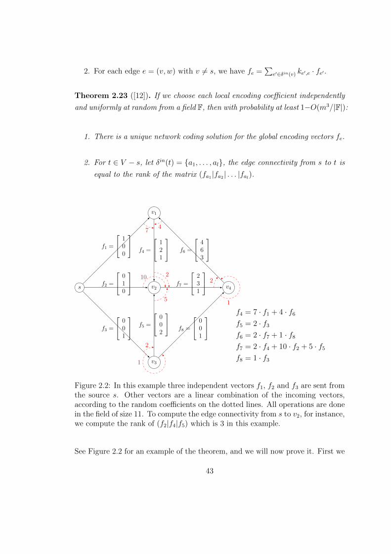
2. For each edge e = (v, w) with v 6= s, we have fe =∑

e′∈δin(v) ke′,e · fe′ .

Theorem 2.23 ([12]). If we choose each local encoding coefficient independently

and uniformly at random from a field F, then with probability at least 1−O(m3/|F|):

1. There is a unique network coding solution for the global encoding vectors fe.

2. For t ∈ V − s, let δin(t) = a1, . . . , al, the edge connectivity from s to t is

equal to the rank of the matrix (fa1|fa2| . . . |fal).

s

v1

v3

v2 v4

f1 =

100

f2 =

010

f3 =

001

f4 =

121

f5 =

002

f6 =

463

f7 =

231

f8 =

001

74

10

5

2

1

2

1

2

f4 = 7 · f1 + 4 · f6f5 = 2 · f3f6 = 2 · f7 + 1 · f8f7 = 2 · f4 + 10 · f2 + 5 · f5f8 = 1 · f3

Figure 2.2: In this example three independent vectors f1, f2 and f3 are sent fromthe source s. Other vectors are a linear combination of the incoming vectors,according to the random coefficients on the dotted lines. All operations are donein the field of size 11. To compute the edge connectivity from s to v2, for instance,we compute the rank of (f2|f4|f5) which is 3 in this example.

See Figure 2.2 for an example of the theorem, and we will now prove it. First we

43

rewrite the requirements of a network coding solution in a matrix form.

|

· · · fej · · ·|

=

|

· · · fej · · ·|

ke1,ej...

· · · kei,ej · · ·...

kem,ej

+

| | | |~e1 · · · ~ed ~0 · · · ~0

| | | |

Let F be the d × m matrix (fe1 | . . . |fem). Let K be the m × m matrix where

Ki,j = kei,ej when ei and ej are adjacent edges, and 0 otherwise. Let Hs be the

d×m matrix (~e1| . . . |~ed|~0|~0| . . . |~0) where ~0 denotes the all zero vector of dimension

d. Then the network coding equations are equal to the following matrix equation:

F = FK +Hs. (2.5.5)

To prove the first part of Theorem 2.23, we will prove in the following lemma

that (I −K) is non-singular with high probability. Then the above equation can

be rewritten as F = Hs(I−K)−1, which implies that the global encoding vectors

are uniquely determined.

Lemma 2.24 ([12]). Given the conditions in Theorem 2.23, the matrix (I −K)

is non-singular with probability at least 1−O(m/|F|).

Proof. Since the diagonal entries of K are zero, the diagonal entries of I − K

are all one. By treating each entry of K as an indeterminate Ki,j, it follows that

det(I − K) = 1 + p(· · · , Ki,j, · · · ) where p(· · · , Ki,j, · · · ) is a polynomial of the

indeterminates with total degree at most m. Note that det(I −K) is not a zero

polynomial since there is a constant term. Hence, by the Schwartz-Zippel Lemma,

if each Ki,j is a random element in F, then det(I −K) = 0 with probability at

most O(m/|F|), proving the lemma.

After we obtained the global encoding vectors, we would like to show that the

edge connectivities can be determined from the ranks of these vectors. Consider

a vertex t ∈ V − s. Let δin(t) = a1, . . . , al and let Mt be the d × l matrix

44

(fa1|fa2| . . . |fal). Let the edge connectivity from s to t be λs,t. We prove in the

following lemma that rank(Mt) = λs,t with high probability.

Lemma 2.25 ([12]). Given the conditions of Theorem 2.23, we have rank(Mt) =

λs,t with probability at least 1−O(m2/|F|).

Proof. First we prove that rank(Mt) ≤ λs,t with high probability. The plan is

to show that the global encoding vector on each incoming edge of t is a linear

combination of the global encoding vectors in a minimum s-t cut with high prob-

ability. Consider a minimum s-t cut δin(T ) where T ⊂ V with s /∈ T and t ∈ Tand din(T ) = λs,t. Let E ′ = e′1, . . . , e′m′ be the set of edges in E with their

heads in T . Let λ = λs,t and assume δin(T ) = e′1, . . . , e′λ. See Figure 2.3a for

an illustration. Let F ′ be the d×m′ matrix (fe′1| . . . |fe′m′ ). Let K ′ be the m′×m′

submatrix of K restricted to the edges in E ′. Let H ′ be the d × m′ matrix

(fe′1| . . . |fe′λ|~0| . . . |~0). Then, by the network coding requirements, the matrices

satisfy the equation

F ′ = F ′K ′ +H ′.

By the same argument as in Lemma 2.24, the matrix (I−K ′) is nonsingular with

probability at least 1−O(m/|F|). So the above matrix equation can be rewritten

as F ′ = H ′(I − K ′)−1. This implies that every global encoding vector in F ′ is

a linear combination of the global encoding vectors in H ′, which are the global

encoding vectors in the cut δin(T ). Therefore the rank(Mt) ≤ din(T ) = λs,t.

Now we prove that rank(Mt) ≥ λs,t with high probability. The plan is to show

that there is a λ × λ submatrix M ′t of Mt such that det(M ′

t) is a non-zero poly-

nomial of the local encoding coefficients with small total degree. First we use the

edge disjoint paths from s to t to define M ′t . Let λ = λs,t and P1, . . . , Pλ be a

set of λ edge disjoint paths from s to t. Set ke′,e = 1 for every pair of adjacent

edges e′, e ∈ Pi for every i, and set all other local encoding coefficients to be zero.

See Figure 2.3b for an illustration. Then each path sends a distinct unit vector

of the standard basis to t, and thus Mt contains a λ × λ identity matrix as a

submatrix. Call this λ × λ submatrix M ′t . Next we show that the det(M ′

t) is

a non-zero polynomial of the local encoding coefficients with small total degree.

Recall that F = H(I −K)−1. By considering the adjoint matrix of I −K, each

45

s

t T

fe′1

fe′2 · · ·fe′λ

fe′i

(a) Upper bound by min-cut.

s

t

10

0

1

0

1 1

0

(b) Lower bound by paths.

Figure 2.3: Rank of vectors received related to connectivity.

entry of (I − K)−1 is a polynomial of the local encoding coefficients with total

degree m divided by det(I −K), and thus the same is true for each entry of F .

Hence det(M ′t) is a degree λm polynomial of the local encoding coefficients divided

by (det(I − K))λ. By using the edge disjoint paths P1, . . . , Pλ, we have shown

that there is a choice of the local encoding coefficients so that rank(M ′t) = λ.

Thus det(M ′t) is a non-zero polynomial of the local encoding coefficients. Con-

ditioned on the event that det(I − K) is nonzero, the probability that det(M ′t)

is nonzero is at most O(λm/|F|) ≤ O(m2/|F|) by the Schwartz-Zippel lemma.

This implies that M ′t is a full rank submatrix with high probability, and thus

rank(Mt) ≥ rank(M ′t) = λ. We conclude that rank(Mt) = λs,t with probability

at least 1−O(m2/|F|).

Thus the probability that rank(Mt) 6= λs,t for some t ∈ V − s is at most n ·O(m2/|F|) ≤ O(m3/|F|) by union bound on t, and this proves the second part

of Theorem 2.23. Therefore, we only need to pick a large enough field F so that

|F| = Ω(m4) to guarantee a high probability result.

Now we show that the matrix (I − K)−1 actually contains the information of

connectivities between all vertices.

Theorem 2.26 ([12]). The rank of the submatrix (I −K)−1δout(s),δin(t) gives the

s-t edge connectivity.

46

Proof. To solve F = FK + Hs, we compute (I − K)−1 and get F = Hs(I −K)−1. In our setup, Hs is a dout(s) ×m matrix with a dout(s) × dout(s) identity

matrix in the columns corresponding to δout(s). So F is just equal to ((I −K)−1)δout(s),∗ up to permuting rows. To compute the edge connectivity from s to

t, by Theorem 2.23 we compute the rank of F∗,δin(t) and this is just equal to the

rank of ((I −K)−1)δout(s),δin(t).

Since I − K is an m × m matrices, its inverse can be computed in O(mω)

time. Given vertices s and t, computing the rank of ((I −K)−1)δout(s),δin(t) takes

O(dout(t)(dout(s))ω−1) time. So the total time to compute the ranks of the required

submatrices for all s and t is∑s∈V

∑t∈V

O(dout(t)(dout(s))ω−1) =∑s∈V

O(m · (dout(s))ω−1) = O(mω).

Thus the total time to compute edge connectivities between all s and t is O(mω)

time. In Chapter 4 we will show that (I−K)−1 can be computed more efficiently

in graphs with good separators.

47

48

Chapter 3

Linear Matroid Parity

The results presented in this chapter are based on joint work with Lap Chi Lau

and Kai Man Leung [11].

3.1 Introduction

The graph matching problem and the matroid intersection problem are two

fundamental polynomial-time solvable problems in combinatorial optimization.

Several efforts have been made to obtain an elegant common generalization of

these two problems, e.g. the matroid parity problem by Lawler [39] (equivalent

to the matchoid problem by Edmonds [34] and the matroid matching problem

by Lovasz [42]), the optimal path-matching problem by Cunningham and Gee-

len [16], and the membership problem for jump system by Bouchet and Cunning-

ham [5, 43].

So far the matroid parity problem is the most-studied and the most fruitful prob-

lem among these generalizations. Although it is shown to be intractable in the

oracle model [35] and is NP-hard for matroids with compact representations [42],

Lovasz [42] proved an exact min-max formula and obtained a polynomial time

algorithm for the linear matroid parity problem.

This provides a polynomial-time solvable common generalization of the graph

49

matching problem and the linear matroid intersection problem. Moreover, the

linear matroid parity problem has many applications of its own in various ar-

eas, including the path packing problem [46, 63] in combinatorial optimization,

the minimum pinning set problem [42, 36] in combinatorial rigidity, the maxi-

mum genus imbedding problem [20] in topological graph theory, the graphic ma-

troid parity problem [42, 22] used in approximating minimum Steiner tree [59, 3]

and approximating maximum planar subgraph [8], and the unique solution prob-

lem [44] in electric circuit.

Given its generality and applicability, it is thus of interest to obtain fast algo-

rithms for the linear matroid parity problem. In this paper we will present faster

and simpler algorithms for the linear matroid parity problem, and also improved

algorithms for specific graph problems of interest. The algorithms are based on

the algebraic algorithmic framework developed by Mucha and Sankowski [48],

Harvey [30, 28], and Sankowski [61].

3.1.1 Problem Formulation and Previous Work

The linear matroid parity problem can be formulated as follows without using

terminology from matroid theory: given an r × 2m matrix whose columns are

partitioned into m pairs, find a maximum cardinality collection of pairs so that

the union of the columns of these pairs are linearly independent. For instance,

to formulate the graph matching problem as a linear matroid parity problem, we

construct an n× 2m matrix where the rows are indexed by the vertices and the

pairs are indexed by the edges, where an edge ij is represented by two columns

where one column has an 1 in the i-th entry and 0 otherwise and the other column

has an 1 in the j-th entry and 0 otherwise.

There are several deterministic combinatorial algorithms for the linear matroid

parity problem. The first polynomial time algorithm is obtained by Lovasz with

a running time of O(m17) which can be implemented to run in O(m10) time [42,

44]. The fastest known algorithm is an augmenting path algorithm obtained by

Gabow and Stallmann [23] with running time O(mrω) [63], where ω ≈ 2.376

is the exponent on the running time of the fastest known matrix multiplication

50

algorithm [14]. Orlin and Vande Vate [55] presented an algorithm with running

time O(mrω+1) [63] by reducing it to a sequence of matroid intersection problems.

Recently Orlin [54] presented a simpler algorithm with running time O(mr3).

While these algorithms are all deterministic and reveal substantial structural

insights into the problem, even the simplest algorithm by Orlin is quite complex

and probably too difficult to implement in practice.

On the other hand, Lovasz [41] proposed an algebraic approach to the linear

matroid parity problem. First, he constructed an appropriate matrix with inde-

terminates (variables) where the matrix is of full rank if and only if there are r/2

linearly independent pairs (see Section 2.9). Then he showed that determining

whether the matrix is of full rank can be done efficiently with high probabil-

ity, by substituting the variables with independent random values from a large

enough field, and then computing the determinant of the resulting matrix [41].

This approach can be easily modified to determine the optimal value of the linear

matroid parity problem in one matrix multiplication time, and one can also con-

struct a solution in m matrix multiplications time. Note that this already gives

a randomized O(mrω)-time algorithm for the linear matroid parity problem, and

this algebraic approach also leads to an efficient parallel algorithm for the linear

matroid parity problem [52].

In a recent line of research an elegant algorithmic framework has been developed

for this algebraic approach. Mucha and Sankowski [48] showed how to use Gaus-

sian eliminations to construct a maximum matching in one matrix multiplication

time, leading to an O(nω) time algorithm for the graph matching problem where

n is the number of vertices. Harvey [30] used a divide-and-conquer method to

obtain an algebraic algorithm for the linear matroid intersection problem with

running time O(mrω−1) where m is the number of columns, and a simple O(nω)

time algorithm for the graph matching problem. Furthermore, Sankowski [61] and

Harvey [28] extended the algebraic approach to obtain faster pseudo-polynomial

algorithms for the weighted bipartite matching problem and the weighted linear

matroid intersection problem.

Besides matching and linear matroid intersection, other special cases of the lin-

ear matroid parity problem have also been studied. One special case of interest

51

is the graphic matroid parity problem [22, 24, 66, 67], which has applications

in designing approximation algorithms [8, 59, 3]. For this problem the fastest

known algorithm is by Gabow and Stallmann [22] which runs in O(mn lg6 n)

time. Another special problem of considerable interest is Mader’s S-path packing

problem [46, 42, 64, 13, 56, 57, 58, 2] which is a generalization of the graph match-

ing problem and the s-t vertex disjoint path problem. Lovasz [42] showed that

this problem can be reduced to the linear matroid parity problem. Chudnovsky,

Cunningham and Geelen [13] obtained an O(n6) time direct combinatorial algo-

rithm for the problem, and Pap [58, 57] obtained a simpler direct combinatorial

algorithm for the problem and also for the more general capacitated setting.

3.1.2 Our Results

We obtain fast and simple algebraic algorithms for the linear matroid parity

problem and also for some specific graph problems of interest. All algorithms are

best possible in the sense that either they match the running time in well-known

special cases or they are optimal in terms of some parameters.

Linear Matroid Parity

There are two algebraic formulations for the linear matroid parity problem, one

is a “compact” formulation by Lovasz in Theorem 2.9 and another is a “sparse”

formulation by Geelen and Iwata in Theorem 2.10. Using the compact formu-

lation and the Sherman-Morrison-Woodbury formula, we present a very simple

algorithm for the linear matroid parity problem.

Theorem 3.1. There is an O(mr2)-time randomized algorithm for the linear

matroid parity problem.

One feature of this algorithm is that it does not use fast matrix multiplication

and is very easy to be implemented in practice. Note that it is already faster than

the Gabow-Stallmann O(mrω) time algorithm, and actually if fast matrix multi-

plication is not used then the best known algorithms run in O(mr3) time [23, 54].

Using the divide-and-conquer method of Harvey [30] on the sparse formulation

52

and fast matrix multiplications, we can improve the running time further to match

the running time of the linear matroid intersection problem, answering a question

of Harvey [30].

Theorem 3.2. There is an O(mrω−1)-time randomized algorithm for the linear

matroid parity problem.

It is still open whether there is a polynomial time algorithm for the weighted linear

matroid parity problem, and even a deterministic PTAS is not known yet [40].

We present a faster pseudo-polynomial randomized algorithm for the weighted

matroid parity problem, which also implies a faster randomized FPTAS for the

weighted linear matroid parity problem using standard scaling technique [59].

Graph Algorithms

For graph problems that can be reduced to the linear matroid parity problem, we

show that the additional structure can be exploited in the compact formulation

to obtain faster algorithms than that follow from Theorem 3.2. We illustrate this

with some well-known problems.

Mader’s Disjoint S-Path In this problem we are given an undirected graph

G = (V,E) and S is a collection of disjoint subsets of V . The goal is to find

a maximum collection of vertex disjoint S-paths, where an S-path is a path

that connects two different sets in S and has no internal vertex in S. This

problem generalizes the graph matching problem and the vertex disjoint s-t path

problem, and is of considerable interest [46, 42, 64, 13, 56, 57, 58, 2]. Obtaining

a direct combinatorial algorithm is quite nontrivial [13, 58]. The best known

running time is still the O(mnω)-time bound implied by the Gabow-Stallmann

algorithm, where m is the number of edges and n is the number of vertices.

The algorithm in Theorem 3.2 implies an O(mnω−1)-time algorithm. By using

the compact formulation, we further improve the running time to match the

algebraic algorithms for the graph matching problem. The algorithm would be

quite simple if fast matrix multiplication is not used, and its running time would

be O(n3) which is still faster than the existing algorithms.

53

Theorem 3.3. There is an O(nω)-time randomized algorithm for Mader’s S-path

problem.

Graphic Matroid Parity In this problem we are given an undirected graph

and some edge pairs, and the problem is to find a maximum collection of edge

pairs such that the union of these edges forms a forest. One special case of

interest [44, 66] is when each pair has a common vertex (i.e. ij, ik for some

vertex i). This has applications in approximating minimum Steiner tree [59, 3]

and approximating maximum planar subgraph [8]. In the general problem the

input could have up to Ω(n4) edge pairs where n is the number of vertices, and

in the special problem the number of edge pairs could be Ω(n3). The following

algorithms achieve optimal running time in terms of n for both problems.

Theorem 3.4. There is an O(n4)-time randomized algorithm for the graphic

matroid parity problem, and an O(n3)-time randomized algorithm when each edge

pair has a common vertex.

The fastest algorithm on graphic matroid parity is obtained by Gabow and Stall-

mann [22] with running time O(mn lg6 n) where m is the number of edge pairs,

and so our algorithm is faster if there are Ω(n3) edge pairs in the general problem

and if there are Ω(n2) edge pairs in the special problem. We remark that the

same statement holds even if we use a cubic algorithm for matrix multiplication,

and the resulting algorithm is much simpler than that of Gabow and Stallmann.

Colorful Spanning Tree In this problem we are given an undirected multi-

graph G = (V,E) where each edge has one color, and the objective is to determine

whether there is a spanning tree in which every edge has a distinct color. This

is a generalization of the arborescence problem and the connected detachment

problem [53, 63], and is a special case of the linear matroid intersection prob-

lem. Note that the input graph could have Ω(n3) edges where n is the number

of vertices, since each pair of vertices could have Ω(n) edges in between, each of

which has a distinct colors. So the following algorithm has optimal running time

in terms of n.

54

Theorem 3.5. There is an O(n3)-time randomized algorithm for the colorful

spanning tree problem.

3.1.3 Techniques

Our results show that both the algebraic algorithms for graph matching and linear

matroid intersection can be generalized to linear matroid parity. The O(mrω−1)-

time algorithm for linear matroid parity is a straightforward generalization of

Harvey’s linear matroid intersection algorithm, and the algorithm for weighted

linear matroid parity follows from the techniques used by Sankowski [61]. The

main new technical contribution is the use of the compact formulation to design

new algebraic algorithms. For graph problems, the basic observation is that the

column vectors have at most a constant number of nonzeros, and this allows

us to extend Harvey’s matching algorithm to obtain faster algorithms using the

compact formulation. The O(nω) algorithm for the S-path problem is based on a

good matrix formulation of the problem, while the O(n3) algorithms for graphic

matroid parity and colorful spanning tree are based on different recursions used in

the divide-and-conquer method. We remark that this approach on the compact

formulation implies some new results for linear matroid intersection problems

as well, e.g. colorful spanning tree, graphic matroid intersection, simple O(mr2)

algorithm.

While linear matroid parity and Mader’s disjoint S-path are challenging gener-

alizations for the design of combinatorial algorithms, our results show that the

algebraic algorithmic framework can be adapted nicely to give faster and sim-

pler algorithms in more general settings. Our algorithms are still faster than the

existing algorithms even if fast matrix multiplications are not used, and these

simpler algorithms could be implemented easily in practice using MATLAB (see

e.g. [29]).

Organization In Section 3.3, we will give the proof of Theorem 3.1. Then we

will present graph algorithms for Mader’s Disjoint S-path problem, the graphic

matroid parity problem and the colorful spanning tree problem in Section 3.4.

55

The results on weighted linear matroid parity will be presented in Section 3.5,

and the proof of Theorem 3.2 will be presented in Section 3.6.

3.2 Preliminaries

When a set of integers S are partitioned into k subsets, the set S is partitioned

into k equal size subsets S1, S2, · · ·Sk. In addition, S1 contains the smallest |S|/kelements of S, S2 contains the next |S|/k smallest elements of S, and Sk contains

the largest |S|/k elements of S.

We assume the number of pairs m and the number of rows r in the linear matroid

parity problem will be powers of two. This assumption can be easily satisfied by

adding redundant pairs and rows.

3.3 A Simple Algebraic Algorithm for Linear

Matroid Parity

In this section we will present a matrix formulation and a simple O(mr2) time

algorithm for the linear matroid parity problem.

Given an r × 2m matrix M where the columns are partitioned into m pairs

b1, c1, . . . , bm, cm, the linear matroid parity problem is to find a maximum

collection of pairs J ⊆ [m] so that the vectors in⋃i∈Jbi, ci are linearly inde-

pendent. We use νM to denote the optimal value, and call an optimal solution

a parity basis if νM = r/2. We also call a set parity set if every column pair is

either contained in it or disjoint from it.

3.3.1 An O(mr2) Algorithm

In this subsection we present a very simple O(mr2)-time algorithm for the linear

matroid parity problem. Here we consider the case where we find a parity basis

56

if one exists or report that no parity basis exists. We will show how to reduce

the general problem to this case in Section 3.7.

A pseudocode of the algorithm is presented in Algorithm 3.1. First we construct

the matrix Y with indeterminates using the compact formulation in Theorem 2.9.

Theorem 2.9. Given m column pairs (bi, ci) for 1 ≤ i ≤ m and bi, ci ∈ Rr.

Let

Y =m∑i=1

xi(bi ∧ ci),

where xi are indeterminates. Then 2νM = rank(Y ).

By Theorem 2.9 we have νM = r/2 if and only if Y is of full rank. As stated

in Section 3.2, we can test whether Y is of full rank in O(r3) time with high

probability, by substituting the indeterminates with random values and then

checking whether the resulting matrix has nonzero determinant. If Y is not of

full rank, then we report that no parity basis exists, otherwise we construct the

matrix Y −1 in O(r3) time.

Then, for each column pair (bi, ci), the algorithm checks whether this pair can be

removed while keeping the resulting matrix full rank. If so this pair is removed

from the problem since there is still an optimal solution surviving, otherwise this

pair is kept since it is in every parity basis with high probability. In the end the

algorithm returns the pairs that were not removed.

Next we show how to check whether a pair can be removed efficiently. First we

recall Theorem 2.15.

Theorem 2.15 (Sherman-Morrison-Woodbury). Let M be an n × n matrix, U

be an n× k matrix, and V be an n× k matrix. Suppose that M is non-singular.

Then

1. M + UV T is non-singular if and only if I + V TM−1U is non-singular.

2. If M + UV T is non-singular, then (M + UV T )−1 = M−1 − M−1U(I +

V TM−1U)−1V TM−1.

57

Removing the i-th column pair from M is equivalent to assign xi to zero. Let Y ′

be the new matrix with xi = 0, then

Y ′ = Y − xi(bicTi − cibTi ) = Y − xi(bi ci

)(ci -bi

)TObserve that this is just a rank-2 update. By setting U = xi

(bi ci

)and V =(

-ci bi

)and using Theorem 2.15(1), Y ′ is of full rank if and only if I+V TY −1U

is of full rank. Since both U and V are of size r × 2, we can check whether a

pair can be removed in O(r2) time. If so, we apply Theorem 2.15(2) to compute

the inverse of Y ′ by the formula Y −1 − Y −1U(I + V TY −1U)−1V TY −1, this can

be computed in O(r2) time since I + V TY −1U is of size 2 × 2. Applying this

procedure iteratively, the whole algorithm can be implemented in O(mr2) time.

Finally the algorithm fails only if a matrix is of full rank but the determinant is

zero after the random substitutions. As stated in Section 3.2, this happens with

probability at most r/q where q is the field size. Since we only check the rank at

most m times, the failure probability is at most mr/q by the union bound, and

so by choosing q = mr/ε this probability is at most ε.

Algorithm 3.1 A simple algebraic algorithm for linear matroid parity

SimpleParity(M)Construct Y using the compact formulation and assign random values toindeterminates xiif det(Y ) = 0 return “there is no parity basis”Compute Y −1

Set I = b1, c1, · · · bm, cmfor i = 1 to m do

Set Y ′ := Y − xi(bi ci

) (ci -bi

)Tif det(Y ′) 6= 0 thenY := Y ′

Update Y −1 by the Sherman-Morrison-Woodbury formulaI := I − bi, ci

return I

58

3.4 Graph Algorithms

In most applications of linear matroid parity, not only is the given matroid a linear

matroid, but also each column vector of the matroid has few nonzero entries. For

example, each column vector of a graphic matroid has only two nonzero entries.

In this section, we will show how we can exploit such special structure to obtain

faster algorithms for some graph problems of interest.

For Mader’s S-path problem in Section 3.4.1, we will translate the reduction into

a good matrix formulation, so that the recursive approach for graph matching

problem can be extended to solve this problem. Also, we will give different

recursive algorithms to solve the graphic matroid parity problem in Section 3.4.2

and the colorful spanning tree problem in Section 3.4.3.

Our algorithms below assume the matroid parity instance contains a parity basis.

If not we can use the approach to be described in Section 3.7 to reduce to this

case: Suppose the given linear matroid M has r rows. Consider the matrix

formulation Y in Theorem 2.9. The maximum rank submatrix YS,S can be found

in O(rω) time, and then we only need to focus on YS,S. At any time our algorithm

considers a submatrix YR,C , we shall consider YR∩S,C∩S instead.

3.4.1 Mader’s S-Path

Given an undirected graph G = (V,E) and let S1, · · · , Sk be disjoint subsets of V .

A path is called an S-path if it starts and ends with vertices in Si and Sj such that

Si 6= Sj, while all other internal vertices of the path are in V \(S1∪S2∪ · · · ∪Sk).The disjoint S-path problem is to find a maximum cardinality collection of vertex

disjoint S-Paths of the graph G. In the following we assume without loss of

generality that each Si is a stable set.

Lovasz [42] showed that the S-path problem can be reduced to the linear matroid

parity problem, but it is not immediately clear how his reduction can be translated

into a matrix formulation of the problem. Instead, we will follow the reduction by

Schrijver ([63] page 1284), and show that it can be translated into a good matrix

formulation.

59

Reduction to Linear Matroid Parity

Here we first recall the reduction from Section 2.1.4. The high level idea is to as-

sociate each edge to a 2-dimensional linear subspace, and show that the edges in

a solution of the S-path problem correspond to subspaces that are linearly inde-

pendent in an appropriately defined quotient space R2n/Q, where two subspaces

are linearly independent if their basis vectors are linearly independent.

Associate each edge e = (u,w) ∈ E to a 2-dimensional linear subspace Le of

(R2)V such that

Le =x ∈ (R2)V | x(v) = 0 for each v ∈ V \u,w and x(u) + x(w) = 0

where x : V → R2 is a function that maps each vertex to a 2-dimensional vector.

Let r1, · · · rk be k distinct 1-dimensional subspaces of R2. For each vertex v ∈ V ,

let Rv = rj if v ∈ Sj for some j, and Rv = 0 otherwise. Define a linear subspace

Q of (R2)V such that

Q = x ∈ (R2)V | x(v) ∈ Rv for all v ∈ V .

Let E be the collection of subspaces Le/Q for each e ∈ E of (R2)V /Q, where

Le/Q is the quotient space of Le by Q. Note that dim(Le/Q) = 2 for all edges

e, since it does not connect two vertices in the same Si as we assume each Si is

a stable set. In Theorem 2.2 we proved the following theorem which shows the

reduction to the linear matroid parity problem.

Theorem 2.2. If G is connected, then the maximum number of disjoint S-paths

is equal to ν(E)−|V |+ |T |, where T =⋃ki=1 Si and ν(E) is the size of a maximum

collection of linearly independent 2-dimensional subspaces in E.

Matrix Formulation

To translate the above reduction into a matrix formulation, we need to associate

each edge e to a column pair (b′e, c′e), such that for F ⊆ E the subspaces in

LF = Le/Q | e ∈ F are linearly independent if and only if the vectors in

60

⋃e∈Fb′e, c′e are linearly independent.

Let ~ek be the k-th unit vector. For each edge e = (u, v) ∈ E, construct an

orthogonal basis be and ce of Le such that

be = ~e2u−1 − ~e2v−1 and ce = ~e2u − ~e2v,

where we abuse notation to also use u and v as indices of the vertices u and v.

For v ∈ V we define:

qv =

~e2v−1 + i~e2v if v ∈ Si0 otherwise

Note that the collection of non-zero qv forms an orthogonal basis of Q. To obtain

the vectors for Le/Q, we just need to write be = b′e + bQ and ce = c′e + cQ

where b′e, c′e ∈ Q⊥ and bQ, cQ ∈ Q. Then, for any subset F ⊆ E, the vectors

in⋃e∈Fbe, ce are linearly independent in R2n/Q if and only if the vectors in⋃

e∈Fb′e, c′e are linearly independent in R2n.

We can use a procedure similar to the Gram-Schmidt process to compute (b′e, c′e)

from (be, ce). Recall that the collection of non-zero qv forms an orthogonal basis

of Q. Define

b′e = be −∑

v∈V :qv 6=0

bTe qvqTv qv

qv c′e = ce −∑

v∈V :qv 6=0

cTe qvqTv qv

qv.

By subtracting the projection of be onto qv for all v from be, the resulting vector

b′e is orthogonal to the subspace Q. Thus, by the above discussion, we have that

for each F ⊆ E, the subspaces in LF = Le/Q | e ∈ F are linearly independent

if and only if the vectors in⋃e∈Fb′e, c′e are linearly independent in R2n.

Therefore, by solving the linear matroid parity problem on the set of column pairs

(b′e, c′e) for all e ∈ E, we can find the maximum number of disjoint S-paths in G,

using Theorem 2.2. Also, from the solution of the linear matroid parity problem,

one can easily construct the solution for the S-path problem, (see Section 2.1.4).

Observe that for any e = (u, v), after the Gram-Schmidt process, b′e and c′e are of

61

the form:

b′e =i2

1 + i2~e2u−1 −

i

1 + i2~e2u −

j2

1 + j2~e2v−1 +

j

1 + j2~e2v

c′e = − i

1 + i2~e2u−1 +

1

1 + i2~e2u +

j

1 + j2~e2v−1 −

1

1 + j2~e2v

where u ∈ Si and v ∈ Sj for some i and j. If u or v are not in any Si, then the

corresponding entries in b′e and c′e remain the same as in be and ce. Therefore,

M contains at most four non-zero entries in each column. Now we can apply

Theorem 2.9 to construct the described matrix Y for the linear matroid parity

problem, which is given by Y =∑

e∈E xe(b′e ∧ c′e).

Let m = |E| and n = |V |. Then Y is a 2n× 2n matrix. For each wedge product,

there are at most four 2× 2 non-zero blocks, and so for each edge e there are at

most 16 entries of xe in Y . Further observe that for any 2× 2 non-zero block at

the two rows occupied by u and two columns occupied by v of Y , the same block

(but negated) appears at the two rows occupied by v and two columns occupied

by u of Y . Hence the appearance of 2 × 2 blocks (as well as the indeterminates

xi) are always symmetric.

Recursive Algorithm

Our algorithm is a direct generalization of Harvey’s graph matching algorithm

discussed in Section 2.4.3. Here is the high-level idea of the recursive algorithm

to construct a parity basis of M . Similar to the O(mr2)-time algorithm in Sec-

tion 3.3, the algorithm checks for each edge e whether some parity basis survives

after the column pair (b′e, c′e) is removed. Removing a column pair (b′e, c

′e) is equiv-

alent to setting the corresponding xe to zero. The observation is that each edge e

has at most 16 entries of xe in Y , and so the small area update formula of Harvey

can be applied. Recall Theorem 2.16:

Theorem 2.16 (Harvey). Let M be a non-singular matrix and let N = M−1. Let

M be a matrix which is identical to M except MS,S 6= MS,S and let ∆ = M −M .

1. M is non-singular if and only if det(I + ∆S,SNS,S) 6= 0.

62

2. If M is non-singular then M−1 = N −N∗,S(I + ∆S,SNS,S)−1∆S,SNS,∗.

3. Restricting M−1 to a subset T , we have

M−1T,T = NT,T −NT,S(I + ∆S,SNS,S)−1∆S,SNS,T ,

which can be computed in O(|T |ω) time for |T | ≥ |S|.

Suppose we already have Y and Y −1, this implies that checking whether e can

be removed can be done in constant time by Theorem 2.16(1). Note that we also

need to update Y −1 for future queries, and therefore we use a recursive procedure

so that edges within a subset are removed consecutively, so that the relevant

entries in the inverse can be computed more efficiently using Theorem 2.16(3).

The algorithm is shown in Algorithm 3.2. Let R and C be the indices of a subset

of rows and a subset of columns of Y , and S = R ∪ C. For each edge e = uv,

the corresponding xe appears only in YTe,Te where Te = 2u − 1, 2u, 2v − 1, 2v.Procedure Remove(R,C) will try to remove all edges e = uv with Te ⊆ S. In the

base case when |R| = |C| = 2, we can determine whether xe can be eliminated

or not by Theorem 2.16(1) in constant time. Otherwise, when |R| = |C| > 2, we

partition R and C into R1, R2 and C1, C2, such that first(second) half of R goes

to R1(R2), and C is also partitioned in the same way. And then we recursively

call Remove(Ri, Cj) for i, j ∈ 1, 2. Note that before entering into any smaller

area during the recursion, we need to update Y −1, but only updating Y −1S,S is

enough for the checkings in Remove(Ri, Cj) by Theorem 2.16(1), and this can

be done in O(|S|ω) time using Theorem 2.16(3).

Correctness: The algorithm is correct because every pair is checked, and when

a pair is checked the relevant entries in the inverse are always updated. Consider

an instance of Remove on rows R and columns C and let S = R ∪ C. We

keep the invariant NS,S = Y −1S,S. After each recursive call Remove(Ri, Cj) for

i, j ∈ 1, 2, only the entries in YS,S have been changed, denoted by ∆S,S. By The-

orem 2.16(3), NS,S can be updated by NS,S−NS,S(I+∆S,SNS,S)−1∆S,SNS,S, which

can be done in O(|S|ω) time. When a base case is reached, by Theorem 2.16(1),

an indeterminate x can be removed if and only if det(I+∆S,SNS,S) 6= 0, which can

63

be checked in constant time since |S| = 4. The analysis of the failure probability

is the same as in Section 3.3.1 and we omit it here.

Time Complexity: Let f(n) be the time required by Remove, where n =

|R| = |C|. From Algorithm 3.2 we have f(n) = 4f(n/2)

+ O(nω). Hence we

have f(n) = O(nω) by the master theorem [15]. The initialization also takes time

O(nω), and so the overall time complexity is O(nω).

Algorithm 3.2 An algebraic algorithm for disjoint S-paths

Spath(M)Construct Y and assign random values to each indeterminate xe for e ∈ ECompute N := Y −1 by a fast inverse algorithmRemove(1..2n, 1..2n)return all remaining pairs

Remove(R,C)Let S = R ∪ CInvariant: NS,S = Y −1S,Sif |R| = |C| = 2 then

Let e = uv be the edge (if exists) with S = 2u− 1, 2u, 2v − 1, 2vLet xe and b′e, c

′e be the indeterminate and the vectors associated with e

Set Y ′ = Y − xe(b′e ∧ c′e)Check if Y ′ is non-singular by the small area update formula (Theo-rem 2.16(1))if Y ′ is non-singular then

Remove e and set Y = Y ′

elsePartition R and C into two equal-size subsetsfor all pairs i, j ∈ 1, 2 doRemove(Ri, Cj)Compute NS,S = Y −1S,S by the small area update formula (Theo-rem 2.16(3))

3.4.2 Graphic Matroid Parity

In this problem we are given an undirected graph and some edge pairs, and the

problem is to find a maximum collection of edge pairs such that the union of these

edges forms a forest. In some applications for graphic matroid parity, each of the

64

given edge pair has a common vertex. We will first show an O(n3) time algorithm

for this special case, followed by an O(n4) time algorithm for the general case.

Construct the matrix Y using the compact formulation in Theorem 2.9. Since

the matroid is graphic, there are only two nonzero entries in each bi and ci. Let

each bi and ci be written in the form ~ej − ~ek and ~eu − ~ev where jk is one edge

and uv is another edge. It is easy to see that each pair of elements affects at

most 8 entries in Y , and thus the small area update formula can be used. Similar

to previous sections, we use a recursive approach to enumerate each edge pair.

For each pair our algorithm checks if some parity basis survives after removal of

such pair. Recall that a parity basis exists if and only if its corresponding matrix

formulation Y is of full rank. Removing a pair is done by assigning corresponding

xi to zero. Since xi affects at most 8 entries, this can be checked in constant time

by Theorem 2.16(1) using Y −1. If Y remains full rank after setting xi to zero, we

remove such pair. When the algorithm terminates, the remaining pairs forms a

parity basis.

We first consider the special case where each edge pair has a common vertex,

where we can obtain a speedup over the general graphic matroid parity problem.

The algorithm is shown in Algorithm 3.3. Define procedure Remove(P,R,C)

to check all edge pairs (i, j), (i, k) that have i ∈ P , j ∈ R and k ∈ C. Consider

the base case where |P | = |R| = |C| = 1. We need to determine whether pair

(i, j),(i, k) (i ∈ P , j ∈ R, k ∈ C) can be removed. Since removal of such pair

will only affect entries in YS,S where S = P ∪R ∪C, decision can be made using

Theorem 2.16(1) in constant time using Y −1S,S.

The algorithm start with Remove(V, V, V ), V = 1..n, which will check all

edge pairs. The procedure simply calls recursions when it does not reach its

base cases yet. For any set T , define its first (second) half by T1 (T2). Then

the procedure can be implemented by recursive call to Remove(Px, Ry, Cz) for

all x, y, z ∈ 1, 2. Since inverse of Y is required to decide if a pair can be

removed, Y −1S,S (S = P ∪R ∪C) is recomputed before each recursive call using

Theorem 2.16(3), as in the algorithm for the S-path problem.

Now we analyze the time complexity of this algorithm. Any changes done by

Remove(P,R,C) is made to YS,S where S = P ∪ R ∪ C. So, similar to that

65

in the S-path problem, updating Y −1S,S using Theorem 2.16(3) takes O(|S|ω)

time. Let f(n) be time required by Remove where n = |P | = |R| = |C|.We have f(n) = 8f(n/2) + O(nω). By the master theorem [15], if fast matrix

multiplication is used, this algorithm has overall time complexityO(n3), otherwise

its time complexity is O(n3 log n) time. The analysis of the failure probability is

the same as in Section 3.3.1 and we omit it here.

For the general case where edge pairs are in the form (i, k) and (j, l). Our algo-

rithm is very similar but the procedure is now defined as Remove(P,Q,R,C)

which checks all pairs in the form i ∈ P , j ∈ Q, k ∈ R and l ∈ C. Hence we now

require 16 recursion calls of Remove(Pw, Qx, Ry, Cz) where w, x, y, z ∈ 1, 2.This gives an O(n4) time algorithm by the master theorem.

3.4.3 Colorful Spanning Tree

Given an connected undirected multigraph G = (V,E) where each edge is colored

by one of the k ≤ n colors. The colorful spanning tree problem [63] is to determine

if there is a spanning tree T in G such that each edge in T has a distinct color.

Let n = |V | and m = |E|.

The tree constraint can be captured by a graphic matroid M1, where an edge

(u, v) is represented by a column vector ~eu − ~ev. So a set of edges are acyclic if

and only if their vectors for M1 are independent. The distinct color constraint can

be modeled by a partition matroid M2, where an edge with color d is represented

by a column vector ~ed. So a set of edges have distinct colors if and only if their

vectors for M2 are independent.

Thus a maximum cardinality common independent set of M1 and M2 gives a

maximum size acyclic colorful subgraph of G. In particular when k = n− 1 and

G is connected, a common basis of the two matroids is a colorful spanning tree

of G. We show how to reduce the problem to the linear matroid parity problem.

For each edge e = (u, v) with color d, construct a column pair as follows. Let be

and ce have size 2n× 1. Set the first half of be to be ~eu−~ev, the second half of ce

to be ~ed, and ~0 for remaining half of be and ce. Now each bi is independent with

any cj. Hence a parity set is independent if and only if the corresponding edges

66

Algorithm 3.3 An algebraic algorithm for graphic matroid parity, when eachedge pair has a common vertex.

GraphicParity(M)Construct Y and assign random values to indeterminates xiN := Y −1

Remove(1..n, 1..n, 1..n)return all remaining pairs

Remove(P,R,C)Let S = P ∪R ∪ CInvariant: NS,S = Y −1S,Sif |P | = |R| = |C| = 1 then

Let i ∈ P , j ∈ R, k ∈ CLet x, b, c be the indeterminate and the vectors associated with edge pair(i, j) and (i, k) (if exists)Y ′ = Y − x(b ∧ c)Check if Y ′ is non-singular by the small area update formula (Theo-rem 2.16(1))if Y ′ is non-singular then

Remove this edge pair and set Y = Y ′

elsePartition P , R and C into two equal-size subsetsfor all tuples i, j, k ∈ 1, 2 doRemove(Pi, Rj, Ck)Compute NS,S = Y −1S,S using the small area update formula (Theo-rem 2.16(3))

67

form a colorful subgraph.

The idea of the algorithm is to examine each edge e one by one, and see if any

parity basis (that is a colorful spanning tree) remains after removal of this edge.

We construct Y as described in Theorem 2.9. Then each xi will only appear

in four entries because bicTi has only two non-zero entries. Let Y ′ be the new

matrix with xi assigned to zero, which is equivalent to remove edge ei. Let

S = u, v, d + n, Y ′ is identical to Y except Y ′S,S. Recall that we can remove

edge ei if the rank of Y ′ remains the same. If so we simply remove that edge and

update Y −1. After checking all edges a parity basis remains. If the size of the

parity basis is n− 1, then it is a colorful spanning tree.

One technical point is that we require Y to have full rank before the checking

starts. In our problem the originally constructed matrix Y is never of full rank.

So we need another matrix that gives the same result as Y while having full

rank. We will describe in Section 3.7 how to find such a matrix in Section 3.7.

Henceforth we assume that Y is of full rank.

The algorithm is shown in Algorithm 3.4, which is similar to that for the graphic

matroid parity problem. Let R be subset of rows of Y , C and C ′ be subset

of columns of Y . Define procedure Remove(R,C,C ′), which tries to remove

edges connecting u and v having color d that have (d + n) ∈ R, u ∈ C, v ∈ C ′.Remove(R,C,C ′) has |R| = |C| = |C ′| = 1 as base case, where we have to

determine whether a particular edge (u, v) having color d can be removed ((d +

n) ∈ R, u ∈ C, v ∈ C ′). This can be done in constant time using Theorem 2.16(1)

because removing such edge only affect four entries in Y . In other cases, R, C

and C ′ are partitioned into R1, R2, C1, C2 and C ′1, C′2. All eight smaller cases

Remove(Ri, Cj, C′k) will be called, where i, j, k ∈ 1, 2. After any recursive

call Y −1 is updated using Theorem 2.16(3). Let S = R ∪ C ∪ C ′, any instance

of Remove(R,C,C ′) triggers updates to YS,S. The updating process takes only

O(|S|ω) time.

Time Complexity: Let f(n) be the time required by Remove, where n =

|R| = |C| = |C ′|. We have f(n) = 8f(n/2) + O(nω). Hence f(n) = O(n3) by

the master theorem. As a result, the algorithm has time complexity O(n3). If

fast matrix multiplication is not used, then the algorithm has time complexity

68

O(n3 log n) again by the master theorem.

Algorithm 3.4 An algorithm to compute colorful spanning tree

ColorfulSpanningTree(G)Construct Y and assign random values to indeterminates xiCompute N := Y −1 by fast inverseRemove(1..2n, 1..2n, 1..2n)return all remaining edges

Remove(R,C,C ′)Let S = R ∪ C ∪ C ′Invariant: NS,S = Y −1S,Sif |R| = |C| = |C ′| = 1 then

Let (d+ n) ∈ R, u ∈ C, v ∈ C ′Let x, b, c be the indeterminate and the vectors associated with edge (u, v)with color d (if exists)Y ′ = Y − x(b ∧ c)Check if Y ′ is non-singular by the small area update formula (Theo-rem 2.16(1))if Y ′ is non-singular then

Remove this edge and set Y = Y ′

elsePartition R, C and C ′ into two equal-size subsetsfor all tuples i, j, k ∈ 1, 2 doRemove(Ri, Cj, C

′k)

Compute NS,S = Y −1S,S using the small area update formula (Theo-rem 2.16(3))

3.5 Weighted Linear Matroid Parity

In the weighted matroid parity problem, each pair i is assigned a non-negative

weight wi, and the objective is to find a parity basis with maximum weight. In

Theorem 2.11 we saw Camerini et al. gave a compact matrix formulation for this

problem. Consider the matrix Y ∗ =∑m

i=1 xi(bi ∧ ci)ywi . The theorem says each

term of pf Y ∗ corresponds to a parity basis, and the degree of y in that term

corresponds to the weight to the parity basis.

69

This gives an algorithm for the weighted problem similar to Algorithm 3.1, but we

need to make sure that some parity basis with maximum weight is preserved. If

the maximum weighted parity basis have weight p, we want to calculate pf Y ∗ to

see if a term containing yp still remains. It can be achieved by finding det(Y ∗) and

look for a term that contains y2p because det(Y ∗) = pf(Y ∗)2 However calculating

its determinant may not be easy. Define W = maxiwi. Camerini et al. [9]

proposed an O(m2r2 +Wmr4) algorithm to find the parity basis with maximum

weight.

Now we show we can apply Theorem 2.21 by Storjohann to give a faster algorithm.

The theorem says that given a n × n polynomial matrix of degree d then its

determinant can be computed in O(nωd) time. By choosing a large enough field

F, we can check if removing each pair i (by assigning xi = 0) would affect the

parity basis with maximum weight, with high probability. If the degree of det(Y ∗)

does not drop after removal of a pair, then it can be removed. And removal of a

pair can be simply done by an update to Y ∗ in O(r2) time. Each time the checking

can be done in O(Wrω) time by Theorem 2.21, which dominates the updating

time. Calculating Y ∗ at the beginning takes O(mr2) time. Hence we can find a

parity basis with the maximum weight in O(Wmrω) time. The pseudocode of

the algorithm can be found in Algorithm 3.5.

Algorithm 3.5 An algebraic algorithm for weighted linear matroid parity

MaxWeightParity(M)Construct Y ∗ and assign random values to indeterminates xiJ := b1, c1, · · · bm, cmfor i = 1 to m doY := Y ∗ − xi(bi ∧ ci)ywiif degree of det(Y ) equals that of det(Y ∗) thenY ∗ := YJ := J − bi, ci

return J

Finally we describe how to obtain a randomized fully polynomial-time approxi-

mation scheme using the pseudo-polynomial algorithm by standard scaling tech-

nique [59]. Here we assume every column pair is contained in some parity basis.

This assumption can be satisfied by checking the rank of corresponding Z(J) as

70

in Theorem 3.7. If Z(J) is not full rank we discard the corresponding column

pair.

The idea is to scale the weight of each pair down and solve the new instance

using Algorithm 3.5. Given ε > 0, let K = εW/r. For each pair i scale its

weight to w∗i = bwi/Kc. Solve the new instance using Algorithm 3.5. This takes

O(bW/Kcmrω) = O(mrω+1/ε) time.

We will show the result of the scaled instance is an (1− ε)-approximation of the

original instance. Let J and O be pairs return by the above algorithm and the

optimal pairs respectively. Also denote original (scaled) weight of a set S by

w(S) (w∗(S)). We have w(O) − Kw∗(O) ≤ rK because for each pair in O at

most weight with value K is lost, and there are at most r/2 pairs chosen. Then

w(J) ≥ K · w∗(J) ≥ K · w∗(O) ≥ w(O)− rK = w(O)− εW ≥ (1− ε) · w(O).

3.6 A Faster Linear Matroid Parity Algorithm

In this section we present an O(mrω−1)-time randomized algorithm for the linear

matroid parity problem. We first consider the problem of determining whether

M has a parity basis, and show how to reduce the general problem into it in

Section 3.7. The algorithm is very similar to the algebraic algorithm for linear

matroid intersection by Harvey [30]. The general idea is to build a parity basis

incrementally. A subset of pairs is called growable if it is a subset of some parity

basis. Starting from the empty solution, at any step of the algorithm we try to

add a pair to the current solution so that the resulting subset is still growable,

and the algorithm stops when a parity basis is found.

3.6.1 Matrix Formulation

We use the matrix formulation of Geelen and Iwata in Theorem 2.10.

Z :=

(0 M

−MT T

)

71

Then we have νM = r/2 if and only if Z is of full rank. To determine whether a

subset J of pairs is growable, we define Z(J) to be the matrix that have ti = 0 for

all pair i in J . We define νM/J to be the optimal value of the linear matroid parity

problem of M/J , which is the contraction of M by J as stated in Section 2.1.

Informally the linear matroid parity problem of M/J corresponds to the linear

matroid parity problem of M when the pairs in J are picked. In the following

we will show that, following from the Geelen-Iwata formula, that J is growable if

and only if Z(J) is of full rank.

Theorem 3.6. For any independent parity set J , rank(Z(J)) = 2νM/J+2m+|J |.

Proof. In the following let R be the set of rows of M and V be the set of columns

of M (i.e. |V | = 2m). Note that Z(J) is in the following form.

R J V \ J

R MR,J MR,V \J

J (−MT )J,R

V \ J (−MT )V \J,R TV \J,V \J

︸ ︷︷ ︸

Z(J)

=

R J V \ J

R MR,J MR,V \J

J (−MT )J,R

V \ J (−MT )V \J,R

︸ ︷︷ ︸

Q

+

R J V \ J

R

J

V \ J TV \J,V \J

︸ ︷︷ ︸

T

.

By Lemma 2.19, we have

rank(Z(J)) = maxA⊆Srank(QA,A) + rank(TS\A,S\A) (3.6.1)

where S = R ∪ V is the column set and row set for Z(J). Consider a set A that

maximize rank(Z(J)), then A must be in the form R ∪ A′ where J ⊆ A′ ⊆ V .

72

Recall that a set is a parity set if every pair is either contained in it or disjoint from

it. We can assume that A′ is a parity set. If A′ is not, consider parity set B′ such

that A′ ⊆ B′ and B′ has smallest size. Let B = R ∪ B′, we have rank(QA,A) ≤rank(QB,B) and rank(TS\A,S\A) = rank(TS\B,S\B) where the equality follows from

the structure of T .

Since M and −MT occupy disjoint rows and columns of Q, and M is skew-

symmetric,

rank(QA,A) = rank(MR,A′) + rank((−MT )A′,R)

= 2 rank(MR,A′).

We also have rank(TS\A,S\A) = |S \ A| = |V \ A′| = |V | − |A′|. Putting these to

(3.6.1) we have

rank(Z(J)) = maxA′⊆V2 rank(MR,A′) + |V | − |A′|.

Write A′ = I ∪ J where I ∩ J = ∅ and I is a parity set. By the rank function

rM/J of the matroid M/J , we have rM/J(A′ \ J) = rM(A′)− rM(J). Hence

rank(Z(J)) = maxI⊆V \J

2(rM/J(I) + |J |) + |V | − (|I|+ |J |)

= maxI⊆V \J

2rM/J(I)− |I|+ |V |+ |J | (3.6.2)

Observe that a maximizer I ′ of (3.6.2) must be an independent parity set (so

rM/J(I ′) = |I ′|); otherwise an independent set K ⊂ I ′ such that rM/J(K) =

rM/J(I ′) and |K| < |I ′| gives a larger value for (3.6.2). So a maximizer I ′ of (3.6.2)

would maximize rM/J(I), which implies that I ′ is indeed a maximum cardinality

parity set of M/J . The result follows since 2νM/J = |I ′| = rM/J(I ′).

Theorem 3.7. For any independent parity set J , Z(J) is non-singular if and

only if J is growable.

73

Proof. If Z(J) is non-singular, by Theorem 3.6 we have

rank(Z(J)) = 2νM/J + |V |+ |J |

2m+ r = 2νM/J + 2m+ |J |

r = 2νM/J + |J |

Hence J is growable.

3.6.2 An O(mω) Algorithm

The algorithm here maintains a growable set J , starting with J = ∅. To check

whether a pair i can be added to J to form a growable set, we test whether

Z(J ∪ 2i − 1, 2i) is of full rank. Observe that Z(J ∪ 2i − 1, 2i) is obtained

from Z(J) by a small area update, and so Theorem 2.16 can be used to check

whether Z(J ∪ 2i − 1, 2i) is of full rank more efficiently. Pseudocode of the

algorithm is shown in Algorithm 3.6.

First we show how to check whether a pair can be included to J to form a larger

growable set.

Claim 3.8. Let N = Z(J)−1, ni = N2i−1,2i and J ′ = J ∪ 2i− 1, 2i. Then J ′ is

a growable set if and only if tini + 1 6= 0.

Proof. By Theorem 3.7, J ′ is growable if and only if Z(J ′) is non-singular. By

Theorem 2.16(1), this is true if and only if the following expression is non-zero.

det

((1 0

0 1

)−

(0 ti

−ti 0

)·

(0 ni

−ni 0

))= det

(tini + 1 0

0 tini + 1

)

Thus Z(J ′) is non singular if and only if (tini + 1)2 6= 0, which is equivalent to

tini + 1 6= 0.

Correctness: At the time MatroidParity call BuildParity, the invariant

N = Z(J)−1 obviously holds, and so as the first recursive call to BuildParity.

Regardless the changes made in the first recursive call, Z(J∪J1)−1 is recomputed

74

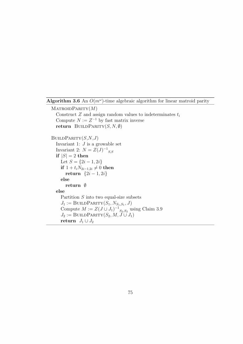
Algorithm 3.6 An O(mω)-time algebraic algorithm for linear matroid parity

MatroidParity(M)Construct Z and assign random values to indeterminates tiCompute N := Z−1 by fast matrix inversereturn BuildParity(S,N, ∅)

BuildParity(S,N ,J)Invariant 1: J is a growable setInvariant 2: N = Z(J)−1S,Sif |S| = 2 then

Let S = 2i− 1, 2iif 1 + tiN2i−1,2i 6= 0 thenreturn 2i− 1, 2i

elsereturn ∅

elsePartition S into two equal-size subsetsJ1 := BuildParity(S1, NS1,S1 , J)Compute M := Z(J ∪ J1)−1S2,S2

using Claim 3.9J2 := BuildParity(S2,M, J ∪ J1)return J1 ∪ J2

75

so the invariant is also satisfied with the second recursive call. Note S is parti-

tioned in such a way that its first half goes to S1 and the remaining goes to S2,

so both S1 and S2 must be parity set.

In the algorithm every element of M is considered. By Claim 3.8, Z(J) is always

non-singular. Hence, by Theorem 3.7, this implies that J is always a growable

set.

Time complexity: In the following claim we show how to compute M :=

Z(J ∪ J1)−1S2,S2efficiently.

Claim 3.9. Let J ′ = J∪J1, J1 ⊆ S. Using N = Z(J)−1S,S, computing Z(J ′)−1S,Scan be done in O(|S|ω) time.

Proof. Since Z(J ′) is identical to Z(J) except Z(J ′)J1,J1 = 0, since Z(J)−1R,C =

NR,C , by Theorem 2.16(3),

Z(J ′)−1S,S = NS,S −NS,J1(I + (−Z(J)J1,J1)NJ1,J1)−1(−Z(J)J1,J1)NJ1,S

= NS,S +NS,J1(I − ZJ1,J1NJ1,J1)−1ZJ1,J1NJ1,S

Note the last equality holds because Z(J)J1,J1 = ZJ1,J1 . At any time during the

computation, matrices involved have size at most |S| × |S|. Hence computing

Z(J ′)−1S,S takes O(|S|ω) time.

Since Z has dimension (2m+ r)× (2m+ r), initial computation of Z−1S,S takes

O((2m + r)ω) = O(mω) time. Let f(m) be the time required by BuildParity

with |S| = 2m, then

f(m) = 2 · f(m/2) +O(mω)

which implies f(n) = O(mω) by the master theorem.

3.6.3 An O(mrω−1) Algorithm

The previous algorithm works for matroids with large rank. In this section we

present an algorithm with better time complexity when rank is small. The idea

76

behind is to break the ground set S into a number of smaller pieces. In this way,

inverse of these matrices to be computed will have smaller size.

Algorithm 3.7 An O(mrω−1)-time algebraic algorithm for linear matroid parity

MatroidParity(M)Construct Z and assign random values to indeterminates tiCompute Y := MT−1MT using Claim 3.10Parition S into m/r subsets each with size rJ := ∅for i = 1 to m/r do

Compute N := Z(J)−1Si,Si using Claim 3.12J ′ := BuildParity(Si, N, J)J := J ∪ J ′

return J

To achieve this we make use of Schur’s formula (Theorem 2.14). Denote Y =

MT−1MT as the Schur complement of T in Z. By Theorem 2.14,

Z−1 =

(Y −1 −Y −1MT−1

T−1MTY −1 T−1 − T−1MTY −1MT−1

)(3.6.3)

We will assume Y −1 exists; otherwise, if Y has no inverse, then we can conclude

that Z has no inverse by Theorem 2.14 and thus there is no parity basis. In

the following we will show how to compute Y efficiently, and then show how to

compute Z(J)−1Si,Si efficiently.

Claim 3.10. Let Y = MT−1MT , Y −1 can be computed in O(mrω−1) time.

Proof. First we show that MT−1R,C can be computed in O(RC) time. Recall

that T is a skew-symmetric matrix, having exactly one entry in each row and

column. Moreover, the positions of the non-zero entries in T are just one row

above or below the diagonal of T . It is thus easy to compute T−1. If Ti,j is

zero, then T−1i,j is also zero. Otherwise T−1i,j = −1/Ti,j. As a result T−1 is

also skew-symmetric and shares the same special structure of T . Therefore any

entry of MT−1 can be computed in O(1) time. Hence MT−1R,C takes O(RC) to

compute.

77

Now we are going to show MT−1MT can be computed in O(mrω−1) time. Since

M has size r ×m, MT−1 can be computed in O(mr) time. To compute product

of MT−1 (size r×m) and MT (size m× r), we can break each of them into m/r

matrices each of size r × r, so computation of their products takes O(mrω−1).

Finally Y is of size r × r and its inverse can be computed in O(rω) time.

Next we show how to compute Z(J)−1Si,Si efficiently using Y −1.

Claim 3.11. Given the matrix Y −1, for any A,B ⊆ S with |A|, |B| ≤ r, Z−1A,B

can be computed in O(rω) time.

Proof. By Equation 3.6.3,

Z−1S,S = T−1 − T−1MTY −1MT−1

Hence for any A,B ⊆ S,

Z−1A,B = T−1A,B − (T−1MT )A,∗Y−1(MT−1)∗,B

Both (T−1MT )A,∗ and (MT−1)∗,B have size r × r and can be computed in O(r2)

time by Claim 3.10. Thus the whole computation takes O(rω) time.

Claim 3.12. In each loop iteration, the matrix Z(J)−1Si,Si can be computed in

O(rω) time.

Proof. Since Z(J) is identical to Z except Z(J)J,J = 0, by using Theorem 2.16(3)

with MSi,Si −MSi,Si = −Z(J)J,J , we have

Z(J)−1Si,Si = Z−1Si,Si + Z−1Si,J(I − ZJ,JZ−1J,J)−1ZJ,JZ−1

J,Si

All the submatrices Z−1Si,Si , Z−1

Si,J , Z−1J,J and Z−1J,Si can be computed in

O(rω) by Claim 3.11. Thus the whole computation can be done in O(rω) time.

Since |Si| = r, each call to BuildParity takes O(rω) time. Hence the overall

time complexity of Algorithm 3.7 is O(m/r · rω) = O(mrω−1).

78

3.7 Maximum Cardinality Matroid Parity

The algorithms in previous sections can only produce a parity basis if one exists.

If there is no parity basis, these algorithms are only be able to report so. In

this section, we present how to find the maximum number of pairs that are

independent. We are going to show an O(rω) time reduction, that reduce a

maximum cardinality matroid parity problem to a problem of computing parity

basis. Hence algorithms in previous sections can be applied.

The idea here is to find a maximum rank submatrix of the matrix formulation

for matroid parity. Such a submatrix is of full rank and corresponds to a new

instance of matroid parity problem which has a parity basis.

Let Y be matrix formulation for the parity problem constructed as in Theo-

rem 2.9. Let r′ be the rank of Y . We first find a maximum rank submatrix YR,C

of Y where |R| = |C| = r′. This can be done in O(rω) time using a variant of the

LUP decomposition algorithm by Harvey (Appendix A of [29]). Since Y is a skew

symmetric matrix, YR,R is also a maximum rank submatrix of Y (Theorem 2.6).

The matrix YR,R can be interpreted as matrix formulation for a new matroid

parity instance. Such an instance contains all the original given pairs, but only

contains rows indexed by R. Then

m∑i=1

xi(biR ∧ ciR) = YR,R,

where biR denotes the vector containing entries of bi index by R. Since YR,R is of

full rank, such a new instance of matroid parity has a parity basis.

The column pairs that are independent in the new instance are also independent

in the original instance. Hence a parity basis of this new instance corresponds to

a parity set of the original instance. In addition, this new instance for matroid

parity can be solved using any algorithm presented.

Since Algorithm 3.7 has time complexity O(mrω−1), we want this reduction to

be done under the same time, but a naive construction of Y would take O(mr2)

time. In the proof of Theorem 2.9, we have shown that the matrix formulation

79

Y is equivalent to another matrix Z in Theorem 2.10. In addition, we have

Y = MT−1MT which can be computed in O(mrω−1) time by Claim 3.10.

3.8 Open Problems

There are some interesting open problems remained. When we solve graphs

problems through matroid parity we rely on the fact that each column has one

or two non-zero entries. A question to ask is whether we can give a more efficient

algorithm if each row has only a few non-zero entries. A positive answer will

imply a faster algorithm for the minimum pinning set problem (Section 2.1.4).

Another problem is the weighted linear matroid parity problem. We have shown a

faster pseudo-polynomial time algorithm with time complexity O(Wmrω). There

is a gap between this and the O(W 1+εmrω−1) algebraic algorithm for linear ma-

troid intersection. Can this gap be closed? Of course the bigger question to ask

is whether there exists a truly polynomial time algorithm for the weighted linear

matroid parity problem.

We gave faster algorithms for some applications of linear matroid parity. But

there remain many important applications of linear matroid parity, for example

the spanning tree packing problem. Can we design algebraic algorithms that are

faster than the best known combinatorial algorithms?

80

Chapter 4

Graph Connectivities

The results presented in this chapter are based on joint work with Lap Chi Lau

and Kai Man Leung [12].

4.1 Introduction

Graph connectivity is a basic concept that measures the reliability and efficiency

of a graph. The edge connectivity from vertex s to vertex t is defined as the size

of a minimum s-t cut, or equivalently the maximum number of edge disjoint paths

from s to t. Computing edge connectivities is a classical and well-studied problem

in combinatorial optimization. Most known algorithms to solve this problem are

based on network flow techniques (see e.g. [63]).

The fastest algorithm to compute s-t edge connectivity in a simple directed graph

runs in O(minm1/2, n2/3·m) time by Even and Tarjan [19], where m is the num-

ber of edges and n is the number of vertices. To compute the edge connectivities

for many pairs, however, it is not known how to do it faster than computing edge

connectivity for each pair separately, even when the pairs share the source or the

sink. For instance, it is not known how to compute all pairs edge connectivities

faster than computing s-t edge connectivity for Ω(n2) pairs. This is in contrast

to the problem in undirected graphs, where all pairs edge connectivities can be

computed in O(mn) time by constructing a Gomory-Hu tree [4].

81

In this chapter we study edge connectivities in simple directed planar graphs and

its generalizations. In a recent work, we give a new algebraic formulation to

the edge connectivities problem using network coding [12]. Construct an m×mmatrix K as follows, if the head of ei is equal to the tail of ej then we set Ki,j = ki,j

where ki,j is a distinct indeterminate, 0 otherwise. Earlier in Theorem 2.26 we

have shown the matrix has the following properties:

Theorem 2.26. The s-t edge connectivity is equal to the rank of the submatrix

(I −K)−1δout(s),δin(t). In addition, if we substitute indeterminates ki,j with random

values from a field F, then the claim still holds with probability 1−O(m3/|F|).

This formulation allows us to compute edge connectivities between many vertex

pairs simultaneously. It implies an O(mω) time algorithm for all pairs edge con-

nectivities in general graphs as shown in Section 2.5. Thus it implies an O(nω)

time algorithm for planar graphs, bounded genus graphs and fixed minor free

graphs, since these graphs have O(n) edges [45, 68]. This is an improvement over

the current algorithms, as the edge connectivity of one pair in a simple directed

planar graphs takes O(n) time [6] to compute.

The bottleneck of the O(mω) time algorithm is the step to compute (I −K)−1.

Thus we are motivated to study in what situation can we compute (I − K)−1

more efficiently. One approach to compute the inverse of a matrix is to apply

Schur’s formula (Theorem 2.14). Recall the theorem,

Theorem 2.14. Let

M =

(A B

C D

),

where A and D are square matrices and denote S = D − CA−1B. If A is non-

singular then det(M) = det(A)×det(S). Furthermore if A and S are non-singular

then

M−1 =

(A−1 + A−1BS−1CA−1 −A−1BS−1

−S−1CA−1 S−1

).

Our observation is that for graphs with good separators, we can find a partition

of (I−K) such that B and C are of low rank, so that we can compute (I−K)−1

faster by a divide and conquer algorithm.

82

Using the observation, we come up with a randomized algorithm that compute the

edge connectivities between all pairs of vertices in O(dω−2nω/2+1) time for simple

directed fixed minor free graphs with maximum degree d. This implies that we

can compute the edge connectivity between one pair of vertices in amortized

O(d0.4n0.2) time. This method is an improvement over the O(nω) time algorithm

when d = O(√n).

The rest of this chapter is organized as follows. In Section 4.2, we will show that

if a matrix is “well-separable” (to be defined in the next section), then its inverse

can be computed more efficiently. Then in Section 4.3, we show that the matrix

I −K for fixed minor free graphs is well-separable, and conclude that the edge

connectivities in such graphs can be computed efficiently.

4.2 Inverse of Well-Separable Matrix

We say an n× n matrix M is (r, α)-well-separable (α is a constant smaller than

one) if M is invertible and it can be written as

M =

(A B

C D

)

so that both A and D are (r, α)-well-separable square matrix with dimension no

more than αn, and also both B and C are of rank no more than r. In this section

we are going to show that the inverse of a well-separable matrix can be computed

in O(rω−2n2) time.

To compute M−1, we first compute the inverses of A and D recursively. We

will compute M−1 using Schur’s formula. A key step is to use the Sherman-

Morrison-Woodbury formula (Theorem 2.15) to compute S−1 efficiently, instead

of computing D − CA−1B and then (D − CA−1B)−1.

Firstly, since rank(B), rank(C) ≤ r, we can write B = BuBTv and C = CuC

Tv

where Bu, Bv, Cu and Cv are size O(n) × r matrices. This can be done in

O(rω−2n2) time by Theorem 2.13.

83

Claim 4.1. If we have A−1 and D−1, then we can compute S−1 = (D−CA−1B)−1

in O(rω−2n2) time.

Proof. By Schur’s formula (Theorem 2.14) S = D−CA−1B is non-singular if M−1

and A−1 exist. The proof consists of two steps. We will first write CA−1B as a

product of two low rank matrices. Then we use the Sherman-Morrison-Woodbury

formula to compute S−1 efficiently. In the following, rectangular matrix multi-

plications will be done by dividing each matrix into submatrices of size r × r.

Multiplications between these submatrices can be done in O(rω) time.

First we consider CA−1B, which is equal to (CA−1Bu)BTv . C(A−1Bu) is of size

O(n)×r and can be computed using O(n2/r2) submatrices multiplications of size

r × r. By putting U = CA−1Bu and V = Bv, we have CA−1B = UV T where U

and V are of size O(n)× r.

Now we can use Theorem 2.15 (Sherman-Morrison-Woodbury formula) to com-

pute (D+UV T )−1 efficiently since D−1 is known and U , V are low rank matrices.

By the formula,

S−1 = D−1 −D−1U(I + V TD−1U)−1V TD−1.

Similar to the above V TD−1U can be computed using O(n2/r2) submatrix multi-

plications. Since S is non-singular, (I+V TD−1U)−1 exists by Theorem 2.15, and

it can be computed in one submatrix multiplication time as I+V TD−1U is of size

r × r. Finally, since (D−1U)T and (V TD−1) are r ×O(n) matrices, we can com-

pute (D−1U)(I+V TD−1U)−1(V TD−1) using O(n2/r2) submatrix multiplications.

Hence the overall time complexity is O(rω × n2/r2) = O(rω−2n2).

Using Claim 4.1, we can now compute M−1 using Schur’s formula efficiently.

Claim 4.2. If we have A−1, D−1 and S−1, then we can compute M−1 in O(rω−2n2)

time.

Proof. By Schur’s formula, to compute M−1, we need to compute A−1BS−1CA−1,

A−1BS−1 and S−1CA−1. These multiplications all involve some O(n)× r matrix

Bu, Bv, Cu or Cv follows:

84

• A−1BS−1CA−1 = (A−1Bu)(BTv S−1CA−1)

• A−1BS−1 = (A−1Bu)(BTv S−1)

• S−1CA−1 = (S−1Cu)(CTv A−1)

All steps during computation of these products involve an O(n)× r (or r×O(n))

matrix, thus we can avoid computing the product of two n× n matrices. Hence

they all only take O(n2/r2) submatrix multiplications to compute. Therefore the

total time complexity is O(rω × n2/r2) = O(rω−2n2).

By Claim 4.1 and Claim 4.2, we can compute M−1 in O(rω−2n2) time if we are

given A−1, D−1 and also low rank decomposition of B and C. We can then use

a recursive algorithm to compute M−1.

Theorem 4.3. If an n× n matrix M is (r, α)-well-separable, and the separation

can be found in O(nγ) time, then M−1 can be computed in O(nγ + rω−2n2) time.

Proof. First we analyse the time to compute M−1. We use a O(nγ) time algorithm

to find an (r, α)-well-separable partition of M . By the property of the partition,

both B and C are matrices of rank at most r. Then we can write B = BuBTv and

C = CuCTv in O(rω−2n2) time where Bu, Bv, Cu and Cv are all O(n)× r matrices

by Theorem 2.13. We then compute A−1 and D−1 recursively, as A and D by

definition are also (r, α)-separable. Using these inverses we can apply Claim 4.1

to compute S−1, then apply Claim 4.2 to compute M−1 using A−1, D−1 and S−1.

Thus, given A−1 and D−1, we can compute M−1 in O(rω−2n2) time. Let f(n) be

the time to compute M−1 of size n× n. Then

f(n) = f(αn) + f((1− α)n) +O(nγ) +O(rω−2n2),

and it remains to show f(n) = O(nγ + rω−2n2).

For simplicity, we prove the case that nγ is dominated by rω−2n2, which is the

case that will happen in the next section. The another case follows with a very

similar analysis. Let f(n) = f(αn) + f((1−α)n) + krω−2n2 for some constant k,

85

We will show f(n) ≤ crω−2n2 for some large enough constant c using induction.

f(n) = crω−2(αn)2 + crω−2((1− α)n)2 + krω−2n2

= (cα2 + c(1− α)2 + k)rω−2n2

≤ crω−2n2

4.3 Directed Graphs with Good Separators

In this section we show that all pairs edge connectivities in planar graphs, bounded

genus graphs, and fixed minor free graphs can be computed in O(dω−2nω/2+1)

time.

We will first see that the underlining matrix I − K for these graphs are well

separable. Thus we can apply Theorem 4.3 together with the fact the these

graphs have O(n) edges, to obtain a O(dω−2nω/2+1) time algorithm to compute

(I −K)−1. Finally we can apply Theorem 2.26, and then show that the time to

compute the required ranks of all submatrices in (I −K)−1 is O(dω−2nω/2+1).

We say an undirected graph G = (V,E) has a (f(n), α)-separation, if V can be

partitioned into three parts, X, Y, Z such that |X ∪ Z| ≤ α|V |, |Y ∪ Z| ≤ α|V |,|Z| ≤ f(n), and there is no edge between X and Y . Planar graphs, bounded

genus graphs and fixed minor free graphs all have (O(√n), 2/3)-separation which

can be found in O(n1.5) time [1]. In addition, these graphs are closed under taking

subgraphs. So we can recursively separate the separated parts X and Y until the

separated pieces are small enough.

For a graph G (and its subgraph) that has O(n) edges and a (O(√n), 2/3)-

separation, we claim that the matrix I − K of G is (O(d√n, α)-well-separable

for some constant α < 1. Recall that an n× n matrix is (f(n), α)-well-separable

if we can partition the matrix so that submatrices A and D are square matrices

having dimension ≤ αn and are also (f(n), α)-well-separable, while submatrices

B and D are of rank at most f(n).

86

To show that I − K is well-separable, we prove by induction on the number of

edges of the graph. We will first show the inductive step and then by the base

case. For the inductive step, we can use a separator to divide the graph into three

parts X, Y, Z such that |X ∪ Z| ≤ 2n/3, |Y ∪ Z| ≤ 2n/3 and |Z| = O(√n), and

there are no edges between X and Y . Let E1 be the set of edges with at least

one endpoint in X and let E2 be E − E1. We partition I −K as follows.

(E1 E2

E1 A B

E2 C D

)

Since |Y | = Ω(n) and each vertex in Y is of degree at least 1, we have |E1| = Ω(n)

and |E2| = Ω(n). Also we have |E1| = O(n) and |E2| = O(n) since m = O(n),

and thus |E1|, |E2| ≤ αn for some constant α. Let F1 be the subset of E1 with

one endpoint in Z, and define F2 similarly. Then any edge in E1 − F1 does

not share an endpoint with any edge in E2 − F2. Since |Z| = O(√n) and each

vertex is of degree at most d, there are at most O(d√n) edges with one endpoint

in Z, and thus |F1| = O(d√n) and |F2| = O(d

√n). Therefore, submatrices B

and C have O(d√n) non-zero rows and columns, and thus are of rank at most

O(d√n). Also I −K must be invertible because I −K has ones on its diagonal,

and thus det(I −K) is a non-zero polynomial. Matrices A and D correspond to

matrices I −K for subgraphs of G, and by the inductive hypothesis A and D are

(O(d√n), α)-well-separable. Hence we can conclude that I −K is (O(d

√n), α)-

well-separable.

For the base case of the induction, observe that any small enough graph must be

separable. For any graph with the number of edges less than a small constant c,

we can safely assume its matrix I−K is (O(d√n), α)-well-separable because any

way to partition the edge set into halves gives B and C rank less than c.

Now it remains to analyze the probability that all I − K, A and D remain

invertible after substituting random values to ki,j. Note that det(I − K) is a

degree m polynomial not identically equal to zero, because I − K has ones on

its diagonal. Thus, by the Schwartz-Zippel Lemma, I − K is invertible with

probability at least 1−m/|F|. Since A and D correspond to matrices I −K for

87

subgraphs of G, we can apply the same argument to A and D recursively, and all

the required matrices are invertible with probability at least 1−O(m logm)/|F|.

As a result I −K is (O(d√n), α)-well-separable. We can now apply Theorem 4.3

with γ = 1.5 [1]. So (I − K)−1 can be computed in O(n1.5 + (d√n)ω−2n2) =

O(dω−2nω/2+1) time.

Finally we analyze the required time to compute the rank of (I −K)−1δout(s),δin(t)for all source s and sink t. We will show that this can be done in O(dω−2n2) time.

Since the rank of an a × b matrix can be computed in O(abω−1) time by Theo-

rem 2.12. The ranks of (I −K)−1δout(s),δin(t) from one source s to all receivers t

can be computed in∑t∈v

O(din(t) · (dout(s))ω−1) = O(m · (dout(s))ω−1)

time. So the overall time to compute the ranks for all pairs of vertices is∑s∈v

O(n · (dout(s))ω−1)

as m = O(n). Now we show that this sum is at most O(dω−2n2). Let di = dout(vi).

We partition the vertices into into groups Vj so that∑

i∈Vj di ≤ d, where d is the

maximum degree of the graph. Note that there exists a partition so that all Vj

(except at most one) has

d/2 ≤∑i∈Vj

di ≤ d,

otherwise we can merge two groups that has sum less then d/2. Thus there are

at most m/(d/2) + 1 = O(n/d) groups. Now we can bound the overall time to

compute the ranks,∑s∈v

∑t∈v

din(t) · (din(s))ω−1 = n ·∑s∈v

(din(s))ω−1

= n ·O(n/d)∑j=1

∑s∈Vj

(din(s))ω−1

88

≤ n ·O(n/d)∑j=1

∑s∈Vj

din(s)

ω−1

≤ n ·O(n/d)∑j=1

dω−1

= n ·O(n/d) · dω−1

= O(dω−2n2).

The first inequality is true because din(s) are all positive and the exponent ω− 1

is not smaller than one. Hence the total time to compute the ranks is O(dω−2n2),

which is dominated by the time to compute (I−K)−1. And we have the following

conclusion.

Corollary 4.4. All pairs edge connectivities can be computed in O(dω−2nω/2+1)

time for any directed fixed minor free graph with maximum degree d.

4.4 Open Problems

After the discussion on the algebraic approach on the graph connectivity problem

in this chapter, there are some interesting problems remain. Is it possible to give

an O(nω) time algorithm to compute the edge connectivity between one pair

of vertices? If such algorithm exists then we can also compute all pairs edge

connectivities in O(nω+2) time, which is faster than the O(mω) time algorithm

we discussed.

Can we drop the requirement that the maximum degree d of the given graph

is small for our all pairs edge connectivities algorithm for planar graphs and its

generalization? On other hand, can this algebraic approach be generalized to the

capacitated case, where each edge has a capacity?

Finally, is it possible to design a combinatorial algorithm, that is faster than

computing the edge connectivities between each pair of vertices separately in

directed graphs?

89

90

Bibliography

[1] N. Alon, P. Seymour, and R. Thomas. A separator theorem for nonplanargraphs. Journal of the American Mathematical Society, 3(4):801–808, 1990.

[2] M.A. Babenko. A fast algorithm for the path 2-packing problem. Theory ofComputing Systems, 46(1):59–79, 2010.

[3] P. Berman, M. Furer, and A. Zelikovsky. Applications of the linear matroidparity algorithm to approximating steiner trees. In Proceedings of the 1stInternational Computer Science Symposium in Russia (CSR), pages 70–79,2006.

[4] A. Bhalgat, R. Hariharan, T. Kavitha, and D. Panigrahi. An O(mn) Gomory-Hu tree construction algorithm for unweighted graphs. In Proceedings of the39th ACM Symposium on Theory of Computing (STOC), pages 605–614,2007.

[5] A. Bouchet and W.H. Cunningham. Delta-matroids, jump systems, andbisubmodular polyhedra. SIAM Journal on Discrete Mathematics, 8(1):17–32, 1995.

[6] U. Brandes and D. Wagner. A linear time algorithm for the arc disjointMenger problem in planar directed graphs. Algorithmica, 28:16–36, 2000.

[7] J.R. Bunch and J.E. Hopcroft. Triangular factorization and inversion by fastmatrix multiplication. Mathematics of Computation, 28(125):231–236, 1974.

[8] G. Calinescu, C.G. Fernandes, U. Finkler, and H. Karloff. A better ap-proximation algorithm for finding planar subgraphs. Journal of Algorithms,27(2):269–302, 1998.

[9] P.M. Camerini, G. Galbiati, and F. Maffioli. Random pseudo-polynomialalgorithms for exact matroid problems. Journal of Algorithms, 13(2):258–273, 1992.

91

[10] P. Chalasani and R. Motwani. Approximating capacitated routing and de-livery problems. SIAM Journal on Computing, 28:2133–2149, 1999.

[11] H.Y. Cheung, L.C. Lau, and K.M. Leung. Algebraic algorithms for linearmatroid parity problems. In Proceedings of the 22nd ACM-SIAM Symposiumon Discrete algorithms (SODA), pages 1366–1382, 2011.

[12] H.Y. Cheung, L.C. Lau, and K.M. Leung. Graph connectivities, networkcoding, and expander graphs. Manuscript, 2011.

[13] M. Chudnovsky, W.H. Cunningham, and J. Geelen. An algorithm for packingnon-zero A-paths in group-labelled graphs. Combinatorica, 28(2):145–161,2008.

[14] D. Coppersmith and S. Winograd. Matrix multiplication via arithmetic pro-gressions. Journal of Symbolic Computation, 9(3):251–280, 1990.

[15] T.H. Cormen, C.E. Leiserson, R.L. Rivest, and C. Stein. Introduction toalgorithms. MIT Press, 2001.

[16] W.H. Cunningham and J.F. Geelen. The optimal path-matching problem.Combinatorica, 17(3):315–337, 1997.

[17] J. Edmonds. Submodular functions, matroids, and certain polyhedra. InCalgary International Conference on Combinatorial Structures and TheirApplications, pages 69–87, 1970.

[18] J. Edmonds. Matroid intersection. Annals of Discrete Mathematics, 4:39–49,1979.

[19] S. Even and R.E. Tarjan. Network flow and testing graph connectivity. SIAMJournal on Computing, 4(4):507–518, 1975.

[20] M.L. Furst, J.L. Gross, and L.A. McGeoch. Finding a maximum-genus graphimbedding. Journal of the ACM, 35(3):523–534, 1988.

[21] H.N. Gabow. A matroid approach to finding edge connectivity and packingarborescences. Journal of Computer and System Sciences, 50(2):259–273,1995.

[22] H.N. Gabow and M. Stallmann. Efficient algorithms for graphic matroidintersection and parity. In Proceedings of the 12th International Colloquiumon Automata, Languages and Programming (ICALP), pages 210–220, 1985.

92

[23] H.N. Gabow and M. Stallmann. An augmenting path algorithm for linearmatroid parity. Combinatorica, 6(2):123–150, 1986.

[24] H.N. Gabow and Y. Xu. Efficient algorithms for independent assignment ongraphic and linear matroids. In Proceedings of the 30th Annual Symposiumon Foundations of Computer Science (FOCS), pages 106–111, 1989.

[25] J. Geelen and S. Iwata. Matroid matching via mixed skew-symmetric ma-trices. Combinatorica, 25(2):187–215, 2005.

[26] C.D. Godsil. Algebraic combinatorics. Chapman & Hall mathematics. Chap-man & Hall, 1993.

[27] M.X. Goemans. Minimum bounded degree spanning trees. In Proceedingsof the 47th Annual IEEE Symposium on Foundations of Computer Science(FOCS), pages 273–282, 2006.

[28] N.J.A. Harvey. An algebraic algorithm for weighted linear matroid intersec-tion. In Proceedings of the 18th ACM-SIAM Symposium on Discrete algo-rithms (SODA), pages 444–453, 2007.

[29] N.J.A. Harvey. Matchings, Matroids and Submodular Functions. PhD thesis,Massachusetts Institute of Technology, 2008.

[30] N.J.A. Harvey. Algebraic algorithms for matching and matroid problems.SIAM Journal on Computing, 39(2):679–702, 2009.

[31] N.J.A. Harvey, D.R. Karger, and K. Murota. Deterministic network codingby matrix completion. In Proceedings of the 16th ACM-SIAM Symposiumon Discrete algorithms (SODA), pages 489–498, 2005.

[32] R. Hassin and A. Levin. An efficient polynomial time approximation schemefor the constrained minimum spanning tree problem using matroid intersec-tion. SIAM Journal of Computing, 33:261–268, 2004.

[33] R.A. Horn and C.R. Johnson. Matrix analysis. Cambridge University Press,1990.

[34] T.A. Jenkyns. Matchoids: a generalization of matchings and matroids. PhDthesis, University of Waterloo, 1974.

[35] P.M. Jensen and B. Korte. Complexity of matroid property algorithms.SIAM Journal on Computing, 11:184–190, 1982.

93

[36] T. Jordan. Rigid and globally rigid graphs with pinned vertices. In Fete ofCombinatorics and Computer Science, pages 151–172, 2010.

[37] E. Kaltofen and V. Pan. Processor efficient parallel solution of linear systemsover an abstract field. In Proceedings of the 3rd ACM Symposium on ParallelAlgorithms and Architectures, pages 180–191, 1991.

[38] S. Khuller and U. Vishkin. Biconnectivity approximations and graph carv-ings. Journal of the ACM, 41:214–235, 1994.

[39] E.L. Lawler. Combinatorial optimization: networks and matroids. OxfordUniversity Press, 1976.

[40] J. Lee, M. Sviridenko, and J. Vondrak. Matroid matching: the power of localsearch. In Proceedings of the 42nd ACM Symposium on Theory of Computing(STOC), pages 369–378, 2010.

[41] L. Lovasz. On determinants, matchings and random algorithms. Fundamen-tals of Computation Theory, 79:565–574, 1979.

[42] L. Lovasz. Matroid matching and some applications. Journal of Combina-torial Theory, Series B, 28(2):208–236, 1980.

[43] L. Lovasz. The membership problem in jump systems. Journal of Combina-torial Theory, Series B, 70(1):45–66, 1997.

[44] L. Lovasz and M.D. Plummer. Matching theory. Elsevier, 1986.

[45] W. Mader. Homomorphiesatze fur graphen. Mathematische Annalen,178:154–168, 1968.

[46] W. Mader. Uber die maximalzahl kreuzungsfreier H-Wege. Archiv der Math-ematik, 31(1):387–402, 1978.

[47] R. Motwani and P. Raghavan. Randomized algorithms. Cambridge UniversityPress, 1995.

[48] M. Mucha and P. Sankowski. Maximum Matchings via Gaussian Elimina-tion. In Proceedings of the 45th Annual IEEE Symposium on Foundationsof Computer Science (FOCS), pages 248–255, 2004.

[49] M. Mucha and P. Sankowski. Maximum matchings in planar graphs viaGaussian elimination. Algorithmica, 45:3–20, 2006.

94

[50] K. Mulmuley, U.V. Vazirani, and V.V. Vazirani. Matching is as easy asmatrix inversion. In Proceedings of the 19th ACM Symposium on Theory ofComputing (STOC), pages 345–354, 1987.

[51] K. Murota. Matrices and matroids for systems analysis. Springer Verlag,2009.

[52] H. Narayanan, H. Saran, and V.V. Vazirani. Randomized parallel algorithmsfor matroid union and intersection, with applications to arborescences andedge-disjoint spanning trees. SIAM Journal on Computing, 23(2):387–397,1994.

[53] C.St.J.A Nash-Williams. Connected detachments of graphs and generalizedEuler trails. Journal of the London Mathematical Society, 2(1):17–29, 1985.

[54] J.B. Orlin. A fast, simpler algorithm for the matroid parity problem. InProceedings of the 13th International Conference on Integer Programmingand Combinatorial Optimization (IPCO), pages 240–258, 2008.

[55] J.B. Orlin and J.H. Vande Vate. Solving the linear matroid parity problemas a sequence of matroid intersection problems. Mathematical Programming:Series A and B, 47(1):81–106, 1990.

[56] G. Pap. Packing non-returning A-paths. Combinatorica, 27(2):247–251,2007.

[57] G. Pap. Some new results on node-capacitated packing of A-paths. InProceedings of the 39th ACM Symposium on Theory of Computing (STOC),pages 599–604, 2007.

[58] G. Pap. Packing non-returning A-paths algorithmically. Discrete Mathemat-ics, 308(8):1472–1488, 2008.

[59] H.J. Promel and A. Steger. A new approximation algorithm for the Steinertree problem with performance ratio 5/3. Journal of Algorithms, 36(1):89 –101, 2000.

[60] M.O. Rabin and V.V. Vazirani. Maximum matchings in general graphsthrough randomization. Journal of Algorithms, 10(4):557–567, 1989.

[61] P. Sankowski. Weighted bipartite matching in matrix multiplication time. InProceedings of the 33rd International Colloquium on Automata, Languagesand Programming (ICALP), pages 274–285, 2006.

95

[62] P. Sankowski. Processor efficient parallel matching. Theory of ComputingSystems, 42:73–90, 2008.

[63] A. Schrijver. Combinatorial optimization: polyhedra and efficiency. SpringerVerlag, 2003.

[64] A. Sebo and L. Szego. The path-packing structure of graphs. In Proceedingsof the 10th Conference on Integer Programming and Combinatorial Opti-mization (IPCO), pages 131–143, 2004.

[65] A. Storjohann. High-order lifting and integrality certification. Journal ofSymbolic Computation, 36(3-4):613–648, 2003.

[66] Z. Szigeti. On a min-max theorem of cacti. In Proceedings of the 6th Con-ference on Integer Programming and Combinatorial Optimization (IPCO),pages 84–95, 1998.

[67] Z. Szigeti. On the graphic matroid parity problem. Journal of CombinatorialTheory, Series B, 88(2):247–260, 2003.

[68] A. Thomason. An extremal function for contractions of graphs. MathematicalProceedings of the Cambridge Philosophical Society, 95:261–265, 1983.

[69] W.T. Tutte. The factorization of linear graphs. Journal of the LondonMathematical Society, 1(2):107, 1947.

[70] M.A. Woodbury. Inverting modified matrices. Memorandum Report, 42:106,1950.

[71] F. Zhang. The Schur complement and its applications. Springer Verlag, 2005.

96