Alessandro Birolini Reliability Engineering · Prof. Dr. Alessandro Birolini ∗ Ponte Vecchio –...

Alessandro Birolini

Reliability Engineering

Alessandro Birolini

ReliabilityEngineeringTheory and Practice

Fifth edition

With 140 Figures, 60 Tables,120 Examples, and 50 Problems

123

Prof. Dr. Alessandro Birolini∗

Ponte Vecchio – Torre degli AmideiI-50122 FirenzeTuscany, Italy

email: [email protected]

∗Ingenieur et penseur, Ph.D., Professor Emeritus of Reliability Engineeringat the Swiss Federal Institute of Technology (ETH), Zürichbiography on: www.ethz.ch/people/whoiswho

Library of Congress Control Number: 2007921004

First and second edition printed under the title “Quality and Reliability ofTechnical Systems”

ISBN 978-3-540-49388-4 5th ed. Springer Berlin Heidelberg New YorkISBN-10 3-540-40287-X 4th ed. Springer Berlin Heidelberg New York

This work is subject to copyright. All rights are reserved, whether the whole or part of the materialis concerned, specifically the rights of translation, reprinting, reuse of illustrations, recitation, broad-casting, reproduction on microfilm or in any other way, and storage in data banks. Duplication ofthis publication or parts thereof is permitted only under the provisions of the German Copyright Lawof September 9, 1965, in its current version, and permission for use must always be obtained fromSpringer. Violations are liable for prosecution under the German Copyright Law.

Springer is a part of Springer Science+Business Media

springer.com

© Springer-Verlag Berlin Heidelberg 1994, 1997, 1999, 2004, and 2007

The use of general descriptive names, registered names, trademarks, etc. in this publication does notimply, even in the absence of a specific statement, that such names are exempt from the relevantprotective laws and regulations and therefore free for general use.

Typesetting: Camera ready by authorProduction: LE-TEX Jelonek, Schmidt & Vöckler GbR, LeipzigCover-Design: medio Technologies AG

Printed on acid-free paper 62/3100/YL - 5 4 3 2 1 0

"La chance vient d l'esprit qui estpr2t d la recevoir. " I )

Louis Pasteur

"Quand on apercoit combien la somme de nos

ignorantes dipasse celle de nos connaissances,

on se serztpeu porti d conclure trop vite. " ZJ

Louis De Broglie

"One has to learn to consider causes rather than

symptoms of undesirable events and avoid hypo-

critical attitudes. " A. B.

'1 "Opportunity Comes to the intellect which is ready to receive it."

2, "When one recognizes how much the sum of our ignorante exceeds that of our knowledge, one is less ready to draw rapid conclusions."

Preface to the 5th Edition

This 5th edition differs from the 4th one for some refinements and extensions mainly on investigation and test of complex repairable systems. For phased-mission systems a new approach is given for both reliability and availability (Section 6.8.6.2). Effects of common cause failures (CCF) are carefully investigated for a 1-out-of-2 redundancy (6.8.7). Petri nets and dynamic FTA are introduced as alternative investigation methods for repairable systems (6.9). Approximate expressions are further developed. An unified approach for availability estimation und demonstration is given for exponentially and Erlangian distributed failure-free and repair times (7.2.2, A8.2.2.4, A8.3.1.4). Con$dence limits at system level are given for the case of constant failure rates (7.2.3.1). Investigation of nonhomogeneous Poisson processes is refined and more general point processes (superimposed, cumulative) are discussed (A7.8), with application to data analysis (7.6.2) & cost optimization (4.7). Trend tests to detect early failures or wearozdi are introduced (7.6.3). A simple demonstration for mean & variance in a cumulative process is given (A7.8.4). Expansion of a redundancy 2-out-of-3 to a redundancy 1-out-of-3 is discussed (2.2.6.5). Some present production-related reliability problems in VLSI ICs are shown (3.3.4). Maintenance strategies are reviewed (4.6).

As in the previous editions of this book, reliability figures at system level have indices SI (e.g. M W i ) , where S stands for system and i is the state entered at t=O (Table 6.2). Furthermore, considering that for a repairable system, operating times between system failures can be neither identically distributed nor independent, failure rate is confined to nonrepairable systems or to repairable systems which are as-good-as-new after repair. Failure intensio is used for general repairable systems. For the cases in which renewal is assumed to occur, the variable X starting by X = 0 at euch renewal is used instead of t, as for interarrival times. Also because of the estimate M ~ B F = T l k , often used in practical applications, MTBF is confined to repairable systems whose failure occurrence can be described by a homogeneous Poisson processes, for which (and only for which) interarrival times are independent exponentially distributed random variables with the same Parameter hs and mean MTBF, = 11 hs (p. 358). For Markov and semi- Markov models, MUTs is used (pp. 265,477). Repair is used as a synonym for restoration, with the assumption that repaired elements in a system are as-good-as-new after repair (the system is as-good-as-new, with respect to the state considered, only if all nonrepaired elements have constant failure rate). Reliability growth has been transferred in Chapter 7 and Table 3.2 on electronic components has been put in the new Appendix A.lO. A set of problems for home- work assignment has been added in the new Appendix A. 11.

This edition extends and replaces the previous editions. The comments of many friends and the agreeable cooperation with Springer-Verlag are gratefully acknowledged.

Zurich and Florence, September 13,2006 Alessandro Birolini

Preface to the 4th Edition The large interest granted to this book made a 4th edition necessary. The structure of the book is unchanged, with its main part in Chapters 1 - 8 and self contained appendices A l -A5 on management aspects and A6 - A8 on basic probability theory, stochastic processes & statistics.

Such a structure allows rapid access to practical results and a comprehensive introduction to the mathematical foundation of reliability theory. The content has been extended and reviewed. New models & considerations have been added to Appendix A7 for stochastic processes (NHPP), Chapter 4 for spare parts provisioning, Chapter 6 for complex repairable systems (imperfect switching, incomplete coverage, items with more than two states, phased-mission systems, fault tolerant reconfigurable systems wi th reward and frequency I duration aspects, Monte Carlo simulation), and Chapters 7 & 8 for reliabilig data analysis. Some results come from a stay in 2001 as Visiting Fellow at the Institute ofAdvanced Study of the University of Bologna.

Performance, dependability, cost, and time to market are key factors for today's products and services. However, failure of complex systems can have major safety consequences. Also here, one has to learn to consider causes rather than syrnptoms o f undesirable events und avoid hypocritical attitudes. Reliability engineering can help. Its purpose is to develop methods und tools to evaluate und demonstrate reliability, maintainability, availability, and safety of components, equipment & systems, and to support development and production engineers in building in these characteristics. To build in reliability, maintainability, and safety into complex systems, failure rate and failure mode analyses must be performed early in the development phase and be supported (as far as possible) by failure mechanism analysis, design guidelines, and design reviews. Before production, qual$cation tests are necessary to venfy that targets have been achieved. In the production phase, processes have to be qualified and monitored to assure the required quality level. For many systems,availability requirements have to be met and stochastic processes are used to investigate and optimize reliability and availability, including logistic support as well. Software often plays a dominant role, requiring specific quality assurance activities. Finally, to be cost and time effective, reliability engineering has to be coordinated with quality management (TQM) efforts, including value engineering and concurrent engineering, as appropriate.

This book presents the state-of-the-art of reliability engineering in theory and practice. It is a textbook based on the author's experience of 30 years in this field, half in industry and as founder of the Swiss Test Lab. for VLSI ICs in Neuchatel, and half as Professor (full since 1992) of Reliability Engineering at the Swiss Federal Institute of Technology (ETH), Zurich. It also reflects the experience gained in an effective cooperation between University and industry over 10 years with more than 30 medium and large industries [1.2 (1996)]+). Following Chapter 1, the book is structured in three p a r k

1. Chapters 2 - 8 deal with reliability, maintainability, and availability analysis und test, with emphasis on practical aspects in Chapters 3, 5, and 8. This part answers the question of how to build in, evaluate, und dernonstrate reliability, maintainability, und availability.

2. Appendices A l - A5 deal with definitions, standards, and program plans for quality and reliability assurancel management of complex systems. This minor part of the book has been added to comment on definitions and standards, and to support managers in answering the question of how to specify und achieve high reliability targets for complex Systems, when tailon'ng is not rnandatory.

3. Appendices A6 - A8 give a comprehensive introduction to probability theory, stochastic processes, and statistics, as needed in Chapters 2, 6, and 7, respectively. Markov, semi- Markov, and semi-regenerative processes are introduced with a view developed by the author in [A7.2 (1975 & 1985)l. Tkispart is addressed to systern oriented engineers.

Methods and tools are presented in a way that they can be tailored to Cover different levels of reliability requirements (the reader has to select this level). Investigation of repairable systems is performed systematically for many of the structures occurring in practical applications,

starting with constant failure and repair rates and generalizing step by step up to the case in which the process involved is regenerative with a minimum number o f regeneration states. Considering for each element M7TR (mean time to repair) << M V F (mean time to failure), it is shown that the shape of the repair time distribution has a small influence on the results at system level and, for constant failure rate, the reliability function at the system level can often be approximated by an exponential function. For large series - parallel systems, approximate expressions for reliability and availability are developed in depth, in particular using macro structures as introduced by the author in [6.5 (1991)l. Procedures to investigate repairable Systems with complex structure (for which a reliability block diagram often does not exist) are given as further application of the tools introduced in Appendix A7, in particular for imperfect switching, incomplete fault coverage, elements with more than two states, phased-mission systems, and fault tolerant reconfigurable systems with reward & frequency I duration aspects. New design d e s have been added for imperfect switching and incomplete coverage. A Monte Carlo approach useful for rare events is given. Spare parts provisioning is discussed for decentralized and centralized logistic support. Estimation and demonstration of a constant failure rate and statistical evaluation of general reliability data are considered in depth. Qualification tests and screening for components and assemblies are discnssed in detail. Methods for causes-to-effects analysis, design guidelines for reliability, maintainability & software quality, and checklists for design reviews are considered carefully. Cost optimization is investigated for some practical applications. Standards and trends in quality management are discussed. A large number of tables, figures, and examples support practical aspects

It is emphasized that care is necessary in the statistical analysis of reliability data (in particular for accelerated tests and reliability growth), causes-to-effects analysis should be performed systematically at least wkere redundancy appears (also to support remote maintenance), and further efforts should be done for developing approximate expressions for complex repairable systems as well as models for fault tolerant systems with hardware und software.

Most of the methods & tools given in this book can be used to investigatelimprove safety as well, which no longer has to be considered separately from reliability (although modeling human aspects can lead to some difficulties). The Same is forprocess and sewices reliability.

The book has been used for many years (Ist German Ed. 1985, Springer) as a textbook for three Semesters beginning graduate students at the ETH Zurich and for Courses aimed at engineers in industry. The basic Course (Chapters 1, 2, 5 & 7, with introduction to Chapters 3,4, 6 & 8) should belong to the curriculum of most engineering degrees.

This edition extends and reviews the 3rd Edition (1999). It aims further to establish a link between theory und practice, to be a contribution to a continuous learning program und a sustainable development, und to support creativity (stimulated by an internal confidence and a deep observation of nature, but restrained by excessive bureaucracy or depersonalization). The comments of many friends and the agreeable cooperation with Springer-Verlag are gratefully acknowledged.

Zurich and Florence, March 2003 Alessandro Birolini

+I For L...], see References at the end of the book.

Contents

1 Basic Concepts. Quality and Reliability Assurance of Complex Equipment & Systems . . 1 . . . . . . . . . . . . . . . . . . . . . . . . . . . . . . 1.1 Introduction 1

. . . . . . . . . . . . . . . . . . . . . . . . . . . . . 1.2 Basic Concepts 2 . . . . . . . . . . . . . . . . . . . . . . . . . . . . 1.2.1 Reliability 2

. . . . . . . . . . . . . . . . . . . . . . . . . . . . . 1.2.2 Failure 3 . . . . . . . . . . . . . . . . . . . . . . . . . . . 1.2.3 Failure Rate 4

1.2.4 Maintenance. Maintainability . . . . . . . . . . . . . . . . . . . . 8 . . . . . . . . . . . . . . . . . . . . . . . . . 1.2.5 Logistic Support 8

. . . . . . . . . . . . . . . . . . . . . . . . . . . 1.2.6 Availability 9 1.2.7 Safety, Risk. and Risk Acceptance . . . . . . . . . . . . . . . . . . 9

. . . . . . . . . . . . . . . . . . . . . . . . . . . . . 1.2.8 Quality 11 1.2.9 Cost and System Effectiveness . . . . . . . . . . . . . . . . . . . . 11

. . . . . . . . . . . . . . . . . . . . . . . . . 1.2.10 Product Liability 15 . . . . . . . . . . . . . . . . . . . . . . 1.2.1 1 Histoncal Development 16

1.3 Basic Tasks & Rules for Quality & Reliability Assurance of Complex Equip . & Systems . 17 1.3.1 Quality and Reliability Assurance Tasks . . . . . . . . . . . . . . . . 17 1.3.2 Basic Quality and Reliability Assurance Rules . . . . . . . . . . . . . . 19 1.3.3 Elements of a Quality Assurance System . . . . . . . . . . . . . . . . . . 21

. . . . . . . . . . . . . . . . . . . . . . 1.3.4 Motivation and Training 24

2 Reliability Analysis During the Design Phase (Nonrepairable Items up to System Failure) . . . 25 . . . . . . . . . . . . . . . . . . . . . . . . . . . . . . 2.1 Introduction 25

. . . . . . . 2.2 Predicted Reliability of Equipment and Systems with Simple Structure 28 . . . . . . . . . . . . . . . . . . . . . . . . . 2.2.1 Required Function 28

. . . . . . . . . . . . . . . . . . . . . 2.2.2 Reliability Block Diagram 28 . . . . . . . . . 2.2.3 Operating Conditions at Component Level. Stress Factors 33

. . . . . . . . . . . . . . . . 2.2.4 Failure Rate of Electronic Components 35 . . . . . . . . . . . . . . . . . . . 2.2.5 Reliability of One-Item Structure 39

. . . . . . . . . . . . . . . . 2.2.6 Reliability of Senes-Parallel Structures 41 . . . . . . . . . . . . . . . . . 2.2.6.1 Systems without Redundancy 41

. . . . . . . . . . . . . . . . . . . 2.2.6.2 Concept of Redundancy 42 2.2.6.3 Parallel Models . . . . . . . . . . . . . . . . . . . . . . 43

. . . . . . . . . . . . . . . . . . 2.2.6.4 Series - Parallel Structures 45 . . . . . . . . . . . . . . . . . . . . 2.2.6.5 Majonty Redundancy 47

. . . . . . . . . . . . . . . . . . . . . . . . 2.2.7 Part Count Method 51 . . . . . . . . . . . . . . . . 2.3 Reliability of Systems with Complex Stmcture 52

. . . . . . . . . . . . . . . . . . . . . . . . . 2.3.1 Key Item Method 52 2.3.1.1 Bndge Structure . . . . . . . . . . . . . . . . . . . . . 53 2.3.1.2 Re1 . Block Diagram in which Elements Appear More than Once . . . 54

. . . . . . . . . . . . . . . . . . . . . . 2.3.2 Successful Path Method 55 . . . . . . . . . . . . . . . . . . . . . . . . 2.3.3 State Space Method 56

. . . . . . . . . . . . . . . . . . . . . 2.3.4 Boolean Function Method 57 . . . . . . . 2.3.5 Parallel Models with Constant Failure Rates and Load Sharing 61

XI1 Contents

2.3.6 Elements with more than one Failure Mechanism or one Failure Mode . . . . 64 2.3.7 Basic Considerations on Fault Tolerant Structures . . . . . . . . . . . . 66

2.4 Reliability Allocation . . . . . . . . . . . . . . . . . . . . . . . . . . 67 2.5 Mechanical Reliability, Drift Failures . . . . . . . . . . . . . . . . . . . . 67

. . . . . . . . . . . . . . . . . . . . . . . . . . 2.6 Failure Mode Analysis 72 2.7 Reliability Aspects in Design Reviews . . . . . . . . . . . . . . . . . . . . 77

3 Qualification Tests for Components and Assemblies . . . . . . . . . . . . . . . . 81 3.1 Basic Selection Cntena for Electronic Components . . . . . . . . . . . . . . . 81

. . . . . . . . . . . . . . . . . . . . . . . . . . . 3.1.1 Environment 82 3.1.2 Performance Parameters . . . . . . . . . . . . . . . . . . . . . . 84

. . . . . . . . . . . . . . . . . . . . . . . . . . . 3.1.3 Technology 84 . . . . . . . . . . . . . . . . . . . . . . . 3.1.4 Manufacturing Quality 86

3.1.5 Long-Term Behavior of Performance Parameters . . . . . . . . . . . . 86 . . . . . . . . . . . . . . . . . . . . . . . . . . . . 3.1.6 Reliability 86

3.2 Qualification Tests for Complex Electronic Components . . . . . . . . . . . . 87 3.2.1 Electrical Test of Complex ICs . . . . . . . . . . . . . . . . . . . . 88 3.2.2 Characterization of Complex ICs . . . . . . . . . . . . . . . . . . . 90 3.2.3 Environmental and Special Tests of Complex ICs . . . . . . . . . . . . 92

. . . . . . . . . . . . . . . . . . . . . . . . . . 3.2.4 Reliability Tests 101 3.3 Failure Modes, Failure Mechanisms, and Failure Analysis of Electronic Components . 101

. . . . . . . . . . . . . . . 3.3.1 Failure Modes of Elecironic Components 101 . . . . . . . . . . . . . 3.3.2 Failure Mechanisms of Electronic Components 102

. . . . . . . . . . . . . . . 3.3.3 Failure Analysis of Electronic Components 102 3.3.4 Examples of VLSI Production-RelatedReliability Problems . . . . . . . . 106

. . . . . . . . . . . . . . . . . 3.4 Qualification Tests for Electronic Assemblies 107

. . . . . . . . . . . . . . . . . . . . . . . . . . . 4 Maintainability Analysis 112 . . . . . . . . . . . . . . . . . . . . . . . 4.1 Maintenance. Maintainability 112

. . . . . . . . . . . . . . . . . . . . . . . . . . . 4.2 Maintenance Concept 115 . . . . . . . . . . . . . . . . . . . 4.2.1 Fault Recognition and Isolation 116

. . . . . . . . . . . . . . . . . . 4.2.2 Equipment and System Partiiiouing 118 . . . . . . . . . . . . . . . . . . . . . . . . 4.2.3 User Documentation 118

. . . . . . . . . . . . 4.2.4 Training of Operating and Maintenance Personnel 119 . . . . . . . . . . . . . . . . . . . . . . . 4.2.5 User Logistic Support 119

. . . . . . . . . . . . . . . . . . 4.3 Maintainability Aspects in Design Reviews 121 . . . . . . . . . . . . . . . . . . . . . . . . . 4.4 Predicted Maintainability 121

. . . . . . . . . . . . . . . . . . . . . . . 4.4.1 Calculation of M7TRs 121 . . . . . . . . . . . . . . . . . . . . . . 4.4.2 Calculütion of M7TPMS 125

. . . . . . . . . . . . . . . . . . 4.5 Basic Models for Spare Parts Provisioning 125 . . . . . . . . . 4.5.1 Centralized Logistic Support, Nonrepairable Spare Parts 125

. . . . . . . . 4.5.2 Decentralized Logistic Support, No~epairable Spare Parts 129 . . . . . . . . . . . . . . . . . . . . . . . 4.5.3 Repairable Spare Parts 130

. . . . . . . . . . . . . . . . . . . . . . . . . . . . 4.6 Repair strategies 134 . . . . . . . . . . . . . . . . . . . . . . . . . . . 4.7 Cost Considerations 136

. . . . . . . 5 Design Guidelines for Reliability. Maintainability. and Software Quality 139 . . . . . . . . . . . . . . . . . . . . . . 5.1 Design Guidelines for Reliability 139

. . . . . . . . . . . . . . . . . . . . . . . . . . . . . 5.1.1 Derating 139

Contents XI11

. . . . . . . . . . . . . . . . . . . . . . . . . . . . . 5.1.2 Cooling 140 . . . . . . . . . . . . . . . . . . . . . . . . . . . . 5.1.3 Moisture 142

5.1.4 Electromagnetic Compatibility. ESD Protection . . . . . . . . . . . . . 143 5.1.5 Components and Assemblies . . . . . . . . . . . . . . . . . . . . . 145

5.1.5.1 Component Selection . . . . . . . . . . . . . . . . . . . . 145 5.1.5.2 Component Use . . . . . . . . . . . . . . . . . . . . . . 145 5.1.5.3 PCB and Assembly Design . . . . . . . . . . . . . . . . . . 146 5.1.5.4 PCB and Assembly Manufacturing . . . . . . . . . . . . . . . 147

. . . . . . . . . . . . . . . . . . 5.1.5.5 Storage and Transportation 148 5.1.6 Particular Guidelines for IC Design and Manufacturing . . . . . . . . . . 148

5.2 Design Guidelines for Maintainability . . . . . . . . . . . . . . . . . . . . 149 . . . . . . . . . . . . . . . . . . . . . . . . 5.2.1 General Guidelines 149

. . . . . . . . . . . . . . . . . . . . . . . . . . . . 5.2.2 Testability 149 5.2.3 Accessibility, Exchangeability . . . . . . . . . . . . . . . . . . . . 151

. . . . . . . . . . . . . . . . . . . . . . . 5.2.4 Operation, Adjustment 152 . . . . . . . . . . . . . . . . . . . 5.3 Design Guidelines for Software Quality 152

5.3.1 Guidelines for Software Defect Prevention . . . . . . . . . . . . . . . 155 . . . . . . . . . . . . . . . . . . . . . 5.3.2 Configuration Management 158

5.3.3 Guidelines for Software Testing . . . . . . . . . . . . . . . . . . . 158 . . . . . . . . . . . . . . . . . . . 5.3.4 Software Quality Growth Models 159

. . . . . . . . . . . . . . . . 6 Reliability and Availability of Repairable Systems 162 . . . . . . . . . . . . . . . . . . . . 6.1 Introduction and General Assumptions 162

. . . . . . . . . . . . . . . . . . . . . . . . . . . . 6.2 Oue-Item Structure 168 . . . . . . . . . . . . . . . . . 6.2.1 One-Item Structure New at Time t = 0 169

. . . . . . . . . . . . . . . . . . . . . 6.2.1.1 Reliability Function 169

. . . . . . . . . . . . . . . . . . . . . 6.2.1.2 Point Availability 170 . . . . . . . . . . . . . . . . . . . . 6.2.1.3 Average Availability 171

. . . . . . . . . . . . . . . . . . . . . 6.2.1.4 Interval Reliability 172 . . . . . . . . . . . . . . . . . 6.2.1.5 Special Kinds of Availability 173

6.2.2 One-Item Strncture New at Time t = 0 and with Constant Failnre Rate h . . . 176 . . . . . 6.2.3 One-Item Strncture with Arbitrary Initial Conditions at Time t = 0 176

. . . . . . . . . . . . . . . . . . . . . . . 6.2.4 Asymptotic Behavior 178 . . . . . . . . . . . . . . . . . . . . . . . 6.2.5 Steady-State Behavior 180 . . . . . . . . . . . . . . . . . . . . . . . 6.3 Systems without Redundancy 182

. . . . . . . . . . 6.3.1 Senes Structure with Constant Failure and Repair Rates 182 . . . . . . 6.3.2 Series Structure with Constant Failure and Arbitrary Repair Rates 185

. . . . . . . . . . 6.3.3 Series Structure with Arbitrary Failure and Repair Rates 186 . . . . . . . . . . . . . . . . . . . . . . . . . . 6.4 1-out-of-2 Redundancy 189

. . . . . . . 6.4.1 1-out-of-2 Redundancy with Constant Failure and Repair Rates 189 . . . 6.4.2 1-out-of-2 Redundancy with Constant Failure and Arbitrary Repair Rates 197

6.4.3 1-out-of-2 Red . with Const . Failure Rate in Res . State and Arbitr . Repair Rates . 200 . . . . . . . . . . . . . . . . . . . . . . . . . . 6.5 k-out-of-n Redundancy 206

6.5.1 k-out-of-n Warm Redundancy with Constant Failure and Repair Rates . . . . 207 6.5.2 k-out-of-n Active Redundancy with Const . Failure and Arbitrary Repair Rates . 210

. . . . . . . . . . . . . . . . . . . . . 6.6 Simple Senes - Parallel Stnictures 213 . . . . . . . . . 6.7 Approximate Expressions for Large Series- Parallel Structures 219

. . . . . . . . . . . . . . . . . . . . . . . . . . . 6.7.1 Introduction 219 . . . . . . . . . . . . . . . . . . 6.7.2 Application to a Practical Example 223

X N Contents

6.8 Systems with Complex Structure . . . . . . . . . . . . . . . . . . . . . . 231 . . . . . . . . . . . . . . . . . . . . . . . 6.8.1 General Considerations 231

. . . . . . . . . . . . . . . . . . . . . . . 6.8.2 Preventive Maintenance 233 6.8.3 Imperfect Switching . . . . . . . . . . . . . . . . . . . . . . . . 236 6.8.4 Incomplete Coverage . . . . . . . . . . . . . . . . . . . . . . . . 241 6.8.5 Elements with more than two States or one Failure Mode . . . . . . . . . 246 6.8.6 Fault Tolerant Reconfigurable Systems . . . . . . . . . . . . . . . 248

6.8.6.1 Ideal Case . . . . . . . . . . . . . . . . . . . . . . . 248 6.8.6.2 Time Censored Reconfiguration (Phased-Mission Systems) . . . . . 248 6.8.6.3 Failure Censored Reconfiguration . . . . . . . . . . . . . . 255 6.8.6.4 With Reward and Frequency / Duration Aspects . . . . . . . . . . 259

6.8.7 Systems with Common Cause Failures . . . . . . . . . . . . . . . . . 260 6.8.8 General Procedure for Modeling Complex Systems . . . . . . . . . . . 264

6.9 Alternative Investigation Methods . . . . . . . . . . . . . . . . . . . . . 267 6.9.1 Petri Nets . . . . . . . . . . . . . . . . . . . . . . . . . . . . 267 6.9.2 Dynamic Fault Trees . . . . . . . . . . . . . . . . . . . . . . . 270 6.9.3 Computer-Aided Reliability and Availability Computation . . . . . . . . 272

6.9.3.1 Numerical Solution of Equations for Reliability and Availability . . . 272 6.9.3.2 Monte Carlo Simulations . . . . . . . . . . . . . . . . . . 273

7 Statistical Quality Control and Reliability Tests . . . . . . . . . . . . . . . . . 277 7.1 Statistical Quality Control . . . . . . . . . . . . . . . . . . . . . . . . 277

7.1.1 Estimation of a Defective Probability p . . . . . . . . . . . . . . . . 278 7.1.2 Simple Two-sided Sampling Plans for Demonstration of a Def . Probability p . . 280

7.1.2.1 Simple Two-sided Sampling Plans . . . . . . . . . . . . . . . 281 7.1.2.2 Sequential Tests . . . . . . . . . . . . . . . . . . . . . . 283

7.1.3 One-sided Sampling Plans for the Demonstration of a Def . Probability p . . . 284 7.2 Statistical Reliability Tests . . . . . . . . . . . . . . . . . . . . . . . . . 287

7.2.1 Reliability & Availability Estimation & Demon . for the case of a given Mission . 287 7.2.2 Availability Estimation &Demonstration for Continuous Operation (steady-state) . 289

7.2.2.1 Availability Estimation . . . . . . . . . . . . . . . . . . . 289 7.2.2.2 Availability Demonstration . . . . . . . . . . . . . . . . . . 291 7.2.2.3 Further Availability Evaluation Methods for Continnous Operation . . 292

7.2.3 Estimation and Demonstration of a Constant Failure Rate h (or of MTBF= 1 Ih) . 294 7.2.3.1 Estimation of a Constant Failure Rate h . . . . . . . . . . . . 296 7.2.3.2 Simple Two-sided Test for the Demonstration of h . . . . . . . . 298 7.2.3.3 Simple One-sided Test for the Demonstration of h . . . . . . . . 302

7.3 Statistical Maintainability Tests . . . . . . . . . . . . . . . . . . . . . . . 303 7.3.1 Estimation of an M?TR . . . . . . . . . . . . . . . . . . . . . . . 303 7.3.2 Demonstration of an M7TR . . . . . . . . . . . . . . . . . . . . . 305

. . . . . . . . . . . . . . . . . . . . . . . . . . . . 7.4 Accelerated Testing 307 . . . . . . . . . . . . . . . . . . . . . . . . . . . 7.5 Goodness-of-fit Tests 312

. . . . . . . . . . . . . . . . . . . . . 7.5.1 Kolmogorov-Srnirnov Test 312 7.5.2 Chi-square Test . . . . . . . . . . . . . . . . . . . . . . . . . . 316

7.6 Statistical Analysis of General Reliability Data . . . . . . . . . . . . . . . . . 319 . . . . . . . . . . . . . . . . . . . . . . . 7.6.1 General considerations 319

7.6.2 Tests for Nonhomogeneous Poisson Processes . . . . . . . . . . . . . . 321 . . . . . . . . . . . . . . . . . . . . . . . . . . . . 7.6.3 Trend Tests 323

7.6.3.1 Tests of a HPP versus a NHPP with increasing intensity . . . . . . 323 . . . . . . 7.6.3.2 Tests of a HPP versus a NHPP with decreasing intensity 326

Contents xv

7.6.3.3 Heuristic Tests to distinguish between HPP and Gen . Monotonic Trend . 327 7.7 Reliability Growth . . . . . . . . . . . . . . . . . . . . . . . . . . . . 329

8 Quality & Reliability Assurance During the Production Phase (Basic Considerations) . . 335 8.1 Basic Activities . . . . . . . . . . . . . . . . . . . . . . . . . . . . . 335 8.2 Testing and Screening of Electronic Components . . . . . . . . . . . . . . . 336

8.2.1 Testing of Electronic Components . . . . . . . . . . . . . . . . . . 336 8.2.2 Screening of Electronic Components . . . . . . . . . . . . . . . . . 337

8.3 Testing and Screening of Electronic Assemblies . . . . . . . . . . . . . . . . 340 8.4 Test and Screening Strategies, Economic Aspects . . . . . . . . . . . . . . . 342

8.4.1 Basic Considerations . . . . . . . . . . . . . . . . . . . . . . . . 342 8.4.2 Quality Cost Optimization at Incoming Inspection Level . . . . . . . . . . 345 8.4.3 Procedure to handle first deliveries . . . . . . . . . . . . . . . . . . 350

Annexes A l Terms and Definitions . . . . . . . . . . . . . . . . . . . . . . . . . . . 351

A2 Quality and Reliability Standards . . . . . . . . . . . . . . . . . . . . . . . 365 A2.1 Introduction . . . . . . . . . . . . . . . . . . . . . . . . . . . . . 365 A2.2 Requirements in the Industrial Field . . . . . . . . . . . . . . . . . . . . 366 A2.3 Requirements in the Aerospace, Defense. and Nuclear Fields . . . . . . . . . . 368

A3 Definition and Realization of Quality and Reliability Requirements . . . . . . . . 369 A3.1 Definition of Quality and Reliability Reqnirements . . . . . . . . . . . . . . 369 A3.2 Realization of Quality and Reliability Requirements for Complex Equip . & Systems . 371 A3.3 Elements of a Quality and Reliability Assurance Program . . . . . . . . . . . 376

A3.3.1 Project Organization. Planning. and Scheduling . . . . . . . . . . . 376 A3.3.2 Quality and Reliability Requirements . . . . . . . . . . . . . . . . 377 A3.3.3 Reliability and Safety Analysis . . . . . . . . . . . . . . . . . . 377 A3.3.4 Selection and Qualification of Components. Materials & Manuf . Processes . 378 A3.3.5 Configuraiion Management . . . . . . . . . . . . . . . . . . . 378 A3.3.6 Quality Tests . . . . . . . . . . . . . . . . . . . . . . . . . 380 A3.3.7 Quality Data Reporting System . . . . . . . . . . . . . . . . . . 380

. . . . . . . . . . . . . . . . . . . . . . . . A4 Checklists for Design Reviews 383 . . . . . . . . . . . . . . . . . . . . . . . . . A4.1 System Design Review 383

. . . . . . . . . . . . . . . . . . . . . . . A4.2 Preliminary Design Reviews 384 A4.3 Critical Design Review (System Level) . . . . . . . . . . . . . . . . . . 386

A5 Requirements for Quality Data Reporting Systems . . . . . . . . . . . . . . . . 388

A6 Ba& Probability Theory . . . . . . . . . . . . . . . . . A6.1 Field of Events . . . . . . . . . . . . . . . . . . . A6.2 Concept of Probability . . . . . . . . . . . . . . . . A6.3 Conditional Probability. Independence . . . . . . . . . . A6.4 Fundamental Rules of Probability Theory . . . . . . . . .

A6.4.1 Addition Theorem for Mutually Exclusive Events . . A6.4.2 Multiplication Theorem for Two Independent Events A6.4.3 Multiplication Theorem for Arbitrary Events . . . .

XVI Contents

A6.4.4 Addition Theorem for Arbitrary Events . . . . . . . . . . . . . . . 399 A6.4.5 Theorem of Total Probability . . . . . . . . . . . . . . . . . . . 400

A6.5 Random Variables, Distribution Functions . . . . . . . . . . . . . . . . . 401 A6.6 Numerical Parameters of Random Variables . . . . . . . . . . . . . . . . 406

A6.6.1 Expected Value (Mean) . . . . . . . . . . . . . . . . . . . . . 406 . . . . . . . . . . . . . . . . . . . . . . . . . . . A6.6.2 Variance 410

. . . . . . . . . . . . . . . . . . A6.6.3 Modal Value, Quantile. Median 412 A6.7 Multidimensional Random Variables, Conditional Distributions . . . . . . . . . 412 A6.8 Numencal Parameters of Random Vectors . . . . . . . . . . . . . . . . . 414

A6.8.1 Covariance Matrix. Correlation Coefficient . . . . . . . . . . . . . 415 A6.8.2 Further Properties of Expected Value and Variance . . . . . . . . . . 416

A6.9 Distribution of the Sum of Indep . Positive Random Variables and of Zmin. Zmax . 416 A6.10 Distribution Functions used in Reliability Analysis . . . . . . . . . . . . . 419

A6.10.1 Exponential Distribution . . . . . . . . . . . . . . . . . . . 419 . . . . . . . . . . . . . . . . . . . . A6.10.2 Weibull Distribution 420

A6.10.3 Gamma Distribution, Erlangian Distribution. and X2 -Distribution . . 422 . . . . . . . . . . . . . . . . . . . . A6.10.4 Normal Distribution 424

. . . . . . . . . . . . . . . . . . . A6.10.5 Lognormal Distribution 425 . . . . . . . . . . . . . . . . . . . . A6.10.6 Uniform Distribution 427 . . . . . . . . . . . . . . . . . . . . A6.10.7 Binomial Distribution 427 . . . . . . . . . . . . . . . . . . . . A6.10.8 Poisson Distribution 429

. . . . . . . . . . . . . . . . . . . A6.10.9 Geometrie Distribution 431 . . . . . . . . . . . . . . . . . A6.10.10 Hypergeometric Distribution 432

. . . . . . . . . . . . . . . . . . . . . . . . . . . A6.11 Limit Theorems 432 . . . . . . . . . . . . . . . . . . . A6.11.1 Law of Large Numbers 433 . . . . . . . . . . . . . . . . . . . A6.11.2 Central Limit Theorem 434

. . . . . . . . . . . . . . . . . . . . . . A7 Basic Stochastic-Processes Theory 438 . . . . . . . . . . . . . . . . . . . . . . . . . . . . . A7.1 Introduction 438

. . . . . . . . . . . . . . . . . . . . . . . . . . . A7.2 Renewal Processes 441 . . . . . . . . . . . . . . . . A7.2.1 Renewal Function. Renewal Density 443

. . . . . . . . . . . . . . . . . . . . . . . A7.2.2 Recurrence Times 446 . . . . . . . . . . . . . . . . . . . . . . A7.2.3 Asymptotic Behavior 447

. . . . . . . . . . . . . . . . . . . A7.2.4 Stationary Renewal Processes 449 . . . . . . . . . . . . . . . . . A7.2.5 Homogeneous Poisson Processes 450

. . . . . . . . . . . . . . . . . . . . . . A7.3 Alternating Renewal Processes 452 . . . . . . . . . . . . . . . . . . . . . . . . . A7.4 Regenerative Processes 456

. . . . . . . . . . . . . . . . A7.5 Markov Processes with Finitely Many States 458 . . . . . . . . . . . . . . A7.5.1 Markov Chains with Finitely Many States 458

. . . . . . . . . . . . A7.5.2 Markov Processes with Finitely Many States 460 A7.5.3 State Probabilities and Stay (Sojourn) Times in a Given Class of States . . 469

. . . . . . . . . . . . . A7.5.3.1 Method of Differential Equations 469 . . . . . . . . . . . . . . . A7.5.3.2 Method of Integral Equations 473

. . . . . . . . . A7.5.3.3 Stationary State and Asymptotic Behavior 474 . . . . . . . . . . . . . A7.5.4 Frequency / Duration and Reward Aspects 476

. . . . . . . . . . . . . . . . . . A7.5.4.1 Frequency / Duration 476 . . . . . . . . . . . . . . . . . . . . . . . . A7.5.4.2 Reward 478

. . . . . . . . . . . . . . . . . . . . . A7.5.5 Birth and Death Process 479 . . . . . . . . . . . . . . A7.6 Semi-Markov Processes with Finitely Many States 483

. . . . . . . . . . . . . . . . . . . . . . . A7.7 Semi-regenerative Processes 488 . . . . . . . . . . . . . . . . . . . A7.8 Nonregenerative Stochastic Processes 492

Contents XVII

. . . . . . . . . . . . . . . . . . . . . A7.8.1 General Considerations 492 A7.8.2 Nonhomogeneous Poisson Processes (NHPP) . . . . . . . . . . . . 493

. . . . . . . . . . . . . . . . . A7.8.3 Supenmposed Renewal Processes 497 A7.8.4 Cumulative Processes . . . . . . . . . . . . . . . . . . . . . . 498 A7.8.5 General Point Processes . . . . . . . . . . . . . . . . . . . . . 500

A8 Basic Mathematical Statistics . . . . . . . . . . . . . . . . . . . . . . . . 503 . . . . . . . . . . . . . . . . . . . . . . . . . . A8.1 Empirical Methods 503

A8.1.1 Empirical Distribution Function . . . . . . . . . . . . . . . . . . 504 . . . . . . . . . . . . . . . . . A8.1.2 Empirical Moments and Quantiles 506

A8.1.3 Further Applications of the Einpincal Distribution Function . . . . . . . 507 . . . . . . . . . . . . . . . . . . . . . . . . . . A8.2 Parameter Estimation 511

. . . . . . . . . . . . . . . . . . . . . . . . A8.2.1 Point Estimation 511 . . . . . . . . . . . . . . . . . . . . . . . A8.2.2 Intemal Estimation 516

A8.2.2.1 Estimation of an Unknown Probability p . . . . . . . . . . 516 A8.2.2.2 Estimation of the Param . h for an Exp . Distribution, Fixed T . . 520 A8.2.2.3 Estimation of the Param . h for an Exp . Distribution, Fixed n . . 521 A8.2.2.4 Availability Estimation (Erlangian Failure-Free & Repair Times) 523

. . . . . . . . . . . . . . . . . . . . . . A8.3 Testing Statistical Hypotheses 525 . . . . . . . . . . . . . . . . . A8.3.1 Testing an Unknown Probability p 526

A8.3.1.1 Simple Two-sided Sampling Plan . . . . . . . . . . . . . 527 . . . . . . . . . . . . . . . . . . . . A8.3.1.2 Sequential Test 528

A8.3.1.3 Simple One-sided Sampling Plan . . . . . . . . . . . . . 529 A8.3.1.4 Availability Demonstration (Erlangian Failure-Free & Rep . Times)531

A8.3.2 Goodness-of-fitTestsforCompletely Specified Fo(t) . . . . . . . . . 533 A8.3.3 Goodness-of-fit Tests for Fo(t) with Unknown Parameters . . . . . . . 536

. . . . . . . . . . . . . . . . . . . . . . . . . . . . . A9 Tables and Charts 539 . . . . . . . . . . . . . . . . . . . . . . A9.1 Standard Normal Distribution 539

. . . . . . . . . . . . . . . . . A9.2 x2-~istribution (Chi-Square Distribution) 540 . . . . . . . . . . . . . . . . . . . . A9.3 t-Distribution (Student distribution) 541 . . . . . . . . . . . . . . . . . . . . A9.4 F Distribution (Fisher distribution) 542

. . . . . . . . . . . . . . . . . . A9.5 Table for the Kolmogorov-Smirnov Test 543 . . . . . . . . . . . . . . . . . . . . . . . . . . . A9.6 GammaFunction 544 . . . . . . . . . . . . . . . . . . . . . . . . . . . A9.7 Laplace Transform 545

. . . . . . . . . . . . . . . A9.8 Probability Charts (Probability Plot Papers) 547 A9.8.1 Lognormal Probability Chart . . . . . . . . . . . . . . . . . . . 547

. . . . . . . . . . . . . . . . . . . . A9.8.2 Weibull Probability Chart 548

. . . . . . . . . . . . . . . . . . . . A9.8.3 Normal Probability Chart 549

. . . . . . . . . . . . . . . . . . Al0 Basic Technological Component's Properties 550

. . . . . . . . . . . . . . . . . . . . . . . . . . A l l Problems for Home-Work 554

. . . . . . . . . . . . . . . . . . . . . . . . . . . . . . . . . . Acronyms 560

. . . . . . . . . . . . . . . . . . . . . . . . . . . . . . . . . . References 561

. . . . . . . . . . . . . . . . . . . . . . . . . . . . . . . . . . . . . Index 581

1 Basic Concepts, Quality and Reliability Assurance of Complex Equipment and Systems

The purpose of reliability erzgineerirzg is to develop methods and tools to evaluate und demonstrate reliability, maintainability, availability, and safety of components, equipment, and systems, as well as to support development and production engineers in building in these characteristics. In order to be cost and time effective, reliability engineering must be integrated in project activities, and support quality assurance and concurrent engineering efforts. This chapter introduces basic concepts, shows their relationships, and discusses the tasks necessary to assure quality and reliability of complex equipment and systems with high quality und reliability requirements. A comprehensive list of definitions is given in Appendix Al . Standards for quality assurance (management) systems are discussed in Appendix A2. Refinements of management aspects are given in Appendices A3 - A5 for the cases in which tailoring is not mandatory.

1.1 Introduction

Until the nineteen-sixties, quality targets were deemed to have been reached when the item considered was found to be free of defects or systematic failures at the time it left the manufacturer. The growing complexity of equipment and systems, as well as the rapidly increasing cost incurred by loss of operation as a consequence of failures, have brought to the forefront the aspects of reliability, maintainability, availability, and safety. The expectation today is that complex equipment and systems are not only free from defects und systematic failures at time t = O (when they are put into operation), but also perform the required function failure free for a stated time interval and have a fail-safe behavior in the case of critical or catastrophic failures. However, the question of whether a given item will operate without failures during a stated period of time cannot be simply answered by yes or no, on the basis of a compliance test. Experience shows that only aprobability for this occurrence can be given. This probability is a measure of the item's

2 1 Basic Concepts, Quality and Reliability Assurance of Complex Equipment and Systems

reliability and can be interpreted as follows:

If n statistically identical items are put into operation at time t = 0 to pegorm a given mission und 7 I n of them accomplish it successfully, then the ratio 7 / n is a random variable which converges for increasing n to the true value of the reliability (Appendix A6.11).

Performance Parameters as well as reliability, maintainability, availability, and safety have to be built in during design & development and retained during production and operation of an item. After the introduction of some important concepts in Section 1.2, Section 1.3 gives basic tasks and rules for quality and reliability assurance of complex equipment und Systems with high quality und reliability requirements (see Appendix A l for a comprehensive list of definitions and Appendices A2 - A5 for a refinement of management aspects).

1.2 Basic Concepts

This section introduces important concepts used in reliability engineering and shows their relationships (see Appendix A l for a more complete list).

1.2.1 Reliability

Reliability is a characteristic of an item, expressed by the probability that the item will perform its required function under given conditions for a stated time interval. It is generally designated by R. From a qualitative point of view, reliability can be defined as the ability of the item to remain functional. Quantitatively, reliability specifies the probabili~ that no operational interruptions will occur during a stated time interval. This does not mean that redundant parts may not fail, such parts can fail and be repaired (without operational interruption at item (system) level). The concept of reliability thus applies to nonrepairable as well as to repairable items (Chapters 2 and 6, respectively). To make sense, a numerical Statement of reliability (e.g., R = 0.9) must be accompanied by the definition of the required function, the operating conditions, and the mission duration. In general, it is also important to know whether or not the item can be considered new when the mission Starts.

An item is a functional or structural unit of arbitrary complexity (e.g. component, assembly, equipment, subsystem, system) that can be considered as an entity for investigations. It may consist of hardware, software, or both and may also include human resources. Often, ideal human aspects and logistic Support are assumed, even if (for simplicity) the term System is used instead of technical system.

1.2 Basic Concepts 3

The required function specifies the item's task. For example, for given inputs, the item outputs have to be constrained within specified tolerance bands (performance Parameters should still be given with tolerances and not merely as fixed values). The definition of the required function is the starting point for any reliabili9 analysis, as it defines failures.

Operating conditions have an important influence upon reliability, and must therefore be specified with care. Experience shows e.g., that the failure rate of semiconductor devices will double for operating temperature increase of 10 - 20°C .

The required function andl or operating conditions can be time dependent. In these cases, a mission profile has to be defined and all reliability figures will be related to it. A representative mission profile and the corresponding reliability targets should be given in the item's specification

Often the mission duration is considered as a Parameter t , the reliabilityfunction is then defined by R ( t ) . R ( t ) is the probability that no failure at item level will occur in the interval (0, t ] . The item's condition at t = 0 (new or not) influences final results. To consider this, reliability figures at system level will have indices Si

(e.g. Rs , ( t ) ) , where S stands for system and 1 is the state entered at t = 0 (Table 6.2). A distinction between predicted and estimated or assessed reliability is

important. The first one is calculated on the basis of the item's reliability structure and the failure rate of its components (Sections 2.2 & 2.3), the second is obtained from a statistical evaluation of reliability tests (Section 7.2) or from field data by known environmental and operating conditions.

The concept of reliability can be extended to processes and services as well, although human aspects can lead to modeling difficulties (see e.g. Section 1.2.7).

1.2.2 Failure

A failure occurs when the item stops performing its required function. As simple as this definition is, it can become difficult to apply it to complex items. The failure- free time (hereafter used as a synonym for failure-free operating time) is generally a random variable. It is often reasonably long, but it can be very short, for instance because of a failure caused by a transient event at turn-on. A general assumption in investigating failure-free times is that at t = 0 the item is free of defects and systematic failures. Besides their frequency, failures should be classified (as far as possible) according to the mode, cause, effect, and mechanism:

1. Mode: The mode of a failure is the Symptom (local effect) by which a failure is observed; e.g., Opens, shorts, or drift for electronic components (Table 3.4); brittle rupture, creep, cracking, seizure, fatigue for mechanical components.

2. Cause: The cause of a failure can be intrinsic, due to weaknesses in the item andlor wearout, or extrinsic, due to errors, misuse or mishandling during the design, production, or use. Extrinsic causes often lead to systematic failures,


which are deterministic and should be considered like defects (dynamic defects in software quality). Defects are present at t = 0, even if often they can not be discovered at t = 0. Failures appear always in time, even if the time to failure is short as it can be with systematic or early failures.

3. Effect: The effect (consequence) of a failure can be different if considered on the item itself or at higher level. A usual classification is: non relevant, partial, complete, and critical failure. Since a failure can also cause further failures, distinction between primaiy and secondaiy failure is important.

4. Mechanism: Failure mechanism is the physical, chemical, or other process resulting in a failure (see Table 3.5 for some examples).

Failures can also be classified as sudden and gradual. In this case, sudden and complete failures are termed cataleptic failures, gradual and partial failures are termed degradation failures. As failure is not the only cause for an item being down, the general term used to define the down state of an item (not caused by a preventive maintenance, other planned actions, or lack of external resources) is fault. Fault is thus a state of an item and can be due to a defect or a failure.

1.2.3 Failure Rate

The failure rate plays an important role in reliability analysis. This Section introduces it heuristically, see Appendix A6.5 for an analytical derivation.

Let us assume that n statistically identical and independent items are put into operation at time t = 0, under the same conditions, and at the time t a subset V ( t ) of these items have not yet failed. Y ( t ) is a right continuous decreasing step function (Fig. 1.1). t l , ..., t„ measured from t = 0, are the observed failure-free times (times to failure) of the n items considered. They are independent realizations of a random variable T (hereafter identified as a failure-free time) and must not be confused with arbitrary points on the time axis ( tl, t ; ,...). The quantity

is the empirical mean (empirical expected value) of T. Empirical quantities are statistical estimates, marked with " in this book. For n+ W, E[TI converges to the true value E [T] = MTTF (given by Eq. (1 3 ) ) of the mean failure-free time T

(Eq. (A6. l47), see also Appendix A8.1.2). The function

is the empirical reliability function. As shown in Appendix A8.1.1, k ( t ) converges to the reliability function R ( t ) for n-t W.

For an arbitrary time interval ( t , t + 6t1, the empirical failure rate is defined as

1.2 Basic Concepts

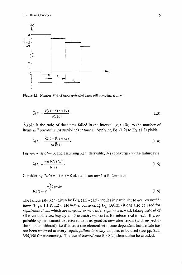
Figure 1.1 Number T(t) of (nonrepairable) items still operating at time t

i ( t ) 6 t is the ratio of the items failed in the interval ( t , t +6t ] to the number of items still operating (or surviving) at time t. Applying Eq. (1.2) to Eq. (1.3) yields

For n+ CQ & St-10, and assuming R( t ) derivable, h(t) converges to the failure rate

-d R(t) l d t h(t> =

R( t )

Considering R(0) = 1 (at t = 0 all items are new) it follows that

The failure rate h ( t ) given by Eqs. (1.3)- (1.5) applies in particular to nonrepairable items (Figs. 1.1 & 1.2). However, considering Eq. (A6.25) it can also be used for repairable items which are as-good-as-new after repair (renewal), taking instead of t the variable X starting by X = 0 ut euch renewal (as for interarrival times). If a repairable system cannot be restored to be as-good-as-new after repair (with respect to the state considered), i.e if at least one element with time dependent failure rate has not been renewed at every repair, failure intensity z ( t ) has to be used (see pp. 355, 356,358 for cornments). The use of hazard rate for A( t ) should also be avoided.


In many practical applications, N t ) = h can be assumed. Eq. (1.6) then yields

for h(t) = h .

The failure-free time T > 0 is exponentially distributed (F( t ) = Pr{% I t } = 1 - e-L ).

For this case, and only in this case, the failure rate h can be estimated by B = k I T , where T is a given (fixed) cumulative operating time and k the total number of failures during T (Eqs. (7.28) and (A8.46)).

The mean (expected value) of the failure-free time T> 0 is given by (Eq. (A6.38))

where MTTF stands for mean time to failure. For k ( t ) = h it follows that E[T] = 11h. Constant (time independent) failure rate h is often assumed for repairable

items too, considered as-good-as-new after repair (renewal). For this case, and only in this case, successive failure-free times are independent random variables, exponentially distributed with the same Parameter A, and have mean

MTBF = l / h , for h(x)= h , (1.9)

where MTBF stands for mean operating time between failures. Also because of the statistical estimate M ~ B F = T l k (Section 7.2.3.1), often used in practical applications, MTBF should be confined to the case of repairable items with constant failure rate (p. 358). For Markov and semi-Markov models, MUTs is used (Eqs. (6.287) or (A7.142)).

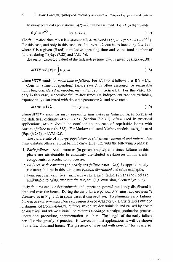
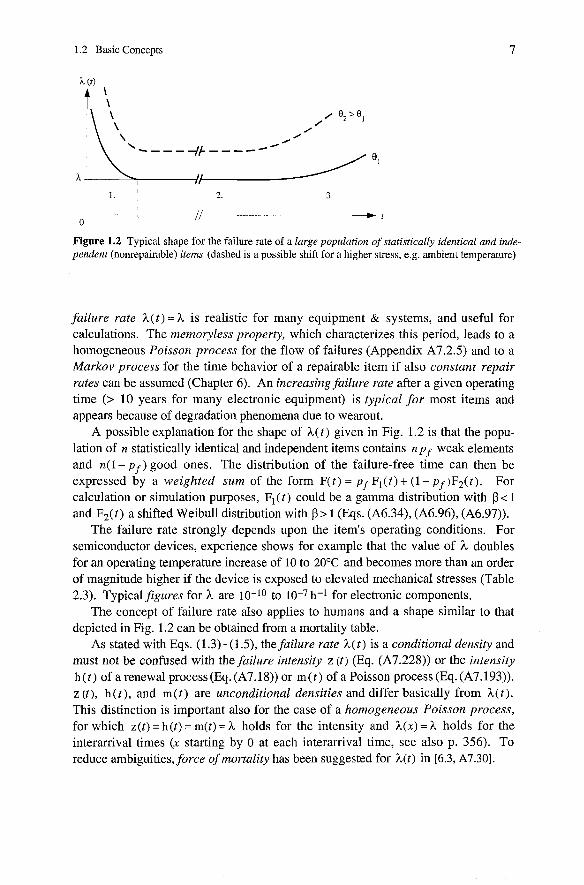
The failure rate of a large population of statistically identical und independent items exhibits often a typical bathtub curve (Fig. 1.2) with the following 3 phases:

1. Early failures: A ( t ) decreases (in general) rapidly with time; failures in this phase are attributable to randomly distributed weaknesses in materials, components, or production processes.

2. Failures with constant (or nearly so) failure rate: h(t) is approximately constant; failures in this period are Poisson distributed and often cataleptic.

3. Wearout failures: h(t) increases with time; failures in this period a r e attributable to aging, wearout, fatigue, etc. (e.g. corrosion, electrornigration).

Early failures are not deterministic and appear in general randomly distributed in time and over the items. During the early failure period, h(t) must not necessarily decrease as in Fig. 1.2, in some cases it can oscillate. To eliminate early failures, bum-in or environmental stress screening is used (Chapter 8). Early failures must be distinguished from systematic failures, which are deterministic and caused by errors or mistakes, and whose elimination requires a change in design, production process, operational procedure, documentation or other. The length of the early failure period varies greatly in practice. However, in most applications it will be shorter than a few thousand hours. The presence of a period with constant (or nearly so)

1.2 Basic Concepts

Figure 1.2 Typical shape for the failure rate of a Zarge population of statistically identical und independent (nonrepairable) items (dashed is a possible shift for a higher Stress, e.g. ambient temperature)

failure rate h ( t ) = h is realistic for many equipment & Systems, and useful for caIcuIations. The memoryless property, which characterizes this period, Ieads to a homogeneous Poisson process for the flow of failures (Appendix A7.2.5) and to a Markov process for the time behavior of a repairable item if also constant repair rates can be assumed (Chapter 6). An increasing failure rate after a given operating time (> 10 years for many electronic equipment) is typical for most items and appears because of degradation phenomena due to wearout.

A possible explanation for the shape of h ( t ) given in Fig. 1.2 is that the population of n statistically identical and independent items contains n pf weak elements and n(1- p f ) good ones. The distribution of the failure-free time can then be expressed by a weighted sum of the form F(t) = pf Fl( t ) + ( 1 - p f ) F z ( t ) . For calculation or simulation purposes, Fl( t ) could be a gamma distribution with ß < 1 and Fz(t ) a shifted Weibull distribution with ß> 1 (Eqs. (A6.34), (A6.96), (A6.97)).

The failure rate strongly depends upon the item's operating conditions. For semiconductor devices, experience shows for example that the value of ?L doubles for an operating temperature increase of 10 to 20°C and becomes more than an order of magnitude higher if the device is exposed to elevated mechanical Stresses (Table 2.3). Typicalfigures for ?L are 10-10 to 10-7 h-1 for electronic components.

The concept of failure rate also applies to humans and a shape similar to that depicted in Fig. 1.2 can be obtained from a mortality table.

As stated with Eqs. (1.3) -(1.5), the failure rate h ( t ) is a conditional density and must not be confused with the failure intensity z ( t ) (Eq. (A7.228)) or the intensity h ( t ) of a renewal process (Eq. (A7.18)) or m ( t ) of a Poisson process (Eq. (A7.193)). z (t) , h ( t ) , and m ( t ) are unconditional densities and differ basically from h ( t ) . This distinction is important also for the case of a homogeneous Poisson process, for which z ( t ) = h( t ) = m(t) = h holds for the intensity and h(x ) = h holds for the interarrival times ( X starting by 0 at each interarrival time, See also p. 356). To reduce ambiguities, force of mortality has been suggested for h(t ) in [6.3, A7.301.

8 1 Basic Concepts, Quality and Reliability Assurance of Complex Equiprnent and Systems

1.2.4 Maintenance, Maintainability

Maintenance defines the set of activities performed on an item to retain it in or to restore it to a specified state. Maintenance is thus subdivided into preventive maintenance, carried out at predetermined intervals to reduce wearout failures, and corrective maintenance, carried out after failure recognition and intended to put the item into a state in which it can again perform the required function. Aim of a preventive maintenance is also to detect and repair hidden failures, i.e. failures in redundant elements not identified at their occurrence. Corrective maintenance is also known as repair, and can include any or all of the following steps: recognition, isolation (localization & diagnosis), elimination (disassembly, replace, reassembly), checkout. Repair is used hereafter as a synonym for restoration. To simplify calculations, it is generally assumed that the element in the reliability block diagram for which a maintenance action has been performed is as-good-as-new after maintenance. This assumption is valid for the whole equipment or system in the case of constant failure rate for all elements which have not been repaired or replaced.

Maintainability is a characteristic of an item, expressed by the probability that a preventive maintenance or a repair of the item will be performed within a stated time intental for given procedures und resources (skill level of personnel, spare Parts, test facilities, etc.). From a qualitative point of view, maintainability can be defined as the ability of an item to be retained in or restored to a specified state. The expected value (mean) of the repair time is denoted by MTTR (mean time to repair), that of a preventive maintenance by MTTPM. Often used for unscheduled removals is also MTBUR. Maintainability has to be built into complex equipment or Systems during design und development by realizing a maintenance concept. Due to the increasing maintenance cost, maintainability aspects have grown in importance. However, maintainability achieved in the field largely depends on the resources available for maintenance (human and material), as well as on the correct installation of the equipment or system, i.e. on the logistic support and accessibility.

1.2.5 Logistic Support

Logistic support designates all activities undertaken to provide effective and economical use of an item during its operating phase. To be effective, logistic support should be integrated into the rnaintenance concept of the item under consideration and include after-sales service.

An emerging aspect related to maintenance and logistic support is that of obsolescence managernent, i.e. how to assure functionality over a long operating period, e.g. 20 years, when technology is rapidly evolving and components need for maintenance are no longer manufactured. Care has to be given here to design aspects, to assure interchangeability during the equipment's useful life without important redesign. Standardization in this direction is in Progress [1.9].


1.2.6 Availability

Availability is a broad term, expressing the ratio of delivered to expected service. It is often designated by A and used for the stationary & steady-state value of the point and average availability (PA = AA). Point availability (PA(t)) is a characteristic of an item expressed by the probability that the item will perform its required function under given conditions at a stated instant of time t. From a qualitative point of view, point availability can be defined as the ability of the item to perjorm its required function under given conditions at a stated instant of time (dependability).

Availability evaluations are often difficult, as logistic support and human factors should be considered in addition to reliability and maintainability. Ideal human and logistic support conditions are thus often assumed, yielding to the intrinsic (inherent) availability. Hereafter, availability is used as a synonym for intrinsic availability. Further assumptions for calculations are continuous operation and complete renewal for the repaired element in the reliability block diagram (assumed as-good-as-new after repair). For a given item, the point availability PA(t) rapidly converges to a stationary & steady-state value, given by (Eq. (6.48))

PA is also the stationary & steady-state value of the average availability (AA) giving the expected value (mean) of the percentage of the time during which the item performs its required function. PAs and AAS is used for considerations at system level. Other availability measures can be defined, e.g. mission availability, work-mission availability, overall availability (Sections 6.2.1.5, 6.8.2). Application specific figures are also known, see e.g. [6.11]. In contrast to reliability analyses for which no failure at item (system) level is allowed (only redundant parts can fail and be repaired on line), availability analyses allow failures at item (system) level.

1.2.7 Safety, Risk, and Risk Acceptance

Safety is the ability of the item not to cause injury to persons, nor significant material damage or other unacceptable consequences during its use. Safety evaluation must consider the following two aspects: Safety when the item functions and is operated correctly and safety when the item or a part of it has failed. The first aspect deals with accident prevention, for which a large number of national and international regulations exist. The second aspect is that of technical safety which is investigated using the same tools as for reliability. However, a distinction between technical safety and reliability is necessary. While safety assurance examines measures which allow an item to be brought into a safe state in the case of failure (fail-safe behavior), reliability assurance deals more generally with measures for minimizing the total number of failures. Moreover, for technical safety the effects of external


influences like human errors, catastrophes, sabotage, etc. are of great importance and must be considered carefully. The safety level of an item influences the number of product liability claims. However, increasing in safety can reduce reliability.

Closely related to the concept of (technical) safety are those of risk, risk management, and risk acceptance, including risk analysis and risk assessment [1.21, 1.261. Risk problems are generally interdisciplinary and have to be solved in close cooperation between engineers und sociologists to find common solutions to controversial questions. An appropriate weighting between probability of occurrence and effect (consequence) of a given accident is important. The multiplicative rule is one among different possibilities. Also it is necessary to consider the different causes (machine, machine & human, human) and effects (location, time, involved people, effect duration) of an accident. Statistical tools can Support risk assessment. However, although the behavior of a homogenous human population is often known, experience shows that the reaction of a single Person can become unpredictable. Similar difficulties also arise in the evaluation of rare events in complex systems. Considerations on risk and risk acceptance should take into account that the probability p, for a given accident which can be caused by one of n statistically identical and independent items, each of them with occurrence probability p, is for np small nearly equal to np as per

Equation (1.11) follows from the binomial distribution and the Poisson approximation (Eqs. (A6.120) & (A6.129)). It also applies with n p = Atot T to the case in which one assumes that the accident occurs randomly in the interval (0, T], caused by one of n independent items (systems) with failure rates Al , ..., L,,, where ?L„, = ?Ll + ... + An . This is because the sum of n independent Poisson processes is again a Poisson process (Eq. (7.27)) and the probability ?L„ ~ e - ~ ~ ~ ~ ~ for one failure in the interval (0, T] is nearly equal to Atot T . Thus, for n p << 1 or Atot T << 1 it holds that

Also by assuming a reduction of the individual occurrence probability p (or failure rate Li), one recognizes that in the future it will be necessary either to accept greater risks p, or to keep the spread of high-risk technologies under tighter control. Similar considerations could also be made for the problem of environmenfal Stresses caused by mankind. Aspects of ecologically acceptable production, use, disposal, and recycling or reuse of products will become subject for international regulations, in the general context of sustainable development.

In the context of a product development, risks related to feasibility and time to market within the given cost constraints must be considered during all development phases (feasibility checks in Fig. 1.6 and Tables A3.3 & 5.3).


Mandatory for risk rnanagement are psychological aspects related to risk awareness and safety communication. As long as a danger for risk is not perceived, people often do not react. Knowing that a safety behavior presupposes a risk awareness, communication is an important tool to avoid that a risk related to the system considered will be underestimated, See e.g. [1.26].

1.2.8 Quality

Quality is understood as the degree to which a set of inherent characteristics fulfiIls requirements. This definition, given now also in the ISO 9000: 2000 IA1.61, follows closely the traditional definition of quality, expressed by fitness for use, and applies to products and services as well.

1.2.9 Cost and System Effectiveness

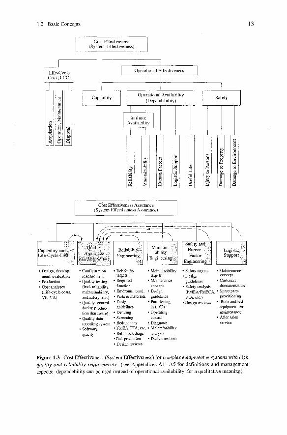
All previously introduced concepts are interrelated. Their relationship is best shown through the concept of cost effectiveness, as given in Fig. 1.3. Cost effectiveness is a measure of the ability of the item to meet a service demand of stated quanti- tative characteristics, with the best possible usefulness to life-cycle cost ratio. It is often referred also to as system effectiveness. Figure 1.3 deals essentially with technical and cost aspects. Some management aspects are considered in Appendices A2 - A 5. From Fig. 1.3, one recognizes the central role of quality assurance, bringing together all assurance activities (Section 1.3.3), and of dependability (collective term for availability performance and its influencing factors).

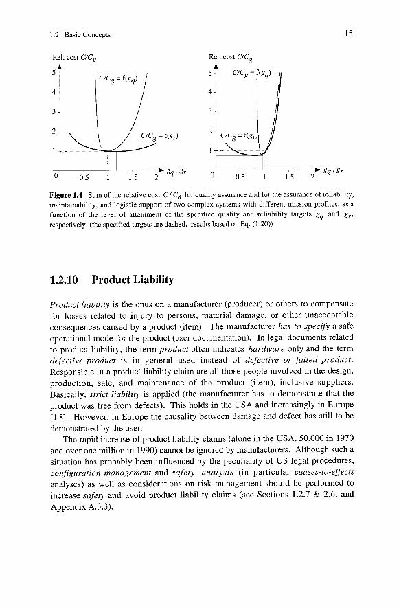
As shown in Fig. 1.3, lije-cycle cost (LCC) is the sum of the cost for acquisition, operation, maintenance, and disposal of an item. For complex systems, higher reliability in general leads to a higher acquisition cost and lower operating cost, so that the optimum of life-cycle cost seldom lies at extremely low or high reliability figures. For such a System, per year operating and maintenance cost often lie between 3 and 6% of acquisition cost, and experience shows that up to 80% of the life-cycle cost is frequently generated by decisions early in the design phase. In the future, life-cycle cost will take more into account current and deferred damage to the environment caused by production, use, and disposal of an item. Life-cycle cost optimization is project specific, in general, and falls within the framework of cost effectiveness or systems engineering. It can be positively influenced by concurrent engineering [1.13, 1.15, 1.221. Figure 1.4 shows as an example the influence of the attainment level of quality and reliability targets on the sum of cost for quality assurance and for the assurance of reliability, maintainability, and logistic support for two complex systems [2.3 (1986)l. To introduce this model, let us first consider Example 1.1.


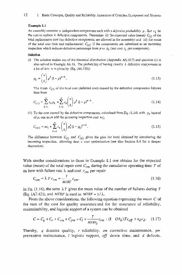
Example 1.1 An assembly contains n independent components each with a defective probability p . Let ck be the cost to replace k defective components. Determine (i) the expected value (mean) C(i) of the total replacement cost (no defective components are allowed in the assembly) and (ii) the mean of the total cost (test and replacement) C(ii) if the components are submitted to an incoming inspection which reduces defective percentage from p to po (test cost ct per component).

Solutiori

(i) The solution makes use of the binomial distribution (Appendix A6.10.7) and question (i) is also solved in Example A6.18. The probability of having exactly k defective components in a lot of size n is given by (Eq. (A6.120))

The mean C(i) of the total cost (deferred cost) caused by the defective components follows then from

(ii) To the cost caused by the defective components, calculated from Eq. (1.14) with p, instead of p, one must add the incoming inspection cost n cl

The difference between C(i) and C(ii) gives the gain (or loss) obtained by introducing the incoming inspection, allowing thus a cost optimization (see also Section 8.4 for a deeper discussion).

With similar considerations to those in Example 1.1 one obtains for the expected value (mean) of the total repair cost C„ during the cumulative operating time T of an item with failure rate h and cost C, per repair

1 C„=hTc„=-

MTBF ccm.

In Eq. (1.16), the term h T gives the mean value of the number of failures during T (Eq. (A7.42)), and MTBF is used as MTBF = 1 / h.

From the above considerations, the following equation expressing the mean C of the sum of the cost for quality assuranceand for the assurance of reliability, maintainability, and logistic support of a system can be obtained

Thereby, q denotes quality, r reliability, crn corrective maintenance, prn preventive maintenance, 1 logistic support, off down time, and d defects.

1.2 Basic Concepts

I Cost Effectiveness (System Effectiveness) I

Capability C11 Ooerational Availability ' 1 . (Dependabili

i Cost Effectiveness Assurance (System Effectiveness Assurance) 1

Safety D

. Design, develop- . Configuration ment, evaiuation management . Production Quality testing Cost analyses (incl. reliability, (Life-cycle costs, maintainability. VE, VA) and safety tests)

Quality control during production (hardware) Quality data reporting System . Software quality

Reliability . Maintainability targets targets . Required . Maintenance function concept . Environm. cond. . Design . Parts & materials guidelines Design . Paititioning guidelines in LRUs . Derating . Operating Screening control . Redundancy . Diagnosis . FMEA, FTA, etc. . Maintainability Rel. block diagr. analysis Rel. prediction . Design reviews Design reviews

. Safety targets . Maintenance . Design concept guidelines . Customer . Safety analysis documentation ( F M E M C A , ' Spare Parts FTA, etc.) provisioning

. ~~~i~~ reviews TOO~S and test equipment for maintenance After d e s service

Figure 1.3 Cost Effectiveness (System Effectiveness) for complex equipment & Systems with high quality und reliability requirements (see Appendices A l - A5 for definitions and management aspects; dependability can be used instead of operational availability, for a qualitative meaning)


MTBFs and OAs are the system mean operating time between failures (assumed here = 1 / hs) and the system steady-state overall availability (Eq. (6.196) with Tpm

instead of T„). T is the total system operating time (useful life) and nd is the number of hidden defects discovered (and eliminated) in the field. Cq , C r , Ccm , C„, and Cl are the cost for quality assurance and for the assurance of reliability, repairability, serviceability, and logistic support, respectively. C„, c o f ~ , and cd are the cost per repair, per down time hour, and per hidden defect, respectively (preventive maintenance cost are scheduled cost, considered here as a part of Cpm).

The first five terms in Eq. (1.17) represent a part of the acquisition cost, the last three terms are deferred cost occurring during field operation. A model for investigating the cost C according to Eq. (1.17) was developed in [2.3 (1986)l by assuming C q , C,., Ccm, Cpm, C I , MTBFS, OAS, T, cm, C,#, and cd as Parameters and investigating the variation of the total cost expressed by Eq. (1.17) as a function of the level of attainment of the specified targets, i.e. by introducing the variables gq = QA IQA, , gr = MTBFs I MTBFs,, g„ = MTIRSg~MTTRs, gpm = MTTPMS, / MTTPMS, and gl = MLDsg I MLDs, where the subscript g denotes the specified target for the corresponding quantity. A power relationship

was assumed between the actual cost C i , the cost Ci, to reach the specified target (goal) of the considered quantity, and the level of attainment of the specified target ( 0 i ml < 1 and all other mi > I). The following relationship between the number of hidden defects discovered in the field and the ratio C9 / C , was also included in the model

The final equation for the cost C as function of the variables g9, gr , g, , g„ , and gl follows then as (using Eq. (6.196) for OAs)

The relative cost C / C , given in Fig. 1.4 is obtained by dividing C by the value C , form Eq. (1.20) with all gi = 1. Extensive analyses with different values for mi, C i , MTBFs, OAs, T, C,, cs8, and cd have shown that the value C / Cg is only moderately sensitive to the parameters mi.

1.2 Basic Concepts

Rel. cost C/Cg

Figure 1.4 Sum of the relative cost C / Cg for quality assurance and for the assurance of reliability, maintainability, and logistic support of two complex Systems with different mission profiles, as a function of the level of attainment of the specified quality and reliability targets gq and g„ respectively (the specified targets are dashed, results based on Eq. (1.20))

1.2.10 Product Liability

Product liability is the onus on a manufacturer (producer) or others to compensate for losses related to injury to persons, material damage, or other unacceptable consequences caused by a product (item). The manufacturer has to speczfy a safe operational mode for the product (user documentation). In legal documents related to product liability, the term product often indicates hardware only and the term defective product is in general used instead of defective or failed product. Responsible in a product liability claim are all those people involved in the design, production, sale, and maintenance of the product (item), inclusive suppliers. Basically, strict liability is applied (the manufacturer has to demonstrate that the product was free from defects). This holds in the USA and increasingly in Europe [1.8]. However, in Europe the causality between damage and defect has still to be demonstrated by the wer.

The rapid increase of product liability claims (alone in the USA, 50,000 in 1970 and over one million in 1990) cannot be ignored by manufacturers. Although such a situation has probably been influenced by the peculiarity of US legal procedures, configuration management and safety analysis (in particular causes-to-effects analyses) as well as considerations on risk management should be performed to increase safety and avoid product liability claims (see Sections 1.2.7 & 2.6, and Appendix A.3.3).


1.2.11 Historical Development

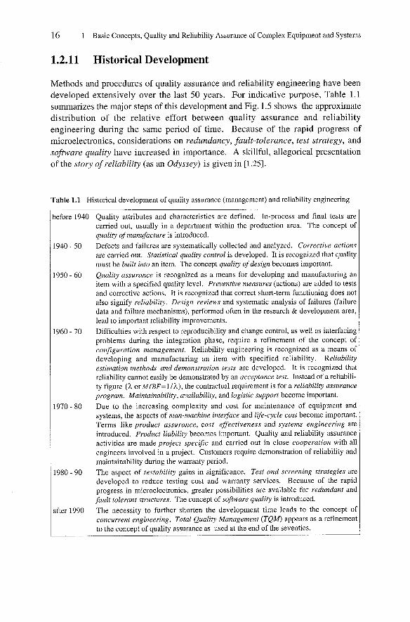
Methods and procedures of quality assurance and reliability engineering have been developed extensively over the last 50 years. For indicative purpose, Table 1.1 summarizes the major steps of this development and Fig. 1.5 shows the approximate distribution of the relative effort between quality assurance and reliability engineering during the same period of time. Because of the rapid progress of microelectronics, considerations on redundancy, fault-tolerante, test strategy, and sojhvare quality have increased in importance. A skillful, allegorical presentation of the story of reliability (as an Odyssey) is given in [1.25].

Table 1.1 Histoncal development of quality assurance (management) and reliability engineering

~efore 1940 Quality attributes and characteristics are defined. In-process and final tests are

L940 - 50

1950 - 60

1960 - 70

1970 - 80

1980 - 90

after 1990

carried out, usually in a department within the production area. The concept of quality of manufacture is introduced.

Defects and failures are systematically collected and analyzed. Corrective actions are carried out. Statistical quality control is developed. It is recognized that quality must be built into an item. The concept quality of design becomes important.

Quality assurance is recognized as a means for developing and manufacturing an item with a specified quality level. Preventive measures (actions) are added to tests and corrective actions. It is recognized that correct short-term functioning does not also signify reliability. Design reviews and systematic analysis of failures (failure data and failure mechanisms), performed often in the research & development area, lead to important reliability improvements.

Difficulties with respect to reproducibility and change control, as well as interfacing problems during the integration phase, require a refinement of the concept of configuration management. Reliability engineering is recognized as a means of developing and manufacturing an item with specified reliability. Reliability estimation methods und demonstration tests are developed. It is recognized that reliability cannot easily be demonstrated by an acceptance test. Instead of a reliability figure (h orMTBF=lIh), the contractual requirement is for a reliability assurance program. Maintainability, availability, and logistic Support become important.

Due to the increasing complexity and cost for maintenance of equipment and systems, the aspects of man-machine interface and life-cycle cost become important. Terms like product assurance, cost effectiveness and systems engineering are introduced. Product liability becomes important. Quality and reliability assurance activities are made project specific and carried out in close cooperation with all engineers involved in a project. Customers require demonstration of reliability and maintainability during the warranty penod. The aspect of testability gains in significance. Test und screening strategies are developed to reduce testing cost and warranty services. Because of the rapid progress in microelectronics, greater possibilities are available for redundant and fault tolerant structures. The concept of sofhvare quality is introduced. The necessity to further shorten the development time leads to the concept of concurrent engineering. Total Quality Management (TQM) appears as a refinement to the concept of quality assurance as used at the end of the seventies.

Alessandro Birolini Reliability Engineering · Prof. Dr. Alessandro Birolini ∗ Ponte Vecchio –...

Documents

Transcript of Alessandro Birolini Reliability Engineering · Prof. Dr. Alessandro Birolini ∗ Ponte Vecchio –...