Alessandra Bianchini and Carlos R. Gonzalez April 2012 ... · Alessandra Bianchini and Carlos R....
40
ERDC/GSL TR-12-15 Pavement-Transportation Computer Assisted Structural Engineering (PCASE) Implementation of the Modified Berggren (ModBerg) Equation for Computing the Frost Penetration Depth within Pavement Structures Geotechnical and Structures Laboratory Alessandra Bianchini and Carlos R. Gonzalez April 2012 Approved for public release; distribution is unlimited.
Transcript of Alessandra Bianchini and Carlos R. Gonzalez April 2012 ... · Alessandra Bianchini and Carlos R....
ERD
C/G
SL T
R-1
2-1
5
Pavement-Transportation Computer Assisted Structural Engineering (PCASE) Implementation of the Modified Berggren (ModBerg) Equation for Computing the Frost Penetration Depth within Pavement Structures
Geo
tech
nic
al a
nd
Str
uct
ure
s La
bor
ator
y
Alessandra Bianchini and Carlos R. Gonzalez April 2012
Approved for public release; distribution is unlimited.
ERDC/GSL TR-12-15 April 2012
Pavement-Transportation Computer Assisted Structural Engineering (PCASE) Implementation of the Modified Berggren (ModBerg) Equation for Computing the Frost Penetration Depth within Pavement Structures Alessandra Bianchini and Carlos R. Gonzalez
Geotechnical and Structures Laboratory U.S. Army Engineer Research and Development Center 3909 Halls Ferry Road Vicksburg, MS 39180-6199
Final report
Approved for public release; distribution is unlimited.
Prepared for U.S. Army Corps of Engineers Washington, DC 20314-1000
ERDC/GSL TR-12-15 ii
Abstract
The design of pavement structures in cold climates must account for the changes in soil properties due to the influence of freezing and thawing cycles. The calculation of the frost penetration depth is a fundamental step in the design and evaluation of pavement structures by the U.S. Department of Defense (DoD). To compute the frost penetration, the DoD currently uses the modified Berggren (ModBerg) equation. The Unified Facilities Criteria (UFC) 3-130-06 includes a methodology to manually compute the frost depth. The Pavement-Transportation Computer Assisted Structural Engineering (PCASE) software incorporates a more accurate numerical solution of the ModBerg equation, which in some instances provides slightly different values than the manual solution described in the UFC. Researchers from the U.S. Army Engineer Research and Development Center (ERDC) realized the need to explain why the same procedure results in different values of the frost depth, and sought to reaffirm the importance of advanced numerical tools in pavement design and evaluation. The objective of this report is to present the solution of the heat equation applied to a one-dimensional homogeneous and isotropic layer, which is currently implemented in the PCASE software. The report also explains the differences between the UFC- and PCASE-computed solutions.
DISCLAIMER: The contents of this report are not to be used for advertising, publication, or promotional purposes. Citation of trade names does not constitute an official endorsement or approval of the use of such commercial products. All product names and trademarks cited are the property of their respective owners. The findings of this report are not to be construed as an official Department of the Army position unless so designated by other authorized documents. DESTROY THIS REPORT WHEN NO LONGER NEEDED. DO NOT RETURN IT TO THE ORIGINATOR.
ERDC/GSL TR-12-15 iii
Contents Abstract ................................................................................................................................................... ii
Figures and Tables ................................................................................................................................. iv
Preface ..................................................................................................................................................... v
Unit Conversion Factors ........................................................................................................................ vi
1 Introduction ..................................................................................................................................... 1
Background .............................................................................................................................. 2 Objective ................................................................................................................................... 4 Report content .......................................................................................................................... 4
2 Definitions of Basic Concepts and Variables .............................................................................. 5
Heat flux .................................................................................................................................... 5 Freezing or thawing season ..................................................................................................... 5 Air- and surface-freezing, or thawing, index ............................................................................ 5 The n-factor ............................................................................................................................... 6 Thermal conductivity ................................................................................................................ 6 Specific heat ............................................................................................................................. 7 Volumetric heat capacity .......................................................................................................... 7 Volumetric latent heat of fusion .............................................................................................. 8 Thermal resistance .................................................................................................................. 8 Thermal diffusivity .................................................................................................................... 9 Thermal ratio ............................................................................................................................ 9 Fusion parameter ................................................................................................................... 10 The coefficient λ ..................................................................................................................... 10
3 The Fourier’s Law and the Modified Berggren (ModBerg) Equation ...................................... 11
The Fourier’s law .................................................................................................................... 11 The heat equation .................................................................................................................. 12 The Stefan’s equation ............................................................................................................ 14 The modified Berggren (ModBerg) equation ........................................................................ 14
4 Computation of Frost Depth Penetration for Layer Systems .................................................. 21
PCASE procedure for computing frost depth ........................................................................ 21 Computation example ............................................................................................................ 22
Computer solution ...................................................................................................................... 23
Manual solution.......................................................................................................................... 24 Comparison of the PCASE and manual solutions ................................................................. 29
5 Conclusions ................................................................................................................................... 31
References ............................................................................................................................................ 32
Report Documentation Page
ERDC/GSL TR-12-15 iv
Figures and Tables
Figures
Figure 1. Thawing or freezing front within the soil layer system. ......................................................... 17
Figure 2. Average thermal conductivity for sands and gravels, frozen (UFC 3-130-06). ................... 25
Figure 3. Average thermal conductivity for silt and clay soils, frozen (UFC 3-130-06). ..................... 25
Figure 4. Average volumetric heat capacity for soils (UFC 3-130-06). ................................................ 26
Figure 5. Average latent heat for soils (UFC 3-130-06). ....................................................................... 27
Figure 6. λ coefficient in the ModBerg equation (UFC 3-130-06). ...................................................... 28
Tables
Table 1. Relative accuracy of different solutions (Nixon and McRoberts 1973). ................................. 4
Table 2. Pavement characteristics. ......................................................................................................... 22
Table 3. Multilayer solution of the ModBerg equation. ......................................................................... 26
ERDC/GSL TR-12-15 v
Preface
The design of pavement structures in cold climates must account for the changes in soil properties due to the influence of freezing and thawing cycles. The calculation of frost depth is a fundamental step during the design and evaluation of pavement structures by the U.S. Department of Defense (DoD). The DoD uses the modified Berggren (ModBerg) equation to compute the frost penetration depth.
The Unified Facilities Criteria (UFC) 3-130-06 includes a methodology to manually compute the frost depth. The Pavement-Transportation Computer Assisted Structural Engineering (PCASE) software incorporates a more comprehensive numerical solution of the ModBerg equation, which in some instances predicts values slightly different than the manual solution described in the UFC. Researchers with the Engineer Research and Development Center (ERDC) realized the need to explain why the same procedure results in different values of the frost depth, and sought to reaffirm the importance of advanced numerical tools in pavement design and evaluation. This report explains the fundamental theory behind the calculation of the frost depth, and documents how PCASE and the UFC implement the ModBerg solution.
Personnel of ERDC’s Geotechnical and Structures Laboratory (GSL), Vicksburg, Mississippi, prepared this publication. The researchers were Carlos R. Gonzalez and Dr. Alessandra Bianchini, Airfields and Pavements Branch (APB), GSL. The analysis of the frost depth calculations and PCASE implementation was conducted by Gonzalez. Bianchini prepared this report under the supervision of Dr. Gary L. Anderton, Chief, APB; Dr. Larry N. Lynch, Chief, Engineering Systems and Materials Division (ESMD); Dr. William P. Grogan, Deputy Director, GSL; and Dr. David W. Pittman, Director, GSL.
At the time of publication, COL Kevin J. Wilson was Commander and Executive Director of ERDC. Dr. Jeffery P. Holland was Director.
ERDC/GSL TR-12-15 vi
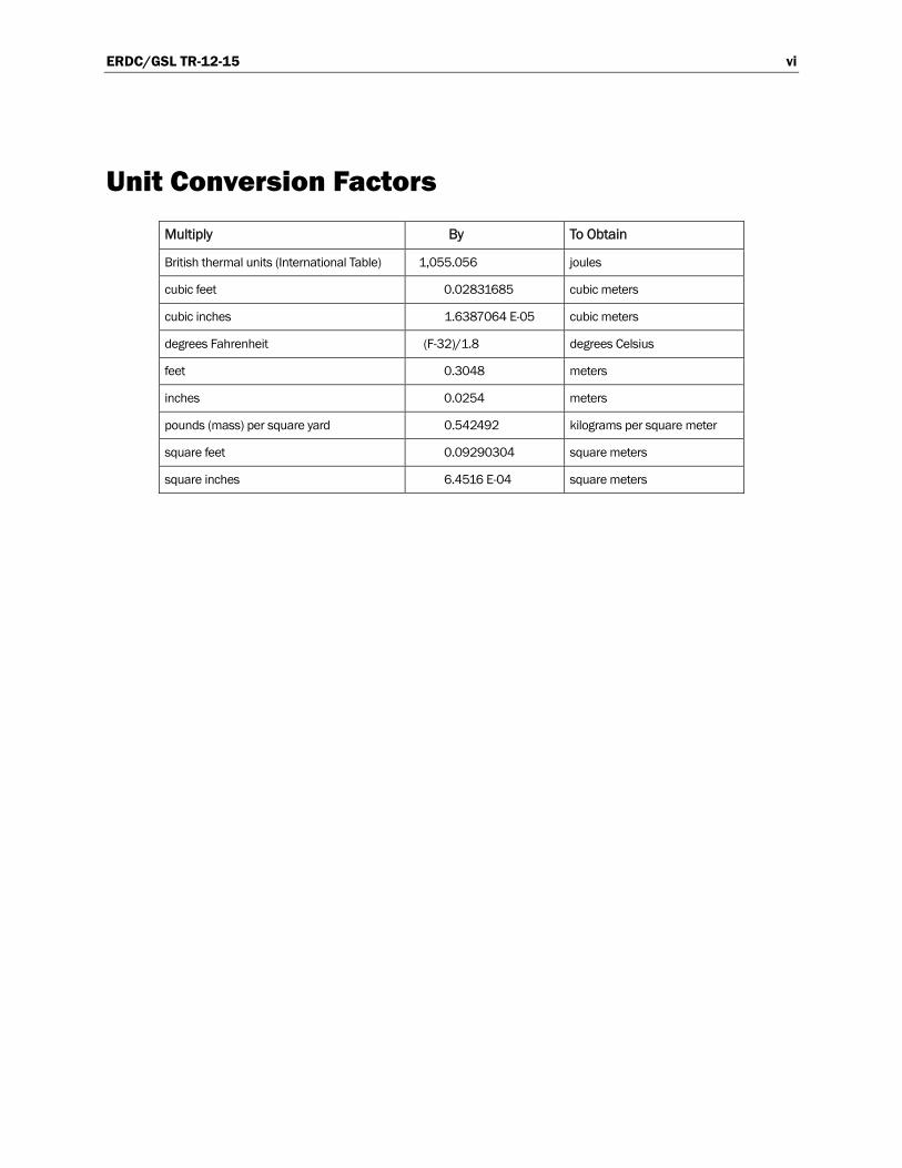
Unit Conversion Factors
Multiply By To Obtain
British thermal units (International Table) 1,055.056 joules
cubic feet 0.02831685 cubic meters
cubic inches 1.6387064 E-05 cubic meters
degrees Fahrenheit (F-32)/1.8 degrees Celsius
feet 0.3048 meters
inches 0.0254 meters
pounds (mass) per square yard 0.542492 kilograms per square meter
square feet 0.09290304 square meters
square inches 6.4516 E-04 square meters
ERDC/GSL TR-12-15 1
1 Introduction
The design of pavement structures in areas susceptible to freezing and thawing cycles must consider the influence of such cycles on structural performance. The mechanical properties of the soil layers and the material hydraulic conductivity change upon freezing. Frost heave damages the pavement structure by increasing the volume of the underlying frost-susceptible soils. During thawing, the structural characteristics of the frost-susceptible soils drastically diminish, therefore limiting the pavement capabilities in supporting the design traffic. Evaluation of the frost penetra-tion depth is a fundamental step during the design and evaluation of pavement structures.
The frost depth formula initially was provided by Stefan in 1889 and later revised. Stefan’s formula tended to overestimate the frost depth in temperate zones because it neglected the volumetric heat (Paynter 1999). The modified Berggren (ModBerg) equation represents the current formula to adequately estimate the frost depth and overcomes the limitations of Stefan’s formula. The ModBerg equation is the solution of the one-dimensional heat transfer differential equation through a homogeneous and isotropic medium.
The Unified Facilities Criteria (UFC) 3-130-06, Calculation Methods for Determination of Depth of Freeze and Thaw in Soil: Arctic and Subarctic Construction, includes the methodology to manually compute the frost depth, using average values of soil and climate parameters. With the development of high-speed computers, it now is possible to numerically solve the heat transfer differential equation through a layered media and provide a more comprehensive solution.
The Pavement-Transportation Computer Assisted Structural Engineering (PCASE) software incorporates the numerical solution of the heat transfer equation, therefore providing slightly different values than the manual solution, as instructed in the UFC 3-130-06. An Engineer Research and Development Center (ERDC) research team realized the need to explain why the PCASE and the UFC procedures give different values of frost penetration depth, and sought to reaffirm the importance of advanced numerical tools in pavement design and evaluation.
ERDC/GSL TR-12-15 2
The objective of this report is to present the solution of the heat equation applied to a one-dimensional homogeneous and isotropic layer, which is currently implemented in the PCASE software. The report also explains the significances of the differences between the PCASE and UFC solutions.
Background
In cold climates, engineers must consider the effects of soil freezing and thawing cycles when designing any structure, in particular pavement structures. Pavements, either rigid or flexible, consist of a layered structure that includes granular materials, with each layer capable of sustaining portions of the applied static and dynamic loads. The soil moisture content, temperature distribution within the soil mass, depth of frost penetration, migration of the water within the soil upon freezing, and rate of thawing all influence the pavement’s structural capability.
In frost-susceptible soils, the major problem induced by freezing is the creation of frost heave and the continuous migration of moisture toward the freezing zone. The knowledge of the frost penetration depth gives pavement engineers the ability to take remedial measures and mitigate the influence of frost on the performance of pavement systems. One measure consists of removing and replacing any frost-susceptible soil with non-susceptible soils, thus avoiding heaving.
A major problem arises during the thawing season, when the frozen moisture starts the changing phase. Upon thawing, the soils are saturated, and the drop in effective stresses determines a decrease in the soil shear strength that is proportional to the effective normal stress. Thus, pavements have greatly reduced structural capabilities during thawing. The structural capability is gradually regained as the excess moisture drains, restoring normal soil moisture content and density.
Studies of ground freezing and thawing cycles and soil properties started in the 1950s, with a U.S. Army Corps of Engineers-sponsored research program, and are ongoing. The objective was to compute the frost penetra-tion depth occurring in temperate climates and the annual thaw in perma-frost zones. Several models and laboratory experiments were evaluated, and resulted in the adoption of the ModBerg equation currently in common use (Paynter 1999).
ERDC/GSL TR-12-15 3
One of the difficulties in developing theoretical models representing real-case scenarios was how to account for the effect of the latent heat during ground freezing or thawing. As Brown (1964) pointed out, the latent heat release, or absorption, over a range of temperatures introduces non-linearity to the problem associated with heat transfer. An additional complicating factor is that soils are not homogeneous with respect to their constituents and, in particular, with respect to moisture content, which might vary greatly within the layer, especially in that portion close to the surface. Furthermore, soil properties vary depending on whether the soil is in a frozen or unfrozen state (Brown 1964; Nixon and McRoberts 1973).
One of the approaches for computing the frost penetration depth employs the Neumann solution (Lunardini 1980). It takes into consideration the soil latent heat and its influence on the frost depth, which varies inversely with the square root of the soil latent heat. This solution assumes a homogeneous soil initially at a constant temperature above or below freezing that under-goes a sudden change at the surface to a constant temperature below or above freezing. Brown (1964) highlighted some of the inaccuracies of the Neumann solution, one being the assumption of the constant moisture content within the soil mass. The moisture content varies with depth and time, and such changes induce variations of the soil thermal properties. Moreover, in many soils, moisture does not freeze at exactly 32°F, rather within a range of temperatures. Thus, the latent heat also becomes a variable quantity.
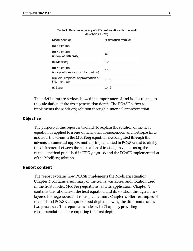
Nixon and McRoberts (1973) compared the frost penetration depth values computed through different theoretical or empirical models. The models included the Neumann rigorous analytical solution for a step surface temperature change; the modified Neumann solution independent of the ratio of frozen and unfrozen soil diffusivity; the ModBerg equation by Aldrich and Paynter (1953); the modified Neumann solution for which the temperature distribution was ignored; the semi-empirical approximation of the modified Neumann solution independent of temperature distribution; and the Stefan equation with a linear temperature profile in the thawed zone. Taking the Neumann analytical solution as reference, Table 1 shows the relative accuracy of the solution computed with each model. The comparison showed that accuracy increases with the rise in computational efforts, and empirical models tend to overestimate the frost depth.
ERDC/GSL TR-12-15 4
Table 1. Relative accuracy of different solutions (Nixon and McRoberts 1973).
Model solution % deviation from (a)
(a) Neumann --
(b) Neumann (indep. of diffusivity)
0.0
(c) ModBerg 1.8
(d) Neumann (indep. of temperature distribution)
11.0
(e) Semi-empirical approximation of Neumann (a) 11.0
(f) Stefan 14.2
The brief literature review showed the importance of and issues related to the calculation of the frost penetration depth. The PCASE software implements the ModBerg solution through numerical approximation.
Objective
The purpose of this report is twofold: to explain the solution of the heat equation as applied to a one-dimensional homogeneous and isotropic layer and how the terms in the ModBerg equation are computed through the advanced numerical approximations implemented in PCASE; and to clarify the differences between the calculation of frost depth values using the manual method published in UFC 3-130-06 and the PCASE implementation of the ModBerg solution.
Report content
The report explains how PCASE implements the ModBerg equation. Chapter 2 contains a summary of the terms, variables, and notation used in the frost model, ModBerg equations, and its application. Chapter 3 contains the rationale of the heat equation and its solution through a one-layered homogeneous and isotropic medium. Chapter 4 offers examples of manual and PCASE computed frost depth, showing the differences of the two processes. The report concludes with Chapter 5 providing recommendations for computing the frost depth.
ERDC/GSL TR-12-15 5
2 Definitions of Basic Concepts and Variables
This section contains definitions of specific terms, basic concepts, and variables used in heat transfer calculations applied to soils or pavement structures. Some of the definitions are in the UFC 3-130-06 and in the Technical Manual (TM) 5-852-1/Air Force Manual (AFM) 88-19 Chapter 1, Arctic and Subarctic Construction General Provisions.
Heat flux
The heat flux is the amount of heat, or energy, transferred in a medium per unit of time through a unit area. The direction of the flow is temperature dependent and ranges from regions at higher temperature to regions at lower temperatures. In general, heat transfer occurs through conduction, convection, or radiation.
The freezing or thawing of soils is the result of the temperature differentials between two regions and the induced heat flux. The time rate of change in the heat transfer depends on the temperature differential and the soil thermal properties. The penetration of the freezing or thawing temperature into the soil mass depends also on the duration of the temperature differential at the ground-air interface and on the thermal regime of the soil. The thermal regime is the temperature pattern existing in a soil body in relation to the seasonal variations.
Freezing or thawing season
The freezing or thawing season is that period of time, measured in days, during which the average daily temperature is below or above 32°F.
Air- and surface-freezing, or thawing, index
The freezing or thawing index is the number of degree-days between the highest and lowest points on a curve of cumulative degree-days versus time for one freezing or thawing season. The index quantifies the magnitude and duration of below- or above-freezing temperatures occurring during any given freezing or thawing season.
ERDC/GSL TR-12-15 6
The air-freezing or air-thawing index refers to the temperature measured approximately 4.5 ft above the ground. The surface-freezing or surface-thawing index is computed based upon the temperature measured below the surface.
The n-factor
There is no simple correlation between air-freezing or air-thawing and surface-freezing or surface-thawing indices. Nevertheless, for practical purposes, the n-factor is the parameter employed to represent the correlation between air-freezing or air-thawing and surface-freezing or surface-thawing indices. The n-factor is the ratio of surface index to air index for either freezing or thawing.
Representative values of the n-factor are available in published literature. However, an accurate determination of such a factor for a specific location requires concurrent measurements of air and surface temperatures during several complete freezing and thawing seasons, along with predicted future changes in seasonal temperature values.
Thermal conductivity
The thermal conductivity K is the quantity of heat flow in a unit time through a unit area of a material caused by a unit thermal gradient. K is expressed in British thermal unit (Btu) per foot (Btu/ft hr °F).
In soils, the thermal conductivity depends on several factors such as soil density, moisture content, particle shape, temperature, air-filled voids, and the state of the pore water (if frozen or unfrozen). The UFC 3-130-06 contains several charts for determining the value of K for different types of soils and in relation to the silt and clay content of the soil.
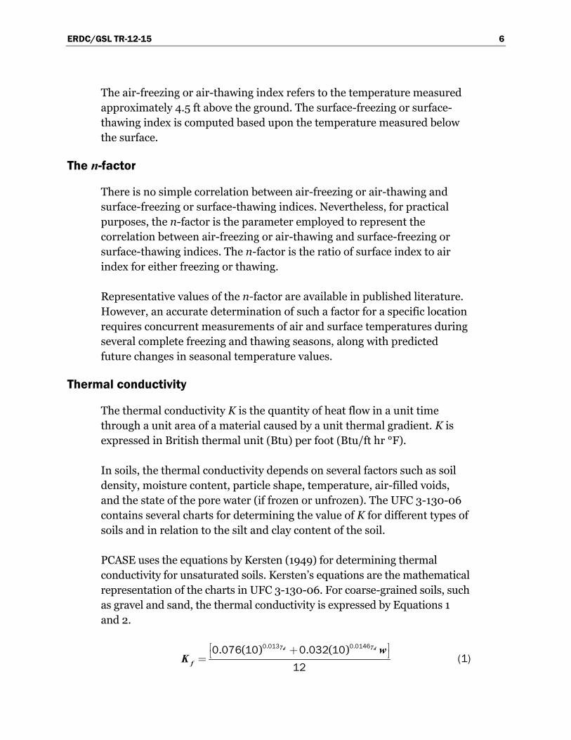
PCASE uses the equations by Kersten (1949) for determining thermal conductivity for unsaturated soils. Kersten’s equations are the mathematical representation of the charts in UFC 3-130-06. For coarse-grained soils, such as gravel and sand, the thermal conductivity is expressed by Equations 1 and 2.
. .. ( ) . ( )é ù+ë û=
0 013 0 01460 076 10 0 032 10
12
d dγ γ
f
wK (1)
ERDC/GSL TR-12-15 7
( ) .( . log . )é ù+ë û=
0 010 7 0 4 10
12
dγ
u
wK (2)
where
γd = soil dry unit weight w = soil water content in percentage
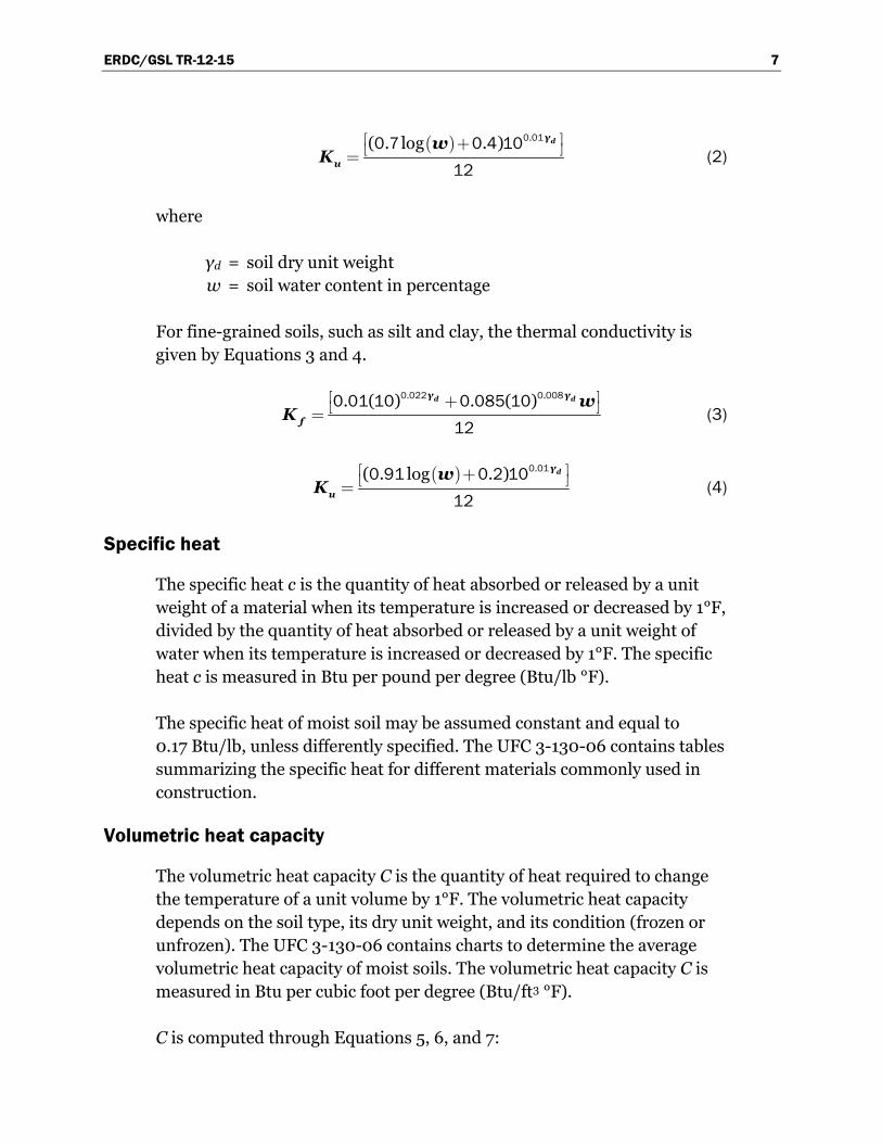
For fine-grained soils, such as silt and clay, the thermal conductivity is given by Equations 3 and 4.
. .. ( ) . ( )é ù+ë û=
0 022 0 0080 01 10 0 085 10
12
d dγ γ
f
wK (3)
( ) .( . log . )é ù+ë û=
0 010 91 0 2 10
12
dγ
u
wK (4)
Specific heat
The specific heat c is the quantity of heat absorbed or released by a unit weight of a material when its temperature is increased or decreased by 1°F, divided by the quantity of heat absorbed or released by a unit weight of water when its temperature is increased or decreased by 1°F. The specific heat c is measured in Btu per pound per degree (Btu/lb °F).
The specific heat of moist soil may be assumed constant and equal to 0.17 Btu/lb, unless differently specified. The UFC 3-130-06 contains tables summarizing the specific heat for different materials commonly used in construction.
Volumetric heat capacity
The volumetric heat capacity C is the quantity of heat required to change the temperature of a unit volume by 1°F. The volumetric heat capacity depends on the soil type, its dry unit weight, and its condition (frozen or unfrozen). The UFC 3-130-06 contains charts to determine the average volumetric heat capacity of moist soils. The volumetric heat capacity C is measured in Btu per cubic foot per degree (Btu/ft3 °F).
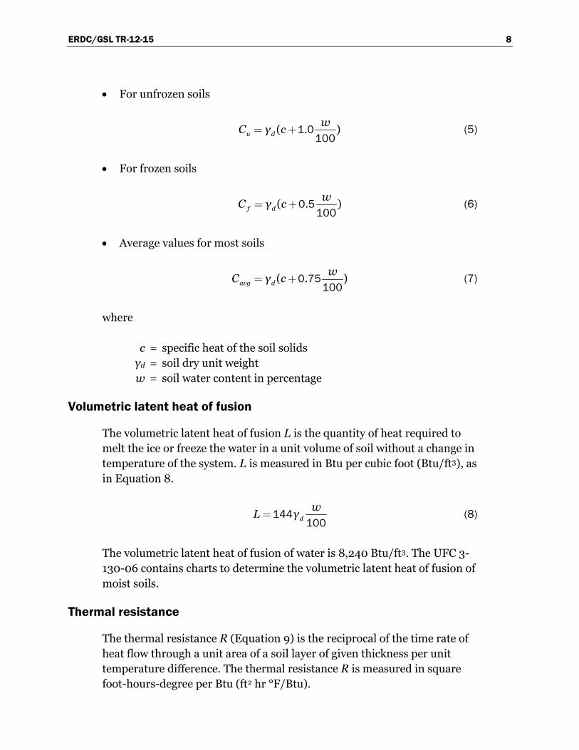
C is computed through Equations 5, 6, and 7:
ERDC/GSL TR-12-15 8
For unfrozen soils
u d
wC γ c( . )= +1 0
100 (5)
For frozen soils
f d
wC γ c( . )= +0 5
100 (6)
Average values for most soils
avg d
wC γ c( . )= +0 75
100 (7)
where
c = specific heat of the soil solids γd = soil dry unit weight w = soil water content in percentage
Volumetric latent heat of fusion
The volumetric latent heat of fusion L is the quantity of heat required to melt the ice or freeze the water in a unit volume of soil without a change in temperature of the system. L is measured in Btu per cubic foot (Btu/ft3), as in Equation 8.
d
wL γ=144
100 (8)
The volumetric latent heat of fusion of water is 8,240 Btu/ft3. The UFC 3-130-06 contains charts to determine the volumetric latent heat of fusion of moist soils.
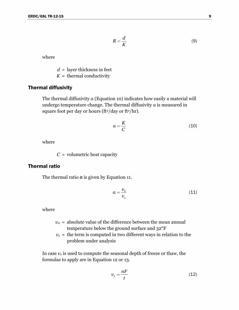
Thermal resistance
The thermal resistance R (Equation 9) is the reciprocal of the time rate of heat flow through a unit area of a soil layer of given thickness per unit temperature difference. The thermal resistance R is measured in square foot-hours-degree per Btu (ft2 hr °F/Btu).
ERDC/GSL TR-12-15 9
d
RK
= (9)
where
d = layer thickness in feet K = thermal conductivity
Thermal diffusivity
The thermal diffusivity a (Equation 10) indicates how easily a material will undergo temperature change. The thermal diffusivity a is measured in square foot per day or hours (ft2/day or ft2/hr).
K
aC
= (10)
where
C = volumetric heat capacity
Thermal ratio
The thermal ratio α is given by Equation 11.
s
v
vα = 0 (11)
where
v0 = absolute value of the difference between the mean annual temperature below the ground surface and 32°F
vs = the term is computed in two different ways in relation to the problem under analysis
In case vs is used to compute the seasonal depth of freeze or thaw, the formulas to apply are in Equation 12 or 13.
s
nFv
t= (12)
ERDC/GSL TR-12-15 10
or
s
nIv
t= (13)
where
n = conversion factor from air index to surface index F = air-freezing index I = air-thawing index t = length of the freezing or thawing season
If vs is used to compute the multiyear freeze of thaw depths that might develop as a result of some long-term change in the heat balance at the ground surface, the formulas above do not apply. In this case, vs is the absolute value of the difference between the mean annual ground surface temperature and 32°F.
Fusion parameter
The fusion parameter µ is a function of vs, and therefore has a different value in relation to the problem under analysis. The fusion parameter is in Equation 14.
s
Cμ v
L= (14)
The coefficient λ
The coefficient λ is a factor allowing for heat capacity and initial temperature of the ground. The coefficient λ is a function of the fusion parameter µ and thermal ratio α, and generally indicated as λ = f(µ,α)
ERDC/GSL TR-12-15 11
3 The Fourier’s Law and the Modified Berggren (ModBerg) Equation
This section contains definitions of the Fourier’s Law of heat conduction, heat equation, and its mathematical derivation. The one-dimensional case of the heat equation, its application to a layered system, and the computation of the frost depth also are explained.
The Fourier’s law
The Fourier’s law represents the basis of the models used to compute the depth of frost penetration. The law states that the rate of heat transfer, with respect to time through a material, is proportional to the negative gradient of the temperature function and to the surface area of the material mass.
The mathematical general formula of the Fourier’s law is in Equation 15.
q kA u=- (15)
where
q = heat flux k = positive constant A = surface area of the material mass through which there is heat
exchange = gradient of the temperature function
For the one-dimensional case, the Fourier’s law reduces to Equation 16.
q kAu
x
¶=-
¶ (16)
The Fourier’s law also is applied to derive the heat equation in its differential form. The following paragraph shows the derivation of the heat equation.
ERDC/GSL TR-12-15 12
The heat equation
The heat equation is a parabolic partial differential equation that represents the process of heat propagation through a continuous medium. In general terms, the heat equation has the following form (Equation 17):
tu k uΔ- =0 (17)
where
ut = first derivative of the function u(x, t) with respect to t k = positive constant Δ = the Laplacian operator
In the study of the heat flow in a three-dimensional space, Equation 15 can be obtained with the following derivation.
Let D be a region in R3, x = [x1, x2, x3] a vector in R3, u(x, t) the temperature at point x and time t. The total amount of heat H(t) contained in the region D is given by Equation 18.
( ) ( )D
H t cρu x t dx,= ò (18)
where
c = specific heat of the material ρ = material density
The change in heat with time is expressed in Equation 19.
( )t
D
dHcρu x t dx
dt,= ò (19)
The change in heat occurs if there are regions at different temperatures. In fact, the Fourier’s law states that the heat flows from regions at higher temperatures to regions with lower temperature values at a rate κ>0, proportional to the temperature gradient. In addition, since the heat flow is possible exclusively through the region boundary ∂D, it results in Equation 20.
ERDC/GSL TR-12-15 13
D
dHκ u ndS
dt
= ⋅ò (20)
where
n = outward unit vector normal to the surface S κ = constant = the gradient operator
Applying the divergence theorem to Equation 20 gives Equation 21.
( )D D
κ u ndS κ dxu
⋅ = ⋅ ò ò (21)
Combining Equation 19 and 21 results in Equation 22.
( ) ( )t
D D
cρu x t dx κ dx, u= ⋅ ò ò (22)
Removing the operation of integration and solving the scalar product on the right-hand side of Equation 22 results in Equation 23.
tcρu κ uΔ= (23)
With κ
kcρ
= >0, Equation 23 can be rewritten as Equation 24, which
equals Equation 17.
tu k uΔ= (24)
The one-dimensional heat equation is simply a restriction of the general form of Equation 24. For unforced heat, the heat equation is Equation 25.
u
kt
ux
¶ ¶=
¶ 
2
2 (25)
ERDC/GSL TR-12-15 14
The Stefan’s equation
The Stefan’s equation was one of the first formulations for computing frost depths. The equation was developed by Josef Stefan in 1889, within a study about ice formation and melting in the Polar Oceans. The predicting formula for frost depth is Equation 26.
Stefan
knFX
L=
48 (26)
where
XStefan = frost depth as per Stefan k = thermal conductivity of the material n = correlation factor F = air-freezing index L = latent heat
The formula does not consider the volumetric heat, and therefore tends to overestimate the frost depth. Numerous studies were developed to provide more accurate predictions of frost depth, producing values closer to those measured in the field (Paynter 1999). The ModBerg equation, explained in the following sections, is the model currently adopted by the DoD for frost depth computation.
The modified Berggren (ModBerg) equation
Starting from the Fourier’s law (Equation 27) and to quantify the heat transferred through a homogeneous isotropic material, such as a soil layer, it is possible to derive the ModBerg equation. The ModBerg equation provides the depth within the soil that is reached by the frost line.
u
q kAx
¶=-
¶ (27)
where
q = heat flow rate A = surface area k = thermal conductivity of the material
ERDC/GSL TR-12-15 15
The minus sign in Equation 27 indicates the direction of the heat flux that is opposite to the direction of the temperature increase. Integrating Equation 27 for a soil layer of thickness X, where the temperature at the upper and lower surfaces are T1 and T2 (T1<T2), respectively, results in Equations 28 to 30.
qdx kAdu=- (28)
TX
T
qdx kAdu=-ò ò2
10
(29)
( )qX kA T T= -1 2 (30)
Therefore, the rate of heat flow is expressed in Equation 31.
( )kA T T
qX
-= 1 2 (31)
Multiplying q by the time interval dt, the total amount of heat Qc transferred during the interval dt is given by Equation 32.
( )
c
kA T T dtQ qdt
X
-= = 1 2 (32)
A specific quantity of heat must be removed from the soil mass to induce freezing. The volumetric latent heat of fusion L indicates the amount of heat required to freeze the water in a unit volume of soil without a change in temperature of the system. For an element of soil dV = Adx, the total heat needed to freeze the water within its voids is in Equation 33.
VQ LdV LAdx= = (33)
For thermal equilibrium, equating the expressions 28 and 29 gives Equation 34.
( )kA T T dt
LAdxX
-=1 2 (34)
Rearranging and simplifying Equation 34 results in Equation 35.
ERDC/GSL TR-12-15 16
( )k T T dt
XdxL
-=1 2 (35)
The integration of Equation 35 (re-ordered) is Equation 36.
( )t
X kT T dt
L= -ò
2
1 2
02
(36)
Considering that the temperature differential T1-T2 is constant between the two surfaces, and that freezing is assumed to occur at 32°F, the integral term of the right-hand side of Equation 36 is the surface-freezing index I, and Equation 36 can be rewritten as Equation 37.
X k
IL
=2
2 (37)
The ModBerg model’s assumption is that the temperature differential T1-T2 is constant and is equal to the average of the differences between the annual mean temperature and the freezing temperature (32°F).
In Equation 37, X represents the depth at which the material will reach the freezing temperature. The depth X of frost penetration is equal to Equation 38.
kI
XL
=2
(38)
Equation 38 is formally similar to the Stefan’s equation, aside from a multiplying factor of 24 that was used in the Stefan’s equation for unit consistency. The use of the Stefan’s equation produced overestimated values of the frost depth compared to those measured in the field. For this reason, several studies were conducted to introduce a correction factor and, therefore, provide values of the frost depth more in agreement with measured values. The ModBerg equation is one of those models that predicts frost depth values closer to those measured in the field.
The main contribution of the ModBerg equation is the correction factor λ applied to Equation 38 to produce more realistic values of the frost depth. The correction factor λ was developed from an analysis of the so-called
ERDC/GSL TR-12-15 17
“melting problem” and how the temperature and the latent heat vary within a frozen soil mass system.
When a frozen mass of soil, assumed homogeneous, is subjected at its surface to a temperature above its melting point, the system tends to restore temperature balance within the soil mass through heat conduction. There-fore, thawing temperature will start moving into the frozen soil mass. Assuming that the latent heat is released during the water phase change from solid to liquid at 32°F, the surface temperature does not change. In this case, the solution to the “melting problem” is less complex and can be handled mathematically through approximation. Carslaw and Jaeger (1959) provided a generalized version of the solution initially computed by Neumann (1860), including the soil mass latent heat and sensible heat. The report by Lunardini (1980) showed the solution application to soil systems. The “freezing problem” can be similarly analyzed as the freezing front, instead of the thawing front, will move into the soil mass.
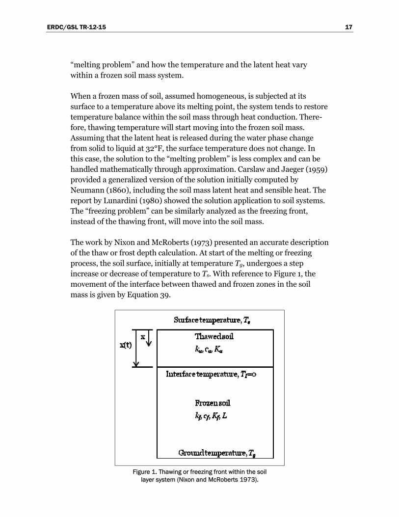
The work by Nixon and McRoberts (1973) presented an accurate description of the thaw or frost depth calculation. At start of the melting or freezing process, the soil surface, initially at temperature Tg, undergoes a step increase or decrease of temperature to Ts. With reference to Figure 1, the movement of the interface between thawed and frozen zones in the soil mass is given by Equation 39.
Figure 1. Thawing or freezing front within the soil
layer system (Nixon and McRoberts 1973).
ERDC/GSL TR-12-15 18
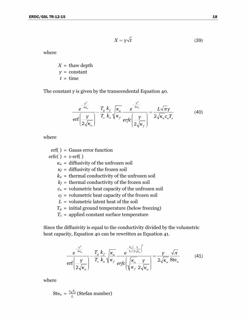
X γ t= (39)
where
X = thaw depth γ = constant t = time
The constant γ is given by the transcendental Equation 40.
fu
γγκκ
g f u
s u f u u s
u f
T k κe e L πγ
T k κ κ c Tγ γerfc
κ κerf
--
- =æ ö æ ö÷ ÷ç ç÷ ÷ç ç÷ ÷ç ç÷ ÷ç ÷è ø çè ø
22
44
2
2 2
(40)
where
erf( ) = Gauss error function erfc( ) = 1-erf( ) κu = diffusivity of the unfrozen soil κf = diffusivity of the frozen soil ku = thermal conductivity of the unfrozen soil kf = thermal conductivity of the frozen soil cu = volumetric heat capacity of the unfrozen soil cf = volumetric heat capacity of the frozen soil L = volumetric latent heat of the soil Tg = initial ground temperature (below freezing) Ts = applied constant surface temperature
Since the diffusivity is equal to the conductivity divided by the volumetric heat capacity, Equation 40 can be rewritten as Equation 41.
u
f uu
κ γγκ κκ
g f u
s u f uu
fu u
T k κe e γ πT k κ κγ κ γ
erfcκκ κ
uSteerf
æ ö÷ç ÷ç-- ÷ç ÷÷çè ø
- =æ ö æ ö÷ ÷ç ç÷ ÷ç ç÷ ÷ç ç÷ ÷ç çè ø è ø
22
24
2
2 2
(41)
where
Steu = (Stefan number)
ERDC/GSL TR-12-15 19
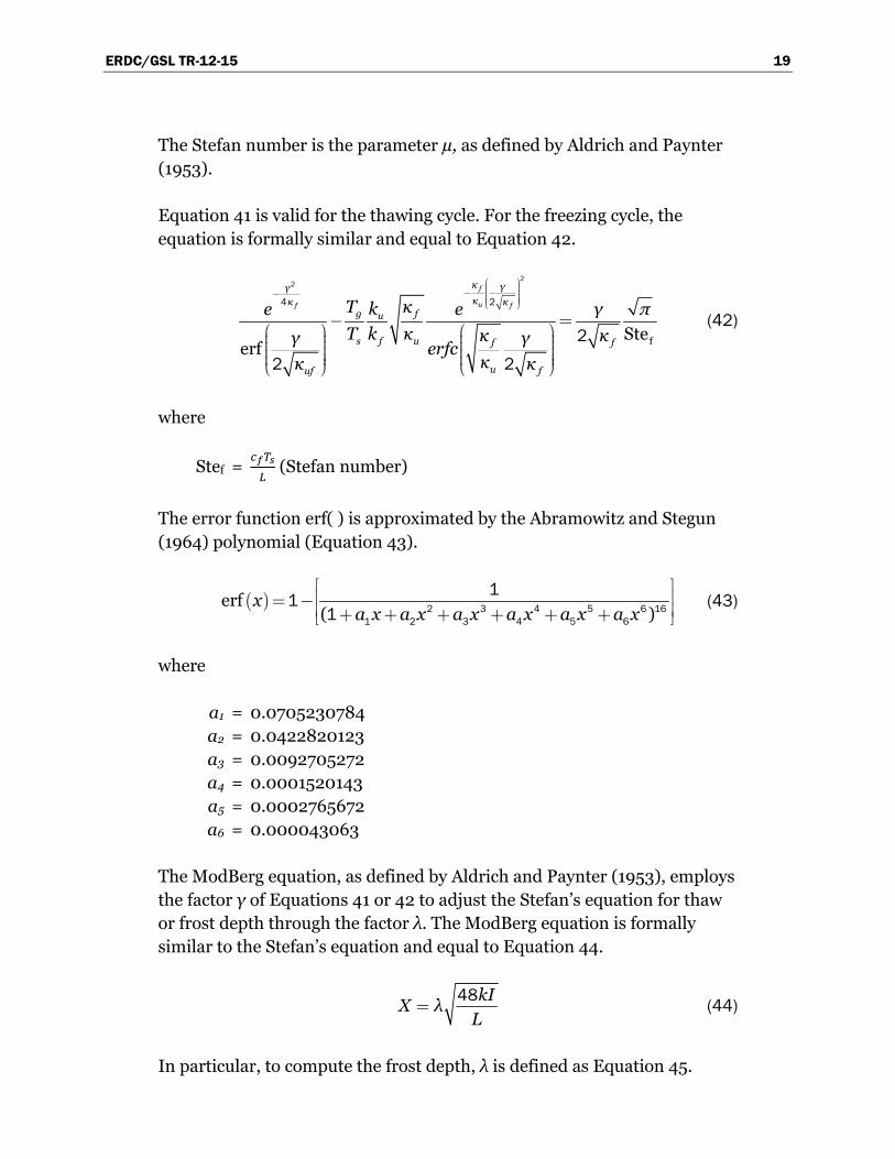
The Stefan number is the parameter µ, as defined by Aldrich and Paynter (1953).
Equation 41 is valid for the thawing cycle. For the freezing cycle, the equation is formally similar and equal to Equation 42.
f
uf f
κ γγκκ κ
g fu
s f u f f
uuf f
T κke e γ πT k κ κ κγ γ
erfcκκ κ
fSteerf
æ ö÷ç ÷ç- ÷- ç ÷ç ÷÷çè ø
- =æ ö æ ö÷ ÷ç ç÷ ÷ç ç÷ ÷ç ç÷ ÷÷ ÷ç çè ø è ø
22
4 2
2
2 2
(42)
where
Stef = (Stefan number)
The error function erf( ) is approximated by the Abramowitz and Stegun (1964) polynomial (Equation 43).
( )xa x a x a x a x a x a x
erf( )
é ùê ú= -ê ú+ + + + + +ë û
2 3 4 5 6 161 2 3 4 5 6
11
1 (43)
where
a1 = 0.0705230784 a2 = 0.0422820123 a3 = 0.0092705272 a4 = 0.0001520143 a5 = 0.0002765672 a6 = 0.000043063
The ModBerg equation, as defined by Aldrich and Paynter (1953), employs the factor γ of Equations 41 or 42 to adjust the Stefan’s equation for thaw or frost depth through the factor λ. The ModBerg equation is formally similar to the Stefan’s equation and equal to Equation 44.
kI
X λL
=48
(44)
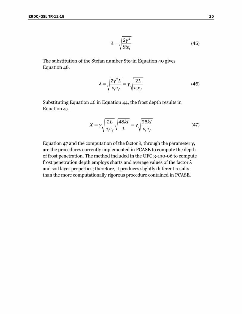
In particular, to compute the frost depth, λ is defined as Equation 45.
ERDC/GSL TR-12-15 20
γ
λStef
=22
(45)
The substitution of the Stefan number Stef in Equation 40 gives Equation 46.
s f s f
γ L Lλ γ
v c v c= =
22 2 (46)
Substituting Equation 46 in Equation 44, the frost depth results in Equation 47.
s f s f
L kI kIX γ γ
v c L v c= =
2 48 96 (47)
Equation 47 and the computation of the factor λ, through the parameter γ, are the procedures currently implemented in PCASE to compute the depth of frost penetration. The method included in the UFC 3-130-06 to compute frost penetration depth employs charts and average values of the factor λ and soil layer properties; therefore, it produces slightly different results than the more computationally rigorous procedure contained in PCASE.
ERDC/GSL TR-12-15 21
4 Computation of Frost Depth Penetration for Layer Systems
This chapter describes the characteristics of the PCASE computer procedure and its iteration in the computation of the frost penetration depth.
The ModBerg method, developed by Aldrich and Paynter (1953), used average values of soil, frozen or unfrozen; specific heats; and thermal diffusivities to allow manual solution of the frost depth problem. The PCASE computer routine uses actual values and, therefore, provides more accurate results than the manual solution.
This chapter presents the computation of the frost penetration depth based on the procedure published in the UFC 3-130-06 and as it is currently implemented in PCASE. The input data are the same for the two cases, but the degree of accuracy and approximation of the two methods differ.
PCASE procedure for computing frost depth
The software routine implemented in PCASE originally was developed by Zarling et al. (1989). The Alaska Department of Transportation subse-quently adopted the same procedure (Braley and Connor 1989).
The required inputs of the user are moisture content and dry density of the soil in each layer. The asphalt or Portland cement concrete (PCC) layer has a default-set moisture content of 0%. The software uses these physical properties to compute the frozen and unfrozen soil thermal properties.
The other input parameters needed for the frost depth calculation are associated with the geographical location where the pavement structure is to be constructed and are included in the climatic database as part of the PCASE Depth of Frost Penetration Calculator. The database includes parameters such as air-freezing index, mean annual temperature, length of frost season, and n-factor for numerous nationwide and worldwide loca-tions. Local weather stations provided these records, which are periodically updated.
ERDC/GSL TR-12-15 22
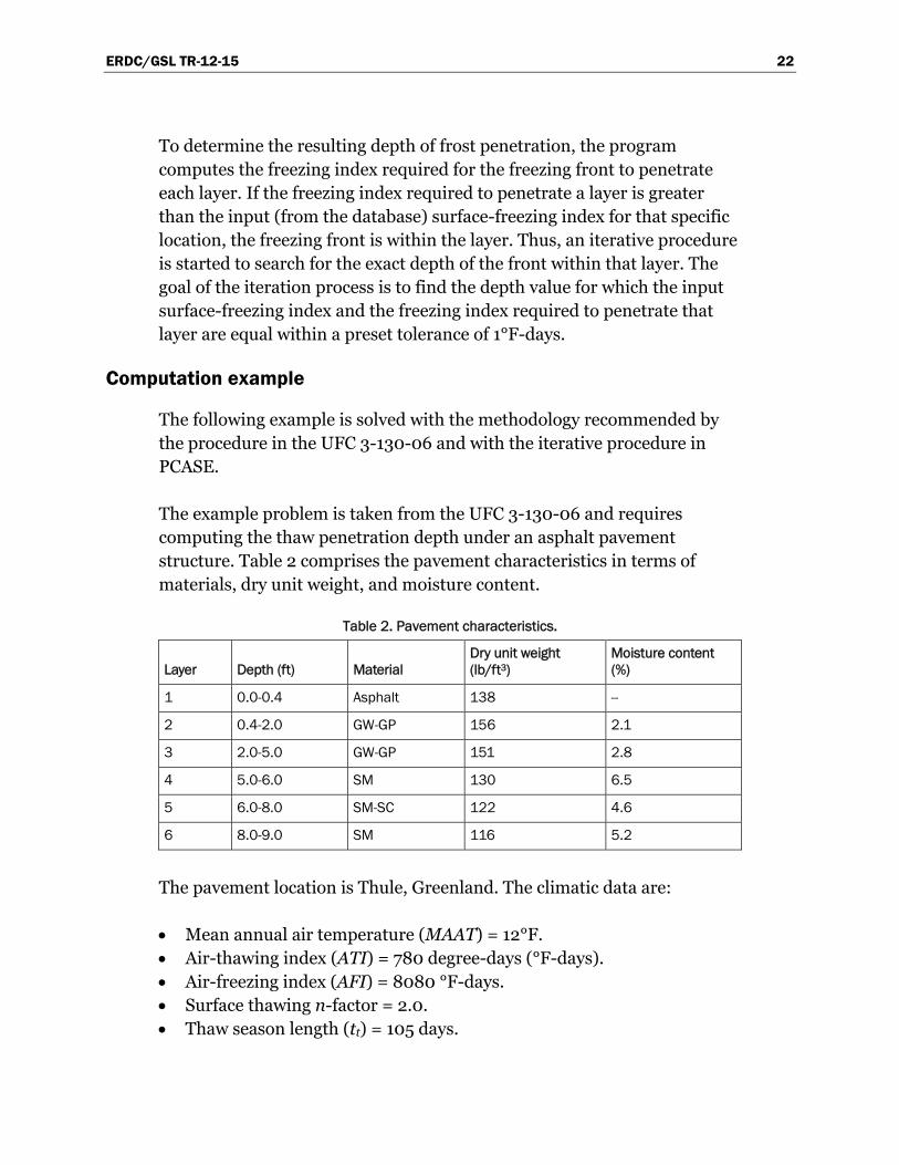
To determine the resulting depth of frost penetration, the program computes the freezing index required for the freezing front to penetrate each layer. If the freezing index required to penetrate a layer is greater than the input (from the database) surface-freezing index for that specific location, the freezing front is within the layer. Thus, an iterative procedure is started to search for the exact depth of the front within that layer. The goal of the iteration process is to find the depth value for which the input surface-freezing index and the freezing index required to penetrate that layer are equal within a preset tolerance of 1°F-days.
Computation example
The following example is solved with the methodology recommended by the procedure in the UFC 3-130-06 and with the iterative procedure in PCASE.
The example problem is taken from the UFC 3-130-06 and requires computing the thaw penetration depth under an asphalt pavement structure. Table 2 comprises the pavement characteristics in terms of materials, dry unit weight, and moisture content.
Table 2. Pavement characteristics.
Layer Depth (ft) Material Dry unit weight (lb/ft3)
Moisture content (%)
1 0.0-0.4 Asphalt 138 --
2 0.4-2.0 GW-GP 156 2.1
3 2.0-5.0 GW-GP 151 2.8
4 5.0-6.0 SM 130 6.5
5 6.0-8.0 SM-SC 122 4.6
6 8.0-9.0 SM 116 5.2
The pavement location is Thule, Greenland. The climatic data are:
Mean annual air temperature (MAAT) = 12°F. Air-thawing index (ATI) = 780 degree-days (°F-days). Air-freezing index (AFI) = 8080 °F-days. Surface thawing n-factor = 2.0. Thaw season length (tt) = 105 days.
ERDC/GSL TR-12-15 23
The surface-thawing index is given by the formula nI and equal to 1,560 °F-days.
Computer solution
The routine in PCASE computes the thaw or frost penetration depth in a layered system by evaluating the portion of the ATI or AFI required to move the thawing or freezing isotherm front through each layer. The sum of these partial depths represents the total depth of thaw or freeze. Each step employs the actual soil characteristics of the thermal diffusivities and heat capacities for computing the layer’s thermal resistance and the coefficient λ rather than average values. For the i-th layer, Equation 48 determines the partial ATIi (or AFIi) index in °F-days is
i
i i ii n
ni
L d RATI R
λ N
-
=
æ ö÷ç= + ÷ç ÷÷çè øå1
2124 2
(48)
where
Li = latent heat (Btu/ft3) di = layer thickness (ft) λi = coefficient Ri = thermal resistance (hr °F/Btu) n = factor
The thermal resistance Ri is equal to Equation 49.
ii
i
dR
K= (49)
where
Ki = thermal conductivity (Btu/hr ft °F)
The software computes the partial index ATIi (or AFIi) for each layer. If the sum is greater than the surface index input of the problem, the thawing front is then located within the i-th layer. The software’s next step is to adjust the apparent thickness of the i-th layer to get convergence to the surface-thawing index input value. Iteration ends when the sum of partial indices is within ±1°F of the target input index.
ERDC/GSL TR-12-15 24
To compute the coefficient λi, the software iterates on each layer. For the i-th layer, λi is defined as Equation 50.
i
s i
Lλ
Cγ
v=
2 (50)
where
vs = average surface temperature differential γ = parameter = equivalent volumetric heat capacity (Btu/ft3 °F) = equivalent latent heat of fusion (Btu/ft3)
The parameter γ is computed by solving Equation 41 through iteration. The average surface temperature differential vs is equal to Equation 51.
st
n ATIv
t
= (51)
The equivalent volumetric heat capacity is equal to Equation 52.
n
i iii n
ii
C d
dC =
=
=åå
1
1
(52)
The equivalent latent heat of fusion is equal to Equation 53.
n
i iii n
ii
L d
dL =
=
=åå
1
1
(53)
With the pavement data in Table 2 and the climatic characteristics of Thule, the computer solution for the thawing depth is equal to 6.78 ft.
Manual solution
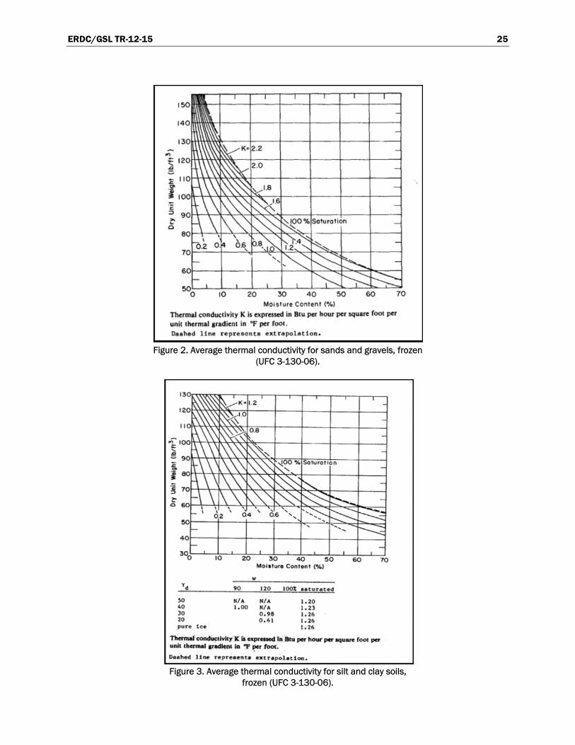
The manual solution employs charts and nomographs in the UFC 3-130-06. The thermal properties of each layer, C, K, and L, are obtained from Figures 2 through 6. Table 3 summarizes layer characteristics values and the manual solution of the problem.
ERDC/GSL TR-12-15 25
Figure 2. Average thermal conductivity for sands and gravels, frozen
(UFC 3-130-06).
Figure 3. Average thermal conductivity for silt and clay soils,
frozen (UFC 3-130-06).
ERDC/GSL TR-12-15 26
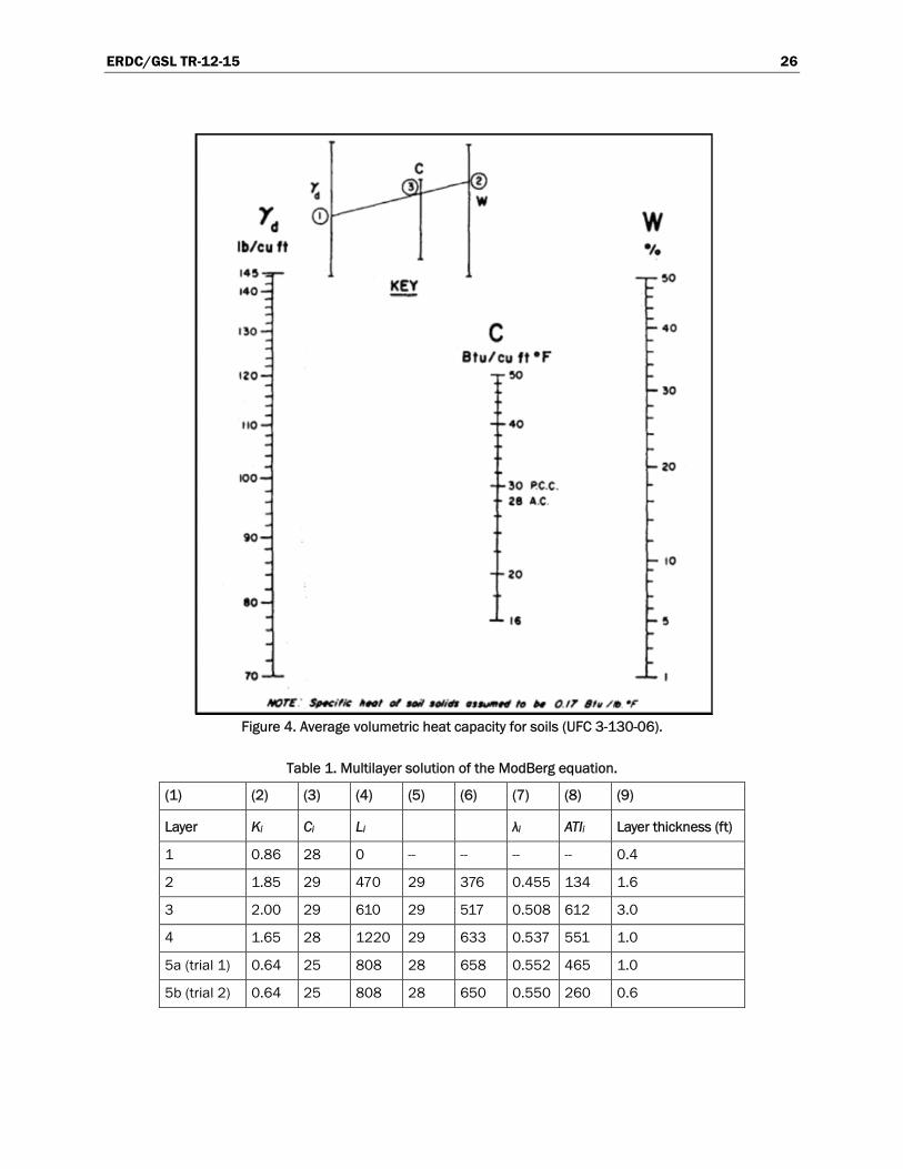
Figure 4. Average volumetric heat capacity for soils (UFC 3-130-06).
Table 1. Multilayer solution of the ModBerg equation.
(1) (2) (3) (4) (5) (6) (7) (8) (9)
Layer Ki Ci Li λi ATIi Layer thickness (ft)
1 0.86 28 0 -- -- -- -- 0.4
2 1.85 29 470 29 376 0.455 134 1.6
3 2.00 29 610 29 517 0.508 612 3.0
4 1.65 28 1220 29 633 0.537 551 1.0
5a (trial 1) 0.64 25 808 28 658 0.552 465 1.0
5b (trial 2) 0.64 25 808 28 650 0.550 260 0.6
ERDC/GSL TR-12-15 27
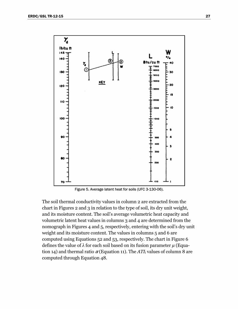
Figure 5. Average latent heat for soils (UFC 3-130-06).
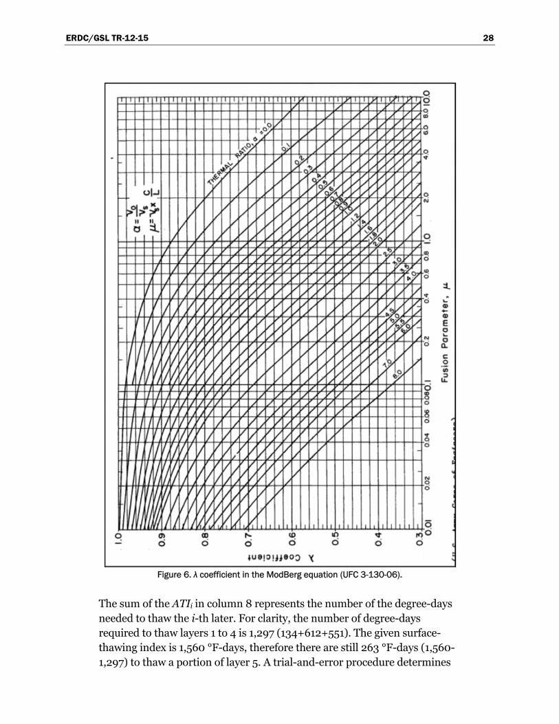
The soil thermal conductivity values in column 2 are extracted from the chart in Figures 2 and 3 in relation to the type of soil, its dry unit weight, and its moisture content. The soil’s average volumetric heat capacity and volumetric latent heat values in columns 3 and 4 are determined from the nomograph in Figures 4 and 5, respectively, entering with the soil’s dry unit weight and its moisture content. The values in columns 5 and 6 are computed using Equations 52 and 53, respectively. The chart in Figure 6 defines the value of λ for each soil based on its fusion parameter µ (Equa-tion 14) and thermal ratio α (Equation 11). The ATIi values of column 8 are computed through Equation 48.
ERDC/GSL TR-12-15 28
Figure 6. λ coefficient in the ModBerg equation (UFC 3-130-06).
The sum of the ATIi in column 8 represents the number of the degree-days needed to thaw the i-th later. For clarity, the number of degree-days required to thaw layers 1 to 4 is 1,297 (134+612+551). The given surface-thawing index is 1,560 °F-days, therefore there are still 263 °F-days (1,560-1,297) to thaw a portion of layer 5. A trial-and-error procedure determines
ERDC/GSL TR-12-15 29
the thickness of layer 5 that will undergo thawing. The first trial is done by setting the thickness of layer 5 equal to 1.0 ft. To thaw 1.0 ft of layer 5 requires 465 °F-days, which is more than the available (263 °F-days). Through proportion, another trial (trial 2) with a thickness of 0.6 ft results in 260 °F-days for thawing it. This result can be considered acceptable in relation to the accuracy provided by the charts and nomographs. To conclude, the thaw penetration depth is equal to 6.6 ft (0.4+1.6+3.0+1.0+0.6).
Comparison of the PCASE and manual solutions
The method implemented in PCASE and the one included in the UFC 3-130-06, Calculation Methods for Determination of Depth of Freeze and Thaw in Soil: Arctic and Subarctic Construction, are essentially the same. The only difference is how the values of the parameters characterizing the soils and the degree of approximation are determined. With regard to the parameters, the method in PCASE uses actual, rather than average, values for the thermal diffusivity, heat capacity, and the factor λ. The latter is determined with Equation 50, where the parameter γ derives from the iteration of Equation 40, as shown below.
i
s i
Lλ
Cγ
v=
2 (bis 50)
fu
γγκκ
g f u
s u f u u s
u f
T k κe e L πγ
T k κ κ c Tγ γerfc
κ κerf
--
- =æ ö æ ö÷ ÷ç ç÷ ÷ç ç÷ ÷ç ç÷ ÷ç ÷è ø çè ø
22
44
2
2 2
(bis 40)
In the UFC, the factor λ is determined from the chart in Figure 6, entering with the average parameters computed through Equations 14 and 11 below.
s
Cμ v
L= (bis 14)
s
v
vα = 0 (bis 11)
In addition, PCASE computes the soil thermal conductivity K through Equations 1 and 2 for coarse-grained soils, and Equations 3 and 4 for fine-
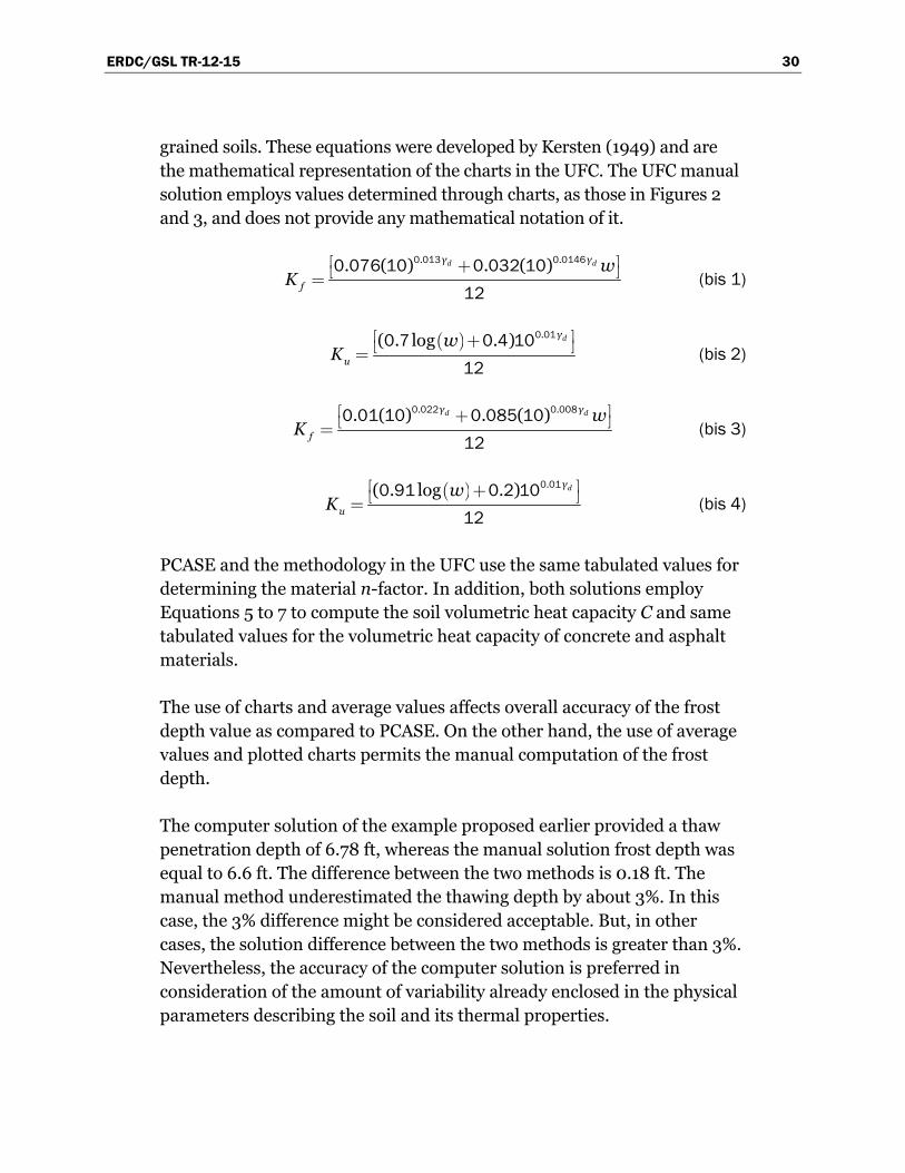
ERDC/GSL TR-12-15 30
grained soils. These equations were developed by Kersten (1949) and are the mathematical representation of the charts in the UFC. The UFC manual solution employs values determined through charts, as those in Figures 2 and 3, and does not provide any mathematical notation of it.
d dγ γ
f
wK
. .. ( ) . ( )é ù+ë û=0 013 0 01460 076 10 0 032 10
12 (bis 1)
( ) dγ
u
wK
.( . log . )é ù+ë û=0 010 7 0 4 10
12 (bis 2)
d dγ γ
f
wK
. .. ( ) . ( )é ù+ë û=0 022 0 0080 01 10 0 085 10
12 (bis 3)
( ) dγ
u
wK
.( . log . )é ù+ë û=0 010 91 0 2 10
12 (bis 4)
PCASE and the methodology in the UFC use the same tabulated values for determining the material n-factor. In addition, both solutions employ Equations 5 to 7 to compute the soil volumetric heat capacity C and same tabulated values for the volumetric heat capacity of concrete and asphalt materials.
The use of charts and average values affects overall accuracy of the frost depth value as compared to PCASE. On the other hand, the use of average values and plotted charts permits the manual computation of the frost depth.
The computer solution of the example proposed earlier provided a thaw penetration depth of 6.78 ft, whereas the manual solution frost depth was equal to 6.6 ft. The difference between the two methods is 0.18 ft. The manual method underestimated the thawing depth by about 3%. In this case, the 3% difference might be considered acceptable. But, in other cases, the solution difference between the two methods is greater than 3%. Nevertheless, the accuracy of the computer solution is preferred in consideration of the amount of variability already enclosed in the physical parameters describing the soil and its thermal properties.
ERDC/GSL TR-12-15 31
5 Conclusions
The design of pavement structures in cold climates must account for the influence of freezing and thawing cycles. The structure performance can be considerably affected by the variability of the soil strength and its structural support. In fact, soil mechanical properties change upon freezing and thawing. The evaluation of frost penetration depth represents an important component in the design and evaluation of pavement structures.
The ModBerg equation is the basis for the procedure currently used by DoD agencies to estimate frost or thaw penetration front. Questions were raised with regard to the differences between the solutions procedure in the UFC 3-130-06, Calculation Methods for Determination of Depth of Freeze and Thaw in Soil: Arctic and Subarctic Construction, and the method implemented in PCASE. The analysis in this report aimed to clarify the differences between the UFC and PCASE solutions. The following conclusions were made:
1. The frost penetration depth formula initially was provided by Stefan in 1889 and later revised by Aldrich and Paynter (1953) because of the Stefan formula’s frost depth overestimation. The ModBerg equation represents the more comprehensive formulation to compute the frost penetration within pavement structures.
2. The ModBerg equation can be solved either manually (UFC 3-130-06) or through the PCASE computer software. The two methods result in slightly different answers, depending on the average values selected to use with the charts. In some cases, the difference between the two solution methods (manual and computer solution) is acceptable. Nevertheless, the computer solution proposed in PCASE is preferred for its higher degree of accuracy.
3. The actual procedure to compute the penetration depth of frost contained within PCASE is identical to the methods proposed by Aldrich and Paynter (1953). PCASE also follows the same iterative algorithms developed for the ModBerg computer program by Braley and Connor (1989).
ERDC/GSL TR-12-15 32
References
Abramowitz, M., and I. A. Stegun. 1964. Handbook of mathematical functions: with formulas, graphs, and mathematical tables. Dover Publications.
Aldrich, H. P., and H. M. Paynter. 1953. Analytical studies of freezing and thawing soils. ACFEL Technical Report 42, Arctic Construction and Frost Effects Laboratory.
Braley, W. A., and B. Connor. 1989. Berg2–Micro-computer estimation of freeze and thaw depths and thaw consolidation. Fairbanks, AK: State of Alaska Department of Transportation and Public Facilities, Statewide Research.
Brown, W. G. 1964. Difficulties associated with predicting depth of freeze or thaw. Canadian Geotechnical Journal 1(4):215-226.
Carslaw, H. W., and J. C. Jaeger. 1959. Conduction of heat in solids. Oxford: Clarendon Press, 2nd Edition.
Department of the Army. 1963. Arctic and subarctic construction, terrain evaluation in arctic and subarctic regions. TM 5-852-8. Washington, DC.
Department of the Army and the Air Force. 1966. Arctic and subarctic construction general provisions. TM 5-852-1/AFM 88-19, Chapter 1. Washington, DC.
Kersten, M. S. 1949. Thermal properties of soils. Bulletin 28. Engineering Experiment Station. St. Paul, MN: University of Minnesota.
Lunardini, V. J. 1980. The Neumann solution applied to soil systems. CRREL Report 80-22, Hanover, NH: U.S. Army Cold Regions Research and Engineering Laboratory.
Neumann, F. 1860. Lectures given in the 1860s, cfr. Riemann-Weber, Die partiellen Differentialgleichungen der mathematischen Physik, 5th Edition, 1913, Vol. 2.
Nixon, J. F., and E. C. McRoberts. 1973. A study of some factors affecting thawing of frozen soils. Canadian Geotechnical Journal 10:439-452.
Paynter, H. M. 1999. A retrospective on early analysis and simulation of freeze and thaw dynamics. In Proceedings of the Tenth International Conference, Cold Regions Engineering: Putting Research into Practice, 16-19 August 1999, Lincoln, New Hampshire. 160-172. New York, NY: ASCE.
United Facilities Criteria (UFC). 2004. Calculation methods for determination of depth of freeze and thaw in soil: Arctic and subarctic construction. Washington, DC: U.S. Army Corps of Engineers.
Zarling, J. P., W. A. Braley, and C. Pelz. 1989. The modified Berggren method – A review. In Proceedings of the Fifth International Conference, Cold Regions Engineering. 267-273. New York, NY: ASCE.
REPORT DOCUMENTATION PAGE Form Approved
OMB No. 0704-0188 Public reporting burden for this collection of information is estimated to average 1 hour per response, including the time for reviewing instructions, searching existing data sources, gathering and maintaining the data needed, and completing and reviewing this collection of information. Send comments regarding this burden estimate or any other aspect of this collection of information, including suggestions for reducing this burden to Department of Defense, Washington Headquarters Services, Directorate for Information Operations and Reports (0704-0188), 1215 Jefferson Davis Highway, Suite 1204, Arlington, VA 22202-4302. Respondents should be aware that notwithstanding any other provision of law, no person shall be subject to any penalty for failing to comply with a collection of information if it does not display a currently valid OMB control number. PLEASE DO NOT RETURN YOUR FORM TO THE ABOVE ADDRESS.
1. REPORT DATE (DD-MM-YYYY) April 2012
2. REPORT TYPE Final
3. DATES COVERED (From - To)
4. TITLE AND SUBTITLE
Pavement-Transportation Computer Assisted Structural Engineering (PCASE) Implementation of the Modified Berggren (ModBerg) Equation for Computing the Frost Penetration Depth within Pavement Structures
5a. CONTRACT NUMBER
5b. GRANT NUMBER
5c. PROGRAM ELEMENT NUMBER
6. AUTHOR(S)
Alessandra Bianchini and Carlos R. Gonzalez
5d. PROJECT NUMBER
5e. TASK NUMBER
5f. WORK UNIT NUMBER
7. PERFORMING ORGANIZATION NAME(S) AND ADDRESS(ES) 8. PERFORMING ORGANIZATION REPORT NUMBER
Geotechnical and Structures Laboratory U.S. Army Engineer Research and Development Center 3909 Halls Ferry Road Vicksburg, MS 39180-6199
ERDC/GSL TR-12-15
9. SPONSORING / MONITORING AGENCY NAME(S) AND ADDRESS(ES) 10. SPONSOR/MONITOR’S ACRONYM(S)
U.S. Army Corps of Engineers USACE
11. SPONSOR/MONITOR’S REPORT NUMBER(S)
12. DISTRIBUTION / AVAILABILITY STATEMENT Approved for public release; distribution is unlimited.
13. SUPPLEMENTARY NOTES
14. ABSTRACT
The design of pavement structures in cold climates must account for the changes in soil properties due to the influence of freezing and thawing cycles. The calculation of the frost penetration depth is a fundamental step in the design and evaluation of pavement structures by the U.S. Department of Defense (DoD). To compute the frost penetration, the DoD currently uses the modified Berggren (ModBerg) equation. The Unified Facilities Criteria (UFC) 3-130-06 includes a methodology to manually compute the frost depth. The Pavement-Transportation Computer Assisted Structural Engineering (PCASE) software incorporates a more accurate numerical solution of the ModBerg equation, which in some instances provides slightly different values than the manual solution described in the UFC. Researchers from the U.S. Army Engineer Research and Development Center (ERDC) realized the need to explain why the same procedure results in different values of the frost depth, and sought to reaffirm the importance of advanced numerical tools in pavement design and evaluation. The objective of this report is to present the solution of the heat equation applied to a one-dimensional homogeneous and isotropic layer, which is currently implemented in the PCASE software. The report also explains the differences between the UFC- and PCASE-computed solutions.
15. SUBJECT TERMS
ModBerg equation Frost depth
Thaw depth Modified Berggren equation Heat flow
Pavement structures
16. SECURITY CLASSIFICATION OF: 17. LIMITATION OF ABSTRACT
18. NUMBER OF PAGES
19a. NAME OF RESPONSIBLE PERSON
a. REPORT
Unclassified
b. ABSTRACT
Unclassified
c. THIS PAGE
Unclassified 39 19b. TELEPHONE NUMBER (include area code)
Standard Form 298 (Rev. 8-98)Prescribed by ANSI Std. 239.18