ALDA Algorithms for Online Feature Extraction

Youness Aliyari Ghassabeh, Hamid Abrishami Moghaddam

Abstract

In this paper, we present new adaptive algorithms for the computation of the square root of the inverse covariance matrix.

In contrast to the current similar methods, these new algorithms are obtained from an explicit cost function that is introduced

for the first time. The new adaptive algorithms are used in a cascade form with a well known adaptive principal component

analysis (APCA) to construct linear discriminant features. The adaptive nature and fast convergence rate of the new adaptive

linear discriminant analysis (ALDA) algorithms make them appropriate for on-line pattern recognition applications. All adaptive

algorithms discussed in this paper are trained simultaneously using a sequence of random data. Experimental results using the

synthetic and real multi-class, multi-dimensional input data demonstrate the effectiveness of the new adaptive algorithms to extract

the optimal features for the classification purpose.

Index Terms

Adaptive Linear Discriminant Analysis, Adaptive Principal Component Analysis, Optimal Feature Extraction, Fast Conver-

gence Rate.

I. INTRODUCTION

Feature extraction consists of choosing those features which are most effective for preserving class

separability in addition to the dimensionality reduction [1]. Linear discriminant analysis (LDA) has been

widely used as a feature extraction method in pattern recognition applications such as face and gesture

recognition [2] [3], mobile robotics [4] [5], and hyper-spectral image analysis [6] as well as some data

mining and knowledge discovery applications [7] [8]. Principal component analysis (PCA), that seeks

efficient directions for the representation of data, has also been used for dimensionality reduction. Unlike

the criterion for the data representation (as used by PCA), the class-separability criterion are independent

of the coordinate systems and depend on the class distribution and the classifier. It is generally believed

that when it comes to solve problems of the pattern classification, LDA-based algorithms outperform PCA-

based ones [9]; since the former optimize the low dimensional representation of the objects and focus on

the most discriminant features, while the latter achieve simply object reconstruction [10] [11]. For typical

implementation of these two techniques, in general it is assumed that a complete data set for the training

phase is available and learning is carried out in one batch. However, when PCA/LDA algorithms are

used over data sets in real world applications, we confront difficult situations where a complete set of the

training samples is not given in advance. For example, in applications such as on-line face recognition and

mobile robotics, data are presented as a stream and the entire data is not available beforehand. Therefore,

the need for the dimensionality reduction in real time applications motivated researchers to introduce

adaptive versions of PCA and LDA.

Hall et al. [12] proposed incremental PCA (IPCA) by updating the covariance matrix through the training

procedure. In a later work, Hall et al. [13] improved their algorithm by proposing a method of merging and

splitting eigen-space models that allows a chunk of new samples to be learned in a single step. Miao and

Hua [14] used an objective function and presented gradient descent and recursive least squares algorithms

[15] for adaptive principal subspace analysis (APSA). Xu [16] used a different objective function to

derive an algorithm for PCA by applying the gradient descent optimization method. Later, Weng et al.

[17] proposed a fast IPCA approximation algorithm for the incremental computation of the principal

components of a sequence of samples without estimating the covariance matrix. Oja and Karhunen [18]

[19] and Sanger [20] derived an algorithm for the adaptive computation of the PCA features, using the

generalized Hebbian learning. In another work, Chatterjee et al. [21] derived accelerated versions of PCA

that converge faster than the previous PCA algorithms given by Oja [18] [19], Sanger [20], and Xu [16].

Pang et al. [22] presented a constructive method for updating the LDA eigen-space. They derived

incremental algorithms for updating the between-class and within-class scatter matrices using the sequential

or chunk input data. Authors in [23] applied the concept of the sufficient spanning set approximation for

updating the mixed and between-class scatter matrices. A recently introduced incremental dimension

reduction (IDR) algorithm uses QR decomposition method to obtain adaptive algorithms for the

2

computation of the reduced forms of within-class and between-class scatter matrices [24]. Although, the

methods introduced in [22] [23] [24] update the scatter matrices in a sequential manner, they do not give

any solution for the adaptive computation of the LDA features. In other words, the new incoming input

samples only update the scatter matrices and the desired LDA features are not updated directly using the

incoming input samples. For adaptive LDA (ALDA), Mao and Jain [25] proposed a two layer network,

each of which was a PCA network. Chatterjee and Roychowdhury [26] presented adaptive algorithms

and a self-organized LDA network for the incremental feature extraction. They described algorithms and

networks for the linear discriminant analysis in multi-class case. Method presented in [26] has been

obtained without using an explicit cost function and suffers from the low convergence rate. In another

work, Demir and Ozmehmet [27] proposed on-line local learning algorithms for ALDA using the error

correcting and the Hebbian learning rules. Similar to the algorithm given in [26], the main drawback of

the method in [27] is dependency to the step size that is difficult to set a priori. Abrishami Moghaddam et

al. [28] [29] accelerate the convergence rate of ALDA based on the steepest descent, conjugate direction,

Newton-Raphson, and quasi-Newton methods. However, the authors in [28] [29] used an implicit cost

function to obtain their adaptive algorithms and no convergence analysis was given and convergence of

the proposed algorithms have not been guaranteed. Y. Rao et al. [30] introduced a fast RLS like algorithm

for the generalized eigen-decomposition problem. Although they solved the problem of the optimization

of the learning rate, their method suffers from the errors caused by the adaptive estimation of the inverse

within-class covariance matrix. In the algorithm given in [30], it is not possible to update the desired

number of LDA features in one step. Instead, estimation of the LDA features is done sequentially; the

most significant LDA feature is estimated first, then using that feature and the incoming input sample the

second LDA feature is estimated and this procedure is repeated for the rest of the LDA features.

In this study, we present new adaptive learning algorithms for the computation of the squared root of

the inverse covariance matrix Σ−1/2. The square root of the inverse of the covariance matrix can be used

3

directly to extract the optimal features from the Gaussian data [31]. As a more general application of

the square root of the inverse covariance matrix Σ−1/2, we show that it can be used for the LDA feature

extraction. We combine the proposed Σ−1/2 algorithms with an adaptive PCA algorithm for ALDA. In

contrast to the methods in [26] [27] [28] [29], the new adaptive algorithms are derived by optimization

of a new explicit cost function. Moreover, a new accelerated adaptive algorithm for ALDA is obtained

by optimizing the learning rate in each iteration. Introduced methodology is novel in the following ways:

• New adaptive algorithms for the computation of the square root of the inverse covariance matrix

Σ−1/2 are derived by minimization of a cost function that is introduced for the first time. In contrast

to the previous methods, the convergence analysis of the proposed algorithms using the cost function

is straightforward.

• Five new algorithms are derived for the adaptive computation of the square root of the inverse

covariance matrix Σ−1/2 with the similar convergence rate of the algorithm given in [26].

• New fast convergent version of ALDA is derived by optimizing the learning rate in each iteration.

In contrast to [28] [29], the convergence of the new accelerated algorithms is proved and guaranteed

using the differentiability of the cost function with respect to the learning rate.

• The accuracy of the LDA features obtained using the new adaptive algorithms can be evaluated in

each iteration using a criterion based on the cost function. Availability of such criterion is a major

advantage of the proposed method comparing to the techniques proposed in [26] [27] [28] [29] [30],

that have not provided any criteria for evaluation of the final estimates.

• In contrast to the algorithm presented in [30], which requires an adaptive estimation of the inverse of

the within-class scatter matrix, for the new proposed algorithms no matrix inversion is involved that

results smaller error in the extracted features compared to the results in [30].

• In contrast to the algorithm presented in [30], the desired number of the LDA features can be estimated

simultaneously in one step.

4

The adaptive nature of the algorithms discussed in this paper prevents keeping a large volume of data

in memory and instead a sequence of the input samples has been considered for the training phase. The

memory size reduction and the fast convergence rate provided by the new ALDA algorithms make them

appropriate for on-line pattern recognition applications [32] [33]. The effectiveness of these new adaptive

algorithms for extracting the LDA features has been tested during different on-line experiments with

stationary, non-stationary, synthetic, and real world input samples.

This paper is organized as follows, section II gives a brief review of the fundamentals of the PCA and the

LDA algorithms. Section III presents the new adaptive algorithms for estimation of the square root of the

inverse covariance matrix Σ−1/2 and analyzes their convergence by introducing the related cost function.

The new ALDA algorithms are implemented by combining these algorithms with an adaptive PCA (APCA)

in a cascade form. The convergence proof is given for each algorithm. Section IV is devoted to simulations

and experimental results. Finally, concluding remarks the future works are discussed in section V.

II. FEATURE EXTRACTION ALGORITHMS

There are many techniques for feature extraction in the literature, among them the principal component

analysis (PCA) and the linear discriminant analysis (LDA) are two widely used techniques for data

classification and dimensionality reduction. In this section, we give a brief review of the fundamentals

and the current adaptive versions of these two algorithms.

A. Principal Component Analysis

The PCA, also known as the Karhunen-Loeve transform, is a popular linear dimensionality reduction

technique. The PCA algorithm is a procedure that linearly transforms correlated variables into uncorrelated

variables called principal components such that the first principal component has the maximum variance,

the second has the maximum variance under the constraint that it is uncorrelated with the first one, and

so on. The PCA is used to represent multidimensional data sets in a linear lower dimensional subspace.

It has been shown that using the PCA algorithm minimizes the average reconstruction error.

5

Let ΦpPCA denote a linear n× p transformation matrix that maps the original n dimensional space into

a p dimensional feature subspace, where p < n. The new feature vectors yk ∈ Rp, k = 1, . . . , N are

obtained by [34]

yk = (ΦpPCA)

txk, k = 1, . . . , N, (1)

where xk ∈ Rn, k = 1, . . . , N represent the input samples. It has been shown that if the columns of ΦpPCA

are the eigenvectors of the input samples’ covariance matrix Σ, corresponding to its p largest eigenvalues

in decreasing order, then the optimum feature space for the representation of data is achieved. Different

adaptive methods have been proposed for on-line estimation of the transformation matrix. The following

method was proposed by Oja and Karhunen [18] [19] and Sanger [20]

Tk+1 = Tk + γk(ykxk − LT (ykytk)Tk), (2)

where yk = Tkxk and Tk is a p × n matrix that converges to a matrix T whose rows are the first p

eigenvectors of the covariance matrix Σ. The operator LT [.] sets the element of the above of the main

diagonal of its input argument to zero, γk is the learning rate which meets Ljung’s conditions [36], and

xk represent the data samples, respectively.

B. Linear Discriminant Analysis

The LDA searches the directions for the maximum discrimination of classes in addition to the

dimensionality reduction. To achieve this goal, within-class and between-class scatter matrices are defined.

If the total number of classes are K, then a within-class scatter matrix ΣW is the scatter of the samples

around their respective class mean mi, i = 2, . . . , K and is given by

ΣW =K∑i=1

P (ωi)E[(x−mi)(x−mi)t|x ∈ ωi] =

K∑i=1

P (ωi)Σi, (3)

where Σi and P (ωi), i = 1, . . . , K denote the covariance matrix and the probability of the i-th class ωi,

respectively. The between-class scatter matrix ΣB is the scatter of class means mi around the mixture

6

mean m, and is given by

ΣB =K∑i=1

P (ωi)(m−mi)(m−mi)t. (4)

The mixture scatter matrix is the covariance of all samples regardless of class assignments and we have

Σ = ΣW +ΣB. (5)

To achieve a high class separability, all features belonging to the same class have to be close together

and well separated from the features of other classes. This implies that the transformed data in the LDA

feature space must have a relatively small within-class scatter matrix and a large between-class scatter

matrix. Different objective functions have been used as LDA criteria mainly based on a family of functions

of scatter matrices. For example, the widely used class separability measure functions are tr(Σ−1W ΣB),

det(Σ−1W ΣB), and ΣB/ΣW [35]. It has been shown that for the LDA, the optimal linear transformation

matrix is composed of p(< n) eigenvectors of Σ−1W ΣB, corresponding to its p largest eigenvalues. In

general, the between-class scatter matrix ΣB is not a full rank matrix and therefore is not a covariance

matrix. Since both Σ−1W ΣB and Σ−1

W Σ have the same eigenvectors [1], the between-class scatter matrix ΣB

can be replaced by the covariance matrix Σ. Let ΦLDA denote the matrix whose columns are eigenvectors

of Σ−1W ΣB. The computation of the LDA eigenvector matrix ΦLDA is equivalent to the solution of the

generalized eigenvalue problem ΣΦLDA = ΣWΦLDAΛ, where Λ is the generalized eigenvalue matrix.

Under assumption of the positive definiteness of ΣW , there exists a symmetric matrix Σ−1/2W such that

the above problem can be reduced to the following symmetric eigenvalue problem

Σ−1/2W ΣΣ

−1/2W Ψ = ΨΛ, (6)

where Ψ = Σ1/2W ΦLDA. The adaptive versions of the LDA algorithm have been proposed for on-line

feature extraction [26] [27] [28] [29] [30]. Chatterjee and Roychowdhurry [26] have proposed a two layers

network in which the first layer is used for the estimation of the square root of the inverse covariance

7

matrix and is trained using the following adaptive equation

Wk+1 = Wk + ηk(I−Wkxk+1xtk+1W

tk), (7)

where Wk+1 represents estimation of the square root of the inverse covariance matrix at k+1-th iteration,

xk+1 is the k+1-th input training vector and ηk is the learning rate that meets Ljung’s conditions [36]. The

second layer is an APCA network and trained using (2). The authors in [26] have not introduced any cost

function for the adaptive equation given in (7); hence they used the stochastic approximation theory in

order to prove the convergence of the proposed algorithm. The main drawback of the method introduced

in [26] is its dependency to the step size. In other words, there is no way to find the optimal step sizes in

each iteration and the algorithm suffers from the low convergence rate. In addition, the non-existence of

the cost function prevents to evaluate the accuracy of the final estimates. In a later work Rao et al. [30]

suggested the following iterative algorithm for extracting the most significant eigenvector

wk+1 =wt

kΣW,k+1wk

wtkΣB,k+1wk

Σ−1W,k+1ΣB,k+1wk, (8)

where ΣW,k+1 and ΣB,k+1 are estimates of the within-class and between-class scatter matrices at k+1-th

iteration and wk+1 represent the estimate of the most significant LDA feature at k+1-th iteration. For the

minor components, authors in [30] resort to the deflation technique [37] and using the deflation procedure,

second, third and other eigenvectors are estimated. Although (8) is not dependent to the step size but it

uses estimates of ΣW , ΣB, and Σ−1W matrices that will increase the estimation error and complexity.

The first eigenvector is estimated from (8) and the rest of the eigenvectors are estimated using equations

derived by the deflation technique. This procedure prevents us to compute the desired number of the

eigenvectors simultaneously and instead the eigenvectors have to be estimated sequentially. Furthermore,

none of authors in [26] [27] [28] [29] [30] proposed any criterion to evaluate the accuracy of the final

estimates resulting from different initial values or learning rates; therefore it is not possible to determine

which estimation is more accurate compared to others.

8

Introducing a cost function for the proposed adaptive algorithms in this paper has the following

advantages: i) it simplifies the convergence analysis; ii) it helps to evaluate the accuracy of the current

estimates. For example, in the cases of different initial conditions and various learning rates, one can

evaluate estimate resulting from which initial condition and learning rate outperform the others; iii) the

adaptive method given in (7) uses a fixed or monotonically decreasing learning rate which results in low

convergence rate. Existence of the cost function makes it possible to find the optimal learning rates in

each iteration in order to accelerate the convergence rate.

III. NEW TRAINING ALGORITHMS FOR ALDA

We use two adaptive algorithms in a cascade form to extract the optimal LDA features adaptively. The

first one, called Σ−1/2 algorithm, computes the square root of the inverse covariance matrix and is derived

by minimization of a relevant cost function using the gradient descent method. The second algorithm is

an APCA and computes the eigenvectors of the covariance matrix using (2). We show the convergence of

the cascade architecture as an ALDA feature selection tool. Furthermore, we introduce a fast convergence

version of the proposed ALDA algorithms.

A. Adaptive Estimation of Σ−1/2 and Convergence Proof

Let the cost function J(W) : Rn×n → R be

J(W) =1

3tr[(WΣ1/2 − I)2(W + 2Σ−1/2)

], (9)

where tr[.] computes trace of its input matrix, W ∈ Rn×n is a symmetric and positive definite matrix

satisfying WΣ1/2 = Σ1/2W, and I is the identity matrix. In (9), both terms (WΣ1/2 − I)2 and (W +

2Σ−1/2) are positive semi-definite matrices; hence, the trace of their product is nonnegative [38]. The

minimum value of the cost function in (9) is zero and occurs at W = Σ−1/2 and W = −2Σ−1/2.

Only the first solution W = Σ−1/2 can be considered as a symmetric and positive definite solution (see

Appendix A, for a proof on convexity of the cost function). Doing some mathematical operations, J(W)

9

in (9) may be rewritten as (Appendix A)

J(W) =1

3tr(W3Σ)− tr(W) +

2

3tr(Σ−1/2). (10)

Taking the first derivative of the cost function in (10) with respect to W gives

∂J(W)

∂W=

W2Σ+WΣW +ΣW2

3− I. (11)

Using the commutative property WΣ1/2 = Σ1/2W, equation (11) can be reduced to one of the following

three compact forms

∂J(W)

∂W= W2Σ− I = WΣW − I = ΣW2 − I. (12)

By equating (12) to zero, we observe that W = Σ−1/2 is the only solution. Since J(W) is a convex

function and its first derivative has only one stationary point (W = Σ−1/2 ), then the cost function in

(9) has only one strict absolute minimum that occurs at Σ−1/2 and there is no other local minimums.

Using the gradient descent optimization method , the following equations are obtained for the adaptive

estimation of the Σ−1/2,

Wk+1 = Wk + ηk(I−W2kΣ), (13)

Wk+1 = Wk + ηk(I−WkΣWk), (14)

Wk+1 = Wk + ηk(I−ΣW2k) (15)

where Wk+1 is a n× n matrix that represent Σ−1/2 estimate at k+ 1-th iteration and ηk is the step size.

As will be illustrated in the next Section, equations (13), (14), and (15) have similar convergence rate.

It is quite straightforward to show that the commutative property (Wk+1Σ1/2 = Σ1/2Wk+1, k = 1, 2, . . .)

is held in each iteration if and only if W0Σ1/2 = Σ1/2W0. Therefore, the only constraint for the above

equations is the initial condition where W0 must be a symmetric and positive definite matrix satisfying

W0Σ1/2 = Σ1/2W0. In all experiments in this paper, the initial condition matrix W0 is selected to be

the identity matrix multiplied by a positive constant number α, i.e. W0 = αI. Since in most of on-line

10

applications, the covariance matrix Σ is not known in advance, it can be replaced in (13-15) by an estimate

of the covariance matrix as follows

Wk+1 = Wk + ηk(I−W2kΣk), (16)

Wk+1 = Wk + ηk(I−WkΣkWk), (17)

Wk+1 = Wk + ηk(I−ΣkW2k). (18)

The covariance matrix can be estimated by

Σk+1 = Σk + γk(xk+1xtk+1 −Σk), (19)

where Σk+1 is the covariance estimate at k+1-th iteration, xk+1 is k+1-th zero-mean input sample, and

γk is the learning rate. The covariance matrix estimate at k-th iteration can be replaced by xkxtk [21],

then the above equations simplify to the following forms

Wk+1 = Wk + ηk(I−W2kxkx

tk), (20)

Wk+1 = Wk + ηk(I−WkxkxtkWk), (21)

Wk+1 = Wk + ηk(I− xkxtkW

2k). (22)

Equation (21) is similar to (7) and formerly was given in [26]. In order to prove the convergence of (16-18)

and (20-22) to the minimum of the cost function J(W), note that J(W) = E[J(W,x)] + 2/3tr[Σ−1/2],

where J(W,x) = 1/3tr[W3xxt] − tr[W]. Let F(W,x) denote the gradient of J(W,x) with respect

to W, i.e. F(W,x) = ∇W J(W,x). Then, the stochastic gradient algorithm defined by Wk+1 = Wk −

ηkF(Wk,xk) converges almost surely to W∗, such that W∗ is a solution of the following minimization

problem

W∗ = minW∈Rn×n

E[J(W,x)], (23)

where E[.] denote the expected value, W ∈ Rn×n is a positive definite matrix, and x ∈ Rn is a random

variable [39] [40]. The expected value of J(W,x) is 1/3tr(W3Σ) − tr(W), thus the minimum of

11

E[J(W,x)] is as same as (10) and occurs at Σ−1/2. The above argument shows that (16-18) and (20-

22) converge almost surely to Σ−1/2. (In contrast to the ordinary gradient methods in (13-15) that use

the expectation value Σ, the stochastic gradient equation uses the random variable F(W,x) in order to

minimize E[J(W,x)]).

B. Estimate evaluation

A number of criteria may be used for terminating the iterations in (16-18) and (20-22). For example,

the iterations may be terminated when the cost function J(W) becomes less than a predefined threshold

or when the norm of its gradient with respect to W becomes small enough. The availability of the cost

function is an advantage for the proposed algorithms; since it makes possible evaluate the accuracy of

estimates resulting from different initial conditions and learning rates. In other words, by substituting the

final estimations into the cost function, the lower values of the cost function mean more accurate estimates.

This criterion makes it possible compare quality of several solutions that have been obtained by running

the algorithm using the different initial conditions and learning rates. The proposed algorithms in [26] [27]

[28] [29] suffer from the non-existence of an explicit cost function. Hence, the authors have used other

termination criteria such as the norm of the difference between two consecutive estimates. However, such

criterion can not be used to evaluate the accuracy of the final estimate as well as the proposed criterion

in this paper. Since, it is possible that the current estimate be significantly far from the actual value, but

we obtain a small value for the norm of the difference between two consecutive estimates and terminate

the iterations.

C. Fast Convergent Σ−1/2 Algorithms

Instead of using a fixed or decreasing learning rate, we use the cost function in (10) to obtain the

optimal learning rate in each iteration in order to accelerate the convergence rate of Σ−1/2 algorithm. By

taking the derivative of the cost function J(W) with respect to W and equating it to zero, we can find

12

the optimal learning rate in each iteration. For k + 1-th iteration and using (13-15), we have

∂J(Wk+1)

∂ηk=

∂tr(Wk + ηkGk)3

3∂ηk− ∂tr(Wk + ηkGk)

∂ηk, (24)

where Gk has one of the following form, Gk = (I−W2kΣ), Gk = (I−WkΣWk), or Gk = (I−ΣW2

k).

Equating (24) to zero and doing some mathematical operations (for details see Appendix B), we get the

following quadratic form

akη2k + bkηk + ck = 0, (25)

where ak = tr(G3kΣ), bk = 2tr(WkG

2kΣ), and ck = tr(W2

kGkΣ)− tr(Gk) and Gk is defined as before.

Using the formula for roots of a quadratic equation, the optimal learning rate ηk,optimal is given by

ηk,optimal =−bk ±

√b2k − 4akck2ak

. (26)

For situations where the covariance matrix Σ is not given in advance, we can replace it with Σk or xkxtk.

Thus, the accelerated adaptive Σ−1/2 algorithms have one of the following forms

Wk+1 = Wk + ηk,optimal(I−W2kΣk), (27)

Wk+1 = Wk + ηk,optimal(I−WkΣkWk), (28)

Wk+1 = Wk + ηk,optimal(I−ΣkW2k), (29)

Wk+1 = Wk + ηk,optimal(I−W2kxkx

tk), (30)

Wk+1 = Wk + ηk,optimal(I−WkxkxtkWk), (31)

Wk+1 = Wk + ηk,optimal(I− xkxtkW

2k), (32)

where ηk,optimal and Σk are updated using (26) and (19), respectively.

D. Adaptive LDA Algorithm and Convergence Proof

As discussed in section II, the LDA features are the significant eigenvectors of Σ−1W ΣB. Since both

Σ−1W ΣB and Σ−1

W Σ have the same eigenvectors, we present an adaptive algorithm for the computation of

the eigenvectors of Σ−1W Σ. For this purpose, two adaptive algorithms introduced in the previous subsections

13

are combined in a cascade form and we show that the resulting architecture computes the desired LDA

features.

Let xk ∈ Rn, k = 1, 2, . . . denote the sequence of input samples such that each sample belongs to exactly

one of K available classes ωi, i = 1, 2, . . . , K. Let mωik , i = 1, 2, . . . , K denote the estimated mean at k-th

iteration for class ωi. We define the training sequence {yk}k=1,2,... for the Σ−1/2 to be yk = xk −mωxkk ,

where xk ∈ Rn, k = 1, 2, . . . represent the input samples and mωxkk denote the sample mean of the class

that xk belongs to it at k-th iteration. If the new incoming training sample xk+1 belongs to the class ωxk+1,

all the class means except the mean for the class ωxkremain unchanged and m

ωxkk will be updated by

[25]

mωxk+1

k+1 = mωxk+1

k + µk(xk+1 −mωxk+1

k ), (33)

where µk, k = 1, 2, . . . is the learning rate at k-th iteration that meets the Ljung’s conditions [37]. It has

been shown that under certain conditions xωxkk converges to the class mean mωxk [25]. Alternatively, one

may use the following equation for updating the class mean mωxk+1

k ,

mωxk+1

k+1 =km

ωxk+1

k + xk+1

k + 1. (34)

It is straightforward to show that the limit of the correlation of the training sequence {yk} converges to

the within-class scatter matrix ΣW (See appendix C for details) and we have

limk→∞

E[(xk −mωxkk )(xk −m

ωxkk )t] = lim

k→∞E[yky

tk] = ΣW . (35)

Therefore, if we train the proposed algorithms in (13-15), (16-18), and (20-22) using the sequence {yk},

then Wk will converge to the square root of the inverse of the within-class scatter matrix ΣW . in other

words, we have

limk→∞

Wk = Σ−1/2W . (36)

We define the new sequence {zk}k=1,2,... to be zk = xk−mk, k = 1, 2, . . ., where mk is the mixture mean

vector at k-th iteration. We train the proposed Σ−1/2 algorithms using the sequence {yk}, then resulting

14

Wk and the sequence {zk} are multiplied to generate a new sequence {uk}k=1,2,..., i.e. uk = Wkzk, k =

1, 2, . . ..

It has been shown that if we start from a p × n random matrix, the algorithm in (2) will converge to

a matrix whose rows are the first p eigenvectors of the covariance matrix corresponding to the largest

eigenvalues [20]. The sequence {uk} is used to train the APCA algorithm in (2) and as a result the

APCA algorithm converges to the eigenvectors of the covariance matrix of its input sequence. Using some

mathematical operations (See appendix C for details), it is straightforward to show limk→∞E(ukutk) =

Σ−1/2W ΣΣ

−1/2W . Let Ψ and ΦLDA denote the eigenvector matrix for Σ

−1/2W ΣΣ

−1/2W and the eigenvector

matrix for Σ−1W Σ, respectively. Our goal is to estimate the columns of ΦLDA as the LDA features in

an adaptive manner. Note that the eigenvector matrix Ψ is given by Ψ = Σ1/2W ΦLDA. Therefore, if we

initialize (2) with a random p×n matrix and train the algorithm using the sequence {uk}, then it converges

to a p× n matrix (Ψp)t, whose rows are the first p columns of Ψ. In other words, we have

limk→∞

Tk = (Ψp)t = (ΦpLDA)

tΣ1/2W , (37)

where the superscript t denote the transpose operator, and ΦpLDA is a n×p matrix whose columns are the

first p columns of ΦLDA. The matrix containing the significant LDA features is obtained by multiplying

the equations given in (36) and (37) as follows,

limk→∞

WkTtk = Σ−1/2Σ1/2Φp

LDA = ΦpLDA. (38)

Therefore, the combination of a Σ−1/2 algorithm and an APCA algorithms will converge to the desired

matrix ΦpLDA, whose columns are the first p eigenvectors of Σ−1

W Σ corresponding to the largest eigenvalues.

The proposed ALDA algorithms can be summarized as follows

1) Construct the sequences {yk} and {uk} using the input sequence {xk} as mentioned before.

2) Train the proposed Σ−1/2 algorithms, equations (16-18) or (20-22), using the sequence {yk}.

• If you use equations (16-18), estimate the covariance matrix from equation (19).

15

• For the fast convergent Σ−1/2 algorithms, compute the optimal learning rate ηk,optimal using (26)

in each iteration.

3) Define the new sequence {uk} sequentially by uk = Wkzk.

4) Train the APCA algorithm in (2) using the sequence {uk}.

5) Multiply the output of the APCA algorithm in (2) and the output of the Σ−1/2 algorithm. This product

gives the an estimate of the desired number of the LDA features.

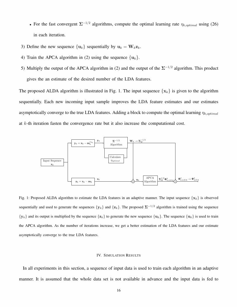
The proposed ALDA algorithm is illustrated in Fig. 1. The input sequence {xk} is given to the algorithm

sequentially. Each new incoming input sample improves the LDA feature estimates and our estimates

asymptotically converge to the true LDA features. Adding a block to compute the optimal learning ηk,optimal

at k-th iteration fasten the convergence rate but it also increase the computational cost.

Input Sequence

xk

yk = xk −mωx

k

k

zk = xk −mk

Calculateηoptimal

Σ−1/2

Algorithm

×

zk

yk

APCA

Algorithmuk

Wk → Σ−1/2W

Σ1/2W Φ

pk,LDA

×

Φpk,LDA → Φ

pLDA

Fig. 1: Proposed ALDA algorithm to estimate the LDA features in an adaptive manner. The input sequence {xk} is observed

sequentially and used to generate the sequences {yk} and {zk}. The proposed Σ−1/2 algorithm is trained using the sequence

{yk} and its output is multiplied by the sequence {zk} to generate the new sequence {uk}. The sequence {uk} is used to train

the APCA algorithm. As the number of iterations increase, we get a better estimation of the LDA features and our estimate

asymptotically converge to the true LDA features.

IV. SIMULATION RESULTS

In all experiments in this section, a sequence of input data is used to train each algorithm in an adaptive

manner. It is assumed that the whole data set is not available in advance and the input data is fed to

16

the proposed algorithms sequentially. For these simulations, MATLAB codes are run on a PC with Intel

Pentium 4, 2.6-GHZ CPU and 2048-Mb RAM.

A. Experiments on Σ−1/2algorithms

In this experiment, we first compare the convergence rate of equations (16-18) and (20-22) to estimate

the square root of the inverse covariance matrix Σ−1/2 in a ten dimensional space. The incoming input

sequence {xk} is in R10 and the covariance matrix Σ for generating the data samples is the first covariance

matrix introduced in [41] multiplied by 20. We generated 500 samples of ten dimensional, zero mean

Gaussian data with the covariance matrix Σ. The actual value of Σ−1/2 was obtained from the sample

correlation matrix using a standard eigenvector computation method. The input samples are fed to the

proposed Σ−1/2 algorithms and the algorithms are initialized to be the identity matrix, i.e. W0 = I. The

L2 norm of the error at k-th iteration between the estimated and the actual Σ−1/2 matrices is computed

by

ek =

√√√√ 10∑i=1

10∑j=1

(Wk(i, j)−Σ−1/2(i, j))2, (39)

where Wk(i, j) and Σ−1/2(i, j) represent the ij-th element of the estimated square root of the inverse

covariance matrix at k-iteration and the ij-th element of the actual square root of the inverse covariance

matrix, respectively. Fig. 2 and Fig. 3 illustrate the convergence of the proposed algorithms in (16-18) and

(20-22). From Fig. 2 it can be observed that the proposed Σ−1/2 algorithms in (16-18) have very similar

convergence rate and the convergence graphs overlap each other. The proposed algorithms in (16-18) use

an estimate of the covariance matrix and in each iteration they update this estimate using (19). As a

result, graphs in Fig. 2 show a smooth convergence to Σ−1/2. In contrast, the graphs in Fig. 3 show an

erratic behavior, since the proposed algorithms in (20-22) instead of using an estimate of the covariance

matrix use the k-th input sample to estimate the covariance matrix. Fig. 4 compares convergence rate of

algorithms in (17) and (21). Although, algorithm in (17) converges smoothly to Σ−1/2, but the convergence

rate for both algorithm is nearly the same and after 500 iterations the estimation error is negligible. It can

17

be observed from Fig. 2 and Fig. 3 that the proposed Σ−1/2 algorithms can successfully be applied for

estimation of the square root of the inverse of the covariance matrix. Since the proposed Σ−1/2 algorithms

have similar convergence rates, they can interchangeably be used to estimate Σ−1/2 in an adaptive manner.

Table I compares the normalized error resulting from the proposed Σ−1/2 algorithms in (16-18) and (20-

22) as the number of iterations changes from 100 to 500. The measurements in Table I indicate that the

estimates achieved using the proposed Σ−1/2 algorithms are close to the actual value and the estimation

errors after 500 iterations are negligible.

0 100 200 300 400 5000

0.1

0.2

0.3

0.4

0.5

0.6

0.7

0.8

0.9

1

Number of samples

Nor

mal

ized

err

or

Equation 16Equation 17Equation 18

Fig. 2: Convergence rate of the proposed Σ−1/2 algorithms in (16-18). They use the incoming input sample to update the

estimate of the covariance matrix using (19). The updated covariance matrix is used to improve the estimate of the square root

of the inverse covariance matrix. These algorithms have very similar convergence rate and overlap each other.

We also compared convergence rate of the proposed Σ−1/2 algorithm in 4, 6, 8, and 10 dimensional

spaces. For the ten dimensional space we used the same covariance matrix Σ as before (that is the first

covariance matrix in [41] multiplied by 20). The ten eigenvalues of the covariance matrix Σ in descending

18

0 100 200 300 400 5000

0.1

0.2

0.3

0.4

0.5

0.6

0.7

0.8

0.9

1

Number of samples

Nor

mal

ized

err

or

Equation 20Equation 21Equation 22

Fig. 3: Convergence rate of the proposed Σ−1/2 algorithms in (20-22). For these algorithms, only the incoming input sample

is used to find an estimate of the covariance matrix in each iteration.

order are 117.996, 55.644, 34.175, 7.873, 5.878, 1.743, 1.423, 1.213, and 1.007. The covariance matrices

for 4, 6, and 8 dimensional spaces are selected as the principal minors of Σ.The initial estimate W0 is

chosen to be the identity matrix and the proposed algorithm are trained using a sequence of Gaussian data

in each space separately. For each experiment, at k-th update, we compute the normalized error between

the estimated and the actual matrices. The convergence rate of the proposed Σ−1/2 algorithm in (22) for

each covariance matrix is illustrated in Fig. 5. It can be observed from Fig. 5 that after 500 iterations, the

normalized errors are less than 0.1 for all covariance matrices. The same experiment is repeated using

the other proposed Σ−1/2 algorithms and we got similar graphs.

In order to show the tracking ability of the introduced Σ−1/2 algorithms for non-stationary data, we

generated 500 zero mean Gaussian samples in R10with the covariance matrix as stated before. Then, We

19

0 100 200 300 400 5000

0.1

0.2

0.3

0.4

0.5

0.6

0.7

0.8

0.9

1

Number of samples

Nor

mal

ized

err

or

Equation 17Equation 21

Fig. 4: Convergence rate of algorithms (17) and (21). Although algorithm (17) converges smoothly to Σ−1/2, but both

algorithms have similar convergence rate.

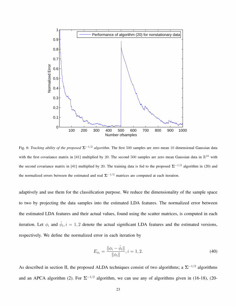
drastically changed the nature of the data sequence by generating new 500 zero mean 10-dimensional

Gaussian data with the second covariance matrix introduced in [41]. The tracking ability of the proposed

Σ−1/2 algorithm in (20) is illustrated in Fig. 6. We initiated the algorithm with W0 = I, where I is

the identity matrix. It is clear from Fig. 6 that the proposed Σ−1/2 algorithm tracks the changes in

the data. The normalized error increases when the covariance matrix alters after 500 iterations but the

algorithm gradually adapts itself to the new covariance matrix and the normalized error starts to decrease

by observing new samples from the new covariance matrix.

We show the effectiveness of the proposed accelerated Σ−1/2 algorithm to estimate Σ−1/2 by comparing

its convergence rate with the algorithm introduced in [26]. We generated 500 zero mean 10-dimensional

Gaussian data with the first covariance matrix given in [41]. The algorithm in [26] and the proposed

20

TABLE I: The normalized error for estimation of the square root of the inverse covariance matrix Σ−1/2 resulting from the proposed

equations (16-18) and (20-22), as the number of iterations increases from 100 to 500.

Number of Iteration 100 200 300 400 500

Equation (16) 0.2915 0.1545 0.1056 0.0823 0.0658

Equation (17) 0.2923 0.1558 0.1023 0.0789 0.0619

Equation (18) 0.2915 0.1545 0.1055 0.0823 0.0658

Equation (20) 0.2933 0.1461 0.0951 0.0716 0.0545

Equation (21) 0.2889 0.1467 0.0892 0.0667 0.0447

Equation (22) 0.2933 0.1462 0.0950 0.0716 0.0545

accelerated Σ−1/2 algorithm are trained using the input sequence. The optimal learning rate at k-th iteration

ηk,Optimal for the proposed algorithm is computed using (26). For the algorithm introduced in [26] a

decreasing learning rate is used. The normalized error in each iteration is computed and Fig. 7 illustrates

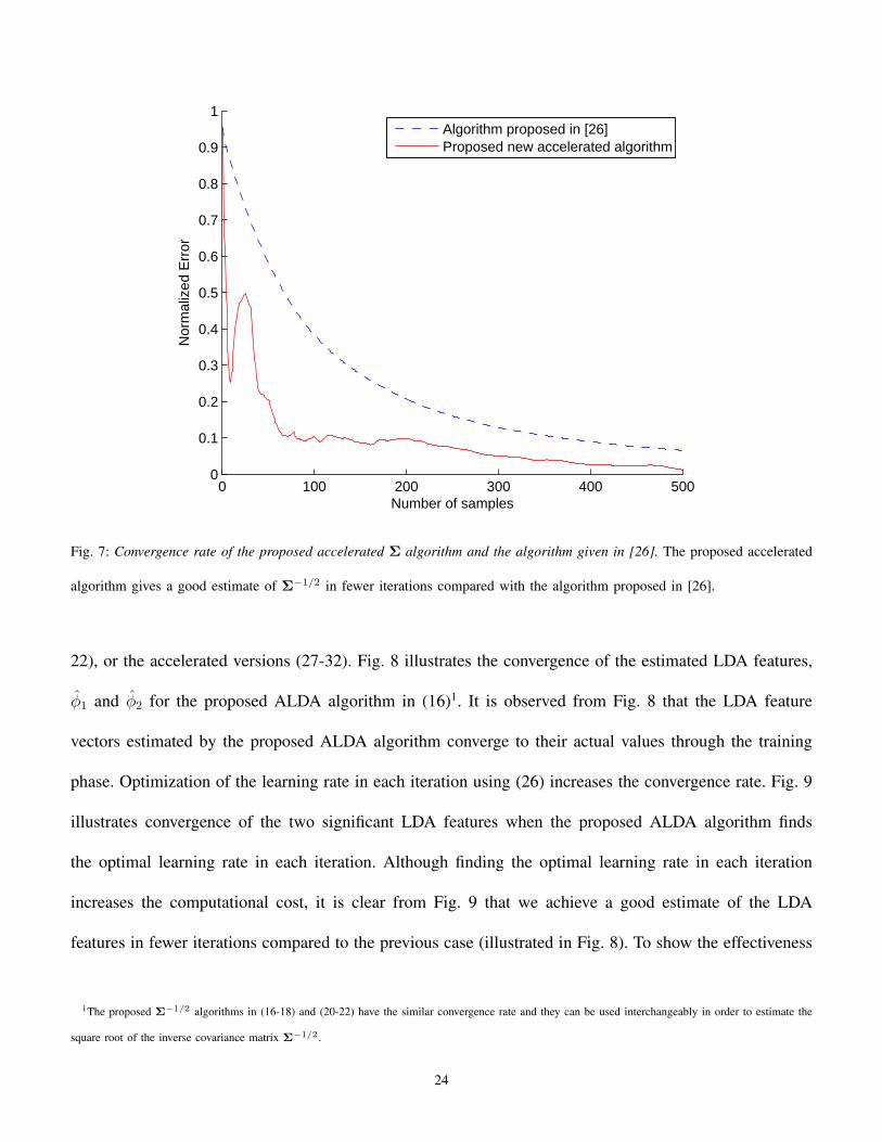
the convergence rates for these two algorithms. It can be observed from Fig. 7, the new accelerated

Σ−1/2 algorithm reaches to an estimation error of 0.1 after observing about 100 samples. In contrast, the

proposed algorithm in [26] gives an estimation error of 0.1 after training by 500 samples. This means that

by applying the new accelerated Σ−1/2 algorithm, we can achieve to the desired estimation error much

faster than using the algorithm proposed in [26].

B. Experiments on Adaptive LDA Algorithm

The performance of the proposed ALDA algorithms are tested using i) ten dimensional, five class

Gaussian data, ii) four dimensional, three class Iris data set, and iii) five class, 40 × 40 gray scale face

images.

21

0 100 200 300 400 5000

0.1

0.2

0.3

0.4

0.5

0.6

0.7

0.8

0.9

1

Number of samples

Nor

mal

ized

err

or

d=10d=8d=6d=4

Fig. 5: Convergence rate of the proposed algorithms. We used algorithm in (22) to estimate Σ−1/2 in 4, 6, 8, and 10

dimensional spaces. For simulation in 10 dimensional space, we used the first covariance matrix in [41] and multiplied it

by 20. The covariance matrices for the lower dimensions are chosen as the principal minors of the covariance matrix in 10

dimensional space.

1) Experiment on ten dimensional data: We test the performance of the proposed ALDA algorithm to extract

the significant LDA features 1 adaptively. We generated 500 samples of 10-dimensional Gaussian data for

each of five classes with different mean value and covariance matrices, i.e. 2500 samples in total. The

means and the covariance matrices are obtained from [41] with the covariance matrices multiplied by 20.

The eigenvalues of Σ−1W ΣB in descending order are 10.84, 7.01, 0.98, 0.34, 0, 0, 0, 0, 0, and 0. Thus, the

data has intrinsic dimensionality of four and only two features corresponding to the eigenvalues 10.84 and

7.01 are significant. We use the proposed ALDA algorithms to estimate the two significant LDA features

1By significant LDA features, we mean directions that are the most important for the class separability purpose. These directions are the eigenvectors of

Σ−1W ΣB corresponding to the largest eigenvalues.

22

100 200 300 400 500 600 700 800 900 10000

0.1

0.2

0.3

0.4

0.5

0.6

0.7

0.8

0.9

1

Number ofsamples

Nor

mal

ized

Err

or

Performance of algorithm (20) for nonstationary data

Fig. 6: Tracking ability of the proposed Σ−1/2 algorithm. The first 500 samples are zero mean 10 dimensional Gaussian data

with the first covariance matrix in [41] multiplied by 20. The second 500 samples are zero mean Gaussian data in R10 with

the second covariance matrix in [41] multiplied by 20. The training data is fed to the proposed Σ−1/2 algorithm in (20) and

the normalized errors between the estimated and real Σ−1/2 matrices are computed at each iteration.

adaptively and use them for the classification purpose. We reduce the dimensionality of the sample space

to two by projecting the data samples into the estimated LDA features. The normalized error between

the estimated LDA features and their actual values, found using the scatter matrices, is computed in each

iteration. Let ϕi and ϕi, i = 1, 2 denote the actual significant LDA features and the estimated versions,

respectively. We define the normalized error in each iteration by

Eϕi=

∥ϕi − ϕi∥∥ϕi∥

, i = 1, 2. (40)

As described in section II, the proposed ALDA techniques consist of two algorithms; a Σ−1/2 algorithms

and an APCA algorithm (2). For Σ−1/2 algorithm, we can use any of algorithms given in (16-18), (20-

23

0 100 200 300 400 5000

0.1

0.2

0.3

0.4

0.5

0.6

0.7

0.8

0.9

1

Number of samples

Nor

mal

ized

Err

or

Algorithm proposed in [26]Proposed new accelerated algorithm

Fig. 7: Convergence rate of the proposed accelerated Σ algorithm and the algorithm given in [26]. The proposed accelerated

algorithm gives a good estimate of Σ−1/2 in fewer iterations compared with the algorithm proposed in [26].

22), or the accelerated versions (27-32). Fig. 8 illustrates the convergence of the estimated LDA features,

ϕ1 and ϕ2 for the proposed ALDA algorithm in (16)1. It is observed from Fig. 8 that the LDA feature

vectors estimated by the proposed ALDA algorithm converge to their actual values through the training

phase. Optimization of the learning rate in each iteration using (26) increases the convergence rate. Fig. 9

illustrates convergence of the two significant LDA features when the proposed ALDA algorithm finds

the optimal learning rate in each iteration. Although finding the optimal learning rate in each iteration

increases the computational cost, it is clear from Fig. 9 that we achieve a good estimate of the LDA

features in fewer iterations compared to the previous case (illustrated in Fig. 8). To show the effectiveness

1The proposed Σ−1/2 algorithms in (16-18) and (20-22) have the similar convergence rate and they can be used interchangeably in order to estimate the

square root of the inverse covariance matrix Σ−1/2.

24

0 500 1000 1500 2000 25000

0.1

0.2

0.3

0.4

0.5

0.6

0.7

0.8

0.9

1

Number of samples

Nor

mal

ized

Err

or

First LDA featureSecond LDA feature

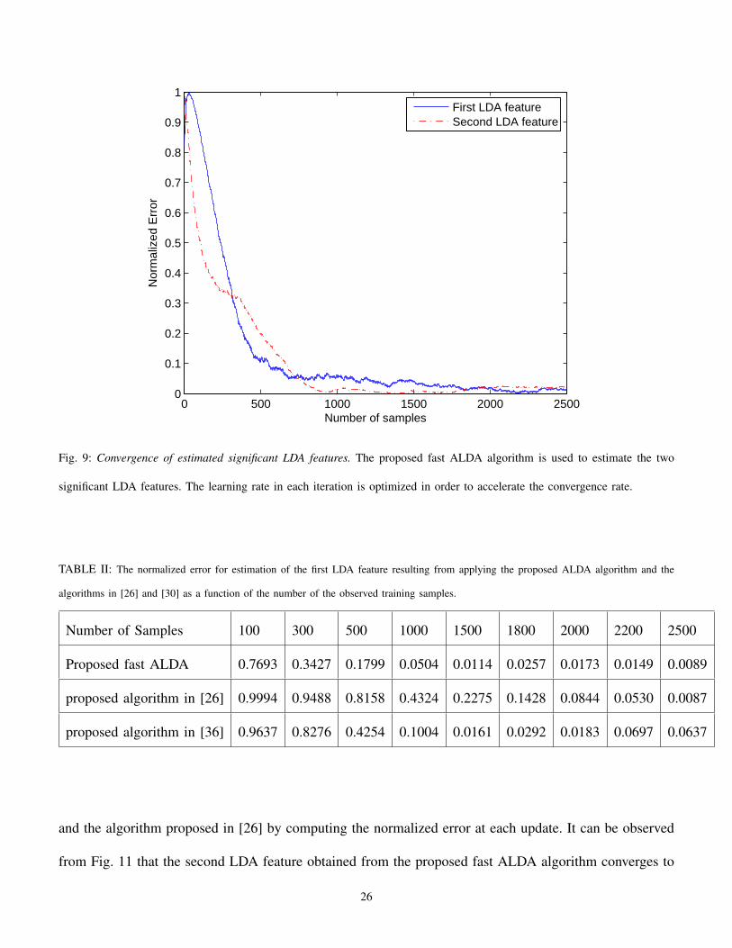
Fig. 8: Convergence of estimated significant LDA features. In this simulation, the proposed ALDA algorithm uses Σ−1/2

algorithm in (16) in order to estimate Σ−1/2W .

of the proposed fast ALDA algorithm 1, we compare its performance to estimate the first LDA feature with

the techniques introduced in [26] and [30]. The normalized error as a function of the number of samples

is shown in Fig. 10 for these three algorithms. It is clear from Fig. 10, the proposed fast ALDA algorithm

gives a better estimate of the LDA feature in fewer iteration compared to the proposed algorithms in [26]

and [30]. Table II compares the normalized error for the estimation of the first LDA feature resulting

from applying the proposed algorithm and the algorithms introduced in [26] and [30], respectively, as

a function of the number of the observed training samples. It is clear from Table II, the proposed fast

ALDA algorithm outperforms the algorithms in [26] and [30] in term of the convergence rate.

In Fig. 11, We show the convergence of the second LDA feature using the proposed fast ALDA algorithm

1By fast ALDA algorithm we mean the ALDA algorithm that compute the optimal learning rate using (26) in each iteration in order to accelerate the

convergence rate.

25

0 500 1000 1500 2000 25000

0.1

0.2

0.3

0.4

0.5

0.6

0.7

0.8

0.9

1

Number of samples

Nor

mal

ized

Err

or

First LDA featureSecond LDA feature

Fig. 9: Convergence of estimated significant LDA features. The proposed fast ALDA algorithm is used to estimate the two

significant LDA features. The learning rate in each iteration is optimized in order to accelerate the convergence rate.

TABLE II: The normalized error for estimation of the first LDA feature resulting from applying the proposed ALDA algorithm and the

algorithms in [26] and [30] as a function of the number of the observed training samples.

Number of Samples 100 300 500 1000 1500 1800 2000 2200 2500

Proposed fast ALDA 0.7693 0.3427 0.1799 0.0504 0.0114 0.0257 0.0173 0.0149 0.0089

proposed algorithm in [26] 0.9994 0.9488 0.8158 0.4324 0.2275 0.1428 0.0844 0.0530 0.0087

proposed algorithm in [36] 0.9637 0.8276 0.4254 0.1004 0.0161 0.0292 0.0183 0.0697 0.0637

and the algorithm proposed in [26] by computing the normalized error at each update. It can be observed

from Fig. 11 that the second LDA feature obtained from the proposed fast ALDA algorithm converges to

26

0 500 1000 1500 2000 25000

0.1

0.2

0.3

0.4

0.5

0.6

0.7

0.8

0.9

1

Number of Samples

Nor

mal

ized

Err

or

Algorithm introduced [26]New proposed Accelerated algorithmAlgorithm introduced in [30]

Fig. 10: Convergence of the estimated first LDA feature. Convergence rate of the proposed fast ALDA algorithm to estimate

the first significant LDA feature is compared with that of the algorithms introduced in [26] and [30].

its true value faster than the algorithm introduced in [26]1. We project the training data on the subspace

spanned by the estimated LDA features ϕ1 and ϕ2 in order to show the effectiveness of the proposed ALDA

algorithm to find directions for the maximum class separability. Fig. 12 demonstrates the distribution of

the input data on the subspace spanned by the estimated two significant LDA feature vectors resulting

after 500, 1000, 1500, and 2500 iterations. From Fig. 12, it can be observed that when the number of

iterations increases, the distributions of the five classes on the estimated LDA feature subspace become

more separable. As the number of the iterations increases, we get a more precise estimate of the significant

LDA features and the projected data points start to be classified into five separable clusters. We can observe

1Since the proposed algorithm in [30] does not have the capability of estimating the desired number of LDA features simultaneously, we compared the

convergence rate of the proposed algorithm to estimate the second significant LDA feature with the algorithm introduced in [26]. The algorithm in [30]

estimates the LDA features sequentially, it first estimates the most significant LDA feature and then uses it to estimate the second significant LDA feature

and this procedure continues to estimate the rest of LDA features.

27

0 500 1000 1500 2000 25000

0.1

0.2

0.3

0.4

0.5

0.6

0.7

0.8

0.9

1

Number of Samples

Nor

mal

ized

Err

or

Algorithm introduced in [26]Proposed accelerated algorithm

Fig. 11: Convergence of the estimated second LDA feature. Convergence rate of the proposed fast ALDA algorithm to estimate

the second LDA feature is compared with that of the algorithm introduced in [26].

from Fig. 12, after 500 iterations we have a poor estimate of the significant LDA features and fives classes

in the estimated subspace mix together. However, when gradually the number of iterations increase, the

classes start to separate from each other and finally after 2500 iterations they are linearly separable in

the estimated LDA feature subspace1. Although four LDA features are necessary for the complete class

separation2, Fig. 12 shows that the projection onto the subspace spanned by two significant LDA features

separate the data into five classes.

2) Experiment with Iris data set: The Iris flower data set 3 is a well-known, multivariate data set that has been

widely used as a non-synthetic data to evaluate classification techniques [42] [43]. This data set consists of

50 samples from each of three species of Iris flowers including Iris setosa, Iris virginica, and Iris versicolor.

1There are some overlappings and they are not perfectly linearly separable.2As mentioned earlier, the ten dimensional matrix Σ−1

W ΣB used in this experiment has only four nonzero eigenvalues.3The data set is available at http://archive.ics.uci.edu/ml/machine-learning-databases/iris/

28

−10 −5 0 5 10−10

−5

0

5

10After 2500 iterations

first class second class third class fourth class fifth class

−5 0 5−5

0

5After 500 iterations

−5 0 5 10−5

0

5After 1000 iterations

−10 −5 0 5 10−10

−5

0

5After 1500 iterations

Fig. 12: Distribution of the input data in the estimated LDA subspace. The input data is projected into the subspace spanned by

the two significant LDA features estimated using the proposed ALDA algorithm. Increasing the number of iterations improve

the estimate of the LDA features and five classes become more separable.

Four features were measured in centimeters from each sample. The measured features are the length and

the width of sepal and petal [44]. One class is linearly separable from the other two classes, the latter

are not linearly separable from each other. The eigenvalues of Σ−1W ΣB in descending order are 32.7467,

1.2682, 0.9866, and 0.9866. Although the data set has intrinsic dimensionality of four for the classification,

only one feature is significant. The first eigenvalue of Σ−1W ΣB, that is 32.7467, greatly dominates others.

Therefore, is clear that almost all the necessary information for the class separability lies on the direction

of the eigenvector corresponding to the largest eigenvalue and the rest of the eigenvectors do not play

29

0 50 100 1500

0.1

0.2

0.3

0.4

0.5

0.6

0.7

0.8

0.9

1

Number of samples

Nor

mal

ized

Err

or

First LDA featureSecond LDA feature

Fig. 13: Convergence of two significant LDA features for the Iris data set. The proposed ALDA algorithm is applied to the

Iris data set in order to estimate two significant LDA features. It can be observed that the normalized error after 150 iterations

is negligible.

an important role for the classification purpose. To get a better visual representation of the data samples

in the feature space, we estimate two significant LDA features (LDA feature vectors corresponding to

32.7467 and 1.2682) and project the four dimensional data onto the subspace spanned by the estimated

features. In order to achieve a fast convergence, we used the proposed accelerated Σ−1/2 algorithm. The

data samples are fed to the proposed ALDA algorithm sequentially and the LDA features are estimated in

an adaptive manner. Fig. 13 illustrates convergence of two significant LDA features as a function of the

number of the training samples. We project the four dimensional samples onto the estimated significant

LDA features. Fig. 14 shows distribution of the Iris data set in the subspace spanned by the estimated

two significant LDA features. It can be observed from Fig. 14 that the data samples distributed linearly

30

4 5 6 7 8 9 10 112.5

3

3.5

4

4.5

5

5.5

6

First LDA feature

Sec

ond

LDA

feat

ure

SetosaVersicolorVirginica

Fig. 14: Distribution of the Iris data set in the subspace spanned by the estimated LDA features. The four dimensional samples

of the Iris data set are projected onto the subspace spanned by the LDA features estimated using the proposed ALDA algorithm.

To get a better understanding of the distribution of data samples in the estimated subspace, we did projection onto the two

significant LDA features. The first class, Iris Setosa, is linearly separable from other classes, the two remaining classes overlap

each other.

in the estimated two dimensional LDA subspace, that confirms using just the first significant LDA feature

would be enough for the classification.

3) Experiment on the Yale face data base B: To test the performance of the proposed ALDA algorithm to

extract the significant LDA features, we applied it to the Yale face data base B. The Yale face data base

B contains 5760 single light source images of 10 subjects each seen under 576 viewing conditions (9

poses × 64 illumination conditions) [45]1. We selected 5 individual subjects and considered 64 images

1The Yale face data base B can be accessed online at urlhttp://cvc.yale.edu/projects/yalefacesB/yalefacesB.html

31

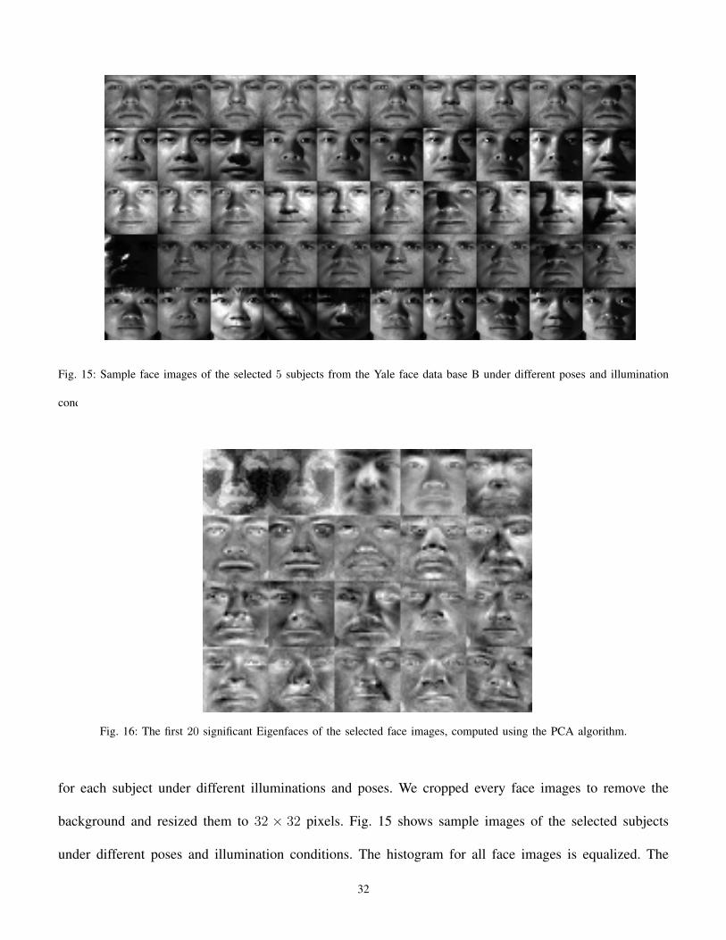
Fig. 15: Sample face images of the selected 5 subjects from the Yale face data base B under different poses and illumination

conditions.

Fig. 16: The first 20 significant Eigenfaces of the selected face images, computed using the PCA algorithm.

for each subject under different illuminations and poses. We cropped every face images to remove the

background and resized them to 32 × 32 pixels. Fig. 15 shows sample images of the selected subjects

under different poses and illumination conditions. The histogram for all face images is equalized. The

32

0 50 100 150 200 250 3000

0.1

0.2

0.3

0.4

0.5

0.6

0.7

0.8

0.9

1

Number of Samples

Nor

mal

ized

Err

or

ALDA Algorithm in (16)APCA Algorithm in (2)

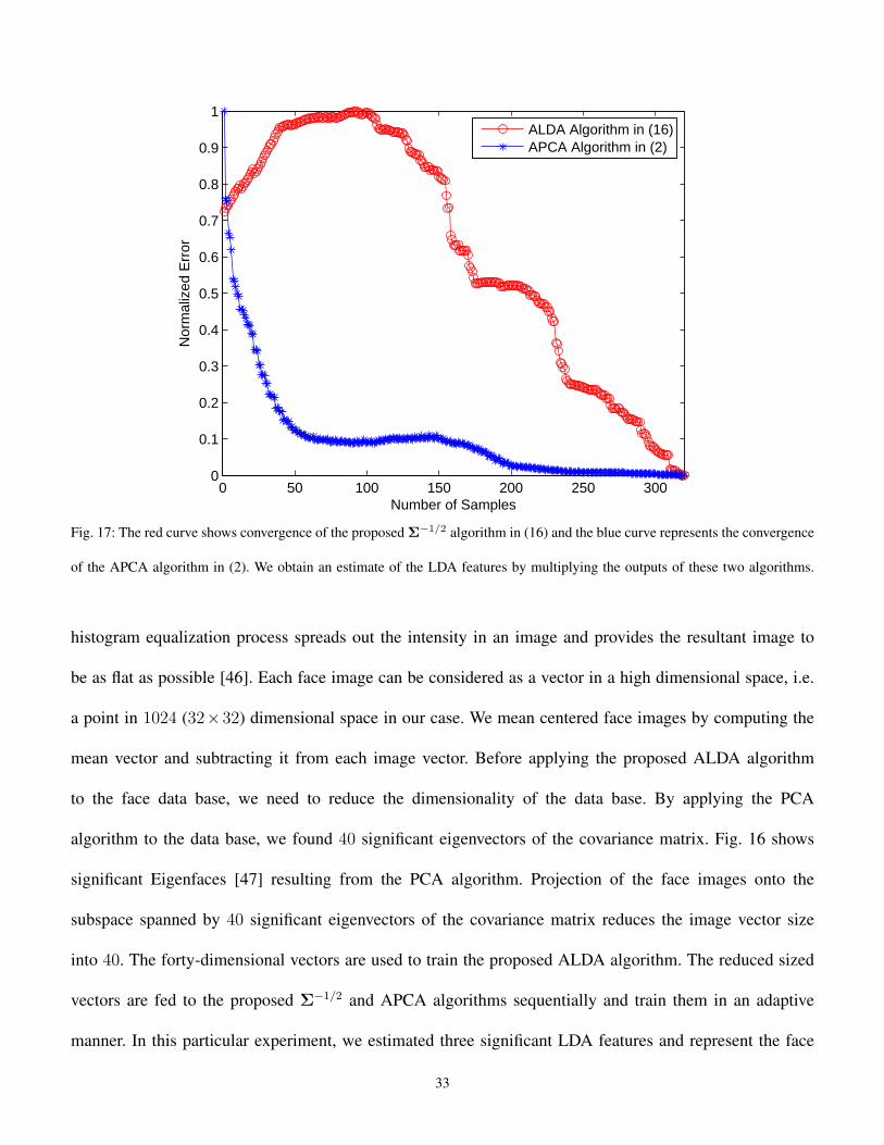
Fig. 17: The red curve shows convergence of the proposed Σ−1/2 algorithm in (16) and the blue curve represents the convergence

of the APCA algorithm in (2). We obtain an estimate of the LDA features by multiplying the outputs of these two algorithms.

histogram equalization process spreads out the intensity in an image and provides the resultant image to

be as flat as possible [46]. Each face image can be considered as a vector in a high dimensional space, i.e.

a point in 1024 (32×32) dimensional space in our case. We mean centered face images by computing the

mean vector and subtracting it from each image vector. Before applying the proposed ALDA algorithm

to the face data base, we need to reduce the dimensionality of the data base. By applying the PCA

algorithm to the data base, we found 40 significant eigenvectors of the covariance matrix. Fig. 16 shows

significant Eigenfaces [47] resulting from the PCA algorithm. Projection of the face images onto the

subspace spanned by 40 significant eigenvectors of the covariance matrix reduces the image vector size

into 40. The forty-dimensional vectors are used to train the proposed ALDA algorithm. The reduced sized

vectors are fed to the proposed Σ−1/2 and APCA algorithms sequentially and train them in an adaptive

manner. In this particular experiment, we estimated three significant LDA features and represent the face

33

−500

50

−100

10−10

0

10

After 50 iterations

−500

50

−200

20−5

0

5

After 150 iterations

−500

50

−200

20−10

0

10

After 200 iterations

−500

50

−200

20−20

0

20

After 320 iterations

First Class Second Class Third Class Fourth Class Fifith Class

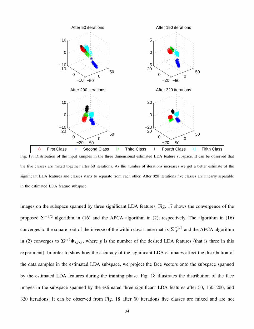
Fig. 18: Distribution of the input samples in the three dimensional estimated LDA feature subspace. It can be observed that

the five classes are mixed together after 50 iterations. As the number of iterations increases we get a better estimate of the

significant LDA features and classes starts to separate from each other. After 320 iterations five classes are linearly separable

in the estimated LDA feature subspace.

images on the subspace spanned by three significant LDA features. Fig. 17 shows the convergence of the

proposed Σ−1/2 algorithm in (16) and the APCA algorithm in (2), respectively. The algorithm in (16)

converges to the square root of the inverse of the within covariance matrix Σ−1/2W and the APCA algorithm

in (2) converges to Σ1/2ΦpLDA, where p is the number of the desired LDA features (that is three in this

experiment). In order to show how the accuracy of the significant LDA estimates affect the distribution of

the data samples in the estimated LDA subspace, we project the face vectors onto the subspace spanned

by the estimated LDA features during the training phase. Fig. 18 illustrates the distribution of the face

images in the subspace spanned by the estimated three significant LDA features after 50, 150, 200, and

320 iterations. It can be observed from Fig. 18 after 50 iterations five classes are mixed and are not

34

linearly separable. By observing new samples and improving the estimate of the LDA features, classes

start to separate from each other. As the number of iterations increase, the amount of overlapping between

classes reduces and after 320 iterations five classes are almost linearly separable.

V. CONCLUSION

In this paper, we presented new adaptive algorithms to estimate the square root of the inverse covariance

matrix Σ−1/2. The proposed algorithms are derived by optimization of an appropriate cost function that is

introduced for the first time. The optimal learning rate in each iteration is computed in order to accelerate

the convergence rate of the proposed Σ−1/2 algorithms. We used the output of Σ−1/2 algorithm to construct

a new training sequence for an APCA algorithm. It has been shown that the product of the outputs of

the APCA algorithm and Σ−1/2 algorithm converges to the desired LDA features. The convergence rate

of the proposed accelerated ALDA algorithms to estimate the LDA features is compared with that of the

current algorithms. The simulation results indicate that the proposed accelerated ALDA algorithms give

an accurate estimate of the LDA features in fewer iterations compared with that of the current algorithms.

Furthermore, existence of the cost function makes it possible evaluate the accuracy of the estimates

obtained by using different initial conditions and learning rates. A sequence of the input data is used to

train the ALDA algorithms in an adaptive manner. The adaptive nature of the proposed ALDA algorithms

makes them appropriate for online applications such as mobile robotic or online face recognition. The

proposed Σ−1/2 algorithms require to start from a symmetric and positive definite matrix that commutes

with the covariance matrix. This is the only constraint that needs to be satisfied in order to guaranty

the convergence of the proposed algorithms. The constraint on the initial condition can be satisfied by

choosing the initial estimate W0 to be the identity matrix. Note that, the proposed ALDA algorithms

have limitations of the LDA method. They give us at most K − 1 features, where K is the number of

classes. Therefore for applications that more features are needed, some other methods must be employed

to provide additional features. Similar to the LDA method, the proposed ALDA algorithms implicitly

35

assume Gaussian distribution for the available classes. If the distributions are significantly non-Gaussian,

the LDA features may not be useful for the classification purpose. The proposed ALDA algorithms are

tested on the real world data set with the small number of classes (four classes for the Iris data set and

five classes for the Yale face data base B). It is obvious that when the number of classes increases they

may not be linearly separable. In this case we have to use nonlinear techniques such as neural networks

for the classification of the data samples. Design and training a neural network with many input can be

complicated and time consuming. The proposed ALDA algorithm can be used as a preprocessing step

to reduce the dimensionality of the input data. Then the outputs of the ALDA algorithm, that lie on an

lower dimensional subspace spanned by the LDA features, are fed into a neural network for the nonlinear

classification task.

APPENDIX A

We prove the following lemma for the cost function J(W) defined in (10),

Lemma 1. Let Σ be the covariance matrix of the input samples. Let S denote the set of all symmetric

and positive definite matrices W that commute with the square root of the covariance matrix, i.e., S =

{W : |Wt = W,xtWx > 0, for all non-zero x ∈ Rn, and WΣ1/2 = Σ1/2W}. Then the cost function

J(W) : S → R is a convex function and its global minimum occurs at W = Σ−1/2.

Proof: If the positive definite and symmetric matrix W commutes with the square root of the

covariance matrix, i.e. WΣ1/2 = Σ1/2W, then we have

WΣ = WΣ1/2Σ1/2 = Σ1/2WΣ1/2 = Σ1/2Σ1/2W = ΣW. (A.1)

That means the matrix W commutes also with the covariance matrix Σ, i.e. WΣ = ΣW. From equation

(9), we have

J(W) =1

3tr[(WΣ1/2 − I)2(W + 2Σ−1/2)]

=1

3tr[(WΣ1/2WΣ1/2 − 2WΣ1/2 + I)(W + 2Σ−1/2)]. (A.2)

36

Using the commutative property between W and Σ, we can simplify (A.2) as follows

J(W) =1

3tr[(W2Σ− 2WΣ1/2 + I)(W + 2Σ−1/2)]

=1

3tr[W3Σ+ 2W2Σ1/2 − 2W2Σ1/2 − 4W +W + 2Σ−1/2]

=1

3tr[W3Σ+ 2Σ−1/2 − 3W]

=1

3tr(W3Σ) +

2

3tr(Σ−1/2)− tr(W). (A.3)

The first derivative of the cost function J(W) with respect to W is given by

∂J(W)

∂W=

ΣW2 +WΣW +ΣW2

3− I

= ΣW2 − I, (A.4)

For the last equality, we used the commutation property given in (A.1). Equating the first derivative of

the cost function J(W) to zero, we get W = Σ−1/2. Hence, W = Σ−1/2 is the only stationary point of

the cost function J(W). The product of two positive definite matrices is also a positive definite matrix

and we have the same property for the trace of a positive definite matrix. Therefore, the cost function in

(9), that is trace of the product of two positive definite matrices, is a positive definite matrix and we have

J(W) ≥ 0. The cost function J(W) at the stationary point W = Σ−1/2 is zero, therefore Σ−1/2 is the

only global minimum of the cost function. An alternative way to show that the stationary point Σ−1/2 is

a global minimum of the cost function J(W) is using the following theorem [38]

Theorem 1. A real valued, twice differentiable function J : S → R defined on an open convex set S is

convex if and only if its Hessian matrix is positive semi-definite.

The Hessian matrix of the cost function J(W) is given by

H(J(W)) = Σ⊗W +ΣW ⊗ I, (A.5)

where I is the identity matrix and ⊗ denote the Kronecker product. Since W and Σ are positive definite

matrices and commute, then their product also is a positive definite matrix [38]. The Kronecker product

37

of two positive definite matrices is also a positive definite matrix, therefore the Hessian matrix H given

in (A.5) is also a positive definite matrix. Using theorem 1 the cost function J(W) is a convex function

and W = Σ−1/2 is a absolute minimum of the cost function.

APPENDIX B

The cost function J(W) at k + 1-th iteration is given be

J(Wk+1) =tr(W3

k+1Σ)

3− tr(Wk+1) +

2

3tr(Σ−1/2). (B.1)

The estimate at k + 1-th iteration is computed using the following adaptive algorithm

Wk+1 = Wk + ηk(I−WkΣWk). (B.2)

Let Gk = I−WkΣWk. Introducing Gk into (B.1) and using A.1 yields,

J(Wk+1) =tr((Wk + ηkGk)

3Σ)

3− tr(Wk + ηkGk) +

2

3tr(Σ−1/2)

=tr(W3

kΣ+ 3ηkW2kGkΣ+ 3η2kWkG

2kΣ+ η3kG

3kΣ)

3− tr(Wk + ηkGk) +

2

3tr(Σ−1/2).

(B.3)

We take derivative of the cost function in B.3 with respect to the learning rate and equate it to zero in

order to find the optimal learning rate. We obtain

∂J(Wk+1)

∂Wk+1

= tr(W2kGkΣ) + 2ηktr(WkG

2kΣ)− tr(Gk) + η2ktr(G

3kΣ)

= ck + bkηk + akη2k, (B.4)

where ak = tr(G3kΣ), bk = 2tr(WkG

2kΣ), and ck = tr(W2

kGkΣ)− tr(Gk).

APPENDIX C

Lemma 2. Let xk ∈ Rn, k = 1, 2, . . . represent the input samples. Let mk be the total mean estimate

at k-th iteration. Let mωxkk denote the estimate of the sample mean of the class that xk belongs to it at

k-th iteration. Let the sequence {y}k=1,2,... defined by yk = xk −mωxkk Define the sequence {zk}k=1,2,...

to be zk = xk −mk. Let the sequence {uk}k=1,2,... defined by uk = Wkzk, where Wk is the output of a

38

Σ−1/2 algorithm trained by the sequence {yk}. Then the correlation of the sequence {yk} as k goes to

infinity converges to the within-class scatter matrix ΣW . Furthermore, limit of the correlation matrix for

the sequence {uk} converges to Σ−1/2W ΣΣ

−1/2W .

Proof: We first prove that the correlation of the sequence {yk} converges to the within-class scatter

matrix as k goes to infinite. The limit of the correlation matrix of the sequence {yk} is computed as

follows

limk→∞

ykytk = lim

k→∞E[(xk −m

ωxkk )(xk −m

ωxkk )t]

= E[(xk −mωxk )(xk −mωxk )t]

=K∑i=1

P (ωi)E[(xk −mωxk )(xk −mωxk )t|ωxk= ωi]

=K∑i=1

P (ωi)Σωi

= ΣW , (C.1)

where K is the number of available classes, ωii = 1, . . . , K denote the i-th class, and Σωi denote the

covariance matrix for the class ωi.

The correlation matrix for the sequence {uk} is computed as follows

limk→∞

ukutk = lim

k→∞E[Wk(xk −mk)(xk −mt

kWtk]

= E[Σ−1/2W (x−m)(x−m)t(Σ

−1/2W )t]

= Σ−1/2W E[(x−m)(x−m)t](Σ

−1/2W )t

= Σ−1/2W ΣΣ

−1/2W . (C.2)

REFERENCES

[1] K. Fukunaga, Introduction to Statistical Pattern Recognition, 2nd Edition, Academic Press, New York, 1990.

39

[2] L. Chen, H. M. Liao, M. Ko, J. Lin,G. Yu, “New LDA based face recognition system which can solve the small sample size problem,” Pattern Recognition,

vol. 33, no. 10, pp. 1713-1726, 2000.

[3] J. Lu, K. N. Platantinos, A. N. Venetsanopoulos, “Face recognition using LDA-based algorithms,” IEEE Trans. Neural Networks, vol. 14, no. 1, pp.

195-200, 2003.

[4] H. Yu,J. Yang, “A direct LDA algorithm for high-dimensional data with application to face recognition,” Pattern Recognition, vol. 34, no. 10, pp.

2067-2070, 2001.

[5] Y. Koren, L. Carmel, “Visualization of labeled data using linear transformation,” in Proc. the Ninth IEEE conf. on Information visualization, pp. 121-128,

Oct. 2003.

[6] C. Chang, H. Ren, “An Experimented-based quantitative and comparative analysis of target detection and image classification algorithms for hyper-spectral

imagery,” IEEE Trans. Geoscience and Remote Sensing, vol. 38, no. 2, pp. 1044-1063, 2000.

[7] C. C. Aggarwal, J. Han, J. Wang, P. S. Yu, “On demand classification of data streams,” in Proc. ACM SIGKDD Int. Conf. Knowledge discovery data

mining, pp. 503-508, Aug. 2004.

[8] D. L. Swets, J. J. Weng, “Using Discriminant eigen-feature for image retrieval,” IEEE Trans. Pattern Analysis and Machine Intelliigence, vol. 18, no.

8, pp. 831-836, 1996.

[9] W. Zhao, R. Chellappa, A. Krishnaswamy, “Discriminant analysis of principal components for face recognition,” in Proc. IEEE Int. Conf. on Automatic

face and gesture recognition, Nara, Japan, pp. 336-341, 1998.

[10] P. N. Belhumeur, J. P. Hespanha, D. J. Kriegman, “Eigen-faces vs. Fisher-faces: Recognition using class specific linear projection,” IEEE Trans. Pattern

Analysis and Machine Intelligence, vol. 19, pp. 711-720, 1997.

[11] A. M. Martinez, A. C. Kak, “PCA versus LDA,” IEEE Trans. Pattern Analysis and Machine Intelligence, vol. 23, no. 2, pp.228-233, 2001.

[12] P. Hall, A. D. Marshall, R. Martin, “Incremental eigen analysis for classification,” in Proc. Brit. Machine Vision Conf., vol. 1, pp. 286-295, 1998.

[13] P. Hall, A. D. Marshal, R. Martin, “Merging and splitting eigen space models,” IEEE Trans. Pattern Analysis and Machine Intelligence, vol. 22, no. 9,

pp. 1042-1049, 2000.

[14] Y. Miao, Y. Hua, “Fast subspace tracking and neural network learning by a novel information criterion,” IEEE Trans. Signal Processing, vol. 46, pp.

1964-1979, 1998.

[15] S. Bannour, M. R. Azimi-Sadjadi, “Principal component extraction using recursive least squares learning,” IEEE Trans. Neural Network, vol. 6, pp.

457-469, 1995.

[16] L. Xu, “Least mean square error reconstruction principle for self-organizing neural-net,” Neural Networks, vol. 6, pp. 627-648, 1993.

[17] J. Weng, Y. Zhang, W. S. Hwang, “Candid covariance free incremental principal component analysis” IEEE Trans. Pattern Analysis and Machine

Intelligence, vol. 25, no. 8, pp 1034-1040, Aug. 2003.

[18] E. Oja, j. Karhunen, “On stochastic approximation of eigenvectors and eigen-values of the expectation of a random matrix,” Journal of Mathematical

Analysis and Applications, vol. 106, pp. 69-84, 1990.

[19] E. Oja, “Principal components, minor components, and linear neural networks,” Neural Networks, vol.5, pp. 927-935, 1992.

[20] T. D. Sanger, “Optimal unsupervised learning in a single-layer linear feed forward neural network,” Neural Networks, vol. 2, pp. 459-473, 1989.

[21] C. Chatetrjee, A. Kang, V. Roychodhury, “Algorithms for Accelerated Convergence of Adaptive PCA,” IEEE Trans. on Neural Networks, vol. 11, no.

2, pp. 338-355, 2000.

[22] S. Pang, S. Ozawa, N. Kasabov, “Incremental linear discriminant analysis for classification of data streams,” IEEE Trans. on System, Man and Cybernetics-

Part B, vol. 35, no. 5, pp. 905-914, 2005.

40

[23] T. Kim, S. Wong, B. Stenger, J. Kittler, R. Cipolla, “Incremental Linear Discriminant Analysis Using Sufficient Spanning Set Approximation,” in Proc.

IEEE Int. Conf. Computer Vision and Pattern Recognition (CVPR), pp. 1-8, June 2007.

[24] J. Ye, Q. Li, H. Xiong, H. Park, R. Janardan, V. Kumar, “IDR/QR: An incremental dimension reduction algorithm via QR decomposition,” IEEE Trans.

on Knowledge and Data Engineering, vol. 17, no. 9, 2005.

[25] J. Mao, A.K. Jain, “Discriminant analysis neural networks,” in Proc. IEEE Int. Conf. on Neural Networks, CA, pp. 300-305, 1993.

[26] C. Chatterjee, V. P. Roychowdhurry, “On self-organizing algorithm and networks for class separability features,” IEEE Trans. Neural Network, vol. 8,

no. 3, pp. 663-678, 1997.

[27] G.K. Demir, K. Ozmehmet, ”On-line local learning algorithm for linear discriminant analysis,” Pattern Recognition Letters, vol. 26, pp. 421-431, 2005.

[28] H. Abrishami Moghaddam, M. Matinfar, S. M. Sajad Sadough, K. Amiri Zadeh, “Algorithms and networks for accelerated convergence of adaptive

LDA,” Pattern Recognition, vol. 38, no. 4, pp. 473-483, 2005.

[29] H. Abrishami Moghaddam, M. Matinfar, “Fast adaptive LDA using quasi-Newton algorithm,” Pattern Recognition Letters, vol. 28, no. 4, pp. 613-621,

2007.

[30] Y. Rao, N. Principe, J. C. Wong, “Fast RLS like algorithm for generalized eigen decomposition and its applications,” Journal of VLSI Signal processing

systems, vol. 37, no. 3, pp. 333-344, 2004.

[31] Y. Aliyari Ghassabeh, H. Abrishami Moghaddam, “Adaptive algorithms and networks for optimal feature extraction from Gaussian data,” Pattern

Recognition Letters, vol. 31, pp. 1331-1341, Aug. 2010.

[32] H. Hongo, N. Yasumoto, Y. Niva, K. Yamamoto, “Hierarchical face recognition using an adaptive discriminant space,” in Proc. IEEE Int. Conf. Computers

Communications, Control and Power Engineering (TENCON), vol. 1, pp. 523-528, 2002.

[33] S. Ozawa, S. L. Toh, S. Abe, S. Pang, N. Kasabov, “Incremental learning of feature space and classifier for face recognition,” Neural Networks, vol. 18,

pp. 575-584, 2005.

[34] S. Theodoridis, Pattern Recognition. 2nd Edition, Academic Press, New York, 2003.

[35] M. Woelfel, J. McDonough, Distant Speech Recognition. Wiley, 2009.

[36] L. Ljung, “Analysis of recursive stochastic algorithms,” IEEE Trans. Automatic Control, vol. 22, pp. 551-575, 1977.

[37] K. Diamantaras, S. Kung, Principal Component Neural Networks, Theory and Applications. Wiley, New York, 1996.

[38] J. R. Magnus, H. Neudecker, Matrix Differential Calculus. John Wiley, 1999.

[39] H. J. Kushner, D. S. Clarck, Stochastic approximation methods for constrained and unconstrained systems Springer-Verlag, New York, 1978.

[40] A. Benveniste, M. Metivier, P. Priouret, Adaptive algorithms and stochastic approximations. 2nd Edition, Academic Press, New York, 1990.

[41] T. Okada, S. Tomita, “An optimal orthonormal system for discriminant analysis,” Pattern Recognition, vol. 18, no.2, pp. 139-144, 1985.

[42] E. R. Hruschka, N. F. Ebecken,“Extracting rules from multilayer perceptrons in classification problems: A clustering-based approach,” Neurocomputing,

vol. 70, pp. 384397, Dec. 2006.

[43] C. H. Wang, Y. Y, Chi, “Dynamic Optimal Training of A Three Layer Neural Network with Sigmoid Function,” in Proc. IEEE int. conf. on Networking,

Sensing and Control, Fort Lauderdale, USA, pp. 392-397, Aug. 2006.

[44] http://en.wikipedia.org/wiki/Iris flower data set

[45] A. S. Georghiades, P. N. Belhumeur, D. J. Kriegman, “From Few to Many: Illumination Cone Models for Face Recognition under Variable Lighting

and Pose,” IEEE Trans. Pattern Analysis and Machine Intelligence, vol. 23, no. 6, pp/ 643-660, Jun. 2001.

[46] N. Rajkumar, S. Vijayakumar, C. Murukesh, “Intellectually combined face recognition using curvelet based principle component analysis for feature

41

extraction and Bayesian Classifier,” in Proc. IEEE int. conf. on Signal Processing, Communication, Computing and Networking Technologies (ICSCCN),

Chennai, India, pp. 374-378, Sep. 2011.

[47] M. Turk, A. Pentland, “Eigenfaces for face recognition,” Journal Cognitive Neuroscience, vol. 3, no.1, pp 71-86, 1991.

42