ALADIN NEWSLETTER 27 - umr-cnrm.fr

ALADINNEWSLETTER 27

July-December 2004

Copyright: ©ALADIN 2005 1

Scientific Editor: Dominique GIARDLinguistic Advisor & Lay out: Jean-Antoine MAZIEJEWSKIWeb Master: Patricia POTTIER & Jean-Daniel GRIL

1This paper has only a very limited circulation and permission to quote from it should be obtained from the CNRM/GMAP/ALADIN

2

ALADIN Newsletter 271. EDITORIAL

Experience has shown that the rather strict deadlines fixed last summer (22/07 and 22/01)were too stringent. Many papers, including mandatory ones (reports on operations and research foreach centre), cannot be ready in time. And some papers sent, suffer from hasty writing, bringingeven more work to the editorial team.

As a consequence, the next deadlines will be fixed for the end July and the end of Januaryrespectively, there are nicest ways to celebrate JAM's birthday! And please, do use the (updated)style sheets and proof read your contribution before sending them to the editorial team (JAM andDG).

A new tool, made for openoffice, which you can use to write equations and formulæ can befound on: http://www.dmaths.com/

1.1. EVENTS

1.1.1. 26th EWGLAM and 11th SRNWP meetingsThe annual joint EWGLAM and SRNWP meetings were organized by met.no, on 4-7 October

2004, in Oslo (Norway). Most presentations and the minutes are available on the SRNWP web site :http://srnwp.cscs.ch/, and the LAM Newsletter should be available soon.

During the SRNWP meeting, the decision to propose "now" a Marie Curie Research TrainingNetwork was taken (voted). This led to the STORMNET project. More details in the ALADIN-2section.

The minutes of the many informal ALADIN meetings and discussions along this week, withseveral strategic issues debated, are available at : http://www.cnrm.meteo.fr/aladin/meetings/informal.html#2004

1.1.2. 9th Assembly of ALADIN PartnersThis extended Assembly, with several scientists and two HIRLAM representatives present,

was held close to Split (Croatia), on 30-31 October 2004. It had to deal with 3 major issues :- the ALADIN-HIRLAM cooperation, welcomed by all Directors,

- the preparation of the next Memorandum of Understanding, with the nomination of a workinggroup and some preliminary input,

- a partial change of priorities within the ALADIN-2 short-term plan.The minutes (thanks to Maria Derkova) and the presentations are available on the ALADIN

web site, at: http://www.cnrm.meteo.fr/aladin/meetings/minutesass9.html. Do have a look at them !

1.1.3. TCWGPDI workshopThe TCWGPDI (Training Course and Working Group on Physical/Dynamical Interfacing)

was held in Prague from the 22d till the 26th of November 2004. Around 40 participants from theALADIN, HIRLAM, ARPEGE-IFS and AROME communities gathered together. The aim of theworkshop was twofold : firstly, a training course and secondly, to define the basis of futurecommon physical/dynamical interface for the several physics of the different communities listedabove.

3

The training course was really fruitful with a complete review on the basic equations(considering a multiphase air parcel) and stability aspects, a state of the art of the ideas around theorganisation of the time-step and some links with the dynamical part (non-hydrostatic aspects).

The second goal was not reached. However, the talk enabled to get some informations on theconstraints imposed by the different physics and also on the way some already implementedsolutions were done (AROME prototype, IFS surface scheme).

1.1.4. HIRLAM-ALADIN mini-workshop on convection and cloud processesThis was the first joint workshop, a HIRLAM initiative. It was organized in the framework of

the "Nordic Network on Fine-scale Atmosperic Modelling" in Tartu (Estonia), on 24-26 January2005. Presentations are available at : http://hirlam.fmi.fi/CCWS/

This workshop was a real success, with around 30 participants representing the HIRLAM,ALADIN-2 (all declinations), COSMO, Meso-NH, MM5, MC2, ... worlds. Working groups allowedvery constructive discussions, especially on the physics-dynamics interface (esp. the definition ofimplementation rules common to all HIRLAM and ALADIN-2 options) and the grey-zone problem,with the emergence of a new approach, considering the complementarity between the variousparameterizations rather than between resolved and unresolved contributions.

1.1.5. Other workshopsJoint HIRLAM-SRNWP workshop on "Surface Processes and Assimilation"Held on 15-17 September 2004, in Norrköping (Sweden). The report presented by Stefan

GOLLVIK at the 11th SRNWP meeting is available on the SRNWP web site.

LAM-EPS days in ViennaOrganized by ZAMG on 25-28 October 2004.

Joint HIRLAM-SRNWP workshop on "High resolution data assimilation: towards 1-4kmresolution"

Held on 15-17 November 2004, in Exeter (UK), with very many participants. More details at :http://www.metoffice.gov.uk/research/nwp/external/srnwp/workshop_nov2004/index.html

SRNWP workshop on "Numerical Techniques"Practically included in the ECMWF seminar on "Recent developments in numerical methods

for atmosphere and ocean modelling", 6-10 September, Reading (UK).

1.1.6. Other eventsTwo bad news : Günther Doms, the father of the Local Model and a leader of the COSMO

group, and Patrick Jabouille, an expert in Meso-NH physics and one of the first members of theAROME team, died during Summer.

New directors in 2004 or early 2005 : in Tunisia, Croatia, Morocco and Hungary.

1.2. ANNOUNCEMENTS

1.2.1. HIRLAM All Staff Meeting

To be held on March 14-16, 2005, in Dublin (Ireland).Unfortunately, there will be only French ALADIN representatives. The HIRLAM research

plan for the next years, especially mesoscale challenges, will be discussed.

4

1.2.2. 2nd SRNWP workshop on "Short-Range Ensemble Prediction Systems"To be organized on April 7-8, 2005, in Bologna (Italy), by the Ufficio Generale per la

Meteorologia.The workshop will be arranged on selected talks covering :

- global prediction systems and evaluation techniques, - ensemble prediction systems for short range, - related international projects.

There will be a session dedicated to the discussion on the following selected topics:- methodologies for initial perturbations in limited-area models and interactions with boundaries - model perturbations; parameters settings, stochastic physics- how to combine properly different models (and different analysis) in a different model approach ?- ensemble data assimilation: feasible for limited-area models ?- ensemble size- validation techniques

More details at : http://www.meteoam.it/

1.2.3. 4th WMO international symposium on "Assimilation of Observations in Meteorologyand Oceanography"

To be held on April 18-22, 2005, in Prague (Czech R.).This will be a huge meeting, with up to 270 participants registered. And this will be an

opportunity for ALADIN and HIRLAM scientists to discuss research plans for the next years. More details on the program at : http://www.chmi.cz/dasympos/index.html

1.2.4. ICAM-MAP meetingThe 28th International Conference on Alpine Meteorology (ICAM) and the Annual Scientific

Meeting of the Mesoscale Alpine Programme (MAP) 2005 will take place in ZADAR (Croatia),from Monday 23 to Friday 27, May 2005.

The conference will be hosted by the Meteorological and Hydrological Service of Croatia, the"Andrija Mohorovi" Geophysical Institute (University of Zagreb) and the Croatian MeteorologicalSociety. ALADIN contributions are welcome !

Local Organizing Committee ICAM/MAP2005: e-mail: [email protected](lien à faire vers ICAM pdf)

1.2.5. LM Users seminarThe Deutscher Wetterdienst (DWD) will be holding a seminar on the design, products and

operational use of the NWP model-chain of the DWD in Langen (Germany) from the 30th of May tothe 3rd of June 2005.. Non-COSMO participants are also welcome.

Contact: Dr Wilfried Jacobs [email protected]

1.2.6. 3rd SRNWP workshop on "Statistical and Dynamical Adaptation"To be held on June 1-3, 2005, in Vienna (Austria), at the Central Institute for Meteorology

and Geodynamics (ZAMG). As in previous years, presentations on all aspects of statistical and physical/dynamical

adaptation in numerical weather prediction are welcome. Contributions about adaptation of EPSproducts, in particular with regard to extreme events, are particularly welcome.

A web page has been set up for the 3rd SRNWP Workshop on Statistical and Dynamical

5

Adaptation. Please visit http://www.zamg.ac.at/swsa2005/ You can use the on-line form to register,and to make a hotel reservation.

If you intend to give a presentation, send a short abstract to [email protected] (until31 March 2005).

For questions regarding accommodation please contact [email protected]

1.2.7. 15th ALADIN workshop "QUO VADIS, ALADIN ?"To be organized in June 6-10, 2005, in Bratislava (Slovakia), by SHMI (contact points : Maria

Derkova and Michal Majek). Web site: www.shmu.sk. The workshop venue is the SUZA CongressCenter (www.suza.sk).

The workshop is intended to review the current status and ongoing developments ofmesoscale modelling and to enable the exchange of information and ideas inside the meteorologicalcommunity. Those can cover wide range of research results in the fields of model dynamics, physicsand data assimilation, including ensemble predictions. Contributions focussing on 2-3km targetscales will be of particular interest. Presentations on local applications, technical and operationalenvironment, verifications are also welcome. The poster session shall be devoted mainly to thestatus of your operational applications.

And, most important, this workshop should deliver the next medium-term research plan forALADIN (2005-2008).

1.2.8. And next ...• HIRLAM workshop on mesoscale modelling (physics mainly ?)

September 2005 - Norway

• 27th EWGLAM & 12th SRNWP meetings3-6 October, 2005 – Ljubljana, Slovenia

• SRNWP workshop on non-hydrostatic modelling31 October - 2 November, 2005 - Bad Orb, Germany

• 10th Assembly of ALADIN partnersOctober 21, 2005 - Bratislava, Slovakia

• HIRLAM-ALADIN working week on variational data assimilation ?An informal proposal from Per Unden ...

• Next ALADIN-HIRLAM training courseNovember 2005 ? - Bucarest, RomaniaMore details in the ALADIN-2 section

1.3. ALADIN 2

1.3.1. IntroductionThis section is dedicated to the project's life. Up to now, contributions were only French ones,

but this must change. So don't hesitate to send input next time !

6

1.3.2. A closer ALADIN-HIRLAM cooperationThe "code collaboration" between the ALADIN and HIRLAM consortia did start, officially

and practically.

At the 9th Assembly of Partners (30-31 October), ALADIN directors welcomed the HIRLAMproposal, presented by the chairperson of the HIRLAM Advisory Committee and the ProjectLeader, of a closer "code" collaboration (i.e. towards the use of a common model allowing historicalspecificities for all operational applications). The following resolution was adopted, and presentedto the HIRLAM Council on December 15th by Dr Ivan CACIC. HIRLAM directors gave a verypositive answer.

Resolution on ALADIN-HIRLAM cooperation Adopted by the ALADIN General Assembly on 30 October 2004

The ALADIN General Assembly, meeting in Split, Croatia, on 29-30 October 2004:Considering the common goal of HIRLAM and ALADIN to develop, implement and maintain

operational NWP systems at the meso-gamma scale, while maintaining state-of-the art meso-betaoperational capabilities, based on their respective scientific, technical and managerial heritage;

Considering the proposal of the HIRLAM Council for cooperation with ALADIN, based oncode collaboration and scientific exchange;

Noting that cooperation with HIRLAM should be consistent and compatible with theALADIN high level objectives, strategy and short term plans, in particular the priority assigned to:

- the continuing development of a meso-beta model improving the current operationalcapabilities available to ALADIN partners, capitalising on the ALADIN scientific andtechnical heritage and new agreed concepts;

- its necessary and timely convergence with the parallel development of the AROME meso-gamma model, based on the ALADIN data assimilation and core dynamics, and the Meso-NH physics;

Stressing the importance of the guidelines for relations among National Meteorological orHydrometeorological Services regarding commercial activities attached as Annex 2 to the WMOResolution 40 (Cg XII), that aim at maintaining and strengthening in the public interest thecooperative and supportive relations among NMSs in the face of differing national approaches tothe growth of commercial meteorological activities;

1- Welcomes the decision of the HIRLAM Council to explore full code cooperation withALADIN and appreciates the relevance of the preparatory work performed by ALADIN andHIRLAM scientists;

2- Agrees that an efficient cooperation based on code collaboration, leading ultimately to acommon library available for use by meso-beta and meso-gamma scale NWP models, wouldbe beneficial to both HIRLAM and ALADIN, in particular, but not exclusively, in areasincluding the following: - Extended use of the ALADIN core dynamics;

7

- Data assimilation techniques and assimilation of high resolution, remotely sensedobservations from radars, satellites, etc.;

- Limited area model ensemble prediction systems (LAMEPS); - Mesoscale-oriented physics; - Boundary conditions and coupling at high resolution; - Training.

3- Considers that operational complexity needs to be minimised and efficiency maintainedthrough the adoption of a common code maintenance approach based on best practices acrossthe IFS/ARPEGE/ALADIN/HIRLAM chain, and taking into account the HIRLAM needsrelated to their near-real time Reference Control Run;

4- Agrees that efficient joint arrangements should be established without delay at science andproject levels, aimed at defining consistent scientific strategies and short term work plans,including common elements to be agreed by HIRLAM and ALADIN;

5- Supports, and proposes to HIRLAM, the following approach: - The ALADIN Committee for Scientific and Strategic Issues (CSSI) and the HIRLAM

Management Group (HMG), should establish, on behalf of the ALADIN and HIRLAMscientists and relevant bodies, a joint science plan addressing common issues, that wouldbecome part of the respective ALADIN and HIRLAM science plans;

- The ALADIN Workshop and the HIRLAM All Staff Meeting should derive and propose acommon annual work plan consistent with this joint science plan and with maintenanceconstraints, that would become part and parcel of their respective work plans;

- The HIRLAM and ALADIN/AROME project management should approve this commonwork plan, taking into account committed resources and agreed priorities, and capitalisingon the work of the respective advisory bodies.

- This process should be consolidated by July 2005. 6- Agrees to further investigate the details of the cooperation, including political and legal

aspects, in the context of the preparation of the next ALADIN and HIRLAM respectiveMemorandums of Understanding, with the objective of agreeing the articles permitting theHIRLAM-ALADIN cooperation.

7- Agrees in this regard that appropriate reference to the guidelines for relations among NationalMeteorological or Hydrometeorological and Meteorological Services (NMSs) regardingcommercial activities, attached to the WMO Resolution 40 (Cg XII), should be included in thenext ALADIN and HIRLAM MoUs.

8- Notwithstanding the above, concurs with the views of HIRLAM that, subject to appropriatecooperation agreements: - Both consortia would share ownership for commonly developed code; - Ownership of pre-existing codes would not be transferred; - All members of each Consortium would have rights to use shared software/common

libraries for their operational and research activities; - All members of each Consortium would have rights to make available research versions of

shared software to their national research communities, for exclusive research and educationpurposes.

9. Proposes that HIRLAM and ALADIN should have observer status at the ALADIN GeneralAssembly and the HIRLAM Council, respectively, in order to facilitate communication andcommon understanding.

As concerns common actions, the following ones started along the last months, beside the

8

previous cooperations :- training of the "mesoscale" group on ALADIN environment, - implementation of the HIRALD setup at ECMWF and first experiments, with the help of theFrench team (see the dedicated paper), - coupling HIRLAM physics with ALADIN dynamics, contribution to the discussions on the rulesfor physics-dynamics interfacing.

Cooperations on the following issues have also been or should be launched soon : use offrames, penta-diagonal semi-implicit operator, implementation of configurations 923 and 901 atECMWF. They won't involve only the French team.

1.3.3. STORMNET✗ Introduction

During the dedicated SRNWP session of the last annual EWGLAM/SRNWP meetings, it wasdecided to answer the first coming (deadline December 2nd, 2004) call for proposals of ResearchTraining Networks within the Marie Curie actions of the 6th Framework Program of the EC. In caseof failure, since this call was restricted to "Interdisciplinary and Intersectorial" projects, a secondattempt should be possible, in September 2005.

Thanks to intense networking and the efficient help of the SRNWP coordinator, Jean Quiby,we managed to prepare everything in time. This proposal relies on the fruitful ALATNETexperience, but with an enlarged basis : SRNWP cooperation, with 16 participants from allconsortia, wider training and research program, and a more decentralized management.

Hereafter is the "identity card" of the project, more informations are available on theSTORMNET web site : http://www.cnrm.meteo.fr/stormnet/ , the first SPIP web site of PatriciaPottier. And thanks to Claude Fischer for the name !

✗ DescriptionTitle : STORMNET (Scientific Training for Operations and Research in a Meteorological

NETwork), a European training network for local short-range high-resolution numerical weatherprediction and its applications

Short abstract :European meteorological services now have to face the challenge of a quick march towards

very high resolution applications for limited-area modelling and short-range prediction. Beside theresearch work specific to numerical weather prediction, the increased complexity of equations andthe huge amount of data to handle at a reasonable cost will raise new problems in numerics andcode organization. The positive feedback on downstream applications like hydrology or air-pollution modelling will have to be checked too. As experts are spread among many small teams, anenhanced transfer of knowledge through training actions is needed.

Full Partners :Meteo-France / National Meteorological Research Centre, Central Institut for Meteorology and Geodynamics (Austria), Royal Meteorological Institute of Belgium, Meteorological and Hydrological Service of the Republic of Croatia, Czech Hydro-Meteorological Institute, Finnish Meteorological Institute, German Weather Service, Hungarian Meteorological Service, Irish Meteorological Service, Royal Netherlands Meteorological Institute, Norwegian Meteorological Institute,

9

National Meteorological Administration (Romania), Slovak Hydro-Meteorological Institute, Swedish Meteorological and Hydrological Institute, Federal Office of Meteorology and Climatology (MeteoSwiss), Met Office of United Kingdom.

Associated Partners :University of Zagreb (Andrija Mohorovicic Geophysical Institute, Faculty of Science) (Hr), National Scientific Research Centre (Laboratoire d' Aérologie, Observatoire Midi-Pyrénées) (Fr), University College Dublin (Ir), Comenius University (Faculty of Mathematics, Physics and Informatics, Department of Astronomy,Geophysics and Meteorology) (Sk), Swiss Federal Institute of Technology Zurich (Institute of Geodesy and Photogrammetry) (Ch).

1.3.4. Coordination✗ A second life for CSSI

The CSSI (Committee for Scientific and Strategic Issues) structure, a coordination team of 6persons nominated by the Assembly of Partners (Doina Banciu, Radmila Brozkova, Luc Gérard,Dominique Giard, Andras Horanyi, Abdallah Mokssit), has been more or less shelved whenlaunching the ALADIN-2 project.

Since HIRLAM is a very structured project, the Assembly of Partners decided to both pushforward and renew CSSI, in order to make it a mirror of the HIRLAM Management Group. Thecomposition was changed, to better take into account the contributions of the various partners : 2LACE members, 2 French ones and 2 "non-LACE non-French" ones. Luc Gérard and AbdallahMokssit resigned, while Margarida Belo Pereira and Gwenaëlle Hello entered the group. AndrasHoranyi was proposed as chairperson by Directors, and the other members agreed.

However, one has to underline that this is a temporary organization, waiting for the new MoU.Proposals for a better coordination structure are welcome and should be addressed to AndrasHoranyi, who represents scientists within the working group in charge of the new MoU. ✗ Coordination of operational activities

First let's recall that Maria Derkova (Mariska) is responsible for the coordination of theupdates of operational suites, with the help of the Toulouse Support Team.

The first step, moving to the most recent export version (cycle 28T3), should be achievedsoon (see the section on operations). Some further actions have already been identified : - coordination around the conception of observation databases, with several partners willing to startdata assimilation activities or to update the present tools; CHMI and HMS already providedinformations on how to proceed; ANM, NIMH and DMN are likely to organize a working groupwith joint stays in Toulouse;- many modifications in coupling files scheduled for summer 2005, with a coordinated operationalchange expected for September;- jump to the externalized surface module in 2006. 1.3.5. The misfortunes of the ALARO-10 sub-project, arguments around the physics-dynamics interface, ...

As underlined in Oslo (in October), "this was a difficult year indeed", and the last months of2004 were even worse, with sharp arguments and again a lack of visibility after re-re-formulationsof objectives. The new targets are described in the mail sento all teams by Jean-François Geleyn onthe 4th of February, 2005.

10

1.3.6. Communication problems, obviouslyThere were complains from ALADIN Partners about the multiple voices of Météo-France, and

they were justified indeed, with a poor diffusion of information and significant disagreementswithin the French team, hence less attention paid to the Partners' opinions.

As an attempt to restart on safer bases, a meeting was organized in Toulouse on January 19th,2005, with representatives of the various models used at Météo-France. Hereafter are the minutes,written by Jean Pailleux, who is now responsible for coordination at the CNRM level.

Météo-France meeting of 19 January 2005 on LAM NWP (ALADIN, ALARO, AROME, MESO-NH)

The meeting was organised by the Météo-France Research management in Toulouse,involving the Direction Générale in Paris (A. Ratier, C. Blondin) and the Forecasting service (E.LEGRAND). It was triggered by:

- the Prague workshop (22-26 November 2004) which failed to establish a satisfying work-plan,especially for the ALADIN-2 project, and especially in terms of physics-dynamics interface;

- several email exchanges taking place between the Prague workshop and the end of 2004, whichwere pointing to an insufficient level of coordination between the different LAM projects(ALARO, AROME, etc...) which have been all set up with heavy contraints on their time-tables.Among the different weaknesses which were identified before and during this meeting, one is

the fact that the ALARO prototype has been developed in 2004 in a software environment which isas close as possible to the AROME prototype. As this AROME software environment is aprovisional one, which is not expected to converge to its final environment before 2008 (and is quitefar from the operational environment which is familiar to the ALADIN world), this is a stronglimitation for the scientists working on the ALADIN-2 who have to prepare ALARO runs.

Following a planning effort by Jean-François Geleyn just before the 19 January meeting, a listof critical scientific/technical tasks was identified in terms of work-streams (rather than in terms ofALARO project or AROME project). These tasks were then analysed in order to identify theminimum which needs to be achieved for the ALARO project and its time-table. The followingpoints are coming out from the meeting:

- The intermediate calendar of ALARO is relaxed, i.e. no big phasing effort in 2005, but morepreparation for a 2006 upgrade, to happen after the technical change to the externalised surfacecode and files, planned before mid-2006 (see specific plan by D. Giard, on the ALADIN web).For end 2006, the aim is now a first version of ALARO which would be an improvedALADIN, still preserving further "re-convergence" with AROME.

- A guess of the first version of the ALARO physics can be seen as follows: the use of asophisticated micro-physics package is postponed and will be revisited in the context of theconvection closure; the convection scheme is a modified version of ARPEGE/ALADIN; idemfor the gravity wave drag; the radiation code is a simplified and cheap version of RRTM; use ofthe externalised surface (which is then the first technical jump to the ALARO code, beforemid-2006). The new physical routines called in this context should be callable from the Meso-NH side as well as the ALARO side (so-called "symmetric compatibility"). This first version ofthe ALARO physics is based on pragmatic considerations which have nothing to do with thequality of existing models, or the performance of Meso-NH physics at 10km.

- Most of the coordination problems between ALARO and AROME are now concentrated in theroutine APLAROME calling both the AROME and ALARO parameterization routines(APLAROME routine renamed APLXX – see separate short-term plan written by FrançoisBouttier on the ALADIN web).

11

- Some rules on the evolution of the Meso-NH code have now been suggested (document byFrançois Bouttier– see ALADIN web). They are of the same type as the rules used for years inIFS – ARPEGE – ALADIN. They should be the guarantee that each LAM project can rely onall the other projects in terms of code, in a way which is flexible enough. Each project isexpected to benefit from all the others in a symmetric way.

- The "generalised interface of interfaces" is not cancelled, but in its more ambitious form it ispostponed , say beyond 2008. It is currently not compatible with the ALARO and AROMEcalendars, although it is potentially a very powerful tool for research in NWP and climatemodelling.

1.3.7. Fourth medium-term research planWe have now to build the fourth ALADIN medium-term research plan, for years 2005-2008.

The third one was valid till end 2004 only, though prolongated for 6 months by a provisional workplan. The target is to build a first draft with contributions from all partners before the next ALADINworkshop (June), then discuss and finalize it there. Common issues with the parallel HIRLAMresearch plan will be identified during a preliminary CSSI-HMG meeting on Sunday just before theworkshop.

A convivial web site for the preparation of the research plan was created by Patricia Pottier : http://www.cnrm.meteo.fr/aladin/wp2005-2008/

So, please :- do have a look at the site !- do contribute to discussions !- do travel to Bratislava in June (financial support is available) !

1.3.8. Support✗ Next ALADIN training course

Considering the needs expressed by the ALADIN teams (all answered !) and the candidacies,it was decided to organize an ALADIN-HIRLAM training course :- in Bucarest (in the brand new school), - at the end of 2005, November as far as possible, because of the numerous meetings before, - on the following topics : Meso-NH physics, running the AROME prototype, use of NH dynamics.✗ Documentation

The most recent version of ARPEGE-ALADIN documentation is now available via theALADIN web site. The next step is the definition of a web site dedicated to documentation. PatriciaPottier and Jean-Marc Audoin are in charge of it in Toulouse. ✗ MAE supported projects : AMADEUS, ECONET-SELAM

A proposal for bilateral cooperation between Austria and France (AMADEUS) for 2005-2006was accepted. Coordinators : Eric Bazile and Yong Wang.

A proposal for support to a network involving Bulgaria, Romania, Macedonia, Moldavia, andFrance, for 2005-2006, was submitted in December. Two main issues are considered : training anddesign of observation databases. It was not accepted, unluckily (around 200 proposals weresubmitted). ✗ Météo-France financial support

Support to participation to workshops ("KIT") is available for 2005, as last year. Hoping therewill be less problems !

Support to stays in Toulouse, mainly for maintenance and training actions, was accepted forthe same amount as last year.

12

1.4. GOSSIP

Practical English Le français Pratique

To carry a torch for someone Avoir un faible pour quelqu'unTo get on like a house on fire S'entendre à merveilleTo look daggers at someone Foudroyer quelqu'un du regardTo let one's hair down Se détendreTo paint the town red Faire la fêteTo be out on the tiles Sortir faire la bringueTo be on cloud nine Être aux angesTo be down in the mouth Être dépriméTo be in the doldrums Avoir le moral à zéroTo go off at the deep end Piquer une criseTo go ballistic Piquer une criseTo be at the end of one's tether Être à boutTo be like a bear with a sore head Être d'humeur massacranteTo haul someone over the coals Démolir quelqu'un en le critiquantThe pot calling the kettle back L'hôpital qui se moque de la charitéTo pick holes in something Relever des erreurs dans quelque choseTo get a rollicking Se faire engueulerTo have someone's guts for garters Massacrer quelqu'unTo brick it Avoir les jetonsTo get the wind up Avoir une peur bleueTo be in bed with someone Être allié avec quelqu'un de façon officieuseTo stick one's oar in Mettre son grain de selTo sell someone down the river Trahir/vendre quelqu'unTo be long in the tooth Ne plus être tout jeuneTo be up the pole Être timbréTo bend over backward Se mettre en quatreTo give someone a leg up Donner un coup de pouce à quelqu'unTo pull somebody's leg Faire marcher quelqu'unTo look like death warmed up Avoir une mine de déterréTo laugh all the way to the bank S'en mettre plain les pochesTo cost an arm and a leg Coûter les yeux de la têteTo push the boat out Ne pas regarder à la dépenseTo go Dutch Payer chacun sa partTo take someone to the cleaners Plumer quelqu'unTo wet one's whistle Se rincer le gosierOn a wing and a prayer Dieu sait commentTo go out on a limb Prendre des risquesTo be in a rut Être enlisé dans la routineIt's a different kettle of fish C'est une autre affaireTo be like chalk and cheese C'est le jour et la nuitThe penny's dropped Çà y est! J'ai comprisTo put out feelers Tâter le terrainTo hear something on the grapevine Apprendre quelque chose par le téléphone arabeTo hear something from the horse's mouth Apprendre quelque chose de source sûreTo grasp the nettle Prendre le taureau par les cornesTo shoot the breeze BavarderTo bend someone's ear Pomper l'air à quelqu'un

13

To talk through one's hat Parler à tord et à traversTo be all mouth and no trousers Être une grande gueuleTo bust a gut Se donner un mal de chienTo go through the mill En baverA hard nut to crack Un problème difficile à résoudreA hot potato Un sujet délicatTo play the field PapillonnerTo have been left on the shelf En passe de devenir vieille filleTo go up the wall Se fâcher tout rouge

Some books I read and what I thought of them.The diary of Thomas Turner 1754-1765: edited by David Vaisey.

This diary chronicles the daily life of a Sussex shopkeeper in mid-eighteenth century. It beginin 1754 , Thomas Turner then aged 25, and end on the eve of his second marriage. Besides being amultipurpose shopkeeper, Thomas Turner was also a pillar of the community for, for many years, hewas either parish officer, churchwarden, overseer of the poor, surveyor of the highway or collectorof the window and land taxes.

Well written, it is worth reading as it gives an inside glimpse of the life of ordinary men andwomen, the hardship for a shopkeeper to get its money, the trading practices of the time, the afterChristmas revelling, eating and much drinking, quarrelling with an obstreperous wife and mother inlaw, and much more besides, in short with life and death.

The Wench is dead :Colin DEXTERA century old whodunit brilliantly solved by bed ridden Chief Inspector Morse recovering at

the JR2 from a perforated ulcer and amid tantalizing nurses and for a one night bed fellow LowlandSister.

Morse suspects foul play, when, back in the 1850s, three boat men are convicted then hangedfor the murder of Joanna Frank, despite their claim to innocence. After much thinking and a nil bymouth diet, Morse proceeds to unravel the swindle enacted by Joanna Frank and her con-manhusband.

Julia de Roubigné: Henry McKenzieJulia and destitute Savillon are brought up together by Julia's parents, and, years later and

unknown to each other, they fall in love. Then, Savillon leaves France for Martinique to join a richchildless relative.

In the meantime, Julia's father goes near bankrupt and unexpectedly, Julia's mother dies.Julia's is compelled to marry M. Montauban, a rich neighbour who paid the young woman's haughtyfather's debts. Lack of communication between husband and wife together with Julia'ssentimentality daydreaming about her faraway bosom friend leads to sudden jealousy fromMontauban deludes himself of being wronged and then proceeds to poison his young wife and tocommit suicide

This epistolary novel, written by the the author of the most famed Man of feeling is moreconcerned with the unruly feelings of the protagonists than with plot. Best left to oblivion, though,one will find a nice passage against slavery, well in advance of its time. In a way, Julia de Roubignéprefigures the novels of, say, Henry James.

The diary of a Cotswold ParsonA biased selection of what must have otherwise been an interesting account of early

nineteenth century life. To be read by those interested by landscape, countryside and architecture,otherwise, can be happily discarded.

Lor' luv a duck!

14

2. OPERATIONS

2.1. An overview of operational ALADIN applications January 2005

2.1.1. Model characteristics

PartnerModel

x (km)

L t(s)

GridpointsC+I / C+I+E

Grid type SW corner(lat , lon)

NE corner(lat , lon)

Coupling model

AUSTRIA 9.6 45 415 289 × 259300 × 270

quadratic 33.99N, 2.17E 55.62N, 39.07E ARPEGE

BELGIUMBE

7.0 41 300 229 × 229240 × 240

linear 43.17N, 5.84W 57.25N, 17.08E ALADIN- FRANCEARPEGE

BULGARIABG

12.0 41 514 79 × 6390 × 72


CROATIALACE

12.2 37 514 229 × 205240 × 216


CROATIAHRn8

8.0 37 327 169 × 149180 × 160

quadratic 39.00N, 5.25E 49.57N, 22.30E ALADIN-LACE

CROATIADyn Adap (6)

2.0 15 60 72 × 72 80 × 80

Senj, Karlovac, Maslenica,Split, Dubrovnik,Osijek

ALADIN-HRn8

CZECH R.CE

9.0 43 360 309 × 277320 × 288

linear 33.99N, 2.18E 55.62N, 39.08E ARPEGE

FRANCE 9.5 41 415 289 × 289300 × 300

linear 33.14N, 11.84W 56.96N, 25.07E ARPEGE

HUNGARYHU

6.5 37 270 421 × 373432 × 384


HUNGARYDyn Adap

2.4 15 239 × 169250 × 180

ALADIN-HU

MOROCCONORAF

31 37 900 189 × 289200 × 300

quadratic 1.93S, 35.35W 44.86N, 57.22E ARPEGE

MOROCCOALBACHIR

16.7 37 675 169 × 169180 × 180

quadratic 18.13N, 19.99W 43.11N, 9.98E ALADIN-NORAF

POLAND 13.5 31 169 × 169180 × 180


PORTUGAL 12.7 31 600 79 × 89 90 × 100

quadratic 34.94N, 12.42W 44.97N, 0.71W ARPEGE

ROMANIA 10.0 41 89 × 89100 × 100


ROMANIADyn Adap (2)

2.5 26 60 89 × 109 / 100 × 120 89 × 89 / 100 × 100

43.47N, 27.88E44.50N, 23.61E

45.90N, 30.67E46.48N, 26.43E

ALADIN-Romania

SLOVAKIASHMU

9.0 37 400 309 × 277320 × 288


SLOVENIASI

9.5 37 400 258 × 244270 × 256


SLOVENIADyn Adap

2.5 17 60 148 × 108160 × 120

44.57 N, 12.18 E – 46.98N, 16.92E ALADIN-SI

TUNISIA 12.5 41 568 117 × 151120 × 162


15

2.1.2. Practical implementation

Partner / Model Computer / Proc. Library Forecast/ Coupling Other applicationsAUSTRIA SGI Origin 3400

28AL25T2 • 48h forecast twice a day

• synchronous 3h-coupling • post-processing every 1h

BELGIUMBE

SGI Origin 340016

AL25T2 • 60h forecast twice a day • synchronous 3h-coupling

• post-processing every 1h

BULGARIABG

LINUX PC2



CROATIALACE

SGI Origin 340016



CROATIAHRn8

SGI Origin 340016


• post-processing every 3h • dynamical adaptation of wind

CZECH R.CE

NEC SX6B4


• post-processing every 1h • hourly diagnostic analyses • dfi-blending

FRANCE VPP 50002

AL28T2 • 4 or 5 forecasts a day, up to54 h max.• synchronous 3h-coupling

• post-processing every 1h • coupling files every 3 hours • hourly diagnostic analyses

HUNGARYHU

IBM p65532

AL15 • 48h forecast once a day • synchronous 3h-coupling

• post-processing every 1h • hourly diagnostic analyses • dynamical adaptation of wind

MOROCCONORAF

IBM RS6000 SP AL25T1 • 72h forecast twice a day • lagged 6h-coupling


MOROCCOALBACHIR

IBM RS6000 SP AL25T1 • 72h forecast twice a day • synchronous 3h-coupling


POLAND SGI Origin 20008

AL15 • 48h forecast twice a day • synchronous 6h-coupling


PORTUGAL DEC AlphaXP1000

AL12 • 48h forecast twice a day • synchronous 6h-coupling


ROMANIA SUN Ent. 4500 AL15 • 48h forecast twice a day • synchronous 6h-coupling

• post-processsing every 3h • dynamical adaptation of wind

SLOVAKIASHMU

IBM p69032



SLOVENIASI

LINUX Cluster 22


• post-processing every 1h • dynamical adaptation of wind &precipitations

TUNISIA IBM p690 AL26T1 • 48h forecast twice a day • synchronous 3h-coupling


16

2.1.3. Porting new versionsMost teams have started or are now starting to update their operational libraries, moving to

cycles 28T1 or 28T3. Here is the present status.Let's recall that useful informations are available in the previous Newsletter and in the mail

sent par Maria Derkova on December 1st.

Partner AL28T1 AL28T3Austria portedBelgium ported pre-operational validationBulgaria ported portedCroatia both ported, but the availability and the cost of Prague's physics may prevent

from an upgrade of operationsCzech R. ported pre-operational validationFrance ported 28T2 operational ported

Hungary portedMorocco pre-operational validationPoland should start in March

(once more CPUs available)Portugal no noRomania ported pre-operational validationSlovakia ported pre-operational validationSlovenia ported (or nearly)Tunisia ported

2.1.4. ConclusionThese tables are temporary ones, since significant changes in operations are scheduled for the

next months by many partners. More details hereafter !

2.2. Changes in the Operational Version of ARPEGE

2.2.1. October, 19th: Observations & Physics & Assimilation changesThe following changes reported in ALADIN Newsletter 26 are recalled below:

• New library CY28 T2• New satellite observations:

AMSU-B from ExeterSurface winds measured by the Seawind instrument of Quikscat ATOVS data from Lannion (Météo-France) (HIRS, AMSU A and B)

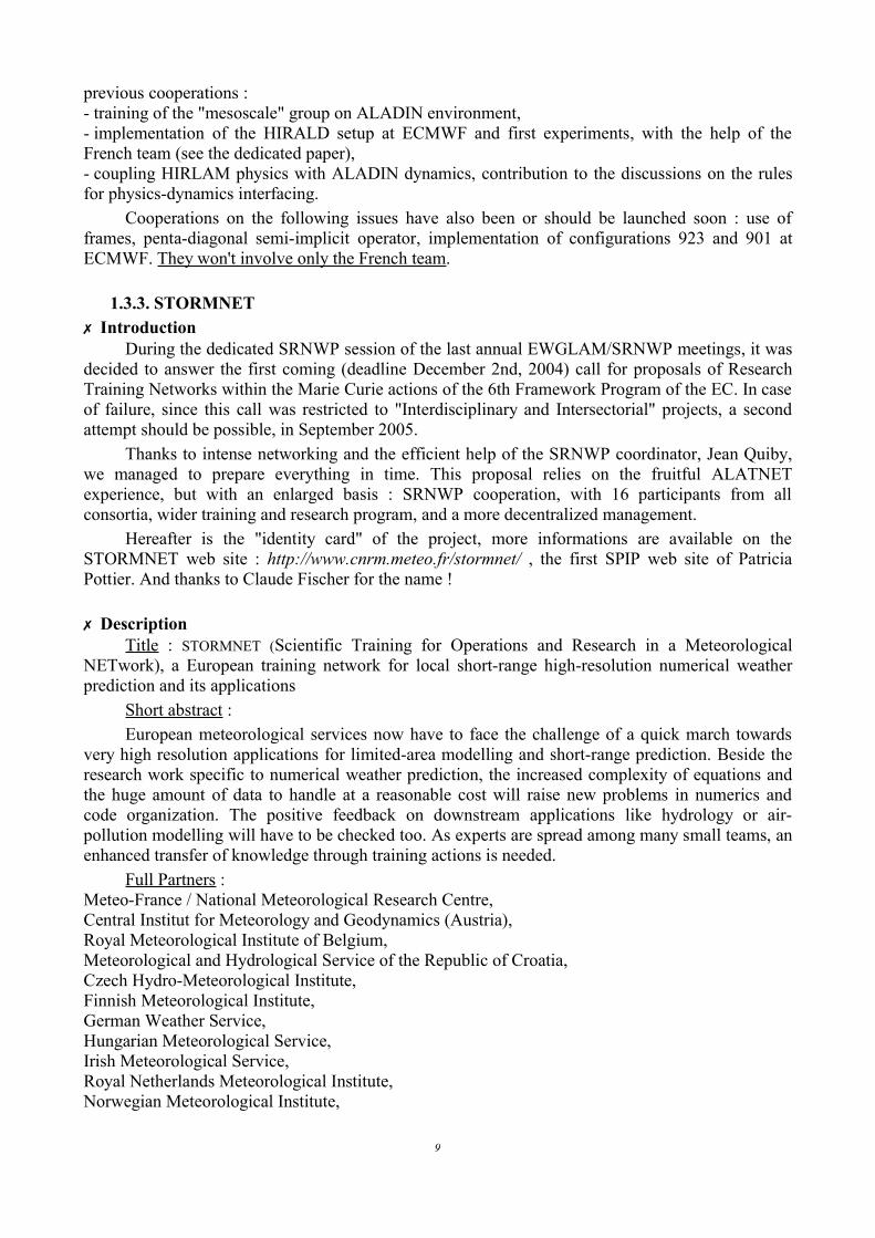
• New balance equations for Jb to take into account the ageostrophic motions• Variational quality control• New climatology for aerosols and ozone fields used by the radiation scheme• Tuning of a Rayleigh damping coefficient on temperature in the 2 uppermost levels• Reduction of 25 % of the thermal inertia for vegetation amplifying the temperature

diurnal cycleThese modifications have been tested against the operational ARPEGE version during 73 days

17

and the new version present improved results (see Figure 1) for practically all the meteorologicalparameters.

The subjective evaluation of both forecasts every day during more than 2 months has revealedthat the improvement of this new version is visible for a forecaster after 72 hours with about thedouble of better forecasts than worse forecast for all the cases where differences existed.

It is hoped that this new version will provide better initial conditions and lateral boundaryconditions for all the ALADIN LAM nested in ARPEGE. 2.2.2. Winter new version: modification of the mixing lengths of the turbulence scheme

A new formulation of the mixing length has been proposed by E. Bazile (Météo-France) andhas been tested against the GABL data set (the presentation is on the following web sitehttp://www.cnrm.meteo.fr/ama2004/) and is being tested during this winter. 2.2.3. Towards a new ARPEGE schedule: objective and intermediate steps

The current ARPEGE schedule, which drives the LBC provision for all partners includingFrance, has been constant since 1994 for the 00 and 12 UTC runs. At that time the ARPEGEassimilation scheme was Optimal Interpolation, with very limited capacities for ingesting satellitedata, and therefore very little impact of waiting for this data before starting the analysis.

The current schedule is not well adapted to the internal needs of Météo-France. As often inmeteorology, the most crucial issue is the availability in the early morning. The current scheme isnot so bad in wintertime, but since it is constant in UTC time while our users, and therefore ourwhole production, are based on local time, the summertime period is more problematic.

As presented in the 2003 Assembly of ALADIN Partners in Krakow, we have the "final"objective of having an ARPEGE suite that is constant in local time (or that we keep in UTC butchange by 1 hour twice a year to mimic a constancy in local time), covering at least:

- night run : Day D0 and D1 at 3h30- morning run : until D3 at 7h or 7h30- noon run : until D1 at 13h30- evening run : until the current D2 (the future D1) at 19h or 19h30.

The runs are intentionally not referred by a classical UTC stamp, the assimilation schemes allowingfor possibilities largely exceeding our current classical 6-hour windows.

For a series of reasons, the final objective cannot be met at one go. A first intermediate stepwas made last summer, with an additional preliminary ARPEGE run on 00 UTC with a 1 h cut-off,providing outputs shortly after 3h30 (by 3h45 actually); this run known as "PACOURT" endedwhen going back to wintertime end October 2004. For the summer 2005 the first goal is to have anoptimised PACOURT. Gérald Desroziers at GMAP tested various configurations, includingextended 4D-Var windows like [15 UTC - 01 UTC]. Finally, because the main issue related toPACOURT is the ability to capture or not a minimum of the 00 UTC radiosondes that arrive late insummer, the most promising candidate for 2005 is not such an extended 4D-Var, but a cheaper 3D-Var FGAT, allowing to wait a little longer for observations. The next steps will come later in thesummer, when we'll try to slightly delay the other runs in order to get closer to the final objective :the classical 00 UTC run becomes the morning run, the 06 UTC; then we'll have to consider thepossible merge of the current 12 and 18 UTC runs into a single one, leading to a scheme with 4daily runs again after a transitional period with 5 daily runs.It's difficult to give a precise timetable for all the steps, because the related potential problems havea huge variety and sometimes complexity. In fact part of our suite and of the tools that use it havebeen built, year after year, under the unconscious assumption that the ARPEGE schedule was frozenforever. So things are not as easy to move as it could look from outside. Anyway, the newPACOURT will be installed in March (the summertime period starting end of March), but the nextsteps are by any mean not expected before June. It is even likely that we won't be able to finalise thewhole process in 2005. Further news later this year.

18

For the ALADIN partners, in order to smooth the transition to the new ARPEGE schedule,several actions can be taken. First LBCs can be produced if requested on the current 06 and 18 UTCruns. Some partners already use this facility which makes available, at any moment, a reasonablyfresh set of LBCs (while using only the 00 and 12 UTC runs obviously leads to larger gaps). Then itcan be considered at some stage this summer to also produce LBCs on the PACOURT run.Eventually the local ALADIN data assimilation offers to each partner separately a way to adapt hisown NWP schedule to his own needs, the large-scale information provided by ARPEGE at least 4times a day keeping a good quality and the locally analysed fine scale bringing the last momentdetails.

19

Fig. 1: Comparison of the operational forecast and the new version against the TEMP observations. The isolines of thegeopotential are plotted every meter. The green isolines correspond to an improvement and red ones to a deterioration.

20

2.3. AUSTRIA (more details [email protected])

There have been no changes in the operational ALADIN system (CY25) at ZAMG since thelast Newsletter.

2.4. BELGIUM (more details [email protected])

For the operational aspects of ALADIN forecasts, these last months, we have encounteredmany problems with our SGI ORIGIN 3400 system. Under some specific circumstances, whenrunning ALADIN, a general crash of the machine occurs. This very tricky bug is located in thegeneral SGI-IRIX kernel and seems related to the "large page" option which allows to accelerateALADIN execution by about 15 %. Up to 12 kernel-cores have been made with a close SGIcollaboration, without successfully pinpoint the exact problem.

We also plan to switch to cycle 28T3 soon, in March 2005.

2.5. BULGARIA (more details [email protected])

No change along the last months, upgrade scheduled for spring 2005.

2.6. CROATIA (more details [email protected],[email protected])

2.6.1. IntroductionThere were no important changes in the Croatian operational ALADIN suite. Operational

version is still based on AL25T1_op2. More details in Newsletter 26.Model versions 28T1 and 28T3 were not ported on SGI.Prague physics package + SLHD was ported in Zagreb. Configuration 001 is ~75 % more

expensive in time consumption and ~50 % for memory consumption, what is significantly morethan on Prague SX6. At the moment we are not sure what is the reason for such a big difference intime and memory consumption.

Results for one of the performed tests for a "fog and stratus" case is shown below.

2.6.2. Test of new Czech setupFirst tests are very promising for the studied "fog and stratus" case.Example of verification plots for two points (one in inland, Zagreb-Pleso, and one on seaside,

Dubrovnik-Aerodrom) for the 14th of December, 2004, start at 00 UTC, are presented hereafter.

21

Fig.1 Comparison of old set-up (red), new Czech set-up (orange) and SYNOP data (violet points)

The amplitude of the error on 2-m temperature is significantly reduced for station Zagreb-Pleso and results for sea-side station are better too.

There is a problem in anticyclonic situations, the model has a tendency to reduce the highpressure. Even for this problem the new setup gives better results. Higher SIPR (semi-implicitreference pressure) further improves the result but does not cure it completely.

More case studies are under way. Reduction of time and memory consumption or upgrade ofthe computer is needed to put the new Czech setup in operational suite.

2.7. CZECH REPUBLIC (more details [email protected] )

2.7.1. Operations✗ The ALADIN/CE suite was switched to mean orography and modified physics on:

07/09/2004 at 12 UTC network time for the production run and at 06 UTC network time forthe assimilation cycle.

The corresponding parallel test has the identification name ADN. Here below is the fullmodset description (roughly in decreasing order of importance):I) Activation of the SLHD option for the horizontal diffusion processes. Most but not all of the

current linear spectral horizontal diffusion process is replaced by a modulation of the strength ofthe damping properties of the semi-Lagrangian scheme, via the choice of the interpolationoperators. The important fact is that this modulation is depending on the deformation field. This

22

helps avoiding false small-scale developments and better structuring rightly forecast ones. Thereis also a positive impact on the upper-air temperature scores.

II) Use of the new version of ACRANEB (quality equivalent for the atmospheric part to that ofFMR15, but without need to have an intermittent calling sequence) with all its novelties(LRMIX=.TRUE., LRPROX=.TRUE., LRSTAB=.TRUE., LRTDL=.TRUE. andLRTPP=.TRUE. with LRAUTOEV=.FALSE. and LREWS=.TRUE.).

III) Use of the random/maximum overlap for clouds instead of the random overlap(LRNUMX=.TRUE.). This change, together with the one above and the one below, brings asmall but systematically positive contribution to all kinds of scores.

IV) New "mixed" version of the Xu-Randall cloudiness scheme: one comes back to the publishedtuning of the X-R function (QXRAL=100.), the critical humidity (HUC) profile is computed inAPLPAR with a slightly different formula (3 coefficients rather than 2) and a tuning that matchesthe ZAMG proposal for quite lower values away from the PBL, QSSUSV is equal to 250 and acontinuous function with an intercept at 0.925 replaces the QXRHX=0.99 threshold, thisdifference compensating the effect of the HUC decrease. All these changes roughly keep thesame averaged structure of cloudiness (in mid-latitudes) but with a far less 0/1 behaviour and aslightly better vertical distribution.

V) Suppression of the envelope orography and introduction of the new drag/lift scheme with therecommended values (LNEWD=.TRUE., LGLT=.TRUE., GWDSE=0.02, GWDCD=5.4,GWDLT=1., GWDPROF=1., GWDVALI=0.5, GWDAMP, GWDBC and HOBST remaining unchanged).The pluses (better circulations and reduction of the precipitation dipole of errors, better scores at850 hPa) and minuses (too weak 10 m winds near mountains and too strong reduction of Foehneffects, hence worse scores at the surface) of this change roughly compensate each other.

VI) Activation of the "moist gustiness" option (LRGUST=.TRUE. with RRSCALE=1.15E-04,RRGAMMA=0.8 and UTILGUST=0.125).

VII) Computation, over sea, of a roughness length for heat and moisture that, while remaining closeto the one for momentum at small surface wind values, saturates far earlier for strong winds. Thelatter two points help getting a better simulation of the famous "Black-Sea" case.

VIII) REVGSL=15 to damp fibrillations around 0°C while keeping a still physically realistic valuefor this parameter (ratio of the fall speeds of rain and snow).

IX) Quasi-monotonous interpolation for specific humidity only.X) RCIN=1 in order to prevent one convective cloud low down to un-physically trigger another one

higher up across some rather deep stable and/or dry layer (and the same upside down inACCVIMPD).

XI) A different security tuning from the ARPEGE one for the "King-Kong-butterfly" syndrome:GCSMIN=5.5E-04.

XII) Mesospheric drag like in ARPEGE.

The above mentioned set of modifications is a synthesis of the work of many people inside theALADIN project. The decision on the operational switch was a trade off between better (PBL toptemperatures, precipitations) and worse scores (bias of screen-level temperature and wind). Betterresults prevailed, however, as well as the conscience that where the worsening of results occurred,we very likely have to do with a case of compensating errors. That is why we shall concentratewithin the forthcoming months on the screen level values of wind and temperature.

✗ The ALADIN/CE suite was switched to the new modification concerning the inversion-layerclouds on:

20/10/2004 at 12 UTC network time for the production run and at 06 UTC network time for

23

the assimilation cycle.The corresponding parallel test has the identification name ADP. This modification entered

the operational suite just at the beginning of the stratus season, so typical for Central Europe. It isbased on the previous work of Harald Seidl and Alexander Kann. It is however a bit algorithmicallyimproved: when a sufficiently thick inversion layer is detected, its temperature is cooled in someproportion of its vertical temperature gradient in order to re-compute the saturation profile used bythe cloudiness scheme.

For the time being, there are two tuning parameters. The first one, RPHIR, is a minimumthickness of the inversion layer for which the scheme is activated. It was tuned to 1750 J/kg (app.175 meters). The second one, RPHI0, is the length scale for the temperature vertical change toachieve the desired cooling. It was tuned to 1250 J/kg. Tuning was made for the November 2003period where we had a couple of situations with stratus, where the reference forecast missed low-level clouds (Figure 1) compared to observations (Figure 3). We could observe a weak improvementnot only regarding the amount of low-level clouds (Figure 2) but also in temperature scores. Sincethe scheme has a positive local feedback between cloud and inversion strength we verified that wedo not obtain an excessive amount of clouds.

However it should be stressed out that this is not a final solution to the low-level cloudssimulation problem. It is simply the first step in a good direction and already helpful in theoperational forecast.

At the same time a new diagnostic PBL height (development of Martina Tudor) was put inservice, after a set of off-line tests.

✗ The ALADIN/CE suite forecast length was increased up to 54h on:07/12/2004 at 12 UTC network time for the production run.

This was enabled by the availability of the ARPEGE coupling files for +51h and +54h from06/12/2004.

24

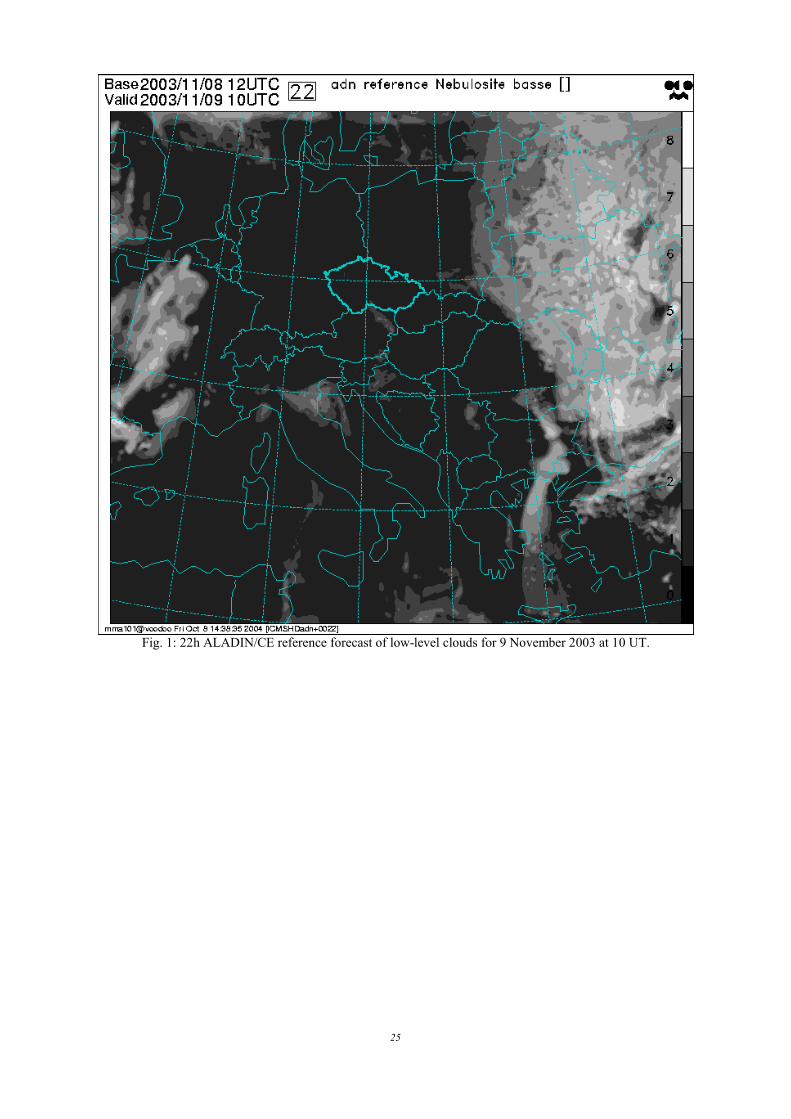
Fig. 1: 22h ALADIN/CE reference forecast of low-level clouds for 9 November 2003 at 10 UT.

25

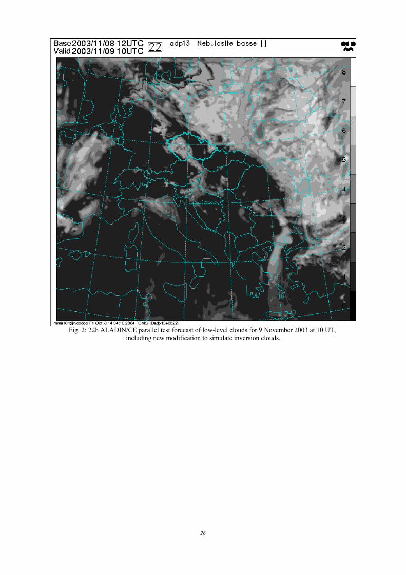
Fig. 2: 22h ALADIN/CE parallel test forecast of low-level clouds for 9 November 2003 at 10 UT, including new modification to simulate inversion clouds.

26

Fig. 3: NOAA picture from 9 November 2003 at 9:43 UT. Yellowish color shows presence of low cloudiness.

2.7.2. Parallel Suites & MaintenanceThe two main parallel suites, ADN and ADP, resulted in the successful operational

applications. There were other less successful suites, testing an alternative Ekman spiral simulation(ADO, ADQ and ADR). These suites were declared as void since there is no plan to continue withthis specific topic.

In the second half of 2004 we spent a lot of time on porting the cycle AL28T3. It was namelydue to the new data-flow structure used in the model as well as new style of using the interfaces atevery routine. On the other hand we managed to optimize rather well the code for the NEC-SX6platform. For example, despite more computations, forecast runs at about the same speed as it didwith the cycle AL25T1. Concerning lancelot (ee927) , it takes more memory (as found on VPP) butit runs almost three times faster compared to AL25T1.

We phased all the locally modified physics (content of ADN and ADP suites) to AL28T3 andwe are about ready to verify this cycle in a parallel suite. Here it should be mentioned that the ADNand ADP modifications are already phased into AL29T1.

There will be no further development and/or suite on the currently operational cycle AL25T1.On the other hand we still ought to validate research configurations with AL28T3 including theODB use.

27

2.8. FRANCE (more details [email protected])

Similar changes as in ARPEGE along the last months.

2.9. HUNGARY (more details [email protected])

In the second part of 2004 basically there were no changes in the operational ALADIN suite atthe Hungarian Meteorological Service.

The parallel suites were kept active and inter-compared objectively and subjectively :• ALADIN dynamical adaptation in 12 km resolution, • ALADIN 3D-VAR in 12 km resolution using surface (SYNOP), radiosonde (TEMP) and

satellite (ATOVS) measurements.Cycle 28 was installed and intensively tested for different model configurations. At the end of

the year the new cycle was also considered in the subjective evaluation, therefore beside theobjectives scores some subjective impression was also obtained.

Late summer our new IBM server was installed in the new computer room (on the groundfloor) of our Service, the main characteristics of the new machine are as follows :

• IBM p655 cluster server with 32 processors (clock rate: 1,7 Ghz), • Available memory : 4 Gbyte/processor, • Peak performance : cca. 8 Gflop/s per processor.

At the end of the year it was decided to modify the operational configuration of the modelwith the following main aspects :

• Horizontal resolution : 8 km, • Vertical resolution : 49 levels, • Grid : linear, • 3D-VAR data assimilation using surface, upper-air and satellite data.

The new model settings were intensively tested in the new machine and the implementation ofoperational procedures is on progress and should be completed at the first part of 2005.

2.10. MOROCCO (more details [email protected])

The present status of operational suites is described in the R&D report.

2.11. POLAND (more details [email protected])

Upgrades were not possible due to the limited computing ressources.

2.12. PORTUGAL (more details [email protected])

During the second half of 2004 few upgrades have taken place on our operational system.New observation stations have been introduced in the objective verification procedures. Besides, anew chart representation has been introduced under the Metview (ECMWF) batch environment forforecasting purposes.

28

2.13. ROMANIA (more details [email protected])

In agreement with our colleagues from Bulgaria, the SELAM domain for coupling files wasincreased from 90×64×37 to 120×90×41 points, keeping the same horizontal resolution.

For ALADIN–Romania, the domain size was kept and only the number of vertical levels wasincreased (from 31 to 41). The operational chain was completed by a new integration of theALADIN model, over the coupling domain, in order to provide the necessary atmospheric data forBlack Sea applications.

Old coupling domain New coupling domain

2.14. SLOVAKIA (more details [email protected])

2.14.1. SummaryIn the past, the LAM NWP data used at Slovak Hydro-meteorological Institute were received

from the ALADIN/LACE applications running at Météo-France in Toulouse and later at CHMI inPrague. After the end of common LACE operations, the kind offer of our colleagues from ZAMG,Vienna to use their ALADIN outputs covered our needs. Also, the local version ofALADIN/Slovakia was running at SHMI on the workstation over a rather small domain. However,in the course of time the ALADIN model products became the main source of information for ourforecasters and also serve as a basic input for numerous other applications. The need for our ownoperational ALADIN application over a European domain was obvious, both to fulfill increasingrequirements for new products and to have own control of the model timing and behaviour.

The purchase of the supercomputer at the beginning of 2004 allowed us to substantiallyupgrade the ALADIN operational suite at SHMI. The model is now running over the whole LACEdomain. All local applications were ported to the new computer under a unified operationalframework (run_app system). Almost all manpower of our NWP team was devoted to this taskduring the first half of 2004. Full operational status of ALADIN/SHMU started on July the 1st,2004.

The new HPC computer, ALADIN model version, domain and operational suite are describedbelow.

2.14.2. The new operational ALADIN setup✗ The new computer

The new computer at SHMI is an IBM @server p690 with code name Regatta. Its hardwareand software characteristics are described below and a picture is shown. More details can be foundon www.zamg.ac.at/workshop2004/presentations/olda.ppt.

29

HW : IBM @server pSeries 690 Type 7040 Model 681 32 CPUs POWER 4 Turbo+ 1.7 Ghz 32 GB RAM Memory IBM FAST T600 Storage Server EXP700, 1.5 TB

SW : AIX 5.2 Fortran compiler XLF 8.1.1.0 C,C++ compiler Engineering and Scientific Library ESSL Mathematics Library MASS 3.0 Parallel Environment (MPI): PE 3.2.0.16 LoadLeveler 3.2

Brief historical outlook : The Invitation To Tender was declared in June 2003, the evaluationsran during October 2003 and according to final decision of evaluation committee IBM @serverRegatta p690 was chosen. The contract was signed in December 2003 and the computer wasdelivered, tested and accepted in January 2004. The porting, optimization and validation ofALADIN source code together with other applications and tools could start. For this, some help wasobtained from The Products & Solutions Support Centre of IBM in Montpellier (porting ofALADIN code, optimisation of the code, optimization of memory manager and I/O, provision ofreliability of operational suite: AIX Work Load Manager & LoadLeveler & Vsrac).

✗ The ALADIN modelThe domain of ALADIN/SHMU covers the whole RC LACE area with an horizontal

resolution of 9 km, having 320×288 points in quadratic grid. There are 37 vertical levels. Moredetails are in the table below, the model domain is also displayed.

30

Illustration 1: ALADIN/SHMU model domain and orography

Domain size 2882×2594 km (320×288 points in quadratic grid)Domain corners [2.19 ; 33.99 SW] [39.06 ; 55.63 NE]

Horizontal resolution 9.0 kmVertical resolution 37 levels

Time step 400 sLBC data ARPEGE, 3 h frequency

Code version AL25T2

The model runs twice per day up to 48 hours in dynamical adaptation mode. Lateral boundarydata provided by ARPEGE are downloaded using internet, and backup is done by RETIM2000system (about 40 minutes slower than internet). Whole suite in optimal case needs about 60 minutesto finish. Hourly model outputs are available for further post-processing and visualization. Theyalso serve as the basic input for numerous applications like automatic point forecasts, dispersionmodels, hydrological models etc. Data for the PEPS project are provided as well.

The verification of ALADIN/SHMU outputs is done in two ways : locally only surfaceparameters are compared against observations over Slovakia, and data are also sent for processing inthe ALADIN verification project.

✗ The operational environmentThe operational suite is based on the in-house developed system of Perl scripts and programs,

and enables on-line monitoring and documentation (accessible via pocket communicator as well).More details can be found at web page www.zamg.ac.at/workshop2004/presentations/martinb.sxi.An example of the diagnostics for last 30 days is plotted on Figures 2-5. Given the importance ofthe ALADIN/SHMU products, the non-stop human monitoring of the operational suite startedrecently. One of the handy on-line monitoring diagnostic tool (number of processes of nwp001 user)is shown on Figure 6.

31

In case of unexpected failure of the operational ALADIN run, a mutual backup was agreedwith our colleagues at ZAMG. The remains of the system used in the past to produce data for SHMIat ZAMG are used now to generate the minimum dataset needed for SHMI. These data are dailydownloaded.

The privilege of the operational jobs on the machine is guaranteed by submitting all jobsthrough LoadLeveler batch queueing system, which together with Work Load Manager controls andallocates the system resources (CPU, MEM etc.). The operational suite is launched via a special Perlscript scheduled in the crontab. This script reads all operational configuration files and sets theapplication dependencies, number of used processors, memory requirements etc. All operationalapplications are then submitted as a single multi-step job into a dedicated LoadLeveler class (exceptthe applications monitoring the products transmission which are submitted into another class withlower priorities but within the same multi-step job). However, there is still some residual problemwith the preempting of non-operational jobs.

Active monitoring of the applications is done internally by the run_app system itself. It ispossible to switch on/off an ALERT for each application separately. In case of application failurethe automatic ALERT will be sent immediately to the mobile device and the person on duty will beinformed (or even woken up). Using the "pocket" version of the monitoring system he/she canbrowse the application logs, statuses and documentation then and if possible repair the suiteremotely.

2.14.3. Local R&D work and Future plansThough the implementation of the new ALADIN operational suite was a quite huge task, the

new computer was used for other R&D work. In NH dynamics, the technical cleaning of the codewas done and the theoretical study of the pathological behaviour related to horizontal diffusiontreatment (so-called chimneys) was performed. The dynamical adaptation of the wind field over theterritory of Slovakia with a 2.5 km resolution and hourly outputs, for the purpose of atmosphericdispersion modelling, was run. New diagnostics indexes to identify severe weather phenomena(Storm to Relative Environmental Helicity – SREH, Bulk Richardson Number – BRN) wereimplemented and validated. CY28T1 and T3 export versions were ported. Testing in parallel suite isplanned for the nearest future.

For the longer term plans, first of all the prolongation to 54 h (and possibly up to 72 h) isscheduled. Then the investigation of blending assimilation is planned together with porting,implementation and testing of ODB software during the first half of 2005. Also some LAM EPSactivities will start in cooperation with other RC LACE partners. Systematic improvement of theoperational ALADIN model version via ALADIN-2 and AROME projects is implicit.

32

Illustration 2 : LBC download (12 UTC), internet Illustration 3 : LBC download (12 UTC), RETIM2000

Illustration 4 : end of the suite (12 UTC) Illustration 5 : backup data(ZAMG) download (12UTC)

Illustration 6 : Monitoring of operational suite - "EKG"

33

2.15. SLOVENIA (more details [email protected] )

During the second half of 2004 few changes were introduced into the operational suite.Visualization of ARPEGE model on some standard pressure levels based on coupling files data wasincluded. Operational production of products for the PEPS project started in July. Meteorologicalservice from Albania asked for some ALADIN products, so from the end of the year some picturesare made available to them at our ftp server.

The coupling files from the ARPEGE model are transfered only via Internet from Toulouse. Inthe year 2004 the files were significantly delayed 7 times (1.9%) in the morning (after 4:30 UTC)and 17 times (4.6 %) in the afternoon (after 16:30 UTC). Main reason for delays was slow internettransfer rate; a few times the connection to sirius1 or sirius2 was not possible or files appeared latein the database. The number of cases of missed or delayed products has been decreased in year 2004(not taking into account the second half of December).

The upgrade of cluster system software was performed in mid-December 2004. Theoperational system on the computing and master nodes was upgraded from RedHat 7.3 to Fedoracore 1 and SCore software (the one which governs the distribution of computing jobs on the cluster)was upgraded from version 5.4 to 5.8. To have the upgrade as smooth as possible the wholeprocedure was carefully planed, a test cluster with the new version of software was built, but evenby executing the procedure unforeseen problems occurred and operational suite was seriouslydisturbed many times during the 3 week period. However, the problems were solved one by one andthe Tuba cluster is again in fully operational status. The main message of the upgrading procedure isthe importance of proper cluster file system which has been neglected so far. We are looking nowfor an alternative to NFS. From now on we expect improved stability of the cluster and even someperformance gains due to use of Intel Fortran compilers.

It is planed to upgrade the ALADIN cycle in operational suite as well (from 25T1 to 28T3).Code itself compiled fine but there are still some unresolved problems with xrd library manifestingin configuration ee927. Other configurations run fine. We are still working on the problem and weexpect that the new cycle should become operational during mid-February.

We performed different tests on some new architectures (i.e. Opteron64) with differentversions of compilers (PG, PathScale, Intel, Lahey) and we have to report that some of thecompilers are having problems with the new EGG routines. We are still investigating the problem.

2.16. TUNISIA (more details [email protected])

Significant changes in coupling: see the R&D report.

34

2.17. RSEARCH & DEVELOPMENTS AUSTRIA

2.17.1. INCA–A high-resolution analysis and nowcasting system based on ALADINforecasts

A common characteristic of today's numerical weather prediction (NWP) models is that theirforecast errors in the nowcasting range, up to a few hours, are not significantly smaller than those at+12 or +24 hours. This is because NWP models start from analysis fields that may already differsignificantly from observed values at the observation locations. No matter which method is used, beit variational analysis, optimum interpolation, or nudging, NWP analyses are strongly constrainedby the model's dynamics and physics. The INCA analysis module is specifically designed forforecasting applications, not for model initialization. For temperature, humidity, and wind it isthree-dimensional and has a time resolution of 1 hour. For precipitation it is two-dimensional, witha time resolution of 15 minutes. Horizontal resolution is 1 km, vertical resolution 200 m. Thevertical coordinate is geometric height z above a "valley floor surface" which is basically the lowerenvelope of the terrain.

The analysis starts with an ALADIN forecast as first guess. Then an error field is created fromthe differences between the model forecast and the actual observations at the stations. Since wehave a certain number of mountain stations, we can compute the error field in three-dimensions. Inthe future we may include AMDAR data into the system to obtain improved vertical structures. Thespatial interpolation of the point differences is done by distance weighting in the horizontal, andpotential-temperature distance weighting in the vertical. The variables used are potentialtemperature and specific humidity up to now but will be changed to liquid water potentialtemperature and total water content in the future (e.g. to get a better analysis of low clouds).Figure 1 shows as an example analyses of 2 m temperature and relative humidity. It is a low-stratussituation and in the relative humidity analysis one can see the boundary of the cloudiness at theAlpine foothills. A rather complex temperature structure arises because of the presence of thestratus in low areas, leading to inversions, and the normal decrease of temperature with height in theAlpine areas.

Nowcasting of temperature and humidity is currently based on a simple weighting algorithmthat gives a smooth transition from the analysis to the ALADIN forecast after several hours.Figure 2 shows the reduction in temperature forecast error that can be gained. In the future, errormotion vectors (EMVs) will be used instead of the prescribed weighting. This will allow bettercompensation of phase-shift errors in the ALADIN forecast, for example those associated withfronts.

More information : [email protected]

35

Fig. 1: INCA 1 km Analysis of 2m temperature and 2m relative humidity during a low-stratus episode. It is based on theoperational ALADIN forecast, station observations, and high-resolution topographic data.

T2m forecast 28 Jan - 09 Feb 2005, all stations

0

0,5

1

1,5

2

2,5

0 1 2 3 4 5 6 7 8 9 10 11 12

Le ad time (h)

Me

an a

bso

lute

err

or (

K)

A L A D IN

IN C A

Fig. 2: Comparison of ALADIN and INCA T2m forecast error (mean over ~140 stations) as a function of lead time.

36

2.17.2. Quantitative evaluation of the orographic precipitation problem in ALADINDuring orographic upslope flow situations, the ALADIN model tends to predict excessive

rainfall on peaks and ridges and rather dry conditions with negligible precipitation in valleys andbasins. Moreover, the modelled precipitation field is connected to the flow-oriented steepness of themodel topography in an extremely close and direct way (Figure 3), most likely much closer than inreality.

Fig. 3: Typical example of a 24-hourly ALADIN cumulative precipitation forecast (colors). The model topography isshown in isolines, the actual terrain by shading.

We think that the overestimation of upwind/downwind and peak/valley precipitation contrastsis to a large degree caused by the diagnostic treatment of cloud water in ALADIN. It causesprecipitation maxima to more or less coincide with vertical velocity maxima in the model, whereasin reality considerable amounts of cloud water (and also precipitation, in the case of snow) may beadvected onto the downwind side of a mountain.

In order to obtain a quantitative diagnosis of the problem, ALADIN point forecasts of 24-hourly rainfall (for the lead time period +0 to +24h) are compared to station observations. Thecomparison is performed on monthly precipitation sums. Figure 4 shows results for the months Dec2004 and Jan 2005, where a number of orographic upslope events affected the northern Alpineslopes. Figure 4 shows that inner Alpine valleys generally show ratios < 1, and < 0.5 in severalareas. Along the northern Alpine rim a systematic overestimation of precipitation by a factor of 1.5-2 is found.

It is instructive to analyse some of the small-scale features, such as the precipitation ratiomaximum near the center of the domain, South-East of the city of Salzburg. This is an area that is inreality located on the downwind side of a steep, high mountain (Dachstein) and experiences strongsheltering effects. The model, however, does not resolve the valley. Instead there is an area with arelative topography maximum. Thus (as can be seen in Figure 3) orographic precipitationenhancement is predicted instead of sheltering.


37

Fig. 4: Interpolated ratio of precipitation predicted by ALADIN (+0 to +24 h) and observed at stations during themonths Dec 2004 and Jan 2005. Inner Alpine valleys generally show ratios <1, with values <0.5 in many places. Alongthe northern Alpine rim a systematic overestimation of precipitation is found.

2.17.3. Stratus predictionUsing the Seidl-Kann (SK) inversion cloudiness scheme, satisfactory low stratus forecasts are

obtained for lowland areas in the operational ALADIN run at ZAMG. A good stratus prediction inbasins (even if they are very wide, such as the Linz basin in Upper Austria) was however found torequire switching off, or setting to a very small value, the "horizontal" diffusion of temperature.This is because the spurious vertical component of this diffusion too strongly smoothes inversions.Thus, in order to get the full benefit of the SK scheme operationally, the T-diffusion would have tobe switched off. Since we were not sure whether this has detrimental effects in situations withstrong temperature gradients, a few tests were carried out, for example on the storm case of 19 Nov2004. The results showed no obvious problems, and little difference in forecast fields between theexperimental and operational runs. This means we will most likely switch to a rather small T-diffusion operationally.

More information : [email protected] 2.17.4. Evaluation of mesoscale precipitation forecasts in the Southern Alpine area

A comparison of precipitation forecasts for different regions in Austria shows that thenorthern upslope precipitation areas (Salzburg, Upper Austria) show a higher predictability than theupslope areas in the South (Carinthia). The orographic situation appears to be the main reason forthis. In the south, the primary upslope precipitation belts are the mountain ranges in Italy andSlovenia. Austrian areas are located downwind of these "primary" upslope areas. Several fall andwintertime heavy precipitation events (1999-2003) during southerly flows were analysed andcompared with ALADIN forecasts. The existence of systematic forecast errors for parts of Carinthiaand East Tyrol was documented and analysed with regard to the dependency on certain weathersituations. The results show that regions downwind of strong primary upslope areas show a highpercentage of cases in which the precipitation amounts are underestimated by ALADIN. Even in thepresence of synoptic-scale lifting (e.g. frontal passage), over-pronounced lee-side downward motionand overestimated loss of water in the upslope areas result in an underestimation of precipitationamounts in the downwind regions. Further it was examined whether comparison of upstreamsoundings (e.g. Udine) with ALADIN pseudo-TEMPs can give additional prognostic informationregarding precipitation patterns and the expected quality of the ALADIN forecast. The results showthat only in a few cases differences between TEMP and pseudo-TEMP can be linked withdeviations between observed and modelled precipitation patterns in the downwind areas.


38

2.17.5. Verification of dynamically downscaled windFor the 4-month period March-June 2004, 6-hourly forecasts (up to +48h) of

a) the operational (9.6 km) run, b) the dynad (2.3 km) run, c) the dynad (2.3 km) run without envelope, were compared. The main results are the following. There is little difference between b) and c), asexpected. The envelope is not important at this resolution. All stations taken together, there is noclear signal of improvement from a) to b). If stations are grouped according to elevation, a moderatepositive signal is found for the highest stations (2000-3400m), especially mountain top stations.Individual stations show up to 15-20% improvement in mean absolute error (MAE) in b) comparedto a), but there are also stations which show worsening of the same amount (that's why in the meanover all stations there is no positive signal). In most cases, the changes in MAE reflect to a largedegree simply changes in bias.

We had expected that at least for those stations which are inside deep valleys, and thus verypoorly represented at the operational resolution, the 2.3 km dynad run would bring significantimprovements both in wind speed and wind direction. It turns out this is not the case. Apparentlythe wind regime in those valleys is strongly influenced by thermally induced flows (valley winds)which are not improved by the dynad run.


2.17.6. Development of a LAM ensemble prediction system using ALADINLimited-area models provide highly structured forecast fields both in space and time.

However, often the small-scale features are extremely sensitive to uncertainties of the model and/orinitial conditions. To obtain a guidance for the forecaster with regard to this uncertainty, the project"ALADIN Limited Area Ensemble Forecasting" has been started at ZAMG. It is an ensembleforecast system with 11 members, in which perturbed initial conditions are created using a breedingmethod. In a second step, the Ensemble Transform Kalman Filter (ETKF) technique will be appliedto the breeding vectors. The NWP model used is ALADIN with reduced horizontal and verticalresolutions (16 km, 31 levels). The domain covers the whole of Europe and large parts of the NorthAltantic ocean.


2.18. BELGIUM

2.18.1. Stability and accuracy of the physics-dynamics interface(Piet Termonia)

The aim of this is the generalization of the work in a paper by Staniforth et al. (2002). Asshown during my lectures in the TCWGPDI in Prague, extending this to include algorithmic issuesimposed by the time-step organization rapidly leads to algebraic complications that are too tediousto be treated analytically. I proposed a way out of this by determining the stability of the scheme bymeans of a numerical maximization of the amplification factor. In the near future this method willbe applied to perform a comparative study between the time-step organization of ARPEGE/ALADIN (physics before dynamics, parallel physics) vs the ECMWF model (physics afterdynamics, sequential physics).

2.18.2. Monitoring the coupling-update frequency(Piet Termonia)

1. I have implemented the findings of my paper Mon. Wea. Rev., 132, 2130-2141, in cycle

39

28T2. This allows to operationally compute a warning index for information loss of the couplingdata due to a too long coupling update interval.

2. I have started writing a paper presenting a method to objectively determine the coupling-update interval, with the aim to tune coupling strategies in case of detected information loss.

2.18.3. 2 m temperature forecasts(Piet Termonia)

I also carried out some research on a proposed model output statistics to improve some bad2 m temperature forecasts of the Belgian operational ALADIN runs during winter. Since the largesterrors occur during stable conditions, I propose a correction of the 2 m temperature based on a timeintegration of the tendency computed by using the exchange coefficient for the temperature. Theresult can be physically interpreted as a temperature difference and is thus well suited to becompared with temperature errors. A quasi-linear relation can be identified between them. Testsduring last winter showed that, by exhibiting this linearity, the RMSE for the 24 h forecast range2 m midnight temperatures for ALADIN-Belgium could be reduced by about 1.3 degrees.

2.18.4. "Wavelet Jb"(Alex Deckmyn)

Research was continued on the use of complex wavelets for the representation of backgrounderror covariances. Such wavelets not only represent location and scale of features, but also have adirectional component (even though it is limited to a resolution of about 15°). The wavelets nolonger form an orthogonal basis like Fourier components, but instead a so-called "tight frame". Thisnon-orthogonal redundant transform increases the number of parameters but improves considerablythe representation of anisotropies and reduces the occurrence of artefacts in the local variance.

Work has been initiated on an experimental 3D-Var implementation using wavelets in thecontrol variable.

2.18.5. Adaptations to ALADIN of the Lopez micro-physical package (Luc Gérard)

See the dedicated paper.

2.18.6. Gravity wave drag(Bart Catry)

In 2004 I continued the work on the validation/tuning of the new mountain-wave-dragparameterization scheme in ARPEGE/ALADIN. This validation took place on three predictionscales: (1) semi-academical tests performed by ALADIN on an idealised flow over a complexorography (ALPIA) enables one to calculate momentum budgets which prove to be a gooddiagnostic tool; (2) regional scale tests using the Czech ALADIN-version produce verificationscores over Central Europe; (3) global tests using NWP ARPEGE render statistically significantscores over the different continents. Using these three scales one is able to cross-check the validityof the new parameterization scheme or parts of it.

We finally found values for the two new tuning constants ( =1.0 and =0.5 ). Thealready available constants were retuned using the above-mentioned method to find =0.020 ,Lt =1.0 and C d =5.4 . The new scheme was found to be resolution independent and usable

down to horizontal mesh-sizes of 5 km. Below 5 km the scheme appears to have an incoherentbehaviour suggesting that no mountain-wave-drag parameterization should be used at such scales.We were also able to show the clear improvement of the new lift scheme where the additional

40

rotation is now in the correct direction. All these improvements give one the opportunity to removethe envelope orography and use (even operationally) a mean orography, which has been tested forthe operational versions of ALADIN-CE and NWP ARPEGE.

At the end of 2004 I also started research on a multi-directional version of the current gravity-wave-drag scheme where the main goal is to have a better representation of the transport ofmomentum with height. This research should be finished by the end of 2005.

2.18.7. Physics-Dynamics Interface(Bart Catry)

Due to the decision that one should go from ALADIN to AROME through ALARO, with apossible cooperation of HIRLAM, the need of a new physics-dynamics interface became anecessity. Not only should this new interface be able to be implemented in these different models, itshould also be as flexible as possible to allow further developments concerning physicalparameterizations in the near future without having to make big changes to the interface.

My work on these issues has been limited for 2004 to the analysis part, i.e. the full declinationof the un-parameterized discretized equations with respect to the following problems : (1) accounttaken of the multi-phasic and baroclinic choices; (2) enthalpy conservation; (3) choice betweenm=0 and m=1; (4) optional projection of the heat source on temperature and pressure in thecompressible case. These so-called "governing equations" should be obeyed by all low-levelroutines (i.e. all parameterizations routines).

In order to close the above-mentioned set of equations, some routines will need to add so-called "diagnostic-equivalent" variables to their local input/output stream. We could conclude thatthis means that one should find an expression for the following pseudo-fluxes : condensation,freezing, evaporation, sublimation and two fluxes related to the auto-conversion for the liquid andsolid phases.

2.19. BULGARIA

2.19.1. New Integration Domain for ALADIN-BGA new integration for domain ALADIN-BG was created and tested. Its characteristics are as

follows :• - coordinates of the centre : 25.5°E, 42.75°N• - south-west corner : 19.27°E, 38.95°N• - north-east corner : 32.51°E, 46.22°N• - number of points : 108×80 (91×69)• - grid type : linear grid• - horizontal resolution : 12 km, NSMAX = 39, NMSMAX = 53

The corresponding set of climatological files was created. Increasing the domain size andtruncation led to an increase of the integration time by 45 % on average, and the 48 hours forecast iscalculated for 28 minutes, using both processors of the PC.

Post-processing for visualisation purposes is done on a latitude-longitude grid of resolution0.1° × 0.1°, using climatological files.

From the beginning of December 2004, a pre-operational suite based on this domain isrunning in parallel to the old one. The verification scores over Bulgaria are better than with theoperational suite.

41

It is planned to switch new suite to operations at the end of March. 2.19.2. Porting cycle 28T3

Technical stuff, not described here. 2.19.3. A lot of work in Toulouse !

2.20. CROATIA

See the report on operations.

2.21. CZECH REPUBLIC

2.21.1. ALADIN/MFSTEP configurationAs a result of the recent efforts the differences between ALADIN/CE and ALADIN/MFSTEP

were diminished to the necessary minimum. These differences in ALADIN/MFSTEP are: an extracomputation of the clear sky solar radiation flux; no use of the LRMIX option in ACRANEB due tocost reasons; absence of the last modification concerning the low-level inversion clouds (ADP).

Besides, there is also a change in the algorithm of the cycling. Due to the fact that theresolution of ARPEGE coupling files is relatively low, i.e. that there is a more important jump inresolution between ARPEGE and ALADIN/MFSTEP than usual, we had to introduce a lightincremental digital filter into the blending cycle. Otherwise we got higher root-mean-square error ofthe mass field despite a better bias – a clear sign of noise.

The ALADIN/MFSTEP application runs in its Target Observation Period (TOP) sinceSeptember 1st, 2004. This period is 6 months long. It will provide back a lot of interesting materialof validation, namely concerning the screen-level fluxes. 2.21.2. Bottom boundary condition

A correct application of the kinematic rule for vertical velocity at the bottom boundary (ws)was tested for the linear horizontal diffusion equation. The problem is that such a correct treatmentrequires computing the scalar product of the model lowest level horizontal wind with orographywithin the part of spectral space computations. The scalar product needs to be computed twice:using the horizontal wind prior and after the horizontal diffusion operator in order to compute acorrect tendency of ws for this equation. This is technically complicated and that is why weattempted to test various simplifying approximations. These tests however confirmed that there isno good approximation of the above-mentioned scalar products; otherwise a so-called "chimney"pattern occurs (but only at very high horizontal resolutions, of hundreds of meters, in presence ofquite strong horizontal diffusion).

We started to explore a possibility to compute this product using bi-Fourier coefficients; itwould anyway cost some communications. Thus the algorithmic strategy for 3D model has to bethought over. A comprehensive report on this work was written by Jan Mašek.

The problem may be solved to a large extent in case of the semi-Lagrangian advection, wherethe linear horizontal diffusion is substantially replaced by SLHD. 2.21.3. Tests of SLHD and gravity wave drag in the ALPIA framework

The plan was to explore more in depth the behaviour of SLHD in presence of mountainforcing in combination with the gravity wave drag parameterization. Therefore the ideal tool forsuch a study is an ALPIA-10km experiment. The topic was taken by a newcomer and for themoment it was rather a learning exercise. 2.21.4. SLHD developments

New SLHD developments (extension to ARPEGE, introduction of spline interpolators) and

42

maintenance were provided by Filip Váňa. Please refer to the relevant article in this Newsletter formore details.

2.22. FRANCE

2.22.1. IntroductionResearch around ALADIN restarted in La Réunion (in the Indian Ocean), the corresponding

work is described in a separate report.Not described hereafter are all the tasks related to project management and support to Partners

(not at all a minor contribution). They are partly mentioned in the Editorial part. 2.22.2. Source code maintenance✗ Introduction

As along the first 6 months of 2004 there was no rest for the phasing teams, from the deliveryof cycle 28T1 early July to the latest contributions to cycle 29T1 at the end of the year. However thetask was somehow alleviated since :

1. Many ALADIN phasers came to help. Thanks to Andrey Bogatchev, Nihed Bouzouita,Alex Deckmyn, Stjepan Ivatek-Sahdan, Cornel Soci, Oldrich Spaniel, Piet Termonia, AlenaTrojakova, Filip Váňa, and to the distance support !

2. A rotating supervision of phasing started. Claude Fischer was efficiently replaced by RyadEl Khatib for cycle 28T3, and by Ryad El Khatib and Yann Seity for cycles 29 and 29T1. The nextteam will involve Gwenaelle Hello and Patrick Moll (29T2 and 30).

✗ Cycles 28T1 and 28T2- July 2004

Cycle 28T1 is described in the previous Newsletter.A new cycle, 28T2, was created just afterwards. No export version was delivered, since it was

built as a reference for the summer parallel suite in Météo-France (see the report on operations).

- Contributions to 28T2 • From Christophe PAYAN (uti)

- Management of QuickSCAT observations• From François Bouyssel, Eric Bazile, Yves Bouteloup, Jean-François Geleyn (arp, sat)

- Changes in the ARPEGE radiation scheme (FMR15) : new 2d monthly fields for ozone andaerosols

- Vertical diffusion : changes in Louis' functions for the stable case, and in the computation ofinteractive mixing lengths

- Writing the short-wave downwards flux at surface in historical files- Model-to-satellite tool based on RTTOVS : cautions ! (new namelist NAMMTS not yet

working)- Changes in the ALADIN radiation scheme (ACRANEB_new)

• From GCO (uti)- Latest modifications for the extraction of observations

• From Jean-Marc Audoin (uti)- New fields (chemistry model) and new domains in PROGRID; new name for brightness

temperature.• From Patrick Moll (arp)

- One database per observation type, use of BUFR data for AIRS

43

- Variational quality control- Assimilation of AMSU-B, EARS, AIRS, QuikSCAT data

✗ Cycle 28T3- August 2004

This step aimed at providing a cleaner, more portable, code for the update of operationalsuites, taking into account the problems encountered in the porting of cycle 28T1 and someintermediate developments.

- A new export version was created in September, including the following : • Use of AIRS and AMSU-B (thinning, blacklisting, std dev.)

Thomas AULIGNÉ, Patrick MOLL, Florence RABIER, Delphine LACROIX• Bugfix on restart scheme

Ryad El Khatib• Bugfix on interactive mixing lengths (not yet active)

Eric Bazile• Bugfix for configurations with NFLEVG=1

Françoise Taillefer• Various bugfixes, mostly related to portability

Ryad El Khatib and ALADIN teams• Bugfix for the use of the linear grid in ALADIN (initialization of RNLGINC)

Ryad El Khatib under the control of Jean-François Geleyn • "model to satellite" code temporarily put off

Ryad El Khatib• Developments on the new ALADIN radiation scheme

Jean-François Geleyn via François BOUYSSEL• Bugfix on the adding of physical tendencies in the Eulerian scheme

Jozef Vivoda• Bugfix for coupling in case of d4 variable (NH)

Gwenaëlle Hello• Bugfix to use the "10 meters" wind SHIP data at the proper height in CANARI (when screening

is not called before)Françoise Taillefer

More explanations are available in the mails sent by D. Giard on September 10th, andM. Derkova on December 1st.

✗ Cycle 29- September-October 2004

This was a common cycle with IFS, with no scheduled export version. Hereafter is a shortdescription of contributions, from the ARPEGE memorandum prepared by GCO and the Minutes ofthe ARPEGE-IFS coordination meeting help on November 10th. For more detailed descriptions, seethe mail sent by D. Giard on February 15th.

Note that there is still a problem in RTTOV8, introduced by ECMWF. However, since theydidn't manage to solve it, the position is now : "we'll do with".

- ECMWF contributions to cycle 29 (starting from cycle 28) • CY28R1

44

- Humidity control variables generalised to arbitrary numbers of levels- Start of ODB port to Linux- METAR data monitored (new subtype under type 1) / ERS2 Scatterometer CMOD5 (update

of CMOD4) / Passive monitoring of MSG clear-sky radiances / AMVs - use of GOES- Diagnostic tool for influence of observations (LANOBS=.TRUE.)- Modification to trajectory for first time-step, Noise reduction for vertical trajectory in the

stratosphere (LSVTSM)- Higher top for 91 levels

• CY28R2- Modifications to get Linux version working (for benchmarks) / More GSTATS- Wavelet Jb coding (IFS wavelets) / New tests for 4D-Var components (LTESTVAR: Global

switch for tests, LCVTEST: Change of variable test, LADTEST: Adjoint test, LTLTEST: Tangentlinear test, LGRTEST: Gradient test, old LTEST)

- Clean-up of LARCHE• CY28R3

- 1D-Var rain assimilation / Cloud detection of AIRS / RTTOV-8 introduced / New variables inblacklist (rejection of SYNOP/METAR depending on local conditions)- Variational bias correction (tests started – interactions with the triggering of spurious verticalmodes in the stratosphere in the trajectory computation have been noticed)- Improvements in model error term in 4D-Var / Optional new control variable for O3- TL and AD of spectral RT (used in combination with grid-point Q)- Singular vectors to be orthogonal to a set of vectors- Random number generation with multiple independent seeds for EPS- More flexible handling of trajectory (grid-point and spectral fields) / SL buffer optimisationwith respect to GFL attributes- Bugfix for GRIB header

• CY28R4- Changes to scripts- Modifications to OBSTAT for satellites

- ARPEGE/ALADIN changes from 28T3 to 29 • Merge with the IFS developments• Cleaning of NH dynamics (removing now useless options)• Update / cleaning of CPGTL and CPGAD (split as for CPG some time ago)• Cleaning of physics interface (APLPAR etc.)• Merge of CNT4 : no more duplicated routines in the model libraries !• Diagnostics on physical tendencies (from Tomislav Kovacic et al.)• Warning indices in configuration 001 (from Piet Termonia)• SLHD developments (from Filip VANA)• Use of GRIBEX in FA files (from Denis PARADIS, see the dedicated paper)• Introduction of "radar" tables in odb• Full-Pos optimization (starting)• etc ...

45

✗ Cycle 29T1This is mainly a "cleaning" cycle, with some developments on top. Or rather this will be, since

there are still validation problems (mid-February).The main advances are the following :

• Cleanings and bugfixes• Merge with the ARPEGE parallel suite : interactive mixing lengths, use of AMSU-A AQUA... • Xu-Randall cloudiness and other developments in physics (from Radmila Brozkova)• New setup for horizontal diffusions (from Filip Vana, report available on the ALADIN web site)• New SL interpolations (from Filip Váňa, see the dedicated paper)• Some more for radar and SEVRI observations• Further improvements for portability (especially Linux)• Update of 923 (yes !), but only for parts 2-10 unfortunately

✗ Towards an improved portability

A huge cleaning of keys in the xrd library (and elsewhere) started last autumn (see e.g. thestay report of Nihed Bouzouita), and the test of the new cycles on various platforms (VPP, IBM, PCLinux) in now part of Toulouse validations. But there is still a lot of work.

A further step, as proposed by Jean-Daniel Gril, will be : - first, to take the FA/LFI package (or more generally I/Os packages) out of the auxiliary library,- second, to convert the FA/LFI code to F90, since it is now a rather peculiar mixture of F77 andF90, uneatable for some (many ?) compilers. Both "automatic" and "manual" changes will berequired. Help will be welcome !

Jean-Daniel Gril also updated PALADIN (mainly phasing up to most recent cycles) and othertools. Please don't forget to send him informations on any problem you met or any improvement youbrought, so that everyone may benefit from it.

✗ 2005 program- Cycle 29T2

Starting in March, with the help of Jozef Vivoda and Adam Dziedzic !Here is a provisional list of contributions collected by Claude Fischer :

• phasing of the AROME prototype (Yann Seity)• NH developments :

• "3TL Eulerian PC" (Jozef Vivoda)• advection of vertical velocity ("LGWADV", for d3 and d4 options) (Jozef Vivoda)• reorganization (Karim Yessad)• cleaner call to physics in Predictor-Corrector scheme (Martina Tudor, Gwenaëlle Hello)

• some more refinements for semi-Lagrangian horizontal diffusion (SLHD, Filip Váňa)• changes for ARPEGE physics (François Bouyssel, Yves Bouteloup) :

• simple micro-physics (Lopez scheme)• changes in radiation (RTTM)

• new rotated tilted Mercator geometry (Jean-Daniel Gril)• "Jk" cost-function in ALADIN 3D-Var (Bernard Chapnik, Claude Fischer)• (Ts - TL) in control variable (Ludovic Auger, see the paper on Var-Pack)

46

• corrections for the monitoring of radar observations (Eric Wattrelot)• + ...

More changes may be included, provided they are carefully validated and sent before mid-March.

- Cycle 30 There should be only one common cycle with IFS in 2005, with phasing starting in May.The main IFS contributions put forward in November were the following (cf mail DG 15/02) :

• new observations (AQUA, TERRA MODIS winds, NOAA-18, MSG winds, SSMI/S and AMSR,rain-affected microwave radiances, ground-based GPS water vapour, METAR data, ...)

• improved pre-processing of observations (variational radiance bias correction, Huber-norm forVarQC, ...)

• 4D-Var : better interpolation of trajectory and increments, grid-point q and O3 in inner loops, newM1QN3, cleaning of SL AD/TL, removing Jb from STEPO, pruning LOBSTL=.FALSE. ?

• some more changes in the data flow• new PBL scheme, ...

The reorganization of NH dynamics shall be continued. To propose other ALADINcontributions, do contact Claude Fischer !

- Cycle 30T1 ? One more cycle may be expected by the end of 2005, to take into account developments

related to :• the externalization of the surface scheme (the proposed roadmap is now available at :

http://www.cnrm.meteo.fr/aladin/scientific/reunions_surfex_190105d.pdf), • the physics-dynamics interface (APLXX calling all physical packages : Meso-NH - APLAROME

with a careful handling of missing fluxes –, ARPEGE/ALARO – with a management of missingvariables and the reduction of the m=1 option to a few dynamical and interfacing terms -,HIRLAM ... for more details please contact [email protected]),

• the improvement of portability, • etc ...

2.22.3. Dynamics, geometry and coupling✗ Design of ALADIN domains

- Rotated tilted Mercator geometry This new projection allows to focus on any part of the world, cumulating the abilities of the 3

previous types.Besides, but most important, it should allow to better account for distorsions of the mapping

factor (here a simple function of Cartesian coordinates m =cosh y /a ) in the semi-implicitformulation (using penta-diagonal operators as in ARPEGE), hence to run ALADIN-NH dynamicson very large domains.

A detailed documentation was written by Pierre Bénard and should be soon available on theweb site. The code should be available soon, too. The new definition has already been coded andvalidated in PALADIN and in the model by Jean-Daniel Gril. The Full-Pos implementation is onthe way and should be ready for cycle 29T2 (i.e. March).

47

- Clim files Configuration 923 was partly updated, taking into account the new definition of domains, the

new configurations, and some bug corrections introduced by Ryad El Khatib between AL15 andAL29 (Dominique Giard, Stjepan Ivatek-Sahdan). Parts 2-10 can now be run with cycle 29T1. Thenew options are : 8 : constants for ozone description 9 : aerosols10 : aqua-planet (all fields in 1 run)

Besides work started around scripts, for Olive (Véronique Mathiot) and for multi-domainupdates (Françoise Taillefer).

All the "clim" files used operationally in Toulouse, including those for coupling domains,were updated by Eric Bazile : they now include ozone-related and aerosol fields, and the additionalsurface albedos required for the new snow scheme.

✗ Vertical discretization- Definition of the vertical grid

A flexible procedure to define sensible hybrid levels (i.e. to compute the required A and Barrays) was written and documented by Pierre Bénard, considering the finite-difference approach.Everything is available at : http://www.cnrm.meteo.fr/gmapdoc/modeles/procedures/AandB.html . Itmust be underlined that additional constraints appear when using a vertical discretization based onfinite elements.

Besides, an increase of vertical resolution was evaluated in ARPEGE, adding 5 new levels inthe stratosphere to improve the assimilation of satellite observations.

- Study of the Vertical Finite Elements (VFE) discretization in view of non-hydrostatic (NH) modelling

The IFS model currently uses a VFE discretization based on cubic spline functions withcompact support (Untch et Hortal, QJRMS, 2004). In view of possible future NH modelling,ECMWF has recently asked the ALADIN group whether the current NH dynamical core ofALADIN could be extended for global modelling with their current VFE discretization.

48

This requires two main tasks : (i) extending the current LAM NH dynamical core to the globalcontext, which appears as a relatively technical task, mainly involving some modifications in thedesign of the semi-implicit scheme; (ii) extending the current finite-differences NH discretization tothe VFE context. This task appears as more scientifically challenging. A preliminary study showedthat a direct application of the current VFE discretization to the NH dynamical core was notappropriate (Bénard, 2004, http://www.cnrm.meteo.fr/gmapdoc/modeles/Dynamique/vfememo1.pdf).

The reason is that the current VFE discretization does not fulfils some mathematicalconstraints required for the vertical operators used in the semi-implicit part of the NH system (theseconstraints were not required for the primitive equation system). As a consequence, the current VFEscheme applied directly in the current NH kernel would result in an unstable model.

Several simple alternative formulations, requiring only slight changes in the design of theVFE scheme, were examined, but even if some of them could be expected to work properly, noneappeared to be fully satisfactory. As a consequence, further studies, possibly considering deeperchanges in the VFE scheme itself or in the general architecture of the semi-implicit kernel, wererecommended.

✗ Coupling- Monitoring the Coupling-Update Frequency

Termonia{,}The underlying idea is to apply a high-pass recursive filter to model fields (inpractice only to ln Ps ) along the integration of the coupling model, and write the correspondingdiagnostic field in coupling files. With a well-chosen cut-off period related to the coupling interval,this should provide information on whether there is a risk to miss a rapidly moving system betweentwo coupling updates. More details in : P., 2004 : Monitoring the Coupling-Update Frequency of a Limited-Area Model by Means of a Recursive DigitalFilter. Mon. Wea. Rev., 132, 2130-2141.

Piet Termonia introduced a large part of the required code modifications during the summer :setup, additional fields and constants, filtering along configuration 001, writing fields in historicalfiles. The corresponding changes in configuration 927 are now to be addressed.

- Transparent lateral boundary conditions in a spectral model This is the continuation of the preliminary study of Piet Termonia on how to port Aidan Mc

Donald's ideas to a spectral model. Fabrice VOITUS started a dedicated PhD work last summer.More details in the "PhD theses" section.

- Coupling surface-pressure tendency This issue is definitely closed for the Toulouse team. Jean-Marc Audoin performed some

more experiments, using embedded domains with high orography along part of the lateralboundaries. The differences between coupling fields versus tendencies are negligible.

✗ (NH) dynamicsBeside the cleaning effort described in Part 2, the investigation of the impact of diabatic

forcing was pursued, addressing real case studies and moist processes. The equations were derivedand the corresponding changes coded in the AROME prototype. The first set of experiments, on the"Gard" case (08/09 September 2002) at a resolution of 2.5 km, show an improvement in theprecipitation pattern and intensity when using an exact treatment of diabatic forcing instead ofhydrostatic adjustment. More details in the stay report of Alena Trojakova.

49

2.22.4. Physics & Co✗ Equations and interface with dynamics

A lot of exchanges, resulting in a set of equations together with both short- and long-termsolutions for the physics-dynamics interfaces. More details in the papers by Bart Catry and JeanPailleux respectively. ✗ Meso-NH physics

Siham Sbii and Martina Tudor spent 1.5 month in the GMME team for training on Meso-Nhphysics. Besides, Siham worked on the phasing of the 1d version of AROME, while Martina studiedthe problems of stiffness, nonlinear instability and oscillations for the various Meso-NHparameterizations, using the 3d prototype. Significant "2t" oscillations (up to 1 K in temperaturefor a time-step of 60 s) were identified, which are damped by the predictor-corrector scheme (butnot completely suppressed). The methods were the same as for ARPEGE physics a few years ago :sensitivity to a "local" change of the time-step (divided by 2 before the chosen parameterizationwith output fluxes multiplied by 2 afterwards) for stiffness or of the depth of layers for nonlinearinstability, evaluation of the impact of time-step, horizontal resolution, H versus Nh dynamics, ...

The stay report of Martina Tudor provides a useful introduction to Meso-NH physics and itsAROME interface for ALADINists. It is available on the ALADIN web site :http://www.cnrm.meteo.fr/aladin/publications/Report/Martina_Tudor.pdf

The complete Meso-NH documentation (version of December 2001, with physics in the lastsections) is available at :http://www.aero.obs-mip.fr/mesonh/dir_doc/book1_14dec2001/book1_14122001.html

✗ The externalized surface module (SURFEX)- Training

Bodo Ahrens, Andrey Bogatchev and Laszlo Kullmann were trained on SURFEX by PatrickLe Moigne, a famous former ALADIN and football expert : intensive reading of the availablebibliography on the various parameterization, and off-line experiments to learn how to run it first.

A User's Guide is now available on the ALADIN web site (ALADIN-2 page, temporarily).

- Testing Several case studies were performed :

• sensitivity to the frequency of upper-air forcing (every 1, 3 or 12 h, for a time-step of 300 s inSURFACE), over a small Hungarian domain (forcing from ALADIN-HU),

• sensitivity to the snow scheme : 1 versus 3 snow layers, for small Hungarian and Bulgariandomains, with significant differences in temperature for the Bulgarian snow storm,

• sensitivity to the number of vertical layers in the soil : 2, 3, 5 or 10 (the so-called ISBA-difoption) for an Hungarian domain,

• climate-type simulations for a domain covering Austria with a resolution of 12.2 km and forcingby ARPEGE analyses, over January 1999 and September 1999 : the simplest scheme wascompared to an intermediate one, with 3 layers in the soil and 3 snow layers, but the resultingdifferences on net radiative fluxes keep small.

At that time, the reference snow scheme in SURFEX was the one of H. Douville, neither theold nor the new ARPEGE ones (cf Newsletter 22).

- Improving These tests enabled to discover some problems in SURFEX, most concerning setup, and to

start correcting them (this e.g. allowed Bodo to use a large domain). The parameterization of soilfreezing should be revisited by Laszlo in Budapest. And Andrey dived into the advanced F90 code

50

to introduce the present operational (in ARPEGE) snow scheme.Besides, work started at GMME to allow the use of SURFEX in ARPEGE/ALADIN and

improve the off-line mode. Discussions between GMME, GMAP and the ARPEGE-Climat team(GMGEC), resulted early 2005 in a common proposal of work plan for an operationalimplementation, available at : http://www.cnrm.meteo.fr/aladin/scientific/planscientif.html .

- Coupling Work on an efficient coupling between ARPEGE physics (and its many declinations) and the

externalized surface module (id.) restarted, with Pascal MARQUET (GMGEC) as leader.

✗ ARPEGE physics New ingredients were evaluated : convection schemes from ARPEGE-Climat, Lopez micro-

physics (with adaptations differing from those performed by Luc Gérard and described in adedicated paper, for the while), RRTM/Fouquart radiation scheme (François BouysseL and YvesBouteloup).

A new computation of PBL height, following Troen and Mahrt, together with an interactiveformulation of mixing lengths, was coded and is under test in a parallel suite : more details in thepaper by Eric Bazile. See the PhD and stay reports of Andre Simon too (parameterization of frictionwith respect to Ekman layer relationships and cyclogenesis).

The problem of spurious triggering of subgrid-scale precipitations, and the impact ofhorizontal resolution, was addressed using an aqua-planet configuration (Cecile Loo). Not so manyanswers up to now ...

✗ The ALARO-10 prototypeDramatic months for ALARO-10 !Early in the summer, the results of the first case studies were published, with a very limited

dissemination at that time. They were not as good as expected, and new experiments confirmed theinitial feeling. The situation at that time is illustrated in the ALADIN group report, available on theSRNWP web site. Thus an emergency alternative was then designed by Météo-France.

Later in the autumn, Tomislav Kovacic and Jure Cedilnik further investigated the problemwith Gwenaëlle Hello. A first major advance was the discovery of a bug in diagnostics, withsubgrid-scale (convective) precipitation not taken into account in the previous comparisons. Thepatterns and intensities predicted by the prototype were far more sensible after the correction, andnow comparable to the operational ones on the two situations examined (see the dedicated paper).Besides, the sensitivity of precipitations either to time-step, or to horizontal resolution (5 vs 7 km)and the convection scheme (on vs off) were studied.

✗ The AROME prototypeImproved launching environment, code optimizations, and first real case experiments, for

French and Romanian domains ... See the dedicated paper on AROME for more details and thefollowing diagram, illustrating the present data flow.

51

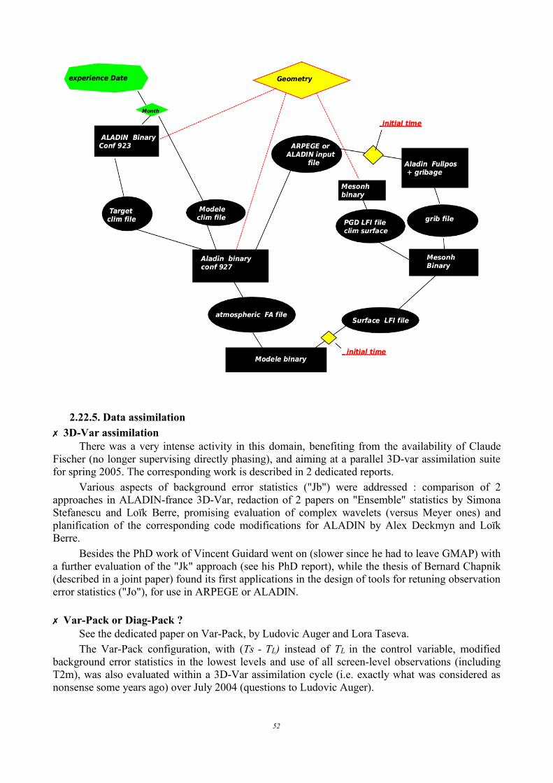
2.22.5. Data assimilation✗ 3D-Var assimilation

There was a very intense activity in this domain, benefiting from the availability of ClaudeFischer (no longer supervising directly phasing), and aiming at a parallel 3D-var assimilation suitefor spring 2005. The corresponding work is described in 2 dedicated reports.

Various aspects of background error statistics ("Jb") were addressed : comparison of 2approaches in ALADIN-france 3D-Var, redaction of 2 papers on "Ensemble" statistics by SimonaStefanescu and Loïk Berre, promising evaluation of complex wavelets (versus Meyer ones) andplanification of the corresponding code modifications for ALADIN by Alex Deckmyn and LoïkBerre.

Besides the PhD work of Vincent Guidard went on (slower since he had to leave GMAP) witha further evaluation of the "Jk" approach (see his PhD report), while the thesis of Bernard Chapnik(described in a joint paper) found its first applications in the design of tools for retuning observationerror statistics ("Jo"), for use in ARPEGE or ALADIN.

✗ Var-Pack or Diag-Pack ?See the dedicated paper on Var-Pack, by Ludovic Auger and Lora Taseva.The Var-Pack configuration, with (Ts - TL) instead of TL in the control variable, modified

background error statistics in the lowest levels and use of all screen-level observations (includingT2m), was also evaluated within a 3D-Var assimilation cycle (i.e. exactly what was considered asnonsense some years ago) over July 2004 (questions to Ludovic Auger).

52

Besides, Françoise Taillefer achieved the update of Diag-Pack to cycle 28T3, with problemsmet in the post-processing of the specific CAPE or MOCON fields.

✗ 3D-FGATBeside phasing, Cornel Soci further investigated the problem of significantly different

analysis increments between 3D-FGAT and 3D-Var, and costs issues too.First it was realized that backgrounds were not the same for the two analyses : a 6 h forecast

for 3D-Var, an integration based on 3 h, 6 h and 9 h forecasts for 3D-FGAT. Second, the initialexperimental framework was not consistent regarding physical packages.

A comparison based on the configuration of ALADIN-France assimilation gave thecorresponding figures for cost :- memory : 3D-FGAT only 1.3 times more expensive than 3D-Var if the trajectory is stored everytime-slot (i.e. every hour) instead of every time-step, - CPU : 3D-FGAT 8 times more expensive than 3D-Var, due to the calls to physics.

✗ Digital filtering- Optimisation of Digital Filtering in the ARPEGE 4D-Var

Here is a summary of the work performed by Adam Dziedzic, with help from FrançoisBouyssel, Gérald Desroziers and Dominique Giard, to evaluate the impact of the DFI constraints in(ARPEGE of course) 4D-Var on the spin-up of physics.

Digital filters (Lynch and Huang, 1992, Lynch et al 1997) are used twice in the ARPEGE 4D-Var. First, a Jc-DFI term is added, as a weak constraint, to the cost function (Gauthier and Thépaut,2000). DFI is also applied to filter the last analysed state in the incremental process, that includestwo minimizations each followed by a full-resolution update of the model trajectory. Because someimportant features of 4D-Var have changed since the implementation of DFI under that form, theaim of the present study was to check that the current use of DFI is still valid or at least welloptimised.

An ensemble of 4D-Var experiments have been performed in order to evaluate the optimalcombination of Jc-DFI and digital filtering of the last trajectory, called respectively inner and outerDFI hereafter.

A first set of experiments showed that incremental outer filtering (that is the presentoperational formulation) gives better results than non-incremental filtering, that tends to filter thefields too much.

The second set of experiments aimed at evaluating the impact of the use of the inner filteringperformed inside the minimization itself. In the operational configuration, the Jc-DFI constraint isapplied to all spectral fields (vorticity, divergence, temperature, humidity and surface pressure) andthis term is weighted by a factor that was tuned by Gauthier and Thépaut (2000). An increase of by a factor 5 (as in the operational implementation of Jc-DFI at ECMWF) slightly improves thespin-up at very short range but at the expense of a degradation of the fit of the analysis toobservations. Finally the application of the Jc-DFI to the divergence field only, with theamplification of the factor (as at ECMWF) did not show any particular improvement.

It has also been noted that the results obtained with and without outer DFI are very close butthat the spin-up at very short range is degraded when inner and outer DFI are removedsimultaneously. As a consequence, the conclusion of these different tests is that the presentARPEGE 4D-Var configuration in terms of DFI, including both inner and outer filtering, appearssatisfactory.Gauthier P. and J.-N. Thépaut, 2000 : Impact of the digital filter as a weak constraint in the pre-operational 4D-Var assimilation system of Météo-France, Mon. Wea. Rev., 127, 26-45.Lynch, P. and X.Y. Huang, 1992 : Initialization of the HIRLAM model using a digital filter. Mon. Wea. Rev., 120,

53

1019-1034.Lynch, P., D. Giard and V. Ivanovici, 1997 : Improving the efficiency of a digital filtering scheme for diabaticinitialization. Mon. Wea. Rev., 125, 1976-1982.

- Digital Filter initialization and ALADIN 3D-Var The impact of initialization on ALADIN 3D-Var assimilation was carefully studied by Claude

Fischer, and initial options reconsidered. See the paper on ALADIN-France 3D-Var.

✗ Observations- In ARPEGE, in short • From pre-processing to impact studies for satellite data (AMSUB, HIRS, AMSUA AQUA,

AIRS, QuickSCAT and MODIS winds, SSM/I, ...)• Introduction of a bias correction for radiosondes (from the IFS one)• Starting to work on GPS data

- Status and plans for developments on radar data The technical work required before addressing the problem of 4D-screening in ARPEGE /

ALADIN is now ended. Presently we have radar reflectivity data in ODB file and we have achievedthe main work to obtain a technical monitoring system for this observation type. In particular, a new subroutine (REFLSIM) is called within the vertical interpolation of modelfields, to compute and simulate the model-equivalent reflectivity at the observation point. Thisreflectivity observation-operator is an adaptation of the reflectivity simulator developed in theMeso-NH model. In particular the code organization does not allow horizontal integration as isrequired for radio-occultation data. However the vertical integration takes into account the radar-beam geometry, considering the radar-beam width at each observation point.

But in fact the physical interfacing is not satisfying and the required physical fields to simulatethe equivalent reflectivity are not easy to obtain. So, to start with 4D-screening, we have used thediagnostic cloudy parameters (liquid water and ice) computed by ARPEGE/ALADIN physics, andthe first trials show that most reflectivity data are rejected, due to too big obs-guess departures.According to this last point, the most important work is now to obtain the best required physicalfields in order to have a better first guess. A new observation-operator will be built, with snow, rainand graupel as input : diagnostic fields, derived from precipitation fluxes, in the case ofARPEGE/ALADIN, prognostic ones for AROME.

Moreover we have to optimize the thinning boxes and besides improve the quality control. Inparticular, the impact of the new quality flags provided by the CMR ("Centre de MétéorologieRadar"), stored in new radar BUFR and consequently in ODB, is to be evaluated. Maybe one couldalso improve screening by using a variational quality-control.

In parallel we intend to elaborate an inversion method, to provide some corrections of (T, q)profiles as retrievals from departures between the simulated and observed radar reflectivities.

✗ Else ?SEVIRI data in ALADIN : See the dedicated paper by Thibault Montmerle.Initialization of soil moisture : See the PhD reports of Karim Bergaoui.LAM EPS : See the paper bu Edit Hágel. Research on EPS is temporary in stand-by at Météo-France since Jean Nicolau is now too busy with other duties on top PEACE, while the RECYF teamis waiting for a new member to start such activities.

Hoping none is missing !

54

2.23. HUNGARY

As before our main areas of interest are data assimilation (3D-Var) and short-range ensembleprediction.

The brief summary of events can be presented as follows :• The application of new data types of the 3D-Var scheme was continued with the tests carried

out with AMDAR, wind profiler, SATOB and AMSU-B data. Most of the progress wasconcentrating on the development and improvement of data thinning algorithms for AMDARdata (a summary of results will be presented in the next Newsletter). The use of wind profilerdata was assessed and the control of their quality was investigated. SATOB winds (cloud-motion winds) were computed from METEOSAT-8 (MSG) data and used in the data ingestprocedure of 3D-Var. First trials were also taken by the pre-processing of AMSU-B data. It ishoped that all these developments together with some algorithmic improvements will lead toan overall improvement of the performance of the 3D-Var data assimilation scheme.

• Regarding our LAMEPS research and development we have further studied the sensitivity ofglobal singular-vector computations with respect to the target domain and target-time interval(a report from Edit Hágel can be read in the present Newsletter).

• In October-November, Miklos Voros spent 6 weeks at CHMI (Prague) to get familiar withALADIN-NH. The original topic proposed by Filip Vana was the correct definition of thebottom boundary condition (BBC) in order to eliminate chimney formation. Miklos had toprepare the ALPIA quasi-academic case to be a test-bed for the investigations. ALPIA, with itsdetailed orography but simplified atmosphere, represents a step between academic cases (e.g. asingle Bell-shape mountain, and uniform flow) and real case studies with realistic terrain andflows. On this testbed he was to study the effects of the semi-Lagrangian horizontal diffusion(SLHD) on the chimney effect. Finally, given the opportunity he had to test the interaction ofgravity-wave-drag (GWD) parameterization and SLHD. His work is yet unfinished and he willcontinue the job from Budapest.

• The dynamical downscaling of ECMWF ERA40 data was pursued on order to compute localwind climatology over Hungary. The length of the applied period was 10 years and a two-stepdownscaling was carried out : first to an intermediate 45 km resolution grid, then to a 15 kmmesh, and finally a short dynamical-adaptation post-processing was run at the final 5 kmresolution. Wind climatology was computed for 10 m, 25 m 50 m, 75 m, 100 m, 125 m and150 m heights.

2.24. MOROCCO: PROGRESS REPORT ON NUMERICAL WEATHER PREDICTION.

2.24.1. A brief summary of research development and main operational changesThe operational system consists of two parts :

ALADIN-NORAFThis configuration covers North Africa to the Equatorial belt with a resolution of 31 km. It is

used to provide NWP products to the ACMAD countries. In fact Morocco was engaged to produceforecasts over North Africa with a lower resolution than the other NWP models actually in use inthose countries. ALADIN-NORAF is also used to provide the boundary conditions to anoverlapping model ALBACHIR.

ALADIN-MAROC (ALBACHIR): Centred on Morocco with a finer resolution of 17 km, this model is used by local operating

services (short and medium range forecast, marine and aeronautic applications) and for otherproducts for specifics users.

55

The two NWP suites run on a super calculator IBM (RS/6000 SP). This machine is composedof three nodes with 36 processors of 1.5 GFPLOS each (54 GFLOPS on the whole).

In parallel to the work on the operational models ALADIN-NORAF and ALADIN-MAROC,the numerical prediction team carried out several research projects in the aim to validate the newsuite and to prepare futures changes. The main research projects in 2004 concern data assimilationmethods (3D-Var, BlendVar) and forecast error statistics (called Jb) computation. OSEs2 were alsocarried out in order to evaluate the impact of current observation systems and the contribution ofintroducing new ones (see part II for more details). A preliminary study on Ensemble PredictionSystem (EPS) has been achieved with the ALADIN-NORAF model.

2.24.2. Research and Development in data assimilation and numerical forecasting✗ Data assimilation methods

A study about data assimilation methods was carried out. The aim was to realize several dataassimilation cycles in order to single out the most adapted method to ALADIN-NORAF context.The first step was the running of a cycle based on 3D-Var.

Another data assimilation method called "blending" was tested in this study. The goal of thistechnique is to create an initial state combining the "large scales" resolved by the ARPEGE analysisto the "mesoscale" features provided by the short-range ALADIN forecast. Blending is consideredas a mesoscale data assimilation "without using observations". The last data assimilation methodtested (Blendvar) was a combination of blending and 3D-Var analysis. In this case the first guess for3D-Var analysis is created by the blending method. As main result, this study shows that Blendvarhas the best impact in analysis and forecast performance.

✗ Calculation of Jb termA -plane horizontal balance has been developed and coded for the Jb term of the ALADIN

3D-Var and for the associated software of error covariance calculations. In this study, instead oftaking ƒ (Coriolis parameter) constant over the ALADIN domain, the formulation is based on atruncated spectral expansion of the meridional variations of the Coriolis parameter. It can be seen asa multi-diagonal approach, in contrast with the purely diagonal approach of the ƒ-plane balance.This approach was first validated by examining, over the ALADIN-NORAF domain, the increase ofexplained variance when using the -plane balanced geopotential instead of the ƒ-plane balancedgeopotential. The formulation was then coded in the ALADIN 3D-Var, and it was validated using inparticular single-observation experiments.

✗ Installation of CY28T3 on IBM/RS6000No significant changes were operated on code since the mother calculator is an IBM, only few

changes in odb because of wrong interpretation of pre-compiler to the use of some characters asvariables or as directives.Hardware configuration :

The system is an RS/6000 SP with 54 GigaFlops composed of 3 nodes High (Night Hawk 2): - 2 nodes of 16 processors for calcul, - 1 node of 4 processors for file managing.

The processor is a Power 3-II with 375 Mhz and develop a power of 1.5 GigaFlops. Theglobal machine central memory is 19 Go. The masse memory (RAID 5 discs ) is 1019.2 Go

Software configuration :AIX 5.1 ML3, XLF 8.1.1.1, C compiler 6.0, ESSL, MASS, LoadLeveler 3.1.0.21

2 OSE : Observing System Experiment

56

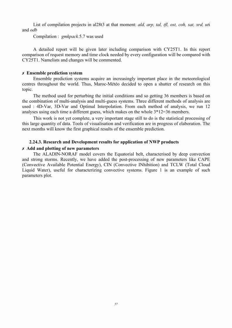
List of compilation projects in al28t3 at that moment: ald, arp, tal, tfl, ost, coh, sat, xrd, utiand odb

Compilation : gmkpack.5.7 was used

A detailed report will be given later including comparison with CY25T1. In this reportcomparison of request memory and time clock needed by every configuration will be compared withCY25T1. Namelists and changes will be commented.

✗ Ensemble prediction systemEnsemble prediction systems acquire an increasingly important place in the meteorological

centres throughout the world. Thus, Maroc-Météo decided to open a shutter of research on thistopic.

The method used for perturbing the initial conditions and so getting 36 members is based onthe combination of multi-analysis and multi-guess systems. Three different methods of analysis areused : 4D-Var, 3D-Var and Optimal Interpolation. From each method of analysis, we run 12analyses using each time a different guess, which makes on the whole 3*12=36 members.

This work is not yet complete, a very important stage still to do is the statistical processing ofthis large quantity of data. Tools of visualisation and verification are in progress of elaboration. Thenext months will know the first graphical results of the ensemble prediction.

2.24.3. Research and Development results for application of NWP products✗ Add and plotting of new parameters

The ALADIN-NORAF model covers the Equatorial belt, characterised by deep convectionand strong storms. Recently, we have added the post-processing of new parameters like CAPE(Convective Available Potential Energy), CIN (Convective INhibition) and TCLW (Total CloudLiquid Water), useful for characterizing convective systems. Figure 1 is an example of suchparameters plot.

57

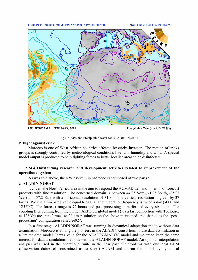
Fig.1: CAPE and Precipitable water for ALADIN -NORAF✗ Fight against crick

Morocco is one of West African countries affected by cricks invasion. The motion of cricksgroups is strongly controlled by meteorological conditions like rain, humidity and wind. A specialmodel output is produced to help fighting forces to better localise areas to be disinfected.

2.24.4. Outstanding research and development activities related to improvement of theoperational system

As was said above, the NWP system in Morocco is composed of two parts :✗ ALADIN-NORAF

It covers the North Africa area in the aim to respond the ACMAD demand in terms of forecastproducts with fine resolution. The concerned domain is between 44.8° North, -1.9° South, -35.3°West and 57.2°East with a horizontal resolution of 31 km. The vertical resolution is given by 37layers. We use a time-step value equal to 900 s. The integration frequency is twice a day (at 00 and12 UTC). The forecast range is 72 hours and post-processing is performed every six hours. Thecoupling files coming from the French ARPEGE global model (via a fast connection with Toulouse,at 128 kb) are transformed to 31 km resolution on the above-mentioned area thanks to the "post-processing" configuration called ee927.

In a first stage, ALADIN-NORAF was running in dynamical adaptation mode without dataassimilation. Morocco is among the pioneers in the ALADIN consortium to use data assimilation ina limited-area model. It was valid for the ALADIN-MAROC model and we try to keep the sameinterest for data assimilation methods with the ALADIN-NORAF model. An optimal interpolationanalysis was used in the operational suite in the near past but problems with our local BDM(observation database) constrained us to stop CANARI and to run the model by dynamical

58

adaptation. Observations were provided by the local observation database. However, there is aweakness in the conventional observations coverage, which has to direct us to the use of satelliteobservations. In this context, 3D-Var seems to be a more appropriate data assimilation method thanCANARI. Research work was carried out in this direction and put into concrete form in a doublesuite with 3D-Var data assimilation mode.

Some ALADIN-NORAF outputs (charts of meteorological parameters at several levels) areavailable via internet (see examples in Figs 2). Moreover, it is expected that, in a near future, GRIBfiles from the ALADIN-NORAF suite will be sent to ACMAD countries via a satellite RETIMconnection.

✗ ALADIN-MAROC (ALBACHIR )It is centred on Morocco with a resolution of 16.7 km. Vertical resolution is 37 layers.

Couplings files are provided by ALADIN-NORAF model. The initial state is that of ALADIN-NORAF transformed to the ALBACHIR domain tanks to the same procedure as used for couplingfiles : the ee927 configuration. GRIB files are produced every 3 hours and are transmitted to theoperating centre and to the four regional meteorological centres in Morocco for local use. 2.24.5. REFERENCEElouaraini, R., L. Berre, 2003 : Introduction of the -plane into the horizontal balance equation of ALADIN JbHdidou, F., C. Fischer, 2002 : Mise en place d’une chaîne d’assimilation pour ALADIN NORAF basée sur latechnique BlendvarSahlaoui, Z., E.Gérard, F.Rabier, 2002 : Assimilation of ATOVS raw radiances in ALADIN

59

Fig. 2: Some forecast fields of the ALADIN-NORAF model

2.25. POLAND

No news.

2.26. PORTUGAL

On the development side, new diagnostic tools have been under validation in order to becomeoperational. Those are : RISCON, thermal front parameter (TFP), and Q-Vectors. The diagnostictool RISCON, a composition of several parameters, provides a RISk of deep CONvection (from 0 to6) for a region by the combination of humidity in low levels, upward motion and instability. Thesevariables are inferred by numerical parameters derived from the model output fields: moistureconvergence in low-levels, vertical motion and/or Q-vector convergence and the indices Jeffersonand/or Total Totals and/or Convective Instability.

2.27. ROMANIA

2.27.1. The implementation of cycle 28T3 on SUN E4500 and Linux cluster platforms(Cornel Soci)SUN platform

The implementation has been performed using the explicit interfaces generated on VPP5000.Minor problems, specific to the SUN Forte 6 compiler, have been encountered.Linux cluster

The platform was designed and built in our institute. It is based on Intel XEON processor.

61

There are 6 nodes with 2 processors per node. The cluster is going to be upgraded with 6 morenodes.

ALADIN model was implemented using gmkpack, Intel compiler and mpich library. We aregrateful to Jure Jerman, Andrey Bogatchev, Ryad El Khatib and Stjepan Ivatek-Sahdan for theirkind support.

2.27.2. Dynamical adaptation of the wind using the ALADIN NH (Steluta Alexandru)See the report of Steluta Alexandru "High resolution dynamical adaptation of the wind

forecast using the non-hydrostatic version of the ALADIN model", in this Newsletter.

2.27.3. The flash flood event of 28th of August 2004 (Doina Banciu and Cornel Soci)On August 28 south-eastern Romania (Dobrogea and eastern part of Muntenia) was affected

by a Mediterranean origin cyclon evolving over the western basin of the Black Sea. The convectiveactivity intensified over the sea during the night of August 27/28. During the day, the intenseconvective cells coming from the sea towards the shore and after that onto the land generatedtornadic winds (waterspouts), intense electric activity, sporadic hail and an exceptional amount ofprecipitation: 190 l/m2 at Constanta (on the shore, cumulated in 12 h), 318 l/m2 at Pantelimon (inland, cumulated in 24 h).

The operational ALADIN (AL15) forecast indicated large areas of high precipitation in thesouth and north-eastern part of Romania but completely failed in predicting the severe weatherevent which occurred in the vicinity of the Black Sea coast.

For the case study two types of experiments have been carried out :• The operational integration domain (100×100×41, x=10 km) was enlarged (160×120×41)

for better covering the western basin of the Black Sea. • The horizontal resolution was increased up to 2.5 km for a domain covering only the south-

eastern Romania (216×216 points).For both series of experiments the non-hydrostatic version of the ALADIN model, cycle

28T3, was used. Another difference with respect to the operational suite was the usage of the lineargrid and the absence of orography envelope. For the experiments at 2.5 km the initial and boundaryconditions were provided by the simulations at 10km resolution (coupling frequency 3 hours).

The results showed that the precipitation amount was increased and the convective systemover the sea was more structured (especially for the simulation at 2.5 km) but there weredeficiencies in positioning of the precipitation cores. The case is still under study.

We would like to thanks to Radmila Brozkova for her advices in running the non-hydrostaticversion of the ALADIN model. and to Gwenaëlle Hello for providing us an AROME simulation forthis case.

2.27.4. The common ALADIN verification project (Simona Stefanescu)From this summer Romania has joint the common ALADIN verification program. The data extraction procedure, developed by the Slovenian colleagues has been installed on a

SUN workstation without any problem, using the PALADIN package. The surface and upper-airparameters forecasted by the ALADIN-Romania model for the established list of stations are sent bye-mail to Ljubljana to be inserted into the central database.

2.27.5. First test on EPS ALADIN-Romania (Mihaela Caian) a) The integration area (the coupling domain) was regionalized in sub-domains of similar

62

response to initial conditions perturbations; these sub-domains were identified computing abaroclinic instability diagnostic (the average rate of conversion of available potential energy of themean flow to eddy potential energy), maximal values indicating areas with increased potential formaximal perturbation growth. An example of the separation in sub-domains of response to initialconditions perturbations is shown in Figs 1 (showing the index at 850, 550, 300 hPa). Preliminaryresults indicate areas of maximal sensitivity in inner-Carpathian and SV regions in the lowertroposphere (as expected emphasizing with a westward tilt on the vertical). A maxima over theBlack Sea at higher levels shall be further analysed in connection with local diabatic sources. Thehigher troposphere is characterized by a mainly dipolar structure for the tested period, with a highersensitivity in the western region that will be also analysed further.

b) The use of SLAF (Scaled Lagged Average Forecast) method: the method is preliminaryused for 6 hours lag, leading to 2 to 4 ensembles with analysis as initial conditions, depending onthe comparison time; hourly ranges are compared and the error spread is analysed in connectionwith regions determined at a).

2.27.6. Verification of spectral coupling method on daily basis (Raluca Radu)A verification chain of spectral coupling is performed against operational ALADIN (cycle 15).

Daily and monthly scores fill daily a database for August 2004. The scale-sensitivity diagnostic toolis under development. In order to determine the impact of the spectral coupling scheme ontemperature and mean-sea-level (MSLP) fields, daily and monthly distribution scores (BIAS andRMSE) maps have been realized. The results are indicating generally, an increased forecastperformance when using spectral coupling.

63

Fig.1: Instability index at 850 (a), 550 (b) and 300 hPa (c)

64

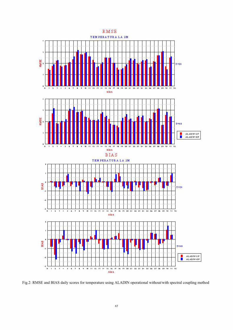
Fig.2: RMSE and BIAS daily scores for temperature using ALADIN operational without/with spectral coupling method

65

Fig.3: Monthly RMSE distribution for MSLP using ALADIN operational without/with spectral coupling method

66

2.28. SLOVAKIA

See the report on OPERATIONS.

2.29. SLOVENIA

2.29.1. Verification projectThe web interface for visualization of data, calculation and visualization of verification

scores, etc. is now accessible through internet. Authentification is not ready yet but anyoneinterested can ask for the address.

The verification system is still in testing mode (limited number of models, low performance)so currently we are receiving model data from 7 countries (Austria, Croatia, Hungary, Slovakia,Slovenia, Romania, Tunisia).

To solve the performance problems we tested various indexes on tables in PostgreSQLdatabase and their combination, but without significant success. We are getting much morepromising performances with computing differences for each model point and time slot against theobservation and storing them into new separate tables and using them for computations of allverification scores.

2.29.2. Testing of Latent Heat Nudging in ALADIN Model.Latent heat nudging (LHN) has been implemented in ALADIN model (cycle 25T1). With this

method the model is forced with measured precipitation rate. Measurement data are interpolated tomodel grid and combined with model precipitation values. Latent heat release part of temperaturetendency profile in the model is then rescaled with the ratio of observed and analysed precipitation.

LHN runs were performed for the entire year 2002. Measured precipitation data were usedfrom the 3 closest radars. Nudging was performed for the first twelve hours of the run and after thatthe model was left on its own. Generally there was only marginal positive effect for LHN runs. Insome cases a better spatial pattern of precipitation occurred. On the other hand there were someunrealistic cases of outbreaks of convection after the end of nudging period.

2.29.3. Probability forecast of temperature with quantile regression methodA probability forecasting can also be done with a statistical model and not only with the

ensembles. An advanced regression method, called quantile regression can be used as suchstatistical model. This method takes into account the true distribution of residuals, and combinesprobabilistic forecast and statistical adaptation of NWP direct model output variables to the localconditions. The result is not only the forecasted value but we also get the accuracy estimation of thisforecast. This method allows us to produce probabilistic forecast not only for discrete but also forcontinuous variables. For development of such statistical model the learning data set is needed, bigenough to train the model.

The quantile regression method was tested on maximum and minimum daily temperatureforecasts and 2 m temperature forecasts for different time ranges and for different locations inSlovenia. As predictors the observations and direct model output parameters from operationalALADIN model were used. With comparison of verification scores for quantile regression and someother regression methods it was shown that the weighted local linear principle is the most privilegedmethod among those tested.

2.29.4. High-resolution wind climatologyUsing an advanced numerical model is the best way for producing a physically consistent

67

spatially complete climatological field of surface wind. We produced datasets using severaldifferent configurations of ALADIN (single vs. double nesting, continuous in time vs. dynamicadaptation), all initialised and driven by ECMWF ERA-40 at the lateral boundaries. The horizontalresolution we are aiming at is 2.5 km using the ALADIN model and further down to 1 km using akinematic approach (mass-consistent model) or another dynamic model. In the next newsletter weare going to report on the results, i.e. which configuration appears to be the best for this purpose,and also present an objective verification of the obtained wind climatology.

2.30. TUNISIA

2.30.1. Changes in coupling files resolution as a solution to the transfer problemSince the first local implementation of ALADIN-Tunisie which is running on IBM Regata

platform, we used to receive coupling files from Toulouse at ALADIN-Tunisie resolution (12.5 km)via Internet connection in parallel to a leased line (64 kbits/s), but we registered too many problemsto get all the files at the expected hour (06:00 UTC) because of the big volume needed to betransferred in time with regard to the LS speed (about 140 Mo).

A first solution was to practice the so-called "asynchronous forecast", but the quality becamedebased.

The final solution adopted with the agreement of the DPREVI/COMPAS and GMAP teams isto transfer the coupling files at ARPEGE resolution (24 km). Hence, we have installed the requiredEE927 configuration after applying some changes on the operational cycle (Tunisia domain, climfiles, namelists and scripts). The work was done by ALADIN-Tunisie team.

A successful production test has been achieved by 23 November 2004 on 12:00 UTC run. Thechange to the new coupling files became operational since 24 November 2004 with 00:00 UTC run.This new configuration is running operationally without registered delay since that date.

2.30.2. Other events✗ Gmkpack 5.1

The gmkpack 5.1 version was adopted to manage and compile ALADIN export packages onthe IBM Regata platform of INM. This version was tested for the cycle 28T3 which was compiledsuccessfully.

✗ Configuration tests for cycle 28T3The configurations e927 and e001 were tested with success for the cycle 28T3. A validation

work will be done in immediate future.

✗ DiagPackA preliminary work was done for the installation of DiagPack on IBM Regata, this led to a

successful test of the surface optimal interpolation CANARI. The forthcoming work consists in:• Hourly integration of SYNOP data, • MOCON and CAPE computation for Full-Pos.

✗ VerifAladThe compilation and the implementation of the VerifAlad package in the operational regime

was done with success. Data to be verified and assessed are sent twice a day for the two networks ofthe day (00:00 and 12:00). Ten synoptic stations were chosen for a test period control.

68

3. ALADIN PhD Studies

3.1. Incrementality deficiency in ARPEGE 4d-var assimilation scheme: Radi Ajjaji: .

On temporary (?) leave from Maroc-Météo.

3.2. Scientific strategy for the implementation of a 3D-Var data assimilation scheme for adouble-nested limited-area model: Steluta Alexandru.

Writing a paper in parallel to operational duties at home (see the Romania R&D report and theadditional paper in this Newsletter).

3.3. Estimation and study of forecast error covariances using an ensemble method in aglobal NWP model: Margarida Belo-Pereira.

Trying to write a paper and the PhD report in parallel to operational duties at home.

3.4. Further Improvement of a Simplified 2D Variational Soil Water Analysis: K. Bergaoui.

An extensive validation of the 2D-Var method with observed precipitation increments wasperformed, examining in particular the response of the analysis increments and the total soil watercontent to a such correction. The effort is now put on the redaction of a paper summarizing the workperformed within the ELDAS project.

3.5. Evaluation of assimilation cycles in a mesoscale limited area model: Vincent Guidard.

3.5.1. Formalism: a very brief reminderMore details in the Newsletter 26 issue. To input an information about the larger scales of the ARPEGE analysis in the ALADIN 3D-

Var, a new term is added in the cost function: J x=J b xJ o x 1

2 dk−H 2 x T V−1d k−H 2 x ,

where d k=H 1 x AA−H 2 xb is the innovation vector with respect to the larger scales of theARPEGE analysis, and V the error covariance matrix related to this source of information.

3.5.2. Evaluation over a 15-day period✗ Experimental framework

The evaluation is performed over a period from the 1st to the 15th of June 2004.- Datasets

In order not to use the same observations in ALADIN 3D-Var as in ARPEGE 4D-Var, twodatasets have been prepared. The first one is composed of all the observations outside the ALADIN-France domain plus a random half of the observations inside the ALADIN-France domain. Theother half of the observations inside the ALADIN-France domain is the second dataset. Thus anARPEGE assimilation cycle and its subsequent coupling files have been recomputed.

- Error Covariances Statistics The ''lagged NMC'' statistics are used for B (Široka et al., Meteor. Atmos. Phys., 2003).The ensemble evaluation described in the previous Newsletter is used for V.

- Experiments Our reference experiment is a ''classical'' ALADIN 3D-Var, i.e. a ''Jb+Jo'' 3D-Var, hereafter

69

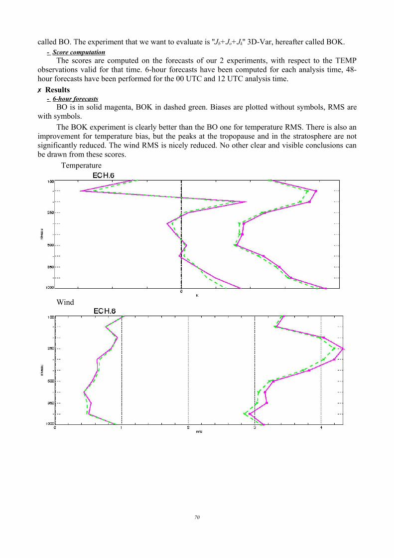
called BO. The experiment that we want to evaluate is ''Jb+Jo+Jk'' 3D-Var, hereafter called BOK.- Score computation

The scores are computed on the forecasts of our 2 experiments, with respect to the TEMPobservations valid for that time. 6-hour forecasts have been computed for each analysis time, 48-hour forecasts have been performed for the 00 UTC and 12 UTC analysis time.✗ Results

- 6-hour forecasts BO is in solid magenta, BOK in dashed green. Biases are plotted without symbols, RMS are

with symbols.The BOK experiment is clearly better than the BO one for temperature RMS. There is also an

improvement for temperature bias, but the peaks at the tropopause and in the stratosphere are notsignificantly reduced. The wind RMS is nicely reduced. No other clear and visible conclusions canbe drawn from these scores.

Temperature

Wind

70

Humidity

- Time evolution of the scores Vertical levels in ordinates, forecast range in abscissa. Green: BOK better than BO, Red: BOK worse than BO

Temperature

71

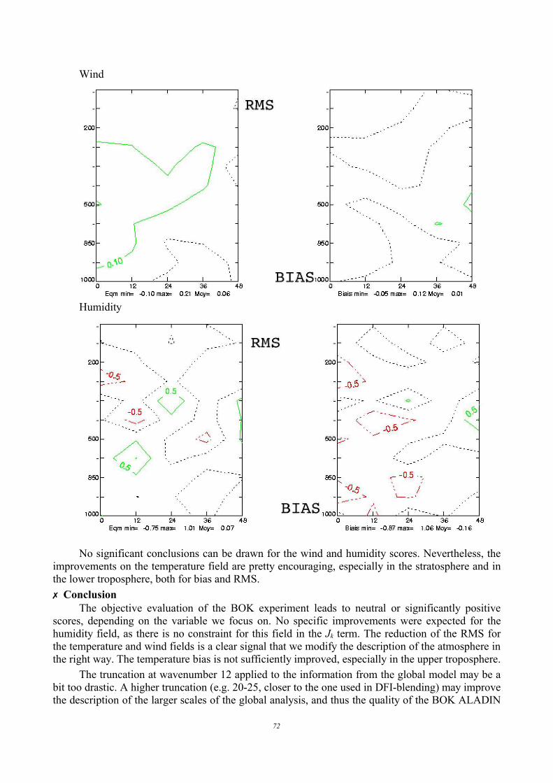
Wind

Humidity

No significant conclusions can be drawn for the wind and humidity scores. Nevertheless, theimprovements on the temperature field are pretty encouraging, especially in the stratosphere and inthe lower troposphere, both for bias and RMS. ✗ Conclusion

The objective evaluation of the BOK experiment leads to neutral or significantly positivescores, depending on the variable we focus on. No specific improvements were expected for thehumidity field, as there is no constraint for this field in the Jk term. The reduction of the RMS forthe temperature and wind fields is a clear signal that we modify the description of the atmosphere inthe right way. The temperature bias is not sufficiently improved, especially in the upper troposphere.

The truncation at wavenumber 12 applied to the information from the global model may be abit too drastic. A higher truncation (e.g. 20-25, closer to the one used in DFI-blending) may improvethe description of the larger scales of the global analysis, and thus the quality of the BOK ALADIN

72

analysis.

3.6. Interaction between physical processes: cloud life cycle, cloud transient states: Jean-Marcel Piriou.

The PhD work is now achieved and the report ready. Here is the extended summary :The present PhD work focuses on convection parameterizations for use in GCMs or regional

models. Firstly, a diagnostic study of the ARPEGE global NWP model was carried out: (i)comparing single column predictions versus 3D high resolution models (ii) studying the diurnalcycle of the 3D model: local solar time of precipitation maxima or cloud vertical extent.

Secondly, a review of articles about convection phenomenology and parameterization is done.The concept of BCC (Bulk Convective Condensation rate) is introduced to remove the chicken andeggs dilemma, in convective parameterization causality.

It is shown that (i) the humidity convergence cannot be used alone for dimensioning theconvective activity within the present parameterization (ii) the hypothesis of an uniform detrainmentcoefficient has to be relaxed to make the deep parameterization scheme relevant not only for wetcases, but also for drier mid-atmospheric ones or in the vicinity of non-precipitating convectivestates.

Finally, a new convective scheme is introduced, whose formalism can handle dry, non-precipitating or precipitating convection. (i) The updraft ascent scheme deals explicitly with in-cloud condensates (liquid or ice), adjustment and auto conversion (ii) large-scale equations areexpressed directly in micro-physics and transport terms (iii) the closure can shift continuously froma CAPE behaviour to a humidity convergence behaviour (iv) a diagnostic in-cloud vertical velocityis used to determine cloud extent and penetrative updrafts. The results show the relevance of aconvective parameterization directly expressed in terms of micro-physics and transport, i.e. Upsteam Yanai and al. 1973.

The present work thus deals with three convection-related topics: phenomenology,parameterization, validation of parameterization results.

3.7. Extensive study of the coupling problem for a high-resolution limited-area model:Raluca Radu.

Further validation of the new method : see the Romanian contribution to research anddevelopments.

3.8. A posteriori verification of analysis and assimilation algorithms and study of thestatistical properties of the adjoint solutions: Wafaa Sadiki.

Defence scheduled for April 7th !

3.9. Study of the relationship between turbulent fluxes in deeply stable PBL situations andcyclogenetic activity: André Simon.

Work is still focussing on the study of the relationship between turbulent fluxes andcyclogenesis. The present study (or, better to say, what was studied in Toulouse) is more related toparameterization of the mixing length of momentum with respect to Ekman friction. See the stayreport for more details.

73

3.10. Systematic qualitative evaluation of high-resolution non-hydrostatic model: KlausStaldbacher.

See the Austrian contribution to research and developments.

3.11. The modelling of the forecast error covariances for a 3D-Var data assimilation in anatmospheric limited-area model: Simona Stefanescu.

Continuing the work started in 2003, the experimental comparison of the ensemble approachwith the standard and lagged NMC methods, regarding the estimation of the error statistics for theALADIN 3D-var data assimilation, has been carried out. It was found that the error spectra providedby the ensemble method are intermediate between those of the two other methods.

The differences with respect to the representations of the analysis step and of the involvedforecast ranges have been studied. The analysis equation appears to be the equation that transformsthe background and observation errors into the analysis errors. In the ensemble technique, theanalysis step is also represented by the application of the analysis equation, which transforms thebackground and observation perturbations into the analysis perturbations.

In the standard NMC method, the representation of the analysis step consists in adding someanalysis increments to some evolved earlier increments, instead of applying the analysis equation tosome background and observation perturbations. It appears moreover that the analysis incrementspectrum is much larger scale than the analysis dispersion spectrum. These increment structures,their accumulation and the forecast evolutions contribute therefore to the enhancement of the large-scale variances in the NMC method, compared with the ensemble approach.

The ensemble technique has also been compared with the so-called lagged NMC method. Thelinks between the implied forecast differences and the ARPEGE/ALADIN model differences havebeen illustrated. The larger amplitude of the ensemble large-scale variances, compared to the laggedNMC method, may be explained by the representation (in the ensemble approach) of the initialcondition uncertainties and of the associated lateral boundary conditions uncertainties.

Two papers realized in collaboration with Loïk Berre and Margarida Belo Pereira have beenfinalized and submitted to Monthly Weather Review and Tellus:Stefanescu, S. E., L. Berre and M. Belo Pereira : The evolution of dispersion spectra and the evaluation of modeldifferences in an ensemble estimation of error statistics for a limited area analysis. Submitted to Mon. Wea. Rev.Berre, L., S. E. Stefanescu and M. Belo Pereira : A formal and experimental comparison between an ensembleestimation of limited area model error statistics and two other error simulation methods. Submitted to Tellus.

3.12. .Use of IASI/AIRS observations over land: Małgorzata Szczech-Gajewska.

Welcome to Alicja, born on October 30th !

3.13. Application of the Predictor-Corrector Method to non-hydrostatic dynamics: J.Vivoda.

The writing of a common reference article about the NH dynamics of ALADIN has started atthe end of reported period. I will contribute to it with the results of idealized and real case studies asa co-author.

3TL predictor/corrector scheme with Eulerian advection treatment has been coded andvalidated and actually pre-phased into main branch. It will be available for ALADIN communityfrom cycle 29T2. Also the grid-point semi-Lagrangian advection of vertical velocity, implementedwith NH prognostic variables d3 and d4, will enter cycle 29T2.

74

3.14. A survey on well-posed and transparent lateral boundary conditions (LBCs) inspectral limited-area models: Fabrice Voitus.

The "flow relaxation" scheme of Davies (1976) is presently the technique the most widelyused for treating the lateral boundaries. It consist in defining a "relaxation zone" next to theboundary within which all the prognostic fields are relaxed toward the externally supplied "hostmodel" fields (being understood, as in McDonald (2000), as the model supplying the boundariesfields for the limited-area "guest model"). Despite its almost universal use in operational limited-area numerical weather prediction model, the "flow relaxation" scheme has still some unavoidableweaknesses. Over-specification implies that the problem to be solved is ill-posed : we impose fieldsat the boundary which are not strictly necessary from the point of view of the inwardlycharacteristics velocities (see Oliger and Sundström, 1979, for details). Moreover, because of thedifficulty to determine a suitable width for the boundary relaxation zone (see Kallgerg 1977), thetreatment of the boundary is not fully transparent and can generate spurious gravity waves whichpropagate back into the domain. In order to circumvent these weaknesses, McDonald (2000, 2002,2003) propose an elegant alternative to the flow relaxation scheme in the (grid-point) HIRLAMmodel using a C-grid finite-difference scheme. His new LBCs treatment removes the idea of arelaxation zone by imposing the host model fields on the boundary line only (as it's mathematicallyrequired) and tries to reduce false wave reflections at boundaries to a minimum while maintainingwell-posednesses, as suggested by the theoretical work of Engquist and Majda (1977).

The main object of this study is to try to transpose McDonald's idea to the case of spectrallimited-area models (Haugen and Machenhauer 1993). The last months have been essentiallydevoted to bibliography and to the implementation (as properly as possible) of the well-posedtransparent boundary condition derived by McDonald (2000) into a linear spectral 1D shallow-watermodel. In the spectral model based on Haugen-Machenhauer solution, before the use of fast Fouriertransforms (FFT) in the horizontal direction, the fields are extended into a meteorologicallymeaningless so called "Extension zone" (hereafter E-zone) outside the integration area (hereafter C-zone) in such a way that periodic fields are obtained. Given the field in the C-zone, the values set inthe E-zone result from a purely mathematical operation performed by means of a linear splineoperator. The coupling is now performed only at the boundary of the C-zone, at the beginning of thetime-step.

A first attempt has been made by Termonia (2003) who has found encouraging results for a2TL-SISL discretization, when small time-steps are used. Termonia has shown that the periodicspline operator should be apply at each time-step to ensure consistency of solution over the C-zone.However, this procedure is too expensive, for the while, to be intensively used. That means thatwell-posed and transparent LBCs in a spectral model of Haugen-Machenhauer type suppose that wepay a special attention to the "E-zone". In the continuation of Termonia's experiments, we haveimposed the characteristic fields at boundaries and observed that this LBCs give satisfactorytransparency condition, (there are still spurious reflections, but with acceptable amplitudes).Unfortunately, further experiments with larger time-steps, such as those usually allowed by thesemi-implicit semi-Lagrangian time-stepping, lead to computational instabilities. For now, it isdifficult to identify the cause of such an instability, but we remain optimistic.

75

4. PAPERS and ARTICLES

4.1. Some informal news from the AROME project: F. Bouttier, G. Hello, S. Malardel, Y.Seity, with help from many others.

This paper presents an overview of the design choices of AROME and an update on the statusof its development. 4.1.1. Objectives

The basic reason for making AROME is to get ready for the next generation of computers,observations and users' requirements, by taking the best of what is already available – ALADIN-NHdynamics and software basis, some physics that are guaranteed to work well at kilometric scales, theIFS/ARPEGE/ALADIN variational analysis – and putting it together as a newer, better operationalsystem. Over ten years of experimentation in the mesoscale research communities have given strongindications that it is a realistic goal, at least, for the most important aspects: much improvedprecipitation forecasts than in ALADIN. The choice of ALADIN-NH dynamics and ALADIN-3DVar to do AROME is a tribute to the excellent work of many ALADIN scientists whocontributed to these projects, as confirmed by the many peer-reviewed publications on theirscientific content.

The same software basis in AROME as in ALADIN – the IFS/ARPEGE library – is used,which provides a guarantee that there will only be minimal disturbances to the partners' operationalpractices. Only a small amount of technical adaptation will be required on the partner NWP servicesto switch to AROME when they want to start using it. In the meantime, ALADIN will keep running(and improving through the work done on improving its big brother ARPEGE), and ALARO willprovide a much improved alternative to ALADIN for those who cannot switch to AROME.

4.1.2. Using the Méso-NH physics The choice of the complex Méso-NH physics (compared to the ARPEGE/ALADIN physics)

was driven by the user requirements to improve products such as quantitative precipitations, small-scale convective rain and gusts, 3D distribution of cloud ice and water, aircraft icing and turbulencerisk, urban weather and air quality, accidental pollutant dispersion, road conditions, coastal weather,fluxes for ocean models. Since the Méso-NH physics already are in a usable state, the priority ofAROME is the software engineering and qualification for NWP applications, to be done in a fixedtime.

As models go to higher resolutions, more subgrid-scale processes are explicitly resolved onthe model grid. The AROME physics only borrows from Méso-NH the parametrizations that havebeen proved to be of significant importance at 2.5km resolution in Méso-NH experiments (thechoice is confirmed by other NWP groups):

• a 1-D (i.e. vertical) prognostic turbulent mixing scheme• a 1-D state-of-the-art radiation scheme• a cloud micro-physics scheme that separates at least between liquid water and ice, and

between small cloudy particles and bigger hydro-meteors• the best affordable surface scheme, consistent with the available physiographic databases• a shallow convection scheme

The schemes have been thoroughly validated in a large number of Méso-NH tests: convectivestorms, hurricanes, synoptic storms, PBL city weather, field experiments such as PYREX and MAP,and many more. There are some changes with respect to the ALADIN philosophy: the surfacescheme has explicit time-stepping (not a problem with the AROME time-step, which is muchshorter than in ALADIN), the vertical discretization is different, the surface scheme is externalised,

76

and the coding rules, but are a bit different from the ALADIN ones. It was found more efficient toadapt to this new physics software than to rewrite it; an abundance of documentation, peer-reviewedpublications and scientific experts is available on the Méso-NH physics.

The vertical turbulent scheme is based on a turbulent kinetic energy closure. It is prognostic,which should help with the depiction of the evolution of boundary layers and clouds. It isscientifically very close to what is being implemented in ARPEGE/ALADIN in 2005 at GMAP(although the code itself is still different). For very high resolutions, theory tells that the turbulentscheme should be a 3D one (i.e. elaborate horizontal mixing), however this effect seems to besignificant only at resolutions higher than 1km, 3D turbulence is very complex and expensive, andthe parametrization is still far from being in a satisfactory state, so it was decided to stick with a 1Dscheme for the next few years.

The radiation scheme is very important for cloud/radiation interaction, and for the productionof accurate fluxes at the surface (which is critical for some users). Since it is a lot of work todevelop a competitive radiation scheme, it was decided in Méso-NH (and hence in AROME) to usea recent version of ECMWF's radiation scheme, RRTM, which happens to be already convenientlyinstalled in the ARPEGE/ALADIN code.

The cloud micro-physics scheme (called ICE3, because it has three prognostic icy variables,on top of 2 liquid water ones) is scientifically very complex, and deals separately with theconversion («slow») processes, and the ones related to precipitation and saturation («fast» andadjustment). Condensed water species do not have special prognostic temperature or speed, but theyinteract with the gaseous thermodynamics in complex ways.

The surface scheme is derived from the ISBA we know in ALADIN, but now, with manymore processes, since it now includes tiling (i.e. several different surfaces may coexist in eachmodel column, each with their own surface temperature), prognostic models for towns (with aspecial geometry for walls, roofs and streets, to represent urban heat island effects in particular),lakes, snow, and soon superficial ocean layers (so-called 1D «pseudo-3D» mixed layer).Technically, the really difficult issue is that it means dozens of new surface fields (physiographicand prognostic) in the system. It is no longer necessary to allocate them inside the ALADINsoftware (because they belong to the surface software, called SURFEX) but plugging these newfields inside our NWP technical environments is going to be a significant challenge: one will need,either to manage the model history as two files (one for the ALADIN atmosphere, one for theSURFEX state), or to define, allocate and maintain all these new 2D fields (as well as some non-2Ddata, there are coefficients and matrices) into the FA files. Fortunately, SURFEX already has acomplete environment for computing climate files from high-resolution physiographic databases(the ECOCLIMAP database), doing I/O on SURFEX files and producing diagnostics.

The shallow convection scheme is not yet finalized, and work will be done on this topic in2005.

This physics package will have its own problems. All convection is not resolved horizontallynor vertically at a resolution of 2.5km and L41 levels. Some of the turbulent eddies are partlyresolved, which may cause problems akin to the subgrid convection issue in 10-km resolutionmodels. Some of the cloud physics are missing, which may hurt the description of some cloud types.They may not be serious issues in practice, but they need to be carefully monitored on a goodenough sample of real test cases, because they might lead to an evolution of the scientific strategy.The Méso-NH group keeps working in this field, on chosen test cases to target specific processes, itis necessary to complement this effort by looking at NWP-style validation, with lots of unselectedcases, and a global view of the performance of the AROME model.

4.1.3. The state of the prototypeUpon examination, it turned out not to be too complicated to plug the Méso-NH physics into

77

AROME. Yann Seity and Sylvie Malardel produced a first working version of the so-calledAROME prototype in just a few months (the word "prototype" means that it is a bread-board testbedthat needs to evolve into a clean and efficient configuration). Basically, the relevant Méso-NH andSURFEX source code has been extracted as libraries, and linked with the ALADIN-NH codethrough a specific physics interface (APLAROME) beside APLPAR. Although the timetable of theAROME project will not allow too ambitious plans for redesigning the physics interfacing from atheoretical and technical point of view, significant improvements can and will be done under theconstraint of the available workforce.

The first step for AROME was to prove that it could compete with Méso-NH in terms ofquality and cost. This required some Méso-NH-style testing on simplified cases: the dry ALADIN-NH dynamics on low-level orographic waves (already presented a few years ago), 1D simulation ofconvective and stratiform clouds (using the 1D model with physics), 2D vertical plane simulation ofa convective system (an idealized African squall line), 3D simulation of an idealized convectivecloud. All these tests revealed differences between AROME and Méso-NH, but no spuriousbehaviour of AROME.

The first real test cases were run in 2004. Each one required some considerable manual work,due to the technical nature of the prototype. There has been one famous convective flood event inthe SE of France (the "Gard case"), and a thunderstorm system on the plains around Paris. On bothcases, it was demonstrated that the AROME prototype was

1. performing at least as well as Méso-NH (although there is room for improvement ofAROME),

2. sensitive, in a positive sense, to the assimilation, by checking that an AROME run startedfrom a mesoscale analysis does indeed perform much better than one in purely dynamicaladaptation mode (which justifies the current effort on developing mesoscale dataassimilation).

3. much more efficient than Méso-NH in a CPU sense (by a factor 10 or so), thanks to its longerfeasible time-step (which could be stretched to 1 minute, which remains to be confirmed on awider panel of cases), and not more expensive than what is affordable, computerwise, atMétéo-France in 2008 (which looks like a realistic goal so far).

To obtain these results was a huge relief. Although they do not prove that AROME is matureenough to be safely used in operations, they go a long way towards proving that, even thoughunexpected problems with probably be discovered in AROME in the future, they will be tractable. Italso proved that it was feasible to work in a mutually beneficial cooperation between the Méso-NHresearch groups and the NWP community.

The work on the «old» ALARO model concept (i.e. AROME + convection scheme running at5, 7 or 10km resolution) has been interesting for the comparison with AROME, too. It was mainlydone by G. Hello, T. Kovacic, L. Kullman, who ran the Gard case (and a «Czech front» case) atvarious resolutions. It showed that the Méso-NH physics can work at larger scales and longer time-steps, although it has not been proven to beat the ALADIN physics at low resolutions.

Further test-cases are being worked on. There has been a case on Romania, on the MAP fieldexperiment (see figure), and more are planned, usually involving ALADIN partners or scientificvisitors. The results will be shown to the ALADIN community, of course. But there is a limit to theusefulness of test-cases for NWP, and it will soon be time to start running AROME every day (on asmall domain for computational reasons, until the next computer upgrade) in order to test whatAROME is worth in terms of robustness (does it ever blow up or produce silly forecasts ?) andaverage NWP performance (we have worked a lot on convection in AROME, but what about theother kinds of weather ?).

78

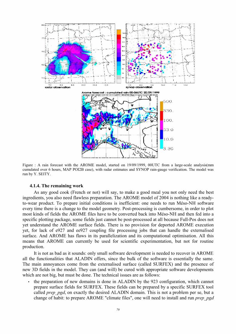
Figure : A rain forecast with the AROME model, started on 19/09/1999, 00UTC from a large-scale analysis(mmcumulated over 6 hours, MAP POI2B case), with radar estimates and SYNOP rain-gauge verification. The model wasrun by Y. SEITY.

4.1.4. The remaining workAs any good cook (French or not) will say, to make a good meal you not only need the best

ingredients, you also need flawless preparation. The AROME model of 2004 is nothing like a ready-to-wear product. To prepare initial conditions is inefficient: one needs to run Méso-NH softwareevery time there is a change to the model geometry. Post-processing is cumbersome, in order to plotmost kinds of fields the AROME files have to be converted back into Méso-NH and then fed into aspecific plotting package, some fields just cannot be post-processed at all because Full-Pos does notyet understand the AROME surface fields. There is no provision for deported AROME executionyet, for lack of e927 and ee927 coupling file processing jobs that can handle the externalisedsurface. And AROME has flaws in its parallelization and its computational optimisation. All thismeans that AROME can currently be used for scientific experimentation, but not for routineproduction.

It is not as bad as it sounds: only small software development is needed to recover in AROMEall the functionalities that ALADIN offers, since the bulk of the software is essentially the same.The main annoyances come from the externalised surface (called SURFEX) and the presence ofnew 3D fields in the model. They can (and will) be cured with appropriate software developmentswhich are not big, but must be done. The technical issues are as follows:

• the preparation of new domains is done in ALADIN by the 923 configuration, which cannotprepare surface fields for SURFEX. These fields can be prepared by a specific SURFEX toolcalled prep_pgd, on exactly the desired ALADIN domain. This is not a problem per se, but achange of habit: to prepare AROME "climate files", one will need to install and run prep_pgd

79

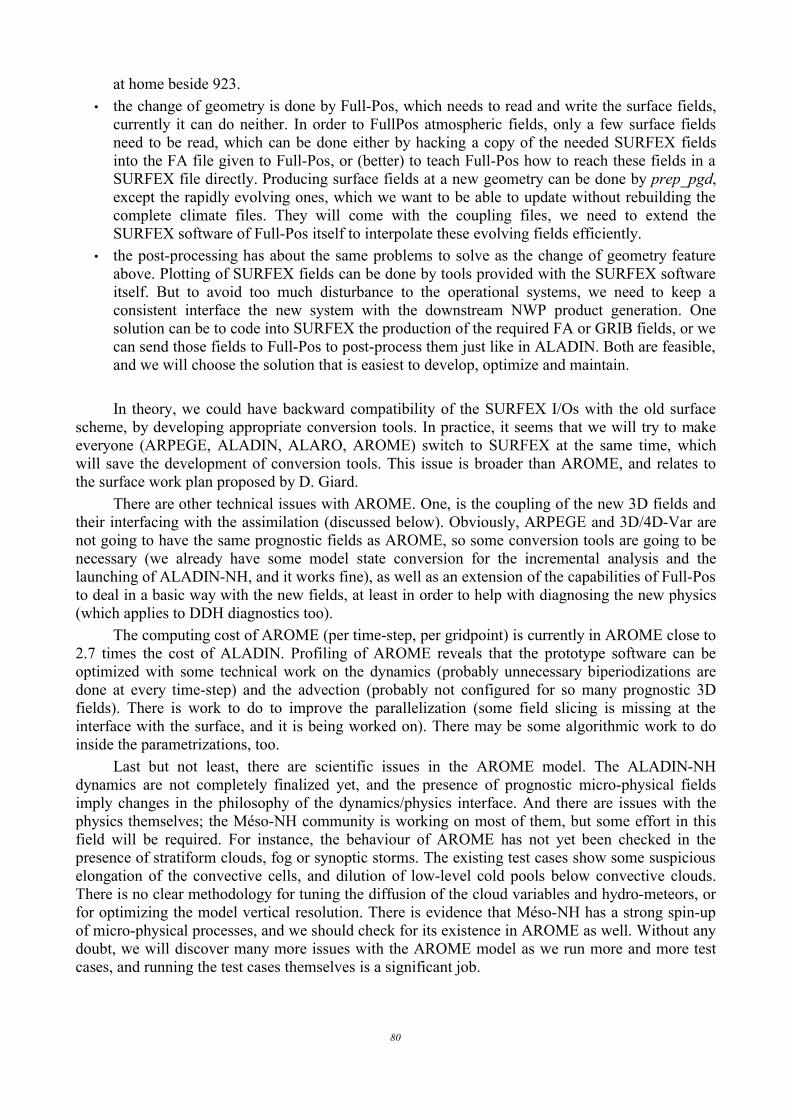
at home beside 923.• the change of geometry is done by Full-Pos, which needs to read and write the surface fields,

currently it can do neither. In order to FullPos atmospheric fields, only a few surface fieldsneed to be read, which can be done either by hacking a copy of the needed SURFEX fieldsinto the FA file given to Full-Pos, or (better) to teach Full-Pos how to reach these fields in aSURFEX file directly. Producing surface fields at a new geometry can be done by prep_pgd,except the rapidly evolving ones, which we want to be able to update without rebuilding thecomplete climate files. They will come with the coupling files, we need to extend theSURFEX software of Full-Pos itself to interpolate these evolving fields efficiently.

• the post-processing has about the same problems to solve as the change of geometry featureabove. Plotting of SURFEX fields can be done by tools provided with the SURFEX softwareitself. But to avoid too much disturbance to the operational systems, we need to keep aconsistent interface the new system with the downstream NWP product generation. Onesolution can be to code into SURFEX the production of the required FA or GRIB fields, or wecan send those fields to Full-Pos to post-process them just like in ALADIN. Both are feasible,and we will choose the solution that is easiest to develop, optimize and maintain.

In theory, we could have backward compatibility of the SURFEX I/Os with the old surfacescheme, by developing appropriate conversion tools. In practice, it seems that we will try to makeeveryone (ARPEGE, ALADIN, ALARO, AROME) switch to SURFEX at the same time, whichwill save the development of conversion tools. This issue is broader than AROME, and relates tothe surface work plan proposed by D. Giard.

There are other technical issues with AROME. One, is the coupling of the new 3D fields andtheir interfacing with the assimilation (discussed below). Obviously, ARPEGE and 3D/4D-Var arenot going to have the same prognostic fields as AROME, so some conversion tools are going to benecessary (we already have some model state conversion for the incremental analysis and thelaunching of ALADIN-NH, and it works fine), as well as an extension of the capabilities of Full-Posto deal in a basic way with the new fields, at least in order to help with diagnosing the new physics(which applies to DDH diagnostics too).

The computing cost of AROME (per time-step, per gridpoint) is currently in AROME close to2.7 times the cost of ALADIN. Profiling of AROME reveals that the prototype software can beoptimized with some technical work on the dynamics (probably unnecessary biperiodizations aredone at every time-step) and the advection (probably not configured for so many prognostic 3Dfields). There is work to do to improve the parallelization (some field slicing is missing at theinterface with the surface, and it is being worked on). There may be some algorithmic work to doinside the parametrizations, too.

Last but not least, there are scientific issues in the AROME model. The ALADIN-NHdynamics are not completely finalized yet, and the presence of prognostic micro-physical fieldsimply changes in the philosophy of the dynamics/physics interface. And there are issues with thephysics themselves; the Méso-NH community is working on most of them, but some effort in thisfield will be required. For instance, the behaviour of AROME has not yet been checked in thepresence of stratiform clouds, fog or synoptic storms. The existing test cases show some suspiciouselongation of the convective cells, and dilution of low-level cold pools below convective clouds.There is no clear methodology for tuning the diffusion of the cloud variables and hydro-meteors, orfor optimizing the model vertical resolution. There is evidence that Méso-NH has a strong spin-upof micro-physical processes, and we should check for its existence in AROME as well. Without anydoubt, we will discover many more issues with the AROME model as we run more and more testcases, and running the test cases themselves is a significant job.

80

4.1.5. Computational cost issuesThe debate about installing AROME in ALADIN countries is completely dependent on the

speed of their future computers. Assuming constant funding of NWP computers in each country, it isa safe hypothesis that the power of affordable computing for regional modeling is going to increaseat the same speed as in recent years: a doubling every 18 months. This is a result of currenttechnology progress called Moore's law: one person's increase in affordable computing will be 60%in 1 year, a factor 4 in 3 years, 16 in 6 years. That is to be compared with the cost of AROME:dx=dy=2.5km, dt=7min, the cost per gridpoint per time-step is 3 times that of ALADIN (which is asmuch due to the extra 3D fields required by the micro-physics, TKE and the NH dynamics, as to thecost of the physics themselves, by the way). Bringing together Moore’s law and the cost ofAROME, there can be two extreme point of views (and of course an infinity of intermediate views):

• The pessimistic view: I have an ALADIN at 10-km resolution and 7-min time-step. And I willnot use AROME until Moore’s law gives me a computer to replace ALADIN with the samedomain, forecast ranges, number of forecasts per days. That means AROME needs an(approximately) 4x4x7x3=300 computer increase, which Moore’s law will give me in 12years, that is, in 2012.

• The optimistic view: I have an ALADIN at 7-km resolution and 5-min time-step, runs to 48-hrange, and I believe current optimization work on AROME will bring the per-gridpointoverhead from 3 to 2.5. My ALADIN domain and forecast ranges are ludicrously oversizedfor AROME which is going to be primarily useful in the 0-24h forecast range; for longerranges I can keep running my good old ALADIN model or the brand-news ALARO model. SoI can shrink the AROME area to 20% of my current ALADIN domain, which covers theimportant areas of my country, and to half of my previous range. That means a computerincrease of 3x3x2.5x0.2x0.5=2.25; adding 1 to the cost to keep running ALADIN, the totalpower needed is 3.25. Applying Moore's law since the last time my boss bought me a newcomputer, say 2 years ago, means that AROME is affordable for me by the end of 2005.As one can see, the key aspects fo the AROME expense are not the AROME physics cost, but

the required domain size, useful forecast ranges, and current ALADIN resolution. Each partnershould consider its own options carefully. To try to replace ALADIN completely with AROME todo the same thing will not be an optimal approach for short-range, regional modelling. ALARO willprobably be more suited for NWP over wide areas.

4.1.6. Assimilation, predictability and couplingThe bulk of so-called AROME activities in Météo-France are on developing the model.

However, data assimilation is very important, because it is known (from the mesoscale scientificliterature of e.g. NCAR and from Méso-NH initialization impact studies since 1997) that dataassimilation gets more and more important as the resolution increases. This is mainly because deepconvective systems have interesting memory properties: the regional assimilation of low-levelfields, cloud fields and humidity has a substantial beneficial impact on mesoscale forecasts for atleast the first 12 hours, at constant large-scale forcing. Of course, it is important to improve thelarge-scale forcing too, but the novelty is that there is an enormous amount of unused mesoscaledata in many regions, whereas all the easy large-scale data is already being used in the global dataassimilation system. The other good news is that the most important part of the regional dataassimilation system can be setup regardless of the model: the ALADIN 3D-Var can be applied withvery few changes to ALADIN itself, to ALARO, AROME, or even Méso-NH. The importantdifferences are in the computation of the background term Jb (it requires different ensembles andsome fiddling of the variances), the data thinning (adapted to each model's resolution) and in theinterface between 3DVar and the forecast model (using the incremental approach: 3DVar analyseswind, T and q, it is useful to correct them in all models). Thanks to the excellent work of theALADIN scientists, Météo-France has been able to set up a pre-operational 3DVar for ALADIN

81

and Méso-NH relatively quickly, and AROME and ALARO will follow soon.To go to higher resolution, a few extras will need to be put into 3DVar, starting with those

with the best cost/benefit ratio. Suggested ones are FGAT (First Guess at the Appropriate Time,which increases the use of frequently reporting data by several orders of magnitude), analysis ofcloud humidity (mainly based on Meteosat data), use of radar Doppler winds and reflectivities(more difficult, so it was important to start early), and (later) initialization of micro-physical fields,on top of the already existing work plan activities: blending, Jk coupling, work on Jb, etc... Moreambitious stuff like 4D-Var and adjoint physics will become important, but only later, since theywill only be affordable several years after we have moved to AROME.

Predictability is another fairly transversal activity, the basic techniques can be applied to allmesoscale models, so what is being done on ALADIN will be useful for the other models too.AROME is of course handicapped because of its high model cost that will limit the development ofensemble prediction for the next few years. But there is a significant demand for fine-scaleprobabilistic forecast, and what is done on ALADIN or ALARO is important. The current emphasisis on ensembles perturbed by changing the large-scale coupling (which suggests we will need aspecific strategy for coupling file compression). Now that more attention is paid to the quality ofshort-term forecasts, it may be the time to think more seriously on strategies to perturb these short-range forecasts, which is likely to involve work on how regional data assimilation works, and howwe can perturb precipitation forecasts.

Coupling is still a poorly understood issue, in the sense that we do not much know how muchpriority it should have. It is easy to anticipate that AROME will require bigger (and more frequent)coupling files to be transmitted, which shall be compared with the planned increases intelecommunication lines. It is less clear how much sense it makes to transmit full-domain files whenthe information inside the coupling frame is not really used at the end, or how serious it is to couplenon-hydrostatic, micro-physical and TKE prognostic fields. Some experimentation is needed there,but it will require complete AROME (and ALARO) deported systems to be installed before it canstart.

On the scientific side, there is work in Toulouse on improving the mathematical formulationof the coupling in the dynamical part of the model, so progress is expected soon. But if it does notseem possible to have a physically really accurate coupling strategy in spectral space, one mustweigh the pros and cons of both aspects of the models.

4.1.7. ConclusionNow the community is working is parallel on ALADIN, ALARO and AROME, it is important

to ensure a correct allocation of workforce between these three models, if we want to keep all ofthem alive. This will be an important issue to discuss at the next ALADIN workshop, whenpreparing the next ALADIN work plan.

References on the ALADIN web:• the ALADIN work plan (D. Giard et al)• documents from the Split ALADIN Assembly, 2004• the proposal for a CNRM work plan on the AROME and ALARO models in early 2005 (F.

Bouttier)• the proposal for a work plan on the externalised surface (D. Giard)• other articles about AROME and ALARO in recent Newsletters including this one.

82

4.1.8. Basic references on the Méso-NH physics and fine-scale assimilation:Caniaux, G., J.-L. Redelsperger and J.-P. Lafore, 1994: A numerical study of the stratiform region of a fast-moving squall line. Part I. General description, and water and heat budgets. Journal of Atmospheric Sciences, 51,2046-2074.Cuxart, J., Bougeault, Ph. and Redelsperger, J.L., 2000: A turbulence scheme allowing for mesoscale and large-eddy simulations. Q. J. R. Meteorol. Soc., 126, 1-30.Ducrocq, V., J.-P. Lafore, J.-L. Redelsperger and F. Orain, 2000: Initialisation of a fine scale model forconvective system prediction: a case study. Quart. J. Roy. Meteorol. Soc.,126, 3041-3066.Ducrocq, V., D. Ricard, J.-P. Lafore and F. Orain, 2002: Storm-scale numerical rainfall prediction for fiveprecipitating events over France: on the importance of the initial humidity field. Weather and Forecasting, 17,1236-1256.Lafore, J.-L., J. Stein, N. Asencio, P. Bougeault, V. Ducrocq, C. Fischer, P. Héreil, J.-L. Redelsperger, E. Richardand J. Vilà-Guerau de Arellano, 1998: The Meso-NH atmospheric simulation system. Part I: adiabatic formulationand control simulations. Ann. Geophys., 16, 90-109.Masson V., 2000: A physically-based scheme for the urban energy budget in atmospheric models. Bound. LayerMeteor, 1994, 357-397.McPherson, B.: Operational experience with assimilation of rainfall data in the UK Met Office research model.UKMO NWP forecasting research tech. report no.289. December 1999.Montmerle, T., A. Caya and Isztar Zawadski, 2002: Short-term numerical forecasting of a shallow storm complexusing bistatic and single-Doppler radar data. Wea. and Forec., 17, 1211--1225.Morcrette, J.-J., 1991: Radiation and cloud radiative properties in the European center for medium range weatherforecasts forecasting system. J. Geophys. Res., 96, 9121-9132.Pinty, J.-P. and P. Jabouille, 1998: A mixed-phase cloud parameterization for use in mesoscale non-hydrostaticmodel: simulations of a squall line and of orographic precipitations. Proc. Conf. of Cloud Physics, Everett, WA,USA, Amer. Meteor. soc., Aug. 1999, 217 - 220.

4.2. Use of geostationnary SEVIRI radiances in ALADIN 3D-Var: Montmerle Thibaut.

ABSTRACTThe pre-operational French ALADIN 3D-Var configuration, that includes an Ensemble Jb formulation, has been used to

assimilate geostationary SEVIRI radiances during a 15 days test period. A cloud type product developed by CMS (Centre deMétéorologie Spatiale, Lannion, France) is used to keep channels non contaminated by clouds in the assimilation process, includingthose whose weighting function peaks over the cloud top. The near IR 3.9 µ and ozone 9.7 µ channels are blacklisted. One pixel outof 5 has been used with thinning boxes of 66 km2, constant biases are applied and empirical observation error variances are used. Themonitoring shows stable features in RMS error and bias for each channel. The (obs–analysis) RMS error is much smaller than the(obs-guess) one, meaning that a lot of information coming from the assimilated channels is taken into account in the variationalprocess. The resulting mid-to-high tropospheric humidity increments present realistic mesoscale patterns. Scores againstradiosoundings show positive impact up to 12 h of forecast, compared to the dynamical adaptation version of ALADIN. Biases arehowever observed for humidity and high level temperature. The information brought out by SEVIRI allows to predict realisticamount of total rain between 12 and 6 h of forecast for all the precipitating events of the test period.

4.2.1. IntroductionAn operational version of the ALADIN 3D-Var will hopefully start at the beginning of 2005

at Météo-France. Details about its first configuration and results can be found in Fischer et al.(2004). It shows in particular that, compared to NMC-type formulations, the B matrix computedfrom an ensemble of ARPEGE/ALADIN analyses/forecasts (Stefanescu and Berre, 2004) hasshown the best behaviours : mesoscale correlation lengths and appropriate vertical covariances thatallow to correct model errors, notably the temperature bias below the tropopause. This firstconfiguration has been adapted to study the impact of geostationary radiances observed by SEVIRIon board Meteosat-8 (ex-MSG). After a presentation of the product that is sent and storedoperationally in Météo-France at Toulouse in section 2, the pre-processing of the data will bedescribed in section 3. Monitoring and impact on analyses will be addressed in section 4. Forecastscores and impact on the prediction of precipitations will finally be presented in section 5.

83

4.2.2. Presentation of the productSince May 2004, the CMS (Météo-France/ Centre de Météorologie Spatiale, Lannion, France)

is sending to Toulouse a SEVIRI/MSG product of particular interest for ALADIN. This product isreceived and stored in GRIB format every hour. It is composed of different fields at full-resolutioncovering all European ALADIN domains (18°S to 65°N, 25°W to 40°E) :

• The 8 IR SEVIRI channels, from 3.9 µ to 13.4 µ, • The associated date, latitude-longitude position, angles of sight, • A cloud type (CT hereafter) and the cloud top pressure with the associated quality flags.

As described in the next section, the latter fields permit to keep in the assimilation processchannels whose weighting function peaks above the cloud top. These cloud products have beendeveloped by CMS in the SAF/NWC MSG framework. Complete documentations can be found athttp://www.meteorologie.eu.org/safnwc/ . The CT product contains information on the major cloudclasses : fractional and semitransparent clouds, high, medium and low opaque clouds (includingfog) for all the pixels identified as cloudy in a scene. The set of thresholds to be applied dependsmainly on the illumination conditions, whereas the values of the thresholds themselves may dependon the illumination, the viewing geometry, the geographical location, and NWP data describing thewater vapour content and a coarse vertical structure of the atmosphere.

Fig. 1 gives an example of this product and its associated cloud top pressure for the 18th ofJuly 2004. It has to be noticed there is no separation between cumuliform and stratiform cloudscurrently done in the CT product.

4.2.3. Pre-processing of the dataThe SEVIRI radiances assimilated in the configuration of ALADIN 3D-Var presented in this

report are pre-processed in the following way : To keep the observations relatively uncorrelated, one pixel out of 5 is extracted from the

database, which gives approximately a 25 km horizontal resolution over France, and thinning boxesof 66 km2 are applied during the screening.

84

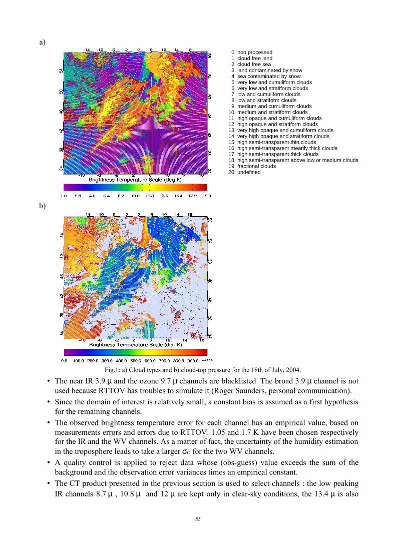
a)

0 non processed 1 cloud free land 2 cloud free sea 3 land contaminated by snow 4 sea contaminated by snow 5 very low and cumuliform clouds 6 very low and stratiform clouds 7 low and cumuliform clouds 8 low and stratiform clouds 9 medium and cumuliform clouds10 medium and stratiform clouds11 high opaque and cumuliform clouds12 high opaque and stratiform clouds13 very high opaque and cumuliform clouds14 very high opaque and stratiform clouds15 high semi-transparent thin clouds16 high semi-transparent meanly thick clouds17 high semi-transparent thick clouds18 high semi-transparent above low or medium clouds19 fractional clouds20 undefined

b)

Fig.1: a) Cloud types and b) cloud-top pressure for the 18th of July, 2004.

• The near IR 3.9 µ and the ozone 9.7 µ channels are blacklisted. The broad 3.9 µ channel is notused because RTTOV has troubles to simulate it (Roger Saunders, personal communication).

• Since the domain of interest is relatively small, a constant bias is assumed as a first hypothesisfor the remaining channels.

• The observed brightness temperature error for each channel has an empirical value, based onmeasurements errors and errors due to RTTOV. 1.05 and 1.7 K have been chosen respectivelyfor the IR and the WV channels. As a matter of fact, the uncertainty of the humidity estimationin the troposphere leads to take a larger σO for the two WV channels.

• A quality control is applied to reject data whose (obs-guess) value exceeds the sum of thebackground and the observation error variances times an empirical constant.

• The CT product presented in the previous section is used to select channels : the low peakingIR channels 8.7 µ , 10.8 µ and 12 µ are kept only in clear-sky conditions, the 13.4 µ is also

85

kept above very low clouds and the two WV channels are considered even above mid-levelclouds.

4.2.4. Impact on analysesA test period of 15 days with 4 daily assimilations has been performed from the 6th to the

22nd of July, 2004. In order to study the relative impact of SEVIRI data within ALADIN 3D-Var, acontrol experiment (CNTRL hereafter) has been run. This experiment follows the configurationpresented by Fischer et al. (2004) : an Ensemble B matrix (Stefanescu and Berre, 2004) has beenused with an a-posteriori tuning of the REDNMC factor, to 1.8. It assimilates the same complete setof observations as ARPEGE at that time (AMSU-B microwave radiances and the sea-windscatterometer on board QuikSCAT are in particular not taken into account in these experiments),within an assimilation window of +/- 3 hours. 36 h forecast have been run from each analysis timewith digital filter initialization applied.

An experiment that presents the same characteristics than CNTRL but with the addition ofSEVIRI radiances (SEV hereafter) has then been run during the same period. Assimilation statisticsplotted in Fig. 2 show that a lot of information coming from the 6 assimilated channels is taken intoaccount in the analyses. The (obs-analysis) root-mean-square (RMS) errors over the whole testperiod are indeed much lower than the (obs-guess) ones. The relative error decrease is however lesspronounced for the 13.4 µ channel as noted in Montmerle (2004) which is probably due to thebroader shape of its weighting function and/or the choice of a non-optimal observation errorvariance. The mean biases have values less than 0.2 K which seems to justify the values of theconstant bias correction.

Monitoring has been performed and results are plotted on Fig. 3 for the six assimilatedchannels. It shows firstly a strong negative bias of about –2.6 K for the WV 6.2 µ channel, which iswell corrected by the flat bias correction. As for the 3.9 µ channel which is blacklisted, this bias isdue to its broad spectral resolution that is badly taken into account by the radiative transfert modelRTTOV. The bias-corrected channels present very stable features during the period. A diurnal cycleis visible for the biases and the number of active data for the low peaking channels. For eachanalysis time, about 1500 observations from the WV channels, 1000 for the 13.4 µ one and between500 and 1000 for the three other channels are considered in the variational process. The (obs-guess)RMS error presents also a weak oscillation for the WV 6.2 µ that coincides with two peaks ofconvective activity at the beginning and at the end of the test period.

Fig.2: Assimilation statistics of the SEV experiment computed considering every analysis times over the July 2004 testperiod. The vertical axis denotes the channel number, the left panel the RMS error and the right panel the bias between(obs – guess) (plain line) and (obs-analysis) (dashed line) for brightness temperature. The number of assimilated data isplotted between two panels.

86

Fig.3: Monitoring for the 6 assimilated SEVIRI channels for the SEV experiment from the 6th to the 18th of July, 2004.Histograms on bottom of figures (associated with the right vertical axis) represent the number of active data that enterthe minimization.

87

4.2.5. Impact on forecast✗ Forecast scores

DA.r12/TP – SEV.r12/TP(15 cases, 06/07/2004 12UTC -> 22/07/2004 12UTC)

Std Dev RMS BIAS

Geopotential(1 m)

T(0.05 K)

q(1 %)

Wind(0.2 m/s)

Fig.4: Differences in forecast scores against TEMP observations : DA vs SEV, over the ALADIN-France domain for theJuly 2004 test period. Left column is the standard deviation, middle the RMS error and right the bias. Green isolinesdenote positive impact of SEV.

88

Forecast scores have been computed relatively to the dynamical adaptation version ofALADIN (DA) and are plotted in Fig. 4. For the geopotential height, the assimilation of SEVIRIdata reduces the bias against radiosoundings of about 4 m between 12 and 24 h of forecast above600 hPa, and increases it slightly below. This impact induces logically negative bias on sea-levelpressure during the forecast, which is difficult to explain since no negative bias is present in theanalyses. For the temperature, SEV brings a diminution of RMS error on all vertical levels before12 h and up to 24 h near 300 hPa. Negative bias are however present from the start above 300 hPaand in the middle troposphere after 6 h. The RMS error for humidity is slightly improved before 6 hof forecast and up to 12 h near 400 hPa. The analyses for this quantity show however small biases atall vertical levels that propagate downward with time. Finally, SEV show better scores than CNTRLon RMS error of the wind intensity in mid- to-high troposphere (CNTRL scores are not shown).

Globally, the scores of CNTRL against radiosoundings have been slightly degraded. This canbe explained by the fact that the large amount of SEVIRI data added in the assimilation process hasslightly taken away the analysis from radiosoundings observations which are the main source ofobservation in CNTRL. To give better weight to the different observation types, the tuning of theobservation error variances will be undertaken in the near future, following Chapnik (2004).

✗ Total rainfall forecastCase of the 18 th July 2004 The total rain forecasted between 6 and 12 hours by DA, CNTRL and the SEV experiments

from the 00 UTC analysis time are plotted on Fig. 5 and compared to rain-gauge values over France.DA missed the NE/SW orientation of the main rain band. CNTRL produces the good orientationand the SW part of the line seems realistic, although a little bit too South. The use of SEVIRI dataallows to forecast the observed second cell of intense precipitations located in the NE part of theline, with a slightly overestimated amount (> 20 mm). The maximum over the Bordeaux region ishowever located too South but with an amount of 40 mm comparable to rain-gauge observations.The secondary line of precipitation is also quite well captured over the NE of France with realisticshape and amount.

To understand why SEV produces the observed second cell of intense precipitations in thenorth-eastern part of the line contrary to CNTRL, increments of humidity and temperature at700 hPa for the 00 UTC analysis have been plotted for the two experiments (Fig. 6). The moststriking difference between the two is that increments produced by SEV present more realistic andmesoscale patterns than for CNTRL, where the main source of information seems to come mainlyfrom radiosoundings. In particular, SEVIRI data are cooling and humidifying the mid-to-lowtroposphere pre-convective area located upstream of the frontal rain band over western France,which produces intense rain 6 hours later.

At each analysis time, a large amount of IR radiances coming from SEVIRI is taken intoaccount in the assimilation process compare to ATOVS data for example. The ratio of the numberof data that enters the screening for these two observation types is varying indeed between 10 and25. It has however to be noted that for both CNTRL and SEV, ATOVS data have been assimilatedusing the screening features of ARPEGE. For HIRS for instance, 1 pixel out of 5 have beenextracted and thinning boxes of 250 km2 have been applied which is not comparable to SEVIRI. Inthe near future, the impact of a higher density of ATOVS data will be tested in 3D-Var using twocomplementary approaches :

• Extraction and thinning at higher horizontal resolutions, • Use of the "EARS-Lannion" data that are already used in the operational ARPEGE suite. Their

shorter reception time delay allows indeed to get more data within the +/- 3 hours assimilationwindow considered in ALADIN 3D-Var.

89

DA

CNTRL

OBS

SEV

Fig.5: Rain-gauge observation (top right) and simulated total rainfall between 6-12 h of forecast for July 18th, 2004.

q increments at 700 hPa

T increments at 700 hPa

CNTRL SEV

Fig.6: Specific humidity (top panels) and temperature increments (bottom panels) for CNTRL (left) and SEV (right), for July 18th, 2004, at 00 UTC.

90

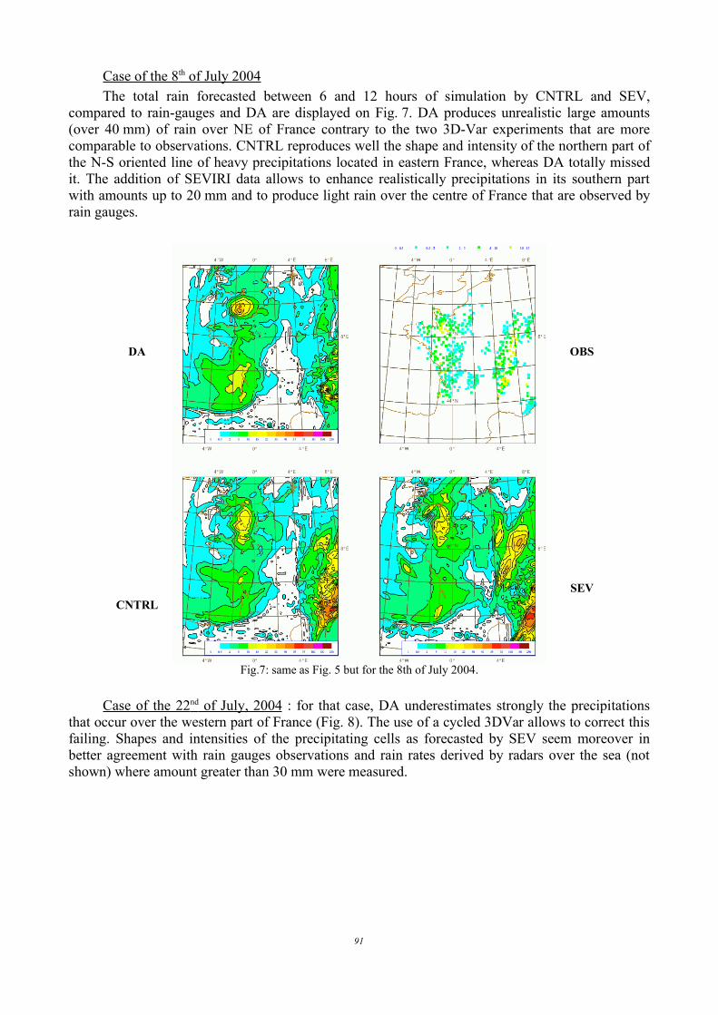
Case of the 8 th of July 2004 The total rain forecasted between 6 and 12 hours of simulation by CNTRL and SEV,

compared to rain-gauges and DA are displayed on Fig. 7. DA produces unrealistic large amounts(over 40 mm) of rain over NE of France contrary to the two 3D-Var experiments that are morecomparable to observations. CNTRL reproduces well the shape and intensity of the northern part ofthe N-S oriented line of heavy precipitations located in eastern France, whereas DA totally missedit. The addition of SEVIRI data allows to enhance realistically precipitations in its southern partwith amounts up to 20 mm and to produce light rain over the centre of France that are observed byrain gauges.

DA

CNTRL

OBS

SEV

Fig.7: same as Fig. 5 but for the 8th of July 2004.

Case of the 22 nd of July, 2004 : for that case, DA underestimates strongly the precipitationsthat occur over the western part of France (Fig. 8). The use of a cycled 3DVar allows to correct thisfailing. Shapes and intensities of the precipitating cells as forecasted by SEV seem moreover inbetter agreement with rain gauges observations and rain rates derived by radars over the sea (notshown) where amount greater than 30 mm were measured.

91

DA

CNTRL

OBS

SEV

Fig.8: same as Fig. 5 but for the 22nd of July 2004

✗ QPF scoresQuantitative Precipitation Forecast (QPF) scores were computed for the July test period for

different thresholds. The observations used to compute those scores are the 6 hours total rainmeasured by rain gauges.

Fig.9: QPF scores for DA, CNTRL and SEV computed for the whole July period for the total rain forecasted between12 and 6 h, from the 00 and the 12 UTC analyses. Precipitation thresholds are 0.1, 1, 2, 5, 10 and 30 mm.FBIAS : Frequency Bias, POD : Probability Of Detection, ETS : Equitable Threat Score, FAR : False Alarme Rate

The two detection scores (ETS and POD) displayed in Fig. 9 are higher for the experiments

92

that are using an assimilation scheme. The ETS is comparable for CNTRL and SEV and showsvalues almost twice greater than DA for the 5 mm threshold. The addition of SEVIRI data permitsto perform a better detection of precipitating events mostly for the 2 and the 5 mm thresholds, withrespective POD of 0.46 and 0.23 compared to 0.34 and 0.16 with CNTRL. However, this betterdetection is made to the detriment of the FBIAS : SEV produces to much precipitations for allthresholds. For small thresholds, the overestimation of the number of simulated precipitating pixelsshown by DA and CNTRL is accentuated for SEV. For thresholds greater than 5 mm, the FBIAS arecomparable for the 3 experiments although slightly greater than 1 for SEV. Finally, the FAR isgreater for SEV for the 30 mm threshold. Since a very small number of observed/simulated pixelsare characterized by values greater than this threshold, QPF scores are weakly representative at thislevel.

Assimilating SEVIRI data using the first configuration defined in this report seems thus toproduce too much precipitation, particularly light rain. The weight of the information given by theseradiances during the assimilation step has to be weaken to limit this drawback through the tuning ofthe observation error variances and/or the use of larger thinning boxes. 4.2.6. Conclusions and future work

SEVIRI data have then been assimilated in ALADIN 3D-Var following the configurationdefined by Fischer et al. (2004) to study their relative impact. Channels 3.9 µ and 9.7 µ have beenblacklisted, 1 pixel out of 5 has been used, a constant bias has been applied for each channel andempirical error variances have been chosen in the first configuration. The cloud-type classificationcomputed by CMS in the SAF/NWC framework has been used to keep data non contaminated byclouds in the variational process, which includes channels that peak over the cloud top. Themonitoring shows stable features for all channels during the whole test period. A lot of informationcoming from SEVIRI radiances is taken into account in the analyses through the 3D-Var, producingrealistic increments. Results deduced from the 15 days test period are encouraging notably for theshort term (i.e < 12 h) precipitation forecasts, where the addition of these kind of data allows tosimulate realistic precipitation patterns, in shape and intensity. Forecast scores are slightly degradedcompared to the control experiment, probably because of the large amount of additional data thatmove slightly away the analyses from radiosoundings. Moreover, QPF scores have shown that theexperiment that includes SEVIRI radiances has better rain detection scores but produces spatiallytoo much light precipitations.

One priority in the near future will thus be to tune error statistics and/or thinning to lower therelative impact of SEVIRI in the analyses. Methods based on the use of the DFS (Degrees ofFreedom for Signal) related quantities will be applied to improve covariances matrices (Desroziersand Ivanov, 2001; Chapnik, 2004). In parallel, studies will be addressed to the use of additionalATOVS data by considering radiances coming from EARS extracted with a better sampling. Inparticular, the impact of AMSU-B data is one major concern. Finally, the cloud-top pressureproduct sent by CMS and a convection-detection algorithm will be used to compute proxy humidityprofiles for convective clouds for assimilation purposes.

The first configuration of ALADIN 3D-Var (including SEVIRI radiances) is scheduled tobecome operational hopefully around March 2005. Further tests are envisaged on this operationalsuite, including the use of a 3D-Var FGAT (First Guess at Appropriate Time) and shorterassimilation cycles (typically 3 hours). 4.2.7. References:Chapnik, B., G. Desroziers, F. Rabier, and O. Talagrand. 2004. Diagnosis and tuning of observational errorstatistics in a quasi operational data assimilation setting. Q. J. R. Meteo. Soc., Accepted for publication.Desroziers, G. and S. Ivanov, 2001: Diagnosis and adaptative tuning of observation error parameters in avariational assimilation. Q. J. R. Meteo. Soc., 127, 1433-1452.Fischer, C., T. Montmerle and L. Berre, 2004: Evaluation of a limited area data assimilation cycle at Meteo-France. SRNWP/Met Office/HIRLAM Workshop, Exeter, UK, 15-17 nov.

93

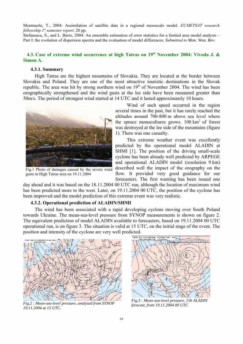
Montmerle, T., 2004: Assimilation of satellite data in a regional mesoscale model. EUMETSAT researchfellowship 1st semester report. 20 pp.Stefanescu, S., and L. Berre, 2004: An ensemble estimation of error statistics for a limited area model analysis –Part I: the evolution of dispersion spectra and the evaluation of model differences. Submitted to Mon. Wea. Rev.

4.3. Case of extreme wind occurrence at high Tatras on 19th November 2004: Vivoda J. &Simon A.

4.3.1. Summary High Tatras are the highest mountains of Slovakia. They are located at the border between

Slovakia and Poland. They are one of the most attractive touristic destinations in the Slovakrepublic. The area was hit by strong northern wind on 19th of November 2004. The wind has beenorographically strengthened and the wind gusts at the lee side have been measured greater than50m/s. The period of strongest wind started at 14 UTC and it lasted approximately 10 hours.

Wind of such speed occurred in the regionseveral times in the past, but it has rarely reached thealtitudes around 700-800 m above sea level wherethe spruce monocultures grows. 100 km2 of forestwas destroyed at the lee side of the mountains (figure1). There was one casualty.

This extreme weather event was excellentlypredicted by the operational model ALADIN atSHMI [1]. The position of the driving small-scalecyclone has been already well predicted by ARPEGEand operational ALADIN model (resolution 9 km)described well the impact of the orography on theflow. It provided very good guidance for ourforecasters. The first warning has been issued one

day ahead and it was based on the 18.11.2004 00 UTC run, although the location of maximum windhas been predicted more to the west. Later, on 19.11.2004 00 UTC, the position of the cyclone hasbeen improved and the model prediction of this extreme event was very realistic. 4.3.2. Operational prediction of ALADIN/SHMI

The wind has been associated with a rapid developing cyclone moving over South Polandtowards Ukraine. The mean-sea-level pressure from SYNOP measurements is shown on figure 2.The equivalent prediction of model ALADIN available to forecasters, based on 19.11.2004 00 UTCoperational run, is on figure 3. The situation is valid at 15 UTC, on the initial stage of the event. Theposition and intensity of the cyclone are very well predicted.

94

Fig.2 : Mean-sea-level pressure, analysed from SYNOP 19.11.2004 at 15 UTC.

Fig.3 : Mean-sea-level pressure, 15h ALADIN forecast, from 19.11.2004 00 UTC

Fig.1 Photo of damages caused by the severe windgusts in High Tatras area on 19.11.2004

As the cyclone was moving, the wind direction changed from western to northern wind.During the period of the strongest wind, the flow was almost perpendicular to the mountain ridge.The model has simulated an effect similar to hydraulic jump (more in the next section) and thedownslope windstorm has been formed at the lee side with strong turbulence. The maximum windgusts in the operational prediction exceeded 40 m/s while average wind was around 20 m/s.

The prediction of wind gusts is shown in figures 4 and 5. It is the +16h and +17h operationalmodel forecasts from 19.11.2004 00 UTC. The green color represents the wind gusts above 25 m/s,the yellow color above 30 m/s and the red color above 40 m/s.

4.3.3. High resolution prediction of ALADIN

The operational prediction was not detailed enough to capture exactly the areas where theforest has been destroyed. To further improve model prediction of wind we ran the ALADIN modelwith a 2.5 km resolution in order to describe orography more realistically. The model was integratedhydrostatically with the same model settings as the operational model except that convection wasturned off, horizontal diffusion was adjusted to the new resolution and the model time-step was100 s.

Fig.6: The direction of vertical cross section on figure 7.

95

Fig.4: Instantaneous wind gust +17h prediction fromALADIN/SHMI operational run from 19.11.200400UTC

Fig.5:Instantaneous wind gust +16h prediction fromALADIN/SHMI operational run from 19.11.200400UTC

Fig.7: Vertical cross-section perpendicular to High Tatrasand Low Tatras ridges. Hydraulic jump is visible in the fieldof potential temperature (coloured isolines). The windspeed (white contours) is locally strengthened in the area ofjump. From high resolution experimental run, 19.11.200400 UTC +16h.

The effect of hydraulic jump was very apparent in the high-resolution run. It is clearly visiblein the potential-temperature field on figure 7. If we consider almost adiabatic processes, then the airparticles follow the potential-temperature isolines, descending very deep along the lee side of themountains and successively after on ascending very quickly to its original altitude. This forms theshallow high velocity, very turbulent flow at the lee side near the surface, because streamlinesdensity is very high in this region. Another but less intensive jump has been predicted behind LowTatras ridge. The direction of the vertical cross section is shown on figure 6.

The area with the strongest wind gusts coincides with the area of observed wind breakages atthe lee side of High Tatras. The wind gusts from the high-resolution run are shown on figure 8 forthe 16 h forecast range, when the strongest wind gusts were predicted. The maximum values ofgusts are greater than 50 m/s. The area of observed forest damages, provided by Slovakenvironmental agency, is depicted by red color on figure 9. Although the density of the observingstations is not sufficient to verify all the features predicted by ALADIN, we assume that theprediction was very precise, because the area of maximum wind gusts is almost identical to the areawith observed breakage.

The second maximum of wind gusts was predicted to the South of High Tatras (figure 8). It isthe area of Low Tatras mountain, where wind gusts above 50 m/s were really observed. However,we do not have available the map with damages in this area.

4.3.4. ReferencesDerková, Belluš, Mašek, Španiel and Vivoda : New Operational ALADIN setup at SHMI, ALADIN Newsletter27, 2005

4.4. High-resolution dynamical adaptation of the wind forecast using the non-hydrostaticversion of the ALADIN model: Alexandru S.

ABSTRACTThe high-resolution dynamical adaptation procedure of the wind field from the low-troposphere consists in the interpolation

of the wind forecast of the ALADIN model to a higher resolution, taking into account the new description of the surface parameters(as a result of increasing the resolution). It is well known that the surface wind is highly influenced by the orography described into aNWP model. By increasing the resolution, the orography has been improved, and consequently the surface wind field is expected tobe a better forecast. Two case studies have been investigated for some meteorological situations. The novelty of these experiments isthat the non-hydrostatic version of the ALADIN model has been used. PHYSICAL PROCESSES

4.4.1. IntroductionThe wind field from the planetary boundary layer is influenced by the orography described in

the model. There are many situations when the surface wind is mis-forecasted, mainly in the

96

Fig. 8: Instantaneous wind gust +16h prediction fromALADIN high resolution (2.5km) run from 19.11.200400UTC. Zoom over High Tatras.The frame selects thearea showed on figure 9.

Fig.9: The High Tatras with the area of destroyed forest(red color). Courtesy of Slovak EnvironmentalProtection Agency (http://www.sopsr.sk)

mountainous regions or on the seaside, because the orography in the model is smoother than inreality. So it happens that some points over the mountains are at a lower altitude or, on the seaside,some grid-points, which are located on land, are considered as being on water.

The dynamical adaptation procedure of the surface wind at high resolution has been developedby Zagar and Rakovec (1999) and is performed in two steps. First the wind forecast of theALADIN/Romania hydrostatic model at 10 km horizontal resolution is interpolated to a finer grid ofabout 2.5 km. As a result of increasing the resolution, the representation of the surface parameters(including the orography) has been improved (comparing with those of the coupling model). Thusthe wind field is influenced by the new model orography. After the interpolation to the highresolution, the next step of the dynamical adaptation of the wind field to these new characteristics ofthe orography is the integration of the non-hydrostatic model, for a corresponding period of time(for 30 minutes with a time-step of 60 seconds). Because the time-scale for some physical processesis longer than the necessary time for the dynamic adjustment of the fields, parts of the physicalparameterizations are further omitted. As mentioned by Zagar and Rakovec, if the coupling modelfails to have a reasonable prediction in some special meteorological situations, the dynamicaladaptation of the wind field at higher resolution cannot improve the forecast.

Because the wind forecast is mainly influenced by the orography, the number of vertical levelsdescribing the higher troposphere and stratosphere has been reduced. Thus from the 41 levels in theoperational version of the ALADIN/Romania model, only 26 levels have been kept. These aremainly located in the lower part of the troposphere (Figure 1).

Fig.1: Distribution of the vertical levels for the ALADIN/Romania model in dynamical adaptation at high resolution(left side) and for the operational one (right side)

4.4.2. The experimental resultsThe experiments have been performed for two cases : for the 12th - 13th of October 2004 and

for the 17th - 18th of October 2004. They were selected because the 10 m wind intensity reachedvalues of about 25 m/s in the mountainous region. The hydrostatic model has been integrated at10 km horizontal resolution, in order to have a reference for the experiments at high resolution. Thedynamical adaptation of the surface wind was carried out on a domain covering Romania at 2.5 kmresolution.

The results of the reference experiment can be seen in Figure 2, where the forecast of thesurface wind field of ALADIN/Romania at 10 km resolution is represented for the case from the 17th

97

of October 2004. In order to point out the region of interest, the pictures represent a zoom confinedwithin 45°- 47.5°N in latitude and 23°- 27°E in longitude.

Fig. 2: The 12h forecast of 10 m wind field, performed by the ALADIN/Romania hydrostatic model at 10 km, from17.10.2004 00 UTC run, together with the real measurements of the wind (represented by red barbs)

In Figure 3 the forecasts of the wind field from the low troposphere with theALADIN/Romania model in its non-hydrostatic (left side) and hydrostatic (right side) versions at2.5 km horizontal resolution are compared. As one can see the differences between the results of themodel appeared mainly in the regions of high orography. Having a better representation of theorography, new valleys and higher peaks appeared. These new features influence mainly the winddirection. Regarding the forecast of the wind intensity, both versions of the model at 2.5 kmresolution succeeded to give a rather good prediction, although the biggest values of the 10 m wind,as measured in the Meridional Carpathian Mountains (in the southern part of Figure 3), were notforecasted.

Fig.3: The 10 m wind forecast in dynamic adaptation at 2.5 km resolution, performed by the non-hydrostatic (left side),and the hydrostatic (right side) ALADIN/Romania model from 17.10.2004 00 UTC run, valid at 13 UTC, together with

the real measurements of the wind (represented by red barbs)

Another method to evaluate the results of the dynamical adaptation procedure of surface windat high resolution consists in computing some statistical measures (such as standard deviation ormean absolute error). Figure 4 presents the standard deviation scores of all three experiments. One

98

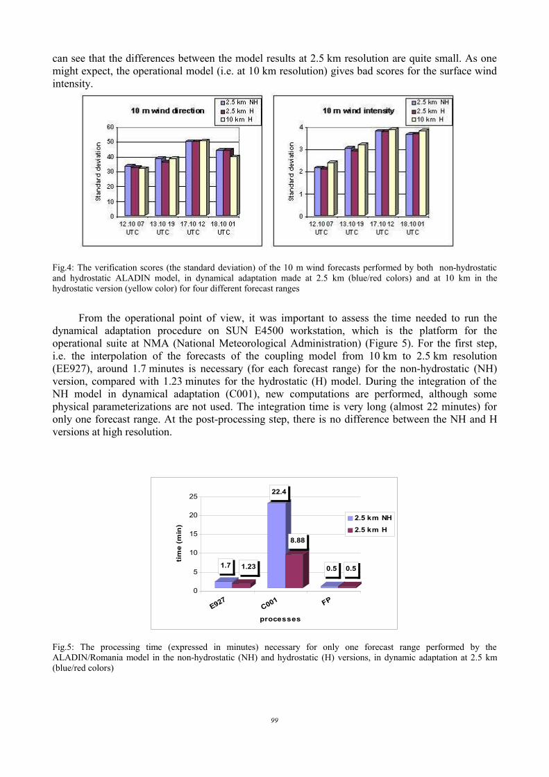
can see that the differences between the model results at 2.5 km resolution are quite small. As onemight expect, the operational model (i.e. at 10 km resolution) gives bad scores for the surface windintensity.

Fig.4: The verification scores (the standard deviation) of the 10 m wind forecasts performed by both non-hydrostaticand hydrostatic ALADIN model, in dynamical adaptation made at 2.5 km (blue/red colors) and at 10 km in thehydrostatic version (yellow color) for four different forecast ranges

From the operational point of view, it was important to assess the time needed to run thedynamical adaptation procedure on SUN E4500 workstation, which is the platform for theoperational suite at NMA (National Meteorological Administration) (Figure 5). For the first step,i.e. the interpolation of the forecasts of the coupling model from 10 km to 2.5 km resolution(EE927), around 1.7 minutes is necessary (for each forecast range) for the non-hydrostatic (NH)version, compared with 1.23 minutes for the hydrostatic (H) model. During the integration of theNH model in dynamical adaptation (C001), new computations are performed, although somephysical parameterizations are not used. The integration time is very long (almost 22 minutes) foronly one forecast range. At the post-processing step, there is no difference between the NH and Hversions at high resolution.

Fig.5: The processing time (expressed in minutes) necessary for only one forecast range performed by theALADIN/Romania model in the non-hydrostatic (NH) and hydrostatic (H) versions, in dynamic adaptation at 2.5 km(blue/red colors)

99

1.7 1.23

22.4

8.88

0.5 0.5

0

5

10

15

20

25

tim

e (m

in)

E927C001 FP

processes

2.5 km NH2.5 km H

4.4.3. ConclusionsIn this paper, the preliminary results of the procedure for the dynamical adaptation of the

surface wind forecast of the ALADIN/Romania using the non-hydrostatic version are presentedbriefly. For the two selected cases, the results of the NH and H models are relatively similar. Inaddition, taking into account the processing time (almost three times longer for the ALADIN/NHthan for the ALADIN/H model), we consider that the experiments performed were not convincingenough to state the necessity of using the non-hydrostatic model for the dynamical adaptationprocedure of the wind field. In this respect more investigations are needed.

4.4.4. ReferencesZagar, M., and Rakovec, J., 1999: Small-scale surface wind prediction using dynamic adaptation. Tellus, 51, 489– 504.

4.5. Pre-operational testing of a 3D-VAR assimilation in ALADIN-FRANCE: Fischer C., Th.Montmerle & L. Berre.

ABSTRACTWe explain the aim, strategy and first results for the implementation of an operational variational data assimilation system in

the ALADIN-France model. Starting from the experiences gathered over the last five years with 3D-VAR in ALADIN as a researchconfiguration, the goal is to settle a continuous, permanent assimilation cycle with an initial update frequency of 6 hours. ARPEGEdata plus extra data (Meteosat-8 radiances to start with) are considered. The goal is to obtain at least as good conventional scoresover Western Europe as with ARPEGE, plus a beneficial effect on short-range wind, temperature and precipitation forecasts. Theretained solution offers such an improvement, with better precipitation "scores" at least up to 12 hours. In 2005, this assimilationcycle will be improved by more frequent updates and additional algorithmic facilities.

4.5.1. Initial choicesThe core choices are the following, starting from earlier experiences gathered in the four

leading ALADIN centres (Budapest, Casablanca, Prague, Toulouse) :• analysis every 6 hours, in a continuous cycle, to mimic the ARPEGE system, • lagged Jb formulation with a specific error variance inflation (after the works by M. Široka, W.

Sadiki), • ARPEGE observations to ensure a maximum of variety and coverage of observations acting as

the main constraint in the problem, at our present knowledge (and technical ability), • accompanying developments : Olive configuration, interaction with the AROME project and the

GMME group, • evaluation using a mixture of conventional COMPAS-type scores (for synoptic and meso-alpha

scales) and subjective evaluation on chosen situations for meso-beta and large convective scales

4.5.2. Impact of B matrix and statistical behaviour of the assimilation

The first striking results from a one-month cycle were very bad scores on temperature, biaserrors in the stratosphere and at tropopause level. Investigations have shown that this bias is due to amodel error, present both in ARPEGE and ALADIN, though we have not been able to pinpoint theactual cause (dynamics or physics for instance). This negative behaviour, in the analysis itself (theanalysis being even worse than the initial state of dynamical adaptation), had a detrimental impacton 6 hour forecasts and background scores, throughout most of the troposphere and for all fields.The cure was to change both the B matrix (sampling) and the global tuning of error variances(REDNMC). Thanks to S. Stefanescu's investigations on an ensemble-derived B sampling, we haveswitched to the ensemble Jb which does have statistical characteristics intermediate between the

100

lagged and standard NMC ones. For instance, correlation length-scales are shorter than in theclassical NMC case, which is suitable for keeping mesoscale analysis increments, but larger than inthe lagged case, which allows to spread the observation information content into data-poor areaswhere the background may be of low quality. Additionally, the error variances are significantlyinflated (by a factor of 1.82 ). Figure 1 shows the scores for background and analysis, forexperiments using the lagged (red) and ensemble (black) Jb formulations, in the space of radiosondetemperature observations. The improvement of the analysis is striking, for the ensemble case..

Fig.1: RMS and bias computed for radiosonde temperatures. Lagged Jb (red), ensemble Jb (black)

4.5.3. Case studies✗ 20/07/04

This is a case with a synoptic-scale front passing over France and Germany at the time ofinterest. The front exhibits interesting mesoscale features, such as a maximum over the Mosel valleyin Germany (unfortunately no rain-gauge coverage is available for this area, Figure 2), small-scalemaxima over the Western edges of the Massif Central and the Dordogne area. The operationalALADIN-France dynamical adaptation over-exaggerated the Mosel valley event, and produced awide shed of rain over South-Western France (Figure 3), where mostly dry conditions wereobserved. The data assimilation cycles produce more realistic amounts of precipitations overGermany and the Massif Central. With a lagged Jb, the front has a very narrow and strong structure,which is not the case with the ensemble Jb. This latter, wider structure, probably is closer to thetruth. The data assimilation cycles generally produce no or little precipitation over South-WesternFrance.

101

Fig.2: raingauge measurements

Fig.3: 12h-6h cumulated precipitations. Lagged Jb (top left), ensemble Jb + DFI (top right), ensemble Jb – no DFI(bottom left), dynamical adaptation (bottom right)

102

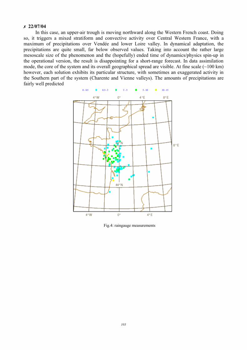
✗ 22/07/04In this case, an upper-air trough is moving northward along the Western French coast. Doing

so, it triggers a mixed stratiform and convective activity over Central Western France, with amaximum of precipitations over Vendée and lower Loire valley. In dynamical adaptation, theprecipitations are quite small, far below observed values. Taking into account the rather largemesoscale size of the phenomenon and the (hopefully) ended time of dynamics/physics spin-up inthe operational version, the result is disappointing for a short-range forecast. In data assimilationmode, the core of the system and its overall geographical spread are visible. At fine scale (~100 km)however, each solution exhibits its particular structure, with sometimes an exaggerated activity inthe Southern part of the system (Charente and Vienne valleys). The amounts of precipitations arefairly well predicted

Fig.4: raingauge measurements

103

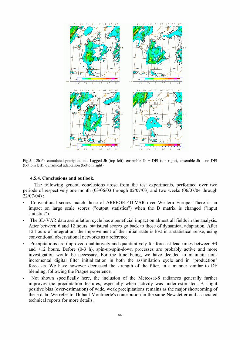
Fig.5: 12h-6h cumulated precipitations. Lagged Jb (top left), ensemble Jb + DFI (top right), ensemble Jb – no DFI(bottom left), dynamical adaptation (bottom right)

4.5.4. Conclusions and outlook.The following general conclusions arose from the test experiments, performed over two

periods of respectively one month (03/06/03 through 02/07/03) and two weeks (06/07/04 through22/07/04) :• Conventional scores match those of ARPEGE 4D-VAR over Western Europe. There is an

impact on large scale scores ("output statistics") when the B matrix is changed ("inputstatistics").

• The 3D-VAR data assimilation cycle has a beneficial impact on almost all fields in the analysis.After between 6 and 12 hours, statistical scores go back to those of dynamical adaptation. After12 hours of integration, the improvement of the initial state is lost in a statistical sense, usingconventional observational networks as a reference.

• Precipitations are improved qualitatively and quantitatively for forecast lead-times between +3and +12 hours. Before (0-3 h), spin-up/spin-down processes are probably active and moreinvestigation would be necessary. For the time being, we have decided to maintain non-incremental digital filter initialization in both the assimilation cycle and in "production"forecasts. We have however decreased the strength of the filter, in a manner similar to DFblending, following the Prague experience.

• Not shown specifically here, the inclusion of the Meteosat-8 radiances generally furtherimproves the precipitation features, especially when activity was under-estimated. A slightpositive bias (over-estimation) of wide, weak precipitations remains as the major shortcoming ofthese data. We refer to Thibaut Montmerle's contribution in the same Newsletter and associatedtechnical reports for more details.

104

• An E-suite is planned for about February 2005, based on CY29T1. Meteosat-8 radiances will beincluded.

4.5.5. BibliographyMontmerle, T.: Use of geostationnary SEVIRI radiances in ALADIN 3DVAR, ALADIN Newsletter 27, 2005Sadiki, W. and Fischer, C.: A posteriori validation applied to the 3D-VAR ARPEGE and ALADIN dataassimilation systems, Tellus, 57A, pp. 21-34, 2005Široka, M., Fischer, C., Cassé, V., Brozkova, R. and Geleyn, J.-F.: The definition of mesoscale selective forecasterror covariances for a limited area variational analysis, Meteor. Atmos. Ph., 82, pp. 227-244, 2003Stefanescu, S.E., Berre, L. and Belo Pereira, M.: An ensemble estimation of error statistics for a limited areamodel analysis. Part I: The evolution of dispersion spectra and the evaluation of model differences, 2005, inpreparationBerre, L., Stefanescu, S.E. and Belo Pereira, M.: An ensemble estimation of error statistics for a limited areamodel analysis. Part II: A formal and experimental comparison with two other error simulation methods, 2005, inpreparation

4.6. Latest results of the LAMEPS experiments: Hágel E.ABSTRACTIn this paper we are presenting the main results of a two months stay in Toulouse (October-November, 2004). The research

carried out during this two months was a continuation of the work started at HMS in the topic of short range ensemble forecasts.(The full length report of this stay is available on the ALADIN webpage: http://www.cnrm.meteo.fr/aladin/publications/report.html.)

4.6.1. MotivationThe ensemble technique is based on the fact that small errors in the initial condition of any

numerical weather prediction model (or errors in the model itself) can cause big errors in theforecast. When making an ensemble forecast the model is integrated not only once (starting from theoriginal initial condition), but forecasts are also made using little bit different (perturbed) initialconditions. This ensemble of the initial conditions consists of equally likely analyses of theatmospheric initial state and, in an ideal case, encompasses the unknown 'true' state of theatmosphere. This technique is capable to predict rare or extreme events and has the advantage ofpredicting also the probability of future weather events or conditions. Despite its success, at themoment the ensemble method is mainly used for medium range forecasting and on global scales,but nowadays the emphasis is more and more moving towards the short ranges and smaller scales.However, methods used in the medium range can not be directly applied to short range forecasting.Research has already been done in this field and there are some operational or quasi-oparationalshort range ensemble systems (e.g. at Météo-France, at NCEP, the COSMO-LEPS, or the SRNWP-PEPS project at DWD). We also wish to develop a short range ensemble system for the CentralEuropean area, with the main goal being the better understanding and prediction of local extremeevents like heavy precipitation, wind storms, big temperature-anomalies and also to have a highresolution probabilistic forecast for 2 meter temperature, 10 meter wind and precipitation in the 12-48h time range.

4.6.2. ExperimentsFor making an ensemble forecast lots of methods can be used (e.g. multi-model, multi-

analysis, perturbation of observations, singular vector method, breeding etc.). It is not known yet(especially at mesoscale) which method would provide the best forecasts. It was decided to start ourexperiments with the downscaling of the global (ARPEGE based) ensemble. This work can bedivided into two parts:

Direct downscaling of the ARPEGE/PEACE3 members3 Prévision d'Ensemble A Courte Echéance; a short-range ensemble system operational at Météo-France, with 10+1 members, based on the model

ARPEGE

105

Investigation of the impact of target domain and target time window in the computation ofsingular vectors and downscaling the ARPEGE ensemble members

From previous studies (see Hágel and Szépszó, 2004) performed at the HungarianMeteorological Service (HMS), we found that by simply downscaling the PEACE members thespread obtained is not big enough in the area of our interest (Central Europe). This fact can beexplained easily if we consider that the PEACE system was calibrated in order to get enough spreadover Western Europe between 24 and 72 h steps, for wind speed, 500 hPa geopotential and meansea level pressure. The aim of the PEACE system is to detect strong storms. This raises somequestions:

Are the PEACE provided initial and boundary conditions convenient for the local EPS run, fora Central European application?What is the impact of different target domains and target times in the singular vectorcomputation?During this two month stay - as a continuation of the work started at HMS - we tried to

investigate and better understand the impact of different target domains and target times in thesingular vector computation. In our experiments an ARPEGE ensemble system was used, based onan earlier version of the PEACE system:

For the generation of perturbations the singular vector method was usedThe singular vector computations were performed on T63 resolution10 ensemble members were computed + the control runThe integrations were performed on T199 resolutionThe forecast length was 54h (we use 54h because of the verification of precipitation, since thedaily precipitation amount is observed at 06 UTC, so a 48h forecast started from the 00 UTCanalysis would only cover one 24h period like this, while a 54h forecast covers both)

The main difference between the PEACE system and the system used by us is that the targetdomain and the target time was not fixed. For the target time 12h and 24h were used, and differenttarget domains were defined.

In previous studies performed at the Hungarian Meteorological Service, we tried to investigatethe effect of different target domains. Four domains were defined (fig. 1):

Domain 1: Atlantic Ocean and Western Europe (70N/260W/30S/20E; the same as used earlierin PEACE)Domain 2: Europe and some of the Atlantic (70N/330W/30S/35E)Domain 3: covering nearly whole Europe (60N/1W/30S/35E)Domain 4: slightly bigger than Hungary (49N/15W/45S/24E)

106

Fig.1: The defined target domains (red: domain 1, yellow: domain 2, orange: domain 3, blue: domain 4)

With the use of these domains case studies were performed. We concluded, that the use ofdomain 2 provides better results compared with domain 1, and also seems to be more rational thanthe use of domain 4. Domain 2 and domain 3 provided quite similar results in most of the cases, sonext to domain 1 we chose domain 2 for a 10 day experiment (the target time in these experimentswas 12h).

The chosen period for the ten day experiment was 10-19 July 2004. It was chosen randomly,the meteorological situation was not particularly interesting. At the beginning there was somefrontal activity at the area of interest, but in the second half of the period the weather situation wasdetermined by an anticyclone over Central Europe.

The results of the 10 day experiment showed that by using domain 2 for singular vectorcomputation we can obtain a bigger spread, and better scores, also.

4.6.3. Experiments with different target timesDuring this stay in Toulouse our first aim was to repeat the above mentioned case studies and

the 10 day experiment, but only with the use of domain 2, and with 24h as target time instead ofusing 12h.

✗ Case studies It is expected that in different meteorological situations the use of different target domains

would provide better results and a compromise should be found to choose the best domain. So farthree different meteorological situations were examined (and a fourth one, with a cyclone comingfrom the South-East, has already started). One of them was a convective event in 2002 (18 July2002). In this situation large quantity of precipitation (40-70 mm during 24h) was measured at someplaces along the river Danube and all the models (ALADIN, ARPEGE, ECMWF) failed to forecastthe event. The second case (22 June 2001) was a situation with a fast moving cold front comingfrom the west. This time the models overestimated the precipitation. The third situation (22February 2004) was one with a significant temperature overestimation. This error in the forecast oftemperature caused a big problem: the models predicted rain, but in reality it was sleet.

Every time the ARPEGE ensemble runs were performed with singular vector target domain2, and target time 24h. The average standard deviation over Hungary was computed (for 850 hPatemperature, 10 meter wind speed, mean sea level pressure and 500 hPa geopotential) and we alsolooked at different meteorological parameters. The results were compared with those obtained fromthe previous experiments (performed at HMS).

107

✗ Results of case studies - Standard deviationIn nearly every situation it was found that with the use of singular vector target domain 1 and

target time 12h the average standard deviation was small in the beginning of the forecast and itincreased quite slowly with the integration time. Around the end of the forecast range it usuallyreached the values obtained by the use of domain 2, but we do not want to concentrate only on thelast few hours of the forecast. Instead we would like to find an optimal target domain for thesingular vector computation which guarantees sufficient spread in the 12-48h time range.

When target domain 2 was used the (average) standard deviation was bigger. The secondcase (fast moving cold front) was the only one when standard deviations were nearly the same withthe use of domain 1 and 2. The reason of this might be that in this case the examined phenomenonwas a large scale one.

The use of 24h as target time also (on average) increased the standard deviation.

✗ Results of case studies - Meteorological parametersNot only the standard deviation was examined but we also looked at different meteorological

parameters each time. In the first case (convective case, 8 July 2002) we got nearly no precipitationat all when we used target domain 1 and target time 12h in the global singular vector computation.Using target domain 2 and target time 12h gave slightly better results. Some members of theensemble forecast started from 12 UTC, 17 July 2002 indicated bigger amount of precipitation, butthe location and the quantity was not perfect. By changing target time from 12h to 24h (and usingtarget domain 2), the best results were obtained from the integration started from 00 UTC, 17 July2002. Some members again predicted significant precipitation near the area where it occured inreality.

The second case was the only one when standard deviations were nearly the same with theuse of domain 1 and 2, and also the predicted amount of precipitation was quite similar. The resultsof the forecasts showed that some members predicted too big amount of precipitation in the easternpart of Hungary along the river Tisza (which was also the problem with the operational forecast forthat day, since the front in the model was not moving so fast than in reality), but there were also asignificant number of members predicting much less amount of precipitation.

The result obtained in the third case (temperature overestimation) was not so good. In realitythe temperature was around or below zero celsius all day, but the models predicted much highervalues. A sufficient spread was obtained when domain 2 was used, but still the values for thetemperature were very high. At least some of the members were colder than the control one, butthey were not cold enough.

✗ Ten day experiment We repeated the 10 day experiment with the use of target domain 2 and with target time 24h

instead of 12h.

✗ Ten day experiment results - Standard deviationThe results of the 10 day experiment show that on average, the use of configuration target

domain 1 and target time 12h would provide the smallest standard deviation values for all examinedparameters (500 hPa geopotential, 850 hPa temperature, mean sea level pressure, 10 meter windspeed). This can be explained by the fact, that this domain is covering not only Western Europe butalso the North Atlantic region and some part of the North American continent. The perturbationscreated usually have their maximum amplitude in the North Atlantic region and during a 54 hourforecast they do not always have a significant effect on the forecast over the Central European area.

With the use of target domain 2 the standard deviation (on average) can be increased andfurther improvement can be obtained with the use of 24h as target time. On average this

108

configuration (target domain 2 and target time 24h) provides the biggest values in terms of standarddeviation computed over Hungary (fig. 2).

Looking at the forecasts one by one, instead of the ten day average, we can find that thespread was bigger in the first few days of the period in case of every target domain and target time.This is reasonable if we consider the fact that there was some frontal activity at that time in the area,and in the second half of the period an anticyclone was determining the weather situation.

Fig.2: Average standard deviation over Hungary for the period 10 July 2004 - 19 July 2004, for Z500, T850 (top row),MSLP and V10 (bottom row). Computed from ARPEGE ensemble forecasts. The green curve is for target domain 1 andtarget time 12h, the blue one is for target domain 2 and target time 12h, red is for target domain 2 and target time 24h,and magenta is for the experiment with two sets of singular vectors and target time 12h.

✗ Ten day experiment results - ScoresRoot mean-square error (RMSE) and the systematic error (BIAS) were computed both for

ensemble mean and for the control forecast. Both RMSE and BIAS was computed for 500 hPageopotential, 850 hPa temperature and mean sea level pressure for the ten day period over Hungary.Instead of observation, the analysis was used to compute these scores.

The BIAS of the ensemble mean and the control run on average seems to be quite similar,especially until +18h. Between +18h and +48h the difference becomes bigger. In some time stepsthe control forecast performed better, in other cases the ensemble mean. If we look at the BIAS ofthe individual forecasts and not the ten day average, we can find cases when the BIAS of theensemble mean and the control run is nearly identical (mainly in the second half of the period whenan anticyclone was determining the weather situation) and also cases when one of them performedmuch better than the other (fig. 3).

For the 850 hPa temperature the control run and the ensemble mean performed nearlyidentically in terms of RMSE values. In the case of mean sea level pressure between +18h and +48hthe control run was slightly better. For 500 hPa geopotential ensemble mean was better between+18h and +30h and the control run was better from +30h. Looking at the forecasts one by one casescan be found when the ensemble mean outperformed the control run and vice versa. However, thereare also cases (mainly in the second half of the period) when the RMSE of the control run and the

109

ensemble mean was nearly equal (fig. 4).The evaluation of the 10 day experiment will be continued (at HMS), by computing various

kinds of probability scores such as ROC diagrams, Talagrand diagrams, Brier score and Brier skillscore for several meteorological parameters and several thresholds.

Fig.3: BIAS of the ensemble mean and the control forecast over Hungary for the period 10 July 2004 - 19 July 2004, forZ500, T850 (top row) and MSLP (bottom row). Computed from ARPEGE ensemble forecasts. The green curve is fortarget domain 2 and target time 24h, the blue one is for the experiment with two sets of singular vectors and target time12h, and the red curve is for the control forecast.

Fig.4: RMSE of the ensemble mean and the control forecast over Hungary for the period 10 July 2004 - 19 July 2004,for Z500, T850 (top row) and MSLP (bottom row). Computed from ARPEGE ensemble forecasts. The green curve isfor target domain 2 and target time 24h, the blue one is for the experiment with two sets of singular vectors and targettime 12h, and the red curve is for the control forecast.

110

4.6.4. Experiments with combining different sets of singular vectorsThe results show that the spread in the ensemble system over Central Europe is - usually - not

big enough with the use of the configuration target domain 1 and target time 12h. Changing thetarget domain and also the target time seems to be a good way of increasing the spread over the areaof our interest, but this method requires the rerun of the global ensemble system.

As our final goal is to develop an operational short range ensemble system, an alternativesolution has to be found which does not require the local integration of a global ensemble system.

The most obvious solution would be to compute singular vectors in the framework ofALADIN. Preliminary works have already started at HMS, but up to now we have not been able torun this configuration. Until this problem is solved another possible alternative solution can be thecombination of different sets of global singular vectors. The idea is the following:

Next to the singular vectors computed operationally every day at the PEACE system, asecond set of singular vectors, using different target area and probably different target time, could becomputed locally (at HMS). From this second set of singular vectors, perturbations can be built. Theglobal ensemble run (PEACE) could provide the lateral boundary conditions for the limited areamodel (ALADIN) and the initial conditions could be produced by combining the initial conditionscoming from PEACE and the perturbations generated from the second set of singular vectors.

Since this is a very complex system, first we concentrated only on a small part of it. Wewanted to examine, whether the combination of two different sets of singular vectors can inprovethe quality of the ensemble system in terms of spread. For the sake of simplicity as a start we did thecombination in the framework of ARPEGE in the following way:

Singular vectors with the use of target domain 1 and target time 12h were computedSingular vectors with the use of a different target domain (one which is inside the LACEdomain, 55N/2W/30S/40E) and target time 12h were computedIndependency check was performed to select singular vectors from the second set which areindependent from the vectors in the first set (this was necessary, because we wanted to besure, that the spread will not be reduced, the perturbations from the two sets of singularvectors will not weaken each other)After checking the independency, perturbed initial conditions were built from the vectors ofthe first set and the selected vectors of the second setIntegration of the global ensemble system was performed for the ten day period (10-19 July,2004)

✗ Independency checkWe performed the independency check in the following way: scalar products were computed

between the vectors of the two sets (16 vectors in each set). If the vectors are independent, theirscalar product is zero. Of course we can not expect to have values exactly equal to zero, thereforewe had to set a threshold; if the scalar product is below this value we consider the vectors to beindependent. First we chose this threshold to be 0.1, but we found that there were cases when onlyone or two singular vector was selected from the second set with the use of this threshold. With athreshold of 0.2 the situation was better (fig. 5).

So finally from the second set we used only the vectors which had scalar product less than 0.2with all the vectors of the first set; from the first set all of the vectors were used.

111

Fig.5: Number of singular vectors selected from the second set for each day of the ten day period. The green curve isrepresenting the case, when vectors with scalar product less then 0.1 were selected, the blue curve is for the case whenvectors with scalar product less then 0.2 were selected.✗ Ten day experiment results - Standard deviation

The results of this experiment show that by combining the two sets of singular vectors, theaverage standard deviation over Hungary is similar to the results of the experiment using targetdomain 2 and target time 12h. A clear improvement can be found compared with the spreadobtained by the use of target domain 1 and target time 12h, but still, the highest standard deviationvalues (over Hungary) are provided by the use of target domain 2 and target time 24h (fig. 2). Anexperiment has started to repeat this one, but using 24h as target time during the computation of thesecond set of vectors.

✗ Ten day experiment results - ScoresIn this case the same conclusions can be drawn as for the experiment with 24h as optimization

time, since the scores of the two experiments were very similar on average. Also it is true, that if welook the forecasts one by one and not the ten day average, bigger differences can be found betweenthe performance of the ensemble mean in the two experiments, and also between the performance ofthe ensemble mean and the control run (fig. 3, fig. 4).

In this case also, the evaluation of the 10 day experiment will also be continued (at HMS),by computing various kinds of probability scores such as ROC diagrams, Talagrand diagrams, Brierscore and Brier skill score for several meteorological parameters and several thresholds.

4.6.5. Preliminary conclusionsFrom the case studies and the experiment with downscaling the PEACE members it seems

that the PEACE provided initial and boundary conditions are not really optimal for the localensemble run, for a Central European application. It can be understood if we consider that thePEACE system was calibrated to Western Europe. Our aim is to find an optimal method, which fitsour purposes.

Changing the target domain and possibly also the target time seems to be a good way ofincreasing the spread over the area of our interest, but this method requires the rerun of the globalensemble system.

An alternative method can be the combination of two different sets of singular vectors.Preliminary results seem to be promising, but still lots of work has to be done in this field.

4.6.6. Future plansWe would like to continue to further investigate the topic of combining two sets of singular

vectors. The experiment should be continued with combining the two sets not in the framework ofARPEGE, but in the framework of ALADIN, in the way which is described in section 3.2., andcheck whether the the same improvement can be obtained that we achieved in the case of ARPEGE.

112

Besides it is important to test the ensemble system on (much) more cases distributed in allfour seasons (so far we ran experiments for four consecutive days from autumn 2003, tenconsecutive days from summer 2004, and three case studies, two from the summer period and onefrom the winter, but the sample is not big enough so far), and to test it on independent cases insteadof consecutive days.

Also it is planned to start the experiments with other methods especially with ALADINnative SV perturbations, but there is still a lot of work to be done to be able to run thisconfiguration.

The errors in the forecasts are not only caused by the errors in the analysis, but also by theerrors in the model itself (e.g. from the parameterisation of physical processes). A possible approachof this problem could be to run the model with different parameterisation schemes and/or bychanging the parameters that represent important assumptions in the parameterisation. Work in thisfield has already started at Météo-France, and it would be useful to investigate the efficiency of suchan ensemble system.

As our final goal is to develop an operational short range ensemble system we also have toconsider the problem of transfering the lateral boundary conditions. Since the ensemble systemconsists of 10+1 members, there is a significant amount of data which has to be transfered. To solvethis problem different proposals can be made:

To discriminate the information coming from the lateral boundary conditions provided by thedifferent ensemble members and the perturbed initial conditions. If it is found that theinformation coming from the perturbed initial conditions is more important than theinformation coming from the lateral boundary conditions, a possible solution could be thate.g. in the first 24h of the forecast the lateral boundary conditions for every member would beprovided by the control run of the global ensemble system, and only after 24h would we usethe lateral boundary conditions supplied by the ensemble members. This would reduce theamount of data which has to be transfered by nearly 50%.The PEACE system runs every day starting from the 18 UTC analysis. By running theLAMEPS starting at 00 UTC and using initial and lateral boundary conditions from the(previous) 18 UTC PEACE run, we could gain some time which could be used to downloadthe lateral boundary conditions for the 10+1 members. This possibility could also beinvestigated in detail.

4.6.7. ReferencesHágel, E. and Szépszó, G., 2004: Preliminary results of LAMEPS experiments at the Hungarian MeteorologicalService. ALADIN/ALATNET Newsletter, 26.

4.7. The HIRALD setup: B. H. Sass, K. Lindberg & B. S. Andersen.

4.7.1. Introduction

A new model setup based on non-hydrostatic ALADIN, the so-called HIRALD setup atECMWF has been established. The idea is that this setup can be accessed in the future by bothHIRLAM staff and people from Météo-France and the ALADIN community for variousexperimentation. The setup represents a concrete sign of a new collaboration between the HIRLAMcommunity, Météo-France and the ALADIN community. More details about the planning of futurecollaborations are expected to become available during 2005.

The background for establishing the HIRALD setup is connected to the strong expectationthat modelling at a very high resolution will be important for the HIRLAM community in the future.

113

Non-hydrostatic model effects will then start to become significant. Since non-hydrostatic dynamicshas not been developed so far by the HIRLAM members it has been considered necessary to lookfor an adequate limited-area model system for very high resolution non-hydrostatic experiments. Ithas been found most suitable to propose a collaboration with Météo-France and ALADIN countriesaround the ALADIN model.

The very first HIRALD setup at ECMWF was established by Ryad El Khatib and a smallgroup of HIRLAM people during a working week at DMI in July 2004. The HIRLAM people whohave started to work with ALADIN have been in a learning process since March 2004 where a one-week training course on IFS/ALADIN was arranged for HIRLAM people by Météo-France

The purpose of the present short report is to briefly review the status by early January 2005 ofthe HIRALD setup at ECMWF and to summarise some preliminary experiences.

4.7.2. Evolution of the HIRALD setup

It was realised that the first model area of the HIRALD setup was insufficient (10 km gridsize) for mesoscale studies. As a consequence the setup was developed further to become adouble nested system. Hence a "Scandinavian setup" was defined (shown in figure 1). An outermodel (grid size 11 km) is covering the whole of Scandinavia, the North Sea and the British Isles.Two internal models (grid size 2.5 km) were defined with target areas of southern Scandinavia andFinland, respectively.

In order to run experiments a period of interest was defined. The first week of July 2003 hasbeen chosen, with significant precipitation events over Scandinavia. With the help of Météo-Francestaff the associated climate generations were generated. Small modifications to the areas shown infigure 1 were needed to do this. Also the appropriate ARPEGE boundary files for the outer areawere transferred to ECMWF to be used for the outer Scandinavian model area. The boundaryconditions for the inner model areas were then generated from ALADIN runs with the outerScandinavian model area. After these modifications experiments could start on the inner modelareas using the available model code of cycle 29 (ARPEGE physics). A re-assimilation ofobservational data has not been done so far, which is likely to put a limit to the potential of themodel experiments with this setup to reproduce observed critical parameters such as accumulatedprecipitation with high accuracy.

114

Fig.1: ALADIN domains

4.7.3. First experimentsIt is often difficult to start experiments with a new model system. Getting started with

ALADIN has been no exception. Even though there is some good documentation of some parts itseems not always up to date, and more guidance for newcomers on how to make simple experimentswould be advantageous. A specific challenge is to understand to use the many namelist options.This problem will be met as soon as "non-standard" experiments are to be carried out, e.g. in thecontext of testing new code. An example of this has been met when trying to test HIRLAM physicscode with cloud condensate as a prognostic variable and a new "pseudo" (one time level) humidityvariable. A HIRLAM cloud and condensation scheme has been coded and linked successfullywithout too many problems, but runs could not start immediately because of some basic problemslinked to the fact that the new fields were introduced. This means that problems occurred even withthe new physics schemes not activated, e.g. complaints from the system related to non-availabilityof new fields at the boundaries. Subsequently the model crashed immediately after DFI. The initialproblems were not solved by the end of 2004, but will hopefully be clarified and solved during thefirst quarter of 2005.

Instead it has been possible to start running with the existing ARPEGE physics andinvestigate features connected to the setup. Preliminary experiments show that the permissible time-step for the NH forecast on the 2.5 km Danish domain is 60 s or smaller. For this reason, a good

115

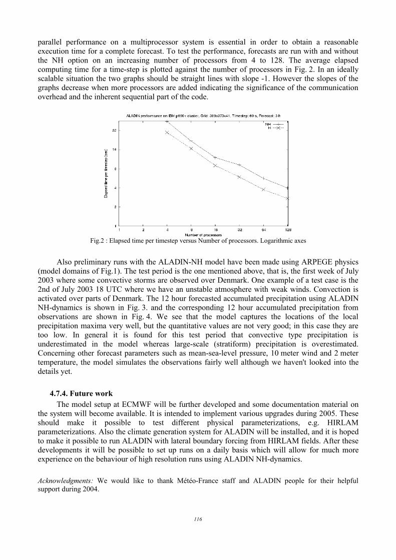
parallel performance on a multiprocessor system is essential in order to obtain a reasonableexecution time for a complete forecast. To test the performance, forecasts are run with and withoutthe NH option on an increasing number of processors from 4 to 128. The average elapsedcomputing time for a time-step is plotted against the number of processors in Fig. 2. In an ideallyscalable situation the two graphs should be straight lines with slope -1. However the slopes of thegraphs decrease when more processors are added indicating the significance of the communicationoverhead and the inherent sequential part of the code.

Fig.2 : Elapsed time per timestep versus Number of processors. Logarithmic axes

Also preliminary runs with the ALADIN-NH model have been made using ARPEGE physics(model domains of Fig.1). The test period is the one mentioned above, that is, the first week of July2003 where some convective storms are observed over Denmark. One example of a test case is the2nd of July 2003 18 UTC where we have an unstable atmosphere with weak winds. Convection isactivated over parts of Denmark. The 12 hour forecasted accumulated precipitation using ALADINNH-dynamics is shown in Fig. 3. and the corresponding 12 hour accumulated precipitation fromobservations are shown in Fig. 4. We see that the model captures the locations of the localprecipitation maxima very well, but the quantitative values are not very good; in this case they aretoo low. In general it is found for this test period that convective type precipitation isunderestimated in the model whereas large-scale (stratiform) precipitation is overestimated.Concerning other forecast parameters such as mean-sea-level pressure, 10 meter wind and 2 metertemperature, the model simulates the observations fairly well although we haven't looked into thedetails yet.

4.7.4. Future workThe model setup at ECMWF will be further developed and some documentation material on

the system will become available. It is intended to implement various upgrades during 2005. Theseshould make it possible to test different physical parameterizations, e.g. HIRLAMparameterizations. Also the climate generation system for ALADIN will be installed, and it is hopedto make it possible to run ALADIN with lateral boundary forcing from HIRLAM fields. After thesedevelopments it will be possible to set up runs on a daily basis which will allow for much moreexperience on the behaviour of high resolution runs using ALADIN NH-dynamics.

Acknowledgments: We would like to thank Météo-France staff and ALADIN people for their helpfulsupport during 2004.

116

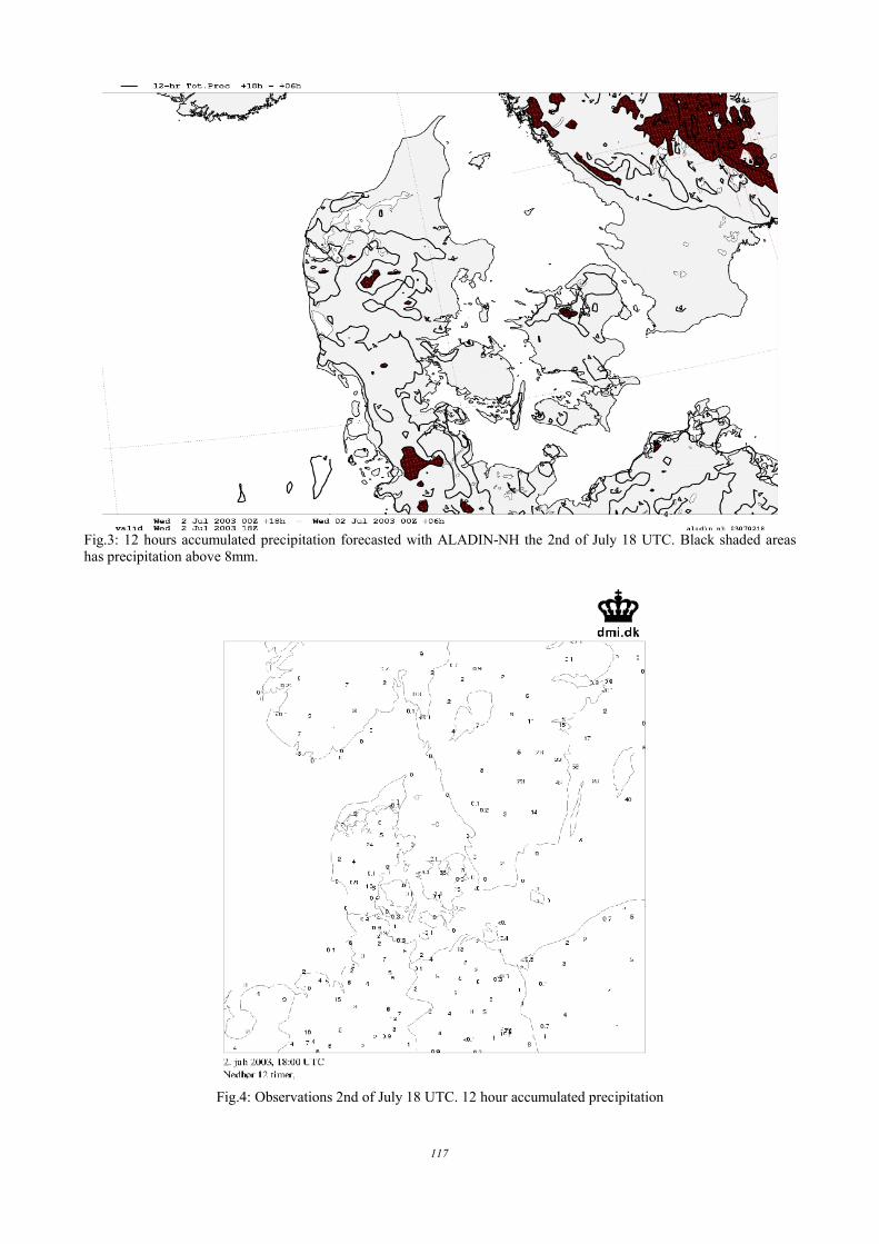
Fig.3: 12 hours accumulated precipitation forecasted with ALADIN-NH the 2nd of July 18 UTC. Black shaded areashas precipitation above 8mm.

Fig.4: Observations 2nd of July 18 UTC. 12 hour accumulated precipitation

117

4.8. Spline interpolation in semi-Lagrangian advection scheme of ALADIN/ARPEGE/IFS:Váňa Filip.

4.8.1. IntroductionMost operational NWP models are currently using for their advection computation the semi-

Lagrangian scheme. This scheme, among some other advantages, allows fairly longer time-stepswith respect to the Eulerian advection, while preserving the computational model grid contrary tothe pure Lagrangian solution. The price to achieve these nice features is typically to perform aninterpolation of advected fields at every integration time-step. The accuracy of such interpolation isthen a compromise given by need to keep it sufficiently precise and not too expensive with respectto the model performance. Typically, for most of the prognostic fields, this compromise is reachedby interpolation based on cubic polynomials (Staniforth and Côté, 1991).

The ALADIN/ARPEGE/IFS code uses for the purpose of the semi-Lagrangian "accurate"interpolation sort of 2D and 3D interpolators based on Lagrange cubic polynomial in destinationsclose to the target point and linear interpolation for the outer sphere (Yessad, 2004). Thisinterpolation works with sufficient efficiency and computational cost (Ritchie et al.,1995). Howeverits performance is limited by the performance of the Lagrange cubic interpolators, which tends to besometimes too stiff when applied to a rapidly changing quantity (field with dominating small-scalefeatures). This known limitation is already, on current operational scales for some fields, toorestrictive. Hence, for example, vertical interpolation for prognostic ozone can be optionallyperformed by spline (IFS) or by Hermite interpolators (ARPEGE/Climat). However the use of thosehigher order interpolations is restricted just to the vertical direction and prognostic ozone.

Since the semi-Lagrangian horizontal diffusion (SLHD) becomes a model feature, it hasimplicitly raised a need for more precise semi-Lagrangian interpolations. When SLHD is activatedthe original semi-Lagrangian interpolator is selectively corrupted by additional diffusiveinterpolation. Consequently the conservative ability of the advection scheme is deteriorated. It is aknown feature that, because of the inability to conserve total mass, the semi-Lagrangian modelsproduce generally a slight positive bias of surface pressure (Gravel and Staniforth, 1994). Thistendency is typically small enough that, especially for the purpose of NWP, it can be ignored. Thepresence of SLHD further enhances the positive mean-sea-level pressure (MSLP) bias tendencycaused by the semi-Lagrangian scheme.

This feature is illustrated by the figure displaying MSLP bias (lower lines) and rmse (upperlines) signals computed from a 19-days parallel test of ALADIN/LACE with SLHD (red colour) andwithout (black colour). The signal is not really dramatic and as proven it is even not furthercumulated within a continuous assimilation cycle using the results of previous runs as thebackground fields for the new analyses. Once again the conclusion can be that we can live with aslightly worse model performance in term of mass conservation having the benefit of relativelycheap non-linear horizontal damping.

118

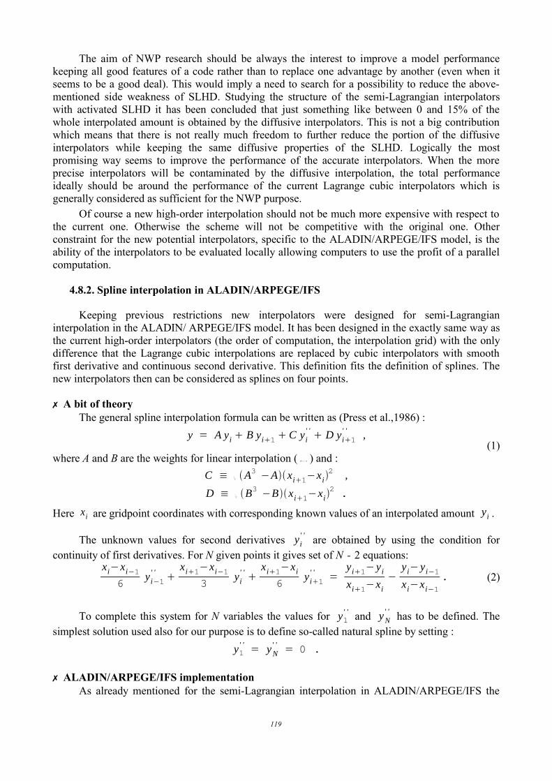
The aim of NWP research should be always the interest to improve a model performancekeeping all good features of a code rather than to replace one advantage by another (even when itseems to be a good deal). This would imply a need to search for a possibility to reduce the above-mentioned side weakness of SLHD. Studying the structure of the semi-Lagrangian interpolatorswith activated SLHD it has been concluded that just something like between 0 and 15% of thewhole interpolated amount is obtained by the diffusive interpolators. This is not a big contributionwhich means that there is not really much freedom to further reduce the portion of the diffusiveinterpolators while keeping the same diffusive properties of the SLHD. Logically the mostpromising way seems to improve the performance of the accurate interpolators. When the moreprecise interpolators will be contaminated by the diffusive interpolation, the total performanceideally should be around the performance of the current Lagrange cubic interpolators which isgenerally considered as sufficient for the NWP purpose.

Of course a new high-order interpolation should not be much more expensive with respect tothe current one. Otherwise the scheme will not be competitive with the original one. Otherconstraint for the new potential interpolators, specific to the ALADIN/ARPEGE/IFS model, is theability of the interpolators to be evaluated locally allowing computers to use the profit of a parallelcomputation.

4.8.2. Spline interpolation in ALADIN/ARPEGE/IFS

Keeping previous restrictions new interpolators were designed for semi-Lagrangianinterpolation in the ALADIN/ ARPEGE/IFS model. It has been designed in the exactly same way asthe current high-order interpolators (the order of computation, the interpolation grid) with the onlydifference that the Lagrange cubic interpolations are replaced by cubic interpolators with smoothfirst derivative and continuous second derivative. This definition fits the definition of splines. Thenew interpolators then can be considered as splines on four points.

✗ A bit of theoryThe general spline interpolation formula can be written as (Press et al.,1986) :

(1)where A and B are the weights for linear interpolation ( B=1−A ) and :

C ≡ 1

6A3 −A xi1−xi

2 ,

D ≡ 1

6B3 −Bxi1−xi

2 .

Here xi are gridpoint coordinates with corresponding known values of an interpolated amount yi .

The unknown values for second derivatives yi' ' are obtained by using the condition for

continuity of first derivatives. For N given points it gives set of N - 2 equations:xi−xi−1

6yi−1

' ' xi1−xi−1

3yi

' ' xi1−xi

6yi1

' ' =yi1− yi

xi1−xi

−yi− yi−1

xi−xi−1. (2)

To complete this system for N variables the values for y1' ' and yN

' ' has to be defined. Thesimplest solution used also for our purpose is to define so-called natural spline by setting :

y1' ' = yN

' ' = 0 .

✗ ALADIN/ARPEGE/IFS implementationAs already mentioned for the semi-Lagrangian interpolation in ALADIN/ARPEGE/IFS the

119

y = A yi B yi1 C yi' ' D yi1

' ' ,

"local" approach of spline is used so N will be always equal to 4. In such case with the natural splineboundary condition the equation (2) can be reduced to system of two equation for the two unknownsy2

' ' and y3' ' :

x3 −x13

y2 ' '

x3 −x26

y3 ' ' =

y3 − y2x3 −x2

−y2 − y1x2 −x1

x3 −x26

y2 ' '

x4 −x23

y3 ' ' =

y4 − y3x4 −x3

−y3 − y2x3 −x2

(3)

This set is always diagonally dominant when x2 −x1 ≠0 and x4 −x3 ≠0 , which isalways the case with the model grid. This means that a solution always exists as :

y2 ' ' =

C1 B2 −C2 B1

A1 B2 −A2 B1

,

y3 ' ' =

A1 C2 −C1 A2

A1 B2 −A2 B1

,

where :

A1=x3 −x1

3B1 =

x3 −x26

C1 =y3 − y2x3 −x2

−y2 − y1x2 −x1

,

A2 =x3 −x2

6B2 =

x4 −x23

C2 =y4 − y3x4 −x3

−y3 − y2x3 −x2

.

The horizontal interpolation can be fairly simplified by interpolating virtual functionF ' [ xi

' , yi ] instead of F [ xi , yi ] . Here the xi stands for general model computational grid whilexi

' represents virtual regular grid xi' − xi ≡ 1 . In case of ALADIN grid xi

' ≡ xi , hence F ≡ F ' .The two functions F and F' are illustrated by Figure 1. This trick is applied just to horizontal meshsince here the computational grid distribution is controlled by some rules (gauss grid, stretching)ensuring that the derivatives of an interpolated amount on the virtual grid would still somehowcorrespond with the computational grid. Vertical grid is determined by namelist without any a priorirestriction, so the interpolation is performed on the real grid along this direction. Fortunately thevertical interpolation is performed just once at the end of the 3D interpolation, so it is not causing adramatic increase of the model computational cost.

Fig.1: The true function F to be interpolated on stretched model grid fitting the model gridpoints (black full line with thepoints marked as diamonds) and the equivalent function F' transformed to regular grid which is interpolated insteadalong vertical during spline interpolation (red dashed curve with the points marked as stars). The target area to beinterpolated is located between points 1 and 2 on x-axis.

120

The equations (3) will have then for horizontal interpolation solution :y2

' ' = 2 54 y1 −9 y2 6 y3 − y4

y3' ' = 2

5−y1 6 y2 −9 y3 4 y4

In this case also the computation of the coefficients C and D in (1) can be simplified to just :C = 1

6A3 −A

D = 1

6B3 −B

Thanks to this simplification the computation of these interpolators is just around 2.8% more

expensive than the less exact Lagrange cubic interpolation4. There is still some space to furtheroptimise this performance, but it is questionable how much it would improve the final performance(i.e. it can happen that a lot of code-work will improve this performance by just negligible factor).

✗ User's guideTo switch the current Lagrange high-order interpolation to the one with splines in the

ALADIN/ARPEGE/IFS model is quite simple. A set of NAMDYN namelist switches calledLRSPLINE_[X] for separate variables (kind of variables) is defined to activate (when set to .T.)the spline interpolation :LRSPLINE_W for horizontal flow components LRSPLINE_T for temperature LRSPLINE_SPD for (NH) pressure departure LRSPLINE_SVD for (NH) vertical divergence LRSPLINE_P for continuity equation LRSPLINE_Q for moisture LRSPLINE_O3 for ozone LRSPLINE_V for other GFL fields

((Note that for ozone this spline interpolation has higher priority than quasi-monotone vertical spline interpolation(IFS), and both have higher priorities than vertical Hermite interpolators(ARPEGE/Climat).)

All the other features of the semi-Lagrangian interpolators like quasi-monotonicity (keysLQM [X]), horizontal quasi-monotonicity (keys LQMH[X]) or SLHD (key LSLHD) are preservedindependently to the actual value of LRSPLINE_[X]. The defaults values for cycle 29T1 are .F.,only in case of SLHD are LRSPLINE_W, LRSPLINE_T, LRSPLINE_Q and in case of NHdynamics LRSPLINE_SPD with LRSPLINE_SVD automatically set to .TRUE.

. 4.8.3. Performance of the splines

So what should one expect from the splines used instead of the Lagrange cubic interpolatorsdespite some increase of CPU time consumption ? Surely it is an improvement of the advectionscheme interpolation precision reducing a model random damping. This effect is reflected by thefigure 2, showing the response of interpolators to the kinetic energy spectra during an academicfrontogenetic idealised adiabatic 3D experiment with the model ALADIN (Vana, 2003). It isevident, that when spline is used instead of Lagrange interpolators, the inherent diffusion of thesemi-Lagrangian scheme is reduced especially for the small scale information.

4 This result was obtained with operational ARPEGE TL359L41c2.4 on Fujitsu VPP5000 and spline interpolation usedfor u, v, T, q but not s .

121

Fig.2: The kinetic energy spectra from the idealised adiabatic frontal development simulated with the model ALADIN asa result of used interpolators for semi-Lagrangian scheme. Black full line (1.5) represents the spline interpolation usedfor all interpolations (N[X]LAG=2), dashed red line(1.7) represents the same with the small difference that the tendencypart of the interpolated amount is interpolated by linear interpolation (N[X]LAG=3). Long dashed green line (2) isrepresenting the spectra obtained when Lagrange cubic interpolators is used exclusively for the whole semi-Lagrangianamount (N[X]LAG=2), dot-dashed blue line (3)represents the Lagrange interpolators used for fields while the tendencyare interpolated by linear interpolation(N[X]LAG=3). Finally dotted violet line (4) represents the result after just linearinterpolation.

Figure 3 shows the mean quadratic error of several interpolators with respect to the waves ofmodel spectrum (with quadratic truncation). As it can be seen the Lagrange interpolation isoutperforming the others for the long waves. Once the interpolated quantity becomes more rapidlychanging, the spline interpolators, fulfilling the additional conditions for derivatives, start tointerpolate with smaller error. This makes the spline interpolators especially profitable when somerapidly changing fields (of small scale character) will be advected.

Anyway some extensive validation to prove the response of the spline interpolation in term ofincrease of the computational precision of the model still has to be done. Up to now no parallel testfocused on this new model feature has been launched. Hence currently we can just speculate about apossible improvement of the model scores.

Other reason to use the splines in the ALADIN/ARPEGE/IFS model was linked to the SLHDdiffusion. To prove clear profit from the existence of spline interpolators for this case is relativelyeasy. As shown on the figure 4 the SLHD creates a systematic positive bias of the surface pressure.When the accurate interpolators of SLHD are spline ones, the positive bias tendency is significantlyreduced (the portion of areas with warm - yellow and red - colours is reduced). This reflects theability of the more precise spline interpolators to reduce the bias caused by semi-Lagrangianinterpolation.

122

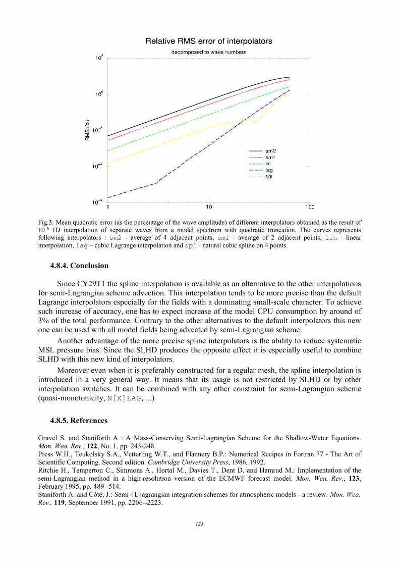
Fig.3: Mean quadratic error (as the percentage of the wave amplitude) of different interpolators obtained as the result of10 6 1D interpolation of separate waves from a model spectrum with quadratic truncation. The curves representsfollowing interpolators : sm2 - average of 4 adjacent points, sm1 - average of 2 adjacent points, lin - linearinterpolation, lag – cubic Lagrange interpolation and spl - natural cubic spline on 4 points.

4.8.4. Conclusion

Since CY29T1 the spline interpolation is available as an alternative to the other interpolationsfor semi-Lagrangian scheme advection. This interpolation tends to be more precise than the defaultLagrange interpolators especially for the fields with a dominating small-scale character. To achievesuch increase of accuracy, one has to expect increase of the model CPU consumption by around of3% of the total performance. Contrary to the other alternatives to the default interpolators this newone can be used with all model fields being advected by semi-Lagrangian scheme.

Another advantage of the more precise spline interpolators is the ability to reduce systematicMSL pressure bias. Since the SLHD produces the opposite effect it is especially useful to combineSLHD with this new kind of interpolators.

Moreover even when it is preferably constructed for a regular mesh, the spline interpolation isintroduced in a very general way. It means that its usage is not restricted by SLHD or by otherinterpolation switches. It can be combined with any other constraint for semi-Lagrangian scheme(quasi-monotonicity, N[X]LAG,...)

4.8.5. References

Gravel S. and Staniforth A : A Mass-Conserving Semi-Lagrangian Scheme for the Shallow-Water Equations.Mon. Wea. Rev., 122, No. 1, pp. 243-248.Press W.H., Teukolsky S.A., Vetterling W.T., and Flannery B.P.: Numerical Recipes in Fortran 77 - The Art ofScientific Computing. Second edition. Cambridge University Press, 1986, 1992.Ritchie H., Temperton C., Simmons A., Hortal M., Davies T., Dent D. and Hamrud M.: Implementation of thesemi-Lagrangian method in a high-resolution version of the ECMWF forecast model. Mon. Wea. Rev., 123,February 1995, pp. 489--514. Staniforth A. and Côté, J.: Semi-{L}agrangian integration schemes for atmospheric models - a review. Mon. Wea.Rev., 119, September 1991, pp. 2206--2223.

123

Vana F. : Semi-Lagrangian advection scheme with controlled damping - an alternative way to nonlinear horizontaldiffusion in a numerical weather prediction model. PhD thesis, Charles University Prague, 2003. In Czech withextended English and French abstracts.Yessad K.: Semi-Lagrangian computations in the cycle 29 of ARPEGE/IFS. Meteo-France/CNRM/GMAP/ALGOinternal memo, 2004.

Fig.4: The MSL pressure difference of 24 hours forecast of ALADIN/LACE with SLHD compared to the spectraldiffusion as reference (upper figure) and with SLHD + spline interpolation compared to the same reference (spectraldiffusion with default Lagrange interpolators) (bottom figure).

124

4.9. Impact of observations and tuning of observational error statistics: Chapnik Bernard. 4.9.1. Introduction

This short paper aims to sum up results obtained during a PhD supervised by OlivierTalagrand (CNRS/LMD) and closely advised by Gérald Desroziers and Florence Rabier(CNRM/GMAP) in Toulouse. Most of of the results were obtained in the French global ARPEGE4D-Var system.

The ever growing amount of available observations (among others, satellite data) reinforcesthe necessity of efficient tools able to evaluate the impact of each of them on the analysis ;moreover, proper statistics must be specified in order to retrieve as much information as possiblefrom those observations.

Most data assimilation scheme rely on linear estimation theory : the analysis (further denotedxa ) is fundamentally a linear combination of the background ( xb ) and of observations (y). From

this basis, it will be tried to answer to the following questions : • How to evaluate the impact of observations, or of a certain subset of the observations?• How to use this impact in order to tune a data assimilation system?

4.9.2. TheoryA short theoretical part will be useful to introduce the notations and concepts required in order

to answer those questions.

Let us first define an information vector z, zT = xbT yT , the vertical concatenation of the

background and the observation vectors. This vector is linked to the truth (x) by means of a linearoperator , T = I n

T H T : z = x , where H is the observation operator and is the

information error, concatenating background and observation errors T = bT o

T with

covariance matrix S = E T , where E is the expectation operator. In case observation and

background errors are not correlated, S is equal to B 00 R , where B and R are the background

and observations error covariance matrices.

The analysis xa is equal to : xa = xb K y − H xb , where K, the "gain matrix" can bewritten K = Pa H T R−1 , with Pa = B−1 H T R−1 H −1 which, in case the B and R matricesused in the system are the optimal matrices, is also the analysis error covariance matrix.

In variational data assimilation this analysis is obtained as the state vector minimizing anobjective function J (often called "cost function") :

J x = y −H xT R−1 y − H x x − xbT B−1x − xb ,

which, using the information vector can be rewritten : J x = z − x T S−1 z − x .If one supposes that this cost function can be split into several parts : J=∑ J i , with each Ji

written as : J i x = zi − i xT S i−1 zi − i x , z i is the ith subpart with dimension ni extracted

from the information vector z, associated with the i observation operator and the Si covariancematrix of its associated errors.

Then, if the specified covariances of the assimilation system really are the optimal matrices,

125

an important result provided by Talagrand (1999) applies. The expectation of the ith subpart of theobjective function at the minimum is :

E J i xa=ni−Trace i Pa iT S i

−1Moreover, Trace i Pa i

T S i−1 is a measurement of the contribution of zi to the overall

precision of the assimilation system.

A more explicit signification of these values can be obtained when focusing on thebackground/observations splitting of the objective function :- when z i=xb , Trace i Pa i

T S i−1=n−Trace KH , then E J b xa =Trace KH

- when z i= y , , Trace i Pa iT S i

−1=Trace HK , , then E J oxa =Trace I p−HK . ( I p isthe identity with order p)

It must be remarked that the use of the Trace of HK as quantification of the impact ofobservations had already be introduced by Wahba (1995) in a meteorological context. This quantityis called DFS, for Degrees of Freedom for Signal, see also Cardinali et al. (2004) for anotherexample of implementation of this diagnostic in a global data assimilation system.

Several points must be stated at this stage about DFS. DFS quantifies how the system uses theobservations to pull the signal from the background; in the optimal case (i.e K operationallyspecified = true K ), this is also the relative reduction of variance. Used on its own, DFS says whatthe system does, without any other criterion it cannot say what it should do in order to improve theanalysis.

A first clear problem appears : How do we compute DFS when K generally does not evenexplicitly exist in a variational scheme ? 4.9.3. Practical Computation of Trace (HK)

Two methods have been implemented in order to compute estimates of this Trace.✗ Girard’s method

The first method was proposed Girard (1987), it was introduced in the field of meteorologicaldata assimilation by Wahba (1995), and by Desroziers and Ivanov (2001).

The method is based on the following mathematical identity : considering a random vector εwith 0 mean and the identity covariance matrix, and an operator A, the expectation of the quadraticform T A is :

E T A=Trace AThis mathematical property is used as following :

- make a first "normal" analysis xa using the usual background and observations, - make a perturbed analysis xa

∗ using the same background and perturbed observations,y∗= yR0.5

It can easily be verified that the following scalar product approximates the wished quantity : y∗− yR−1H xa

∗−H xa˜ Trace HK

✗ The Simulated Optimal Innovations (SOI) methodThis method is introduced in Chapnik et al. (2005). It is based on the properties of subparts of

the optimal objective function at the minimum described in section 2. The algorithm consists in generating a situation, the errors of which are consistent with the

specified covariance matrices.

A state vector x (for example a background vector) is considered as the "truth". Adding

126

some noise, consistent with the specified statistics, a simulated background xb∗=xB0.5b and

observations y∗= yR0.5o are generated. The variational analysis of this simulated situation

naturally leads to the computation of J b xa∗ and of J oxa

∗ and of possible subparts of them.One then has :

J b xa∗≃Trace KH ;

J o xa∗≃Trace I p−HK ;.

The following equality : H xb∗−xa

∗T R−1 yo∗−H xa

∗≃Trace HK can also be applied inorder to compute subparts of Trace HK (this can only be applied if this subpart corresponds to adiagonal block of R ).

✗ Comparison of the two methodsFigure 1 compares the DFS computed for several upper atmosphere observation types on

4/02/2004 at 00 UTC within ARPEGE 4D-Var system. One may see that the results of the twomethods compare quite well. The small discrepancies observed, at least those larger than what canbe expected from randomized estimation methods (see the AMSU observations DFS, for example)may be explained by the non-linearities of the multi-incremental 4D-Var scheme used here. It canbe shown that even in this case, Girard’s method still evaluates a good estimate of the sensitivity ofthe analysis to the observations while the SOI method may be less accurate. 4.9.4. The tuning of variances

A way to use DFS (or a very similar quantity) to tune the specified statistics was provided byDesroziers and Ivanov (2001).

An hypothesis is made that the true optimal matrices can be obtained from the specifiedmatrices, just by multiplying them by multiplicative coefficients, the tuning coefficients; forexample, it may be supposed that Bt and Rt (the optimal background and observation errorcovariances) may be deduced from the specified B and R as:

Bt=sb BRt=so R

Supposing the system is variational, if J o and J b are the subparts of the objectivefunction related to xb and y respectively then J opt=J o/ soJ b/ sb is the optimal objective function.The criterion of the expectation of subparts of the objective function at the minimum must thenapply. Let xa be the minimizer of J opt ; replacing the expectation operator by one realization(which in case there are enough observations is justified) yields the following criterion to determineso and sb:

J b xa so , sb/ sb=Trace K so , sbH ;J o xa so , sb¿/ so=Trace I p−HK so , sb ..

The notations used here are to emphasize the fact that xa and K are functions of so and sb.Those equalities are easily transformed into:

so=2 J oxa so , sb/Tr I p – HK so , sbsb=2 J b xa so , sb/Tr K so , sbH

This set of equation is a fixed-point relation so , sb= f so , sb . A fixed-point algorithm isthen applied to compute so , sb . The Trace term can be computed with Girard’s method, but withthe SOI method the previous relations become

so=J o xa so , sb/ J oxa∗so , sb ;

sb=J bxa so , sb/ J bxa∗so , sb .

127

xa∗ is the analysis made from the simulated situation defined in the presentation of the SOImethod. These expressions outline that the method compares "true" and "simulated" statistics. Anadvantage of the SOI method is that the numerator and the denominator of these expressions can beobtained in the same way.

A nice property of the algorithm is that the first iteration of the fixed point used hereconverges very quickly. The first iteration generally provides a good estimate of the result andconvergence is generally reached after two or three iterations, except for cases that are going to bedefined in the next section. 4.9.5. Properties of the method✗ Equivalence to Maximum Likelihood Tuning

It may be shown (Chapnik et al 2004) that the tuning performs a Maximum Likelihood tuningof variances (see Dee and da Silva 1998 for meteorological use of Maximum Likelihood in dataassimilation), meaning that the tuning coefficients are the most probable coefficients, considering ana priori model of covariance (the specified B and R matrix) and the data (in our case theinnovation, obs-guess difference). This has important consequences for the tuning :

Since the method performs a statistic over he innovation, a large innovation vector, therefore alarge observation vector, is needed.

An a priori hypothesis about the structure of correlations, allowing to split the innovation intoobservation and background errors is necessary (like in Hollingsworth and Lönnberg, 1986). Thishypothesis is in HBH T and R (the a priori specified matrices) which must be different (e.g. nospatial correlation in R , spatial correlation in B ) to allow a useful tuning.

If this hypothesis is not (even roughly) respected by the true o and b , a poor tuning maybe expected. In particular, performing the method on an observation type with spatially correlatederrors represented with a diagonal R yields a very weak, possibly null so , which is the oppositeof what should be done in this case (inflate the optimal o ). Note that a non optimal correlationlength in B does not have such bad consequences.

✗ A first try with real dataA first try is made to check in a first time if the tuning coefficients have a priori desirable

properties they should have. Desroziers and Ivanov (2001) had already shown the ability of themethod to retrieve the tuning coefficients for a simulated case in a comprehensive data assimilationsystem. The consistency between the tuning coefficients and the known quality of the observationsis tested here.

Figure 2 shows the tuning coefficients computed for satellite borne instruments channels, in1997 and in 2001. One may clearly see that small coefficients remain small and that largecoefficients remain large over four years. Moreover, the variability between the two dates is of thesame order as the one encountered when comparing the tuning coefficients computed at differentdates of the same month (not shown). Such a behaviour is a positive point if we suppose that therewere no major evolution of the quality of the observation between the two dates; yet, evidence thatthe result is not an artifact is still needed, evidence that the same result will not be obtainedindependently of the o of the observation errors. A known dysfunction of NOAA 15 instrumentswas the occasion to document this point. Figure 3 shows the tuning coefficients obtained for threechannels on dates when there were no problems (dashed black and white bars), on the day before theproblem begins (green bars), and during the incident (the other bars). It is clearly seen for two of thechannels that the tuning coefficients are multiplied by two (and even more on the last date) duringthe incident. The tuning coefficients are clearly related to the quality of the observations.

128

4.9.6. Impact of the tuning of the varianceThe final point of this study is the assessment of the tuning of the specified observational error

variances on the analysis and on the forecasts.In a first time the tuning was performed for the assimilated observation types. For

observations known to have very correlated observation errors (like SATOB observations), thetuned values were taken similar to the specified values (the true tuned values dropping to 0 alongthe tuning as noticed in section 5). A single coefficient was applied to tune B , and was foundequal to 1, meaning that, as a whole, B was approximately correct.

An experiment was carried out, performing an analysis cycle for 20 days with the "tuned"analysis system. Figures 4a-c compare the rms differences between geopotential observations andforecast, for "tuned" forecasts and operational forecasts. The green lines denote improvements ofthe rms, the red ones show a deterioration. It can be seen that for this parameter, the impact ispositive for all forecast ranges. For other parameters, the impact, though positive, may be lessspectacular. 4.9.7. Conclusion

Techniques to evaluate the quantification of the impact of the observations, known as DFS,have been implemented for the French ARPEGE data assimilation system. These techniques canalso be used for Desroziers and Ivanov’s tuning of the variances. This tuning has been shown tohave some positive impact on the analysis and on the forecasts.

The first future direction which might be taken is the tuning of the B matrix. As stated before,only one global coefficient was applied to this matrix, which is certainly not enough. Severalstrategies for a finer tuning may be considered.

Another difficulty to be considered in the future is the tuning of observations with correlatederrors (like SATOB). This case is more difficult since no known objective criterion allowing to tuneit can apply. 4.9.8. ReferencesC. Cardinali, S. Pezzuli and E. Andersson Influence Matrix diagnostic of a data assimilation system. Proceedingsof the Seminar on Recent developments in data assimilation for atmosphere and ocean, ECMWF, Reading, 8-12September 2003. B. Chapnik, G. Desroziers, F.Rabier and O.Talagrand. 2004, Properties and first applications of an error statistic tuningmethod in variationnal assimilation. Quart. J. Roy. Meteor. Soc., 130, no. 601, pp. 2253-2275B. Chapnik, G. Desroziers, F. Rabier, and O. Talagrand. 2005, Diagnosis and tuning of observational errorstatistics in a quasi operational data assimilation setting. Accepted with minor revision by Quart. J. Roy. Meteor.Soc.G. Desroziers and S. Ivanov. 2001, Diagnosis and adaptive tuning of information error parameters in a variationalassimilation. Quart. J. Roy. Meteor. Soc., 127, 1433-1452. D. Dee and A. da Silva. 1998, Maximum likelihood estimation of forecast and observation error covarianceparameters. part I: Methodology. Mon. Wea. Rev., 124:1822--1834.D. Girard. 1987, A fast Monte Carlo cross-validation procedure for large least squares problems with noisy data.Technical Report 687-M, IMAG, Grenoble, France.Hollingsworth and Lonnberg, 1986: The statistical structure of short-range forecast errors as determined fromradiosonde data. Part I : the wind field. Tellus 38A, 111-136.O. Talagrand. 1999 A posteriori verification of analysis and assimilation algorithms. In Proceedings of theECMWF Workshop on Diagnosis of Data Assimilation Systems, pages 17--28, Reading, November 1999. G. Wahba, D. R. Johnson, F. Gao and J. Gong, 1995: Adaptive tuning of numerical weather prediction models:randomized GCV in three and four dimensional data assimilation, Mon. Wea. Rev., 123, 3358-3369.

129

A IR E P _ T

A I R E P _ U

A M S U

S A T O B

P I L O TT E M P _ Q

T E M P _ T

T E M P _ U

0

1 0 0 0

2 0 0 0

3 0 0 0

l at > 20°

- 20 ° < l a t < 2 0°

l at < - 20 °

0

1 0 0 0

2 0 0 0

3 0 0 0

SOISOI

GirardGirard

Figure 1 : DFS computed for different observation types. The bars in blue were computed with Girard's method, bars inred with the SOI method. Each bar is divided into three parts: the upper part is the contribution of observations from thenorthern hemisphere; the middle part is the contribution from subtropical observations ; the lower part, the contributionfrom the southern hemisphere.

0

0.5

1

1.5

2

2.5

3

3.5

4

4.5

HIRS1 HIRS2 HIRS3

29-Jun6-Jul13-Jul27-Oct28-Oct29-Oct30-Oct

Figure 2 : Comparison between tuning coefficientscomputed on a 1997 date (in red) and a date in 2001 (inblue), for different satellite channels (along the x axis).

Figure 3 : Detection of an incident. Tuning coefficientscomputed for dates before the incident (dashed greybars),the day before the incident (green bars), and duringthe incident (orange, purple and red bars).

130

a b cFigure 4 : Difference between the rms (geopotential TEMP observations minus forecast) for operational forecasts and"tuned" forecasts. The unit is the meter. Green lines show an improvement, red lines a deterioration. The x axis is therange of the forecast, the y axis is the pressure level. Panel 4a is for inter tropical areas, panel 4b for the southernhemisphere and panel 4c for the northern hemisphere.

4.10. Adaptations to ALADIN of the Lopez micro-physical package: Gérard Luc.

4.10.1. IntroductionOur ongoing development of a parametrization set combining the convection with other moist

physical schemes required to get a suitable micro-physical package.We started from the one developed by Ph. Lopez (2002) in the frame of ARPEGE-Climat, and

dedicated to "resolved" or "stratiform" clouds and precipitation. 4.10.2. Original scheme

The original Lopez scheme uses two prognostic variables : a total specific cloud condensateqc and a total specific precipitation content qP . However, in each of the micro-physical routines, a

diagnostic phase partition is estimated. For the condensate, it assumes a progressive transition of theice fraction between two temperatures (e.g. -10 and -40 °C). For the precipitation, a nearly steptransition at 0 °C is considered (actually it may extend over several levels to avoid that theassociated cooling brings the local temperature below 0°C).

The package works as follows :1) A resolved condensation scheme, base on Smith (1990), yields a condensate tendency and a

resolved cloudiness.2) This tendency is added to the original condensate content (advected from the previous time-step),

to yield a transitional value before precipitation.3) A parametrization estimates the rate of auto-conversion of this condensate to precipitation.4) The auto-converted part is subtracted from the condensates and added to the prognostic

precipitation content, which is then advected vertically in a semi-Lagrangian way. Theinstantaneous qP as well as the total precipitation crossing a layer in one time-step are used tocompute the precipitation evaporation and the collection of the cloud condensate by theprecipitation. For the latter, one distinguishes the aggregation of cloud ice by snow, the accretionof droplets by rain, and the riming of droplets by snow.

5) Some corrections may be brought to the tendencies of the water specific contents to prevent theoccurrence of negative values.

The package implied to adapt the expression of the tendencies, to include additional fluxes :condensation fluxes, precipitation evaporation fluxes, both with their associated heat fluxes; aprecipitation melting heat flux, and fluxes associated to the precipitation content evaluation : a fluxof precipitation generation, and a flux of precipitation evolution, including the different processes

131

they experience during their fall.The progress of our scheme led us to make several adaptations to the original routines.First, it appeared advisable to use separate model variables for cloud ice and liquid water. This

distinction is essential for radiative properties, and for further refinements of the micro-physicaldescription. At the same time, the use of a full prognostic variable (advected by the mean modelwind) for precipitation content seemed less important. In a first step, we replaced it by a pseudo-historic variable, i.e. a passive memory of the values from the previous time-step, with no resolvedadvection. Later, we found it better to suppress completely the precipitation content (see below).Using separate model variables for cloud ice and liquid water implied to reassess the treatment ofthe mixed phase : each of the different micro-physical processes tends to modify the phase partition,so that we must care for restoring it at the end, to prevent an unrealistic situation.

We were also confronted to some flaws or hidden approximations in the original scheme.Seen the difference in phase partition for cloud particles and precipitation, cloud droplets may beconverted (either by auto-conversion or riming) into falling snow : the released latent heat was nottaken into account.

The semi-Lagrangian vertical advection of the precipitation content posed several problems.The auto-conversion is applied at once at the beginning of the time-step, instead of considering acontinuous feeding. It is possible that some layers directly below the cloud receive zero advectedcontent, because the origin of the trajectory is above the cloud. On the other hand, the evaporationcalculation is based on the total precipitation crossing the layer, and applied to the final advectedcontent. When the latter is zero, it results into a negative final content. The problem is that theevaporation should be based on the conditions along the trajectory, not at the arrival point. Finally,the resulting precipitation contents could not be directly related to the precipitation fluxes, whichposed serious conceptual problems for introducing a downdraught calculation.

4.10.3. Scheme adaptations✗ The condensation scheme

A peak of condensation was observed near the 0° C isotherm, associated to the cooling by themelting of the precipitation. To limit this, a smoothing of the temperature profile around the level ofthe triple point may be applied; the number of levels above and below may be chosen in thenamelist.

Unwanted condensation could also occur near the lowest model level, consecutive to thecooling by the downdraught. We introduce the possibility to use there the arithmetic mean with thesurface temperature, which in this case is higher than the air temperature.

✗ The auto-conversion routineThe rather intricate calculation coded by Lopez has been replaced by a more transparent

formulation.An integrated Kessler formula yields the decrement of cloud water content due to auto-

conversion. For liquid condensate ql , it writes:

ql = qlx 1−e

E l t if ql ql

x

where E l is the auto-conversion efficiency for droplets. In presence of ice, the threshold for liquidauto-conversion ql

x is lowered to zero. Subsequently, an auto-conversion gain GWBFAUT, associated to the Bergeron-Findeisen

mechanism is applied :ql =ql

x 1 GWBFAUT⋅E l⋅i

132

where i is the ice fraction in the cloud. In the mixed phase, the ratio of water to ice must be maintained, so that the final ice content

may be derived from the final liquid content. In the pure ice phase, a Kessler integrated formula alsoholds, but the auto-conversion efficiency is made dependent on the temperature. We introducedadditional parameters to tune this dependence.

4.10.4. The precipitation routineGiven the above-mentioned problems with the precipitation advection routine, we proposed a

simpler and more clearly justified approach.The auto-conversion alone yields a gross precipitation flux Pau (which may also include a

pseudo-historical flux memorized from the previous time-step), from which we derive : • the total precipitation crossing the layer in one time-step :

qPtot=Pau

g t p

(this makes the hypothesis that the precipitation generation varies slowly enough in time so thateven the lowest layers are crossed by a flux corresponding to the present auto-conversion in thelayers above)

• the instantaneous densities of snow and rain in the layer :

Ps=Pausnow

wPs

and Pr=Pau 1−snow

wPr

,

where wPs and wPr are the fall speeds of snow and rain, which are assumed constant and maybe chosen in the namelist, snow is the solid fraction of the precipitation.

These quantities allow to compute first the evaporation/sublimation processes, and afterward, thedifferent collection processes.

We now consider that the evaporation/sublimation, occurs in the clear part of the grid box, butonly the part of it under a "precipitating" area, which can be estimated from the cloud fractions atdifferent levels. In the original scheme, the same collection efficiency was assumed for aggregationof ice and riming of droplets by falling snow : we introduced separate tunings.

✗ The final corrections.An adaptation of the mixed phase composition is performed after the precipitation. It implies

a melting/freezing flux and an associated heat flux, between solid and liquid condensate.The adaptation of the tendencies to prevent negative specific contents has been adapted to :

• extend the treatment to the cloud water variables, • forbid cloud ice above the triple-point temperature.

4.10.5. ConclusionsMost adaptations described above appeared useful or necessary during our work on the

integrated scheme for clouds, precipitation and convection, after controlling the profiles andbehaviour of the cloud water phases or other associated variables.

We think to have got a more realistic behaviour, together with a reduction of the cost, mainlyby suppressing the heavy advection calculation. Now more systematic tests and comparisons shouldbe performed to validate the adapted package. 4.10.6. ReferencesPh. Lopez: Implementation and validation of a new prognostic large scale cloud and precipitation scheme forclimate and data assimilation purposes, Q. J. R. Meteorol. Soc., 128 (579), 229-258, 2002.

133

R. N. B. Smith: A scheme for predicting layer clouds and their water content in a general circulation model, Q. J.R. Meteorol. Soc., 116, 435-460, 1990.J. C. H. van der Hage: A parametrization of the Wegener-Bergeron-Findeisen effect, Atmos.Res.,39, 201-214, 1995.

4.11. VARPACK– A diagnostic Tool, based on the 3DVar/ALADIN surface scheme: AugerL & Taseva L.

4.11.1. IntroductionThe purpose of this work on Varpack was to study the possibility of implementation of the

ALADIN/3DVar scheme for diagnostic and nowcasting purposes. Such a software would havebeen an analogue of Diagpack, based on the CANARI OI scheme. The first tests with the Varpacksoftware have been performed early 2004 and a comparison with Diagpack has been done. Theresults have shown that Diagpack and Varpack give similar meteorological fields and there is apossibility to improve the application of the ALADIN 3D-Var scheme as a diagnostic tool (Auger,2004; Taseva and Auger 2004). During the Summer of 2004, the ALADIN/3Dvar scheme has beenmodified by introducing the difference (Ts – TN) where N is the lowest model-level, as a newcontrol variable (Auger 2004b). The tests with Varpack performed late 2004 have shown that thereis a significant advantage of the new Varpack with respect to the old one (Taseva and.Auger 2004b).

In Section I the results of the comparison between Diagpack and Varpack are presented, whilethe results of the experiments with Varpack are presented in Section II.

4.11.2. Section I – Basic features of Diagpack and Varpack

✗ Diagpack

With Diagpack an operational hourly CANARI OI analysis is performed with:• a first guess field from ALADIN forecasts (from 3 to 8 h ones)• surface data, obtained from manual and automatic land and ship SYNOP stations.

When running Diagpack, some constrains are applied: • only the stations below the altitude of 1500 m are used in the analysis;• the stations, for which the difference between the model orography and the altitude at the

observation point is bigger than 800 m, are not assimilated.The observation operators allow performing an upper-air analysis of geopotential, temperature

and humidity at the model levels up to approx. 1500m only with SYNOP observations and a directanalysis of T2m, RH2m, V10m. Those fields together with the diagnostic parameters CAPE andMOCON, computed by specific post-processing options, are used afterwards for nowcastingpurposes (CAPE computed from analysed 2m fields, mainly NFCAPE=4, MOCON calculated asdiv(q2mV10m).

✗ Varpack (2004)

We used all the SYNOP data that passed through ALADIN screening to performtemperature, wind and specific humidity analysis on model levels only.

Three different modifications of the basic 3DVarc onfiguration scheme were tested :• The value of the model standard deviation error (i.e. The scaling factor REDNMC) has been

increased to better fit observations, this version is referred as Varpack/bas3D.

134

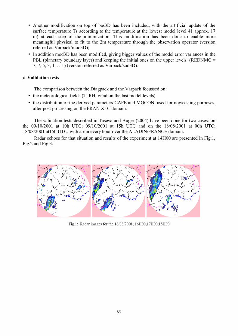
• Another modification on top of bas3D has been included, with the artificial update of thesurface temperature Ts according to the temperature at the lowest model level 41 approx. 17m) at each step of the minimization. This modification has been done to enable moremeaningful physical to fit to the 2m temperature through the observation operator (versionreferred as Varpack/mod3D);

• In addition mod3D has been modified, giving bigger values of the model error variances in thePBL (planetary boundary layer) and keeping the initial ones on the upper levels (REDNMC =7, 7, 5, 3, 1, …1) (version referred as Varpack/sod3D).

✗ Validation tests

The comparison between the Diagpack and the Varpack focussed on:• the meteorological fields (T, RH, wind on the last model levels)• the distribution of the derived parameters CAPE and MOCON, used for nowcasting purposes,

after post processing on the FRAN X 01 domain.

The validation tests described in Taseva and Auger (2004) have been done for two cases: onthe 09/10/2001 at 10h UTC; 09/10/2001 at 15h UTC and on the 18/08/2001 at 00h UTC;18/08/2001 at15h UTC, with a run every hour over the ALADIN/FRANCE domain.

Radar echoes for that situation and results of the experiment at 14H00 are presented in Fig.1,Fig.2 and Fig.3.

135

Fig.1: Radar images for the 18/08/2001, 16H00,17H00,18H00

Fig.2: Cape for Diagpack (top left), Varpack experiment mod3d (top right) and Varpack experiment sod3d (bottom) forthe 18/08/2001 at 14H00.

136

Fig.3: MOCON for Diagpack (top left), Varpack experiment mod3d (top right) and Varpack experiment sod3d(bottom) for the 18/08/2001at 14H00.

It can be seen that:• MOCON fields derived from Varpack, are very similar to those derived from Diagpack, but

smoother;• CAPE fields derived from Diagpack and Varpack are quite different, both giving on that case,

a quite poor diagnostic for future convective events.

137

4.11.3. Section II – Experiments with Varpack

During the summer of 2004, the ALADIN 3D-Var surface scheme has been modified byintroducing the vertical temperature difference between surface and the lowest model-level (Ts –TN) at the observation point as a new control variable in the vector. This modification, made by L.Auger has been validated by comparison with Diagpack and the previous version of Varpack . ✗ Basic ideas of the new 3D-VAR/ALADIN surface scheme - surface temperature in the

control variable.

In the 3D-VAR formalism, the goal is to minimize a coast function:

Where: d= y−H xb is the departure between the observation vector y and the modelequivalent computed from the background xb and x is the control variable.

The goal of the algorithm is to minimize the J cost function with respect to x .

So far in ALADIN 3D-VAR only upper-air fields were used inside the control variable.But, when analysing 2 meters observations, one needs to be able to modify during the

minimization cycle also the surface variables, because the observation operator H is using surfaceparameters to compute the model equivalent at 2 meters or 10 meters.Let's call T S the surface temperature departure (actual temperature minus background temperature)and T N the lowest level temperature departure.

The difference T S−T N was introduced as a new control variable. To this new controlvariable was associated a forecast error standard deviation T S−T N

representing the error made bymodel on this parameter. So the new model error cost function reads:

Introducing T S−T N as a control variable, provides a correlation between the surface and thelowest level temperature without having to modify the B matrix structure (model forecastcovariances error). The main problem when using a B matrix which would include surfaceparameters is that in ALADIN, upper-air fields are specified in spectral space whereas surface fieldsare specified as gridpoint ones. It also seems difficult to compute a reliable B matrix near theground because the model forecast error inside the boundary layer might be quite important.

More details are given in Auger (2004b).Only this new version will be considered hereafter.

✗ Results of the experiments for the case study 2004/10/09

That case has been chosen because the CAPE obtained by Diagpack at 12H00 indicated apotential for a storm, that developed in the following hours.

To create a reference run, the new ALADIN/3D-VAR surface scheme has been modified to beconsistent with the settings of Diagpack :

• the data base included only the observations within the 10 minutes interval around theobservation time,

138

J=J bJ o=1 2

xt B−1 x1 2

H x−d t R−1H x−d

J b=1 2

xt B−1 xT S−T N tT S−T N

−2 T S−T N

• the old blacklist was modified by excluding the French RADOME observations from it, • smaller values of the observation errors were set, • the operational 6-hour ALADIN forecast was taken as first guess, • the ALADIN/3D-VAR surface scheme was modified with a complete de-correlation of the

temperature and humidity, and a new executable had been created, • in screening and minimization the default values of RGBQC were taken,• in minimization with LTSCV=. T. (LTSCV is the new logical flag for activating the Ts

control variable) the value TSCVER=0.5 was used,• in minimization model error covariances were inversed in PBL;• in forecast no DFI were applied, • in FullPos CAPE was computed from the lowest model-level (NFPCAPE=1) or from

meteorological standard height after the computation (NFPCAPE=3).

The analysis of the diagnostic JOT tables before screening, before and after minimizationhave shown that :

• screening had rejected mainly U10 observations for all subtypes of SYNOP data (11-landmanual report, 14-land automatic report, 15-French automatic land report, 16-FrenchRADOME);

• the result of the minimization is a state, close to the observations – the values of thenormalized JO/n have decreased an order of magnitude for all SYNOP subtypes and allvariables.

Fig.4 : Radar data for 20041009, 16H00 and 17H00.

139

Fig.5: Time evolution of CAPE, derived by Diagpack (top left), new Varpack with NFPCAPE=1 (top right) and withNFPCAPE=3 (bottom)

On radar images (Fig. 4) we can see that a strong convective event starts at 16H00 UTC onthe South-West part of the domain. On the CAPE diagnostic from Diagpack (Figure 5), we have astrong signal at 12H00 at the same location, proving the convective capacity of the atmosphere atthat place, leading to the development of the storm a few hours later.

On Figure 5 (top right and bottom panel), the Varpack diagnostic is not so good, it showsmore maxima at some places where no rain event was observed later.We can also observe that the CAPE computation with NFPCAPE=1 and NFPCAPE=3 givessomehow different CAPE fields, although there is a lot of common pattern between the twopictures.

140

Fig.6: 2m temperature analysis by Diagpack (left) and temperature at the last model level for Varpack.

Figure 6 presents the 2m temperature field, obtained by Diagpack, and the one (at the lowestmodel level (41), obtained by Varpack at 12H00. It can be seen that there is a good agreementbetween the two temperature fields even if level 41 corresponds approx. to 17 m height. For that daythe boundary layer is quite well mixed so temperature at 17m is not much different fromtemperature at the ground.

Fig.7: Relative humidity at 2m for Diagpack (left panel), relative humidity at the lowest model level, recomputed fromtemperature and specific humidity, with correction from MSL pressure, obtained by Varpack (2004b) (right panel).

The humidity fields from Diagpack and Varpack (Figure 7) are also very similar, except formountainous areas.

It is seen that:• there are small differences for temperature and relative humidity for most part of the domain.• these minute differences explain the differences between the CAPE fields obtained by

Diagpack and Varpack, mainly because CAPE is very sensitive to the temperature andhumidity at the starting point in the integral computation.The comparison with the observed values of 2m relative humidity (Hu 2m)have shown that

when there are no observations in an area with a characteristic size of 50 km, Diagpack is givingmuch importance to the guess and produces a poor diagnostic of Hu 2m, whereas for such cases,

141

the Varpack analysis gives a relative humidity field that seems to be in better agreement with reality.

4.11.4. Impact of the observations for altitude stations.

On the specific case shown before, the CAPE diagnostic from Diagpack enabled a goodforecast of the storm that develops at 16H00 UTC.

Looking more carefully at the temperature and humidity analysis provided by Varpack, wesaw that one station at 600 m gave a quite different increment analysis for T2m and Hu2m on theSouth-East part of the domain.

This is because there is no horizontal correlation between our control variables (Ts-TN) atdifferent observation points. As a matter of fact, unplugging the modification of the control variablein that specific case gave a CAPE diagnostic that is much closer than the Diagpack CAPE (Fig.8).

Fig.8: CAPE diagnostic from Varpack, for the 09/10/2004 at 12H00, without the modification concerning the controlvariable. 4.11.5. Section III. Conclusions and intents for the future work

The main conclusions, reached on the basis of the performed experiments in Section I andSection II are as follow:

• there is a significant advantage of the new Varpack version with respect to the previous one(Auger 2004). Besides, the results are scientifically more satisfying due to the new controlvariable (Ts – TN),

• The temperature fields obtained by Diagpack and Varpack are similar,• the humidity fields obtained by Diagpack and Varpack are a little different. For most of the

142

cases we looked at, the ALADIN/3D-VAR humidity analysis seemed at least as good asDiagpack one, in comparison with the 2 m observations,

• the CAPE fields derived from Diagpack and Varpack are still different, mostly because somealtitude observations have a different impact But as the CAPE field is used for convectiveactivity diagnostic and is not 100% reliable, it is difficult to evaluate its quality on a fewcases,

• MOCON fields derived from Diagpack and Varpack are close.

The further study of Varpack analysis requires• to study more the Varpack humidity analysis,• to study the possibility of using new observation types,• to correct the problem linked with altitude station impacts.

4.11.6. Acknowledgements

The authors are mostly grateful to F. Taillefer and F. Bouyssel for their help in performingthe experiments and in the discussion of the obtained results.

4.11.7. References

AUGER L., 2004: Analyse diagnostique de type variationnel (Diagnostic analysis with variational method).Internal Workshop (07.05.2004), Météo - France,Toulouse, France.AUGER L., 2004b: 3D-Var surface assimilation for diagnostic purposes. SRNWP/Met Office/HIRLAMWorkshop “High-resolution data assimilation: towards 1- 4 km resolution” (15th - 17th Nov 2004), Met Office,Exeter, UK.TASEVA L. and L. AUGER, 2004: VARPACK. Technical Report (June 2004), Météo-France/CNRM/GMAP,Toulouse, France. http://www.cnrm.meteo.fr/aladin/publications/report.html TASEVA L. and L.AUGER, 2004b : Varpack, based on the new version of the 3D-Var/ALADIN surfacescheme. Technical note (November 2004), Météo-France/CNRM/GMAP, Toulouse, France.

4.12. An update on the 2002 Gard flood simulation with the ALARO-10 prototype in 2004:A comparison between ALADIN, Méso-NH, ALARO-10 and AROME: Hello Gwen.

4.12.1. Summary In summer 2004, some preliminary testing was run using a model consisting of the AROME

prototype software at 10-km resolution plus a subgrid convection scheme. This model is called"ALARO-10" in this paper although the contents of the ALARO-10 subproject changed in 2005.Preliminary results from the tests were shown on four cases. Runs on the Gard case were publishedin ALADIN Newsletter 26. Later, in December 2004, it turned out that the precipitation diagnosticsfrom these runs were incorrectly interpreted : the displayed cumulated rainfalls did not include thecumulated rain coming from the parametrized convection. That is the reason why there was too littlerainfall in the output of ALARO-10. This article shows the new results with the corrected ALARO-10 runs on the GARD case.

The Gard case is a very extreme meteorological flood event over the South-East of France, itis also a major case for the qualification of the AROME prototype.

143

4.12.2. Characteristics of the different runs used The GARD case is a 12 hours forecast run, starting on 08/09/2002 at 12 UTC and ending on

09/09/2002 at 00 UTC.✗ ALADIN-oper

The characteristics of the ALADIN-oper runs are the same as ALADIN-France operational inSeptember 2002 (i.e. not the present operational physics) :

• Semi-Lagrangian dynamics with 2 time-levels, hydrostatic formulation• Time-step = 415,318s (7 minutes), x = 9.5 km, 41 vertical -levels and coupling every

3h to ARPEGE.✗ Méso-NH

• Eulerian dynamics with anelastic formulation• Time-step = 15s, x = 10 km, 41 vertical z-levels and coupling every 3 hours to

ARPEGE.• Radiation scheme: RRTM, convection scheme: KFB (called every 5 minutes),

externalised surface, complete micro-physics with prognostic water variables, andprognostic turbulent kinetic energy.

✗ ALARO-10• Semi-Lagrangian dynamics with 2 time-levels, hydrostatic formulation.• Time-step = 60s, x = 10 km, 41 vertical -levels and coupling every 3 hours to

ARPEGE• Same physics as Méso-NH except that the convection scheme is called every time-step.

✗ AROME• Semi-Lagrangian dynamics with 2 time-levels, non-hydrostatic formulation with a PC

(ICI) scheme.• Time-step = 60s, x = 2.5 km, 41 vertical -levels and coupling every 3 hours to

ALADIN-France or Méso-NH.• Same physics as Méso-NH or ALARO-10, but no convection scheme (the convection is

assumed to be resolved).•

4.12.3. Results✗ Boundary layer fields

We look there at temperature at 2 m and wind at the lowest level for the different models.Observed 2 m temperature and 10 m winds are also shown.

- 2m temperature field The 2m temperature field on the 09/09/2002 at 00 UTC shows a cooling under the

thunderstorm. This is an important feature of this case. The cooling area is outlined on the followingfigure (Fig. 1) with T2m observations.

144

Fig.1: Observations of 2m temperature on 09/09/2002, 00 UTC, on Southern France.

a) c)

b)

Fig.2: 12 h forecasts of 2 m temperature, valid at 09/09/2002 00 UTC.a) ALADIN-oper (x = 9.5 km), b) ALARO-10 (x = 10 km), c) Meso-NH (x = 10 km)

The cooling is seen by the several models : Méso-NH at 10 km, ALARO-10 and ALADIN-oper, the corresponding 12 hours forecasts are show on Figure 2. The minimum temperature in thecooling area is 10°C for Méso-NH and ALARO-10, and 13°C for ALADIN-oper. The otherremarkable features, such as the heating inside the Rhone Valley, are similar between the threemodels.

145

- Low-level wind The low-level wind shows a South/Southeast flux that brings hot and moist air from the

Mediterranean sea to the convective system. This is well seen on the 12 hours forecasts of allmodels. The inland penetration of the southeasterly flux is deeper in ALADIN-oper than inALARO-10 and Méso-NH, and its leading edge is better defined in ALARO-10 and Méso-NH thanin ALADIN-oper outputs, in terms of consistency with the observed wind values (Fig. 3)ure, thecentre panel is the Méso-NH low-level wind).

a) c)

b)

d)

Fig.3: 12 h forecasts of lowest-level wind, valid at 09/09/2002 00 UTC, and observed values of 10 m wind.a) ALADIN-oper (x = 9.5 km), b) ALARO-10 (x = 10 km), c) Meso-NH (x = 10 km), d) SYNOP data.

✗ CloudinessThe cloudiness field is shown by distinguishing between low, medium and high cloud cover

as is done in operations. Note that the cloudiness is a 3D field for AROME, ALARO-10 and Méso-NH, so the cloudiness field interpretation is intentionally biased towards the ALADIN-oper post-processing. The low, medium and high cloud cover are built from the 3D cloud field in the layers15-2200 m, 2200-7300 m, 7300 m-model top, respectively. An infrared satellite image is used asobserved truth. The imagery shows a large cloud system made of a cluster over western France andanother one associated to the convective system over Southeast France. Southwest France hasmostly clear skies. These features are shown by all forecasts with some differences from the IRimage.

146

Fig.4: Infra-red satellite image (Meteosat 7) valid on 09/09/2002, 01 UTC.The model clouds are shown in the next figures (5-7). I is a feature of the Meso-NH plotting

that high clouds are shown as a colour plot. The Meso-NH and ALARO-10 clouds are similar to theimagery. In both models, the clear part over southwestern France is well represented as well as theconvective system over the Southeast. The high clouds are similar to the imagery except for apositional weakness on the northwestern cluster, which is too far South in both models. TheALADIN-oper cloud products have their own problems such as too many high clouds over theMediterranean Sea and too many low clouds in the northwestern part of the domain. The convectivesystem is well seen by all models from the point of view of cloudiness.

Figure 5 : ALADIN cloud-covers (12 h forecast valid at 09/09/2002, 00 UTC. low, medium, high, from left to right.

Figure 6 : As Fig. 5 but for ALARO-10.

147

Fig.7: As Fig. 5 but for Meso-NH (at 10 km)

✗ RainCumulated rain amounts are shown for the three models, on the integration domain (Fig. 10)

and with a zoom on a smaller domain, at the same model resolution (Fig. 11). We also show resultsfrom Meso-NH and AROME with a 2.5 km horizontal mesh-size in order to show the improvementbrought by a finer horizontal resolution (Fig. 12). The corresponding observations from radar dataare shown in Figs. 8-9.

Fig.8: Radar reflectivities , 09/09/2002 00 UTC.

148

Fig. : Cumulated rainfall derived from radar data, zoom over South France (Nîmes radar only).Cumul over 12 h, valid on 09/09/2002 00 UTC.

Fig.10: 12 h-cumulated rainfallFrom left to right : a) ALADIN-oper (x = 9.5 km), b) ALARO-10 (x = 10 km), c) Meso-NH (x = 10 km)

Fig.11: Zoom of Fig. 10 over southern France.

149

The ALARO-10 and Meso-NH results are similar except that the output from ALARO-10 isnoisier. The reason for that is not yet understood. Looking at the convective event, the amount ofprecipitation is about the same between all models at 10 km resolution (~ 60 mm in 12 h), which isfar from what is given by the observations and by the finer-scale models (~ 300 mm in 12 h).Regarding the location of the convective system, no 10-km resolution model is satisfactory, theyhave the common problem that the simulated system has a too North-South orientation. The highresolution runs exhibit a better West-East orientation. It is important to note that the location andorientation of the system is very sensitive to the initial and coupling conditions which are differentin the high resolution runs (thanks to with fine-scale data assimilation with bogussing of humiditydata).

Fig.12: Méso-NH (left) vs AROME (right) simulations at a resolution of 2.5 km. Méso-NH is used in grid-nesting mode, with an intermediate run at 10 km, and coupling every 3 h at each level.

4.12.4. ConclusionOne cannot draw a final conclusion about the relative merits of ALADIN and ALARO-10 on

the sole basis of these experiments. It can only be said that each model behaves in a physicallyreasonable way, and has its own weaknesses. ALARO-10 was never optimized physically oralgorithmically, so it could probably be improved. At the time of writing it is unlikely that CNRMwill be able to perform any more work to understand or improve this ALARO-10 model, since allthe available ALADIN-2 workforce in the GMAP group has been shifted to new priorities.

4.13. The "how?" and "why?" of the discretized governing equations in the proposed newphysics-dynamics interface: Catry B.

One might ask : "Why do we need such a set of discretized governing equations?". Theanswer to this question is the easy part of this note and is twofold : (1) to ensure consistencybetween the different models which the new interface should host and (2) to be able to have ameaningful cross-model comparison and useful DDH-type diagnostic tools. The last point is ofcourse logic, the first point might be a bit less clear. But for instance, in the case of theAROME/ALARO-10 prototypes, there appears to be a lack of enthalpy transport by precipitationand of local enthalpy formal conservation, for which tests in ALADIN have shown a potentiallysignificant impact on the precipitation forecasts. I hope this explains the "why?".

150

To answer the "how ?" part I won't give you an equation-related derivation. Instead, I willexplain the reasoning behind these equations. For those really interested in the equations themselvesand not having read them, please contact [email protected] or [email protected].

The starting point is a small manuscript, ARPEGE/ALADIN oriented and dating back to1983, that derives conservative forms of the thermodynamic equation in case of three water phases(water vapour, liquid water and ice) in the cases m=0 and m=1. In the latter case however therewasn't a true conservative form (the tendency of enthalpy could not be written fully as thedivergence of a flux). As the so-called AROME equations were derived in a barycentric frameworkand use more water-phases (rain water, snow, graupel, hail), it seemed useful to redo the exercise ofmany years ago.

This exercise was indeed redone with two partial limitations: for a mass-type verticalcoordinate (like for AROME and unlike for Méso-NH) and without yet considering the dissipationterms linking dynamics and thermodynamics, especially in the compressible case.

As hail and graupel have the same thermodynamical properties as snow they can beincorporated into snow for our purposes. Another assumption is that all processes should go throughthe vapour phase which is of course physically not the case but thermodynamically it is fully correct.The allowed phase-changes are shown in the figure. Furthermore we used the proposal of MartinaTudor that in the barycentric case and in case of m=0 only dry air moves to compensate for themass fall associated with precipitation. Using these assumptions we were able to derive a set ofconservation laws for the different mass species and also to find back a conservative form of thethermodynamic equation similar to the one with only three water phases but with additional fluxes(phase-changes) of course.

In the case of m=1 we don't have any compensation by dry air anymore but due to thebarycentric behaviour, new compensating fluxes appear in the conservation laws of the massspecies. Fortunately, these additional fluxes are the reason why we also find in this case aconservative form of the thermodynamic equation. This thermodynamic equation was furthermoreindependently derived starting from the basic entropy equation related to phase-changes andprecipitation.

Moreover, from dynamical point of view, because in the barycentric case there are no fluxeswhich can be considered as source terms, the continuity equation can be simplified which hasconsequences for the vertical velocities, which now depend only on the surface fluxes ofevaporation and precipitation.

Finally, the addition/removal of heat due to phase-changes should in the non-hydrostaticcompressible case not only lead to a temperature change but also to an associated pressure change.Using basic principles (the state law and the relation Cp = Cv + R) we were able to derive theassociated pressure change, which not only depends on the diabatic heat source but also on thechange in air composition.

So we have a barycentric set of equations (the only one deemed by the AROME team fit toaccommodate compatibility with both AROME and ARPEGE/ALADIN dynamical cores) where the

151

following issues are treated : • (1) multi-phase choice; • (2) enthalpy conservation; • (3) choice between m=0 and m=1; • (4) optional projection of the heat source on temperature and pressure in the compressible

case.Furthermore, no additional simplifying hypotheses were needed on top of those already used

in the derivation of the AROME equations. The latter condition plus obeying the four above-mentioned constraints were indeed the "boundary conditions" of our work, set on the basis ofknown open questions, for lack of a purely AROME-based definition.

Work has now started on how to implement the mathematical and/or physical consequences ofthe obtained set of equations with respect both to ALADIN (extension and simplification of theconcept) and to AROME (projection onto a new dynamical core of what was originally thought onlyfor the Méso-NH one with its short time-steps). This should lead to something fully prepared forALARO and for the HIRLAM likely demand, but this goes beyond the scope of the present note.

4.14. Interactive mixing length and modifications of the exchange coefficient for the stablecase: E. Bazile, G. Beffrey, M. Joly and H. Marzouki.

4.14.1. IntroductionThe GABLS experiment (GEWEX Atmospheric Boundary Layer Study) provides a clear

framework for 1d and large-eddy simulations (LES) inter-comparisons on a stable boundary layer(SBL) situation (Holtslag, 2003). It is based on an Artic case studied by Kosovic and Curry (2000),the single-column model is driven by an imposed geostrophic wind, with a given surface coolingrate. The roughness length is specified, the radiation scheme is switched off, therefore only verticaldiffusion is active. The ARPEGE/ALADIN model is not able to reproduce correctly the Ekmanspiral and the low-level jet does not exist due to the excess mixing in the SBL on wind (Fig. 1) andtemperature. The PBL parametrization, based on Louis et al (1981), computes the exchangecoefficients for momentum and heat (Km/h) as functions of the corresponding mixing lengths (lm/h),the vertical wind-shear and the Richardson number (Ri) :

K m = lm lm∣∂V∂ z ∣F mRi '

K h = lm lh∣∂V∂ z ∣F hRi '

The mixing-length profiles (lm, lh) are constant in time and in space. Ri' is a Richardsonnumber function of lh, z. and a critical Richardson number, Ric. 4.14.2. The modifications

Firstly, a new coefficient k (EDK in NAMPHY0) has been introduced in the formulation ofFm/h to reduce mixing in stable conditions (Fig. 1) :

Oper,b = d = 5 k ≡1

Dbl, b = d = k = 5

1 /F m 1 2bRi /1dRi 1 2bRi /1 dk

Ri

1 /F h 1 3bRi 1dRi 1 3bRi 1dk Ri

Secondly, the PBL height (PBLH) is now computed following the Troen and Mahrt (1986)

152

proposal and used to compute the mixing lengths. For temperature and humidity, the mixing lengthis a cubic function verifying :

d lh

dz= k as z0 , lh z = h h for z ≥ PBLH

For the momentum part the operational function is used but, now, the parameter Hm (previously1/UHDIFV) depends on the PBL height :

lm = kz1 kz /m

m1−m

1 z /H m2

with : h =3 2 d m , h = m/3 , H m = PBLH⋅XKLM , hence lm z ≈ m m as z ∞ .

The new mixing lengths are shown in Figure 2 for two PBL heights, 1000 m and 4000 m (dottedand dashed lines respectively, the full line is the operational version).

The modified version, on the GABLS case, improves the vertical profile of wind speed with amaximum near the SBL top as seen in LES (Fig. 1). The friction velocity (u*), the Monin-Obukhovlength (LMO) and the surface angle for the wind direction are improved. However, it is not yetperfect for the Ekman spiral and the PBL height. The Prandl number is also overestimated by afactor 2 or 3 compared to the value provided by LES.

PBLH w ' ' u* LMO surface angle

oper. 383 m -0.013 0.34 204 23modified 333 m -0.014 0.31 142 29

LES [160, 195] [-0.01, -0.013] [0.26, 0.30] [120, 170] [ 32, 38]1D simulation with the prescribed vertical resolution z = 6.25 m and t = 30 s

Fig.1: Left : Functions Fm/h. Full line : Fm, dashed lines : Fh and lines with stars are for k=5. Right : Wind speed after a9 h forecast with the 1D model on the GABLS case with the operational vertical level. Full line : LES mean profile.Dotted line : operational version. Dashed line : modified scheme The main results of GABLS (Cuxart et al., 2004) are :

• 1. Operational schemes have a general tendency to mix more than the research models, withtwo important consequences :

• the upper air inversion is not seen;

153

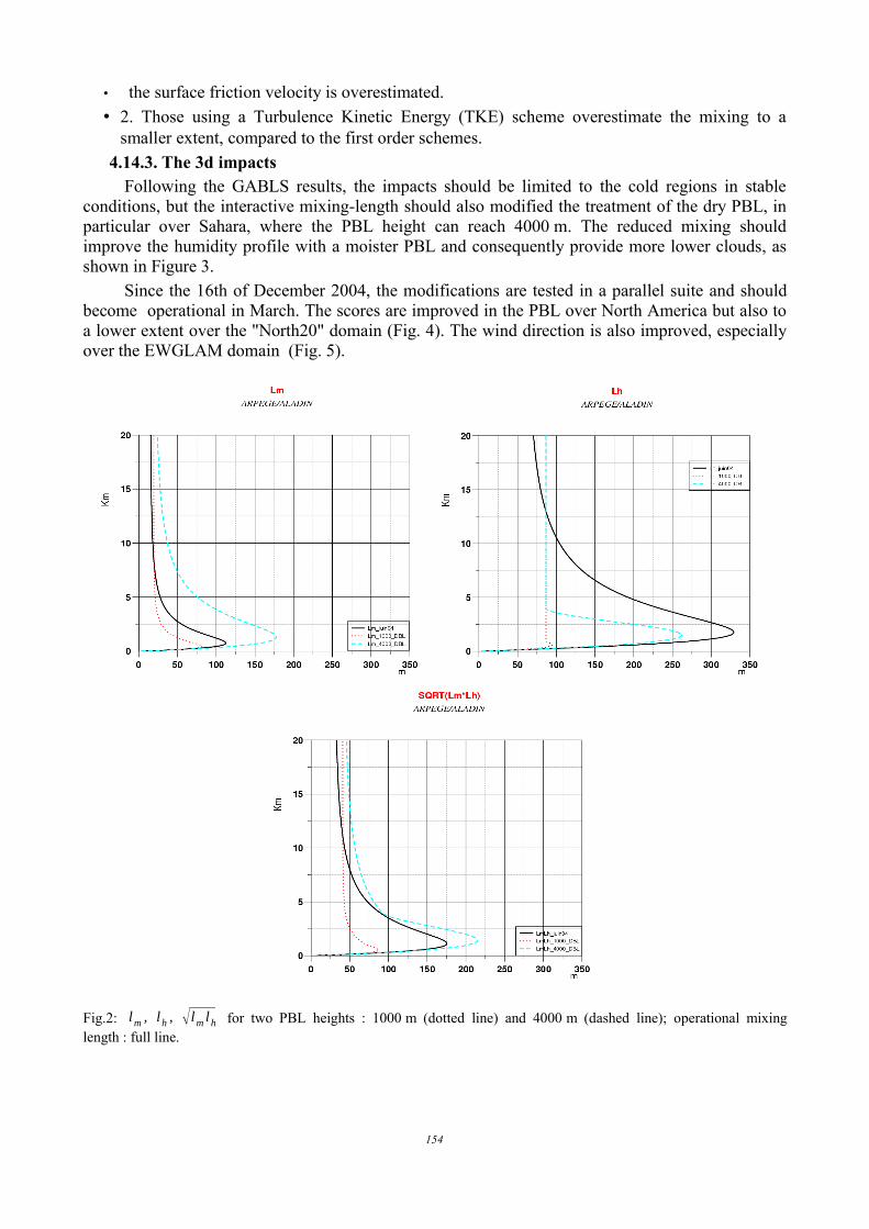
• the surface friction velocity is overestimated.• 2. Those using a Turbulence Kinetic Energy (TKE) scheme overestimate the mixing to a

smaller extent, compared to the first order schemes. 4.14.3. The 3d impacts

Following the GABLS results, the impacts should be limited to the cold regions in stableconditions, but the interactive mixing-length should also modified the treatment of the dry PBL, inparticular over Sahara, where the PBL height can reach 4000 m. The reduced mixing shouldimprove the humidity profile with a moister PBL and consequently provide more lower clouds, asshown in Figure 3.

Since the 16th of December 2004, the modifications are tested in a parallel suite and shouldbecome operational in March. The scores are improved in the PBL over North America but also toa lower extent over the "North20" domain (Fig. 4). The wind direction is also improved, especiallyover the EWGLAM domain (Fig. 5).

Fig.2: lm , lh , lm lh for two PBL heights : 1000 m (dotted line) and 4000 m (dashed line); operational mixinglength : full line.

154

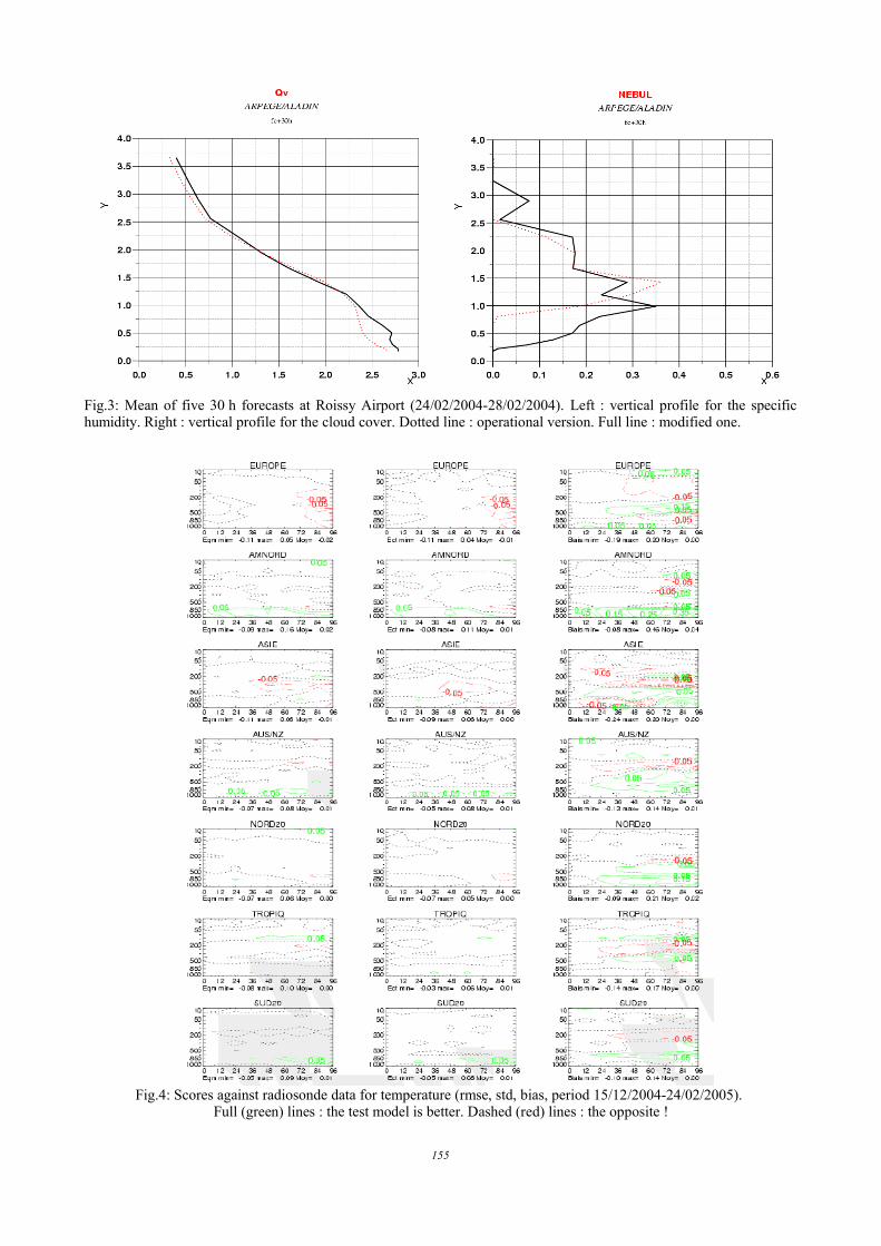
Fig.3: Mean of five 30 h forecasts at Roissy Airport (24/02/2004-28/02/2004). Left : vertical profile for the specifichumidity. Right : vertical profile for the cloud cover. Dotted line : operational version. Full line : modified one.

Fig.4: Scores against radiosonde data for temperature (rmse, std, bias, period 15/12/2004-24/02/2005). Full (green) lines : the test model is better. Dashed (red) lines : the opposite !

155

Fig.5: Score against SYNOP data (EWGLAM stations) for wind direction (rmse and bias, 15/12/2004-24/02/2005).Full (magenta) line : operational suite. Dashed(green) line: test suite

4.14.4. How to use it ?The modifications are on the cycle 28t3_op1 and when compared to the ALADIN export

version only a small modification in APLPAR is needed.In NAMPHY :

• add CGMIXLEN='TM' (the default is CGMIXLEN='Z')In NAMPHY0 :

• ALMAV=400. (operational scheme : ALMAV= 300.)• XMINLM=500. : minimum PBL height for the computation of lm/h

• XMAXLM=4000. : maximum PBL height for the computation of lm/h

• RICRLM=0.5 : critical Richardson number Ric used to determine the PBL height (default)• XBLM=8.5 : parameter to correct s : s = vsXBLM w ' ' vs /wm , wm is a function of the

friction velocity and the scale of the convective speed (the default is 6.5)• EDK=5. : new parameter used in the computation of Fm/h (operational scheme : EDK=1) • XKLM=0.6 : parameter to use the interactive PBL height for momentum

4.14.5. ReferencesCuxart, J., Holtslag, A., Beare, R., Bazile, E., , Beljaars, A., Cheng, A., Conangla, L., Ek, M., Freedman, F.,Hamdi, R., Kerstein, A., Kitagawa, H., Lenderink, G., Lewellen, D., Mailhot, J., Mauritsen, T., Perov, V.,Schayes, G., Steeneveld, G.-J., Svensson, G., Taylor, P., Weng, W., Wunsch, S., and Xu, K.-M., 2004 : Single-column model intercomparison for a stably stratified atmospheric boundary layer. Submitted to Bound.-LayerMeteor..Holtslag, A. A., 2003 : GABLS initiates intercomparison for stable boundary layer case. GEWEX News, 13:7--8.Kosovic, B. and Curry, J., 2000 : A large eddy simulation study of a quasi-steady, stably stratified atmosphericboundary layer. J. Atmos. Sci., 57, 1052--1068.Louis, J., Tiedtke, M., and Geleyn, J.-F., 1981 : A short history of the operational PBL-parameterization ofECMWF. In Workshop on Planetary Boundary Layer Parameterization, pages 59--79. [Available from ECMWF,Shinfield Park, Reading, RG29AX Berkshire, UK].Troen, I. and Mahrt, L., 1986 : A simple model of the atmosphere boundary layer; sensitivity to surfaceevaporation. Bound.-Layer Meteor., 37, 129—148.

156

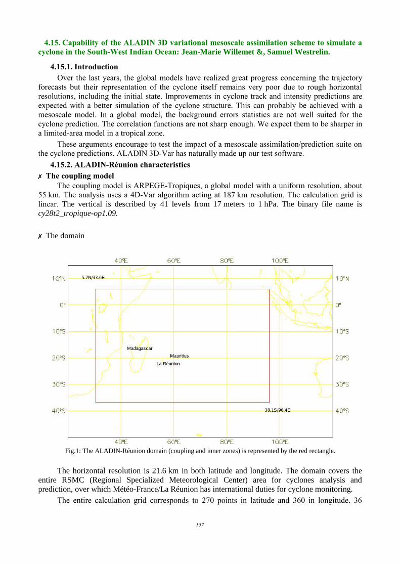
4.15. Capability of the ALADIN 3D variational mesoscale assimilation scheme to simulate acyclone in the South-West Indian Ocean: Jean-Marie Willemet &, Samuel Westrelin.

4.15.1. IntroductionOver the last years, the global models have realized great progress concerning the trajectory

forecasts but their representation of the cyclone itself remains very poor due to rough horizontalresolutions, including the initial state. Improvements in cyclone track and intensity predictions areexpected with a better simulation of the cyclone structure. This can probably be achieved with amesoscale model. In a global model, the background errors statistics are not well suited for thecyclone prediction. The correlation functions are not sharp enough. We expect them to be sharper ina limited-area model in a tropical zone.

These arguments encourage to test the impact of a mesoscale assimilation/prediction suite onthe cyclone predictions. ALADIN 3D-Var has naturally made up our test software. 4.15.2. ALADIN-Réunion characteristics✗ The coupling model

The coupling model is ARPEGE-Tropiques, a global model with a uniform resolution, about55 km. The analysis uses a 4D-Var algorithm acting at 187 km resolution. The calculation grid islinear. The vertical is described by 41 levels from 17 meters to 1 hPa. The binary file name iscy28t2_tropique-op1.09.

✗ The domain

Fig.1: The ALADIN-Réunion domain (coupling and inner zones) is represented by the red rectangle.

The horizontal resolution is 21.6 km in both latitude and longitude. The domain covers theentire RSMC (Regional Specialized Meteorological Center) area for cyclones analysis andprediction, over which Météo-France/La Réunion has international duties for cyclone monitoring.

The entire calculation grid corresponds to 270 points in latitude and 360 in longitude. 36

157

points in longitude and 27 in latitude are used for the extension zone necessary to get a biperiodicdomain; 8 points define the coupling zone both in latitude and longitude; the remaining pointsconstitute the inner area. The projection is the Mercator one. The vertical resolution is the same asin ARPEGE-Tropiques. The calculations grid is quadratic but it is planned to use a linear one in anear future.

✗ Background errors correlationsThey have been computed with the lagged-NMC method over the first quarter of 2004,

corresponding to warm season meteorological conditions. They should then better fit our cyclonicprediction aim. A rapid scan of these matrices showed that they contain some specific structuresprobably linked to the characteristics of the domain.

✗ The assimilation algorithmThe ALADIN 3D-Var available on OLIVE has been used with a 6 hours window.The assimilation is made at the same resolution as the forecast model. The observations file is

a simple extraction from the ARPEGE-Tropiques' one over our area.

4.15.3. Experiment description

✗ The case study : the cyclone BENTOThe forecasters have issued regular warnings on Bento between 20th and 30th of November

2004. Bento intensified very suddenly on the 22th. On the 23rd, it was an intense tropical cyclonewhich is rare at this period (Fig. 3). It moved slowly to the South at 10 km/h mean speed (Fig. 2).

ARPEGE-Tropiques forecasts were disappointing, particularly at the beginning of the cyclonelife (Fig. 4).

Fig.2: Observed BENTO track. Fig.3: Observed BENTO intensity.

158

Fig.4: ARPEGE-Tropiques 3-days forecasts every 12 hours on 00 and 12 UTC basis. The observed track is black.

✗ ALADIN configurationThe run cycle is al28t3_main.03. The assimilation of observations types 8 (cyclone bogus)

and 9 (QuickScat scatterometer winds) has been activated as in ARPEGE-Tropiques. To take intoaccount QuickScat winds, a new binary has been built which is used only for the observationsscreening. The forecast model has run on the 00h UTC basis up to 2 days.

The assimilation period extends from November the 19th at 06h UTC till the 30th at 00hUTC. It began one day before the first warning related to the system.

4.15.4. Results✗ Assimilation

- Assimilated observations More conventional observations and SATOB winds are assimilated by the ARPEGE-

Tropiques 4D-Var. The reason is intrinsic to the assimilation algorithm that takes into account thetemporal dimension. Several measures at the same place but at different times are used by 4D-Varwhen just one, associated to the time at the centre of the assimilation window, is used in 3D-Var.More aircrafts data are assimilated by ALADIN-Réunion; it has been noticed afterwards that theirthinning was looser than the ARPEGE-Tropiques' one. No difference appears for other observationtypes.

- Bento track and intensity analysis On average, the cyclone position (Fig. 6) is better forecasted by ALADIN-Réunion than by

ARPEGE-Tropiques, but the sample is very weak (10 forecasts). In both models the cycloneposition is analysed at the same position. The interesting feature is the decrease of the position-errorslope with range obtained in ALADIN-Réunion.

In the following paragraphs, the focus will be made on the cyclone structure.

159

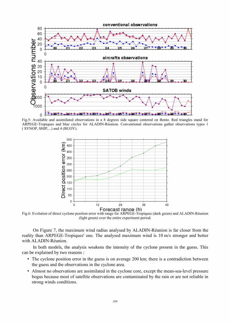
Fig.5: Available and assimilated observations in a 8 degrees side square centered on Bento. Red triangles stand forARPEGE-Tropiques and blue circles for ALADIN-Réunion. Conventional observations gather observations types 1( SYNOP, SHIP,...) and 4 (BUOY).

Fig.6: Evolution of direct cyclone position error with range for ARPEGE-Tropiques (dark green) and ALADIN-Réunion(light green) over the entire experiment period.

On Figure 7, the maximum wind radius analysed by ALADIN-Réunion is far closer from thereality than ARPEGE-Tropiques' one. The analysed maximum wind is 10 m/s stronger and betterwith ALADIN-Réunion.

In both models, the analysis weakens the intensity of the cyclone present in the guess. Thiscan be explained by two reasons :

• The cyclone position error in the guess is on average 200 km; there is a contradiction betweenthe guess and the observations in the cyclone area.

• Almost no observations are assimilated in the cyclone core, except the mean-sea-level pressurebogus because most of satellite observations are contaminated by the rain or are not reliable instrong winds conditions.

160

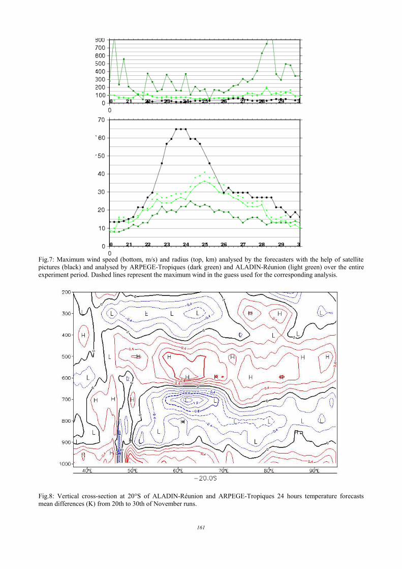
Fig.7: Maximum wind speed (bottom, m/s) and radius (top, km) analysed by the forecasters with the help of satellitepictures (black) and analysed by ARPEGE-Tropiques (dark green) and ALADIN-Réunion (light green) over the entireexperiment period. Dashed lines represent the maximum wind in the guess used for the corresponding analysis.

Fig.8: Vertical cross-section at 20°S of ALADIN-Réunion and ARPEGE-Tropiques 24 hours temperature forecastsmean differences (K) from 20th to 30th of November runs.

161

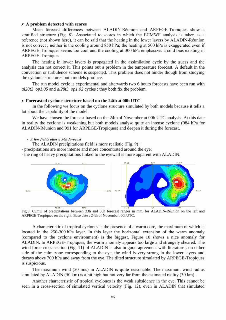
✗ A problem detected with scoresMean forecast differences between ALADIN-Réunion and ARPEGE-Tropiques show a

stratified structure (Fig. 8). Associated to scores in which the ECMWF analysis is taken as areference (not shown here), it can be said that the heating in the lower layers by ALADIN-Réunionis not correct ; neither is the cooling around 850 hPa; the heating at 500 hPa is exaggerated even ifARPEGE-Tropiques seems too cool and the cooling at 300 hPa emphasizes a cold bias existing inARPEGE-Tropiques.

The heating in lower layers is propagated in the assimilation cycle by the guess and theanalysis can not correct it. This points out a problem in the temperature forecast. A default in theconvection or turbulence scheme is suspected. This problem does not hinder though from studyingthe cyclonic structures both models produce.

The run model cycle is experimental and afterwards two 6 hours forecasts have been run withal28t2_op1.05 and al28t3_op1.02 cycles : they both fix the problem.

✗ Forecasted cyclone structure based on the 24th at 00h UTCIn the following we focus on the cyclone structure simulated by both models because it tells a

lot about the capability of the model.We have chosen the forecast based on the 24th of November at 00h UTC analysis. At this date

in reality the cyclone is weakening but both models analyse quite an intense cyclone (984 hPa forALADIN-Réunion and 991 for ARPEGE-Tropiques) and deepen it during the forecast.

- A few fields after a 36h forecast The ALADIN precipitations field is more realistic (Fig. 9) :

- precipitations are more intense and more concentrated around the eye;- the ring of heavy precipitations linked to the eyewall is more apparent with ALADIN.

Fig.9: Cumul of precipitations between 33h and 36h forecast ranges in mm, for ALADIN-Réunion on the left andARPEGE-Tropiques on the right. Base date : 24th of November, 00hUTC.

A characteristic of tropical cyclones is the presence of a warm core, the maximum of which islocated in the 250-300 hPa layer. In this layer the horizontal extension of the warm anomaly(compared to the cyclone environment) is the biggest. Figure 10 shows a nice anomaly forALADIN. In ARPEGE-Tropiques, the warm anomaly appears too large and strangely sheared. Thewind force cross-section (Fig. 11) of ALADIN is also in good agreement with literature : on eitherside of the calm zone corresponding to the eye, the wind is very strong in the lower layers anddecays above 700 hPa and away from the eye. The tilted structure simulated by ARPEGE-Tropiquesis suspicious.

The maximum wind (50 m/s) in ALADIN is quite reasonable. The maximum wind radiussimulated by ALADIN (50 km) is a bit high but not very far from the estimated reality (30 km).

Another characteristic of tropical cyclones is the weak subsidence in the eye. This cannot beseen in a cross-section of simulated vertical velocity (Fig. 12), even in ALADIN that simulated

162

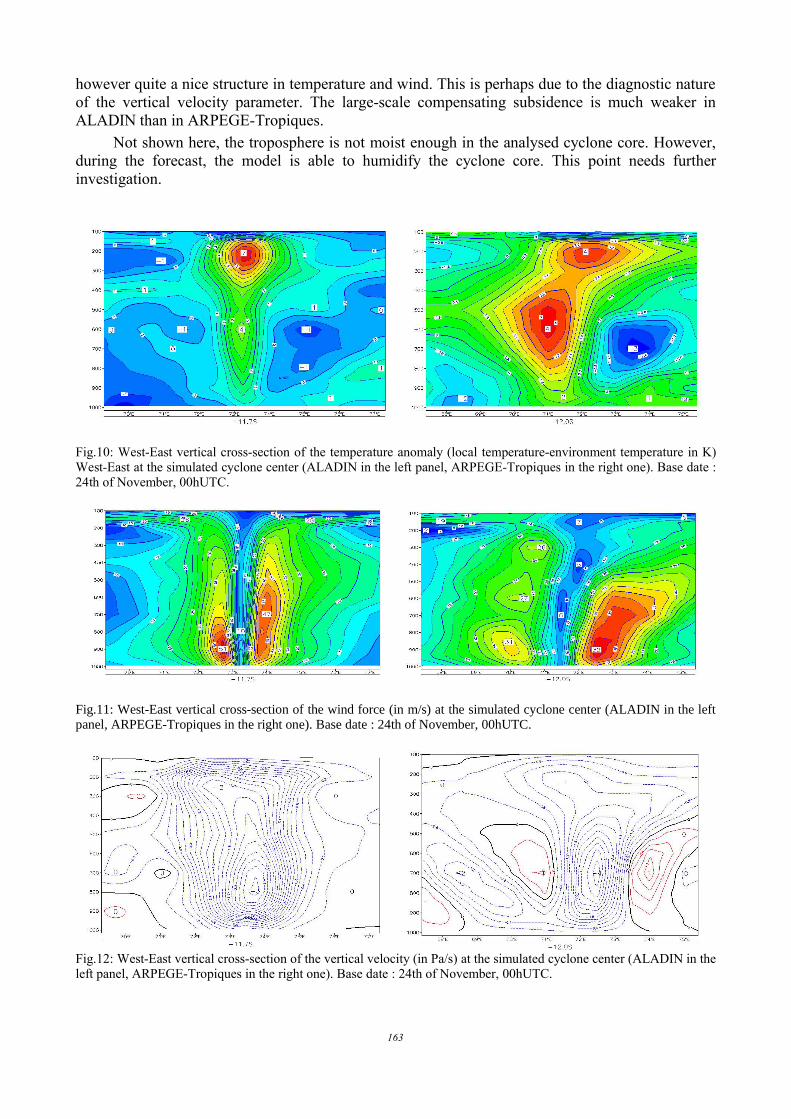
however quite a nice structure in temperature and wind. This is perhaps due to the diagnostic natureof the vertical velocity parameter. The large-scale compensating subsidence is much weaker inALADIN than in ARPEGE-Tropiques.

Not shown here, the troposphere is not moist enough in the analysed cyclone core. However,during the forecast, the model is able to humidify the cyclone core. This point needs furtherinvestigation.

Fig.10: West-East vertical cross-section of the temperature anomaly (local temperature-environment temperature in K)West-East at the simulated cyclone center (ALADIN in the left panel, ARPEGE-Tropiques in the right one). Base date :24th of November, 00hUTC.

Fig.11: West-East vertical cross-section of the wind force (in m/s) at the simulated cyclone center (ALADIN in the leftpanel, ARPEGE-Tropiques in the right one). Base date : 24th of November, 00hUTC.

Fig.12: West-East vertical cross-section of the vertical velocity (in Pa/s) at the simulated cyclone center (ALADIN in theleft panel, ARPEGE-Tropiques in the right one). Base date : 24th of November, 00hUTC.

163

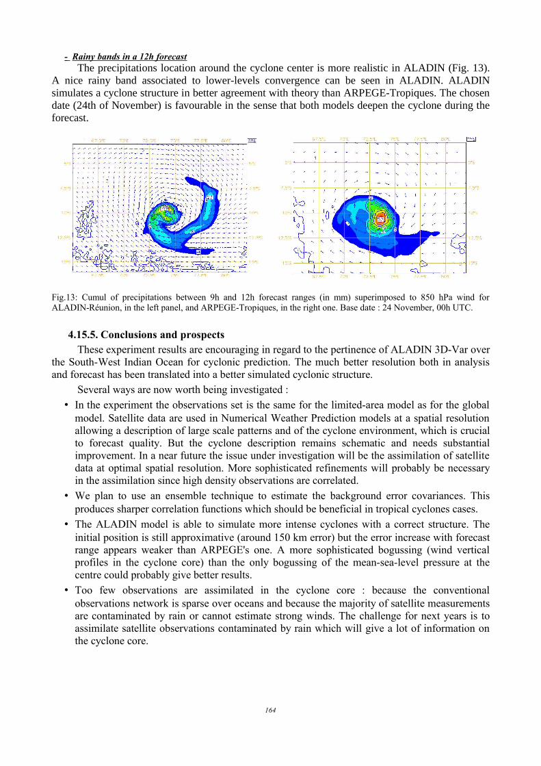
- Rainy bands in a 12h forecast The precipitations location around the cyclone center is more realistic in ALADIN (Fig. 13).

A nice rainy band associated to lower-levels convergence can be seen in ALADIN. ALADINsimulates a cyclone structure in better agreement with theory than ARPEGE-Tropiques. The chosendate (24th of November) is favourable in the sense that both models deepen the cyclone during theforecast.

Fig.13: Cumul of precipitations between 9h and 12h forecast ranges (in mm) superimposed to 850 hPa wind forALADIN-Réunion, in the left panel, and ARPEGE-Tropiques, in the right one. Base date : 24 November, 00h UTC.

4.15.5. Conclusions and prospectsThese experiment results are encouraging in regard to the pertinence of ALADIN 3D-Var over

the South-West Indian Ocean for cyclonic prediction. The much better resolution both in analysisand forecast has been translated into a better simulated cyclonic structure.

Several ways are now worth being investigated :• In the experiment the observations set is the same for the limited-area model as for the global

model. Satellite data are used in Numerical Weather Prediction models at a spatial resolutionallowing a description of large scale patterns and of the cyclone environment, which is crucialto forecast quality. But the cyclone description remains schematic and needs substantialimprovement. In a near future the issue under investigation will be the assimilation of satellitedata at optimal spatial resolution. More sophisticated refinements will probably be necessaryin the assimilation since high density observations are correlated.

• We plan to use an ensemble technique to estimate the background error covariances. Thisproduces sharper correlation functions which should be beneficial in tropical cyclones cases.

• The ALADIN model is able to simulate more intense cyclones with a correct structure. Theinitial position is still approximative (around 150 km error) but the error increase with forecastrange appears weaker than ARPEGE's one. A more sophisticated bogussing (wind verticalprofiles in the cyclone core) than the only bogussing of the mean-sea-level pressure at thecentre could probably give better results.

• Too few observations are assimilated in the cyclone core : because the conventionalobservations network is sparse over oceans and because the majority of satellite measurementsare contaminated by rain or cannot estimate strong winds. The challenge for next years is toassimilate satellite observations contaminated by rain which will give a lot of information onthe cyclone core.

164

4.16. GRIBEX introduction in FA files: D. Paradis and J. Clochard.

4.16.1. ContextMoore’s law, namely the doubling of the number of transistors on a chip every 18 months (or

the doubling of the computing power at fixed cost every 18 months), has been maintained for 40years, and still holds true today. However, in the face of this around 60 % annual increase of theCPU power, the memory access speed only grows by 7 % per year. Moreover, data storage and datainternational exchanges continuously raise, due to the resolution enhancement or the newproductions.

This trend motivated us to implement the use of the second order packing in the FA (FichierARPEGE) software: this feature is already available in GRIB edition 1 (GRIBEX) and allows tostore data on less bits than initially planned, without loss of accuracy. 4.16.2. Second order packing

Practically speaking, it may well be explained at encoding time. GRIB encoding of N gridpoint values on B bits leads to transform (in a linear fashion) original field values (generallyfloating-point) into the interval [0,2B-1], rounding them at the nearest integer values.

Ordinary ("simple") packing ends up processing at this stage, and packs the values obtainedinto a binary string of N*B bits.

The basic idea of second-order packing is to make extra processing, splitting the fullsequence of values into groups. For each group, an integer reference value is taken (such as theminimum value of the group), stored as descriptor ("first-order value"), and the positivedeviations from this reference value, called "second-order values", are then packed together,using just the bit number ("group width") sufficient for that.

The goal is clearly to reduce the overall size of data directly associated to field values,with a drawback of descriptors overhead. All the associated processing, performed on integer-typedata, is data conservative (lossless).

The "first-order" descriptors are stored on a bit number that uses the same place within GRIBas bit number for ordinary packing. There is also the need to document the group widths, andhow field is split into groups. To do so, there are three different methods available in WMOstandard: so-called row by row packing, constant width packing and a general method. All thesemethods (and sub-methods) do not change the data contents themselves at user level. ✗ Row by row packing.

The idea is to use coordinate lines as groups: for instance, latitude lines. The group splittingis "induced", and there is no need to document group boundaries (e.g. section 2 is sufficient).Computing of group widths is straightforward. Source coding may even be done without any workarray (but then leads to non optimal width of first-order values).

This method is in use at UKMO.✗ Constant width packing.

The idea is to save descriptors, but here on group widthes: there is a single group width,instead of one per group. Arbitrary group splitting is enabled; group boundaries are documentedby a secondary bit-map (one bit per effective grid point value, taking into account potentialprimary bit-map), with one bit set at each group starting point.✗ General WMO second-order packing.

In this case, all simplifications described in previous methods are relaxed. Secondary bit-map describes group boundaries as described above, and there is one group width per group.

Moreover, three extensions for the WMO standard have been coded to increase thecompression rate: general extended second-order packing, boustrophedonic ordering, and spatialdifferencing.

165

✗ General extended second-order packing.The first extension starts from a remark. The general WMO second-order packing exhibits

limitations for compression efficiency at 2 levels:-group widths are stored on 8 bits each (though 3 or 4 bits are generally sufficient);-secondary bit-map is a fixed but important overhead, and leads to "non-linear" source code

for decoding: group splitting may be described more economically (and decoded more simply)with group lengths, provided these lengths are encoded with an adapted width.

An extension may be coded, using an additional extended flag and three extra scalardescriptors (bit number of widths and lengths, pointer to group lengths), and re-allocating thesecondary bit-map area to store group lengths. This extension is a variant of general WMO second-order packing, and may use the same algorithm for group splitting.✗ Boustrophedonic ordering.

The second extension aims at giving a more continuous series of values for splitting. Theremay be large differences of values between 2 consecutive lines of coordinates, especially for non-global fields. To improve numerical continuity, lines of even rank (starting from the 2nd line, asspecified by scanning mode flags) may have their values reversed.

This may be described just by an appropriate extended flag, and coding is easy. It is a sub-method that may be applied to all second-order packing methods, but is disabled (at encodinglevel) for row by row packing, where it would have no interest (coordinate lines acting as groups).Such ordering is (in this context) fully handled internally within data section, and not reflected touser at data level.✗ Spatial differencing.

The basic idea of second-order packing methods is removal of local minima. But still, there isoften remaining point to point redundancy. This redundancy may be removed by preprocessingfield (integer) values just before second-order packing, using a spatial differencing scheme, (withorder N=1 to 3) that may be compared to approximation of a Nth-order derivative. That's signalprocessing, finding some echo with (analogic) derivative circuits in electronics.

This spatial differencing being not efficient for all fields, implementation has to determine apriori whether the feature is worthwhile to be used. This is achieved in relationship with splittingalgorithm, and so may only be selected sub-method with general extended second-order packing. 4.16.3. How to use it

Up to now, there were three possibilities to encode data with FA:Type 0 encoding: no packing is done, to preserve all the precision of the data (surface

geopotential for example);Type 1 encoding: GRIB version 0 is used only to code data in a packed form (data are

presented to GRIB in the integer form);Type 2 encoding: as type 1 encoding but with the storage (8 bytes) of the min and the max of

the data and with the use of all available bits.From now on (XR28T2), two other types are introduced:Type –1 encoding: no packing is done (the only difference with type 0 encoding is the

ordering of the spectral coefficients);Type 3 encoding: GRIB version 1 is used, with the possibility to make compression (second

order packing).First thing to do when using the type 3 or –1 encoding, is to keep the model ordering of

spectral fields: coefficients are ordered along |JM|=cte columns or, differently said, the zonal wavenumber, JM, is used as an outer loop index. The call to SPREORD routine before writing anhorizontal spectral field on a FA file or after reading one, is not yet useful (and must not be done!).

166

This is due to the fact that with the type 3 encoding, the FA software directly uses the GRIBEXcapability to pack Arpege spectral coefficients, which are supposed to be ordered as in model. Thisordering type has been kept to pack Aladin’s spectral coefficients with type 3 and the type –1encoding has been introduced to give the possibility to have only one spectral ordering type in a FAfile.

Secondly, the encoding type has to be specified to the FA software. There are two possibilitiesto do that:

. before opening the FA file(s), with a call to the FAGIOT routine,

. after you had opened the FA file, just call the FAGOTE routine.For these two calls, the KNGRIB argument has to be set to 3 (or –1 if no packing is required).

The number of bits used to pack the grid point values (KNBPDG) or the spectral coefficients(KNBCSP) and the non-packed sub-truncation (KSTRON) keep their meaning. You can reuse thepredefined values for these 3 variables by previously calling the FAVORI or FAVEUR routines.However, the two other arguments (KPUILA and KDMOPL) lose their sense in the type 3encoding.

Finally, you have to choose the second order packing options. The default in FA software, isto ask the selection of the best method between no-compression, row by row packing and thegeneral extended 2nd-order packing, to make a boustrophedonic ordering and a spatial differencingwith a dynamically estimated order. If these options have to be changed, the FAREGI or theFAREGU routines are available to modify the implicit tuning and the file specific tuningrespectively. You will then be able to activate/deactivate the boustrophedonic ordering, to modify oractivate/deactivate the spatial differencing, to activate/deactivate the general extended 2nd-orderpacking, to select constant width packing or general WMO second order packing, to ask GRIBEX toretain the most efficient packing method etc…

You can now write the horizontal fields with a FAIENC call!To summarize, here is the calling sequence you can use to encode ‘SURFTEMPERATURE’

with the type 3, in an already opened FA file:(…)integer irep, inumer; ingrib, inbcsp, inbpdg, istron, ipuila, idmoplreal*8 ztsurf(ngptot)logical llcosp(…)call faveur (irep, inumer, ingrib, inbcsp, inbpdg, istron, ipuila, idmopl)ingrib = 3call fagote (irep, inumer, ingrib, inbcsp, inbpdg, istron, ipuila, idmopl)llcosp = .false.call faienc (irep, inumer, ‘SURF’, 1, ‘TEMPERATURE’, ztsurf, llcosp)(…)To read an horizontal field, the use of the FACILE routine is identical whatever the encoding

type. Just remember that the ordering for the spectral fields is different between the types 0, 1 and 2and the types –1 and 3 (see above). 4.16.4. Some relevant features✗ ALADIN spectral fields

The only spectral coefficients that are accepted by the GRIB norm, are the spherical harmonicones (ARPEGE spectral fields, for example). To bypass this restriction, the FA software give to theALADIN spectral fields the appearance of a field on a quasi-regular latitude/longitude grid beforecalling GRIB code. Moreover, to better pack the spectral coefficients, the packing method for the

167

spherical harmonic coefficients is adapted and applied: first, all coefficients on the axes and in thesquare whose vertex have the coordinates (0,istron), (istron,0),(0,-istron) and (-istron,0), areextracted from the field and stored separately in the FA article with all the original precision (8bytes); then an optimal Laplacian exposant (“p”) is calculated to smooth the remaining spectrumwith the factor (jn**2 + jm**2)**p (“p” is stored in the FA article, as well as the non-packed sub-truncation “istron”); then the smoothed spectral field is given to GRIBEX to be packed as a gridpoints field, and being so able to take advantage of the second order packing.✗ ARPEGE spectral fields

As for the types 1 and 2 encoding, the type 3 encoding for an Arpege spectral field stores thespectral coefficients contained in the triangle defined by (jn<istron, where jn is the total wavenumber and istron the non-packed sub-truncation) separately in the FA article with all the originalaccuracy (8 bytes), the only difference being the presence of (istron+1)*(istron+2) non-packedcoefficients instead of (istron+1)**2, due to the difference in ordering.

Unlike the types 1 and 2 encoding, the type 3 encoding gives directly the whole originalARPEGE spectral field to GRIBEX and leaves it to transform the spectrum (smoothing by a factor(jn*(jn+1))**p, where jn is the total wave number and p the optimal laplacian exposant) beforepacking. The dynamical computation of the laplacian exponent (for ARPEGE and for ALADIN)makes all the pre-computed laplacian factors useless if only the type 3 encoding is used. For thetype 1 and 2 encodings, these pre-computed factors were actually stored in several arrays in FAsoftware and took up a lot space in memory when the maximal permitted truncation was high: thegoal was then to replace the CPU consumption by a memory consumption. Now, the aim haschanged and, with the constraint to only use the type 3 encoding, the memory need is greatly weakerand this advantage will become even more important when higher resolution will be used. A uniqueversion of the FA software will also allow very high resolution without needing too much memoryif the used resolution is actually crude.✗ GRIB auto documentation

The FA software uses the FA documentation articles to provide most of the informationnecessary to initialize the documentary sections of each GRIB message. However, the routineFAREGU can be used to specify another identification centre (KSEC1(2)=85 by default) or anothergenerating process identification number (KSEC1(3)=177 for ALADIN, 211 for ARPEGE forecastand 201 for ARPEGE analysis, by default). The routine FARPAR allows also to modify or to createa connection between an horizontal field name (prefix and suffix in FA) and its GRIB descriptors: 6integers which represent the version number of the parameters table (KSEC1(1)), the parameterindicator KSEC1(6), the type level indicator KSEC1(7), the level value KSEC1(8), the bottom ofthe layer in case of a layer or 0 otherwise (KSEC1(9)) and lastly a time range indicator KSEC1(18)(=0 except if the field is a min/max during a period (=2) or except if the field is an accumulation ina period (=4)). The basic connections are quite numerous (215 cases are taken into account in the setup of FA, see routine FAICOR) but the user can modify the connection of a field (prefix+suffix) orcreate new ones.

This auto documentation of the GRIB message and the respect for the GRIB norm allow todecode a FA file containing only type 3 encoded fields with other softwares such as the PBIOinterface of ECMWF : all GRIB messages (containing an horizontal field) can be completelyidentified except for GRIB messages containing an ALADIN spectral field (these fields aredisguised as grid points fields and the spectral coefficients have been transformed to be betterpacked).✗ Decimal factor

For each grid points field and each ALADIN spectral field, the FA software computes thedecimal factor which will optimize the bits use in the packing (for the type 3 encoding only). This

168

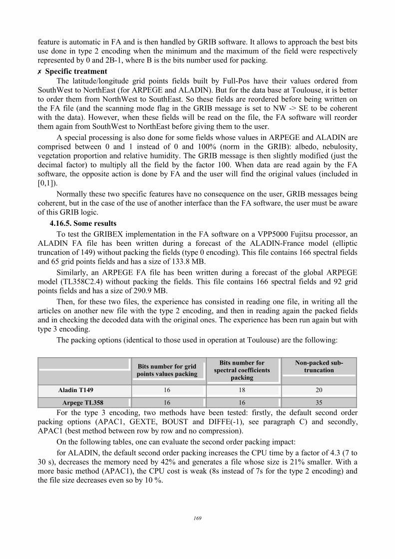
feature is automatic in FA and is then handled by GRIB software. It allows to approach the best bitsuse done in type 2 encoding when the minimum and the maximum of the field were respectivelyrepresented by 0 and 2B-1, where B is the bits number used for packing.✗ Specific treatment

The latitude/longitude grid points fields built by Full-Pos have their values ordered fromSouthWest to NorthEast (for ARPEGE and ALADIN). But for the data base at Toulouse, it is betterto order them from NorthWest to SouthEast. So these fields are reordered before being written onthe FA file (and the scanning mode flag in the GRIB message is set to NW -> SE to be coherentwith the data). However, when these fields will be read on the file, the FA software will reorderthem again from SouthWest to NorthEast before giving them to the user.

A special processing is also done for some fields whose values in ARPEGE and ALADIN arecomprised between 0 and 1 instead of 0 and 100% (norm in the GRIB): albedo, nebulosity,vegetation proportion and relative humidity. The GRIB message is then slightly modified (just thedecimal factor) to multiply all the field by the factor 100. When data are read again by the FAsoftware, the opposite action is done by FA and the user will find the original values (included in[0,1]).

Normally these two specific features have no consequence on the user, GRIB messages beingcoherent, but in the case of the use of another interface than the FA software, the user must be awareof this GRIB logic. 4.16.5. Some results

To test the GRIBEX implementation in the FA software on a VPP5000 Fujitsu processor, anALADIN FA file has been written during a forecast of the ALADIN-France model (elliptictruncation of 149) without packing the fields (type 0 encoding). This file contains 166 spectral fieldsand 65 grid points fields and has a size of 133.8 MB.

Similarly, an ARPEGE FA file has been written during a forecast of the global ARPEGEmodel (TL358C2.4) without packing the fields. This file contains 166 spectral fields and 92 gridpoints fields and has a size of 290.9 MB.

Then, for these two files, the experience has consisted in reading one file, in writing all thearticles on another new file with the type 2 encoding, and then in reading again the packed fieldsand in checking the decoded data with the original ones. The experience has been run again but withtype 3 encoding.

The packing options (identical to those used in operation at Toulouse) are the following:

Bits number for gridpoints values packing

Bits number forspectral coefficients

packing

Non-packed sub-truncation

Aladin T149 16 18 20

Arpege TL358 16 16 35For the type 3 encoding, two methods have been tested: firstly, the default second order

packing options (APAC1, GEXTE, BOUST and DIFFE(-1), see paragraph C) and secondly,APAC1 (best method between row by row and no compression).

On the following tables, one can evaluate the second order packing impact:for ALADIN, the default second order packing increases the CPU time by a factor of 4.3 (7 to

30 s), decreases the memory need by 42% and generates a file whose size is 21% smaller. With amore basic method (APAC1), the CPU cost is weak (8s instead of 7s for the type 2 encoding) andthe file size decreases even so by 10 %.

169

ALADIN T149 type of encoding 2 3

default options3

APAC1

Total user CPU time (s) 7 30 8

User vector CPU time (s) 2 14 1

System CPU time (s) 7 8 7

Memory (MB) 384 224 224

File size (MB) 38.1 30.2 34.5

for ARPEGE, the default second order packing increases the CPU time by a factor of 2.8 (12to 33 s), decreases the memory need by 42% and generates a file whose size is 22% smaller. Withthe APAC1 method, the CPU cost is, once again, negligible but the file size does not go downgreatly: only 5%.

ARPEGE T358 type of encoding 2 3

default options3

APAC1

Total user CPU time (s) 12 33 13

User vector CPU time (s) 1 12 1

System CPU time (s) 15 14 15

Memory (MB) 384 224 224

File size (MB) 74.9 58.7 71.2

To detail the behaviour of the second order packing (with the defaults options), one can see itswork on each field of the two files. The first figure shows the length of each field (spectral ones andthen grid points ones) for the ALADIN FA file. In this case, the second order packing is also appliedto the spectral coefficients but the gain is weaker than with grid points values (the point to pointredundancy is actually less important).

170

A similar figure is proposed for the ARPEGE fields. No second order packing is then appliedto the spectral coefficients and the corresponding articles are a little bit larger than with the type 2encoding, due to the more documented GRIB sections (which allow the GRIB to be decodedindependently from the FA software).

Comparison of the FA article lengths between type 2 and type 3 encoding for Arpege TL358

0

10000

20000

30000

40000

50000

1 166

166 spectral fields and 92 grid points fields

Leng

th o

f the

pac

ked

field

(wor

d)

type 2 encodingtype 3 encoding

Finally, the precision of the encoding has been compared for the type 2 and 3 encodings.

Except for the ALADIN spectral coefficients which lose less precision, all other fields seem to be alittle less accurate with the type 3 encoding. It is well explained by the better use of the bits donewith the type 2 encoding, despite the decimal factor optimization in the type 3 encoding. Anyway,the overall impact on the quality of the fields have to be evaluated with an e-suite and a comparisonbased on meteorological criteria instead of statistical ones.

171

5. PUBLICATIONS

5.1. Bénard P., R. Laprise, J. Vivoda & P. Smolíková: Stability of Leapfrog Constant-Coefficients Semi-Implicit Schemes for the Fully Elastic System of Euler Equations: Flat-Terrain Case. Monthly Weather Review: Vol. 132, No. 5, pp. 1306–1318.http://www.ametsoc.org

ABSTRACTThe stability of semi-implicit schemes for the hydrostatic primitive equations system has been studied extensively over the

past 20 yr, since this temporal scheme and this system represented a standard for NWP. However, with the increase of computationalpower, the relaxation of the hydrostatic approximation through the use of nonhydrostatic fully elastic systems is now emerging forfuture NWP as an attractive solution valid at any scale. In this context, several models employing the so-called Euler equationstogether with a constant- coefficients semi-implicit time discretization have already been developed, but no solid justification for thesuitability of this algorithmic combination has been presented so far, especially from the point of view of robustness.

The aim of this paper is to investigate the response of this system/scheme in terms of stability in presence of explicitly treatedresidual terms, as it inevitably occurs in the reality of NWP. This study is restricted to the impact of thermal and baric residual terms(metric residual terms linked to the orography are not considered here). It is shown that, conversely to what occurs with hydrostaticprimitive equations, the choice of the prognostic variables used to solve the system in time is of primary importance for therobustness with Euler equations. For an optimal choice of prognostic variables, unconditionally stable schemes can be obtained (withrespect to the length of the time step), but only for a smaller range of reference states than in the case of hydrostatic primitiveequations. This study also indicates that (i) vertical coordinates based on geometrical height and on mass behave similarly in terms ofstability for the problems examined here, and (ii) hybrid coordinates induce an intrinsic instability, the practical importance of whichis, however, not completely elucidated in the theoretical context of this paper.

5.2. Termonia Piet: Monitoring the Coupling-Update Frequency of a Limited-Area Modelby Means of a Recursive Digital Filter. Monthly Weather Review: Vol. 132, No. 8, pp. 2130–2141. http://www.ametsoc.org

ABSTRACTIn operational applications lateral-boundary coupling data are provided to one-way nested limited-area models with time

intervals of more than an order of magnitude larger than the time step of the coupled model. In practice, these fixed coupling-updatefrequencies are established by common-sense guesswork and by technical restrictions rather than by rigorous methods. As a result,situation-dependent failures are never completely excluded when coupling data enter the domain more rapidly than can be sampledby the a priori fixed frequency. To avoid misinterpreting such failures, the data transfer between the coupling and the coupled modelshould be monitored.

The present paper approaches this as a problem of undersampling. It investigates how the coupling-update frequency can bemonitored by using a digital recursive filter in the coupling model. A response function for such a filter is derived. Itsimplementation in a NWP model is discussed and some extensive tests are presented. A possible application is discussed in whichthis monitoring is used for assessing the data transfer to the coupled model and additionally for adapting the coupling updates to theactual meteorological content of the coupling-model output.

5.3. Bénard P.: On the Use of a Wider Class of Linear Systems for the Design of Constant-Coefficients Semi-Implicit Time Schemes in NWP. Monthly Weather Review: Vol. 132, No. 5,pp. 1319–1324. http://www.ametsoc.org

ABSTRACTThe linearisation of the meteorological equations around a specified reference state, usually applied in NWP to define the

linear system of constant-coefficients semi-implicit schemes, is outlined as an unnecessarily restrictive approach that may bedetrimental in terms of stability. It is shown theoretically that an increased robustness can sometimes be obtained by choosing thereference linear system in a wider set of possibilities. The potential benefits of this new approach are illustrated in two simpleexamples. The advantage in robustness is not obtained at the price of an increased error or complexity.

5.4. Sadiki W. and C. Fischer: A posteriori validation applied to the 3D-VAR ARPEGE andALADIN data assimilations system. Tellus 57A pp.21-34.

http://www.blackwellpublishing.com/ABSTRACTIn this paper we present results from the application of a posteriori diagnostics on existing data assimilation systems. The

systems of interest are the global data assimilation Arpège 3D-VAR of Météo-France, and the limited-area 3D-VAR analysis of

172

ALADIN. First, we discuss how the diagnostics can be ported from theory to practical applications, using aggregates of analysisinformation over time. We then compare the behaviour of the diagnostics in the two different data assimilation systems, with a focuson the properties of the background and observational error variances. Secondly, the a posteriori validation is used for the off-linetuning of two scalar error parameters in the ALADIN 3D-VAR. The tuning provides error variances that better fit the statistics of theinnovation vector, without loss of quality in the analyses. Finally, the link of this approach with ensemble-based techniques is made.Especially, we propose to couple the a posteriori diagnostics directly with the usual output of ensemble samples, which could bedone at no extra cost. If the results are then used to tune error parameters, then an on-line adaptive assimilation system, based on aposteriori considerations, is obtained.

5.5. Stefanescu S. and L. Berre: Ensemble dispersion spectra and the estimation of errorstatistics for a limited area model analysis. WGNE.

173

CONTENTS1.EDITORIAL.................................................................................................................................... 3 1.1.EVENTS .....................................................................................................................................3 1.1.1.26th EWGLAM and 11th SRNWP meetings......................................................................................3 1.1.2.9th Assembly of ALADIN Partners.................................................................................................... 3 1.1.3.TCWGPDI workshop.......................................................................................................................... 3 1.1.4.HIRLAM-ALADIN mini-workshop on convection and cloud processes...........................................4 1.1.5.Other workshops..................................................................................................................................4 1.1.6.Other events.........................................................................................................................................4 1.2.ANNOUNCEMENTS................................................................................................................. 4 1.2.1. HIRLAM All Staff Meeting............................................................................................................... 4 1.2.2.2nd SRNWP workshop on "Short-Range Ensemble Prediction Systems"......................................... 5 1.2.3.4th WMO international symposium on "Assimilation of Observations in Meteorology andOceanography"....................................................................................................................................................5 1.2.4.ICAM-MAP meeting........................................................................................................................... 5 1.2.5.LM Users seminar............................................................................................................................... 5 1.2.6.3rd SRNWP workshop on "Statistical and Dynamical Adaptation"...................................................5 1.2.7.15th ALADIN workshop "QUO VADIS, ALADIN ?".......................................................................6 1.2.8.And next ............................................................................................................................................. 6 1.3.ALADIN 2................................................................................................................................... 6 1.3.1.Introduction......................................................................................................................................... 6 1.3.2.A closer ALADIN-HIRLAM cooperation.......................................................................................... 7 1.3.3.STORMNET........................................................................................................................................9 1.3.4.Coordination......................................................................................................................................10 1.3.5.The misfortunes of the ALARO-10 sub-project, arguments around the physics-dynamicsinterface, ...........................................................................................................................................................10 1.3.6.Communication problems, obviously................................................................................................11 1.3.7.Fourth medium-term research plan................................................................................................... 12 1.3.8.Support.............................................................................................................................................. 12 1.4.GOSSIP..................................................................................................................................... 132.OPERATIONS...............................................................................................................................15 2.1.An overview of operational ALADIN applications January 2005............................................ 15 2.1.1.Model characteristics........................................................................................................................ 15 2.1.2.Practical implementation...................................................................................................................16 2.1.3.Porting new versions......................................................................................................................... 17 2.1.4.Conclusion.........................................................................................................................................17 2.2.Changes in the Operational Version of ARPEGE..................................................................... 17 2.2.1.October, 19th: Observations & Physics & Assimilation changes.....................................................17 2.2.2.Winter new version: modification of the mixing lengths of the turbulence scheme........................ 18 2.2.3.Towards a new ARPEGE schedule: objective and intermediate steps............................................. 18 2.3.AUSTRIA (more details [email protected]).............................................................21 2.4.BELGIUM (more details [email protected])................................................................... 21 2.5.BULGARIA (more details [email protected])....................................................... 21 2.6.CROATIA (more details [email protected],[email protected]) ...................................... 21

174

2.6.1.Introduction....................................................................................................................................... 21 2.6.2.Test of new Czech setup....................................................................................................................21 2.7.CZECH REPUBLIC (more details [email protected] ) ........................................................ 22 2.7.1.Operations......................................................................................................................................... 22 2.7.2.Parallel Suites & Maintenance.......................................................................................................... 27 2.8.FRANCE (more details [email protected]) .......................................................................... 28 2.9.HUNGARY (more details [email protected]) ......................................................................... 28 2.10.MOROCCO (more details [email protected]) .............................................................28 2.11.POLAND (more details [email protected]) ................................................................... 28 2.12.PORTUGAL (more details [email protected]).............................................................28 2.13.ROMANIA (more details [email protected])......................................................29 2.14.SLOVAKIA (more details [email protected]) ........................................................... 29 2.14.1.Summary..........................................................................................................................................29 2.14.2.The new operational ALADIN setup.............................................................................................. 29 2.14.3.Local R&D work and Future plans................................................................................................. 32 2.15.SLOVENIA (more details [email protected] )..............................................................34 2.16.TUNISIA (more details [email protected])...............................................................................34 2.17.RSEARCH & DEVELOPMENTS AUSTRIA .......................................................................35 2.17.1.INCA–A high-resolution analysis and nowcasting system based on ALADIN forecasts ............. 35 2.17.2.Quantitative evaluation of the orographic precipitation problem in ALADIN...............................37 2.17.3.Stratus prediction.............................................................................................................................38 2.17.4.Evaluation of mesoscale precipitation forecasts in the Southern Alpine area ...............................38 2.17.5.Verification of dynamically downscaled wind............................................................................... 39 2.17.6.Development of a LAM ensemble prediction system using ALADIN........................................... 39 2.18.BELGIUM .............................................................................................................................. 39 2.18.1.Stability and accuracy of the physics-dynamics interface.............................................................. 39 2.18.2.Monitoring the coupling-update frequency.....................................................................................39 2.18.3.2 m temperature forecasts ................................................................................................................40 2.18.4."Wavelet Jb"....................................................................................................................................40 2.18.5.Adaptations to ALADIN of the Lopez micro-physical package.....................................................40 2.18.6.Gravity wave drag........................................................................................................................... 40 2.18.7.Physics-Dynamics Interface............................................................................................................ 41 2.19.BULGARIA ............................................................................................................................41 2.19.1.New Integration Domain for ALADIN-BG.................................................................................... 41 2.19.2.Porting cycle 28T3.......................................................................................................................... 42 2.19.3.A lot of work in Toulouse !............................................................................................................. 42 2.20.CROATIA............................................................................................................................... 42 2.21.CZECH REPUBLIC ...............................................................................................................42 2.21.1.ALADIN/MFSTEP configuration...................................................................................................42 2.21.2.Bottom boundary condition.............................................................................................................42 2.21.3.Tests of SLHD and gravity wave drag in the ALPIA framework ..................................................42 2.21.4.SLHD developments....................................................................................................................... 42 2.22.FRANCE ................................................................................................................................ 43 2.22.1.Introduction..................................................................................................................................... 43

175

2.22.2.Source code maintenance................................................................................................................ 43 2.22.3.Dynamics, geometry and coupling.................................................................................................. 47 2.22.4.Physics & Co................................................................................................................................... 50 2.22.5.Data assimilation............................................................................................................................. 52 2.23.HUNGARY............................................................................................................................. 55 2.24.MOROCCO: PROGRESS REPORT ON NUMERICAL WEATHER PREDICTION..........55 2.24.1.A brief summary of research development and main operational changes.................................... 55 2.24.2.Research and Development in data assimilation and numerical forecasting..................................56 2.24.3.Research and Development results for application of NWP products............................................57 2.24.4.Outstanding research and development activities related to improvement of the operationalsystem................................................................................................................................................................58 2.24.5.REFERENCE.................................................................................................................................. 59 2.25.POLAND................................................................................................................................. 61 2.26.PORTUGAL............................................................................................................................61 2.27.ROMANIA ............................................................................................................................. 61 2.27.1.The implementation of cycle 28T3 on SUN E4500 and Linux cluster platforms (Cornel Soci)... 61 2.27.2.Dynamical adaptation of the wind using the ALADIN NH (Steluta Alexandru)........................... 62 2.27.3.The flash flood event of 28th of August 2004 (Doina Banciu and Cornel Soci)........................... 62 2.27.4.The common ALADIN verification project (Simona Stefanescu)................................................. 62 2.27.5.First test on EPS ALADIN-Romania (Mihaela Caian) ..................................................................62 2.27.6.Verification of spectral coupling method on daily basis (Raluca Radu)........................................ 63 2.28.SLOVAKIA.............................................................................................................................67 2.29.SLOVENIA ............................................................................................................................ 67 2.29.1.Verification project......................................................................................................................... 67 2.29.2.Testing of Latent Heat Nudging in ALADIN Model...................................................................... 67 2.29.3.Probability forecast of temperature with quantile regression method............................................ 67 2.29.4.High-resolution wind climatology...................................................................................................67 2.30.TUNISIA ................................................................................................................................ 68 2.30.1.Changes in coupling files resolution as a solution to the transfer problem.................................... 68 2.30.2.Other events.....................................................................................................................................68

3.ALADIN PhD Studies................................................................................................................... 69 3.1.Incrementality deficiency in ARPEGE 4d-var assimilation scheme: Radi Ajjaji: ................... 69 3.2.Scientific strategy for the implementation of a 3D-Var data assimilation scheme for a double-nested limited-area model: Steluta Alexandru....................................................................................69 3.3.Estimation and study of forecast error covariances using an ensemble method in a global NWPmodel: Margarida Belo-Pereira.......................................................................................................... 69 3.4.Further Improvement of a Simplified 2D Variational Soil Water Analysis: K. Bergaoui. ...... 69 3.5.Evaluation of assimilation cycles in a mesoscale limited area model: Vincent Guidard. ........ 69 3.5.1.Formalism: a very brief reminder......................................................................................................69 3.5.2.Evaluation over a 15-day period....................................................................................................... 69 3.6.Interaction between physical processes: cloud life cycle, cloud transient states: Jean-MarcelPiriou.................................................................................................................................................. 73 3.7.Extensive study of the coupling problem for a high-resolution limited-area model: RalucaRadu....................................................................................................................................................73 3.8.A posteriori verification of analysis and assimilation algorithms and study of the statistical

176

properties of the adjoint solutions: Wafaa Sadiki...............................................................................73 3.9.Study of the relationship between turbulent fluxes in deeply stable PBL situations andcyclogenetic activity: André Simon. ..................................................................................................73 3.10.Systematic qualitative evaluation of high-resolution non-hydrostatic model: KlausStaldbacher......................................................................................................................................... 74 3.11.The modelling of the forecast error covariances for a 3D-Var data assimilation in anatmospheric limited-area model: Simona Stefanescu. .......................................................................74 3.12..Use of IASI/AIRS observations over land: Małgorzata Szczech-Gajewska.......................... 74 3.13.Application of the Predictor-Corrector Method to non-hydrostatic dynamics: J. Vivoda. .....74 3.14.A survey on well-posed and transparent lateral boundary conditions (LBCs) in spectrallimited-area models: Fabrice Voitus...................................................................................................754.PAPERS and ARTICLES.............................................................................................................76 4.1.Some informal news from the AROME project: F. Bouttier, G. Hello, S. Malardel, Y. Seity,with help from many others................................................................................................................76 4.1.1.Objectives..........................................................................................................................................76 4.1.2.Using the Méso-NH physics..............................................................................................................76 4.1.3.The state of the prototype..................................................................................................................77 4.1.4.The remaining work.......................................................................................................................... 79 4.1.5.Computational cost issues................................................................................................................. 81 4.1.6.Assimilation, predictability and coupling......................................................................................... 81 4.1.7.Conclusion.........................................................................................................................................82 4.1.8.Basic references on the Méso-NH physics and fine-scale assimilation:...........................................83 4.2.Use of geostationnary SEVIRI radiances in ALADIN 3D-Var: Montmerle Thibaut..............83 4.2.1.Introduction....................................................................................................................................... 83 4.2.2.Presentation of the product................................................................................................................84 4.2.3.Pre-processing of the data................................................................................................................. 84 4.2.4.Impact on analyses............................................................................................................................ 86 4.2.5.Impact on forecast............................................................................................................................. 88 4.2.6.Conclusions and future work.............................................................................................................93 4.2.7.References:........................................................................................................................................ 93 4.3.Case of extreme wind occurrence at high Tatras on 19th November 2004: Vivoda J. & SimonA. ....................................................................................................................................................... 94 4.3.1.Summary ...........................................................................................................................................94 4.3.2.Operational prediction of ALADIN/SHMI....................................................................................... 94 4.3.3.High resolution prediction of ALADIN............................................................................................ 95 4.3.4.References......................................................................................................................................... 96 4.4.High-resolution dynamical adaptation of the wind forecast using the non-hydrostatic versionof the ALADIN model: Alexandru S..................................................................................................96 4.4.1.Introduction....................................................................................................................................... 96 4.4.2.The experimental results................................................................................................................... 97 4.4.3.Conclusions..................................................................................................................................... 100 4.4.4.References....................................................................................................................................... 100 4.5.Pre-operational testing of a 3D-VAR assimilation in ALADIN-FRANCE: Fischer C., Th.Montmerle & L. Berre...................................................................................................................... 100 4.5.1.Initial choices.................................................................................................................................. 100

177

4.5.2.Impact of B matrix and statistical behaviour of the assimilation...................................................100 4.5.3.Case studies..................................................................................................................................... 101 4.5.4.Conclusions and outlook................................................................................................................. 104 4.5.5.Bibliography.................................................................................................................................... 105 4.6.Latest results of the LAMEPS experiments: Hágel E............................................................. 105 4.6.1.Motivation....................................................................................................................................... 105 4.6.2.Experiments.....................................................................................................................................105 4.6.3.Experiments with different target times..........................................................................................107 4.6.4.Experiments with combining different sets of singular vectors......................................................111 4.6.5.Preliminary conclusions.................................................................................................................. 112 4.6.6.Future plans..................................................................................................................................... 112 4.6.7.References....................................................................................................................................... 113 4.7.The HIRALD setup: B. H. Sass, K. Lindberg & B. S. Andersen. .......................................... 113 4.7.1.Introduction..................................................................................................................................... 113 4.7.2.Evolution of the HIRALD setup..................................................................................................... 114 4.7.3.First experiments............................................................................................................................. 115 4.7.4.Future work..................................................................................................................................... 116 4.8.Spline interpolation in semi-Lagrangian advection scheme of ALADIN/ARPEGE/IFS: VáňaFilip. .................................................................................................................................................118 4.8.1.Introduction..................................................................................................................................... 118 4.8.2.Spline interpolation in ALADIN/ARPEGE/IFS............................................................................. 119 4.8.3.Performance of the splines.............................................................................................................. 121 4.8.4.Conclusion.......................................................................................................................................123 4.8.5.References....................................................................................................................................... 123 4.9.Impact of observations and tuning of observational error statistics: Chapnik Bernard. .........125 4.9.1.Introduction..................................................................................................................................... 125 4.9.2.Theory..............................................................................................................................................125 4.9.3.Practical Computation of Trace (HK)............................................................................................. 126 4.9.4.The tuning of variances................................................................................................................... 127 4.9.5.Properties of the method................................................................................................................. 128 4.9.6.Impact of the tuning of the variance................................................................................................129 4.9.7.Conclusion.......................................................................................................................................129 4.9.8.References....................................................................................................................................... 129 4.10.Adaptations to ALADIN of the Lopez micro-physical package: Gérard Luc....................... 131 4.10.1.Introduction................................................................................................................................... 131 4.10.2.Original scheme.............................................................................................................................131 4.10.3.Scheme adaptations....................................................................................................................... 132 4.10.4.The precipitation routine............................................................................................................... 133 4.10.5.Conclusions................................................................................................................................... 133 4.10.6.References..................................................................................................................................... 133 4.11.VARPACK– A diagnostic Tool, based on the 3DVar/ALADIN surface scheme: Auger L &Taseva L........................................................................................................................................... 134 4.11.1.Introduction................................................................................................................................... 134 4.11.2.Section I – Basic features of Diagpack and Varpack ................................................................... 134 4.11.3.Section II – Experiments with Varpack........................................................................................ 138

178

4.11.4.Impact of the observations for altitude stations............................................................................ 142 4.11.5.Section III. Conclusions and intents for the future work.............................................................. 142 4.11.6.Acknowledgements ...................................................................................................................... 143 4.11.7.References..................................................................................................................................... 143 4.12.An update on the 2002 Gard flood simulation with the ALARO-10 prototype in 2004: Acomparison between ALADIN, Méso-NH, ALARO-10 and AROME: Hello Gwen...................... 143 4.12.1.Summary .......................................................................................................................................143 4.12.2.Characteristics of the different runs used .....................................................................................144 4.12.3.Results........................................................................................................................................... 144 4.12.4.Conclusion.....................................................................................................................................150 4.13.The "how?" and "why?" of the discretized governing equations in the proposed new physics-dynamics interface: Catry B............................................................................................................ 150 4.14.Interactive mixing length and modifications of the exchange coefficient for the stable case: E.Bazile, G. Beffrey, M. Joly and H. Marzouki...................................................................................152 4.14.1.Introduction................................................................................................................................... 152 4.14.2.The modifications..........................................................................................................................152 4.14.3.The 3d impacts.............................................................................................................................. 154 4.14.4.How to use it ?...............................................................................................................................156 4.14.5.References..................................................................................................................................... 156 4.15.Capability of the ALADIN 3D variational mesoscale assimilation scheme to simulate acyclone in the South-West Indian Ocean: Jean-Marie Willemet &, Samuel Westrelin................... 157 4.15.1.Introduction................................................................................................................................... 157 4.15.2.ALADIN-Réunion characteristics.................................................................................................157 4.15.3.Experiment description................................................................................................................. 158 4.15.4.Results........................................................................................................................................... 159 4.15.5.Conclusions and prospects............................................................................................................ 164 4.16.GRIBEX introduction in FA files: D. Paradis and J. Clochard............................................. 165 4.16.1.Context.......................................................................................................................................... 165 4.16.2.Second order packing.................................................................................................................... 165 4.16.3.How to use it..................................................................................................................................166 4.16.4.Some relevant features.................................................................................................................. 167 4.16.5.Some results...................................................................................................................................169

5.PUBLICATIONS.........................................................................................................................172 5.1.Bénard P., R. Laprise, J. Vivoda & P. Smolíková: Stability of Leapfrog Constant-CoefficientsSemi-Implicit Schemes for the Fully Elastic System of Euler Equations: Flat-Terrain Case. MonthlyWeather Review: Vol. 132, No. 5, pp. 1306–1318. http://www.ametsoc.org .................................172 5.2.Termonia Piet: Monitoring the Coupling-Update Frequency of a Limited-Area Model byMeans of a Recursive Digital Filter. Monthly Weather Review: Vol. 132, No. 8, pp. 2130–2141.http://www.ametsoc.org ...................................................................................................................172 5.3.Bénard P.: On the Use of a Wider Class of Linear Systems for the Design of Constant-Coefficients Semi-Implicit Time Schemes in NWP. Monthly Weather Review: Vol. 132, No. 5, pp.1319–1324. http://www.ametsoc.org ...............................................................................................172 5.4.Sadiki W. and C. Fischer: A posteriori validation applied to the 3D-VAR ARPEGE andALADIN data assimilations system. Tellus 57A pp.21-34.............................................................. 172 5.5.Stefanescu S. and L. Berre: Ensemble dispersion spectra and the estimation of error statisticsfor a limited area model analysis. WGNE........................................................................................ 173

179

ALADIN NEWSLETTER 27 - umr-cnrm.fr

Documents

Transcript of ALADIN NEWSLETTER 27 - umr-cnrm.fr