
A.(k,p) - Durham e-Theses - Durham University
192
• • •
Transcript of A.(k,p) - Durham e-Theses - Durham University

Durham E-Theses
A non-perturbative study of the infra-red behaviour of
QCD
Brown, Nicholas
How to cite:
Brown, Nicholas (1989) A non-perturbative study of the infra-red behaviour of QCD, Durham theses,Durham University. Available at Durham E-Theses Online: http://etheses.dur.ac.uk/6575/
Use policy
The full-text may be used and/or reproduced, and given to third parties in any format or medium, without prior permission orcharge, for personal research or study, educational, or not-for-pro�t purposes provided that:
• a full bibliographic reference is made to the original source
• a link is made to the metadata record in Durham E-Theses
• the full-text is not changed in any way
The full-text must not be sold in any format or medium without the formal permission of the copyright holders.
Please consult the full Durham E-Theses policy for further details.
Academic Support O�ce, Durham University, University O�ce, Old Elvet, Durham DH1 3HPe-mail: [email protected] Tel: +44 0191 334 6107
http://etheses.dur.ac.uk
A NON-PERTURBATIVE STUDY
OF THE INFRA-RED BEHAVIOUR
OF QCD
Nicholas Brown
Department of Physics
University of Durham
The copyright of this thesis rests with the author.
No quotation from it should be published without
his prior written consent and information derived
from it should be acknowledged.
A thesis submitted to the University of Durham
for the Degree of Doctor of Philosophy
August 19.88
- 6 J u l 1989
There are more things in heaven and earth, Horatio, than are dreamt
of in your philosophy.
Hamlet, Act I, Scene V.
. ABSTRACT
The non-perturbative behaviour of the non-Abelian gauge theory of
strong interactions, namely Q(;D, is investigated using the Schwinger-Dyson
equations. Using an approximation based on solving the Slavnov-Taylor iden
tities, we derive a closed integral equation for the full gluon propagator. \Ve
numerically solve this equation, finding a consistent solution which is as sin
gular as 1/p4 as the momentum p2 - 0, whilst at large momenta the gluon
propagates like a free particle.
This infra-red behaviour can be seen as a signal for the confinement of
quarks and gluons, implying, for example, that the Wilson loop operator behaves
an 'area law'.
\Ve then derive an equation for the full massless quark propagator. Us
ing our solution for the gluon, we find the quark propagator to be suppressed at
low momentum, to such an extent that the physical particle pole is removed, and
free quarks cannot propagate. This is just what we might expect of a confining
theory.
The inclusion of quarks means we must study their dynamical effects
via closed fermion loops in the gluon propagator equation. This couples the
two equations together. We solve the two equations simultaneously, finding that
the previous infra-red behaviour still holds. As we introduce more flavours of
fermions, however, the infra-red enhancement of the gluon propagator is dimin
ished, and this in turn means that the quark propagator is less suppressed. This
exhibits the dynamical importance of quarks.
These physically realistic results demonstrate the importance and va
lidity of the Schwinger-Dyson equations as a valuable tool for investigating the
non-perturbative features of gauge theories.
ACKNOWLEDGEMENTS
This thesis owes its existence to many people. First and foremost of
these is my supervisor Mike Pennington, who has helped above and beyond
the call of duty. He has been teacher, collaborator, banker, foster parent, car
salesman, reprimander (usually justified), p.r. man, employment adviser, and
most of all a friend. He has shown every confidence in me (not always justified),
and is to him that any complaints should be addressed. Thanks Mike, and may
the SERC triple your salary!
I must also thank Alan Martin and Kaoru Hagiwara, who both showed
great patience in helping me take my first tentative steps.
Five months of my time were spent at Brookhaven National Laboratory,
New York, U.S.A. It is a pleasure to thank Bill Marciano and the rest of the
theory group there for their hospitality. Whilst admitting that I learnt much
scientifically, I would like to take this opportunity to warn young single people
who are even remotely sociable against staying there. It is appropriate to take
a quote from Jeremy Bernstein's autobiographical 'The life it brings':
'It was (and is) a wonderful place scientifically, but for me, after my
year in France, it caused a dras.tic culture shock'. (My italics).
Special thanks to Patti Pennington for her kindness and hospitality, and for the
best eating house on Long Island.
Then we come to those electronic machines, which would have remained
an enigma to me, were it not for Stuart Grayson, who showed me how to switch
them on, and to Mike Whalley, who is ever ready to answer the most stupid of
questions.
Particular mention must go to the fellow occupants of room 303: Simon
Webb, Yanos Michopoulos, Mohammed Nobary and Mohammed Hussein. They
not only had to suffer my continuous chatter, but also had the same addiction
to caffeine as myself. What can I say? 5-a-side, home brew, Greek holidays,

siestas, naughty postcards, the Vic. on a friday night. How could one have
survived three years in Durham "'"ithout them? May the Mykonos philosophy
live (or is it sleep) on.
Special commendation goes to those in the group who rarely discuss
physics: Nigel Glover (mentioned in dispatches for outstanding cynicism), An
thony Allan, Tony Peacock, Martin Carter, Jenny Nicholls, Ahmed Bawa, David
Pentney, James Stirling, Dominic Walsh and Michael Wade. No disrespect of
course to those who did occasionally talk shop, after all we shouldn't forget
our purpose in life: Peter Collins, Chris Maxwell and not least, Peter Harri
man. On the subject of physicists, I must also thank Ed Witten for his letter of
encouragement.
A cosmologist or two for luck: Laurence Jones who must also be men
tioned for much hospitality when the beer had taken effect, and for taking pity
on the homeless; also Duncan Hale-Sutton. Without the sterling efforts of these
two young gentlemen the publicans of Durham would be much the poorer.
These last three years would lie heavier on me than othen..,ise were it
not for the gentler sex, who made the place look (and occasionally feel) prettier.
In alphabetical order: Ann, Ann, Clare, Coral, Kate, Mandy, Margaret, Sally,
Sara and Sue. Special mention to Vicky Augustynek for forcing various and
collected Italian dishes down my throat. Most of all though, thanks and much
love to Helen.
Last, and by no means least, I must thank my parents for their support
and love. If I have not always done as they would have wished, they have never
criticised.
Princeton University Department of Physics: Joseph Henry Laboratories Jadwin Hall Post Office Box 708 Princeton, New Jersey 08544
8.-eA ~4</-14 ' 1./~ ~ / 'A/}
~/
fi-- td../ ~ ..»~-r::U?0; v
Telephone: 609 452-4400 Tc:lc:x: 499-3512
To Mum, Dad, and Helen

DECLARATION
I declare that no material in this thesis has previously been submitted
for a degree at this or any other university.
The research described in chapters three~ four~ five and six has been
carried out in collaboration with Dr. M.R. Pennington and has been published
as follows:
(i) 'Preludes to Confinement: Infra-red Properties of the Gluon Propagator
in the Landau gauge'
N. Brown and M.R. Pennington, Phys. Lett. 106B (1988) 133
(ii) 'Studies of Confinement: How Quarks and Gluons Propagate'
N. Brown and M.R. Pennington, Brookhaven preprint BNL-41101, to
be published in Phys. Rev. D (1988)
The copyright of this thesis rests with the author. No quotation from it
should be published without prior written consent and any information derived
from it should be acknowledged.
Other published work by the author:
(i) 'Scalar Electron and Zino Production on and Beyond the Z Resonance
in e+ e- Annihilation'
A.R. Allan~ N. Brown and A.D. Martin, Z. Phys. C31 (1986) 479
(ii) 'Polarization Amplitudes and Predictions for e+ e- -+ n-y'
N. Brown, K. Hagiwara and A.D. Martin, Nucl. Phys. B288 {1987)
783

(iii) 'Parisi Mulitijet Shape Variables in e+ e- Annihilation in terms of Par
tonic Energy-Momentum Fractions'
N. Brown, Y. Michopoulos and M.R. Pennington, J. Phys. G 14 (1988)
519
(iv) 'An Improved Presentation of a Novel Perturbative Scheme in Field
Theory'
N. Brown, Phys. Rev. D38 (1988) 723
(v) 'Perturbative QCD Algorithms for Transverse Momentum Distributions
in e+ e- Annihilation'
Y. Michopoulos, N. Brown and M.R. Pennington, J. Phys. G 14 (1988)
1027
TABLE OF CONTENTS
CHAPTER ONE STRONG INTERACTIONS
1.1 Introduction
1.2 Historical Background
1.3 Local Gauge Invariance
1.4 Perturbative QCD
1.5 Confinement
CHAPTER TWO THE SCHWINGER-DYSON EQUATIONS
2.1 Path Integrals and F\mctional Methods in Field Theory
2.2 The Schwinger-Dyson Equations for Scalar Field Theory
2.3 Fermions and Path Integrals
2.4 The Schwinger-Dyson Equations for QCD
2.5 The Slavnov-Taylor /VVard-Takahashi Identities
2.6 The Perturbative Gluon and Quark Propagators
CHAPTER THREE THE GLUON EQUATION
3.1 Derivation of the Equation for Q(p)
3.2 The Gluon Loop
3.3 Renormalisation
3.4 Consistent Asymptotic Behaviour of 9 R(P)
3.5 Technical Details
3.6 The Solution
CHAPTER FOUR THE MANDELSTAM APPROXIMATION
4.1 Introduction
1
2
11
15
20
24
30
33
34
41
50
54
57
62
67
70
81
84
4.2
4.3
4.4
4.5
The Calculation and Renormalisation
The Solution
How Good is the Mandelstam Approximation?
Confinement and a 1/ p4 Gluon Propagator
CHAPTER FIVE THE FERMION EQUATION
5.1
5.2
5.3
5.4
Introduction
The Ward Identity and the Equation for :F(p)
Renormalisation
The Solution for :FR(P)
CHAPTER SIX QUARK LOOPS
6.1
6.2
6.3
Introduction
The Quark Loop Diagram
The Gluon Equation with Quarks
85
90
94
97
110
111
115
123
128
130
135
CHAPTER SEVEN A NON-PERTURBATIVE STUDY OF QCD
7.1 Propagation of Quarks and Gluons 149
7.2 Ultraviolet Problems 151
7.3 Infra-red Problems 156
7.4 Approximations and Improvements 161
7.5 Comments on the Solutions 164
APPENDIX A INTEGRALS 167
REFERENCES 177

1.1 Introduction
Chapter One Strong Interactions
CHAPTER ONE
STRONG INTERACTIONS
The modern study of particles and their interactions has provided us
with the great successes of non-Abelian gauge theories, which in their second
quantised form provide us Vvith an extremely accurate description of the weak
and electromagnetic forces. These two interactions are seen to be different man
ifestations of a more fundamental 'electroweak' force. This was experimentally
confirmed by the discovery of the W and Z bosons[l.l], which along with the
photon constitute the carriers of this force. It also appears that another non
Abelian gauge theory, that of Quantum Chromodynamics (QCD), may well
provide us with a dynamical theory of the strong nuclear force. Unfortunately,
despite many succesful predictions at collider energies, we do not yet under
stand the most important manifestation of this strong interaction, namely the
plethora of low energy bound states we call hadrons; their masses, lifetimes,
decay modes and interactions. Nevertheless, a great many theoretical physicists
accept this 'standard model' of relatively low energy physics as proven, and cast
their research efforts towards 'loftier' goals.
The most important of these is to try and understand how the eligible
bachelor of general relativity can be married to the unwilling bride of quantum
theory. It is hoped that the offspring of such a match would be a full quantum
description of gravity, the attainment of which has been one of the outstanding
aims of physics for over fifty years. Unfortunately it is unlikely that we shall
find any experimental evidence to guide us below energies of the Planck mass
("" 1019 Ge V), a scale totally inaccessible to the earth bound scientist for the
forseeable future. Indeed, experiment has yet to give us any real clues about
physics beyond the standard model, despite the belief of most physicists that
1

Chapter One Strong Interactions
there is much more to learn.
In the absence of experimental clues, much research is guided less by
physical intuition and more by a desire for mathematical elegance, an avenue
which has not always proven the most fruitful. The most recent craze is for
'superstring' theories, which are held to promise the unification of all known
(and unknown) forces. Here the fundamental objects are not particles, but
one dimensional 'strings', living in some higher dimensional space-time. As
a growing band of physicists fiock to the superstring banner, it is worthwhile
to consider that we have still to understand the existence of many 'everyday'
particles such as the proton and neutron, the building blocks of nearly all matter
in the universe!
This study is an examination of the proposed theory of strong interac
tions, namely QCD, at the low energies where hadrons dominate. H QCD is the
theory of strong interactions then there are some fundamental questions which
must be answered. Here we describe a framework which may well provide these
answers and we make some first steps towards them, obtaining results which
qualitatively at least, are physically realistic, and bode well for future studies.
We shall, however, try to highlight various shortcomings and problems which
will hopefully be addressed in future studies.
1.2 Historical Background
The earliest manifestation of strong interactions is now known to be
the production of a-rays in the nuclear decays of uranium. The radiation from
uranium was first observed by Becquerel in 1896. At the time however, the
nucleus was yet to be discovered and these so called 'Becquerel rays' remained
unexplained.
It was 1911 before Rutherford proposed the nucleur model of the atom
to explain the large angle scattering of a-rays off a gold foil target as observed by
2

Chapter One Strong Interactions
Geiger and Marsden. Subsequent experiments confirmed Rutherford's scattering
formula and the atomic nucleus came into existence.
In many ways Rutherford .was fortunate that the energy of his a-rays
(,...., 5 MeV) was too low to penetrate the Coulomb barrier of the relatively heavy
nuclei, such as gold, used in the target. After the first world war the experi
ment was repeated but this time with light nuclei, particularly Hydrogen, in the
target, for which the coulomb repulsion was less. For the first time induced nu
clear reactions were observed[l.2] as massive deviations from the electromagnetic
coulomb repulsion, the first signal of a new force.
Despite the success of the nuclear model, the problem remained of
atomic mass and it was not until 1930 that Bothe and Bekke observed a new
penetrating form of radiation. Chadwick was then able to show that this was
due to a new, electrically neutral particle with the same mass as the proton.
With this new particle, the neutron (n), and the already discovered electron
(e) and proton (p), the family of subatomic particles seemed complete. The
atom was held to be a small central nucleus consisting of protons and neutrons,
around which the electrons orbited.
The question remained as to how the nucleus was held together against
the electrostatic Coulomb repulsion of the protons. Experiment showed that
the n- n, p- p, and n- p nuclear forces we~e similar in strength, leading to
the conclusion that the nuclear force was independent of the electrical charge
of the particle involved. This was made into a more sophisticated statement by
considering the neutron and proton as two different aspects of one particle, the
nucleon (N), similar in concept to the two different spin states of any spin-! '
particle. More exactly, the nucleon was a doublet of isotopic spin or isospin,
I= !· The proton was assigned Ia = +! and the neutron 13 = -!, where Ia
is the third component of the isospin vector. The nuclear forces were invariant
under the isospin rotations of the group SU(2).
3

Chapter One Strong Interactions
On a more dynamical level, Yukawa proposed that this force would be
carried by a particle called the pi-meson or pion ( 1r ), by analogy ·with how the
photon carried the electromagnetic force. Because of the short range of the
nuclear forces, this pion would have to be massive, of the order of 100 Mev. A
particle of this mass was indeed observed in cosmic rays and naturally identified
as the pion. Unfortunately it had all the wrong properties and was later realised
to be a more massive copy of the electron, which became known as the muon
(J.l ). The pion itself was discovered just after the second world war, and had all
the properties expected.
These early advances went hand in hand vdth the development of quan
tum theory, and particularly quantum field theory, in which particles were cre
ated and annihilated in interactions. Unfortunately quantum field theories are
plagued mth infinities in any calculations beyond the lowest order in pertur
bation theory, the only known consistent method for performing calculations.
These occur in momentum (loop) integrals which are divergent at large, or 'ul
traviolet' momenta. One of the major theoretical successes of the thirties and ·
forties was to show that for quantum electrodynamics (QED) the theory of
electromagnetism, that these infinities could be absorbed into infinite renormal
isations of the fields, masses and coupling constants. Any quantity was then
finite when expressed in terms of these renormalised quantities. This program
of renormalisation has allowed calculations to be performed in QED in which
we can obtain the finest agreement known between theory and experiment.
At the same time people tried to develop a quantum field theory of the
strong (and weak) nuclear forces. Perturbation theory expresses quantities as
a power series in the coupling constant. For QED the relevant quantity is the
fine structure constant a ~ 1i7 • Since this .is a small number, we might expect
the first few terms of such a series to give accurate answers. The same quantity
for strong interactions was estimated to be of the order of 10. A power series in
4

Chapter One Strong Interactions
this was likely to be meaningless, without addressing the problem of finding a
theory which could be made finite by renormalisation. Perhaps the situation is
best summed up in a conversation between Dirac and Feynman when they first
met in 1961[1.3):
F.
D.
F.
D.
I am Feynman.
I am Dirac. (Silence.)
It must be wonderful to be the discoverer of that equation.
That was a long time ago. (Pause.)
D. What are you working on?
F. Mesons.
D. Are you trying to find an equation for them?
F. . It is very hard.
D. One must try.
In 1947 the situation was further complicated by the discovery of new
particles in cosmic rays by Rochester and Butler[1.4]. These were called V
particles because of the tracks they made in the bubble chambers. Soon new
particles were being copiously produced in accelerators. It was noticed that
these new particles were always produced in pairs, and this led to the idea
of 'associated production', or conservation of a new quantum number known
as strangeness (S). The known particles, the proton, neutron and pion were
assigned zero strangeness, i.e S=O. So, for example, in the reaction
1r+ + n --. J(+ +A
the new particles ](+ and A were assigned strangeness S= + 1 and S= -1
respectively, and strangeness is seen to be conserved in this allowed reaction.
This concept also helped to explain the relatively long lifetimes of these strange
particles ( ...... 10-9 s compared to the usual strong interaction scale of ..... 10-23s).
5

Chapter One Strong Interactions
Since strong interactions conserved strangeness, these particles could only decay
via the weak nuclear force which was seen to violate strangeness conservation,
but was very much weaker than the strong force, leading to long lifetimes.
The way forward was by an extension of the isospin SU(2) symmetry.
The three pions ( 7r+, 7!"0 , 71"-) fitted into this symmetry as an I= 1 triplet of
isospin. With the discovery of strange particles, similar assignments were looked
for. Gell-Mann and others[1.5] realised that the particles could be fitted into
representations of the larger group SU(3), which contained the isospin SU(2) as
a subgroup. SU(3) has eight generators compared to three for SU(2). Some of
these SU(3) multiplet assignments are shown in fig. 1.1.
If this SU(3) symmetry were exact, then all particles in the same multi-
plet would have the same mass. Deviations from this were larger than those seen
within isospin multiplets. By assuming that isospin is an exact symmetry, and
that the mass term breaking the SU(3) symmetry transforms like the eighth
generator of SU(3) it was possible to derive a formula relating the masses of
the different particles in the multiplets. This is the famous Gell-Mann- Okubo
mass formula for the octet, which states that
with MN = 940 MeV, M=. = 1320 MeV, MA = 1115 MeV and ME = 1190 MeV,
this formula is seen to hold to a good approximation. More importantly, at the
time the n- was missing from the decuplet in fig. 1.1. Gell-Mann was able
to predict its mass of 1680 MeV and its electric charge. When in 1964 such a
particle was discovered with the correct mass and charge at Brookhaven, SU(3)
symmetry was in!
Despite its apparent simplicity, it seemed that nature did not want to
use the simplest representations of SU(3), namely a triplet 3, and its conjugate
representation 3. It is possible to build up all the higher representations by
6

Chapter One Strong Interaction.s
a) b)
n ,---___,1---...... P
s-
c)
n-
Fig. 1.1: SU(3) particle multiplets: a) JP = o- meson octet, b)JP =!+baryon
octet, c)JP =!+baryon decuplet. Horizontal axis denotes 13 , vertical
axis denotes Hypercharge Y = S + B, where B is baryon number.
7

Chapter One Strong Interactions
taking tensor products of these fundamental representations. For example we
have:
3 ® 3 ® 3 = 10 Ef7 8 Ef7 8 Ef7 1
Those hadrons with integer spin, known as mesons, e.g. the pions,
appeared in multiplets from the first of these decompositions, those with half
integer spin, known as the baryons, from the second. It was as though there were
three fundamental particles with spin-! in the 3 representation called quarks
(q). The mesons appeared to be made from qq pairs, and the baryons from qqq
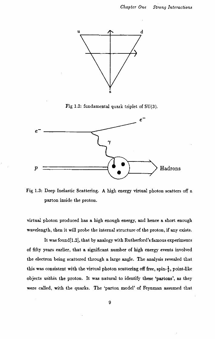
combinations. This quark triplet is shown in fig 1.2. It consists of an up (u)
quark of charge+~ and a down (d) and strange (s) quark both of charge -k· If the masses of the up and down quarks were the same, with the strange quark
heavier, then this would give rise to the correct mass formula which was seen to
hold to a good approximation. By assigning Is = +t, -!, 0 and S= 0, 0,-1 to
the u,d,s quarks respectively, the correct quantum numbers for the hadrons were
obtained. The u,d,s labels have become known as different ':flavours' of quarks.
It should be stressed that at this stage quarks were purely mathematical
objects, and their fractional electric charge in partiCular made it difficult for
them to be thought of as real particles.
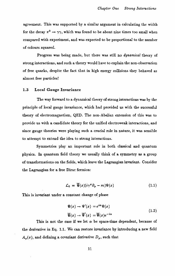
The situation changed dramatically in what has become known as the
Deep Inelastic Scattering experiments performed at SLAC during the sixties.
Here high energy electrons were scattered onto protons. The latter broke up to
create a shower of hadrons. As far as we know an electron is a truly fundamental
particle, It therefore survives the impact and can be detected in the final state
to 'tag' the collision. The process is depicted diagramatically in fig. 1.3. If the
8
Chapter One Strong Interactions
u d
s
Fig 1.2: fundamental quark triplet of SU(3).
e
e
p Hadrons
Fig 1.3: Deep Inelastic Scattering. A high energy virtual photon scatters off a
parton inside the proton.
virtual photon produced has a high enough energy, and hence a short enough
wavelength, then it will probe the internal structure of the proton, if any exists.
It was found[L2], that by analogy with Rutherford's famous experiments
of fifty years earlier, that a significant number of high energy events involved
the electron being scattered through a large angle. The analysis revealed that
this was consistent with the virtual photon scattering off free, spin-!, point..,like
objects within the proton. It was natural to identify these 'partons', as they
were called, with the quarks. The 'parton model' of Feynman assumed that
9

Chapter One Strong Interactions
these quarks were essentially free inside the proton, and that they interacted
instantaneously with the incident photon. It. was on a much larger time scale
that the subsequent break-up and hadronisation of the proton into the final state
particles occured. This model had much success in phenomenological studies of
hadrons. Quarks had arrived as real particles! Despite these successes, problems
still remained:
(i) Why were free quarks not observed in nature, and only qq, qqq combinations
seen.
(ii) Quarks must have spin-! to explain the observed hadrons. The~++ with
third component of spin Sa = +l must therefore be made up from three up
quarks all with Sa = +! and therefore have a symmetric wave function with
respect to interchange of any two of these identical quarks. This was a violation
of Fermi-Dirac statistics.
The most satisfactory solution to this second problem is to suppose
that the quarks have an additional quantum number, which we shall call colour, . and that the colour wave function is antisymmetric with respect to interchange
of quarks. Thus it is postulated that all observable hadrons axe singlets with
respect to the colour degree of freedom.
How many colours are there? This can be answered by experiment. For
example the ratio
R = u(e+e- -+ hadrons) u(e+e--+ J.l+J.l-)
is naively expected to be constant and equal to the sum of the squares of the
quark charges. For three flavours (and later four and five) this ratio was found
to be a factor of three too small when compared with experiment. By proposing
three colours, each flavour of quark is counted three times and we can obtain
10
Chapter One Strong Interactions
agreement. This was supported by a similar argument in calculating the width
for the decay 1r0 --+"'("'(,which was found to be about nine times too small when
compared with experiment, and was expected to be proportional to the number
of colours squared.
Progress was being made, but there was still no dynamical theory of
strong interactions, and such a theory would have to explain the non-observation
of free quarks, despite the fact that in high energy collisions they behaved as
almost free particles!
1.3 Local Gauge Invariance
The way forward to a dynamical theory of strong interactions was by the
principle of local gauge invariance, which had provided us with the successful
theory of electromagnet~sm, QED. The non-Abelian extension of this was to
provide us with a candidate theory for the unified electroweak interactions, and
since gauge theories were playing such a crucial role in nature, it was sensible
to attempt to extend the idea to strong interactions.
Symmetries play an important role in both classical and quantum
physics. In quantum field theory we usually think of a symmetry as a group
of transformations on the fields, which leave the Lagrangian invariant. Consider
the Lagrangian for a free Dirac fermion:
{1.1)
This is invariant under a constant change of phase
- _, - . w(z)--+ \l1 (z) = \ll(z)e-•a-
(1.2)
This is not the case if we let a be space-time dependent, because of
the derivative in Eq. 1.1. We can restore invariance by introducing a new field
A"(z), and defining a covariant derivative D", such that
11
Chapter One Strong Interactions
where g is a free parameter.
Consider the new Lagrangian:
(1.4)
This is invariant under the phase transformations in Eq. 1.1 with a now a( x),
a function of space-time x, if we let the field A 11 transform as:
(1.5)
As yet the new gauge field A 11 has no kinetic term, and so we add the
simplest term quadratic in A 11 (x) and invariant under the transformation of Eq.
1.5, to obtain the well known Lagrangian:
(1.6)
where
(1. 7)
This is the Lagrangian for QED, where we identify A"(x) as the photon field.
Its interaction with the electron field \ll(x) is uniquely defined by demanding
invariance under local phase, or gauge transformations. Composition of these
phase transformations forms the Abelian group U(l ).
We expect the quark field to have three components because of the three
degrees of colour:
,y, _- ( tPred ) '!t.' tPblue
tPgreen
12

Chapter One Strong Interactions
where we use the labels red,blue and green to denote the three colours.
Thus our free Lagrangian for one flavour of quark will be:
Co = \l1(x)(ip- m)\l1(x) (1.8)
but where the \l1(x) are three component quantities.
This is invariant under the transformations of the larger non-Abelian
group SU(3) (not to be confused with the flavour SU(3) invariance above):
(1.9)
where the eight quantities A4 /2 are the Gell-Mann 3 x 3 matrices which generate
the group SU(3). The 84 are eight phase parameters. The A4 satisfy the well
known commutation relations:
[_xa _xbl 2 ' 2
(1.10)
where the /abc are called the structure constants of the group
Following the same procedure as that for QED, we would like to de
rive a Lagrangian which is invariant when the 84 become the space-time de
pendent functions 84 (x). This time we have to introduce eight gauge fields
A~(x ), one for each generator of the group. Introducing the matrix function
U(x) = eiB"(z)'A"/2 , we define the covariant derivative in a similar way to be-
fore:
{1.11)
where it is to be stressed that D 11 is a 3 x 3 matrix, and we will write A 11 (x) for
the matrix A~(x ).X 4 /2.
We can obtain invariance under local SU(3) transformations provided
A 11 ( x) transforms as:
13
Chapter One Strong Interactions
(1.12)
The covariant derivative has the transformation property:
(1.13)
And so the quantity F;, = - i / g ( D I', D, J transforms in the same way.
Explicit calculation yields:
(1.14)
Using the commutation relations in Eq. 1.10, and writing the matrix F~'" as
F;, ..\a /2 we obtain:
(1.15)
This is the non Abelian extension of Eq. 1.7. Thus our gauge invariant La-
grangian will now read:
(1.16)
This is the classical Lagrangian from which the quantum field theory
known as QCD is obtained. In other words QCD is the theory of gauged SU(3)
colour transformations, specifying how the coloured quarks interact with the
non-Abelian gauge fields we call gluons (g). Unlike QED it should be noted
that the gluons themselves carry the colour charge, and so can interact with
other gluons, a feature of essential importance.
Finally it should be mentioned that gauge theories are renormalisable,
and in fact are the only possible theories of spin-1 particles in which we can
consistently eliminate the ultraviolet divergences of field theory.
14

Chapter One Strong Interactions
1.4 Perturbative QCD
As mentioned earlier, perturbation theory in powers of the coupling
constant is the only way we know of consistently calculating most quantities in
field theory. Although the pion-nucleon coupling is large, since it was observed
that quarks behave like almost free particles inside a proton, the QCD coupling
between these partons may well be small, allowing us to perform a perturbative
calculation. This is indeed the case, and we briefly mention some of the successes
of perturbative QCD[1.6].
For the process e+ e- -+ qq, contributing to the ratio R already men
tioned, we can consider the QCD correction, where one of the produced quarks
can radiate a gluon. If the parton hypothesis is correct, then this process "'ill
occur on an extremely short time scale compared to the subsequent hadronisa
tion. Thus if all three final state particles are sufficiently energetic, we might
expect to see three reasonably well-defined streams or 'jets' of hadrons.
This was indeed seen to occur with exactly the correct distribution
as expected from QCD. It was possible to show that the process involved a
spin-1 particle in the final state, i.e the gluon. Indeed processes with more
partons in the final state have now been seen, for example, 'four-jet' events
from the processes e+e--+ qqgg, e+e- -+ qqqq have been seen, with final state
distributions conforming to the predictions of QCD.
More importantly, since QCD is a renormalisable field theory, higher
order calculations have been carried out with testable experimental predictions.
For example, the distribution of quarks inside the proton is described in terms of
two structure functions. The naive parton model implies that these are related,
and that certain quantities are independent of the energy of the virtual photon.
Essentially this is a consequence of the quarks being considered as free particles,
and is known as 'scaling'. The QCD higher order interactions can be calculated
to cause deviations from this scaling, and these QCD predictions have been
15

Chapter One Strong Interactions
experimentally confirmed. There are many other confirmations that _at high
energies at least, QCD correctly describes the interactions of quarks and gluons.
An extremely important consequence of higher order calculations in
field theory is that the coupling strength becomes momentum dependent. For
example, keeping the dominant (leading) logarithm terms only, the effective
quark-gluon coupling becomes:
(1.17)
where g is the lowest order ('bare') coupling appearing in Eq. 1.11, q is the
incoming gluon momentum, and K is a large (ultraviolet) momentum cutoff,
which is needed to make the higher order corrections finite. /30 is equal to
(11/3)Nc- (2/3)n,, where Nc is the number of colours, and n1 is the number
of quark flavours. For Nc = 3, and with six quark flavours, as is commonly
supposed, this quantity is positive. We work with the quantity a,= g2 /4Tr, and
so squaring Eq. l.li gives us:
(1.18)
H we evaluate this equation at another scale q2 = p.2 we obtain:
/3 1-'2 a,(p.) =a, -a;
4°ln( 2 )+0(a:) 1r "'
(1.19)
It is possible to eliminate a, and K 2 between these two equations to
obtain:
2 f3o q2 a a.,(q) = a,(p.)- a.,(p.)4-ln( 2 ) + O(a.,(p.))
1r J.l (1.20)
This can be verified by substituting Eq. 1.19 into Eq. 1.18 and working to
0( a;(p. )). Here we have expressed the coupling at one scale q2 in terms of the
coupling at another scale p.2 , and in doing .so have eliminated the dependence
16
Chapter One Strong Interactions
on the bare coupling as well as the ultraviolet cutoff. This is an example of
renormalisation.
Unfortunately even if a 6 (Jl) ¢: 1, the perturbative series will break down
at large momenta, because of the logarithm. In Eq. 1.20, however, the scale
Jl is arbitrary, and so the value of the coupling at q should not depend on the
choice of the scale Jl· This means that the higher terms in the series must all be
related, so that the series sums to an answer independent of Jl· In fact the series
is summed by solving a differential equation, but here we merely note that to
this order we can rewrite Eq. 1.20 as:
aB(Jl) a 8 (q) = 1 + a 8 (Jl)(f3o/4rr)ln(q2 /Jl2 )
{1.21)
That this is independent of Jl can be seen by taking the reciprocal of this equation
to get:
1 f3o 2 1 f3o 2 -- - -lnq = -- - -lnJl a 8 (q) 4rr a 11 (Jl) 4rr
(1.22)
The left hand side of this equation is independent of Jl, whilst the right hand
side is independent of q. Thus both sides must be equal to a constant which we
write as (f30 /4rr)lnA2 • Thus we obtain:
{1.23)
Here A is a scale introduced in the theory because of the requirements
of renormalisation. It is not specified, and must be deduced from experiment.
The important thing to note is that at large momenta, q2 ~ A2 , a 11 (q) becomes
smaller and smaller. Thus as q2 --+ oo we find that a 11 (q) --+ 0. This property
is known as ~asymptotic freedom'. At small momenta however, the coupling
becomes large, and indeed from Eq. 1.23 becomes infinite at q2 = A2• Before we
reached this scale though, the fact that the coupling is large would mean that
17
Chapter One Strong Interactions
we could no longer rely on perturbation theory, and the derivation of Eq. 1.23
would break down.
The conclusion to be drawn from this is that. at larger momentum scales,
perturbative QCD becomes more reliable, and is self-consistent. At low mo
menta perturbation theory is no longer valid and we require a non-perturbative
treatment if we are to test QCD in this crucial region.
For QED exactly the opposite happens. The quantity {30 is negative,
and hence it is at low momenta that perturbative QED is reliable and self
consistent. Although perturbation theory will break down at large momenta,
this is expected to occur at a scale many orders of magnitude larger than that
achieved in any experiment.
What is the physical meaning of this momentum dependence of the
coupling? H we consider an electron, we can measure its electric charge by
placing a test particle in its Coulomb field and measuring the force. In field
theory, however, we cannot just consider an electron on its own, but we must
take into account the emission of photons, which can produce e+ e- pairs. These
can exist for a tiny fraction of a second before annihilating into a photon, to
be subsequently reabsorbed by the electron. Because opposite charges attract,
the positrons will be preferentially closer to the initial electron, thus 'screening'
its charge. The closer the test particle approaches the electron, the more it
penetrates this cloud of surrounding positrons, and thus it will 'see' a larger
charge.
For QCD we expect the same screening to occur, but this time we must
not only take into account qq pairs, but must also include the effect of the gluons,
since they carry the colour charge, unlike QED where the photon is electrically
neutral. It turns out that the effect of the gluons is to preferentially surround
a 'blue' quark with other blue charges. As our test particle is moved closer
to our initial quark, it is the effect of the gluons which dominate, and so we
18

Chapter One Strong Interactions
will now see less blue charge, and consequently the coupling measured "'i.ll be
smaller. lVe say that QCD produces 'anti-screening'. Since the distance probed
is inversely proportional to the momentum scale, we have a heuristic explanation
for Eq. 1.22 and its equivalent in QED. The smallness of the coupling at large
momenta helps to explain the observation that a high energy probe sees almost
free quarks inside a proton. Presumably the coupling becomes large at low
momenta, prohibiting the quarks from escaping to become free particles, but
until we can perform a calculation in this non-perturbative region, we have no
way of knowing whether this is true, or indeed of knowing how the coupling
really behaves at low energies.
Returning to Eq. 1.21, this independence of the result of the arbitrary
scale ll is called 'renormalisation group' invariance[l.6], a subject of important
study in its own right. It leads to equations that allow the potentially large
logarithms which can appear in field theory to be summed to give an answer
independent of ll· An. example occurs in the QCD corrections to the ratio R
mentioned in section 1.2. Higher order corrections give to leading logarithmic
order:
(1.24)
where the sum is over the different quark flavours and the e9 are the electric
charges of the quarks. Here W 2 is the centre of mass energy squared of the e+ e
pair. Substituting the renormalised coupling a,(ll) from Eq. 1.18 gives, to the
same order in a,(ll ):
(1.25)
R must be independent of #l, and we recognise the last two terms as the
start of the series in Eq. 1.20. Thus we obtain
19
Chapter One Strong Interactions
R = N L enl + 0"~W) + O(o~(lv))] (1.26) q
In principle, an all orders calculation would sum all logarithms into a
power series in o 11 ('W.) with non-logarithmic coefficients.
1.5 Confinement
At high energies perturbative QCD is seen to be theoretically self-
consistent. Higher order calculations have been performed for many processes,
and good agreement has been found with experiment. The quarks and gluons
which we suppose to be true elementary particles, however, are not seen as
free particles in nature unlike the electron and photon of QED. Instead we see
the host of colourless particles and resonances we call the hadrons with masses
of the order of 1 Ge V. We interpret these hadrons as bound states of quarks
and gluons, although we do not yet understand the mechanism which confines
them[l.i].
If we are to accept that QCD really is the theory of strong interactions,
as seems to be the case at high energies, then we must try to understand how
the quarks are trapped inside the hadrons. Even if we cannot calculate the exact
quantitative nature of confinement, we should at least expect to understand how
its qualitative features follow from a non-Abelian gauge theory.
One of the main problems has been to formulate a frame-work in which
these questions can be answered. As we have seen, our best calculational tool in
field theory, namely perturbation theory, is not applicable. This thesis describes
an attempt to formulate a non-perturbative framework in which, qualitatively
at least, the nature of low energy QCD can be studied.
Despite not being able to use perturbation theory, we might expect that
some aspect of confinement might be apparent even at high energies, and that
some evidence of this might appear in a perturbative calculation. Below we
20

Chapter One Strong Interactions
shall give an argument which suggests that this is not so, and that confinement
will only be understood if we can go beyond perturbation theory. We shall
then briefly describe one of the most promising avenues of non-perturbative
calculations to date, that of lattice gauge theories.
Within perturbation theory in both QED and QCD we do not just
find the ultraviolet divergences removed by renormalisation, but we also find
infra-red divergences which occur at zero momenta in the loop integrals. These
arise because of the masslessness of the gauge particles, the photon and the
gluon. When calculating, for example, the elastic scattering of an electron off
an external potential, the higher order corrections are infra-red divergent. These
can be removed by having a fictitious mass..\ for the photon, and we obtain terms
proportional to In(..\). It can be shown that in perturbation theory we generate
a series which sums to be proportional to exp(ln-\). Thus by letting ,\ - 0
this exponential damping factor makes the cross-section vanish. Thus purely
elastic scattering is forbidden. Because of the masslessness of the photon, it
is kinematically possible to emit an infinite number of very low energy (soft)
photons, and elastic scattering has zero probability.
To overcome this, physicists use the Bloch-Nordsieck treatment, where
we calculate only physically observable cross-sections. Since any experiment must
have a finite energy resolution, in our scattering experiment we must also include
processes which involve emission of undetectable soft photons. In perturbation
theory the infra-red divergences will cancel between the higher order corrections
to the elastic process (virtual corrections) and the soft photon emission processes
(real corrections) order by order[l.B].
In QCD the infra-red divergences are more severe because of the self
coupling of the gluon. However, it has been shown that here they also produce
exponential factors damping elastic scattering processes. The question remains
as to whether we can define physically observable cross-sections as in QED. It is
21

Chapter One Strong Interactions
found that the Bloch-Nordsieck treatment works in QCD, as long as we sum over
the colour degree of freedom of the initial and final states (even this condition
is not always required). Thus for a detector with a finite energy resolution,
and which is 'colour blind', we can calculate finite cross-sections involving the
fundamental constituents of QCD, namely the quarks and gluons.
This result implies that asymptotic states with quark quantum numbers
(e.g. fractional electric charge) can exist in perturbation theory. Since they
are not observed in nature, we deduce that quark confinement is a truly non
perturbative phenomenom.
Nevertheless it is argued[1.9] that the severe infra-red beha·viour of QCD
does proYide a possible mechanism for confinement. Support for this is drawn
from two dimensional QED and QCD whose infra-red behaviour are extremely
severe. The simplicity of these models enables us to examine their spectrum.
In two dimensional massless QED, the theory is exactly solvable. The fermion
and photon field which appear in the Lagrangian disappear from the physical
spectrum, leaving a free massive scalar particle. With a fermion mass the the
ory is no longer exactly solvable, but we still find only scalar particles in the
physical spectrum. In two dimensional QCD, an expansion based on having a
large number of colours N, and letting 1/N being an expansion parameter, sim
ilarly finds that the quark and gluon are absent from the spectrum, leaving only
scalar particles. Although suggestive, it is not possible to extend the analysis
from these relatively simple models to the more realistic but far more compli
cated four dimensional ones. Nevertheless it is argued by some that in QCD
for scattering involving external coloured particles, we have the possibility that
the soft gluon emission processes themselves sum to a finite answer, although
they are individually infra-red divergent. This leaves the cross-section damped
by the exponential factor from the virtual corrections, and therefore vanishing
when the gluon mass .\ .,.... 0. It has not yet been possible to show that this
22
Chapter One Strong Interactions
is indeed the case, and it seems difficult to relate it to the view of many, that
confinement is intimately related to the QCD coupling becoming large at low
momenta, and thus binding the quarks and gluons together so strongly that they
cannot exist as free particles.
Probably the most important development in non-perturbative field the
ory has been that of lattice gauge theories[l.lO]. Treating space-time as a finite
four dimensional lattice, it was shown how to formulate a gauge theory on this
discrete space. It was also shown how to perform these lattice calculations us
ing computers. Theoretically it should be possible to calculate the properties
of bound states (if they exist) such as masses. Unfortunately the present lat
tice sizes of about 244 sites are probably too small to give believable results,
although progress is being made. The use of larger lattices is limited by the size
of computers available, although this should increase in future. To obtain results
which apply to real physical space-time, it is necessary to take the 'continuum'
limit of lattice calculations, where the lattice spacing is to be taken to zero. It
is not clear that the continuum limit of a lattice theory is necessarily related
to the continuum theory itself. Nevertheless this area will remain an important
testing ground for gauge theories.
It would be desirable then, to have a non-perturbative, continuum anal
ysis of QCD, which, even if it could not accurately calculate the proton mass or
other quantitative details, would at least allow us to understand the qualitative
mechanism whereby quarks and gluons are confined.
23

Chapter Two The Schwinger-Dyson Equations
CHAPTER TWO
THE SCHWINGER-DYSON EQUATIONS
2.1 Path Integrals and Functional Methods in Field Theory
Our approach to a non-perturbative study of QCD will be to examine
certain integral equations which in general form are obeyed by all quantum field
theories. Before we do this however, we must first set up a frameworkin which
to define various quantities in field theory, and then to derive these equations.
The starting point for the functional approach to field theory is the
generating functional[2.1]:
Z[J] = j[D¢J]exp (is+ i j cJ4x¢J(x)J(x)) (2.1)
where here we are looking at a scalar field theory. The symbol [D¢] denotes a
functional integral over all possible field configurations ¢(z ), and Sis the classi
cal action. In field theory we generally want to calculate the Green's functions,
which are defined by
(2.2)
In general we can relate then-point Green's function to then-particle
scattering amplitude[2.2]. These Green's functions can be obtained from the
generating functional via functional differentiation:
(2.3)
We define a related quantity W[J] by
Z[J] = exp lV[J] (2.4)
24

Chapter Two The Schwinger-Dyson Equations
We call W[J] the generator of connected Green's functions G~(zh · · ·, xn)· Us
ing the definition of Eq. 2.4 we can easily derive:
_1_ bZ[J] _ Z[J] ibJ(x)
further differentiation yields:
bW[J] ibJ(x)
+G~ ( z1, z 2 )G~ ( z 3, z 4) +cyclic permutations
(2.5)
(2.6)
These equations and higher ones give the relation between the full Green's func
tion generated by Z[J] and the connected ones generated by W[J]. The con
nected two point function G~ ( x, y) is called the propagator, and is denoted
i.:l(x- y). For theories such as >.¢4 theory, where the action is symmetric under
</> -+ -</>, then when we set J = 0, the odd Green's functions will vanish. For
this case, we depict the last of Eq. 2.6 in fig. 2.1.
For a free field theory, where S contains only kinetic and mass terms,
then the functional integral can be performed[2.1] to give
where iA0(x- y) is the usual free scalar field propagator.
25

Chapter Two The Schwinger-Dyson Equations
x, Xz x, Xz x, x2 Xokx, x, Xz .,X ~ = + + + XJ x ..
X3 X4
x. x. XJ x. XJ
fig. 2.1: The relation between full and connected Green's functions. Here a long
line represents a full propagator, a circle denotes a full Green's function,
and a C inside a circle denotes a connected Green's function. Taken from
Nash, ref. [2.1].
The final quantity we need is the effective action r[¢>], defined via the
functional Legendre transform:
W[J] = ir[¢>] + i j atzJ(z)<,i>(z) (2.8)
Here we think of W as a function of J alone, and r as a function of¢> alone. ¢>( x)
is usually referred to as the classical field, and is not to be confused with the
functional integration variable in Eq. 2.1. From Eq. 2.8 we have the definitions
hW cp(z) = ihJ(z)
hr J(z) =- h<,i>(z)
We can functionally expand r[¢>] as:
(2.9)
(2.10)
where the rn(ZI,···,zn) are called the proper vertices and can be related to
scattering amplitudes[2.2]. Thus we have:
(2.11)
The following equation is a functional identity:
26

Chapter Two The Schwinger-Dyson Equations
J 6¢(:r) i6J(z) cflzi6J(z) 6¢(y) = 6(x-y) (2.12)
where 6( x) denotes a four dimensional delta function. Using the definitions in
Eq. 2.9 we obtain the relation:
{2.13)
from which we see that -i62r /6¢6¢ is the inverse propagator. Taking the deriva
tive of Eq. 2.13 with respect to ibJ(w) and using Eq. 2.9 gives:
J 4 63 W -i62r d z i6J(z)i6J(x)i6J(w) 6¢(y)6¢(z)
{2.14)
multiplying this expression by 62 Wfi6J(y)i6J(u ), integrating over d4 y and using
the relation in Eq. 2.13 gives us:
·cJ( )'~Jaw( )'cJ( ) - c""(y):~3
(zr)c""(v)i~(z- z)i~(v- w)i~(y- u) (2.15) IU U lo X lo W V'f' U'f' U'f'
Here we have introduced a convention whereby a repeated space-time variable
is to be integrated over. This equation is depicted diagrammatically in fig. 2.2.
We call ihr /h4>h<Ph4> the one particle irreducible Green's functions. Because the
propagators on the external legs have been removed, we cannot split this Green's
function into two pieces by 'cutting' one propagator. This is the meaning of 'one-
particle irreducible'. Taking the derivative of Eq. 2.15 with respect to ihJ(t) we
obtain:
27
Chapter Two The Schwinger-Dyson Equations
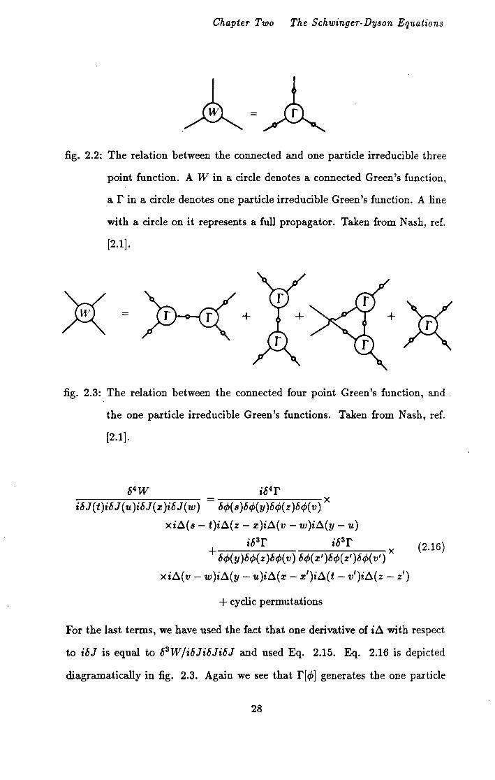
fig. 2.2: The relation between the connected and one particle irreducible three
point function. A W in a circle denotes a connected Green's function,
a r in a circle denotes one particle irreducible Green's function. A line
with a circle on it represents a full propagator. Taken from Nash, ref.
[2.1].
+
fig. 2.3: The relation between the connected four point Green's function, and .
the one particle irreducible Green's functions. Taken from Nash, ref.
[2.1].
64 W i64r i6J(t)i6J(u)i6J(z)i6J(w) = 6¢(s)6¢(y)6¢(z)6¢(v) x
xia(s- t)ia(z- z)ia(v- w)ia(y- u)
i63r i63r + 6¢(y)6¢(z)6¢(v) 6¢(z')6¢(z')6¢(v') x
(2.16)
xia(v- w)ia(y- u)ia(z- x')ia(t- v')ia(z- z')
+ cyclic permutations
For the last terms, we have used the fact that one derivative of ia with respect
to i6J is equal to 63W/i6Ji6Ji6J and used Eq. 2.15. Eq. 2.16 is depicted
diagramatically in fig. 2.3. Again we see that f[¢] generates the one particle
28

Chapter Two The Schwinger-Dyson Equations
irreducible Green's functions. Taking higher functional derivatives of Eq. 2.16
will reveal the same structure for the higher Green's functions, the general proof
going by induction.
We are now in a position to perform a perturbative expansion. First we
write
(2.17)
where S0 is the free action, and S1 contains any interaction terms. The free
action is quadratic in ¢,and we write it as
{2.18)
S 1 will in general be a polynomial in ¢ where we call each term a vertex.
For a vertex of order N, we can write its contribution to S1 as:
(2.19)
The perturbative series is generated by using the expansion
(2.20)
then any factors of ¢(z) which appear in Eq. 2.20 can be written as 6fi6J(z),
and taken outside the functional integral. Thus the perturbative solution for a
Green's function Gn(Zb···,zn) is
where Z0 [J] is the free field generating functional, Eq. 2.7. Here the functional
derivatives act on Z0 [ J] to bring down free field propagator factors. These are
29

Chapter Two The Schwinger-Dyson Equations
connected together by the vertices, such as that in Eq. 2.19. The lowest non-
trivial contribution to the Green's function GN(x 1 ,···,xN) for this vertex is
therefore seen to be:
For a connected Green's function, the free field propagators must connect
one x-variable to one y-variable in Eq. 2.22. This can be done in N! dif-
ferent ways, so we can simply read off the Feynman rule for this vertex as
i J ( n ~= 1 d4 y k) s N ( YI ' ••• ' y N). In momentum space, we simply take the Fourier
transform. For example, in >,.¢4 theory we have:
S1 = - >,.1 J d4 x¢4 (x)
4.
= - ; J ( fJ dz•) 6(x, - x, )6(x1 - x3 )6(x1 - z4 )if>(x, )if>(z,)if>(xa)if>(z4 )
(2.23)
From this we can read off the Feynman rule in momentum space to be -iA, as
usual.
Having set up the machinery, we are now in a position to derive our
equations, which relate the various Green's functions of the theory.
2.2 The Schwinger-Dyson Equations for Scalar Field Theory
The Schwinger-Dyson equations are derived from Z[J] by using the fact
that the functional integral of a derivative vanishes:
(2.24)
which gives us the functional equation
30

Chapter Two The Schwinger-Dyson Equations
j[D4JJ(6!~) + J(z)) exp (is+ i j d!y¢J(y)J(y)) = 0 (2.25)
Note the similarity of Eq. 2.25 to the classical equations of motion in the
presence of a source term:
6S 6¢J(z) + J(z) = 0 (2.26)
In this sense Eq. 2.25, and the equations we shall derive from it can be seen
. as the equations of motion of a quantum field theory. H we use the symbol
< H(z) > to denote the path integral of H(z) weighted by the exponential of
iS+ i J d"y¢(y)J(y), all divided by Z[O], then Eq. 2.25 can be written
6S hSo 6S1 < 6¢(z) > +J(z) = < 6¢J(z) > + < 6¢J(z) > +J(z) = 0 (2.27)
Let us find the contribution to this equation of our vertex of Eq. 2.19.
We have from Eq. 2.27:
(2.28)
where once again we have replaced ¢(Yi) by 6/ihJ(yi), and a repeated space
time index is to be integrated over. Taking the derivative with respect to the
classical field ¢(z2 ), Eq. 2.9, and using its definitions we obtain:
31

Chapter Two The Schwinger-Dyson Equations
where we have used the functional chain rule for differentiation in the second
term. Recognising -iS2 (x 17 x 2 ) as the inverse free propagator, and settin.g the
source term J equal to zero gives us the equation:
(i~(xl- x2))-1
= (i~o(xl- x2))-1
- (N ~ l)!iSN(xl,Yh" · · ,YN-l)Gn(Yl, · · · ,yN)(i~(YN- x2))-1
(2.30)
We can represent this equation diagramatically by noting that it states
that the full inverse propagator is equal to the free inverse propagator minus a
term which contracts the lowest order vertex iSN, with the full N-point Green's
function with the propagator on one external leg removed. For >.4>4 theory, we
use the form of the vertex in Eq. 2.23. Using the relations between the full
and connected Green's functions, Eq. 2.6, and then using the relations between
the connected and the one particle irreducible Green's functions, Eqs. 2.15 and
2.16., we obtain the equation depicted diagrammatically in fig. 2.4.
= -·~ -----~ -I
fig. 2.4: The Schwinger-Dyson equation for the inverse propagator in >.4>4 theory.
Taken from Nash, ref. [2.1).
This is the Schwinger-Dyson equation for the full inverse propagator
in >.4>4 theory. It is an integral equation, which relates the full two and four
point functions of the theory. Higher equations are simply derived by taking
more functional derivatives of Eq. 2.29. The resulting equation for the four
point function in >.4>4 theory is depicted in fig. 2.5. Here we can see that, in
general, the equation for then-point function involves contributions from up to
the (n+2)-point function.
32

Chapter Two The Schwinger-Dyson Equations
X I~. I +- +-2! ]!
fig 2.5: The Schwinger-Dyson equation for the four point function in ),<P4 theory.
Taken from Nash, ref. [2.1].
The form of Eq. 2.30 arises naturally in perturbation theory. Consider
a lowest order correction :E(p) which contributes to the self energy of the propa
gator in momentum space. Then the full perturbation series for the propagator
will contain the terms:
i.6.(p) = i.6.o(p) + i.6.o(p):E(p)i.6.o(p) + i.6.o(p):E(p)i.6.o(p):E(p)i.6.o(p) + · · ·
=i.6.o(p)(1 + i.6.o(p):E(p) + (i.6. 0(p):E(p))2 + ...
i.6.o (p) 1- i.6.o(p):E(p)
(2.31)
simply inverting this expression gives:
( i.6.(p)) - 1 - ( i.6.o(P)) - 1
- :E(p) (2.32)
which is identical in structure to Eq. 2.30.
2.3 Fermions and Path Integrals
A slightly different procedure is needed to deal with fermions, requiring
us to perform the functional integral over anticommuting, or Grassmann fields,
see ref. [2.1] for more details. In general though, for each fermion we introduce
two fields t/;, .,P and two anticommuting sources Tj, 1J· The fermionic part of the
path integral is then:
33

Chapter Two The Schwinger-Dyson Equations
The general n-point Green's functions are defined by:
(2.34)
In a similar way to before, we define W[f7, 17] and r['¢, '¢]. This time because of
the anticommuting nature of the fields we have as the parallel of Eq. 2.9:
6W .,P(x) = "6 ( )
l 1] X
- 6W .,P(x) = ·c ( )
-to1] X
6r fl(X) =- 6'¢(x)
6r ry(x) =~
'¢(x)
Thus the fermion propagator is defined as:
(2.35)
(2.36)
where a and /3 are spinor inclices, which we shall in general suppress. It can easily
be verified that i62 rj6'¢(x)6'¢(y) is the inverse fermion propagator. Similar
relations hold between the connected and the one-particle irreducible Green's
functions as for the scalar case.
2.4 The Schwinger-Dyson Equations for QCD
The path integral formulation of non-Abelian gauge theories has proved
to be the most intuitive way of formulating the full quantum field theory[2.3].
It is an elegant way of imposing the constraints of quantising a massless spin-1
34

Chapter Two The Schwinger-Dyson Equations
field, which has only the two transverse degrees of freedom as dynamical fields.
Because the path integration should really be over only gauge inequivalent fields,
we need to introduce a 'gauge fixing term'. This procedure also involves the
introduction of the so-called 'ghost' fields, which are anti-commuting. In an
Abelian theory, or in axial gauges for a non-abelian theory, these ghost fields
decouple. In covariant gauges however, they are an essential feature, preserving
the unitarity of scattering amplitudes, and the transversality of the gauge field.
This path integral formulation of a gauge theory is a well understood procedure,
and here we will merely write down the full QCD Lagrangian:
C = Cgauge + Cgauge-fix + C~host + Cquark (2.37)
where
C - - !pp.va F gauge -4
p.va
Cgauge-fix
(2.38)
Cquark = tPi(iDfjlp.- m)t/Jj
= tPi(ifJ- m)t/J + gTtjA11atPi/p.tPj
where Tri = >.fi /2 and ca, Ca are the ghost and anti-ghost fields respectively.
{is a parameter which fixes the gauge, where for example { = 0 is the Landau
gauge and { = 1 is the Feynman gauge. All the other quantities are defined in
section 1.3. The action is defined as:
35

Chapter Two The Schwinger-Dyson Equations
S = J cf'x.C(x) (2.39)
We can therefore write the pure gauge part of the action as:
where:
rabcd 0 p.vcrr
2
+ ~! rg~c:crr(xi' X2, xa, x4)A:(xi )At(x2)A~(xa)A~(x4)
- (r•· r•· [ 6,.6 .. - 6 •• 6,,] +/bee /dae [ h,.,.crhvr - hcrrhp.v]
(2.40)
+ , ... !'"' [ 6 •• 6,, - 6,.6 .. ]) 6( z, - z, )6( %3 - z. )6( z, - %3)
(2.41)
Once again it is implicit that repeated space-time variables are to be integrated
over. Here we recognise igf0~11 cr, ig2 f0~!crr as the bare triple and quartic gluon
couplings respectively[2.1]. Next we have:
36

Chapter Two The Schwinger-Dyson Equations
Sghost = J d4 x1Ca(xt)OCa (2.42)
+grg~c(x 1 , x2, X3 )A~c(x 1 )C\x2 )C6(x3)
where
(2.43)
is the bare ghost-gluon coupling. Finally we have:
(2.44) ~a a -+gA0 Ot/3 ij(xll x2, x3)A~(xi)'!f0ti(x2)tPf3j(x3)
where o and {3 are spinor indices, and
(2.45)
Following the form of Eq. 2.26, the Schwinger-Dyson equation for the
gluon field reads
fJS < -Ja fJA~(x) > = -~ (2.46)
Thus we obtain:
+g/2lrg~d17r(x,xbx2) < A 17c(.x1 )Ard(x2) >
+g2 /3!rg~d:rp(x,xbx2,x3) < A17c(x1)Ard(x2)Ape(x3) > (2.47)
-grg~d(x, xb x2) < Cd(x2)Cc(xt) >
-gA~:/3 ij(x, X}, X2) < tP{3j(X2)tPOti(xi) >
where the minus signs in the last two terms come from interchanging the order
of anti commuting fields. In terms of the classical field A~, and the connected
Green's functions we have:
3i

Chapter Two The Schwinger-Dyson Equations
(2.48)
where w,w are the sources for the ghost fields. Taking a further derivative with
respect to Ab (y) and setting J = A = 0 we obtain:
On multiplying by -i, and using Eqs. 2.13-2.16 which hold in identical form for
the gluon field, we obtain the Schwinger-Dyson equation {or the inverse gluon
propagator, first derived in ref. [2.4], and depicted diagramatically in fig. 2.6.
The relative minus sign of the last two terms in Eq. 3.49 can be ascribed to
38

Chapter Two The Schwinger-Dyson Equations
closed loops of anti-commuting fields.
Equations can similarly be derived for the ghost and quark propagators.
The equation for the quark propagator will be derived in chapter five. Until then
we consider a pure gauge theory, in which quark fields are absent.
Equations for the higher point Green's functions can also be derived, by
taking more functional derivatives of Eq. 2.48. It is easy to see from this that
the equation for the n-point gluon Green's function will involve contributions
from the 2, 3 · · · , n, n + 1, n + 2 point functions. Our equation for the propagator,
or two point function, is the first example of this, involving contributions from
the full 2, 3 and 4-point functions.
Since the Schwinger-Dyson equations are exactly satisfied by the full
Green's functions of the theory, by solving them we would hope to obtain infor
mation on the non-perturbative features of QCD, particularly that of confine
ment. Because there are infinitely many of these equations, one for each Green's
function, and all of them coupled, it is obviously an impossible task to solve them
exactly. Nevertheless we might hope to solve some truncated version of them.
This is in fact nothing more than we having been doing all along in perturbation
theory. The simplest truncation possible of the Schwinger-Dyson equations is
to ignore all terms involving loops. We are left with equations which state that
the 2,3 and 4-point functions are equal to the corresponding bare ones appear
ing in the classical Lagrangian, with the higher Green's functions all vanishing.
We can then take these solutions and substitute them in the right hand side
of the Schwinger-Dyson equations. Thus Eq. 2.49, for example, will generate
the :first few terms of the perturbative expansion of the inverse gluon propa
gatpr. More exactly, perturbation theory is nothing else than the solution to
the Schwinger-Dyson equations based on a truncation in succesive powers of the
coupling constant. Of course, perturbation theory is a very special truncation,
in that it satisfies the requirements of renormalisability and unitarity, i.e. it
39

Chapter Two The Schwinger-Dyson Equations
- / 1 ' I
I \
~ ' ' /
' /
I II
-I
fig 2.6: The Schwinger-Dyson equation for the gluon propagator in QCD. The
curly lines represent gluons, the dotted lines ghosts. A dark circle on a
line represents a full propagator, a dark circle on a vertex represents a
full one particle irreducible vertex. We have not included the fermion
contribution, for this see chapter six.
40
Chapter Two The Schwinger-Dyson Equations
allows a systematic removal of the ultraviolet infinities, to give answers in which
quantum mechanical probabilities are conserved. These are essential features in
the calculation of physical quantities.
This thesis details an entirely different truncation of the Schwinger
Dyson equations, in which quantities are not truncated at some particular order
in the coupling constant, and so contain some information to all orders in g. In
this way we might hope to attack the non-perturbative region of QCD. That
'this truncation has yet to be made entirely consistent in the way perturbation
theory is, should not deter us. At the best, we may eventually discover a fully
consistent non-perturbative treatment of QCD. At the worst, we might still
expect to divine some of the salient features of the theory.
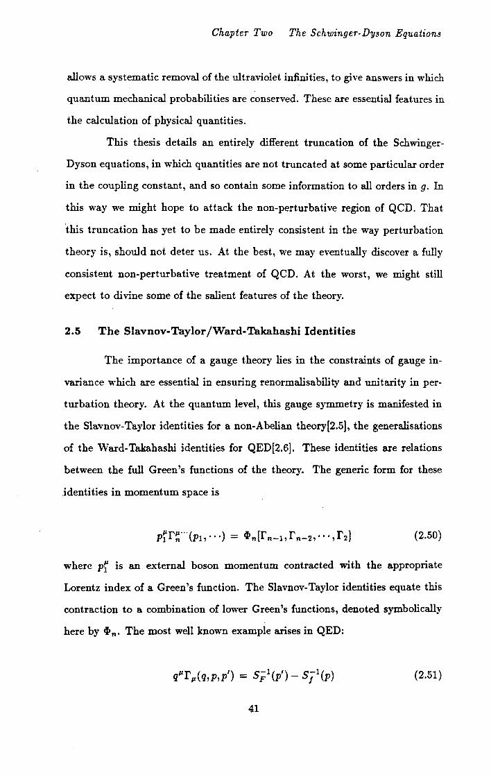
2.5 The Slavnov-Taylor /Ward-Takahashi Identities
The importance of a gauge theory lies in the constraints of gauge in
variance which are essential in ensuring renormalisability and unitarity in per
turbation theory. At the quantum level, this gauge symmetry is manifested in
the Slavnov-Taylor identities for a non-Abelian theory[2.5], the generalisations
of the Ward-Takahashi identities for QED[2.6]. These identities are relations
between the full Green's functions of the theory. The generic form for these
.identities in momentum space is
(2.50)
where Pi is an external boson momentum contracted with the appropriate
Lorentz index of a Green's function. The Slavnov-Taylor identities equate this
contraction to a combination of lower Green's functions, denoted symbolically
here by ~n· The most well known example arises in QED:
q~'r p(q,p,p') = Sil(p')- Sjl(p)
41
(2.51)

Chapter Two The Schwinger-Dyson Equations
where fll(q,p,p') is the full electron-photon three point irreducible Green's func
tion, q is the incoming photon momentum, equal top' - p, and SF is the full
electron propagator. This identity holds for the full Green's functions, but also
holds order by order in perturbation theory. Thus to lowest order r ll = -i-yll,
SF= i/p, and Eq. 2.51 holds trivially.
In general we can divide such a vertex into a longitudinal and a trans
verse piece[2.7], where the transverse piece is defined by the property that it
vanishes when contracted with any external boson momenta. i.e.
(2.52)
where we have
'Vi (2.53)
The transverse part is obviously unconstrained by the Ward identities.
Moreover, this split is not unique because we can always add an arbitrary amount
of the transverse part to the longitudinal part. We can ensure uniqueness,
however, by demanding that fL be free of kinematic singularities. Since the
complete vertex must also be free of kinematic singularities, then the transverse
part must be as well. The important point about this condition, is that in general
it allows us to 'solve' the Ward identity for the longitudinal vertex in terms of
the lower Green's functions in a unique way. The best way of demonstrating
this is to give an example.
In scalar electrodynamics, we have a three-point vertex describing the
interaction of the photon with a charged scalar particle. The Ward identity for
this vertex reads[2. 7]:
(2.54)
42
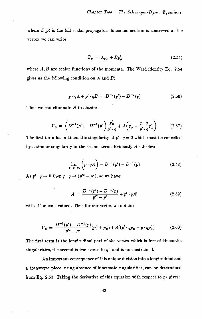
Chapter Two The Schwinger-Dyson Equations
where D(p) is the full scalar propagator. Since momentum is conserved at the
vertex we can write
(2.55)
where A, B are scalar functions of the momenta. The Ward identity Eq. 2.54
gives us the following condition on A and B:
(2.56)
Thus we can eliminate B to obtain:
r = (n-1(p')- n-1(p)) P~ + A(p - P · q p') ll p'·q ll p'·q ll
(2.57)
The first term has a kinematic singularity at p' · q = 0 which must be cancelled
by a similar singularity in the second term. Evidently A satisfies:
lim (P · qA) = n-1(p')- n-1(p) p'·q-o
Asp'· q-+ 0 then p · q-+ (p'2 - p2 ), so we have:
A = n-l(p')- n-l(p) + p'. qA' p'2- p2
with A' unconstrained. Thus for our vertex we obtain:
(2.58)
(2.59)
(2.60)
The first term is the longitudinal part of the vertex which is free of kinematic
singularities, the second is transverse to q~'- and is unconstrained.
An important consequence of this unique division into a longitudinal and
a transverse piece, using absence of kinematic singularities, can be determined
from Eq. 2.53. Taking the derivative of this equation with respect to Pi gives:
43

Chapter Two The Schwinger-Dyson Equations
r"'l ···11···1-'n + p'!"i _!!__ rl-'1"""1-'i ···1-'n = 0 (2.61) T I 8p'[ T .
From our previous discussion we have obtained a rT which is itself free from
kinematic singularities. Thus as Pi - 0 the second term must vanish. From Eq.
2.61 we therefore deduce that rT itself vanishes in this limit that the external
momenta go to zero. In other words by splitting the vertex as we have done, the
low momentum behaviour is given entirely by the longitudinal part, precisely
the piece we can determine from the Ward identity. This result is of much
importance in a non-Abelian theory, in which it is the low momentum behaviour
of Green's functions which cannot be determined in perturbation theory, and
which we wish to investigate.
We are now in a position to outline the approach we will take to solve
the Schwinger-Dyson equations[2.8]. We can write the full hierarchy of equations
symbolically as follows:
r2 =n2[r2,r3,r4]
r3 =na[r2,r3,r4,rs]
(2.62)
Here r n represents the n-point gluon Green's function, and nn the relevant
combination of Green's functions. The first thing we do is to truncate the
equations at, say, the equation for r n• If we first set r n+2 = o, and then set
r n+l equal to its longitudinal part in the expression for nn, then we will have a
closed set of equations which we can think about solving. Since the longitudinal
part of r n+I gives the exact behaviour in the zero momentum limit, we should
expect this to be a valid ·approximation in which to study the low momentum
44

Chapter Two The Schwinger-Dyson Equations
behaviour of Green's functions. The neglecting of the terms involving r n+2 can
also be justified (see section 3.1 ). The procedure is to solve this truncated version
of the equations for n = 2. We would then repeat the procedure for n = 3 and
higher until the solutions for the lower Green's functions remain stable as we
increase n.
The first step then, is to consider the equation for the gluon propagator,
Eq. 2.49. In practice it will probably not be possible to go beyond this first
equation, because of the increasing complexity of the problem, which in general,
requires numerical techniques to find a solution. Moreover, the Schwinger-Dyson
equation for then-point function is in general a multitude of tensor equations.
The equation for three point triple gluon vertex for example, can be divided into
14 coupled equations[2.7], and so attempting to treat this equation will need an
extraordinary amount of computing power. Nevertheless, by considering this
first equation, we might hope to extract some indication as to the low momentum
behaviour of the gluon propagator. This in turn may help us understand the
non-perturbative aspects of gluons.
Before we do this, however, we must consider the Slavnov-Taylor iden
tities for QCD. These have the same general features as in Eq 2.50, although
the situation is complicated by ghost terms. Also, from now on we work in
Euclidean space. This is partly because quantum field theories are really only
defined in Euclidean space[2.1], with a Wick rotation to Minkowski space to
be performed at the end of a calculation. Moreover, in perturbation theory,
in order to perform the integrals that arise in higher order corrections, and to
isolate their divergent parts, we usually use the technique of 'dimensional reg
ularisation', which again, is really only defined in Euclidean space. The use of
Euclidean space also eases the numerical integrations we shall perform in later
chapters.
First of all we introduce the full gluon propagator in a covariant gauge:
45

Chapter Two The Schwinger-Dyson Equations
tl. /lll ab (
Q(p) (6''v- pllpV) + {piLpV) Dab p2 p4 (2.63)
where {is our gauge parameter. Here we are working in momentum space. The
tensor structure of Eq. 2.63 is determined by the Slavnov-Taylor identity for
the gluon propagator which ignoring colour indices reads:
(2.64)
where flllv is the inverse gluon propagator. This means that the longitudinal part
of the full gluon propagator is equal to that of the free propagator, so that the
full propagator is an undetermined transverse piece plus the free longitudinal
part, as in Eq. 2.63. The full non-perturbative content of the propagator is
contained in the gluon renormalisation function 9(p).
The full ghost propagator is simply a scalar function of p2 :
H(p) tl.ab(P) = Dab_2_
p
Finally we decompose the ghost gluon vertex as:
(2.65)
(2.66)
where r 11 is the anti-ghost incoming momentum, and p is the incoming gluon
momentum.
We write the full triple gluon vertex as r:~: (p, q, r) = /abcrpvt7 (p, q, r)
In terms of these quantities the Slavnov-Taylor identity for the full triple gluon
vertex reads:
q•r , •• (p, q, r) = H(q) { - Q;r) (h .. r 2 - r' r"}r ,,(p, q, r)
+ 9;p) W' P'- p'p')r .. (r,q,p)}
46
(2.67)

Chapter Two The Schwinger-Dyson Equations
This can be solved[2. 7] to determine the longitudinal part ~f r p.vcr(P, q, r) which
is free of kinematic singularities, in terms of the ghost-gluon vertex, and the
ghost and gluon propagators. From Eq. 2.67 we see that:
(2.68)
and this, with its cyclic permutations, provides further constraints on the vertex.
Further simplifying approximations can be used if we work in the Lan-
dau gauge (e = 0)[2.9,1.6]. We can write the full ghost-gluon vertex diagram-
matically as in fig. 2.7. This is essentially the Schwinger-Dyson equation for
this vertex. It says the full ghost-gluon vertex is equal to the bare one, plus a
ghost-gluon scattering kernel. This kernel is proportional to rP. from the external
anti-ghost line, and .contains a term 1P,6."P(q -1) = qP,6."P(q -1), by using the
fact that the gluon propagator is transverse in this gauge. Thus this kernel is
proportional to rP.q" and so vanishes when one of these external momenta goes
to zero. In this limit the full ghost-gluon vertex is equal to the bare one, and
we haver P." = 6,. 11 • This considerably simplifies the Slavnov-Taylor identity Eq.
2.67. Again since it is the low momentum behaviour of the theory we wish to
determine, we can use this simplification.
A +
Q
fig. 2. 7: Equation for the full ghost-gluon vertex. A wavy line denotes a gluon,
a curly line denotes a ghost. The black dots denote an anti-ghost line.
The momenta are labelled. Taken from Marciano and Pagels, ref. [1.6].
If we now consider:
47

Chapter Two The Schwinger-Dyson Equations
p" q11 r 1'110' (p, q' r) (2.69)
-we can perform the two contractions in either order. Performing the q11 contrac-
tion first and t].sing the simplified Slavnov-Taylor identity of Eq. 2.67 we obtain
the expression:
(2.70)
On the other hand, if we perform them the other way round we obtain the
expressiOn:
(2.il)
and these two expressions must be equal. Since p+q+r = 0, we have p = -q-r.
The tensors in Eqs. 2. 70 and 2. 71 are transverse, and vanish when contracted
with r. Thus the tensor parts are equal, and hence we deduce that H(p) = H(q).
Thus the ghost propagator function His a constant which we set equal to one, its
bare value. We therefore obtain the final version of the Slavnov-Taylor identity
for the triple gluon vertex:
q~'f pvu(p, q, r) (2.72)
This can be 'solved' for the longitudinal part of the triple gluon vertex[2.7) to
g~ve:
48

Chapter Two The Schwinger-Dyson Equations
(2.73)
We shall use this form of the triple gluon vertex in the next chapter.
For completeness we give the Slavnov-Taylor identity for the quark
gluon vertex rrja(q,p,p')[2.7]:
(2.74)
where Aij( q,p,p') is a ghost-quark scattering kernel, similar in form to the ghost
gluon scattering kernel in fig. 2.7. As before, it can be shown that as the external
momenta go to zero, that Aij(q,p,p') behaves like Tlj,. the bare kernel[2.9]. This
is simply the colour matrix of rr;a = Tljf~-', and so using this low momentum
approximation the Slavnov-Taylor identity of Eq. 2. 74 reduces to an Abelian-like
Ward identity to give:
(2.75)
For massless quarks we have Sp(p) = :F(p)jp, and the identity of Eq. 2.75 can
be solved for the longitudinal part of the vertex[2.7], to give:
49
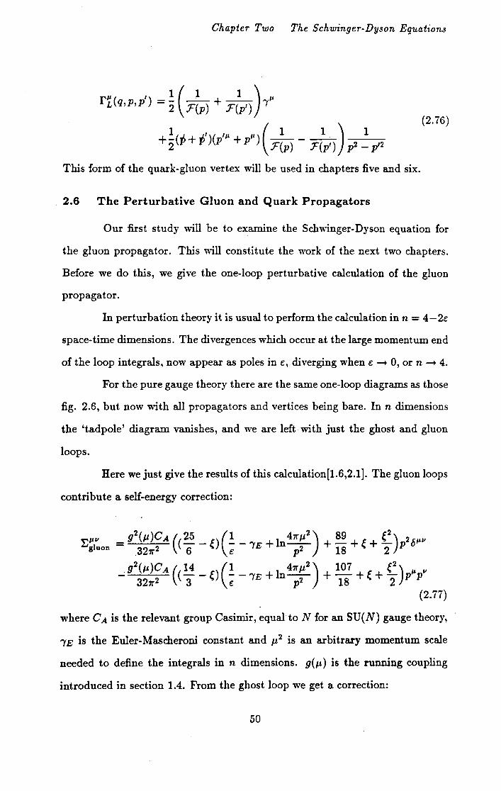
Chapter Two The Schwinger-Dyson Equations
(2.76)
This form of the quark-gluon vertex will be used in chapters five and six.
2.6 The Perturbative Gluon and Quark Propagators
Our first study will be to examine the Sch·winger-Dyson equation for
the gluon propagator. This will constitute the work of the next two chapters.
Before we do this, we give the one-loop perturbative calculation of the gluon
propagator.
In perturbation theory it is usual to perform the calculation inn= 4-2e
space-time dimensions. The divergences which occur at the large momentum end
of the loop integrals, now appear as poles in e, diverging when e-+ 0, or n-+ 4.
For the pure gauge theory there are the same one-loop diagrams as those
fig. 2.6, but now with all propagators and vertices being bare. Inn dimensions
the 'tadpole' diagram vanishes, and we are left with just the ghost and gluon
loops.
Here we just give the results of this calculation[1.6,2.1]. The gluon loops
contribute a self-energy correction:
where C A is the relevant group Casimir, equal toN for an SU(N) gauge theory,
"YE is the Euler-Mascheroni constant and p,2 is an arbitrary momentum scale
needed to define the integrals in n dimensions. g(p,) is the running coupling
introduced in section 1.4. From the ghost loop we get a correction:
50

Chapter Two The Schwinger-Dyson Equations
(2.i8)
Adding these together gives
Note that this correction is transverse, and so the Slavnov-Taylor identity for
the gluon propagator Eq. 2.64 holds. Essentially this identity states that the
longitudinal part will not get renormalised by higher order corrections, and we
see that this is indeed the case.
Although the ghost corrections are essential in preserving the transver
sality of the higher order corrections to the propagator, we see that for 'sensible'
gauges, such as e = o, they make a numerically small contribution of less than
10%. This provides further support for our neglect of the ghost terms in section
2.5.
Renormalisation consists of subtracting the poles in e. We use the MS
scheme which also subtracts the "'E and ln411" factors, to give the renormalised
self-energy
{2.80)
Since we have:
(2.81)
we can invert this to extract:
51
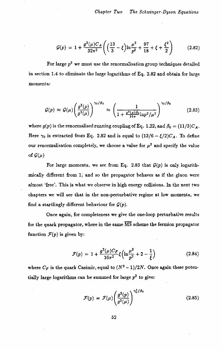
Chapter Two The Schwinger-Dyson Equations
(2.82)
For large p2 we must use the renormalisation group techniques detailed
in section 1.4 to eliminate the large logarithms of Eq. 2.82 and obtain for large
momenta:
(2.83)
where g(p) is the renormalised running cou piing of Eq. 1.22, and /30 = ( 11/3) CA.
Here "'Yo is extracted from Eq. 2.82 and is equal to (13/6- {/2)CA. To define
our renormalisation completely, we choose a value for p,2 and specify the value
of Q(p,)
For large momenta, we see from Eq. 2.83 that Q(p) is only logarith
mically different from 1 ,' and so the propagator behaves as if the gluon were
almost 'free'. This is what we observe in high energy collisions. In the next two
chapters we will see that in the non-perturbative regime at low momenta, we
find a startlingly different behaviour for Q(p).
Once again, for completeness we give the one-loop perturbative results
for the quark propagator, where in the same MS scheme the fermion propagator
function :F(p) is given by:
:F(p) = 1+g2(p,)CFe(InJl2 +2-!) 1611'2 . p2 e (2.84)
where CF is the quark Casimir, equal to (N2 -1)/2N. Once again these poten-
tially large logarithms can be summed for large p2 to give:
(g2(p)) "Y~//3o
:F(p) = :F(p,) g2 (p,)
52
(2.85)

Chapter Two The Schwinger-Dyson Equations
where ici = f.CF.
The introduction of quarks introduces a closed fermion loop in the
calculation for the gluon propagator. This merely changes the form of 'Yo to
(13/6- {/2)CA- (4/3)ntTF, and changes f3o to (11/3)CA- (4/3)ntTF in Eq.
2.83. Here TF is a colour trace, with TF = 1/2 for QCD.
We now return to a world without quarks, and attempt to solve the
truncated Schwinger-Dyson equation for the gluon propagator, using the ap
proximations outlined in section 2.5.
53

Chapter Three The Gluon Equation
CHAPTER THREE
THE GLUON EQUATION
3.1 Derivation of the Equation for 9(p)
We now proceed to derive a closed equation for the gluon renormali
sation function Q(p), following the procedure outlined in section 2.5[3.1]. The
complete Schwinger-Dyson equation for the inverse gluon propagator, depicted
in fig. 2.6 involves the unknown triple and quartic gluon vertices, as well as the
ghost contributions. In order to derive a closed equation for the gluon renor
malisation function we must make some approximations.
The first step is to ignore those diagrams which involve quartic gluon
couplings, (see section 2.5). This can be seen as a first step in an iterative
procedure to solve the entire heirarchy of the Schwinger-Dyson equations. Per
haps more realistically, we note that these diagrams contain an explicit factor
of a5, where ao = g5/4rr is the bare coupling. When we come to renormalise
our equation (see section 3.3), we will do this at some scale tt2 , which we will
choose to be in the perturbative regime. The bare couplings which appear in
the unrenormalised equation will be replaced by the renormalised running cou
pling a(J.L ), which, since J.L2 is in the perturbative region, will be a small number.
Hence these diagrams involving the quartic couplings will be suppressed by a
factor a(tt) relative to the remaining terms. Of course, the value of the loop
integral could swamp this suppression, but it seems natural to believe that the
triple gluon vertex already contains the seeds, if not all the details, of a confining
mechanism.
Next we consider the ghost diagram. Since we choose to work in the
Landau gauge, then as was seen in section 2.5, it is believed that the ghost
kernels which appear in the Slavnov-Taylor identites for both the triple gluon
vertex, and the quark-gluon vertex, will vanish as one of the external momenta
54

Chapter Three The Gluon Equation
goes to zero. Although the ghost contributions are essential in preserving the
transversality of the inverse gluon propagator, it is to be hoped that they will
not play a significant role in the analytic behaviour of 9(p ). This is supported by
the fact that in a one-loop perturbative calculation, the ghost loop (see section
2.6) makes a numerically small contribution to 9(p), at least for the Landau,
and other 'sensible' gauges.
Our equation still involves the full triple gluon vertex. In the light of the
above comments on the infra-red vanishing of the ghost kernels, by setting them
identically to zero, we can 'solve' the Slavnov-Taylor identity for this vertex
entirely in terms of 9(p). This was done in section 2.5. This allows us to
completely determine the longitudinal part of the vertex; the Slavnov-Taylor
identity does not constrain any transverse part. Fortunately it can be shown,
Eq. 2.61, that as one of the external momenta ofthe vertex goes to zero, then the
transverse part vanishes. In QCD it is precisely the low momentum behaviour
which cannot be determined by perturbation theory, and it is in this region that
our various approximations made are likely to be valid. Thus we set the full
triple gluon vertex equal to its longitudinal part, determined in terms of g from
the Slavnov-Taylor identity in the absence of ghosts.
At this stage we do not include the contributions of quarks, which would
contribute a quark loop diagram to our equation. If this were included, we would
have to consider the Schwinger-Dyson equation for the fermions as well. This
problem is addressed in chapters five and six. For the moment we consider only
the pure gauge theory, as we expect that it is the non-Abelian nature of the
gauge part of the theory which is responsible for confinement.
After all these approximations, we have managed to derive a closed
equation for the gluon function 9(p):
II"'" II"'" "C"'Il" ab = Oab - ~ab
55
(3.1)

Chapter Three The Gluon Equation
Here IT represents the full inverse gluon propagator, ll0 the bare one, and ~ is the
contribution to the gluon self-energy from the equation depicted diagramatically
in fig. 2.6, neglecting the ghost and two-loop terms. The colour indices of Eq.
3.1 are given on both sides by hab, and we factor this out. We project with the
tensor
{3.2)
to give a scalar equation. This tensor gives zero when contracted with hllv, and
gives 1 when contracted with pllpv. The contribution of the tadpole diagram
in fig. 2.6 is as usual proportional to hllv and so this contribution vanishes.
Thus the only diagram contributing to the self-energy is the gluon loop diagram
shown in fig. 3.1 which we now calculate.
k
p-k
fig. 3.1: The gluon loop contributing to the truncated Schwinger-Dyson equation
for the inverse gluon propagator.
56

Chapter Three The Gluon Equation
3.2 The Gluon Loop
We can write out our eguation as:
Q~p) = 1 + ~57r~;2 P11 v j d4kr~06 ( -p, k, q)iln,B(k )il..,6(q)r~"..,( -k,p, -q)
(3.3)
where r~06 (-p,k,q) is the bare triple gluon vertex, and r~""Y(-k,p,-q) is the
longitudinal part of the full triple gluon vertex, which we take to be given by
Eq. 2.73. The momenta are as labelled in fig. 3.1. Working in the Landau
gauge, the full gluon propagator is given by:
where:
We write the integrand in Eq. 3.3 as Q(k)Q(q)IIl" fk 2q2 , with:
If" = r~n6 ( -p, k, q)6n,86..,6r~"..,( -k,p, -q)
I:" = r~n6 ( -p, k, q)kok,86..,6r~"..,( -k,p, -q)
I:" = r~n6 ( -p, k, q)6nflq..,q6r~".., ( -k,p, -q)
I:" :.... r~06 ( -p, k, q)kokflq..,q6r~"..,( -k,p, -q)
(3.4)
(3.5) .
(3.6)
We can now use the Slavnov-Taylor identites in the absence of ghost
contributions:
(3.7)
57

Chapter Three The Gluon Equation
which are satisfied by the vertices in Eq. 3.3 (see Eq. 2.72), to simplify some of
the expressions in Eq. 3.6. Some easy tensor algebra gives:
If" is identical to I:", but with k and q interchanged. We also have:
If" is more complicated. After performing the Lorentz contractions in Eq. 3.6
it is equal to r~rh(-p,k,q)r~"-r(-k,p,-q), which from Eqs. 2.73 and 2.41 we
write as:
(3.10)
After performing the Lorentz contractions we obtain:
58

Chapter Three The Gluon Equation
Note that the integrand is symmetric between k and q, as it should be. Using
this symmtry, we can replace I:'' I q2 with I:" I k2 , and we can also simplify If",
writing it as:
Projecting with the tensor P~", Eq. 3.2, we obtain:
1 I~" p = --(p2(p. k)2- k2p4)
4 "" 3Q(p) (3.13)
59

Chapter Three The Gluon Equation
Next we have:
Finally we split lf 11 into four terms:
p 2 ( 1 1 ) (6/JII )2 2 iJ II iJII p2 - q2 Q(p) - Q(q) (p + q p' q + 4p q q
-p. qp/Jpll- (q2 + 2p. q)piJqll- 4p. qq/Jpll)
2 ( 1 1 ) 1 ( )2 2 2 2 2) = - - - - - 2(p. q - 3q p. q - 3p p. q- 4p q p2 - q2 Q(p) Q(q) 3
=- - - - - 12p + 24p p. k + 3k p. k 2 1 ( 1 1 )( 4 2 2 3 p2- q2 Q(p) Q(q)
- 7k2p
2- B(p • k)2
)
60
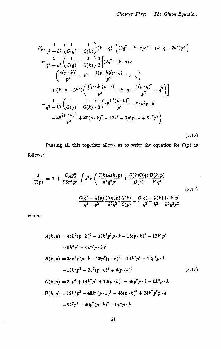
follows:
where
Chapter Three The Gluon Equation
(3.15)
Putting all this together allows us to write the equation for Q(p) as
Q(q)- Q(p) C(k,p) Q(k) + Q(q)- Q(k) D(k,p) q2- p2 k2q2 Q(p) q2 - k2 k2q2p2
A(k,p) =48k2(p · k)2 - 32k2p2p · k -16(p. k)8 -12k4p2
+6k2p4 + 6p2(p. k)2
B(k,p) =38k2p2p · k- 25p2(p. k)2 -14k2p4 + 12p4p. k
-13k4p2 - 2k2(p. k)2 + 4(p. k) 3
C(k,p) = 24p4 + 14k2p2 + 16(p · k)2 - 48p2p · k- 6k2p. k
D(k,p) = 12k4l- 48k2(p · k)2 + 48(p · k)3 + 24k2p2p · k
-5k2p4 - 40p2(p. k)2 + 9p4p. k
61
(3.16)
(3.17)

Chapter Three The Gluon Equation
This is the equation we have to solve. As it stands, however, the integrals have
ultraviolet logarithmic divergences, as well as potential infra-red divergences.
These must be dealt with to give us a finite renormalised equation.
3.3 Renormalisation
As we shall later argue, the only possible consistent behaviour for 9(p)
as p2 --+ 0 is 9 (p) "' 1/ p2• If 9 (p) is this singular, however, the integrals in
Eq. 3.16 are potentially infra-red divergent. In a related study in the axial
gauge[3.2], such divergences are avoided by assuming that: (i) the full axial
gauge propagator has the same tensor structure as the bare one, and (ii) that
the coefficient of such an infra-red enhanced term is independent of the choice of
axial gauge. It is possible that if we could solve the complete Schwinger-Dyson
equation with no approximations or truncations, then such a term would not
give rise to divergences. Nevertheless, as they do appear in our truncation, we
must deal with them. We choose to treat them by defining 9(p) by a 'plus'
prescription, which we define later in section 3.5. Of course, this prescription
is not determined by the theory, but put in 'by hand'. In chapter five, and
in other work[3.3], different treatments are used, but the justification here will
lie in the physically meaningful results we obtain. One of the long term goals
of any analysis based upon the Schwinger-Dyson equations will be to eliminate
these infra-red divergences in a self-consistent way, entirely within the context
of the theory. A fuller discussion of this and other infra-red problems appears
in chapter seven.
Even when we have dealt with these divergences, we still obtain contri
butions violating the masslessness of the gluon, a condition demanded by gauge
invariance. If 9(p) has such an infra-red singular term, on dimensional grounds
it must be AJ.t2 jp2 • Even after integration, the dimensionful quantity 112 must
be balanced, and the only quantity available is p2 • Thus we get contributions
62

Chapter Three The Gluon Equation
to the right hand side of Eq. 3.16 which behave like 1/p2 • The condition for
masslessness is:
(3.18)
where IT~'" is the full inverse gluon propagator. Since the bare inverse gluon
propagator obeys the condition Eq. 3.18, then all our integrals on the right
hand side of Eq. 3.16, ·must obey this as well. This is clearly not true of some
of the terms which arise from integration of the infra-red enhanced term. We
must perform a subtraction to remove these terms. Formally, we may imagine
some appropriate counter-terms in the bare Lagrangian to achieve this
The easiest way to preserve masslessness is to write Q(p) = AJ12 fp2 + 9 1 (p), where p2Q1 (p)--+ 0 as p2 --+ 0. The entire contribution to the mass term
comes from the enhanced term AJJ2 fp2• Thus if in the right hand side of Eq.
3.16 we set Q(p) = AJ12 fp2 and subtract this from Eq. 3.16, then no mass
term will arise. Note that if the mass term should be equal to zero, then the
term subtracted will vanish as well. This mass renormalisation, and the 'plus'
prescription treatment of the infra-red divergences do not prejudge that Q(p)
does possess such an infra-red enhanced term, as we allow the possibility that
the coefficient of this term can vanish. Finally, any terms on the right hand
side of Eq. 3.16 which are linear in Q will have the entire contribution of the
enhanced term subtracted by this mass renormalistaion. In these terms we can
effectively set Q = Q1 •
We still have the usual logarithmic ultraviolet divergences, which arise
from the momentum loop integral at large k2 • To handle these we cast Eq. 3.16
into the form:
1
Q(p)
63
(3.19)

Chapter Three The Gluon Equation
where:
(3.20)
C(k,p) = 9(q)B(k,p) + C(k,p) [9( ) - 9( ) (P2 + J.l2 )] 1 k4q4p2 q2- p2 q p q2 + J.l2 k2q2p2
Here JC(k,p) contains those terms which are linear in 9, whereas C(k,p)
contains those terms which are quadratic in 9 in the numerator, with an explicit
1/9 (p) in the denominator.
In splitting the integral into these two tem1s, there is a slight tech
nicality over the term proportional to C(k,p), which involves the factor
(9(k)/9(p))(9(q)- 9(p))/(q2 - p2). This term contains a part which belongs to
JC(k,p) and a part belonging to C(k,p). These will be renormalised differently,
and so we must be careful not to introduce any singularities from the q2 - p2
term in the denominator. This is done by writing:
(3.21)
Here we call the first term part of C(k,p) and the second term part of JC(k,p).
All we have done is to add and subtract at term which ensures both parts are
individually finite at p2 = q2 • This term is obviously arbitrary, but we have
chosen it so that it does not introduce any extra ultraviolet divergences, being
finite by power counting. The momentum p.2 in Eq. 3.21 is also arbitrary, but
for convenience we choose it equal to our renormalisation scale.
64
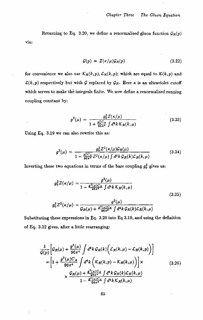
Chapter Three The Gluon Equation
Returning to Eq. 3.20, we define a renormalised gluon function 9R(P)
VIa:
(3.22)
for convenience we also use X:R(k,p), .CR(k,p); which are equal to X:(k,p) and
.C(k,p) respectively but with 9 replaced by 9R· Here K is an ultraviolet cutoff
which serves to make th~ integrals finite. We now define a renormalised running
coupling constant by:
D2(J-t) = g5Z(K/Jt)
1 + ~~~: j d4kX:R(k,p) (3.23)
Using Eq. 3.19 we can also rewrite this as:
(3.24)
Inverting these two equations in terms of the bare coupling 95 gives us:
2z("'/ ) - g2(J-t) Do J-t - 1 - a,<e>cA fd4k X: (k )
9611"4 R 'J-l
(3.25)
2 z2(~ef ) - g2(J-t) Do J-t - 9R(J-t) + 92Jg~~A J d4k9R(k).CR(k,p)
Substituting these expressions in Eq. 3.25 into Eq 3.19, and using the definition
of Eq. 3.22 gives, after a little rearranging:
Qtp) [QR(J-t) + ~:~: J tf4k QR(k) ( .CR(k, J-t)- .CR(k,p))]
= [ 1 + D2
~~~; A J trk ( X:R(k,p)- X:R(k,p)) l X (3.26)
QR(J-t) + 92J:~~A j d4k 9R(k)£R(k,p) X _...:..:_:._~~:::--=---___;___:_____;__..;_
1-92J:~?A J d4kX:R(k,p)
65

Chapter Three The Gluon Equation
The quotient in the third line of Eq. 3.26 is seen to be simply 1 I Z (,..I Jl) from
Eq. 3.25. This can be used to renormalise the factor of 1l9(p) on the left hand
·side of Eq. 3.26 to give us the renormalised equation in which all integrals will
be ultraviolet finite:
(3.2i)
In the next section, we will need a more explicit form for the running
coupling, in order to determine the behaviour of 9n(p) at large p2 • We first
invert Eq. 3.23 to give:
(3.28)
subtracting Eq. 3.28, from the same equation evaluated at p gives:
(3.29)
If we take the definition of Eq. 3.22, and instead renormalise at p2 we would
have:
9(p) = Z(Kip)9n,(P) (3.30)
where for clarity we have written the subscript Rp to denote. that p2 is our
renormalistaion scale. However we must have 9 n, (p) = 9 R,. (Jl), and we rewrite
Eq. 3.30 as:
(3.31)
Then the equality of Eqs. 3.22 and Eq. 3.31 allows us to write:
66

Chapter Three The Gluon Equation
9R(p) 9R(Jl)
(3.32)
where all quantities are renormalised at the scale 112 • This allows us to simply
rewrite Eq. 3.29 as:
(3.33)
as an equation for the renormalised running coupling constant. We have given
the deri-vation of Eq. 3.33 in some detail, as the same sort of arguments will be
used to define the other running couplings which will appear in our study.
3.4 Consistent Asymptotic Behaviour of 9R(P)
Because of the complicated structure of our equation for the gluon renor
malisation function 9R(p), Eq. 3.27, an analytic solution is not possible, and
we attempt a numerical study. Before we do this, we investigate the possible
asymptotic behaviour for both small and large p2 that we should build into our
numerical solution. In general we will take a trial input function 9in(p), and
substitute this into the right hand side of our equation, Eq. 3.27. After per
forming the integrals we obtain an output fu~ction 1/9out(p), to be compared
to the reciprocal of the input function. We allow our trial function to depend
on a number of parameters, and we vary these until we find good agreement
between input and output over a suitable range of p2 •
All of the integrals in Eq. 3.27 give rise to dimensionless quantities, and
all contain the factor 1/ k2 q2 in their denominator. This allows us to derive the
following general results
a) H 9in(P) _... constant, as p2 _... 0, then the output of the right hand side of
Eq. 3.27 is easily seen to give:
1 ~ = 1 + (constant)ln(p2 /112
) ~out
67

Chapter Three The Gluon Equation
b) If 9in (p) "' lnp2 as p2 -t 0, then the right hand side gives:
1 ;::;--- = 1 + constant In 2 (p2 j JL 2 ) ~out
c) These logarithms may sum to a power. If we let 9in(P) -t (p2 jp2 ) 0 as p2 -t 0
with a < 1, then all the integrals are infra-red finite, and we would obtain:
-- = 1 + constant JL 2
1 ( 2) 0
9out P
where this is purely on dimensional grounds, to balance the dimensionful quan
tity p 2 •
In all of these cases it is not possible to obtain agreement between input and
output. If, however, we consider the case 9in -t p 2 /p2 , and we use some regu-
larisation technique to deal with the infra-red divergences, then we would find
by the same dimensional arguments that
where Cis a constant. Unlike the terms in c) above, this will violate our mass
lessness condition, and so must be subtracted. Then if the higher order terms
in p2 of Q(p) generate a contribution to the right hand side of which cancels the
explicit factor of 1, then the right hand side of the equation would vanish as
p2 -t 0. This is exactly the behavior of the left hand side, and we have the pos
sibility of finding agreement. If the next order p2 corrections to 9in(P) behaved
like a constant, a logarithm, or a power as in c) above, but with 0 <a < 1, then
this would give rise to inconsistent behaviour, as the left hand side of Eq. 3.27,
i.e the reciprocal of the input function vanishes at small p2 • We therefore will
attempt to find solutions which behave like:
68
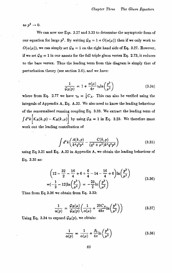
Chapter Three The Gluon Equation
as p2 -+ 0.
We can now use Eqs. 3.27 and 3.33 to determine the asymptotic form of
our equation for large p2• By writing 9R = 1 + O(a(JL)) then if we only work to
O(a(JL)), we can simply set 9R = 1 on the right hand side of Eq. 3.27. However,
if we set 9R = 1 in our ansatz for the full triple gluon vertex Eq. 2.73, it reduces
to the bare vertex. Thus the leading term from this diagram is simply that of
perturbation theory (see section 2.6), and we have:
-- = 1 + --'Yoln -1 a(Jt) (p2)
9R(P) 4r. J.L2 (3.34)
where from Eq. 2.ii we have 'Yo = tC A· This can also be verified using the
integrals of Appendix A, Eq. A.32. We also need to know the leading behaviour
of the renormalised running coupling Eq. 3.33. We extract the leading term of
J d4k[K:R(k,p)- K:R(k,p)l by using 9R = 1 in Eq. 3.23. We therefore must
work out the leading contribution of
(3.35)
using Eq 3.21 and Eq. A.32 in Appendix A, we obtain the leading behaviour of
Eq. 3.35 as:
(12- 32 - 16 + 6 + ~ -14- 16 + 6)m(P2)
2 4 4 4 p,2
1 . ( p2 ) 25 ( p2 ) =(-- -12)ln - = --In -2 J.L2 2 p,2
(3.36)
Thus from Eq 3.36 we obtain from Eq. 3.33:
_1_. _ 9R(J.l) (-1- + 25CAln(p2 ))
a(p) - 9R(P) a(p) 48r. p,2 (3.37)
Using Eq. 3.34 to expand 9R(p), we obtain:
"'(lp) = ___!___) + f3o In ( p: ) ... a(Jt 4rr JL
(3.38)
69

Chapter Three The Gluon Equation
where f3o = ~~CA. This is to be compared with the usual /30 of perturbation
theory being 131 CA. In the usual way (see section 1.4), we can eliminate the
arbitrary momentum p 2 , by rewriting Eq. 3.38 as:
411" a(p) = f3oln(p2 /A 2) {3.39)
The usual renormalisation group argument allows us to rewrite the
asymptotic form for 9R(P) as:
{3.40)
We have given this derivation of the asymptotic form in some detail, as we shall
use similar arguments throughout this study. From now on though, we shall
merely give the answer. The arithmetic can easily be checked with the integrals
in Eq. A.32.
We have therefore deduced the possible analytic behaviour of 9R(P) for
both small and large p2 • Before we proceed with our numerical study, however,
there are some technical details to be dealt with.
3.5 Technical Details
In order to calculate the numerical integrals in Eq. 3.27, there are a
number of technical details which we give here. The ·most important of these
is the definition and implementation of the 'plus' prescription, which we use to
make our potentially infra-red divergent integrals finite. The basic definition is
as follows:
100
dk'( A:,')+ S(k,p) = [' dk2 (A;,' )(S(k,p)- S(O,p))
{oo (AJ12) + Jp2 dk2 IT S(k,p)
(3.41)
70

Chapter Three The Gluon Equation
where the subtraction in the first integral removes any pole at P = 0 leaving
us with a finite answer. For those integrals in which the angular integrals can
be performed analytically, the implementation of this prescription is easy. Un
fortunately for many of the integrals we have to deal ·with, namely the C.(k,p)
terms, the angular integrals cannot all be performed analytically, and must be
done numerically. Thus writing:
S(k,p) = 1w sin2 t/;dt/;s(k,p,cost/.•) (3.42)
we define
S(O,p) = lim ltr sin 2 .,P dt/; s(k,p, cost/;) A:2-o o
(3.43)
For many of these terms the limit and the integral sign in Eq. 3.43 can be
interchanged to give us s(O,p,cost/.•), for other terms more work remains to be
done. We illustrate this and other problems by means of some examples.
First of all, some of the terms are infra-red finite, and for these, the
subtraction detailed in Eq. 3.41 does not occur, S(O,p) being zero. This includes
all terms with S(k,p) = O(k) or higher. For the higher powers, :finitene~s is
ob,ious. For those .terms with S(k,p) = O(k), since the integration measure
is dk2 , we have an integrable singularity at k2 = 0. This can be removed by
writing dk2 = 2k dk.
In general the terms from C.(k,p) are proportional to Q(k)Q(q), and
either of these two can be infra-red enhanced, the contribution where both are
enhanced being subtracted by our mass renormalisation (see section 3.3). By
transforming integration variables k-+ q we can always make the enhanced term
From Eq. 3.20 we deal with the terms from B(k,p). From Eq. 3.li
and its transform when k +-+ q, we can read off the kind of terms we have to
i1

Chapter Three The Gluon Equation
deal with. The measure d4 k gives us a fac.tor of k 2 d~~2 , so terms in B(k,p) with
three powers of k or higher in the numerator are explicitly infra-red finite. This
leaves us with infra-red divergent terms having:
p2J.~. p (k. p)2 p2 s(k,p)"' q2k2 9t(q), q 4 k2 9t(q), q4 9t(q) {3.44)
where 91 is the non enhanced part of 9. The second two of these are relatively
easy to deal with giving rise to:
cos2 t/' 1 s(O,p,cost/;)"' -
2-9t(p), - 29t(P)
p . p {3.45)
To calculate the actual value of the integrand at k2 = 0, we can taylor expand
s(k,p,cost/.'), subtracting the leading term s(O,p,cost/;). Thus for the second of
the terms in Eq. 3.44 we obtain:
cos2
1/; ( ) s(k,p) - p2 91 (p) + (1.~ 2 - 2k· · p)9~ (p) + 2(k · p)2 9~'(p) x
( k2 k . p 12(k . p)2
) X 1-2-+4-+ +0(k3
) p2 p2 p4
(3.446)
where a prime denotes differentiation with respect to p2 • Here we can expand
the brackets, subtract the leading term (Eq. 3.45), and use the fact that terms
odd in cost/; will integrate to zero over 1/'.
We perform our numerical integrations by a Simpson's rule method,
increasing the number of integration points until the answer is stable to within
0.1 %, as well as demanding similar numerical agreement with the analytically
calculable answer when 91 = 1. To implement our plus prescription, Eq. 3.41,
numerically, the integral from 0 to p2 is split into two regions: 0 to ep2, and ep2
to p2 • Over the second region, away from k2 = 0 we simply use s(k,p)- s(O,p)
in our integrand. Over the first region we use the taylor expansion to O(k2),
subtracting the leading term. By using f = 10-4 we maintain our numerical
accuracy.
i2

Chapter Three The Gluon Equation
The first of the terms in Eq. 3.44 is a little more difficult, itself appearing
divergent as k2- 0, leaving s(O,p) apparently undefined. In this case the limit
and integral sign in Eq. 3.43 cannot be naively interchanged. Taylor expanding
s(A~,p) we obtain:
p2k. p s(k,p) = q4k2 91 (q)
= p;:k·2p (9I(P) + (k 2 - 2~~ · p)9~(p)) (1- 2k2
-p;k. P) + O(k)
(3.47)
The potentially divergent leading term is odd in cos¢ and so will vanish on
performing the .,P integration. Thus from Eq. 3.47 we obtain:
(3.48)
Once again we can split the 0 to p2 integration into two regions, using the taylor
expansion with the leading term Eq. 3.47 subtracted for 0 < k2 < Ep2 , and v.-ith
the full s(k,p)- s(O,p) for Ep2 < k2 < p2 •
We are left with the terms from C(k,p) in Eq. 3.20. With 9(k) en-
hanced, all the terms are finite by counting powers of k except for the term
proportional to p4 for which
24p4 ( p2 + 1-'2 ) 1 s(k,p) = 22 9t(q)- 2 + 2 9t(P) 2 2 q p q ll q - p
{3.49)
By Taylor expanding we can easily obtain:
s(O,p) = 24( ~t(P)2 + Q'(p)) p + ll
(3.50)
and we use the same treatment of the numerical integrals as outlined above.
For the case where Q(q) is enhanced, we can transform variables k +-+ q for the
C(k,p) terms. It can easily be checked that C(k,p) transforms to the following
quantity:
73

Chapter Three The Gluon Equation
and all terms are explicitly infra-red finite because of sufficient powers of k in
the numerator. This completes our discussion of the plus prescription and its
implementation.
'Ve now turn to the ultraYiolet region of our integrals, where we must
implement the renormalisation procedure outlined in section 3.3. As we have
mentioned our numerical integrations are performed usinq a Simpson's rule tech
nique. This allows us to integrate over a finite region, and so we must transform
variables from the infinite momentum region of the loop integral. We split the
k2 integration into two regions, the first from 0 to p2 , and the second from p2
to infinity. In the first region we implement the Simpson's rule on the integrals
as they stand. For the second region we change variables, using w2 = 1/k2 to
transform to a finite integration region. For those integrals which are ultraviolet
finite, this is sufficient. For those which diverge, however, we must make sure
our renormalisation procedure cancels these divergences before we perform our
numerical integrations. The terms involving the enhanced infra-red behaviour
for 9 are all ultraviolet finite by power counting, because of the extra power of
k2 in the denominator from this term. Thus we are left to deal with the terms
where 9 = 91·
Turning to Eq. 3.17, we first look at the A(k,p) terms. Some of these
appear quadratically divergent by power counting, but this divergence will cancel
between compensating terms leaving only a logarithmic divergence. Other terms
appear linearly divergent, but here the angular integrations will make them only
logarithmically divergent again. Since the term proportional to A(k,p) is linear
in 9, we can analytically perform the angular integrals. Using Eq. A.28 from
Appendix A we obtain:
74

Chapter Three The Gluon Equation
Jd4k Q1(k)A.(k,p) = 27r2 r 2
dk2Q1(k) {48(p2 + P)k
4p2 32k
4p
3
k4q2p4 Jo k2p4 Sp4 4p3
___::...___ - + -- + --=--~--..:.. 16p3k4 12l~4p2 6~~2p4 6p4k2(p2 + k2)} Spa 2p2 2p2 Sp4
+27r2 {1(2 dk2gi(~~) {48(p2 + k2)k4p2 32k3p4 JP2 k2p4 8k4 4k3
16p4l_.3 12~~4p2 6k2p4 6p4k2(p2 + k2)} 8k3 - 21.· 2 + 2P + 8k4
(3.52)
here we can see the explicit cancellation of the quadratically divergent terms,
and the absence of linearly divergent terms. 'We are left ·with a logarithmically
divergent integral, where for the moment we have retained the ultraviolet cutoff
K2. The renormalisation procedure essentially consists of subtracting Eq. 3.52
evaluated at p2 = p,2 , from itself, (see Eq. 3.27). The logarithmically divergent
term in the second of the integrals of Eq. 3.52 is independent of p2 , and so will
cancel in this subtraction, lea,ing us with a finite integral. For the finite terms
in Eq. 3.52, our renormalisation consists of a finite subtraction. The integrals in
Eq. 3.52 are the easiest case to consider, because we have been able to perform
the angular integrals explicitly.
We now turn to the B(k,JJ) terms in Eq. 3.17. There are eight
powers of k in the denominator, so that with the four powers of k from the
integration measure d4 k, the only divergent terms are those proportional to
-13k4 - 2k2{ k · p )2 / p2 • After our ultraviolet subtraction we must calculate the
following integral:
75

Chapter Three The Gluon Equation
(3.53)
where qm = k2 + 112 - 2k · 11· Here 11 is a Euclidean 4-vector in the direction of
p, ·with 11 ·11 = 112• We can add and subtract a term proportional to Q1 (q)fq:n
to give:
In the first term the highest power of ~~ 2 cancels in the q! - q4 term, leaving us
with a finite integral. The second term is still divergent by power counting. We
integrate this term up to some large momentum R, with R 2 ~ 112 , p2 • Then we
can expand:
QI(q) =QI(k) + (q2- k2 )Q~(k) + ~(q2 - k2 )2 Q~'(k) + 0(1jk3
)
= QI (k) + (p2 - 2k · p)Q~ (k) + 2(k • p) 2 Q~'(k) + 0(1/k3
)
A similar expansion for Ql(qm) allows us to write 9t(q)- Ql(qm) as:
(3.55)
(p2 -112 + 2k ·11- 2k. p)Q~(k) + 2((k. p)2- (k ·11)2 )Q~'(k) + 0(1/k3
) (3.56)
Since we will choose an explicit parameterisation for 9t, its derivatives can be
calculated, and the extra powers of k2 in the denominator coming from these
make the integral finite. These powers can be explicitly extracted to enable us
to perform the numerical integration (see Eq. 3.74). For R 2 sufficiently large,
the errors introduced by ignoring higher terms in the expansion are small. \Ve
usually choose R 2 = 103max(p2 , 112 ).
We now move on to the C(k,p) terms in Eq. 3.20. These are of two
types, those that contribute to K.(k,p), and those that contribute to .C(k,p). For
76

Chapter Three The Gluon Equation
the former we can count six powers of ~·2 in the denominator, and so the divergent
terms can be read off as those proportional to 14k2 p2 + 16( k · p )2 - 6k2 k . p. The
last term here appears linearly divergent, but if we could perform the angular
integrals the divergence would be only logarithmic. To deal with this we write
the contribution of this last term as:
(3.57)
where the term we have subtracted is equal to zero because its numerator is odd
in cos.,P, and there is no other 1/J dependence. 'Ve can rewrite Eq. 3.57 as:
(3.58)
we can see that the highest power of k will cancel in the numerator, leaving us
with a logarithmically divergent integral. We can extract this divergent piece,
finding it to be:
(3.59)
After renormalisation, this becomes:
(3.60)
The term in brackets from Eq. 3.60 can be written over a common denominator,
·with a numerator equal to p2 (q~- q2 ) + q~- q4 • It is obvious that the highest
power of k 2 cancels, and again we are left with a finite integral. The remaining
divergent terms from C(k,p) are dealt with in a similar manner to this.
For the C(k,p) terms contributing to .C(k,p) we split the k2 integral
into two regions, from 0 to 4max(p2 , p2 ), and from 4max(p2 , p2 ) to infinity. In
this second region we are well away from the points where q2 = p2 or q~ = 112 •
...... II

Chapter Three The Gluon Equation
Then from the factor 91 (q)- 9 1 (p)(p2 + J.t2)/(q2 + J.t 2) in Eq. 3.20, we see
that the second term carries an extra power of ~~ 2 in the denominator, and this
makes all the integrals involving this term ultraviolet finite by power counting.
The logarithmically divergent terms proportional to 91(q) can be dealt with in
exactly the same way as the terms from B(~~,p), see Eqs 3.53-3.56. The only
difficult term is that proportional to:
J atk9tU~)9I(q) k2 ~~ • p (l- 9I(P) (p2 + J.t2)) k2q2p2 q2- p2 9t(q) q2 + J.l2
(3.61)
which appears linearly divergent. This time we cannot perform the angular
integrals analytically, nor can we perform an easy subtraction as in Eq. 3.57.
'Ve deal with this term by writing it as:
We have introduced a term (k2 - p2)/(k2 - p2) so that the term in brackets in
eq. 3.62 is q +-+ k symmetric. By changing variables q +-+ k, and relabelling the
momenta we obtain:
(3.63)
where for convenience we have introduced TV(k,p) = k2p2 -3p2 k·p+2(k·p) 2 +p4 •
. Both Eq. 3.62 and Eq. 3.63 are finite at k2 = p2 and q2 = p2• Using the fact
that I is equal to half the sum of Eqs. 3.62 and 3.63, we can simply apply
Simpson's rule for the k2 integral for 0 < k2 < 4max(p2, J.t2
). For k2 greater
than this, we can split the integrand, isolating the divergent terms ~·hich we
read off as:
78

Chapter Three The Gluon Equation
J cfk k2q2p2~2(~~~~f~2- p2) (<k2- p2)J.~2k. p+ (q2- p2)(W(k,p)- k2k. p)) (3.64)
'Vriting q2 - p2 = (k2 - p2) + (p2 - 2k · p) we can rewrite the bracketed term in
the numerator of Eq. 3.64 as:
(3.65)
We are left with terms which are only logarithmically divergent, which we deal
with in exactly the same way as in Eqs. 3.53-3.56.
Finally we turn to the D(k,p) terms in Eq. 3.20. This contains apparent
quadratic divergences, which we will show to be absent because of the angular
integrations. First of all, however, we deal "ith the apparent linearly divergent
terms in D(k,p) proportional to (1.: • p)3 and k2p2 k · p. We write:
(3.66)
that / 1 is equal to
Thus we obtain:
In exactly the same way we can compute:
i9
Chapter Three The G/uon Equation
(3.69)
and both Eq. 3.68 and Eq. 3.69 are only logarithmically divergent.
\Ve now turn to the quadratically divergent terms, proportional to
J J4k91(q)- 9l(k) 1 (1?k4 2- 48k4 2 2·'·) a- q2 - k2 k2 q2 p4 - p . p cos '+' (3.69)
As before we integrate this up to ~· 2 = R2 = 103max(p2 , 11 2 ) as it stands. For
k2 > R2 we Taylor expand the integrand, giving us
Q1(q)-Ql(k) = Q'(k)+0(1/k3) q2- k2 1
(3.70)
It is this first term in this expansion which is potentially quadratically divergent.
We can now perform the angular integrals using Eq. A.28 for k2 > p2 ,from
Appendix A to find the high momentum contribution of this term:
271"2 [/(2 dk29'(k)12~·4 (-1-- 4(k2 +p2)) }R2 1 p2 2k2 8k4
=24"' t dk'g;(k)( _ D (3.72)
Since Q'(k) = 0(1/P), we see that the quadratic divergences have cancelled.
This procedure can be continued to isolate the other logarithmically divergent
pieces, and the leading order finite pieces. By expanding 1/q2 in powers of p2 /k 2
as well, we can perform the angular integrals term by term. Since the integrals
give a dimensionless answer, the logarithmically divergent terms must be simply
proportional to dk2 jk2 , and so independent of p2• Thus just as in Eq. 3.52 the
renormalisation will explicitly cancel these terms, leaving us with the leading
order finite terms for k2 > R2 , and hence convergent integrals.
This completes our discussion of the technical details of the calculation.
We have mentioned them in some detail since the calculations of this chapter
80

Chapter Three The Gluon Equation
are somewhat more complicated than those we will meet in later chapters. Thus
from now on we will not dwell at length on the technical details needed to
compute the numerical integrals.
3.6 The Solution
We choose a parameterisation for 9R(P) consistent with the expected
infra-red enhancement, and the asymptotic behaviour of Eq. 3.40. \Ve introduce:
Yoo{P) = ( 1 + Po:: (I•)]+ + ::) ) ->o/Po (3.73)
which is well behaved at all values of p2 • Here "to/ {30 = 28/53 We choose to
parameterise 9R(P) by:
AJ,l2 N ( p2 )nb 9R(P) = - 2 + 9oo(P) I: an 2 + 2
P n=l P Po (3.74)
Here the parameters A, Po, an, b are to be determined by self-consistency of Eq.
3.27. We substitute this form into Eq. 3.27, treating the enhanced infra-red term
by our plus prescription, and performing the numerical integrals, the details of
which are given in section 3.5. Where needed the derivatives of Eq. 3.74 are
easily calculated.
We then vary these parameters until good agreement is obtained over
a range of values of p2 , between the right and left hand sides of Eq. 3.27.
Because of the extreme length of time needed to perform these two dimensional
integrals numerically, we set P5 = 0.3 Ge V2 and b = 0.3, values for which we
obtained approximate agreement 'by hand'. Since these are the only parameters
on which the dependence of Eq. 3.74 is non-linear, the integrals of Eq. 3.27 can
be performed once, and the output stored. We then allow A and the an to vary
within the numerical minimisation program MINUIT.
\Ve choose our range of momentum to be 0.01 < p2 < 100GeV2, with
the renormalisation scale J.t 2 = 10GeV2 a scale we know from experiment to be in
81

Chapter Three The Gluon Equation
the perturbative regime. We set 9R(I') = 1, and choose a value for a 8 (p). \Vith
N = 4 in Eq. 3.74 we find this matching is achieved to impressive numerical
accuracy, over the whole momentum range, from the deep infra~red to the deep
ultraviolet. Using the form of Eq. 3.38 for the running coupling, we detail
the solutions obtained for A = 200 and A = 500MeV i.e. a 8 (1l) = 0.172 and
0.257 respectively (see Eq. 3.39). The results are plotted in fig. 3.2, and the
parameters are detailed in Table 3.1.
A (MeV) 200 500
aa(ll) 0.172 0.257
A 0.01934 0.07363
b 0.3 0.3
q5 (GeV2) 0.3 0.3
al 2.637 1.469
a2 0.009379 -0.09048
a a -0.4407 0.2547
a4 -1.180 -0.6274
Table 1 : parameters for Q(q), Eq. 3.72, for solutions shown in fig. 3.2
We find that the solution to this truncated Schwinger~Dyson equation
for the gluon propagator does indeed posess a solution in which the function
9R(P) "'1/p2 as p2 -... 0. Thus the propagator itself will behave like 1/p4 in this
limit. Before we go on to discuss the importance of this result, and its relevance
to confinement physics in section 4.5, we first detail a far simpler approximation
to this gluon equation, which nevertheless posesses the same qualitative solutions
as those we have obtained here.
82

,-....., N
~ ....._.... er:::
C)
50
40
30
20
10
0 .01
Chapter Three The Gluon Equation
input
output •
A=500 MeV
A=200 MeV
.1 10 100
fig. 3.2: The gluon renormalisation function 9n(p) as a function of p2 for A =
200, 500 MeV~
83
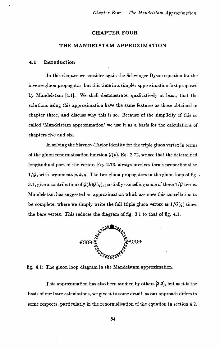
Chapter Four The Mandelstam Approximation
CHAPTER FOUR
THE MANDELSTAM APPROXIMATION
4.1 Introduction
In this chapter we consider again the Schwinger-Dyson equation for the
inverse gluon propagator, but this time in a simpler approximation first proposed
by Mandelstam [4.1]. We shall demonstrate, qualitatively at least, that the
solutions using this approximation have the same features as those obtained in
chapter three, and discuss why this is so. Because of tile simplicity of this so
called 'Mandelstam approximation' we use it as a basis for the calculations of
chapters five and six.
In solving the Slavnov-Taylor identity for the triple gluon vertex in terms
of the gluon renormalisation function 9(p), Eq. 2.72, we see that the determined
longitudinal part of the vertex, Eq. 2. 73, always involves terms proportional to
1/9, with arguments p, k, q. The two gluon propagators in the gluon loop of fig. -
3.1, give a contribution of 9(k )9( q), partially cancelling some of these 1/9 terms.
Mandelstam has suggested an approximation which assumes this cancellation to
be complete, where we simply write the full triple gluon vertex as 1/9(q) times
the bare vertex. This reduces the diagram of fig. 3.1 to that of fig. 4.1.
fig. 4.1: The gluon loop diagram in the Mandelstam approximation.
This approximation has also been studied by others [3.3), but as it is the
basis of our later calculations, we give it in some detail, as our approach differs in
some respects, particularly in the renormalisation of the equation in section 4.2. -
84

Chapter Four The M andelstam Approximation
As in chapter three we still neglect the ghost contributions and the diagrams
involving quartic gluon couplings. This allows our simplified equation to be
written diagrammatically as in fig. 4.2, giving us the following mathematical
equation for the inverse gluon propagator:
nf.lll n llll ~ c A95 J d4k r llOC( . k ) A (k)A' ( ) roP11
i'( -k,p, -q) ab = Oab + 0 ab 327r4 0 -p, 'q oP -y6 q 9( q)
(4.1)
where all the quantities are defined in sections 2.4 and 2.5, and once again we
work in the Landau gauge.
4.2 The Calulation and Renormalisation
Following Eq. 3.4 we write the integrand in Eq. 4.1 as 9(k )N"" jk2q2 ,
where we have explicitly extracted the simple functional dependence on 9 and
Nil" is defined as:
where:
Nf" = f~06 ( -p, k, q)bo~6.,.6rg"i'( -k,p, -q)
N:" = f~06 ( -p, k, q)k0 kpb7 6rg"i'( -k,p, -q)
Nf 11 = f~06 ( -p, k, q)bo~q7q6rg"7( -k,p, -q)
Nt" = f~06 ( -p, k, q)kok~q7q6rg"i'( -k,p, -q)
(4.2)
(4.3)
Using the form of the bare triple gluon vertex, as used in Eq. 3.10, some
simple tensor algebra gives:
85

Chapter Four The Mandelstam Approximation
II
I ......
I ......
fig. 4.2: The Schwinger-Dyson equation for the inverse gluon propagator using
the Mandelstam approximation.
86

Chapter Four The Mandelstam Approximation
Nt' =h'"'(p4 + k4- 2k2p2) + (2~~2- p2)pllpll + (2p2- k2)kllk"
-p. k(k 11 p" + p 11 k")
(4.4)
Projecting with the tensor P 1111 , Eq. 3.2, and denoting Ni = Nr" P1111
we obtain:
2 40 (k. p)2 10 2 NI =- 2p +- - -k ~ lOk. p
3 p2 3
(4.5)
We can now use the results of Appendix A to perform the angular
integrals to obtain:
87
Chapter Four The Mandelstam Approximation
(4.6)
where we have introduced an ultraviolet cutoff K2 making all the integrals in Eq.
4.6 finite. Putting all this together, dividing by p2 , and factoring out the colour
matrix 6ab, we obtain the following equation:
1
Q(p) - 1 + (4.7)
The beauty of this Mandelstam approximation is that it allows all the
angular integrals to be performed analytically, leaving us with just the momen
tum integration to do. This is to compared to the far more complicated situation
in chapter three. Thus Eq. 4.7 is a far easier equation to deal with numerically,
88
Chapter Four The Mandelstam Approximation
a feature which will be of essential importance when we come to consider the
coupled gluon and quark system in chapter six.
Because of the presence of the ultraviolet cutoff, we have really only de
fined 9(p, K ). As in chapter three we define a renormalised gluon renormalistaion
function by:
(4.8)
To obtain an equation independent of the cutoff K 2 , we first evaluate Eq. 4. 7 at
p2 = JL 2, where once again JL 2 is some arbitrary momentum~ We then subtract
this from Eq. 4.7, and use the definition in Eq. 4.8 to obtain a renormalised
equation:
(4.9)
where the kernel.J(k,p) is simply read off from Eq. 4.7. Here the renormalised
running coupling is given as:
(4.11)
and as usual a-1 (JL) = g2 (JL) / 47r. The subscript on the coupling a-1 (JL) is to dis
tinguish it from the couplings a 2(JL), aa(JL) defined from the quark-gluon vertex
which we will meet later in chapters five and six. The consistent renormalis-
tion of the Schwinger-Dyson equations is a highly non-trivial problem, which we
discuss further in chapt.er seven.
We must also mention the gluon mass renormalisation as in section
3.3 .. A term violating p2 /9(p) -+ 0, as p2 -+ 0 will arise from terms where
Q(p)"' AJL2 fp2 on the right hand side of Eq. 4.9 . This is equivalent to a gluon
mass term and must be subtracted. As in the previous chapter, the easiest way to
89

Chapter Four The M andelstam Approximation
deal "'ith such mass terms is to subtract the contribution where Q(p) = AJL2 jp2 •
Since the right hand side of Eq. 4.9 is linear in Q(k), the effect of this is to
completely cancel the contribution of such an infra-red enhanced term to the
integrals in Eq. 4.9. Such an enhanced term will, in general, give rise to infra
red divergent integrals (see section 3.3). However, because of the gluon mass
renormalisation this term does not appear on the right hand side of Eq. 4.9, and
thus no infra-red divergences arise. Thus if we write 9R(P) = AJL2 jp2 + 91 (p),
it is only the term 91 which will appear within our integrals.
4.3 The Solution
As in chapter three, it has not proved possible to find an analytic solu
tion to Eq. 4.9, and again we attempt a numerical solution. The analysis of the
possible low momentum behaviour of 9R(P) is similar to the dimensional anal-
ysis of section 3.4, so again we look for a solution with the enhanced infra-red
term, bearing in mind that the &luon mass renormalistaion above means that
this term does not contribute to the integrals we must perform. As in section
3.4 we can also extract the asymptotic form of 9 R(P) for large p2 • By expanding
9n = 1 + O(a1 (JL)), we easily obtain for the leading behaviour:
1 --9R(P)
(4.11)
where the final momentum integral can easily be performed to give "'16 = fCA.
Using Eq. 3.33, we can recast our definition of the running coupling in the form:
(4.12)
Again expanding in powers of a 1 (JL ), and using Eq. 4.11 we obtain:
(4.13)
90
Chapter Four The Mandelstam Approximation
where we easily see that f3b = 2'Yb = 134 C A from the simple form of E_q. 4.12.
The standard renormalisation group argument yields:
(4.14)
Since 'Y~/ /3~ = 1/2, we can use the usual one-loop asymptotic form for the
coupling arising from Eq. 4.13, to give us the asymptotic form for 9R(p)as:
1 (4.15)
Again we choose a parameterisation for 9 R(P) which reproduces this
asymptotic form, so we first introduce:
(4.16)
allowing us to parameterise 9 R(P) by:
(4.17)
where the parameters A, an, bn, Cn, dn, Pn and qn are allowed to vary. Since
all the angular integrals have been performed, we can allow the dimensionful
parameters Pn, qn to vary numerically. This is unlike the situation in chapter
three, where the corresponding dimensionful parameters were chosen by trial
and error. This was because of the large amount of computing time needed
when the parameters are allowed to vary under the integral sign, where only
one of the angular integrals can be performed numerically. Also, we expect a
non-zero value for the coefficient of the infra-red enhanced term A, but again
we do not prejudice this result, by allowing the possibility that this parameter
can be zero.
91

Chapter Four The Mandelstam Approximation
As before, we set 9R(J.t) = 1 and choose J.t 2 = 10 GeV2• We demand
consistent numerical agreement between input and output for the range 0.01 <
p2 < 100GeV2, with a 1 (J.t) = 0.15,0.2,0.25,0.3, i.e A1 = 159,335,525, 708MeV
respectively, where A1 is calculated using Eq. 1.23 with f3o = ~4 CA. In fact the
equation Eq. 4.9 has a momentum scale dependence which is wholly specified by
J.t, and by the value of the running coupling o 1 (p) at p2 = J.t2• As usual though,
this scale can be defined in terms of an intrinsic parameter of the theory, namely
A 1 • We find good agreement (to \'\-ithin 1%) with N,ll1 = 1 in Eq. 4.17. ·we
plot our results in fig. 4.3, and give the parameters obtained in table 4.1.
a(J.t) 0.15 0.2 0.25 0.3
A 0.004207 0.01533 0.03254 0.05263
al 0.9313 0.9352 0.9744 1.006
Po (GeV) 0.1794 0.3037 0.4501 0.6121
bl 1.055 0.9394 1.198 1.527
C} 0.1308 0.1386 0.1079 0.09592
qo (GeV) 0.1443 0.2636 0.3870 0.4867
dl 0.43i9 0.4918 0.6605 0.8051
Table 4.1 : Parameters for 9R(p), Eq. 4.9, for solutions shown in figs. 4.3.
Once again we obtain solutions which possess the infra-red enhancement
we saw in chapter three. Note that the size of this enhanced term rises with
A1 exactly as we would expect if A1 is the intrinsic momentum scale of the
theory. We discuss this further in chapter seven. In section 4.5 we will discuss
the physical implications of this enhancement of 9R(P) and hence the gluon
propagator, and see how it is related to confinement. Before this we first discuss
92

-C\l
~ ..._...... 0::
u
50
40
30
20
10
0 .01
Chapter Four The Mandelstam Approximation
input -
output •
. 1 1
fig 4.3: The gluon renormalisation function QR(P) in the Mandelstam approxi
mation, as a function of p2 , for a 1 (JL) = 0.15, 0.2, 0.25, 0.3.
93
10

Chapter Four The Mandelstam Approximation
the relationship between the Mandelstam approximation, and the full vertex
approximation of chapter three.
4.4 How Good is the Mandelstam Approximation?
In this and the preceding chapter, we have used two different approxi
mation schemes to solve the Sch"'inger-Dyson equation for the gluon propagator.
In both cases we have obtained solutions for the gluon renormalisation function
9n(p) which has an infra-red enhanced term AJI2 fp2 , which we believe to be in
dicative of confinement. In chapter three we solved the Slavnov-Taylor identity
for the triple gluon vertex in the absence of ghost contributions. This allows us
to write the longitudinal part of this vertex in terms of(}, where we drop the
subscript R for the discussion of this section. The solution for this longitudinal
part is proportional to 1/9 with arguments p, k and q. The propagators in the
gluon loop of fig. 3.1 contain a factor fJ(k)(}(q), and so we obtain three generic
terms, proportional to
fJ(~~~iq), fJ(k) and fJ(q) (4.18)
The last type can be made equal to the second type by the change of variable
k --+ q, q --+ k within the loop integral. The first term we denoted by C(k,p),
the second and third by JC(k,p), see Eq. 3.20. The Mandelstam approximation
assumes that the cancellation which occurs for the second and third tems in Eq.
4.18 occurs for the entire vertex.
An essential feature of both our calculations is the gluon mass renor
malisation, which subtracts off those terms on the right hand side of Eqs.
3.27 and 4.9, which do not vanish when we multiply by p2 and let p2 ~ 0.
Such contributions only arise from the infra-red enhanced term, so we write
(J(p) = AJI2 jp2 + (}1(p), and subtract from these equations the contribution
where any (} which appears in the numerator is put equal to its infra-red en-
94

Chapter Four The Mandelstam Approximation
hanced term only. This means that such singular terms do not contribute to
the right hand side of the Mandelstam approximation at all, and similarly not
in the X:( k, p) terms of the full vertex approximation. After this subtraction the
only singular terms which contribute to the .C(k,p) are those where one of the
factors of Q in the numerator is equal to AJL2 jk2, and the other is equal to Q1 •
For example:
(AJL2 jk2)QI (q)
Q(p) (4.19)
where the other contribution can be put in a similar form by a change of in
tegration variable. In section 3.5 we define the divergent contributions arising
from such a term by means of a plus prescription and the technical details are
described there. On dimensional grounds though, the integration must provide
a dimensionful quantity to balance the factor of JL 2 • Since the only variable
aYailable to us is p2 , after integrating such a quantity as in Eq. 4.19 we get a
contribution proportional to:
(4.20)
where W(p) is some function arising from the integration which is well behaved
as p2 -+ 0. In this limit the factor in the denominator also behaves like AJL2 fp2
and cancels with the term in the numerator. Thus the cancellation which occurs
completely in the Mandelstam equation, and partially for the X:(k,p) term in
the full vertex approximation before integration, is seen in a sense, to occur in
the infra-red limit of the equation for the .C(k,p) term after integration. Since
it is in this p2 -+ 0 limit in which using only the longitudinal part of the vertex,
and neglecting the transverse part is valid, we might expect that the simpler
Mandelstam equation will work. Of course the arguments above concern only
the qualitative analytic behaviour, and there is no reason why the Mandelstam
95

Chapter Four The Mandelstam Approximation
equation should not give quantitatively different results. By comparing fig. 4.3
with fig. 3.2 we see that this is indeed the case. However, as was mentioned in ref.
[3.2], although neglecting the transverse part of the triple gluon vertex will not
affect the existence of infra-red enhanced solutions, it will affect the coefficient of
such a term, and so we should not therefore worry about any further quantitative
difference induced by using the Mandelstam approximation.
Another difference between the two approximations lies in the different
renormalisations, and hence the different running couplings, Eq. 3.33 and Eq.
4.12. The important fact though, is the dependence of the running coupling on
Q(p), and in both cases we have:
(Q(p) )n
a(p) "' a_(J.t) Q(J.t) (4.21)
where n = 1 for the full vertex approximation and n = 2 for the Mandelstam
approximation. Although different, both couplings become strongly enhanced
at low p2, because of the factor of Q(p) in the numerator. This is exactly what
we would expect of the coupling in a confiDing theory, and in both cases this
enhancement is by a power law. In chapter seven we discuss other differences
between these couplings, and a later one which we shall meet in the inclusion of
quark loops in the gluon equation.
In summary, the cancellation of factors of Q used in the Mandelstam
equation is seen to arise in the full vertex approximation, partially before in
tegration, and partially after. The much simpler Mandelstam equation gives
rise to qualitatively similar solutions, both for the gluon renormalistaion func
tion Q(p) and for the running coupling. Since the Mandelstam equation is far
simpler to use, both analytically, and more importantly, numerically, it is this
approximation that we shall use in our studies of fermions in a non-Abelian
gauge theory in the subsequent chapters.
96

Chapter Four The Mandelstam Approximation
4.5 Confinement and a 1/p4 Gluon Propagator
In the studies of the Schwinger-Dyson equation for the gluon propaga
tor in this and the preceding chapter, we have demonstrated solutions for the
gluon renormalisation function Q(p) which are as singular as 1/p2 as p2 -+ 0.
This in turn means that the gluon propagator is as singular as 1/p4 • This same
behaviour has been found by others(3.2,3.3,4.2] in various different approxima
tions and truncations of these equations. It seems likely then, that this does
reflect the true behaviour of the gluon. Before we go on to study the inclusion
of coloured fermions in the theory, we first discuss ways in which this infra-red
enhanced gluon propagator is related to confinement.
Since we do not 'see' the gluon as a physical particle in the real world,
unlike the electron or photon, we cannot immediately translate this low energy,
or long distance, enhancement of its propagator directly into physical state
ments. Indeed, since the gluon propagator itself is not a gauge invariant quan
tity we should not expect this. Nevertheless, there is good reason to suggest
that this enhancement is physically meaningful, and related to the confinement
of colour. Here we shall discuss three ways in which to translate the behaviour
we have obtained for the propagator into statements about confinement. This
is not meant to be an exhaustive study of the implications of our solutions, but
they do contain good evidence that the infra-red behaviour we have obtained is
indeed a signal of confinement.
(i) The Static Colour Potential
In QED the long range force between two static electric charges is di
rectly related to the photon propagator(2.1]. By virtue of gauge invariance this
guarantees the Coulomb 1/r2 force law. The connection is based on considering
a 'one photon exchange' approximation, which for an Abelian theory correctly
gives the large distance limit. For QCD, because of the self coupling of the
97
Chapter Four The Mandelstam Approximation
gluon, this approximation breaks down[4.3], and we have to consider 'multi
gluon' exchanges between static colour charges as well. Nevertheless we present
here the 'one-gluon' exchange contribution to the large distance behaviour of
QCD, which gives us an intuitive feeling for the meaning of a propagator which
is as infra-red singular as 1/p4• Here we calculate a contribution to the large
distance potential between static colour charges. Because the gluon is a vector
particle, this one gluon exchange generates a vector contribution to the poten
tial. The multi-gluon exchanges we neglect will generate a scalar component to
the potential, and this is expected to play an important role[4.3].
The potential arising from one gluon exchange for a colour singlet state
is related to the propagator via:
V(r) = -CFg2 /_: dt ~oo(r, t) (4.22)
where ~00 is the time-time component of the full gluon propagator in configu-
ration space. Using its Fourier transform we obtain:
(4.23)
where z = (t,r) is the space-time variable. The t integral can be performed to
give a delta function of k0 , allowing the k0 integral to be performed trivially,
giving us:
V( ) C 2 J d3k A (k2) -ik·r
r = - F9 (21r)3 ~oo e (4.24)
where k, rare three-vectors. Using spherical polar coordinates we obtain:
V(r) = - CF~B roo k2 dk 11 dz r2fr d¢ ~oo(k2)e-ikrz 211" Jo -1 lo
(4.25)
where z = cos8. We perform the¢ and z integrals to give:
98

Chapter Four The M andelstam Approximation
V(r) 2CFeta100
• - - 3 wdwsmwtl.oo(w/r)
1rT 0 (4.26)
where w = kr.
Evaluating the gluon propagator at k0 = 0 gives us
(4.27)
and so our form for this one gluon exchange potential is:
V( ) 2CFet 8 100dw . 9(w/r) r = - sz nw ---'---'-...:..
1rr 0 w (4.28)
For QED we expect the photon renormalisation function to be approx
imately one. The potential can be easily calculated to be:
(4.29)
4r.r
where e1 , e2 are the electric charges of the two particles. This is the usual
Coulomb potential. For QCD, however, we have obtained a very different ba
haviour for 9(k), which we parameterise as Ap,2 /k 2 + 91 (k). The infra-red
enhanced term gives a contribution to the potential
(4.30)
where we have introduced a small momentum cutoff A to make the integral finite.
Using integration by parts twice, we can write the integral in Eq. 4.30 as:
sin(Ar) cos(Ar) 1100 dw. ----,-~~ + -- -sznw 2(Ar )2 2Ar 2 .>.r w
(4.31)
The integral in Eq. 4.31 is well behaved as A- 0, so we can expand Eq. 4.31
in powers of A giving:
99

Chapter Four The Mandelstam Approximation
roo dw sinw = ]_ - ~ l>.r w 3 Ar 4
{4.32)
The first term here gives a contribution to the potential which has no r de
pendence. Although it diverges in the limit A -+ 0 we can always subtract a
constant term from a potential, and so we remove this infinite constant, giving
us the enhanced contribution to the potential:
{4.33)
Thus our 1/p4 propagator generates a linear term to the static colour
potential. This linear potential is a good signal for confinement. In a Coulomb
potential the flux lines spread out radially to give a 1/r2 force law, for a linear
potential, they must be squeezed into a narrow 'flux tube' between the colour
charges. The energy needed to separate these charges grows linearly with their
separation. Eventually it will be energetically more favourable to create a qq
pair from the vacuum to shorten these stretched lines of flux. This process can
be repeated, until the momenta of the created quarks is low enough that they
form the bound states we call hadrons.
The Q1 (k2 ) contribution to the potential can be calculated numerically,
and the result for o:a(lt) = 0.25 is plotted in fig. 4.4. For comparison we plot
it against the phenomenological potential of Quigg and Rosner[4.4], which has
been succesful in describing the properties of heavy qq states, and is simply pa
rameterised as a sum of a linear term and a Coulomb 1/r term. From the nature
of our solution for Q, we see that this form for the potential arises naturally.
(ii) The Wilson Loop Operator
As we mentioned previously, this naive treatment of the propagator
to obtain the static colour potential does not give the whole answer for QCD.
Thus we cannot yet conclude that this potential does rise linearly with distance
100
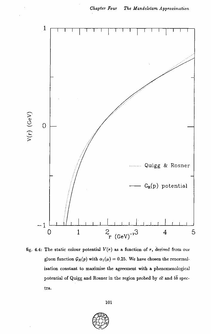
Chapter Four The Mandelstam Approximation
1
0
......... Quigg & Rosner
-- GR(P) potential
-1 0 1 4
fig. 4.4: The static colour potential V(r) as a function of r, derived from our
gluon function 9R(P) with a 1 (JL) = 0.25. We have chosen the renormal-
isation constant to maximise the agreement with a phenomenological
potential of Quigg and Rosner in the region probed by cc and bb spec-
tra.
101
5

Chapter Four The Mandelstam Approximation
for large separations. Indeed since the gluon propagator itself is not a gauge
invariant quantity, we should not expect to immediately be able to translate
its properties into physical statements. A quantity which is gauge invariant,
however, is the Wilson loop operator lV(L)[l.lO], defined by:
W(L) = jrnA]w(L)e-s j jrnAJe-s ( 4.34)
where [DA] denotes a functional integral over the gauge field, where we are
working in Euclidean space. Here we need the quantity w(L) defined by:
(4.35)
which is the integral of the gauge field around a closed loop L in space-time.
Here the symbol P denotes the path ordering of the A a matrices around the
loop, which were introduced in section 1.3. For rectangular loops, in which the
time distance is very long compared to the space distance, then the Wilson loop
operator is related to the static colour potential[l. 7] via:
W(L) = exp (- TV(r)) (4.36)
where T is the length of the time interval. For QCD to confine, it is supposed
that V(r) must behave linearly with r for large distances. Writing V(r) = ttr,
where we call tt the string tension, we would find in this case that
ll'(L) = exp (- ttAL) (4.37)
where AL is the area enclosed by the loop. This result generalises to any shape
of contour. Thus a possible criterion for confinement which is gauge invariant
would be that the Wilson loop obeyed a so-called 'area law' for large loops, i.e.
that this operator was exponentially damped, with the damping proportional
to the area enclosed by the loop. For a non-confining theory such as QED, we
102
Chapter Four The M andelstam Approximation
expect the potential to be constant at large distances, and thus the Wilson loop
will be exponentially damped only proportional to the perimeter length of the
loop.
The Wilson loop is a quantity that can be calculated on a space-time
lattice[l.lO], and indeed Creutz has shown an area law at least for a lattice SU(2)
theory in the strong coupling limit. It is hoped that lattice simulations of QCD
will themselves reveal an area-law, which will still hold in the continuum limit
of these lattice theories (see section 1.5).
An important result by West[4.5] relates the Wilson loop operator to
the full gluon propagator. The result. states that if in any gauge, the full gluon
propagator is as singular as 1/p4 as p2 -+ 0, then the Wilson. loop obeys an
area law. This is the result we need, relating our gauge variant propagator to
a gauge invariant quantity, which itself is related to the static potential. Some
comments are needed here. First of all, since we had to truncate the Sch·winger
Dyson equations in order to obtain a closed equation, we cannot yet prove that
the enhanced infra-red behaviour we have found is indeed the behaviour of the
exact propagator. Nevertheless, the link with our results and a linear confining
potential is suggestive. If we could show that this enhanced behaviour does
hold for the exact propagator, then it will have essentially been demonstrated
that QCD can indeed confine coloured objects. This would provide impressive
support for the perturbative successes of QCD.
There have been previous studies of the Schwinger-Dyson equation for
the gluon propagator, and it is appropriate here to mention the most important
of these, by Baker, Ball and Zachariasen[3.2]. Their study is in many ways sim
ilar to our.own, but with the crucial difference that they work in an axial gauge
instead of a covariant one. This has the bonus that all the ghost terms are ab
sent, greatly simplifying the equations themselves, as well as the Slavnov-Taylor
identities. The propagator itself, however, is more complicated, depending on
103

Chapter Four The Mandelstam Approximation
two scalar functions instead of just the one, namely Q, in our calculation. They
employ an approximation in which they assume that the dominant infra-red be
haviour is given by only one of these functions, so that their full propagator has
the tensor structure of the free one. They also assume that the coefficient of
any infra-red enhanced term is independent of the gauge chosen. Under these
assumptions the integrals involved in the truncated Schwinger-Dyson equation
for the propagator are infra-red finite, even in the presence of the enhanced
term. Unfortunately these approximations are put in somewhat by hand, and
as usual in axial gauges, there is still the problem of dealing with the spurious
singularities when one of the momenta in the problem becomes orthogonal to
the vector defining the particular axial gauge. A prescription for dealing with
these has also to be introduced 'by hand', and there is still controversy over how
to deal with them properly[4.6], even in perturbation theory.
The most compelling reason, however, for choosing to work in a covari
ant gauge is ·because of another important result by West[4.7]. Here he shows
that because all the particles appearing in axial gauges are physical ones (i.e.
no ghosts), that the spectral functions obey certain positivity conditions. The
important conclusion from this is that he finds it impossible for the full axial
gauge propagator have an infra-red behaviour more singular than 1/p2• Note
that this does not contradict the results of Baker, Ball and Zachariasen, in that
they only considered one of the two scalar functions appearing in the axial gauge
propagator. This may well indeed be as infra-red singular as 1/ p4 even though
the full propagator is not. Presumably this enhanced infra-red behaviour would
cancel between the two functions. This does, however, call into question their
approximation of only considering one of the functions. More importantly, we
must relate whatever behaviour we find for the propagator to physical, and hence
gauge invariant quantities. The conclusion of this 'no-go' theorem of West's, is
that it will be impossible to prove confinement via the Wilson loop in axial
104

Chapter Four The Mandelstam Approximation
gauges.
Fortunately this theorem does not hold in a covariant gauge, and does
not in anyway constrain the possible infra-red behaviour of the covariant gauge
propagator. In the light of the problems arising in axial gauges, this is a com
pelling reason for studying the Sch"inger-Dyson equations in a covariant gauge.
(iii) The QCD Vacuum and Dual Chromomagnetic Superconductivity
A different approach to the link between confinement and a 1/ p4 prop
agator is related to the ideas of superconductivity[4.8) and electromagnetic du
ality. This duality is the invariance of Maxwell's equations under the transfor-
mations:
E -+ B B -+ -E Pe -+ Po Po -+ Pe (4.38)
Here Pe,Po are the electric and magnetic charge densities respectively, and E
and B are the electric and magnetic field vectors.
First we consider the electromagnetic action in a source-free, transla
tionally invariant medium:
(4.39)
as usual F,.,.ll .= a,.,.AII- aliA,.,., and e(z- y) is the dielectric constant describing
the polarisation properties of the medium. For a free theory we have e( x - y) = 6(z - y) and Eq. 4.39 reduces to the usual Maxwell action. The action of Eq.
4.39 leads to the equations:
(4.40)
where:
105
Chapter Four The Mandelstam Approximation
- J 4 Gpv(x) = d Y€(x- y)Fpv(Y)
Fpv(x) = ~€pvpuFpu(x) ( 4.41)
The first of the equations of Eq. 4.40 is the equation of motion, whilst the
second is the Bianchi identity.
It is equally possible to formulate this theory in terms of magnetic, or
dual potentials Bw We introduce G"'" = 8"'B"- 8"'B". Then the action, Eq.
4.39, can be written:
(4.42)
where we call p,(x- y) the magnetic permeability, which satisfies:
J d4 y€(x-y)p,(y-z) = h(x-z) (4.43)
Using this new action Eq. 4.42, we have the equations:
(4.44)
where
Fpv(x) = J ~y p,(x- y)Gpv(Y)
Gpv(x) = ~€pvpuGPO'(x) (4.45)
where this time the second of Eq. 4.44 is the equation of motion and the first is
the Bianchi identity. The statement of duality, is the invariance if physics under
the transformation Fpv +-+ Gpv·
An electric source is best treated by adding a term J! A" to Eq. 4.39,
changing the first of Eq. 4.40 to 8,.,G,.," = J~. For a magnetic source we can
add a term J~ B" to Eq. 4.42 to change the second of Eq. 4.44 to 8"'F"'" = J~
106

Chapter Four The Mandelstam Approximation
The formulation preferred depends on the sources present and the properties of
the medium.
We can form the current:
( 4.46)
and the current correlation
(4.47)
Similarly we have the magnetic current correlation:
( 4.48)
These correlations are nothing more than inverse propagators. In momentum
space, the relation Eq. 4.43 between f and Jl becomes E(k2 )JL(P) = 1, with both
equal to unity for a free theory. Perturbatively we can write:
(4.49)
Since we know that electrically charged particles produce screening for the A 11
potential (i.e. QED), they must produce anti-screening for the B11 potentials.
The opposite will hold for magnetically charged particles or magnetic monopoles.
Thus the anti-screening observed in QCD can be ascribed to a 'monopole-like'
behaviour, and indeed this can be made somewhat more rigorous(4.9).
We now turn to a consideration of electrical superconductivity. This is a
fully non-perturbative phenomenon, with f and Jl very different from unity. The
most important manifestation of superconductivity is the exclusion of magnetic r
fields from inside the superconducting medium, suggesting JL(k2 ) = 0. In fact we
know that magnetic fields penetrate up to the London penetration depth >.L. So
for a finite >.1 we would have at small k2 that JL(k2) = k2 /mi,, where mL = 1/ >.L.
107

Chapter Four The Mandelstam Approximation
Using the fact that fJ.l = 1 we have that for small k2 that f( k2 ) = m jj k2 • Thus
for small momenta, using Eq. 4.47 the inverse photon propagator becomes
proportional to:
(4.50)
Thus the propagator behaves like 1/ m 1 for small momenta, and we see that
the photon has acquired a mass. It therefore only propagates over distances
comparable to the London length ,\L. On the other hand the inverse propagator
for the 'dual' photon, derived from the Bp. potentials, has a small momentum
behaviour given by:
(4.51)
Thus the dual photon propagator is as singular as 1/k4 in this limit.
Consider then the theoretical possibility of a 'magnetic superconductor',
where exactly the reverse happens. We would now have a massive dual photon,
with the photon itself as singular as 1/k4 at small momenta.
This result is suggestive, as this is precisely the momentum behaviour
we have found for the gluon at small momenta. For QCD though, this analysis
is complicated by the non-Abelian nature of the theory. Nevertheless, it is
still possible to define dual non-Abelian potentials[4.10], and it is expected that
the correlation between the behaviour of the gluon propagator and its dual
holds. Thus our result that the gluon propagator is as singular as 1/k4 at small
momenta can be interpreted as a signal that the QCD vacuum is behaving like
an infinite chromo-magnetic, or dual superconductor.
It is interesting to consider what would happen when we put magnetic
monopoles inside our ordinary electrical superconductor. Because of the Meiss
ner effect, a single monopole would not be able to exist, as it would take
108

Chapter Four The Mandelstam Approximation
infinite energy to place it inside our superconductor. With more than one
monopole, however, we would have the possibility of forming monopole-anti
monopole bound states, where the two particles would have a separation of the
order of the London penetration length or less. In a type I superconductor the
magnetic flux would be essentially contained within a small volume, whereas for
a type II superconductor the magnetic flux would be squeezed into a small tube,
with the monopole and the anti-monopole at the ends.
'''ith a dual or magnetic superconductor, it would be electric monopoles
which could not exist singly, but could form bound states with other electric
charges.
Thus we can now formulate a physically intuitive, albeit heuristic picture
of confinement. The QCD vacuum behaves like a chromo-magnetic supercon
ductor. Colour electric monopoles, such as quarks, cannot exist singly within
the vacuum but can form bound states with other quarks. There has been spec
ulation as to whether a type I chromo-magnetic superconductor corresponds to
a bag model of hadrons, whereas the type II version would correspond to flux
tube solutions. Indeed in a closer study of the dual formulation of QCD[4.10]
explicit flux-tube solutions have been constructed, displaying much of the be
haviour we might expect. A signal for this picture of confinement might well
be the 1/ k4 propagator that our investigation of the Schwinger-Dyson equations
has suggested.
109
Chapter Five The Fermion Equation
CHAPTER FIVE
THE FERMION EQUATION
5.1 Introduction
We now turn to the Sch"inger-Dyson equation for the inverse fermion
propagator in a non-Abelian gauge theory. In a similar manner to the deriva
tion of the gluon equation in section 2.4 we can derive an integral equation for
the quark propagator. Again we use the fact that the functional integral of a
derivative vanishes to obtain:
6S <-=- > +11(x) = 0
61/,(x)
Using Eq. 2.35 and the QCD Lagrangian Eq. 2.38, we obtain:
(5.1)
(5.2)
In terms of classical fields and connected Green's functions, we can write this
as:
Taking the derivative of Eq. 5.3 with respect to tPtJi(Y) and setting the
source terms and the classical fields to zero gives us:
110

Chapter Five The Fermion Equation
Now ihry/ht/J is equal to the inverse quark propagator from Eq. 2.35, and so we
obtain the equation depicted in fig. 5.1.
Our aim is .to solve this equation for the fermion renormalisation func
tion .F(p), see ref. [5.1] for previous studies of this equation. Of course, once
we have fermions in our theory we must include their effects in the pure gauge
sector, by considering closed fermion loops, which occur, for example, in the
gluon equation. As a first approximation, however, we can neglect these terms
in the so-called 'quenched' approximation. In this limit, the equation for the
inverse gluon propagator is that of a pure gauge theory. Thus we can take our
solution for Q(p) and use it whenever it occurs in the fermion equation.
The real world of course, contains the fermions we call quarks which
do couple to the gluons. In chapter six we will consider the equations for the
gluon and quark as a coupled system, fully including the dynamical effects of
the fermions in the gluon equation. As a first step towards this, the 'quenched'
approximation serves to outline the type of solutions we might expect in the full
theory, as well as setting up the machinery for the more involved study later.
5.2 The Ward Identity and the Equation for .F(p)
As in the discussion before Eq. 2.76, we write the full fermion propaga-
tor as:
(5.5)
Using this we can write the diagrammatic equation depicted in fig. 5.1 as:
s;.1 (p) = s;j.(p) - ;~~: j d4 k "( 11 SF(q)r"(k,q,p).6.""(k) (5.6)
Here SoF is the bare fermion propagator, i.e. Eq. (5.5) with .F(p) = 1, CF the
appropriate color factor, (Nb -1)/2Nc, and r''(k,q,p) is the full quark-gluon
vertex. As before q = p - k.
111

Chapter Five The Fermion Equation
II
I .....
I .....
fig. 5.1: The Schwinger-Dyson equation for the inverse fermion propagator in a
gauge theory.
112
Chapter Five The Fermion Equation
Once again it is the infra-red or low momentum behaviour we are inter-
ested in, and as demonstrated in section 2.3, it is the longitudinal part of the
vertex function r* which determines this. Once again we can use the Slavnov
Taylor identity for the quark-gluon vertex[2. 7] to determine this longitudinal
part. Neglecting ghost contributions as before, this reduces to the Ward iden
tity of an Abelian theory, Eq. 2. 75, which we solve for the longitudinal part,
give in Eq. 2.76. Using this, and the solution we obtained for the gluon func
tion Q(p) in chapter four, we can now derive a closed integral equation for the
fermion renormalisation function :F(p),
As an aside, we note that we have only included massless fermions. In
general, the mass is also a dynamical function of p2 , and its contribution to
the Ward identity of Eq. 2.75 can be determined [2.7]. Formally, however,
a solution to the Schwinger-Dyson equation in which this dynamical mass is
identically zero always exists, at least for vertex functions of the form of Eq.
2.76. However, there is the possibility of addressing the important question of
chiral symmetry breaking through these equations, and there have been some
studies in toy models [5.2], and in more realistic calculations [5.3]. Nevertheless,
to a good approximation, the non-generation of a dynamical mass should be a
valid approximation, at least for the first generation of quarks.
Returning to Eq. 5.7, we take its trace having first multiplied by p/4 to
obtain:
To perform the algebra, we writer~= r~ + rz, where:
113

Chapter Five The Fermion Equation
(5.9)
Defining:
(5.10)
Using the usual manipulations of spin algebra we first work out
'Yp.f'Y11 (k 2hP."- kP.k") = k2 -yP.f'Yp. -1f.1
= - 2k2f.- 2k. q1 + gk2 (5.11)
= - ~~~2 - 2k . q1 Multiplying by p/4 and taking the trace gives:
1 II(k,p) = 2( -q. pk2 - 2k. qk. p)
1 = 2( -p2k2 + k. pk2 - 2(k. p)2 + 2k2k. p) (5.12)
= !(3k2k. p- p2k2 - 2(k. p)2) 2
Next, defining
2I2(k,p) = ~Tr[JhP.f.(g + p)](q + p)"(k2hP."- kP.k") (5.13)
we first work out
=(I+ p)fi(f. + p)k2 -1f.Ci + p)(k · q + k · p)
= 2(q + p). qk2(g + p)- (q + p)2k2f. -1q2(k. q + k. p)
- ,p2(k. q + k. p) + k2p(k. q + k. p)
114
(5.14)
Chapter Five The Fermion Equation
Once again we multiply by p/ 4 and take the trace to obtain:
1 12(k,p) = 2[2(2p2 + k2 - 3k. p)k2(2p2 - k. p)- (2p- k)2k2(p2 - k. p)
+ (2k. p- k2)(k2p2 - 2p2k. p- k2k. p + 2(k. p)2)
. k4 p2 - k 2 (k · p)2 - 2k2p2(k · p) + 2(k · p)3- 2p2(k · P? + 2p4 k2
(5.15)
A useful way of writing 12(k,p) can easily be verified to be:
12(k,p) = (k2p2 - (!.·. p)2)(k2 - 2k. p + 2p2 )
= (k2p2- (k. p)2)(q2 + p2)
This allows us to write the equation for F(p) as:
1 F(p)
- 1-
(5.16)
where /1 (k,p) and l2(k,p) are given in Eqs. 5.12 and 5.16 respectively. This
equation, however, is in terms of bare quantities and contains divergences which
need to be renormalised, which we now proceed to do.
5.3 Renormalisation
As it stands Eq. 5.17 contains the usual logarithmic ultraviolet diver
gences as well as being potentially infra-red divergent as a result of the enhanced
low momentum behaviour of Q(p) we have discovered in the preceding chapters.
This equation is somewhat more complicated than that for the gluon we consid
ered in chapter four, as it involves both F and g, As usual, we make the equation
ultraviolet finite by introducing a running coupling. Before we do this, however,
we note the similarity of the structure of Eq. 5.17 to that of the gluon equation,
115

Chapter Five The Fermion Equation
Eq. 3.2i, we considered in chapter three. Generically we have two types of
terms, one set proportional to 9(k), the other proportional to 9(k):F(q)J:F(p).
As in section 3.3, there is a slight technicality with the terms in ! 2(k,p) because
of the factor 1/(q2 - p2). To deal with these we write 12(k,p) in the following
way:
12(k,p) = (q2 + p2)(J.~2p2- (k. p)2)
= (q2- p2)(J.~2p2- (k. p)2) + 2p2(k2p2- (k. p)2) (5.18)
In the first term the factor q2 - p2 cancels between the denominator and the
numerator. As in section 3.3 this split. is by no means unique, but once again, the
term we have added and subtracted contains less powers of k 2 in the numerator
and so is ultraviolet convergent.
We can now cast Eq. 5.18 in the following form:
1 g2CF J g5CF 1 J .14 - = 1- - 0
- d"kQ(J.~)K.(J.·,p)- ---- a-kQ(k)C(k,p) (5.19) F(p) 1Gr.4 161r4 F(p)
where
K.(k,p) = k4 \ 2 [11 (k,p) + k2p2- (k. p)2] qp
1 ( 2 2 )2] .C(k,p) = k4q2p2 F(q)[I1(k,p)- k p + (k. p
+ 2p2(k2p2 _ (k. p)2) [F(p)- F(q)]) q2- p"
(5.20)
At this stage, F(p) is formally F(p, K, >.), where >., K are infra-red and
ultraviolet cutoffs respectively, introduced to make the integrals in Eq. 5.19
finite. Infra-red divergences arise only from the enhanced 1/k2 term in9(k ), and
as we shall later show, only in the second integral of Eq. 5.19 involving C(k,p),
the other being infra-red finite.
To deal with the ultraviolet divergences, we introduce a running cou-
piing defined by:
116
Chapter Five The Fermion Equation
g2(p,) = g5Za("-/1-L) 1- ~~6~~ f d4 kK(k,p,)Q(k,tc)
( 5.21)
.where we introduce the renormalised functions 9n (as in section 4.2) and :Fr
specified by:
Za(tc/p,)9n(p) = Q(p,tc)
ZF(tcjp,,).jp,):Fr(p,).) = :F(p,A,tc) {5.22)
Note that since this definition only involves the K term, all the quantities in
in Eq. 5.21 are infra-red finite, and tlils coupling is well defined when ). -+ 0.
Using Eq. 5.19 we can also write this coupling as:
2( ) _ g5Za(tc/ p,)ZF(tc/ p,, ).j p,):Fr(/-L, A) g P, - g 2 CF
1 + ~ J d4 k Cr(k,p,)Q(k, tc) (5.23)
where Cr(k,p,) is the same as C(k,p,), but with :F replaced by :Fr in Eq. 5.17.
Inverting Eq. 5.21 gives:
Za(tc/p,) = _!__- CF J d4 kK(k,p,)Q(k,tc) (5.24) g2 (p,) 95 1671"4
Following the same procedure we used in Eqs. 3.28-3.33, we subtract Eq. 5.21
from itself evaluated at p, which gives:
Za(tc/p) = Za(tc/p,) _ CFZa(tc/p,) J ~kg (k)[K(k ) - K(k )) (5 25) g2 (p) g2 (p,) 1671"4 R 'p ' 1-L .
We now use Eq. 3.32, which simply derives from the definitions in Eq. 5.22 to
give:
1 9n(p,) ( 1 CF J 14 ( ))
92(p) = Qn(p) g2(p,)- 471" 3 a-k9n(k) K(k,p)- ~(k,p,) • (5.26)
Introducing o 2 (p,) = g2 (p,)/47r, we can expand Eq. 5.26 in powers of o 2 (p,) to
gtve:
117

Chapter Five The Fermion Equation
1 1 /3" p2
o:2(P) = o:2(JL) + 4; ln JL2 (5.27)
where /3~' = fCA + ~CF. The CA term comes from expanding the 1/9n(p),
using the result of Eq. 4.10. The CF term comes from the integral in Eq.
5.26 with 9n(k) = 1 + O(o:2 ), see Appendix A for the simple integrals needed
to calculate this. It is important to note that this coupling differs from o:1 (JL)
defined in chapter four. 'Ve postpone a discussion of this, and the consistency
of the renormalisations we have used until chapter seven.
Again we follow the manipulations of section 3.3, inverting Eqs. 5.21
and 5.23 in terms of the bare coupling g0 to give:
(5.28)
2 Z (K/ )ZF(Kj ,\f ) - . g2
(JL) 90 G JL JL, JL - :Fr(JL,A)- c~~:~ll) J d4 k9n(k).Cr(k,p)
Substituting these expressions in Eq. 5.19 gives after the usual rearrangement
the ultraviolet renormalised equation:
~~~:~~ = 1-02~;3CF [/ cJ4k9n(k)(K(k,p)- K(k,p))
+ J tf4k9n(k)(.Cr(k,p)- .Cr(k,p))] {5.29)
Before we proceed further, we must deal with the infra-red divergences
. which arise from the enhanced Ap2 jP term in the gluon renormalisation func
tion 9 n( k ). First of all, we determine the form of these divergences by setting
Qn(k) = Ap2 fk 2 in Eq. 5.26. The K:-term gives rise to an integral:
(5.30)
118

Chapter Five The Fermion Equation
Using the angular integrals in Appendix A, Eq. A.28, we find that this is equal
to:
(5.31)
This explicitly demonstrates that the infra-red divergent terms in the first of
these integrals cancel, leaving us "'-ith a finite contribution, as we mentioned
earlier. The Cr-term involves the following integral:
(5.32)
We split the range of integration into two regions (i) A2 < k2 < p2 and (ii)
p2 < k2• The infra-red divergences occur in the first of these regions, and we
extract the divergent terms explicitly by writing the term in square brackets in
Eq. 5.32 as:
[I1(k,p)- k2p2 + (k o p)2](Fr(q, A)- Fr(p, A))
+[II (k,p)- k2p2 + (k o p)2]Fr(p, A)
+2p2(k2p2 _ (k 0 p)2) [Fr(P, A;- ~r(q, A)+ .r;(p, A)] q -p
-2p2(k2p2 - (k 0 p)2)F;(p, A)
(5o33)
Here the prime denotes a derivative with respect to p2 o Essentially all we have
done is to add and subtract a term which cancels \1\--ith the integrand in the limit
k2 --+ 0, using the first term in a Taylor expansion of Fr. Thus the first and
third of the terms in Eqo 5o33 are infra-red finite, leaving us with the divergent
integral:
119
Chapter Five The Fermion Equation
1 d,4 k A~-t 2 [ 2 2 2
k4 2 -k2 (11 (k,p)- k P + (k · p) )Fr(p, .X) ).2<k2<p2 q
- 2p2(k2p2- (k. p)2)F;(p, .X)] (5.34)
Since the argument of Fr in Eq. 5.36 is p, the angular integrals can be performed
( see Appendix A) to give us:
2 1r2 [P 2 AJL 2 1 [ 3 ~~4 2 2 }).2 dk k2 k2 ( 2 p2 - 3k )Fr(p, .X)
2 I ( ) 2 1 k4
1 2)] - 2p Fr p, A (2k - 2 p2 - 2k (5.35)
The terms with a factor of k4 in the numerator are obviously finite, so we read
off the divergent terms as:
We can therefore write Eq. 5.29 in the symbolic form:
Fr(JL, .X) 1 [ )l .X] Fr(p,.X) = l+A(p,JL)+ Fr(p,.X) B(p,JL)+C(p,JL np_
(5.36)
(5.37)
Here the A(p, JL) term comes from the K-term which was infra-red finite. The
.C-term is divided into a finite piece B(p,JL) and a divergent piece, being ln(A/JL)
times C(p, JL ). The form of C(p, JL) is easily read off from Eqs. 5.3i and Eq.
5.29 to be:
C(p, JL) = _ 3o2<;;)CF [ Fr~, .X) + .r;(p; .X)_ Fr~' .X) _ .r;(JL, .X)] (5.38)
Note we have used the identity ln(p2 /A2 ) = ln(p2 jp2 )- 2ln(A/JL) in going from
Eq. 5.36 to Eq. 5.38, and included the lnp2 /JL2 term in B(p,JL). We have also
120

Chapter Five The Fermion Equation
included the infra-red finite terms from Eqs. 5.33 and 5.35 in B(p, 11 ). Both
A(p,11) and B(p,11) also include the contributions where we have used 91 (k) for
the gluon function, where as before we use 9R(P) = A11 2 fp2 + 91 (p). This term
has no infra-red enhancement, and so all the integrals "ill converge as A -+ 0.
Unlike the expression for C(p, 11 ), Eq. 5.38, no easy analytic form exists for
A(p, 11) and B(p, 11 ), and they are evaluated numerically on a computer.
Before we do this, however, we must make our equation infra-red finite
by eliminating the dependence on A. To do this we take Eq. 5.37 and evaluate
it at p2 = 11'2 • A can then be simply eliminated between the two equations to
give:
C(;, 11
) (:Fr(l1, A)-B(p, 11) - :Fr(P, A)(1 + A(p, 11 )) )
= C(l1\l1) (:Fr(I1,A)- B(11',11)- :Fr(I1',A)(1 + A(11',11)))
(5.39)
The term B(p,11) contains a factor :Fr in its integral definition from Eq. 5.29.
Thus the numerator of Eq. 5.39 is linear in :Fr, as is the denominator from Eq.
5.38. Thus we define a factor ZIR(A/11) such that:
(5.40)
where :FR(P) is the ultraviolet and infra-red finite fermion renormalisation func
tion. The factor Z 1 R( A/ 11) cancels between numerator and denominator, and
we can rewrite our renormalised equation as:
121

Chapter Five The Fermion Equation
It is important to mention that this way of dealing with the infra-red
divergences is different to the method employed in chapter three, where we
defined finite quantities by means of a 'plus' prescription. A fuller discussion
of this, and other features of the infra-red problems of these equations appears
in chapter seven. There is no contradiction with the calculations of chapter
three, however, since it is the gluon function determined by the Mandelstam
approximation in chapter four that we have used here. There any infra-red
divergences were removed by the gluon mass renormalisation, and the problem
did not arise.
Eq. 5.41 is a complicated equation to solve, but it is possible to simplify
it. Since the equation is invariant when we multiply :FR by a constant (this is
easiest seen from the form of the unrenormalised equation Eq. 5.19), we can
essentially see it as an equation for :FR(P)/:FR(J.l). Thus the value of :FR(J.l) is
not determined and we ·will later set it equal to 1. We can now rewrite Eq.
5.41, returning to the form of Eq. 5.38, but this time as an equation for the
finite function :F R(P ). The left hand side of this equation is a function of p and
independent of p,', whereas the right hand side is a function of p,' independent of
p. Hence each side must be equal to a constant which we write as ln6 / J.l· Thus
:F R(P) satisfies:
:FR(J.l) 1 [ . 6] :FR(P) = 1 + A(p,p,) + :FR(P) B(p,p,) + C(p,p,)lnp (5.42)
This is of course symbolically the same as Eq. 5.3i, but with the important
distinction that all quantities are well-defined when we let ..\ -+ 0.
In Eq. 5.41, :FR(J.l') is not an arbitrary number, in the sense that whilst
we are free to choose the momentum p,', the functional dependence of :F R(J.l')
on p,' is determined by the fact it is to be a solution of the Schwinger-Dyson
equation. Thus, in Eq. 5.42, 6 is a parameter to be determined. This was demon
strated explicitly by choosing a parameterisation for :FR (see section 5.4) and
122

Chapter Five The Fermion Equation
first solving Eq. 5.41 by varying the parameters until good numerical agreement
is obtained between the right and left hand sides. Then, taking our solution for
:FR(P) we can determine h through Eq. 5.42 for all values of p2 for which we nu
merically solved the equation. Over the range 0.01 < p2 < 100 Ge V2, we found
that lnh ·was constant within the numerical accuracy to which we worked. Solv
ing Eq. 5.42 directly, with lnh as a parameter is more efficient numerically, since
we determine h directly, rather than implicitly through Eq. 5.41. Of course,
once we have obtained a solution for :FR(P) the two approaches are identical.
Since we allow h to be determined, it can be seen as a dynamically
generated infra-red cut-off whose value, a priori, could be anything. Remarkably
we found h to be of the order of a few MeV. This is a momentum scale which does
arise in strong interactions and we discuss this further in chapter seven. That
the value is physically sensible, seems to justify the rather involved procedure
outlined above which makes the equation for the fermion function :F R(P) infra
red finite.
5.4 The Solution for :FR(P)
Just as in chapters three and four, an analytic solution to this equation
Eq. 5.42 is not possible, and again we attempt a numerical study. Before we do
this, we investigate the possible analytic form our parameterisation should take.
(i) H :F R(P) - p,2 I p2 as p2 -+ 0, then the left hand side behaves like p2 I p,2 in this
limit. The small momentum behaviour of the right hand side is dominated by
the enhanced J..t2 lk2 term in 9R(k ). On dimensional grounds we must balance
the p,2 in the numerator by a p2 in the denominator, and we see that agreement
is not possible.
(ii) H :FR(P)- constant as p2 -+ 0, then the left hand side will also behave like
a constant. As in (i) above, the right hand side gives a J..t2 IP2 behaviour, and
123

Chapter Five The Fermion Equation
again consistency is not possible.
(iii) Finally, if :F R (p) "' p2 /11 2 as p2 - 0, then the left hand side of Eq. 5.17
behaves like 112 /p2 , the same behavior we expect on dimensional grounds from
the right hand side. Thus in this case there is the possibility of a consistent
solution.
This rough analysis reveals the possibility of a solution for :FR(P) which
vanishes as p2 - 0. Note that we have not proven that the fermion equation
Eq. 5.42 does indeed demand this behaviour. It might be that it is impossible
to obtain a consistent solution over a range of values of p2 away from zero. In
order to demonstrate that this behaviour is indeed realised, we must investigate
the equation numerically.
In the asymptotic region for large p2 , we can expand :FR(P) = 1 +
O(a2),9R(P) = 1 + O(a2). As in the usual one-loop perturbative calculation of
the fermion self energy, :FR is finite. The l2(k,p) term vanishes to this order
because of the :FR(P)- :FR(q) factor (see Eq. 5.17), and the only contribution
comes from the 11 (k,p) term, Eq. 5.12, which with :F = 1 is identical to the
one-loop perturbative term (see section 2.6). Thus to O(a2) we have:
:F R - constant (5.43)
asymptotically. We therefore choose a parameterisation for :FR(P) which not
only vanishes as p2 - 0 but also reproduces the simple asymptotic form Eq.
5.43. We use
N f 2
:FR(P) = ?; p2 ~ r~
where fn, rn are parameters to be determined.
(5.44)
The use of such a form as in Eq. 5.44 seems to have prejudged the
vanishing of :F n(P) as p2 - 0. We argued above that this was the only possible
124
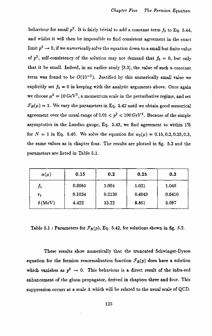
Chapter Five The Fermion Equation
beha·viour for small p2• It is fairly trivial to add a constant term fo to Eq. 5.44,
and whilst it will then be impossible to find consistent agreement in the exact
limit p2 -+ 0, if we numerically solve the equation down to a small but finite value
of p2, self-consistency of the solution may not demand that fo = 0, but only
that it be small. Indeed, in an earlier study [3.3), the value of such a constant
term was found to be 0(10-2 ). Justified by this numerically small value we
explicitly set fo = 0 in keeping with the analytic arguments above. Once again
we choose 112 = 10 GeV 2, a momentum scale in the perturbative regime, and set
FR(I1) = 1. \Ve vary the parameters in Eq. 5.42 until we obtain good numerical
agreement over the usual range of 0.01 < p2 < 100 GeV2 • Because of the simple
asymptotics in the Landau gauge, Eq. 5.43, we find agreement to within 1%
for N = 1 in Eq. 5.46. We solve the equation for a2(11) = 0.15,0.2,0.25,0.3,
the same values as in chapter four. The results are plotted in fig. 5.2 and the
parameters are listed in Table 5.1.
a(l1) 0.15 0.2 0.25 0.3
fi 0.9985 1.004 1.021 1.046
rl 0.1034 0.2130 0.4049 0.6410
6 (MeV) 4.422 13.22 8.861 5.087
Table 5.1 : Parameters for FR(p), Eq. 5.42, for solutions shown in fig. 5.2.
These results show numerically that the truncated Schwinger-Dyson
equation for the fermion renormalisation function FR(P) does have a solution
which vanishes as p2 -+ 0. This behaviour is a direct result of the infra-red
enhancement of the gluon propagator, derived in chapters three and four. This
suppression occurs at a scale A which will be related to the usual scale of QCD.
125

1.2
1
.8
.6
.4
.2
0 .01
Chapter Five The Fermion Equation
input -
output •
.1 1
fig. 5.2: The quark renormalisation function :FR(P) as a function of p2 , for
ll'2(JL) = 0.15, 0.2, 0.25, 0.3.
126
10

Chapter Five The Fermion Equation
For larger o 2 (p) we see that the suppression scale rises exactly as we would
expect from the dependence of the coupling on the intrinsic scale of the theory
(see sections 1.4 and chapter seven). For large p2 , Fn(p)"' 1 as in perturbation
theory, and the full fermion propagator behaves essentially like the bare one. If
this is taken as a model of the behaviour of the full quark propagator , we would
deduce that at large momenta they propagate as almost. free particles, just as
we see in high energy scattering, and as we would expect from the arguments of
'asymptotic freedom'. At low momenta, however, the propagation is suppressed,
and as p2 -+ 0 the suppression is sufficient that the quark propagator would van
ish, removing the particle pole on mass-shell at p2 = 0. This surely models the
features of a confining theory, answering the paradox of 'asymptotic freedom'
and 'infra-red slavery'. A more detailed discussion of all our results appears in
chapter seven.
1? ... _,

Chapter Six Quark Loops
CHAPTER SIX
QUARK LOOPS
6.1 Introduction
In the previous chapters we have obtained solutions for the quark and
gluon renormalisation functions Fn(p), 9n(p), which realistically model the qual
itative features we would expect of a confining theory. To date, however, we have
neglected the contribution of dynamical quarks by suppressing closed fermion
loops in the Schwinger-Dyson equation for the gluon. The relevant diagram
is depicted in fig. 6.1 with momentum labels. By neglecting this term in the
so-called 'quenched' approximation, the equation for the gluon decouples and
can be solved separately. The solution obtained can then be substituted in the
fermion equation. By including the contribution of closed fermion loops, there is
no decoupling, and we must try to solve the two equations simultaneously[6.1].
The validity of the 'quenched' approximation is based on the assumption that
the contribution of the added quark loop is small, and this would seem to be
borne out by the results of perturbation theory, where, for example the one-loop
beta function gives us:
11 2 f3o = -Nc- -n!
3 3 (6.1)
where Nc is the number of colours and n1 the number of light quark :flavours.
The naive counting given by this expression suggests that the effect of quarks
will be small.
There is other evidence [1.7], however, that in the non-perturbative
region quark loops play an important role. Indeed in a preliminary study of
the Schwinger-Dyson equations[6.2] the inclusion of quark loops has a marked
effect on the gluon renormalisation function. In that study, the contribution
of quark loops was calculated using the solutions obtained in the 'quenched'
128
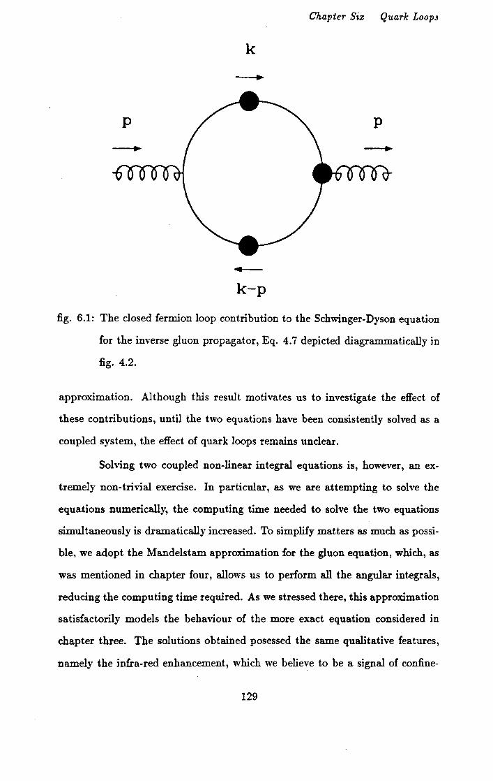
Chapter Six Quark Loops
k
k-p
fig. 6.1: The closed fernUon loop contribution to the Schwinger-Dyson equation
for the inverse gluon propagator, Eq. 4.i depicted diagrammatically in
fig. 4.2.
approximation. Although this result motivates us to investigate the effect of
these contributions, until the two equations have been consistently solved as a
coupled system, the effect of quark loops remains unclear.
Solving two coupled non-linear integral equations is, however, an ex
tremely non-trivial exercise. In particular, as we are attempting to solve the
equations numerically, the computing time needed to solve the two equations
simultaneously is dramatically increased. To simplify matters as much as possi
ble, we adopt the Mandelstam approximation for the gluon equation, which, as
was mentioned in chapter four, allows us to perform all the angular integrals,
reducing the computing time required. As we stressed there, this approximation
satisfactorily models the behaviour of the more exact equation considered in
chapter three. The solutions obtained posessed the same qualitative features,
namely the infra-red enhancement, which we believe to be a signal of confine-
129

Chapter Six Quark Loops
ment. Since both equations derived involve truncations and approximations,
we cannot hope to investigate quantitatively the low momentum properties of
QCD, but we can at least model its infra-red behaviour, and it is in this sense,
that it is valid to use the Mandelstam approximation.
6.2 The Quark Loop diagram
The first step in this study is to calculate the contribution of the diagram
shown in fig. 6.1, for one flavour of massless quark. We write its contribution
as:
As usual, the colour matrix .5ab has been factored out. Tp is the appropriate
colour trace, and we have a minus sign arising from the Feynman rules for
closed fermion loops. Note that since the fermion momenta are directed, we
have q = k - p. The other quantities are defined in chapters four and five.
In line with the calculation for the fermion equation in chapter five, we have
replaced the quark-gluon vertex with its longitudinal part, using the form Eq.
2. 76 for this, based on solving its Slavnov-Taylor identity in the absense of ghost
contributions, Eq. 2.i5.
As defined in Eq. 5.9 we write rL, = rr + 'r~ We therefore need to
evaluate two spin traces:
(6.3)
and
(6.4)
130

Chapter Six Quark Loops
We now contract this with the projection tensor pp.v, Eq. 3.2, giving the con
tribution of rr as:
(6.5)
and the contribution of r2 as:
(6.6)
We can now use the k-+ -q q-+ -k symmetry of the integral to write
Eq. 6.5 as:
g~TF J d4k ~ (8(k. p)2 - 2k2- 6k. ) 1671"4 k2q2 3 p2 p (6.7)
and to write Eq. 6.6 as :
(6.8)
As in the preceding chapters we must, in general, evaluate the expres
sions in Eqs. 6.7 and 6.8 numerically. However, since the fermion equation
remains explicitly unchanged, we will try to use the parameterisation in Eq.
5.45 for F(p), writing it as fip2 f(p2 + rf). For this simple form for Fall the
above integrals can be performed analytically. This only applies in the Landau
gauge, because of the simple asymptotic form of F. Of course, if we are un
able to solve the equations with this form for F, we would have to return to
Eqs. 6. 7 and 6.8, and perform a numerical integration with a more complicated
parameterisation for F(p).
131

Chapter Six Quark Loops
We first deal with Eq. 6.7. Using the integrals given in App~ndix A,
we can evaluate this as:
g5TF B1r2
[ 1P2
2 (8(p2 + k2
)k2
2k2 6k2p)
1611"4 3 o dk F(k) 8p4 - 2p2 - 4ps 2
1K ,2 • (8(p2 + ~~2)k2 2k2 6kp2)] + dk F(k) k4 - -k2- -ks p2 8. 2 4
(6.9)
where we have introduced an ultraviolet cutoff K. This simplifies to:
(6.10)
2
g5TF fi [ 1P dk2 k2
(k4
_ 3k2
)
611"2 o k2 + ri p4 p2
+ t dk' k' ~ r) ( - ::,) l (6.11)
Transforming variables to w 2 = k2 + ri gives:
g5TF fi [ 1P2+r~ dw2 ((w2- rns - ~ (w2- rn2) 611"2 r~ p4 w2 2 p2 w2
+ J.::;: ( -;:, ) l (6.12)
giving us the contribution of the rr term as:
(6.13)
The contribution of Eq. 6.8 is more complicated. First of all we use our
specific form for F(p) to obtain:
132
:F(q)- :F(k) k2- q2
There are three integrals to evaluate:
- ftr~
Chapter Six Quark Loops
(6.14)
(6.15)
Using the results of Appendix A, two of the angular integrals are trivial and
give a factor of 47r. The remaining angular integral can be performed using Eq.
A.21, with a= p2 + k2 + r~, b = 2pk, to give:
(6.16)
Although the momentum integral left is tractable, it is difficult and messy (see
ref. 6.2), and it is best performed using an algebraic manipulations program,
such as MACSYMA, which gives the results below:
133

Chapter Six Quark Loops
(6.17)
Where we have ignored terms of 0(1/ K 2 ). This gives the contribution of Eq.
6.8 as:
(6.18)
Note that because of the factor F(k)- F(q), the fact that F(k),F(q)- / 1 as
k 2 - oo, makes this term ultraviolet finite which is explicitly demonstrated in
Eq. 6.18.
Putting together Eqs. 6.13 and 6.18 and dividing by p2 gives the con
tribution of the fermion loop diagram as:
134

Chapter Six Quark Loops
(6.19)
For convenience we write Eq. 6.18 as:
n - !I g'5 Tp [Q( 2 2) -In( "'2 )] F - 1211"2 p 'rl rf (6.20)
where Q(p2 , ri) is simply read off. Note that llp is well behaved in the limits
p2 -+ 0, ri -+ O, as it should be from its integral definition. This term also makes
no contribution to the gluon mass (see sections 3.3 and 4.2), as it vanishes when
we multiply by p2 and take the limit p2 -+ 0. Note that Eq. 6.19 has the correct
one-loop perturbative logarithmic divergence.
6.3 The Gluon Equation with Quarks
We now return to the gluon equation derived in chapter four, where we
used the Mandelstam approximation for the triple gluon vertex. The unrenor
malised equation (Eq. 4. 7) can be written as:
(6.21)
where !:(p) is simply read off from Eq. 4.7. The inclusion of quark loops means
that the gluon equation becomes:
(6.22)
135

Chapter Six Quark Loops
where we have included n J flavours of massless quarks. As usual this really only
defines 9(p, ") and :F(p, A, K ), and we define the renormalised functions ( see
Eqs. 4.8,5.21 and 5.39) as:
ZG( K/ J-l )9 R(P) =9(p, K)
ZF(K/ J-L, A/ J-L)Zin(A/ J-L):Fn(p) =:F(p, A, K) (6.23)
As in section 4.2, we subtract Eq. 6.22 evaluated at p2 = J-l 2 from itself,
and, using the definitions in Eq. 6.23, we obtain the renormalised equation
which includes quark loops as:
(6.24)
As in chapter four, o 1 {J-L) = Zb( K / J-l )g5/4Tr, and here the new coupling o3 (J-L) is
defined by oa(,u) = ZG( K/ ,u)ZF(K/ J-l, )..j J-l )Zin(>..j J-l )g5/4Tr These couplings are
different from each other and from the coupling o 2 (J-L) defined in chapter five ..
These differences are discussed in chapter seven. To solve our coupled set of
equations we choose to set o1 {~-t) = o2(J-l) = oa(J-l) = o(J-L).
We have two non-linear coupled integral equations involving the two un-
known functions 9R(p),:Fn(p), with all other quantites being specified. Dealing
with both equations simultaneously is a cumbersome numerical exercise, and so
we choose to adopt an iterative approach. Firstly, with n 1 = 0 the gluon equa
tion decouples, and the solutions obtained in chapter four for the gluon function,
and chapter five for the fermion function satisfy the coupled system identically.
For non-zero n1 we take our solution for :FR(P) with n1 = 0 and substitute
the values of the parameters obtained into Eq. 6.24. Keeping these fermion
parameters fixed, we then re-solve the gluon equation until we once again ob
tain consistent numerical agreement over our range of p2 • This new solution for
136
Chapter Six Quark Loops
YR(P) is then substituted into the fermion equation Eq. 5.41, and this too is re
solved until we find a new solution for :FR(P). This procedure is repeated until
the solutions we obtain remain reasonably stable. Having found these iterative
solutions for :FR(P) and YR(p), we now solve the equations as a simultaneous
pair allowing all the parameters to vary. This final step was not found to change
the iterative solutions very much, but did allow some 'fine-tuning'. Since the it
erative solutions were numerically close to the solutions which solve the coupled
set, the potentially difficult numerical excercise was much simplified.
So long as nf, the number of massless quark flavours was varied in
small steps, this iterative procedure was found to converge relatively quickly.
Using this method we obtain solutions for the coupled system for a(J.L) -
0.15, 0.2, 0.25, 0.3 as before. \Ve varied the number of flavours through n 1 -
0, 2, 4, 6 over the usual range of p2, 0.01 < p2 < 100 GeV2
• We plot the solutions
in figs. 6.2-6.9, and table the parameters in tables 6.1-6.4.
As in chapter four, we obtain solutions for the gluon renormalisation
function YR(P) which have the power-law infra-red enhancement term AJ.L2 fp2 •
This in turn is reflected in the suppression of the fermion renormalisation func
tion :F R(P ), to the extent that the particle pole at p2 = 0 is removed. The effect
of closed quark loops, however, is to dampen both these effects by quite a large
amount, as can be seen from figs. 6.2-6.9. Thus it is suspected that with more
than seven flavours of massless quarks, the enhancement of the gluon propaga
tor would no longer occur. This in turn would remove the suppression of the
fermion propagator, and we can see this as an aspect of 'deconfinement'. We
discuss this further in the next chapter.
Finally, in the same spirit of the discussion of the static colour potential
in section 4.5, we plot this for a(p,) = 0.25 with n 1 = 0, 2 in fig. 6.10. Again,
this is not to be taken too seriously, but merely demonstrates the 'deconfining'
effect of even a small number of massless quarks.
137

6
4
2
0 .01
Chapter Six Quark Loops
input
output •
fig. 6.2: The gluon renormalisation function 9 R(P) as a function of p2 for a(p.) =
0.15, with n1 = 0,2,4.
138

1.2
1
.8
.6
.4
.2
0 .01
Chapter Six Quark Loops
input
output •
fig. 6.3: The quark renormalisation function :F R(P) as a function of p2 for a(Jl) =
0.15, with n 1 = 0, 2, 4.
139

15
10
5
0 .01
6
Chapter Six Quark Loops
input
output •
fig. 6.4: The gluon renormalisation function g R(P) as a function of p2 for a(Jl) =
0.2, with n f = O, 2, 4, 6.
140
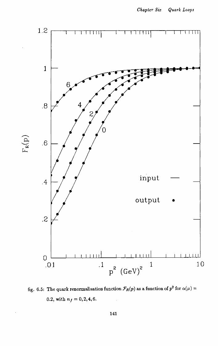
1.2
1
.8
.6
.4
.2
0 .01
Chapter Six Quark Loops
input
output •
fig. 6.5: The quark renormalisation function :FR(P) as a function of p2 for a(Jl) =
0.2, with n 1 = 0, 2, 4, 6.
141

30
20
10
0 .01
Chapter Six Quark Loops
·input
output •
1
fig. 6.6: The gluon renormalisation function 9 n(P) as a function of p2 for a(J.L) =
0.25, with n 1 = 0, 2, 4, 6.
142
10

1.2
1
.8
.6
.4
.2
0 .01
Chapter Six Quark Loops
6
input
output •
1
fig. 6. 7: The quark renormalisation function :FR(P) as a function of p2 for a(Jl) =
0.25, with n 1 = 0, 2, 4, 6.
143
10
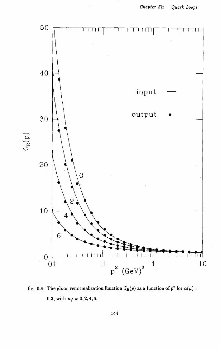
..-.. 0.. ....__,. a::
CJ
50
40
30
20
10
0 .01
Chapter Six Quark Loops
input
output •
6
1
fig. 6.8: The gluon renormalisation function g R(P) as a function of p2 for a:(f-L) =
0.3, with n f = 0, 2, 4, 6.
144
10
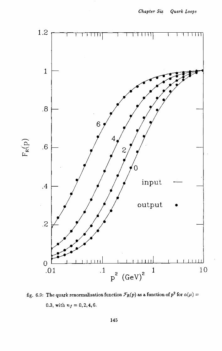
1.2
1
.8
.6
.4
.2
0 .01
Chapter Si:t; Quark Loop3
input
output •
fig. 6.9: The quark renormalisation function FR(P) as a function of p2 for a:(J.L) =
0.3, with n f = 0, 2, 4, 6.
145
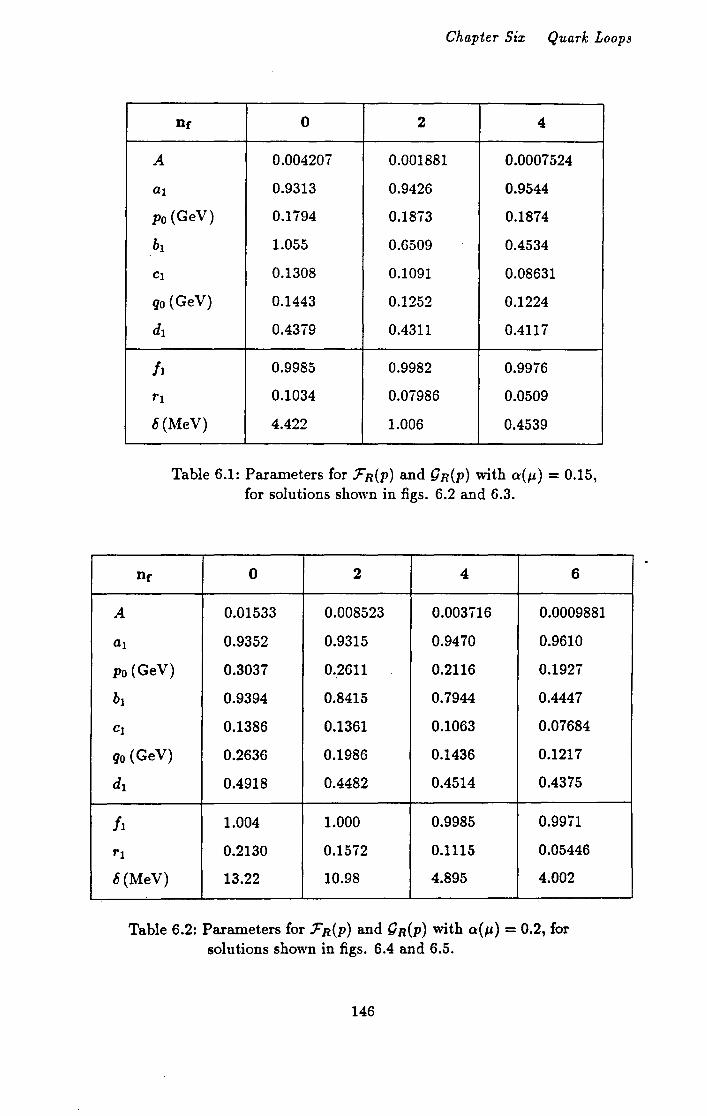
A
al
Chapter Six Quark Loops
Df' 0 2 4
A 0.004207 0.001881 0.0007524
a1 0.9313 0.9426 0.9544
Po (GeV) 0.1794 0.1873 0.1874
bl 1.055 0.6509 0.4534
CI 0.1308 0.1091 0.08631
qo (GeV) 0.1443 0.1252 0.1224
dl 0.4379 0.4311 0.4117
/I 0.9985 0.9982 0.9976
rl 0.1034 0.07986 0.0509
c5 (MeV) 4.422 1.006 0.4539
Table 6.1: Parameters for :Fn(p) and 9n(p) with a(J.t) = 0.15, for solutions shown in figs. 6.2 and 6.3.
nr 0 2 4 6
0.01533 0.008523 0.003716 0.0009881
0.9352 0.9315 0.9470 0.9610
Po (GeV) 0.3037 0.2611 0.2116 0.1927
bl 0.9394 0.8415 0.7944 0.4447
CI 0.1386 0.1361 0.1063 0.07684
qo (GeV) 0.2636 0.1986 0.1436 0.1217
dl 0.4918 0.4482 0.4514 0.4375
fi 1.004 1.000 0.9985 0.99il
rl 0.2130 0.1572 0.1115 0.05446
c5 (MeV) 13.22 10.98 4.895 4.002
Table 6.2: Parameters for :Fn(p) and 9n(p) with a(J.t) = 0.2, for solutions shown in figs. 6.4 and 6.5.
146

Chapter Six Quark Loops
nr 0 2 4 6
A 0.03254 0.0208 0.01046 0.003833
al 0.9744 0.9761 0.9467 0.9454
Po (GeV) 0.4501 0.4524 0.3935 0.4120
bl 1.198 1.296 1.128 0.4215
CJ 0.1079 0.1155 0.1299 0.1054
q0 (GeV) 0.3870 0.3250 0.2441 0.1696
dl 0.6605 0.6195 0.5188 0.4620
!I 1.021 1.010 1.001 0.9972
rl 0.4049 0.2980 0.1998 0.1167
6(MeV) 8.861 12.44 12.39 10.27
Table 6.3: Parameters for :Fn(p) and 9n(p) "'ith a(J.L) = 0.25, for solutions shown in figs. 6.6 and 6.7.
nr 0 2 4 6
A 0.05263 0.03758 0.02173 0.009141
al 1.006 0.9778 0.9605 0.9843
Po (GeV) 0.6121 0.6046 0.8482 0.6095
bl 1.527 1.432 0.5433 0.1634
CJ 0.09592 0.1226 0.1269 0.06521
q0 (GeV) 0.4867 0.4498 0.3827 0.3066
dl 0.8051 0.7034 0.5990 0.5852
!I 1.046 1.029 1.015 1.001
rl 0.6410 0.5035 0.3512 0.2103
6 (MeV) 5.087 7.769 10.90 12.47
Table 6.4: Parameters for :Fn(p) and 9n(p) with a{J.L) = 0.3, for solutions shown in figs. 6.8 and 6.9.
147

Chapter Six Quark Loops
1
-> Q)
l.? 0
-- n 1=0
········· Tit=2
-1 0 1 2 ( )-13 r GeV
4
fig. 6.10: The static colour potential V(r) as a function of r, derived from our
gluon renormalisation function 9R(P) for a(Jl) = 0.25, with n 1 = 0, 2.
148
5

Chapter Seven A Non-perturbative Study of QCD
CHAPTER SEVEN
A NON-PERTURBATIVE STUDY OF QCD
7.1 Propagation of Quarks and Gluons
In the preceding chapters we have used a truncation of the Schwinger
Dyson equations to investigate the infra-red behaviour of the quark and gluon
propagators in QCD. Our numerical analysis of the gluon and quark renormal
isation functions VR(p), FR(P) reveal a striking low momentum behaviour. In
the_ two different approximations we have used for the gluon equation in chap
ters three and four, we have obtained a consistent solution for VR(P) which is
as singular -as 1/p2 as p2 --. 0. This means that in this infra-red limit the gluon
propagator itself is as singular as 1/p4 • As discussed in section 4.5, there is very
good reason to suppose that this enhanced infra-red behaviour is an indication of
confinement. This can be demonstrated in a gauge invariant way by the fact that
the Wilson loop operator obeys an area law. More naively, the Fourier transform
of the propagator, which will contribute to the potential between static colour
charges, gives rise to a linear term which should be sufficient to confine colour.
We also have a simple intuitive interpretation of this confinement mechanism,
it being related to a 'dual' Meissner effect with respect to colour charge.
We then proceeded to investigate the effect that this infra-red enhance
ment of the gluon has on the propagation of the coloured quarks. Corresponding
to the low momentum enhancement of the gluon we find a suppression in the
fermion function FR(p), such that it vanishes at p2 --. 0. Indeed it vanishes
sufficiently fast that ~here is no physical particle pole on the quark mass-shell at
p2 = 0. Physically we can say that a quark cannot propagate on, or near mass
shell, because of the vanishing of its propagator. At high momentum, however,
the propagator is found to behave as if it were almost free. This offers us an
explanation perhaps, of the experimental observation of almost free quarks in
149
Chapter Seven A Non-perturbative Study of QCD
high energy collisions over small distances, before the confining mechanism sets
in as the quarks separate to larger distances. This high energy behaviour is also
found for the gluon propagator. This is exactly what we would expect from the
successes of perturbative QCD at high energies, and in particular the property
of 'asymptotic freedom'.
As was also mentioned in section 4.5, we have chosen to work in a
covariant gauge as opposed to an axial gauge which has been studied before. This
was a necessary step, as this infra-red enhancement which seems so intimately
related to confinement can be shown to be absent in an axial gauge, and we
cannot therefore hope to demonstrate confinement by using the Wilson loop
operator in such axial gauges. Since this particular argument relies on gauge
invariant quantities it remains the most important way of extracting information
about the theory from the non gauge invariant propagator.
We have managed to demonstrate the validity of the simple 'Mandel
starn approximation', used in chapter four, by comparing the qualitative features
of the results obtained, to the more exact approximation used in chapter three,
based on solving the Slavnov-Taylor identity for the full triple gluon vertex. Be
cause of its relative simplicity, the use of the Mandelstam approximation has
allowed us to study the inclusion of massless quarks into the theory. Numerical
simplicity was essential in studying the coupled equations for both the quark
and gluon propagators in chapter six, which is the first study of a dynamically
coupled quark-gluon system within the context of the Schwinger-Dyson equa
tions.
The infra-red enhancement of the gluon propagator, and the correspond
ing suppression of that of the quark, was first studied using the 'quenched'
approximation, in which the effect of closed quark loops was neglected in the
equation for the gluon. This infra-red behaviour was found to survive the inclu
sion of dynamical quarks, and the subsequent coupling of the equations. We do
150

Chapter Seven A Non-perturbative Study of QCD
find, however, that the effects are damped, and that as we include more-flavours
of fermions the gluon propagator has much less enhancement, and as a result of
this, the suppression of the quark propagator is diminished. Indeed, as can be
seen from the graphs in figs. 6.2-6.9, it seems that for about eight flavours of
massless quarks the enhancement of the gluon propagator, and therefore maybe
confinement, ·will disappear. We might well expect this, for the inclusion of
quarks affects the one-loop beta function in perturbation theory (see Eqs. 1.17
to 1.23) to the extent that for more than sixteen flavours of quarks the sign
of {30 will change. This will mean that to leading order in perturbation the
ory the coupling strength will behave like that of QED, and grow as we go to
larger momentum, becoming smaller as we go to low momentum. The effect
that we find, however, suggests that non-perturbatively quarks have a bigger
effect than we might naively expect from perturbation theory. Although it is
only the qualitative features of our study which are likely to be reliable, this
conclusion does support other evidence[6.2,6.3] that quarks play an important
role in non-perturbative physics.
7.2 Ultraviolet Problems
In order to solve the equations generated for the quark and gluon prop-
agators, it was necessary to remove the ultraviolet divergences which occurred,
and to introduce the running couplings 0'1 (i-t), a2 (JL ), 0'3 (JL) from Eqs. 4.12,5.26
and 6.23, which for completeness we give here:
_1_· __ 1_(QR(IL)) 2
0'1 (p) - 0'1 (JL) 9R(P)
_1_ = 9R(JL) (-1-- Cp J trkQR(k) [JC(k,p)- JC(k,JL)l) (i.1) a2(p) 9R(P) a2(1l) 47r3
1 _ _ 1_QR(JL) :FR(IL) as(p) as(JL) 9R(P) :FR(P)
151

Chapter Seven A Non-perturbative Study of QCD
The last of these is derived in an analagous way to the first two using the
definition of o:a(J.l) follo"'-ing Eq. 6.22. The consistent renormalisation of the
Schwinger-Dyson equations is as yet an unsolved problem. Exact gauge invari
ance, as expressed in the content of the Slavnov-Taylor identities demands that
these three couplings should be the same[1.6,2.1]. This is patently not so, as we
can see from Eq. 7.1, but we would expect this, as the truncation detailed in
chapter two, used to derive the equations we have studied, ignores the Schwinger-
Dyson equations for the three-point functions. It is these that determine the
behaviour of the couplings in the theory.
In our equations it is only the explicit O:i(J.l) that appear, although of
course the full running coupling does enter implicitly through Eq. 7.1, and the
equations for 9R(P) and :FR(p).
We can expand Eq. 7.1 in powers of the O:i to obtain:
(7.2)
where we have distinguished the three Ai (see sections 1.4 and 3.4). The coeffi
cients p~i) are equal to :
(7.3)
where we have included the effects of fermions in 0:1 (J.l ), and used the fact that
:FR(P) is finite to one-loop in the Landau gauge. The lowest order perturbative
results in the Landau gauge: /10 = (11/3)CA -(4/3)nJTF, which is independent
of the gauge, and "Yo = (13/6)CA - (4/3)nJTF are both independent of the
Casimir CF as a result of gauge invariance. Eq. 7.3 highlights the differences
between our three couplings. We note in passing that all three couplings have
152

Chapter Seven A Non-perturbative Study of QCD
the correct sign for /30 , as they better had do if we are to control the asymptotics.
For completeness we plot the three running couplings in fig. 7.1, over
the range of p2 for which we solved the Schwinger-Dyson equations for 9R(P)
and :FR(p). Outside this range we cannot consistently determine them from
Eq. 7.1 because of the dependence on these quark and gluon renormalisation
functions. In the light of this it should be mentioned that for small enough
p2, the a 2(p) coupling develops a pole. This arises from the bracketed term
in the second equation of Eq. 7.1. The enhanced term AJ.L2 jk 2 from 9R(k)
inside the integral does not generate any infra-red singularities (see section 5.3).
Nevertheless, it generates a term proportional to J.L 2 jp2 by dimensional counting,
which for sufficiently small p2 (outside our range) is large enough to cancel
the term 1/o:2(J.L). Hence 1/a2 (p) is zero and the coupling has a pole. This
behaviour though, is entirely due to the form of our renormalisation, and to
the approximations we have used. A totally consistent renormalisation of the
equations which properly treats the couplings should rectify this problem. The
other two couplings are well behaved for all momenta. In our study we make
the simple ansatz that 0:1 (J.L) = 0:2 (J.L) = o:a (J.L ).
In previous investigations of the Schwinger-Dyson equations, there has
been little or no discussion of the problems of a consistent renormalisation. This
remains one of the outstanding problems in using these equations to investigate
non-perturbative physics. Hopefully by highlighting the difficulties as we have
done here, it will be possible to reach a greater understanding of the problems
involved, and eventually to solve them.
On a practical level, we note that not only do the ultraviolet renormal-
. isations we have employed serve to make our equations finite, but they have
done so independently of any form of parameterisation we might choose for the
functions YR(P) and :FR(p). Since our study has been largely a numerical one,
the particular solutions we obtain should hopefully be numerically similar to the
153

.......-... ~ .._..,
...... c:s {fJ
~ ...,._..)
till ~ Q) ~
...,._..)
if)
till ~ .,......,
......... ~ ;j 0 u
5
4
3
2
1
0 .01
Chapter Seven A Non-perturbative Study of QCD
a1(p)
.1 10 100
fig. 7.1: The three running couplings ai(JL), with i = 1,2,3, as a function of p2,
with ai(JL) ~ 0.2, i = 1, 2, 3.
154
Chapter Seven A Non-perturbative Study of QCD
exact solutions, although the analytic form will certainly be different.
Finally it is of interest to ask how the solutions depend on the renor
malisation scale p 2 • Were our renormalisations entirely consistent, we would
expect them to be invariant under the transformations of the renormalisation
group (see section 1.4). Since our renormalisations are not totally consistent
we might expect some discrepancy. Nevertheless, it is possible to show that
our solutions are at least approximately renormalisation group invariant. To
demonstrate this we return to the Mandelstam equation of chapter four, ·with
no quarks for simplicity. We start from Eq. 4.12, which we cast into the form:
(7.4)
where here we use the notation (} R(P, Jl) to denote the gluon renormalisation
function evaluated at p2 , with renormalisation scale p 2 • We can evaluate this
equation at a different renormalisation scale 712• Since we must have (} R (JL, Jl) =
YR(71,Ji) (which we usually choose equal to 1), we can easily derive:
- ( 0'1 (JL)) 1/2 YR(p, Jl) = 9n(p, Jl) a
1 (71
) (7.5)
YR(p,p) -
(} R(71, Jl)
We can re-solve our Schwinger-Dyson equation, but this time choosing a
renormalisation scale "ji2 • The equation now depends explicitly on a 1 (71), which
we can evaluate from the first equation in Eq. 7.1 (see fig. 7.1), using our
previous solution for the Schwinger-Dyson equation plotted in fig. 4.3. Having
done this, we can check to what extent Eq. 7.5 holds. We solve the equation
for three scales: p 2 = 4, 10,25 GeV2 , where we choose a 1 (10) = 0.2, which
gives us a(4) = 0.2558 and a(25) = 0.1650 (see fig. 7.1). Here we use an
obvious notation, in that a 1(4) denotes the value of the running coupling ai(P)
at p2 = 4. From the solution of chapter four (parameters in table 4.1), we
155

Chapter Seven A Non-perturbative Study of QCD
have 9R(4, 10) = 1.131, 9R(10, 10) = 1 and 9R(25, 10) = 0.9083. The curves
9R(P, J.L) x 9R(J.L, 10) are plotted for our three different values of J.L 2 in fig. 7.2.
We see that Eq. 7.5 does indeed hold to l'\rithin a satisfactory degree.
This completes our discussion of the ultraviolet renormalisation of the
equations we have studied. It is evident that problems of consistency remain
and that further research is required. However, in the spirit of this study as a
model for the true behaviour of these equations, it is hoped that what we have
achieved does shed some light upon the non-perturbative region of QCD, as well
as highlighting the problems which further study must face.
7.3 Infra-red Problems
Central to the results obtained throughout this study, is the conclusion
that as the momentum y - 0, the gluon renormalisation function 9R(P) "'
AJ.L 2 lp2 , and hence the gluon propagator -behaves like 1lp4 in this limit. The
size of this enhancement AJ.L2 carries the dimensions of mass-squared, and is
presumably related to some intrinsic scale of the theory A. This enhancement
of the gluon leads to;a suppression of the quark function FR(p), which using the
parameterisation of Eq. 5.44 is characterised by a momentum scale ri I !I. This
too should be related to some intrinsic scale.
Such a scale naturally arises in renormalisation, but because of the
difficulties of consistently renormalising the equations, it is not clear which of
the three scales in Eq. 7.2 we might take. For definiteness, we consider the scale
A1 from the gluon equation, as it is the coupling a 1 which plays the most central
role in this study, the others vanishing when we do not have quarks. Indeed it
is this coupling which lead's to the infra-red enhancement of 9R(p), which as
stated is our central result.
In fig. 7.3, we plot the scale of the gluons infra-red enhancement AJ.L 2,
and that of the quarks suppression rr I !I against Ai' for n I = 0. Essentially
156

20
1~
10
5
0 .01
Chapter Seven A Non-perturbative Study of QCD
2 2 - fl =10 GeV
2 2 fl =25 GeV
.1 10 100
fig. 7.2: The curves QR(P,Il) x 9R(p,10) as a function of p2 , with ~t2 -
4, 10,25 GeV2•
157
Chapter Seven A Non-perturbative Study of QCD
this corresponds to solutions for different a1 (~-t), where as usual~-t2 = 10GeV2 •
We can represent both these scales as being proportional to A~ modified by
logarithms. In fig. 7.3 we have also plotted the curves
A~t2 = 0.497A~ (lnp2 /A~ r·'"
rU !I =A~ ( 0.36 + 107 (ln~-t 2 I An -s) (7.6)
These are more to guide the eye, than meant as serious analytic expressions.
The error bars were determined using an analysis of the input/output agree
ment of our solutions. This modification by logarithms, however, may well be
due to the fact that although the power of the infra-red enhancement of 9R(P) is
given by 1/p2, the exact analytic form of this enhancement will have logarithmic
modifications in p2 • In a numerical study such as ours, it would be extremely
difficult to determine such beha·viour, and indeed the important fact is the ex
istence of a power-law infra-red enhancement, irrespective of any logarithmic
deviations. In general, the scale in our equations, and in perturbation theory, is
introduced by choosing ~-t 2 and a value for a(~-t)· The scale ~-t2 is arbitrary, and
can be eliminated leaving the theory dependent on a scale parameter A, which
is intrinsic to the theory. A is to be determined by experiment. Perturbative
quantities such as the running coupling at large momenta, have in general, a log
arithmic dependence on A. We have seen that in the non-perturbative regime
that this can become a power law dependence, with its important consequences
for confinement.
The other infra-red momentum scale 6, introduced in chapter five to
make the quark equation infra-red finite, seems to have no obvious dependence
on the scale A2 • We plot this variation for the n1 = 0 solutions in fig. 7.4. The
error bars here are large, because the quark equation determines the quantity
lnp,/6, for which the error is relatively small, but we need to exponentiate this
to obtain 6. The value for 6 mostly seems to be between 1 and 13MeV. As
158

Chapter Seven A Non-perturbative Study of QCD
mentioned in section 5.3, a priori 6 could have taken any value, and the values
obtained of a few MeV may well have physical significance. Firstly though, since
these values are an order of magnitude less than any momentum for which we
solve the quark and gluon equations, it may be hoped that the exact details of
the infra-red regularisation employed do not significantly alter the qualitative
nature of the solutions. Secondly, and perhaps more interestingly, such a value
for 6 is not widely different from the masses of the lightest flavours of quarks in
the real world. This may bode well for solutions to the quark equation which
break chiral symmetry and develop a dynamical mass for the quarks.
Finally, and related to this, we note that 6 was introduced to remove
the infra-red divergences in the fermion equation, arising from the Ap2 fp2 en
hancement of 9R(p). In the completely separate study of the gluon equation in
chapter three, we used a 'plus' prescription in order to define our integrals. In
many respects this is less satisfactory than the introduction of an infra-red cut
off 6, since at least this latter procedure does have some physical interpretation,
as well as being performed entirely within the context of the equations studied,
since the non-linearity of the resulting equation should then determine this scale
6 too. The plus prescription on the other hand is introduced somewhat arbitrar
ily, the main advantage being the relatively simple numerical implementation,
· without the somewhat contorted manipulations of section 5.3. However, this
plus prescription as implemented through Eq. 3.41 does mean that we subtract
a different finite amount at each value of p2 , in addition to removing the infin
ity. This now seems rather unsatisfactory and so it would be nice to repeat the
calculation of chapter three introducing sueh an infra-red cut-off 6, despite the
increased complexity of the calculation.
Of course, there is some arbitrariness in any way of introducing an infra
red regularisation, although as far as our solutions are concerned it is arguments
based on dimensionality which really matter. Since the functions 9R(p), FR(P)
159

Chapter Seven A Non-perturbative Study of QCD
.7
.6
.5
N .4 ,.--......
> Q)
lJ .3 ...__....
.2
.1
0 0
fig. 7.3: The gluon enhancement scale AJL 2 , and the quark suppression scale
ri //1 , as a function of Ai. Also plotted are the curves described in Eq.
7.6. The error bars were determined from an input-output analysis of
our solutions to the Schwinger-Dyson equations.
10
8 ,.--......
> 6 Q)
::E
tr!HH f H H !I I H I t ...__....
4 '0 Ht 2 ~!
0 0 50 100 150 200 250
A2 (MeV)
fig. 7.4: The infra-red cutoff 8 as a function of A2 •
160

Chapter Seven A Non-perturbative Study of QCD
are dimensionless, when we integrate a term proportional to A11 2 fk 2 , the answer
too must be dimensionless. Thus the momentum 112 in the numerator must be
balanced, and the only available quantity is the external momentum p2 • Thus
the result of such an integration must be proportional to 1'2 fp2 although of
course for the divergent integrals the coefficient of this term will be infinite.
Different methods of dealing with these divergences will only generate different
coefficients for such a term, and not affect its existence. Thus the derivation of
the infra-red enhanced solutions for 9R(P) in the different studies of refs. [3.1-
3.3,4.1,4.2,6.1} encourages us to believe that this behaviour is indeed that of the
complete theory, where presumably such problems might not arise.
7.4 Approximations and Improvements
Our entire program of analysis of the Schwinger-Dyson equations for
QCD rests on the truncations and approximations, used to generate closed and
finite equations. These approximations are obviously essential, as it is impossible
to attack the entire infinite hierarchy of equations at once. Nevertheless, if we
are to retain some hope of modelling the physics of the real world, we must try
to justify these approximations, and to understand what they entail.
One of the main approximations we make in this study is the retention
of only the longitudinal part of the vertices or three-point functions. As was
shown in section 2.5, the neglected transverse part of these vertices will vanish
when the external momenta go to zero, and as it is the low momentum behaviour
we wish to investigate, this approximation is to a large extent justified. This
is borne out by the study of ref. [3.2}, where it is argued that inclusion of
the transverse part of the vertex will not affect the existence of the infra-red
enhanced solutions obtained, but they will affect its coefficient. It is likely,
therefore, that retention of only the longitudinal part will accurately model the
qmilitative behaviour of the small momentum limit of the theory[7.1J. It should
161

Chapter Seven A Non-perturbative Study of QCD
also be noted that to leading order in o(JL) the longitudinal part of the vertex
gives the leading perturbative behaviour, although this can be affected in other
ways, for example by our neglecting ghost contributions. Thus this particular
approximation of neglecting the transverse part of the vertices seems to be well
motivated.
In the light of our comments on axial gauges in section 4.5, it is desir
able to perform calculations in other gauges. The immediate disadvantage of a
covariant gauge is the inclusion of ghost contributions. If we work in the Landau
gauge, however, then many ofthe ghost contributions will vanish at low momen
tum (see section 2.5), considerably simplifying the Slavnov-Taylor identities. We
can also demonstrate that in perturbation theory the ghost contributions to the
gluon propagator are numerically small (see section 2.6), and so we neglect the
ghost loop in the Schwinger-Dyson equation.
The elimination of ghost contributions, however, is probably the least
satisfactory part of the study. To demonstrate its validity we should study the
Schwinger-Dyson equation for the ghost propagator, which is identical in form
to the equation for the fermion. Unfortunately, we have no way of making a
satisfactory ansatz for the ghost-gluon vertex, and so must rely on the argument
that it is equal to the bare ghost-gluon vertex for small momentum in the Landau
gauge. Indeed, it is the presence of ghosts in the spectrum which enables the
covariant gauge propagator to escape the no-go theorem of West (see chapter
4.6), and which therefore allows the covariant gauge gluon propagator to have
an infra-red enhanced behaviour.
Many of the problems may be related to the problem of gauge invariance.
Although by demanding that our vertices satisfy the Slavnov-Taylor identities
we do retain some form of gauge invariance, our truncation which neglects the
Schwinger-Dyson equations for the three-point and higher Green's functions
means that we cannot consistently treat the coupling strength of the theory.
162
Chapter Seven A Non-perturbative Study of QCD
The neglecting of the ghost contributions further compounds this.
In further studies, where the problems of renormalisation, and a more
complete treatment of the ghost contributions should be addressed, it may well
be that the guiding light. of gauge inYariance will play a crucial role. Indeed,
were we able to treat the equations in a gauge invariant way, then not only
could we really begin to believe our solutions, but we would have also developed
a calculational tool to rival lattice gauge theory as a means of going beyond
perturbation theory.
7.5 Comments on the Solutions
Although we have only solved the equations for the quark and gluon
propagators over a finite range of momenta, we have built in the asymptotic
behaviour of the solutions in the limits p2 -+ 0, p2 -+ oo. In the light of this
it is likely that our numerical solutions are indeed close to the exact solutions /
of the equations we have derived. An obvious question to ask is whether these
solutions are unique. For the simple parameterisations we have chosen for 9R(P)
and FR(P) we have not found any other solutions. Indeed, it is difficult to see
what a different solution would look like, given that we have built in the correct
infra-red and ultraviolet behaviour of the solution.
The equations also depend explicitly on the various colour factors that
arise. For all our solutions we have chosen CA = Nc = 3 as in 'real' QCD.
However, we have solved for a range of a(11) which suggests that the qualitative
form of our solutions remain valid as we change the number of colours. It is the
explicit combinations a(11 )C A and a(11 )n 1 which appear in the gluon equation,
multiplying the gluon loop and the quark loop diagrams respectively. Since
C A = Nc, where the gauge group is SU(N), our equation is invariant under the
replacements:
163

Chapter Seven A Non-perturbative Study of QCD
(7.7)
· n1 --+ n,N;/3
For example, the solution with Nc = 3, a(Jl) = 0.3 and n 1 = 0, 2., 4, 6 can equally
well be regarded as the solution for Nc = 6, a(Jl) = 0.15 and n 1 = 0, 4, 8, 12
respectively. The important conclusion is that for a gauge theory based on SU(6)
for example, we could accomodate many more flavours of massless fermions than
for SU(3), and we therefore expect that the solutions with N = 6,a(JL) = 0.3
will have a much larger infra-red enhancement. This is in keeping with the
philosophy of the 1/N expansions, where in the limit that N --+ oo we can
neglect the dynamical effect of fermions. It is clear from our solutions, however,
that N = 3 is a long way from this large N limit, at least as far as the effect
of fermion flavours is concerned. A heuristic criterion for neglecting the effect
of fermions would appear to be simply that n Jl Nc < 1. At high momentum,
the one-loop beta function would tell us that this should be (2nJ )/(llNc) < 1.
Once again this demonstrates that at low momentum quarks play an important
role.
7.5 Conclusions
In the preceding chapters we have carried out an extensive study of the
Schwinger-Dyson equations for QCD. This infinite hierarchy of equations ate
in a sense the field equations of a quantum field theory, relating the different
Green's functions to which all scattering amplitudes are related.
To date, however, most calculations in field theory are carried out using
perturbation theory, expanding the Green's functions in powers of the coupling
constant a. This allows a consistent and gauge invariant renormalisation of the
ultraviolet infinities which appear. For a non-Abelian theory it is found that
the renormalised coupling decreases as we go to larger momenta, making high
164

Chapter Seven A Non-perturbative Study of QCD
energy perturbative calculations reliable, and agreeing "ith the experimental
observation of the coloured quarks behaving as is they were almost free within
hadrons.
For small momenta, however, the coupling strength grows, and pertur
bation theory breaks down. If QCD really is the theory of strong interactions,
as seems to be the case, then it must contain the dynamics whereby the coloured
quarks and gluons are not seen as free particles at low momenta, but are per
manently confined within hadrons. It is desirablel qualitatively at least, that we
understand the mechanism by which this confinement occurs.
Perturbation theory itself is no more than a truncation of the Schwinger
Dyson equations to some power in the coupling strength. Here we have em
ployed an entirely different truncation, including contributions from all orders
in a. This will hopefully contain some information about the non-perturbative
behaviour of QCD, and in particular confinement.
\Ve have derived equations for the quark and gluon propagators. Studies
of these have revealed a power law infra-red enhancement for the gluon prop
agator, which we have been able to relate to confinement through an area law
for the Wilson loop operator. This enhancement gives rise to a linearly rising
potential, strong enough to confine colour. This enhancement in turn suppresses
the quark propagator at small momenta, so that physical massless quarks cannot
propagate on their mass-shell. At large momenta, both the full quark and gluon
propagators are equal to their bare counterparts, with logarithmic modifications.
This is exactly what we expect from perturbation theory, and corresponds to the
quarks and gluons behaving like almost free particles at these high momenta.
Our study has in no way been exhaustive, and as we have highlighted in
this chapter, significant problems remain in making this non-perturbative treat
ment entirely consistent. Nevertheless, the qualitative nature of the solutions
. we have obtained are physically believable, and may give us a deeper insight
165

Chapter Seven A Non-perturbative Study of QCD
into the nature of confinement. Perhaps more importantly, we believe we have
demonstratcc.l that the Schwinger-Dyson equations are an important tool for ex
aminiug the long distance behaviour of a continuum non-Abelian gauge theory,
a region hitherto out of our calculational reach, yet of fundamental importance
in our understanding of strong interactions. Indeed since non-Abelian gauge
theories appear to play a vital role in physics as a whole, the study of these
equations may well be of even more fundamental importance.
166

Appendix A Integrals
APPENDIX A INTEGRALS
In this appendix we detail the analytic integrations we have performed
throughout this study. All our integrals have been of a 'one-loop' type, involving
a four dimensional integral over some loop momentum k. The answer depends
on some external momentum such as p or IL· As we mentioned in section 2.5 our
calculations are performed in Euclidean space. We choose a frame of reference
in which the external momentum is defined to be:
p~-' = (p, 0, 0, 0) (A.l)
and we parameterise the loop momentum in terms of the following variables:
k~-' = ( kcost/•, ksin,Psin8cos¢, ksin,Psin8sin¢, ksint/Jcos8) (A.2)
I
where 0 ~ k ~ oc, 0 ~ 8, 1/J ~ 1r and 0 ~ ¢ ~ 21r. In terms of these variables the
four dimensional integration measure is given by:
(A.3)
All functions in the integrand depend only on the quantities k2 , q2 , k · p,
where q = p- k. from Eqs. A.l and A.2 all these are independent of (} and ¢.
Thus these two angular integrals can be performed trivially giving a factor of
47r. In many cases this is as much as we can do analytically, for example, in the
calculation of chapter three, many of the terms contain the factor Q(k)Q(q) in
the integrand, which necessitates a numerical integration over k and t/J. However
many of the integrals contain no dependence on 1/J, except for powers of q2 in the
denominator from propagator factors, and powers of k · p in the numerator. In
these cases the t/J integral can be performed, and the main work of this appendix
is to detail this.
167

Appendix A
In general we must calculate an angular integral of the form:
since k · p = kpcost/J, so we must evaluate:
1,.. . 2 cos"t/J In m = 8tn t/Jdt/J-( --b--.1-)-' 0 a- COS'f' m
where the integral in Eq. A.4 for example, has a= k2 + p2 , b = 2pk.
The simplest of these is:
1,.. sin2 1/• 11 J1- z2
Io,1 = dt/J = dz 0 a - bcost/J _1 a - bz
Integrals
(A.4)
(A.5)
(A.6)
where we have substituted z = cost/' to obtain the second integral. Putting
y =a- bz, we obtain:
- ,! 1a+b Jb2- (a- y)2 Io,1 - b2 dy
a-b Y (A.7)
We set R = b2 - (a- y)2 = b2 - a 2 + 2ay- y2, and rewrite Eq. A.7 to get:
1 1a+b .JR 1 1a+b R Io,I = b2 -dy = b2 r;:;Rdy
a-b Y a-b yvn (A.B)
Using the explicit form of R in the numerator gives:
b2 - a21a+b dy a 1a+b dy 1 1a+b a - y Io 1 = -- + - - + - --dy
' b2 a-b y.JR b2 a-b .JR b2 a-b .JR (A.9)
The last of these three integrals is zero, as can be explicitly seen by writing
w = y- a, giving:
- dw = 0 lb tV
-b Jb2- w2 (A.lO)
168

Appendix A Integrals
which vanishes by symmetry. The second of the integrals in Eq. A.9 is easily
evaluated by writing w = y - a, giving:
1b dw 1'"/2 - dB - 1r -b Vb2 - w 2 - -rr/2 -
(A.ll)
where we have used w = bsinB. Finally, in the first integral of Eq. A.9 we put
t = 1/y to obtain:
r+b dy 1;-h dt
la-b yVR =- ~ tJb2- (a- i)2
1~ dt (A.12) = ....1..... Jb2t2 - a2t 2 + 2at - 1
a+b
= 1 1 ~ dt [ b2 _ ( a _ t) 2]-1 Ja2-b2 m (a2-b2)2 a2-b2
where we have completed the square. Now with v = t- a/(a2 - b2 ) we obtain:
where we have used y = bsin8/(a2 - b2). Putting Eqs. A.ll and A.12 together
with A.9 gives us:
Io,I = ~(a- .Ja2- b2) (A.14)
We have calculated this integral in some detail, as all the other inte
grals are easily obtained from Eq. A.14 by differentiation and simple algebraic
rearranging. In order to calculate these we also need to know the form of Ir,O·
We have:
11 r-1
= 0
dw w-2- Jl='W
(A.15)
169

Appendix A Integrals
where we have used the substitutions z = cos'¢ and then w = z2. The final
integral in Eq. A.15 is equal to B( rf,! ), where B(a, b) is the well known Beta
function which can be written in terms of the Gamma function as:
B( b) = r(a)r(b) a, r(a+b) (A.16)
Using the property of the Gamma function r(n) = (n- 1)r(n- 1), we obtain:
1 _ 2 2 __ 2_ 2 2 _ r- 1 rc !:±1. )r( ~) ( .!:.=.!) r( !:=1. )r( ~) ( 1)
r,O - r( r!4) - ( r!l) r( r!2) - r + 2 r-2, 0 (A.17)
For r odd the 1r,o vari.ish by symmetry. Using the fact that r(!) = v:rr we have:
7r lo,o = 2
12 0 7r
=-' 8
14,0 7r
=-16
Any others needed can be calculated using Eq. A.17.
To calculate 1n,I we write:
1n,1 = {'lr dt/J sin2tf;cos"t/J
} 0 a- bcost/J
117r d·'· . 2.!. n-1.!. a 17r d·'· sin2t/Jcosn-ItP = - - 'f/ szn 'f/cos 'f/ + - 'f/ b 0 b 0 a- bcost/J
and this allows us to derive the relationship:
1 a ln,l = -~;Jn-1,0 + i/n-1,1
Using this, together with Eqs. A.14 and A.18 we obtain:
170
7r
Sb
(A.18)
(A.19)
(A.20)
(A.21)

Appendix A Integrals
Finally we have:
88 In
1 = !..._ {rr d·'• sin
2f/Jcos"t/J = _ {rr d·'· sin
2f/Jcosnt/J = -In
2 a ' 8a Jo "~' a- bcost/• } 0 '~-'(a- bcost/J)2 ' (A·22)
From Eq. A.21 we compute:
8 Io,2 =- -Io 1
8a '
8 I1,2 = - -I11
8a ' 8
I2,2 = - 8a I2,1
which after some tidying up gives:
Io,2 = ~ ( v'a2a_ b2 - 1) = ~ ( a2 - 2a + Va2- b2)
b3 v'a2 - b2
=~( a3
-3a2 +!b2 +2a)a2-b2) b4 .ja2 _ b2 2
(A.24}
It is obviously easy to generalise this to calculate any In,m• The integrals we
have calculated, however, suffice for the calculations of this study. Eqs. A.19
and A.21 are the general form of these integrals for any a and b. Usually we have
a = p2 + k 2 and b = 2pk. In the calculations of chapter six, however, where we
use the expression II q2 I ( q2 + rn for the fermion function .1"( q }, we again obtain
angular integrals of this form, but this time with a= p2+P+r? and b = 2pk. For
this last choice of a and b the remaining momentum integral is difficult and we
performed it using an algebraic manipulations program. However, if a= p2 +k2 ,
and no other functions appear in the integrand except for simple powers of k and
p, then the momentum integral can be explicitly performed analytically. This is
the case , for example, when we are calculating the asymptotic leading behaviour
171
Appendix A Integrals
of an integral by setting :F, 9 = 1 + 0( a(J.L) ). Since this was an important part
of our analysis, we give this in some detail. 'Ve start by noting:
../a2 - b' = (<P' + k2)
2 -4p2k2))! = (p' +k' + 2p2 k2 -4p2k2 )i =I p2- k2 I
(A.25)
We define a function h(x) such that:
h(x)={; for x < 1 for x ~ 1
An important way of writing h(x) is:
1 h(x) = 2(1 +X- 11- X I)
From Eqs. A.19 and A.24 we can compute:
lo,1 7r 2 2 2 2 I 7r 1 ( k2 I k2 I ) = -- (p + k - I P - 1.~ ) = -- 1 + -- 1 - -4p2 k2 2k2 2 p2 p2
7r p = 2k2 h(p2)
172
(A.26)
(A.27)

Appendix A Integrals
13 1 , 1r
32Psp c _2p4k4 + (p2 + k2)4 _ (p2 + k2)s I P2 _ k2 I _2(p2 + k2)2p2k2)
_ 1r (ps + ks + 2p6k2 + 2k6p2 _ (p6 + p4k2 + p2k4 + k6) I P2 _ k2 I 32p5 k5
_ 2k2p2(p2 + k2) I P2 _ k2 I)
- 32;ks (ps + ks- IPs- ks I +2k2p2(P4 + k4- I P4- k4 I))
1r p3 k8 1r p k4 = 16k4 -,;h(p8) + 8k2 -,;h(p4)
(A.28)
First a comment on the factor I p2- k2 I which appears in the denom
inator of the integrals of the type In,2 , and which would appear to have a pole
at p2 = k2 • In fact when all the factors of this type are added in any calculation
they will be finite, coming as they do from a qP.q" jq2 term in a propagator,
which does not have a pole at k2 = p2 • The pole appears because we expand
173

Appendix A Integrals
q = p- kin the numerator. An example of this is:
(A.29)
The donominator has a doublepole at q2 = 0, in other words when k = p
and cos¢= 1. The numerator has a factor sin 2 .,P = (1- cos¢)(1 +cos¢) from
the measure, and another from the integrand. Thus the integral does not diverge
at k2 = p2 and should exist. Using Eq. A.28 this integral equals:
for 0 ::; k ::; p
for p < k
_ { :P~ for 0 ::; k ::; p - 37r
Sk-4 for p < k (A.29)
To extract the leading logarithmic behaviour of the ultraviolet divergent
integrals is now trivial. For example:
(A.30)
After renormalistaion this will simply become ln(~-t 2 jp2 ). Another way of doing
this is to expand the integrand in powers of 1/ k2 , and read off the divergent
terms. To do this we write:
1 1 ( p2 - 2 • p) -n 1 1
- (k2 + p2 _ 2k. p)n = k2 1 + k2 = k2 + 0( k3) (A.31)
Since the denominator is now .,P independent, all the angular integrals are of the
form Ir,o, listed in Eq. A.18, with Ir,o = 0 for r odd. We can therefore calculate
174
Appendix A Integrals
the logarithmic divergence of the following integrals where we use ~ to denote
that terms have the same ultraviolet divergence. For some of the terms we have
to keep higher orders in this expansion of the q2 terms in the denominator.
(A.32)
On renormalisation, K 2 gets replaced by p,2 • Note that this analysis equally
works if instead of q2 in the denominator we had q2 + p,2 • Finally we must also
extract the leading behaviour of:
(A.33)
Here both of the terms in Eq. A.33 are quadratically divergent, but this cancels
by using the expansion above. To see this, we again expand q2, but this time to
a higher power in 1/ k2:
_!_ = _!_ ( - p2- 2k. p (p2
- 2k. p) 2)
q2 k2 1 k2 + k2 (A.34)
Giving us for the leading behaviour of Eq. A.33:
liS
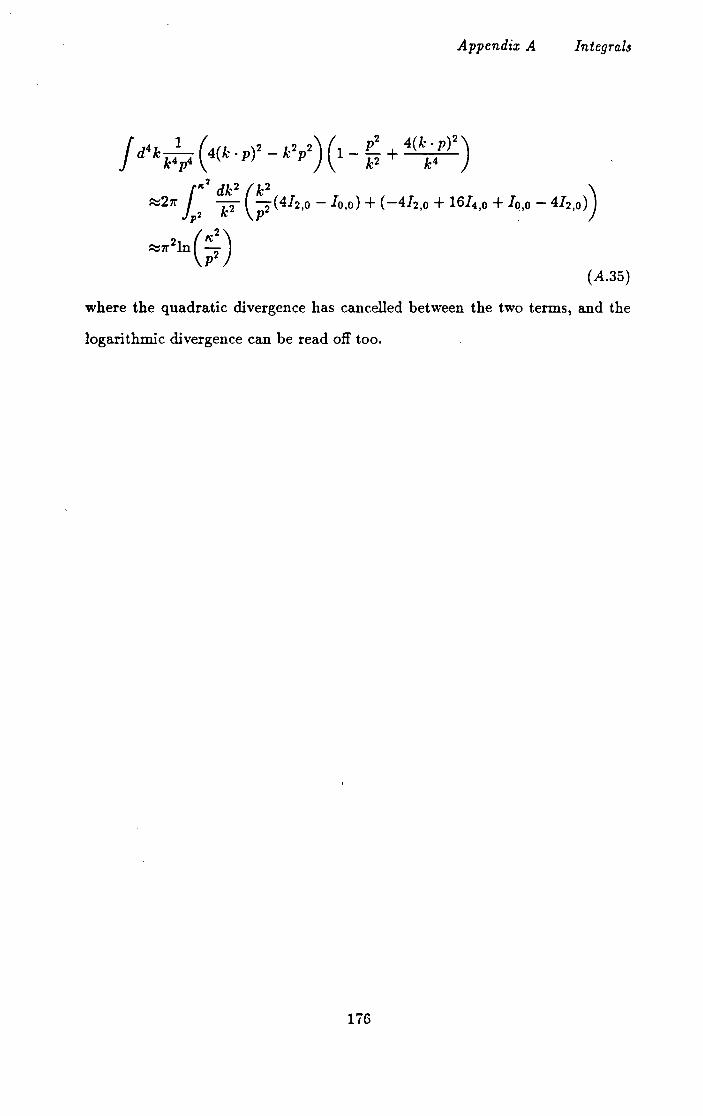
Appendix A Integral3
(A.35)
where the quadratic divergence has cancelled between the two terms, and the
logarithmic divergence can be read off too.
li6

REFERENCES
CHAPTER ONE STRONG INTERACTIONS
[1.1] M. Banner, et al Phys. Lett. 122B (1983) 476
G. Arnison, et al Phys. Lett. 122B (1983) 103
[1.2] E. Rutherford, Phil. Mag. 37 (1919) 581
[1.3] A. Pais, Inward Bound, Oxford university Press, (1986)
[1.4] G. Rochester and C.C. Butler, Nature 160 (1947) 885
[1.5] M. Gell-Mann and Y. Ne'eman, The Eightfold Way, Benjamin New
York, (1964)
S. Okubo, Progr. Theor. Phys. 27 (1962) 949
[1.6] For reviews of QCD see, for example:
W. Marciano and H. Pagels, Phys. Rep. 36 (1978) 137
M.R. Pennington, Rep. Progr. Phys. 46 (1983) 393
[1. 7] For a review of possible confinement mechanisms see:
M. Bander, Phys. Rep. 75 (1981) 207
[1.8] F. Bloch and A. Nordsieclc Phys. Rev. 52 (1937) 54
T. Kinoshita, J. Math. Phys. 3 (1964) 650
T.D. Lee and M. Nauenberg, Phys. Rev. 133 (1964) 1549
For infra-red divergences in QCD see:
J. Frenkel, M-L. Frenkel and J.C. Taylor, Nucl. Phys. B124 (1977) 268
T. Appelquist, J. Carrazone, H. Kluberg-Stern and M. Roth, Phys. Rev.
Lett. 36 (1976) 768
[1.9] J. Cornwall and G. Tiktopoulos Phys. Rev. D13 (1976) 3370
[1.10] K.G. Wilson Phys. Rev. DlO (1974) 2445
For reviews see:
C. Rebbi, Phys. Rep. 67 (1980) 55
J .B. Kogut Phys. Rep. 67 (1980) 67
177
M. ,Creutz Phys. Rep. 95 (1983) 201
CHAPTER TWO THE SCHWINGER-DYSON EQUATIONS
[2.1] For a general account of quantum field theory see:
C. Itzykson and J.B. Zuber, Quantum Field Theory, McGraw-Hill,
(1980); in particular see chapter nine on 'functional methods'.
More details on functional methods are given in:
P. Ramond, Field Theory, a Modern Primer, Benjamin Cummings,
(1981)
C. Nash, Relativistic Quantum Fields, Academic press, (1978)
[2.2] See the first reference of [2.1] as well as:
H. Lehmann, K. Symanzik and \V. Zimmerman, Nuovo Cim. 1 (1955)
205
[2.3] L.D. Fadeev and V.N. Popov, Phys. Lett. 25B (1967) 29
! see also:
T.P. Cheng andL.F. Li, Gauge Theory of Elementary Particle Physics,
Clarendon press, Oxford, (1984)
[2.4] E.J. Eichten and F.L. Feinberg, Phys. Rev. D15 (1977) 2201
[2.5] A.A. Slavnov, Theor. and Math. Phys. 10 (1972) 99
J.C. Taylor, Nucl. Phys. B33 (19il) 436
[2.6] J.C. Ward, Phys. Rev. 78 (1950) 1824
Y. Takahashi, Nuovo Cim. 6 (1957) 370
[2.7] J.S. Ball and T.W. Chui, Phys. Rev. D22 (1980) 2542 and 2550
S.K. Kim and M. Baker, Nucl. Phys. B164 (1980) 152
[2.8] H. Pagels, Phys. Rev. D14 (1976) 2747
H. Pagels, Phys. Rev. D15 (1977) 2991
[2.9] U. Bar-Gadda, Nucl. Phys. B163 (1980) 812
see also ref. [1.6]
178

CHAPTER THREE THE GLUON EQUATION
[3.1] N. Brown and M.R. Pennington Phys. Lett. 106B (1988) 133
[3.2] M. Baker, J.S. Ball and F. Zachariasen, Nucl. Phys. B186 (1981) 531
and 560
[3.3) A.D. Worrall, Ph. D. Thesis submitted to the University of Durham,
unpublished (1985)
M.R. Pennington and A.D. \Vorrall, unpublished, (1983)
CHAPTER FOUR THE MANDELSTAM APPROXIMATION
[4.1] S. Mandelstam, Phys. Rev. D20 (1979) 3223
[4.2] J.S. Ball and F. Zachariasen, Nucl. Phys. B143 (1978) 148
C. Nash and R.L. Stuller, Proc. Roy. Irish Acad. 78 (1978) 217
R. Anishetty, M.Baker, S.K. Kim, J.S. Ball and F. Zachariasen, Phys.
Lett. 86B (1979} 52
M. Baker, J.S. Ball, P. Lucht and F. Zachariasen, Phys. Lett. 89B
(1980) 211
A.I. Alekseev, Yad. Fiz. 33 (1981) 561
W.J. Schoenmaker, Nucl. Phys. B194 (1982) 535
B.A. Arbuzov, Phys. Lett. 125B (1983} 497
E.J. Gardner, J. Phys. G, 9 (1983} 139
D. Atkinson, P.W. Johnson, W.J. Schoenm.aker and B.A. Slim, Nuovo
Cim. A 77 (1983) 197
[4.3] T. Appelquist, M.Dine and I.J. Muzinich, Phys. Lett. 69B (1977) 231
F. Feinberg, Phys. Rev. Lett. 39 (1977) 316
W. Fischler, Nucl. Phys. B129 (1977) 157
[4.4] C. Quigg and J.L. Rosner, Phys. Rep. 56 (1980) 167
[4.5] G.B. West, Phys. Lett. 115B (1982) 468
[4.6] B. Humpert and \V.L. Van Neerven, Phys. Lett. 101B (1981) 101
179
. G. Leibbrandt, Rev. l\1od. Phys. 59 (1987) 1067
[4.7] G.B. 'Vest, Phys. Rev. D27 (1983) 1878
[4.8] M. Creutz, Phys. Rev. DlO (1974) 2696
V.P. Nair and C. Rosenzweig, Phys. Lett. 135B (1984) 450
[4.9] G. 't Hooft, Nucl. Phys. B190 (1981) 455
[4.10] M. Baker, J.S. Ball and F. Zachariasen, Phys. Rev. D37 (1988) 1036
M. Baker, J.S. Ball and F. Zachariasen, Phys. Rev. D31 (1985) 2575
CHAPTER FIVE THE FERMION EQUATION
[5.1] R.L. Stuller, Phys. Rev. D13 (1976) 513
J.S. Ball and F. Zachariasen, Phys. Lett. 106B (1981) 133
H.J. Munczek Phys. Lett. 175B (1986) 215
[5.2] T. Appelquist, M. Bowick, D. Karabali and L.C.R. Wijewardhana,
Phys. Rev. D33 (1986) 3704
D. Atkinson and P.W. Johnson, J. Math. Phys. 28 (1987) 2488
D. Atkinson, P.'\V. Johnson and M. Koopmans, Z. Phys. C34 (1987)
99
D. Atkinson, P.,V. Johnson and K. Stam, Phys. Lett. 201B (1988) 105
[5.3] J.M. Cornwall, Phys. Rev. D22 (1980) 1452
V.S. Gogokhia and B.A. Magradze, Tbilisi report KFKI-1987-01/ A
CHAPTER SIX QUARK LOOPS
[6.1) N. Brown and M.R. Pennington, Brookhaven preprint BNL-41101, to
be published in Phys. Rev. D (1988)
[6.2] M.R. pennington, Phys. Rev. Lett. 60 (1988) 267
CHAPTER SEVEN
QCD
A NON-PERTURBATIVE STUDY OF
[7.1) P. Rambiessa, Phys. Rev. D33 (1986) 2333
180