Akka Decision Engine

An actor based decision engine on the DMN 1.1

specifications

by

Mark Acda, Toon de Boer & Thomas Bos

for the degree of Bachelor of Science at Delft University of Technology

June 25, 2019

Project duration: April 23, 2019 - July 5, 2019Thesis committee: Dr. C.B. Poulsen TU Delft supervisor

Ir. O.W. Visser TU Delft BEP instructorH. Wang TU Delft BEP instructorA. Hagens Finaps product owner

Preface

This report discusses the project we worked on for our Bachelor End Project(BEP) at the TU Delft. We had the privilege to work on a new project atFinaps, an IT company in Amsterdam. This project is to finalise our bachelorand to test our skills that we have learned in the last three years.

When we got the instructions for the BEP, we decided that we wanted todo it at a company to get the feeling of the business life after university andin the hope that what we build will also be used after the project. One of usgot contacted by Finaps via LinkedIn for a job long before the BEP started andthey also said that if he needed to do an internship of any kind he could contactFinaps. That is how we got to Finaps and they were glad to have us to doour BEP for them, because they had a project waiting for us. Finaps alreadywanted to create a decision engine with an actor model before we showed up,but they did not have enough time to start on it, so they gave us this assignmentand it was approved by the TU Delft.

We enjoyed working on this project and seeing good results very quickly keptus motivated. Also the supervisor from Finaps was very glad with the progressand we would like to thank a few people for their help and assistance duringthe project. First of all, we want to thank the very kind people at Finaps forhaving us and especially our product owner Andrew Hagens. Secondly we wantto thank Casper Poulsen, our TU Delft supervisor, for his help, feedback andguidance through this project.

M. Acda, T. de Boer & T. BosDelft, June 2019

1

Summary

Decision engines can decide from a certain input what the output should be.This is done in a table with columns for inputs and outputs and rows for acombination of inputs together with its corresponding output. A row is alsocalled a rule. A simple program to decide such a decision table can easily bemade, like Camunda. However, when the output of one table is also the inputof another table and so on and the amount of rules get enormously big, theproblem gets more complicated and Camunda takes a very long time to solvesuch structures.

We created a decision engine in Scala that can decide the output when thereare thousands of tables linked together in less than a minute with the help ofAkka. Akka is an actor model, which means that it can create multiple actors,which each can perform a certain task. Actors can run in parallel, which speedsup the decision engine. Actors send messages to each other and an actor willonly start working when they receive a message. The decision engine readsDMN files and parses it to tables. For better performance the decision tablesget parsed into a tree structure with for every table the input tables are itschildren. In this way the decision engine is very quick in solving tables, howeverthe parsing into trees still takes some time. This is not a big problem, since theparsing is only done once and the tree can be saved and the solving can be donevery often. Also the deciding of a single table is improved, because we createdour own FEEL-expressions that can decide the rules very fast.

The result is that after a very large table with 50,000 rules is parsed, thesolving that took Camunda 400 milliseconds only takes 9 milliseconds for thenew decision engine and when the parsing is left out, the new engine is faster incomputing 500,000 rules than Camunda with 1 rule. Also when the parsing isincluded in the time, the difference gets only bigger. For 50,000 rules, Camundatakes 20 seconds to parse the file and solve the table, while the new decisionengine takes only a little more than 1 second to do this all. When the files getlarger, so does the difference.

2

Contents

1 Introduction 5

2 Background 92.1 Decision Model and Notation . . . . . . . . . . . . . . . . . . . . 9

2.1.1 How DMN works . . . . . . . . . . . . . . . . . . . . . . . 102.1.2 DMN 1.1 or DMN 1.2 . . . . . . . . . . . . . . . . . . . . 10

2.2 Camunda . . . . . . . . . . . . . . . . . . . . . . . . . . . . . . . 112.3 Akka . . . . . . . . . . . . . . . . . . . . . . . . . . . . . . . . . . 11

2.3.1 Actor Model . . . . . . . . . . . . . . . . . . . . . . . . . 132.3.2 Why Akka . . . . . . . . . . . . . . . . . . . . . . . . . . 142.3.3 Scala vs Java . . . . . . . . . . . . . . . . . . . . . . . . . 14

3 Problem definition and analysis 163.1 Requirements as stated by the client . . . . . . . . . . . . . . . . 163.2 Scope . . . . . . . . . . . . . . . . . . . . . . . . . . . . . . . . . 16

4 Design and implementation 174.1 DRD . . . . . . . . . . . . . . . . . . . . . . . . . . . . . . . . . . 174.2 Decision Tree . . . . . . . . . . . . . . . . . . . . . . . . . . . . . 174.3 Actors . . . . . . . . . . . . . . . . . . . . . . . . . . . . . . . . . 19

4.3.1 Structure and tasks . . . . . . . . . . . . . . . . . . . . . 194.3.2 Messaging . . . . . . . . . . . . . . . . . . . . . . . . . . . 19

4.4 API . . . . . . . . . . . . . . . . . . . . . . . . . . . . . . . . . . 204.4.1 Input . . . . . . . . . . . . . . . . . . . . . . . . . . . . . 204.4.2 Output . . . . . . . . . . . . . . . . . . . . . . . . . . . . 21

4.5 Sequence diagram . . . . . . . . . . . . . . . . . . . . . . . . . . . 22

5 Evaluation 235.1 Performance . . . . . . . . . . . . . . . . . . . . . . . . . . . . . . 23

5.1.1 Performance monitoring . . . . . . . . . . . . . . . . . . . 235.1.2 Benchmarking against Camunda on varying number of rules 255.1.3 Benchmarking against Camunda on varying number of

tables . . . . . . . . . . . . . . . . . . . . . . . . . . . . . 275.1.4 Speed comparison for different settings of actor model . . 30

3

5.2 Behaviour . . . . . . . . . . . . . . . . . . . . . . . . . . . . . . . 315.2.1 Test environment . . . . . . . . . . . . . . . . . . . . . . . 31

5.3 Code quality . . . . . . . . . . . . . . . . . . . . . . . . . . . . . 325.4 Development Process . . . . . . . . . . . . . . . . . . . . . . . . . 33

5.4.1 Scrum . . . . . . . . . . . . . . . . . . . . . . . . . . . . . 335.4.2 Git . . . . . . . . . . . . . . . . . . . . . . . . . . . . . . . 345.4.3 Continuous Integration . . . . . . . . . . . . . . . . . . . 345.4.4 Problems encountered during development . . . . . . . . . 34

6 Discussion and recommendations 366.1 Results . . . . . . . . . . . . . . . . . . . . . . . . . . . . . . . . . 36

6.1.1 Quality of the comparison . . . . . . . . . . . . . . . . . . 366.2 Bottleneck . . . . . . . . . . . . . . . . . . . . . . . . . . . . . . . 376.3 Overhead of Akka . . . . . . . . . . . . . . . . . . . . . . . . . . 376.4 Future work . . . . . . . . . . . . . . . . . . . . . . . . . . . . . . 376.5 Ethical issues . . . . . . . . . . . . . . . . . . . . . . . . . . . . . 38

7 Conclusions 39

Appendices 42

A Weekly activities 43A.1 Week 1 - Research . . . . . . . . . . . . . . . . . . . . . . . . . . 43A.2 Week 2 - Research . . . . . . . . . . . . . . . . . . . . . . . . . . 43A.3 Week 3 - Development . . . . . . . . . . . . . . . . . . . . . . . . 43A.4 Week 4 - Development . . . . . . . . . . . . . . . . . . . . . . . . 43A.5 Week 5 - Development . . . . . . . . . . . . . . . . . . . . . . . . 44A.6 Week 6 - Development . . . . . . . . . . . . . . . . . . . . . . . . 44A.7 Week 7 - Development . . . . . . . . . . . . . . . . . . . . . . . . 44A.8 Week 8 - Development . . . . . . . . . . . . . . . . . . . . . . . . 44A.9 Week 9 - Development . . . . . . . . . . . . . . . . . . . . . . . . 44A.10 Week 10 - Development . . . . . . . . . . . . . . . . . . . . . . . 44A.11 Week 11 - Presentation . . . . . . . . . . . . . . . . . . . . . . . . 44

B MoSCoW 45B.1 Must haves . . . . . . . . . . . . . . . . . . . . . . . . . . . . . . 45B.2 Should haves . . . . . . . . . . . . . . . . . . . . . . . . . . . . . 45B.3 Could haves . . . . . . . . . . . . . . . . . . . . . . . . . . . . . . 46B.4 Won’t haves . . . . . . . . . . . . . . . . . . . . . . . . . . . . . . 46

C Speed comparison data 47C.1 Benchmark between Camunda’s program and our program . . . . 47C.2 Comparison between multiple parameters about number of actors 49

C.2.1 One input . . . . . . . . . . . . . . . . . . . . . . . . . . . 49C.2.2 30 inputs at the same time . . . . . . . . . . . . . . . . . 50

4

Chapter 1

Introduction

In current businesses, there are a lot of problems that needs to be decided. Thedecision-making is automated to increase the efficiency. But bigger companiesneed to take more and more decisions. To keep up with the increasing amount ofdecisions they also need to be made faster. The problem of the existing softwarefor decision-making is that they are not scalable. When the load becomes toohigh, they are not able to decide efficiently anymore. Therefore, the questionthat this project tries to answer is: Is it possible to create a well tested decisionengine for the DMN specification, using the Akka actor system, that performsvery well on a very high load?

The background for this project and all the libraries and tools which are usedduring the project will be discussed in chapter 2. The problems to be solvedby this project are stated and analysed in chapter 3 and chapter 4 discussesthe design choices and implementation of the decision engine. The results anddevelopment process will be evaluated in chapter 5. The discussion and futurework recommendations can be found in chapter 6. In the final chapter, chapter7, the conclusion can be found.

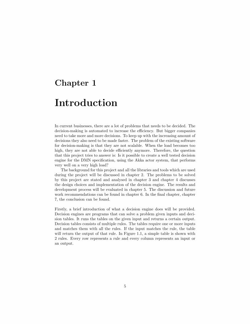
Firstly, a brief introduction of what a decision engine does will be provided.Decision engines are programs that can solve a problem given inputs and deci-sion tables. It runs the tables on the given input and returns a certain output.Decision tables consists of multiple rules. The tables require one or more inputsand matches them with all the rules. If the input matches the rule, the tablewill return the output of that rule. In Figure 1.1, a simple table is shown with2 rules. Every row represents a rule and every column represents an input oran output.

5

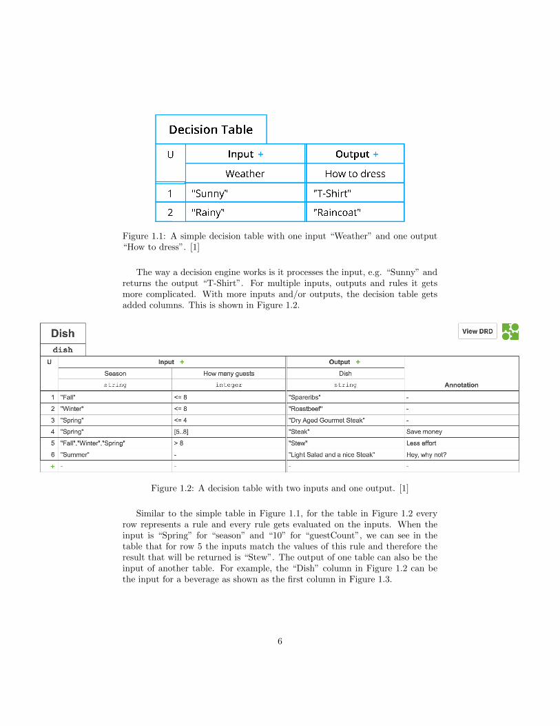
Figure 1.1: A simple decision table with one input “Weather” and one output“How to dress”. [1]

The way a decision engine works is it processes the input, e.g. “Sunny” andreturns the output “T-Shirt”. For multiple inputs, outputs and rules it getsmore complicated. With more inputs and/or outputs, the decision table getsadded columns. This is shown in Figure 1.2.

Figure 1.2: A decision table with two inputs and one output. [1]

Similar to the simple table in Figure 1.1, for the table in Figure 1.2 everyrow represents a rule and every rule gets evaluated on the inputs. When theinput is “Spring” for “season” and “10” for “guestCount”, we can see in thetable that for row 5 the inputs match the values of this rule and therefore theresult that will be returned is “Stew”. The output of one table can also be theinput of another table. For example, the “Dish” column in Figure 1.2 can bethe input for a beverage as shown as the first column in Figure 1.3.

6

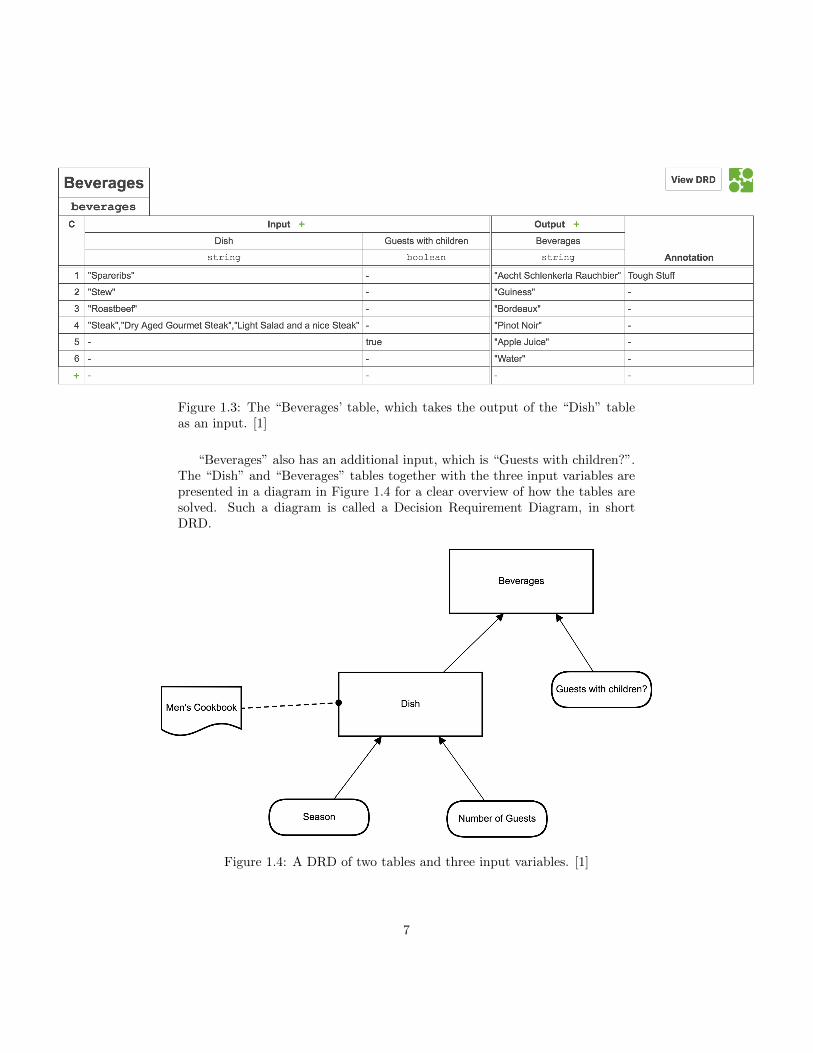
Figure 1.3: The “Beverages’ table, which takes the output of the “Dish” tableas an input. [1]

“Beverages” also has an additional input, which is “Guests with children?”.The “Dish” and “Beverages” tables together with the three input variables arepresented in a diagram in Figure 1.4 for a clear overview of how the tables aresolved. Such a diagram is called a Decision Requirement Diagram, in shortDRD.

Figure 1.4: A DRD of two tables and three input variables. [1]

7

A decision engine will solve the DRD in 1.4 by first solving the Dish tablewith the inputs of “Season” and “Number of Guests”. After that it will takethe dish output and solve the “Beverages” table with this output and the inputof “Guests with children?”. This table will return the beverages correspondingto the rules for which the inputs match.

8

Chapter 2

Background

Before going more in depth about the problems and features of this project, somebackground information is provided in this chapter. Different technologies willbe discussed that were used to develop the final product. First of all the DecisionModel and Notation is explained and why it is important for our project. Afterthat the platforms Camunda and Akka will be discussed in more detail. Finallythe reason why this project is coded in Scala instead of Java will be explained.

2.1 Decision Model and Notation

Decision Model and Notation (DMN) provides a construct to model decisions,so that they can be understood by business analysts, technical developers, etc.[2]. DMN bridges the gap between business decision design and decision imple-mentation.

9

Figure 2.1: An example of a Decision Requirements Diagram (DRD). [3]

2.1.1 How DMN works

DMN provides a specification to create so called Decision Requirement Diagrams(DRD). These diagrams consist of the following elements [4]:

• Input data: represents an input. (e.g. “Person” in Figure 2.1)

• Decisions: gives output from a number of inputs. The output is deter-mined by a set of rules depicted in a table. (e.g. “Address Verified” inFigure 2.1)

• Business Knowledge Model (BKM): functions providing logic for multipledecision elements.

• Knowledge Source: describes the way decisions are made and how it usesthe input data. (e.g. “AML Regulations” in Figure 2.1)

Each decision is composed of a set of rules depicted in a table. An exampleof a decision table can be seen in Figure 2.2.

2.1.2 DMN 1.1 or DMN 1.2

The latest version of DMN is version 1.2 which came out in January 2019 [2].Version 1.2 improves over version 1.1 in that it generally adds more flexibility inthe creation of DRDs, but does not add any big features that set both versionsapart [5]. Because of the existence of a DMN parser for DMN version 1.1 and

10

Figure 2.2: An example decision table [3]. This table has three inputs, oneoutput and six rules. If, for instance, the inputs are “Private” for “ClientType”, $30000 for “On Deposit” and “Medium” for “Estimated Net Worth”,then the output of this decision will be “Personal Wealth Management”.

not for 1.2 (which will be discussed in section 2.2), we opted to use DMN version1.1.

2.2 Camunda

Camunda is an open source platform for workflow and decision automation thatbrings business users and software developers together [1]. With Camunda youcan make your own DRDs, parse and execute them, but we only used Camundato create DRDs for testing and benchmarking. Camunda has written their codebase in Java and builds on the older spec version DMN 1.1. It is important tonote that the Camunda DMN parser ignores Knowledge Sources and BKMs asthey are optional.

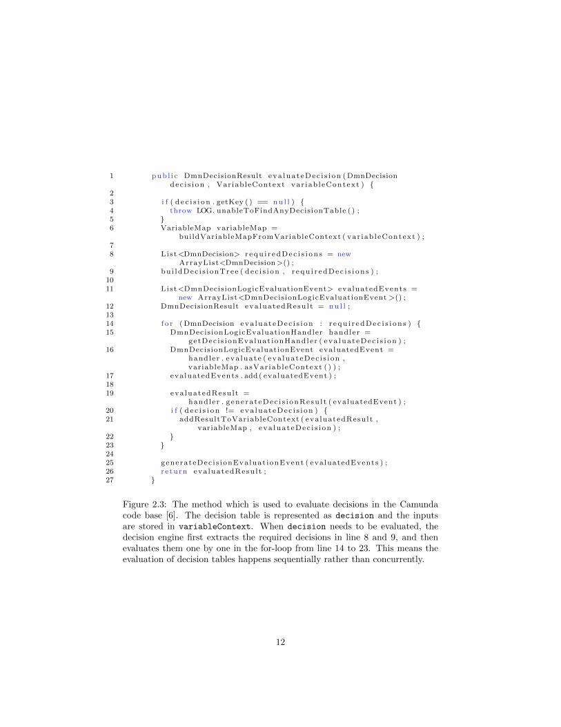
The main problem with Camunda is that Camunda is very slow in solvingDRDs and especially in solving multiple DRDs at the same time with differ-ent inputs. From inspection of the base code [6], mostly by debugging actualevaluation runs, it was deduced that no concurrency is used in the calculatingof results. This can be seen in the code snippet in Figure 2.3. Therefore, thisproject aims to create a system based on the actor model to provide concurrencyand therefore higher throughput than the Camunda counterpart.

2.3 Akka

The Akka library is a toolkit for building highly concurrent, distributed, and re-silient message-driven applications for Java and Scala and is an implementationof the actor model on the Java Virutal Machine (JVM) [7].

11

1 pub l i c DmnDecisionResult eva lua t eDec i s i on (DmnDecisiondec i s i on , Var iableContext var iab l eContext ) {

23 i f ( d e c i s i o n . getKey ( ) == nu l l ) {4 throw LOG. unableToFindAnyDecisionTable ( ) ;5 }6 VariableMap variableMap =

buildVariableMapFromVariableContext ( var iab leContext ) ;78 List<DmnDecision> r e qu i r edDec i s i on s = new

ArrayList<DmnDecision>() ;9 bu i ldDec i s i onTree ( dec i s i on , r e qu i r edDec i s i on s ) ;

1011 List<DmnDecisionLogicEvaluationEvent> evaluatedEvents =

new ArrayList<DmnDecisionLogicEvaluationEvent >() ;12 DmnDecisionResult eva luatedResu l t = nu l l ;1314 f o r (DmnDecision eva lua t eDec i s i on : r e qu i r edDec i s i on s ) {15 DmnDecisionLogicEvaluationHandler handler =

getDec i s ionEva luat ionHandle r ( eva lua t eDec i s i on ) ;16 DmnDecisionLogicEvaluationEvent evaluatedEvent =

handler . eva luate ( eva luateDec i s i on ,variableMap . asVar iableContext ( ) ) ;

17 evaluatedEvents . add ( evaluatedEvent ) ;1819 eva luatedResu l t =

handler . g ene ra t eDec i s i onResu l t ( evaluatedEvent ) ;20 i f ( d e c i s i o n != eva lua t eDec i s i on ) {21 addResultToVariableContext ( eva luatedResu l t ,

variableMap , eva lua t eDec i s i on ) ;22 }23 }2425 generateDec i s ionEva luat ionEvent ( evaluatedEvents ) ;26 re turn eva luatedResu l t ;27 }

Figure 2.3: The method which is used to evaluate decisions in the Camundacode base [6]. The decision table is represented as decision and the inputsare stored in variableContext. When decision needs to be evaluated, thedecision engine first extracts the required decisions in line 8 and 9, and thenevaluates them one by one in the for-loop from line 14 to 23. This means theevaluation of decision tables happens sequentially rather than concurrently.

12

2.3.1 Actor Model

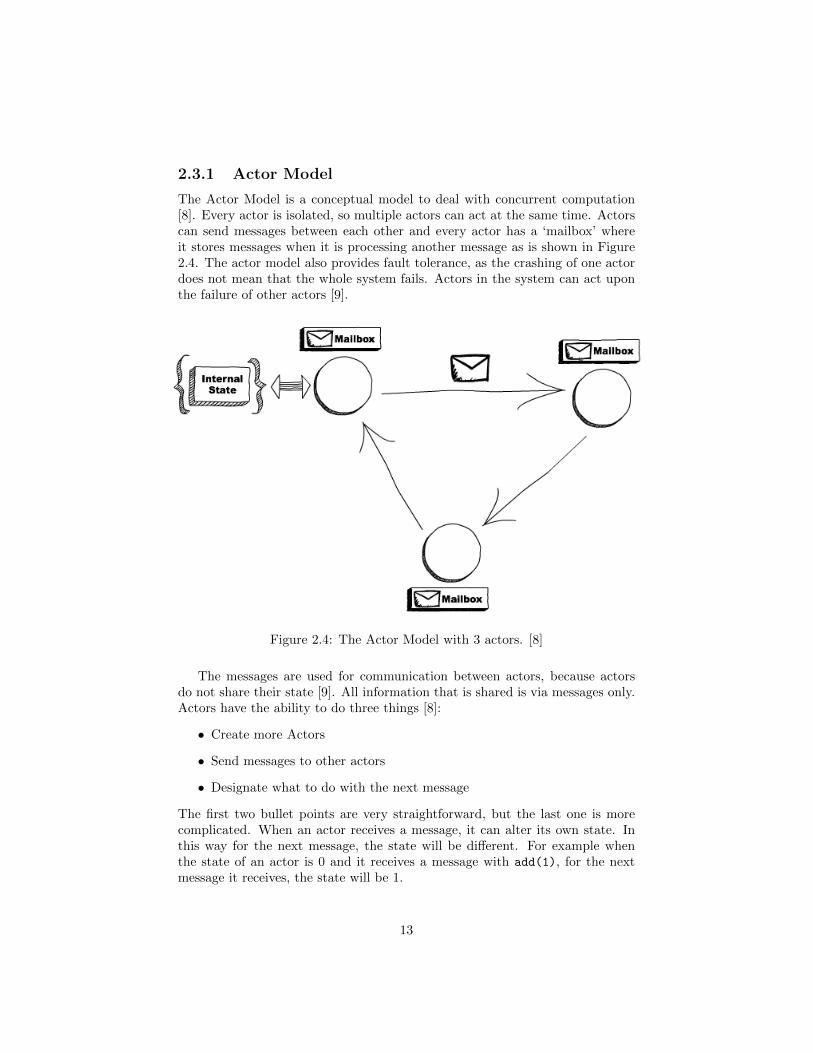
The Actor Model is a conceptual model to deal with concurrent computation[8]. Every actor is isolated, so multiple actors can act at the same time. Actorscan send messages between each other and every actor has a ‘mailbox’ whereit stores messages when it is processing another message as is shown in Figure2.4. The actor model also provides fault tolerance, as the crashing of one actordoes not mean that the whole system fails. Actors in the system can act uponthe failure of other actors [9].

Figure 2.4: The Actor Model with 3 actors. [8]

The messages are used for communication between actors, because actorsdo not share their state [9]. All information that is shared is via messages only.Actors have the ability to do three things [8]:

• Create more Actors

• Send messages to other actors

• Designate what to do with the next message

The first two bullet points are very straightforward, but the last one is morecomplicated. When an actor receives a message, it can alter its own state. Inthis way for the next message, the state will be different. For example whenthe state of an actor is 0 and it receives a message with add(1), for the nextmessage it receives, the state will be 1.

13

2.3.2 Why Akka

We choose Akka as our actor framework, because it has high performance andit lets us build a system that can scale by using multiple servers. Akka is ableto distribute tasks in different threads and run those in parallel, therefore theefficiency increases and there is a significant speed-up. The creation of the actorsand sending and retrieving of messages comes with an overhead. However, Akkahas been proven to be significantly faster than 4 other actor models [10] andhas the least overhead of all, because it runs directly on the JVM.

Messages

Messages are used to send data between actors asynchronously, where the datacan be of any type, but it must be immutable [7]. Akka has two types ofmessages, Ask and Tell messages. A Tell message sends the data, and that’s it.The Ask message also creates a return object which encapsulates the possiblereply. When it is ready, the reply can be extracted from it. Separate actionscan be specified for when the reply was succeeded (the return object is given)or failed (an exception is thrown). This makes the Ask message easier to workwith, but also creates some overhead. The messages between actors makes Akkaa perfect tool for our decision engine. How these messages are implemented willbe explained in Section 4.3.2.

Actor Hierarchy

Another advantage of Akka is that it has a built in fault tolerance model whichallows applications to fail and recover as soon as possible [9]. All actors arestructured in an actor hierarchy which looks like a tree. Every actors parentalso acts as a supervisor actor, which gets notified if an actor crashes [8]. Thesupervisor can do something about it to return the actor to a consistent stateagain (e.g. returning it to its initial state).

2.3.3 Scala vs Java

We had the option to write our program in Scala or in Java, because Akka has anAPI for only those two languages. Our choice is to use Scala, because we believethat Scala has some nice benefits over Java. An empirical study has shown thatScala code is more compact [11]. Moreover, developers say that Scala is so muchmore than Java thanks to its expressive type-system [12] and Scala is both anobject-oriented and functional programming language. The performance is alsoan important aspect when choosing the programming language, but the APIperformance of Akka should not differ for both languages. Therefore neitherone is much better for the API. But besides the API, Scala should run about20% faster than Java according to a benchmark on sorting 100.000 items 100times by writing similar code for both languages [13].

A huge benefit for this project in particular are Monads, which are objectsthat wrap values of any type. For example the Option object that allows a

14

value to be Some(value), where value can be of any type, or None is used alot. In particular the Scala Future compared to a Thread in Java is a greatadvantage of Scala [14]. Both are used to run code in parallel. A Thread doesnot have a return type while a Future is an object that holds a value that doesnot yet exists but which may become available at some point. This is used alot with sending return messages to the parent actor from child actors, thatrun concurrently. The actor structure and messaging of this project is furtherexplained in section 4.3.

15

Chapter 3

Problem definition andanalysis

This chapter discusses the requirements as stated by the client and the scope inwhich this project needs to be created.

3.1 Requirements as stated by the client

The requirements for this project are to create a decision engine that performsvery well on a very high load with multiple inputs at the same time. It hasto be an improvement over the existing decision engine software by Camunda[1] by being faster and concurrent. Furthermore, it should use the Akka actormodel to provide that needed concurrency. The decision engine should be ableto use at least the DMN 1.1 spec .dmn files and it should be able to be callableby API. It should then accept input in the format:

{dmnId:[dmnId],[param1]:[val1],[param2]:[val2],...}

The API should then return the computed result and a representation of thedecisions made to arrive at said result.

3.2 Scope

The Decision Engine is supposed to run continuously and it must be callableby API. A big requirement for the solution is to be simple but effective andthe focus is not laid on the front-end but rather on the back-end where thecomputations are done, and these computations need to be done with veryhigh throughput. This means that the decision engine will not feature a userinterface. It should, however, be able to output a representation of the way theoutput was generated in the decision engine. A MoSCoW representation of therequirements and scope can be seen in Appendix B.

16

Chapter 4

Design and implementation

In order to arrive at an implementation which satisfied the requirements, anumber of design decisions had to be made. In this chapter, the workings ofeach component and the reasoning behind the design are given.

4.1 DRD

The DRDs used as input to the system are stored in .dmn files. These filesare used by Camunda and represent DRDs in XML form and can be generatedusing the Camunda Modeler [15]. Due to the XML structure they can easily beinterpreted and converted into decision trees.

4.2 Decision Tree

In order to solve a DRD using actors, the choice was made to first convertit into a decision tree. The tree is constructed by taking the output decisiontables as nodes and appending their inputs as child nodes and then continuouslyadd inputs to decision tables until an input element is reached. The result ofconverting the DRD in Figure 4.1 to a decision tree is shown in Figure 4.2.The advantage of using decision trees is that each tree branch can be solvedconcurrently without requirements from parallel branches. As you can see inFigure 4.2, some tables occur multiple times in the tree, because they are aninput of different tables. This will not take more memory, because the sametables point to the same memory address, which will also make the solving ofthe tables faster. When the table has been solved once, the output is saved andwill be used at all other places in the tree.

17

Figure 4.1: An example DRD.

Figure 4.2: The decision tree from the DRD from Figure 4.1

18

4.3 Actors

In order to achieve concurrency the Akka actor system is used. In this frameworkactors are structured in a hierarchy and communicate by sending messages toeach other. An actor performs an action as a reaction to each message it receives.

4.3.1 Structure and tasks

In this project the actor hierarchy consists of two branches: the parsing branchand the solving branch. This can be viewed in Figure 4.3. The parsing branchhandles the parsing of the DRDs into decision trees and the solving branchhandles the evaluating of decision trees on input. The ParserSupervisor andthe SolverSupervisor actors handle communication with the Master actorand monitor their children, the Parser and TreeSolver actors. Parser actorsparse DRDs into decision trees with the help of the OutputNodeFinder andInputNodeFinder actors. TreeSolver actors evaluate decision trees on inputand makes use of ElementSolver actors which evaluate individual decision treeelements on the given input values.

Figure 4.3: The actor hierarchy.

4.3.2 Messaging

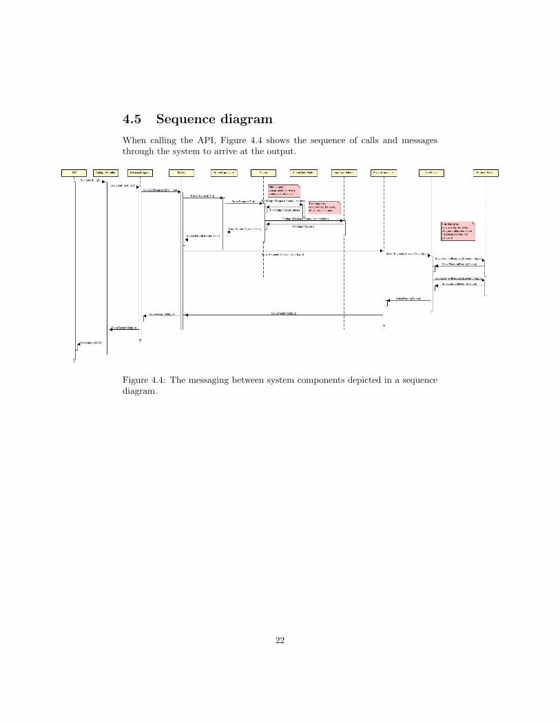
The Master actor receives SolveDrdRequest(drd, input, save, refresh)

messages from the decision engine, asking it to solve a given DRD on an in-

19

put. The Master then checks whether the given DRD has already been parsedinto a decision tree. If not, or if the Master is asked to refresh the decision tree,it will send a ParseRequest(drd, save) message to the ParserSupervisor

actors requesting it to convert a DRD into a decision tree. The ParserSu-

pervisor actor will then allocate one of its child actors, the Parser actors, toconvert the DRD. The Parser actor will first split the list of all tables in multi-ple chunks and sends for each chunk a FindOutputRequest(chunk, inputIds)

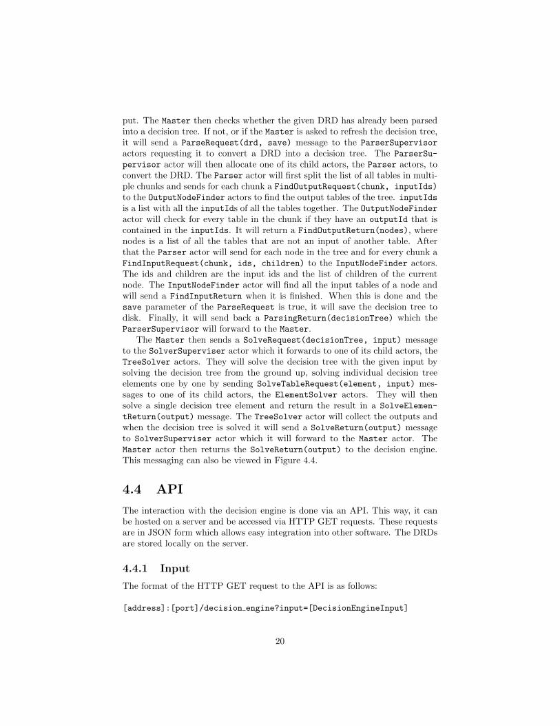
to the OutputNodeFinder actors to find the output tables of the tree. inputIdsis a list with all the inputIds of all the tables together. The OutputNodeFinderactor will check for every table in the chunk if they have an outputId that iscontained in the inputIds. It will return a FindOutputReturn(nodes), wherenodes is a list of all the tables that are not an input of another table. Afterthat the Parser actor will send for each node in the tree and for every chunk aFindInputRequest(chunk, ids, children) to the InputNodeFinder actors.The ids and children are the input ids and the list of children of the currentnode. The InputNodeFinder actor will find all the input tables of a node andwill send a FindInputReturn when it is finished. When this is done and thesave parameter of the ParseRequest is true, it will save the decision tree todisk. Finally, it will send back a ParsingReturn(decisionTree) which theParserSupervisor will forward to the Master.

The Master then sends a SolveRequest(decisionTree, input) messageto the SolverSuperviser actor which it forwards to one of its child actors, theTreeSolver actors. They will solve the decision tree with the given input bysolving the decision tree from the ground up, solving individual decision treeelements one by one by sending SolveTableRequest(element, input) mes-sages to one of its child actors, the ElementSolver actors. They will thensolve a single decision tree element and return the result in a SolveElemen-

tReturn(output) message. The TreeSolver actor will collect the outputs andwhen the decision tree is solved it will send a SolveReturn(output) messageto SolverSuperviser actor which it will forward to the Master actor. TheMaster actor then returns the SolveReturn(output) to the decision engine.This messaging can also be viewed in Figure 4.4.

4.4 API

The interaction with the decision engine is done via an API. This way, it canbe hosted on a server and be accessed via HTTP GET requests. These requestsare in JSON form which allows easy integration into other software. The DRDsare stored locally on the server.

4.4.1 Input

The format of the HTTP GET request to the API is as follows:

[address]:[port]/decision engine?input=[DecisionEngineInput]

20

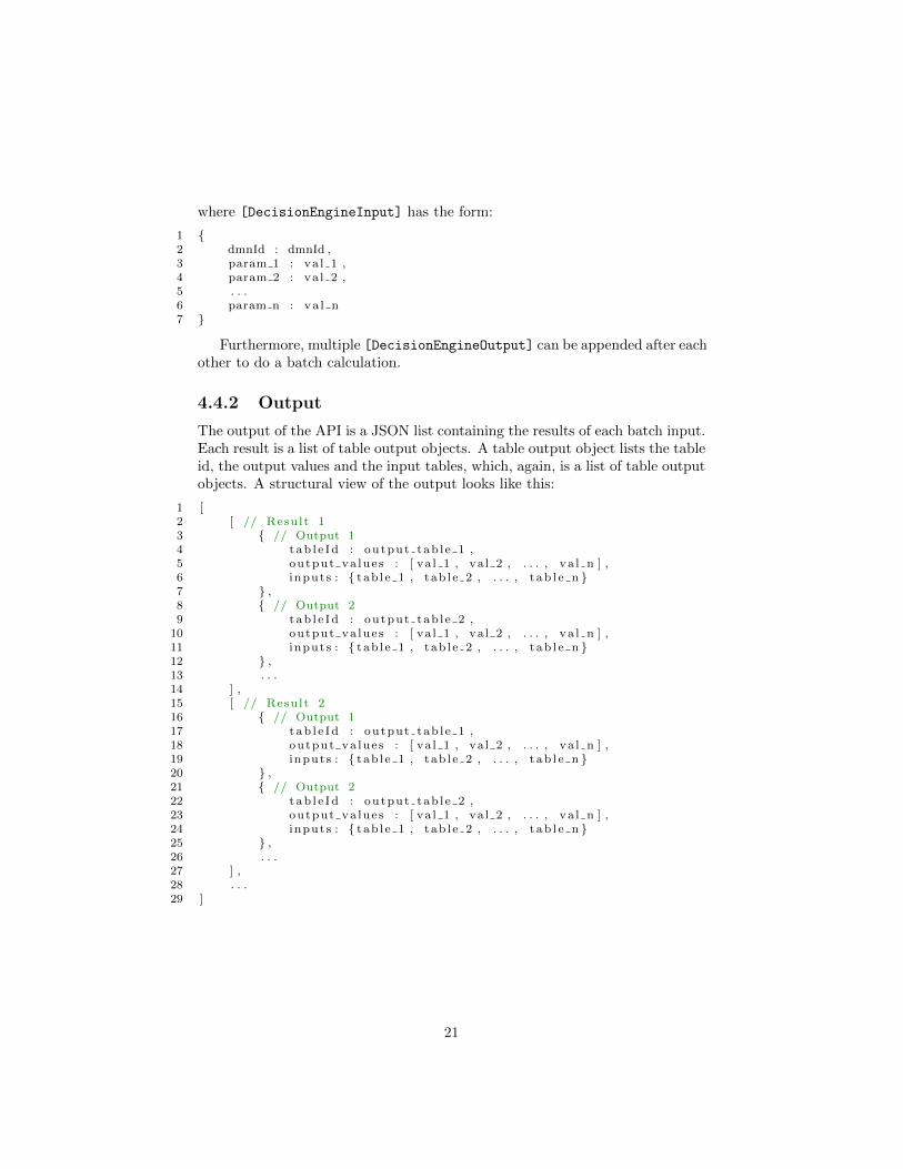
where [DecisionEngineInput] has the form:

1 {2 dmnId : dmnId ,3 param 1 : va l 1 ,4 param 2 : va l 2 ,5 . . .6 param n : va l n7 }

Furthermore, multiple [DecisionEngineOutput] can be appended after eachother to do a batch calculation.

4.4.2 Output

The output of the API is a JSON list containing the results of each batch input.Each result is a list of table output objects. A table output object lists the tableid, the output values and the input tables, which, again, is a list of table outputobjects. A structural view of the output looks like this:

1 [2 [ // Result 13 { // Output 14 tab l e Id : output tab l e 1 ,5 output va lue s : [ va l 1 , va l 2 , . . . , va l n ] ,6 inputs : { tab l e 1 , tab l e 2 , . . . , t ab l e n }7 } ,8 { // Output 29 tab l e Id : output tab l e 2 ,

10 output va lue s : [ va l 1 , va l 2 , . . . , va l n ] ,11 inputs : { tab l e 1 , tab l e 2 , . . . , t ab l e n }12 } ,13 . . .14 ] ,15 [ // Result 216 { // Output 117 tab l e Id : output tab l e 1 ,18 output va lue s : [ va l 1 , va l 2 , . . . , va l n ] ,19 inputs : { tab l e 1 , tab l e 2 , . . . , t ab l e n }20 } ,21 { // Output 222 tab l e Id : output tab l e 2 ,23 output va lue s : [ va l 1 , va l 2 , . . . , va l n ] ,24 inputs : { tab l e 1 , tab l e 2 , . . . , t ab l e n }25 } ,26 . . .27 ] ,28 . . .29 ]

21

4.5 Sequence diagram

When calling the API, Figure 4.4 shows the sequence of calls and messagesthrough the system to arrive at the output.

Figure 4.4: The messaging between system components depicted in a sequencediagram.

22

Chapter 5

Evaluation

After the design and implementation, the performance and the behaviour of thesystem need to be evaluated in order to check whether it satisfies the require-ments. It is also important to evaluate the development process and methods.The evaluation methods and results will be discussed in this chapter.

5.1 Performance

In order to test the performance of individual system components, or benchmarkthe system against its Camunda counterpart, a number of methods were used.

5.1.1 Performance monitoring

In order to view the raw performance of the system, a number of methods wereused in different stages of development to find out whether the system wasproviding desirable performance.

Stopwatch

The most basic solution was to use the ‘stopwatch’ method; basically mea-suring the time it takes to do a calculation. This method’s reliability is notensured though, as run times are dependent on outside factors like processorload, amount of free memory, and JVM garbage collection can occur in thebackground, at any given time, which also uses processing power which thencannot be used by the decision engine [16], resulting in inconsistent times.

JProfiler

A more reliable and trustworthy method is to use JProfiler [17]. This softwaremonitors the project when it runs and accurately measures the amount of timethe JVM stays in each bit of code. This way, when the process is done, thebottlenecks of the system become clear which makes system analysis a lot easier.

23

The bottlenecks can be methods which have lots of self-time or big amounts ofobjects which clog memory because they are stored in the background. JProfilerwas used extensively in the later stages of the project when the code base wasfully functional, but needed optimisation.

Below are two snapshots of the CPU usage during solving. The second snap-shot was taken 3.5 weeks after the first one. Let’s take the second line of Figure5.1 to explain what the numbers are. This line shows that the JVM is for 67.5%of the total run time in the method actor.ElementSolver.aroundReceive.The total duration of the method is 303 seconds. 612 milliseconds are in themethod itself (called self-time), the other part of the time is in the methods itcalls. The method is called 1, 738, 787 times.

Figure 5.1 shows a snapshot where we started using JProfiler. What stoodout was how much time operations on lists took. For example, the program isfor 11.0% of the time in the method List.distinct.

Figure 5.1: JProfiler snapshot 23rd of May.

After more than three weeks of optimising, methods with a large amount ofself-time are optimised. The result is visible in Figure 5.2. As you can see, thenumber of calls to a method in List is drastically reduced. The total run time ofthe method dmn.DecisionTableElement.calculateOutput dropped from 265

24

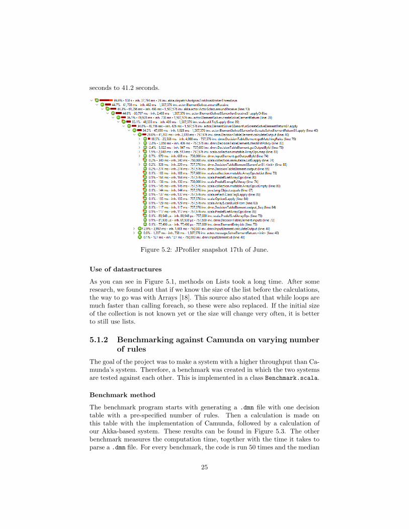
seconds to 41.2 seconds.

Figure 5.2: JProfiler snapshot 17th of June.

Use of datastructures

As you can see in Figure 5.1, methods on Lists took a long time. After someresearch, we found out that if we know the size of the list before the calculations,the way to go was with Arrays [18]. This source also stated that while loops aremuch faster than calling foreach, so these were also replaced. If the initial sizeof the collection is not known yet or the size will change very often, it is betterto still use lists.

5.1.2 Benchmarking against Camunda on varying numberof rules

The goal of the project was to make a system with a higher throughput than Ca-munda’s system. Therefore, a benchmark was created in which the two systemsare tested against each other. This is implemented in a class Benchmark.scala.

Benchmark method

The benchmark program starts with generating a .dmn file with one decisiontable with a pre-specified number of rules. Then a calculation is made onthis table with the implementation of Camunda, followed by a calculation ofour Akka-based system. These results can be found in Figure 5.3. The otherbenchmark measures the computation time, together with the time it takes toparse a .dmn file. For every benchmark, the code is run 50 times and the median

25

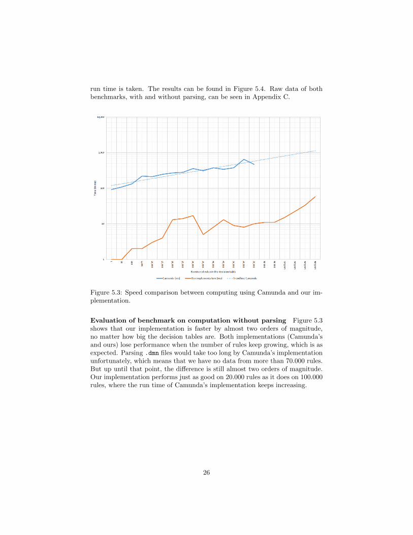
run time is taken. The results can be found in Figure 5.4. Raw data of bothbenchmarks, with and without parsing, can be seen in Appendix C.

Figure 5.3: Speed comparison between computing using Camunda and our im-plementation.

Evaluation of benchmark on computation without parsing Figure 5.3shows that our implementation is faster by almost two orders of magnitude,no matter how big the decision tables are. Both implementations (Camunda’sand ours) lose performance when the number of rules keep growing, which is asexpected. Parsing .dmn files would take too long by Camunda’s implementationunfortunately, which means that we have no data from more than 70.000 rules.But up until that point, the difference is still almost two orders of magnitude.Our implementation performs just as good on 20.000 rules as it does on 100.000rules, where the run time of Camunda’s implementation keeps increasing.

26

Figure 5.4: Speed comparison between computing and parsing using Camundaand our implementation.

Evaluation of benchmark on computation with parsing The improve-ments are even greater during parsing of the .dmn files, as you can see in Figure5.4. With a small amount of rules, both implementations differ for about oneorder of magnitude from each other in favour of our implementation. Whenthe amount of rules keeps growing, the difference in speed also keeps growing.In the end, we stopped measuring the parsing of the Camunda code becauseit just took too long. Extrapolating the data shows that with 500.000 rules,Camunda’s parsing would take over five hours (see dotted line in Figure 5.4).This is a difference of already three orders of magnitude.

5.1.3 Benchmarking against Camunda on varying numberof tables

We are using the same benchmark as above, but now with a varying number ofdecision tables instead of rules. The benchmark program starts with generatingmultiple DRDs which are saved to .dmn files, all with different configurations. Itcontains decision trees linked to each other in a tree-like structure. The variablesare number of children, and number of layers. The leave tables are the inputtables, and the root table is the tables which gives the output. To clarify this,let’s give an example. Three layers and four children means that the root table’s

27

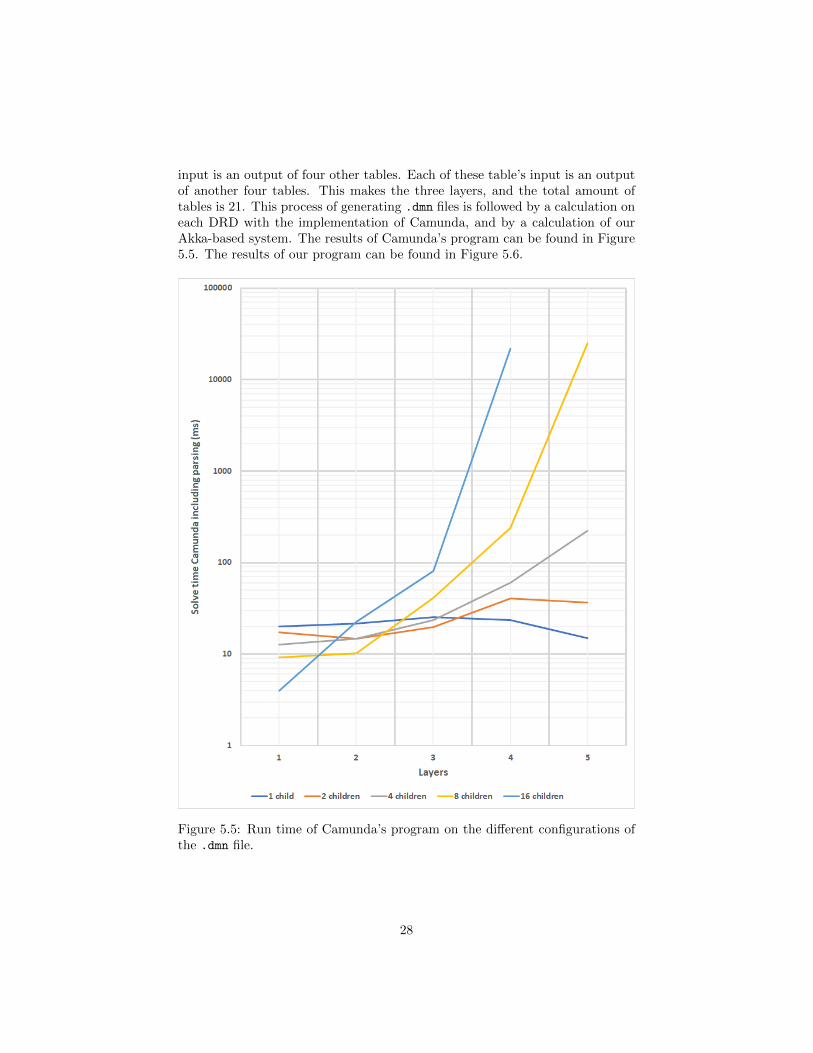
input is an output of four other tables. Each of these table’s input is an outputof another four tables. This makes the three layers, and the total amount oftables is 21. This process of generating .dmn files is followed by a calculation oneach DRD with the implementation of Camunda, and by a calculation of ourAkka-based system. The results of Camunda’s program can be found in Figure5.5. The results of our program can be found in Figure 5.6.

Figure 5.5: Run time of Camunda’s program on the different configurations ofthe .dmn file.

28

Figure 5.6: Run time of our program on the different configurations of the .dmn

file.

Evaluation of comparing these benchmarks With a few layers in theconfiguration, our program seems to be at least one order of magnitude faster.With more and more layers and children, this gap is only growing. The differenceon eight children and five layers is already two orders of magnitude. We abortedthe fifth layer with sixteen children on Camunda’s program, because we werealready waiting for half an hour. If the speed kept rising with the same speed,we calculated that the expected wait time was over five hours.

29

5.1.4 Speed comparison for different settings of actor model

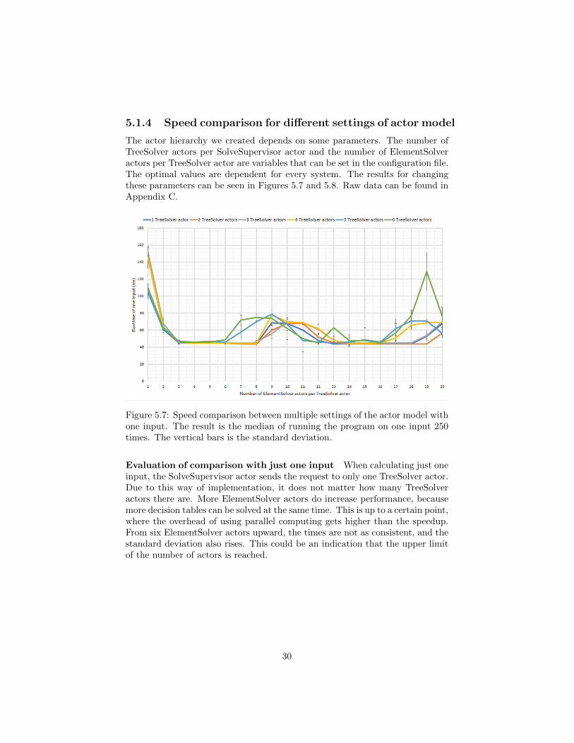
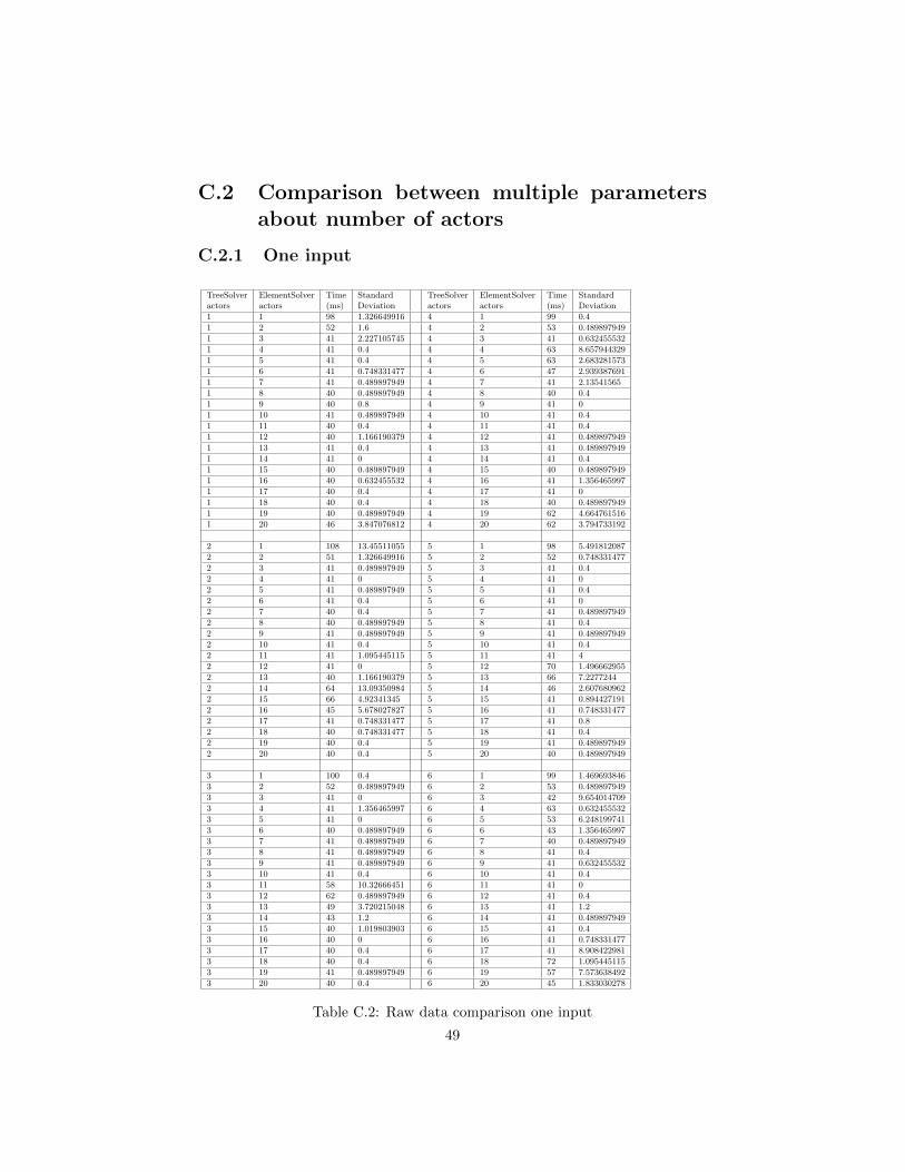
The actor hierarchy we created depends on some parameters. The number ofTreeSolver actors per SolveSupervisor actor and the number of ElementSolveractors per TreeSolver actor are variables that can be set in the configuration file.The optimal values are dependent for every system. The results for changingthese parameters can be seen in Figures 5.7 and 5.8. Raw data can be found inAppendix C.

Figure 5.7: Speed comparison between multiple settings of the actor model withone input. The result is the median of running the program on one input 250times. The vertical bars is the standard deviation.

Evaluation of comparison with just one input When calculating just oneinput, the SolveSupervisor actor sends the request to only one TreeSolver actor.Due to this way of implementation, it does not matter how many TreeSolveractors there are. More ElementSolver actors do increase performance, becausemore decision tables can be solved at the same time. This is up to a certain point,where the overhead of using parallel computing gets higher than the speedup.From six ElementSolver actors upward, the times are not as consistent, and thestandard deviation also rises. This could be an indication that the upper limitof the number of actors is reached.

30

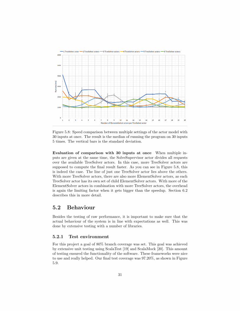
Figure 5.8: Speed comparison between multiple settings of the actor model with30 inputs at once. The result is the median of running the program on 30 inputs5 times. The vertical bars is the standard deviation.

Evaluation of comparison with 30 inputs at once When multiple in-puts are given at the same time, the SolveSupervisor actor divides all requestsover the available TreeSolver actors. In this case, more TreeSolver actors aresupposed to compute the final result faster. As you can see in Figure 5.8, thisis indeed the case. The line of just one TreeSolver actor lies above the others.With more TreeSolver actors, there are also more ElementSolver actors, as eachTreeSolver actor has its own set of child ElementSolver actors. With more of theElementSolver actors in combination with more TreeSolver actors, the overheadis again the limiting factor when it gets bigger than the speedup. Section 6.2describes this in more detail.

5.2 Behaviour

Besides the testing of raw performance, it is important to make sure that theactual behaviour of the system is in line with expectations as well. This wasdone by extensive testing with a number of libraries.

5.2.1 Test environment

For this project a goal of 80% branch coverage was set. This goal was achievedby extensive unit testing using ScalaTest [19] and ScalaMock [20]. This amountof testing ensured the functionality of the software. These frameworks were niceto use and really helped. Our final test coverage was 97.20%, as shown in Figure5.9.

31

Figure 5.9: Pipeline status and test coverage.

ScalaTest

ScalaTest is a framework that is designed to increase productivity through sim-ple, clear and readable tests that ensure correct functionality of code [19]. Al-most all tests in the project were written with ScalaTest which enabled everymember to write tests which are very easily understood by the rest of the team.

ScalaMock

For integration tests ScalaMock [20] was used. ScalaMock allowed the creationof dummy objects which are copies of objects which only allow certain calls toits methods, effectively testing whether another object makes the right methodcalls. In the beginning this was useful when testing components which usedfeatures which were not implemented yet, as these features could be mocked.When the features were implemented the tests could be replaced with unit-and integration tests. Mocks also proved to be useful when testing the entireproject at once. For example, when running a calculation, the Main object callsa printer object with the result and the printer object prints it to the console.This printer object can be mocked to add an expected result. When the Mainobject is done computing and it does not call the printer object with the correctresult the test fails.

TestKit

To test the actor system ScalaTest does not suffice. TestKit [21] enabled thetesting of individual actors to ensure that each actor behaved correctly in thebigger system.

5.3 Code quality

It is obvious that the code should work, and that that should be the first priority.But creating maintainable code is almost as important. This means that thecode should be of a high quality, adhering to the industry standards. The toolsand methods used to achieve these quality standards are listed below

Software Improvement Group

The Software Improvement Group, or SIG in short, checked the source codeand gave a detailed insight to improve the final code quality [22]. During ourproject, two checks were done by SIG. First in the sixth week, and a secondtime during the ninth week. The goal was to improve the quality of the code

32

base, based on the outcome of the first test. The second test is a check to see ifwhether the quality actually improved since the first test.

In the first test, the code base scored a 3.5 out of 5. Given feedback was thatsome methods had too much parameters, and the complexity of other methodswas too high. After receiving the feedback the issues were resolved almostimmediately and the settings for the other static analysis tools were changed sothey matched the SIG requirements for code quality.

Static code analysis

To improve the quality of the code besides the checks by SIG, static code analysistools were used. These tools checked the code without running it (thereforeit is static) in the CI pipelines and in the IDE itself. Immediately after thefirst feedback from SIG, we lowered the parameters for the warning on methodparameters and complexity. In this way, we had to use less parameters and writeless complex methods. This increases the overall quality and maintainability ofthe code.

Scaladoc

It is very important that the code is readable to other programmers that workwith the software in the future. For that reason, Scaladoc was added to allmethods and classes and, when needed, additional comments in methods wereadded.

5.4 Development Process

In the eight weeks of development the final product was implemented and a finalreport was written. Appendix A shows what was implemented each week. Thissection evaluates the development process and methods and lists the biggestproblems faced during development.

5.4.1 Scrum

To reach the final product, there were eight weeks of actual development. Touse these eight weeks as efficiently as possible, Scrum [23] was used. At thestart of each day a meeting was held to determine the activities of each memberthat day. For each activity an issue was added to the issue board on the GitLabrepository with an appropriate time estimate. When the activity was finished,the member could indicate the amount of time spend on that issue. This waythe time spend per week could be monitored to determine whether it was in linewith our expectations. The issue board also enables every one to keep track ofactivities of all other members.

This worked very well for us, because we always knew what to do next. Wecould assign ourselves a new issue. Sometimes at the end of the week, the issueswere not yet finished and had to shift to the sprint afterwards. Maybe this

33

would not be the case if we had sprints of two weeks, so next time we couldthink about that. We tracked our time for every issue, and that also workedvery well.

5.4.2 Git

For version control, Git [24] was used. Git allowed for a streamlined developmentprocess where each member could develop his feature separately in a branch ofthe master branch. When he was done he could create a pull request, whichhad to be approved by at least one other member, to merge his work back intothe master if the continuous integration tests succeeded. This ensured a clean,working and presentable master branch.

5.4.3 Continuous Integration

On every code push to the Git repository on the GitLab server, Continuous Inte-gration (CI) made sure that all specification tests and static code analysis toolswere ran in a pipeline. This way every member automatically knew whetherhis push was correct or faulty. CI also prevents the merging of faulty branchesinto the master. In the beginning of the project, the pipelines took a very longtime. This sometimes reduced our productivity because we had to wait for thepipeline to see if our change let the pipeline succeed. This was resolved after afew weeks. Therefore, in the end, the Continuous Integration worked perfectlyfor us.

5.4.4 Problems encountered during development

The main problem discovered during the project was the speed of the decisionengine. Camunda takes a very long time to solve when there is a high load andturned out to be very slow in reading DMN files. The plan was to use the parserof Camunda to read DMN files, however this turned out to be the bottleneck ofthe program. Parsing took more than half an hour when solving only took onlymilliseconds. Therefore the decision was made to not use Camunda at all andwrite a new DMN parser from scratch.

Another problem was the concurrency of the actors. The actors were sup-posed to work in parallel, such that the decision engine would increase in speed.However, the engine had the same performance with one actor as it had withany number of actors. The problem was that one method in an actor waited fora result of another actor, before the next task was sent. This way, only one actorwas working at the same time. When this was resolved, the problem occurredthat the actors took too much memory. To solve this we created a maximumnumber of tasks that can be solved at the same time. When those tasks aresolved the next batch of tasks are sent to the actors.

A very big challenge throughout the project was memory usage. When themaster actor had to handle a lot of requests at the same time, the system couldnot keep up and the requests would pile up and flood the available memory.

34

This issue was partly resolved at the time by re-implementing the TreeSolveractor to make it use less memory, but the problem resurfaced when anotherfix was implemented. This fix made sure that when the Master actor sent aparse request for a DRD to the Parser actors, it would not send another parserequest for that same DRD again while the Parser actor was still parsing. This,however, means that the Master actor had to keep all requests for that DRD inmemory. In the end the core cause of the problem was found with the JProfilersoftware. The cause was that, when a lot of requests were at the same time, theMaster actor would send a lot of solve requests in one go each of which containeda decision tree, which took a lot of space. Letting the TreeSolver actors fetchthe decision trees when they needed them resolved the issue.

We had a working decision engine very early in the development. We thenstarted to improve the performance using benchmarks and a profiler. When weare in the same situation in a future project, it could be a better idea to start anew research phase. Use a few days to sit together, and find out what the bestway is to improve the current system.

35

Chapter 6

Discussion andrecommendations

6.1 Results

When the .dmn file is already parsed, our program is about two orders of mag-nitude faster on calculating the output of a decision table than Camunda’sprogram. This means that you can give the program 100 times as many inputsas you can with Camunda’s program. When the parsing also gets involved, thedifference between the two programs is dependent on the size of the input. Butour program is at least one order of magnitude faster. Besides that, our pro-gram uses caching of parsed trees. Once the program has parsed the decisionrequirements diagram, the program will be as fast as Figure 5.3. Camunda’scode still needs to parse on every input, making it as fast as Figure 5.4. Thismakes our program three or more orders of magnitude faster than Camunda’sprogram on one decision tables.

On multiple decision tables, we only measured the performance of parsingand solving together. The difference is at least one order of magnitude, and isincreasing with more and more decision tables. This means that our programis even faster on larger DRDs compared to Camunda’s program than it is onsmaller DRDs. This shows that our program is more capable of handling biggerinput, which leads to a higher throughput.

6.1.1 Quality of the comparison

An analysis of the run time of a program is never 100% reliable. It is dependenton the systems resources (available memory, number of cores and threads, pro-cessor speed, etc.). A computer also performs tasks in the background, whichmakes the run time in the benchmark change on every run. Therefore we ran itmultiple times, and added an error bar, which represents the standard deviationof the multiple runs.

36

6.2 Bottleneck

Our program runs highly concurrent. The performance is therefore dependenton the system it runs on. It needs enough memory to keep the decision treescached, and larger DRDs leads to larger decision trees, and therefore also morememory needed. But the biggest factor is the number of threads the CPU has.Actors can work concurrently, but with more actors than available cores, someactors have to wait before they can process their messages. With more threads,more actors can work at the same time, resulting in even faster computationwith an even higher throughput.

6.3 Overhead of Akka

As specified in Section 2.3.2, using Ask messages gives some overhead. Thisresults in a longer run time. But nevertheless we used the Ask messages to senddata through our actor system. We started with using Ask messages becauseit seemed logical to use the ask-receive structure. The TreeSolver actors had towait for the result of the ElementSolver actors, which is perfectly handled in Askmessages. After some weeks, we wanted to improve the speed of the program.Therefore we wanted to change from Ask to Tell messages, as it should increaseperformance according to the Akka documentation [7]. This did not improvethe run time in our system on high loads. The TreeSolver actors did not knowwhen all the ElementSolver actors were ready, so it had nothing to wait for.Then the TreeSolver actors started with the next input to solve. This resultedin too many requests for the TreeSolver and ElementSolver actors to handleefficiently. Therefore we did not changed to Tell messages, and accepted thesmall overhead.

6.4 Future work

We did our best implementing as much as possible during our development, butof course it was not possible to implement everything. Below are some featuresthat could be implemented to extend the program in the future.

Newer DMN specifications When newer DMN specifications will be re-leased in the future, the program could be extended to be able to work withDRDs of that specification.

More extensive expression language Currently, the only expression lan-guage that is implemented is the FEEL expression, but only the part of FEELexpressions to make it work with the current DMN spec. The full FEEL expres-sion language is far more extensive, so this could all be implemented. Besidesthat, there are lots of other expression languages (JUEL for example) that couldbe implemented to extend the program even further.

37

Graphical user interface The program runs in the console, or on a serverwhere it can be accessed using an API. This could be extended with a graphicaluser interface (GUI) in the future. That will make the program easier to use,especially if users have less experience with using the program.

6.5 Ethical issues

In our project we developed a decision engine with the capability of evaluat-ing decisions in very large decision graphs, simultaneously, within a very smallamount of time. According to Theo SchlossNagle, CEO of Circonus, consideringethics, the one thing to ask yourself as a developer is: “How could this softwareharm someone?” [25]. For this software it would be easy to name a use case thatwould implicate harm due to its flexibility; it can be used to make decisions onliterally anything. The more important question to ask is whether the additionof this software specifically enables harm on individuals. This would only bethe case if this type of software did not exist before, which is not the case. Thistype of software already exists and therefore the addition of this project doesnot necessarily add to the possible harm of individuals.

38

Chapter 7

Conclusions

The main requirements for this project were to create a decision engine whichimplements the DMN specification, it should be callable by API, it should usethe Akka actor library as concurrency implementation, it should take a DMNfile name and input parameters as input and it should return the output valuesand a representation of the steps leading to that output. Furthermore, for thedevelopment process, the branch coverage by testing of the code base should begreater than 80%. Using benchmarks it was shown that the software createdin this project performs better than its Camunda counterpart and can handlevery high data loads. Furthermore, the code is tested for 97.20%. Therefore, ithas been shown that the main question of this project, “Is it possible to createa well tested decision engine for the DMN specification, using the Akka actorsystem, that performs very well on a very high load?”, has been answered and itis indeed feasible to create the software within the set time limits and accordingto development standards.

39

Bibliography

[1] Camunda. (2018) https://camunda.com. [Online]. Available: https://camunda.com

[2] Object Management Group, Decision Model and Notation Version 1.2,2019. [Online]. Available: https://www.omg.org/spec/DMN/1.2/PDF

[3] Wikipedia. (2019) The decision structure logic and data associated with theaccount verification. [Online]. Available: https://en.wikipedia.org/wiki/Decision Model and Notation#/media/File:DMNCertifyNewA DRG.jpg

[4] D. M. Solutions. (2016) An introduction to decision modeling withdmn. [Online]. Available: https://www.omg.org/news/whitepapers/AnIntroduction to Decision Modeling with DMN.pdf

[5] J. Purchase. (2018) A practitioner’s review of dmn 1.2. [Online]. Available:http://www.luxmagi.com/2018/06/a-practitioners-review-of-dmn-1-2/

[6] Camunda. (2019) Defaultdmndecisioncontext.java on 9-4-2019. [Online].Available: https://github.com/camunda/camunda-engine-dmn/blob/master/engine/src/main/java/org/camunda/bpm/dmn/engine/impl/DefaultDmnDecisionContext.java

[7] Akka. (2011) Akka: build concurrent, distributed, and resilient message-driven applications for java and scala — akka. [Online]. Available:https://akka.io/

[8] B. Storti. (2015) https://www.brianstorti.com/the-actor-model/. [Online].Available: https://www.brianstorti.com/the-actor-model/

[9] M. Gupta, Akka essentials. Packt Publishing Ltd, 2012.

[10] R. Neykova and N. Yoshida, “Multiparty session actors,” in InternationalConference on Coordination Languages and Models. Springer, 2014, pp.131–146.

[11] V. Pankratius, F. Schmidt, and G. Garreton, “Combining functional andimperative programming for multicore software: an empirical study evalu-ating scala and java,” in 2012 34th International Conference on SoftwareEngineering (ICSE). IEEE, 2012, pp. 123–133.

40

[12] JAX Editorial Team. (2016) 6 answers to the question: Whyscala and not java? [Online]. Available: https://jaxenter.com/expert-checklist-why-scala-and-not-java-129923.html

[13] J. Roper. (2012) Benchmarking scala against java. [Online]. Available:https://dzone.com/articles/benchmarking-scala-against

[14] A. Alexander. (2017) The differences between a scala future anda java thread. [Online]. Available: https://alvinalexander.com/scala/differences-java-thread-vs-scala-future

[15] Camunda. (2015) Editing dmn in camunda modeler. [Online]. Available:https://docs.camunda.org/manual/7.7/modeler/camunda-modeler/dmn/

[16] Oracle. (2019) Java garbage collection basics. [Online]. Avail-able: https://www.oracle.com/webfolder/technetwork/tutorials/obe/java/gc01/index.html

[17] E. Technologies. (2019) Jprofiler. [Online]. Available: https://www.ej-technologies.com/products/jprofiler/overview.html

[18] Haoyi. (2016) Benchmarking scala collections. [Online]. Available:http://www.lihaoyi.com/post/BenchmarkingScalaCollections.html

[19] artima. (2009) Scalatest. [Online]. Available: http://www.scalatest.org/

[20] ScalaMock. (2019) Scalamock. [Online]. Available: https://scalamock.org/

[21] Akka. (2011) Testing actor systems • akka documentation. [Online].Available: https://doc.akka.io/docs/akka/current/testing.html

[22] SIG. (2019) Sig — software improvement group. [Online]. Available:https://www.softwareimprovementgroup.com/

[23] Scrum. (2019) What is scrum? [Online]. Available: https://www.scrum.org/resources/what-is-scrum

[24] Git. (2019) About. [Online]. Available: https://git-scm.com/about

[25] B. L. InfoQ. (2018) Why software developers should take ethics intoconsideration. [Online]. Available: https://www.infoq.com/news/2018/03/software-developers-ethics/

[26] A. B. C. Limited. (2014) Moscow prioritisation. [Online]. Available:https://www.agilebusiness.org/content/moscow-prioritisation

41

Appendices

42

Appendix A

Weekly activities

A.1 Week 1 - Research

• Learned about Akka.• Learned how decision tables and decision requirement diagrams are scored

by Camunda.

A.2 Week 2 - Research

• Researched about the best way to create an actor system to score decisiontables and decision requirement diagrams.

• Created UML of the idea of the system.• Wrote research report about weeks 1 and 2.

A.3 Week 3 - Development

• Created classes according to the UML.• Communications between actors.• Read .dmn files, and parse them to decision trees.

A.4 Week 4 - Development

• Validated user input.• First running version which could calculate outputs on user input.• Cached decision trees for performance improvements.• Visualisation of trace of an output.

43

A.5 Week 5 - Development

• Fixed the calculation (wrong outcomes occurred).• Optimised messages between actors.• Created a .dmn file containing all possibilities to test the system.• Ability to automatically run and benchmark the system.

A.6 Week 6 - Development

• Refactored main class.• Improved performance (shorter runtime).• Upload to SIG.

A.7 Week 7 - Development

• Replaced foreach with while loops.• Replaced Camunda parser and FEEL expressions with our own code.• Wrote part of report.

A.8 Week 8 - Development

• Improved performance and memory usage using JProfiler.• Handled SIG feedback.• Created REST API.

A.9 Week 9 - Development

• Wrote part of report• Implemented parsing using actors• Further performance improvements using JProfiler

A.10 Week 10 - Development

• Finished report

A.11 Week 11 - Presentation

• Prepared and gave the final presentation.

44

Appendix B

MoSCoW

The MoSCoW method is a method to prioritise different requirements of the fi-nal product [26]. All items are classified under the labels ‘must’, ‘should’, ‘could’and ‘won’t’ have which specifies its priority. Because the project definition doesnot require a complicated user interface, but rather a simple API system, wedefine a single requirements list which focuses on the developer using the APIto create his own software.

B.1 Must haves

This sections contains all features that must be contained in the final product.

• The software must run continuously and return output on a given input

• The software must be callable by API

• The software must return outputs based on new inputs that are put inwhile the software is running

• The input to the API must be a combination of a Decision RequirementsGraph identifier and the input to that graph

• The code base must be tested as much as possible, with a minimum of80% branch coverage

B.2 Should haves

This section contains all features that should be contained in the final product,but have a lower priority than the must haves.

• The software should return a representation of the path taken through theDecision Requirement Diagram

• The software should give an appropriate error on corrupt decision models

45

• The software should be able to handle input and provide output to multipleDecision Requirement Diagrams at the same time

B.3 Could haves

This sections contains all features that could be in the final product, if there istime left.

• The software could contain a written parser for the DMN 1.2 spec .dmn

files

B.4 Won’t haves

This sections contains all features that will not be in the final product. Thosefeatures might be implemented in any future work.

• The software will not contain a user interface besides the API

• The software will not correct corrupt Decision Requirement Diagrams

• The software will not cache results to provide a speed up

Every bullet point will be divided in multiple sub-tasks, which will be theissues in the repository. There is no need to place all the sub-tasks in theMoSCoW, because that would make it only more unclear. Only the most im-portant features for a decision engine can be found in the MoSCow.

46

Appendix C

Speed comparison data

C.1 Benchmark between Camunda’s program andour program

Rules Camunda (ms)Camunda including

parsing (ms)Our implementation

(ms)Our implementation

including parsing (ms)

1 92 620 1 119

10 108 715 1 123

100 133 791 2 168

1,000 220 913 2 356

10,000 211 7,061 3 678

15,000 246 14,323 4 792

20,000 268 21,010 13 925

25,000 279 39,770 14 921

30,000 357 95,379 17 1,004

35,000 311 91,906 5 1,024

40,000 375 124,810 8 1,071

45,000 341 170,350 13 1,160

50,000 374 213,977 9 1,174

60,000 646 283,823 8 1,629

70,000 469 513,800 10 1,772

80,000 11 1,975

90,000 11 1,860

100,000 15 2,578

200,000 22 6,118

300,000 33 9,406

500,000 58 17,299

Table C.1: Raw benchmark data

47

48

C.2 Comparison between multiple parametersabout number of actors

C.2.1 One input

TreeSolveractors

ElementSolveractors

Time(ms)

StandardDeviation

TreeSolveractors

ElementSolveractors

Time(ms)

StandardDeviation

1 1 98 1.326649916 4 1 99 0.4

1 2 52 1.6 4 2 53 0.489897949

1 3 41 2.227105745 4 3 41 0.632455532

1 4 41 0.4 4 4 63 8.657944329

1 5 41 0.4 4 5 63 2.683281573

1 6 41 0.748331477 4 6 47 2.939387691

1 7 41 0.489897949 4 7 41 2.13541565

1 8 40 0.489897949 4 8 40 0.4

1 9 40 0.8 4 9 41 0

1 10 41 0.489897949 4 10 41 0.4

1 11 40 0.4 4 11 41 0.4

1 12 40 1.166190379 4 12 41 0.489897949

1 13 41 0.4 4 13 41 0.489897949

1 14 41 0 4 14 41 0.4

1 15 40 0.489897949 4 15 40 0.489897949

1 16 40 0.632455532 4 16 41 1.356465997

1 17 40 0.4 4 17 41 0

1 18 40 0.4 4 18 40 0.489897949

1 19 40 0.489897949 4 19 62 4.664761516

1 20 46 3.847076812 4 20 62 3.794733192

2 1 108 13.45511055 5 1 98 5.491812087

2 2 51 1.326649916 5 2 52 0.748331477

2 3 41 0.489897949 5 3 41 0.4

2 4 41 0 5 4 41 0

2 5 41 0.489897949 5 5 41 0.4

2 6 41 0.4 5 6 41 0

2 7 40 0.4 5 7 41 0.489897949

2 8 40 0.489897949 5 8 41 0.4

2 9 41 0.489897949 5 9 41 0.489897949

2 10 41 0.4 5 10 41 0.4

2 11 41 1.095445115 5 11 41 4

2 12 41 0 5 12 70 1.496662955

2 13 40 1.166190379 5 13 66 7.2277244

2 14 64 13.09350984 5 14 46 2.607680962

2 15 66 4.92341345 5 15 41 0.894427191

2 16 45 5.678027827 5 16 41 0.748331477

2 17 41 0.748331477 5 17 41 0.8

2 18 40 0.748331477 5 18 41 0.4

2 19 40 0.4 5 19 41 0.489897949

2 20 40 0.4 5 20 40 0.489897949

3 1 100 0.4 6 1 99 1.469693846

3 2 52 0.489897949 6 2 53 0.489897949

3 3 41 0 6 3 42 9.654014709

3 4 41 1.356465997 6 4 63 0.632455532

3 5 41 0 6 5 53 6.248199741

3 6 40 0.489897949 6 6 43 1.356465997

3 7 41 0.489897949 6 7 40 0.489897949

3 8 41 0.489897949 6 8 41 0.4

3 9 41 0.489897949 6 9 41 0.632455532

3 10 41 0.4 6 10 41 0.4

3 11 58 10.32666451 6 11 41 0

3 12 62 0.489897949 6 12 41 0.4

3 13 49 3.720215048 6 13 41 1.2

3 14 43 1.2 6 14 41 0.489897949

3 15 40 1.019803903 6 15 41 0.4

3 16 40 0 6 16 41 0.748331477

3 17 40 0.4 6 17 41 8.908422981

3 18 40 0.4 6 18 72 1.095445115

3 19 41 0.489897949 6 19 57 7.573638492

3 20 40 0.4 6 20 45 1.833030278

Table C.2: Raw data comparison one input

49

C.2.2 30 inputs at the same time

TreeSolveractors

ElementSolveractors

Total time(ms)

StandardDeviation

TreeSolveractors

ElementSolveractors

Total time(ms)

StandardDeviation

1 1 3115 157.8751405 4 1 1925 35.13175202

1 2 1696 88.70941325 4 2 1804 49.49989899

1 3 1387 95.26888264 4 3 1571 225.1092179

1 4 1372 75.35940552 4 4 1253 68.8168584

1 5 1350 107.3256726 4 5 1162 102.4304642

1 6 1353 61.06848614 4 6 1075 35.64828187

1 7 1368 71.60614499 4 7 1051 22.22071106

1 8 1345 50.31659766 4 8 995 111.479146

1 9 1343 82.25958911 4 9 1035 18.26909959

1 10 2094 47.9124201 4 10 1030 87.20917383

1 11 1995 272.6550935 4 11 1003 51.30847883

1 12 1533 182.0213174 4 12 1041 29.15887515

1 13 1319 102.3824204 4 13 1065 101.8744325

1 14 1365 60.89334939 4 14 1219 79.72603088

1 15 1352 49.46352191 4 15 1667 186.3866948

1 16 1357 74.50208051 4 16 1797 73.40681167

1 17 1328 107.1156384 4 17 1844 132.9249412

1 18 1345 128.3853574 4 18 1345 86.14545838

1 19 1335 36.75323115 4 19 1176 54.81751545

1 20 1362 75.34825811 4 20 1129 108.3653081

2 1 1946 326.0813395 5 1 1088 85.97301902

2 2 2019 157.7156936 5 2 1014 87.77607875

2 3 1725 25.3424545 5 3 948 33.31906361

2 4 1422 224.1228235 5 4 989 41.11447434

2 5 1231 55.95140749 5 5 970 82.89607952

2 6 1163 25.99692289 5 6 1015 15.64097184

2 7 1089 85.20187791 5 7 1072 89.39932886

2 8 1134 88.25780419 5 8 1050 79.56531908

2 9 1137 38.13135193 5 9 1241 62.50439985

2 10 1149 39.97199019 5 10 1770 174.2389164

2 11 1095 36.69550381 5 11 1773 68.44559884

2 12 1122 95.79686842 5 12 1771 128.0599859

2 13 1098 28.38027484 5 13 1314 62.20096462

2 14 1344 58.1914083 5 14 1180 68.75463621

2 15 1681 202.7721874 5 15 1074 84.25769994

2 16 1838 42.04759208 5 16 999 13.39253523

2 17 1594 134.3541588 5 17 1053 150.3821798

2 18 1248 67.79085484 5 18 1038 34.48477925

2 19 1191 103.2763284 5 19 1040 26.39242316

2 20 1092 33.35026237 5 20 1018 127.825819

3 1 1176 111.6913605 6 1 1035 29.53235514

3 2 1030 31.98499648 6 2 982 141.5302088

3 3 1045 93.28665499 6 3 1095 51.02783554

3 4 1005 22.60619384 6 4 1310 102.1203212

3 5 1105 99.41549175 6 5 1694 58.32117969

3 6 1267 63.59056534 6 6 1637 48.31148932

3 7 1646 234.9788076 6 7 1685 211.1681794

3 8 1813 49.02815518 6 8 1191 39.95197117

3 9 1651 170.9580065 6 9 1072 66.26190459

3 10 1259 62.28322407 6 10 1052 109.5945254

3 11 1141 117.7583967 6 11 1040 26.45297715

3 12 1116 72.95313564 6 12 933 138.6584292

3 13 1034 52.02076508 6 13 995 19.77270846

3 14 1071 59.79765882 6 14 1042 53.54026522

3 15 1113 62.11151262 6 15 976 66.80419149

3 16 1051 140.2192569 6 16 1008 41.87409701

3 17 1057 30.92830419 6 17 985 106.6819572

3 18 1110 105.2760182 6 18 1035 61.52852997

3 19 1140 81.43316278 6 19 1336 234.7369592

3 20 1358 78.77715405 6 20 1668 60.90451543

Table C.3: Raw data comparison 30 inputs at the same time

50