Aircraft three-dimensional hard- constrained trajectory ...

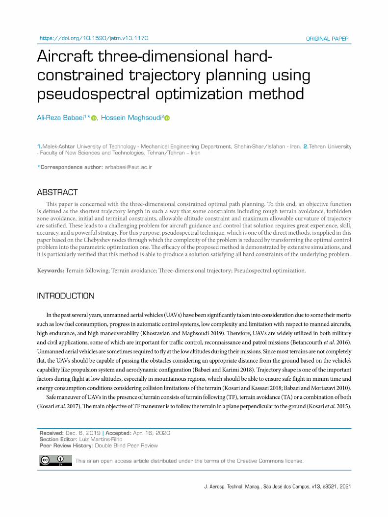
J. Aerosp. Technol. Manag., São José dos Campos, v13, e3521, 2021

https://doi.org/10.1590/jatm.v13.1170 ORIGINAL PAPER

ABSTRACTThis paper is concerned with the three-dimensional constrained optimal path planning. To this end, an objective function

is defined as the shortest trajectory length in such a way that some constraints including rough terrain avoidance, forbidden zone avoidance, initial and terminal constraints, allowable altitude constraint and maximum allowable curvature of trajectory are satisfied. These leads to a challenging problem for aircraft guidance and control that solution requires great experience, skill, accuracy, and a powerful strategy. For this purpose, pseudospectral technique, which is one of the direct methods, is applied in this paper based on the Chebyshev nodes through which the complexity of the problem is reduced by transforming the optimal control problem into the parametric optimization one. The efficacy of the proposed method is demonstrated by extensive simulations, and it is particularly verified that this method is able to produce a solution satisfying all hard constraints of the underlying problem.

Keywords: Terrain following; Terrain avoidance; Three-dimensional trajectory; Pseudospectral optimization.

Aircraft three-dimensional hard-constrained trajectory planning using pseudospectral optimization methodAli-Reza Babaei1* , Hossein Maghsoudi2

1.Malek-Ashtar University of Technology - Mechanical Engineering Department, Shahin-Shar/Isfahan - Iran. 2.Tehran University - Faculty of New Sciences and Technologies, Tehran/Tehran – Iran

*Correspondence author: [email protected]

INTRODUCTION

In the past several years, unmanned aerial vehicles (UAVs) have been significantly taken into consideration due to some their merits such as low fuel consumption, progress in automatic control systems, low complexity and limitation with respect to manned aircrafts, high endurance, and high maneuverability (Khosravian and Maghsoudi 2019). Therefore, UAVs are widely utilized in both military and civil applications, some of which are important for traffic control, reconnaissance and patrol missions (Betancourth et al. 2016). Unmanned aerial vehicles are sometimes required to fly at the low altitudes during their missions. Since most terrains are not completely flat, the UAVs should be capable of passing the obstacles considering an appropriate distance from the ground based on the vehicle’s capability like propulsion system and aerodynamic configuration (Babaei and Karimi 2018). Trajectory shape is one of the important factors during flight at low altitudes, especially in mountainous regions, which should be able to ensure safe flight in minim time and energy consumption conditions considering collision limitations of the terrain (Kosari and Kassaei 2018; Babaei and Mortazavi 2010).

Safe maneuver of UAVs in the presence of terrain consists of terrain following (TF), terrain avoidance (TA) or a combination of both (Kosari et al. 2017). The main objective of TF maneuver is to follow the terrain in a plane perpendicular to the ground (Kosari et al. 2015).

Received: Dec. 6, 2019 | Accepted: Apr. 16, 2020Section Editor: Luiz Martins-FilhoPeer Review History: Double Blind Peer Review

This is an open access article distributed under the terms of the Creative Commons license.


Babaei A-R, Maghsoudi H2

Since this trajectory is implemented in the vertical plane, TF is a two-dimensional problem, hence, only the longitudinal dynamics of the flying vehicle is included (Kamyar and Taheri 2014). However, the TA maneuver is accomplished in a horizontal plane in which the air vehicle flies at the low altitudes without the terrain collision. In the most real cases, the two above-mentioned maneuvers are usually combined as a TF/TA maneuver in which the vehicle should fly over the mountains, turn the obstacles with the constant altitude or accomplish both of them so that we encounter with a hard problem. Therefore, the main objective of this problem is moving toward the target in a three-dimensional space without terrain collision, so that an objective function including flight time, flight trajectory length, energy consumption and so forth is optimized (Celis et al. 2014). Besides, it should be mentioned that the problem is complicated by considering the dynamical constraints like maximum curvature of trajectory and kinematics constraints such as maximum altitude and flight path angle. Therefore, trajectory planning is a challenging problem due to the presence of these constraints.

Several researches have been performed to solve this problem, which is known as trajectory optimization problem or trajectory planning. Huang et al (2012), Conway (2012), Betts (2010), Rao (2009), and Vittorio and Bernardino (2004) presented a comprehensive review of the studied researches related to the optimal trajectory planning. Optimal control and classical optimization methods have been led to some techniques which are so practical in the trajectory planning problems. In these approaches, different equality and inequality constraints can be included in the problem. Numerical techniques have also been employed for solving the optimal control problems. These techniques are divided into two major categories including direct and indirect techniques (von Stryk and Bulirsch 1992; Grimm and Hiltmann 1987).

Indirect numerical methods are based on the calculation of variations in which the optimal control problem is finally transformed into a Hamiltonian boundary-value problem (HBVP). Note that the numerical approximation methods are employed for solving the HBVP. Although the indirect methods have some merits, such as high accuracy, they suffer from the following disadvantages (Benson et al. 2006):• Indirect methods need to extract the optimality conditions analytically. In most cases, this is time-consuming and leads to

difficulties in problem solving.• These methods need an initial guess of the costate variables, which is very complicated because there is no physical sense

from the costate variables.• Domain of convergence in these methods is low as well as computational speed is not satisfactory.

Indirect methods first provide the necessary and sufficient conditions for the optimization and then attempt to discretize these conditions and solve them numerically. A common way to differentiate between these two methods is that in the direct method discretization takes place before optimization, while in the indirect method the optimization takes precedence over discretization (Kelly 2017; Kosari et al. 2017).

The main advantage of the indirect method over the direct approach is that it is generally more accurate. Moreover, it offers more reliable error estimation. Both of these benefits are due to the analytical expressions related to the necessary and sufficient conditions that the user derives when indirectly approaches the problem (Kelly 2017).

There are several limitations associated with the indirect methods compared to the direct ones. For instance, the convergence region is smaller in indirect methods, which requires better initialization. Besides, the initialization in the indirect method is a more complicated process because of the need to initialize the adjoint variables. On the contrary, these variables (and their initialization) do not exist in the direct approaches. Finally, it is worthwhile to mention that it is necessary to derive the required necessary and sufficient conditions analytically to achieve an accurate solution through an indirect approach, which can be usually a challenging process (Kelly 2017; Kosari et al. 2017).

In direct methods, the optimal control problem is transformed into a nonlinear programming problem (NLP) with bounded dimensions. There are two techniques for transformation, one of which is discretization through numerical integration or differentiation equations, and another is the application the parameterization methods (Garg 2011; Garg et al. 2011; Navabi et al. 2008; Fahroo and Ross 2008; Elnagar et al. 1995). Since it is not required to employ the initial guess and optimality conditions in the direct methods, these techniques are far more effective in comparison with the indirect methods. However, the accuracy of the indirect methods is higher than the direct ones. There are numerous direct methods for solving the optimization problems, one of which is the pseudospectral method, which is commonly preferred due to its high accuracy as well as convergence rate (Garg 2011). In pseudospectral parameterization methods, polynomials are employed for approximating the continuous time-dependent functions associated with the state and control variables. Chebyshev nodes with Lagrange polynomials can be applied in the pseudospectral parameterization method. In other words, by utilizing the direct pseudospectral method, the optimal control problem is transformed into a nonlinear programming that is solved via developed algorithms (Sakode and Padhi 2018; Shen et al. 2016; Sagliano et al. 2016; Kim and Melton 2014).


Aircraft three-dimensional hard-constrained trajectory planning using pseudospectral optimization method 3

Garg (2011) proposed a direct transcription technique, namely the Radau pseudospectral method (RPM), in which the global Lagrange polynomials and Legendre-Gauss-Radau (LGR) are respectively utilized to estimate control and state variables, and select the node points. The mentioned method in Garg (2011) was employed by Garg et al. (2011) to solve infinite-horizon optimal control problems. It was also used by Mashadi and Majidi (2014) to solve two-phase optimal path planning of autonomous ground vehicles. Vlassenbroeck (1988) and Vlassenbroeck and Dooren (1988) used the pseudospectral techniques using Chebyshev polynomials to solve the nonlinear optimal control problems, such as the orbit transfer problem. In Elnagar et al. (1995), and Elnagar and Razzaghi (1997), the pseudospectral method was developed via Lagrange polynomials and Legendre-Gauss-Lobatto (LGL) collocation points through which the nonlinear optimal control problems can be solved considering the variables limitations. Fahroo and Ross (2002; 2008( dedicated their researches to the pseudospectral method based on the developed Legendre, which is widely utilized to estimate the costate variables during the solution of optimal control problems. The aforementioned technique was later known as Lobatto pseudospectral method (LPM). Biegler and Zavala (2009) and Benson (2005) presented another Legendre-based pseudospectral approach, namely Gauss pseudospectral method (GPM), in which Lagrange polynomials and Legendre-Gauss (LG) points are employed for the basic functions and collocation, respectively.

The main objective of this paper was to generate the optimal trajectories for UAVs using direct pseudospectral method under the following specifications:• The flight environment contains the three-dimensional rough terrain and forbidden zone in which the obtained flight

trajectory should be capable of meeting the TA criterion without passing the forbidden zone.• Flight trajectory has minimum and maximum altitude limitations relative to the ground. These constraints are defined for

terrain avoidance and escaping from the radar coverage, respectively.• Flight trajectory has the maximum curvature limitation due to the dynamical constraints.• There are initial and terminal constraints according to the mission requirements.• The objective function is considered to achieve the shortest trajectory.• In presence of prior knowledge terrain, it is assumed that the problem is solved as offline.

The above specifications lead to a hard problem for aircraft guidance and control, so that it has created an attractive research field in flight trajectory planning.

PROBLEM FORMULATION

As already mentioned, the main objective of this paper is to plan an optimal trajectory for UAVs, so that some constraints such as terrain obstacles, forbidden zone and dynamical/kinematical constraints are met. Therefore, objective function and constraints of the problem are first defined.

Objective functionIn general, the cost function in each optimization problem can be selected based on the shortest trajectory length, minimum

flight time, minimum fuel consumption, minimum control effort and so forth. In this paper, it is strived to obtain a trajectory between initial and terminal points in such a way that the acquired path would be the shortest possible trajectory. The shortest trajectory length cost function is defined as follows (Eq. 1):

(1)

where X = (x, y, z) are the position vector of the aircraft that will be described by Lagrange polynomials. Other cost functions, such as minimum flight time and minimum fuel consumption, can be applied.

Boundary condition constraintIn each optimal control problem, the initial and terminal conditions for state variables are defined as follows (Eqs. 2 and 3):

(2)



(3)

where ψ0 and ψf are the initial and final constraint functions at the start and end times (τ0, τf), respectively, that they are constrained by ψ0 and ψf. It should be noted that these constraints can be either linear or nonlinear based on the type of problem. Here, the initial and terminal conditions for the trajectory planning problem are defined as follows (Eqs. 4 and 5):

(4)

(5)

where α0 is the angle between the horizontal projection of the velocity vector and x-axis of reference frame, and β0 is the angle between the velocity vector and Z-axis of the reference frame. These angles are shown in Fig. 1. As shown in Fig. 2, given the unit vector along the takeoff velocity, the takeoff angles can be calculated based on the following relationships:

(6)

(7)

Z

X

YStart

Goal

α

β

Figure 1. Initial and terminal conditions of the flight trajectory.

z

x

ya2j

a3k

(a1, a2, a3)

a1i

a

j0

k

i

α

β

Figure 2. Takeoff velocity vector and its angles.



Dynamic constraintThere are trajectory constraints in each trajectory planning problem, as noted below (Eq. 8):

(8)

where Φ is the constraint vector during the trajectory, and can be defined as either linear or nonlinear algebraic equations. Moreover, Φu and Φl are the upper and lower limitations, respectively.

There are numerous constraints during trajectory planning process, one major category being the physical constraints. One of the most important physical constraints is the capability of the flying vehicle during its maneuvering in such a way that the vehicle would not be capable to accomplish the turn and pull up/down maneuvers with each arbitrary rate. Since these maneuvers are limited based on the vehicle’s dynamics, the trajectory curvature constraint should be imposed on the problem. To impose the aforementioned constraint, the trajectory radius should not be lower than a minimum value (Rmin). The trajectory radius can be calculated by using curvature equations in the three-dimensional Cartesian coordinate system as follows in Eqs. 9 and 10:

(9)

(10)

where R(τ) and K(τ) are radius and curvature of the trajectory, respectively. Schematically, curvature of trajectory has been shown in Fig. 3. The following relationships are employed for calculating K(τ) in the three-dimensional Cartesian coordinate system (Eqs. 11–13):

(11)

(12)

(13)

C

R

P

Figure 3. Schematic curvature of the trajectory.

Forbidden zone constraintAs another constraint, the forbidden zone is considered in this paper as follows (Eq. 14):

(14)



where XFZ and YFZ are the coordinates of the center of the forbidden zone. Moreover, RFZ is the radius of the forbidden zone. Note that the forbidden zone has been defined as a cylinder with a specified radius and infinite height, and a schematic of them is in Fig. 4.

y

x

z

Goal

Start

Flight Path

Forbidden Zone

Forbidden Zone

Forbidden Zone

Forbidden Zone

Figure 4. Schematic of the forbidden zone along with the flight path.

Obstacle avoidance constraintThe following constraints are defined for the purpose of obstacle or terrain collision avoidance (Eqs. 15 and 16):

(15)

(16)

where, hTerrain (X(τ), Y(τ)) is the terrain altitude and hmin and hmax are the minimum and maximum clearance with respect to terrain, respectively, as shown in Fig. 5. Beside the presented constraints, these requirements lead to the full challenging problem.

hmin

Terrain

hmax

Figure 5. Schematic of the minimum and maximum altitudes with respect to the terrain.

The complexity of gradient-based optimization methods depends on the volume and difficulty of constraints. Therefore, the challenges appear when the constraints are enlarged and complicated.

PROBLEM SOLUTION: PSEUDOSPECTRAL METHOD

This section explains how pseudospectral method is utilized for trajectory planning problem described in the previous section. To apply pseudospectral method, the problem should be first parameterized in such a way that the problem is transformed into a nonlinear programming problem. Therefore, the obtained trajectory contains a set of discrete nodes between initial and terminal



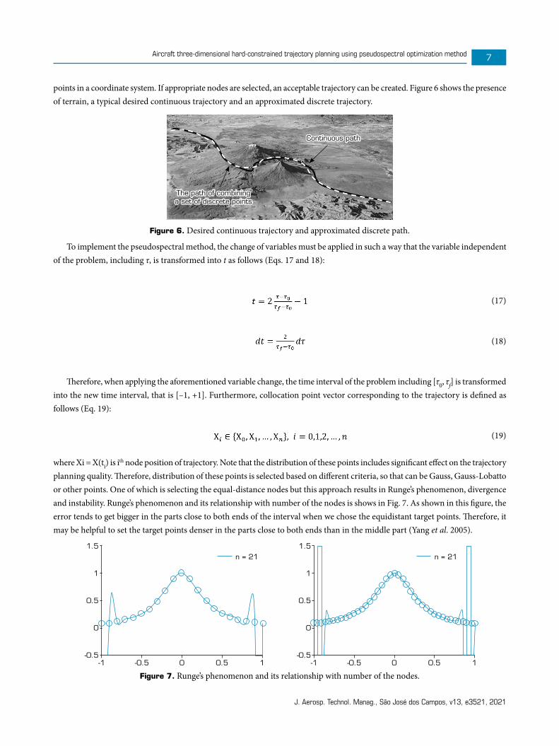
points in a coordinate system. If appropriate nodes are selected, an acceptable trajectory can be created. Figure 6 shows the presence of terrain, a typical desired continuous trajectory and an approximated discrete trajectory.

Continuous pathContinuous path

The path of combining The path of combining a set of discrete pointsa set of discrete points

Figure 6. Desired continuous trajectory and approximated discrete path.

To implement the pseudospectral method, the change of variables must be applied in such a way that the variable independent of the problem, including τ, is transformed into t as follows (Eqs. 17 and 18):

(17)

(18)

Therefore, when applying the aforementioned variable change, the time interval of the problem including [τ0, τf] is transformed into the new time interval, that is [–1, +1]. Furthermore, collocation point vector corresponding to the trajectory is defined as follows (Eq. 19):

(19)

where Xi = X(ti) is ith node position of trajectory. Note that the distribution of these points includes significant effect on the trajectory planning quality. Therefore, distribution of these points is selected based on different criteria, so that can be Gauss, Gauss-Lobatto or other points. One of which is selecting the equal-distance nodes but this approach results in Runge’s phenomenon, divergence and instability. Runge’s phenomenon and its relationship with number of the nodes is shows in Fig. 7. As shown in this figure, the error tends to get bigger in the parts close to both ends of the interval when we chose the equidistant target points. Therefore, it may be helpful to set the target points denser in the parts close to both ends than in the middle part (Yang et al. 2005).

1.5

1

0.5

0

-0.5

1.5

1

0.5

0

-0.5-1 -1-0.5 -0.50 00.5 0.5

n = 21 n = 21

1 1

Figure 7. Runge’s phenomenon and its relationship with number of the nodes.



According to Fig. 7, there are frequent fluctuations near the borders when using “equidistant points” method for interpolation. Also, a greater number of collocation points leads to more error in interpolation. This phenomenon may be solved by using Chebyshev nodes. Chebyshev nodes can be used to minimize the interpolation error and fluctuations near borders. According to the Chebyshev method, the distribution of nodes is selected to achieve the acceptable convergence as well as computational stability. For example, this fact is illustrated in Figs. 8 and 9. In these examples, the polynomial approximations for y = 1/(1 + 12s2) based on 11 equally spaced nodes and Chebyshev nodes over [–1, 1] have been shown.

-1 -0.8 -0.6 -0.4 -0.2 0 0.2 0.4 0.6 0.8 1

1.5

1

0.5

0

-0.5

Real data (y)

The polynomial approximation to y based on 11 eqyally spaced nodes

Collocation Points to equally spaced nodes

Figure 8. The polynomial approximation to y = 1/(1 + 12s2) based on 11 equally spaced nodes over [–1, 1].

-1 -0.8 -0.6 -0.4 -0.2 0 0.2 0.4 0.6 0.8 1

1.5

1

0.5

0

-0.5

Real data (y)

The polynomial approximation to y based on 11 Chebyshev nodes

Collocation Points to equally spaced nodes

Figure 9. The polynomial approximation to y = 1/(1 + 12s2) based on 11 Chebyshev nodes over [–1, 1].

Based on the Chebyshev method, a possible choice for nodes is the projection of the equidistant points on the circle centered at the middle point of the interval along the t axis. Finally, the nodes can be obtained as follows (Eq. 20) (Yang et al. 2005):

(20)

From the geometrical point of view, these nodes are projection of n = 1 points determined with the angular distances of (2n + 1– 2k)π/(2n + 2) on the boundary of a half-circle with the radius 1 on the horizontal axis, which are depicted in Fig. 10 for n = 4.



Chebyshev nodes

1

0-1

x0 = cos(9π/10) x0 = cos(7π/10) x0 = cos(5π/10) x0 = cos(3π/10) x0 = cos(π/10)

-0.8 -0.6 -0.4 -0.2 0 0.2 0.4 0.6 0.8 1

Figure 10. Chebyshev nodes for n = 4.

In the pseudospectral method, the gth state variable is approximated as below (Eq. 21):

(21)

where n is the number of nodes. L1(t) stands for the ti basis function. Moreover, ti denotes the ith discretization point associated with the gth state variable Xg(ti). In this paper, Lagrange basis functions that are considered for modeling variables, are formulated as follows (Eq. 22):

(22)

which meet the Kronecker delta criterion, meaning that:

(23)

To follow the curvature constraint, the first- and second-order differentials of the path have to be calculated, respectively, as below (Eqs. 24–27):

(24)

(25)

(26)

(27)



After applying the appropriate substitutions, the initial, final and path constraints and the recast cost function are, respectively, as follows (Eqs. 28–31):

Initial constraints:

(28)Final constraints:

(29)Path constraints:

(30)Cost function:

(31)

To deal with the possible integral terms included in the cost function, the quadrature can be used, which estimates the value associated with the integral of a function based on its own value in some given points, as shown in Eq. 32:

(32)

where Wi is the ith weight of the quadrature. In fact, a quadrature rule is an approximation of the definite integral of a function, stated as a weighted sum of function values at specified points within the domain of integration. By suitable choosing both the weights and the evaluation points, the accuracy of the integral can be improved. The ith weight of the quadrature is defined in a short form as follows (Eq. 33):

(33)

therefore,

(34)

The above quadrature has n+1 nodes. After parameterization and elimination of the differential constraints, the optimal control problem is converted to an NLP. The pseudospectral method recasts the problem as a static optimization problem, for whose solution optimal values of the states in the nodes must be obtained, minimizing the cost function and satisfying the constraints. To this end, NLP solvers, such as SNOPT, NPSOL, IPOPT and FMINCON, may be used.

SIMULATION RESULTS

In the previous sections, the algorithm of safe and optimal trajectory planning for a UAV based on the pseudospectral method was explained. Thereafter, the algorithm is challenged by applying it on a hard-constrained example. To represent a complex example, it is tried that models of terrain be generated close to real-world terrains (Zagros Mountain DEM). The objective of this simulation is to find a safe trajectory for a UAV, so that the UAV can track it and not collide with the terrain. The forbidden zone is modeled by an infinite-altitude cylindrical domain that constrains the trajectory to be outside this region. It is worthwhile to mention that UAVs cannot maneuver arbitrarily because of the constraints in their dynamical nature. In other words, the trajectory resulting



from the simulation must be consistent with the vehicle’s dynamics so that at different flight speeds the vehicle has the capability to maneuver accordingly and thus avoid damage. This design consideration was applied in the simulation with a restriction in the radius of curvature of the trajectory.

Corresponding to values presented in Table 1, Figs. 11 to 14 present the results of the simulation, which confirm the validity of the proposed procedure for trajectory planning in presence of rough three-dimensional terrain obstacles and forbidden zones.

Table 1. The values of the constraints and physical parameters.

ValuePhysical constraints

(x(–1), (y(–1), (z(–1) = (1500, 1600, 54.6)The initial (takeoff) position (m)

(x(+1), (y(+1), (z(+1) = (9050, 570, 400)The final (landing) position (m)

(xFZ, yFZ) = (6140, 918)The origin of the forbidden zone (m)

RFZ = 150The radius of the forbidden zone (m)

hmax = 170The maximum altitude with respect to the terrain obstacles (m)

hmin = 30The minimum altitude with respect to the terrain obstacles (m)

Rmin = 150The minimum radius of the path (m)

α–1 = 8, β–1 = 75The initial (takeoff) angles of the path (deg)

3000

100009000

80007000

60005000

40003000

20002000

10001000

0

0

Alti

tude

(m

)

Downrange (m)

Figure 11. Generated three-dimensional trajectory in presence of rough terrain and forbidden zone.

2000

800

600

400

200

0

TrajectoryTerrainMaximum AltitudeInitial PointFinal Point

3000 4000 5000 6000Down Range (m)

Alti

tude

(m

)

7000 8000 9000

Figure 12. Vertical trajectory in presence of rough terrain and forbidden zone.



TrajectoryTerrainInitial PointFinal Point

400

200

0Alti

tude

(m

)

Cro

ss R

ange

(m

)

10000 9000 8000 7000 6000 5000 4000 3000 2000 1000

1500

500

1000

Figure 13. The three-dimensional optimal trajectory and terrain profile.

8000

6000

4000

2000

1500

1000

500

500

250

0

-1

-1

-1

-0.8

-0.8

-0.8

-0.6

-0.6

-0.6

-0.4

-0.4

-0.4

-0.2

-0.2

-0.2

0

0

0

0.2

0.2

0.2

0.4

0.4

0.4

.06

.06

.06

0.8

0.8

0.8

1

1

1

Dow

n R

ange

(m

)Cro

ss R

ange

(m

)Alti

tude

(m

)

Collocation Points

Figure 14. Collocation points for generated trajectory.

From the simulation results, it can be inferred that:• The solution returned by NLP solvers depends on the initial guess, so it is crucial to make an appropriate initial estimation.

As the desired path closely resembles the straight line connecting the start and end points, it might be helpful to consider the points lying on the foregoing line as the initial guesses.

• Although the computational efficiency and the quality of the solution directly relate to the number of the nodes, considering an unreasonable number of the nodes leads to divergence. Therefore, choosing larger number of the nodes for complex problems, and fewer ones for simpler problems, is recommended. Before implementing the algorithm, there is not any definite answer to the question that how many nodes should be taken into account? In this paper, 35 nodes are considered. Besides, for complex problem that imposes the large number of nodes the pseudospectral-based trajectory has some fluctuations.

• As indicated by the simulation results, the solution has to minimize the length of the path and meet the constraints, so the generated path tends to resemble the straight line connecting the start and end points. Moreover, it automatically prefers vertical maneuvers by TF, unless in the case of facing very high obstacles and forbidden zone. This conclusion is confirmed by other approaches as well.



• Although the applied method solved the presented problem, but constraints and conditions change led to other try and error procedure for solver setting such as number of nodes. The number of nodes is a parameter for correcting the trajectory planning algorithm results.

CONCLUSION

The main objective of this paper is an optimal three-dimensional path planning so that the shortest trajectory length objective function as well as some constraints including terrain avoidance, forbidden zone avoidance, initial and terminal constraints, allowable altitude constraint and maximum allowable curvature of the path are satisfied.

The main innovation of the paper is to consider the requirements of a real problem during the flight trajectory by using Chebyshev-based pseudospectral method. The proposed method is capable of reducing the problem complexity through converting the optimal control problem into a parametric optimization problem. To this end, the considered problem is first formulated as an optimal control problem. Afterwards, the pseudospectral method based on the Chebyshev nodes is employed to solve the formulated problem. By applying the aforementioned method, the trajectory optimization problem is transformed into a nonlinear programming problem through which the optimal trajectory is obtained. Moreover, the algorithm is simulated using three-dimensional models of the terrain obstacles. Simulation results have been shown capability of the method in the three-dimensional path planning. Since the pseudospectral method, which is one of the direct techniques, does not require both costates and optimality condition, it is more effective compared to the indirect method. Finally, it is mandatory to mention that this method requires accuracy in both number and initial guess of nodes.

AUTHOR’S CONTRIBUTION

Conceptualization: Babei A-R; Methodology: Babei A-R; Project Administration: Babei A-R; Software: Babei A-R, Hossein M; Writing – Original Draft Preparation: Babei A-R, Hossein M; Writing – Review & Editing: Babei A-R.

DATA AVALIABILITY STATEMENT

Data will be available upon request.

FUNDING

Not applicable.

ACKNOWLEDGMENTS

Not applicable.

REFERENCES

Babaei A-R, Mortazavi M (2010) Three-dimensional curvature-constrained trajectory planning based on in-flight waypoints. J Aircr 47(4):1391-1398. https://doi.org/10.2514/1.47711



Babaei A-R, Karimi A (2018) Optimal trajectory-planning of UAVs via B-splines and disjunctive programming. arXiv preprint arXiv:1807.02931.

Benson D (2005) A Gauss pseudospectral transcription for optimal control. (Dissertation). Massachusetts: Massachusetts Institute of Technology.

Benson DA, Huntington GT, Thorvaldsen TP, Rao AV (2006) Direct trajectory optimization and costate estimation via an orthogonal collocation method. J Guid Control Dyn 29(6):1435-1440. https://doi.org/10.2514/1.20478

Betancourth NJP, Villamarin JEP, Rios JJV, Bravo-Mosquera PD, Cerón-Muñoz HD (2016) Design and manufacture of a solar-powered unmanned aerial vehicle for civilian surveillance missions. J Aerosp Technol Manag 8(4):385-396. https://doi.org/10.5028/jatm.v8i4.678

Betts JT (2010) Practical methods for optimal control and estimation using nonlinear programming. Philadelphia: Siam. https://doi.org/10.1137/1.9780898718577

Biegler LT, Zavala VM (2009) Large-scale nonlinear programming using IPOPT: An integrating framework for enterprise-wide dynamic optimization. Comput Chem Eng 33(3):575-582. https://doi.org/10.1016/j.compchemeng.2008.08.006

Celis C, Sethi V, Zammit-Mangion D, Singh R, Pilidis P (2014) Theoretical optimal trajectories for reducing the environmental impact of commercial aircraft operations. J Aerosp Technol Manag 6(1):29-42. https://doi.org/10.5028/jatm.v6i1.288

Conway BA (2012) A survey of methods available for the numerical optimization of continuous dynamic systems. J Optim Theory Appl 152(2):271-306. https://doi.org/10.1007/s10957-011-9918-z

Elnagar GN, Razzaghi M (1997) A collocation‐type method for linear quadratic optimal control problems. Optim Control Appl Meth 18(3):227-235. https://doi.org/10.1002/(SICI)1099-1514(199705/06)18:3%3C227::AID-OCA598%3E3.0.CO;2-A

Elnagar GN, Kazemi MA, Razzaghi M (1995) The pseudospectral Legendre method for discretizing optimal control problems. IEEE Trans Autom Control 40(10):1793-1796. https://doi.org/10.1109/9.467672

Fahroo F, Ross IM (2002). Direct trajectory optimization by a Chebyshev pseudospectral method. J Guid Control Dyn 25(1):160-166. https://doi.org/10.2514/2.4862

Fahroo F, Ross IM (2008) Advances in pseudospectral methods for optimal control. Paper presented AIAA Guidance, Navigation and Control Conference and Exhibit. AIAA; Honolulu, Hawaii. https://doi.org/10.2514/6.2008-7309

Garg D (2011) Advances in global pseudospectral methods for optimal control. (Dissertation). Florida: University of Florida. In English.

Garg D, Hager WW, Rao AV (2011) Pseudospectral methods for solving infinite-horizon optimal control problems. Automatica 47(4):829-837. https://doi.org/10.1016/j.automatica.2011.01.085

Grimm W, Hiltmann P (1987) Direct and indirect approach for real-time optimization of flight paths. In: Bulirsch R, Miele A, Stoer J, Well KH, editors. Optimal Control. Heidelberg: Springer. p. 190-206. https://doi.org/10.1007/BFb0040209

Huang GQ, Lu YP, Nan Y (2012) A survey of numerical algorithms for trajectory optimization of flight vehicles. Sci China Technol Sci 55(9):2538-2560. https://doi.org/10.1007/s11431-012-4946-y

Kamyar R, Taheri E (2014) Aircraft optimal terrain/threat-based trajectory planning and control. J Guid Control Dyn 37(2):466-483. https://doi.org/10.2514/1.61339

Kelly M (2017) An introduction to trajectory optimization: How to do your own direct collocation. SIAM Rev 59(4):849-904. https://doi.org/10.1137/16M1062569



Khosravian E, Maghsoudi H (2019) Design of an intelligent controller for station keeping, attitude control, and path tracking of a quadrotor using recursive neural networks. Int J Eng Technol 32(5):747-758. https://doi.org/10.5829/ije.2019.32.05b.17

Kim SP, Melton RG (2014) Constrained station relocation in geostationary equatorial orbit using a Legendre pseudospectral method. J Guid Control Dyn 38(4):711-719. https://doi.org/10.2514/1.G000114

Kosari A, Maghsoudi H, Lavaei A, Ahmadi R (2015) Optimal online trajectory generation for a flying robot for terrain following purposes using neural network. Proc Inst Mech Eng G J Aerosp Eng 229(6):1124-1141. https://doi.org/10.1177/0954410014545797

Kosari A, Maghsoudi H, Lavaei A (2017) Path generation for flying robots in mountainous regions. Int J Micro Air Veh 9(1):44-60. https://doi.org/10.1177/1756829316678877

Kosari A, Kassaei SI (2018) A simplified virtual obstacle avoidance approach for aircraft altitude bounded flight maneuvers. IEEE Aerosp Electron Syst Mag 33(11):54-64. https://doi.org/10.1109/MAES.2018.170191

Mashadi B, Majidi M (2014) Two-phase optimal path planning of autonomous ground vehicles using pseudo-spectral method. Proc Inst Mech Eng K 228(4):426-437. https://doi.org/10.1177/1464419314538245

Navabi MR, Shamsi M, Dehghan M (2008) Numerical solution of the controlled Rayleigh nonlinear oscillator by the direct spectral method. J Vib Control 14(6):795-806. https://doi.org/10.1177/1077546307084239

Rao AV (2009) A survey of numerical methods for optimal control. Adv Astronaut Sci 135(1):497-528.

Sagliano M, Mooij E, Theil S (2016) Onboard trajectory generation for entry vehicles via adaptive multivariate pseudospectral interpolation. Paper presented AIAA Guidance, Navigation, and Control Conference. AIAA; San Diego, California, USA. https://doi.org/10.2514/6.2016-2115

Sakode CM, Padhi R (2018) Nonlinear impulsive optimal control synthesis with optimal impulse timing: A pseudo-spectral approach. IFAC Journal of Systems and Control 3:30-40. https://doi.org/10.1016/j.ifacsc.2018.01.002

Shen L, Li J, Zhou H, Zhu H (2016) Legendre-Gauss pseudo-spectral method on special orthogonal group for attitude motion planning. IFAC-PapersOnLine 49(5):97-102. https://doi.org/10.1016/j.ifacol.2016.07.096

Vittorio DV, Bernardino R (2004) Literature survey on methodologies for online trajectory generation. Itália: CIRA.

Vlassenbroeck J (1988) A Chebyshev polynomial method for optimal control with state constraints. Automatica 24(4):499-506. https://doi.org/10.1016/0005-1098(88)90094-5

Vlassenbroeck J, Van Dooren R (1988) A Chebyshev technique for solving nonlinear optimal control problems. IEEE Trans Autom Control 33(4):333-340. https://doi.org/10.1109/9.192187

von Stryk, O, Bulirsch R (1992) Direct and indirect methods for trajectory optimization. Ann Oper Res 37(1):357-373. https://doi.org/10.1007/BF02071065

Yang WY, Cao W, Chung T-S, Morris J (2005) Applied numerical methods using MATLAB®. Hoboken: John Wiley & Sons. https://doi.org/10.1002/0471705195

Aircraft three-dimensional hard- constrained trajectory ...

Documents

Transcript of Aircraft three-dimensional hard- constrained trajectory ...