Aircraft Performance Flight Testing

AFFTC

AIR FORCEDWARDS AI

AIR FORCUNITE

AFFTC-TIH-99-01

WAYNE M. OLSONAircraft Performance Engineer

TECHNICAL INFORMATION HANDBOOK

SEPTEMBER 2000

AIRCRAFT PERFORMANCEFLIGHT TESTING

Approved for publ

2
Revised March 200
E FLIGHT TEST CENTERR FORCE BASE, CALIFORNIAE MATERIEL COMMAND

D STATES AIR FORCE

ic release; distribution is unlimited.

This technical information handbook (AFFTC-TIH-99-01, Aircraft Performance Flight Testing) was prepared as an aid to engineers at the Air Force Flight Test Center, Edwards Air Force Base, California, 93523-6843.

Prepared by: This handbook has been reviewed and is

approved for publication: 7 September 2000

______________________________________ WAYNE M. OLSON Aircraft Performance Engineer, Retired

L. TRACY REDD Chief, Flight Systems Integration Division

______________________________________ ROGER C. CRANE

Senior Technical Advisor, 412th Test Wing

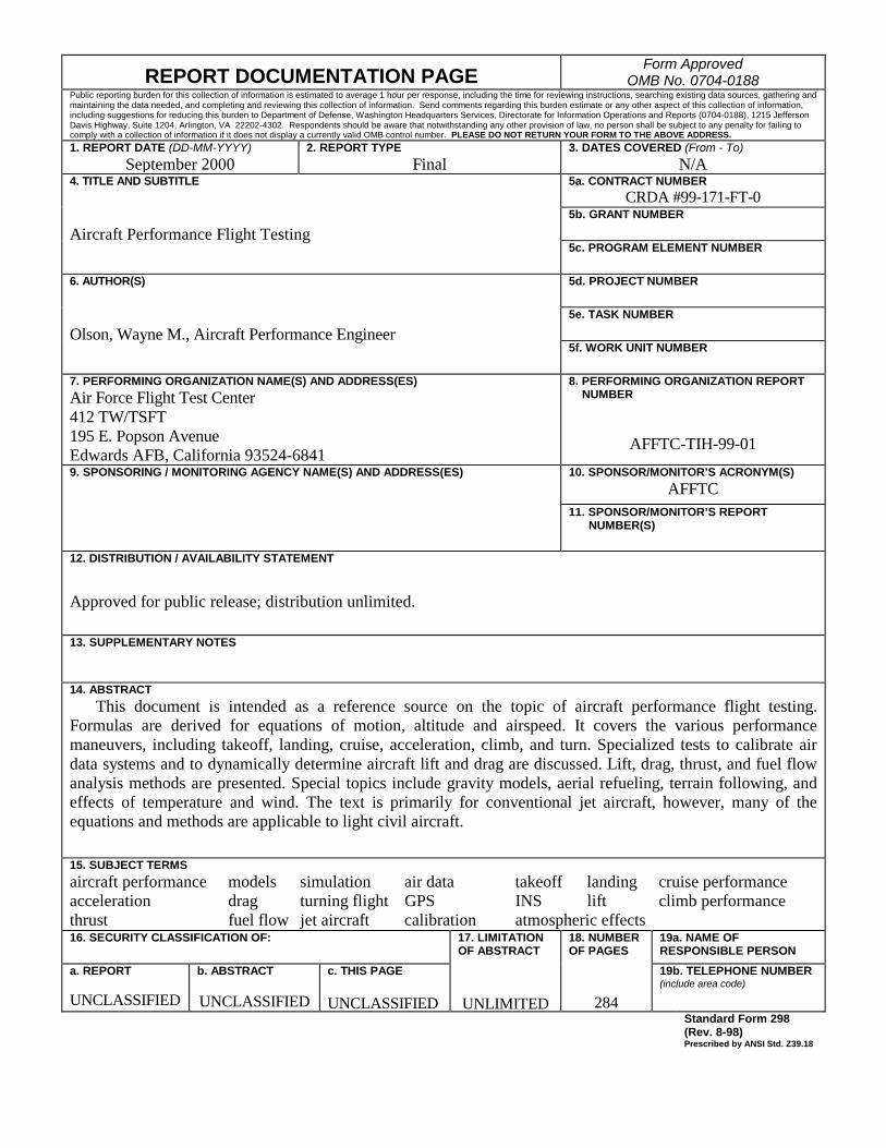
REPORT DOCUMENTATION PAGE Form Approved

OMB No. 0704-0188 Public reporting burden for this collection of information is estimated to average 1 hour per response, including the time for reviewing instructions, searching existing data sources, gathering and maintaining the data needed, and completing and reviewing this collection of information. Send comments regarding this burden estimate or any other aspect of this collection of information, including suggestions for reducing this burden to Department of Defense, Washington Headquarters Services, Directorate for Information Operations and Reports (0704-0188), 1215 Jefferson Davis Highway, Suite 1204, Arlington, VA 22202-4302. Respondents should be aware that notwithstanding any other provision of law, no person shall be subject to any penalty for failing to comply with a collection of information if it does not display a currently valid OMB control number. PLEASE DO NOT RETURN YOUR FORM TO THE ABOVE ADDRESS. 1. REPORT DATE (DD-MM-YYYY)

September 2000 2. REPORT TYPE

Final 3. DATES COVERED (From - To)

N/A 5a. CONTRACT NUMBER

CRDA #99-171-FT-0 5b. GRANT NUMBER

4. TITLE AND SUBTITLE Aircraft Performance Flight Testing

5c. PROGRAM ELEMENT NUMBER 5d. PROJECT NUMBER 5e. TASK NUMBER

6. AUTHOR(S) Olson, Wayne M., Aircraft Performance Engineer

5f. WORK UNIT NUMBER

7. PERFORMING ORGANIZATION NAME(S) AND ADDRESS(ES) Air Force Flight Test Center 412 TW/TSFT 195 E. Popson Avenue Edwards AFB, California 93524-6841

8. PERFORMING ORGANIZATION REPORT NUMBER

AFFTC-TIH-99-01

10. SPONSOR/MONITOR’S ACRONYM(S) AFFTC

9. SPONSORING / MONITORING AGENCY NAME(S) AND ADDRESS(ES)

11. SPONSOR/MONITOR’S REPORT NUMBER(S)

12. DISTRIBUTION / AVAILABILITY STATEMENT Approved for public release; distribution unlimited.

13. SUPPLEMENTARY NOTES

14. ABSTRACT This document is intended as a reference source on the topic of aircraft performance flight testing.

Formulas are derived for equations of motion, altitude and airspeed. It covers the various performance maneuvers, including takeoff, landing, cruise, acceleration, climb, and turn. Specialized tests to calibrate air data systems and to dynamically determine aircraft lift and drag are discussed. Lift, drag, thrust, and fuel flow analysis methods are presented. Special topics include gravity models, aerial refueling, terrain following, and effects of temperature and wind. The text is primarily for conventional jet aircraft, however, many of the equations and methods are applicable to light civil aircraft.

15. SUBJECT TERMS aircraft performance models simulation air data takeoff landing cruise performance acceleration drag turning flight GPS INS lift climb performance thrust fuel flow jet aircraft calibration atmospheric effects 16. SECURITY CLASSIFICATION OF:

17. LIMITATION OF ABSTRACT

18. NUMBER OF PAGES

19a. NAME OF RESPONSIBLE PERSON

a. REPORT

UNCLASSIFIED

b. ABSTRACT UNCLASSIFIED

c. THIS PAGE UNCLASSIFIED

UNLIMITED

284

19b. TELEPHONE NUMBER (include area code)

Standard Form 298 (Rev. 8-98) Prescribed by ANSI Std. Z39.18

iii

PREFACE

The author was employed at the Air Force Flight Test Center (AFFTC), Edwards AFB, California, from 1968 through 1993 as an aircraft performance flight test engineer. This document began, but was not finished, prior to his retirement in 1993. He endeavored to complete the document on his own and this text is the final result of that. He received a lot of help from the reviewers, which he mentions below they each made suggestions that improved the text vastly.

The intent of this text is that it should provide a highly useful reference source for aircraft performance flight test engineers. It certainly should not be the only source of information. The bibliography contains just a few of the sources that the author has found most useful. Much of the material covered in this handbook can be found in slightly different forms in the bibliographies listed in the Bibliography section. Even though the Flight Test Engineering Handbook (listed in the Bibliography Section) was originally written in the 1950s and updated slightly in the 1960s, it still contains much useful information. The author utilized Everett Dunlap’s Theory of the Measurement and Standardization of In-Flight Performance of Aircraft extensively as a reference source during his years at Edwards AFB. Also, the USAF Test Pilot School’s (TPS) Aircraft Performance manual was a valuable source, as well as the knowledge the author gained while a student at the USAF TPS.

The emphasis here is on performance testing as conducted at Edwards AFB; therefore, low budget or light aircraft testing is not covered extensively. Very little is said about instrumentation, except that it is needed and should be as accurate as reasonably possible. The thrust discussion is kept to a minimum. A number of other possible topics are discussed lightly, if not at all. Items not necessarily complete are:

1. airspeed calibration in ground effect,

2. test planning,

3. test conduct,

4. how to fly the maneuvers,

5. use of parameter identification,

6. report writing, and

7. cg accelerometer system.

This handbook is pieced together from writing the author has done going back as far as 1975. Much of it is from individual performance office memos which were written to stand-alone; therefore, you will see quite a bit of duplication. The same equation appears in several places the author tried to have the major derivation of the equation appear only once. For those of you who are familiar with the author’s style, you know he is big on theory and equations. Although it appears that there are a lot of intermediate steps in the derivations, the extra steps are appropriate to show where all the constants come from.

iv

Early versions of this text had three primary reviewers: Messrs. Mac McElroy, Ron Hart, and Frank Brown. Mr. McElroy looked at some early versions of this handbook. Messrs. Hart and Brown reviewed both the draft and final versions of this handbook. Mr. Bill Fish suggested adding the discussion of the ratio method of standardization and reviewed the thrust section. Mr. Allan Webb also reviewed the thrust section. Mr. Alan Lawless of the National TPS and Mr. John Hicks from NASA, Dryden Flight Research Center, provided significant comments that were implemented into the text. In addition, Mr. Richard Colgren of Lockheed-Martin Skunk Works and Captain Timothy Jorris of the AFFTC provided excellent suggestions that were incorporated.

There were many individual engineers at Edwards AFB that the author would like to acknowledge in this handbook. Although the list is long, they deserve mentioning. They are:

1. Mr. Jim Pape (who never found out the author did not know the difference between an aileron and an elevator when he first started working at Edwards AFB).

2. Mr. Willie Allen for teaching the author almost everything he knows about dynamic performance and flight path accelerometers. Mr. Allen invented the “cloverleaf” airspeed calibration method, which is discussed in this handbook.

3. Mr. Milton Porter for teaching the author the mathematics that he applied to the cloverleaf method in a mathematics class at the USAF TPS.

4. Mr. Randy Simpson of the Naval Air Test Center (now called the Naval Air Weapons Center). The author worked several months with Mr. Simpson on developing dynamic performance methods in the early 1970s.

5. Mr. Dave Richardson, while reviewing a very early version of this text, pointed out that the AFFTC and NASA were using dynamic performance methods on the lifting body research projects years before those of us in the conventional aircraft business.

6. Mr. Jim Olhausen of General Dynamics on the YF-16 and F-16A, who in the middle 1970s taught the author about using inertial navigation systems (INSs) for performance. As a result of Mr. Olhausen’s work, the INS became the primary source of flight path acceleration data on almost every large project at the AFFTC.

7. Mr. Al DeAnda for teaching the author about calibrating airspeed.

8. Mr. Bill Fish for tutoring the author in propulsion (though propulsion is discussed lightly in this handbook).

9. Mr. Bob Lee - The author worked with Mr. Lee for a short period of time in the early 1970s studying parameter identification.

10. Messrs. Clen Hendrickson, Lyle Schofield, Jim Cooper, Ken Rawlings, Mac McElroy, Ron Hart, Charlie Johnson, Pete Adolph, Don Johnson, Frank Brown and many others for helping the author learn about test techniques and other aspects of flight test.

Finally, the author would like to give sincere thanks to Mr. Frank Brown, his successor at Edwards AFB, for all his help in the preparation of this handbook. In addition, Ms. Virginia

v

O’Brien of Computer Sciences Corporation for the technical editing and final format of this handbook.

This will not be the final version of this handbook. The AFFTC would appreciate any suggestions for additional material, clarification of existing material, or any technical errors you may find. A form to submit proposed changes and/or improvements is included in the back of this handbook, or if needed, contact either Frank Brown or the author via e-mail with any comments. Following are addresses and e-mail for each of them.

Frank Brown 412 TW/TSFT Edwards, AFB, CA 93524-6841 [email protected] Wayne Olson 3003 NE 3rd Ave, #222 Camas, WA 98607-2340 [email protected] This March 2002 revision makes a few grammatical, spelling and formatting corrections. In

addition, a couple of equation numbers were misplaced. There have been no equation or other technical errors discovered so far.

This page intentionally left blank.

vi

TABLE OF CONTENTS

Page No.

PREFACE ...................................................................................................................................... iii

LIST OF ILLUSTRATIONS......................................................................................................... xi

LIST OF TABLES ......................................................................................................................... xvii

1.0 OVERVIEW ............................................................................................................................ 1 1.1 Introduction ....................................................................................................................... 1 1.2 Primary Instrumentation Parameters................................................................................. 1 1.3 Ground Tests ..................................................................................................................... 2 1.4 Flight Maneuvers............................................................................................................... 3 1.5 Data Analysis..................................................................................................................... 3

2.0 AXIS SYSTEMS AND EQUATIONS OF MOTION............................................................ 5 2.1 Flight Path Axis................................................................................................................. 5 2.2 Body Axis .......................................................................................................................... 7 2.3 True AOA and Sideslip Definitions ................................................................................. 8 2.4 In-Flight Forces ................................................................................................................. 10

SECTION 2.0 REFERENCE......................................................................................................... 12

3.0 ALTITUDE .............................................................................................................................. 13 3.1 Introduction – Altitude...................................................................................................... 13 3.2 Hydrostatic Equation......................................................................................................... 13 3.3 Geopotential Altitude........................................................................................................ 15 3.4 1976 U.S. Standard Atmosphere....................................................................................... 16 3.5 Temperature and Pressure Ratio....................................................................................... 16 3.6 Pressure Altitude ............................................................................................................... 18

3.6.1 Case 1: Constant Temperature ................................................................................18 3.6.2 Case 2: Linearly Varying Temperature ..................................................................19

3.7 Geopotential Altitude (H) versus Geometric Altitude (h) ............................................... 23 3.8 Geopotential versus Pressure Altitude - Nonstandard Day.............................................. 24 3.9 Effect of Wind Gradient.................................................................................................... 25 3.10 Density Altitude .............................................................................................................. 26 3.11 Pressure Altitude Error Due to Ambient Pressure Measurement Error......................... 28

4.0 AIRSPEED............................................................................................................................... 30 4.1 Introduction – Airspeed..................................................................................................... 30 4.2 Speed of Sound.................................................................................................................. 30 4.3 History of the Measurement of the Speed of Sound ........................................................ 31 4.4 The Nautical Mile ............................................................................................................. 32 4.5 True Airspeed.................................................................................................................... 32 4.6 Mach Number.................................................................................................................... 32 4.7 Total and Ambient Temperature....................................................................................... 35 4.8 Calibrated Airspeed........................................................................................................... 35 4.9 Equivalent Airspeed .......................................................................................................... 37 4.10 Mach Number from True Airspeed and Total Temperature.......................................... 37 4.11 Airspeed Error Due to Error in Total Pressure............................................................... 38

5.0 LIFT AND DRAG ................................................................................................................... 40 5.1 Introduction ....................................................................................................................... 40

vii

TABLE OF CONTENTS (Continued)

Page No.

5.2 Definition of Lift and Drag Coefficient Relationships .................................................... 40 5.3 The Drag Polar and Lift Curve ......................................................................................... 41 5.4 Reynolds Number.............................................................................................................. 42 5.5 Skin Friction Drag Relationships...................................................................................... 43 5.6 Idealized Drag Due to Lift Theories ................................................................................. 44 5.7 Air Force Flight Test Center Drag Model Formulation................................................... 45 5.8 The Terminology ‘Drag Polar’ ......................................................................................... 45

SECTION 5.0 REFERENCES ...................................................................................................... 48

6.0 THRUST .................................................................................................................................. 49 6.1 Introduction ....................................................................................................................... 49 6.2 The Thrust Equation.......................................................................................................... 50 6.3 In-Flight Thrust Deck........................................................................................................ 51 6.4 Status Deck........................................................................................................................ 51 6.5 Inlet Recovery Factor ........................................................................................................ 51 6.6 Thrust Runs ....................................................................................................................... 53 6.7 Thrust Dynamics ............................................................................................................... 54 6.8 Propeller Thrust................................................................................................................. 54

6.8.1 The Reciprocating Engine at Altitude .................................................................... 55

7.0 FLIGHT PATH ACCELERATIONS...................................................................................... 57 7.1 Airspeed-Altitude Method ................................................................................................ 57 7.2 GPS Method ...................................................................................................................... 58 7.3 Accelerometer Methods .................................................................................................... 58 7.4 Flight Path Accelerometer Method................................................................................... 58 7.5 Accelerometer Noise......................................................................................................... 60 7.6 Inertial Measurement Method........................................................................................... 66 7.7 Calculating Alpha, Beta and True Airspeed..................................................................... 66 7.8 Flight Path Accelerations .................................................................................................. 71 7.9 Accelerometer Rate Corrections....................................................................................... 72 7.10 Velocity Rate Corrections............................................................................................... 73 7.11 Calculating p, q, and r ..................................................................................................... 73 7.12 Euler Angle Diagram ...................................................................................................... 73

8.0 TAKEOFF................................................................................................................................ 74 8.1 General............................................................................................................................... 74 8.2 Takeoff Parameters ........................................................................................................... 74 8.3 Developing a Takeoff Simulation..................................................................................... 78 8.4 Ground Effect .................................................................................................................... 79 8.5 Effect of Runway Slope .................................................................................................... 87 8.6 Effect of Wind on Takeoff Distance................................................................................. 87 8.7 Takeoff Using Vectored Thrust ........................................................................................ 88 8.8 Effect of Thrust Component ............................................................................................. 92 8.9 Engine-Inoperative Takeoff .............................................................................................. 98 8.10 Idle Thrust Decelerations................................................................................................ 102

viii


Page No.

9.0 LANDING................................................................................................................................ 103 9.1 Braking Performance......................................................................................................... 103 9.2 Aerobraking....................................................................................................................... 106 9.3 Landing Air Phase............................................................................................................. 107 9.4 Landing on an Aircraft Carrier ......................................................................................... 109 9.5 Stopping Distance Comparison......................................................................................... 112 9.6 Takeoff and Landing Measurement.................................................................................. 113

10.0 AIR DATA SYSTEM CALIBRATION ............................................................................... 115 10.1 Historical Perspective...................................................................................................... 115 10.2 Groundspeed Course Method ......................................................................................... 115 10.3 General Concepts ............................................................................................................ 116 10.4 Pacer Aircraft .................................................................................................................. 119 10.5 Tower Flyby .................................................................................................................... 119 10.6 Accel-Decel ..................................................................................................................... 121 10.7 The Cloverleaf Method - Introduction............................................................................ 124 10.8 The Flight Maneuver....................................................................................................... 125 10.9 Error Analysis.................................................................................................................. 126 10.10 Air Force Flight Test Center Data Set .......................................................................... 126 10.11 Mathematics of the Cloverleaf Method........................................................................ 132

11.0 CRUISE.................................................................................................................................. 135 11.1 Introduction ..................................................................................................................... 135 11.2 Cruise Tests ..................................................................................................................... 136 11.3 Range ............................................................................................................................... 136 11.4 Computing Range from Range Factor ............................................................................ 139 11.5 Constant Altitude Method of Cruise Testing ................................................................. 141 11.6 Range Mission................................................................................................................. 141 11.7 Slow Accel-Decel............................................................................................................ 142 11.8 Effect of Wind on Range ................................................................................................ 142

12.0 ACCELERATION AND CLIMB ......................................................................................... 144 12.1 Acceleration..................................................................................................................... 144 12.2 Climb ............................................................................................................................... 145 12.3 Sawtooth Climbs ............................................................................................................. 146 12.4 Continuous Climbs.......................................................................................................... 148 12.5 Climb Parameters ............................................................................................................ 149 12.6 Acceleration Factor (AF) ................................................................................................ 149

12.6.1 Two Numerical Examples for AF.........................................................................150 12.7 Normal Load Factor During A Climb ............................................................................ 152 12.8 Descent ............................................................................................................................ 153 12.9 Deceleration..................................................................................................................... 154

SECTION 12.0 REFERENCES .................................................................................................... 154 13.0 TURNING.............................................................................................................................. 155

13.1 Introduction ..................................................................................................................... 155 13.2 Accelerating or Decelerating Turns................................................................................ 155

ix


Page No.

13.3 Thrust-Limited Turns...................................................................................................... 155 13.4 Stabilized Turns............................................................................................................... 156 13.5 Lift-Limited Turns........................................................................................................... 156 13.6 Turn Equations ................................................................................................................ 157

13.6.1 Normal Load Factor .............................................................................................. 157 13.6.2 Turn Radius ........................................................................................................... 159

13.7 Turn Rate ......................................................................................................................... 159 13.8 Winds Aloft ..................................................................................................................... 160

14.0 DYNAMIC PERFORMANCE.............................................................................................. 164 14.1 Introduction ..................................................................................................................... 164 14.2 Roller Coaster.................................................................................................................. 164 14.3 Windup Turn ................................................................................................................... 167 14.4 Split-S .............................................................................................................................. 167 14.5 Pullup............................................................................................................................... 170 14.6 Angle of Attack ............................................................................................................... 172 14.7 Vertical Wind .................................................................................................................. 172

15.0 SPECIAL PERFORMANCE TOPICS ................................................................................. 173 15.1 Effect of Gravity on Performance................................................................................... 173 15.2 Performance Degradation during Aerial Refueling ....................................................... 176 15.3 Performance Degradation during Terrain Following..................................................... 177 15.4 Uncertainty in Performance Measurements ................................................................... 178 15.5 Sample Uncertainty Analysis.......................................................................................... 178 15.6 Wind Direction Definition .............................................................................................. 179

16.0 STANDARDIZATION.......................................................................................................... 180 16.1 Introduction ..................................................................................................................... 180 16.2 Increment Method ........................................................................................................... 180

16.2.1 Climb/Descent ....................................................................................................... 181 16.2.2 Acceleration/Deceleration..................................................................................... 181 16.2.3 Accelerating/Decelerating Turn............................................................................ 182 16.2.4 Cruise..................................................................................................................... 182 16.2.5 Thrust-Limited Turn.............................................................................................. 182

16.3 Ratio Method................................................................................................................... 182

17.0 A SAMPLE PERFORMANCE MODEL ............................................................................. 184 17.1 Introduction ..................................................................................................................... 184 17.2 Drag Model...................................................................................................................... 184

17.2.1 Minimum Drag Coefficient................................................................................... 184 17.3 Skin Friction Drag Coefficient........................................................................................ 188 17.4 Drag Due to Lift .............................................................................................................. 189 17.5 Thrust and Fuel Flow Model .......................................................................................... 193 17.6 Thrust Specific Fuel Consumption ................................................................................. 193 17.7 Military Thrust ................................................................................................................ 195 17.8 Maximum Thrust............................................................................................................. 197 17.9 Cruise............................................................................................................................... 198 17.10 Range ............................................................................................................................. 199 17.11 Endurance...................................................................................................................... 203

x

TABLE OF CONTENTS (Concluded)

Page No.

17.12 Acceleration Performance............................................................................................. 203 17.13 Military Thrust Acceleration ........................................................................................ 204 17.14 Maximum Thrust Acceleration..................................................................................... 207 17.15 Sustained Turn............................................................................................................... 210

18.0 CRUISE FUEL FLOW MODELING ................................................................................... 213 18.1 Thrust Specific Fuel Consumption ................................................................................. 215 18.2 Multiple Regression ........................................................................................................ 216

SECTION 18.0 REFERENCE....................................................................................................... 219

19.0 EQUATIONS AND CONSTANTS...................................................................................... 220 19.1 Equations ......................................................................................................................... 220 19.2 Constants ......................................................................................................................... 229

APPENDIX A - AVERAGE WINDS AND TEMPERATURES FOR THE AIR FORCE FLIGHT TEST CENTER............................................................. 231

APPENDIX B - WEATHER TIME HISTORIES ........................................................................ 237

APPENDIX C - AVERAGE SURFACE WEATHER FOR THE AIR FORCE FLIGHT TEST CENTER............................................................. 241

BIBLIOGRAPHY .......................................................................................................................... 245

LIST OF ABBREVIATIONS, ACRONYMS, AND SYMBOLS ............................................... 249

INDEX............................................................................................................................................ 261 AIRCRAFT PERFORMANCE FLIGHT TESTING CHANGE FORM

xi

LIST OF ILLUSTRATIONS

xii

Figure No. Title Page No.

2.1 Aircraft Axis System................................................................................. 7

2.2 Angle of Attack and Sideslip Definitions................................................. 8

2.3 In-Flight Forces .........................................................................................10

2.4 Axis System Angle Diagram ....................................................................11

3.1 Element of Air...........................................................................................14

3.2 Logarithmic Variation of Pressure Ratio..................................................22

3.3 Standard Atmosphere Temperature..........................................................23

4.1 True Airspeed versus Calibrated Airspeed...............................................36

4.2 True Airspeed Error for 0.001 in. Hg Error .............................................38

5.1 Ratio of Compressible to Incompressible Dynamic Pressure..................41

5.2 Skin Friction Drag Relationships..............................................................44

5.3 Drag Polar..................................................................................................46

5.4 Lift-to-Drag Ratio versus Lift Coefficient................................................47

6.1 Turbine Engine Schematic........................................................................49

6.2 Normal Shock Recovery Factor................................................................52

6.3 F-15 Inlet Schematic .................................................................................53

6.4 Thrust Dynamics from an Air Force Flight Test Center Thrust Stand....54

7.1 Air Force Flight Test Center Nose Boom Instrumentation Unit .............60

7.2 Longitudinal Load Factor – Unfiltered Data............................................61

7.3 Normal Load Factor – Unfiltered Data ....................................................62

7.4 Four-Pole Butterworth Filter Attenuation Characteristics.......................63

7.5 Four-Pole Butterworth Filter Group Time Delay.....................................64

7.6 Longitudinal Load Factor – Filtered Data................................................65

7.7 Third-Order Polynomial Fit of Filtered Longitudinal Load Factor Data.................................................................65

7.8 Euler Angles..............................................................................................74

8.1 Takeoff and Landing Forces and Angles..................................................75

8.2 Predicted Ground Effect Drag ..................................................................80

8.3 Lift Ratio In-Ground Effect ......................................................................82

8.4 Takeoff Forces ..........................................................................................85

8.5 Takeoff Parameters ...................................................................................86

xiii

LIST OF ILLUSTRATIONS (Continued)


8.6 Effect of Wind........................................................................................... 88

8.7 F-16 Dimensions ....................................................................................... 89

8.8 Distance to Lift-Off................................................................................... 91

8.9 Angle of Attack at Lift-Off ....................................................................... 91

8.10 Effect of Thrust Component on Lift-Off Speed....................................... 92

8.11 Effect of Thrust Component on Distance to Lift-Off .............................. 93

8.12 Delta Tail Lift for Tail Area = 60 ft2 ........................................................ 94

8.13 Delta Tail Lift for Tail Area = 80 ft2 ........................................................ 95

8.14 Distance to Lift-Off versus Airspeed........................................................ 96

8.15 Calibrated Airspeed at Lift-Off ................................................................ 96

8.16 Takeoff Lift Model.................................................................................... 97

8.17 Takeoff Drag Model.................................................................................. 98

8.18 Takeoff Parameters versus Time .............................................................. 99

8.19 Takeoff Forces versus Airspeed ...............................................................100

8.20 Takeoff Forces versus Airspeed: Engine Inoperative .............................101

9.1 Braking Forces ..........................................................................................103

9.2 Stopping Distance versus Mu (µ )...........................................................104

9.3 Deceleration versus Calibrated Airspeed .................................................104

9.4 Mu versus Groundspeed (Wet Runway) ..................................................105

9.5 Braking Forces versus Calibrated Airspeed .............................................106

9.6 Total Resistance Force Comparison.........................................................107

9.7 Final Descent Rate versus Initial Descent Rate .......................................108

9.8 Landing Air Phase.....................................................................................109

9.9 F/A-18 with Tailhook Extended ...............................................................110

9.10 The U.S.S. Nimitz .....................................................................................110

10.1 Groundspeed Course – Heading Method .................................................115

10.2 Groundspeed Method – Direction Method ..............................................116

10.3 Flyby Tower Grid......................................................................................120

10.4 Altitude versus Grid Reading for Flyby Tower .......................................120

xiv



10.5 Effect of 10-Foot Error in Flyby Tower Altitude.....................................121

10.6 Pressure Survey.........................................................................................123

10.7 Accel-Decel Delta H .................................................................................123

10.8 Accel-Decel Position Error Coefficient....................................................124

10.9 Cloverleaf Flight Maneuver......................................................................126

10.10 Air Force Flight Test Center F-15 Pacer ..................................................126

10.11 Position Error ............................................................................................129

10.12 Groundspeed – Run 1a..............................................................................130

10.13 Groundspeed – Run 1b..............................................................................130

10.14 Groundspeed – Run 1c..............................................................................131

10.15 True Airspeed............................................................................................131

12.1 Specific Excess Power from Acceleration ...............................................145

12.2 AC-119G Aircraft .....................................................................................147

12.3 AC-119G Sawtooth Climb Data...............................................................147

12.4 AC-119G Excess Thrust Data ..................................................................148

12.5 Acceleration Factor – Constant Calibrated Airspeed...............................150

12.6 Acceleration Factor – Constant Mach Number........................................152

12.7 Centripetal Acceleration Diagram............................................................152

13.1 Normal Load Factor Vectors In a Turn ....................................................157

13.2 Banked Turn Diagram...............................................................................158

14.1 Drag Model ...............................................................................................165

14.2 Roller Coaster Normal Load Factor .........................................................166

14.3 Roller Coaster Altitude Time History ......................................................166

14.4 Roller Coaster Mach Number Time History............................................167

14.5 Split-S Drag Model ...................................................................................169

14.6 Split-S Normal Load Factor......................................................................169

14.7 Split-S Mach Number Time History ........................................................170

14.8 Split-S Altitude Time History...................................................................170

14.9 Pullup Mach Number Time History .........................................................171

xv



14.10 Pullup Altitude Time History ...................................................................171

17.1 Subsonic Drag Increment..........................................................................185

17.2 Transonic Drag Increment ........................................................................185

17.3 Supersonic Drag Increment.......................................................................186

17.4 Summary of Delta Drag Coefficient.........................................................188

17.5 Skin Friction Drag Coefficient .................................................................188

17.6 Drag Due to Lift Slope..............................................................................190

17.7 Drag Model at 0.8 Mach Number.............................................................191

17.8 Subsonic Drag Model ...............................................................................192

17.9 Drag Model – All Mach Numbers............................................................192

17.10 Thrust Specific Fuel Consumption...........................................................194

17.11 Military Referred Net Thrust ....................................................................196

17.12 Military Thrust ..........................................................................................196

17.13 Referred Net Thrust for Maximum Thrust...............................................197

17.14 Maximum Thrust.......................................................................................198

17.15 Range Factor .............................................................................................200

17.16 Maximum Range Factor ...........................................................................201

17.17 Range Factor – Altitude Effect .................................................................201

17.18 Range Factor – Variation with Temperature............................................202

17.19 Fuel Flow - Endurance..............................................................................203

17.20 Military Thrust Specific Excess Power ....................................................205

17.21 Military Thrust – Specific Excess Power, Temperature Effect ...............205

17.22 Military Thrust – Thrust and Drag at 10,000 Feet ...................................206

17.23 Drag at 10,000 Feet – Temperature Variation..........................................207

17.24 Maximum Thrust Specific Excess Power ................................................208

17.25 Maximum Thrust Specific Excess Power Temperature Effect at 30,000 Feet ................................................................................................208

17.26 Acceleration Time – Variation with Thrust .............................................210

17.27 Maximum Thrust – Sustained Turn Normal Load Factor .......................211

xvi

LIST OF ILLUSTRATIONS (Concluded)


18.1 C-17A Aircraft ..........................................................................................213

18.2 Thrust Specific Fuel Consumption...........................................................215

18.3 Percentage Error in Thrust Specific Fuel Consumption ..........................218

18.4 Range Factor Variation with Altitude ......................................................219

A1 Delta Temperature at 10,000 Feet ............................................................233





A6 Wind Direction..........................................................................................235

A7 Windspeed.................................................................................................236

A8 Geometric Height minus Pressure Altitude..............................................236

B1 Delta Temperature Time History..............................................................239

B2 Wind Direction Time History...................................................................240

B3 Windspeed Time History..........................................................................240

C1 Average Maximum and Minimum Surface Temperatures ......................243

xvii

LIST OF TABLES

Table No. Title Page No.

3.1 1976 U.S. Standard Atmosphere .............................................................. 17

3.2 Standard Atmosphere Pressure and Temperature .................................... 17

3.3 Edwards Average Weather Data for January ........................................... 25

3.4 Energy Altitude Effect of Wind Gradient ................................................ 26

3.5 Pressure Error Versus Altitude Error ....................................................... 29

5.1 Reynolds Number Variation with Mach Number and Altitude............... 42

7.1 Summary of Statistics for Longitudinal Load Factor............................... 66

8.1 Takeoff Events .......................................................................................... 86

8.2 Effect of Runway Slope ............................................................................ 87

8.3 Forces at Lift-Off Speed ........................................................................... 97

8.4 Takeoff Parameters at Flight Events ........................................................100

8.5 Takeoff Parameters at Significant Events-Engine-Inoperative................101

9.1 Ground Effect Parameters for F/A-18 Carrier Landing...........................111

9.2 Change in True Airspeed During Landing Due to Ground Effect...........112

9.3 Dry, Wet, and Aerobraking Data Summary .............................................113

9.4 Integration of Braking Results ..................................................................113

10.1 Aircraft Average Measurements and Parameters.....................................128

10.2 Inertial Speeds (GPS)................................................................................128

10.3 Outputs ......................................................................................................129

11.1 B-52G Cruise Data....................................................................................136

11.2 Range Factor Versus Altitude for B-52G.................................................140

12.1 Climb Ceiling Definitions.........................................................................146

14.1 Pullup and Split-S Initial and End Conditions .........................................172

15.1 Effect of Latitude on Gravity at Sea Level...............................................174

15.2 Effect of Altitude on Gravity....................................................................175

15.3 Effect of Heading and Speed on Normal Load Factor.............................175

15.4 Effect of Heading on Drag Coefficient ....................................................176

15.5 Parameter Uncertainties ............................................................................178

17.1 Tabulated Drag Rise Data.........................................................................187

17.2 Range Factor Variation with Altitude ......................................................202

17.3 Range Factor Variation with Temperature...............................................203

17.4 Drag Variation with Temperature.............................................................207

xviii


1

1.0 OVERVIEW

1.1 Introduction

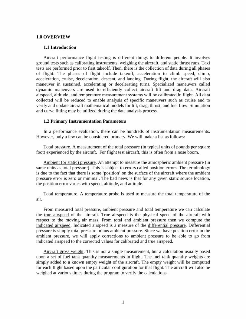
Aircraft performance flight testing is different things to different people. It involves ground tests such as calibrating instruments, weighing the aircraft, and static thrust runs. Taxi tests are performed prior to first takeoff. Then, there is the collection of data during all phases of flight. The phases of flight include takeoff, acceleration to climb speed, climb, acceleration, cruise, deceleration, descent, and landing. During flight, the aircraft will also maneuver in sustained, accelerating or decelerating turns. Specialized maneuvers called dynamic maneuvers are used to efficiently collect aircraft lift and drag data. Aircraft airspeed, altitude, and temperature measurement systems will be calibrated in flight. All data collected will be reduced to enable analysis of specific maneuvers such as cruise and to verify and update aircraft mathematical models for lift, drag, thrust, and fuel flow. Simulation and curve fitting may be utilized during the data analysis process.

1.2 Primary Instrumentation Parameters

In a performance evaluation, there can be hundreds of instrumentation measurements. However, only a few can be considered primary. We will make a list as follows:

Total pressure. A measurement of the total pressure (in typical units of pounds per square foot) experienced by the aircraft. For flight test aircraft, this is often from a nose boom.

Ambient (or static) pressure. An attempt to measure the atmospheric ambient pressure (in same units as total pressure). This is subject to errors called position errors. The terminology is due to the fact that there is some ‘position’ on the surface of the aircraft where the ambient pressure error is zero or minimal. The bad news is that for any given static source location, the position error varies with speed, altitude, and attitude.

Total temperature. A temperature probe is used to measure the total temperature of the air.

From measured total pressure, ambient pressure and total temperature we can calculate the true airspeed of the aircraft. True airspeed is the physical speed of the aircraft with respect to the moving air mass. From total and ambient pressure then we compute the indicated airspeed. Indicated airspeed is a measure of the differential pressure. Differential pressure is simply total pressure minus ambient pressure. Since we have position error in the ambient pressure, we will apply corrections to ambient pressure to be able to go from indicated airspeed to the corrected values for calibrated and true airspeed.

Aircraft gross weight. This is not a single measurement, but a calculation usually based upon a set of fuel tank quantity measurements in flight. The fuel tank quantity weights are simply added to a known empty weight of the aircraft. The empty weight will be computed for each flight based upon the particular configuration for that flight. The aircraft will also be weighed at various times during the program to verify the calculations.

2

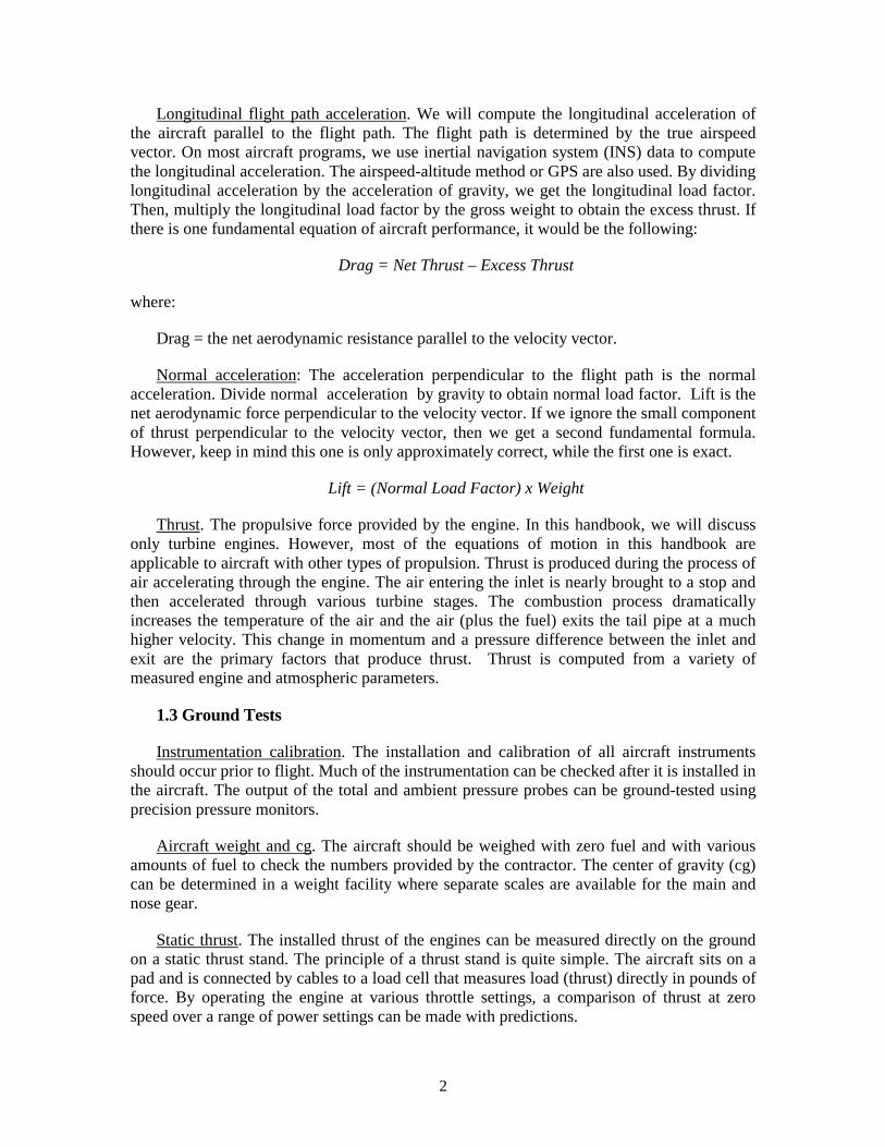
Longitudinal flight path acceleration. We will compute the longitudinal acceleration of the aircraft parallel to the flight path. The flight path is determined by the true airspeed vector. On most aircraft programs, we use inertial navigation system (INS) data to compute the longitudinal acceleration. The airspeed-altitude method or GPS are also used. By dividing longitudinal acceleration by the acceleration of gravity, we get the longitudinal load factor. Then, multiply the longitudinal load factor by the gross weight to obtain the excess thrust. If there is one fundamental equation of aircraft performance, it would be the following:

Drag = Net Thrust – Excess Thrust

where:

Drag = the net aerodynamic resistance parallel to the velocity vector.

Normal acceleration: The acceleration perpendicular to the flight path is the normal acceleration. Divide normal acceleration by gravity to obtain normal load factor. Lift is the net aerodynamic force perpendicular to the velocity vector. If we ignore the small component of thrust perpendicular to the velocity vector, then we get a second fundamental formula. However, keep in mind this one is only approximately correct, while the first one is exact.

Lift = (Normal Load Factor) x Weight

Thrust. The propulsive force provided by the engine. In this handbook, we will discuss only turbine engines. However, most of the equations of motion in this handbook are applicable to aircraft with other types of propulsion. Thrust is produced during the process of air accelerating through the engine. The air entering the inlet is nearly brought to a stop and then accelerated through various turbine stages. The combustion process dramatically increases the temperature of the air and the air (plus the fuel) exits the tail pipe at a much higher velocity. This change in momentum and a pressure difference between the inlet and exit are the primary factors that produce thrust. Thrust is computed from a variety of measured engine and atmospheric parameters.

1.3 Ground Tests

Instrumentation calibration. The installation and calibration of all aircraft instruments should occur prior to flight. Much of the instrumentation can be checked after it is installed in the aircraft. The output of the total and ambient pressure probes can be ground-tested using precision pressure monitors.

Aircraft weight and cg. The aircraft should be weighed with zero fuel and with various amounts of fuel to check the numbers provided by the contractor. The center of gravity (cg) can be determined in a weight facility where separate scales are available for the main and nose gear.

Static thrust. The installed thrust of the engines can be measured directly on the ground on a static thrust stand. The principle of a thrust stand is quite simple. The aircraft sits on a pad and is connected by cables to a load cell that measures load (thrust) directly in pounds of force. By operating the engine at various throttle settings, a comparison of thrust at zero speed over a range of power settings can be made with predictions.

3

Taxi tests. While taxiing on the ground, the aircraft is tested. Taxi means simply to move the aircraft under its own power on the ground without achieving flight. The first taxi tests would be accomplished in the lowest power setting called idle. The idle taxi tests, combined with the static thrust data, will quantify idle thrust at low speeds. Taxi tests at higher throttle settings and approaching lift-off speeds will give an early indication of thrust and drag on the ground. The final test, prior to first takeoff, will be to rotate the aircraft to lift-off attitude.

1.4 Flight Maneuvers

Takeoff tests are performed to determine the distance required to lift-off and to clear an obstacle. In USAF testing, the obstacle clearance height is 50 feet, while in civilian testing, the height is 35 feet for heavy aircraft and 50 feet for light aircraft. Lift-off is usually defined as when lift first becomes greater than weight. For multi-engine aircraft, engine-out testing is also performed wherein one engine’s power is reduced to idle to simulate an engine failure during takeoff.

Climb tests are flown to determine time, distance, and fuel used to climb to a cruise altitude. In addition, rate of climb versus altitude is determined.

Cruise testing is conducted to evaluate aircraft range. The aircraft is flown in stabilized flight over a range of speed and altitude conditions in order to determine the best speed and altitude to achieve maximum range. However, with modern analysis methods, the optimum range conditions are usually determined through analysis of drag and thrust/fuel flow models, which are verified and updated using cruise and other data.

Acceleration tests are conducted during level 1-g flight at fixed throttle settings. These tests are used in conjunction with climb tests to determine the optimum climb profiles. They are also used to update thrust and fuel flow models for fixed throttle settings over a range of altitudes and ambient temperature conditions. Excess thrust (thrust minus drag) is measured versus speed at various altitudes.

Turning performance is conducted to both determine ability of the aircraft to turn and to assist in generating aircraft lift and drag models at higher lift and angle-of-attack values than what are obtainable in 1-g flight.

Deceleration and descent tests are conducted to determine ability of the aircraft to decelerate and the fuel used in descent maneuvers. In addition, this data can be used to assist in generating aircraft thrust/fuel flow and drag models.

Landing tests are used to measure the distance to land starting from clearing an obstacle (as in the takeoff test). Braking tests performed during the landings or as separate tests, will evaluate stopping performance as well as the ability of the brakes to withstand the high temperatures associated with maximum performance braking.

1.5 Data Analysis

Thrust. Engine thrust is evaluated at fixed throttle settings. For military aircraft, these settings are usually designated IDLE, MIL (military) and MAX (maximum). Idle is the minimum throttle setting, MIL is the maximum throttle setting without the use of afterburner,

4

and MAX is the Maximum throttle setting with the use of afterburner. Thrust at these fixed throttle positions is primarily a function of flight conditions (speed, altitude, and temperature). A secondary function is angle of attack (angle between the aircraft body x-axis and the airspeed vector). Thrust is not measured directly, but rather computed from flight conditions and engine parameter measurements. The engine parameters needed usually include pressure, temperature, and rpm (revolutions per minute). Thrust is then computed using an engine manufacturer-provided computer program as modified by the airframe contractor to include installation effects. This is designated an in-flight thrust deck. A second computer program is usually provided a prediction deck, which will predict thrust without knowing any engine parameters (just flight conditions and throttle setting). The flight test data analyst will compare the in-flight thrust deck data to the prediction deck data. Then, analysis will be performed to attempt to ‘model’ this data.

Fuel flow. Engine fuel flow will be measured, modeled, and plotted versus thrust and as a function of flight conditions. Fuel flow data will be obtained both during the fixed throttle maneuvers (climb, accel, and turn) and during cruise testing. Fixed throttle refers to a specified throttle position like MIL, MAX or IDLE.

Lift. Lift in the form of a nondimensional lift coefficient will be determined and modeled versus angle of attack and Mach number.

Drag. Drag will be computed from thrust and excess thrust and modeled versus lift in nondimensional coefficient form.

5

2.0 AXIS SYSTEMS AND EQUATIONS OF MOTION

2.1 Flight Path Axis

The true airspeed vector defines the flight path (or wind) axis. The inertial velocity vector defines the inertial flight path axis. In this text, when the singular axis is used, we are usually referring to the longitudinal or x component of the wind axis system. The component of aerodynamic force parallel to the flight path axis is defined as drag. Lift is the component of aerodynamic force perpendicular to the drag (or flight path) axis. The component of aircraft acceleration parallel to the flight path is the longitudinal acceleration ( xA ). The longitudinal load factor ( xN ) is simply the xA divided by the acceleration of gravity ( g ). In conventional aircraft performance, g is assumed a constant at the reference gravity and given the value of 32.174 ft/sec² (foot per second squared). The symbol 0g will be used to denote the reference gravity. The effect of assuming a constant g is dealt with in the gravity section.

To derive the equations of motion we could start with the following energy relationship:

E KE PE= + (2.1)

where:

E = total energy (foot-pounds), KE = kinetic energy (foot-pounds), and PE = potential energy (foot-pounds).

Then, assuming zero wind:

2

00.5 t

tWKE Vg = ⋅ ⋅

(2.2)

0tW m g= ⋅ (2.3)

tPE W H= ⋅ (2.4)

where:

m = aircraft mass (slugs), [(pounds force)(seconds)2/(foot)], tW = aircraft gross weight (pounds),

H = geopotential altitude (feet), and tV = true airspeed (feet/sec).

Note: It is assumed that tapeline (or geometric) altitude ( h ) and geopotential altitudes ( H ) are identical. The small difference of these two altitude parameters is discussed in the altitude section.

6

Adding the potential and kinetic energy relationships (2.2) and (2.4) and dividing by tW yields the following:

( )2

0/ 2

tt

t t

PE KE VE W H gW W = + = + ⋅

(2.5)

The energy per unit weight ( / tE W ) is called energy altitude (or energy height) ( EH ).

( )2

02t

EVH H g= + ⋅ (2.6)

Taking the derivative with respect to time (and ignoring wind) yields:

0

/ t tE

V dVdH dt dH dt g dt = + ⋅

(2.7)

The derivative of EH with respect to time is called specific excess power and given the symbology of sP . The Cambridge Air and Space Dictionary (Reference 2.1) gives the following definition of specific excess power: “Thrust power available to an aircraft in excess of that required to fly at a particular constant height and speed, thus being usable for climbing, accelerating or turning.”

Equation 2.7 then becomes:

( )0

ts E t

VP H H Vg = = + ⋅

! ! ! (2.8)

Dividing by tV yields:

( ) ( ) ( )0s t E t t tP V H V H V V g= = +! ! ! (2.9)

Envision an accelerometer aligned perfectly with the longitudinal flight path axis and calibrated in units of g. The accelerometer would be sensitive to both aircraft change in velocity ( /tdV dt ) and a component of gravity ( ( )/ / tdH dt V ). Equation (2.9) then becomes:

0x t tN H V V g= +! ! (2.10)

In performance analysis, the axis system of interest is the flight path axis and not the body or earth axis, so the subscript f (f for flight path) is usually deleted on the flight path axis load factors. That is, we use xN rather than

fxN or even wxN (subscript w is for wind

axis). Other references may use other symbologies.

7

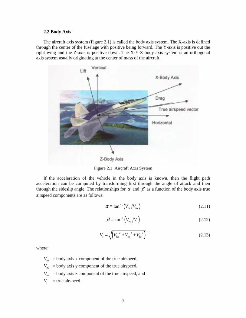
2.2 Body Axis

The aircraft axis system (Figure 2.1) is called the body axis system. The X-axis is defined through the center of the fuselage with positive being forward. The Y-axis is positive out the right wing and the Z-axis is positive down. The X-Y-Z body axis system is an orthogonal axis system usually originating at the center of mass of the aircraft.

Figure 2.1 Aircraft Axis System

If the acceleration of the vehicle in the body axis is known, then the flight path acceleration can be computed by transforming first through the angle of attack and then through the sideslip angle. The relationships for α and β as a function of the body axis true airspeed components are as follows:

( )1tan bz bxV Vα −= (2.11)

( )1sin by tV Vβ −= (2.12)

( )2 2 2t bx by bzV V V V= + + (2.13)

where:

bxV = body axis x component of the true airspeed,

byV = body axis y component of the true airspeed,

bzV = body axis z component of the true airspeed, and

tV = true airspeed.

8

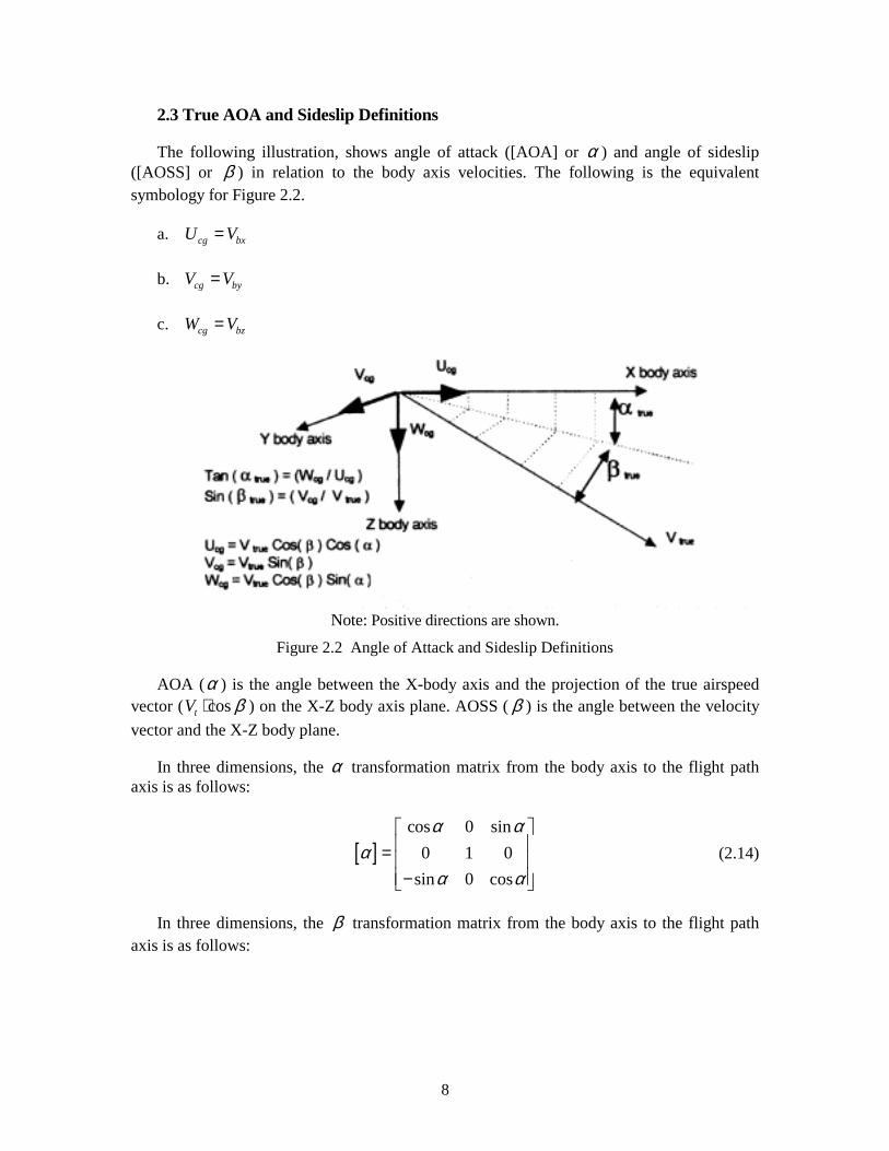
2.3 True AOA and Sideslip Definitions

The following illustration, shows angle of attack ([AOA] or α ) and angle of sideslip ([AOSS] or β ) in relation to the body axis velocities. The following is the equivalent symbology for Figure 2.2.

a. cg bxU V=

b. cg byV V=

c. cg bzW V=

Note: Positive directions are shown.

Figure 2.2 Angle of Attack and Sideslip Definitions

AOA (α ) is the angle between the X-body axis and the projection of the true airspeed vector ( costV β⋅ ) on the X-Z body axis plane. AOSS ( β ) is the angle between the velocity vector and the X-Z body plane.

In three dimensions, the α transformation matrix from the body axis to the flight path axis is as follows:

[ ]cos 0 sin

0 1 0sin 0 cos

α αα

α α

= −

(2.14)

In three dimensions, the β transformation matrix from the body axis to the flight path axis is as follows:

9

[ ]cos sin 0sin cos 00 0 1

β ββ β β

= −

(2.15)

The transformation of the acceleration from the body axis to the flight path axis is as follows (a subscript f [for flight path] will be dropped for the flight path axis):

cos sin 0 cos 0 sinsin cos 0 0 1 00 0 1 sin 0 cos

x bx

y by

z bz

A AA AA A

β β α αβ β

α α

= − ⋅ ⋅ −

(2.16)

Multiplying the equation 2.16 for the longitudinal load factor in the flight path axis yields equation 2.17.

cos cos sin cos sinx bx by bzA A A Aβ α β β α= ⋅ ⋅ + ⋅ + ⋅ ⋅ (2.17)

The vast majority of performance maneuvers produce very low sideslip and lateral acceleration such that equation 2.17 may be approximated by equation 2.18 assuming zero sideslip.

cos sinx bx bzA A Aα α≅ ⋅ + ⋅ (2.18)

In matrix shorthand, equation 2.16 is as follows:

{ } [ ] [ ] { }bA Aβ α= ⋅ (2.19)

where:

,,x y zA A A = three components of flight path accelerations, and

, ,bx by bzA A A = three components of body axis accelerations.

Usually, analysis is performed using the flight path axis load factors, as shown in equation 2.20 through 2.22, rather than the above flight path accelerations.

0/x xN A g= (2.20)

0/y yN A g= (2.21)

0/z zN A g= − (2.22)

Note the sign change on the Z component.

The topic of axis transformations is dealt with in more detail in the accelerometer section. There, we will deal with inertial axis (north, east, down), flight path axis, and with rate

10

corrections to accelerations and velocities in the body axis. Transformations are made to the body axis where the rate corrections are applied.

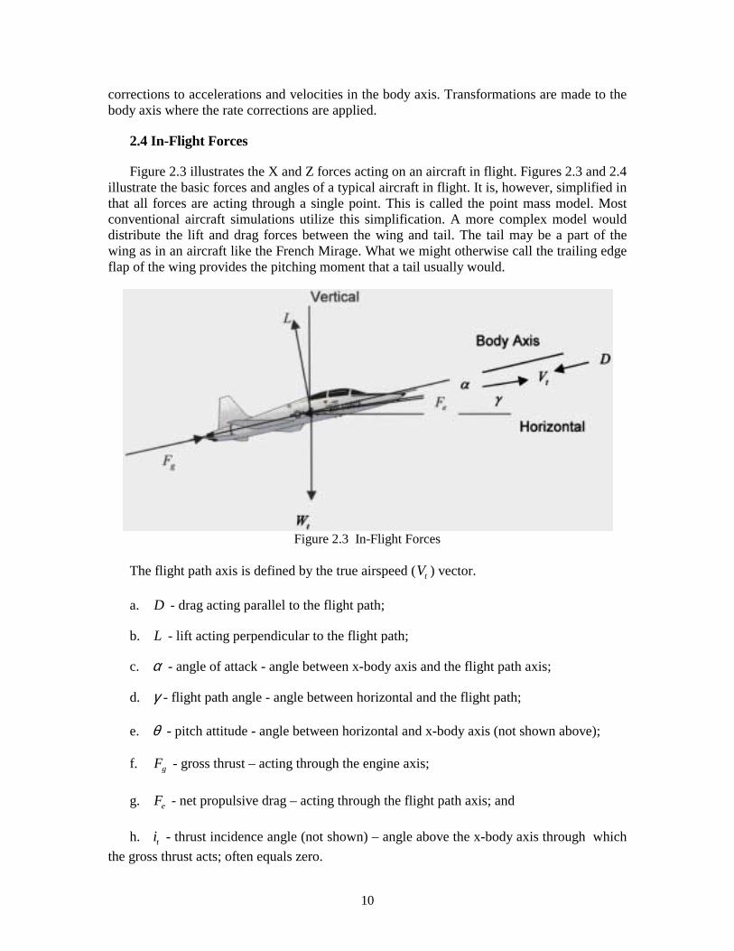
2.4 In-Flight Forces

Figure 2.3 illustrates the X and Z forces acting on an aircraft in flight. Figures 2.3 and 2.4 illustrate the basic forces and angles of a typical aircraft in flight. It is, however, simplified in that all forces are acting through a single point. This is called the point mass model. Most conventional aircraft simulations utilize this simplification. A more complex model would distribute the lift and drag forces between the wing and tail. The tail may be a part of the wing as in an aircraft like the French Mirage. What we might otherwise call the trailing edge flap of the wing provides the pitching moment that a tail usually would.

Figure 2.3 In-Flight Forces

The flight path axis is defined by the true airspeed ( tV ) vector.

a. D - drag acting parallel to the flight path;

b. L - lift acting perpendicular to the flight path;

c. α - angle of attack - angle between x-body axis and the flight path axis;

d. γ - flight path angle - angle between horizontal and the flight path;

e. θ - pitch attitude - angle between horizontal and x-body axis (not shown above);

f. gF - gross thrust – acting through the engine axis;

g. eF - net propulsive drag – acting through the flight path axis; and

h. ti - thrust incidence angle (not shown) – angle above the x-body axis through which the gross thrust acts; often equals zero.

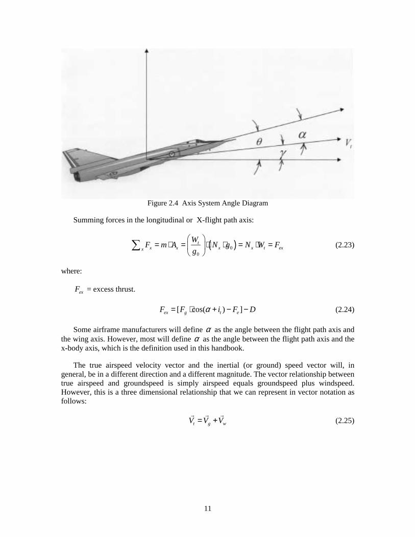
11

Figure 2.4 Axis System Angle Diagram

Summing forces in the longitudinal or X-flight path axis:

( )00

tx x x x t exx

WF m A N g N W Fg

= ⋅ = ⋅ ⋅ = ⋅ =

∑ (2.23)

where:

exF = excess thrust.

[ cos( ) ]ex g t eF F i F Dα= ⋅ + − − (2.24)

Some airframe manufacturers will define α as the angle between the flight path axis and the wing axis. However, most will define α as the angle between the flight path axis and the x-body axis, which is the definition used in this handbook.

The true airspeed velocity vector and the inertial (or ground) speed vector will, in general, be in a different direction and a different magnitude. The vector relationship between true airspeed and groundspeed is simply airspeed equals groundspeed plus windspeed. However, this is a three dimensional relationship that we can represent in vector notation as follows:

t g wV V V= +" " "

(2.25)

12

where:

true airspeed vectortV ="

,

ground speed vectorgV ="

, and

wind speed vectorwV ="

.

Wind direction, by meteorological convention, is the direction from which the wind is blowing. For instance, let’s say you are flying due north, with zero sideslip, at 500 knots. Heading is the direction the aircraft is pointing. Assume there is a 100 knot wind at 0 degrees. That would mean the wind is 100 knots blowing from due north. Or in this case, a pure headwind of 100 knots. If you have a 100-knot headwind and a 500-knot true airspeed then the groundspeed is 400 knots. Airspeed equals groundspeed plus wind (plus is italicized to place emphasis). There is, in the aero community, some controversy as to the sign convention. This author considers plus to be the ‘correct’ sign. However, if one uses a negative sign and is consistant with definitions, the results will come out the same.

Summing forces in the normal or Z-flight path axis:

( )00

tz z z z t

WF m A N g N Wg

= ⋅ = ⋅ ⋅ = ⋅

∑ (2.26)

sin( )z t g tN W L F iα⋅ = + ⋅ + (2.27)

where:

normal load factorzN = , and liftL = .

The propulsive drag ( eF ) is only in the longitudinal flight path axis so that its contribution normal to the flight path is zero.

SECTION 2.0 REFERENCE

2.1 Walker, P.M.B., ed. 1995. Cambridge Air and Space Dictionary. Cambridge University Press.

13

3.0 ALTITUDE

3.1 Introduction – Altitude

There are several forms of altitude of interest in aircraft performance. For this text, generally, all units will be in feet. The first altitude is geometric (or tapeline) altitude ( h ). Geometric altitude is the physical, linear altitude measured from mean sea level. Mean sea level is defined (from Britannica ) as the height of the sea surface averaged over all stages of the tide over a long period of time. The length of a foot of geometric altitude does not vary as a function of temperature or gravity variation with altitude. In the early days of flight, the technology was not available to measure altitude onboard an aircraft. However, they could measure the outside ambient pressure. A standard atmosphere was defined which allowed the computation of an altitude that was proportional to the ambient pressure. That altitude is the pressure altitude, which we will denote with the symbology CH , where c stands for calibrated. In order to derive a relationship between pressure and pressure altitude, it became necessary to define another altitude called geopotential altitude ( H ). The length of geopotential altitude foot varies with increasing altitude proportional to the change in gravity with altitude. The gravity model that has been used to define the geopotential altitude is a simplified model based upon reference gravity at sea level ( 0g = 32.174 ft/sec2) and gravity varying with altitude as per the inverse square gravity relationship.

For the standard atmosphere model, CH and H are identical by definition. This requires that sea level pressure is exactly the standard atmosphere value and that temperature is precisely standard day at all altitudes (not just at the altitude being considered). As will be shown later, the difference between h and H at 50,000 feet is less than 200 feet, but this difference grows in proportion the square of altitude from the center of earth, where the radius of the earth is over 20 million feet. Finally, an altitude commonly used to compute piston-powered light aircraft performance is density altitude ( dH ). Density altitude is useful for light aircraft primarily because engine performance is generally proportional more to density than to pressure for internal combustion engines. Density altitude is proportional to atmospheric density, just as pressure altitude is proportional to atmospheric pressure. Density altitude and pressure altitude is the same on a standard day at the altitude being considered. In this case, it is not required that temperatures be standard at all altitudes as was the case for H and Hc being identical.

3.2 Hydrostatic Equation

We will derive the relationship between atmospheric pressure and altitude. Envision a cubic element of air with unit horizontal dimensions ( dx and dy ) and a height equal to dh . The pressure on the bottom of the element is P . The pressure on the top of the element is P dP+ . The equation for static equilibrium of the element of air is as follows (the unit dimension into the page ( dy ) is not shown in Figure 3.1):

W g dx dy dzρ= ⋅ ⋅ ⋅ ⋅ =weight of the element of air (3.1)

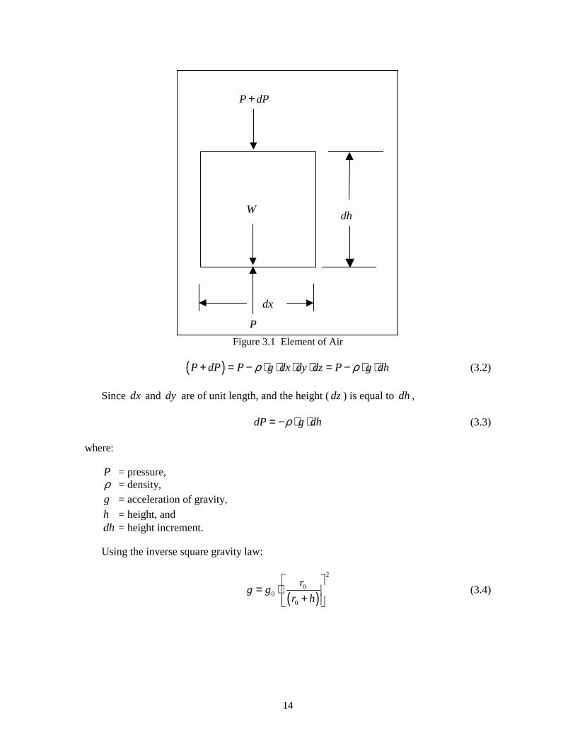
14

W

P dP+

P

dh

dx

Figure 3.1 Element of Air

( )P dP P g dx dy dz P g dhρ ρ+ = − ⋅ ⋅ ⋅ ⋅ = − ⋅ ⋅ (3.2)

Since dx and dy are of unit length, and the height ( dz ) is equal to dh ,

dP g dhρ= − ⋅ ⋅ (3.3)

where:

P = pressure, ρ = density, g = acceleration of gravity, h = height, and dh = height increment.

Using the inverse square gravity law:

( )

2

00

0

rg gr h

= ⋅ +

(3.4)

15

where:

0r = reference radius of the earth (20,855,553 ft), = 6,356,772 meters,

0g = reference gravity (32.17405 ft/sec²), and = 9.80665 m/sec2 (exactly by international agreement).

Introducing the ideal gas equation of state:

P R Tρ= ⋅ ⋅ (3.5)

Solving for ρ in 3.5:

( )P

R Tρ = ⋅ (3.6)

where:

T = ambient temperature, and R = gas constant = 3,089.8136 ft²/(sec²°K).

Value for R is converted from metric units using the 1976 U.S. Standard Atmosphere. Substituting 3.4 and 3.6 into 3.3:

2

00

0

rPdP g dhR T r h

= − ⋅ ⋅ ⋅ ⋅ + (3.7)

( ) ( ) ( ) 20 0 0/ 1/dP P g R T r r h dh = − ⋅ ⋅ + ⋅ (3.8)

It is not a simple matter to integrate the above equation exactly. The concept of a geopotential altitude was introduced to allow for the integration.

3.3 Geopotential Altitude

Geopotential altitude is developed from equation 3.9.

0g dh g dH⋅ = ⋅ (3.9)

where:

g = gravity at altitude h , h = tapeline (or geometric) altitude, and H = geopotential altitude.

16

A tapeline foot is the same physical length independent of height while a geopotential foot expands with increasing altitude linearly with the corresponding decrease in gravity.

0

gdH dhg

= ⋅

(3.10)

Substituting 3.10 into 3.3 and using 3.6:

( )0 0PdP g dH g dHR Tρ = − ⋅ ⋅ = − ⋅ ⋅ ⋅

(3.11)

( ) ( )0/ /dP P g R dH T= − ⋅ (3.12)

The above formula can be integrated if T either is a constant or is linearly varying with geopotential altitude ( H ). This means you can look up the integration formula in a table of integrals. A standard atmosphere model has been defined which contains only constant or linear temperature segments. The first standard atmosphere, defined by the French in 1919, contained just one segment. The constants in that segment are still the same today (as of 1976). This standard atmosphere purports to represent an average temperature model of the earth’s atmosphere throughout the world and during the various seasons.

3.4 1976 U.S. Standard Atmosphere

The 1976 U.S. Standard Atmosphere model is (as of the writing of this handbook) the accepted temperature and pressure profile model in the United States. The profile is presented in Tables 3.1 and 3.2. The region up to about 17 kilometers (56,000 feet) is known as the troposphere. Quoting from Britannica Online: “troposphere - a term derived from the Greek words tropos, ‘turning’ and sphaira, ‘ball’.” The temperature decreases rapidly with altitude in this region. The rising warm air meets the sinking cold air and the air tends to “turn over” like a “ball” – hence the term troposphere. One would pause between layers, hence, the transition to the next layer is called the tropopause. To about 50 kilometers (164,000 feet), the temperature rises slowly in a region called the stratosphere. Altitudes higher than 50 kilometers are above the region of conventional aircraft performance, so we will not discuss those. However, the temperatures for the model atmosphere are included in Tables 3.1 and 3.2 to a geometric altitude of 86 kilometers.

3.5 Temperature and Pressure Ratio

We will define temperature ratio (θ ) and pressure ratio (δ ). These are, respectively, the ratio of ambient temperature to standard temperature at sea level and the ratio of ambient pressure to standard pressure at sea level. The formulas are as follows:

288.15SL

T TT

θ = = (3.13)

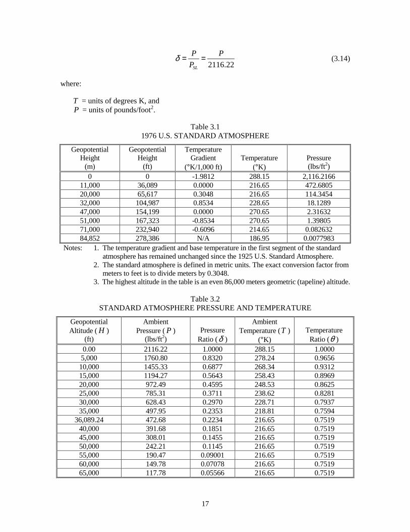
17

2116.22SL

P PP

δ = = (3.14)

where:

T = units of degrees K, and P = units of pounds/foot2.

Table 3.1 1976 U.S. STANDARD ATMOSPHERE

Geopotential Height

(m)

Geopotential Height

(ft)

Temperature Gradient

(°K/1,000 ft)

Temperature

(°K)

Pressure (lbs/ft2)

0 0 -1.9812 288.15 2,116.2166 11,000 36,089 0.0000 216.65 472.6805 20,000 65,617 0.3048 216.65 114.3454 32,000 104,987 0.8534 228.65 18.1289 47,000 154,199 0.0000 270.65 2.31632 51,000 167,323 -0.8534 270.65 1.39805 71,000 232,940 -0.6096 214.65 0.082632 84,852 278,386 N/A 186.95 0.0077983

Notes: 1. The temperature gradient and base temperature in the first segment of the standard atmosphere has remained unchanged since the 1925 U.S. Standard Atmosphere.

2. The standard atmosphere is defined in metric units. The exact conversion factor from meters to feet is to divide meters by 0.3048.

3. The highest altitude in the table is an even 86,000 meters geometric (tapeline) altitude.

Table 3.2 STANDARD ATMOSPHERE PRESSURE AND TEMPERATURE

Geopotential Altitude ( H )

(ft)

Ambient Pressure ( P )

(lbs/ft2)

Pressure

Ratio (δ )

Ambient Temperature (T )

(°K)

Temperature

Ratio (θ ) 0.00 2116.22 1.0000 288.15 1.0000

5,000 1760.80 0.8320 278.24 0.9656 10,000 1455.33 0.6877 268.34 0.9312 15,000 1194.27 0.5643 258.43 0.8969 20,000 972.49 0.4595 248.53 0.8625 25,000 785.31 0.3711 238.62 0.8281 30,000 628.43 0.2970 228.71 0.7937 35,000 497.95 0.2353 218.81 0.7594

36,089.24 472.68 0.2234 216.65 0.7519 40,000 391.68 0.1851 216.65 0.7519 45,000 308.01 0.1455 216.65 0.7519 50,000 242.21 0.1145 216.65 0.7519 55,000 190.47 0.09001 216.65 0.7519 60,000 149.78 0.07078 216.65 0.7519 65,000 117.78 0.05566 216.65 0.7519

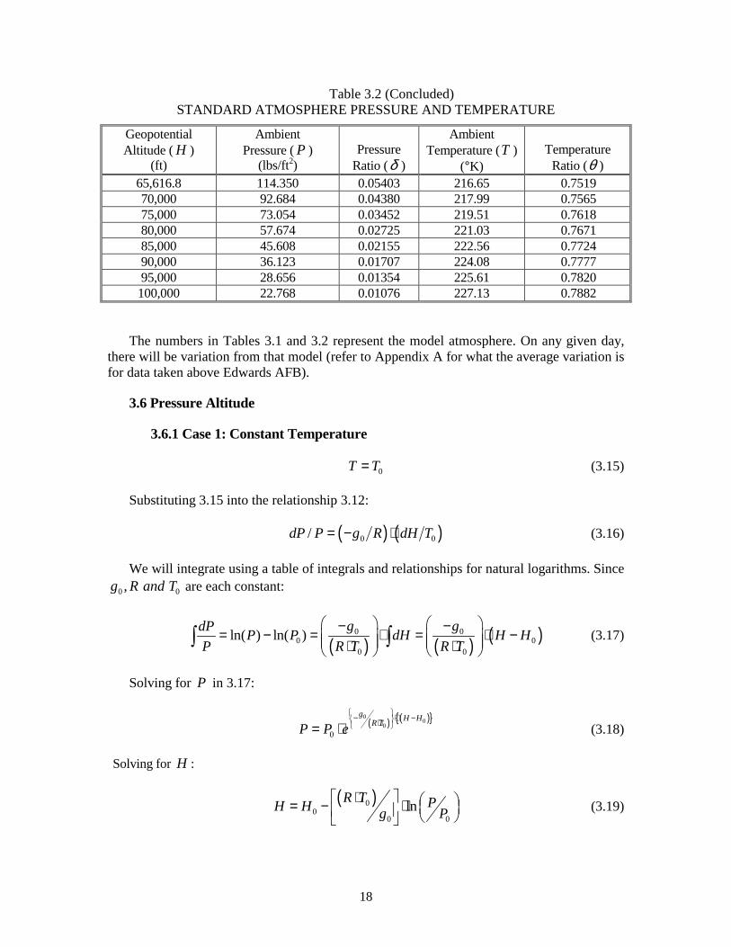
18

Table 3.2 (Concluded) STANDARD ATMOSPHERE PRESSURE AND TEMPERATURE

Geopotential Altitude ( H )

(ft)

Ambient Pressure ( P )

(lbs/ft2)

Pressure

Ratio (δ )

Ambient Temperature (T )

(°K)

Temperature

Ratio (θ ) 65,616.8 114.350 0.05403 216.65 0.7519 70,000 92.684 0.04380 217.99 0.7565 75,000 73.054 0.03452 219.51 0.7618 80,000 57.674 0.02725 221.03 0.7671 85,000 45.608 0.02155 222.56 0.7724 90,000 36.123 0.01707 224.08 0.7777 95,000 28.656 0.01354 225.61 0.7820

100,000 22.768 0.01076 227.13 0.7882

The numbers in Tables 3.1 and 3.2 represent the model atmosphere. On any given day, there will be variation from that model (refer to Appendix A for what the average variation is for data taken above Edwards AFB).

3.6 Pressure Altitude

3.6.1 Case 1: Constant Temperature

0T T= (3.15)

Substituting 3.15 into the relationship 3.12:

( ) ( )0 0/dP P g R dH T= − ⋅ (3.16)

We will integrate using a table of integrals and relationships for natural logarithms. Since 0 0,g R and T are each constant:

( ) ( ) ( )0 0

0 00 0

ln( ) ln( ) g gdP P P dH H HP R T R T

− −= − = ⋅ = ⋅ − ⋅ ⋅ ∫ ∫ (3.17)

Solving for P in 3.17:

( ) ( ){ }00

00

g H HR TP P e − ⋅ − ⋅ = ⋅ (3.18)

Solving for H :

( )00

0 0lnR T PH H g P

⋅ = − ⋅ (3.19)

19

For the segment of the atmosphere from 11,000 meters (36,089 feet) to 20,000 meters (65,617 feet):

a. 0T = 216.65 °K (-69.7 °F or -56.5 °C),

b. 0P = 472.68 pounds/ft2 0at H H= , and

c. 0H = 36,089.24 feet (11,000 m).

3.6.2 Case 2: Linearly Varying Temperature

Assume a temperature that varies linearly with altitude as follows:

( )0 0T T a H H= + ⋅ − (3.20)

where:

0T = base temperature,

0H = base geopotential altitude, and a = temperature gradient (deg K/foot). Substituting, again, into the relationship (3.12) ( ) ( )0/ /dP P g R dH T= − ⋅ :

[ ]( )0

0 0

/ gdP P dHR T a H H

= − ⋅ ⋅ + ⋅ −

(3.21)

Integrating from a table of integrals:

( ) ( )1 lndx a bxa b x b

= ⋅ ++ ⋅∫

Then using the relationship ln( ) ln( ) ln( / )u v u v− = :

( )( )( )0 00

0 0

ln lnT a H HgP

P R a T

+ − = − ⋅ ⋅ (3.22)

Solving for P :

( )( )

0

0 00

1g

R aaP P H HT

− ⋅ = ⋅ + ⋅ − (3.23)

Or solving for H :

20

( )

00

00

1R a

g TPH H P a

− ⋅ = + − ⋅

(3.24)

For the first segment of the standard atmosphere (zero to 11,000 meters; zero to 36,089.24 feet), substituting constants (from the international standard atmosphere) [for English units]:

( )0

1.9812 /10006.8755856 6

288.15a ET− = = − (round to 6.87559 6E − ) (3.25)

( ) ( )0 32.17405 5.255876

3089.8136 1.9812 /1000g

R a− = =⋅ ⋅ (round to 5.2559) (3.26)

( )5.2559

01 6.87559 6P E HP = − − ⋅ (3.27)

Solving for H :

( )

( )

1 5.2559

01

6.87559 6

PP

HE

− =−

(3.28)

Equation 3.26 is the definition of pressure altitude for altitudes from zero to 36,089 feet (zero to 11,000 meters).

Using the pressure ratio (δ) as defined in equation 3.14.

SL

PPδ = (3.29)

where:

SLP = standard sea level pressure = 101,325 pascals (exactly, by international agreement).

The unit pascal has been defined as a newton of force per square meter. A newton has units of (kg m/sec2). One newton is equal to 0.2248195 pounds force.

In various English units:

SLP = 2,116.2166 pounds/ft² (usually rounded to 2,116.22);

≅ 760 mm Hg;

= 1,013.25 millibar (mb); and

= 29.92 in. Hg

21

Substituting 3.29 into 3.28:

( )

( )

1 5.25591

6.87559 6CHE

δ − =−

(3.30)

The above is for zero to 36,089 feet pressure altitude.

The symbol CH is used for pressure altitude to distinguish it from the geopotential altitude ( H ). Pressure altitude and geopotential altitudes are only identical for the model atmosphere.

Similarly:

( )5.25591 6.87559 6 CE Hδ = − − ⋅ (3.31)

For the temperature ratio (θ ), using equation 3.20 and substituting constants (from the international standard atmosphere):

0 1.9812 1 6.87559 6288.15 288.15 1,000

TT H E Hθ = = − ⋅ = − − ⋅ (3.32)

The second segment of the standard atmosphere (11,000 to 20,000 meters) (36,089 to 65,617 feet) is a constant temperature (T =-56.5 degrees C) segment. The standard atmosphere is defined in metric units. English units require the conversion factor of 0.3048 meters per foot. For instance, the 11,000-meter point is 36,089.24 feet.

For the altitude segment between 36,089 feet and 65,617 feet:

( )0 0

32.17405/( ) 4.806343 53089.8136 216.65

g R T E⋅ = = −⋅

(3.33)

0

020,805.84R T

g⋅ =

Computing δ for 36,089.24H = feet using the δ formula for the first segment of the atmosphere (equation 3.31):

[ ] ( ){ }4.806343 5 36089.240.22336 CE Heδ − − ⋅ −= ⋅ (3.34)

For the temperature ratio (θ ), using equation 3.20 and substituting constants (from the international standard atmosphere):

0 1.9812 1 6.87559 6288.15 288.15 1,000

TT H E Hθ = = − ⋅ = − − ⋅ (3.35)

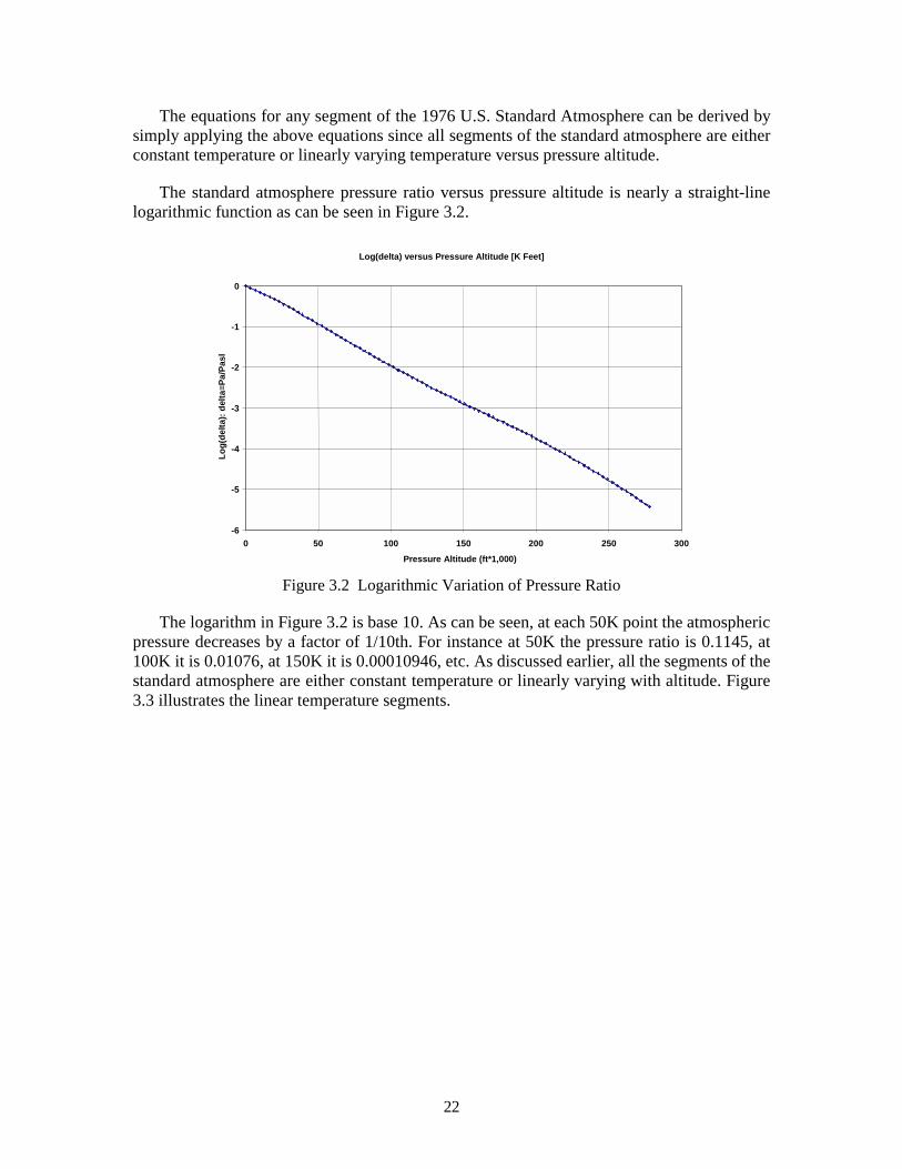
22

The equations for any segment of the 1976 U.S. Standard Atmosphere can be derived by simply applying the above equations since all segments of the standard atmosphere are either constant temperature or linearly varying temperature versus pressure altitude.

The standard atmosphere pressure ratio versus pressure altitude is nearly a straight-line logarithmic function as can be seen in Figure 3.2.

Log(delta) versus Pressure Altitude [K Feet]

-6

-5

-4

-3

-2

-1

0

0 50 100 150 200 250 300

Pressure Altitude (ft*1,000)

Log(

delta

): de

lta=P

a/Pa

sl

Figure 3.2 Logarithmic Variation of Pressure Ratio

The logarithm in Figure 3.2 is base 10. As can be seen, at each 50K point the atmospheric pressure decreases by a factor of 1/10th. For instance at 50K the pressure ratio is 0.1145, at 100K it is 0.01076, at 150K it is 0.00010946, etc. As discussed earlier, all the segments of the standard atmosphere are either constant temperature or linearly varying with altitude. Figure 3.3 illustrates the linear temperature segments.

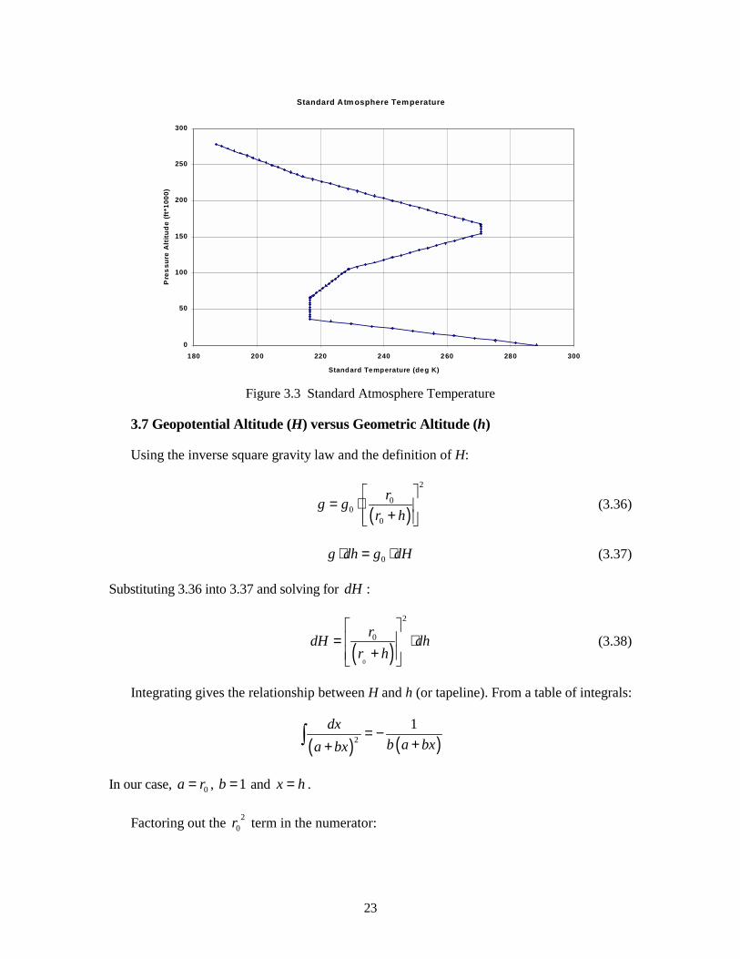
23

Standard Atm osphere Temperature

0

50

100

150

200

250

300

180 200 220 240 260 280 300

Standard Temperature (deg K)

Pre

ssur

e A

ltitu

de

(ft*

1000

)

Figure 3.3 Standard Atmosphere Temperature

3.7 Geopotential Altitude (H) versus Geometric Altitude (h)

Using the inverse square gravity law and the definition of H:

( )

2

00

0

rg gr h

= ⋅ +

(3.36)

0g dh g dH⋅ = ⋅ (3.37)

Substituting 3.36 into 3.37 and solving for dH :

( )0

2

0rdH dhr h

= ⋅

+ (3.38)

Integrating gives the relationship between H and h (or tapeline). From a table of integrals:

( ) ( )2

1dxb a bxa bx

= −++∫

In our case, 0a r= , 1b = and x h= .

Factoring out the 20r term in the numerator:

24

( ) ( )

2 20 02

0 00 0

1 1h dhH r rr h rr h

= ⋅ = ⋅ − + ++

∫ (3.39)

Multiply the first term in square brackets by 0

0

rr and the second term by ( )

( )0

0

r hr h

++ .

( )

( )( )

2 000

0 0 0 0

r hrH rr h r r h r

+−= ⋅ + + ⋅ + ⋅ (3.40)

By factoring terms, we get:

( )

0

0

rH hr h

= ⋅ +

[ ]0 20,855,553 feetr = (3.41)

At 50,000 feet tapeline altitude (the upper limit of most conventional aircraft performance testing), H computes to be 49,881 feet, for a difference of only 119 feet, or 0.24 percent.

3.8 Geopotential versus Pressure Altitude - Nonstandard Day

A standard temperature may exist at a given altitude on a test day but there would never be a standard atmosphere at all altitudes except in computer models.

Using the basic /dP P relationship (3.12):

0( / ) ( / )C STDdP P g R dH T= − ⋅ standard day (3.42)

0( / ) ( / )dP P g R dH T= − ⋅ test day (3.43)

There can be a significant difference between having a standard atmosphere and achieving standard temperature at a given altitude. The pressure levels at a given pressure altitude are by definition the same whatever the temperature. Therefore, we could equate the right sides of equations 3.42 and 3.43.

/ /C STDdH T dH T= (3.44)

where:

test dayT T= .

CSTD

TdH dHT = ⋅

(3.45)

Since dh dH≅ (i.e., ∆ tapeline ≅ ∆ geopotential):

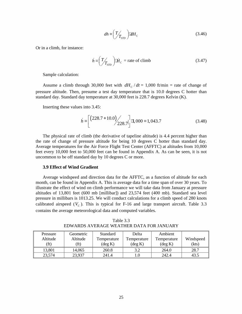
25

CSTD

Tdh dHT = ⋅

(3.46)

Or in a climb, for instance:

CSTD

Th HT = ⋅

! ! = rate of climb (3.47)

Sample calculation:

Assume a climb through 30,000 feet with /CdH dt = 1,000 ft/min = rate of change of pressure altitude. Then, presume a test day temperature that is 10.0 degrees C hotter than standard day. Standard day temperature at 30,000 feet is 228.7 degrees Kelvin (K).

Inserting these values into 3.45:

( )228.7 10.0 1,000 1,043.7228.7h += ⋅ =

! (3.48)

The physical rate of climb (the derivative of tapeline altitude) is 4.4 percent higher than the rate of change of pressure altitude for being 10 degrees C hotter than standard day. Average temperatures for the Air Force Flight Test Center (AFFTC) at altitudes from 10,000 feet every 10,000 feet to 50,000 feet can be found in Appendix A. As can be seen, it is not uncommon to be off standard day by 10 degrees C or more.

3.9 Effect of Wind Gradient

Average windspeed and direction data for the AFFTC, as a function of altitude for each month, can be found in Appendix A. This is average data for a time span of over 30 years. To illustrate the effect of wind on climb performance we will take data from January at pressure altitudes of 13,801 feet (600 mb [millibar]) and 23,574 feet (400 mb). Standard sea level pressure in millibars is 1013.25. We will conduct calculations for a climb speed of 280 knots calibrated airspeed ( CV ). This is typical for F-16 and large transport aircraft. Table 3.3 contains the average meteorological data and computed variables.

Table 3.3 EDWARDS AVERAGE WEATHER DATA FOR JANUARY

Pressure Altitude

(ft)

Geometric Altitude

(ft)

Standard Temperature

(deg K)

Delta Temperature

(deg K)

Ambient Temperature

(deg K)

Windspeed

(kts) 13,801 14,065 260.8 3.2 264.0 28.7 23,574 23,937 241.4 1.0 242.4 43.5

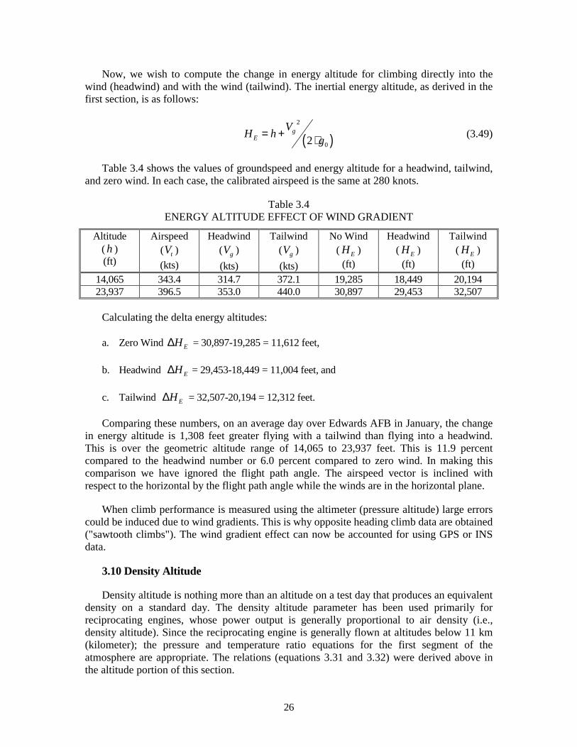
26

Now, we wish to compute the change in energy altitude for climbing directly into the wind (headwind) and with the wind (tailwind). The inertial energy altitude, as derived in the first section, is as follows:

( )2

02g

EVH h g= + ⋅ (3.49)

Table 3.4 shows the values of groundspeed and energy altitude for a headwind, tailwind, and zero wind. In each case, the calibrated airspeed is the same at 280 knots.

Table 3.4 ENERGY ALTITUDE EFFECT OF WIND GRADIENT

Altitude ( h ) (ft)

Airspeed

( tV ) (kts)

Headwind

( gV ) (kts)

Tailwind

( gV ) (kts)

No Wind

( EH ) (ft)

Headwind

( EH ) (ft)

Tailwind ( EH )

(ft) 14,065 343.4 314.7 372.1 19,285 18,449 20,194 23,937 396.5 353.0 440.0 30,897 29,453 32,507

Calculating the delta energy altitudes:

a. Zero Wind EH∆ = 30,897-19,285 = 11,612 feet,

b. Headwind EH∆ = 29,453-18,449 = 11,004 feet, and

c. Tailwind EH∆ = 32,507-20,194 = 12,312 feet.

Comparing these numbers, on an average day over Edwards AFB in January, the change in energy altitude is 1,308 feet greater flying with a tailwind than flying into a headwind. This is over the geometric altitude range of 14,065 to 23,937 feet. This is 11.9 percent compared to the headwind number or 6.0 percent compared to zero wind. In making this comparison we have ignored the flight path angle. The airspeed vector is inclined with respect to the horizontal by the flight path angle while the winds are in the horizontal plane.

When climb performance is measured using the altimeter (pressure altitude) large errors could be induced due to wind gradients. This is why opposite heading climb data are obtained ("sawtooth climbs"). The wind gradient effect can now be accounted for using GPS or INS data.

3.10 Density Altitude

Density altitude is nothing more than an altitude on a test day that produces an equivalent density on a standard day. The density altitude parameter has been used primarily for reciprocating engines, whose power output is generally proportional to air density (i.e., density altitude). Since the reciprocating engine is generally flown at altitudes below 11 km (kilometer); the pressure and temperature ratio equations for the first segment of the atmosphere are appropriate. The relations (equations 3.31 and 3.32) were derived above in the altitude portion of this section.

27

( )5.25591 6.87559 6 CE Hδ = − − ⋅

( )1 6.87559 6 CE Hθ = − − ⋅

The first formula (δ ) is valid for standard or any nonstandard day. That is, pressure ratio is a function of pressure altitude only and vice versa. On the other hand, the temperature ratio (θ ) formula is valid only for standard temperatures.

We can compute density ratio (σ ) for a standard day, by taking the ratio of the above formulas.

( )( ) ( )

5.25594.25591 6.87559 6

1 6.87559 61 6.87559 6

CC

C

E HE H

E Hδσθ

− − ⋅= = = − − ⋅

− − ⋅ (3.50)

The above σ formula is valid only for standard day. However, one could define the density altitude ( dH ) as being directly proportional to density as defined by equation 3.50.

( )4.25591 6.87559 6 dE Hσ = − − ⋅

Let’s give an example. We are at 10,000 feet pressure altitude at 100 degrees F. The pressure ratio is:

5.2559(1 6.87559 6 10,000) 0.6877Eδ = − − ⋅ =

On a standard day, the temperature would have been:

( )1 6.87559 6 10,000 0.9312Eθ = − − ⋅ = ( )288.15 288.15 0.9312 268.3 268.3 273.15 1.8 32 23.3T Fθ= ⋅ = ⋅ = = − ⋅ + = °

The standard day σ is:

0.6877 0.73840.9312

σ = =

Solving for dH

[ ] ( )[ ]1 4.25591 4.2559 11

6.87559 6 6.87559 6dHE E

δσ θ − − = =

− −

(3.51)

For the test day temperature of 100 degrees F:

28

( )459.67 1001.0790

518.67θ

+= =

The σ for the test day would be:

0.6877 0.63731.0790

δσθ

= = =

Then, computing dH we get:

1/ 4.25590.68771 / 6.87559 6

1.0790dH E = − −

(3.52)

14,607dH = feet versus 10,000 feet for CH (pressure altitude).

Equation 3.52 shows the density (or σ ) at 100 degrees F at 10,000 feet pressure altitude is the same as at 14,607 feet pressure altitude on a standard day for that altitude. To check on our calculations, calculate the standard density ratio for 14,607 feet as follows:

a. ( )5.25591 6.87559 6 14,607 0.5733Eδ = − − ⋅ = ,

b. (1 6.87559 6 14,607) 0.8996Eθ = − − ⋅ = , and

c. 0.5733 0.63730.8996

δσθ

= = = .

It checks! The density ratio for 100 degrees F at 10,000 feet pressure altitude is identical to the density ratio at a density altitude of 14,607 feet.

3.11 Pressure Altitude Error Due to Ambient Pressure Measurement Error

At Edwards AFB, the field elevation (geometric height) of the main runway (22/04) is 2,300 feet. With standard atmospheric conditions, the pressure altitude would also be 2,300 feet. That requires more than just being at standard temperature. As we have derived, pressure altitude is only a function of ambient pressure and is independent of ambient temperature. Using the standard atmosphere model formulas, we can compute what a 1-foot change in altitude will produce in ambient pressure. Table 3.5 shows the resultant pressure error for a 1-foot error in pressure altitude.

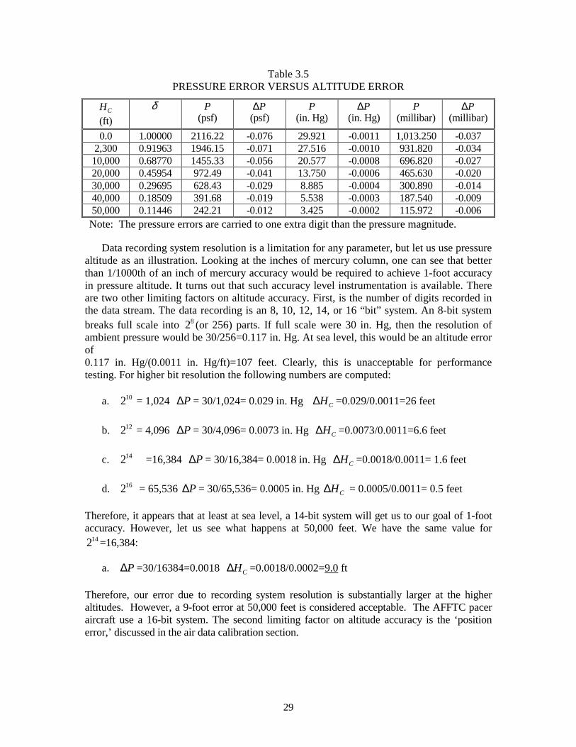
29

Table 3.5 PRESSURE ERROR VERSUS ALTITUDE ERROR

CH (ft)

δ P (psf)

P∆ (psf)

P (in. Hg)

P∆ (in. Hg)

P (millibar)

P∆ (millibar)

0.0 1.00000 2116.22 -0.076 29.921 -0.0011 1,013.250 -0.037 2,300 0.91963 1946.15 -0.071 27.516 -0.0010 931.820 -0.034 10,000 0.68770 1455.33 -0.056 20.577 -0.0008 696.820 -0.027 20,000 0.45954 972.49 -0.041 13.750 -0.0006 465.630 -0.020 30,000 0.29695 628.43 -0.029 8.885 -0.0004 300.890 -0.014 40,000 0.18509 391.68 -0.019 5.538 -0.0003 187.540 -0.009 50,000 0.11446 242.21 -0.012 3.425 -0.0002 115.972 -0.006

Note: The pressure errors are carried to one extra digit than the pressure magnitude.

Data recording system resolution is a limitation for any parameter, but let us use pressure altitude as an illustration. Looking at the inches of mercury column, one can see that better than 1/1000th of an inch of mercury accuracy would be required to achieve 1-foot accuracy in pressure altitude. It turns out that such accuracy level instrumentation is available. There are two other limiting factors on altitude accuracy. First, is the number of digits recorded in the data stream. The data recording is an 8, 10, 12, 14, or 16 “bit” system. An 8-bit system breaks full scale into 82 (or 256) parts. If full scale were 30 in. Hg, then the resolution of ambient pressure would be 30/256=0.117 in. Hg. At sea level, this would be an altitude error of 0.117 in. Hg/(0.0011 in. Hg/ft)=107 feet. Clearly, this is unacceptable for performance testing. For higher bit resolution the following numbers are computed:

a. 102 = 1,024 P∆ = 30/1,024= 0.029 in. Hg CH∆ =0.029/0.0011=26 feet

b. 122 = 4,096 P∆ = 30/4,096= 0.0073 in. Hg CH∆ =0.0073/0.0011=6.6 feet

c. 142 =16,384 P∆ = 30/16,384= 0.0018 in. Hg CH∆ =0.0018/0.0011= 1.6 feet

d. 162 = 65,536 P∆ = 30/65,536= 0.0005 in. Hg CH∆ = 0.0005/0.0011= 0.5 feet

Therefore, it appears that at least at sea level, a 14-bit system will get us to our goal of 1-foot accuracy. However, let us see what happens at 50,000 feet. We have the same value for

142 =16,384:

a. P∆ =30/16384=0.0018 CH∆ =0.0018/0.0002=9.0 ft

Therefore, our error due to recording system resolution is substantially larger at the higher altitudes. However, a 9-foot error at 50,000 feet is considered acceptable. The AFFTC pacer aircraft use a 16-bit system. The second limiting factor on altitude accuracy is the ‘position error,’ discussed in the air data calibration section.

30

4.0 AIRSPEED

4.1 Introduction – Airspeed

Aircraft speed can be expressed in several forms. For this text, generally, the units will be in either knots (nautical miles per hour) or feet per second, except for Mach number ( M ), which is dimensionless. Groundspeed ( gV ) is the physical speed relative to the ground and is usually expressed as a vector relationship with north, east, and down components. This is due to obtaining groundspeed from INS (inertial navigation system) or GPS (global positioning system) data sources. True airspeed ( tV ) is the physical speed of the aircraft with respect to the moving air mass. This is usually a scalar quantity, though components of true airspeed can be computed using axis transformations using INS velocities and angles and windspeeds. Windspeed ( wV ) is the speed of the air mass (wind) with respect to the ground. This is also a vector quantity with north, east and down components. The Mach number ( M ) is the ratio of true airspeed to the local speed of sound. Mach numbers less than 1 are referred to as subsonic and those greater than 1 are supersonic. The speed of sound is a function of the square root of the ambient temperature. Calibrated airspeed ( CV ) is the speed displayed on a typical cockpit airspeed indicator. It is a function of only one parameter differential (or impact) pressure. Impact pressure is the difference between total and ambient pressure. The c (calibrated) has two meanings. The first is that calibrated airspeed is ‘calibrated’ to sea level in the sense that it will be exactly equal to true airspeed at sea level, standard day, but only at that condition. The second is calibrated versus indicated. A pneumatic instrument (physically driven from pressure inputs) displays an ‘indicated’ value. The value has instrument and position errors. The instrument errors are errors due to the instrument itself. Position errors are those due to the location of pressure probes. There may be some ideal location to place probes where the errors are zero. However, in the real world, there is no such position so there will always be position errors of some magnitude. Once instrument and position error corrections are applied, the indicated airspeed becomes calibrated airspeed.

In aircraft equipped with an ADC (air data computer), those corrections are usually already applied in the ADC so that the displayed airspeed is calibrated airspeed. Calibrated airspeed, as mentioned above, is a function only of the impact pressure. That pressure is also designated compressible dynamic pressure. A measure of airspeed that is a function of incompressible dynamic pressure is called equivalent airspeed ( eV ). Structural analysis is often in terms of incompressible dynamic pressure, so that equivalent airspeed is a useful speed for structural testing. At sea level, standard day, calibrated airspeed and equivalent airspeed are equal (or equivalent), but only at that condition.

4.2 Speed of Sound

The speed of sound is computed by the following formula:

( )a R Tγ= ⋅ ⋅ (4.1)

31

where:

a = speed of sound (ft/sec), γ = 1.40 (ratio of specific heats), and R = 3,089.8136 ft²/(sec² °K) (from the 1976 U.S. Standard Atmosphere).

For a sea level standard day, T = 288.15 °K. Then,

[ ]1.40 3089.8136 288.15a = ⋅ ⋅ (4.2)

= 1,116.4505 ft/sec (usually rounded to 1116.45)

= 661.4788 knots (usually rounded to 661.48)

For the speed of sound at temperatures other than standard sea level,

( )

SL SLSL

R Ta Ta TR T

γγ

⋅ ⋅= =

⋅ ⋅ (4.3)

Then, define θ as the ratio of test day temperature to standard day temperature at sea level.

SLa a θ= ⋅ (4.4)

4.3 History of the Measurement of the Speed of Sound

From Britannica On-line, the speed of sound in air was first measured by the French scientist Pierre Gassendi in the 1600s at 478.4 meters per second. He “measured the time difference between spotting the flash of a gun and hearing its report over a long distance.” Very clever! In the 1650s, two Italians (Giovanni Borelli and Vincenzo Viviani) obtained a much more accurate value of 350 meters per second. The first precise value was obtained at the Academy of Sciences in Paris in 1738 at 332 meters per second. Britannica reports a value of 331.45 meters per second was obtained in 1942, which was amended to 331.29 meters per second in 1986. These values were at 0 degrees C.

In 1942, NACA (National Advisory Committee for Aeronautics) published Report No. 1235. In that report, they specified the speed of sound at sea level standard day as 1116.89 feet/second. Converting the NACA number to meters per second and to 0 degrees C:

a. 273.151116.89 0.3048 331.45288.15

a = ⋅ ⋅ = meters/second

In 1962 and again in 1976, the ICAO (International Civil Aviation Organization) agreed upon constants for use in a standard atmosphere. The speed of sound is not directly defined, but could be computed from the other constants. The speed of sound at sea level in English and metric units is as follows:

a. 1116.4505SLa = ft/sec = 340.2941 m/sec

32

4.4 The Nautical Mile

The nautical mile (nm) has been set, by international agreement, to exactly 1,852 meters. The conversion factor from feet to meters is also an exact number 0.3048 meters per foot. Therefore, we can compute the number of feet per nautical mile.

a. 1,852 / 0.3048 6,076.1155 feetNM = =

Since a knot is 1 nm per hour, the conversion from knots to feet per second is as follows:

a. 6,076.115 Hourfeet/sec 1.6878 knotsHour 3,600 sec

NM= ⋅ =

An early definition of a nautical mile was an even 6,080 feet. It is called the British nautical mile. With that definition, the conversion factor becomes:

a. 6,080. Hourfeet/sec 1.6889 knotsHour 3,600 sec

NM= ⋅ =

One would see the above conversion factor in textbooks published prior to the U.S. standard atmosphere of 1959, which had many of the same constants as the 1962 and 1976 atmospheres. Using the 1942 speed of sound and the early knots to feet per second conversion one gets:

a. 1,116.89 /1.6889 661.31 knotsSLa = =

With the modern (as of this writing) values:

b. 1,116.45 /1.6878 661.48 knotsSLa = =

4.5 True Airspeed

True airspeed ( tV ) is the physical speed of the vehicle relative to the moving air mass. The true airspeed is a vector quantity. The relationship between true airspeed and the speed with respect to the ground ( gV ) is:

t g wV V V= +" " "

= true airspeed vector (4.5)

where:

wV ="

windspeed vector.

4.6 Mach Number

Mach number ( M ) is defined as the ratio of true airspeed to the local speed of sound.

tVM a= (4.6)

33

We could compute Mach number from Pitot-static theory with the simple expression for

differential pressure ( Cq ) versus total pressure detected by a Pitot tube ( tP′ ) and ambient pressure ( P ). The prime on the total pressure is to denote a measurement behind a normal shock (for M ≥1). For M <1, the free stream total pressure ( tP ) and the measured total

pressure ( tP′ ) are identical. Differential pressure is also compressible dynamic pressure and often designated impact pressure.

Cq = tP′ − P

Or dividing both sides by P :

CqP =

tP′ P − 1 (4.8)

Using Bernoulli’s Equation for 1M < :

( ) ( )1211 12

Cq MP

γ γγ

− −= + ⋅ −

(4.9)

And the Rayleigh Supersonic Pitot Equation for 1M ≥ :

( ) ( ) ( )( ) ( )

( )1/ 11

21 12

11 12 1 2Cq MP M

γγ γ

γ

γγ

γ γ

− −

−

+ + = ⋅ ⋅ − − + ⋅ ⋅

(4.10)

Substituting γ =1.40 for M <1:

( )3.521 0.2 1cq MP = + ⋅ − (4.11)

Solving for M in equation 4.11:

[ ]1 3.5

5 1 1CqM P = ⋅ + −

(4.12)

For 1M ≥ :

( ) ( )

2.53.52

2

2.41.2 10.4 2.8

Cq MP M

= ⋅ ⋅ − − + ⋅

(4.13)

34

Multiply by 1= (2.50/2.50)2.5 and collect terms. Multiply the first term { 2 3.5(1.2 )M⋅ } by 2.52.50 and divide the second term in the { } brackets by the same 2.52.50 factor.

( )( ) ( )2.5

2 3.53.5 2.52.52

2.41.2 2.5 10.4 2.5 2.8 2.5

Cq MP M⋅= ⋅ ⋅ ⋅ −

− ⋅ + ⋅ ⋅ (4.14)

( )

73.5 2.5 2.5

2.521.2 2.5 2.4 1

7 1

M

M= ⋅ ⋅ ⋅ −

⋅ − (4.15)

3.5 2.5 2.51.2 2.5 2.4 166.9215801⋅ ⋅ = (round to 166.9216)

( )

72.52

166.9216 17 1

Cq MP M

= ⋅ − ⋅ −

(4.16)

Note that one produces the identical value for /Cq P when M = 1.0 is inserted into either the subsonic (equation 4.11) or supersonic (equation 4.16) formula. For example:

a. 1.0

/ 0.892929C Mq P

==

Solving for M in the supersonic formula (4.16), first add 1 to both sides, then multiply

both sides by the term ( )2.527 1M⋅ − .

( )2.52 71 7 1 166.9216Cq M MP + ⋅ ⋅ − = ⋅

Then, divide both sides by ( )2.527 M⋅ .

( )( ) [ ]

2.5 722

2 2 2.52.5

166.92167 11 1.2875607 7

CMMq MP M M ⋅

⋅ ⋅ − + ⋅ = = ⋅ ⋅ ⋅

Finally, solve for M from the M on the right side.

2.5

2

10.881285 1 17

CqM P M

= ⋅ + ⋅ − ⋅

(4.17)

As can be seen, M appears on both sides of the equation. One method to approach the supersonic M calculation in a computer algorithm is first determine if M is indeed greater than 1.0 by calculating M from the subsonic equation (4.12). If M is greater than 1.0 at that point, then use the value of M from the subsonic equation as the initial condition in the

35

supersonic equation. Then perform a simple iteration until M converges to a value - usually in just a few iterations.

4.7 Total and Ambient Temperature

A total temperature probe is used to measure total temperature ( tT ). Assuming this probe is in the freestream with no heat loss (adiabatic), then the relationship between total temperature and ambient temperature (T ) is as follows:

( ) ( )2 211 1 0.2

2tT T M T Mγ −

= ⋅ + ⋅ = ⋅ + ⋅

(4.18)

4.8 Calibrated Airspeed

Historically, airspeed indicators were constructed with a single pressure input being the differential pressure ( Cq ). The gauge is “calibrated” to read true airspeed at sea level standard pressure and temperature. The subsonic and supersonic Mach number equations are used with the simple substitutions of ( /C SLV a ) for M and SLP for P . However, the condition for which the equations are used is no longer subsonic ( M <1) or supersonic ( M >1) but rather calibrated airspeed being less or greater than the speed of sound ( SLa ), standard day, sea level (661.48 knots).

For C SLV a< :

3.52

1 0.2 1C C

SL SL

q VP a

= + ⋅ − (4.19)

(1 3.5)

5 1 1CC SL

SL

qV a P = ⋅ ⋅ + −

(4.20)

For C SLV a≥ :

( )

( )

7

2.52

166.92161

7 1

C SLC

SLC SL

V aqP

V a

⋅= − ⋅ −

(4.21)

Solving for CV and noting that the formula is similar in form to the M equation, we will leave out intermediate steps.

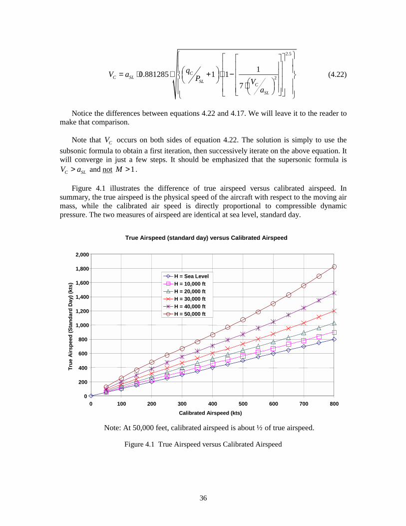
36

2.5

210.881285 1 1

7

CC SL

SLC

SL

qV a P Va

= ⋅ ⋅ + ⋅ − ⋅

(4.22)

Notice the differences between equations 4.22 and 4.17. We will leave it to the reader to make that comparison.

Note that CV occurs on both sides of equation 4.22. The solution is simply to use the subsonic formula to obtain a first iteration, then successively iterate on the above equation. It will converge in just a few steps. It should be emphasized that the supersonic formula is

C SLV a> and not 1M > .

Figure 4.1 illustrates the difference of true airspeed versus calibrated airspeed. In summary, the true airspeed is the physical speed of the aircraft with respect to the moving air mass, while the calibrated air speed is directly proportional to compressible dynamic pressure. The two measures of airspeed are identical at sea level, standard day.

True Airspeed (standard day) versus Calibrated Airspeed

0

200

400

600

800

1,000

1,200

1,400

1,600

1,800

2,000

0 100 200 300 400 500 600 700 800Calibrated Airspeed (kts)

True

Airs

peed

(Sta

ndar

d D

ay) (

kts)

H = Sea LevelH = 10,000 ftH = 20,000 ftH = 30,000 ftH = 40,000 ftH = 50,000 ft

Note: At 50,000 feet, calibrated airspeed is about ½ of true airspeed.

Figure 4.1 True Airspeed versus Calibrated Airspeed

37

4.9 Equivalent Airspeed

Equivalent airspeed is defined from the incompressible dynamic pressure formula.

2 200.5 0.5t eq V Vρ ρ= ⋅ ⋅ = ⋅ ⋅ (4.23)

0 ;SLSL

ρρ ρ σ ρ= = (4.24)

2 2e tV Vσ= ⋅ (4.25)

e tV Vσ= ⋅ (4.26)

For the performance engineer, there is no practical reason to use equivalent airspeed for anything. However, structural analysis is often performed in terms of equivalent airspeed (since it is a direct function of the incompressible dynamic pressure), so the performance engineer needs to be able to convert eV to parameters that are more useful. Besides equation 4.26, another useful equation is derived. Since Mach number is

( )t t

SL

V VM a a θ= =

⋅ (4.27)

And δσ θ= , then

( ) ( )e t SLV V a Mδσ θθ= ⋅ = ⋅ ⋅

( )e

SL

VMa δ

=⋅

(4.28)

Therefore, the equation 4.28 is a handy conversion between eV and M . Notice that it is not a function of temperature.

4.10 Mach Number from True Airspeed and Total Temperature

If one has an accurate direct measure of tV , then M can be computed with the additional measurement of total temperature ( tT ). The direct tV measure could come from laser velocimetry. For example:

288.15t SL

TV a M

= ⋅ ⋅

(4.29)

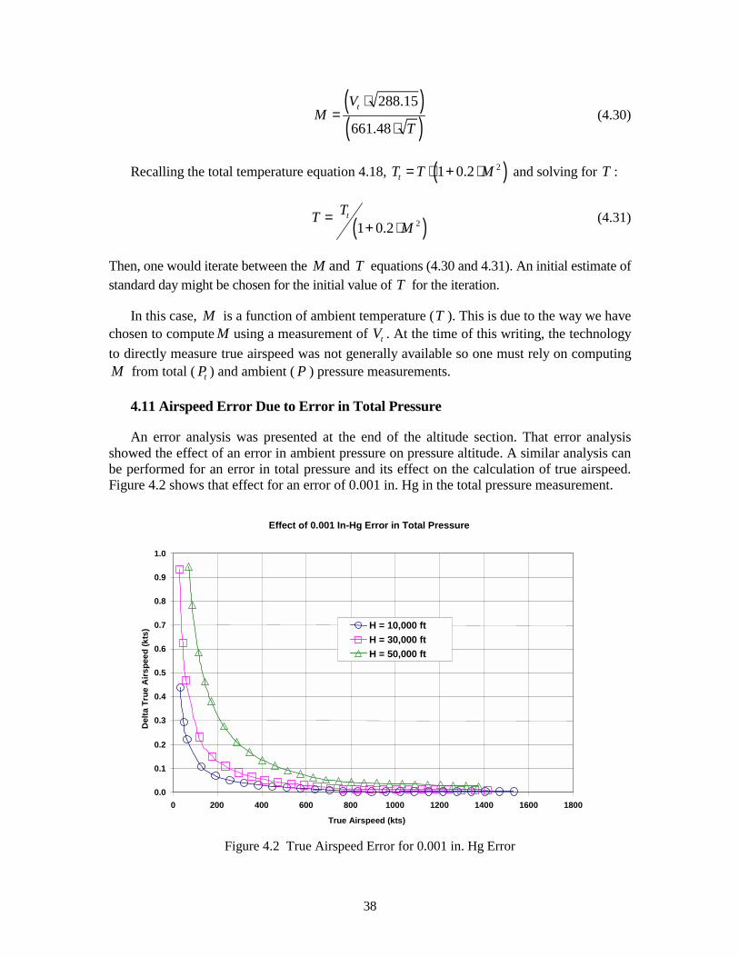
38

( )( )

288.15

661.48tV

MT

⋅=

⋅ (4.30)

Recalling the total temperature equation 4.18, ( )21 0.2tT T M= ⋅ + ⋅ and solving for T :

( )21 0.2tTT

M=

+ ⋅ (4.31)

Then, one would iterate between the andM T equations (4.30 and 4.31). An initial estimate of standard day might be chosen for the initial value of T for the iteration.

In this case, M is a function of ambient temperature (T ). This is due to the way we have chosen to compute M using a measurement of tV . At the time of this writing, the technology to directly measure true airspeed was not generally available so one must rely on computing M from total ( tP ) and ambient ( P ) pressure measurements.

4.11 Airspeed Error Due to Error in Total Pressure

An error analysis was presented at the end of the altitude section. That error analysis showed the effect of an error in ambient pressure on pressure altitude. A similar analysis can be performed for an error in total pressure and its effect on the calculation of true airspeed. Figure 4.2 shows that effect for an error of 0.001 in. Hg in the total pressure measurement.

Effect of 0.001 In-Hg Error in Total Pressure

0.0

0.1

0.2

0.3

0.4

0.5

0.6

0.7

0.8

0.9

1.0

0 200 400 600 800 1000 1200 1400 1600 1800

True Airspeed (kts)

Del

ta T

rue

Airs

peed

(kts

) H = 10,000 ftH = 30,000 ftH = 50,000 ft

Figure 4.2 True Airspeed Error for 0.001 in. Hg Error

39

We have summarized the functional relationships derived in the altitude and airspeed

sections as functions of three basic measurements: total pressure ( tP′ ), ambient (or static) pressure ( P ), and total temperature ( tT ).

a. ( )CH f P= pressure altitude,

b. ( )C CV f q= calibrated airspeed,

c. C tq P P′= − compressible dynamic pressure,

d. ( , )tM f P P′= Mach number. Note that Mach number is obtained without a measurement of temperature,

e. ( , )tT f T M= ambient temperature, and

f. ( , )tV f M T= true airspeed.

40

5.0 LIFT AND DRAG

5.1 Introduction

The aerodynamic force axis system used for aircraft performance is defined by the true airspeed vector. Assuming zero sideslip angle ( β ), the force parallel to true airspeed ( tV ) is the retarding force drag ( D ). Octave Chanute in his 1897 book, Progress in Flying Machines (Reference 5.1), uses the terminology resistance for what we now refer to as drag. The force perpendicular to the true airspeed vector is the lift ( L ) force.

5.2 Definition of Lift and Drag Coefficient Relationships

Lift and drag are referenced to incompressible dynamic pressure and a reference area so that the coefficients are nondimensional. In aircraft applications, the area is a reference wing area. The constants in the following equations are derived from the 1976 U.S. Standard Atmosphere (which are the same as in the 1962 U.S. Standard Atmosphere below 65,000 feet). The lift and drag coefficients are defined as follows:

( )/DC D q S= ⋅ drag coefficient (5.1)

( )/LC L q S= ⋅ lift coefficient (5.2)

where:

D = drag (pounds), L = lift (pounds), q = incompressible dynamic pressure (pounds/feet²), and S = reference wing area (feet²).

Defining q :

2 20.5 0.7tq V P Mρ= ⋅ ⋅ = ⋅ ⋅ (5.3)

To show how the above equivalence is developed, we use formulas we previously derived.

a. ( )P

R Tρ = ⋅ ,

b. tV R T Mγ= ⋅ ⋅ ⋅ , and

c. ( ) ( )2 20.5 0.5 0.5 1.4 0.7tPq V R T M M P M

R Tρ γ= ⋅ ⋅ = ⋅ ⋅ ⋅ ⋅ = ⋅ ⋅ = ⋅ ⋅

⋅.

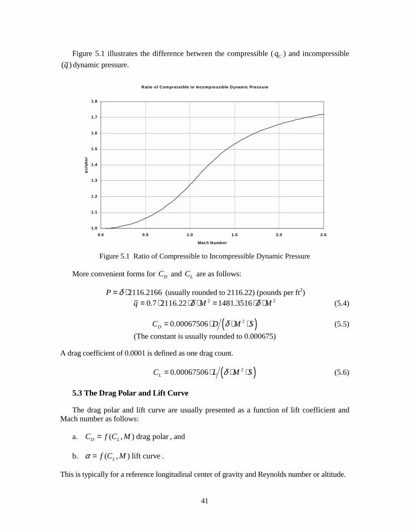
41

Figure 5.1 illustrates the difference between the compressible ( Cq ) and incompressible ( )q dynamic pressure.

Ratio of Compressible to Incompressible Dynamic Pressure

1.0

1.1

1.2

1.3

1.4

1.5

1.6

1.7

1.8

0.0 0.5 1.0 1.5 2.0 2 .5

Mach Number

qc/

qbar

Figure 5.1 Ratio of Compressible to Incompressible Dynamic Pressure

More convenient forms for DC and LC are as follows:

2116.2166P δ= ⋅ (usually rounded to 2116.22) (pounds per ft2) 2 20.7 2116.22 1481.3516q M Mδ δ= ⋅ ⋅ ⋅ = ⋅ ⋅ (5.4)

( )20.00067506DC D M Sδ= ⋅ ⋅ ⋅ (5.5) (The constant is usually rounded to 0.000675)

A drag coefficient of 0.0001 is defined as one drag count.

( )20.00067506LC L M Sδ= ⋅ ⋅ ⋅ (5.6)

5.3 The Drag Polar and Lift Curve

The drag polar and lift curve are usually presented as a function of lift coefficient and Mach number as follows:

a. ( , ) drag polarD LC f C M= , and

b. ( , ) lift curveLf C Mα = .

This is typically for a reference longitudinal center of gravity and Reynolds number or altitude.

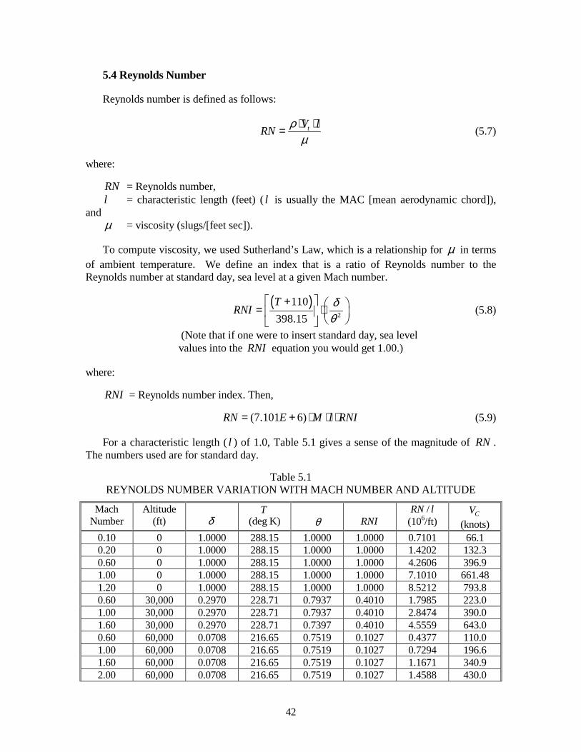
42

5.4 Reynolds Number

Reynolds number is defined as follows:

tV lRN ρµ⋅ ⋅= (5.7)

where:

RN = Reynolds number, l = characteristic length (feet) ( l is usually the MAC [mean aerodynamic chord]),

and µ = viscosity (slugs/[feet sec]).

To compute viscosity, we used Sutherland’s Law, which is a relationship for µ in terms of ambient temperature. We define an index that is a ratio of Reynolds number to the Reynolds number at standard day, sea level at a given Mach number.

( )

2

110398.15T

RNI δθ

+ = ⋅

(5.8)

(Note that if one were to insert standard day, sea level values into the RNI equation you would get 1.00.)

where:

RNI = Reynolds number index. Then,

(7.101 6)RN E M l RNI= + ⋅ ⋅ ⋅ (5.9)

For a characteristic length ( l ) of 1.0, Table 5.1 gives a sense of the magnitude of RN . The numbers used are for standard day.

Table 5.1 REYNOLDS NUMBER VARIATION WITH MACH NUMBER AND ALTITUDE

Mach Number

Altitude (ft)

δ

T (deg K)

θ

RNI

/RN l (106/ft)

CV (knots)

0.10 0 1.0000 288.15 1.0000 1.0000 0.7101 66.1 0.20 0 1.0000 288.15 1.0000 1.0000 1.4202 132.3 0.60 0 1.0000 288.15 1.0000 1.0000 4.2606 396.9 1.00 0 1.0000 288.15 1.0000 1.0000 7.1010 661.48 1.20 0 1.0000 288.15 1.0000 1.0000 8.5212 793.8 0.60 30,000 0.2970 228.71 0.7937 0.4010 1.7985 223.0 1.00 30,000 0.2970 228.71 0.7937 0.4010 2.8474 390.0 1.60 30,000 0.2970 228.71 0.7397 0.4010 4.5559 643.0 0.60 60,000 0.0708 216.65 0.7519 0.1027 0.4377 110.0 1.00 60,000 0.0708 216.65 0.7519 0.1027 0.7294 196.6 1.60 60,000 0.0708 216.65 0.7519 0.1027 1.1671 340.9 2.00 60,000 0.0708 216.65 0.7519 0.1027 1.4588 430.0

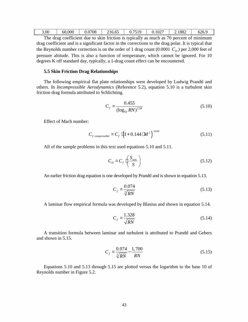
43

3.00 60,000 0.0708 216.65 0.7519 0.1027 2.1882 626.9 The drag coefficient due to skin friction is typically as much as 70 percent of minimum

drag coefficient and is a significant factor in the corrections to the drag polar. It is typical that the Reynolds number correction is on the order of 1 drag count (0.0001 DC ) per 2,000 feet of pressure altitude. This is also a function of temperature, which cannot be ignored. For 10 degrees K off standard day, typically, a 1-drag count effect can be encountered.

5.5 Skin Friction Drag Relationships

The following empirical flat plate relationships were developed by Ludwig Prandtl and others. In Incompressible Aerodynamics (Reference 5.2), equation 5.10 is a turbulent skin friction drag formula attributed to Schlichting.

2.5810

0.455(log )fC

RN= (5.10)

Effect of Mach number:

( ) 0.6521 0.144f compressible fC C M−

= ⋅ + ⋅ (5.11)

All of the sample problems in this text used equations 5.10 and 5.11.

wetD f

SC CS

= ⋅

(5.12)

An earlier friction drag equation is one developed by Prandtl and is shown in equation 5.13.

5

0.074fC

RN= (5.13)

A laminar flow empirical formula was developed by Blasius and shown in equation 5.14.

1.328fC

RN= (5.14)

A transition formula between laminar and turbulent is attributed to Prandtl and Gebers and shown in 5.15.

5

0.074 1,700fC

RNRN= − (5.15)

Equations 5.10 and 5.13 through 5.15 are plotted versus the logarithm to the base 10 of Reynolds number in Figure 5.2.

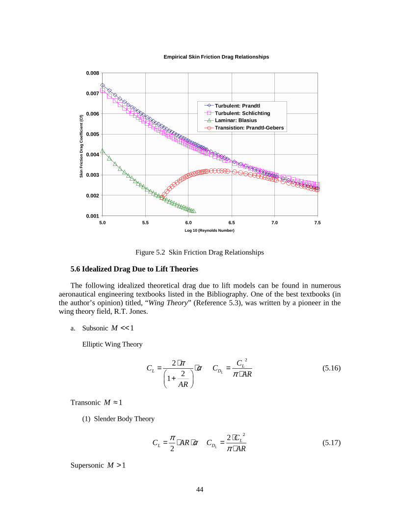
44

Empirical Skin Friction Drag Relationships

0.001

0.002

0.003

0.004

0.005

0.006

0.007

0.008

5.0 5.5 6.0 6.5 7.0 7.5Log 10 (Reynolds Number)

Skin

Fric

tion

Dra

g C

oeffi

cien

t (C

f)

Turbulent: PrandtlTurbulent: SchlichtingLaminar: BlasiusTransistion: Prandtl-Gebers

Figure 5.2 Skin Friction Drag Relationships

5.6 Idealized Drag Due to Lift Theories

The following idealized theoretical drag due to lift models can be found in numerous aeronautical engineering textbooks listed in the Bibliography. One of the best textbooks (in the author’s opinion) titled, “Wing Theory” (Reference 5.3), was written by a pioneer in the wing theory field, R.T. Jones.

a. Subsonic 1M <<

Elliptic Wing Theory

22

21L

LL D

CC CAR

AR

π απ

⋅= ⋅ =⋅ +

(5.16)

Transonic 1M ≈

(1) Slender Body Theory

22

2 L

LL D

CC AR CAR

π απ⋅= ⋅ ⋅ =⋅

(5.17)

Supersonic 1M >

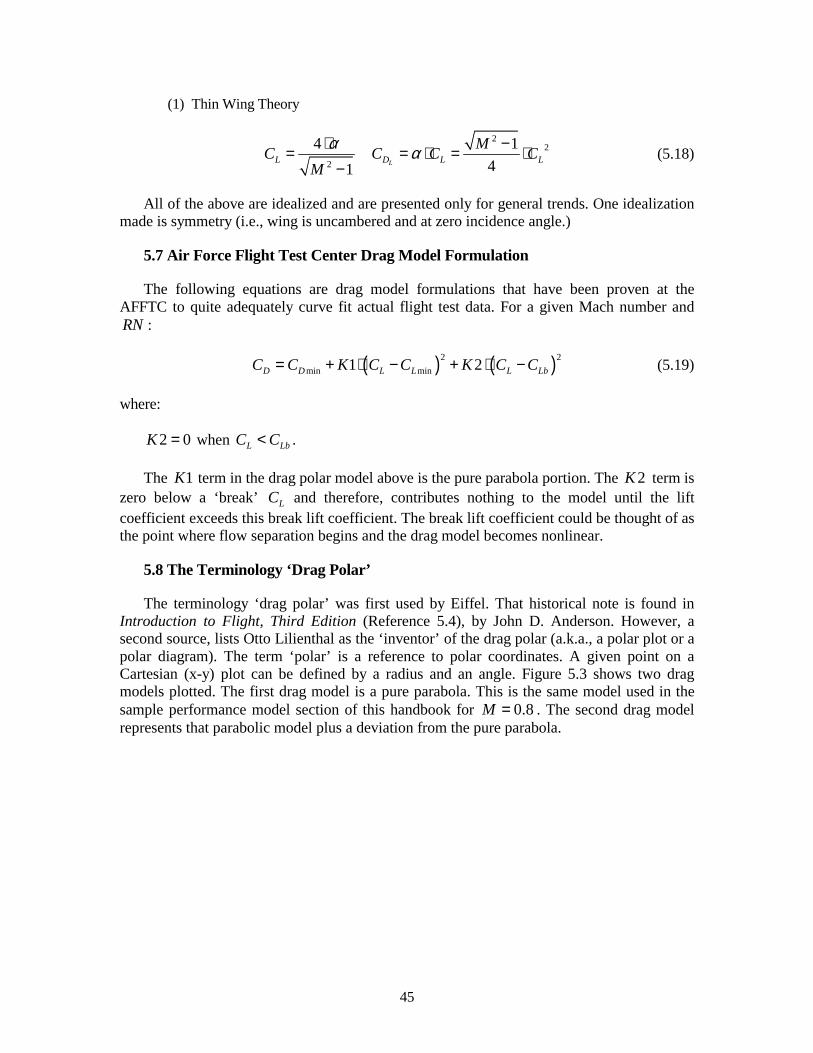
45

(1) Thin Wing Theory

2

2

2

4 141 LL D L L

MC C C CMα α⋅ −= = ⋅ = ⋅−

(5.18)

All of the above are idealized and are presented only for general trends. One idealization made is symmetry (i.e., wing is uncambered and at zero incidence angle.)

5.7 Air Force Flight Test Center Drag Model Formulation

The following equations are drag model formulations that have been proven at the AFFTC to quite adequately curve fit actual flight test data. For a given Mach number and RN :

( ) ( )2 2min min1 2D D L L L LbC C K C C K C C= + ⋅ − + ⋅ − (5.19)

where:

2 0K = when L LbC C< .

The 1K term in the drag polar model above is the pure parabola portion. The 2K term is zero below a ‘break’ LC and therefore, contributes nothing to the model until the lift coefficient exceeds this break lift coefficient. The break lift coefficient could be thought of as the point where flow separation begins and the drag model becomes nonlinear.

5.8 The Terminology ‘Drag Polar’

The terminology ‘drag polar’ was first used by Eiffel. That historical note is found in Introduction to Flight, Third Edition (Reference 5.4), by John D. Anderson. However, a second source, lists Otto Lilienthal as the ‘inventor’ of the drag polar (a.k.a., a polar plot or a polar diagram). The term ‘polar’ is a reference to polar coordinates. A given point on a Cartesian (x-y) plot can be defined by a radius and an angle. Figure 5.3 shows two drag models plotted. The first drag model is a pure parabola. This is the same model used in the sample performance model section of this handbook for 0.8M = . The second drag model represents that parabolic model plus a deviation from the pure parabola.

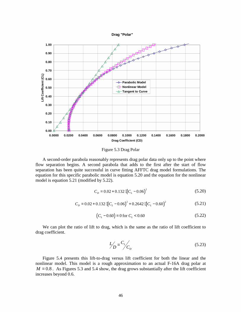
46

Drag "Polar"

0.00

0.10

0.20

0.30

0.40

0.50

0.60

0.70

0.80

0.90

1.00

0.0000 0.0200 0.0400 0.0600 0.0800 0.1000 0.1200 0.1400 0.1600 0.1800 0.2000Drag Coefficient (CD)

Lift

Coe

ffici

ent (

CL)

Parabolic ModelNonlinear ModelTangent to Curve

Figure 5.3 Drag Polar

A second-order parabola reasonably represents drag polar data only up to the point where flow separation begins. A second parabola that adds to the first after the start of flow separation has been quite successful in curve fitting AFFTC drag model formulations. The equation for this specific parabolic model is equation 5.20 and the equation for the nonlinear model is equation 5.21 (modified by 5.22).

( )20.02 0.132 0.06D LC C= + ⋅ − (5.20)

( ) ( )2 20.02 0.132 0.06 0.2642 0.60D L LC C C= + ⋅ − + ⋅ − (5.21)

( )0.60 0 for 0.60L LC C− = < (5.22)

We can plot the ratio of lift to drag, which is the same as the ratio of lift coefficient to drag coefficient.

L

D

CLD C= (5.23)

Figure 5.4 presents this lift-to-drag versus lift coefficient for both the linear and the nonlinear model. This model is a rough approximation to an actual F-16A drag polar at

0.8M = . As Figures 5.3 and 5.4 show, the drag grows substantially after the lift coefficient increases beyond 0.6.

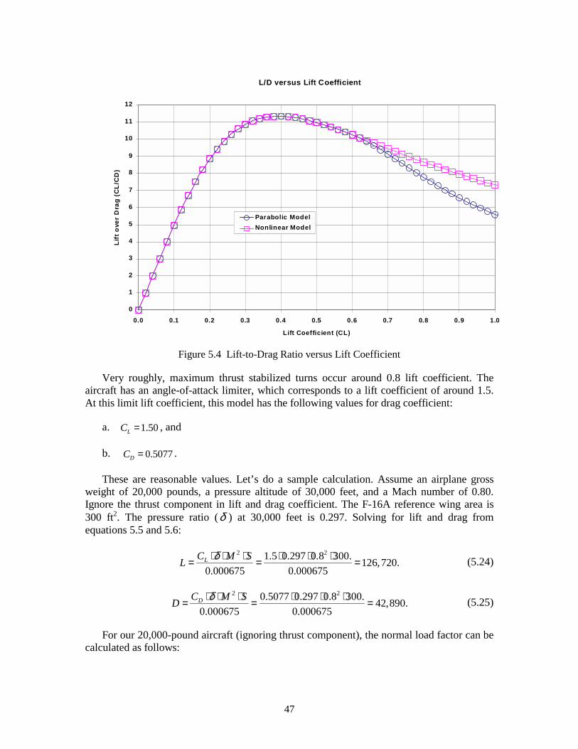
47

L/D versus Lift Coefficient

0

1

2

3

4

5

6

7

8

9

10

11

12

0.0 0.1 0.2 0.3 0.4 0.5 0.6 0.7 0.8 0.9 1.0

Lift Coefficient (CL)

Lift

ove

r D

rag

(CL

/CD

)

Parabolic ModelNonlinear Model

Figure 5.4 Lift-to-Drag Ratio versus Lift Coefficient

Very roughly, maximum thrust stabilized turns occur around 0.8 lift coefficient. The aircraft has an angle-of-attack limiter, which corresponds to a lift coefficient of around 1.5. At this limit lift coefficient, this model has the following values for drag coefficient:

a. 1.50LC = , and

b. 0.5077DC = .

These are reasonable values. Let’s do a sample calculation. Assume an airplane gross weight of 20,000 pounds, a pressure altitude of 30,000 feet, and a Mach number of 0.80. Ignore the thrust component in lift and drag coefficient. The F-16A reference wing area is 300 ft2. The pressure ratio (δ ) at 30,000 feet is 0.297. Solving for lift and drag from equations 5.5 and 5.6:

2 21.5 0.297 0.8 300. 126,720.

0.000675 0.000675LC M SL δ⋅ ⋅ ⋅ ⋅ ⋅ ⋅= = = (5.24)

2 20.5077 0.297 0.8 300. 42,890.

0.000675 0.000675DC M SD δ⋅ ⋅ ⋅ ⋅ ⋅ ⋅= = = (5.25)

For our 20,000-pound aircraft (ignoring thrust component), the normal load factor can be calculated as follows:

48

126,720.126,720. 6.34 g's20,000.z t zL N W N= ⋅ = → = =

Let’s say that someone told us that the aircraft could sustain 4.5 g’s in maximum afterburner at these conditions. Since thrust equals drag in a sustained (or thrust-limited) turn, we can calculate the drag by first calculating the lift coefficient.

2 2

0.000675 0.000675 4.5 20,000. 1.070.297 0.8 300.

z tL

N WCM Sδ

⋅ ⋅ ⋅ ⋅= = =⋅ ⋅ ⋅ ⋅

(5.26)

From the drag polar equation (5.21), the drag coefficient comes to 0.2130. Solving for drag (which is equal to net thrust):

2 20.2130 0.297 0.8 300. 17,994.

0.000675 0.000675DC M SD δ⋅ ⋅ ⋅ ⋅ ⋅ ⋅= = = (5.27)

At the maximum lift point, the excess thrust is:

17,994. 42,890. 24,895.ex nF F D= − = − = − (5.28)

That would be a longitudinal load factor of greater than a -1 g. The deceleration rate in knots per second comes to:

0

24,895. 1.2520,000.

tx

t

VhN V g−= = − = +

!! (5.29)

Assuming all the negative excess thrust is in deceleration (constant altitude slow down turn):

( ) ( )2ft1.25 32.174 sec knots23.8 secft

sec1.6878 knot

tV− ⋅

= = −

! (5.30)

SECTION 5.0 REFERENCES

5.1 Chanute, Octave. 1897. Progress in Flying Machines, The American Engineer and Railroad Journal.

5.2 Twaites, Bryan, ed. 1960. Incompressible Aerodynamics: An Account of the Steady Flow of

Incompressible Fluid past Aerofoils, Wings, and other Bodies. Dover Publications. 5.3 Jones, Robert T. 1990. Wing Theory. Princeton University Press. 5.4 Anderson, John D. 1989. Introduction to Flight, Third Edition. New York, New York:

McGraw-Hill, Inc.

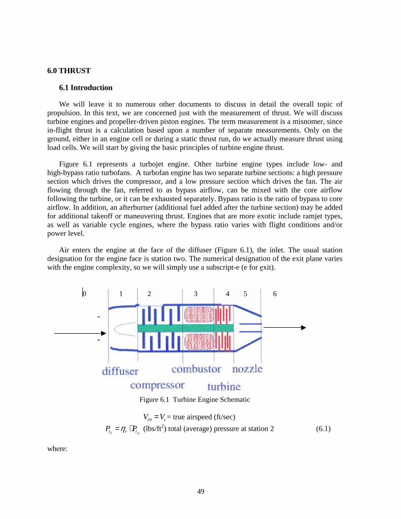
6.0 THRUST

6.1 Introduction

We will leave it to numerous other documents to discuss in detail the overall topic of propulsion. In this text, we are concerned just with the measurement of thrust. We will discuss turbine engines and propeller-driven piston engines. The term measurement is a misnomer, since in-flight thrust is a calculation based upon a number of separate measurements. Only on the ground, either in an engine cell or during a static thrust run, do we actually measure thrust using load cells. We will start by giving the basic principles of turbine engine thrust.

Figure 6.1 represents a turbojet engine. Other turbine engine types include low- and high-bypass ratio turbofans. A turbofan engine has two separate turbine sections: a high pressure section which drives the compressor, and a low pressure section which drives the fan. The air flowing through the fan, referred to as bypass airflow, can be mixed with the core airflow following the turbine, or it can be exhausted separately. Bypass ratio is the ratio of bypass to core airflow. In addition, an afterburner (additional fuel added after the turbine section) may be added for additional takeoff or maneuvering thrust. Engines that are more exotic include ramjet types, as well as variable cycle engines, where the bypass ratio varies with flight conditions and/or power level.

Air enters the engine at the face of the diffuser (Figure 6.1), the inlet. The usual station designation for the engine face is station two. The numerical designation of the exit plane varies with the engine complexity, so we will simply use a subscript-e (e for exit).

Figure 6.1 Turb

0t tV V= = true

2 0t r tP Pη= ⋅ (lbs/ft2) total (

where:

0 1 2 4 5 6
3
49

ine Engine Schematic

airspeed (ft/sec) average) pressure at station 2 (6.1)

50

rη = inlet recovery factor (addressed in more detail later), and

0tP = free stream total (average) pressure (lbs/ft2).

( )0

3.521 0.2tP P M= ⋅ + ⋅ ( pounds/ft2) (6.2)

where:

P =ambient pressure (lbs/ft2).

Note: All of the velocities and pressures are integrated average values.

6.2 The Thrust Equation

The net propulsive force on the vehicle is called net thrust ( nF ). The basic thrust equation is gross thrust ( gF ) minus ram drag ( rF ). The gross thrust, in layman’s terms, is thrust out the back. Ram drag is the result of slowing the air from free stream to near zero speed at the inlet. The term ( )e eA P P⋅ − in the equation for gross thrust, 6.4 below, is the result of the pressure at the exhaust plane being higher, in most cases, than the ambient pressure. However, this is generally a small term compared to the ( )a f eW W V+ ⋅! term.

n g rF F F= − (6.3)

( ) ( )g a f e e eF W W V A P P= + ⋅ + ⋅ −! (6.4)

r a tF W V= ⋅! (6.5)

where:

aW! = airflow rate (lbs/sec) through the engine,

fW = fuel flow (lbs/sec),

eV = exit velocity (ft/sec) (average),

eP = pressure (average) across exit plane (lbs/ft2), and

eA = cross sectional area of the exit nozzle (ft2). For turbofan engines an additional pressure times area term must be added to equation 6.4

when the fan thrust is exhausted separately. Previously defined was the fuel flow ( fW ), however, now we will think of it in units of pounds per second to be consistent with the airflow rate. Note that the total mass flow into the engine is airflow, while exiting the engine mass flow is airflow plus fuel flow. A more precise engine thrust computation would take into account various bleed airs that extract air off the engine for cooling and other purposes.

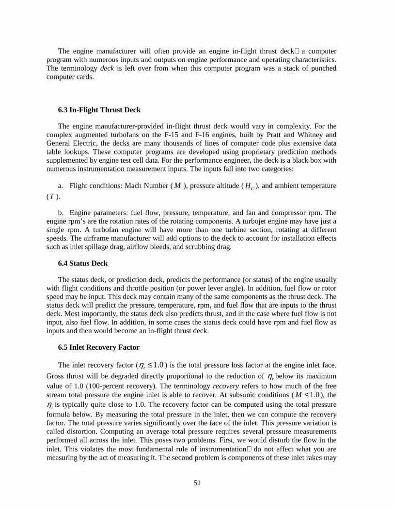
51

The engine manufacturer will often provide an engine in-flight thrust deck a computer program with numerous inputs and outputs on engine performance and operating characteristics. The terminology deck is left over from when this computer program was a stack of punched computer cards.

6.3 In-Flight Thrust Deck

The engine manufacturer-provided in-flight thrust deck would vary in complexity. For the complex augmented turbofans on the F-15 and F-16 engines, built by Pratt and Whitney and General Electric, the decks are many thousands of lines of computer code plus extensive data table lookups. These computer programs are developed using proprietary prediction methods supplemented by engine test cell data. For the performance engineer, the deck is a black box with numerous instrumentation measurement inputs. The inputs fall into two categories:

a. Flight conditions: Mach Number ( M ), pressure altitude ( CH ), and ambient temperature (T ).

b. Engine parameters: fuel flow, pressure, temperature, and fan and compressor rpm. The engine rpm’s are the rotation rates of the rotating components. A turbojet engine may have just a single rpm. A turbofan engine will have more than one turbine section, rotating at different speeds. The airframe manufacturer will add options to the deck to account for installation effects such as inlet spillage drag, airflow bleeds, and scrubbing drag.

6.4 Status Deck

The status deck, or prediction deck, predicts the performance (or status) of the engine usually with flight conditions and throttle position (or power lever angle). In addition, fuel flow or rotor speed may be input. This deck may contain many of the same components as the thrust deck. The status deck will predict the pressure, temperature, rpm, and fuel flow that are inputs to the thrust deck. Most importantly, the status deck also predicts thrust, and in the case where fuel flow is not input, also fuel flow. In addition, in some cases the status deck could have rpm and fuel flow as inputs and then would become an in-flight thrust deck.

6.5 Inlet Recovery Factor

The inlet recovery factor ( 1.0rη ≤ ) is the total pressure loss factor at the engine inlet face. Gross thrust will be degraded directly proportional to the reduction of rη below its maximum value of 1.0 (100-percent recovery). The terminology recovery refers to how much of the free stream total pressure the engine inlet is able to recover. At subsonic conditions ( 1.0M < ), the

rη is typically quite close to 1.0. The recovery factor can be computed using the total pressure formula below. By measuring the total pressure in the inlet, then we can compute the recovery factor. The total pressure varies significantly over the face of the inlet. This pressure variation is called distortion. Computing an average total pressure requires several pressure measurements performed all across the inlet. This poses two problems. First, we would disturb the flow in the inlet. This violates the most fundamental rule of instrumentation do not affect what you are measuring by the act of measuring it. The second problem is components of these inlet rakes may

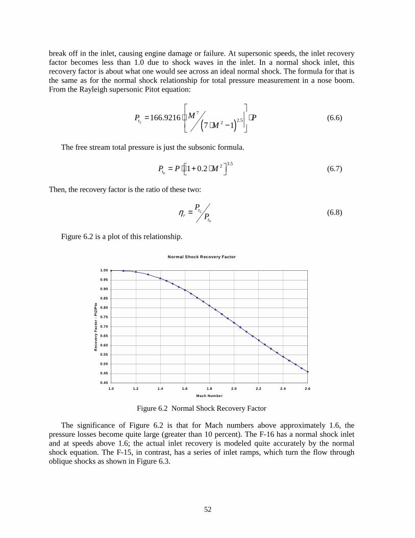
52

break off in the inlet, causing engine damage or failure. At supersonic speeds, the inlet recovery factor becomes less than 1.0 due to shock waves in the inlet. In a normal shock inlet, this recovery factor is about what one would see across an ideal normal shock. The formula for that is the same as for the normal shock relationship for total pressure measurement in a nose boom. From the Rayleigh supersonic Pitot equation:

( )2

72.52

166.92167 1

tMP P

M

= ⋅ ⋅ ⋅ −

(6.6)

The free stream total pressure is just the subsonic formula.

0

3.521 0.2tP P M = ⋅ + ⋅ (6.7)

Then, the recovery factor is the ratio of these two:

2

0

tr

t

PPη = (6.8)

Figure 6.2 is a plot of this relationship.

Normal Shock Recovery Factor

0.40

0.45

0.50

0.55

0.60

0.65

0.70

0.75

0.80

0.85

0.90

0.95

1.00

1.0 1.2 1.4 1.6 1.8 2.0 2.2 2.4 2.6

Mach Number

Rec

ove

ry F

acto

r -

Pt2

/Pto

Figure 6.2 Normal Shock Recovery Factor

The significance of Figure 6.2 is that for Mach numbers above approximately 1.6, the pressure losses become quite large (greater than 10 percent). The F-16 has a normal shock inlet and at speeds above 1.6; the actual inlet recovery is modeled quite accurately by the normal shock equation. The F-15, in contrast, has a series of inlet ramps, which turn the flow through oblique shocks as shown in Figure 6.3.

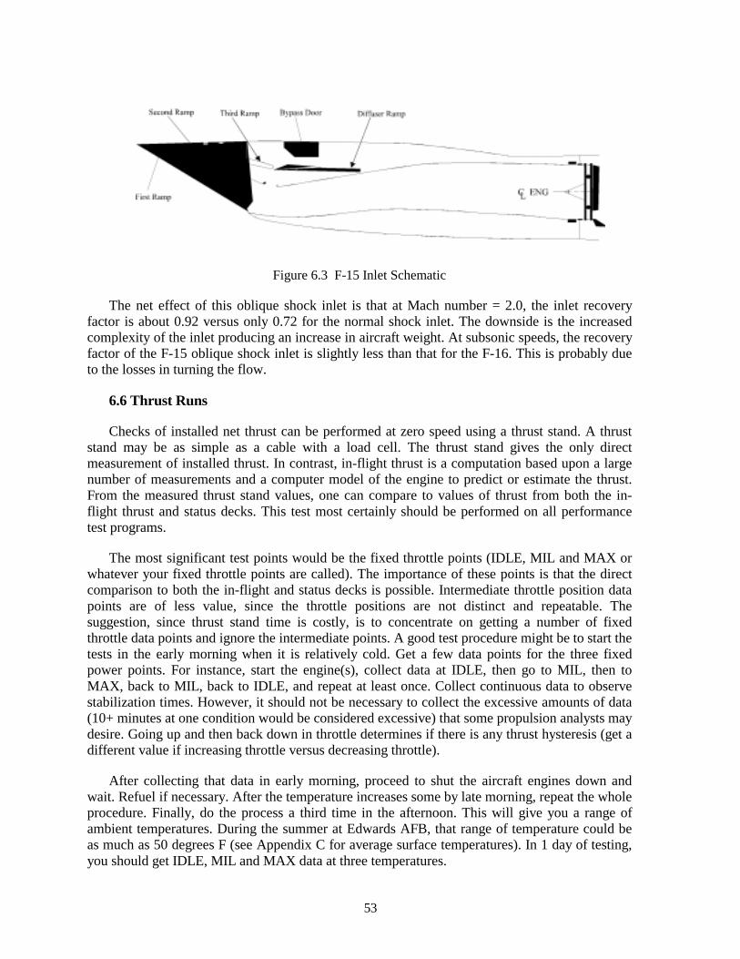
53

Figure 6.3 F-15 Inlet Schematic

The net effect of this oblique shock inlet is that at Mach number = 2.0, the inlet recovery factor is about 0.92 versus only 0.72 for the normal shock inlet. The downside is the increased complexity of the inlet producing an increase in aircraft weight. At subsonic speeds, the recovery factor of the F-15 oblique shock inlet is slightly less than that for the F-16. This is probably due to the losses in turning the flow.

6.6 Thrust Runs

Checks of installed net thrust can be performed at zero speed using a thrust stand. A thrust stand may be as simple as a cable with a load cell. The thrust stand gives the only direct measurement of installed thrust. In contrast, in-flight thrust is a computation based upon a large number of measurements and a computer model of the engine to predict or estimate the thrust. From the measured thrust stand values, one can compare to values of thrust from both the in-flight thrust and status decks. This test most certainly should be performed on all performance test programs.

The most significant test points would be the fixed throttle points (IDLE, MIL and MAX or whatever your fixed throttle points are called). The importance of these points is that the direct comparison to both the in-flight and status decks is possible. Intermediate throttle position data points are of less value, since the throttle positions are not distinct and repeatable. The suggestion, since thrust stand time is costly, is to concentrate on getting a number of fixed throttle data points and ignore the intermediate points. A good test procedure might be to start the tests in the early morning when it is relatively cold. Get a few data points for the three fixed power points. For instance, start the engine(s), collect data at IDLE, then go to MIL, then to MAX, back to MIL, back to IDLE, and repeat at least once. Collect continuous data to observe stabilization times. However, it should not be necessary to collect the excessive amounts of data (10+ minutes at one condition would be considered excessive) that some propulsion analysts may desire. Going up and then back down in throttle determines if there is any thrust hysteresis (get a different value if increasing throttle versus decreasing throttle).

After collecting that data in early morning, proceed to shut the aircraft engines down and wait. Refuel if necessary. After the temperature increases some by late morning, repeat the whole procedure. Finally, do the process a third time in the afternoon. This will give you a range of ambient temperatures. During the summer at Edwards AFB, that range of temperature could be as much as 50 degrees F (see Appendix C for average surface temperatures). In 1 day of testing, you should get IDLE, MIL and MAX data at three temperatures.

54

6.7 Thrust Dynamics

In an engine test cell, the engine manufacturer will perform throttle transients. This data can be used to develop a thrust dynamics model for use with a takeoff simulation. The typical aircraft is unable to stabilize at the start of a takeoff with maximum thrust. Therefore, a throttle transient is necessary to initiate the takeoff. Figure 6.4 is an example of some actual throttle transient data taken on the AFFTC thrust stand.

Thrust Lag versus Time

-10

0

10

20

30

40

50

60

70

80

90

100

0 2 4 6 8 10 12 14

Elapsed Time (sec)

Perc

ent C

hang

e in

Thr

ust [

MIL

to M

AX]

Figure 6.4 Thrust Dynamics from an Air Force Flight Test Center Thrust Stand

The thrust stand at the time this data was taken (late 1980s) had a 1 sample per second sample rate. In addition, it is unknown how much of the lag is due to lag in the instrumentation. However, using this thrust stand lag data allowed us to match the actual time to liftoff data very accurately. As an example, for this aircraft, the time to lift-off at one particular condition was 41.5 seconds using the simulation. For the same simulation, but assuming 100 percent thrust at time zero, the time to lift-off was computed to be 39.1 seconds (or over 5 percent). The change in distance to lift-off, for the same lift-off speed, was less than 1 percent. To clarify, the effect of the engine lag occurs in the early portion of the takeoff ground roll, affecting time to takeoff much more than distance to liftoff. This becomes significant when considering minimum interval takeoffs, for instance.

6.8 Propeller Thrust

In the examples, it was assumed that thrust was derived from a jet engine. We do not wish to assume that is always the case. The equations of motion are just as applicable to an aircraft powered by an engine that drives a propeller. The common unit of output power of an engine is horsepower. In the English system, 1 horsepower was defined by James Watt in the 1700s to

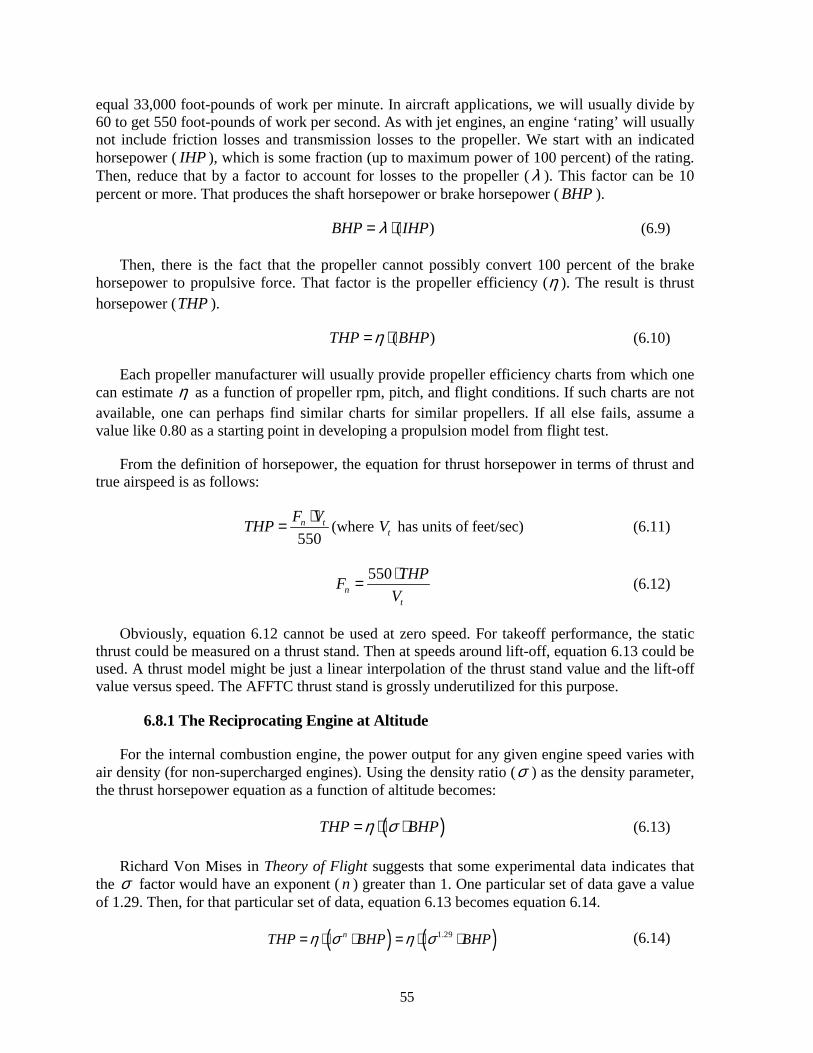
55

equal 33,000 foot-pounds of work per minute. In aircraft applications, we will usually divide by 60 to get 550 foot-pounds of work per second. As with jet engines, an engine ‘rating’ will usually not include friction losses and transmission losses to the propeller. We start with an indicated horsepower ( IHP ), which is some fraction (up to maximum power of 100 percent) of the rating. Then, reduce that by a factor to account for losses to the propeller (λ ). This factor can be 10 percent or more. That produces the shaft horsepower or brake horsepower ( BHP ).

( )BHP IHPλ= ⋅ (6.9)

Then, there is the fact that the propeller cannot possibly convert 100 percent of the brake horsepower to propulsive force. That factor is the propeller efficiency (η ). The result is thrust horsepower (THP ).

( )THP BHPη= ⋅ (6.10)

Each propeller manufacturer will usually provide propeller efficiency charts from which one can estimate η as a function of propeller rpm, pitch, and flight conditions. If such charts are not available, one can perhaps find similar charts for similar propellers. If all else fails, assume a value like 0.80 as a starting point in developing a propulsion model from flight test.

From the definition of horsepower, the equation for thrust horsepower in terms of thrust and true airspeed is as follows:

550n tF VTHP ⋅= (where tV has units of feet/sec) (6.11)

550n

t

THPFV⋅= (6.12)

Obviously, equation 6.12 cannot be used at zero speed. For takeoff performance, the static thrust could be measured on a thrust stand. Then at speeds around lift-off, equation 6.13 could be used. A thrust model might be just a linear interpolation of the thrust stand value and the lift-off value versus speed. The AFFTC thrust stand is grossly underutilized for this purpose.

6.8.1 The Reciprocating Engine at Altitude

For the internal combustion engine, the power output for any given engine speed varies with air density (for non-supercharged engines). Using the density ratio (σ ) as the density parameter, the thrust horsepower equation as a function of altitude becomes:

( )THP BHPη σ= ⋅ ⋅ (6.13)

Richard Von Mises in Theory of Flight suggests that some experimental data indicates that the σ factor would have an exponent ( n ) greater than 1. One particular set of data gave a value of 1.29. Then, for that particular set of data, equation 6.13 becomes equation 6.14.

( ) ( )1.29nTHP BHP BHPη σ η σ= ⋅ ⋅ = ⋅ ⋅ (6.14)

56

For instance, for an engine at 20,000 feet pressure altitude on a standard day:

a. 0.4595δ = ,

b. 0.8625θ = ,

c. 0.5328δσ θ= = ,

d. 1.29 0.4438σ = , and

e. 1.290.833σ

σ = .

Hence, the altitude degradation factor for this engine is 16.7 percent greater than what would be predicted by a straight density ratio factor.

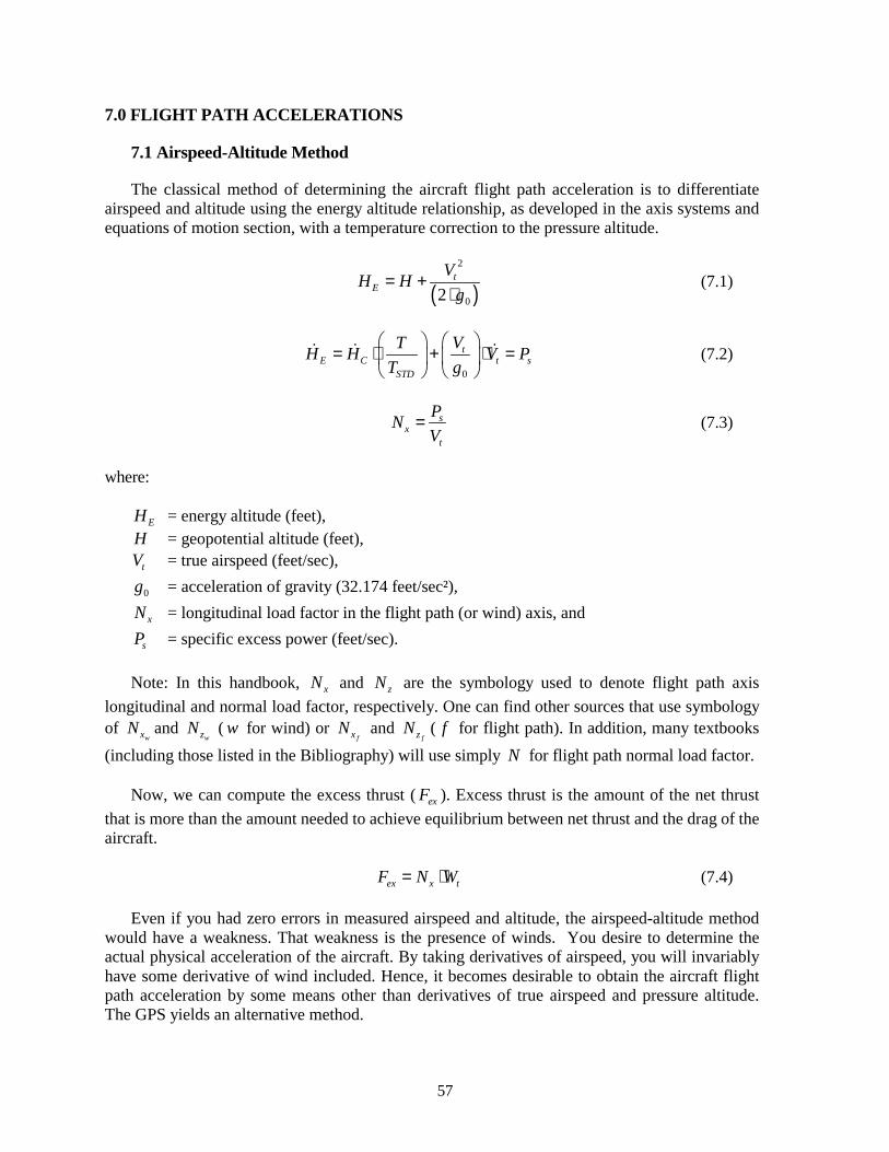
57

7.0 FLIGHT PATH ACCELERATIONS

7.1 Airspeed-Altitude Method

The classical method of determining the aircraft flight path acceleration is to differentiate airspeed and altitude using the energy altitude relationship, as developed in the axis systems and equations of motion section, with a temperature correction to the pressure altitude.

( )2

02t

EVH H

g= +

⋅ (7.1)

0

tE C t s

STD

VTH H V PT g

= ⋅ + ⋅ =

! ! ! (7.2)

sx

t

PNV

= (7.3)

where:

EH = energy altitude (feet), H = geopotential altitude (feet),

tV = true airspeed (feet/sec),

0g = acceleration of gravity (32.174 feet/sec²),

xN = longitudinal load factor in the flight path (or wind) axis, and

sP = specific excess power (feet/sec).

Note: In this handbook, xN and zN are the symbology used to denote flight path axis longitudinal and normal load factor, respectively. One can find other sources that use symbology of

wxN and wzN ( w for wind) or

fxN and fzN ( f for flight path). In addition, many textbooks

(including those listed in the Bibliography) will use simply N for flight path normal load factor.

Now, we can compute the excess thrust ( exF ). Excess thrust is the amount of the net thrust that is more than the amount needed to achieve equilibrium between net thrust and the drag of the aircraft.

ex x tF N W= ⋅ (7.4)

Even if you had zero errors in measured airspeed and altitude, the airspeed-altitude method would have a weakness. That weakness is the presence of winds. You desire to determine the actual physical acceleration of the aircraft. By taking derivatives of airspeed, you will invariably have some derivative of wind included. Hence, it becomes desirable to obtain the aircraft flight path acceleration by some means other than derivatives of true airspeed and pressure altitude. The GPS yields an alternative method.

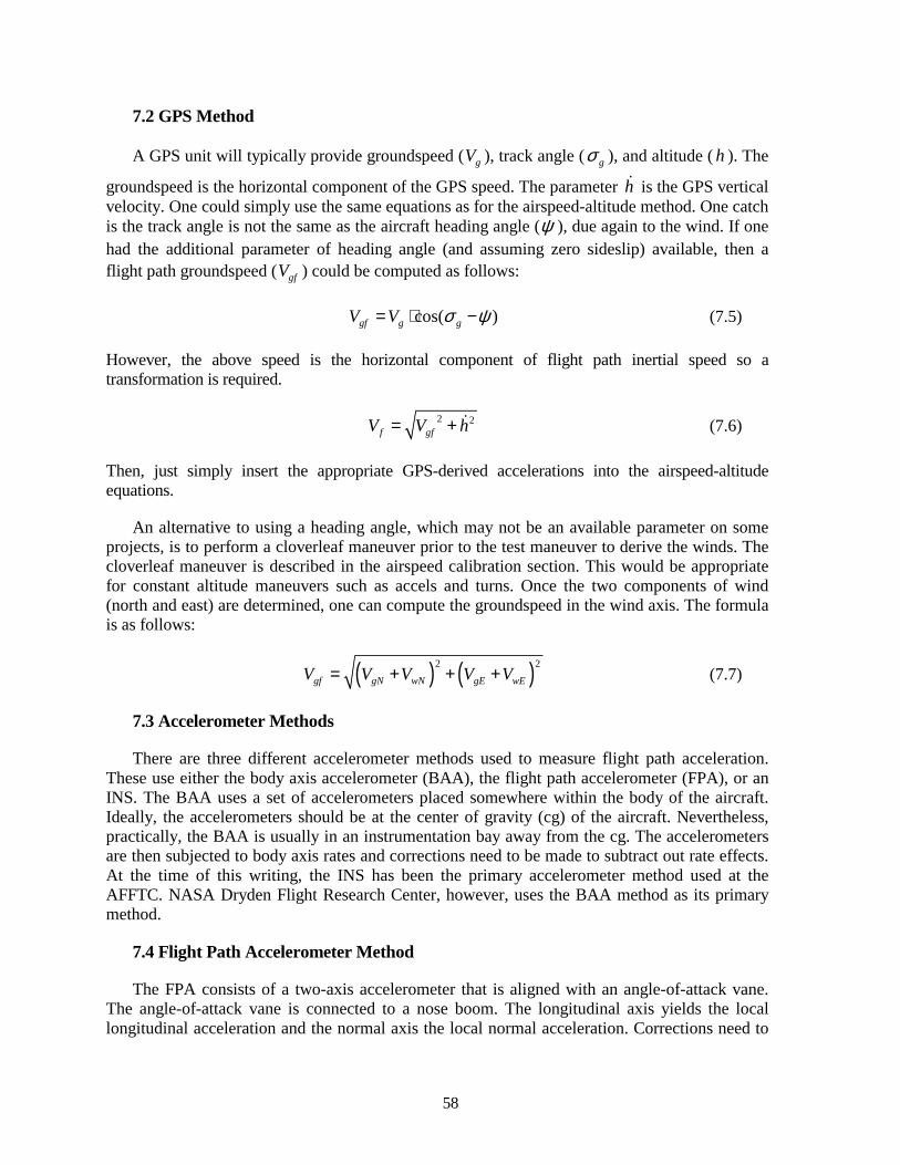
58

7.2 GPS Method

A GPS unit will typically provide groundspeed ( gV ), track angle ( gσ ), and altitude ( h ). The

groundspeed is the horizontal component of the GPS speed. The parameter h! is the GPS vertical velocity. One could simply use the same equations as for the airspeed-altitude method. One catch is the track angle is not the same as the aircraft heading angle (ψ ), due again to the wind. If one had the additional parameter of heading angle (and assuming zero sideslip) available, then a flight path groundspeed ( gfV ) could be computed as follows:

cos( )gf g gV V σ ψ= ⋅ − (7.5)

However, the above speed is the horizontal component of flight path inertial speed so a transformation is required.

2 2f gfV V h= + ! (7.6)

Then, just simply insert the appropriate GPS-derived accelerations into the airspeed-altitude equations.

An alternative to using a heading angle, which may not be an available parameter on some projects, is to perform a cloverleaf maneuver prior to the test maneuver to derive the winds. The cloverleaf maneuver is described in the airspeed calibration section. This would be appropriate for constant altitude maneuvers such as accels and turns. Once the two components of wind (north and east) are determined, one can compute the groundspeed in the wind axis. The formula is as follows:

( ) ( )2 2

gf gN wN gE wEV V V V V= + + + (7.7)

7.3 Accelerometer Methods

There are three different accelerometer methods used to measure flight path acceleration. These use either the body axis accelerometer (BAA), the flight path accelerometer (FPA), or an INS. The BAA uses a set of accelerometers placed somewhere within the body of the aircraft. Ideally, the accelerometers should be at the center of gravity (cg) of the aircraft. Nevertheless, practically, the BAA is usually in an instrumentation bay away from the cg. The accelerometers are then subjected to body axis rates and corrections need to be made to subtract out rate effects. At the time of this writing, the INS has been the primary accelerometer method used at the AFFTC. NASA Dryden Flight Research Center, however, uses the BAA method as its primary method.

7.4 Flight Path Accelerometer Method

The FPA consists of a two-axis accelerometer that is aligned with an angle-of-attack vane. The angle-of-attack vane is connected to a nose boom. The longitudinal axis yields the local longitudinal acceleration and the normal axis the local normal acceleration. Corrections need to

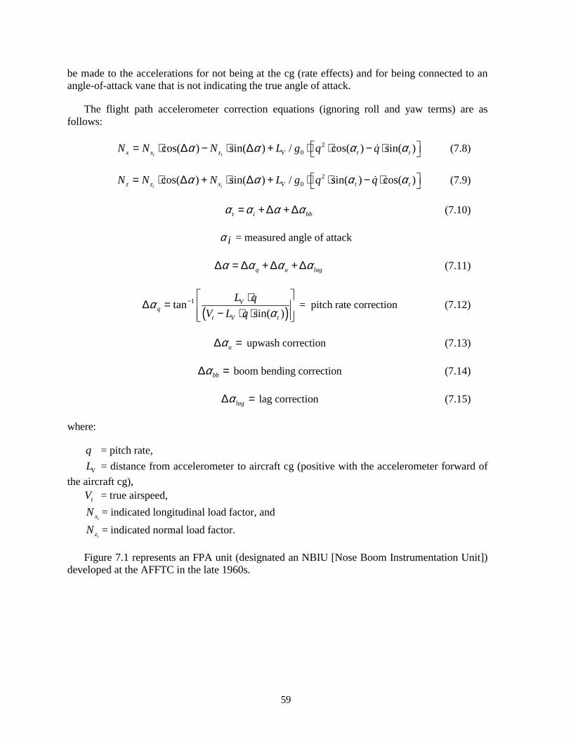
59

be made to the accelerations for not being at the cg (rate effects) and for being connected to an angle-of-attack vane that is not indicating the true angle of attack.

The flight path accelerometer correction equations (ignoring roll and yaw terms) are as follows:

20cos( ) sin( ) / cos( ) sin( )

i ix x z V t tN N N L g q qα α α α = ⋅ ∆ − ⋅ ∆ + ⋅ ⋅ − ⋅ ! (7.8)

20cos( ) sin( ) / sin( ) cos( )

i iz z x V t tN N N L g q qα α α α = ⋅ ∆ + ⋅ ∆ + ⋅ ⋅ − ⋅ ! (7.9)

t i bbα α α α= + ∆ + ∆ (7.10)

α i = measured angle of attack

q u lagα α α α∆ = ∆ + ∆ + ∆ (7.11)

( )

1tansin( )

Vq

t V t

L qV L q

αα

− ⋅∆ = − ⋅ ⋅ = pitch rate correction (7.12)

uα∆ = upwash correction (7.13)

bbα∆ = boom bending correction (7.14)

lagα∆ = lag correction (7.15)

where:

q = pitch rate,

VL = distance from accelerometer to aircraft cg (positive with the accelerometer forward of the aircraft cg),

tV = true airspeed,

ixN = indicated longitudinal load factor, and

izN = indicated normal load factor.

Figure 7.1 represents an FPA unit (designated an NBIU [Nose Boom Instrumentation Unit]) developed at the AFFTC in the late 1960s.

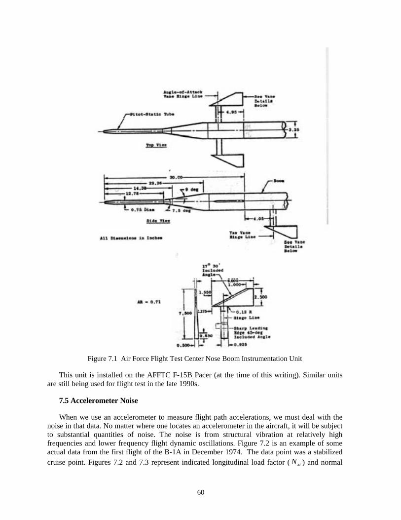
60

Figure 7.1 Air Force Flight Test Center Nose Boom Instrumentation Unit

This unit is installed on the AFFTC F-15B Pacer (at the time of this writing). Similar units are still being used for flight test in the late 1990s.

7.5 Accelerometer Noise

When we use an accelerometer to measure flight path accelerations, we must deal with the noise in that data. No matter where one locates an accelerometer in the aircraft, it will be subject to substantial quantities of noise. The noise is from structural vibration at relatively high frequencies and lower frequency flight dynamic oscillations. Figure 7.2 is an example of some actual data from the first flight of the B-1A in December 1974. The data point was a stabilized cruise point. Figures 7.2 and 7.3 represent indicated longitudinal load factor ( xiN ) and normal

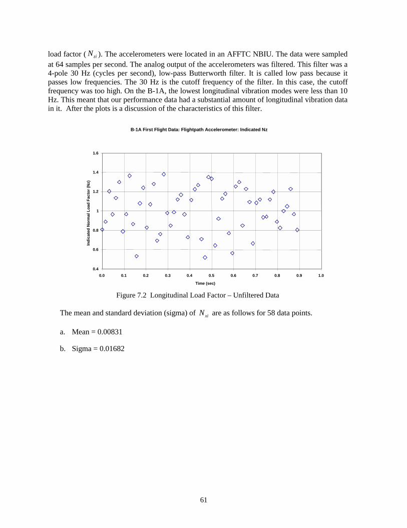
61

load factor ( ziN ). The accelerometers were located in an AFFTC NBIU. The data were sampled at 64 samples per second. The analog output of the accelerometers was filtered. This filter was a 4-pole 30 Hz (cycles per second), low-pass Butterworth filter. It is called low pass because it passes low frequencies. The 30 Hz is the cutoff frequency of the filter. In this case, the cutoff frequency was too high. On the B-1A, the lowest longitudinal vibration modes were less than 10 Hz. This meant that our performance data had a substantial amount of longitudinal vibration data in it. After the plots is a discussion of the characteristics of this filter.

B-1A First Flight Data: Flightpath Accelerometer: Indicated Nz

0.4

0.6

0.8

1

1.2

1.4

1.6

0.0 0.1 0.2 0.3 0.4 0.5 0.6 0.7 0.8 0.9 1.0

Time (sec)

Indi

cate

d N

orm

al L

oad

Fact

or (N

z)

Figure 7.2 Longitudinal Load Factor – Unfiltered Data

The mean and standard deviation (sigma) of xiN are as follows for 58 data points.

a. Mean = 0.00831

b. Sigma = 0.01682

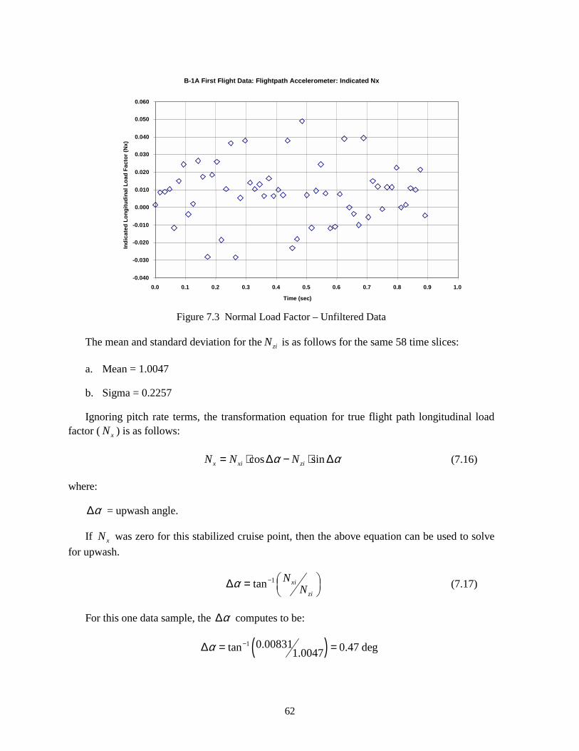
62

B-1A First Flight Data: Flightpath Accelerometer: Indicated Nx

-0.040

-0.030

-0.020

-0.010

0.000

0.010

0.020

0.030

0.040

0.050

0.060

0.0 0.1 0.2 0.3 0.4 0.5 0.6 0.7 0.8 0.9 1.0

Time (sec)

Indi

cate

d Lo

ngitu

dina

l Loa

d Fa

ctor

(Nx)

Figure 7.3 Normal Load Factor – Unfiltered Data

The mean and standard deviation for the ziN is as follows for the same 58 time slices:

a. Mean = 1.0047

b. Sigma = 0.2257

Ignoring pitch rate terms, the transformation equation for true flight path longitudinal load factor ( xN ) is as follows:

cos sinx xi ziN N Nα α= ⋅ ∆ − ⋅ ∆ (7.16)

where:

α∆ = upwash angle.

If xN was zero for this stabilized cruise point, then the above equation can be used to solve for upwash.

1tan xi

zi

NNα − ∆ =

(7.17)

For this one data sample, the α∆ computes to be:

( )1 0.00831tan 0.47 deg1.0047α −∆ = =

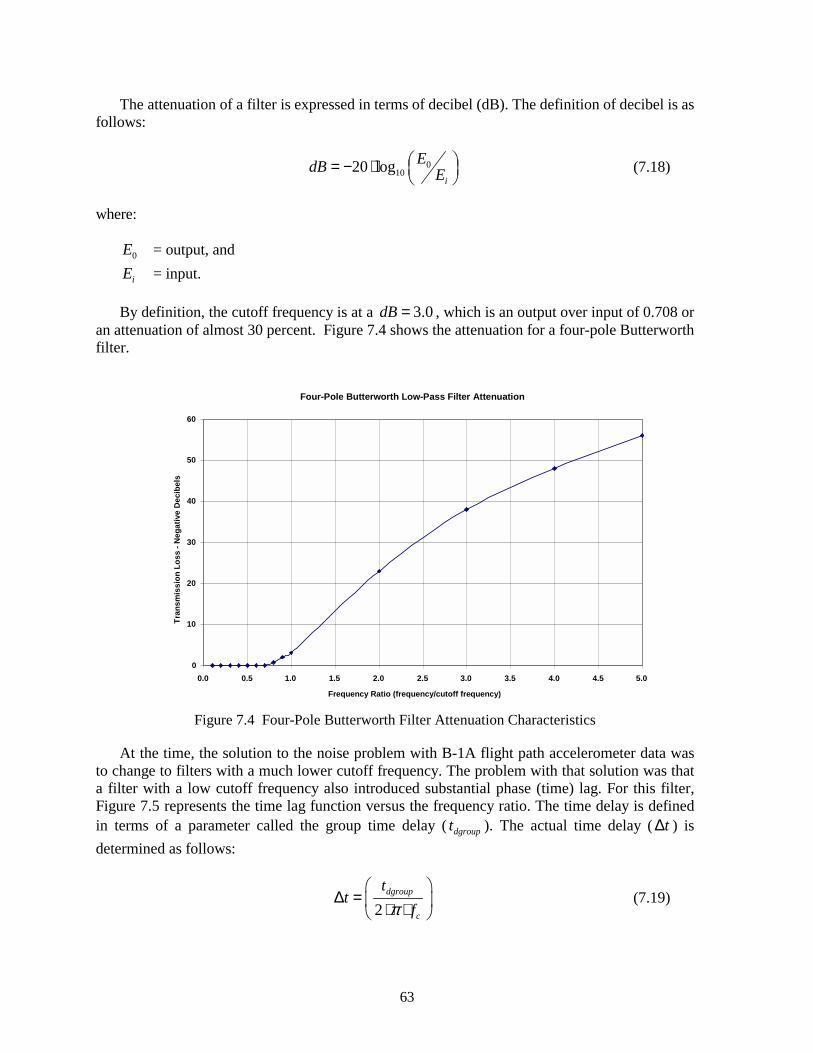
63

The attenuation of a filter is expressed in terms of decibel (dB). The definition of decibel is as follows:

01020 log

i

EdB E = − ⋅

(7.18)

where:

0E = output, and

iE = input.

By definition, the cutoff frequency is at a 3.0dB = , which is an output over input of 0.708 or an attenuation of almost 30 percent. Figure 7.4 shows the attenuation for a four-pole Butterworth filter.

Four-Pole Butterworth Low-Pass Filter Attenuation

0

10

20

30

40

50

60

0.0 0.5 1.0 1.5 2.0 2.5 3.0 3.5 4.0 4.5 5.0

Frequency Ratio (frequency/cutoff frequency)

Tran

smis

sion

Los

s - N

egat

ive

Dec

ibel

s

Figure 7.4 Four-Pole Butterworth Filter Attenuation Characteristics

At the time, the solution to the noise problem with B-1A flight path accelerometer data was to change to filters with a much lower cutoff frequency. The problem with that solution was that a filter with a low cutoff frequency also introduced substantial phase (time) lag. For this filter, Figure 7.5 represents the time lag function versus the frequency ratio. The time delay is defined in terms of a parameter called the group time delay ( dgroupt ). The actual time delay ( t∆ ) is determined as follows:

2

dgroup

c

tt

fπ

∆ = ⋅ ⋅ (7.19)

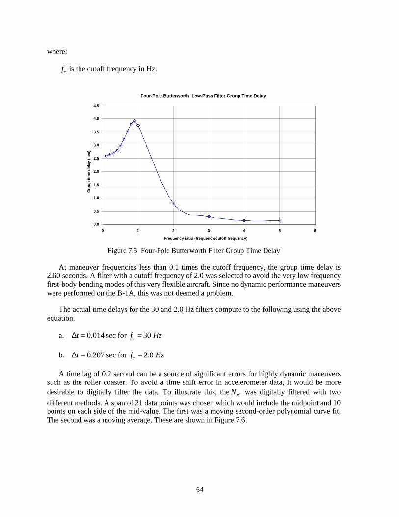
64

where:

cf is the cutoff frequency in Hz.

Four-Pole Butterworth Low-Pass Filter Group Time Delay

0.0

0.5

1.0

1.5

2.0

2.5

3.0

3.5

4.0

4.5

0 1 2 3 4 5 6

Frequency ratio (frequency/cutoff frequency)

Gro

up ti

me

dela

y (s

ec)

Figure 7.5 Four-Pole Butterworth Filter Group Time Delay

At maneuver frequencies less than 0.1 times the cutoff frequency, the group time delay is 2.60 seconds. A filter with a cutoff frequency of 2.0 was selected to avoid the very low frequency first-body bending modes of this very flexible aircraft. Since no dynamic performance maneuvers were performed on the B-1A, this was not deemed a problem.

The actual time delays for the 30 and 2.0 Hz filters compute to the following using the above equation.

a. 0.014 sec for 30ct f Hz∆ = =

b. 0.207 sec for 2.0ct f Hz∆ = =

A time lag of 0.2 second can be a source of significant errors for highly dynamic maneuvers such as the roller coaster. To avoid a time shift error in accelerometer data, it would be more desirable to digitally filter the data. To illustrate this, the xiN was digitally filtered with two different methods. A span of 21 data points was chosen which would include the midpoint and 10 points on each side of the mid-value. The first was a moving second-order polynomial curve fit. The second was a moving average. These are shown in Figure 7.6.

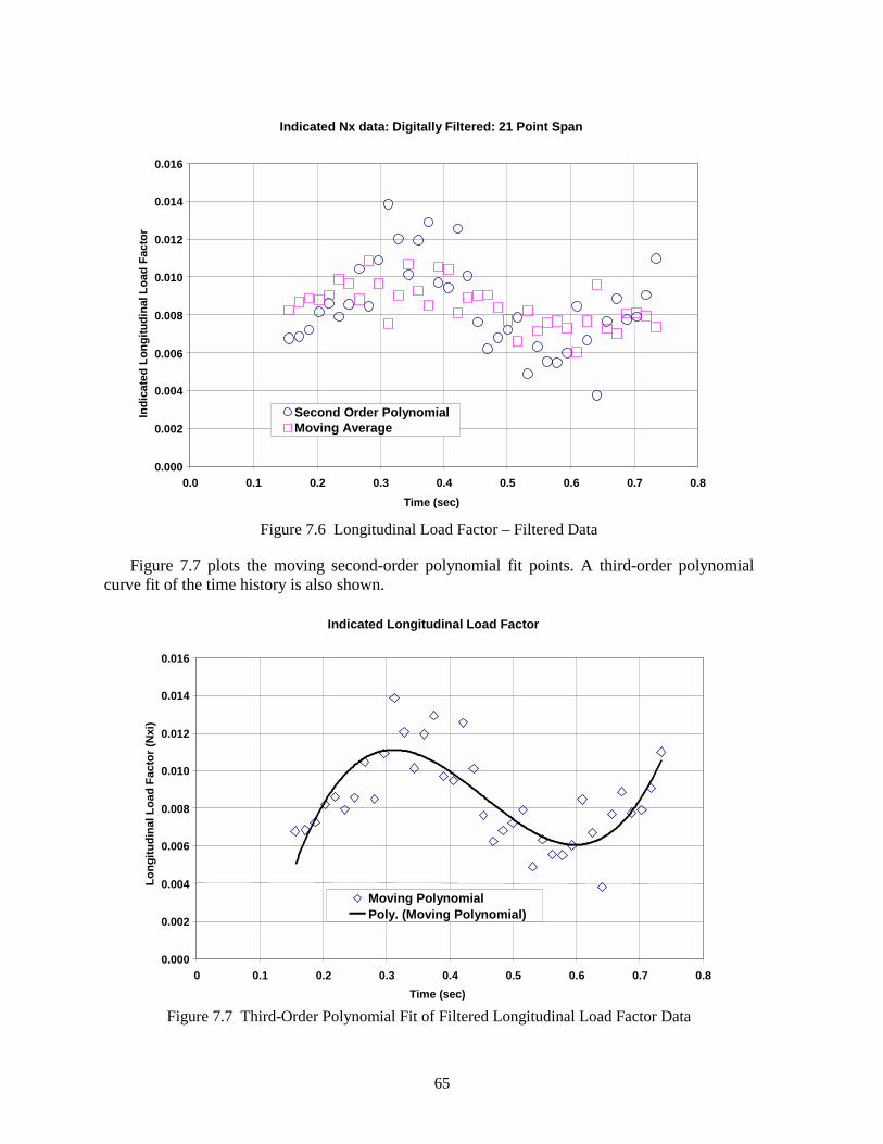
65

Indicated Nx data: Digitally Filtered: 21 Point Span

0.000

0.002

0.004

0.006

0.008

0.010

0.012

0.014

0.016

0.0 0.1 0.2 0.3 0.4 0.5 0.6 0.7 0.8Time (sec)

Indi

cate

d Lo

ngitu

dina

l Loa

d Fa

ctor

Second Order PolynomialMoving Average

Figure 7.6 Longitudinal Load Factor – Filtered Data

Figure 7.7 plots the moving second-order polynomial fit points. A third-order polynomial curve fit of the time history is also shown.

Indicated Longitudinal Load Factor

0.000

0.002

0.004

0.006

0.008

0.010

0.012

0.014

0.016

0 0.1 0.2 0.3 0.4 0.5 0.6 0.7 0.8Time (sec)

Long

itudi

nal L

oad

Fact

or (N

xi)

Moving PolynomialPoly. (Moving Polynomial)

Figure 7.7 Third-Order Polynomial Fit of Filtered Longitudinal Load Factor Data

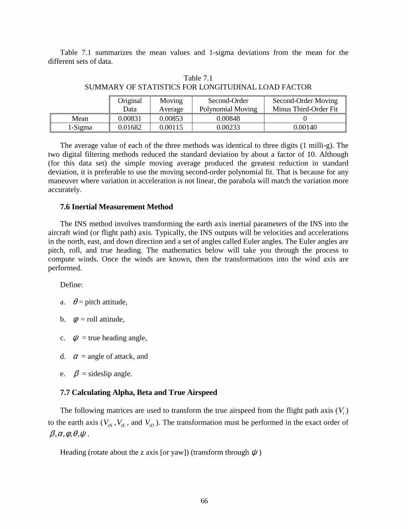
66

Table 7.1 summarizes the mean values and 1-sigma deviations from the mean for the different sets of data.

Table 7.1 SUMMARY OF STATISTICS FOR LONGITUDINAL LOAD FACTOR

Original Data

Moving Average

Second-Order Polynomial Moving

Second-Order Moving Minus Third-Order Fit

Mean 0.00831 0.00853 0.00848 0 1-Sigma 0.01682 0.00115 0.00233 0.00140

The average value of each of the three methods was identical to three digits (1 milli-g). The

two digital filtering methods reduced the standard deviation by about a factor of 10. Although (for this data set) the simple moving average produced the greatest reduction in standard deviation, it is preferable to use the moving second-order polynomial fit. That is because for any maneuver where variation in acceleration is not linear, the parabola will match the variation more accurately.

7.6 Inertial Measurement Method

The INS method involves transforming the earth axis inertial parameters of the INS into the aircraft wind (or flight path) axis. Typically, the INS outputs will be velocities and accelerations in the north, east, and down direction and a set of angles called Euler angles. The Euler angles are pitch, roll, and true heading. The mathematics below will take you through the process to compute winds. Once the winds are known, then the transformations into the wind axis are performed.

Define:

a. θ = pitch attitude,

b. φ = roll attitude,

c. ψ = true heading angle,

d. α = angle of attack, and

e. β = sideslip angle.

7.7 Calculating Alpha, Beta and True Airspeed

The following matrices are used to transform the true airspeed from the flight path axis ( tV ) to the earth axis ( tNV , tEV , and tDV ). The transformation must be performed in the exact order of

, , , ,β α φ θ ψ .

Heading (rotate about the z axis [or yaw]) (transform through ψ )

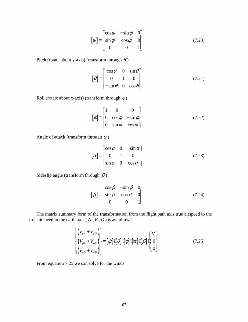
67

[ ]cos sin 0sin cos 0

0 0 1

ψ ψψ ψ ψ

− =

(7.20)

Pitch (rotate about y-axis) (transform through θ )

[ ]cos 0 sin

0 1 0sin 0 cos

θ θθ

θ θ

= −

(7.21)

Roll (rotate about x-axis) (transform through φ )

[ ]1 0 00 cos sin0 sin cos

φ φ φφ φ

= −

(7.22)

Angle of attack (transform through α )

[ ]cos 0 sin

0 1 0sin 0 cos

α αα

α α

− =

(7.23)

Sideslip angle (transform through β )

[ ]cos sin 0sin cos 0

0 0 1

β ββ β β

− =

(7.24)

The matrix summary form of the transformation from the flight path axis true airspeed to the true airspeed in the earth axis ( N , E , D ) is as follows:

( )( )( )

[ ] [ ] [ ] [ ] [ ] 00

gN wNt

gE wE

gD wD

V V VV V

V V

ψ θ φ α β

+ + = ⋅ ⋅ ⋅ ⋅ ⋅

+

(7.25)

From equation 7.25 we can solve for the winds.

68

[ ] [ ] [ ] [ ] [ ] 00

wN t gN

wE gE

wD gD

V V VV VV V

ψ θ φ α β = ⋅ ⋅ ⋅ ⋅ −

(7.26)

The equation above is the general matrix formula. During a typical wind calibration, we will assume the vertical wind ( wDV ), the sideslip angle ( β ), and the bank angle (φ) are equal to zero. Equation 7.26 represents three equations with at least five unknowns. The five unknowns are the three components of wind ( ),wN wE wDV V and V and α and β .

Then the α calculation reduces to the following:

α θ γ= − (7.27)

1sint

hVγ − = =

! flight path angle (7.28)

gDh V= − =! rate of climb (7.29)

We now wish to perform the reverse transformation; that is, to transform the components of true airspeed in the earth axis to the flight path. To transform the components, reverse the order of the matrix multiplication and take the transpose of each individual matrix. In this case, the transpose is the same as the inverse. To take the transpose of these unique matrices reverse all the off-diagonal terms and keep all the diagonal terms the same. For instance, the [ ]Tβ matrix derives from equation 7.24 as follows:

[ ]cos sin 0 cos sin 0sin cos 0 sin cos 0

0 0 1 0 0 1

T

Tβ β β β

β β β β β−

= = −

(7.30)

The matrix formula is as follows:

[ ] [ ] [ ] [ ] [ ] 00

tN tT T T T T

tE

tD

V VVV

β α φ θ ψ ⋅ ⋅ ⋅ ⋅ ⋅ =

(7.31)

We can calculate all the velocities in the equation 7.31 using the winds determined during the wind calibration (equation 7.26) as follows:

tN gN wNV V V= + (7.32)

tE gE wEV V V= + (7.33)

69

tD gD wDV V V= + (7.34)

( )2 2 2t tN tE tDV V V V= + + (7.35)

The airspeed components in the body axis ( , ,x y z ) are calculated in the following matrix manner:

[ ] [ ] [ ]bx tN

T T Tby tE

bz tD

V VV VV V

φ θ ψ = ⋅ ⋅ ⋅

(7.36)

Next, transform the body axis to the flight path axis through angle of attack and sideslip angle as follows:

[ ] [ ] 00

bx tT T

by

bz

V VVV

β α ⋅ ⋅ =

(7.37)

Expanding the alpha and beta transpose matrices and writing them out:

cos sin 0 cos 0 sinsin cos 0 0 1 0 00 0 1 sin 0 cos 0

bx t

by

bz

V VVV

β β α αβ β

α α

− ⋅ ⋅ = −

(7.38)

cos cos sin cos sinsin cos cos sin sin 0

sin 0 cos 0

bx t

by

bz

V VVV

β α β β αβ α β β α

α α

⋅ ⋅ − ⋅ − ⋅ ⋅ = −

(7.39)

Multiplying out the above matrix yields three equations from which we will derive formulas for α and β . When complete, these formulas should be the same as presented earlier. In the axis systems and equations of motion section, the angles were derived by geometry without the following matrix mathematics:

cos cos sin cos sinbx by bz tV V V Vβ α β β α⋅ ⋅ + ⋅ + ⋅ ⋅ = (7.40)

sin cos cos sin sin 0bx by bzV V Vβ α β β α− ⋅ ⋅ + ⋅ − ⋅ ⋅ = (7.41)

sin cos 0bx bzV Vα α− ⋅ + ⋅ = (7.42)

Equation 7.42 yields a formula for angle of attack.

70

sin / cos tan bz

bx

VVα α α= = (7.43)

1tan bz

bx

VVα − =

(7.44)

Inserting the result for bxV from equation 7.44 into equation 7.40:

cossinbx bzV Vα

α= ⋅

2 2cos sincos sin cos

sin sinbz by bz tV V V Vα αβ β βα α

⋅ ⋅ + ⋅ + ⋅ ⋅ = (7.45)

Collecting terms and using the trigonometric identity 2 2sin cos 1α α+ = :

cos sinsin

bzby t

V V Vβ βα

⋅ + ⋅ = (7.46)

Now, we will use equations 7.41 and 7.42 to substitute for the term in the square brackets. Replace bxV in 7.41 using 7.42.

2 2cos sinsin cos sin 0

sin sinbz by bzV V Vα αβ β βα α

− ⋅ ⋅ + ⋅ − ⋅ ⋅ =

( )2 2cos sin

sin cos 0sin bz byV Vα α

β βα

+ − ⋅ ⋅ + ⋅ =

cossin sin

bzby

V Vβα β

= ⋅ (7.47)

Finally, substituting equation 7.47 into equation 7.46:

2cos sincos

sin sinby by tV V Vβ βββ β

⋅ ⋅ + ⋅ =

sinby

tV Vβ =

1sin by

t

VVβ − =

(7.48)

Compare equations 7.44 and 7.48 to equations 2.11 and 2.12.

We now wish to perform the reverse transformation; that is, to transform the components of true airspeed in the Earth axis to the flight path. To transform the components, reverse the order

71

of the matrix multiplication and take the transpose of each individual matrix. The matrix formula is as follows:

[ ] [ ] [ ] [ ] [ ] 00

tN tT T T T T

tE

tD

V VVV

β α φ θ ψ ⋅ ⋅ ⋅ ⋅ ⋅ =

(7.49)

We can readily solve for the true airspeed components from the above.

The airspeed components in the body axis ( , ,x y z ) are calculated in the following matrix manner:

[ ] [ ] [ ]bx tN

T T Tby tE

bz tD

V VV VV V

φ θ ψ = ⋅ ⋅ ⋅

(7.50)

From true airspeed and the body axis true airspeed components, angle of attack and sideslip are computed using equations 7.44 and 7.48. The α and β are required in order to transform the earth axis accelerations to the flight path axis.

7.8 Flight Path Accelerations

To compute the accelerations in the flight path requires first computing the accelerations in the N, E, and D axis. Even when the accelerations are available as a direct output of an INS, it is desirable to compute the accelerations by taking numerical derivatives of the inertial velocities. This is because the accelerations are sensing the high frequency vibrations of the aircraft and are usually quite noisy. The typical INS updates at 50 samples per second. If one simply samples the velocity data at no more than about 5 samples per second and then takes a derivative, the noise will be dramatically reduced. The acceleration formulas are as follows:

( ) ( )

( )2

gN gNN

V t t V t tA t

t+ ∆ − −∆

=⋅∆

(7.51)

( ) ( )

( )2

gE gEE

V t t V t tA t

t+ ∆ − −∆

=⋅∆

(7.52)

0

( ) ( )( )

2gD gD

D

V t t V t tA t g

t+ ∆ − −∆

= −⋅∆

(7.53)

The velocities in the equations 7.51 through 7.53 are the inertial (or ground) speeds, not the airspeeds. We are computing inertial accelerations in the N, E, and D axis. However, we will later transform these into the wind axis. They are still inertial accelerations, but the components in our wind axis system. Note that the down (or z ) component involves subtracting out a gravity term. Since the vertical component of acceleration is down, we are actually adding in a gravity

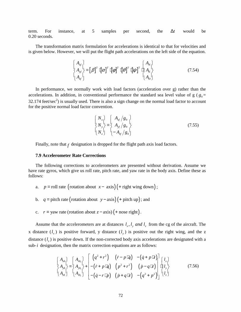
72

term. For instance, at 5 samples per second, the t∆ would be 0.20 seconds.

The transformation matrix formulation for accelerations is identical to that for velocities and is given below. However, we will put the flight path accelerations on the left side of the equation.

[ ] [ ] [ ] [ ] [ ]xf N

T T T T Tyf E

zf D

A AA AA A

β α φ θ ψ = ⋅ ⋅ ⋅ ⋅ ⋅

(7.54)

In performance, we normally work with load factors (acceleration over g) rather than the accelerations. In addition, in conventional performance the standard sea level value of g ( 0g = 32.174 feet/sec2) is usually used. There is also a sign change on the normal load factor to account for the positive normal load factor convention.

0

0

0

x xf

y yf

z zf

N A gN A gN A g

=

−

(7.55)

Finally, note that f designation is dropped for the flight path axis load factors.

7.9 Accelerometer Rate Corrections

The following corrections to accelerometers are presented without derivation. Assume we have rate gyros, which give us roll rate, pitch rate, and yaw rate in the body axis. Define these as follows:

a. ( ) ( )roll rate rotation about axis right wing downp x= − + ;

b. ( ) ( )pitch rate rotation about axis pitch upq y= − + ; and

c. ( )yaw rate (rotation about axis) nose rightr z= − + .

Assume that the accelerometers are at distances ,x y zl l and l from the cg of the aircraft. The x distance ( xl ) is positive forward, y distance ( yl ) is positive out the right wing, and the z

distance ( zl ) is positive down. If the non-corrected body axis accelerations are designated with a sub- i designation, then the matrix correction equations are as follows:

( ) ( ) ( )( ) ( ) ( )( ) ( ) ( )

2 2

2 2

2 2

i

i

i

xb xb x

yb yb y

zb zb z

q r r p q q p rA A lA A r p q p r p q r lA A lq r p p q r q p

+ − ⋅ − + ⋅ = + − + ⋅ + − ⋅ ⋅ − − ⋅ + ⋅ − +

! !

! !

! !

(7.56)

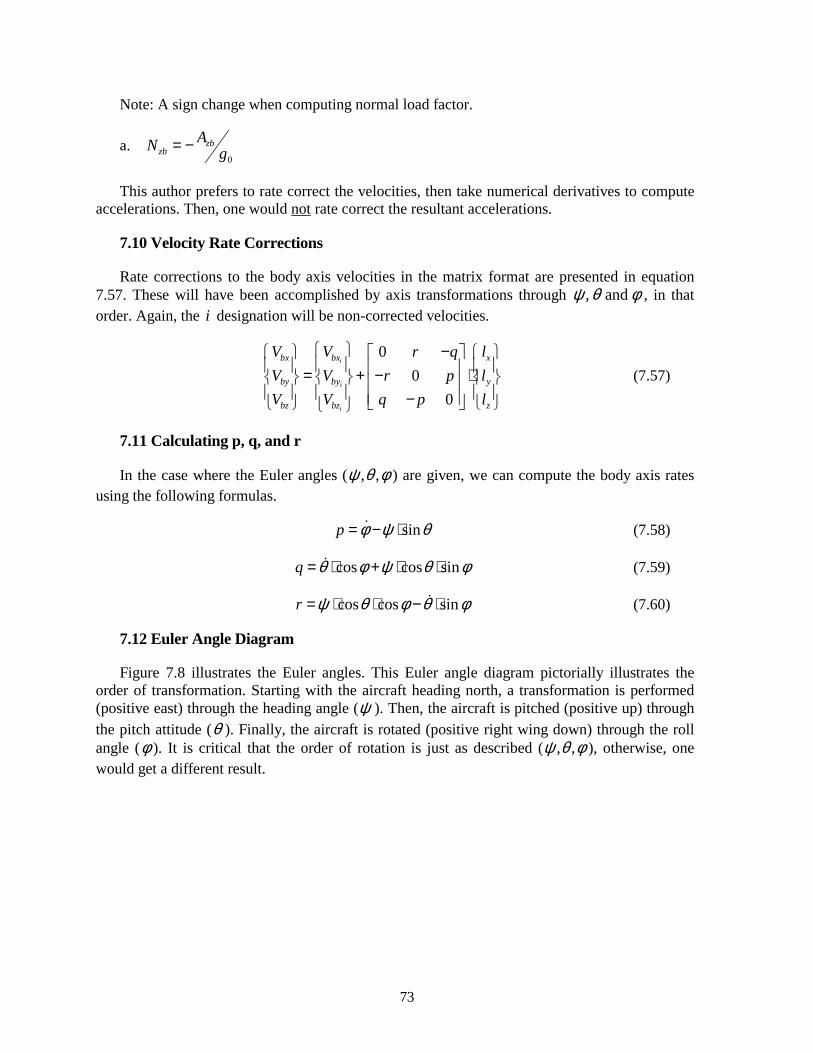
73

Note: A sign change when computing normal load factor.

a. 0

zbzb

AN g= −

This author prefers to rate correct the velocities, then take numerical derivatives to compute accelerations. Then, one would not rate correct the resultant accelerations.

7.10 Velocity Rate Corrections

Rate corrections to the body axis velocities in the matrix format are presented in equation 7.57. These will have been accomplished by axis transformations through , andψ θ φ , in that order. Again, the i designation will be non-corrected velocities.

0

00

i

i

i

bx bx x

by by y

bz bz z

V V r q lV V r p lV V q p l

− = + − ⋅

−

(7.57)

7.11 Calculating p, q, and r

In the case where the Euler angles ( , ,ψ θ φ ) are given, we can compute the body axis rates using the following formulas.

sinp φ ψ θ= − ⋅! ! (7.58)

cos cos sinq θ φ ψ θ φ= ⋅ + ⋅ ⋅! ! (7.59)

cos cos sinr ψ θ φ θ φ= ⋅ ⋅ − ⋅!! (7.60)

7.12 Euler Angle Diagram

Figure 7.8 illustrates the Euler angles. This Euler angle diagram pictorially illustrates the order of transformation. Starting with the aircraft heading north, a transformation is performed (positive east) through the heading angle (ψ ). Then, the aircraft is pitched (positive up) through the pitch attitude (θ ). Finally, the aircraft is rotated (positive right wing down) through the roll angle (φ ). It is critical that the order of rotation is just as described ( , ,ψ θ φ ), otherwise, one would get a different result.

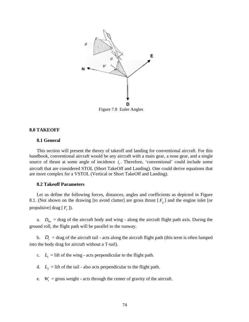
74

Figure 7.8 Euler Angles

8.0 TAKEOFF

8.1 General

This section will present the theory of takeoff and landing for conventional aircraft. For this handbook, conventional aircraft would be any aircraft with a main gear, a nose gear, and a single source of thrust at some angle of incidence ti . Therefore, ‘conventional’ could include some aircraft that are considered STOL (Short TakeOff and Landing). One could derive equations that are more complex for a VSTOL (Vertical or Short TakeOff and Landing).

8.2 Takeoff Parameters

Let us define the following forces, distances, angles and coefficients as depicted in Figure 8.1. (Not shown on the drawing [to avoid clutter] are gross thrust [ gF ] and the engine inlet [or propulsive] drag [ eF ]).

a. bwD = drag of the aircraft body and wing - along the aircraft flight path axis. During the ground roll, the flight path will be parallel to the runway.

b. tD = drag of the aircraft tail - acts along the aircraft flight path (this term is often lumped into the body drag for aircraft without a T-tail).

c. 1L = lift of the wing - acts perpendicular to the flight path.

d. 2L = lift of the tail - also acts perpendicular to the flight path.

e. tW = gross weight - acts through the center of gravity of the aircraft.

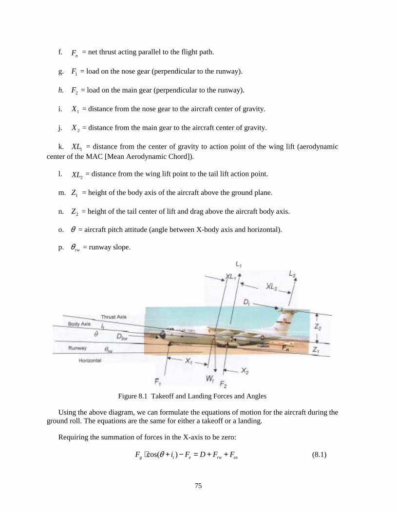
75

f. nF = net thrust acting parallel to the flight path.

g. 1F = load on the nose gear (perpendicular to the runway).

h. 2F = load on the main gear (perpendicular to the runway).

i. 1X = distance from the nose gear to the aircraft center of gravity.

j. 2X = distance from the main gear to the aircraft center of gravity.

k. 1XL = distance from the center of gravity to action point of the wing lift (aerodynamic center of the MAC [Mean Aerodynamic Chord]).

l. 2XL = distance from the wing lift point to the tail lift action point.

m. 1Z = height of the body axis of the aircraft above the ground plane.

n. 2Z = height of the tail center of lift and drag above the aircraft body axis.

o. θ = aircraft pitch attitude (angle between X-body axis and horizontal).

p. rwθ = runway slope.

Figure 8.1 Takeoff and Landing Forces and Angles

Using the above diagram, we can formulate the equations of motion for the aircraft during the ground roll. The equations are the same for either a takeoff or a landing.

Requiring the summation of forces in the X-axis to be zero:

cos( )g t e rw exF i F D F Fθ⋅ + − = + + (8.1)

76

where:

D = total aerodynamic drag,

rwF = total runway resistance = runway friction plus runway slope effect, and

exF = excess thrust (positive forward).

bw tD D D= + (8.2)

1 1 2 2 sin( )rw t rwF F F Wµ µ θ= ⋅ + ⋅ + ⋅ (8.3)

where:

1µ = coefficient of friction associated with the nosewheels, and

2µ = coefficient of friction associated with the main wheels.

ex x tF N W= ⋅ (positive forward) (8.4)

where:

xN = longitudinal load factor.

0/x xN A g= (8.5)

x gA V= ! (8.6)

where:

gV = groundspeed.

Note that the longitudinal load factor definition on the ground includes only the velocity derivative term. In the air, the gravity component is included. On the ground, we will account for the gravity component in the sin( )t rwW θ⋅ term.

Collecting terms:

1 1 2 2cos( ) ( ) ( sin( ))g t e bw t t rw exF i F D D F F W Fθ µ µ θ⋅ + − = + + ⋅ + ⋅ + ⋅ + (8.7)

Requiring the summation of forces in the Z-axis to be zero:

1 2 1 2 cos( )t rwL L F F W θ+ + + = ⋅ (8.8)

Require the summation of moments about the Y-axis to be zero. Take moments about the main wheels, since the aircraft will pitch about the main wheels during the takeoff or landing ground roll. Ignore any pitch dynamics during the ground roll or any moment caused by the vertical component of gross thrust.

77

( ) ( ) ( )1 1 2 1 2 1 1 1 2 1sin( )bw t t rwF X X L X XL D Z D Z Z W Zθ⋅ + + ⋅ − + ⋅ + ⋅ + + ⋅ ⋅ =

( ) ( )2 1 2 1 2 2cos( ) cos( )t rw g t eW X F i F Z L XL XL Xθ⋅ ⋅ + ⋅ − ⋅ + ⋅ + − (8.9)

What we now have is three equations with three unknowns for purposes of simulating a takeoff or landing ground roll. It is assumed that one has a thrust and drag model for the lift, drag, gross thrust, and propulsive drag terms in the above equations. However, the lift and drag models may not be for in-ground effect. If no in-ground effect corrections are available, then some empirical predictions can be used until flight test results are available to create an in-ground effect model.

The three unknowns are the two normal forces on the wheels ( 1F and 2F ) and the excess thrust ( exF ). The primary parameter of interest is the excess thrust from which we can compute the derivative of groundspeed. Once we have the excess thrust, we can integrate the groundspeed derivative to obtain speed and distance versus time.

Collecting equations 8.7 through 8.9:

1 1 2 2cos( ) sin( )g t e bw t t rw exF i F D D F F W Fθ µ µ θ⋅ + − = + + ⋅ + ⋅ + ⋅ +

1 2 1 2 cos( )t rwL L F F W θ+ + + = ⋅

( ) ( ) ( ) ( )1 1 2 1 2 1 1 2 1sint t rwF X X L X XL D Z Z W Zθ⋅ + + ⋅ − + ⋅ + + ⋅ ⋅ =

( ) ( )2 1 2 1 2 2cos( ) cos( )t rw g t eW X F i F Z L XL XL Xθ⋅ ⋅ + ⋅ − ⋅ + ⋅ + −

Rearranging the equations:

1 1 2 2 cos( ) sin( )ex g t e bw t t rwF F F F i F D D Wµ µ θ + ⋅ + ⋅ = ⋅ − − − − ⋅ (8.10)

[ ]1 2 1 2cos( )t rwF F W L Lθ+ = ⋅ − − (8.11)

( )1 2 1X X F+ ⋅ =

( ) ( )( ) ( )

2 1 1 2 1 2 2

1 2 1 1 2

cos( ) sin( ) cos( )t rw t rw g t e

t

W X W Z F i F Z L XL XL X

L X XL D Z Z

θ θ θ ⋅ ⋅ − ⋅ ⋅ + ⋅ + − ⋅ + ⋅ + − − ⋅ − − ⋅ +

(8.12)

We will define the terms in the square brackets in 8.10 through 8.12 as 1A , 2A , and 3A .

Then we can rewrite equations 8.10 through 8.12 in three by three-matrix form as follows:

( )

1 2 1

1 2

1 2 2 3

10 1 10 0

exF AF A

X X F A

µ µ ⋅ = +

(8.13)

78

During the course of flight test, we measure excess thrust ( exF ). However, the thrust and drag may be unknown, or at least not known precisely. Therefore, we may need to iterate between the above equation and the solution of the above equation. The 1A term is thrust minus drag minus the runway component of weight.

The matrix relationship in equation 8.13 can be solved by multiplying both sides by the inverse of the square matrix.

( )

11 2 1

1 2

2 1 2 3

10 1 10 0

exF AF AF X X A

µ µ−

= ⋅ +

(8.14)

8.3 Developing a Takeoff Simulation

Usually, the contractor will provide an initial estimated model for lift and drag as a function of angle of attack (α ). As mentioned before, one may need to supplement this model with empirical ground effect estimation, such as that found in the NASA takeoff and landing simulation program listed in the Bibliography. During the ground roll, the angle of attack is equal to the pitch attitude (α θ= ). The thrust incidence angle is usually zero or small.

Only the most precise simulations will typically account for a separate tail and body drag, so we can ignore tD in many cases. Accounting for tail lift and drag becomes more important for modeling braking performance to determine the load distribution on the main gear and the nose gear. For takeoff performance, a value of 0.015 is usually assumed for the rolling coefficient of friction (µ ). Values of µ for a dry runway up to 0.025 are also used. In addition, a point mass model will be assumed with all the forces acting through the cg of the aircraft. Further, since

g eF F>> at low airspeeds, we make the following approximation:

( ) cos( )n g e tF F F iθ≅ − ⋅ + (8.15)

sin( )ex n t rwF F F D Wµ θ+ ⋅ = − − ⋅ (8.16)

cos( )t rwF W Lθ= ⋅ − (8.17)

where:

F =main gear load (assume all load on the main gear).

Combining equations 8.16 and 8.17:

( )cos( ) sin( )ex t rw n t rwF W L F D Wµ θ θ+ ⋅ ⋅ − = − − ⋅ (8.18)

79

Equation 8.18 can be used in two ways. First, to solve excess thrust (equation 8.19). Second, to solve thrust minus drag (equation 8.20). We know (or assume values for) the other variables: gross weight, runway slope, rolling friction, and aerodynamic lift.

[ ] ( )sin( ) cos( )ex n t rw t rwF F D W W Lθ µ θ= − − ⋅ − ⋅ ⋅ − (8.19)

[ ] ( )sin( ) cos( )n ex t rw t rwF D F W W Lθ µ θ− = + ⋅ + ⋅ ⋅ − (8.20)

From equation 8.19, we can compute the excess thrust during the ground roll of the aircraft. One would be provided models for net thrust drag and lift. The drag and lift models would be in the form of drag and lift coefficients versus angle of attack. Typical model formulations are as follows:

( ), ,n CF f M H T= (8.21)

( ),L AGLC f hα= (8.22)

( ),D L AGLC f C h= (8.23)

where:

M = Mach number, CH = pressure altitude (subscript C denotes calibrated),

T = ambient temperature, and AGLh = aircraft wing height above ground level.

The parameter AGLh is needed to account for ground effect. The above are just typical model forms. They may also include Reynolds number (or skin friction drag) terms in the drag polar. In addition, the engine is usually not at 100-percent thrust at brake release so a thrust spool up factor needs to be supplied. One would also incorporate a fuel flow model to compute fuel used during takeoff. This is to account for the fuel used for mission calculations.

8.4 Ground Effect

Figure 8.2 is typical of a relationship defining the decrease in drag due to lift in-ground effect. The data points were taken from a curve found in two separate textbooks, neither of which gave a source for the data. The texts are The Illustrated Guide to Aerodynamics by H.C. Smith and Technical Aerodynamics by Karl D. Wood. The suspicion is that this is from some early NACA work. The equation is a curve fit of the points.

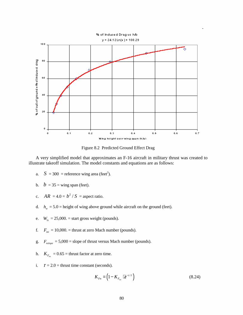
80

Figure 8.2 Predicted Ground Effect Drag

A very simplified model that approximates an F-16 aircraft in military thrust was created to illustrate takeoff simulation. The model constants and equations are as follows:

a. S = 300 = reference wing area (feet2).

b. b = 35 = wing span (feet).

c. AR = 4.0 = 2 /b S = aspect ratio.

d. wh = 5.0 = height of wing above ground while aircraft on the ground (feet).

e. tsW = 25,000. = start gross weight (pounds).

f. noF = 10,000. = thrust at zero Mach number (pounds).

g. nslopeF = 5,000 = slope of thrust versus Mach number (pounds).

h. noFK = 0.65 = thrust factor at zero time.

i. τ = 2.0 = thrust time constant (seconds).

( )/1no

tFn FK K e τ−= − ⋅ (8.24)

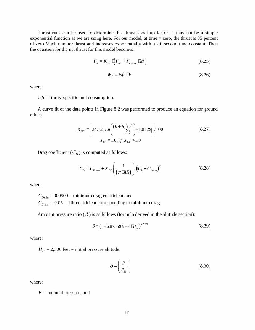
81

Thrust runs can be used to determine this thrust spool up factor. It may not be a simple exponential function as we are using here. For our model, at time = zero, the thrust is 35 percent of zero Mach number thrust and increases exponentially with a 2.0 second time constant. Then the equation for the net thrust for this model becomes:

( )n Fn no nslopeF K F F M= ⋅ + ⋅ (8.25)

f nW tsfc F= ⋅ (8.26)

where:

tsfc = thrust specific fuel consumption.

A curve fit of the data points in Figure 8.2 was performed to produce an equation for ground effect.

( )24.12 108.29 /100wGE

h hX Ln b += ⋅ +

(8.27)

1.0 , 1.0GE GEX if X= >

Drag coefficient ( DC ) is computed as follows:

( ) ( )2

min min1

D D GE L LC C X C CARπ

= + ⋅ − ⋅

(8.28)

where:

minDC = 0.0500 = minimum drag coefficient, and

minLC = 0.05 = lift coefficient corresponding to minimum drag.

Ambient pressure ratio (δ ) is as follows (formula derived in the altitude section):

( )5.25591 6.87559 6 CE Hδ = − − ⋅ (8.29)

where:

CH = 2,300 feet = initial pressure altitude.

SL

PP

δ

=

(8.30)

where:

P = ambient pressure, and

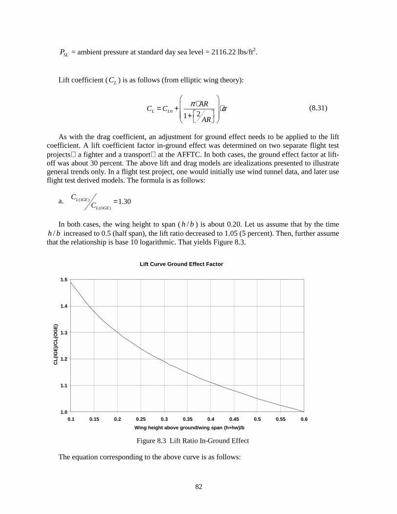
82

SLP = ambient pressure at standard day sea level = 2116.22 lbs/ft2.

Lift coefficient ( LC ) is as follows (from elliptic wing theory):

0 21L L

ARC CAR

π α ⋅ = + ⋅ +

(8.31)

As with the drag coefficient, an adjustment for ground effect needs to be applied to the lift coefficient. A lift coefficient factor in-ground effect was determined on two separate flight test projects a fighter and a transport at the AFFTC. In both cases, the ground effect factor at lift-off was about 30 percent. The above lift and drag models are idealizations presented to illustrate general trends only. In a flight test project, one would initially use wind tunnel data, and later use flight test derived models. The formula is as follows:

a. ( )

( )1.30L IGE

L OGE

CC =

In both cases, the wing height to span ( /h b ) is about 0.20. Let us assume that by the time /h b increased to 0.5 (half span), the lift ratio decreased to 1.05 (5 percent). Then, further assume

that the relationship is base 10 logarithmic. That yields Figure 8.3.

Lift Curve Ground Effect Factor

1.0

1.1

1.2

1.3

1.4

1.5

0.1 0.15 0.2 0.25 0.3 0.35 0.4 0.45 0.5 0.55 0.6Wing height above ground/wing span (h+hw)/b

CL(

IGE)

/CL(

OG

E)

Figure 8.3 Lift Ratio In-Ground Effect

The equation corresponding to the above curve is as follows:

83

( )( )( )10

( )0.8609 0.6282L IGE

wL OGE

C Log h h bC = − ⋅ + (8.32)

With the following constraint:

a. ( )

( )1.0L IGE

L OGE

CC ≥

The angle of attack is held to zero during the ground roll until a rotation speed is reached. This rotation speed (in this simulation example) is at a calibrated airspeed of 100 knots. Calibrated airspeed is normally displayed in the cockpit and was discussed in detail in Section 4.0 Airspeed. As will be shown in the later vectored thrust takeoff section, the selection of 100 knots as the rotation speed is probably much too low for an actual F-16. Upon reaching the rotation speed, the typical takeoff will rotate to some given angle of attack. Then, that angle of attack is held until the aircraft generates enough lift such that lift is greater than weight and the aircraft lifts off the runway. The angle-of-attack profile used in this example computer simulation is as follows:

( )last ttαα α ∆= + ⋅∆∆ (8.33)

where:

( ) 3.0tα∆ =∆ deg/sec.

The angle of attack (α ) is limited to a predetermined value. In this example simulation that value is 13 degrees. In the numerical integration, 13 degrees α is reached at 130 knots calibrated airspeed. The lift first exceeds weight at an airspeed of 132 knots. The aircraft (or the simulated aircraft) will lift off the ground when lift is greater than weight.

Lift and drag (formulas in lift and drag section) are computed as follows:

2 / 0.000675LL C M Sδ= ⋅ ⋅ ⋅ (8.34)

2 / 0.000675DD C M Sδ= ⋅ ⋅ ⋅ (8.35)

Finally, the last terms in our model are the runway resistance. We will assume zero runway slope.

µ = 0.015 rolling coefficient of friction.

Then,

( )rw tF W Lµ= ⋅ − (8.36) 0.0rw tF if L W= >

Combining terms:

84

( )ex n rwF F D F= − + (8.37)

ex x tF N W= ⋅ (8.38)

0

gx

t

V hN g V= +! ! (8.39)

During the ground roll, the h-dot ( h! ) term is zero. During the air phase, the normal load factor equation is used. Equation 8.40 is derived in the section on normal load factor during a climb.

0

cos( ) tz

VNgγγ ⋅= +!

(8.40)

1sint

hVγ − =

! flight path angle (8.41)

From the ,x zN N , and γ equations (8.39 through 8.41), we can numerically integrate groundspeed ( gV ) and geometric height ( h ). All of the forces, however, are functions of airspeed and pressure altitude. We have assumed a standard atmosphere for temperature. Standard atmosphere is defined in the altitude section.

288.15 (1.9812 /1000) CT H= − ⋅ (8.42)

t g wV V V= + (8.43)

where:

tV = true airspeed, and

wV = windspeed. We will assume windspeed equals zero.

The following equations were derived in Section 4.0 Airspeed.

/tM V a= (8.44)

SLa a θ= ⋅ = speed of sound (8.45)

where:

661.48SLa = knots.

( )288.15Tθ = = temperature ratio (8.46)

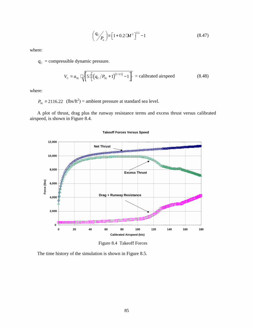
85

3.521 0.2 1C

a

q MP = + ⋅ −

(8.47)

where:

Cq = compressible dynamic pressure.

( )( ){ }1/3.55 1 1C SL C SLV a q P = ⋅ ⋅ + − = calibrated airspeed (8.48)

where:

2116.22SLP = (lbs/ft2) = ambient pressure at standard sea level.

A plot of thrust, drag plus the runway resistance terms and excess thrust versus calibrated airspeed, is shown in Figure 8.4.

Takeoff Forces Versus Speed

0

2,000

4,000

6,000

8,000

10,000

12,000

0 20 40 60 80 100 120 140 160 180

Calibrated Airspeed (kts)

Forc

e (lb

s)

Drag + Runway Resistance

Excess Thrust

Net Thrust

Figure 8.4 Takeoff Forces

The time history of the simulation is shown in Figure 8.5.

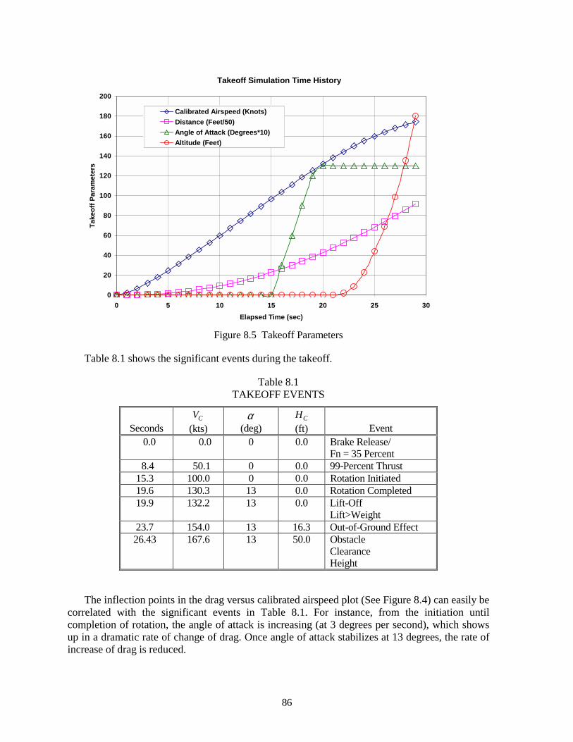
86

Takeoff Simulation Time History

0

20

40

60

80

100

120

140

160

180

200

0 5 10 15 20 25 30Elapsed Time (sec)

Take

off P

aram

eter

s

Calibrated Airspeed (Knots)Distance (Feet/50)Angle of Attack (Degrees*10)Altitude (Feet)

Figure 8.5 Takeoff Parameters

Table 8.1 shows the significant events during the takeoff.

Table 8.1 TAKEOFF EVENTS

Seconds

CV (kts)

α (deg)

CH (ft)

Event

0.0 0.0 0 0.0 Brake Release/ Fn = 35 Percent

8.4 50.1 0 0.0 99-Percent Thrust 15.3 100.0 0 0.0 Rotation Initiated 19.6 130.3 13 0.0 Rotation Completed 19.9 132.2 13 0.0 Lift-Off

Lift>Weight 23.7 154.0 13 16.3 Out-of-Ground Effect 26.43 167.6 13 50.0 Obstacle

Clearance Height

The inflection points in the drag versus calibrated airspeed plot (See Figure 8.4) can easily be correlated with the significant events in Table 8.1. For instance, from the initiation until completion of rotation, the angle of attack is increasing (at 3 degrees per second), which shows up in a dramatic rate of change of drag. Once angle of attack stabilizes at 13 degrees, the rate of increase of drag is reduced.

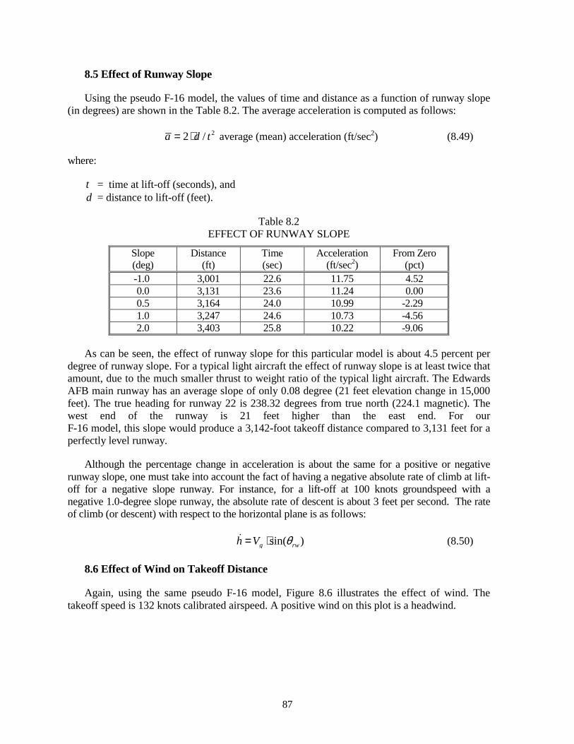
87

8.5 Effect of Runway Slope

Using the pseudo F-16 model, the values of time and distance as a function of runway slope (in degrees) are shown in the Table 8.2. The average acceleration is computed as follows:

22 /a d t= ⋅ average (mean) acceleration (ft/sec2) (8.49)

where:

t = time at lift-off (seconds), and d = distance to lift-off (feet).

Table 8.2 EFFECT OF RUNWAY SLOPE

Slope (deg)

Distance (ft)

Time (sec)

Acceleration (ft/sec2)

From Zero (pct)

-1.0 3,001 22.6 11.75 4.52 0.0 3,131 23.6 11.24 0.00 0.5 3,164 24.0 10.99 -2.29 1.0 3,247 24.6 10.73 -4.56 2.0 3,403 25.8 10.22 -9.06

As can be seen, the effect of runway slope for this particular model is about 4.5 percent per

degree of runway slope. For a typical light aircraft the effect of runway slope is at least twice that amount, due to the much smaller thrust to weight ratio of the typical light aircraft. The Edwards AFB main runway has an average slope of only 0.08 degree (21 feet elevation change in 15,000 feet). The true heading for runway 22 is 238.32 degrees from true north (224.1 magnetic). The west end of the runway is 21 feet higher than the east end. For our F-16 model, this slope would produce a 3,142-foot takeoff distance compared to 3,131 feet for a perfectly level runway.

Although the percentage change in acceleration is about the same for a positive or negative runway slope, one must take into account the fact of having a negative absolute rate of climb at lift-off for a negative slope runway. For instance, for a lift-off at 100 knots groundspeed with a negative 1.0-degree slope runway, the absolute rate of descent is about 3 feet per second. The rate of climb (or descent) with respect to the horizontal plane is as follows:

sin( )g rwh V θ= ⋅! (8.50)

8.6 Effect of Wind on Takeoff Distance

Again, using the same pseudo F-16 model, Figure 8.6 illustrates the effect of wind. The takeoff speed is 132 knots calibrated airspeed. A positive wind on this plot is a headwind.

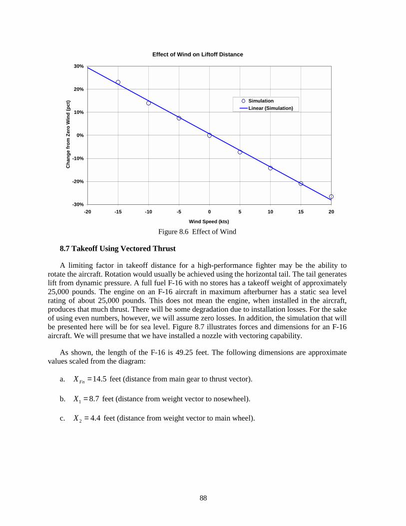
88

Effect of Wind on Liftoff Distance

-30%

-20%

-10%

0%

10%

20%

30%

-20 -15 -10 -5 0 5 10 15 20

Wind Speed (kts)

Cha

nge

from

Zer

o W

ind

(pct

) SimulationLinear (Simulation)

Figure 8.6 Effect of Wind

8.7 Takeoff Using Vectored Thrust

A limiting factor in takeoff distance for a high-performance fighter may be the ability to rotate the aircraft. Rotation would usually be achieved using the horizontal tail. The tail generates lift from dynamic pressure. A full fuel F-16 with no stores has a takeoff weight of approximately 25,000 pounds. The engine on an F-16 aircraft in maximum afterburner has a static sea level rating of about 25,000 pounds. This does not mean the engine, when installed in the aircraft, produces that much thrust. There will be some degradation due to installation losses. For the sake of using even numbers, however, we will assume zero losses. In addition, the simulation that will be presented here will be for sea level. Figure 8.7 illustrates forces and dimensions for an F-16 aircraft. We will presume that we have installed a nozzle with vectoring capability.

As shown, the length of the F-16 is 49.25 feet. The following dimensions are approximate values scaled from the diagram:

a. 14.5FnX = feet (distance from main gear to thrust vector).

b. 1 8.7X = feet (distance from weight vector to nosewheel).

c. 2 4.4X = feet (distance from weight vector to main wheel).

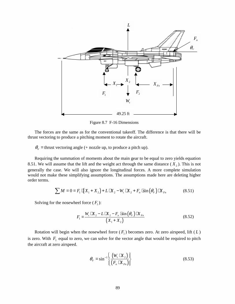
1X

Figure 8.7 F-1

The forces are the same as for the conventiothrust vectoring to produce a pitching moment to

Vθ = thrust vectoring angle (+ nozzle up, to p

Requiring the summation of moments about 8.51. We will assume that the lift and the weightgenerally the case. We will also ignore the lonwould not make these simplifying assumptions. order terms.

( )1 1 2 20M F X X L X= = ⋅ + + ⋅∑

Solving for the nosewheel force ( 1F ):

(

2 21

1

tW X L XF

X⋅ − ⋅ −

=+

Rotation will begin when the nosewheel forcis zero. With 1F equal to zero, we can solve for the aircraft at zero airspeed.

((

1sinVWF

θ − =

L

tW1F

2XFnX

V

nF

2F

49.25 ft

89

6 Dimensions

nal takeoff. The dif rotate the aircraft.

roduce a pitch up).

the main gear to be e act through the samgitudinal forces. AThe assumptions m

(2 sint nW X F− ⋅ + ⋅

( ))2

sinn V FnF XX

θ⋅ ⋅

e ( 1F ) becomes zerthe vector angle tha

))

2t

n Fn

XX

⋅ ⋅

ference is that there

qual to zero yields ee distance ( 2X ). Thi more complete simade here are deleting

)V FnXθ ⋅ (8.

(8.

o. At zero airspeed, lt would be required t

(8.

θ

will be

quation s is not ulation higher

51)

52)

ift ( L ) o pitch

53)

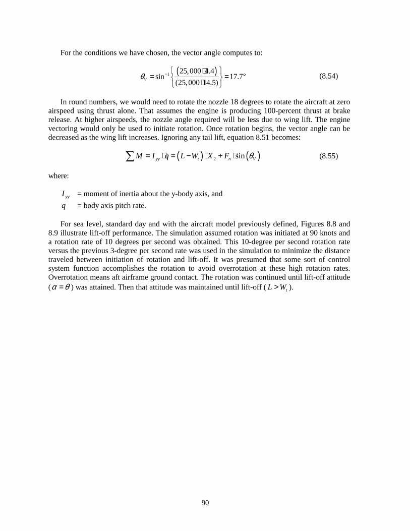
90

For the conditions we have chosen, the vector angle computes to:

( )1 25,000 4.4sin 17.7

(25,000 14.5)Vθ− ⋅

= = ° ⋅ (8.54)

In round numbers, we would need to rotate the nozzle 18 degrees to rotate the aircraft at zero airspeed using thrust alone. That assumes the engine is producing 100-percent thrust at brake release. At higher airspeeds, the nozzle angle required will be less due to wing lift. The engine vectoring would only be used to initiate rotation. Once rotation begins, the vector angle can be decreased as the wing lift increases. Ignoring any tail lift, equation 8.51 becomes:

( ) ( )2 sinyy t n VM I q L W X F θ= ⋅ = − ⋅ + ⋅∑ (8.55)

where:

yyI = moment of inertia about the y-body axis, and q = body axis pitch rate.

For sea level, standard day and with the aircraft model previously defined, Figures 8.8 and 8.9 illustrate lift-off performance. The simulation assumed rotation was initiated at 90 knots and a rotation rate of 10 degrees per second was obtained. This 10-degree per second rotation rate versus the previous 3-degree per second rate was used in the simulation to minimize the distance traveled between initiation of rotation and lift-off. It was presumed that some sort of control system function accomplishes the rotation to avoid overrotation at these high rotation rates. Overrotation means aft airframe ground contact. The rotation was continued until lift-off attitude (α θ= ) was attained. Then that attitude was maintained until lift-off ( tL W> ).

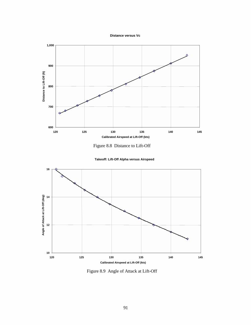
91

Distance versus Vc

600

700

800

900

1,000

120 125 130 135 140 145

Calibrated Airspeed at Lift-Off (kts)

Dis

tanc

e to

Lift

-Off

(ft)

Figure 8.8 Distance to Lift-Off

Takeoff: Lift-Off Alpha versus Airspeed

10

12

14

16

120 125 130 135 140 145


Ang

le o

f Atta

ck a

t Lift

-Off

(deg

)

Figure 8.9 Angle of Attack at Lift-Off

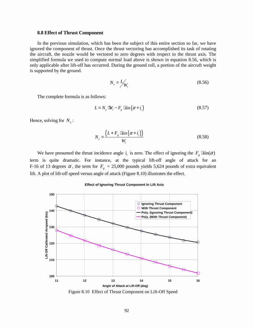
92

8.8 Effect of Thrust Component

In the previous simulation, which has been the subject of this entire section so far, we have ignored the component of thrust. Once the thrust vectoring has accomplished its task of rotating the aircraft, the nozzle would be vectored to zero degrees with respect to the thrust axis. The simplified formula we used to compute normal load above is shown in equation 8.56, which is only applicable after lift-off has occurred. During the ground roll, a portion of the aircraft weight is supported by the ground.

zt

LN W= (8.56)

The complete formula is as follows:

( )sinz t g tL N W F iα= ⋅ − ⋅ + (8.57)

Hence, solving for zN :

( )( )sing t

zt

L F iN

Wα+ ⋅ +

= (8.58)

We have presumed the thrust incidence angle ti is zero. The effect of ignoring the sin( )gF α⋅ term is quite dramatic. For instance, at the typical lift-off angle of attack for an F-16 of 13 degrees α , the term for gF = 25,000 pounds yields 5,624 pounds of extra equivalent lift. A plot of lift-off speed versus angle of attack (Figure 8.10) illustrates the effect.

Effect of Ignoring Thrust Component In Lift Axis

100

110

120

130

140

150

11 12 13 14 15 16Angle of Attack at Lift-Off (deg)

Lift-

Off

Cal

ibra

ted

Airs

peed

(kts

)

Ignoring Thrust ComponentWith Thrust ComponentPoly. (Ignoring Thrust Component)Poly. (With Thrust Component)

Figure 8.10 Effect of Thrust Component on Lift-Off Speed

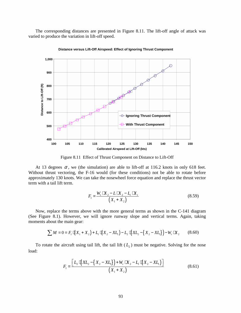
93

The corresponding distances are presented in Figure 8.11. The lift-off angle of attack was varied to produce the variation in lift-off speed.

Distance versus Lift-Off Airspeed: Effect of Ignoring Thrust Component

400

500

600

700

800

900

1,000

100 105 110 115 120 125 130 135 140 145 150Calibrated Airspeed at Lift-Off (kts)

Dis

tanc

e to

Lift

-Off

(ft)

Ignoring Thrust Component

With Thrust Component

Figure 8.11 Effect of Thrust Component on Distance to Lift-Off

At 13 degrees α , we (the simulation) are able to lift-off at 116.2 knots in only 618 feet. Without thrust vectoring, the F-16 would (for these conditions) not be able to rotate before approximately 130 knots. We can take the nosewheel force equation and replace the thrust vector term with a tail lift term.

( )

2 21

1 2

t t tW X L X L XFX X

⋅ − ⋅ − ⋅=+

(8.59)

Now, replace the terms above with the more general terms as shown in the C-141 diagram (See Figure 8.1). However, we will ignore runway slope and vertical terms. Again, taking moments about the main gear:

( ) ( ) { }( )1 1 2 1 2 1 2 2 2 1 20 tM F X X L X XL L XL X XL W X= = ⋅ + + ⋅ − − ⋅ − − − ⋅∑ (8.60)

To rotate the aircraft using tail lift, the tail lift ( 2L ) must be negative. Solving for the nose load:

{ }( ) ( )

( )2 2 2 1 2 1 2 1

11 2

tL XL X XL W X L X XLF

X X

⋅ − − + ⋅ − ⋅ − =+

(8.61)

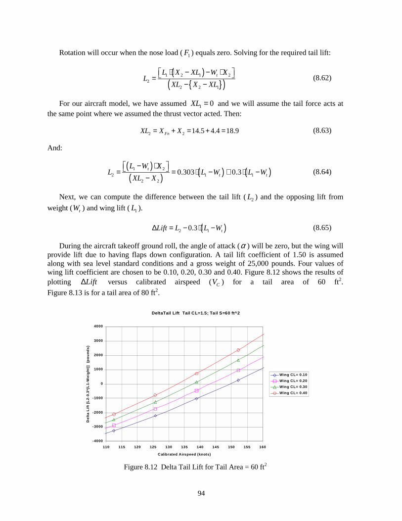
94

Rotation will occur when the nose load ( 1F ) equals zero. Solving for the required tail lift:

( )

{ }( )1 2 1 2

22 2 1

tL X XL W XL

XL X XL ⋅ − − ⋅ =

− − (8.62)

For our aircraft model, we have assumed 1 0XL = and we will assume the tail force acts at the same point where we assumed the thrust vector acted. Then:

2 2 14.5 4.4 18.9FnXL X X= + = + = (8.63)

And:

( )( ) ( ) ( )1 2

2 1 12 2

0.303 0.3tt t

L W XL L W L W

XL X − ⋅ = = ⋅ − ≅ ⋅ −

− (8.64)

Next, we can compute the difference between the tail lift ( 2L ) and the opposing lift from weight ( tW ) and wing lift ( 1L ).

( )2 10.3 tLift L L W∆ = − ⋅ − (8.65)

During the aircraft takeoff ground roll, the angle of attack (α ) will be zero, but the wing will provide lift due to having flaps down configuration. A tail lift coefficient of 1.50 is assumed along with sea level standard conditions and a gross weight of 25,000 pounds. Four values of wing lift coefficient are chosen to be 0.10, 0.20, 0.30 and 0.40. Figure 8.12 shows the results of plotting Lift∆ versus calibrated airspeed ( CV ) for a tail area of 60 ft2. Figure 8.13 is for a tail area of 80 ft2.

DeltaTail Lift Tail CL=1.5; Tail S=60 ft^2

-4000

-3000

-2000

-1000

0

1000

2000

3000

4000

110 115 120 125 130 135 140 145 150 155 160

Calibrated Airspeed (knots)

Del

ta L

ift

[L2-

0.3*

(L1-

Wei

ght

)] (

po

und

s)

Wing CL= 0.10Wing CL= 0.20Wing CL= 0.30Wing CL= 0.40

Figure 8.12 Delta Tail Lift for Tail Area = 60 ft2

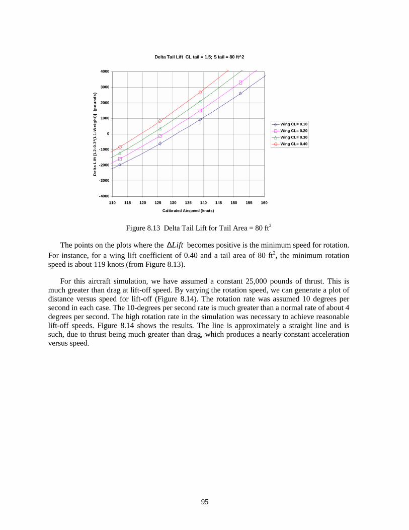
95

Delta Tail Lift CL tail = 1.5; S tail = 80 ft^2

-4000

-3000

-2000

-1000

0

1000

2000

3000

4000

110 115 120 125 130 135 140 145 150 155 160

Calibrated Airspeed (knots)

Del

ta L

ift

[L2-

0.3*

(L1-

Wei

ght

)] (

po

und

s)

Wing CL= 0.10Wing CL= 0.20Wing CL= 0.30Wing CL= 0.40

Figure 8.13 Delta Tail Lift for Tail Area = 80 ft2

The points on the plots where the Lift∆ becomes positive is the minimum speed for rotation. For instance, for a wing lift coefficient of 0.40 and a tail area of 80 ft2, the minimum rotation speed is about 119 knots (from Figure 8.13).

For this aircraft simulation, we have assumed a constant 25,000 pounds of thrust. This is much greater than drag at lift-off speed. By varying the rotation speed, we can generate a plot of distance versus speed for lift-off (Figure 8.14). The rotation rate was assumed 10 degrees per second in each case. The 10-degrees per second rate is much greater than a normal rate of about 4 degrees per second. The high rotation rate in the simulation was necessary to achieve reasonable lift-off speeds. Figure 8.14 shows the results. The line is approximately a straight line and is such, due to thrust being much greater than drag, which produces a nearly constant acceleration versus speed.

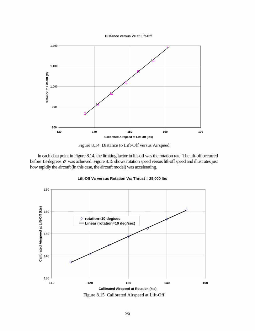
96

Distance versus Vc at Lift-Off

800

900

1,000

1,100

1,200

130 140 150 160 170


Dis

tanc

e to

Lift

-Off

(ft)

Figure 8.14 Distance to Lift-Off versus Airspeed

In each data point in Figure 8.14, the limiting factor in lift-off was the rotation rate. The lift-off occurred before 13-degrees α was achieved. Figure 8.15 shows rotation speed versus lift-off speed and illustrates just how rapidly the aircraft (in this case, the aircraft model) was accelerating.

Lift-Off Vc versus Rotation Vc: Thrust = 25,000 lbs

130

140

150

160

170

110 120 130 140 150Calibrated Airspeed at Rotation (kts)

Cal

ibra

ted

Airs

peed

at L

ift-O

ff (k

ts)

rotation=10 deg/secLinear (rotation=10 deg/sec)

Figure 8.15 Calibrated Airspeed at Lift-Off

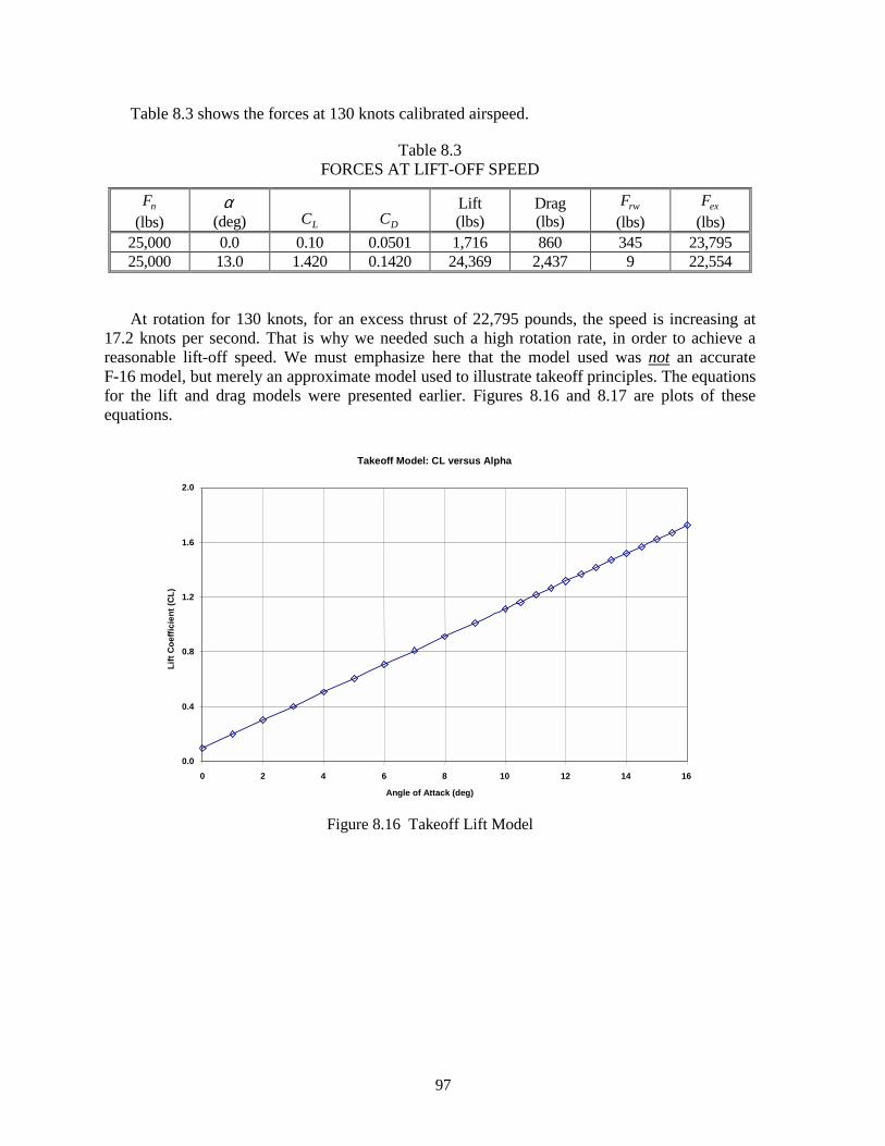
97

Table 8.3 shows the forces at 130 knots calibrated airspeed.

Table 8.3 FORCES AT LIFT-OFF SPEED

nF (lbs)

α (deg)

LC

DC

Lift (lbs)

Drag (lbs)

rwF (lbs)

exF (lbs)

25,000 0.0 0.10 0.0501 1,716 860 345 23,795 25,000 13.0 1.420 0.1420 24,369 2,437 9 22,554

At rotation for 130 knots, for an excess thrust of 22,795 pounds, the speed is increasing at 17.2 knots per second. That is why we needed such a high rotation rate, in order to achieve a reasonable lift-off speed. We must emphasize here that the model used was not an accurate F-16 model, but merely an approximate model used to illustrate takeoff principles. The equations for the lift and drag models were presented earlier. Figures 8.16 and 8.17 are plots of these equations.

Takeoff Model: CL versus Alpha

0.0

0.4

0.8

1.2

1.6

2.0

0 2 4 6 8 10 12 14 16

Angle of Attack (deg)

Lift

Coe

ffici

ent (

CL)

Figure 8.16 Takeoff Lift Model

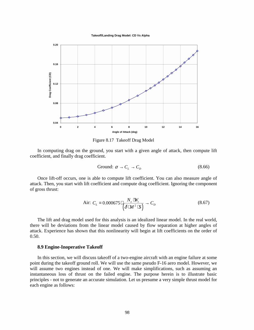
98

Takeoff/Landing Drag Model: CD Vs Alpha

0.04

0.08

0.12

0.16

0.20

0 2 4 6 8 10 12 14 16

Angle of Attack (deg)

Dra

g C

oeffi

cien

t (C

D)

Figure 8.17 Takeoff Drag Model

In computing drag on the ground, you start with a given angle of attack, then compute lift coefficient, and finally drag coefficient.

Ground: L DC Cα → → (8.66)

Once lift-off occurs, one is able to compute lift coefficient. You can also measure angle of attack. Then, you start with lift coefficient and compute drag coefficient. Ignoring the component of gross thrust:

Air: ( )2

0.000675 z tL D

N WC CM Sδ⋅= ⋅ →

⋅ ⋅ (8.67)

The lift and drag model used for this analysis is an idealized linear model. In the real world, there will be deviations from the linear model caused by flow separation at higher angles of attack. Experience has shown that this nonlinearity will begin at lift coefficients on the order of 0.50.

8.9 Engine-Inoperative Takeoff

In this section, we will discuss takeoff of a two-engine aircraft with an engine failure at some point during the takeoff ground roll. We will use the same pseudo F-16 aero model. However, we will assume two engines instead of one. We will make simplifications, such as assuming an instantaneous loss of thrust on the failed engine. The purpose herein is to illustrate basic principles - not to generate an accurate simulation. Let us presume a very simple thrust model for each engine as follows:

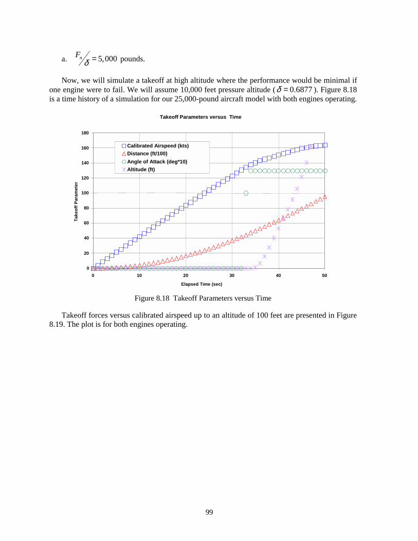
99

a. 5,000nFδ = pounds.

Now, we will simulate a takeoff at high altitude where the performance would be minimal if one engine were to fail. We will assume 10,000 feet pressure altitude ( 0.6877δ = ). Figure 8.18 is a time history of a simulation for our 25,000-pound aircraft model with both engines operating.

Takeoff Parameters versus Time

0

20

40

60

80

100

120

140

160

180

0 10 20 30 40 50

Elapsed Time (sec)

Take

off P

aram

eter

Calibrated Airspeed (kts)Distance (ft/100)Angle of Attack (deg*10)Altitude (ft)

Figure 8.18 Takeoff Parameters versus Time

Takeoff forces versus calibrated airspeed up to an altitude of 100 feet are presented in Figure 8.19. The plot is for both engines operating.

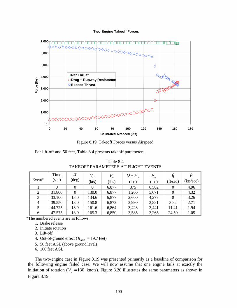
100

Two-Engine Takeoff Forces

0

1,000

2,000

3,000

4,000

5,000

6,000

7,000

0 20 40 60 80 100 120 140 160 180Calibrated Airspeed (kts)

Forc

e (lb

s)

Net ThrustDrag + Runway ResistanceExcess Thrust

Figure 8.19 Takeoff Forces versus Airspeed

For lift-off and 50 feet, Table 8.4 presents takeoff parameters.

Table 8.4 TAKEOFF PARAMETERS AT FLIGHT EVENTS

Event*

Time (sec)

α (deg)

CV (kts)

nF (lbs)

rwD F+ (lbs)

exF (lbs)

h! (ft/sec)

V! (kts/sec)

1 0 0 0 6,877 375 6,502 0 4.96 2 31.800 0 130.0 6,877 1,206 5,671 0 4.32 3 33.100 13.0 134.6 6,877 2,600 4,277 0 3.26 4 39.550 13.0 150.8 6,872 2,990 3,881 3.82 2.71 5 44.725 13.0 161.6 6,864 3,423 3,441 11.41 1.94 6 47.575 13.0 165.3 6,850 3,585 3,265 24.50 1.05

*The numbered events are as follows: 1. Brake release 2. Initiate rotation 3. Lift-off 4. Out-of-ground effect ( AGLh = 19.7 feet) 5. 50 feet AGL (above ground level) 6. 100 feet AGL

The two-engine case in Figure 8.19 was presented primarily as a baseline of comparison for

the following engine failed case. We will now assume that one engine fails at exactly the initiation of rotation ( 130CV = knots). Figure 8.20 illustrates the same parameters as shown in Figure 8.19.

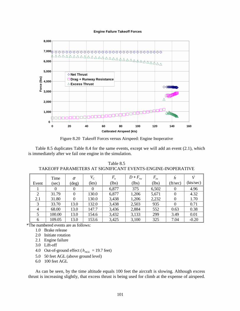
101

Engine Failure Takeoff Forces

0

1,000

2,000

3,000

4,000

5,000

6,000

7,000

8,000


Forc

e (lb

s)


Figure 8.20 Takeoff Forces versus Airspeed: Engine Inoperative

Table 8.5 duplicates Table 8.4 for the same events, except we will add an event (2.1), which is immediately after we fail one engine in the simulation.

Table 8.5 TAKEOFF PARAMETERS AT SIGNIFICANT EVENTS-ENGINE-INOPERATIVE

Event

Time (sec)

α (deg)

CV (kts)

nF (lbs)

rwD F+ (lbs)

exF (lbs)

h! (ft/sec)

V! (kts/sec)

1 0 0 0 6,877 375 6,502 0 4.96 2

2.1 31.79 31.80

0 0

130.0 130.0

6,877 3,438

1,206 1,206

5,671 2,232

0 0

4.32 1.70

3 33.70 13.0 132.0 3,438 2,503 935 0 0.71 4 68.00 13.0 147.7 3,436 2,884 552 0.63 0.38 5 100.00 13.0 154.6 3,432 3,133 299 3.49 0.01 6 109.05 13.0 153.6 3,425 3,100 325 7.04 -0.20

*The numbered events are as follows: 1.0 Brake release 2.0 Initiate rotation 2.1 Engine failure 3.0 Lift-off 4.0 Out-of-ground effect ( AGLh = 19.7 feet) 5.0 50 feet AGL (above ground level) 6.0 100 feet AGL

As can be seen, by the time altitude equals 100 feet the aircraft is slowing. Although excess

thrust is increasing slightly, that excess thrust is being used for climb at the expense of airspeed.

102

In case of an engine failure in such a scenario, one would need to reduce the drag and pitch over to reduce rate of climb. The drag reduction would be accomplished by raising the gear. Then, conduct a low-g turn (to minimize drag) and return to base for landing. This is just one possible option. The aircraft flight manual would contain the recommended emergency procedure.

8.10 Idle Thrust Decelerations

To assist in the development (or verification) of a takeoff and landing simulation, idle thrust decelerations may be performed. One would accelerate the aircraft on the runway to some high airspeed. Then, cut the throttle to idle and allow the aircraft to freely decelerate. We can solve for drag ( D ) in the equation found in the Developing a Takeoff Simulation subsection and then put D into coefficient form. Lift and drag coefficients are discussed in the lift and drag section of this handbook.

[ ]sin( ) cos( )n ex t rw t rwD F F W W Lθ µ θ µ= − − ⋅ − ⋅ ⋅ + ⋅ (8.69)

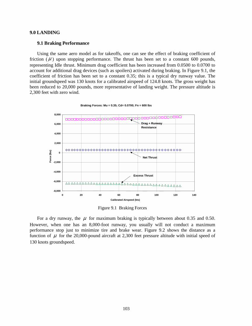
103

9.0 LANDING

9.1 Braking Performance

Using the same aero model as for takeoffs, one can see the effect of braking coefficient of friction (µ ) upon stopping performance. The thrust has been set to a constant 600 pounds, representing Idle thrust. Minimum drag coefficient has been increased from 0.0500 to 0.0700 to account for additional drag devices (such as spoilers) activated during braking. In Figure 9.1, the coefficient of friction has been set to a constant 0.35; this is a typical dry runway value. The initial groundspeed was 130 knots for a calibrated airspeed of 124.8 knots. The gross weight has been reduced to 20,000 pounds, more representative of landing weight. The pressure altitude is 2,300 feet with zero wind.

Braking Forces: Mu = 0.35; Cd= 0.0700; Fn = 600 lbs

-8,000

-6,000

-4,000

-2,000

0

2,000

4,000

6,000

8,000

0 20 40 60 80 100 120 140


Forc

e (lb

s)

Drag + RunwayResistance

Net Thrust

Excess Thrust

Figure 9.1 Braking Forces

For a dry runway, the µ for maximum braking is typically between about 0.35 and 0.50. However, when one has an 8,000-foot runway, you usually will not conduct a maximum performance stop just to minimize tire and brake wear. Figure 9.2 shows the distance as a function of µ for the 20,000-pound aircraft at 2,300 feet pressure altitude with initial speed of 130 knots groundspeed.

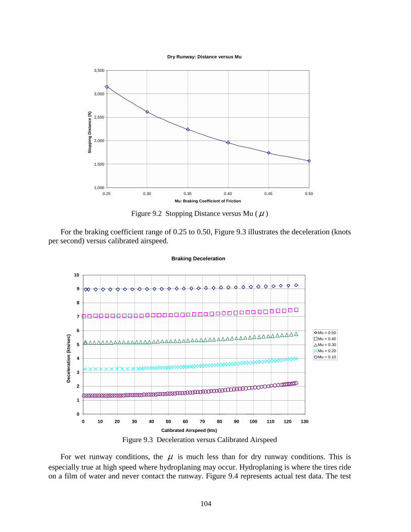
104

Dry Runway: Distance versus Mu

1,000

1,500

2,000

2,500

3,000

3,500

0.25 0.30 0.35 0.40 0.45 0.50

Mu: Braking Coefficient of Friction

Stop

ping

Dis

tanc

e (ft

)

Figure 9.2 Stopping Distance versus Mu (µ )

For the braking coefficient range of 0.25 to 0.50, Figure 9.3 illustrates the deceleration (knots per second) versus calibrated airspeed.

Braking Deceleration

0

1

2

3

4

5

6

7

8

9

10

0 10 20 30 40 50 60 70 80 90 100 110 120 130


Dec

eler

atio

n (k

ts/s

ec) Mu = 0.50

Mu = 0.40Mu = 0.30Mu = 0.20Mu = 0.10

Figure 9.3 Deceleration versus Calibrated Airspeed

For wet runway conditions, the µ is much less than for dry runway conditions. This is especially true at high speed where hydroplaning may occur. Hydroplaning is where the tires ride on a film of water and never contact the runway. Figure 9.4 represents actual test data. The test

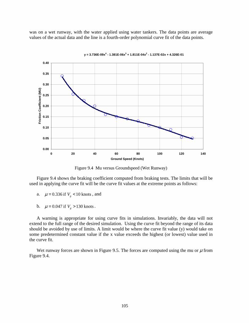
105

was on a wet runway, with the water applied using water tankers. The data points are average values of the actual data and the line is a fourth-order polynomial curve fit of the data points.

y = 3.736E-09x4 - 1.381E-06x3 + 1.811E-04x2 - 1.137E-02x + 4.326E-01

0.00

0.05

0.10

0.15

0.20

0.25

0.30

0.35

0.40

0 20 40 60 80 100 120 140Ground Speed (Knots)

Fric

tion

Coe

ffici

ent (

MU

)

Figure 9.4 Mu versus Groundspeed (Wet Runway)

Figure 9.4 shows the braking coefficient computed from braking tests. The limits that will be used in applying the curve fit will be the curve fit values at the extreme points as follows:

a. 0.336 if 10 knotsgVµ = < , and

b. 0.047 if 130 knotsgVµ = > .

A warning is appropriate for using curve fits in simulations. Invariably, the data will not extend to the full range of the desired simulation. Using the curve fit beyond the range of its data should be avoided by use of limits. A limit would be where the curve fit value (y) would take on some predetermined constant value if the x value exceeds the highest (or lowest) value used in the curve fit.

Wet runway forces are shown in Figure 9.5. The forces are computed using the mu or µ from Figure 9.4.

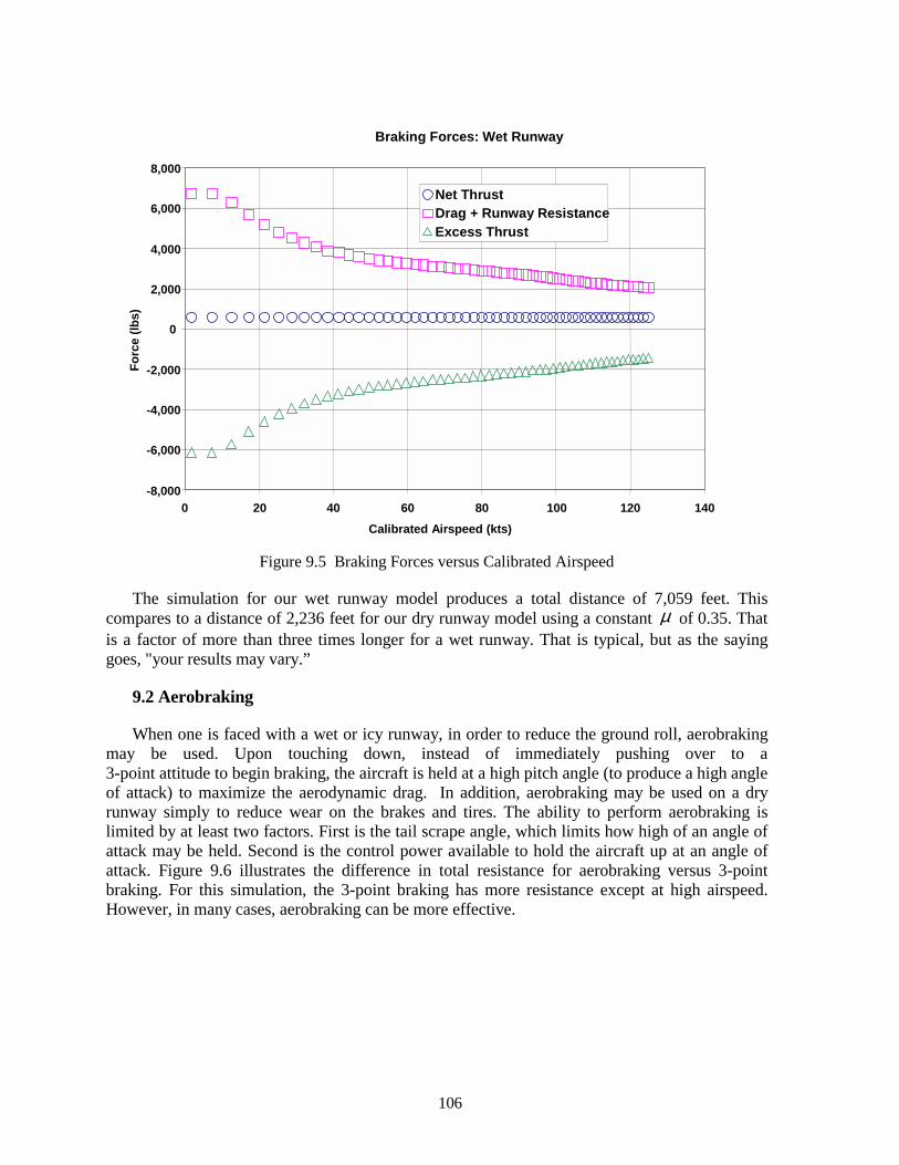
106

Braking Forces: Wet Runway

-8,000

-6,000

-4,000

-2,000

0

2,000

4,000

6,000

8,000

0 20 40 60 80 100 120 140Calibrated Airspeed (kts)

Forc

e (lb

s)


Figure 9.5 Braking Forces versus Calibrated Airspeed

The simulation for our wet runway model produces a total distance of 7,059 feet. This compares to a distance of 2,236 feet for our dry runway model using a constant µ of 0.35. That is a factor of more than three times longer for a wet runway. That is typical, but as the saying goes, "your results may vary.”

9.2 Aerobraking

When one is faced with a wet or icy runway, in order to reduce the ground roll, aerobraking may be used. Upon touching down, instead of immediately pushing over to a 3-point attitude to begin braking, the aircraft is held at a high pitch angle (to produce a high angle of attack) to maximize the aerodynamic drag. In addition, aerobraking may be used on a dry runway simply to reduce wear on the brakes and tires. The ability to perform aerobraking is limited by at least two factors. First is the tail scrape angle, which limits how high of an angle of attack may be held. Second is the control power available to hold the aircraft up at an angle of attack. Figure 9.6 illustrates the difference in total resistance for aerobraking versus 3-point braking. For this simulation, the 3-point braking has more resistance except at high airspeed. However, in many cases, aerobraking can be more effective.

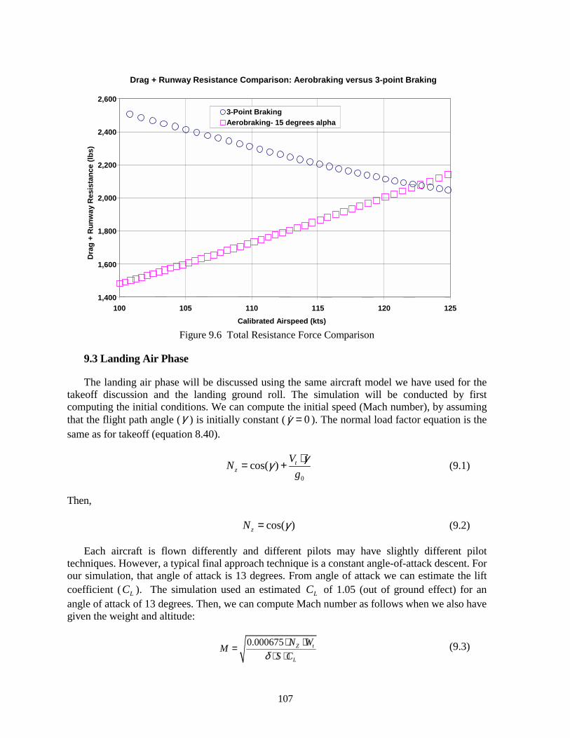
107

Drag + Runway Resistance Comparison: Aerobraking versus 3-point Braking

1,400

1,600

1,800

2,000

2,200

2,400

2,600

100 105 110 115 120 125Calibrated Airspeed (kts)

Dra

g +

Run

way

Res

ista

nce

(lbs)

3-Point BrakingAerobraking- 15 degrees alpha

Figure 9.6 Total Resistance Force Comparison

9.3 Landing Air Phase

The landing air phase will be discussed using the same aircraft model we have used for the takeoff discussion and the landing ground roll. The simulation will be conducted by first computing the initial conditions. We can compute the initial speed (Mach number), by assuming that the flight path angle (γ ) is initially constant ( 0γ =! ). The normal load factor equation is the same as for takeoff (equation 8.40).

0

cos( ) tz

VNgγγ ⋅= +!

(9.1)

Then,

cos( )zN γ= (9.2)

Each aircraft is flown differently and different pilots may have slightly different pilot techniques. However, a typical final approach technique is a constant angle-of-attack descent. For our simulation, that angle of attack is 13 degrees. From angle of attack we can estimate the lift coefficient ( LC ). The simulation used an estimated LC of 1.05 (out of ground effect) for an angle of attack of 13 degrees. Then, we can compute Mach number as follows when we also have given the weight and altitude:

0.000675 Z t

L

N WMS Cδ⋅ ⋅=

⋅ ⋅ (9.3)

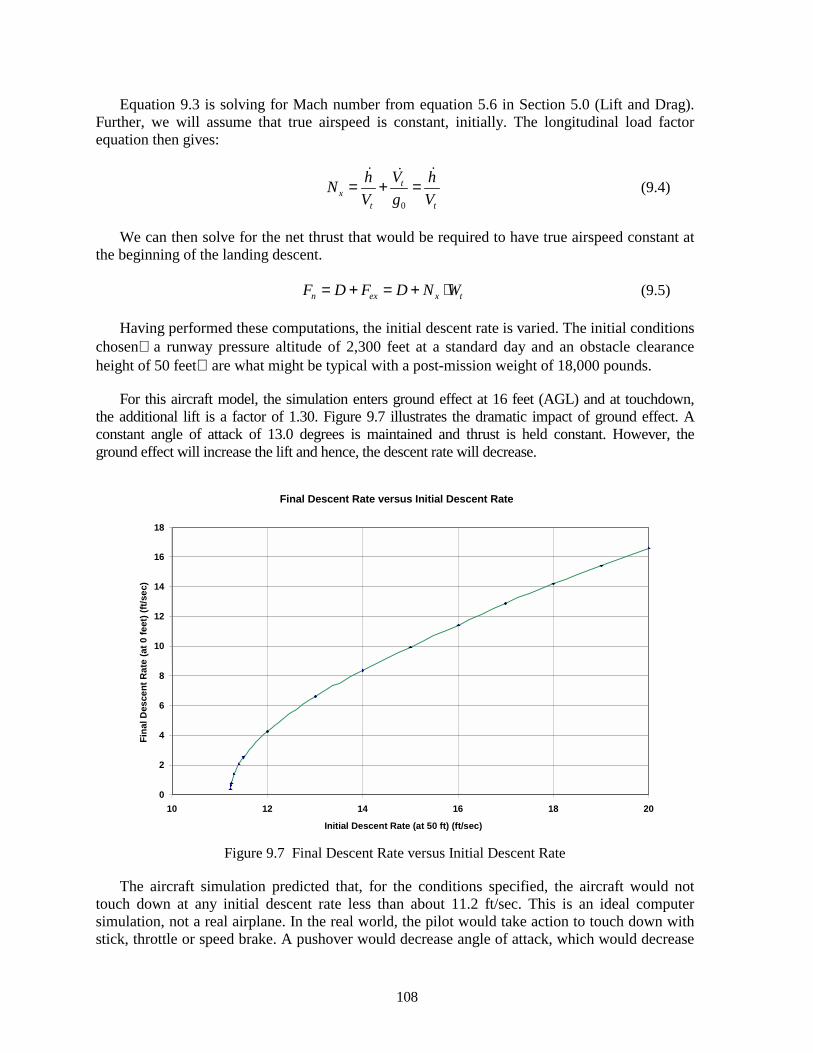
108

Equation 9.3 is solving for Mach number from equation 5.6 in Section 5.0 (Lift and Drag). Further, we will assume that true airspeed is constant, initially. The longitudinal load factor equation then gives:

0

tx

t t

Vh hNV g V

= + =! !!

(9.4)

We can then solve for the net thrust that would be required to have true airspeed constant at the beginning of the landing descent.

n ex x tF D F D N W= + = + ⋅ (9.5)

Having performed these computations, the initial descent rate is varied. The initial conditions chosen a runway pressure altitude of 2,300 feet at a standard day and an obstacle clearance height of 50 feet are what might be typical with a post-mission weight of 18,000 pounds.

For this aircraft model, the simulation enters ground effect at 16 feet (AGL) and at touchdown, the additional lift is a factor of 1.30. Figure 9.7 illustrates the dramatic impact of ground effect. A constant angle of attack of 13.0 degrees is maintained and thrust is held constant. However, the ground effect will increase the lift and hence, the descent rate will decrease.

Final Descent Rate versus Initial Descent Rate

0

2

4

6

8

10

12

14

16

18

10 12 14 16 18 20

Initial Descent Rate (at 50 ft) (ft/sec)

Fina

l Des

cent

Rat

e (a

t 0 fe

et) (

ft/se

c)

Figure 9.7 Final Descent Rate versus Initial Descent Rate

The aircraft simulation predicted that, for the conditions specified, the aircraft would not touch down at any initial descent rate less than about 11.2 ft/sec. This is an ideal computer simulation, not a real airplane. In the real world, the pilot would take action to touch down with stick, throttle or speed brake. A pushover would decrease angle of attack, which would decrease

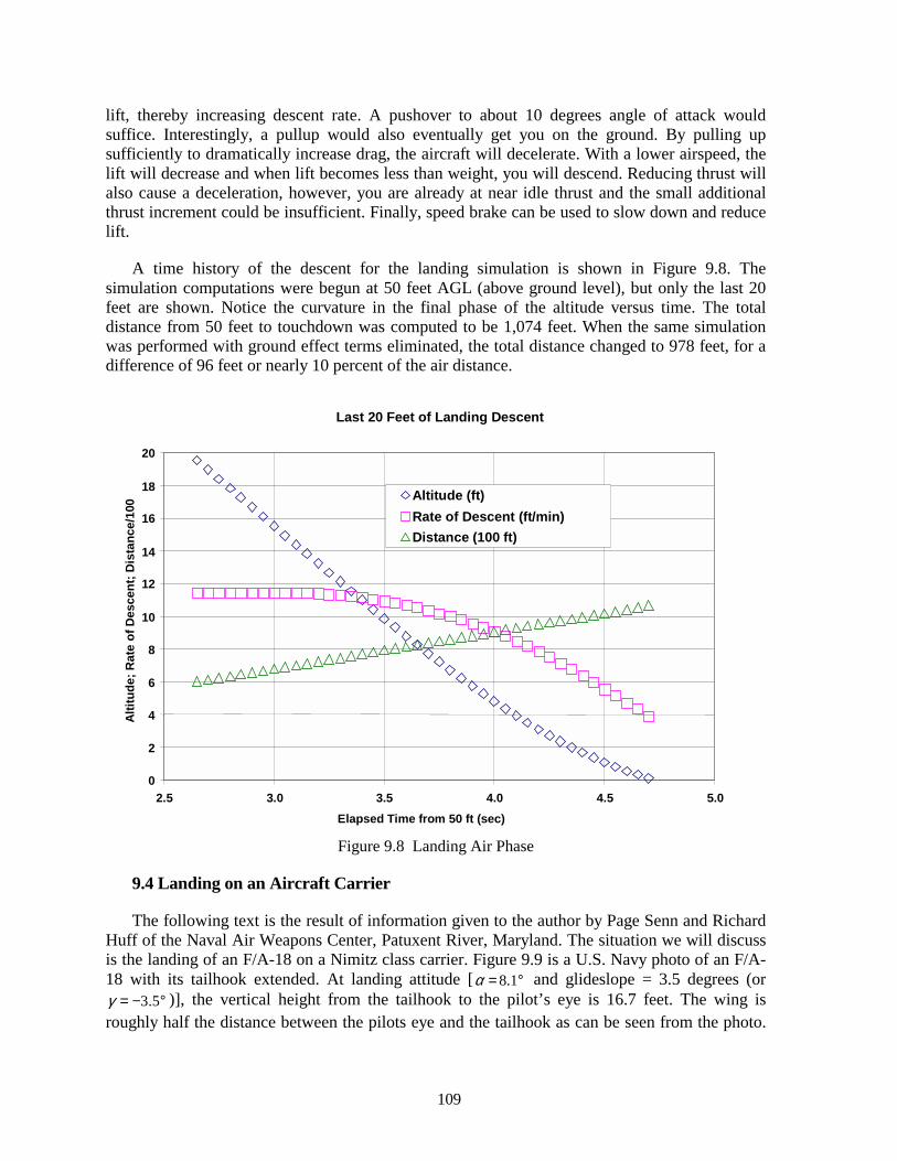
109

lift, thereby increasing descent rate. A pushover to about 10 degrees angle of attack would suffice. Interestingly, a pullup would also eventually get you on the ground. By pulling up sufficiently to dramatically increase drag, the aircraft will decelerate. With a lower airspeed, the lift will decrease and when lift becomes less than weight, you will descend. Reducing thrust will also cause a deceleration, however, you are already at near idle thrust and the small additional thrust increment could be insufficient. Finally, speed brake can be used to slow down and reduce lift.

A time history of the descent for the landing simulation is shown in Figure 9.8. The simulation computations were begun at 50 feet AGL (above ground level), but only the last 20 feet are shown. Notice the curvature in the final phase of the altitude versus time. The total distance from 50 feet to touchdown was computed to be 1,074 feet. When the same simulation was performed with ground effect terms eliminated, the total distance changed to 978 feet, for a difference of 96 feet or nearly 10 percent of the air distance.

Last 20 Feet of Landing Descent

0

2

4

6

8

10

12

14

16

18

20

2.5 3.0 3.5 4.0 4.5 5.0Elapsed Time from 50 ft (sec)

Altit

ude;

Rat

e of

Des

cent

; Dis

tanc

e/10

0 Altitude (ft)Rate of Descent (ft/min)Distance (100 ft)

Figure 9.8 Landing Air Phase

9.4 Landing on an Aircraft Carrier

The following text is the result of information given to the author by Page Senn and Richard Huff of the Naval Air Weapons Center, Patuxent River, Maryland. The situation we will discuss is the landing of an F/A-18 on a Nimitz class carrier. Figure 9.9 is a U.S. Navy photo of an F/A-18 with its tailhook extended. At landing attitude [ 8.1α = ° and glideslope = 3.5 degrees (or

3.5γ = − ° )], the vertical height from the tailhook to the pilot’s eye is 16.7 feet. The wing is roughly half the distance between the pilots eye and the tailhook as can be seen from the photo.

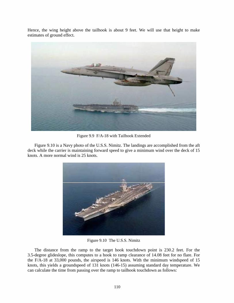
110

Hence, the wing height above the tailhook is about 9 feet. We will use that height to make estimates of ground effect.

Figure 9.9 F/A-18 with Tailhook Extended

Figure 9.10 is a Navy photo of the U.S.S. Nimitz. The landings are accomplished from the aft deck while the carrier is maintaining forward speed to give a minimum wind over the deck of 15 knots. A more normal wind is 25 knots.

Figure 9.10 The U.S.S. Nimitz

The distance from the ramp to the target hook touchdown point is 230.2 feet. For the 3.5-degree glideslope, this computes to a hook to ramp clearance of 14.08 feet for no flare. For the F/A-18 at 33,000 pounds, the airspeed is 146 knots. With the minimum windspeed of 15 knots, this yields a groundspeed of 131 knots (146-15) assuming standard day temperature. We can calculate the time from passing over the ramp to tailhook touchdown as follows:

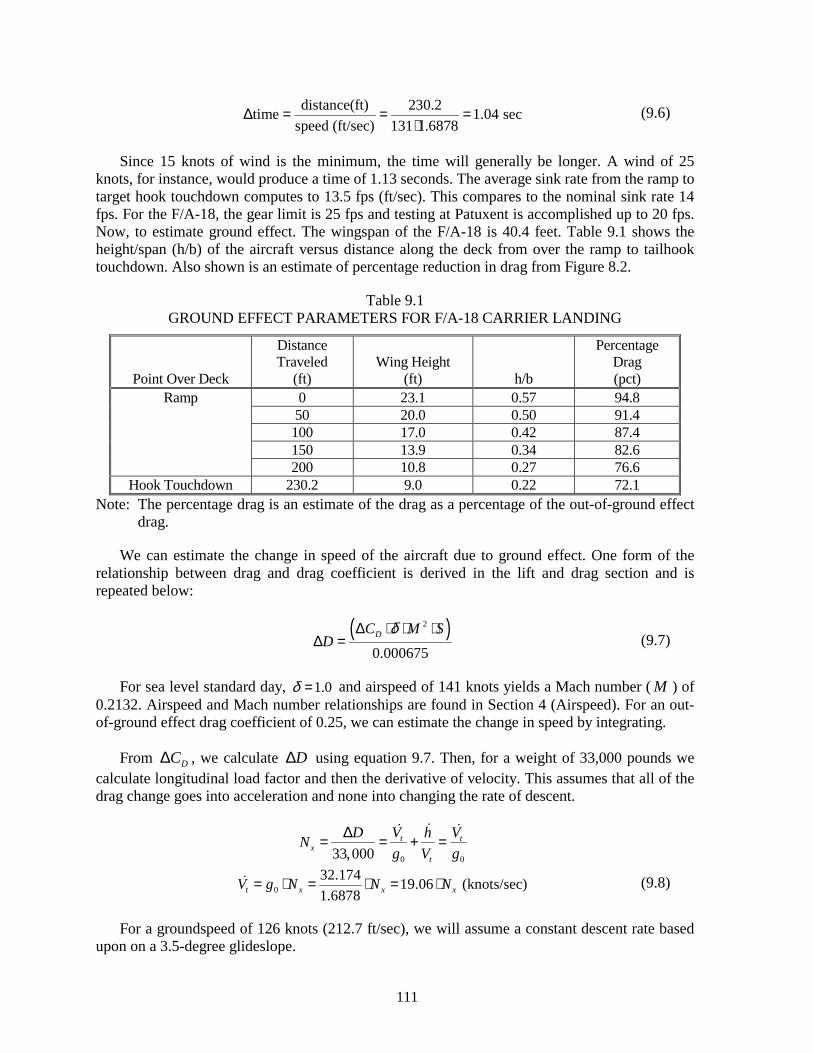
111

distance(ft) 230.2time 1.04 secspeed (ft/sec) 131 1.6878

∆ = = =⋅

(9.6)

Since 15 knots of wind is the minimum, the time will generally be longer. A wind of 25 knots, for instance, would produce a time of 1.13 seconds. The average sink rate from the ramp to target hook touchdown computes to 13.5 fps (ft/sec). This compares to the nominal sink rate 14 fps. For the F/A-18, the gear limit is 25 fps and testing at Patuxent is accomplished up to 20 fps. Now, to estimate ground effect. The wingspan of the F/A-18 is 40.4 feet. Table 9.1 shows the height/span (h/b) of the aircraft versus distance along the deck from over the ramp to tailhook touchdown. Also shown is an estimate of percentage reduction in drag from Figure 8.2.

Table 9.1 GROUND EFFECT PARAMETERS FOR F/A-18 CARRIER LANDING

Point Over Deck

Distance Traveled

(ft)

Wing Height

(ft)

h/b

Percentage Drag (pct)

0 23.1 0.57 94.8 50 20.0 0.50 91.4 100 17.0 0.42 87.4 150 13.9 0.34 82.6

Ramp

200 10.8 0.27 76.6 Hook Touchdown 230.2 9.0 0.22 72.1

Note: The percentage drag is an estimate of the drag as a percentage of the out-of-ground effect drag.

We can estimate the change in speed of the aircraft due to ground effect. One form of the relationship between drag and drag coefficient is derived in the lift and drag section and is repeated below:

( )2

0.000675DC M S

Dδ∆ ⋅ ⋅ ⋅

∆ = (9.7)

For sea level standard day, 1.0δ = and airspeed of 141 knots yields a Mach number ( M ) of 0.2132. Airspeed and Mach number relationships are found in Section 4 (Airspeed). For an out-of-ground effect drag coefficient of 0.25, we can estimate the change in speed by integrating.

From DC∆ , we calculate D∆ using equation 9.7. Then, for a weight of 33,000 pounds we calculate longitudinal load factor and then the derivative of velocity. This assumes that all of the drag change goes into acceleration and none into changing the rate of descent.

0 033,000t t

xt

V VD hNg V g

∆= = + =!! !

032.174 19.06 (knots/sec)1.6878t x x xV g N N N= ⋅ = ⋅ = ⋅! (9.8)

For a groundspeed of 126 knots (212.7 ft/sec), we will assume a constant descent rate based upon on a 3.5-degree glideslope.

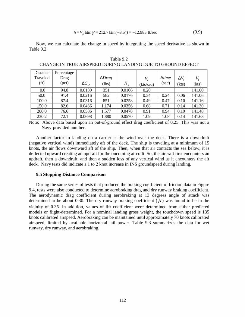
112

sin 212.7 sin( 3.5 ) 12.985 ft/secgh V γ= ⋅ = ⋅ − ° = −! (9.9)

Now, we can calculate the change in speed by integrating the speed derivative as shown in Table 9.2.

Table 9.2 CHANGE IN TRUE AIRSPEED DURING LANDING DUE TO GROUND EFFECT

Distance Traveled

(ft)

Percentage Drag (pct)

DC∆

Drag∆ (lbs)

xN

tV!

(kts/sec)

time∆

(sec)

tV∆

(kts)

tV

(kts) 0.0 94.8 0.0130 351 0.0106 0.20 141.00

50.0 91.4 0.0216 582 0.0176 0.34 0.24 0.06 141.06 100.0 87.4 0.0316 851 0.0258 0.49 0.47 0.10 141.16 150.0 82.6 0.0436 1,174 0.0356 0.68 0.71 0.14 141.30 200.0 76.6 0.0586 1,577 0.0478 0.91 0.94 0.19 141.48 230.2 72.1 0.0698 1,880 0.0570 1.09 1.08 0.14 141.63

Note: Above data based upon an out-of-ground effect drag coefficient of 0.25. This was not a Navy-provided number.

Another factor in landing on a carrier is the wind over the deck. There is a downdraft (negative vertical wind) immediately aft of the deck. The ship is traveling at a minimum of 15 knots, the air flows downward aft of the ship. Then, when that air contacts the sea below, it is deflected upward creating an updraft for the oncoming aircraft. So, the aircraft first encounters an updraft, then a downdraft, and then a sudden loss of any vertical wind as it encounters the aft deck. Navy tests did indicate a 1 to 2 knot increase in INS groundspeed during landing.

9.5 Stopping Distance Comparison

During the same series of tests that produced the braking coefficient of friction data in Figure 9.4, tests were also conducted to determine aerobraking drag and dry runway braking coefficient. The aerodynamic drag coefficient during aerobraking at 13 degrees angle of attack was determined to be about 0.30. The dry runway braking coefficient (µ ) was found to be in the vicinity of 0.35. In addition, values of lift coefficient were determined from either predicted models or flight-determined. For a nominal landing gross weight, the touchdown speed is 135 knots calibrated airspeed. Aerobraking can be maintained until approximately 70 knots calibrated airspeed, limited by available horizontal tail power. Table 9.3 summarizes the data for wet runway, dry runway, and aerobraking.

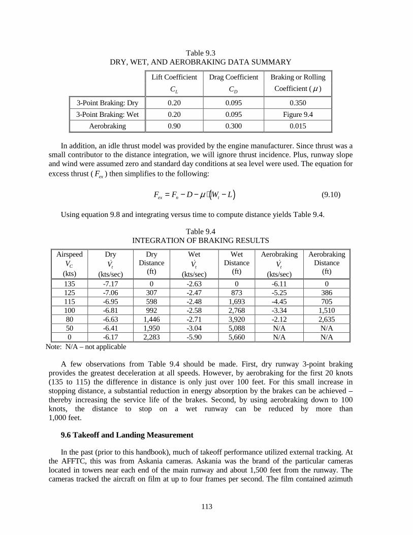
113

Table 9.3 DRY, WET, AND AEROBRAKING DATA SUMMARY

Lift Coefficient

LC Drag Coefficient

DC Braking or Rolling

Coefficient ( µ )

3-Point Braking: Dry 0.20 0.095 0.350 3-Point Braking: Wet 0.20 0.095 Figure 9.4

Aerobraking 0.90 0.300 0.015

In addition, an idle thrust model was provided by the engine manufacturer. Since thrust was a small contributor to the distance integration, we will ignore thrust incidence. Plus, runway slope and wind were assumed zero and standard day conditions at sea level were used. The equation for excess thrust ( exF ) then simplifies to the following:

( )ex n tF F D W Lµ= − − ⋅ − (9.10)

Using equation 9.8 and integrating versus time to compute distance yields Table 9.4.

Table 9.4 INTEGRATION OF BRAKING RESULTS

Airspeed CV

(kts)

Dry tV!

(kts/sec)

Dry Distance

(ft)

Wet tV!

(kts/sec)

Wet Distance

(ft)

Aerobraking tV!

(kts/sec)

Aerobraking Distance

(ft)

135 -7.17 0 -2.63 0 -6.11 0 125 -7.06 307 -2.47 873 -5.25 386 115 -6.95 598 -2.48 1,693 -4.45 705 100 -6.81 992 -2.58 2,768 -3.34 1,510 80 -6.63 1,446 -2.71 3,920 -2.12 2,635 50 -6.41 1,950 -3.04 5,088 N/A N/A 0 -6.17 2,283 -5.90 5,660 N/A N/A

Note: N/A – not applicable

A few observations from Table 9.4 should be made. First, dry runway 3-point braking provides the greatest deceleration at all speeds. However, by aerobraking for the first 20 knots (135 to 115) the difference in distance is only just over 100 feet. For this small increase in stopping distance, a substantial reduction in energy absorption by the brakes can be achieved – thereby increasing the service life of the brakes. Second, by using aerobraking down to 100 knots, the distance to stop on a wet runway can be reduced by more than 1,000 feet.

9.6 Takeoff and Landing Measurement

In the past (prior to this handbook), much of takeoff performance utilized external tracking. At the AFFTC, this was from Askania cameras. Askania was the brand of the particular cameras located in towers near each end of the main runway and about 1,500 feet from the runway. The cameras tracked the aircraft on film at up to four frames per second. The film contained azimuth

114

and elevation data. The film was developed, read, and computer-processed. The computer output included time, distance, velocity, acceleration, and altitude.

Now, with the advent of INS and GPS, the onboard inertial velocity data can be integrated to provide distance.

gd V dt= ⋅∫ (9.11)

where:

gV = horizontal component of groundspeed.

Altitude would be determined by integrating the vertical velocity, beginning at the point where lift-off occurred. The precise determination of the lift-off point would involve additional onboard instrumentation such main gear loads or wheel speed.

vh V dt∆ = ⋅∫ = altitude above the lift-off point (9.12)

where:

vV = vertical component of groundspeed.

Since the INS is subject to small drift errors, it is necessary to subtract out any null error. For the horizontal distance, this is obtained by simply collecting data when the aircraft was stopped. For the height integration, the vertical velocity at the lift-off point would be subtracted out. The GPS does not have a null error. A new device called an EGI (embedded GPS/INS) combines the outputs of both an INS and a GPS using a filter.

To compute acceleration, it is recommended to differentiate the velocities rather than use a direct output of the INS. That is because the INS is sensitive to body axis vibrations of the aircraft and the acceleration data will be very noisy due to this vibration. Typically, an INS will internally integrate the accelerations at a sample rate of at least 50 samples per second. By sampling the INS velocities at no more than 5 samples per second, you can essentially average out the noise in the data. The topic of noise in accelerometer data is discussed within the flight path acceleration heading of the excess thrust section. Then, the longitudinal acceleration can be determined with something as simple as a central difference derivative method.

( ) ( ) ( )( )( ) ( )( )

1 11 1

g gx

V i V iA i

t i t i+ − −

=+ − −

(9.13)

where:

i = the 'i th time sample.

Improved integration results would be produced using a moving second-order polynomial curve fit; a data process used by the AFFTC.

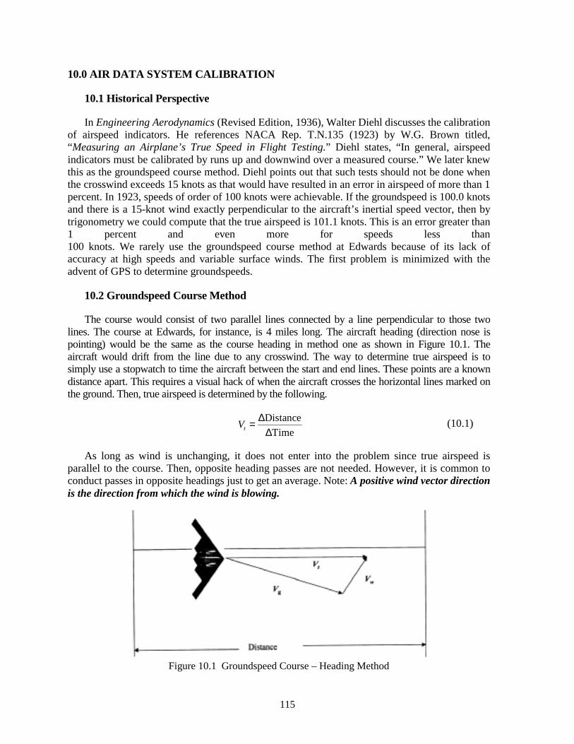
115

10.0 AIR DATA SYSTEM CALIBRATION

10.1 Historical Perspective

In Engineering Aerodynamics (Revised Edition, 1936), Walter Diehl discusses the calibration of airspeed indicators. He references NACA Rep. T.N.135 (1923) by W.G. Brown titled, “Measuring an Airplane’s True Speed in Flight Testing.” Diehl states, “In general, airspeed indicators must be calibrated by runs up and downwind over a measured course.” We later knew this as the groundspeed course method. Diehl points out that such tests should not be done when the crosswind exceeds 15 knots as that would have resulted in an error in airspeed of more than 1 percent. In 1923, speeds of order of 100 knots were achievable. If the groundspeed is 100.0 knots and there is a 15-knot wind exactly perpendicular to the aircraft’s inertial speed vector, then by trigonometry we could compute that the true airspeed is 101.1 knots. This is an error greater than 1 percent and even more for speeds less than 100 knots. We rarely use the groundspeed course method at Edwards because of its lack of accuracy at high speeds and variable surface winds. The first problem is minimized with the advent of GPS to determine groundspeeds.

10.2 Groundspeed Course Method

The course would consist of two parallel lines connected by a line perpendicular to those two lines. The course at Edwards, for instance, is 4 miles long. The aircraft heading (direction nose is pointing) would be the same as the course heading in method one as shown in Figure 10.1. The aircraft would drift from the line due to any crosswind. The way to determine true airspeed is to simply use a stopwatch to time the aircraft between the start and end lines. These points are a known distance apart. This requires a visual hack of when the aircraft crosses the horizontal lines marked on the ground. Then, true airspeed is determined by the following.

DistanceTimetV ∆=

∆ (10.1)

As long as wind is unchanging, it does not enter into the problem since true airspeed is parallel to the course. Then, opposite heading passes are not needed. However, it is common to conduct passes in opposite headings just to get an average. Note: A positive wind vector direction is the direction from which the wind is blowing.

Figure 10.1 Groundspeed Course – Heading Method

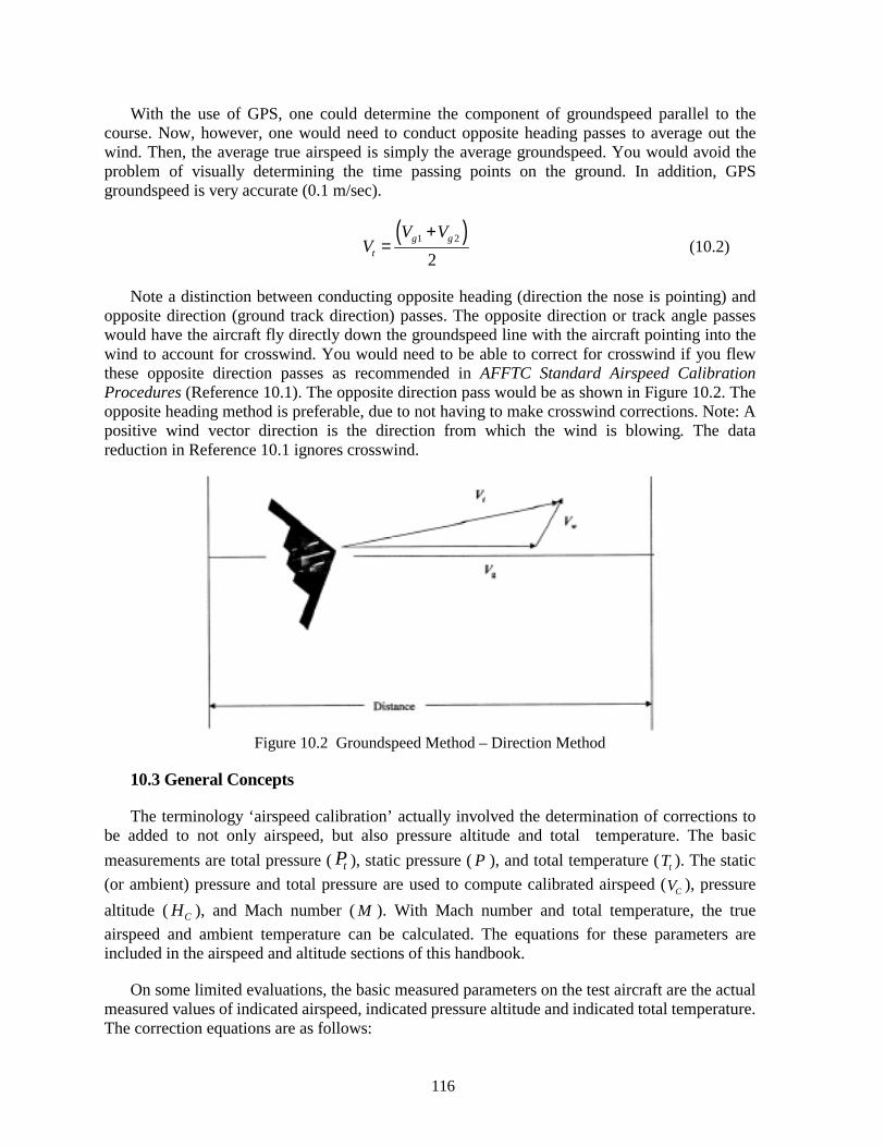
116

With the use of GPS, one could determine the component of groundspeed parallel to the course. Now, however, one would need to conduct opposite heading passes to average out the wind. Then, the average true airspeed is simply the average groundspeed. You would avoid the problem of visually determining the time passing points on the ground. In addition, GPS groundspeed is very accurate (0.1 m/sec).

( )1 2

2g g

t

V VV

+= (10.2)

Note a distinction between conducting opposite heading (direction the nose is pointing) and opposite direction (ground track direction) passes. The opposite direction or track angle passes would have the aircraft fly directly down the groundspeed line with the aircraft pointing into the wind to account for crosswind. You would need to be able to correct for crosswind if you flew these opposite direction passes as recommended in AFFTC Standard Airspeed Calibration Procedures (Reference 10.1). The opposite direction pass would be as shown in Figure 10.2. The opposite heading method is preferable, due to not having to make crosswind corrections. Note: A positive wind vector direction is the direction from which the wind is blowing. The data reduction in Reference 10.1 ignores crosswind.

Figure 10.2 Groundspeed Method – Direction Method

10.3 General Concepts

The terminology ‘airspeed calibration’ actually involved the determination of corrections to be added to not only airspeed, but also pressure altitude and total temperature. The basic measurements are total pressure ( tP ), static pressure ( P ), and total temperature ( tT ). The static (or ambient) pressure and total pressure are used to compute calibrated airspeed ( CV ), pressure altitude ( CH ), and Mach number ( M ). With Mach number and total temperature, the true airspeed and ambient temperature can be calculated. The equations for these parameters are included in the airspeed and altitude sections of this handbook.

On some limited evaluations, the basic measured parameters on the test aircraft are the actual measured values of indicated airspeed, indicated pressure altitude and indicated total temperature. The correction equations are as follows:

117

C i iC pCV V V V= + ∆ + ∆ calibrated airspeed (10.3)

C i iC pCH H H H= + ∆ + ∆ corrected pressure altitude (10.4)

t ti tiT T T= + ∆ total temperature (10.5)

where:

iCV∆ = instrument correction to indicated airspeed, pCV∆ = position error correction to instrument corrected airspeed,

iCH∆ = instrument correction to pressure altitude,

pCH∆ = position error correction to pressure altitude, and tiT∆ = instrument correction to total air temperature.

The modifier ‘corrected’ on pressure altitude is often dropped in practice. However, the modifier ‘calibrated’ on calibrated airspeed needs to be retained to distinguish it from true airspeed. When the parameters are instrument readings that not uncorrected for instrument and position errors then the modifier ‘indicated’ should be applied. The terminology ‘position error’ refers to the premise that there is some location on the aircraft to locate a sensor such that there would have been zero error in that measurement. However, there is no single position that would yield zero error at all Mach number and angle of attack.

When dealing with the three basic measurements ( , ,t tP P T ) on a test aircraft the i subscript referred to a measurement that had not been corrected for any instrumentation errors. The total temperature probe is also subject to an error called a probe recovery factor (η ). The relationship for total versus ambient temperature is as follows:

( )21 0.2tT T Mη= ⋅ + ⋅ ⋅ (10.6)

If, in flight test, one has an ambient temperature source (T ) and a total temperature measurement ( tT ) one could solve for η in the above equation and could calibrate the probe. The value for η is typically 0.98 to 1.00 for a well-designed system. However, in practical application with modern probes a value of 1.0 is frequently used.

The tT is the test aircraft’s measured total temperature. The ambient temperature (T ) would have been from another source. The other source could have been from another aircraft with a calibrated total temperature probe, from a weather balloon, or from a ground temperature measurement. The ground temperature measurement would be the source during tower flyby tests.

Weather balloon data would not be used as a primary calibration source. However, it makes an excellent check on your data system. Too many performance engineers ignore this valuable source of information. Appendix A contains weather balloon data from the Edwards AFB

118

weather squadron. The data illustrates average values of winds and temperatures versus month. There is also data from a sampling of 1 month of weather soundings.

A study conducted at Edwards AFB in the 1960s indicated that balloon temperature accuracies were on the order of ±2 degrees C.

The two pressure measurements could both have ‘position’ errors as follows:

t ti tiP P P= +∆ (10.7)

i sP P P= + ∆ (10.8)

Often, the symbology used here for ambient pressure ( P ) will be shown as ( sP ). The s would denote static. For purposes of this handbook static and ambient are considered the same thing.

In general, both of the pressure measurements are subject to errors. However, it is often assumed that there is zero total pressure error. In that case, all of the Pitot-static error is in the ambient pressure measurement. A position error parameter called delta p over q is defined as follows:

( )/ ip Cic

Cic

P PP q

q−

∆ = (10.9)

where:

Cicq = indicated compressible dynamic pressure, and

pP∆ = error in ambient pressure (position error).

With the assumption of zero total pressure error, the correction to be added to compressible dynamic pressure simplifies to the following:

C pq P∆ = −∆ (10.10)

At the AFFTC, a sign convention has been that a positive sign on pP∆ would produce a positive correction to be added to both calibrated airspeed ( CV∆ ) and pressure altitude ( CH∆ ). (One can avoid the confusion of a sign change by thinking of pP∆ as being a positive correction to be added to the compressible dynamic pressure ( Cq .) A positive correction to be added to ambient pressure would produce a negative correction to be added to both calibrated airspeed and to pressure altitude. So, one would need to change the sign on the ambient pressure correction as follows:

( ) ( )/ i i

p CicCic Cic

P P P PP q

q q− −

∆ = − = (10.11)

119

10.4 Pacer Aircraft

An aircraft that is utilized in the airspeed calibration of a test aircraft is called a pacer aircraft. The pacer will fly in formation with the test aircraft. The pacer’s computed values of calibrated airspeed ( CV ), pressure altitude ( CH ), and ambient temperature (T ) are compared to those three parameter values from the test aircraft. The test aircraft’s Pitot-static measurements are referred to as indicated values until a set of corrections can be determined by simply comparing to the pacers calibrated computed parameters. Just for simplicity, the computed ambient temperature is lumped with the pressure parameters and called Pitot-static parameters. The AFFTC pacer aircraft have onboard computers, which calculate instrumentation and position errors then add these corrections to the indicated values to present calibrated values. The position errors are the difference between the measured (or indicated) Pitot-static parameters and the true values.

Before pacer aircraft became the standard for Pitot-static measurement, it needed to be calibrated before it could be utilized in the airspeed calibration of test aircraft. One of the methods used in calibrating a pacer aircraft is to fly against another pacer aircraft. This has the potential of passing on errors from another pacer. To avoid that problem the new pacer is also tested using the tower flyby, accel-decel, and cloverleaf methods.

10.5 Tower Flyby

The tower flyby method of airspeed calibration consists of flying along a flyby line on the lakebed and passing by an observation tower perpendicular to the flyby line some 1,379 feet away (at Edwards AFB). An observer in the flyby tower watches the aircraft pass by the tower. With a grid on a window, the observer is able to compute the aircraft’s altitude above the tower zero grid line as the test aircraft passes in front of the grid on the window. Figure 10.3 shows an actual photo of an aircraft (F-18) passing by the Edwards AFB flyby tower.

A pressure altitude measurement in the tower is used to determine the zero grid line pressure altitude. Then, the pressure altitude of the aircraft is computed as follows:

/std

C a c p tower towerTH H hT

= + ∆ ⋅

pressure altitude for the aircraft (10.12)

where:

p towerH = pressure altitude measured at the zero grid line in the tower,

towerh∆ = geometric height of aircraft above the zero grid line measured by the tower,

stdT = standard day temperature (°K) at p towerH , and T = test day ambient temperature (°K).

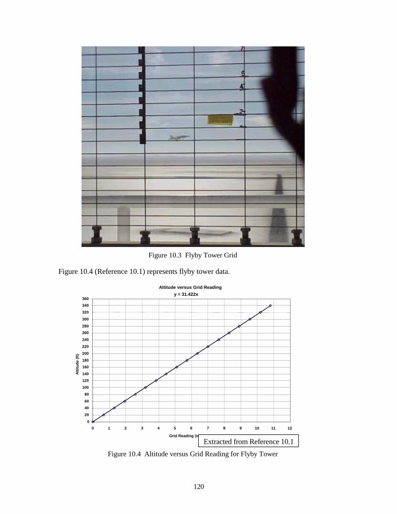
12

Figure 10.3 Flyby Tower Grid

Figure 10.4 (Reference 10.1) represents flyby tower data.

Altitude versus Grid Readingy = 31.422x

0

20

4060

80

100

120140

160180

200

220

240

260280

300

320

340360

0 1 2 3 4 5 6 7 8 9 10 11 12

Grid Reading (in

Alti

tude

(ft)

Figure 10.4 Altitude versus Gri

1
)
Extracted from Reference 10.

0

d Reading for Flyby Tower

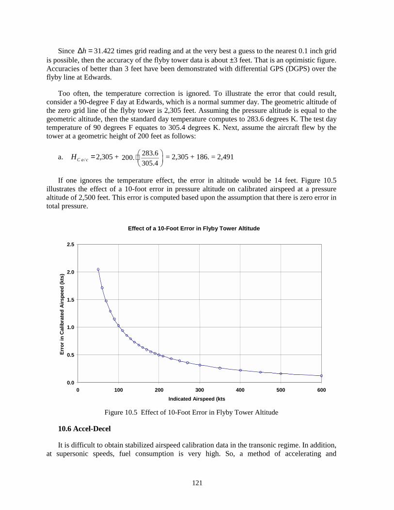
121

Since h∆ = 31.422 times grid reading and at the very best a guess to the nearest 0.1 inch grid is possible, then the accuracy of the flyby tower data is about ±3 feet. That is an optimistic figure. Accuracies of better than 3 feet have been demonstrated with differential GPS (DGPS) over the flyby line at Edwards.

Too often, the temperature correction is ignored. To illustrate the error that could result, consider a 90-degree F day at Edwards, which is a normal summer day. The geometric altitude of the zero grid line of the flyby tower is 2,305 feet. Assuming the pressure altitude is equal to the geometric altitude, then the standard day temperature computes to 283.6 degrees K. The test day temperature of 90 degrees F equates to 305.4 degrees K. Next, assume the aircraft flew by the tower at a geometric height of 200 feet as follows:

a. /C a cH =2,305 + 283.6200.305.4 ⋅

= 2,305 + 186. = 2,491

If one ignores the temperature effect, the error in altitude would be 14 feet. Figure 10.5 illustrates the effect of a 10-foot error in pressure altitude on calibrated airspeed at a pressure altitude of 2,500 feet. This error is computed based upon the assumption that there is zero error in total pressure.

Effect of a 10-Foot Error in Flyby Tower Altitude

0.0

0.5

1.0

1.5

2.0

2.5

0 100 200 300 400 500 600Indicated Airspeed (kts

Erro

r in

Cal

ibra

ted

Airs

peed

(kts

)

Figure 10.5 Effect of 10-Foot Error in Flyby Tower Altitude

10.6 Accel-Decel

It is difficult to obtain stabilized airspeed calibration data in the transonic regime. In addition, at supersonic speeds, fuel consumption is very high. So, a method of accelerating and

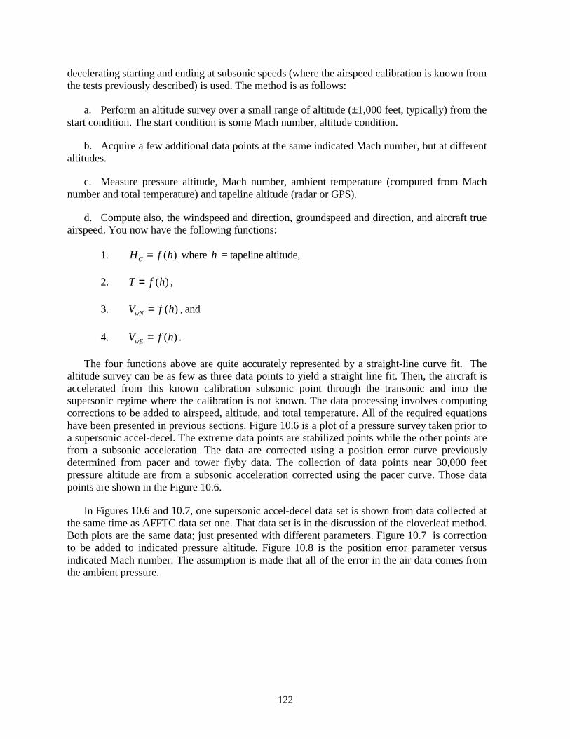
122

decelerating starting and ending at subsonic speeds (where the airspeed calibration is known from the tests previously described) is used. The method is as follows:

a. Perform an altitude survey over a small range of altitude (±1,000 feet, typically) from the start condition. The start condition is some Mach number, altitude condition.

b. Acquire a few additional data points at the same indicated Mach number, but at different altitudes.

c. Measure pressure altitude, Mach number, ambient temperature (computed from Mach number and total temperature) and tapeline altitude (radar or GPS).

d. Compute also, the windspeed and direction, groundspeed and direction, and aircraft true airspeed. You now have the following functions:

1. ( )CH f h= where h = tapeline altitude,

2. ( )T f h= ,

3. ( )wNV f h= , and

4. ( )wEV f h= .

The four functions above are quite accurately represented by a straight-line curve fit. The altitude survey can be as few as three data points to yield a straight line fit. Then, the aircraft is accelerated from this known calibration subsonic point through the transonic and into the supersonic regime where the calibration is not known. The data processing involves computing corrections to be added to airspeed, altitude, and total temperature. All of the required equations have been presented in previous sections. Figure 10.6 is a plot of a pressure survey taken prior to a supersonic accel-decel. The extreme data points are stabilized points while the other points are from a subsonic acceleration. The data are corrected using a position error curve previously determined from pacer and tower flyby data. The collection of data points near 30,000 feet pressure altitude are from a subsonic acceleration corrected using the pacer curve. Those data points are shown in the Figure 10.6.

In Figures 10.6 and 10.7, one supersonic accel-decel data set is shown from data collected at the same time as AFFTC data set one. That data set is in the discussion of the cloverleaf method. Both plots are the same data; just presented with different parameters. Figure 10.7 is correction to be added to indicated pressure altitude. Figure 10.8 is the position error parameter versus indicated Mach number. The assumption is made that all of the error in the air data comes from the ambient pressure.

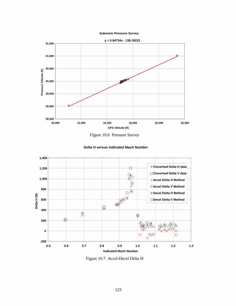
123

Subsonic Pressure Survey

y = 0.94734x - 138.18223

28,500

29,000

29,500

30,000

30,500

31,000

31,500

30,500 31,000 31,500 32,000 32,500 33,000

GPS Altitude (ft)

Pres

sure

Alti

tude

(ft)

Figure 10.6 Pressure Survey

Delta H versus Indicated Mach Number

-200

0

200

400

600

800

1,000

1,200

1,400

0.5 0.6 0.7 0.8 0.9 1.0 1.1 1.2 1.3Indicated Mach Number

Del

ta H

(ft)

Cloverleaf Delta H data

Cloverleaf Delta V data

Accel Delta H Method

Accel Delta V Method

Decel Delta H Method

Decel Delta V Method

Figure 10.7 Accel-Decel Delta H

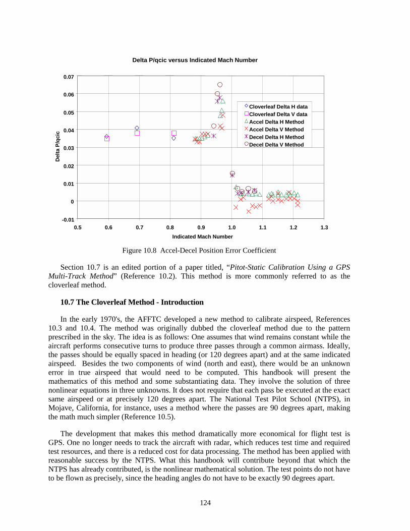
124

Delta P/qcic versus Indicated Mach Number

-0.01

0

0.01

0.02

0.03

0.04

0.05

0.06

0.07

0.5 0.6 0.7 0.8 0.9 1.0 1.1 1.2 1.3Indicated Mach Number

Del

ta P

/qci

c

Cloverleaf Delta H dataCloverleaf Delta V dataAccel Delta H MethodAccel Delta V MethodDecel Delta H MethodDecel Delta V Method

Figure 10.8 Accel-Decel Position Error Coefficient

Section 10.7 is an edited portion of a paper titled, “Pitot-Static Calibration Using a GPS Multi-Track Method” (Reference 10.2). This method is more commonly referred to as the cloverleaf method.

10.7 The Cloverleaf Method - Introduction

In the early 1970's, the AFFTC developed a new method to calibrate airspeed, References 10.3 and 10.4. The method was originally dubbed the cloverleaf method due to the pattern prescribed in the sky. The idea is as follows: One assumes that wind remains constant while the aircraft performs consecutive turns to produce three passes through a common airmass. Ideally, the passes should be equally spaced in heading (or 120 degrees apart) and at the same indicated airspeed. Besides the two components of wind (north and east), there would be an unknown error in true airspeed that would need to be computed. This handbook will present the mathematics of this method and some substantiating data. They involve the solution of three nonlinear equations in three unknowns. It does not require that each pass be executed at the exact same airspeed or at precisely 120 degrees apart. The National Test Pilot School (NTPS), in Mojave, California, for instance, uses a method where the passes are 90 degrees apart, making the math much simpler (Reference 10.5).

The development that makes this method dramatically more economical for flight test is GPS. One no longer needs to track the aircraft with radar, which reduces test time and required test resources, and there is a reduced cost for data processing. The method has been applied with reasonable success by the NTPS. What this handbook will contribute beyond that which the NTPS has already contributed, is the nonlinear mathematical solution. The test points do not have to be flown as precisely, since the heading angles do not have to be exactly 90 degrees apart.

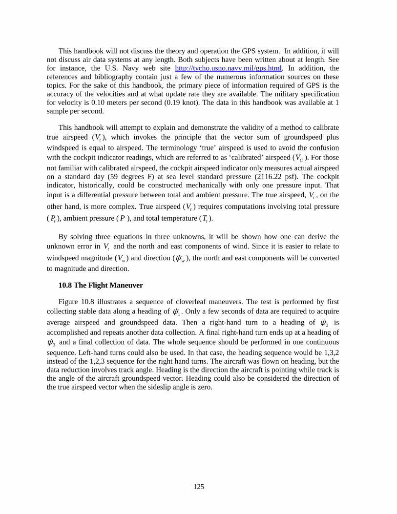
125

This handbook will not discuss the theory and operation the GPS system. In addition, it will not discuss air data systems at any length. Both subjects have been written about at length. See for instance, the U.S. Navy web site http://tycho.usno.navy.mil/gps.html. In addition, the references and bibliography contain just a few of the numerous information sources on these topics. For the sake of this handbook, the primary piece of information required of GPS is the accuracy of the velocities and at what update rate they are available. The military specification for velocity is 0.10 meters per second (0.19 knot). The data in this handbook was available at 1 sample per second.

This handbook will attempt to explain and demonstrate the validity of a method to calibrate true airspeed ( tV ), which invokes the principle that the vector sum of groundspeed plus windspeed is equal to airspeed. The terminology ‘true’ airspeed is used to avoid the confusion with the cockpit indicator readings, which are referred to as ‘calibrated’ airspeed ( CV ). For those not familiar with calibrated airspeed, the cockpit airspeed indicator only measures actual airspeed on a standard day (59 degrees F) at sea level standard pressure (2116.22 psf). The cockpit indicator, historically, could be constructed mechanically with only one pressure input. That input is a differential pressure between total and ambient pressure. The true airspeed, tV , on the other hand, is more complex. True airspeed ( tV ) requires computations involving total pressure ( tP ), ambient pressure ( P ), and total temperature ( tT ).

By solving three equations in three unknowns, it will be shown how one can derive the unknown error in tV and the north and east components of wind. Since it is easier to relate to windspeed magnitude ( wV ) and direction ( wψ ), the north and east components will be converted to magnitude and direction.

10.8 The Flight Maneuver

Figure 10.8 illustrates a sequence of cloverleaf maneuvers. The test is performed by first collecting stable data along a heading of 1ψ . Only a few seconds of data are required to acquire average airspeed and groundspeed data. Then a right-hand turn to a heading of 2ψ is accomplished and repeats another data collection. A final right-hand turn ends up at a heading of

3ψ and a final collection of data. The whole sequence should be performed in one continuous sequence. Left-hand turns could also be used. In that case, the heading sequence would be 1,3,2 instead of the 1,2,3 sequence for the right hand turns. The aircraft was flown on heading, but the data reduction involves track angle. Heading is the direction the aircraft is pointing while track is the angle of the aircraft groundspeed vector. Heading could also be considered the direction of the true airspeed vector when the sideslip angle is zero.

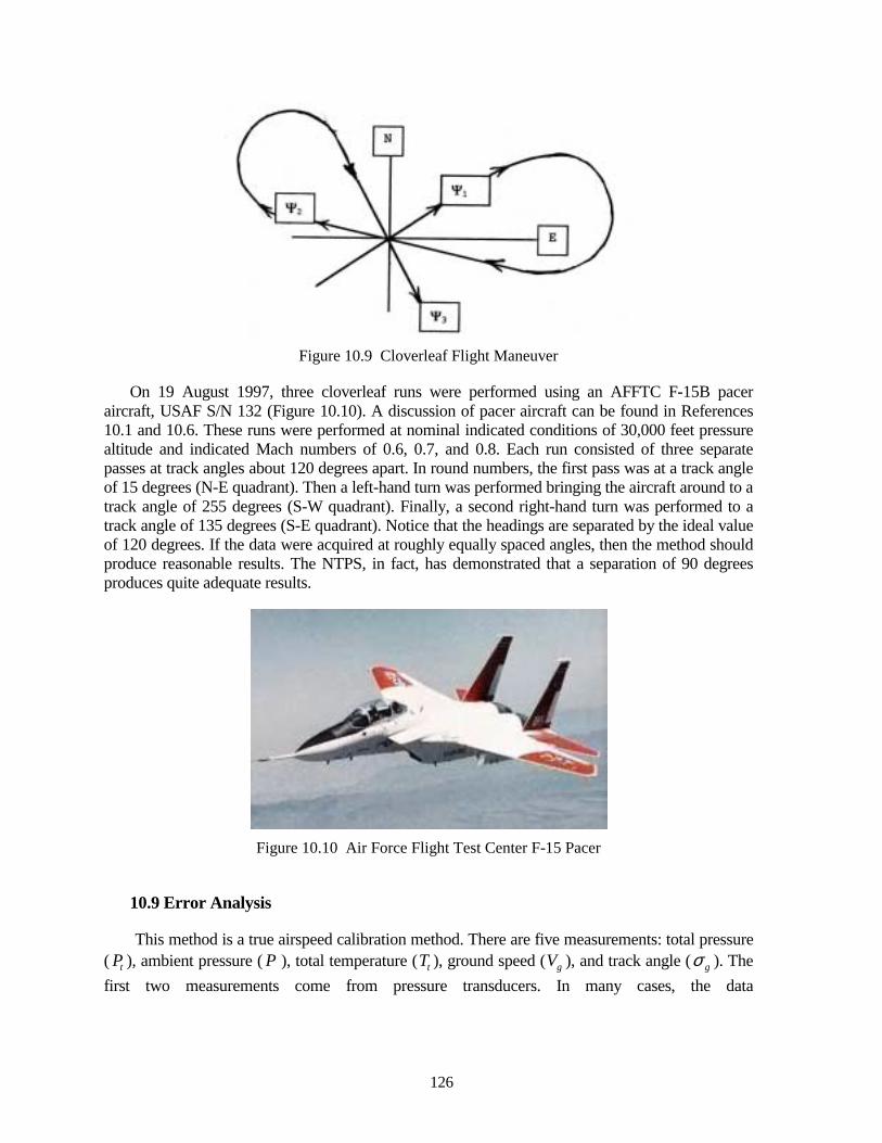
http://www.tycho.navy.mil/gpsinfo.html.(I

126

Figure 10.9 Cloverleaf Flight Maneuver

On 19 August 1997, three cloverleaf runs were performed using an AFFTC F-15B pacer aircraft, USAF S/N 132 (Figure 10.10). A discussion of pacer aircraft can be found in References 10.1 and 10.6. These runs were performed at nominal indicated conditions of 30,000 feet pressure altitude and indicated Mach numbers of 0.6, 0.7, and 0.8. Each run consisted of three separate passes at track angles about 120 degrees apart. In round numbers, the first pass was at a track angle of 15 degrees (N-E quadrant). Then a left-hand turn was performed bringing the aircraft around to a track angle of 255 degrees (S-W quadrant). Finally, a second right-hand turn was performed to a track angle of 135 degrees (S-E quadrant). Notice that the headings are separated by the ideal value of 120 degrees. If the data were acquired at roughly equally spaced angles, then the method should produce reasonable results. The NTPS, in fact, has demonstrated that a separation of 90 degrees produces quite adequate results.

Figure 10.10 Air Force Flight Test Center F-15 Pacer

10.9 Error Analysis

This method is a true airspeed calibration method. There are five measurements: total pressure ( tP ), ambient pressure ( P ), total temperature ( tT ), ground speed ( gV ), and track angle ( gσ ). The first two measurements come from pressure transducers. In many cases, the data

127

source may be altitude and airspeed. In that case, total and static pressure are computed from altitude and airspeed. The third one is from a total temperature probe. The last two parameters are either GPS or radar measurements. The laboratory calibration accuracy for pressure transducers is about ± 0.001 in. Hg (0.071 psf) and about ± 0.10 °K for temperature probes. Therefore, one will use these numbers and pick a typical condition near the test conditions of the data shown in this handbook.

a. Mach number = 0.800,

b. Pressure Altitude = 30,000 feet, and

c. Ambient Temperature = 242.0 °K.

At those conditions (and carrying out computations to beyond usual resolution):

a. tP = 957.944 psf,

b. aP = 628.432 psf,

c. tT = 272.98 °K, and

d. tV = 484.959 knots (true airspeed).

Since we are working with two different units on pressure, the conversion factor is as follows:

a. in. Hg = 70.726 psf

add 0.001 in. Hg "error" to tP

b. Pt = 958.0147

computing true airspeed

c. tV = 484.999 knots.

The error in computed true airspeed for an error in total pressure then is:

d. ( tV∆ )/( tP∆ ) = (484.999 - 484.959)/(958.0147-957.944) = 0.565 (knots/psf) = 0.044 knots per 0.001 in. Hg Total Pressure.

Hence, for the laboratory accuracy of 1-milli-inch of mercury (0.001 in. Hg) the error in total pressure results in a 0.044-knot error in true airspeed. Keep in mind this is the error slope at just this one set of conditions.

To examine ambient pressure errors, add the same error (0.001 in. Hg) to ambient pressure, while keeping the other parameters the same.

a. P = 628.5027,

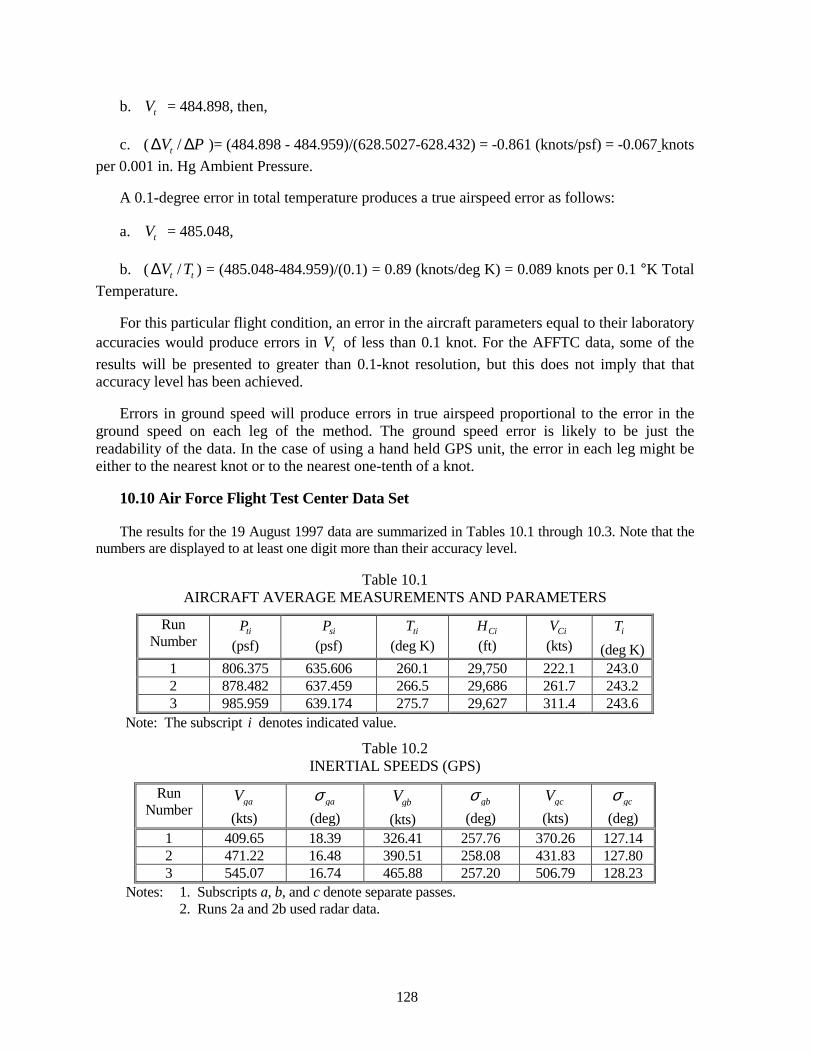
128

b. tV = 484.898, then,

c. ( /tV P∆ ∆ )= (484.898 - 484.959)/(628.5027-628.432) = -0.861 (knots/psf) = -0.067 knots per 0.001 in. Hg Ambient Pressure.

A 0.1-degree error in total temperature produces a true airspeed error as follows:

a. tV = 485.048,

b. ( /t tV T∆ ) = (485.048-484.959)/(0.1) = 0.89 (knots/deg K) = 0.089 knots per 0.1 °K Total Temperature.

For this particular flight condition, an error in the aircraft parameters equal to their laboratory accuracies would produce errors in tV of less than 0.1 knot. For the AFFTC data, some of the results will be presented to greater than 0.1-knot resolution, but this does not imply that that accuracy level has been achieved.

Errors in ground speed will produce errors in true airspeed proportional to the error in the ground speed on each leg of the method. The ground speed error is likely to be just the readability of the data. In the case of using a hand held GPS unit, the error in each leg might be either to the nearest knot or to the nearest one-tenth of a knot.

10.10 Air Force Flight Test Center Data Set

The results for the 19 August 1997 data are summarized in Tables 10.1 through 10.3. Note that the numbers are displayed to at least one digit more than their accuracy level.

Table 10.1 AIRCRAFT AVERAGE MEASUREMENTS AND PARAMETERS

Run Number

tiP (psf)

siP (psf)

tiT (deg K)

CiH (ft)

CiV (kts)

iT (deg K)

1 806.375 635.606 260.1 29,750 222.1 243.0 2 878.482 637.459 266.5 29,686 261.7 243.2 3 985.959 639.174 275.7 29,627 311.4 243.6

Note: The subscript i denotes indicated value.

Table 10.2 INERTIAL SPEEDS (GPS)

Run Number

gaV (kts)

gaσ (deg)

gbV (kts)

gbσ (deg)

gcV (kts)

gcσ (deg)

1 409.65 18.39 326.41 257.76 370.26 127.14 2 471.22 16.48 390.51 258.08 431.83 127.80 3 545.07 16.74 465.88 257.20 506.79 128.23

Notes: 1. Subscripts a, b, and c denote separate passes. 2. Runs 2a and 2b used radar data.

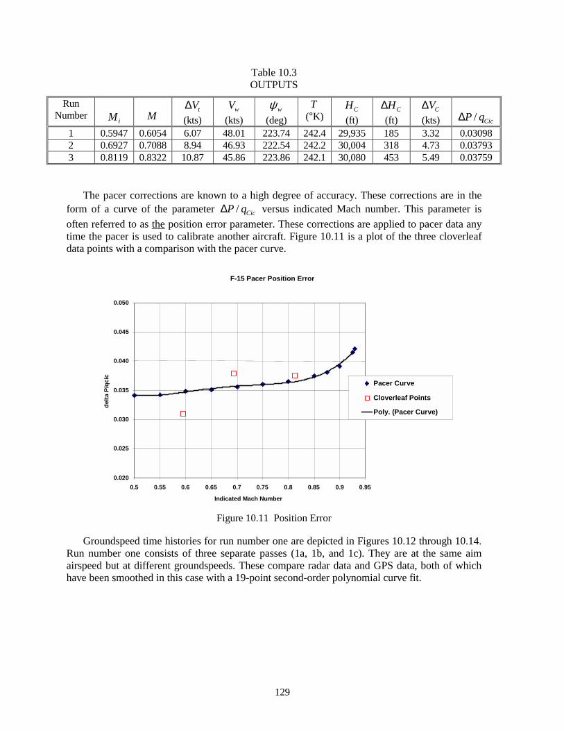
129

Table 10.3 OUTPUTS

Run Number

iM

M

tV∆ (kts)

wV (kts)

wψ (deg)

T (°K)

CH (ft)

CH∆ (ft)

CV∆ (kts)

/ CicP q∆

1 0.5947 0.6054 6.07 48.01 223.74 242.4 29,935 185 3.32 0.03098 2 0.6927 0.7088 8.94 46.93 222.54 242.2 30,004 318 4.73 0.03793 3 0.8119 0.8322 10.87 45.86 223.86 242.1 30,080 453 5.49 0.03759

The pacer corrections are known to a high degree of accuracy. These corrections are in the form of a curve of the parameter / CicP q∆ versus indicated Mach number. This parameter is often referred to as the position error parameter. These corrections are applied to pacer data any time the pacer is used to calibrate another aircraft. Figure 10.11 is a plot of the three cloverleaf data points with a comparison with the pacer curve.

F-15 Pacer Position Error

0.020

0.025

0.030

0.035

0.040

0.045

0.050

0.5 0.55 0.6 0.65 0.7 0.75 0.8 0.85 0.9 0.95

Indicated Mach Number

delta

P/q

cic

Pacer Curve

Cloverleaf Points

Poly. (Pacer Curve)

Figure 10.11 Position Error

Groundspeed time histories for run number one are depicted in Figures 10.12 through 10.14. Run number one consists of three separate passes (1a, 1b, and 1c). They are at the same aim airspeed but at different groundspeeds. These compare radar data and GPS data, both of which have been smoothed in this case with a 19-point second-order polynomial curve fit.

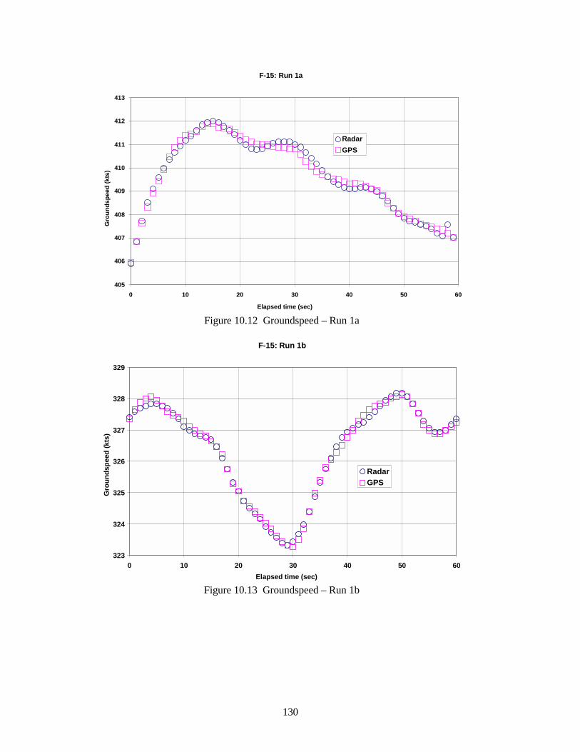
130

F-15: Run 1a

405

406

407

408

409

410

411

412

413

0 10 20 30 40 50 60

Elapsed time (sec)

Gro

unds

peed

(kts

)

RadarGPS

Figure 10.12 Groundspeed – Run 1a

F-15: Run 1b

323

324

325

326

327

328

329

0 10 20 30 40 50 60Elapsed time (sec)

Gro

unds

peed

(kts

)

RadarGPS

Figure 10.13 Groundspeed – Run 1b

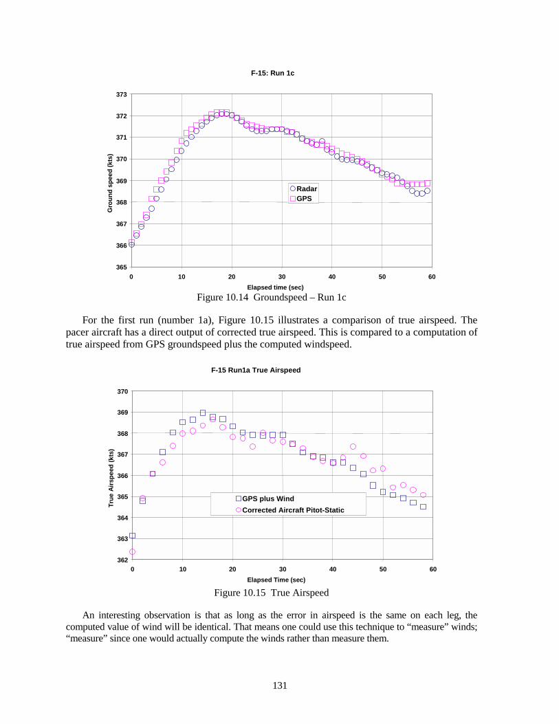
131

F-15: Run 1c

365

366

367

368

369

370

371

372

373

0 10 20 30 40 50 60Elapsed time (sec)

Gro

und

spee

d (k

ts)

RadarGPS

Figure 10.14 Groundspeed – Run 1c

For the first run (number 1a), Figure 10.15 illustrates a comparison of true airspeed. The pacer aircraft has a direct output of corrected true airspeed. This is compared to a computation of true airspeed from GPS groundspeed plus the computed windspeed.

F-15 Run1a True Airspeed

362

363

364

365

366

367

368

369

370

0 10 20 30 40 50 60Elapsed Time (sec)

True

Airs

peed

(kts

)

GPS plus WindCorrected Aircraft Pitot-Static

Figure 10.15 True Airspeed

An interesting observation is that as long as the error in airspeed is the same on each leg, the computed value of wind will be identical. That means one could use this technique to “measure” winds; “measure” since one would actually compute the winds rather than measure them.

132

From the start of the first pass (1a) to the completion of the last pass (3c) was 37 minutes. This was an excessive amount of time for these tests. It seems clear that something considerably less than a full minute of data on each pass would be quite adequate. A 10-second average would suffice. Then, by relaxing the requirement to maintain the test airspeed exactly, an additional amount of test time could be saved. Without the need for radar, tracking it becomes unnecessary to co-ordinate with the radar tracking team and that saves even more time. It seems reasonable that a factor of two or more savings in flight time could be achieved. Thus, not counting the time required to climb to the test altitude, each set of three passes could be concluded in about 5 minutes or less.

10.11 Mathematics of the Cloverleaf Method

The basic vector equation that one will solve for the cloverleaf method is nothing more than true airspeed equals the vector sum of groundspeed and windspeed.

t g wV V V= +" " "

(10.13)

tN gN wNV V V= + (10.14)

tE gE wEV V V= + (10.15)

t ti tV V V= + ∆ (10.16)

The north and east components of groundspeed are either direct outputs of the GPS or are computed as follows:

cos( )gN g gV V σ= ⋅ (10.17)

sin( )gE g gV V σ= ⋅ (10.18)

The aircraft track angle (or the direction of the groundspeed vector) is gσ . Writing down the relationship that true airspeed squared is equal to the sum of the squares of its components.

2 2 2t tN tEV V V= + (10.20)

Substituting equations 10.14 through 10.16 into equation 10.20 yields equation 10.21.

2 2 2( ) ( ) ( )ti t gN wN gE wEV V V V V V+ ∆ = + + + (10.21)

Multiplying out equation 10.21 and collecting terms, one gets:

(2 ) (2 )t ti t wN gN wNV V V V V V∆ ⋅ ⋅ + ∆ − ⋅ ⋅ +

2 2(2 ) ( )wE gE wE g tiV V V V V− ⋅ ⋅ + = − (10.22)

133

Defining the following:

a. tx V= ∆

b. wNy V=

c. wEz V=

d. 2 2g tiC V V= −

1 2 2ti t tiA V V V x= ⋅ + ∆ = ⋅ + (10.23)

2 2 2gN wN gNA V V V y= ⋅ + = ⋅ + (10.24)

3 2 2gE wE gEA V V V z= ⋅ + = ⋅ + (10.25)

Each pass produces an equation. As show in equation 10.26, subscript 1 is the first pass, 2 is the second, and 3 is the third. The unknowns , andx y z are presumed constant for all three runs. In matrix form, the equations are as follows:

1 1 1 1

2 2 2 2

3 3 3 3

1 2 31 2 31 2 3

A A A x CA A A y CA A A z C

− − − − ⋅ = − −

(10.26)

In matrix shorthand form:

[ ] { } { }A X C⋅ = (10.26)

The vector of unknowns { }X is solved by multiplying each side of equation 10.26 by the

inverse of the [ ]A matrix.

{ } [ ] { }1X A C−= ⋅ (10.27)

The unknowns , andx y z in the{ }X are also contained in [ ]A . So an iteration is required. The initial estimates for the X values will be zero. Then, the matrix equation is used to compute a new set of X values. These values are inserted into [ ]A , [ ]A is inverted again, and equation 10.27 is used again. Repeat the process until convergence occurs. When the iteration is complete you have solved for the desired numbers, namely an error in true airspeed and two components of wind.

134

SECTION 10 REFERENCES

10.1. Albert G. DeAnda, AFFTC Standard Airspeed Calibration Procedures, AFFTC-TIH-81-5, Air Force Flight Test Center, Edwards AFB, California, June 1981.

10.2 Olson, Wayne M. 1998. “Pitot-Static Calibration Using a GPS Multi-Track Method.” Paper

presented at the 29th Annual Symposium of the Society of Flight Test Engineers (SFTE), Reno, September 15.

10.3. Wayne M. Olson, “True Airspeed Calibration Using Three Radar Passes,” Performance and

Flying Qualities Branch Office Memo, Air Force Flight Test Center, Edwards AFB, California, August 1976.

10.4. J.A.Lawford and K.R.Nipress, “Calibration of Air Data Systems and Flow Direction Sensors,”

pages 16-20, AGARD AG-300-Vol.1, September 1983. 10.5. Gregory V. Lewis, “A Flight Test Technique Using GPS For Position Error Correction

Testing,” National Test Pilot School, Mojave, California, July 1997. 10.6. William Gracey, "Measurement of Aircraft Speed and Altitude,” John Wiley and Sons, 1981.

11.0 CRUISE

11.1 Introduction

Cruise performance is usually considered the most important test performed during the performance testing phase. Especially for transport and bomber aircraft since most of the fuel consumed during a typical mission is during stabilized cruise. For accurate mission planning, it is critical to be able to predict fuel consumption. Cruise testing was also the most time consuming test for transport and bomber aircraft. Even for fighter aircraft, it was a significant portion of the performance flight test program. The emphasis is on was, as efforts are being made to reduce the amount of flight time spent collecting cruise performance data.

The primary parameters in cruise performance are specific range ( SR ) and range factor ( RF ). Specific range is nautical air miles per pound of fuel used. Range factor is specific range multiplied by gross weight.

A typical cruise data point can take up to 10 minutes to perform. This is usually required for engine and aircraft stabilization. The typical stabilization requirement is an airspeed change of 1 knot per minute. This is equivalent to roughly 0.001 g in flight path acceleration, which is roughly 1 percent in drag or fuel flow. A simple example will show this 1-percent factor. For a transport category aircraft, a typical lift to drag ratio is an even 10.

a. / 10 / 0.10L D or D L= =

b. tL W≅ / 0.10tD W = 0.10 tD W= ⋅

c. n exD F F= −

d. 0.001xN = 0.001 tD W∆ = ⋅

e. 0.001 0.01 1.0%0.10

t

t

WD orD W

− ⋅∆ = = − −⋅

For non-afterburner operation, a 1-percent change in drag will equate to about a 1-percent change in fuel flow. We strive for an accuracy of 1 percent in cruise performance. There are many sources of error, which add up to this 1 percent. We have errors in gross weight, pressure altitude, Mach number, ambient temperature, fuel flow, and flight path acceleration. The main sources of error are in the last two: fuel flow and flight path acceleration. With modern instrumentation (as of the writing of this handbook), we have been achieving at least 1-percent uncertainty in fuel flow. With an INS, we have computed flight path acceleration ( xN ) to better than 0.001 g. By using INS data, we no longer have to spend 10 minutes to get the aircraft perfectly stabilized because we can accurately measure any small acceleration and make accurate corrections to the data. The other reason for 10-minute speed power points was to get the engine perfectly stabilized. During a series of cruise points, the pilot made only small throttle changes between points and kept the throttle fixed at near constant flight conditions for several minutes so very long stabilization periods should not be required with modern engines.

136

11.2 Cruise Tests

Cruise tests are done to determine aircraft range and endurance and to help in the development of drag, thrust, and fuel flow relationships. Cruise is a wings level, constant altitude, and constant speed maneuver. Testing is often accomplished by testing a matrix of constant aircraft gross weight-pressure ratio ( /tW δ ) points. The altitude is varied between points to yield an average /tW δ to be a specified value. It is, however, an approximation that constant /tW δ generalizes the data in any way. There are altitude effects on the data. The preferred method is to do constant altitude testing at varying gross weights to cover a range of /tW δ and altitude. The data could be corrected to nominal /tW δ values, but by correcting to weight and altitude it is easier to make flight manual comparisons. Table 11.1 represents B-52G data. The G model has turbojet engines that were 1950's vintage.

Table 11.1 B-52G CRUISE DATA

Altitude (ft)

Weight (lbs)

Specific Range (nm/lb)

Range Factor (nm)

35,000 400,017 0.0242 9,680 50,000 194,574 0.0437 8,503

Note: The cruise condition was 1.7 million pounds /tW δ and Mach number = 0.76.

The average degradation in range factor for the B-52G is 0.81 percent per 1,000 feet of altitude increase.

In the case of the B-52H model, the average degradation in range factor is 0.56 percent per 1,000 feet of altitude increase. Another data point is early F-16A data that indicated about a 0.50 percent per thousand-foot degradation factor. The F-16A is not a long-range aircraft and as such had a much smaller fuel fraction. Fuel fraction is the ratio of total fuel weight at engine start to empty gross weight.

Points are flown by stabilizing as nearly as possible to aim airspeed and altitude, typically ±0.01 Mach number and ±100 feet of altitude. The usual stabilization criterion is 1 knot per minute in airspeed and 50 feet per minute in altitude. With an INS to compute aircraft acceleration, the stabilization criterion could be relaxed somewhat. Typically, it takes up to 10 minutes to get the aircraft stabilized followed by 30 seconds to 1 minute of recorded data. Cruise testing is very time consuming with this method. By relaxing the stabilization criterion, considerable savings in time could be achieved. In addition, a real-time display of computed flight path acceleration could be useful in reducing the time required to stabilize.

11.3 Range

The computation of range ( R ) during cruise is the integration of true airspeed as follows:

tR V dt= ⋅∫ (11.1)

137

where:

dt = time increment (hours), and R = range (nam [nautical air miles]), 6,076.115 feet = 1 nm (1,852 meters, exactly).

We could put the range equation in different forms by making some substitutions. First, we want to put Mach number ( M ) into the equation by using the Mach number equation as detailed in the airspeed section of this handbook.

a. tVM a= , and

b. 661.48SLa a θ θ= ⋅ = ⋅ .

Substituting into the range equation.

( )661.48R M dtθ= ⋅ ⋅ ⋅∫ (11.2)

Defining fuel flow as the negative of the rate of change of weight:

tf

dWWdt

= −

(11.3)

where:

fW = fuel flow (pounds/hour), and

tdW = incremental weight (pounds).

1

tf

dt dWW

= − ⋅

(11.4)

Substituting for equation 11.4 into equation 11.2:

661.48t

f

MR dWW

θ ⋅ ⋅= − ⋅ ∫ (11.5)

Making these substitutions:

ff

WW δ θ

δ θ

= ⋅ ⋅ ⋅ (11.6)

/ tt

WWδ δ =

(11.7)

138

f tf

t

W WWW

θδ θ

δ

= ⋅ ⋅ ⋅

(11.8)

The integration is from a start weight ( tsW ) to an end weight ( teW ).

661.48te

ts

W

Wf t

t

MR dt

W WW

θ

θδ θ

δ

⋅ ⋅ = − ⋅ ⋅ ⋅ ⋅

∫ (11.9)

It’s not as bad as it looks. Canceling the θ terms and putting tW under dt :

( )

661.48te

ts

tW

tWf

WM dtRWW

δ

δ θ

⋅ ⋅ = − ⋅

⋅

∫ (11.10)

If one were to fly constant Mach number and maintain constant /tW δ , then the numerator term could be brought out of the integral. This would involve a slow cruise climb and we will show how much extra thrust that requires. At constant /tW δ and M , the lift coefficient would be a constant. Then, ignoring the change in skin friction drag with altitude, the drag coefficient will be constant. Ignoring the thrust component, drag coefficient (as derived in the lift and drag section) is as follows:

( )

2

/0.000675 n

D

FC

M Sδ

= ⋅⋅

(11.11)

Then /nF δ will be constant, since we have assumed that Mach number and DC are constant.

The corrected thrust specific fuel consumption relation is as follows:

( )

/

f

f

nn

W

Wtsfc

FF

δ θθ

θδ

⋅ = =

⋅

(11.12)

139

We have presumed the denominator ( /nF δ ) to be a constant. The /tsfc θ is also considered to be approximately a constant at constant Mach number and /nF δ . Now, we can pull these (approximately) constant terms out of the integral and integrate.

( )

661.48 te

ts

t W

tWf

WM dtRWW

δ

δ θ

⋅ ⋅ = −

⋅

∫ (11.13)

The term in front of the integral is called range factor ( RF ).

te

ts

W

tW

dtR RFW

= − ⋅ ∫ (11.14)

You may be more used to seeing RF in the following identical form:

tt t

f

VRF W SR WW

= ⋅ = ⋅ (nautical air miles) (11.15)

where:

SR = specific range (nautical air miles per pound of fuel).

From a table of integrals and natural logarithm relationships:

( ) ( )ln ln ln lnb

a

dx b ab a a bx= − = = −∫

where:

ln = natural logarithm.

ln ts

te

WR RFW

= ⋅

(11.16)

The above equation is convenient to get a quick estimate of range given only the average range factor and the start and end cruise weight. Note that this is the range during the cruise segment and does not include taxi, takeoff, climb, and descent.

11.4 Computing Range from Range Factor

Using the previous tabulated B-52G data, we will compute range and show the magnitude of the climb factor. We will assume that the two points at 35,000 and 50,000 feet are the beginning and end of the cruise segment of a mission. The cruise is at constant 0.77 Mach number and a

140

/tW δ of 1,700,000 pounds. Using previously defined formulas for true airspeed, energy altitude, and pressure ratio we construct Table 11.2. We will linearly interpolate versus altitude for range factor.

Table 11.2 RANGE FACTOR VERSUS ALTITUDE FOR B-52G

Altitude

(ft)

True Airspeed

(kts)

Energy Altitude

(ft)

Gross Weight

(lbs)

Net Thrust (lbs)

Range Factor (nm)

35,000 443.84 43,721 423,547 42,355 10,843 36,089 441.65 44,724 402,052 40,205 10,777 40,000 441.65 48,635 333,155 33,316 10,539 45,000 441.65 53,635 261,986 26,199 10,234 50,000 441.65 58,635 206,020 20,602 9,930

Note: Thrust was computed by assuming a lift to drag (L/D) ratio of 10. This is typical for a transport category aircraft.

We could get a first estimate of range by using an average range factor and the start and end conditions.

( )9,680 8,503 400,016ln ln 6,552 nam2 194,574

s

e

WR RFW

+ = ⋅ = ⋅ =

(11.17)

Since we assumed a linear variation of range factor with altitude, we will get the same result by integrating the individual segments. Range factor will not be a linear function of altitude, usually.

The time for this mission computes to be 54,100 seconds (15.04 hours). From the table, the delta energy altitude is 14,914 feet. The average speed is 736.5 feet per second. Now, we can calculate the average longitudinal load factor necessary to produce enough excess thrust to sustain this cruise climb.

( )( )14,91451,000 0.2955 0.00040736.5 745.6

Ex

t

HNV

= = = =!

(11.18)

At the average weight of 297,295 pounds, the average excess thrust calculates to 119 pounds. The average thrust is 29,730 pounds, therefore the ratio of excess thrust to net thrust is:

a. 119 0.0040 0.40%29,730

ex

n

F orF

= =

By ignoring the excess thrust, we over estimated the range by 26 nam (0.40 percent of 6,552 nam). Quite small, but not negligible. On an actual mission, the mission profile would be step climbs. For this example, you would start the cruise segment at 35,000 feet and fly constant

141

altitude until it was decided to climb to a new altitude. This might be in increments of 4,000 feet. When flying in civilian airspace, the altitudes are 4,000 feet apart.

11.5 Constant Altitude Method of Cruise Testing

The recommended method of doing cruise testing is the constant altitude method. The F-15 and F-16 projects used constant altitude method. The B-1B used constant altitude analysis method, though the points were flown using the constant weight/pressure ratio ( /tW δ ) method. The constant altitude method consists of choosing a range of weight and altitude conditions to cover the aircraft envelope and then flying each weight/altitude combination over a range of speeds. For an aircraft with a large weight fraction, this may mean flying up to six altitudes at up to three weights (heavy, mid, and light). This could mean a maximum of 18 weight/altitude combinations. Nevertheless, with a reasonable amount of thrust/drag/fuel flow analysis, this could be cut in half or more. Flying all three weights at the predicted optimum cruise /tW δ is usually desirable. The altitudes are chosen by selecting six evenly spaced /tW δ ’s from minimum to maximum with one at the predicted optimum. The minimum is based upon minimum weight at a minimum altitude and the maximum is based upon the cruise ceiling defined as a climb capability of 300 feet per minute. The altitudes are then rounded to the nearest 5,000 feet, which allows for easy flight manual comparisons since flight manuals typically have cruise charts at even 5,000-foot increments.

For ease of flight manual comparisons, the data presented in reports are a specific range, or range factor versus Mach number at even 5,000-foot increments for standard weights, representing rounded values of heavy, mid, and light gross weight.

11.6 Range Mission

Range missions are performed to gain confidence in the performance data collected during climb, cruise, and descent. Rather than relying on fuel flow measurements and thrust/drag analysis, the primary measurement during a range mission is aircraft fuel quantity indications. The mission is performed by climbing to a given start cruise altitude, progressively stepping up in the altitude during constant altitude/Mach number cruise segments, and finally doing an idle power descent. Total fuel used is obtained from the fuel quantity system. A calibration of the fuel quantity system is obtained during the aircraft empty weight and fuel calibration. Using a performance simulation, the test day mission performance could be estimated. The simulation thrust/drag/fuel relationships were previously determined using data from several maneuvers including climb, cruise, and descent. The simulation estimates of fuel used were compared with measured fuel used during the mission.

A practical reality of the flight test programs was that it was difficult to justify devoting an entire sortie to only a range mission. A compromise was to obtain fuel-used data during long cruise segments that often occurred during certain systems tests. During the B-1B project, fuel used data were acquired from several training sorties flown on production aircraft at Dyess AFB, Texas. The data came from constant airspeed/altitude segments of several hours in duration. A comparison of fuel used was made with simulation results. The differences were well within the often-quoted 3-percent accuracy for performance data. This provided a valuable confirmation of the flight test results.

142

11.7 Slow Accel-Decel

A supplement, or perhaps even an alternative to cruise testing, is to do slow accels and decels. The data are used to build or verify a thrust versus fuel flow model. In addition, the data could be standardized to zero excess thrust. The maneuvers are flown sufficiently slowly to make the maximum correction to a range factor of about 10 percent. This compared with 1-percent corrections made to cruise data. We could estimate the zero excess thrust range factor from both the accel maneuver and the decel maneuver. The average of the accel and decel standardized range factors is a good estimate of zero excess thrust range factor since relatively small corrections are being made.

The maneuver is done at a rate of less than 1 knot per 3 seconds to yield an accel/decel rate of about 20 times the cruise stabilization criterion. A typical accel/decel maneuver takes about 6 to 12 minutes. The throttle is moved in small increments during the run to keep the accel/decel rate small, but not so small that the maneuver would take too long, thereby losing the advantage over stabilized cruise. If the cruise tests are done with a relaxed stabilization criterion (±100 feet and ±2 knots in 20 seconds) with only 20 seconds of recorded data, then the dynamic cruise has an advantage over the slow accel-decel data. If it is desired to collect, thrust and fuel flow data over a range of conditions then the slow accel-decel is a good approach.

11.8 Effect of Wind on Range

The typical high altitude cruise for both fighter and transport aircraft is about 0.85 Mach number. The true airspeed for standard day in the lower atmosphere (troposphere) and upper atmosphere (stratosphere) can be computed using formulas from the airspeed section. For standard day from 11 kilometers (36,089 feet) to 20 kilometers (65,617 feet), the temperature is 216.65 degrees K.

a. 216.65661.48 0.85 487.5288.15tV = ⋅ ⋅ = knots

The formula for specific range (nams per pound of fuel) is just true airspeed ( tV ) over fuel flow ( fW ).

t

f

VSR W= (11.19)

We can compute a specific range with respect to the ground as follows:

gg

f

VSR W= (11.20)

Since groundspeed equals true airspeed minus wind and taking just the component parallel to the direction of flight (track angle):

t g wV V V= + (11.21)

143

( )t wg

f

V VSR W−= (11.22)

Finally, the ratio of specific range with respect to the ground to the specific range with respect to the moving air mass (equation 11.22 divided by equation 11.19) is as follows:

( )g t w

t

SR V VSR V

−= (11.23)

As shown in Appendix A, windspeed at an ambient pressure of 200 millibars (mb) (38,661 feet) averages about 40 knots above Edwards AFB. The average direction is about 215 degrees (S-W). Since wind direction is the direction from which the wind is blowing, an aircraft heading of 215 degrees would have a 40-knot headwind for this average Edwards wind. A headwind is a positive wind. For this condition, the range degradation would be:

a. ( )487.5 40 0.918 8.2 percent487.5gSR

SR−= = = degradation

This is for an average wind if one were heading directly into the wind. A set of data collected for the cloverleaf paper (a portion of which is in the cloverleaf subsection of the air data system calibration section) had winds in excess of excess of 100 knots. This data were not included in this handbook, but was AFFTC data set number 2 in the referenced paper (Reference 10.2). In addition, the wind data shown Appendix A indicates a standard deviation of about 25 knots. Flying directly into a 100-knot wind would produce the following specific range degradation:

a. ( )487.5 100 0.795 20.5 percent487.5gSR

SR−= = = degradation

One could just as easily be flying with that wind as a tailwind.

a. ( )487.5 100 1.205 20.5 percent487.5gSR

SR+= = = improvement

In general, you would only be affected by the component of wind parallel to the flight direction. Wind vector relationships are discussed in detail Section 10.11. This wind effect is only relevant in computing physical (ground) nautical miles with a given wind. When collecting cruise data, you are flying with respect to the moving air mass.

144

12.0 ACCELERATION AND CLIMB

12.1 Acceleration

Accelerations are conducted for multiple purposes. First, to determine optimum climb schedules by observing the peak of specific excess power versus Mach number. The actual optimum occurs to the right of the peak of specific excess power ( sP ) versus M curves, depending on whether it is desirable to achieve a minimum time to climb or minimum fuel for fixed range. Second, to determine the obvious acceleration performance, i.e., fuel used, time, and distance to accelerate. Third, to determine drag/thrust/fuel flow models. Climb data can be used for this purpose also, however, accelerations are a more efficient method. The accelerations are conducted over a range of altitudes.

The acceleration maneuver is performed wings level, 1-g, and fixed throttle at constant altitude. Usually a climb or turn is done at the beginning of the run to get the engine thermally stabilized. Then the aircraft accelerates to a point where the acceleration rate is reduced to a small value (less than 1 knot per 10 seconds). The altitude is maintained constant during the run. Indicated altitude will jump as the aircraft passes through the transonic speed regime. Thus, it is necessary to maintain zero flight path angle usually by maintaining pitch attitude (θ ). Once through the transonic jump, an indicated altitude could be used for the rest of the acceleration. Modern aircraft with a head-up display (HUD) and INS have a velocity vector displayed on the HUD. Level flight through the transonic region is obtained by maintaining the velocity vector on the horizon.

Figure 12.1 is a sample of some actual acceleration data. The data points have been corrected to standard conditions. Standard conditions consist of standard weight, pressure altitude, and standard day atmospheric conditions. The fairing is the result of modeling thrust and drag, then computing specific excess power from thrust and drag. With one relatively short maneuver, one obtains a range of speed (Mach number) at a given altitude. By performing accelerations at various altitudes, climb performance can be computed. However, a few continuous climbs need to be conducted to confirm that performance (time, distance, and fuel used) computed from accelerations yields the same result as that from climbs. Accelerations are also performed at elevated g levels. These are discussed in the turn section.

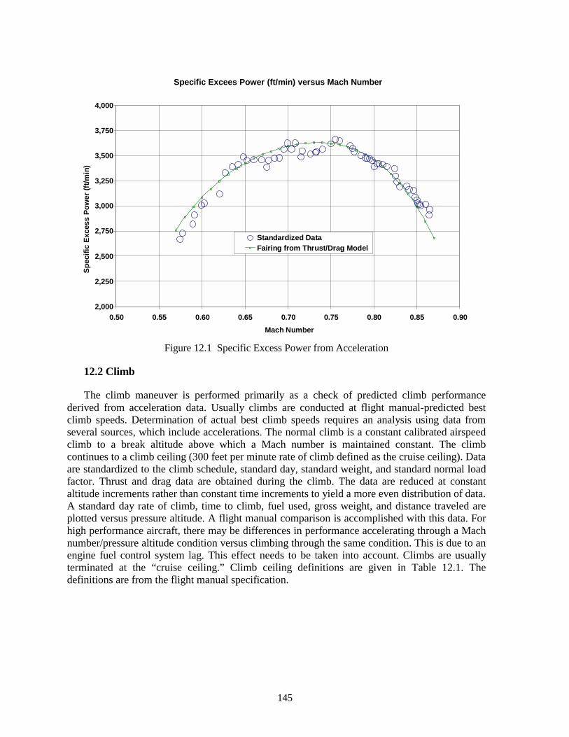
145

Specific Excees Power (ft/min) versus Mach Number

2,000

2,250

2,500

2,750

3,000

3,250

3,500

3,750

4,000

0.50 0.55 0.60 0.65 0.70 0.75 0.80 0.85 0.90Mach Number

Spec

ific

Exce

ss P

ower

(ft/m

in)

Standardized DataFairing from Thrust/Drag Model

Figure 12.1 Specific Excess Power from Acceleration

12.2 Climb

The climb maneuver is performed primarily as a check of predicted climb performance derived from acceleration data. Usually climbs are conducted at flight manual-predicted best climb speeds. Determination of actual best climb speeds requires an analysis using data from several sources, which include accelerations. The normal climb is a constant calibrated airspeed climb to a break altitude above which a Mach number is maintained constant. The climb continues to a climb ceiling (300 feet per minute rate of climb defined as the cruise ceiling). Data are standardized to the climb schedule, standard day, standard weight, and standard normal load factor. Thrust and drag data are obtained during the climb. The data are reduced at constant altitude increments rather than constant time increments to yield a more even distribution of data. A standard day rate of climb, time to climb, fuel used, gross weight, and distance traveled are plotted versus pressure altitude. A flight manual comparison is accomplished with this data. For high performance aircraft, there may be differences in performance accelerating through a Mach number/pressure altitude condition versus climbing through the same condition. This is due to an engine fuel control system lag. This effect needs to be taken into account. Climbs are usually terminated at the “cruise ceiling.” Climb ceiling definitions are given in Table 12.1. The definitions are from the flight manual specification.

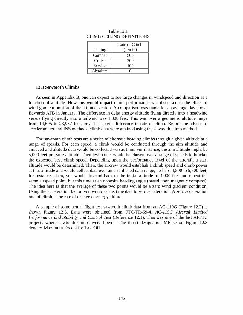
146

Table 12.1 CLIMB CEILING DEFINITIONS

Ceiling

Rate of Climb (ft/min)

Combat 500 Cruise 300 Service 100

Absolute 0

12.3 Sawtooth Climbs

As seen in Appendix B, one can expect to see large changes in windspeed and direction as a function of altitude. How this would impact climb performance was discussed in the effect of wind gradient portion of the altitude section. A comparison was made for an average day above Edwards AFB in January. The difference in delta energy altitude flying directly into a headwind versus flying directly into a tailwind was 1,308 feet. This was over a geometric altitude range from 14,605 to 23,937 feet, or a 14-percent difference in rate of climb. Before the advent of accelerometer and INS methods, climb data were attained using the sawtooth climb method.

The sawtooth climb tests are a series of alternate heading climbs through a given altitude at a range of speeds. For each speed, a climb would be conducted through the aim altitude and airspeed and altitude data would be collected versus time. For instance, the aim altitude might be 5,000 feet pressure altitude. Then test points would be chosen over a range of speeds to bracket the expected best climb speed. Depending upon the performance level of the aircraft, a start altitude would be determined. Then, the aircrew would establish a climb speed and climb power at that altitude and would collect data over an established data range, perhaps 4,500 to 5,500 feet, for instance. Then, you would descend back to the initial altitude of 4,000 feet and repeat the same airspeed point, but this time at an opposite heading angle (based upon magnetic compass). The idea here is that the average of these two points would be a zero wind gradient condition. Using the acceleration factor, you would correct the data to zero acceleration. A zero acceleration rate of climb is the rate of change of energy altitude.

A sample of some actual flight test sawtooth climb data from an AC-119G (Figure 12.2) is shown Figure 12.3. Data were obtained from FTC-TR-69-4, AC-119G Aircraft Limited Performance and Stability and Control Test (Reference 12.1). This was one of the last AFFTC projects where sawtooth climbs were flown. The thrust designation METO on Figure 12.3 denotes Maximum Except for TakeOff.

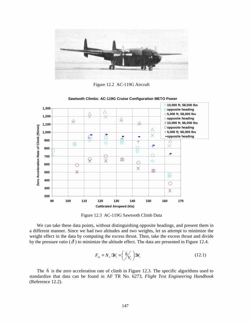
147

Figure 12.2 AC-119G Aircraft

Sawtooth Climbs: AC-119G Cruise Configuration METO Power

200

300

400

500

600

700

800

900

1,000

1,100

1,200

1,300


Zero

Acc

eler

atio

n R

ate

of C

limb

(ft/m

in)

10,000 ft; 58,000 lbsopposite heading5,000 ft; 58,000 lbsopposite heading10,000 ft; 66,000 lbsopposite heading5,000 ft; 66,000 lbsopposite heading

Figure 12.3 AC-119G Sawtooth Climb Data

We can take these data points, without distinguishing opposite headings, and present them in a different manner. Since we had two altitudes and two weights, let us attempt to minimize the weight effect in the data by computing the excess thrust. Then, take the excess thrust and divide by the pressure ratio (δ ) to minimize the altitude effect. The data are presented in Figure 12.4.

ex x t tt

hF N W WV = ⋅ = ⋅ ! (12.1)

The h! is the zero acceleration rate of climb in Figure 12.3. The specific algorithms used to standardize that data can be found in AF TR No. 6273, Flight Test Engineering Handbook (Reference 12.2).

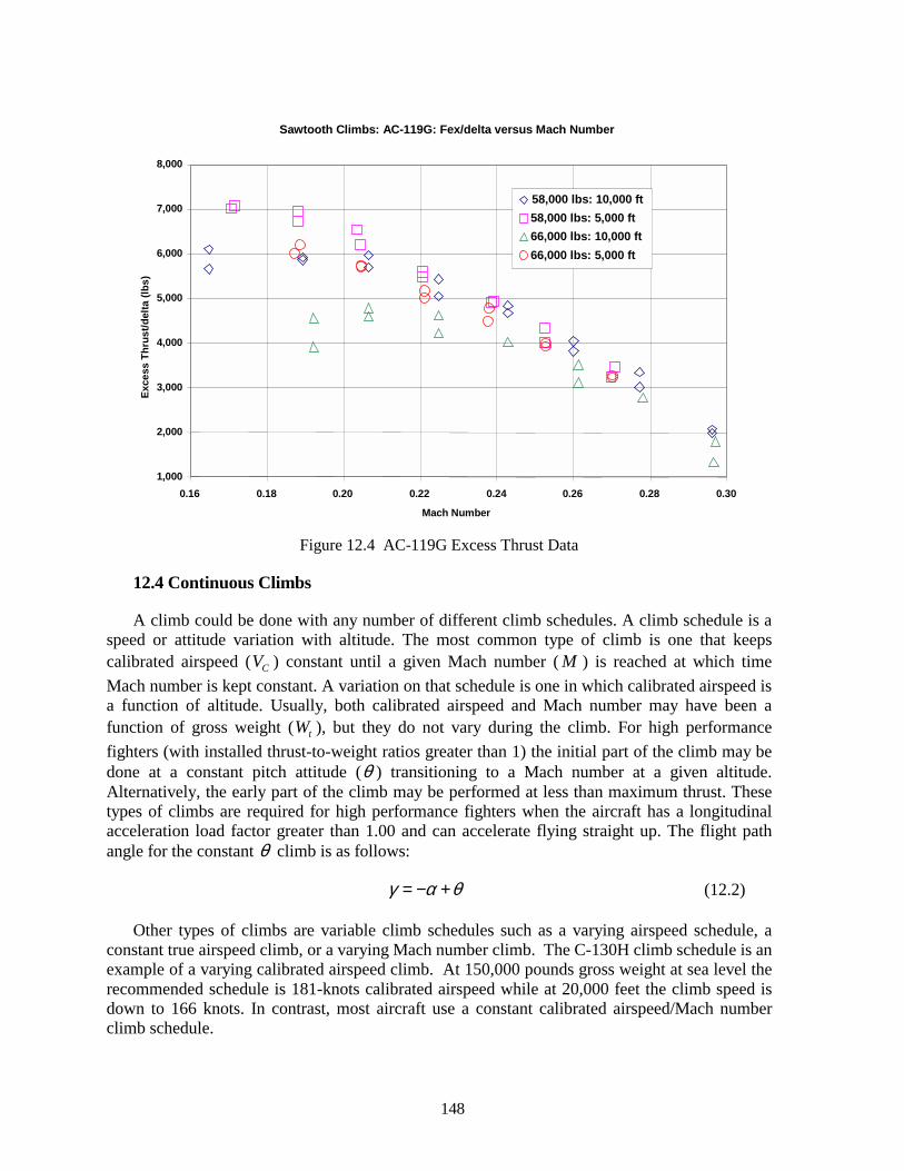
148

Sawtooth Climbs: AC-119G: Fex/delta versus Mach Number

1,000

2,000

3,000

4,000

5,000

6,000

7,000

8,000

0.16 0.18 0.20 0.22 0.24 0.26 0.28 0.30

Mach Number

Exce

ss T

hrus

t/del

ta (l

bs)

58,000 lbs: 10,000 ft58,000 lbs: 5,000 ft66,000 lbs: 10,000 ft66,000 lbs: 5,000 ft

Figure 12.4 AC-119G Excess Thrust Data

12.4 Continuous Climbs

A climb could be done with any number of different climb schedules. A climb schedule is a speed or attitude variation with altitude. The most common type of climb is one that keeps calibrated airspeed ( CV ) constant until a given Mach number ( M ) is reached at which time Mach number is kept constant. A variation on that schedule is one in which calibrated airspeed is a function of altitude. Usually, both calibrated airspeed and Mach number may have been a function of gross weight ( tW ), but they do not vary during the climb. For high performance fighters (with installed thrust-to-weight ratios greater than 1) the initial part of the climb may be done at a constant pitch attitude (θ ) transitioning to a Mach number at a given altitude. Alternatively, the early part of the climb may be performed at less than maximum thrust. These types of climbs are required for high performance fighters when the aircraft has a longitudinal acceleration load factor greater than 1.00 and can accelerate flying straight up. The flight path angle for the constant θ climb is as follows:

γ α θ= − + (12.2)

Other types of climbs are variable climb schedules such as a varying airspeed schedule, a constant true airspeed climb, or a varying Mach number climb. The C-130H climb schedule is an example of a varying calibrated airspeed climb. At 150,000 pounds gross weight at sea level the recommended schedule is 181-knots calibrated airspeed while at 20,000 feet the climb speed is down to 166 knots. In contrast, most aircraft use a constant calibrated airspeed/Mach number climb schedule.

149

Accelerations and climbs are both fixed throttle maneuvers. They are usually done with power settings like MIL or MAX. Decelerations and descents are usually done in power settings such as IDLE, though there could have been a MIL power deceleration under certain conditions such as supersonic.

12.5 Climb Parameters

/R C H= !

0

1 t tV dVAFg dH

= + ⋅

(12.3)

where:

/R C = rate of climb (ft/sec), and AF = acceleration factor.

12.6 Acceleration Factor (AF)

The acceleration factor ( AF ) is used in climb performance as a simple conversion between a rate of change of tapeline or geopotential altitude and rate of change of energy altitude.

a. EHAFH

=!!

Most aircraft climbs are conducted by either holding calibrated airspeed ( CV ) or Mach ( M ) number constant. In reality, the calibrated airspeed or Mach number is not exactly constant but let us make some calculations assuming that they are held exactly constant and that there is zero wind so that true airspeed ( tV ) and inertial speeds ( gV ) are identical. The true airspeed vector defines the flight path (or wind) axis. The component of aircraft acceleration parallel to the flight path is the longitudinal acceleration ( xA ). The longitudinal load factor ( xN ) is simply the xA divided by the acceleration of gravity ( 0g ). In conventional aircraft performance, g is assumed a constant at the reference gravity and given the value of 32.174 ft/sec². Figure 12.5 is a representation of acceleration factor for climb at constant calibrated airspeed.

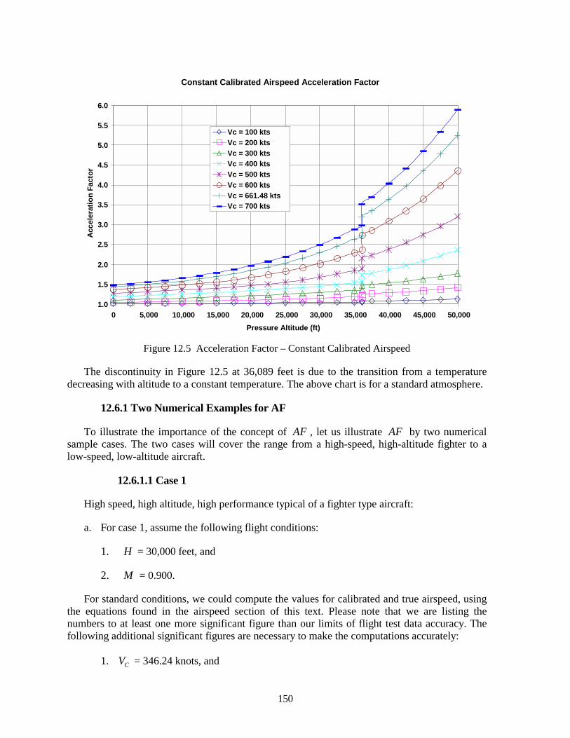
150

Constant Calibrated Airspeed Acceleration Factor

1.0

1.5

2.0

2.5

3.0

3.5

4.0

4.5

5.0

5.5

6.0

0 5,000 10,000 15,000 20,000 25,000 30,000 35,000 40,000 45,000 50,000Pressure Altitude (ft)

Acc

eler

atio

n Fa

ctor

Vc = 100 ktsVc = 200 ktsVc = 300 ktsVc = 400 ktsVc = 500 ktsVc = 600 ktsVc = 661.48 ktsVc = 700 kts

Figure 12.5 Acceleration Factor – Constant Calibrated Airspeed

The discontinuity in Figure 12.5 at 36,089 feet is due to the transition from a temperature decreasing with altitude to a constant temperature. The above chart is for a standard atmosphere.

12.6.1 Two Numerical Examples for AF

To illustrate the importance of the concept of AF , let us illustrate AF by two numerical sample cases. The two cases will cover the range from a high-speed, high-altitude fighter to a low-speed, low-altitude aircraft.

12.6.1.1 Case 1

High speed, high altitude, high performance typical of a fighter type aircraft:

a. For case 1, assume the following flight conditions:

1. H = 30,000 feet, and

2. M = 0.900.

For standard conditions, we could compute the values for calibrated and true airspeed, using the equations found in the airspeed section of this text. Please note that we are listing the numbers to at least one more significant figure than our limits of flight test data accuracy. The following additional significant figures are necessary to make the computations accurately:

1. CV = 346.24 knots, and

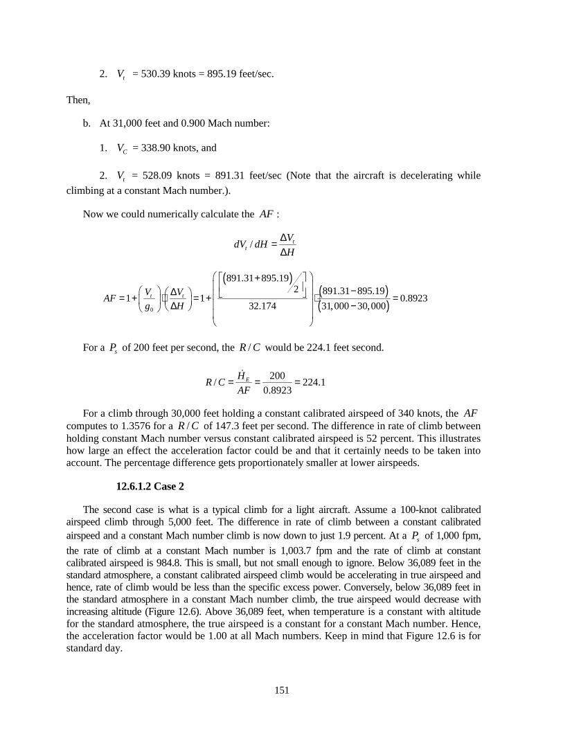
151

2. tV = 530.39 knots = 895.19 feet/sec.

Then,

b. At 31,000 feet and 0.900 Mach number:

1. CV = 338.90 knots, and

2. tV = 528.09 knots = 891.31 feet/sec (Note that the aircraft is decelerating while climbing at a constant Mach number.).

Now we could numerically calculate the AF :

/ tt

VdV dHH

∆=∆

( )

( )( )0

891.31 895.192 891.31 895.19

1 1 0.892332.174 31,000 30,000

t tV VAFg H

+ − ∆ = + ⋅ = + ⋅ = ∆ −

For a sP of 200 feet per second, the /R C would be 224.1 feet second.

200/ 224.10.8923

EHR CAF

= = =!

For a climb through 30,000 feet holding a constant calibrated airspeed of 340 knots, the AF computes to 1.3576 for a /R C of 147.3 feet per second. The difference in rate of climb between holding constant Mach number versus constant calibrated airspeed is 52 percent. This illustrates how large an effect the acceleration factor could be and that it certainly needs to be taken into account. The percentage difference gets proportionately smaller at lower airspeeds.

12.6.1.2 Case 2

The second case is what is a typical climb for a light aircraft. Assume a 100-knot calibrated airspeed climb through 5,000 feet. The difference in rate of climb between a constant calibrated airspeed and a constant Mach number climb is now down to just 1.9 percent. At a sP of 1,000 fpm, the rate of climb at a constant Mach number is 1,003.7 fpm and the rate of climb at constant calibrated airspeed is 984.8. This is small, but not small enough to ignore. Below 36,089 feet in the standard atmosphere, a constant calibrated airspeed climb would be accelerating in true airspeed and hence, rate of climb would be less than the specific excess power. Conversely, below 36,089 feet in the standard atmosphere in a constant Mach number climb, the true airspeed would decrease with increasing altitude (Figure 12.6). Above 36,089 feet, when temperature is a constant with altitude for the standard atmosphere, the true airspeed is a constant for a constant Mach number. Hence, the acceleration factor would be 1.00 at all Mach numbers. Keep in mind that Figure 12.6 is for standard day.

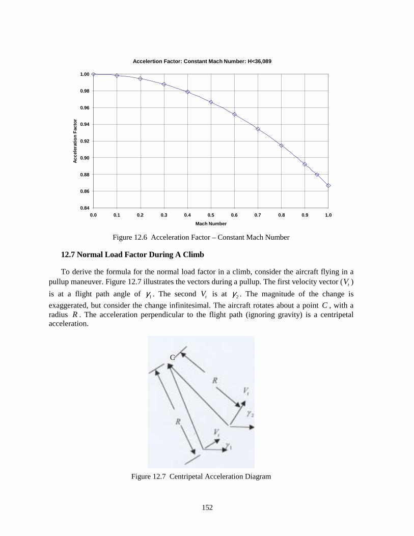
Accelertion Factor: Constant Mach Number: H<36,089

0.84

0.86

0.88

0.90

0.92

0.94

0.96

0.98

1.00

0.0 0.1 0.2 0.3 0.4 0.5 0.6 0.7 0.8 0.9 1.0

Mach Number

Acce

lera

tion

Fact

or

Figure 12.6 Acceleration Factor – Constant Mach Number

12.7 Normal Load Factor During A Climb

To derive the formula for the normal load factor in a climb, consider the aircraft flying in a pullup maneuver. Figure 12.7 illustrates the vectors during a pullup. The first velocity vector ( tV ) is at a flight path angle of 1γ . The second tV is at 2γ . The magnitude of the change is exaggerated, but consider the change infinitesimal. The aircraft rotates about a point C , with a radius R . The acceleration perpendicular to the flight path (ignoring gravity) is a centripetal acceleration.

Figure 12.7

C

152

Centripetal Acceleration Diagram

153

The centripetal acceleration is as follows:

2

tVaR

= (12.4)

The radius is related to the linear velocity through the angular velocity (ω ).

tV Rω= ⋅ (12.5)

The angular velocity ω is just the derivative of the flight path angle.

( )( )

2 1

2 1

ddt t t t

γ γγ γω γ−∆= = = =∆ −! (12.6)

Solving for the radius R in equation 12.5 and substituting into the acceleration equation 12.4:

2

tt

t

Va VV

γ

γ

= = ⋅

!

!

(12.7)

Adding in the component of gravity yields:

0 cos ta g Vγ γ= ⋅ + ⋅ ! (12.8)

Finally, dividing by 0g yields the load factor in the normal axis.

0

cos tz

VNgγγ ⋅= +!

(12.9)

The above equations are valid for constant winds. Usually, the load factors are computed from INS velocities and angles plus true airspeed to enable a transformation from the inertial axis to the flight path axis. What is desired are inertial accelerations in the wind (or flight path) axis. Therefore, if the aircraft has an INS, and the appropriate software to do the axis transformations, then there is no need to be concerned about horizontal winds and wind gradients. In addition, the difference between a tapeline rate of climb and pressure altitude rate of climb is taken into account, since the INS yields geometric rate of climb. The INS data is, however, sensitive to the presence of any vertical winds, so efforts are made to fly in areas where no vertical winds are expected. For Edwards AFB, the best place to conduct performance tests is over the ocean. Both the B-1B and C-17A aircraft conducted their entire cruise testing over the ocean.

12.8 Descent

A typical descent schedule is a constant Mach number intersecting a constant calibrated airspeed. The data are used to generate descent performance, an idle thrust map, and drag polar information to complete the performance model. The performance model is used to check

154

mission performance. The idle power descent could be accomplished with speed brakes extended.

12.9 Deceleration

Decelerations are conducted to provide data to compute descent performance. A deceleration is performed by accelerating to the Mach number limit then moving the throttle to idle and conducting a wings level, constant altitude deceleration. This maneuver gives us idle thrust versus speed. Due to inaccuracies in the in-flight thrust deck, there could be a drag difference at idle thrust versus drag polar data acquired at higher power settings. The same maneuver could be accomplished with the speed brakes extended.

SECTION 12.0 REFERENCES

12.1 Pape, James K. and McDowell, Edward D., AC-119G Aircraft Limited Performance and Stability and Control Tests, FTC-TR-69-4, AFFTC, Edwards AFB, California, March 1969.

12.2 Herrington, Russel M., et al, Flight Test Engineering Handbook, AF TR 6273, AFFTC, Edwards AFB, California, revised January 1966.

155

13.0 TURNING

13.1 Introduction

Turning performance is defined as flight at other than 1 g, usually in the horizontal plane. There are four different types of turns: accelerating or decelerating, thrust-limited, stabilized, and lift-limited.

13.2 Accelerating or Decelerating Turns

Accelerating or decelerating turns are performed at a fixed throttle, constant g, and constant altitude. For accelerating turns, the maneuver is done by starting fast, applying specified throttle, and pulling into a turn to decelerate the aircraft. Next, reduce g level to the specified value and accelerate to either the specified Mach number or the maximum speed. The data acquired could be used to generate energy maneuverability charts or to contribute to the aircraft drag, thrust, and fuel flow model.

Turns at fixed g, constant altitude, and fixed throttle are referred to as accelerating or decelerating turns. Turns, in general, are used to quantify the turning performance capability of the aircraft and to help in the development of the drag and lift curves. With the advent of dynamic performance, fewer turns are conducted in flight test. Turns are used primarily to check the performance model created from 1-g acceleration and dynamic performance maneuvers. Nevertheless, some turns are still necessary as confidence builders in the model and to demonstrate specification performance.

13.3 Thrust-Limited Turns

A thrust-limited turn is a turn where the pilot attempts to maintain throttle setting, Mach number, and pressure altitude while varying normal load factor. Usually about 30 seconds or 180 degrees of turn data are recorded at stabilized conditions; however, maintaining stabilized conditions is often difficult. The data are used to verify the thrust/drag model for sustained g and to assist in the development of the drag and lift curves. The data are collected at a stabilized g and as such, may be of higher quality than data from dynamic maneuvers. Nevertheless, keep in mind that the thrust-limited turn is dynamic since it is at elevated g values (and large pitch rates) and may be at different power settings than the dynamic performance data. There may have been throttle effects on the drag polar due to inaccuracies in the in-flight thrust computation. One value of thrust-limited turns is it produces thrust data that is stabilized while accelerations and decelerations are dynamic in thrust. So, the lag time constant for thrust could be estimated. With fuel controls scheduling on total temperature in the inlet, there may be a different lag constant depending on whether the aircraft is climbing or accelerating through a point. The thrust-limited turn is stabilized at a given Mach number and pressure altitude condition. As with accelerating or decelerating turns, only a limited number of sustained or thrust-limited turns are performed because they are very fuel and time-consuming tests compared with the more efficient dynamic maneuvers. It is still necessary to perform a limited number of turns as checks on the model. It has been necessary on past projects to do significant numbers of turns because of disagreements between turn data and dynamic data on the drag polar. Developing correlation factors to adjust the drag polars to match the measured turn performance may be necessary. Not relying completely upon data obtained from dynamic performance maneuvers is important.

156

Using an INS for flight path accelerations requires a 1-g level run be accomplished before the turn to get a wind calibration. This applies to all turning maneuvers. Winds are computed from the wind calibration maneuver assuming zero sideslip. These winds are assumed to remain constant during the turn. The thrust and fuel flow data obtained in climbs and acceleration is dynamic and subject to engine and instrumentation lag. It is possible to attain lag time constants by comparing thrust-limited turn data to climb and acceleration data.

13.4 Stabilized Turns

Stabilized turns are turns where Mach number, pressure altitude, and normal load factor are specified and throttle is varied to obtain a stabilized condition. These maneuvers are useful to obtain lift and drag data at specific points along the drag and lift curves and to check for specification compliance. The flight test objective is to determine if such conditions can be achieved in stabilized flight at something less than or equal to maximum throttle. Another way to evaluate that spec point would be to do a thrust-limited turn at MAX thrust at the specified flight conditions and then determine whether the desired normal load factor in stabilized flight is achieved. Specs are usually written for standard day at a standard weight, center of gravity, etc. Therefore, you must correct the data to standard conditions to determine spec compliance since the spec may have been missed on the test day but the aircraft would have achieved the spec on a more favorable standard day. For the stabilized turn, you would have needed some specialized software to perform the standardization or the turn could have been standardized assuming it is an accelerating turn at a given pressure altitude, Mach number, and normal load factor, then determine the flight path acceleration for standard conditions. If the longitudinal flight path load factor ( xN ) was positive for the given spec conditions, then the spec condition was met.

13.5 Lift-Limited Turns

When it is desired to determine limit performance at the angle-of-attack (α ) limit or the normal load factor ( zN ) limit then a lift-limited turn is performed. If the aircraft has an α/g limiter, as is the case on the F-16, then the turn is a full aft stick maneuver. Otherwise, the pilot must observe the flight manual limits, which makes this maneuver very difficult to fly without exceeding aircraft limits. The angle-of-attack limited portion of the maneuver is used to quantify the lift coefficient at the limit angle of attack and to check the angle-of-attack calibration at the limit. The check of angle of attack is performed with INS data. This maneuver produces data at the highest limits of the drag polar and the lift curve. You also obtain limited angle-of-attack data from a split-s. The split-s maneuver is discussed in the dynamic performance section.

Lift-limit and g-limit turns are accomplished by accelerating to limit speed then pulling into a maximum allowable g turn and allowing the aircraft to decelerate to the lift limit. This defines the lift limit and g limit performance. The throttle setting is usually MIL or MAX, but the maneuver may be done at any power setting. Besides getting limit performance, drag polar data at or near maximum lift coefficient are obtained.

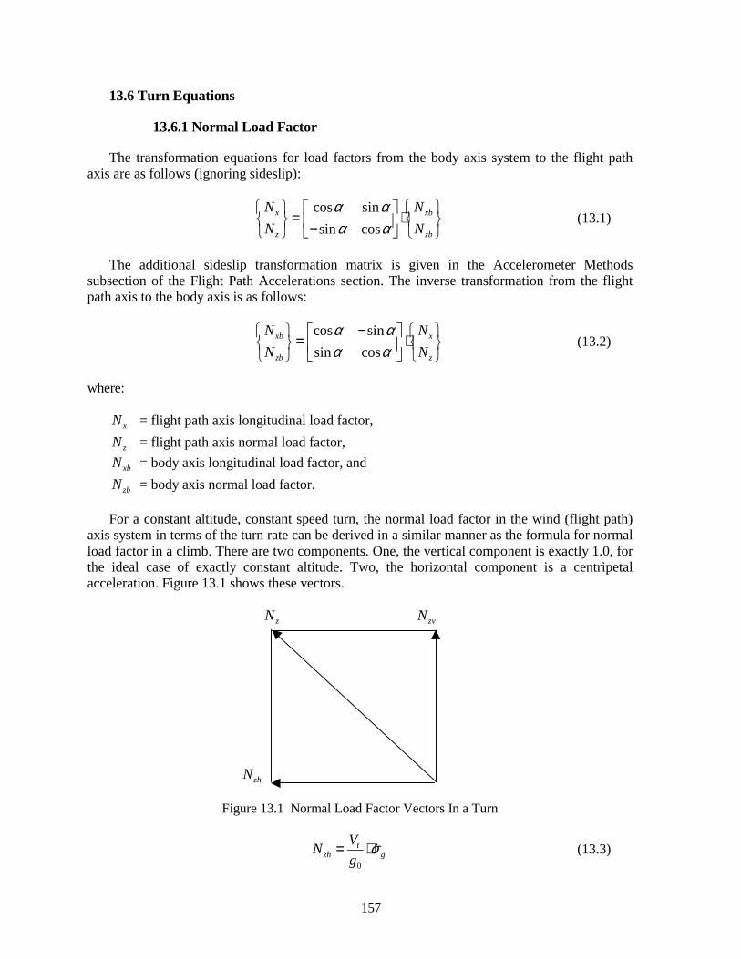
157

13.6 Turn Equations

13.6.1 Normal Load Factor

The transformation equations for load factors from the body axis system to the flight path axis are as follows (ignoring sideslip):

cos sinsin cos

xbx

zbz

NNNN

α αα α

= ⋅ −

(13.1)

The additional sideslip transformation matrix is given in the Accelerometer Methods subsection of the Flight Path Accelerations section. The inverse transformation from the flight path axis to the body axis is as follows:

cos sinsin cos

xb x

zb z

N NN N

α αα α

− = ⋅

(13.2)

where:

xN = flight path axis longitudinal load factor,

zN = flight path axis normal load factor,

xbN = body axis longitudinal load factor, and

zbN = body axis normal load factor.

For a constant altitude, constant speed turn, the normal load factor in the wind (flight path) axis system in terms of the turn rate can be derived in a similar manner as the formula for normal load factor in a climb. There are two components. One, the vertical component is exactly 1.0, for the ideal case of exactly constant altitude. Two, the horizontal component is a centripetal acceleration. Figure 13.1 shows these vectors.

zN zvN

zhN

Figure 13.1 Normal Load Factor Vectors In a Turn

0

tzh g

VNg

σ= ⋅ ! (13.3)

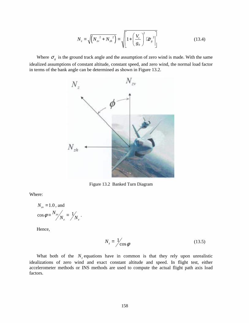
158

( )2

2 2 2

0

1 tz zv zh g

VN N Ng

σ = + = + ⋅

! (13.4)

Where gσ is the ground track angle and the assumption of zero wind is made. With the same idealized assumptions of constant altitude, constant speed, and zero wind, the normal load factor in terms of the bank angle can be determined as shown in Figure 13.2.

Figure 13.2 Banked Turn Diagram

Where:

1.0zvN = , and

1cos zv

z z

NN Nφ = = .

Hence,

1coszN φ= (13.5)

What both of the zN equations have in common is that they rely upon unrealistic idealizations of zero wind and exact constant altitude and speed. In flight test, either accelerometer methods or INS methods are used to compute the actual flight path axis load factors.

159

13.6.2 Turn Radius

In a steady, level turn the centripetal acceleration is the horizontal component of normal acceleration. The vertical component is 1-g; just the right amount to maintain exactly constant altitude for this idealized relationship.

2

tzh

VAR

= (feet/sec2) (13.6)

where:

R = turn radius (ft), tV = true airspeed (ft/sec), and

zhA = horizontal component of normal acceleration (ft/sec2).

From trigonometry:

( )2 1zh zN N= − (13.7)

and,

0

zhzh

AN g= (13.8)

Substituting equations 13.7 and equations 13.8 into equations 13.6 and solving for R :

a. ( ) ( )

2 2

2 20 1 32.174 1

t t

z z

V VRg N N

= =⋅ − ⋅ −

For R in feet and tV in knots:

( ) ( )

2

2

2 2

1.6878

32.174 1 91.653 1

t

t

z z

VVR

N N

= =

⋅ − ⋅ − (13.9)

13.7 Turn Rate

Once the turn radius is determined (equation 13.9), we can compute the turn rate. The relationship derives from the kinematics of constant speed rotation about a point.

tV Rω= ⋅ (13.10)

where:

160

R = radius of turn, and ω = turn rate.

The symbology we previously used for turn rate was σ! ; the rate of change of ground track angle. Then, solving for turn rate:

a. tg

VRσ =!

The above equation is valid for units of R in feet, tV in feet per second and gσ! in radians

per second. For R in feet, tV in knots and gσ! in degrees per second we get:

( )1.6878

57.2958 33.947t

tg

VV

RRσ

= ⋅ = ⋅

! (13.11)

13.8 Winds Aloft

Since the advent of the INS in the 1970s, it has been possible to compute accurate values of air data parameters in dynamic maneuvers such as turns. However, this required the use of wind calibration runs conducted in wings-level 1-g flight where the air data system errors were known from conventional tests. In addition, INS data had small drift errors in the groundspeeds. With the availability of the GPS in the 1990s, an accurate value of groundspeed was available. The mathematics and illustrating data for one such technique used in turning flight (that does not require the use of a wind calibration) will be presented.

The INS gives you six parameters of interest for performance and flying qualities. These are three angles called Euler angles and three velocities in the north ( N ), east ( E ) and down ( D ) directions. The Euler angles are the heading from true north designated psi (ψ ), the roll (or bank) angle designated phi (φ ), and the pitch attitude designated theta (θ ). The groundspeed components from an INS are gNV , gEV , and gDV . The problem is that we assumed we knew the groundspeeds accurately. We didn’t! The typical drift rate of an INS was on the order of 1 nautical mile per hour. Therefore, we had typical errors of about 1 knot in the horizontal groundspeeds at any one time. Now (late 1990s) we have a new device designated as embedded GPS/INS (EGI). This combines the outputs of an INS with the velocities and position data from the GPS using a filter. The GPS specification accuracies for the horizontal speeds are 0.1 m/sec (0.19 knot). This small error does not drift with time. Therefore, we have introduced a new level of accuracy into our data. Now, we will proceed to develop the equations starting with the basic vector relationship of true airspeed, groundspeed, and wind.

t g wV V V= +" " "

(13.12)

Solving for the magnitude of the true airspeed vector:

( ) ( ) ( )2 2 2

ti t gN wN gE wE gD wDV V V V V V V V + ∆ = + + + + + (13.13)

161

We will assume the vertical wind is zero. Taking the square of both sides:

( ) ( ) ( )2 22 2ti t gN wN gE wE gDV V V V V V V + ∆ = + + + +

(13.14)

From here on in the derivation, we will simply strive to minimize the sum of the difference between the left and right side of the above equation. Defining a parameter we shall call F* (F – star), we want to minimize the sum of this parameter simultaneously with respect to each of the three unknowns ( wNV , wEV , tV∆ ). The iteration is the method of Taylor’s series in three dimensions:

( )2 2 2 2* 0.5 tx ty tz tF V V V V= ⋅ + + − (13.15)

The 0.5 factor is just to eliminate ½ factors in the final formulation.

tx gN wNV V V= + (13.16)

ty gE wEV V V= + (13.17)

tz gDV V= (13.18)

t ti tV V V= + ∆ (13.19)

Defining three more parameters: ,f g and h :

*

1

N

i txi

f F V=

= ⋅∑ (13.20)

*

1

N

i tyi

g F V=

= ⋅∑ (13.21)

*

1

N

i ti

h F V=

= ⋅∑ (13.22)

There are N data points and N must be at least three. The , ,x y z unknowns are as follows:

a. wNx V= ,

b. wEy V= , and

c. tz V= ∆ .

We will assume zero initial estimates for the unknowns.

162

a. 0x y z= = =

In addition, initialize , ,f g h and the partial derivatives to zero as follows:

a. 0f g h= = = ,

b. / / / 0f x f y f z∂ ∂ = ∂ ∂ = ∂ ∂ = ,

c. / / / 0g x g y g z∂ ∂ = ∂ ∂ = ∂ ∂ = , and

d. / / / 0h x h y h z∂ ∂ = ∂ ∂ = ∂ ∂ = ,

Next we will generate a matrix of partial derivatives of ,f g and h . Summing from one to N :

( )2 *

1/

N

txi

f x V F=

∂ ∂ = + ∑ (13.23)

( ) ( )1

/ ( ) ( )N

ty txi

f y V i V i=

∂ ∂ = ⋅ ∑ (13.24)

( ) ( )1

/ ( ) ( )N

t txi

f z V i V i=

∂ ∂ = − ⋅ ∑ (13.25)

( ) ( )1

/ ( ) ( )N

tx tyi

g x V i V i=

∂ ∂ = ⋅ ∑ (13.26)

( )2 *

1/ ( )

N

tyi

g y V i F=

∂ ∂ = + ∑ (13.27)

( ) ( )1

/ ( ) ( )N

t tyi

g z V i V i=

∂ ∂ = − ⋅ ∑ (13.28)

( ) ( )1

/ ( ) ( )N

tx ti

h x V i V i=

∂ ∂ = ⋅ ∑ (13.29)

( ) ( )1

/ ( ) ( )N

ty ti

h y V i V i=

∂ ∂ = ⋅ ∑ (13.30)

( )2 *

1/ ( )

N

ti

h z V i F=

∂ ∂ = − + ∑ (13.31)

The following matrix formulation will solve for improved values for the unknowns:

163

1

1

/ / // / // / /

wN wN

wE wE

t tj j

V V f x g x h x fV V f y g y h y g

V V f z g z h z h

−

+

∂ ∂ ∂ ∂ ∂ ∂ = − ∂ ∂ ∂ ∂ ∂ ∂ ⋅ ∆ ∆ ∂ ∂ ∂ ∂ ∂ ∂ −

(13.32)

With improved values for the unknowns, simply return to the beginning of the algorithm and repeat the process until convergence occurs. This will usually occur after just a few steps. The parameter j is the iteration number. We now have the north and east components of wind and the previously unknown error in true airspeed.

14.0 DYNAMIC PERFORMANCE

14.1 Introduction

Dynamic performance typically involves the collection of lift and drag data at near constant Mach number with maneuvers that last less than 15 seconds. This is accomplished by varying normal load factor ( zN ) in a short time period. There are three dynamic performance maneuvers: roller coaster, split-s, and windup turn.

14.2 Roller Coaster

The roller coaster is a smooth sinusoidal variation of load factor versus time. The maneuver begins with a stabilized trimmed point at an aim Mach number, altitude ( CH ), and zN = 1.0. The throttle is kept constant during the maneuver. The maneuver is also called a pushover-pullup because that is what is done. The maneuver begins with a pushover to a g level less than 1.0. On fighter aircraft that is usually to an zN of 0.0 and on transport aircraft that is usually to an zN of 0.5. Then a pullup is performed back through zN of 1.0 to an zN of 1.5 on transport aircraft, or 2.0 or more on fighter aircraft. Some fighter projects used a maximum zN of more than 2.0 and some have used an aim angle of attack (α ) instead of a maximum load factor as the maximum point in the roller coaster. This maximum α is usually (but not always) something less than the limit α . This is because a large maximum α would produce large Mach number losses during the maneuver because the aircraft is at a high drag condition at a positive flight path angle (γ ) and is decelerating very rapidly. After attaining maximum zN then a pushover is performed back to zN = 1.0.

The rate of change of zN is between 0.25 and 0.50 g per second. The slower rate would produce larger Mach number variations but would also produce smaller rate effects on the data. Both Mach number and rate corrections are made to the data; therefore, the maneuver will take an average of 8 seconds to perform. Generally, there is a net altitude loss during the maneuver and a net Mach number loss, but both are quite small. The Mach number loss is usually no more than 0.01 and the altitude loss is less than 1,000 feet. If zN is more than 2.0 during the pullup, then the Mach number loss could be more than 0.01, but corrections are made to the data to nominal Mach numbers. Nominal Mach numbers would typically be 0.70, 0.80, 0.85, 0.90, etc.

A simulation of a roller coaster maneuver was conducted. The aircraft drag model was the same as for the takeoff simulation presented in the takeoff section. This was for a pseudo F-16 aircraft. For a lift coefficient less than 0.6 and low Mach numbers where compressibility is not substantial, Figure 14.1 represents the drag polar used.

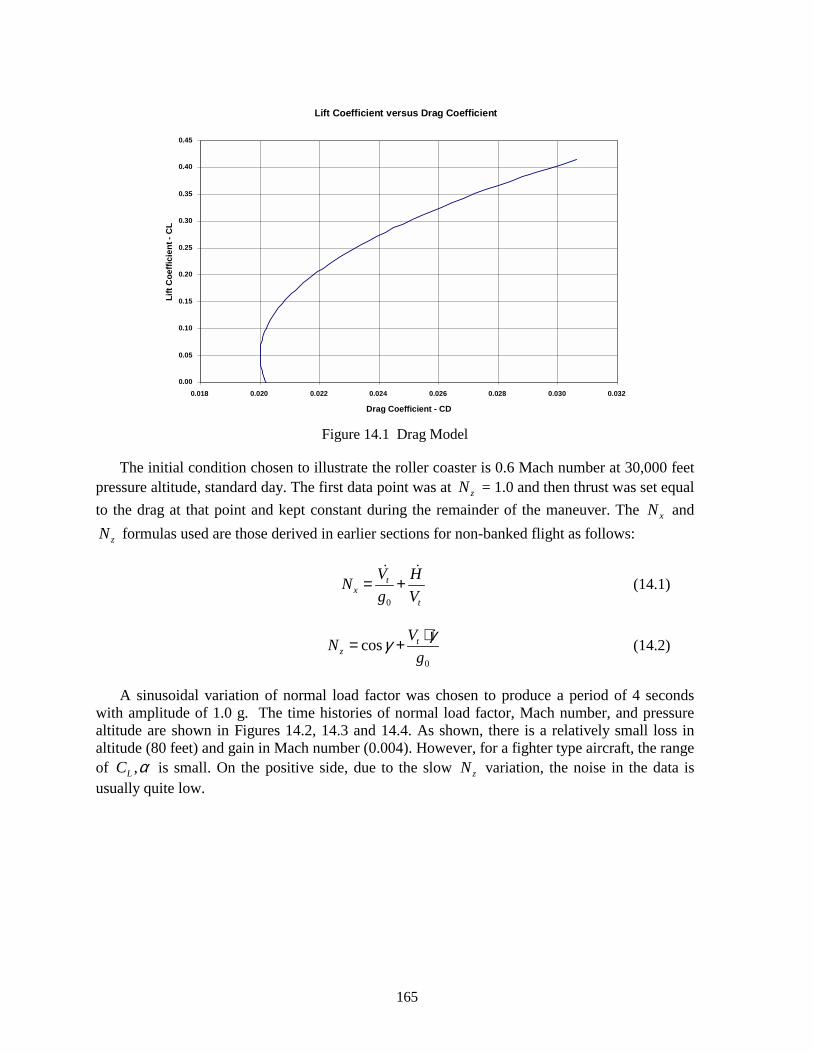
165

Lift Coefficient versus Drag Coefficient

0.00

0.05

0.10

0.15

0.20

0.25

0.30

0.35

0.40

0.45

0.018 0.020 0.022 0.024 0.026 0.028 0.030 0.032

Drag Coefficient - CD

Lift

Coe

ffici

ent -

CL

Figure 14.1 Drag Model

The initial condition chosen to illustrate the roller coaster is 0.6 Mach number at 30,000 feet pressure altitude, standard day. The first data point was at zN = 1.0 and then thrust was set equal to the drag at that point and kept constant during the remainder of the maneuver. The xN and

zN formulas used are those derived in earlier sections for non-banked flight as follows:

0

tx

t

V HNg V

= +! !

(14.1)

0

cos tz

VNgγγ ⋅= +!

(14.2)

A sinusoidal variation of normal load factor was chosen to produce a period of 4 seconds with amplitude of 1.0 g. The time histories of normal load factor, Mach number, and pressure altitude are shown in Figures 14.2, 14.3 and 14.4. As shown, there is a relatively small loss in altitude (80 feet) and gain in Mach number (0.004). However, for a fighter type aircraft, the range of ,LC α is small. On the positive side, due to the slow zN variation, the noise in the data is usually quite low.

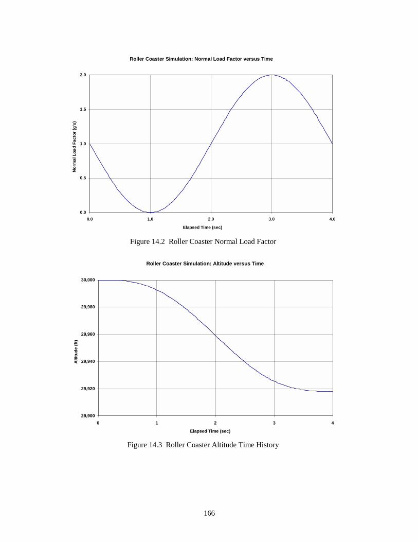
166

Roller Coaster Simulation: Normal Load Factor versus Time

0.0

0.5

1.0

1.5

2.0

0.0 1.0 2.0 3.0 4.0

Elapsed Time (sec)

Nor

mal

Loa

d Fa

ctor

(g's

)

Figure 14.2 Roller Coaster Normal Load Factor

Roller Coaster Simulation: Altitude versus Time

29,900

29,920

29,940

29,960

29,980

30,000

0 1 2 3 4

Elapsed Time (sec)

Alti

tude

(ft)

Figure 14.3 Roller Coaster Altitude Time History

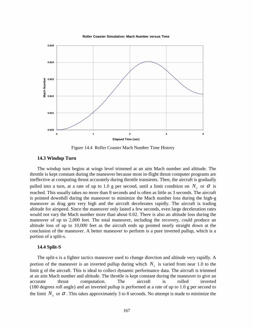
167

Roller Coaster Simulation: Mach Number versus Time

0.600

0.601

0.602

0.603

0.604

0.605

0 1 2 3 4

Elapsed Time (sec)

Mac

h N

umbe

r

Figure 14.4 Roller Coaster Mach Number Time History

14.3 Windup Turn

The windup turn begins at wings level trimmed at an aim Mach number and altitude. The throttle is kept constant during the maneuver because most in-flight thrust computer programs are ineffective at computing thrust accurately during throttle transients. Then, the aircraft is gradually pulled into a turn, at a rate of up to 1.0 g per second, until a limit condition on zN or α is reached. This usually takes no more than 8 seconds and is often as little as 3 seconds. The aircraft is pointed downhill during the maneuver to minimize the Mach number loss during the high-g maneuver as drag gets very high and the aircraft decelerates rapidly. The aircraft is trading altitude for airspeed. Since the maneuver only lasted a few seconds, even large deceleration rates would not vary the Mach number more than about 0.02. There is also an altitude loss during the maneuver of up to 2,000 feet. The total maneuver, including the recovery, could produce an altitude loss of up to 10,000 feet as the aircraft ends up pointed nearly straight down at the conclusion of the maneuver. A better maneuver to perform is a pure inverted pullup, which is a portion of a split-s.

14.4 Split-S

The split-s is a fighter tactics maneuver used to change direction and altitude very rapidly. A portion of the maneuver is an inverted pullup during which zN is varied from near 1.0 to the limit g of the aircraft. This is ideal to collect dynamic performance data. The aircraft is trimmed at an aim Mach number and altitude. The throttle is kept constant during the maneuver to give an accurate thrust computation. The aircraft is rolled inverted (180 degrees roll angle) and an inverted pullup is performed at a rate of up to 1.0 g per second to the limit zN or α . This takes approximately 3 to 8 seconds. No attempt is made to minimize the

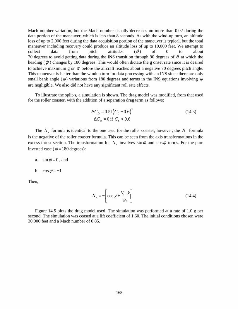
168

Mach number variation, but the Mach number usually decreases no more than 0.02 during the data portion of the maneuver, which is less than 8 seconds. As with the wind-up turn, an altitude loss of up to 2,000 feet during the data acquisition portion of the maneuver is typical, but the total maneuver including recovery could produce an altitude loss of up to 10,000 feet. We attempt to collect data from pitch attitudes (θ ) of 0 to about 70 degrees to avoid getting data during the INS transition through 90 degrees of θ at which the heading (ψ ) changes by 180 degrees. This would often dictate the g onset rate since it is desired to achieve maximum g or α before the aircraft reaches about a negative 70 degrees pitch angle. This maneuver is better than the windup turn for data processing with an INS since there are only small bank angle (φ ) variations from 180 degrees and terms in the INS equations involving φ are negligible. We also did not have any significant roll rate effects.

To illustrate the split-s, a simulation is shown. The drag model was modified, from that used for the roller coaster, with the addition of a separation drag term as follows:

( )20.5 0.6D LC C∆ = ⋅ − (14.3) 0 if 0.6D LC C∆ = <

The xN formula is identical to the one used for the roller coaster; however, the zN formula is the negative of the roller coaster formula. This can be seen from the axis transformations in the excess thrust section. The transformation for zN involves sinφ and cosφ terms. For the pure inverted case ( 180φ = degrees):

a. sin 0φ = , and

b. cos 1φ = − .

Then,

0

cos tz

VNgγγ

⋅= − +

! (14.4)

Figure 14.5 plots the drag model used. The simulation was performed at a rate of 1.0 g per second. The simulation was ceased at a lift coefficient of 1.60. The initial conditions chosen were 30,000 feet and a Mach number of 0.85.

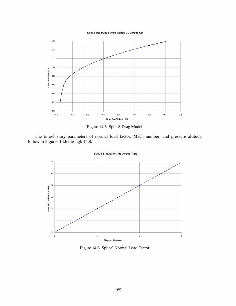
169

Split-s and Pullup Drag Model: CL versus CD

0.0

0.2

0.4

0.6

0.8

1.0

1.2

1.4

1.6

0.0 0.1 0.2 0.3 0.4 0.5 0.6 0.7 0.8

Drag Coefficient - CD

Lift

Coe

ffici

ent -

CL

Figure 14.5 Split-S Drag Model

The time-history parameters of normal load factor, Mach number, and pressure altitude follow in Figures 14.6 through 14.8.

Split-S Simulation: Nz versus Time

1

2

3

4

5

6

7

0 1 2 3

Elapsed Time (sec)

Nor

mal

Loa

d Fa

ctor

(Nz)

Figure 14.6 Split-S Normal Load Factor

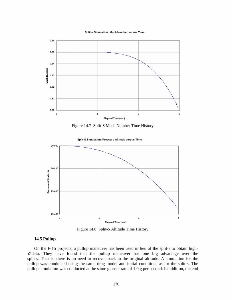
170

Split-s Simulation: Mach Number versus Time

0.80

0.81

0.82

0.83

0.84

0.85

0.86

0 1 2 3

Elapsed Time (sec)

Mac

h N

umbe

r

Figure 14.7 Split-S Mach Number Time History

Split-S Simulation: Pressure Altitude versus Time

29,400

29,600

29,800

30,000

0 1 2 3

Elapsed Time (sec)

Pres

sure

Alti

tude

(ft)

Figure 14.8 Split-S Altitude Time History

14.5 Pullup

On the F-15 projects, a pullup maneuver has been used in lieu of the split-s to obtain high-α data. They have found that the pullup maneuver has one big advantage over the split-s. That is, there is no need to recover back to the original altitude. A simulation for the pullup was conducted using the same drag model and initial conditions as for the split-s. The pullup simulation was conducted at the same g onset rate of 1.0 g per second. In addition, the end

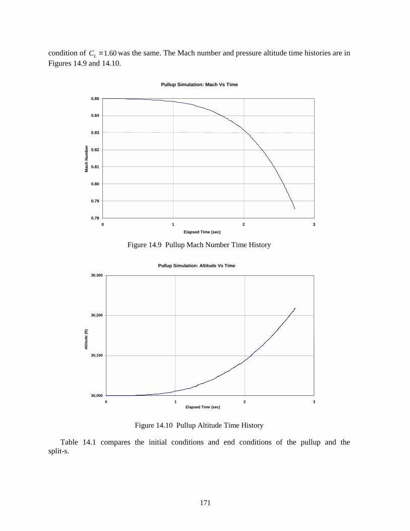
171

condition of 1.60LC = was the same. The Mach number and pressure altitude time histories are in Figures 14.9 and 14.10.

Pullup Simulation: Mach Vs Time

0.78

0.79

0.80

0.81

0.82

0.83

0.84

0.85

0 1 2 3

Elapsed Time (sec)

Mac

h N

umbe

r

Figure 14.9 Pullup Mach Number Time History

Pullup Simulation: Altitude Vs Time

30,000

30,100

30,200

30,300

0 1 2 3Elapsed Time (sec)

Altit

ude

(ft)

Figure 14.10 Pullup Altitude Time History

Table 14.1 compares the initial conditions and end conditions of the pullup and the split-s.

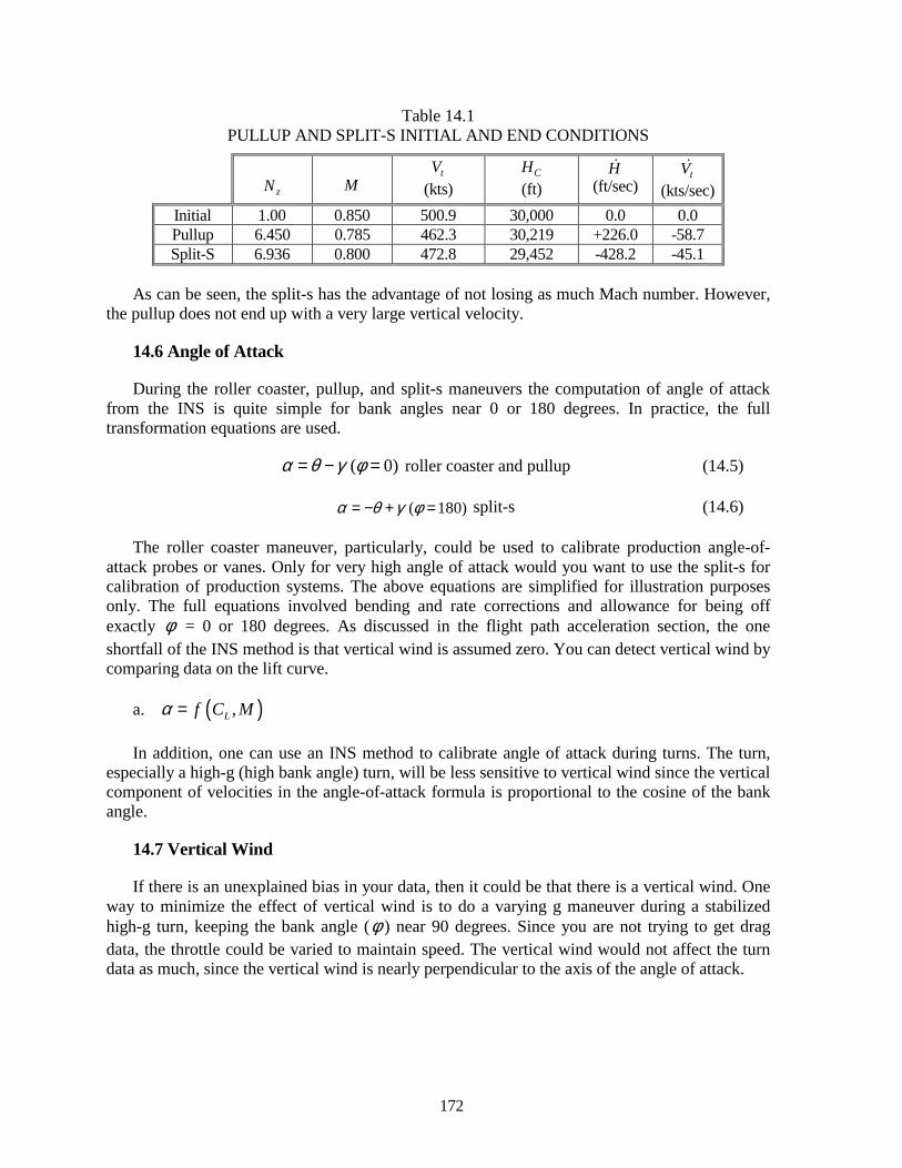
172

Table 14.1 PULLUP AND SPLIT-S INITIAL AND END CONDITIONS

zN

M

tV (kts)

CH (ft)

H! (ft/sec)

tV! (kts/sec)

Initial 1.00 0.850 500.9 30,000 0.0 0.0 Pullup 6.450 0.785 462.3 30,219 +226.0 -58.7 Split-S 6.936 0.800 472.8 29,452 -428.2 -45.1

As can be seen, the split-s has the advantage of not losing as much Mach number. However,

the pullup does not end up with a very large vertical velocity.

14.6 Angle of Attack

During the roller coaster, pullup, and split-s maneuvers the computation of angle of attack from the INS is quite simple for bank angles near 0 or 180 degrees. In practice, the full transformation equations are used.

( 0)α θ γ φ= − = roller coaster and pullup (14.5)

( 180)α θ γ φ= − + = split-s (14.6)

The roller coaster maneuver, particularly, could be used to calibrate production angle-of-attack probes or vanes. Only for very high angle of attack would you want to use the split-s for calibration of production systems. The above equations are simplified for illustration purposes only. The full equations involved bending and rate corrections and allowance for being off exactly φ = 0 or 180 degrees. As discussed in the flight path acceleration section, the one shortfall of the INS method is that vertical wind is assumed zero. You can detect vertical wind by comparing data on the lift curve.

a. ( ),Lf C Mα =

In addition, one can use an INS method to calibrate angle of attack during turns. The turn, especially a high-g (high bank angle) turn, will be less sensitive to vertical wind since the vertical component of velocities in the angle-of-attack formula is proportional to the cosine of the bank angle.

14.7 Vertical Wind

If there is an unexplained bias in your data, then it could be that there is a vertical wind. One way to minimize the effect of vertical wind is to do a varying g maneuver during a stabilized high-g turn, keeping the bank angle (φ ) near 90 degrees. Since you are not trying to get drag data, the throttle could be varied to maintain speed. The vertical wind would not affect the turn data as much, since the vertical wind is nearly perpendicular to the axis of the angle of attack.

173

15.0 SPECIAL PERFORMANCE TOPICS

15.1 Effect of Gravity on Performance

Below is the international gravity formula as adopted by the International Union of Geodesy and Geophysics as presented in Britannica Online.

2 40 978.03185 1 0.005278892 sin 0.000023462 sinγ ϕ ϕ = ⋅ + ⋅ + ⋅ cm/sec2 (15.1)

Where the symbology used by the International Union is as follows:

a. 0γ = sea level gravity (cm/sec2), and

b. ϕ = latitude (degrees).

In this text, we have used a rather simplified gravity model of g = constant = 32.174 ft/sec2. As of the writing of this text, that simplification is widely used in the conventional aircraft flight testing community. This topic will address the magnitude of error that this simplification produces. As will be seen, the error is quite small (<1 percent), but not zero.

First, we will take the liberty of changing the International Union’s sea level gravity symbology from 0γ to 0g .

Consider only a 1-g flight where the aircraft is unbanked and has zero vertical velocity and zero rate of change of vertical velocity. Under these conditions, the normal load factor ( zN ) would not be precisely 1.00. There are four variables: latitude, altitude, speed, and heading. We will consider them individually.

The internationally agreed upon exact conversion factor between meters (or metres in Great Britain) is 0.3048 (divide meters by 0.3048 to yield feet) and the number of centimeters (cm) in a meter is 100. Given that and using equation 15.1, some typical values of sea level gravity are shown in Table 15.1.

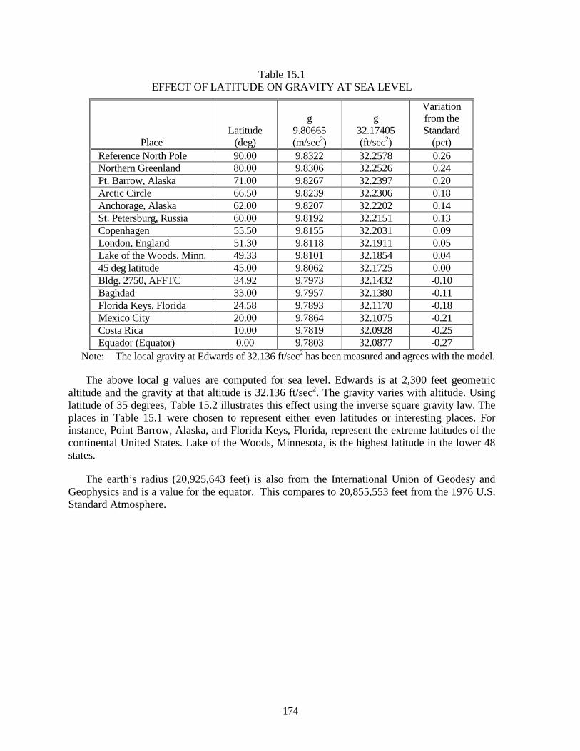
174

Table 15.1 EFFECT OF LATITUDE ON GRAVITY AT SEA LEVEL

Place

Latitude (deg)

g

9.80665 (m/sec2)

g

32.17405 (ft/sec2)

Variation from the Standard

(pct) Reference North Pole 90.00 9.8322 32.2578 0.26 Northern Greenland 80.00 9.8306 32.2526 0.24 Pt. Barrow, Alaska 71.00 9.8267 32.2397 0.20 Arctic Circle 66.50 9.8239 32.2306 0.18 Anchorage, Alaska 62.00 9.8207 32.2202 0.14 St. Petersburg, Russia 60.00 9.8192 32.2151 0.13 Copenhagen 55.50 9.8155 32.2031 0.09 London, England 51.30 9.8118 32.1911 0.05 Lake of the Woods, Minn. 49.33 9.8101 32.1854 0.04 45 deg latitude 45.00 9.8062 32.1725 0.00 Bldg. 2750, AFFTC 34.92 9.7973 32.1432 -0.10 Baghdad 33.00 9.7957 32.1380 -0.11 Florida Keys, Florida 24.58 9.7893 32.1170 -0.18 Mexico City 20.00 9.7864 32.1075 -0.21 Costa Rica 10.00 9.7819 32.0928 -0.25 Equador (Equator) 0.00 9.7803 32.0877 -0.27

Note: The local gravity at Edwards of 32.136 ft/sec2 has been measured and agrees with the model.

The above local g values are computed for sea level. Edwards is at 2,300 feet geometric altitude and the gravity at that altitude is 32.136 ft/sec2. The gravity varies with altitude. Using latitude of 35 degrees, Table 15.2 illustrates this effect using the inverse square gravity law. The places in Table 15.1 were chosen to represent either even latitudes or interesting places. For instance, Point Barrow, Alaska, and Florida Keys, Florida, represent the extreme latitudes of the continental United States. Lake of the Woods, Minnesota, is the highest latitude in the lower 48 states.

The earth’s radius (20,925,643 feet) is also from the International Union of Geodesy and Geophysics and is a value for the equator. This compares to 20,855,553 feet from the 1976 U.S. Standard Atmosphere.

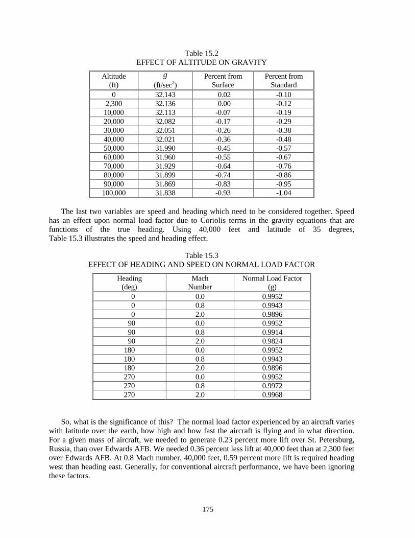
175

Table 15.2 EFFECT OF ALTITUDE ON GRAVITY

Altitude (ft)

g (ft/sec2)

Percent from Surface

Percent from Standard

0 32.143 0.02 -0.10 2,300 32.136 0.00 -0.12 10,000 32.113 -0.07 -0.19 20,000 32.082 -0.17 -0.29 30,000 32.051 -0.26 -0.38 40,000 32.021 -0.36 -0.48 50,000 31.990 -0.45 -0.57 60,000 31.960 -0.55 -0.67 70,000 31.929 -0.64 -0.76 80,000 31.899 -0.74 -0.86 90,000 31.869 -0.83 -0.95 100,000 31.838 -0.93 -1.04

The last two variables are speed and heading which need to be considered together. Speed

has an effect upon normal load factor due to Coriolis terms in the gravity equations that are functions of the true heading. Using 40,000 feet and latitude of 35 degrees, Table 15.3 illustrates the speed and heading effect.

Table 15.3 EFFECT OF HEADING AND SPEED ON NORMAL LOAD FACTOR

Heading (deg)

Mach Number

Normal Load Factor (g)

0 0.0 0.9952 0 0.8 0.9943 0 2.0 0.9896

90 0.0 0.9952 90 0.8 0.9914 90 2.0 0.9824

180 0.0 0.9952 180 0.8 0.9943 180 2.0 0.9896 270 0.0 0.9952 270 0.8 0.9972 270 2.0 0.9968

So, what is the significance of this? The normal load factor experienced by an aircraft varies with latitude over the earth, how high and how fast the aircraft is flying and in what direction. For a given mass of aircraft, we needed to generate 0.23 percent more lift over St. Petersburg, Russia, than over Edwards AFB. We needed 0.36 percent less lift at 40,000 feet than at 2,300 feet over Edwards AFB. At 0.8 Mach number, 40,000 feet, 0.59 percent more lift is required heading west than heading east. Generally, for conventional aircraft performance, we have been ignoring these factors.

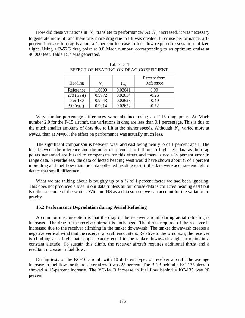
176

How did these variations in zN translate to performance? As zN increased, it was necessary to generate more lift and therefore, more drag due to lift was created. In cruise performance, a 1-percent increase in drag is about a 1-percent increase in fuel flow required to sustain stabilized flight. Using a B-52G drag polar at 0.8 Mach number, corresponding to an optimum cruise at 40,000 feet, Table 15.4 was generated.

Table 15.4 EFFECT OF HEADING ON DRAG COEFFICIENT

Heading

zN

DC

Percent from Reference

Reference 1.0000 0.02641 0.00 270 (west) 0.9972 0.02634 -0.26 0 or 180 0.9943 0.02628 -0.49 90 (east) 0.9914 0.02622 -0.72

Very similar percentage differences were obtained using an F-15 drag polar. At Mach

number 2.0 for the F-15 aircraft, the variations in drag are less than 0.1 percentage. This is due to the much smaller amounts of drag due to lift at the higher speeds. Although zN varied more at M=2.0 than at M=0.8, the effect on performance was actually much less.

The significant comparison is between west and east being nearly ½ of 1 percent apart. The bias between the reference and the other data tended to fall out in flight test data as the drag polars generated are biased to compensate for this effect and there is not a ½ percent error in range data. Nevertheless, the data collected heading west would have shown about ½ of 1 percent more drag and fuel flow than the data collected heading east, if the data were accurate enough to detect that small difference.

What we are talking about is roughly up to a ½ of 1-percent factor we had been ignoring. This does not produced a bias in our data (unless all our cruise data is collected heading east) but is rather a source of the scatter. With an INS as a data source, we can account for the variation in gravity.

15.2 Performance Degradation during Aerial Refueling

A common misconception is that the drag of the receiver aircraft during aerial refueling is increased. The drag of the receiver aircraft is unchanged. The thrust required of the receiver is increased due to the receiver climbing in the tanker downwash. The tanker downwash creates a negative vertical wind that the receiver aircraft encounters. Relative to the wind axis, the receiver is climbing at a flight path angle exactly equal to the tanker downwash angle to maintain a constant altitude. To sustain this climb, the receiver aircraft requires additional thrust and a resultant increase in fuel flow.

During tests of the KC-10 aircraft with 10 different types of receiver aircraft, the average increase in fuel flow for the receiver aircraft was 25 percent. The B-1B behind a KC-135 aircraft showed a 15-percent increase. The YC-141B increase in fuel flow behind a KC-135 was 20 percent.

177

To estimate the increase in thrust required for a receiver aircraft, you only need to know the theoretical downwash angle behind the tanker and then apply a downwash factor. The downwash factor (K) is simply a multiplicative factor to account for the fact that the receiver aircraft is in a flow field that is a combination of the tanker flow field and the free stream. For both the KE-3A and the B1-B aircraft, this K factor is about 0.5. The theoretical downwash angle ( 0ε ) is exactly twice the ideal angle of attack.

( )( )0

2 Lt

t

CAR

επ⋅

=⋅

(15.2)

where:

LtC = lift coefficient of the tanker aircraft, and

tAR = aspect ratio of the tanker aircraft.

The actual downwash angle is found (with a K of 0.5) to be approximately equal to the ideal angle of attack of the tanker.

( )Lt

tt

CAR

επ

=⋅

(15.3)

Then the increase in thrust of the receiver could be computed by the component of weight through the downwash angle. With respect to the wind axis, the receiver aircraft is climbing while behind a tanker in level flight.

sin( )n tF W ε∆ = ⋅ (15.4)

15.3 Performance Degradation during Terrain Following

Flight while performing terrain following results in an increase in average fuel flow when compared to flight at the same average Mach number and altitude level. While in the terrain following mode, the aircraft is constantly either pulling up or pushing over. In a pullup ( zN >1) the drag is increased over that for an zN =1 due to an increase in drag due to lift (or induced drag). In a pushover, ( zN <1) the drag is reduced due to a decrease in the drag due to lift. Because of the parabolic nature of the drag polar, the magnitude of the drag increase in the pullup is greater than the magnitude of the drag decrease in the pushover. The net effect is there is a net increase in average thrust required and a resultant increase in average fuel flow.

For the case of an aircraft with automatic terrain following and afterburner, the average increase in fuel flow can be substantial. Every time afterburner is used, the fuel flow increases dramatically. The thrust specific fuel consumption ( )tsfc will typically be less than 1.0 in non-afterburner and >2.0 in afterburner.

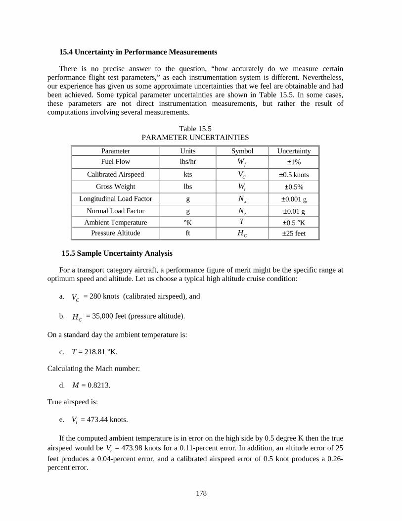
178

15.4 Uncertainty in Performance Measurements

There is no precise answer to the question, “how accurately do we measure certain performance flight test parameters,” as each instrumentation system is different. Nevertheless, our experience has given us some approximate uncertainties that we feel are obtainable and had been achieved. Some typical parameter uncertainties are shown in Table 15.5. In some cases, these parameters are not direct instrumentation measurements, but rather the result of computations involving several measurements.

Table 15.5 PARAMETER UNCERTAINTIES

Parameter Units Symbol Uncertainty Fuel Flow lbs/hr fW ±1%

Calibrated Airspeed kts CV ±0.5 knots Gross Weight lbs tW ±0.5%

Longitudinal Load Factor g xN ±0.001 g Normal Load Factor g zN ±0.01 g

Ambient Temperature °K T ±0.5 °K Pressure Altitude ft CH ±25 feet

15.5 Sample Uncertainty Analysis

For a transport category aircraft, a performance figure of merit might be the specific range at optimum speed and altitude. Let us choose a typical high altitude cruise condition:

a. CV = 280 knots (calibrated airspeed), and

b. CH = 35,000 feet (pressure altitude).

On a standard day the ambient temperature is:

c. T = 218.81 °K.

Calculating the Mach number:

d. M = 0.8213.

True airspeed is:

e. tV = 473.44 knots.

If the computed ambient temperature is in error on the high side by 0.5 degree K then the true airspeed would be tV = 473.98 knots for a 0.11-percent error. In addition, an altitude error of 25 feet produces a 0.04-percent error, and a calibrated airspeed error of 0.5 knot produces a 0.26-percent error.

179

At an / 10.0L D = , an error of 0.001 g in longitudinal load factor yields a 1.0-percent error in drag. We shall assume error in drag produces a 1.0-percent error in range factor. Then, for range factor ( RF ), we have the following errors:

a. tV 0.11 percent due to T error,

b. tV 0.04 percent due to CH error,

c. tV 0.26 percent due to CV error,

d. xN 1.00 percent,

e. tW 0.50 percent, and

f. fW 1.00 percent.

The root mean square (rms) of the three tV uncertainties computes to be 0.285 percent. The RMS of the four uncertainties computes to be 1.53 percent. Please note that carrying out the speeds to five significant figures did not imply that we could measure speeds to that level of accuracy. At the time of this handbook, with the advent of EGI even greater accuracies than those presented above may be achieved for airspeeds, altitudes, and flight path accelerations.

15.6 Wind Direction Definition

What may seem to be an improper definition of wind direction (from which the wind is blowing) may derive from ancient Greece. Improper in the sense that defining the wind direction as from which it is blowing is opposite from the vector direction of wind. In Britannica Online, a structure called the Tower of the Winds is discussed briefly. In about 100 BC an octagonal (eight-sided) marble structure, 42 feet high and 26 feet in diameter, was constructed. The eight sides face points of the compass (N, N-E, E, etc). It would seem logical that a wind blowing on the structure would be considered a positive wind. The wind would always be positive, since it would be blowing on some side of the structure – never away from the structure, so to speak. Therefore, if the wind were blowing directly on the north side of the Tower of the Winds, this positive wind would have a direction of north (0 degrees). This direction is the direction from which the wind is blowing, the same as the compass heading of the Tower. One could think of this Tower as either an aircraft control tower or an aircraft.

16.0 STANDARDIZATION

16.1 Introduction

For presentation and comparison purposes, performance data are usually corrected to standard conditions. The standard conditions are specified values of gross weight, pressure altitude, cg (center of gravity), and Mach number. Standard ambient temperature is usually based on the 1976 U.S. Standard Atmosphere. Standardization relies upon a predicted model of drag, thrust, and fuel flow. Usually, small corrections to standard day conditions are made, but these could be large when temperature is substantially off standard day. If there is a 10-percent error in the predicted model and we made 10-percent corrections to the data, we incurred only a 1- percent error in the standardized results. At the AFFTC in midsummer, the temperature at 30,000 feet is, on average, 10 degrees C hotter than standard day, which produces, typically, about a 10-percent decrease in thrust at MIL or MAX. The standardization is performed using an additive increment method.

16.2 Increment Method

The general principle of standardization is an additive increment method. The formulas used to standardize net thrust ( nF ), fuel flow ( fW ), and drag ( D ) are as follows:

( )ns nt ns ntF F F F′ ′= + − (16.1)

where:

nsF = standardized net thrust (pounds),

ntF = test day net thrust (pounds),

nsF ′ = standard day predicted net thrust (pounds), and

ntF ′ = test day predicted net thrust (pounds).

( )fs ft fs ftW W W W′ ′= + − (16.2)

where:

fsW = standardized fuel flow (pounds/hour),

ftW = test day fuel flow (pounds/hour),

fsW ′ = standard day predicted fuel flow (pounds/hour), and

ftW ′ = test day predicted fuel flow (pounds/hour).

Fuel flow is first standardized to a minimum fuel lower heating value (LHV), usually 18,400 Btu/pound.

18, 400

testft ft

LHVW W = ⋅

(16.3)

181

Typical test values of LHV are in the vicinity of 18,550 Btu/pound, which amounts to a ½-percent correction. The correction will generally increase fuel flow, since the spec is a minimum. That is, almost all actual fuel will have an LHV greater than the spec.

( )s t s tD D D D′ ′= + − (16.4)

where:

sD = standardized drag (pounds),

tD = test day drag (pounds),

sD ′ = predicted standard day drag (pounds), and

tD ′ = predicted test day drag (pounds).

t nt extD F F= − (16.5)

tex x tF N W= ⋅ = test day measured excess thrust (16.6)

Then,

( ) ( )s tex ex ns s nt tF F F D F D′ ′ ′ ′= + − − − (16.7)

The above equations illustrate the general principle. The test net thrust is determined, usually, from an in-flight thrust deck. The predicted thrust and fuel flows are determined from a prediction (or status) deck. These are described briefly in the thrust section. The predicted drags are obtained from a contractor-provided predicted drag model subroutine. The contractor drag model should include an accounting for skin friction drag. In lieu of that, formulas presented in the lift and drag section could be used.

Each maneuver involves a different parameter being adjusted to standard conditions but the basic method is the same incremental difference method. The standardization parameters for various maneuvers are discussed in the following text.

16.2.1 Climb/Descent

Excess thrust and fuel flow are standardized:

a. zN is computed.

16.2.2 Acceleration/Deceleration


a. zN = 1.0.

182

16.2.3 Accelerating/Decelerating Turn


a. zN is specified.

16.2.4 Cruise

Fuel flow is standardized:

a. zN = 1.0 (usually) (Note: a rare exception to the 1.0-g would be for standardizing data in an endurance turn.), and

b. Excess thrust = 0.0.

16.2.5 Thrust-Limited Turn

zN and fuel flow are standardized:

a. Excess thrust = 0.0.

16.3 Ratio Method

An alternative to the increment method of standardization is a method based upon ratios. The formulas for standard day net thrust, fuel flow, and drag would be as follows:

nsns nt

nt

FF FF

′ = ⋅

′ (16.8)

fsfs ft

ft

WW W

W

′ = ⋅

′

(16.9)

ss t

t

DD DD

′ = ⋅

′ (16.10)

Then, standard day excess thrust (sexF ) would be:

sex ns sF F D= − (16.11)

For fixed throttle maneuvers (climb, turn, and accel), the above equation would suffice. For cruise, where standard excess thrust should be zero, an iteration is required.

The question that needs to be answered is “what is the difference in the magnitude of difference between the ratio and difference methods?” Take the case of the standardized excess

183

thrust in acceleration. If there was zero error in both test day measured net thrust and in the thrust model, then there would be zero error in the standardization for both ratio and increment methods. From the above equations, let us write out the full

sexF formula for both increment and ratio methods.

s

ns sex nt t

nt t

F DF F DF D

′ ′ = ⋅ − ⋅

′ ′ ratio method (16.12)

However,

tt nt exD F F= − for both methods (16.13)

Then, the ratio method becomes:

s t

s ns sex ex nt nt

t nt t

D F DF F F FD F D

′ ′ ′ = ⋅ + ⋅ − ⋅

′ ′ ′ ratio method (16.14)

( ) ( )s tex ex ns nt s tF F F F D D′ ′ ′ ′= + − − − increment method (16.15)

Then, whichever method introduces the most error into the standardized excess thrust is a function of the errors in the prediction models. If the prediction models are in error by approximately a constant percentage, then the ratio method will introduce the least error. This is because the errors would cancel out when doing the division. Conversely, if the models are in error by approximately a constant magnitude, then the increment method will introduce the least error. This is due to the errors canceling out when doing the subtraction.

Either way, one is invariably introducing some errors (hopefully small) into your data by the very process of standardization. Standardization is performed as a means of convenient data presentation. One should recognize that a data point on a plot presented as standard conditions is a data point that was not flown. It represents an extrapolation of an actual test point. The following are two sources of error in standardization.

a. For cruise at high altitude, the standard day conditions may be unachievable. That is due to having sufficient thrust on a test day, but not on a standard day. The test day temperature may have been substantially colder than standard day giving the engine much more thrust than would be available on the warmer standard day. Your cruise standardization algorithm should check to assure that standard day drag is less than the maximum available thrust.

b. The engine may be in some manner limited (turbine temperature or rpm limit) on the test day. If this limiter is not accurately modeled in the status deck, then the correction to standard day will have errors. For instance, the engine may not be on this limit on the standard day, yielding additional thrust. Conversely, it may not be on the limit on the test day, but would be on the standard day.

184

17.0 A SAMPLE PERFORMANCE MODEL

17.1 Introduction

In this section, we will construct a performance model. The model will be highly idealized. The purpose of this section is to illustrate some general concepts. One should not assume that their drag, thrust, or fuel flow models would be the same as, or as simple as, those presented here.

17.2 Drag Model

17.2.1 Minimum Drag Coefficient

In order to illustrate the shape of performance parameters, such as specific excess power as a function of Mach number or altitude, we will construct a drag model. That drag model is fiction, but approximates that of an F-16 aircraft. Drag has three components. These are skin friction, profile drag, and drag due to lift. We could think of drag as having only two components: minimum drag and drag due to lift. Minimum drag is then the sum of profile drag and skin friction drag. Drag due to lift is also called induced drag. Profile drag is sometimes called form drag. For the purposes of our model, we will make up numbers for standard day at 30,000 feet pressure altitude. Then, our predicted skin friction drag formulas will be used to compute minimum drag at conditions other than standard day at 30,000 feet.

Our basic formula for drag coefficient is the AFFTC drag model formulation from the previous section. We will start by assuming that minDC = 0.0200 (200 drag counts) for Mach number < 0.80. That is a typical minimum drag coefficient for a wide range of aircraft. From the subsonic condition to Mach number = 1.0, the drag coefficient approximately doubles. Some data points were assumed and a curve fit was applied. Figure 17.1 is delta drag coefficient for the subsonic condition. The equation for minimum drag coefficient at any given Mach number is as follows:

min 0.0200D DC C= + ∆ (17.1)

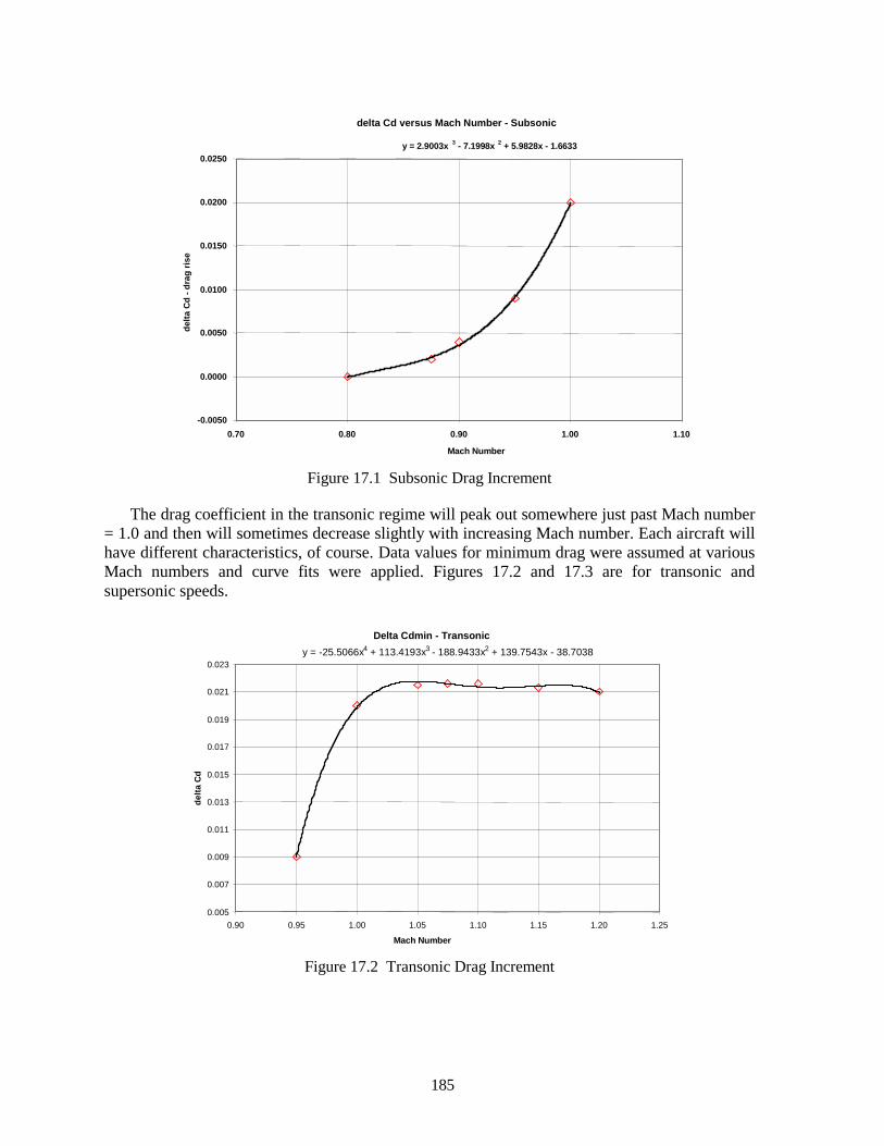
185

delta Cd versus Mach Number - Subsonic

y = 2.9003x 3 - 7.1998x 2 + 5.9828x - 1.6633

-0.0050

0.0000

0.0050

0.0100

0.0150

0.0200

0.0250

0.70 0.80 0.90 1.00 1.10

Mach Number

delta

Cd

- dra

g ris

e

Figure 17.1 Subsonic Drag Increment

The drag coefficient in the transonic regime will peak out somewhere just past Mach number = 1.0 and then will sometimes decrease slightly with increasing Mach number. Each aircraft will have different characteristics, of course. Data values for minimum drag were assumed at various Mach numbers and curve fits were applied. Figures 17.2 and 17.3 are for transonic and supersonic speeds.

Delta Cdmin - Transonicy = -25.5066x4 + 113.4193x3 - 188.9433x2 + 139.7543x - 38.7038

0.005

0.007

0.009

0.011

0.013

0.015

0.017

0.019

0.021

0.023

0.90 0.95 1.00 1.05 1.10 1.15 1.20 1.25

Mach Number

delta

Cd

Figure 17.2 Transonic Drag Increment

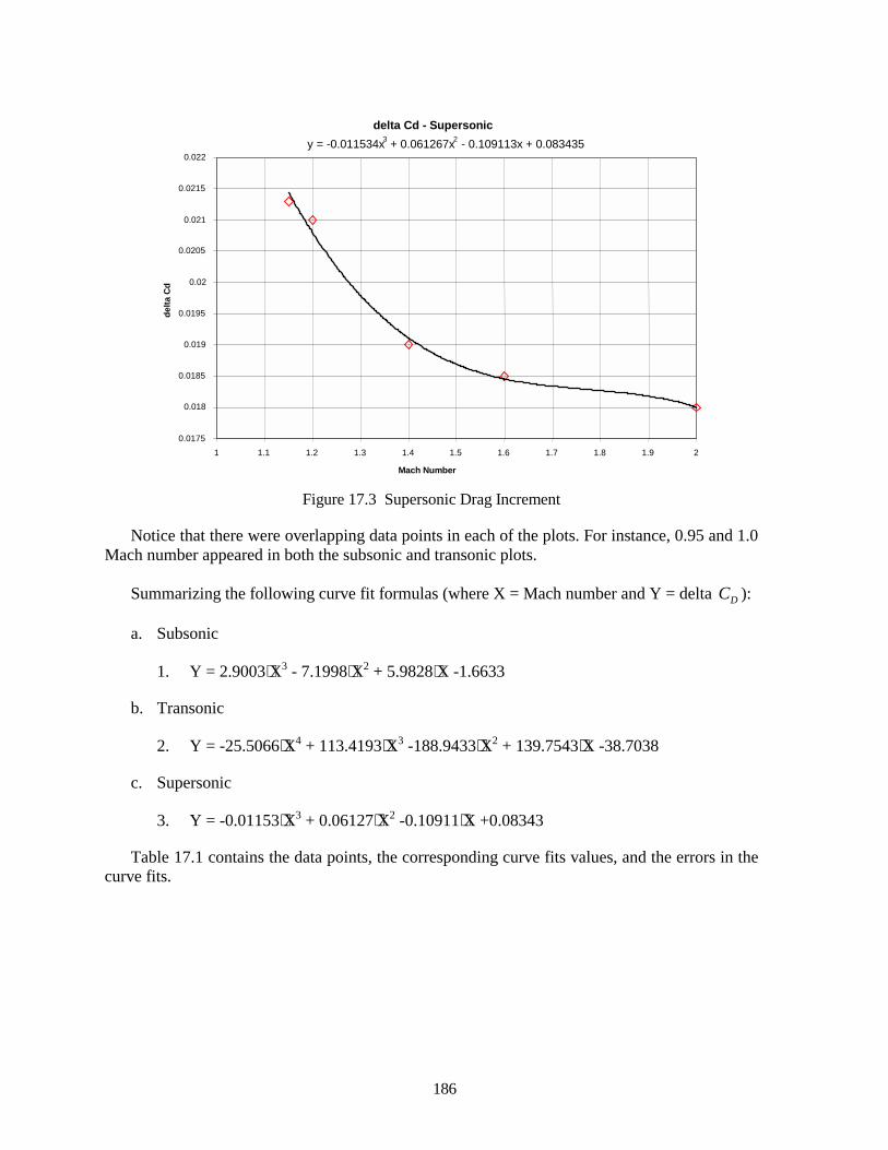
186

delta Cd - Supersonicy = -0.011534x3 + 0.061267x2 - 0.109113x + 0.083435

0.0175

0.018

0.0185

0.019

0.0195

0.02

0.0205

0.021

0.0215

0.022

1 1.1 1.2 1.3 1.4 1.5 1.6 1.7 1.8 1.9 2

Mach Number

delta

Cd

Figure 17.3 Supersonic Drag Increment

Notice that there were overlapping data points in each of the plots. For instance, 0.95 and 1.0 Mach number appeared in both the subsonic and transonic plots.

Summarizing the following curve fit formulas (where X = Mach number and Y = delta DC ):

a. Subsonic

1. Y = 2.9003⋅X3 - 7.1998⋅X2 + 5.9828⋅X -1.6633

b. Transonic

2. Y = -25.5066⋅X4 + 113.4193⋅X3 -188.9433⋅X2 + 139.7543⋅X -38.7038

c. Supersonic

3. Y = -0.01153⋅X3 + 0.06127⋅X2 -0.10911⋅X +0.08343

Table 17.1 contains the data points, the corresponding curve fits values, and the errors in the curve fits.

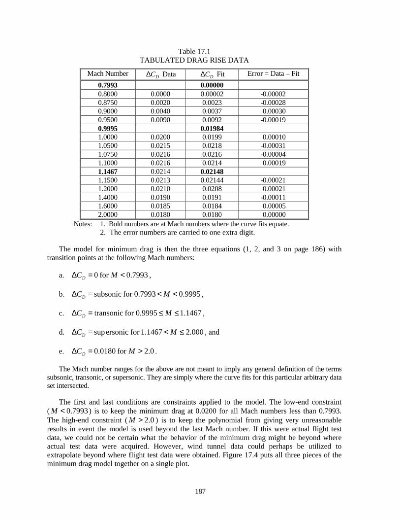
187

Table 17.1 TABULATED DRAG RISE DATA

Mach Number DC∆ Data DC∆ Fit Error = Data – Fit 0.7993 0.00000 0.8000 0.0000 0.00002 -0.00002 0.8750 0.0020 0.0023 -0.00028 0.9000 0.0040 0.0037 0.00030 0.9500 0.0090 0.0092 -0.00019 0.9995 0.01984 1.0000 0.0200 0.0199 0.00010 1.0500 0.0215 0.0218 -0.00031 1.0750 0.0216 0.0216 -0.00004 1.1000 0.0216 0.0214 0.00019 1.1467 0.0214 0.02148 1.1500 0.0213 0.02144 -0.00021 1.2000 0.0210 0.0208 0.00021 1.4000 0.0190 0.0191 -0.00011 1.6000 0.0185 0.0184 0.00005 2.0000 0.0180 0.0180 0.00000

Notes: 1. Bold numbers are at Mach numbers where the curve fits equate. 2. The error numbers are carried to one extra digit.

The model for minimum drag is then the three equations (1, 2, and 3 on page 186) with transition points at the following Mach numbers:

a. 0 for 0.7993DC M∆ = < ,

b. subsonic for 0.7993 0.9995DC M∆ = < < ,

c. transonic for 0.9995 1.1467DC M∆ = ≤ ≤ ,

d. supersonic for 1.1467 2.000DC M∆ = < ≤ , and

e. 0.0180 for 2.0DC M∆ = > .

The Mach number ranges for the above are not meant to imply any general definition of the terms subsonic, transonic, or supersonic. They are simply where the curve fits for this particular arbitrary data set intersected.

The first and last conditions are constraints applied to the model. The low-end constraint ( 0.7993M < ) is to keep the minimum drag at 0.0200 for all Mach numbers less than 0.7993. The high-end constraint ( 2.0M > ) is to keep the polynomial from giving very unreasonable results in event the model is used beyond the last Mach number. If this were actual flight test data, we could not be certain what the behavior of the minimum drag might be beyond where actual test data were acquired. However, wind tunnel data could perhaps be utilized to extrapolate beyond where flight test data were obtained. Figure 17.4 puts all three pieces of the minimum drag model together on a single plot.

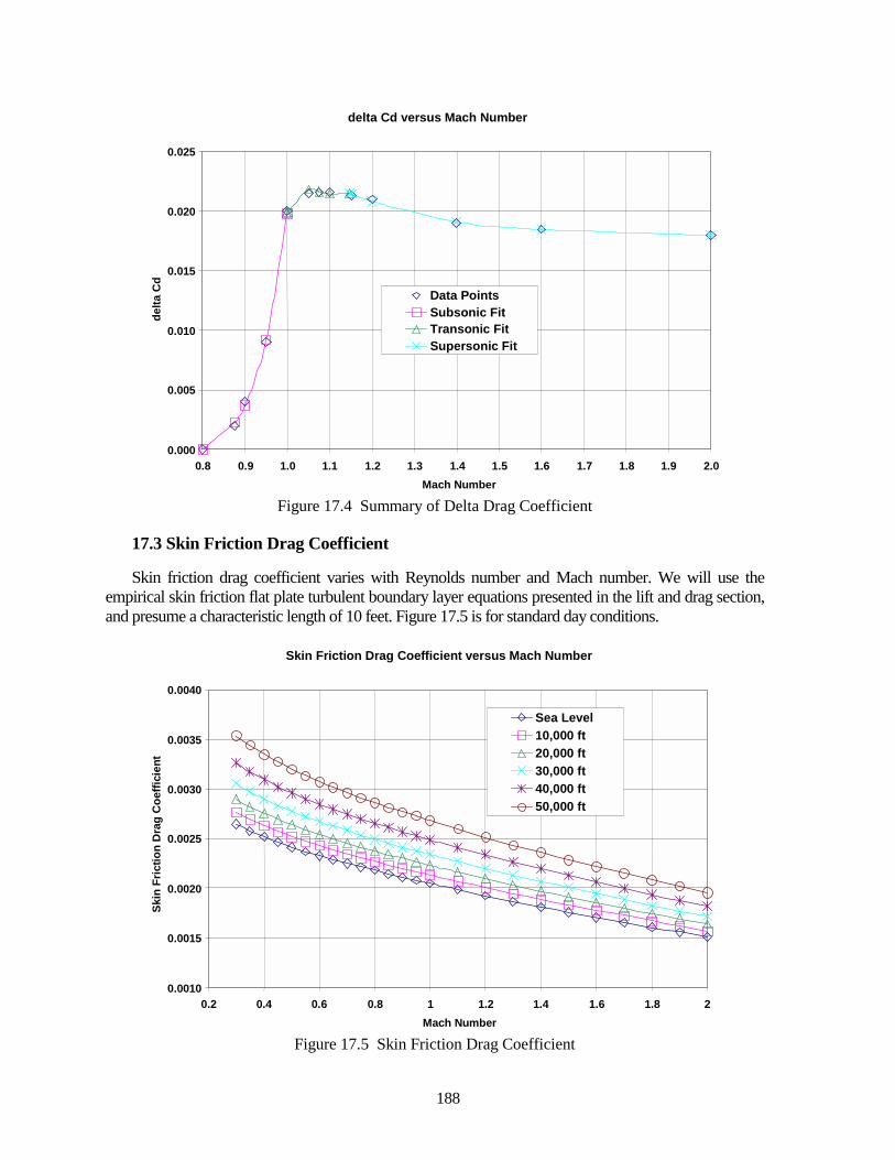
188

delta Cd versus Mach Number

0.000

0.005

0.010

0.015

0.020

0.025

0.8 0.9 1.0 1.1 1.2 1.3 1.4 1.5 1.6 1.7 1.8 1.9 2.0Mach Number

delta

Cd

Data PointsSubsonic FitTransonic FitSupersonic Fit

Figure 17.4 Summary of Delta Drag Coefficient

17.3 Skin Friction Drag Coefficient

Skin friction drag coefficient varies with Reynolds number and Mach number. We will use the empirical skin friction flat plate turbulent boundary layer equations presented in the lift and drag section, and presume a characteristic length of 10 feet. Figure 17.5 is for standard day conditions.

Skin Friction Drag Coefficient versus Mach Number

0.0010

0.0015

0.0020

0.0025

0.0030

0.0035

0.0040

0.2 0.4 0.6 0.8 1 1.2 1.4 1.6 1.8 2Mach Number

Skin

Fric

tion

Dra

g C

oeffi

cien

t

Sea Level10,000 ft20,000 ft30,000 ft40,000 ft50,000 ft

Figure 17.5 Skin Friction Drag Coefficient

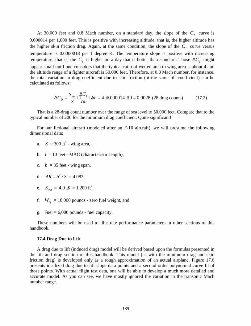
189

At 30,000 feet and 0.8 Mach number, on a standard day, the slope of the fC curve is 0.000014 per 1,000 feet. This is positive with increasing altitude; that is, the higher altitude has the higher skin friction drag. Again, at the same condition, the slope of the fC curve versus temperature is 0.0000018 per 1 degree K. The temperature slope is positive with increasing temperature; that is, the fC is higher on a day that is hotter than standard. Those fC∆ might appear small until one considers that the typical ratio of wetted area to wing area is about 4 and the altitude range of a fighter aircraft is 50,000 feet. Therefore, at 0.8 Mach number, for instance, the total variation in drag coefficient due to skin friction (at the same lift coefficient) can be calculated as follows:

4 0.000014 50 0.0028fwetD

CSC hS h

∆∆ = ⋅ ⋅∆ = ⋅ ⋅ =

∆ (28 drag counts) (17.2)

That is a 28-drag count number over the range of sea level to 50,000 feet. Compare that to the typical number of 200 for the minimum drag coefficient. Quite significant!

For our fictional aircraft (modeled after an F-16 aircraft), we will presume the following dimensional data:

a. S = 300 ft2 - wing area,

b. l = 10 feet - MAC (characteristic length),

c. b = 35 feet - wing span,

d. 2 /AR b S= = 4.083,

e. wetS = 4.0 S⋅ = 1,200 ft2,

f. ZfW = 18,000 pounds - zero fuel weight, and

g. Fuel = 6,000 pounds - fuel capacity.

These numbers will be used to illustrate performance parameters in other sections of this handbook.

17.4 Drag Due to Lift

A drag due to lift (induced drag) model will be derived based upon the formulas presented in the lift and drag section of this handbook. This model (as with the minimum drag and skin friction drag) is developed only as a rough approximation of an actual airplane. Figure 17.6 presents idealized drag due to lift slope data points and a second-order polynomial curve fit of those points. With actual flight test data, one will be able to develop a much more detailed and accurate model. As you can see, we have mostly ignored the variation in the transonic Mach number range.

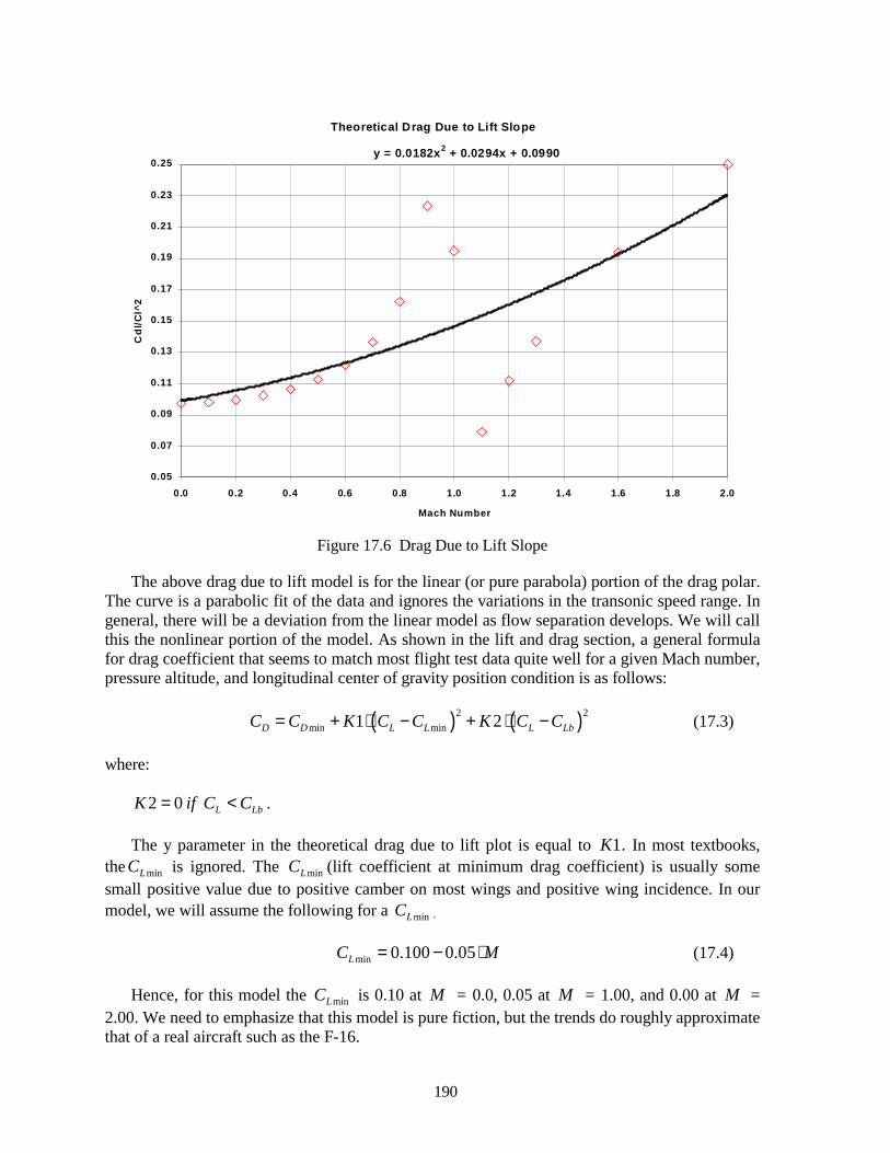
190

Theoretical Drag Due to Lift Slope

y = 0.0182x2 + 0.0294x + 0.0990

0.05

0.07

0.09

0.11

0.13

0.15

0.17

0.19

0.21

0.23

0.25

0.0 0.2 0.4 0.6 0.8 1.0 1.2 1.4 1.6 1.8 2.0

Mach Number

Cdl

/Cl^

2

Figure 17.6 Drag Due to Lift Slope

The above drag due to lift model is for the linear (or pure parabola) portion of the drag polar. The curve is a parabolic fit of the data and ignores the variations in the transonic speed range. In general, there will be a deviation from the linear model as flow separation develops. We will call this the nonlinear portion of the model. As shown in the lift and drag section, a general formula for drag coefficient that seems to match most flight test data quite well for a given Mach number, pressure altitude, and longitudinal center of gravity position condition is as follows:

( ) ( )2 2min min1 2D D L L L LbC C K C C K C C= + ⋅ − + ⋅ − (17.3)

where:

2 0 L LbK if C C= < .

The y parameter in the theoretical drag due to lift plot is equal to 1K . In most textbooks, the minLC is ignored. The minLC (lift coefficient at minimum drag coefficient) is usually some small positive value due to positive camber on most wings and positive wing incidence. In our model, we will assume the following for a minLC .

min 0.100 0.05LC M= − ⋅ (17.4)

Hence, for this model the minLC is 0.10 at M = 0.0, 0.05 at M = 1.00, and 0.00 at M = 2.00. We need to emphasize that this model is pure fiction, but the trends do roughly approximate that of a real aircraft such as the F-16.

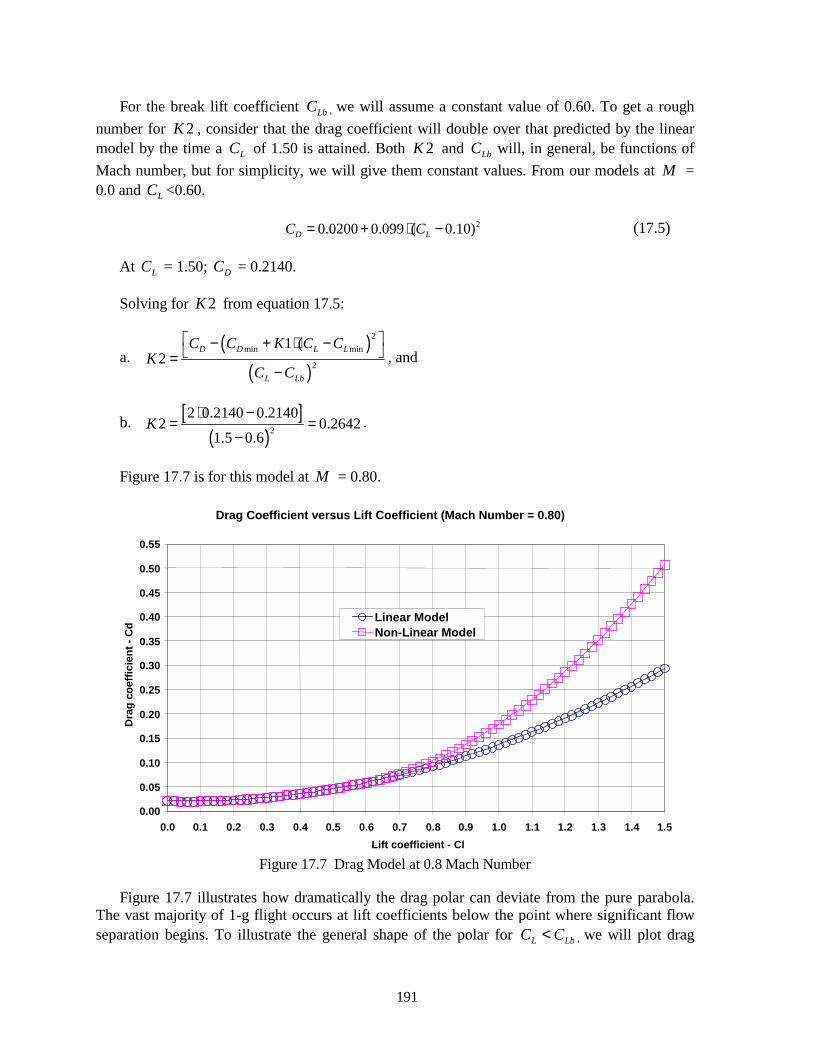
191

For the break lift coefficient LbC , we will assume a constant value of 0.60. To get a rough number for 2K , consider that the drag coefficient will double over that predicted by the linear model by the time a LC of 1.50 is attained. Both 2K and LbC will, in general, be functions of Mach number, but for simplicity, we will give them constant values. From our models at M = 0.0 and LC <0.60.

20.0200 0.099 ( 0.10)D LC C= + ⋅ − (17.5)

At LC = 1.50; DC = 0.2140.

Solving for 2K from equation 17.5:

a. ( )

( )

2min min

2

1 (2

D D L L

L Lb

C C K C CK

C C

− + ⋅ − =−

, and

b. [ ]( )2

2 0.2140 0.21402 0.2642

1.5 0.6K

⋅ −= =

−.

Figure 17.7 is for this model at M = 0.80.

Drag Coefficient versus Lift Coefficient (Mach Number = 0.80)

0.00

0.05

0.10

0.15

0.20

0.25

0.30

0.35

0.40

0.45

0.50

0.55

0.0 0.1 0.2 0.3 0.4 0.5 0.6 0.7 0.8 0.9 1.0 1.1 1.2 1.3 1.4 1.5Lift coefficient - Cl

Dra

g co

effic

ient

- C

d

Linear ModelNon-Linear Model

Figure 17.7 Drag Model at 0.8 Mach Number

Figure 17.7 illustrates how dramatically the drag polar can deviate from the pure parabola. The vast majority of 1-g flight occurs at lift coefficients below the point where significant flow separation begins. To illustrate the general shape of the polar for L LbC C< , we will plot drag

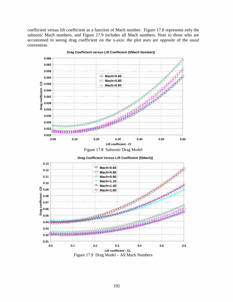
192

coefficient versus lift coefficient as a function of Mach number. Figure 17.8 represents only the subsonic Mach numbers, and Figure 17.9 includes all Mach numbers. Note to those who are accustomed to seeing drag coefficient on the x-axis: the plot axes are opposite of the usual convention.

Drag Coefficient versus Lift Coefficient {f(Mach Number)}

0.018

0.022

0.026

0.030

0.034

0.038

0.042

0.046

0.050

0.054

0.058

0.062

0.066

0.00 0.10 0.20 0.30 0.40 0.50 0.60Lift coefficient - Cl

Dra

g co

effic

ient

- C

d

Mach=0.60Mach=0.80Mach=0.90

Figure 17.8 Subsonic Drag Model

Drag Coefficient Versus Lift Coefficient {f(Mach)}

0.01

0.02

0.03

0.04

0.05

0.06

0.07

0.08

0.09

0.10

0.11

0.12

0.13

0.0 0.1 0.2 0.3 0.4 0.5 0.6Lift coefficient - CL

Dra

g co

effic

ient

- C

D

Mach=0.60Mach=0.80Mach=0.90Mach=1.10Mach=1.40Mach=1.60

Figure 17.9 Drag Model – All Mach Numbers

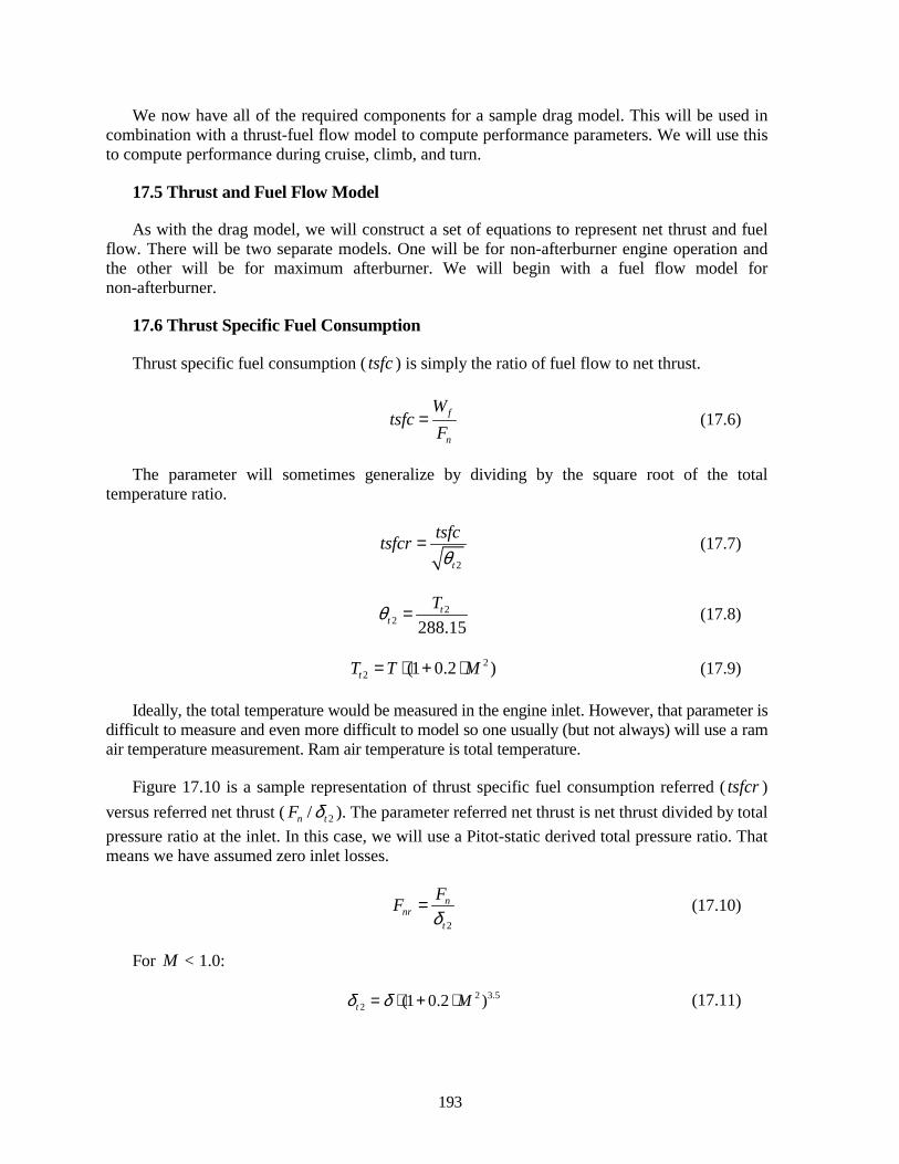
193

We now have all of the required components for a sample drag model. This will be used in combination with a thrust-fuel flow model to compute performance parameters. We will use this to compute performance during cruise, climb, and turn.

17.5 Thrust and Fuel Flow Model

As with the drag model, we will construct a set of equations to represent net thrust and fuel flow. There will be two separate models. One will be for non-afterburner engine operation and the other will be for maximum afterburner. We will begin with a fuel flow model for non-afterburner.

17.6 Thrust Specific Fuel Consumption

Thrust specific fuel consumption ( tsfc ) is simply the ratio of fuel flow to net thrust.

f

n

Wtsfc

F= (17.6)

The parameter will sometimes generalize by dividing by the square root of the total temperature ratio.

2t

tsfctsfcrθ

= (17.7)

22 288.15

tt

Tθ = (17.8)

22 (1 0.2 )tT T M= ⋅ + ⋅ (17.9)

Ideally, the total temperature would be measured in the engine inlet. However, that parameter is difficult to measure and even more difficult to model so one usually (but not always) will use a ram air temperature measurement. Ram air temperature is total temperature.

Figure 17.10 is a sample representation of thrust specific fuel consumption referred ( tsfcr ) versus referred net thrust ( 2/n tF δ ). The parameter referred net thrust is net thrust divided by total pressure ratio at the inlet. In this case, we will use a Pitot-static derived total pressure ratio. That means we have assumed zero inlet losses.

2

nnr

t

FFδ

= (17.10)

For M < 1.0:

2 3.52 (1 0.2 )t Mδ δ= ⋅ + ⋅ (17.11)

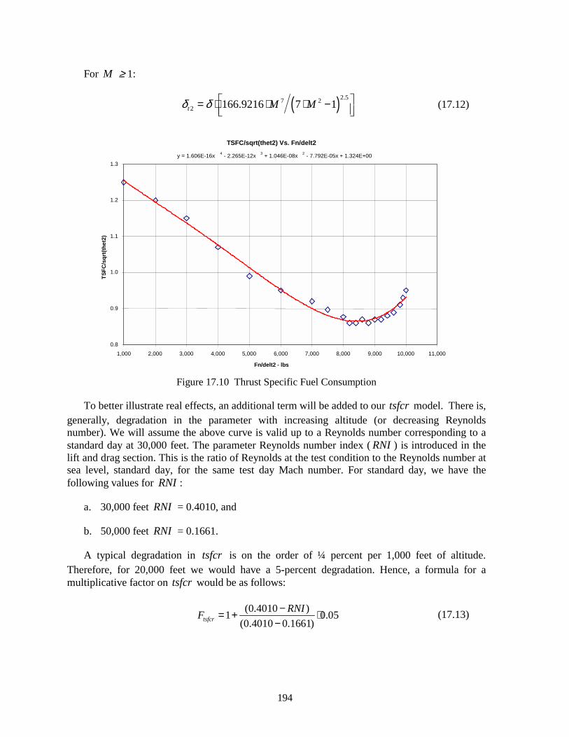
194

For M ≥ 1:

( )2.57 22 166.9216 7 1t M Mδ δ = ⋅ ⋅ ⋅ −

(17.12)

TSFC/sqrt(thet2) Vs. Fn/delt2

y = 1.606E-16x 4 - 2.265E-12x 3 + 1.046E-08x 2 - 7.792E-05x + 1.324E+00

0.8

0.9

1.0

1.1

1.2

1.3

1,000 2,000 3,000 4,000 5,000 6,000 7,000 8,000 9,000 10,000 11,000

Fn/delt2 - lbs

TSFC

/sqr

t(the

t2)

Figure 17.10 Thrust Specific Fuel Consumption

To better illustrate real effects, an additional term will be added to our tsfcr model. There is, generally, degradation in the parameter with increasing altitude (or decreasing Reynolds number). We will assume the above curve is valid up to a Reynolds number corresponding to a standard day at 30,000 feet. The parameter Reynolds number index ( RNI ) is introduced in the lift and drag section. This is the ratio of Reynolds at the test condition to the Reynolds number at sea level, standard day, for the same test day Mach number. For standard day, we have the following values for RNI :

a. 30,000 feet RNI = 0.4010, and

b. 50,000 feet RNI = 0.1661.

A typical degradation in tsfcr is on the order of ¼ percent per 1,000 feet of altitude. Therefore, for 20,000 feet we would have a 5-percent degradation. Hence, a formula for a multiplicative factor on tsfcr would be as follows:

(0.4010 )1 0.05(0.4010 0.1661)tsfcr

RNIF −= + ⋅−

(17.13)

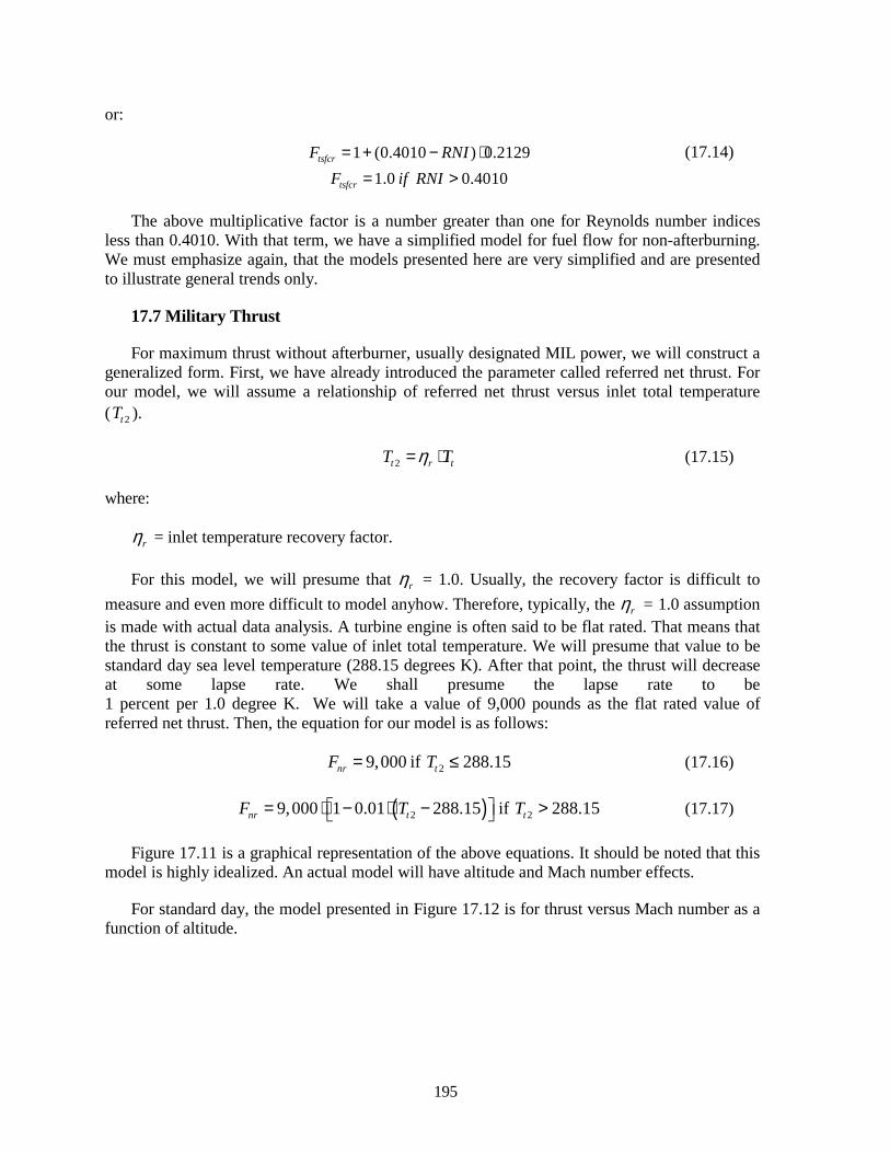
195

or:

1 (0.4010 ) 0.2129tsfcrF RNI= + − ⋅ (17.14) 1.0 0.4010tsfcrF if RNI= >

The above multiplicative factor is a number greater than one for Reynolds number indices less than 0.4010. With that term, we have a simplified model for fuel flow for non-afterburning. We must emphasize again, that the models presented here are very simplified and are presented to illustrate general trends only.

17.7 Military Thrust

For maximum thrust without afterburner, usually designated MIL power, we will construct a generalized form. First, we have already introduced the parameter called referred net thrust. For our model, we will assume a relationship of referred net thrust versus inlet total temperature ( 2tT ).

2t r tT Tη= ⋅ (17.15)

where:

rη = inlet temperature recovery factor.

For this model, we will presume that rη = 1.0. Usually, the recovery factor is difficult to measure and even more difficult to model anyhow. Therefore, typically, the rη = 1.0 assumption is made with actual data analysis. A turbine engine is often said to be flat rated. That means that the thrust is constant to some value of inlet total temperature. We will presume that value to be standard day sea level temperature (288.15 degrees K). After that point, the thrust will decrease at some lapse rate. We shall presume the lapse rate to be 1 percent per 1.0 degree K. We will take a value of 9,000 pounds as the flat rated value of referred net thrust. Then, the equation for our model is as follows:

29,000 if 288.15nr tF T= ≤ (17.16)

( )2 29,000 1 0.01 288.15 if 288.15nr t tF T T = ⋅ − ⋅ − > (17.17)

Figure 17.11 is a graphical representation of the above equations. It should be noted that this model is highly idealized. An actual model will have altitude and Mach number effects.

For standard day, the model presented in Figure 17.12 is for thrust versus Mach number as a function of altitude.

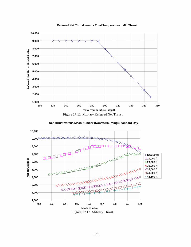
196

Referred Net Thrust versus Total Temperature: MIL Thrust

1,000

2,000

3,000

4,000

5,000

6,000

7,000

8,000

9,000

10,000

200 220 240 260 280 300 320 340 360 380Total Temperature - deg K

Ref

erre

d N

et T

hrus

t Fn/

delt2

- lb

s

Figure 17.11 Military Referred Net Thrust

Net Thrust versus Mach Number (Nonafterburning) Standard Day

1,000

2,000

3,000

4,000

5,000

6,000

7,000

8,000

9,000

10,000

0.2 0.3 0.4 0.5 0.6 0.7 0.8 0.9 1.0Mach Number

Net

Thr

ust (

lbs)

Sea Level10,000 ft20,000 ft30,000 ft35,000 ft40,000 ft42,500 ft

Figure 17.12 Military Thrust

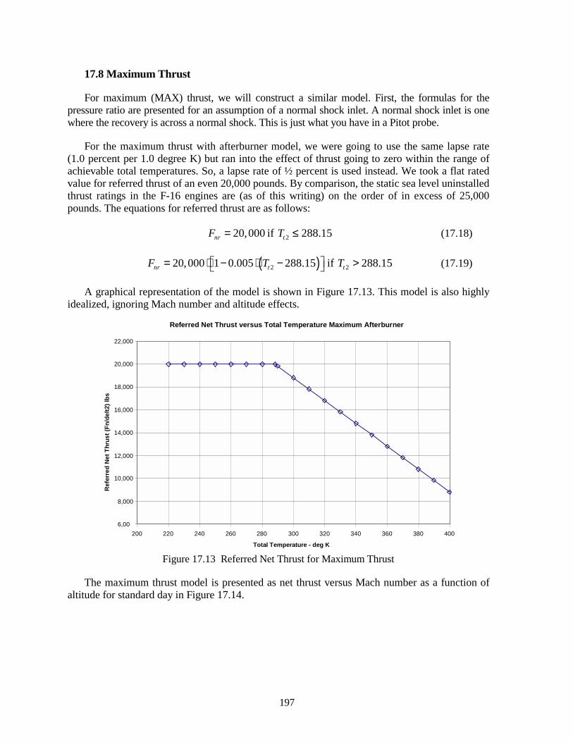
197

17.8 Maximum Thrust

For maximum (MAX) thrust, we will construct a similar model. First, the formulas for the pressure ratio are presented for an assumption of a normal shock inlet. A normal shock inlet is one where the recovery is across a normal shock. This is just what you have in a Pitot probe.

For the maximum thrust with afterburner model, we were going to use the same lapse rate (1.0 percent per 1.0 degree K) but ran into the effect of thrust going to zero within the range of achievable total temperatures. So, a lapse rate of ½ percent is used instead. We took a flat rated value for referred thrust of an even 20,000 pounds. By comparison, the static sea level uninstalled thrust ratings in the F-16 engines are (as of this writing) on the order of in excess of 25,000 pounds. The equations for referred thrust are as follows:

220,000 if 288.15nr tF T= ≤ (17.18)

( )2 220,000 1 0.005 288.15 if 288.15nr t tF T T = ⋅ − ⋅ − > (17.19)

A graphical representation of the model is shown in Figure 17.13. This model is also highly idealized, ignoring Mach number and altitude effects.

Referred Net Thrust versus Total Temperature Maximum Afterburner

6,00

8,000

10,000

12,000

14,000

16,000

18,000

20,000

22,000

200 220 240 260 280 300 320 340 360 380 400

Total Temperature - deg K

Ref

erre

d N

et T

hrus

t (Fn

/del

t2) l

bs

Figure 17.13 Referred Net Thrust for Maximum Thrust

The maximum thrust model is presented as net thrust versus Mach number as a function of altitude for standard day in Figure 17.14.

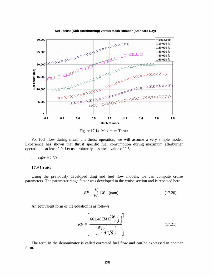
198

Net Thrust (with Afterburning) versus Mach Number (Standard Day)

0

5,000

10,000

15,000

20,000

25,000

30,000

0.2 0.4 0.6 0.8 1.0 1.2 1.4 1.6 1.8Mach Number

Net

Thr

ust (

lbs)


Figure 17.14 Maximum Thrust

For fuel flow during maximum thrust operation, we will assume a very simple model. Experience has shown that thrust specific fuel consumption during maximum afterburner operation is at least 2.0. Let us, arbitrarily, assume a value of 2.5:

a. 2.50tsfcr = .

17.9 Cruise

Using the previously developed drag and fuel flow models, we can compute cruise parameters. The parameter range factor was developed in the cruise section and is repeated here.

tt

f

VRF WW

= ⋅ (nam) (17.20)

An equivalent form of the equation is as follows:

661.48 t

f

WMRF

Wδ

δ θ

⋅ ⋅ = ⋅

(17.21)

The term in the denominator is called corrected fuel flow and can be expressed in another form.

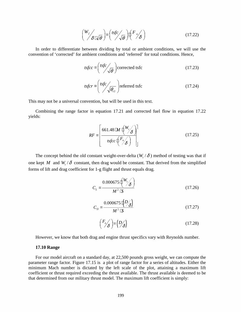
199

f nW Ftsfcδδ θ θ

= ⋅ ⋅ (17.22)

In order to differentiate between dividing by total or ambient conditions, we will use the convention of ‘corrected’ for ambient conditions and ‘referred’ for total conditions. Hence,

corrected tsfctsfctsfccθ

=

(17.23)

2

referred tsfct

tsfctsfcrθ

=

(17.24)

This may not be a universal convention, but will be used in this text.

Combining the range factor in equation 17.21 and corrected fuel flow in equation 17.22 yields:

661.48 t

n

WMRF

Ftsfcc

δ

δ

⋅ ⋅ = ⋅

(17.25)

The concept behind the old constant weight-over-delta ( /tW δ ) method of testing was that if one kept M and /tW δ constant, then drag would be constant. That derived from the simplified forms of lift and drag coefficient for 1-g flight and thrust equals drag.

2

0.000675 t

L

W

CM S

δ ⋅ =⋅

(17.26)

( )

2

0.000675D

DC

M Sδ⋅

=⋅

(17.27)

( )nF Dδ δ

=

(17.28)

However, we know that both drag and engine thrust specifics vary with Reynolds number.

17.10 Range

For our model aircraft on a standard day, at 22,500 pounds gross weight, we can compute the parameter range factor. Figure 17.15 is a plot of range factor for a series of altitudes. Either the minimum Mach number is dictated by the left scale of the plot, attaining a maximum lift coefficient or thrust required exceeding the thrust available. The thrust available is deemed to be that determined from our military thrust model. The maximum lift coefficient is simply:

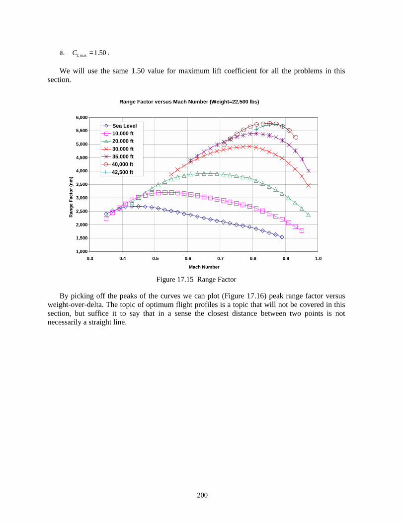
200

a. max 1.50LC = .

We will use the same 1.50 value for maximum lift coefficient for all the problems in this section.

Range Factor versus Mach Number (Weight=22,500 lbs)

1,000

1,500

2,000

2,500

3,000

3,500

4,000

4,500

5,000

5,500

6,000

0.3 0.4 0.5 0.6 0.7 0.8 0.9 1.0

Mach Number

Ran

ge F

acto

r (nm

)


Figure 17.15 Range Factor

By picking off the peaks of the curves we can plot (Figure 17.16) peak range factor versus weight-over-delta. The topic of optimum flight profiles is a topic that will not be covered in this section, but suffice it to say that in a sense the closest distance between two points is not necessarily a straight line.

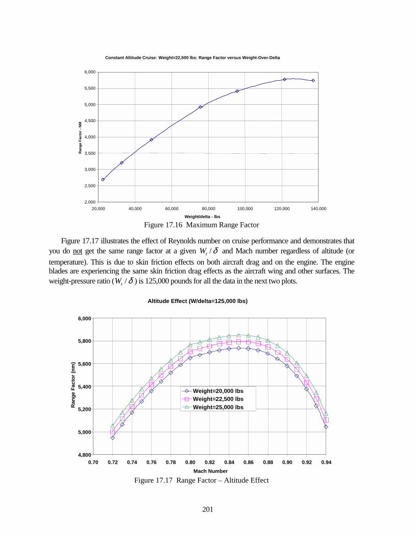
201

Constant Altitude Cruise: Weight=22,500 lbs: Range Factor versus Weight-Over-Delta

2,000

2,500

3,000

3,500

4,000

4,500

5,000

5,500

6,000

20,000 40,000 60,000 80,000 100,000 120,000 140,000

Weight/delta - lbs

Ran

ge F

acto

r - N

M

Figure 17.16 Maximum Range Factor

Figure 17.17 illustrates the effect of Reynolds number on cruise performance and demonstrates that you do not get the same range factor at a given /tW δ and Mach number regardless of altitude (or temperature). This is due to skin friction effects on both aircraft drag and on the engine. The engine blades are experiencing the same skin friction drag effects as the aircraft wing and other surfaces. The weight-pressure ratio ( /tW δ ) is 125,000 pounds for all the data in the next two plots.

Altitude Effect (W/delta=125,000 lbs)

4,800

5,000

5,200

5,400

5,600

5,800

6,000

0.70 0.72 0.74 0.76 0.78 0.80 0.82 0.84 0.86 0.88 0.90 0.92 0.94Mach Number

Ran

ge F

acto

r (nm

)

Weight=20,000 lbsWeight=22,500 lbsWeight=25,000 lbs

Figure 17.17 Range Factor – Altitude Effect

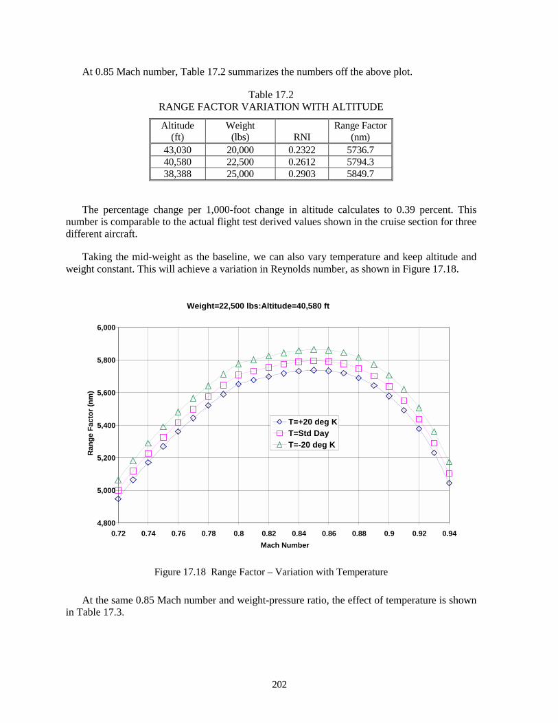
202

At 0.85 Mach number, Table 17.2 summarizes the numbers off the above plot.

Table 17.2 RANGE FACTOR VARIATION WITH ALTITUDE

Altitude (ft)

Weight (lbs)

RNI

Range Factor (nm)

43,030 20,000 0.2322 5736.7 40,580 22,500 0.2612 5794.3 38,388 25,000 0.2903 5849.7

The percentage change per 1,000-foot change in altitude calculates to 0.39 percent. This number is comparable to the actual flight test derived values shown in the cruise section for three different aircraft.

Taking the mid-weight as the baseline, we can also vary temperature and keep altitude and weight constant. This will achieve a variation in Reynolds number, as shown in Figure 17.18.

Weight=22,500 lbs:Altitude=40,580 ft

4,800

5,000

5,200

5,400

5,600

5,800

6,000

0.72 0.74 0.76 0.78 0.8 0.82 0.84 0.86 0.88 0.9 0.92 0.94Mach Number

Ran

ge F

acto

r (nm

)

T=+20 deg KT=Std DayT=-20 deg K

Figure 17.18 Range Factor – Variation with Temperature

At the same 0.85 Mach number and weight-pressure ratio, the effect of temperature is shown in Table 17.3.

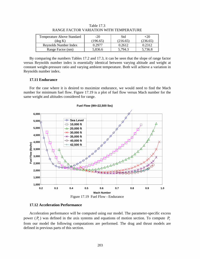
203

Table 17.3 RANGE FACTOR VARIATION WITH TEMPERATURE

Temperature Above Standard (deg K)

-20 (196.65)

Std (216.65)

+20 (236.65)

Reynolds Number Index 0.2977 0.2612 0.2312 Range Factor (nm) 5,836.6 5,794.3 5,736.8

By comparing the numbers Tables 17.2 and 17.3, it can be seen that the slope of range factor

versus Reynolds number index is essentially identical between varying altitude and weight at constant weight-pressure ratio and varying ambient temperature. Both will achieve a variation in Reynolds number index.

17.11 Endurance

For the case where it is desired to maximize endurance, we would need to find the Mach number for minimum fuel flow. Figure 17.19 is a plot of fuel flow versus Mach number for the same weight and altitudes considered for range.

Fuel Flow (Wt=22,500 lbs)

1,000

1,500

2,000

2,500

3,000

3,500

4,000

4,500

5,000

5,500

6,000

0.2 0.3 0.4 0.5 0.6 0.7 0.8 0.9 1.0Mach Number

Fuel

Flo

w (l

bs/h

r)


Figure 17.19 Fuel Flow - Endurance

17.12 Acceleration Performance

Acceleration performance will be computed using our model. The parameter-specific excess power ( sP ) was defined in the axis systems and equations of motion section. To compute sP from our model the following computations are performed. The drag and thrust models are defined in previous parts of this section.

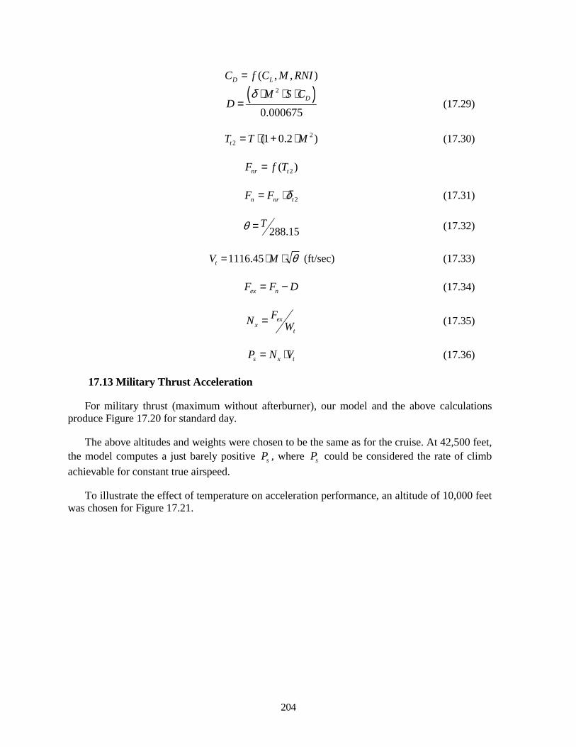
204

( , , )D LC f C M RNI=

( )2

0.000675DM S C

Dδ ⋅ ⋅ ⋅

= (17.29)

22 (1 0.2 )tT T M= ⋅ + ⋅ (17.30)

2( )nr tF f T=

2n nr tF F δ= ⋅ (17.31)

288.15Tθ = (17.32)

1116.45tV M θ= ⋅ ⋅ (ft/sec) (17.33)

ex nF F D= − (17.34)

exx

t

FN W= (17.35)

s x tP N V= ⋅ (17.36)

17.13 Military Thrust Acceleration

For military thrust (maximum without afterburner), our model and the above calculations produce Figure 17.20 for standard day.

The above altitudes and weights were chosen to be the same as for the cruise. At 42,500 feet, the model computes a just barely positive sP , where sP could be considered the rate of climb achievable for constant true airspeed.

To illustrate the effect of temperature on acceleration performance, an altitude of 10,000 feet was chosen for Figure 17.21.

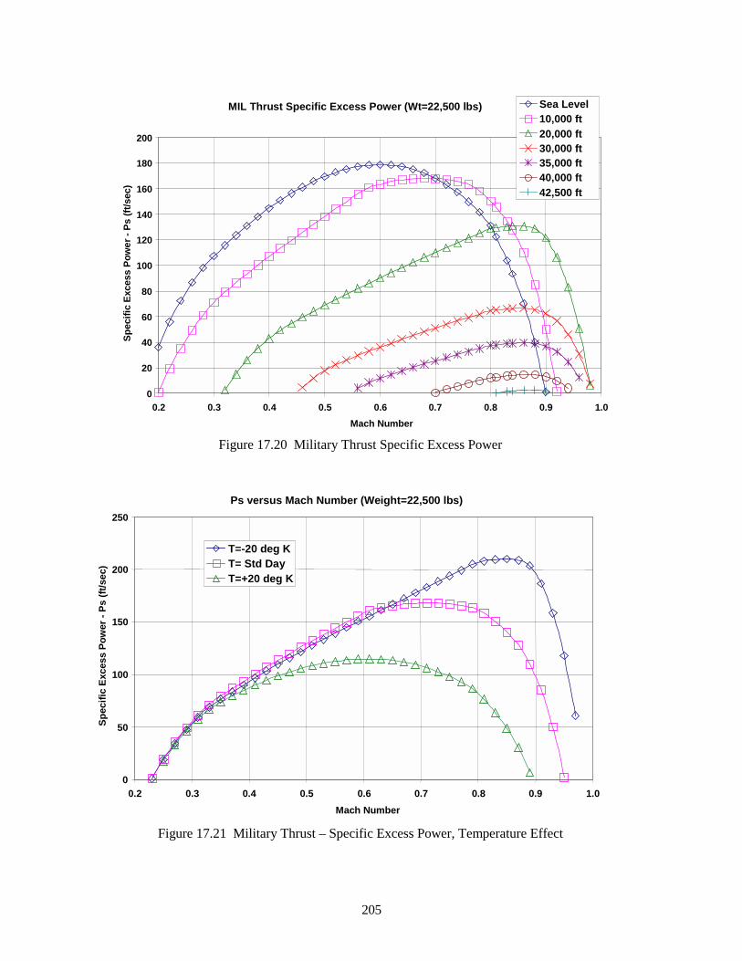
205

MIL Thrust Specific Excess Power (Wt=22,500 lbs)

0

20

40

60

80

100

120

140

160

180

200

0.2 0.3 0.4 0.5 0.6 0.7 0.8 0.9 1.0Mach Number

Spec

ific

Exce

ss P

ower

- Ps

(ft/s

ec)


Figure 17.20 Military Thrust Specific Excess Power

Ps versus Mach Number (Weight=22,500 lbs)

0

50

100

150

200

250

0.2 0.3 0.4 0.5 0.6 0.7 0.8 0.9 1.0Mach Number

Spec

ific

Exce

ss P

ower

- Ps

(ft/s

ec)

T=-20 deg KT= Std DayT=+20 deg K

Figure 17.21 Military Thrust – Specific Excess Power, Temperature Effect

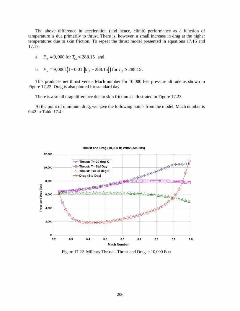
206

The above difference in acceleration (and hence, climb) performance as a function of temperature is due primarily to thrust. There is, however, a small increase in drag at the higher temperatures due to skin friction. To repeat the thrust model presented in equations 17.16 and 17.17:

a. 29,000 for 288.15nr tF T= < , and

b. [ ]( )2 29,000 1 0.01 288.15 for 288.15nr t tF T T= ⋅ − ⋅ − ≥ .

This produces net thrust versus Mach number for 10,000 feet pressure altitude as shown in Figure 17.22. Drag is also plotted for standard day.

There is a small drag difference due to skin friction as illustrated in Figure 17.23.

At the point of minimum drag, we have the following points from the model. Mach number is 0.42 in Table 17.4.

Thrust and Drag (10,000 ft; Wt=22,500 lbs)

0

2,000

4,000

6,000

8,000

10,000

12,000

0.2 0.3 0.4 0.5 0.6 0.7 0.8 0.9 1.0

Mach Number

Thru

st a

nd D

rag

(lbs)

Thrust: T=-20 deg KThrust: T= Std DayThrust: T=+20 deg KDrag (Std Day)

Figure 17.22 Military Thrust – Thrust and Drag at 10,000 Feet

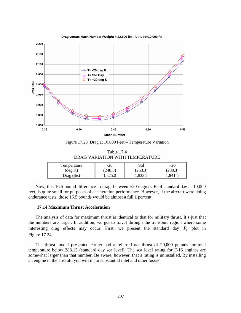
207

Drag versus Mach Number (Weight = 22,500 lbs; Altitude=10,000 ft)

1,800

1,850

1,900

1,950

2,000

2,050

2,100

2,150

2,200

0.35 0.40 0.45 0.50 0.55

Mach Number

Dra

g (lb

s)

T= -20 deg KT= Std DayT= +20 deg K

Figure 17.23 Drag at 10,000 Feet – Temperature Variation

Table 17.4 DRAG VARIATION WITH TEMPERATURE

Temperature (deg K)

-20 (248.3)

Std (268.3)

+20 (288.3)

Drag (lbs) 1,825.0 1,833.5 1,841.5

Now, this 16.5-pound difference in drag, between ±20 degrees K of standard day at 10,000 feet, is quite small for purposes of acceleration performance. However, if the aircraft were doing endurance tests, those 16.5 pounds would be almost a full 1 percent.

17.14 Maximum Thrust Acceleration

The analysis of data for maximum thrust is identical to that for military thrust. It’s just that the numbers are larger. In addition, we get to travel through the transonic region where some interesting drag effects may occur. First, we present the standard day sP plot in Figure 17.24.

The thrust model presented earlier had a referred net thrust of 20,000 pounds for total temperature below 288.15 (standard day sea level). The sea level rating for F-16 engines are somewhat larger than that number. Be aware, however, that a rating is uninstalled. By installing an engine in the aircraft, you will incur substantial inlet and other losses.

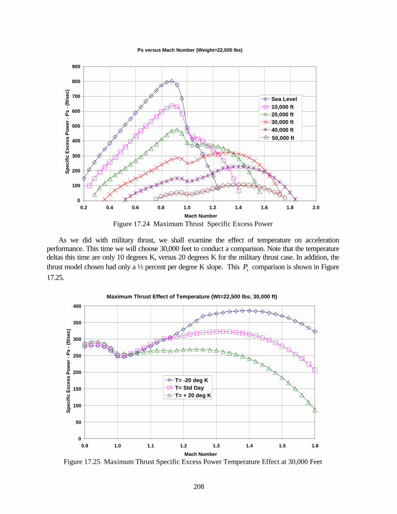
208

Ps versus Mach Number (Weight=22,500 lbs)

0

100

200

300

400

500

600

700

800

900

0.2 0.4 0.6 0.8 1.0 1.2 1.4 1.6 1.8 2.0Mach Number

Spec

ific

Exce

ss P

ower

- Ps

- (ft

/sec

)


Figure 17.24 Maximum Thrust Specific Excess Power

As we did with military thrust, we shall examine the effect of temperature on acceleration performance. This time we will choose 30,000 feet to conduct a comparison. Note that the temperature deltas this time are only 10 degrees K, versus 20 degrees K for the military thrust case. In addition, the thrust model chosen had only a ½ percent per degree K slope. This sP comparison is shown in Figure 17.25.

Maximum Thrust Effect of Temperature (Wt=22,500 lbs; 30,000 ft)

0

50

100

150

200

250

300

350

400

0.9 1.0 1.1 1.2 1.3 1.4 1.5 1.6Mach Number

Spec

ific

Exce

ss P

ower

- Ps

- (ft

/sec

)

T= -20 deg KT= Std DayT= + 20 deg K

Figure 17.25 Maximum Thrust Specific Excess Power Temperature Effect at 30,000 Feet

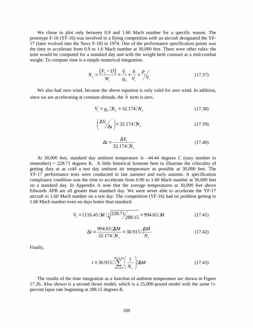
209

We chose to plot only between 0.9 and 1.60 Mach number for a specific reason. The prototype F-16 (YF-16) was involved in a flying competition with an aircraft designated the YF-17 (later evolved into the Navy F-18) in 1974. One of the performance specification points was the time to accelerate from 0.9 to 1.6 Mach number at 30,000 feet. There were other rules: the time would be computed for a standard day and with the weight held constant at a mid-combat weight. To compute time is a simple numerical integration.

( )

0

n t sx

tt t

F D V h PN VW g V−

= = + =!!

(17.37)

We also had zero wind, because the above equation is only valid for zero wind. In addition, since we are accelerating at constant altitude, the h! term is zero.

0 32.174t x xV g N N= ⋅ = ⋅! (17.38)

32.174tx

V Nt∆ = ⋅ ∆

(17.39)

32.174

t

x

VtN

∆∆ =⋅

(17.40)

At 30,000 feet, standard day ambient temperature is –44.44 degrees C (easy number to remember) = 228.71 degrees K. A little historical footnote here to illustrate the criticality of getting data at as cold a test day ambient air temperature as possible at 30,000 feet. The YF-17 performance tests were conducted in late summer and early autumn. A specification compliance condition was the time to accelerate from 0.90 to 1.60 Mach number at 30,000 feet on a standard day. In Appendix A note that the average temperatures at 30,000 feet above Edwards AFB are all greater than standard day. We were never able to accelerate the YF-17 aircraft to 1.60 Mach number on a test day. The competition (YF-16) had no problem getting to 1.60 Mach number even on days hotter than standard.

228.711116.45 994.65288.15tV M M= ⋅ ⋅ = ⋅ (17.41)

994.65 30.91532.174 x x

M MtN N

⋅∆ ∆∆ = = ⋅⋅

(17.42)

Finally,

1.60

0.9

130.915M

M x

t MN

=

=

= ⋅ ⋅∆

∑ (17.43)

The results of the time integration as a function of ambient temperature are shown in Figure 17.26. Also shown is a second thrust model, which is a 25,000-pound model with the same ½-percent lapse rate beginning at 288.15 degrees K.

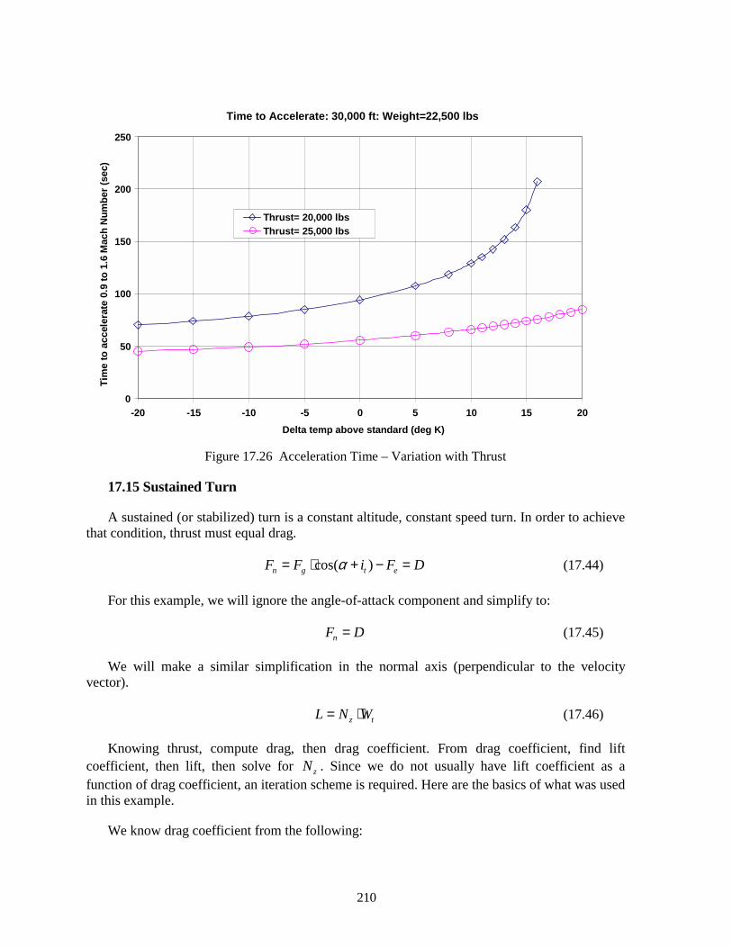
210

Time to Accelerate: 30,000 ft: Weight=22,500 lbs

0

50

100

150

200

250

-20 -15 -10 -5 0 5 10 15 20Delta temp above standard (deg K)

Tim

e to

acc

eler

ate

0.9

to 1

.6 M

ach

Num

ber (

sec)

Thrust= 20,000 lbsThrust= 25,000 lbs

Figure 17.26 Acceleration Time – Variation with Thrust

17.15 Sustained Turn

A sustained (or stabilized) turn is a constant altitude, constant speed turn. In order to achieve that condition, thrust must equal drag.

cos( )n g t eF F i F Dα= ⋅ + − = (17.44)

For this example, we will ignore the angle-of-attack component and simplify to:

nF D= (17.45)

We will make a similar simplification in the normal axis (perpendicular to the velocity vector).

z tL N W= ⋅ (17.46)

Knowing thrust, compute drag, then drag coefficient. From drag coefficient, find lift coefficient, then lift, then solve for zN . Since we do not usually have lift coefficient as a function of drag coefficient, an iteration scheme is required. Here are the basics of what was used in this example.

We know drag coefficient from the following:

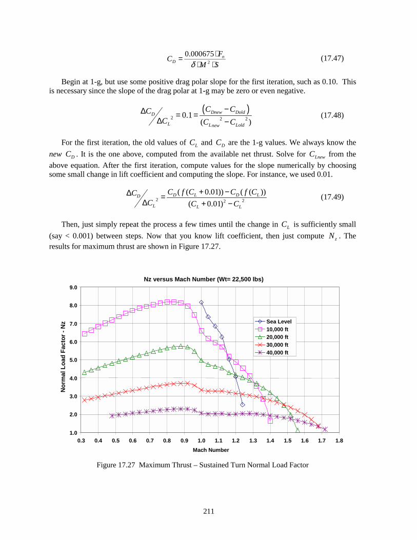
211

2

0.000675 nD

FCM Sδ

⋅=⋅ ⋅

(17.47)

Begin at 1-g, but use some positive drag polar slope for the first iteration, such as 0.10. This is necessary since the slope of the drag polar at 1-g may be zero or even negative.

( )

2 2 20.1( )

Dnew DoldD

L L Loldnew

C CCC C C

−∆ = =∆ −

(17.48)

For the first iteration, the old values of LC and DC are the 1-g values. We always know the new DC . It is the one above, computed from the available net thrust. Solve for LnewC from the above equation. After the first iteration, compute values for the slope numerically by choosing some small change in lift coefficient and computing the slope. For instance, we used 0.01.

2 22

( ( 0.01)) ( ( ))( 0.01)

D L D LD

L L L

C f C C f CCC C C

+ −∆ =∆ + −

(17.49)

Then, just simply repeat the process a few times until the change in LC is sufficiently small (say < 0.001) between steps. Now that you know lift coefficient, then just compute zN . The results for maximum thrust are shown in Figure 17.27.

Nz versus Mach Number (Wt= 22,500 lbs)

1.0

2.0

3.0

4.0

5.0

6.0

7.0

8.0

9.0

0.3 0.4 0.5 0.6 0.7 0.8 0.9 1.0 1.1 1.2 1.3 1.4 1.5 1.6 1.7 1.8Mach Number

Nor

mal

Loa

d Fa

ctor

- N

z Sea Level10,000 ft20,000 ft30,000 ft40,000 ft

Figure 17.27 Maximum Thrust – Sustained Turn Normal Load Factor

212

The constraints imposed on this turn problem were the following.

a. maxL LC C< ,

b. max 1.50LC = ,

c. maxz zN N< , and

d. max 9.0zN = .

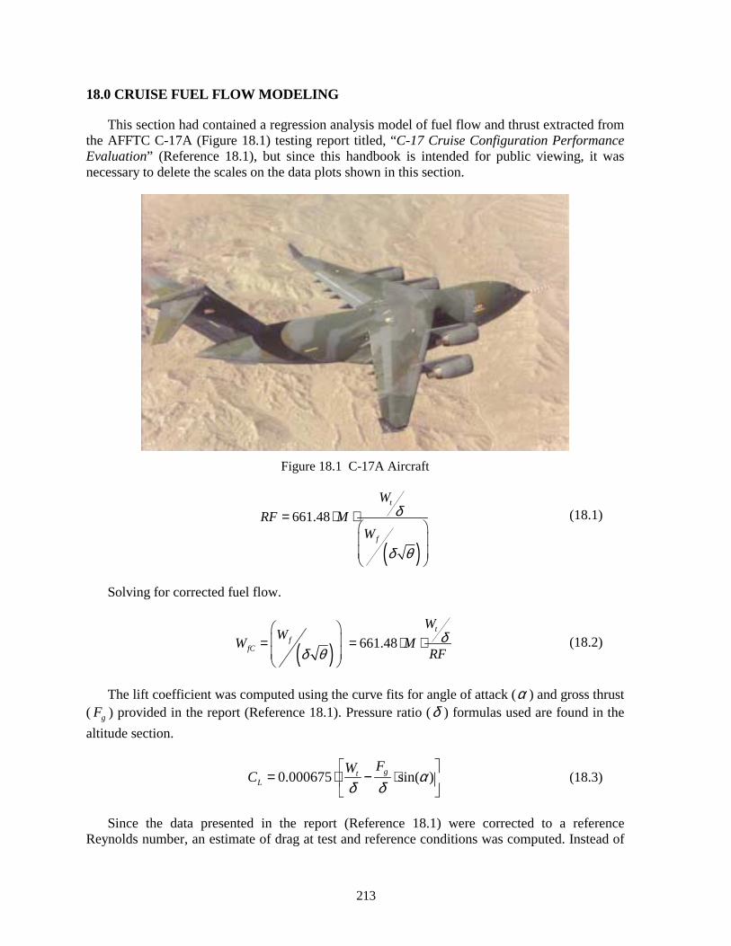
213

18.0 CRUISE FUEL FLOW MODELING

This section had contained a regression analysis model of fuel flow and thrust extracted from the AFFTC C-17A (Figure 18.1) testing report titled, “C-17 Cruise Configuration Performance Evaluation” (Reference 18.1), but since this handbook is intended for public viewing, it was necessary to delete the scales on the data plots shown in this section.

Figure 18.1 C-17A Aircraft

( )661.48

t

f

WRF M

Wδ

δ θ

= ⋅ ⋅

(18.1)

Solving for corrected fuel flow.

( ) 661.48t

ffC

WWW M

RFδ

δ θ

= = ⋅ ⋅

(18.2)

The lift coefficient was computed using the curve fits for angle of attack (α ) and gross thrust ( gF ) provided in the report (Reference 18.1). Pressure ratio (δ ) formulas used are found in the altitude section.

0.000675 sin( )gtL

FWC αδ δ

= ⋅ − ⋅

(18.3)

Since the data presented in the report (Reference 18.1) were corrected to a reference Reynolds number, an estimate of drag at test and reference conditions was computed. Instead of

214

the usual ‘standardization’ we are essentially ‘un-standardizing’ the drag data. We are going from a reference condition to a standard condition. The formulas used are those presented in the lift and drag section.

The reference wing area ( S ) and the wetted area ( wetS ) are as follows:

a. S =3,800. ft2, and

b. wetS =19,075. ft2.

Skin friction drag relationships are as follows:

2.58100.455 / log ( )fC RN= (18.4)

2 0.65/(1 0.144 )fC fC C M= + ⋅ (18.5)

wetD fCf

SC CS

= ⋅ (18.6)

The assumption was made that the characteristic length used was the mean aerodynamic chord ( MAC ). That value is as follows:

l MAC= = 25.794 feet.

To perform a curve fit of the fuel flow data, we will remove the skin friction drag correction from the thrust data. The standard day drag coefficient ( DsC ) was computed from the drag polar curve fit formulas in the report. The drag coefficient formula in the report was referenced to a Reynolds number of 1,800,000 per foot. The test day drag coefficient ( DtC ) was computed as follows:

( )tD Ds Dft DfsC C C C= + − (18.7)

The standard (or reference) skin friction drag coefficient is based upon the standard Reynolds number per foot and the characteristic length. Inserting these numbers into equation 18.4:

2.58100.455 / log (1,800,000 25.794)fsC = ⋅ = 0.00238 (18.8)

From a formula defined in the lift and drag section,

( )

2

110398.15T

RNI δθ

+ = ⋅

(18.9)

67.101 10RN M RNI l= ⋅ ⋅ ⋅ ⋅

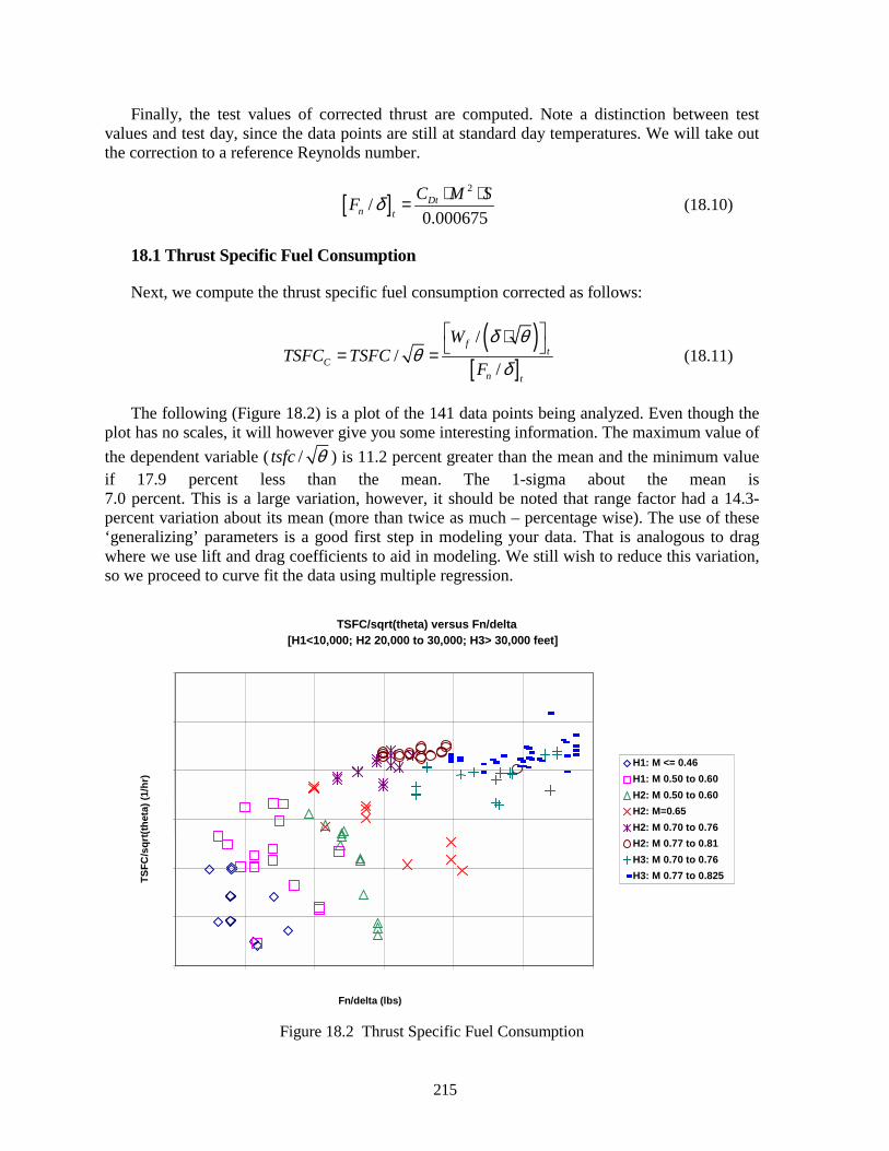
215

Finally, the test values of corrected thrust are computed. Note a distinction between test values and test day, since the data points are still at standard day temperatures. We will take out the correction to a reference Reynolds number.

[ ]2

/0.000675

Dtn t

C M SF δ ⋅ ⋅= (18.10)

18.1 Thrust Specific Fuel Consumption

Next, we compute the thrust specific fuel consumption corrected as follows:

( )

[ ]/

//

ft

Cn t

WTSFC TSFC

F

δ θθ

δ

⋅ = = (18.11)

The following (Figure 18.2) is a plot of the 141 data points being analyzed. Even though the plot has no scales, it will however give you some interesting information. The maximum value of the dependent variable ( /tsfc θ ) is 11.2 percent greater than the mean and the minimum value if 17.9 percent less than the mean. The 1-sigma about the mean is 7.0 percent. This is a large variation, however, it should be noted that range factor had a 14.3-percent variation about its mean (more than twice as much – percentage wise). The use of these ‘generalizing’ parameters is a good first step in modeling your data. That is analogous to drag where we use lift and drag coefficients to aid in modeling. We still wish to reduce this variation, so we proceed to curve fit the data using multiple regression.

TSFC/sqrt(theta) versus Fn/delta[H1<10,000; H2 20,000 to 30,000; H3> 30,000 feet]

0.52

0.56

0.60

0.64

0.68

0.72

0.76

20000 40000 60000 80000 100000 120000 140000

Fn/delta (lbs)

TSFC

/sqr

t(the

ta) (

1/hr

)

H1: M <= 0.46H1: M 0.50 to 0.60H2: M 0.50 to 0.60H2: M=0.65H2: M 0.70 to 0.76H2: M 0.77 to 0.81H3: M 0.70 to 0.76H3: M 0.77 to 0.825

Figure 18.2 Thrust Specific Fuel Consumption

216

18.2 Multiple Regression

Now, we will strive to develop an equation that fits the data presented in Figure 18.2. The simplest possible equation is a constant. We will use Reynolds number index ( RNI ) as an altitude parameter. In general, the formula will be as follows:

( )( )/ / , ,nTSFC f F M RNIθ δ= (18.12)

For ease of representation, we will make the following variable name changes:

a. /Y TSFC θ= ,

b. 1 /nX F δ= ,

c. 2X M= , and

d. 3X RNI= .

Then, equivalently:

( )1, 2, 3Y f X X X= (18.13)

The author used MS Excel to evaluate the data. Excel has matrix operators, however it was necessary to develop a multiple regression method for use with Excel. For those who do not have a multiple regression program available, the following is the formulation for multiple regression.

The general case for linear multiple regression:

0 1 1 2 2 m mY a a X a X a X= + ⋅ + ⋅ + + ⋅# (18.14)

The coefficients are solved by the following:

11, 2, ,

02

1, 1, 2, 1, 1, , 1,12

2 2,2, 2, 1, 2, 2, ,

2,, , 1, , 2, ,

i i m i i

i i i i i m i i i

i ii i i i i m i

mm i im i m i i m i i m i

N X X X YaX X X X X X X Ya

a X YX X X X X X

a X YX X X X X X

−

⋅ ⋅ ⋅ = ⋅ ⋅⋅ ⋅ ⋅⋅ ⋅

∑ ∑ ∑ ∑∑ ∑ ∑ ∑ ∑

∑∑ ∑ ∑ ∑

∑∑ ∑ ∑ ∑

#

#

#$ $$ $ $ $

#

(18.15)

where:

N = number of data points.

The above general curve fit formula was developed by minimizing the sum of the squares of the residual errors ( SS ). The formula for SS is as follows:

217

( )2ˆi iSS Y Y= −∑ (18.16)

where:

Y = the curve fit equation.

There are a number of ways to evaluate the quality of a curve fit. We will look at the standard deviation.

/( 1)SS Nσ = − (18.17)

A percentage standard deviation will be calculated,

% ( / ) 100Yσ σ= ⋅ (18.18)

where:

Y = the mean value of the independent variable.

Here are the results of the curve fits:

a. 0Y a= % 7.00%σ = ,

b. 0 1ˆ 1Y a a X= + ⋅ % 5.30%σ = , and

c. 20 1 2

ˆ 1 1Y a a X a X= + ⋅ + ⋅ % 5.16%σ = .

At this point, we should pause to examine the residual errors rather than just blindly adding additional terms to the equation. From Figure 18.3, we can see some apparent additional Mach number and Reynolds number effects. So far, we have only reduced the 1-sigma about the mean from 7.0 percent to 5.16 percent. This is a disappointing result; however, we suspect there may be a substantial altitude and Mach number effect. The parameter we will plot is the percentage error as follows:

( )ˆ%100YError Y Y = − ⋅

(18.19)

The Y used will be from the last curve fit (equation 18.18).

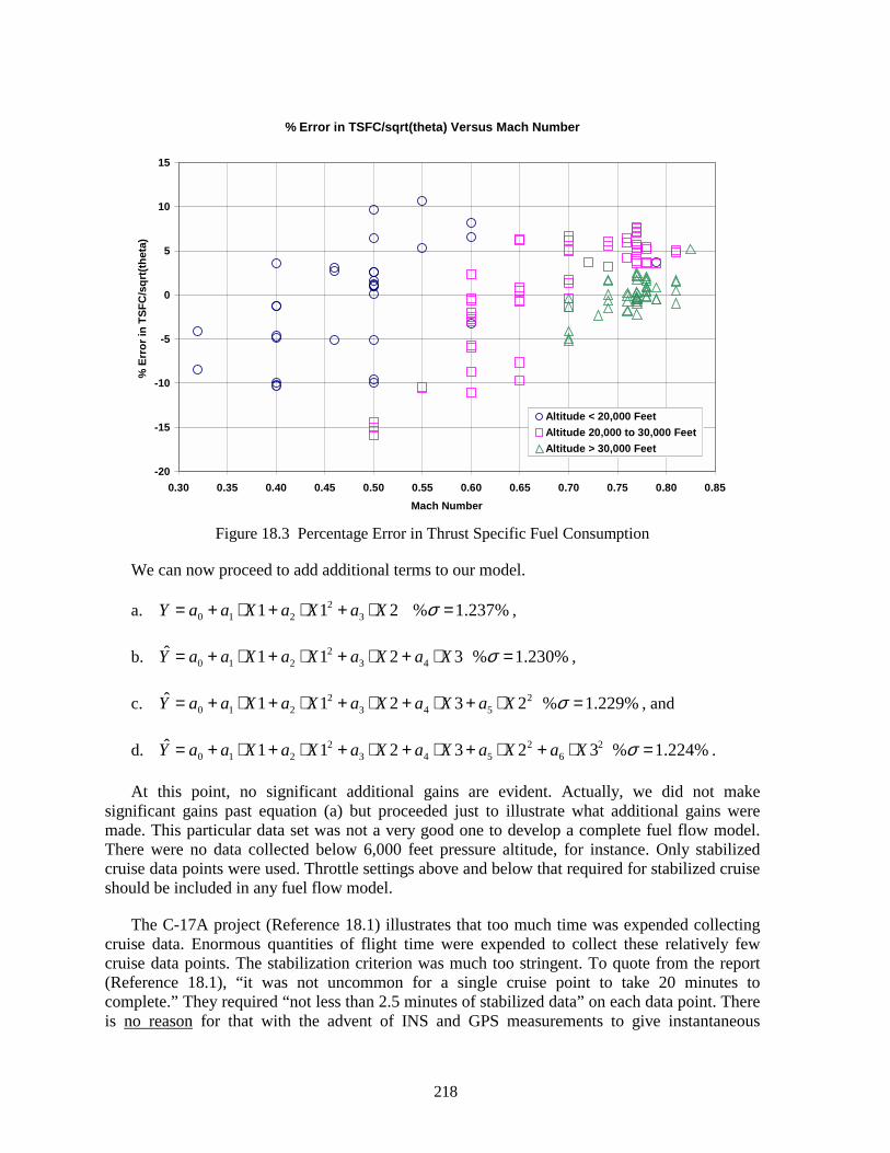
218

% Error in TSFC/sqrt(theta) Versus Mach Number

-20

-15

-10

-5

0

5

10

15

0.30 0.35 0.40 0.45 0.50 0.55 0.60 0.65 0.70 0.75 0.80 0.85Mach Number

% E

rror

in T

SFC

/sqr

t(the

ta)

Altitude < 20,000 FeetAltitude 20,000 to 30,000 FeetAltitude > 30,000 Feet

Figure 18.3 Percentage Error in Thrust Specific Fuel Consumption

We can now proceed to add additional terms to our model.

a. 20 1 2 31 1 2Y a a X a X a X= + ⋅ + ⋅ + ⋅ % 1.237%σ = ,

b. 20 1 2 3 4

ˆ 1 1 2 3Y a a X a X a X a X= + ⋅ + ⋅ + ⋅ + ⋅ % 1.230%σ = ,

c. 2 20 1 2 3 4 5

ˆ 1 1 2 3 2Y a a X a X a X a X a X= + ⋅ + ⋅ + ⋅ + ⋅ + ⋅ % 1.229%σ = , and

d. 2 2 20 1 2 3 4 5 6

ˆ 1 1 2 3 2 3Y a a X a X a X a X a X a X= + ⋅ + ⋅ + ⋅ + ⋅ + ⋅ + ⋅ % 1.224%σ = .

At this point, no significant additional gains are evident. Actually, we did not make significant gains past equation (a) but proceeded just to illustrate what additional gains were made. This particular data set was not a very good one to develop a complete fuel flow model. There were no data collected below 6,000 feet pressure altitude, for instance. Only stabilized cruise data points were used. Throttle settings above and below that required for stabilized cruise should be included in any fuel flow model.

The C-17A project (Reference 18.1) illustrates that too much time was expended collecting cruise data. Enormous quantities of flight time were expended to collect these relatively few cruise data points. The stabilization criterion was much too stringent. To quote from the report (Reference 18.1), “it was not uncommon for a single cruise point to take 20 minutes to complete.” They required “not less than 2.5 minutes of stabilized data” on each data point. There is no reason for that with the advent of INS and GPS measurements to give instantaneous

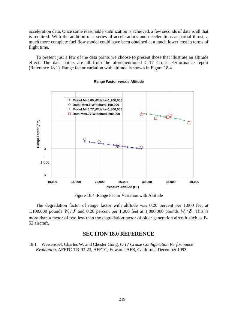
219

acceleration data. Once some reasonable stabilization is achieved, a few seconds of data is all that is required. With the addition of a series of accelerations and decelerations at partial thrust, a much more complete fuel flow model could have been obtained at a much lower cost in terms of flight time.

To present just a few of the data points we choose to present those that illustrate an altitude effect. The data points are all from the aforementioned C-17 Cruise Performance report (Reference 18.1). Range factor variation with altitude is shown in Figure 18.4.

Range Factor versus Altitude

9000

10000

11000

12000

10,000 15,000 20,000 25,000 30,000 35,000 40,000Pressure Altitude (FT)

Ran

ge F

acto

r (nm

)

Model:M=0.60;W/delta=1,100,000Data: M=0.6;W/delta=1,100,000Model:M=0.77;W/delta=1,800,000Data:M=0.77;W/delta=1,800,000

1,000

Figure 18.4 Range Factor Variation with Altitude

The degradation factor of range factor with altitude was 0.20 percent per 1,000 feet at 1,100,000 pounds /tW δ and 0.26 percent per 1,000 feet at 1,800,000 pounds /tW δ . This is more than a factor of two less than the degradation factor of older generation aircraft such as B-52 aircraft.

SECTION 18.0 REFERENCE

18.1 Weisenseel, Charles W. and Chester Gong, C-17 Cruise Configuration Performance Evaluation, AFFTC-TR-93-23, AFFTC, Edwards AFB, California, December 1993.

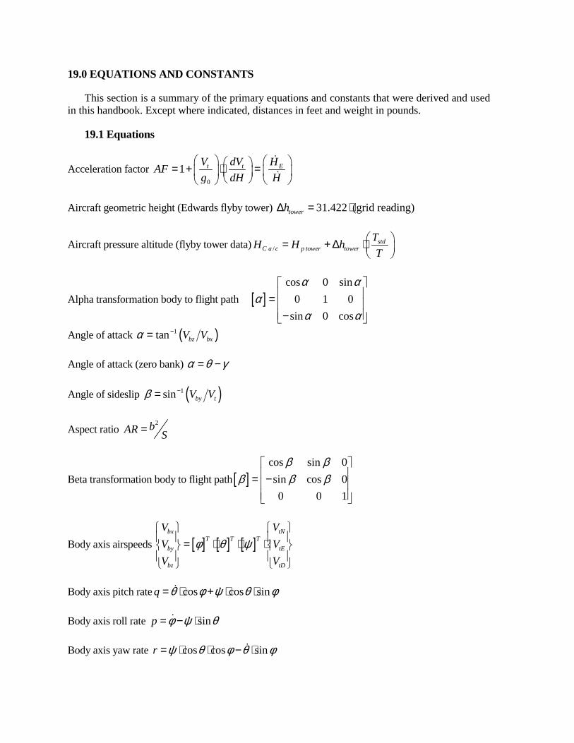
19.0 EQUATIONS AND CONSTANTS

This section is a summary of the primary equations and constants that were derived and used in this handbook. Except where indicated, distances in feet and weight in pounds.

19.1 Equations

Acceleration factor 0

1 t t EV dV HAFg dH H

= + ⋅ =

!!

Aircraft geometric height (Edwards flyby tower) 31.422 (grid reading)towerh∆ = ⋅

Aircraft pressure altitude (flyby tower data) /std

C a c p tower towerTH H hT

= + ∆ ⋅

Alpha transformation body to flight path [ ]cos 0 sin

0 1 0sin 0 cos

α αα

α α

= −

Angle of attack ( )1tan bz bxV Vα −= Angle of attack (zero bank) α θ γ= − Angle of sideslip ( )1sin by tV Vβ −= Aspect ratio

2bAR S=

Beta transformation body to flight path[ ]cos sin 0sin cos 00 0 1

β ββ β β

= −

Body axis airspeeds [ ] [ ] [ ]bx tN

T T Tby tE

bz tD

V VV VV V

φ θ ψ = ⋅ ⋅ ⋅

Body axis pitch rate cos cos sinq θ φ ψ θ φ= ⋅ + ⋅ ⋅! ! Body axis roll rate sinp φ ψ θ= − ⋅! ! Body axis yaw rate cos cos sinr ψ θ φ θ φ= ⋅ ⋅ − ⋅!!

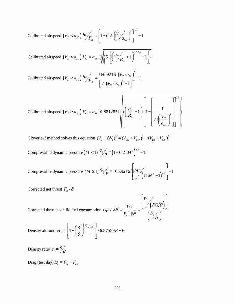
221

Calibrated airspeed ( )C SLV a<3.52

1 0.2 1C C

SL SL

q VP a

= + ⋅ −

Calibrated airspeed ( )C SLV a<(1 3.5)

5 1 1CC SL

SL

qV a P = ⋅ ⋅ + −

Calibrated airspeed ( )C SLV a≥( )

( )

7

2.52

166.92161

7 1

C SLC

SLC SL

V aqP

V a

⋅= − ⋅ −

Calibrated airspeed ( )C SLV a≥

2.5

210.881285 1 1

7

CC SL

SL C

SL

qV aP V

a

= ⋅ ⋅ + ⋅ − ⋅

Cloverleaf method solves this equation 2 2 2( ) ( ) ( )ti t gN wN gE wEV V V V V V+ ∆ = + + +

Compressible dynamic pressure ( )1M < ( )3.521 0.2 1cq MP = + ⋅ −

Compressible dynamic pressure ( 1)M ≥( )

72.52

166.9216 17 1

Cq MP M

= ⋅ − ⋅ −

Corrected net thrust /nF δ

Corrected thrust specific fuel consumption ( )

/

f

f

nn

W

Wtsfc

FF

δ θθ

θδ

⋅ = =

⋅

Density altitude ( )1

4.25591 / 6.87559 6dH Eδ

θ

= − −

Density ratio δσ θ=

Drag (test day) t nt extD F F= −

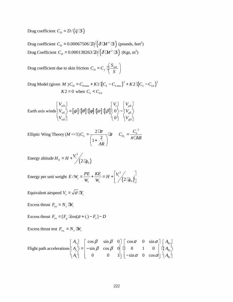
222

Drag coefficient ( )/DC D q S= ⋅ Drag coefficient ( )20.00067506DC D M Sδ= ⋅ ⋅ ⋅ (pounds, feet2)

Drag Coefficient ( )20.000138263DC D M Sδ= ⋅ ⋅ ⋅ (Kgs, m2)

Drag coefficient due to skin friction wetD f

SC CS

= ⋅

Drag Model (given M ) ( ) ( )2 2

min min1 2D D L L L LbC C K C C K C C= + ⋅ − + ⋅ −

2 0K = when L LbC C<

Earth axis winds [ ] [ ] [ ] [ ] [ ] 00

wN t gN

wE gE

wD gD

V V VV VV V

ψ θ φ α β = ⋅ ⋅ ⋅ ⋅ −

Elliptic Wing Theory (M <<1)22

21L

LL D

CC CAR

AR

π απ

⋅= ⋅ =⋅ +

Energy altitude ( )2

02t

EVH H g= + ⋅

Energy per unit weight ( )2

0/ 2

tt

t t

PE KE VE W H gW W = + = + ⋅

Equivalent airspeed e tV Vσ= ⋅ Excess thrust ex x tF N W= ⋅ Excess thrust [ cos( ) ]ex g t eF F i F Dα= ⋅ + − − Excess thrust test

tex x tF N W= ⋅

Flight path accelerationscos sin 0 cos 0 sinsin cos 0 0 1 00 0 1 sin 0 cos

x bx

y by

z bz

A AA AA A

β β α αβ β

α α

= − ⋅ ⋅ −

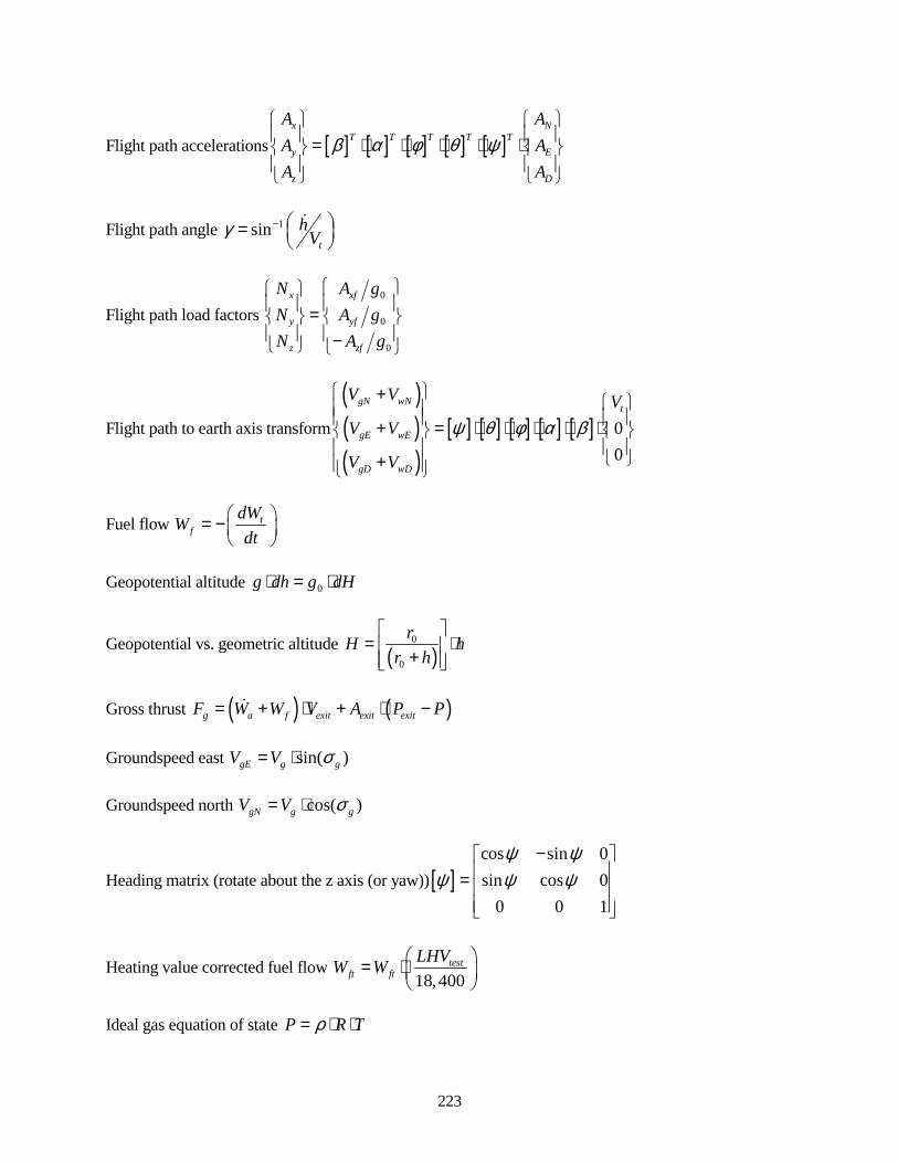
223

Flight path accelerations [ ] [ ] [ ] [ ] [ ]x N

T T T T Ty E

z D

A AA AA A

β α φ θ ψ = ⋅ ⋅ ⋅ ⋅ ⋅

Flight path angle 1sint

hVγ − =

!

Flight path load factors 0

0

0

x xf

y yf

z zf

N A gN A gN A g

=

−

Flight path to earth axis transform

( )( )( )

[ ] [ ] [ ] [ ] [ ] 00

gN wNt

gE wE

gD wD

V V VV V

V V

ψ θ φ α β

+ + = ⋅ ⋅ ⋅ ⋅ ⋅

+

Fuel flow tf

dWWdt

= −

Geopotential altitude 0g dh g dH⋅ = ⋅

Geopotential vs. geometric altitude ( )

0

0

rH hr h

= ⋅ +

Gross thrust ( ) ( )g a f exit exit exitF W W V A P P= + ⋅ + ⋅ −! Groundspeed east sin( )gE g gV V σ= ⋅ Groundspeed north cos( )gN g gV V σ= ⋅

Heading matrix (rotate about the z axis (or yaw))[ ]cos sin 0sin cos 0

0 0 1

ψ ψψ ψ ψ

− =

Heating value corrected fuel flow 18,400

testft ft

LHVW W = ⋅

Ideal gas equation of state P R Tρ= ⋅ ⋅

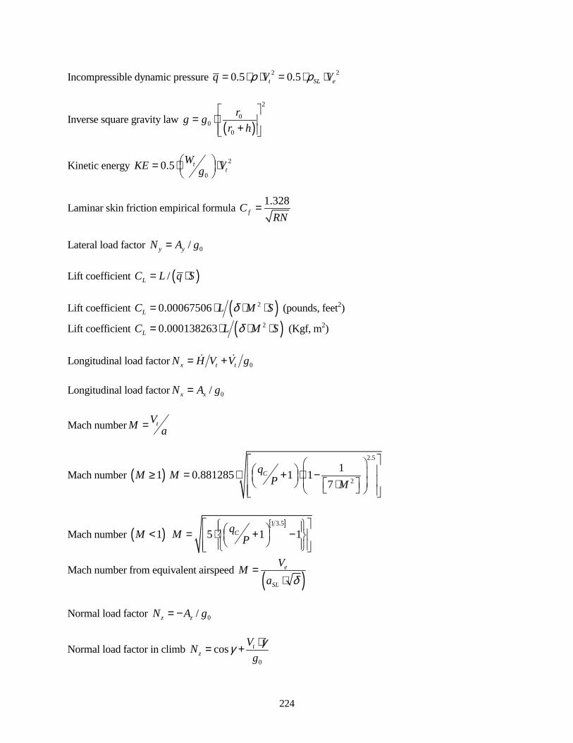
224

Incompressible dynamic pressure 2 20.5 0.5t SL eq V Vρ ρ= ⋅ ⋅ = ⋅ ⋅

Inverse square gravity law ( )

2

00

0

rg gr h

= ⋅ +

Kinetic energy 2

00.5 t

tWKE Vg = ⋅ ⋅

Laminar skin friction empirical formula 1.328fC

RN=

Lateral load factor 0/y yN A g= Lift coefficient ( )/LC L q S= ⋅ Lift coefficient ( )20.00067506LC L M Sδ= ⋅ ⋅ ⋅ (pounds, feet2)

Lift coefficient ( )20.000138263LC L M Sδ= ⋅ ⋅ ⋅ (Kgf, m2) Longitudinal load factor 0x t tN H V V g= +! ! Longitudinal load factor 0/x xN A g=

Mach number tVM a=

Mach number ( )1M ≥

2.5

2

10.881285 1 17

CqM P M

= ⋅ + ⋅ − ⋅

Mach number ( )1M < [ ]1 3.5

5 1 1CqM P = ⋅ + −

Mach number from equivalent airspeed ( )e

SL

VMa δ

=⋅

Normal load factor 0/z zN A g= −

Normal load factor in climb 0

cos tz

VNgγγ ⋅= +!

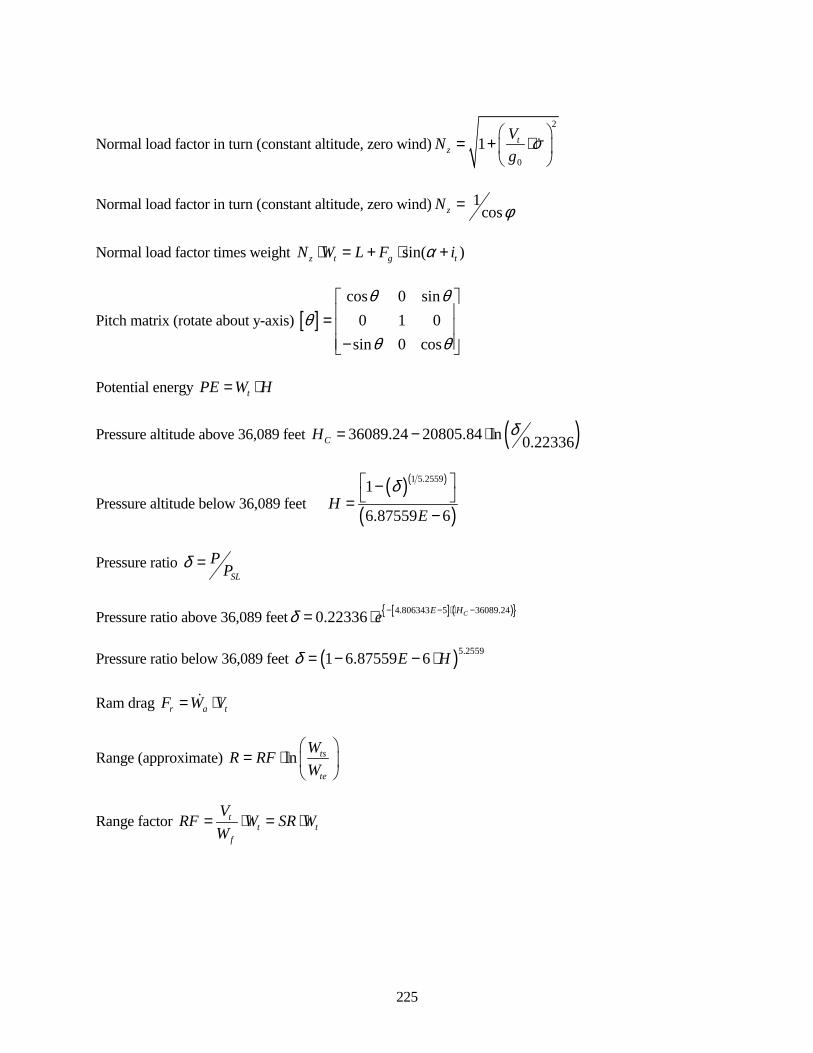
225

Normal load factor in turn (constant altitude, zero wind)2

0

1 tz

VNg

σ

= + ⋅

!

Normal load factor in turn (constant altitude, zero wind) 1

coszN φ=

Normal load factor times weight sin( )z t g tN W L F iα⋅ = + ⋅ +

Pitch matrix (rotate about y-axis) [ ]cos 0 sin

0 1 0sin 0 cos

θ θθ

θ θ

= −

Potential energy tPE W H= ⋅ Pressure altitude above 36,089 feet ( )36089.24 20805.84 ln 0.22336CH δ= − ⋅

Pressure altitude below 36,089 feet ( )( )

( )

1 5.25591

6.87559 6H

E

δ − =−

Pressure ratio

SL

PPδ =

Pressure ratio above 36,089 feet [ ] ( ){ }4.806343 5 36089.240.22336 CE Heδ − − ⋅ −= ⋅ Pressure ratio below 36,089 feet ( )5.25591 6.87559 6E Hδ = − − ⋅ Ram drag r a tF W V= ⋅!

Range (approximate) ln ts

te

WR RFW

= ⋅

Range factor tt t

f

VRF W SR WW

= ⋅ = ⋅

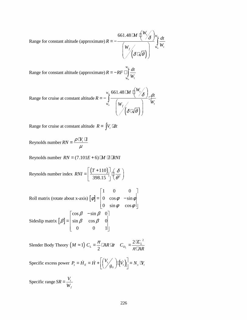
226

Range for constant altitude (approximate)

( )

661.48 te

ts

t W

tWf

WM dtRWW

δ

δ θ

⋅ ⋅ = −

⋅

∫

Range for constant altitude (approximate)te

ts

W

tW

dtR RFW

= − ⋅ ∫

Range for cruise at constant altitude

( )

661.48te

ts

tW

tWf

WM dtRWW

δ

δ θ

⋅ ⋅ = − ⋅

⋅

∫

Range for cruise at constant altitude tR V dt= ⋅∫

Reynolds number tV lRN ρµ⋅ ⋅=

Reynolds number (7.101 6)RN E M l RNI= + ⋅ ⋅ ⋅

Reynolds number index ( )

2

110398.15T

RNI δθ

+ = ⋅

Roll matrix (rotate about x-axis) [ ]1 0 00 cos sin0 sin cos

φ φ φφ φ

= −

Sideslip matrix [ ]cos sin 0sin cos 0

0 0 1

β ββ β β

− =

Slender Body Theory ( )1M ≈22

2 L

LL D

CC AR CAR

π απ⋅= ⋅ ⋅ =⋅

Specific excess power ( )0

ts E t x t

VP H H V N Vg = = + ⋅ = ⋅

! ! !

Specific range t

f

VSRW

=

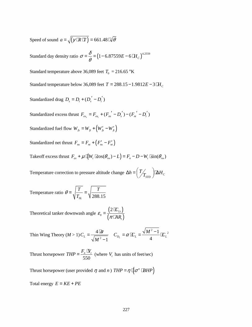
227

Speed of sound ( ) 661.48a R Tγ θ= ⋅ ⋅ = ⋅

Standard day density ratio ( )4.25591 6.87559 6 CE Hδσθ

= = − − ⋅

Standard temperature above 36,089 feet 0T = 216.65 °K Standard temperature below 36,089 feet 288.15 1.9812 3 CT E H= − − ⋅

Standardized drag ( )s t s tD D D D′ ′= + −

Standardized excess thrust ( ) ( )s tex ex ns s nt tF F F D F D′ ′ ′ ′= + − − −

Standardized fuel flow ( )fs ft fs ftW W W W′ ′= + − Standardized net thrust ( )ns nt ns ntF F F F′ ′= + − Takeoff excess thrust ( )cos( ) sin( )ex t rw n t rwF W L F D Wµ θ θ+ ⋅ ⋅ − = − − ⋅

Temperature correction to pressure altitude change CSTD

Th HT ∆ = ⋅∆

Temperature ratio 288.15SL

T TT

θ = =

Theoretical tanker downwash angle ( )( )0

2 Lt

t

CAR

επ⋅

=⋅

Thin Wing Theory (M > 1)2

2

2

4 141 LL D L L

MC C C CMα α⋅ −= = ⋅ = ⋅−

Thrust horsepower 550n tF VTHP ⋅= (where tV has units of feet/sec)

Thrust horsepower (user provided and nη ) ( )nTHP BHPη σ= ⋅ ⋅ Total energy E KE PE= +

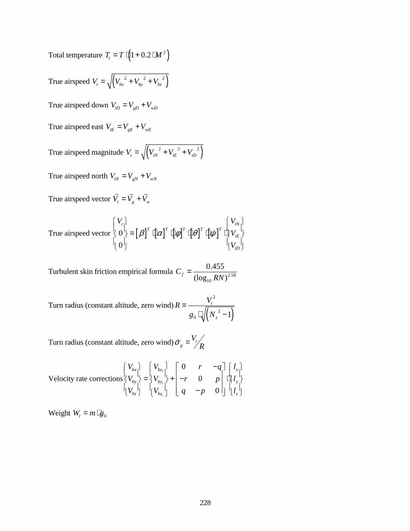
228

Total temperature ( )21 0.2tT T M= ⋅ + ⋅

True airspeed ( )2 2 2t bx by bzV V V V= + +

True airspeed down tD gD wDV V V= + True airspeed east tE gE wEV V V= +

True airspeed magnitude ( )2 2 2t tN tE tDV V V V= + +

True airspeed north tN gN wNV V V= + True airspeed vector t g wV V V= +

" " "

True airspeed vector [ ] [ ] [ ] [ ] [ ]00

t tNT T T T T

tE

tD

V VVV

β α φ θ ψ = ⋅ ⋅ ⋅ ⋅ ⋅

Turbulent skin friction empirical formula 2.5810

0.455(log )fC

RN=

Turn radius (constant altitude, zero wind)( )

2

20 1

t

z

VRg N

=⋅ −

Turn radius (constant altitude, zero wind) tg

VRσ =!

Velocity rate corrections0

00

i

i

i

bx bx x

by by y

bz bz z

V V r q lV V r p lV V q p l

− = + − ⋅

−

Weight 0tW m g= ⋅

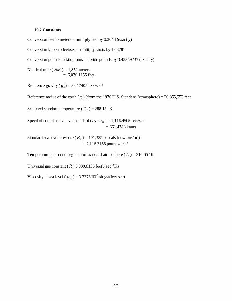
229

19.2 Constants

Conversion feet to meters = multiply feet by 0.3048 (exactly) Conversion knots to feet/sec = multiply knots by 1.68781 Conversion pounds to kilograms = divide pounds by 0.45359237 (exactly) Nautical mile ( NM ) = 1,852 meters = 6,076.1155 feet Reference gravity ( 0g ) = 32.17405 feet/sec²

Reference radius of the earth ( 0r ) (from the 1976 U.S. Standard Atmosphere) = 20,855,553 feet Sea level standard temperature ( SLT ) = 288.15 °K Speed of sound at sea level standard day ( SLa ) = 1,116.4505 feet/sec

= 661.4788 knots Standard sea level pressure ( SLP ) = 101,325 pascals (newtons/m2)

= 2,116.2166 pounds/feet² Temperature in second segment of standard atmosphere ( 0T ) = 216.65 °K Universal gas constant ( R ) 3,089.8136 feet²/(sec²°K) Viscosity at sea level ( SLµ ) = 3.7373⋅10-7 slugs/(feet sec)

230


231

APPENDIX A

AVERAGE WINDS AND TEMPERATURES FOR THE AIR FORCE FLIGHT TEST CENTER

232


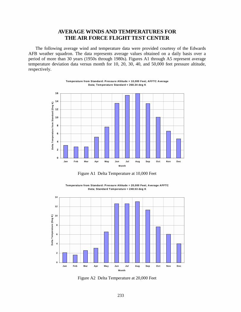
233

AVERAGE WINDS AND TEMPERATURES FOR THE AIR FORCE FLIGHT TEST CENTER

The following average wind and temperature data were provided courtesy of the Edwards AFB weather squadron. The data represents average values obtained on a daily basis over a period of more than 30 years (1950s through 1980s). Figures A1 through A5 represent average temperature deviation data versus month for 10, 20, 30, 40, and 50,000 feet pressure altitude, respectively.

Temperature from Standard: Pressure Altitude = 10,000 Feet; AFFTC Average Data; Temperature Standard = 268.34 deg K

0

2

4

6

8

10

12

14

16

Jan Feb Mar Apr May Jun Jul Aug Sep Oct Nov Dec

Month

Del

ta T

empe

ratu

re f

rom

Sta

ndar

d (D

eg K

)

Figure A1 Delta Temperature at 10,000 Feet

Temperature from Standard: Pressure Altitude = 20,000 Feet; Average AFFTC Data; Standard Temperature = 248.53 deg K

0

2

4

6

8

10

12

14


Month

Del

ta T

empe

ratu

re (

Deg

K)


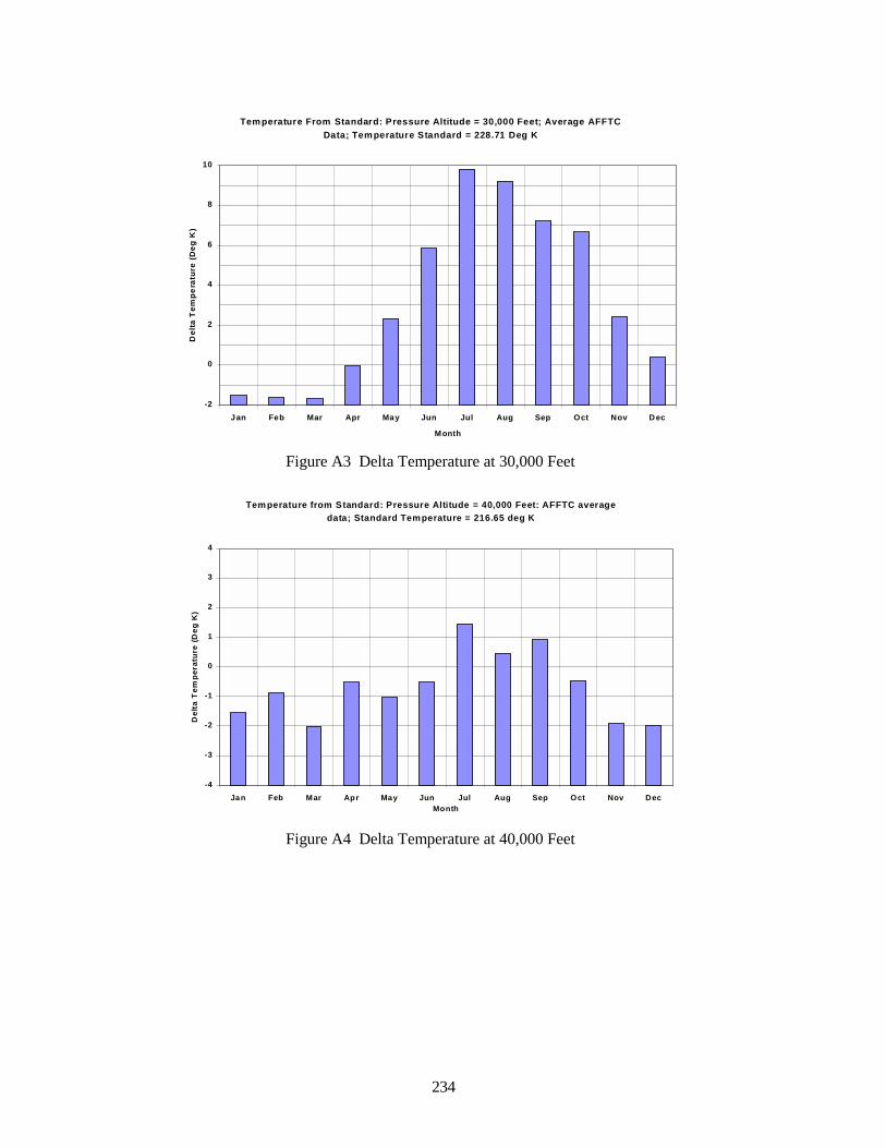
234

Temperature From Standard: Pressure Altitude = 30,000 Feet; Average AFFTC Data; Temperature Standard = 228.71 Deg K

-2

0

2

4

6

8

10


Month

Del

ta T

empe

ratu

re (

Deg

K)


Temperature from Standard: Pressure Altitude = 40,000 Feet: AFFTC average data; Standard Temperature = 216.65 deg K

-4

-3

-2

-1

0

1

2

3

4

Jan Feb Mar Apr May Jun Jul Aug Sep Oct Nov DecMonth

Del

ta T

empe

ratu

re (D

eg K

)


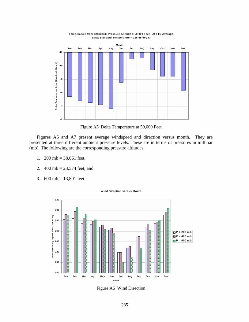
235

Temperature from Standard: Pressure Altitude = 50,000 Feet : AFFTC Average data; Standard Tem perature = 216.65 deg K

-12

-10

-8

-6

-4

-2

Jan Feb Mar Apr May Jun Jul Aug Sep Oct Nov DecMonth

Del

ta T

empe

ratu

re fr

om S

tand

ard

(Deg

K)


Figures A6 and A7 present average windspeed and direction versus month. They are presented at three different ambient pressure levels. These are in terms of pressures in millibar (mb). The following are the corresponding pressure altitudes:

1. 200 mb = 38,661 feet,

2. 400 mb = 23,574 feet, and

3. 600 mb = 13,801 feet.

Wind Direction versus Month

180

200

220

240

260

280

300

320


Month

Win

d D

irec

tion

(Deg

rees

from

Tru

e N

ort

h)

P = 200 mbP = 400 mbP = 600 mb

Figure A6 Wind Direction

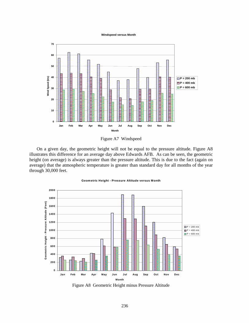
236

Windspeed versus Month

0

10

20

30

40

50

60

70


Month

Win

d Sp

eed

(kts

)

P = 200 mbP = 400 mbP = 600 mb

Figure A7 Windspeed

On a given day, the geometric height will not be equal to the pressure altitude. Figure A8 illustrates this difference for an average day above Edwards AFB. As can be seen, the geometric height (on average) is always greater than the pressure altitude. This is due to the fact (again on average) that the atmospheric temperature is greater than standard day for all months of the year through 30,000 feet.

Geometric Height - Pressure Altitude versus M onth

0

200

400

600

800

1000

1200

1400

1600

1800

2000


Month

Geo

met

ric

Hei

ght

- Pre

ssu

re A

ltitu

de (F

eet)

P = 200 m bP = 400 m bP = 600 m b

Figure A8 Geometric Height minus Pressure Altitude

237

APPENDIX B

WEATHER TIME HISTORIES

238


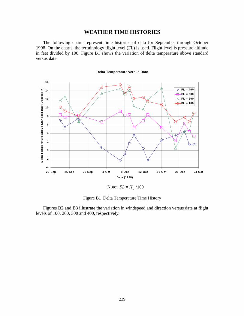
239

WEATHER TIME HISTORIES

The following charts represent time histories of data for September through October 1998. On the charts, the terminology flight level (FL) is used. Flight level is pressure altitude in feet divided by 100. Figure B1 shows the variation of delta temperature above standard versus date.

Delta Temperature versus Date

-4

-2

0

2

4

6

8

10

12

14

16

22-Sep 26-Sep 30-Sep 4-Oct 8-Oct 12-Oct 16-Oct 20-Oct 24-Oct

Date (1998)

Del

ta T

empe

ratu

re A

bove

Sta

nda

rd D

ay (

Deg

rees

K)

FL = 400FL = 300FL = 200FL = 100

Note: /100CFL H=

Figure B1 Delta Temperature Time History

Figures B2 and B3 illustrate the variation in windspeed and direction versus date at flight levels of 100, 200, 300 and 400, respectively.

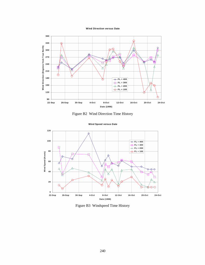
240

Wind Direction versus Date

90

120

150

180

210

240

270

300

330

360

22-Sep 26-Sep 30-Sep 4-Oct 8-O ct 12-Oct 16-Oct 20-O ct 24-Oct

Date (1998)

Win

d D

irec

tion

(D

egre

es f

rom

Tru

e N

ort

h)

FL = 400FL = 300

FL = 200FL = 100

Figure B2 Wind Direction Time History

Wind Speed versus Date

0

20

40

60

80

100

120

22-Sep 26-Sep 30-Sep 4-O ct 8-Oct 12-Oct 16-Oct 20-O ct 24-Oct

Date (1998)

Win

d S

pee

d (K

nots

)

FL = 400FL = 300FL = 200FL = 100

Figure B3 Windspeed Time History

241

APPENDIX C

AVERAGE SURFACE WEATHER FOR THE AIR FORCE FLIGHT TEST CENTER

242


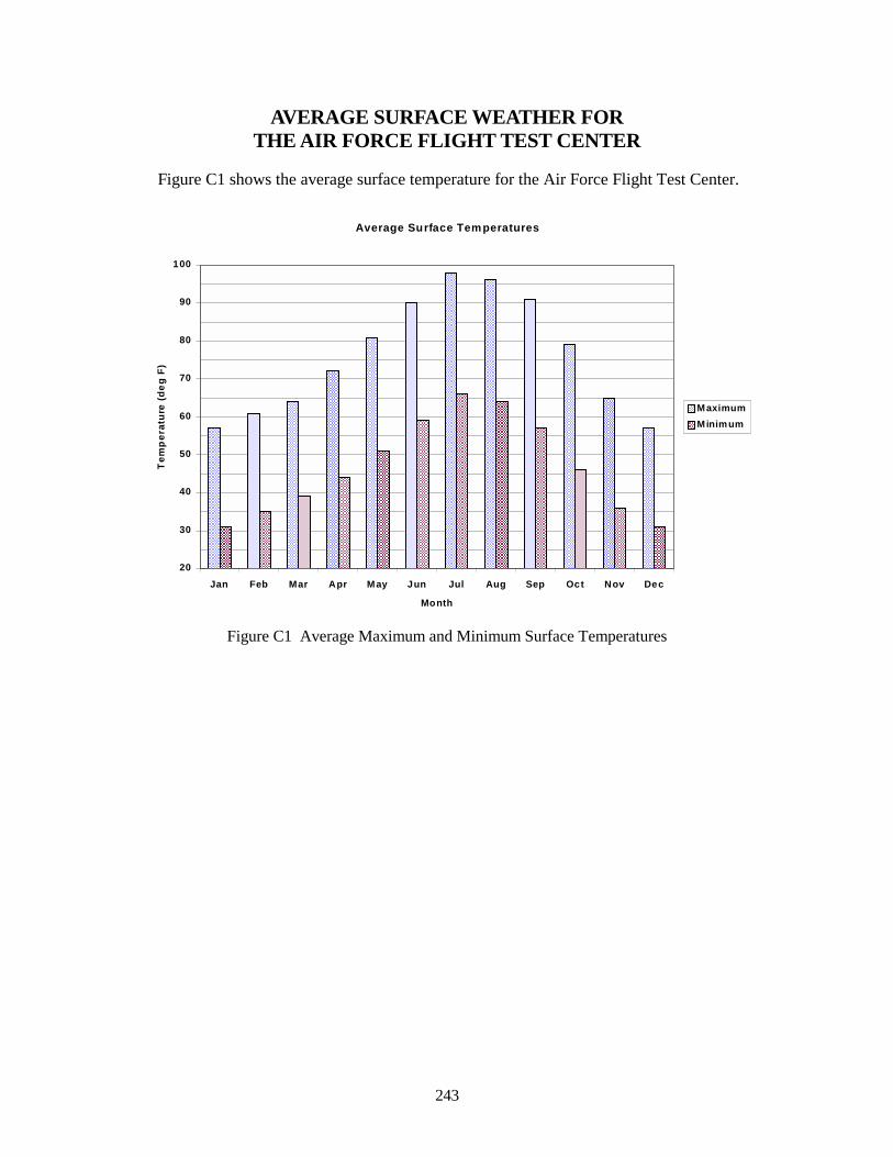
243

AVERAGE SURFACE WEATHER FOR THE AIR FORCE FLIGHT TEST CENTER

Figure C1 shows the average surface temperature for the Air Force Flight Test Center.

Average Surface Temperatures

20

30

40

50

60

70

80

90

100


Month

Tem

per

atur

e (d

eg F

)

MaximumMinimum

Figure C1 Average Maximum and Minimum Surface Temperatures

244


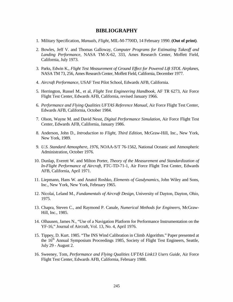
245

BIBLIOGRAPHY

1. Military Specification, Manuals, Flight, MIL-M-7700D, 14 February 1990. (Out of print).

2. Bowles, Jeff V. and Thomas Galloway, Computer Programs for Estimating Takeoff and Landing Performance, NASA TM-X-62, 333, Ames Research Center, Moffett Field, California, July 1973.

3. Parks, Edwin K., Flight Test Measurement of Ground Effect for Powered Lift STOL Airplanes, NASA TM 73, 256, Ames Research Center, Moffett Field, California, December 1977.

4. Aircraft Performance, USAF Test Pilot School, Edwards AFB, California.

5. Herrington, Russel M., et al, Flight Test Engineering Handbook, AF TR 6273, Air Force Flight Test Center, Edwards AFB, California, revised January 1966.

6. Performance and Flying Qualities UFTAS Reference Manual, Air Force Flight Test Center, Edwards AFB, California, October 1984.

7. Olson, Wayne M. and David Nesst, Digital Performance Simulation, Air Force Flight Test Center, Edwards AFB, California, January 1986.

8. Anderson, John D., Introduction to Flight, Third Edition, McGraw-Hill, Inc., New York, New York, 1989.

9. U.S. Standard Atmosphere, 1976, NOAA-S/T 76-1562, National Oceanic and Atmospheric Administration, October 1976.

10. Dunlap, Everett W. and Milton Porter, Theory of the Measurement and Standardization of In-Flight Performance of Aircraft, FTC-TD-71-1, Air Force Flight Test Center, Edwards AFB, California, April 1971.

11. Liepmann, Hans W. and Anatol Roshko, Elements of Gasdynamics, John Wiley and Sons, Inc., New York, New York, February 1965.

12. Nicolai, Leland M., Fundamentals of Aircraft Design, University of Dayton, Dayton, Ohio, 1975.

13. Chapra, Steven C., and Raymond P. Canale, Numerical Methods for Engineers, McGraw-Hill, Inc., 1985.

14. Olhausen, James N., “Use of a Navigation Platform for Performance Instrumentation on the YF-16,” Journal of Aircraft, Vol. 13, No. 4, April 1976.

15. Tippey, D. Kurt. 1985. “The INS Wind Calibration in Climb Algorithm.” Paper presented at the 16th Annual Symposium Proceedings 1985, Society of Flight Test Engineers, Seattle, July 29 - August 2.

16. Sweeney, Tom, Performance and Flying Qualities UFTAS Link13 Users Guide, Air Force Flight Test Center, Edwards AFB, California, February 1988.

246

BIBLIOGRAPHY (Continued)

17. Cheney, Harold. 1983. “Takeoff Performance Data Using Onboard Instrumentation.” Paper presented at the 14th Annual Symposium Proceedings, Society of Flight Test Engineers, Newport Beach, August 15-19.

18. GGD Publication 92-013, Geodesy and Geophysics Department, Defense Mapping Agency, Edwards AFB, California, July 1992.

19. Pope, Alan. April 1964. Wind Tunnel Testing, Second Edition, John Wiley and Sons, Inc.

20. Roskam, Jan, Flight Dynamics of Rigid and Elastic Airplanes, Roskam Aviation and Engineering Corporation, Lawrence, Kansas, 1976.

21. Etkin, Bernard. 1982. Dynamics of Flight, Second Edition. John Wiley and Sons.

22. Climatic Extremes for Military Equipment, MIL-STD-210A, U.S. Government Printing Office, August 1957. (Out of print).

23. DeAnda, Albert, AFFTC Standard Airspeed Calibration Procedures, Air Force Flight Test Center, Edwards AFB, California, June 1981.

24. Diehl, Walter, Engineering Aerodynamics, 1936.

25. Brown, W.G, “Measuring an Airplane’s True Speed in Flight Testing,” NACA Rep. TN 135, 1923.

26. Mair, W. Austyn, and David L. Birdsall, 1996. Aircraft Performance. Cambridge University Press.

27. Smith, H.C. 1992. The Illustrated Guide to Aerodynamics, Second Edition. Tab Books.

28. Wood, Karl D. 1955. Technical Aerodynamics, 3rd Edition. McGraw-Hill Book Company.

29. Collinson, R.P.G. 1997. Introduction to Avionics. Chapman & Hall.

30. Jones, Robert T. 1990. Wing Theory. Princeton University Press.

31. Fox, David. 1995. “Is Your Speed True.” KITPLANES Magazine (February).

32. Dwenger, Richard, Wheeler, John and James Lackey. 1997. “Use of GPS for an Altitude Reference Source for Air Data Testing.” Paper presented at the Society of Flight Test Engineers Symposium.

33. Kimberlin, Ralph and Joseph Sims. 1992. “Airspeed Calibration Using GPS.” AIAA 92-4090. Paper presented at the 6th Biennial Flight Test Conference, August 24-26.

34. http://www.navcen.uscg.mil/gps

35. Clark, Bill. 1994. Aviator’s Guide To GPS. TAB Books.

http://www.navcen.uscg.mil/gps

247

BIBLIOGRAPHY (Concluded)

36. NASA Allstar, www.allstar.fiu.edu/aero/research.htm

37. AIAA, www.aiaa.com

38. NASA Dryden, www.dfrc.nasa.gov

39. Denker, John S., See How It Fly’s, www.monmouth.com/~jsd/fly/how

40. Ojha, S.J., Flight Performance of Aircraft, AIAA Education Series, 1995.

41. Twaites, Bryan, ed. Incompressible Aerodynamics: An Account of the Steady Flow of Incompressible Fluid past Aerofoils, Wings and Other Bodies, Dover Publications.

42. Anderson, John D. 1998. A History of Aerodynamics. Cambridge University Press.

43. Chanute, Octave. 1897. Progress in Flying Machines. The American Engineer & Railroad Journal.

44. Lowry, John T., Performance of Light Aircraft, AIAA Education Series, 1999.

http://www.allstar.fiu.edu/aero/research.htm

http://www.aiaa.com/

http://www.dfrc.nasa.gov/

http://www.monmouth.com/~jsd/fly/how

248


249

LIST OF ABBREVIATIONS, ACRONYMS, AND SYMBOLS

Abbreviation Definition Unit

ADC air data computer ---

AF acceleration factor ---

AFB Air Force Base ---

AFFTC Air Force Flight Test Center ---

AGL above ground level ft

AIAA American Institute of Aeronautics and Astronautics ---

AOA angle of attack deg

AOSS angle of sideslip deg

A acceleration ft/sec²

AF acceleration factor ---

AR aspect ratio dimensionless

tAR aspect ratio of tanker dimensionless

DA acceleration in the down direction ft/sec2

EA acceleration in the east direction ft/sec2

NA acceleration in the north direction ft/sec2

bxA X axis body acceleration ft/sec2

byA Y-axis body acceleration ft/sec2

bzA Z-axis body acceleration ft/sec2

xA flight path longitudinal acceleration ft/sec2

xA longitudinal acceleration ft/sec²

yA flight path lateral acceleration ft/sec2

yA lateral acceleration ft/sec2

zA flight path normal acceleration ft/sec2

zA normal acceleration (positive down) ft/sec2

a acceleration ft/sec2

a speed of sound ktsNote: 1. Velocity units in knots or feet per second. 2. Time in units of seconds or hours.

250

LIST OF ABBREVIATIONS, ACRONYMS, AND SYMBOLS (Continued)


a temperature gradient °K/1,000 fta mean (average) acceleration ft/sec2

SLa speed of sound standard day sea level 1116.45 ft/sec; 661.48 kts

α angle of attack deg

/A Cα angle of attack from the aircraft system deg

INSα angle of attack computed from INS data deg

BAA body axis accelerometer ---

Btu British thermal unit ---

BHP brake horsepower HP

b wing span ft

C Celsius deg

DC drag coefficient dimensionless

minDC minimum drag coefficient ---

LC lift coefficient dimensionless

LbC break lift coefficient dimensionless

minLC lift coefficient at the minimum drag coefficient dimensionless

LtC tanker lift coefficient dimensionless

fcC compressible skin friction drag coefficient dimensionless

fiC incompressible skin friction drag coefficient dimensionless

cg center of gravity pct MAC

cg center of gravity pct MAC

cm centimeters ---

DGPS differential GPS ---

D down ---

D drag lbs

bwD drag of the aircraft body and wind lbs

251



sD standard day drag lbs

tD drag of the aircraft tail lbs

tD test day computed drag lbs

sD′ standard day predicted drag lbs

tD′ test day predicted drag lbs

d distance ft

tdV change in true airspeed ---

tdW weight increment lbs

dh change in altitude ft

dt time increment sec

dB decibels ---

deg degrees (either temperature or angle) ---

E east ---

EGI embedded GPS/INS ---

E east ---

E energy ft-lbs

F Fahrenheit deg

FL flight level (ft/100)

FPA flight path accelerometer ---

F Fahrenheit deg*F summation parameter to be minimized ---

eF propulsive drag lbs

exF excess thrust lbs

gF gross thrust lbs

nF net thrust lbs

nrF referred net thrust lbs

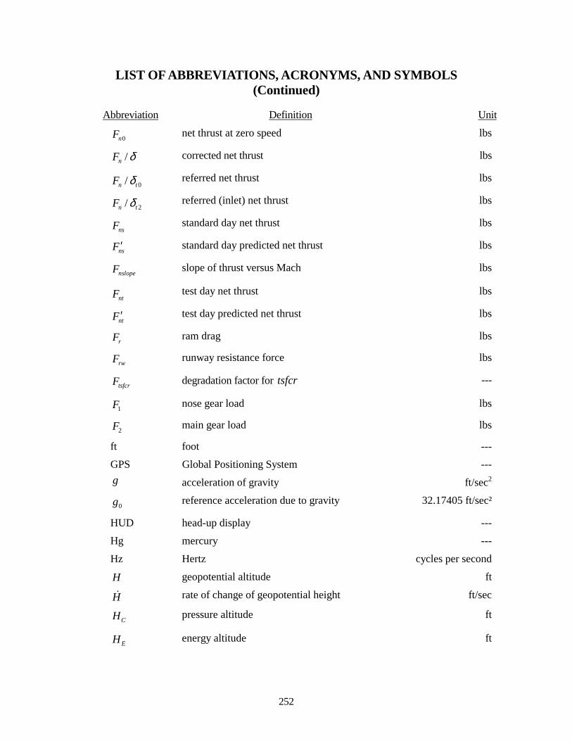
252



0nF net thrust at zero speed lbs

/nF δ corrected net thrust lbs

0/n tF δ referred net thrust lbs

2/n tF δ referred (inlet) net thrust lbs

nsF standard day net thrust lbs

nsF ′ standard day predicted net thrust lbs

nslopeF slope of thrust versus Mach lbs

ntF test day net thrust lbs

ntF ′ test day predicted net thrust lbs

rF ram drag lbs

rwF runway resistance force lbs

tsfcrF degradation factor for tsfcr ---

1F nose gear load lbs

2F main gear load lbs

ft foot ---

GPS Global Positioning System ---g acceleration of gravity ft/sec2

0g reference acceleration due to gravity 32.17405 ft/sec²

HUD head-up display ---

Hg mercury ---

Hz Hertz cycles per second

H geopotential altitude ft

H! rate of change of geopotential height ft/sec

CH pressure altitude ft

EH energy altitude ft

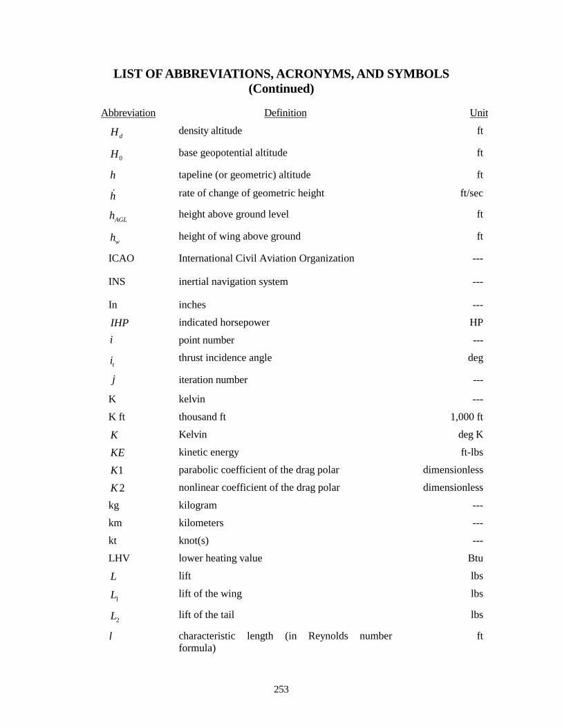
253



dH density altitude ft

0H base geopotential altitude ft

h tapeline (or geometric) altitude ft

h! rate of change of geometric height ft/sec

AGLh height above ground level ft

wh height of wing above ground ft

ICAO International Civil Aviation Organization ---

INS inertial navigation system ---

In inches ---

IHP indicated horsepower HPi point number ---

ti thrust incidence angle deg

j iteration number ---

K kelvin ---

K ft thousand ft 1,000 ft

K Kelvin deg K

KE kinetic energy ft-lbs

1K parabolic coefficient of the drag polar dimensionless

2K nonlinear coefficient of the drag polar dimensionless

kg kilogram ---

km kilometers ---

kt knot(s) ---

LHV lower heating value Btu

L lift lbs

1L lift of the wing lbs

2L lift of the tail lbs

l characteristic length (in Reynolds number formula)

ft

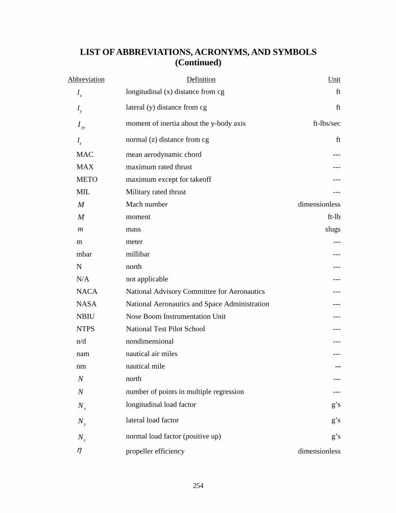
254



xl longitudinal (x) distance from cg ft

yl lateral (y) distance from cg ft

yyI moment of inertia about the y-body axis ft-lbs/sec

zl normal (z) distance from cg ft

MAC mean aerodynamic chord ---

MAX maximum rated thrust ---

METO maximum except for takeoff ---

MIL Military rated thrust ---

M Mach number dimensionless

M moment ft-lbm mass slugs

m meter ---

mbar millibar ---

N north ---

N/A not applicable ---

NACA National Advisory Committee for Aeronautics ---

NASA National Aeronautics and Space Administration ---

NBIU Nose Boom Instrumentation Unit ---

NTPS National Test Pilot School ---

n/d nondimensional ---

nam nautical air miles ---

nm nautical mile ---

N north ---

N number of points in multiple regression ---

xN longitudinal load factor g’s

yN lateral load factor g’s

zN normal load factor (positive up) g’s

η propeller efficiency dimensionless

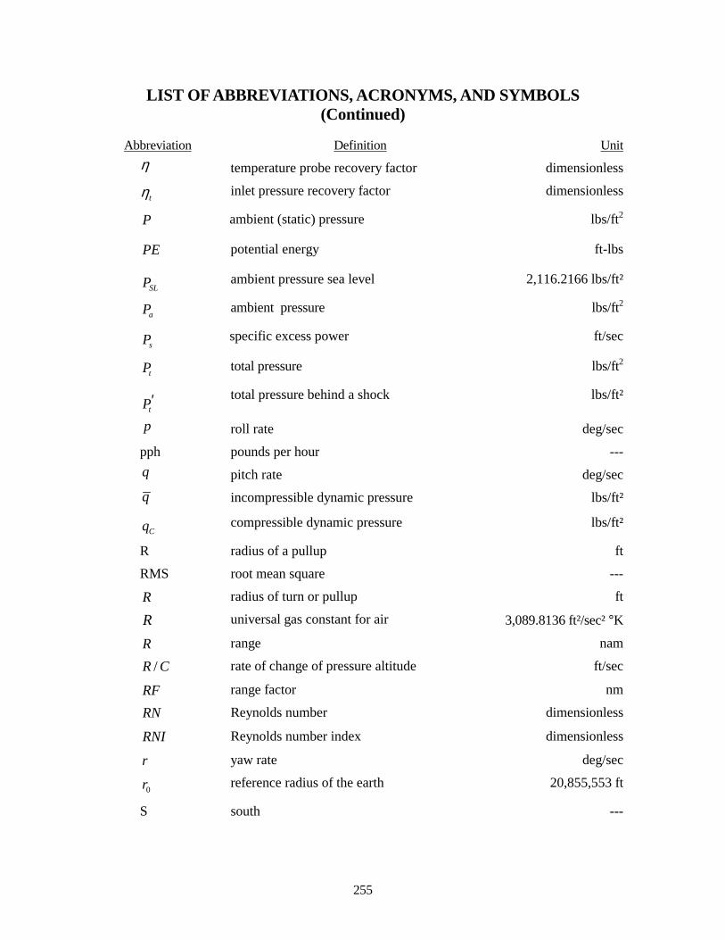
255


Abbreviation Definition Unitη temperature probe recovery factor dimensionless

tη inlet pressure recovery factor dimensionless

P ambient (static) pressure lbs/ft2

PE potential energy ft-lbs

SLP ambient pressure sea level 2,116.2166 lbs/ft²

aP ambient pressure lbs/ft2

sP specific excess power ft/sec

tP total pressure lbs/ft2

tP′ total pressure behind a shock lbs/ft²

p roll rate deg/sec

pph pounds per hour ---q pitch rate deg/secq incompressible dynamic pressure lbs/ft²

Cq compressible dynamic pressure lbs/ft²

R radius of a pullup ft

RMS root mean square ---

R radius of turn or pullup ft

R universal gas constant for air 3,089.8136 ft²/sec² °K

R range nam

/R C rate of change of pressure altitude ft/sec

RF range factor nm

RN Reynolds number dimensionless

RNI Reynolds number index dimensionless

r yaw rate deg/sec

0r reference radius of the earth 20,855,553 ft

S south ---

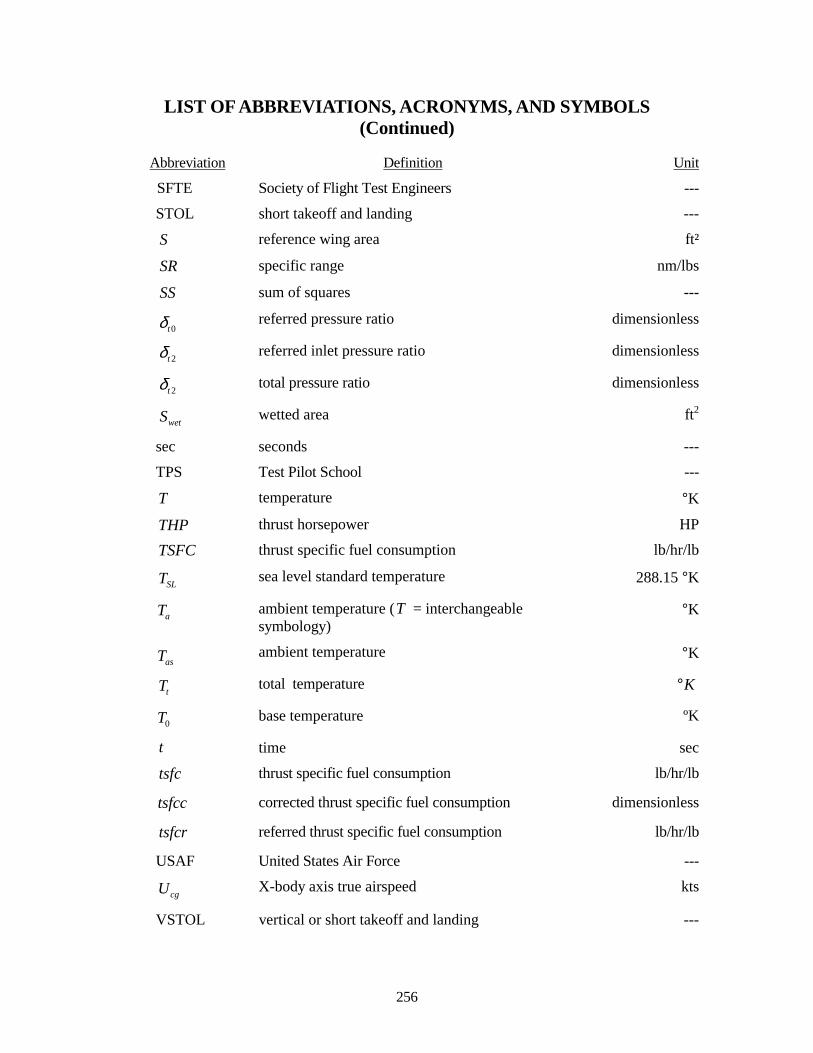
256



SFTE Society of Flight Test Engineers ---

STOL short takeoff and landing ---

S reference wing area ft²

SR specific range nm/lbs

SS sum of squares ---

0tδ referred pressure ratio dimensionless

2tδ referred inlet pressure ratio dimensionless

2tδ total pressure ratio dimensionless

wetS wetted area ft2

sec seconds ---

TPS Test Pilot School ---

T temperature °K

THP thrust horsepower HP

TSFC thrust specific fuel consumption lb/hr/lb

SLT sea level standard temperature 288.15 °K

aT ambient temperature (T = interchangeable symbology)

°K

asT ambient temperature °K

tT total temperature K°

0T base temperature ºK

t time sec

tsfc thrust specific fuel consumption lb/hr/lb

tsfcc corrected thrust specific fuel consumption dimensionless

tsfcr referred thrust specific fuel consumption lb/hr/lb

USAF United States Air Force ---

cgU X-body axis true airspeed kts

VSTOL vertical or short takeoff and landing ---

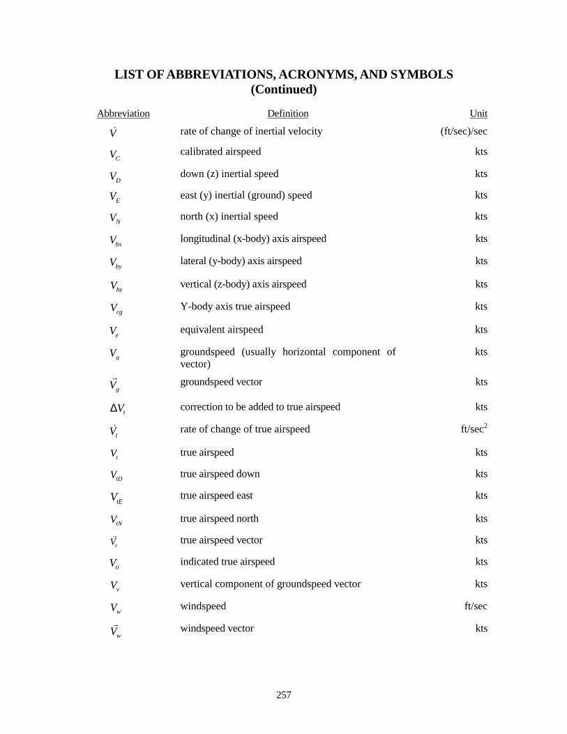
257



V! rate of change of inertial velocity (ft/sec)/sec

CV calibrated airspeed kts

DV down (z) inertial speed kts

EV east (y) inertial (ground) speed kts

NV north (x) inertial speed kts

bxV longitudinal (x-body) axis airspeed kts

byV lateral (y-body) axis airspeed kts

bzV vertical (z-body) axis airspeed kts

cgV Y-body axis true airspeed kts

eV equivalent airspeed kts

gV groundspeed (usually horizontal component of vector)

kts

gV"

groundspeed vector kts

tV∆ correction to be added to true airspeed kts

tV! rate of change of true airspeed ft/sec2

tV true airspeed kts

tDV true airspeed down kts

tEV true airspeed east kts

tNV true airspeed north kts

tV"

true airspeed vector kts

tiV indicated true airspeed kts

vV vertical component of groundspeed vector kts

wV windspeed ft/sec

wV"

windspeed vector kts

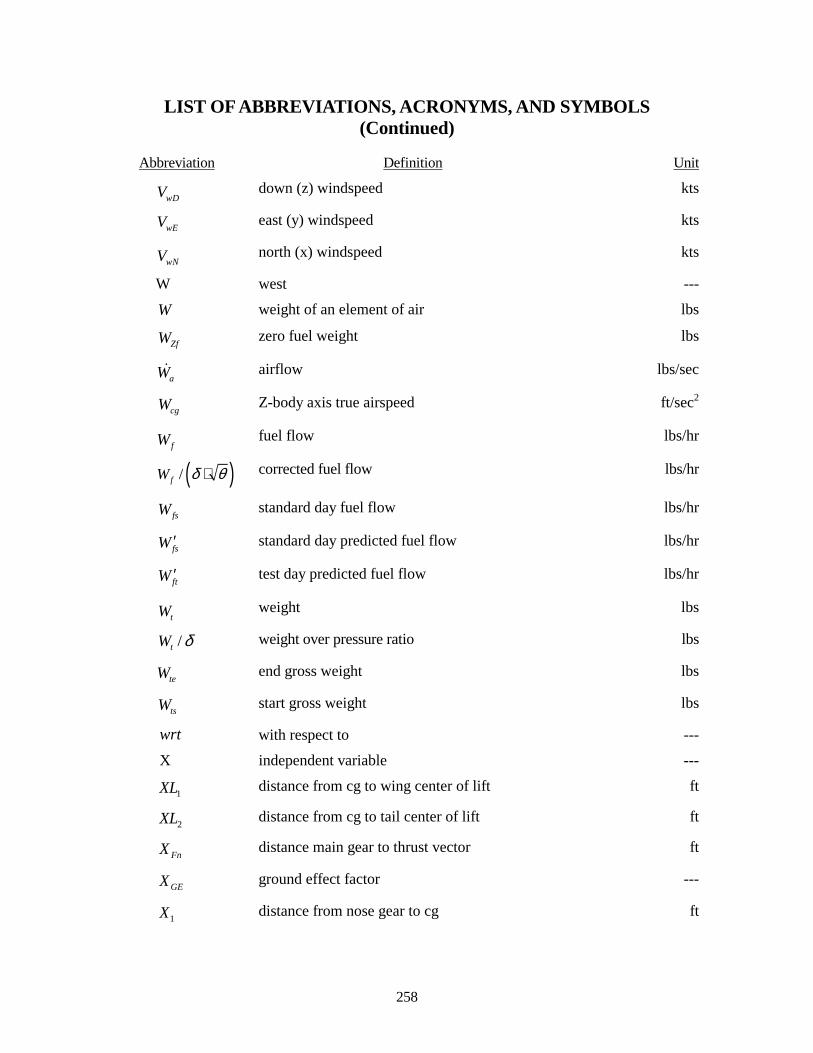
258



wDV down (z) windspeed kts

wEV east (y) windspeed kts

wNV north (x) windspeed kts

W west ---

W weight of an element of air lbs

ZfW zero fuel weight lbs

aW! airflow lbs/sec

cgW Z-body axis true airspeed ft/sec2

fW fuel flow lbs/hr

( )/fW δ θ⋅ corrected fuel flow lbs/hr

fsW standard day fuel flow lbs/hr

fsW ′ standard day predicted fuel flow lbs/hr

ftW ′ test day predicted fuel flow lbs/hr

tW weight lbs

/tW δ weight over pressure ratio lbs

teW end gross weight lbs

tsW start gross weight lbs

wrt with respect to ---

X independent variable ---

1XL distance from cg to wing center of lift ft

2XL distance from cg to tail center of lift ft

FnX distance main gear to thrust vector ft

GEX ground effect factor ---

1X distance from nose gear to cg ft

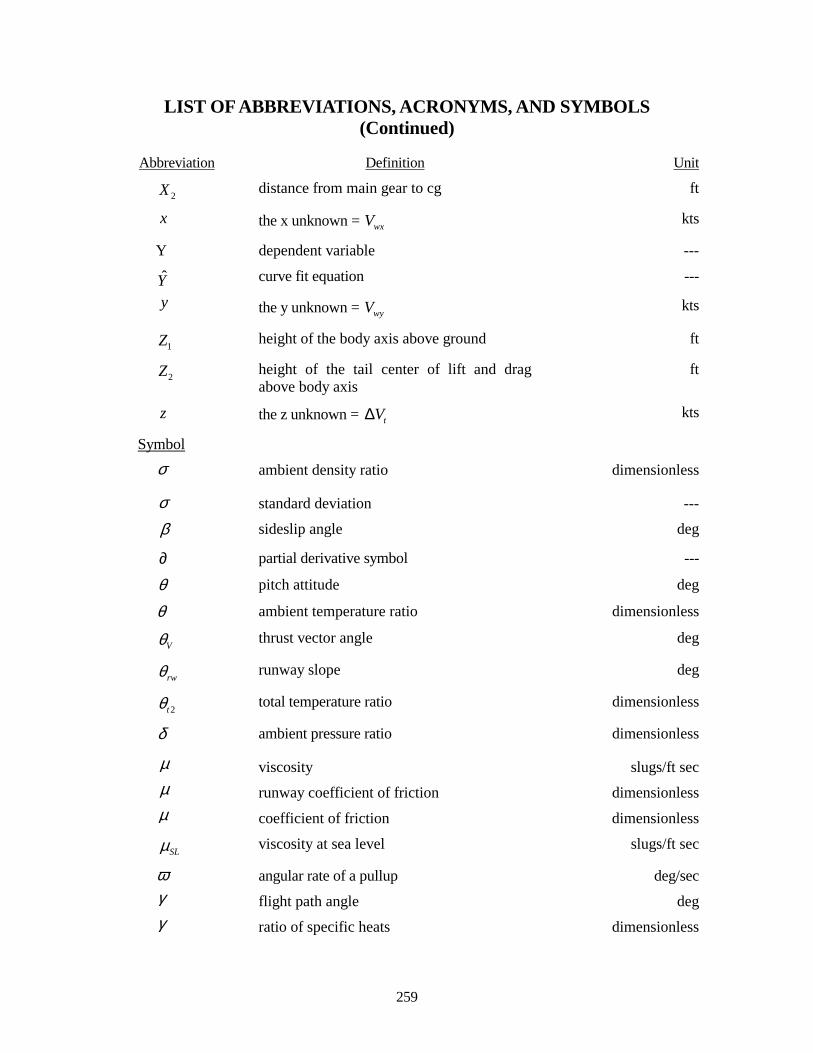
259



2X distance from main gear to cg ft

x the x unknown = wxV kts

Y dependent variable ---

Y curve fit equation ---

y the y unknown = wyV kts

1Z height of the body axis above ground ft

2Z height of the tail center of lift and drag above body axis

ft

z the z unknown = tV∆ kts

Symbol

σ ambient density ratio dimensionless

σ standard deviation ---

β sideslip angle deg

∂ partial derivative symbol ---

θ pitch attitude deg

θ ambient temperature ratio dimensionless

Vθ thrust vector angle deg

rwθ runway slope deg

2tθ total temperature ratio dimensionless

δ ambient pressure ratio dimensionless

µ viscosity slugs/ft secµ runway coefficient of friction dimensionlessµ coefficient of friction dimensionless

SLµ viscosity at sea level slugs/ft sec

ϖ angular rate of a pullup deg/secγ flight path angle degγ ratio of specific heats dimensionless

260

LIST OF ABBREVIATIONS, ACRONYMS, AND SYMBOLS (Concluded)

Symbol

0γ gravity at sea level (function of latitude) cm/sec2

φ bank angle deg

º degrees temperature or angle

λ engine losses factor ---ψ heading angle (degrees from true north) deg

∆ increment ---

∫ integral ---

ϕ latitude deg

φ roll attitude deg

∑ summation ---

0ε theoretical downwash angle deg

τ thrust increase time constant sec

gσ track angle deg from true north

261

INDEX

1976 U.S. Standard Atmosphere, 15, 16, 22, 31, 40, 174, 180

A Accelerating or decelerating turns, 155 acceleration, 1 Accelerometer

accelerometer noise, accelerometer rate corrections, 58, 60, 72

Aerobraking, 106, 112, 113 Airspeed, 12, 26, 30, 32, 35, 36, 37, 38, 83,

96, 100, 101, 104, 106, 111, 113, 116, 131, 134, 140, 150, 178, 246

Altitude Constant altitude, Energy altitude, 13, 15,

17, 18, 23, 24, 25, 26, 28, 42, 55, 114, 120, 121, 134, 136, 140, 141, 166, 170, 171, 178, 201, 202, 219, 236, 246, 251

Ambient pressure, 82 Angle of attack, 67 Atmosphere, 17, 23, 40, 245

B Braking

braking coefficient, braking forces, 3, 103, 106, 113

Butterworth filter Four-pole Butterworth filter, 61, 63

C Calibrated airspeed, 30, 83 Climb, 3, 144, 145, 146, 147, 149, 152, 181,

245 Cruise tests, 136

D Deceleration, 3, 104, 154, 181 Density, 13, 26 Density altitude, 13, 26 Descent, 3, 108, 154, 181 Differential GPS, 121 Differential pressure, 33 Drag, 2, 4, 40, 41, 43, 44, 45, 46, 80, 81, 97,

98, 108, 111, 112, 113, 165, 169, 184, 185, 186, 188, 189, 190, 191, 192, 206, 207

Drag coefficient, 81

Drag due to lift, 184 Dynamic performance, 164

E EGI, 114, 160, 179 Energy

kinetic energy, potential energy, 140 Equivalent airspeed, 37 Euler angles, 66, 73, 160 Excess thrust, 3, 57, 181, 182

F Fuel flow, 4, 180, 182

G Geometric altitude, 13 Geopotential altitude, 15 GPS, 2, 26, 30, 57, 58, 114, 115, 116, 122,

124, 125, 128, 129, 132, 134, 160, 218, 246, 250, 251

Gravity, 173 Groundspeed, 30, 129

I INS, 26, 30, 58, 66, 71, 112, 114, 135, 136,

144, 146, 154, 156, 158, 160, 168, 172, 176, 218, 245, 250, 251

Instrumentation, 1, 2, 60, 245, 246, 254

L Landing, 3, 75, 76, 103, 107, 109, 113, 245 Latitude, 174 Lift, 2, 4, 5, 40, 41, 44, 47, 82, 83, 84, 87, 94,

95, 97, 102, 108, 113, 189, 190 Lift coefficient, 82

M Mach number, 4, 30, 32, 33, 35, 39, 41, 42,

43, 45, 47, 52, 80, 81, 111, 116, 122, 126, 129, 135, 136, 140, 141, 142, 144, 145, 148, 151, 152, 155, 156, 164, 165, 167, 168, 172, 175, 177, 178, 184, 185, 186, 187, 188, 189, 191, 192, 194, 195, 197, 200, 202, 203, 206, 209, 217, 254

262

Maximum thrust, 54 Military thrust, 208 Minimum drag coefficient, 103

N NBIU (Nose Boom Instrumentation Unit), 59 Noise, 60 normal load factor, 152

P Pitot tube, 33 Pressure altitude, 21 Pressure ratio, 213 Pullup, 170, 171, 172

R Radar, 127, 134 Ram drag, 50 Range, 135, 136, 139, 140, 141, 142, 200,

201, 202, 203, 219 Range factor, 135, 140, 219 Range mission, 141 Rate corrections, 73 Refueling, 176 Reynolds number, 41, 42, 43, 80, 188, 194,

195, 199, 201, 202, 203, 213, 214, 215, 216, 217, 253, 255

Reynolds number index, 42, 194, 203, 216, 255

S Skin friction drag coefficient, 188 Split-S, 167, 169, 170, 172 Standard atmosphere, 85 Standard day, 25 Standardization, 180, 183, 245

T Takeoff, 3, 75, 76, 78, 86, 88, 97, 98, 99, 100,

101, 102, 113, 245, 246 Thrust, 2, 3, 6, 49, 50, 51, 53, 54, 81, 88, 92,

93, 102, 140, 145, 148, 193, 194, 195, 196, 197, 198, 204, 205, 206, 207, 208, 210, 211, 215, 218

Thrust runs, 81 Thrust specific fuel consumption, 193 Total pressure, 1

Total temperature, 1 True airspeed, 1, 30, 32, 125, 178 Turns, 155, 156

W Weather, 117, 237, 239, 241, 243 Windspeed, 25, 30, 236, 240

AIRCRAFT PERFORMANCE FLIGHT TESTING CHANGE FORM

Date: To: Frank Brown, 412 TW/TSFT Guide Revision No.: Page No.: Reads As: To Read: Reason for Recommended Change: Organization: Name and Grade/Organization: Signature:

264

FROM: Frank Brown 412 TW/TSFT 195 E. Popson Ave. Edwards AFB, California 93524-6841

Aircraft Performance Flight Testing

Documents

Transcript of Aircraft Performance Flight Testing