Airborne Topographic Mapper Calibration Procedures and ... · Airborne Topographic Mapper...

Airborne Topographic Mapper Calibration Procedures and Accuracy Assessment

NASA/TM–2012-215891

February 2012

Chreston F. Martin, WIlliam B. Krabill, Serdar S. Manizade, Rob L. Russell, John G. Sonntag, Robert N. Swift, and James K. Yungel

National Aeronautics and Space Administration

Goddard Space Flight Center Greenbelt, Maryland 20771

https://ntrs.nasa.gov/search.jsp?R=20120008479 2019-02-02T23:07:29+00:00Z

Since its founding, NASA has been dedicated to the advancement of aeronautics and space science. The NASA scientific and technical information (STI) pro-gram plays a key part in helping NASA maintain this important role.

The NASA STI program operates under the auspices of the Agency Chief Information Officer. It collects, organizes, provides for archiving, and disseminates NASA’s STI. The NASA STI program provides access to the NASA Aeronautics and Space Database and its public interface, the NASA Technical Report Server, thus providing one of the largest collections of aero-nautical and space science STI in the world. Results are published in both non-NASA channels and by NASA in the NASA STI Report Series, which includes the following report types:

• TECHNICAL PUBLICATION. Reports of completed research or a major significant phase of research that present the results of NASA Programs and include extensive data or theoretical analysis. Includes compilations of significant scientific and technical data and information deemed to be of continuing reference value. NASA counterpart of peer-reviewed formal professional papers but has less stringent limitations on manuscript length and extent of graphic presentations.

• TECHNICAL MEMORANDUM. Scientific and technical findings that are preliminary or of specialized interest, e.g., quick release reports, working papers, and bibliographies that contain minimal annotation. Does not contain extensive analysis.

• CONTRACTOR REPORT. Scientific and technical findings by NASA-sponsored contractors and grantees.

• CONFERENCE PUBLICATION. Collected papers from scientific and technical conferences, symposia, seminars, or other meetings sponsored or co-sponsored by NASA.

• SPECIAL PUBLICATION. Scientific, technical, or historical information from NASA programs, projects, and missions, often concerned with subjects having substantial public interest.

• TECHNICAL TRANSLATION. English-language translations of foreign scientific and technical material pertinent to NASA’s mission.

Specialized services also include organizing and publishing research results, distributing specialized research announcements and feeds, providing help desk and personal search support, and enabling data exchange services. For more information about the NASA STI program, see the following:

• Access the NASA STI program home page at http://www.sti.nasa.gov

• E-mail your question via the Internet to [email protected]

• Fax your question to the NASA STI Help Desk at 443-757-5803

• Phone the NASA STI Help Desk at 443-757-5802

• Write to:

NASA STI Help Desk NASA Center for AeroSpace Information 7115 Standard Drive Hanover, MD 21076-1320

NASA STI Program ... in Profile

National Aeronautics and Space Administration

Goddard Space Flight Center Greenbelt, Maryland 20771


NASA/TM–2012-215891

February 2012

Chreston F. Martin Sigma Space, Inc., Lanham, MD William B. Krabill Sigma Space, Inc., Lanham, MD Serdar S. Manizade URS, Inc., San Francisco, CA Rob L. Russell Sigma Space, Inc., Lanham, MD John G. Sonntag URS, Inc., San Francisco, CA Robert N. Swift Sigma Space, Inc., Lanham, MD James K. Yungel URS, Inc., San Francisco, CA

Available from: NASA Center for AeroSpace Information 7115 Standard Drive Hanover, MD 21076-1320

National Technical Information Service 5285 Port Royal Road Springfield, VA 22161 Price Code: A17

Level of Review: This material has been technically reviewed by technical management

Trade names and trademarks are used in this report for identification only. Their usage does not constitute an official endorsement, either expressed or implied, by the National Aeronautics and Space Administration.

Notice for Copyrighted Information

This manuscript has been authored by employees of Sigma Space Inc. named under Contract No. NNG09HP18C with the National Aeronautics and Space Administration. The United States Government has a nonexclusive, irrevocable, worldwide license to prepare derivative works, publish, or reproduce this manuscript, and allow others to do so, for United States Government purposes. Any publisher accepting this manuscript for publication acknowledges that the United States Government retains such a license in any published form of this manuscript. All other rights are retained by the copyright owner.

i

Table of Contents Table of Contents ...................................................................................................................................... iv List of Tables ............................................................................................................................................... iv List of Figures .............................................................................................................................................. v 1.0 Introduction .......................................................................................................................................... 1 2.0 ATM System Description ................................................................................................................. 4 3.0 ATM Calibration and Accuracy Assessment ........................................................................... 7 3.1 ATM Calibration from Ramp Pass Overflights .................................................................. 7 3.2 Crossing Pass Accuracy Assessment ................................................................................... 10

4.0 Trajectory Computation and Accuracy ................................................................................... 15 5.0 Attitude Errors and Their Effects on Surveys ...................................................................... 22 6.0 Error in Knowledge of Horizontal Footprint Positioning ............................................... 26 6.1 Laser Pulse Timing Errors ....................................................................................................... 27 6.2 Scan and Date Timing Errors ................................................................................................. 27 6.3 Scan Azimuth Bias Error .......................................................................................................... 28 6.4 Heading Bias Error ..................................................................................................................... 28 6.5 Pitch and Roll Error .................................................................................................................... 29 6.6 Heading Error ............................................................................................................................... 29 6.7 GPS Positioning Error ................................................................................................................ 29 6.8 Total Horizontal Error .............................................................................................................. 30

7.0 Error Analysis Summary ............................................................................................................... 30 8.0 References ........................................................................................................................................... 32

List of Tables Table 1. Parameter Estimates from Punta Arenas Ramp Passes from Fall 2009 .......... 7 Table 2. Measured Range Calibration for ATM T3 Laser .......................................................... 8 Table 3. Estimated Range Biases from Ramp Passes. α Fixed at 11.062°. ........................ 9 Table 4. Summary of Crossover Differences from ATM Campaigns. ................................. 21 Table 5. Summary of Estimated Pitch and Roll Errors for ATM Missions. ...................... 26 Table 6. Summary of Estimated Pitch and Roll Errors for ATM Missions (converted into vertical error). ................................................................................................................................. 26 Table 7. Characteristics and Accuracies of ATM Ice Sheet Surveys. .................................. 31

ii

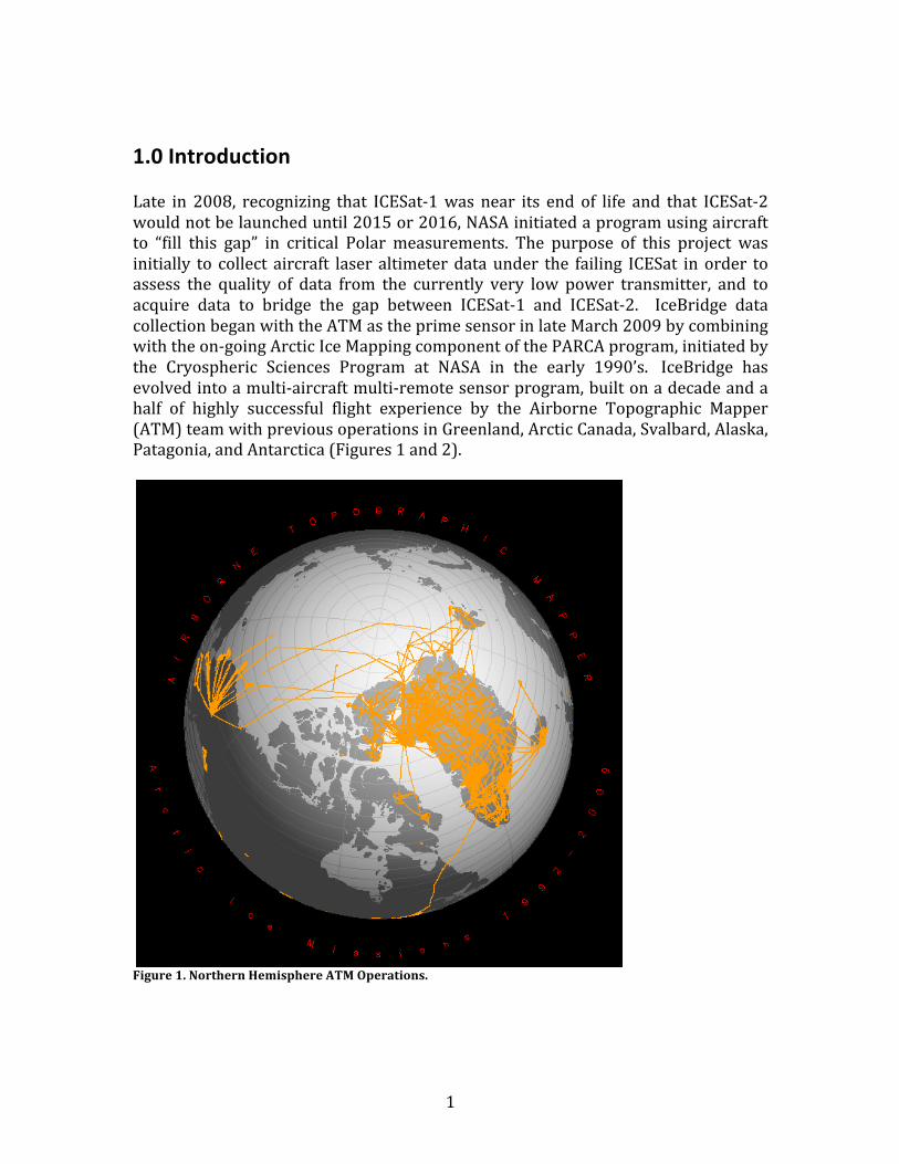
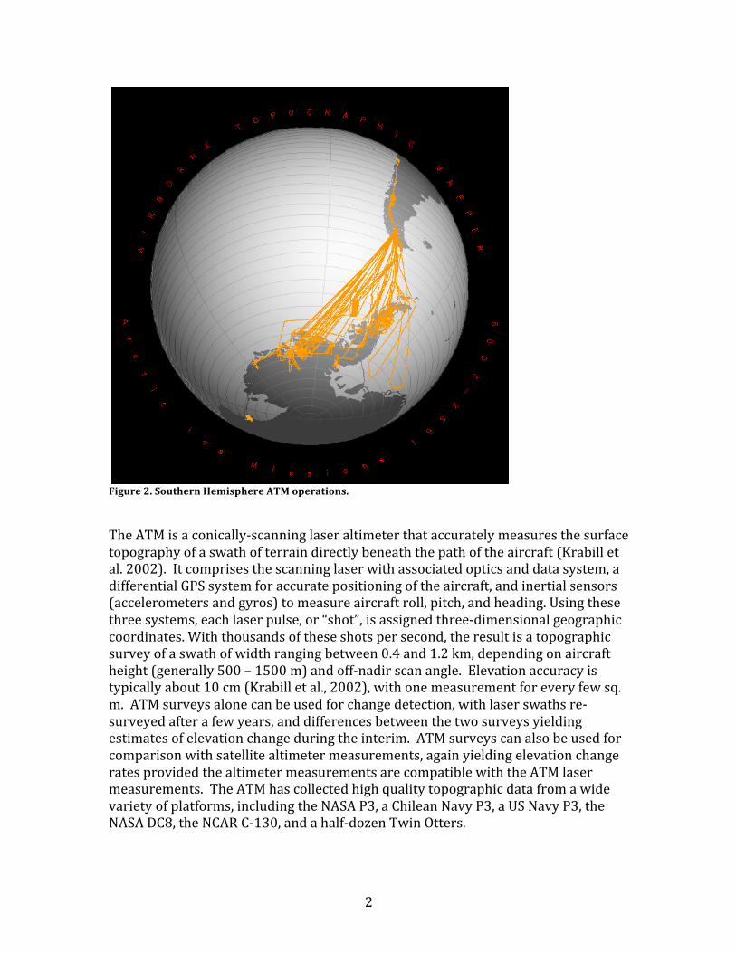
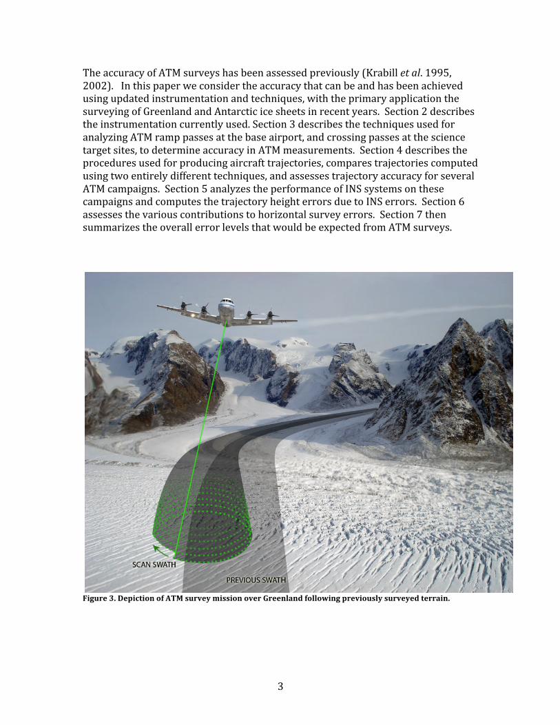
List of Figures Figure 1. Northern Hemisphere ATM Operations. ...................................................................... 1 Figure 2. Southern Hemisphere ATM operations. ....................................................................... 2 Figure 3. Depiction of ATM survey mission over Greenland following previously surveyed terrain. ........................................................................................................................................ 3 Figure 4. Primary instrumentation components of the Airborne Topographic Mapper. .......................................................................................................................................................... 4 Figure 5. Aircraft layout of ATM components. Measurements of dX, dY (not shown) and dZ=dZ1+dZ2 are made with tape measure and plumb bob. ............................................ 6 Figure 6. Devicq Glacier ATM crossing. .......................................................................................... 11 Figure 7. Crossing pass ATM elevations. ....................................................................................... 12 Figure 8. Estimated corrections for crossing point elevation differences. ..................... 14 Figure 9. Computed corrections for crossing pass along latitude band -‐74.92625°. . 14 Figure 10. Groundtracks for 2009 Antarctica campaign. ....................................................... 17 Figure 11. Groundtracks for 2010 Greenland campaigns. ..................................................... 18 Figure 12. Mean and RMS differences between Applanix and gitar trajectory heights for 2009 Antarctica campaign. ........................................................................................................... 19 Figure 13. Mean and RMS differences between Applanix and gitar trajectory heights for 2010 Greenland DC8 campaign. ................................................................................................. 20 Figure 14. Pitch and roll errors estimated for the 2008 DC8 deployment to Antarctica. ................................................................................................................................................... 23 Figure 15. Pitch and roll errors estimated for the 2010 DC8 deployment to Greenland. ................................................................................................................................................... 24 Figure 16. Pitch and roll errors estimated for the 2010 P3 deployment to Greenland. ......................................................................................................................................................................... 25

1

1.0 Introduction Late in 2008, recognizing that ICESat-‐1 was near its end of life and that ICESat-‐2 would not be launched until 2015 or 2016, NASA initiated a program using aircraft to “fill this gap” in critical Polar measurements. The purpose of this project was initially to collect aircraft laser altimeter data under the failing ICESat in order to assess the quality of data from the currently very low power transmitter, and to acquire data to bridge the gap between ICESat-‐1 and ICESat-‐2. IceBridge data collection began with the ATM as the prime sensor in late March 2009 by combining with the on-‐going Arctic Ice Mapping component of the PARCA program, initiated by the Cryospheric Sciences Program at NASA in the early 1990’s. IceBridge has evolved into a multi-‐aircraft multi-‐remote sensor program, built on a decade and a half of highly successful flight experience by the Airborne Topographic Mapper (ATM) team with previous operations in Greenland, Arctic Canada, Svalbard, Alaska, Patagonia, and Antarctica (Figures 1 and 2).

Figure 1. Northern Hemisphere ATM Operations.

2

Figure 2. Southern Hemisphere ATM operations.

The ATM is a conically-‐scanning laser altimeter that accurately measures the surface topography of a swath of terrain directly beneath the path of the aircraft (Krabill et al. 2002). It comprises the scanning laser with associated optics and data system, a differential GPS system for accurate positioning of the aircraft, and inertial sensors (accelerometers and gyros) to measure aircraft roll, pitch, and heading. Using these three systems, each laser pulse, or “shot”, is assigned three-‐dimensional geographic coordinates. With thousands of these shots per second, the result is a topographic survey of a swath of width ranging between 0.4 and 1.2 km, depending on aircraft height (generally 500 – 1500 m) and off-‐nadir scan angle. Elevation accuracy is typically about 10 cm (Krabill et al., 2002), with one measurement for every few sq. m. ATM surveys alone can be used for change detection, with laser swaths re-‐surveyed after a few years, and differences between the two surveys yielding estimates of elevation change during the interim. ATM surveys can also be used for comparison with satellite altimeter measurements, again yielding elevation change rates provided the altimeter measurements are compatible with the ATM laser measurements. The ATM has collected high quality topographic data from a wide variety of platforms, including the NASA P3, a Chilean Navy P3, a US Navy P3, the NASA DC8, the NCAR C-‐130, and a half-‐dozen Twin Otters.

3

The accuracy of ATM surveys has been assessed previously (Krabill et al. 1995, 2002). In this paper we consider the accuracy that can be and has been achieved using updated instrumentation and techniques, with the primary application the surveying of Greenland and Antarctic ice sheets in recent years. Section 2 describes the instrumentation currently used. Section 3 describes the techniques used for analyzing ATM ramp passes at the base airport, and crossing passes at the science target sites, to determine accuracy in ATM measurements. Section 4 describes the procedures used for producing aircraft trajectories, compares trajectories computed using two entirely different techniques, and assesses trajectory accuracy for several ATM campaigns. Section 5 analyzes the performance of INS systems on these campaigns and computes the trajectory height errors due to INS errors. Section 6 assesses the various contributions to horizontal survey errors. Section 7 then summarizes the overall error levels that would be expected from ATM surveys.

Figure 3. Depiction of ATM survey mission over Greenland following previously surveyed terrain.

4

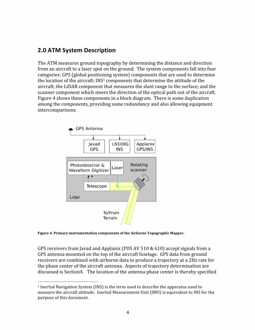
2.0 ATM System Description The ATM measures ground topography by determining the distance and direction from an aircraft to a laser spot on the ground. The system components fall into four categories: GPS (global positioning system) components that are used to determine the location of the aircraft; INS1 components that determine the attitude of the aircraft; the LiDAR component that measures the slant range to the surface; and the scanner component which steers the direction of the optical path out of the aircraft. Figure 4 shows these components in a block diagram. There is some duplication among the components, providing some redundancy and also allowing equipment intercomparisons.

Figure 4. Primary instrumentation components of the Airborne Topographic Mapper.

GPS receivers from Javad and Applanix (POS AV 510 & 610) accept signals from a GPS antenna mounted on the top of the aircraft fuselage. GPS data from ground receivers are combined with airborne data to produce a trajectory at a 2Hz rate for the phase center of the aircraft antenna. Aspects of trajectory determination are discussed is Section4. The location of the antenna phase center is thereby specified

1 Inertial Navigation System (INS) is the term used to describe the apparatus used to measure the aircraft attitude. Inertial Measurement Unit (IMU) is equivalent to INS for the purpose of this document.

5

in the most recent ITRF, i.e. the Terrestrial Reference Frame defined by the International Earth Rotation and Reference Systems Service. Attitude is provided by the Applanix units and by a Litton LN-‐100G INS/GPS. Specifically, these units measure the heading, pitch, and roll angles of the units themselves, which may differ slightly from the aircraft frame or from the ATM frame. The primary (and most accurate) INS measurement is the Applanix Model 610 system. Factory specifications for the 610 are (http://www.applanix.com/media/downloads/products/specs/POSAV_SPECS.pdf, version issued June 2009):

Applanix GPS trajectory accuracy: POS AV Absolute Accuracy (RMS) Model 610 Post Processed Position: 0.05 to 0.30 meters Applanix POS AV INS POS AV Absolute Accuracy (RMS) Model 610 Post Processed Roll and Pitch 0.0025° True Heading 0.0050°

In order to meet the attitude specifications, the aircraft must make 180° maneuvers periodically, so the numbers are somewhat optimistic for realistic mapping missions. A detailed discussion related to aircraft attitude determination and correction is presented in Section 5. The LiDAR contains a pulsed green laser that is directed downward from the aircraft, nominally at a 5 kHz rate. A telescope coaligned with the laser receives the signal backscattered from the ground below, and, if the input signal exceeds a set threshold, sends it through a photodetector to an Acqiris 8 bit waveform digitizer that captures typically 160 samples at 0.5 nsec resolution. A portion of the transmitted laser pulse is also sent to the photodetector and digitizer via an optical fiber. The delay between laser pulse transmission and the detection of the reflection from the ice surface is extracted from the digitized waveforms during post flight processing. Applying a 75% constant-‐fraction leading edge tracking algorithm to both transmit and receive pulses with an empirically derived adjustment for saturated waveforms refines the elapsed time between the two waveforms. The time delay multiplied by the speed of light through the atmosphere yields slant range. Accuracy of correlating transmitted and received pulses is around 0.2 nsec, leading to a noise floor of around 3 cm in range. Atmospheric refraction correction is applied to the range at a later stage of processing with consideration of the aircraft altitude and a quadratic model of refraction versus altitude. The scanner is a mirror rotating about an axis which is slightly offset from the mirror normal. The scanner typically rotates at 20 Hz. The instantaneous position, called the scan azimuth, is determined from a pulse generated once per revolution. The high frequency errors in azimuth measurement will be discussed in Section 6 and the azimuth bias error will be discussed in Section 3.1.

6

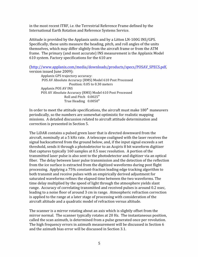
Two ATM systems have operated on most Operation IceBridge missions, each scanner having a different scan angle (maximum off-‐nadir angle). For several years, scanners having a 22° and 15° angle have been operated, and a 2.5° scanner was flown during the spring 2009 campaign. At a nominal altitude of 500m above ground level, the 22° scanner sweeps the LiDAR footprint across a 400m wide swath. The scanners typically spin at a 20 Hz rate. In the following sections, the LiDAR transceiver with the 22° scanner may be referred to as the T3 laser and the 15° one as the T2 laser. The geometric relationship of the ATM components on the aircraft is shown in Figure 5. The separation between the GPS antenna and the scan mirror on an aircraft can be as much as 4 m horizontally and 4 m vertically. Transforming coordinates from the GPS to the scan mirror relies in part on tape measure and plumb bob measurements (as shown in the Figure 5) which are measured once (in aircraft coordinates) and then assumed constant for a campaign. In addition, measurements by the attitude sensor are needed to account for changing aircraft orientation. Other parameters needed to convert laser ranges to surface coordinates (latitude, longitude, and elevation) are the orientation (heading, pitch, and roll) of the scan mirror and the two angles, α and β, shown in Figure 5. The estimation of these parameters, their errors, and their effects will be discussed in Section 3.1.

Figure 5. Aircraft layout of ATM components. Measurements of dX, dY (not shown) and dZ=dZ1+dZ2 are made with tape measure and plumb bob.

7

3.0 ATM Calibration and Accuracy Assessment The ATM system, as discussed in the previous section, includes a number of components and also requires the calibration of a number of parameters. This calibration is normally performed around a base site which includes a ground GPS receiver and a surveyed surface against which to compare the ATM ranging measurements. The surveyed surface is usually a ramp surface at an airbase. For assessment of performance during a mission, crossings of mission flight paths are the primary tools for measuring consistency and inferring accuracy. Ramp passes and crossing passes are discussed separately below.

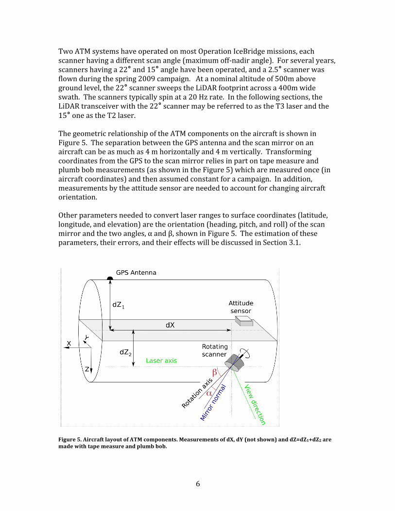
3.1 ATM Calibration from Ramp Pass Overflights The ATM (along with associated inertial measuring instruments) is almost always installed on the aircraft a few days or weeks prior to a campaign and is then rather promptly uninstalled after the campaign. In order to obtain the desired survey accuracy, the ATM must be appropriately aligned with the INS system. We refer to the ATM mounting angles relative to the INS orientation as heading, pitch, and roll mounting biases. In addition to these three mounting angles, there are several other angles associated with the scanning laser system: the angle beta (β shown in Figure3) between the entering laser beam and the spin axis of the scan mirror; the angle alpha (α shown in Figure 3) between the scan mirror spin axis and the normal to the scan mirror; and the bias in the measured azimuth of the scan. To one degree or another, all these parameters can be estimated from passes over surveyed airport ramps. Table 1. Parameter Estimates from Punta Arenas Ramp Passes from Fall 2009

Parameter Name Parameter Value

Change Sigma

Scan Azimuth Bias 1 257.445508 0.008008 0.026952 Alpha 11.063178 -0.000922 0.004842 Beta 44.503711 -0.023689 0.031430 INS Lag -0.007712 -0.007712 0.005469 Scanner Head Bias 179.644490 -0.250610 0.107223 Scanner Pitch Bias -0.401050 0.005950 0.004028 Scanner Roll Bias -0.068854 0.011046 0.030808 Scanner Range Bias -25.940646 -0.015646 0.027136

The basic geometry of a ramp pass is similar to that shown in Figure 1 except that the surface underneath the aircraft is not ice but rather a surveyed ramp. The ATM provides measurements of range and scan angle; the INS provides heading, pitch, and roll; and the GPS (aircraft and ground) receivers provide position of the aircraft GPS receiver. From these measurements, the above six biases need to be estimated. Table 1 shows the summary of the results of processing eight ramp passes from the

8

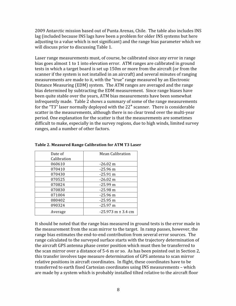
2009 Antarctic mission based out of Punta Arenas, Chile. The table also includes INS lag (included because INS lags have been a problem for older INS systems but here adjusting to a value which is not significant) and the range bias parameter which we will discuss prior to discussing Table 1. Laser range measurements must, of course, be calibrated since any error in range bias goes almost 1 to 1 into elevation error. ATM ranges are calibrated in ground tests in which a target board is set up 150m or more from the aircraft (or from the scanner if the system is not installed in an aircraft) and several minutes of ranging measurements are made to it, with the “true” range measured by an Electronic Distance Measuring (EDM) system. The ATM ranges are averaged and the range bias determined by subtracting the EDM measurement. Since range biases have been quite stable over the years, ATM bias measurements have been somewhat infrequently made. Table 2 shows a summary of some of the range measurements for the “T3” laser normally deployed with the 22° scanner. There is considerable scatter in the measurements, although there is no clear trend over the multi-‐year period. One explanation for the scatter is that the measurements are sometimes difficult to make, especially in the survey regions, due to high winds, limited survey ranges, and a number of other factors. Table 2. Measured Range Calibration for ATM T3 Laser

Date of Calibration

Mean Calibration

060610 -‐26.02 m 070410 -‐25.96 m 070430 -‐25.91 m 070525 -‐26.02 m 070824 -‐25.99 m 070830 -‐25.98 m 071004 -‐25.96 m 080402 -‐25.95 m 090324 -‐25.97 m Average -‐25.973 m ± 3.4 cm

It should be noted that the range bias measured in ground tests is the error made in the measurement from the scan mirror to the target. In ramp passes, however, the range bias estimates the end-‐to-‐end contribution from several error sources. The range calculated to the surveyed surface starts with the trajectory determination of the aircraft GPS antenna phase center position which must then be transferred to the scan mirror over a distance of 5-‐6 m or so. As has been pointed out in Section 2, this transfer involves tape measure determination of GPS antenna to scan mirror relative positions in aircraft coordinates. In flight, these coordinates have to be transferred to earth fixed Cartesian coordinates using INS measurements – which are made by a system which is probably installed tilted relative to the aircraft floor

9

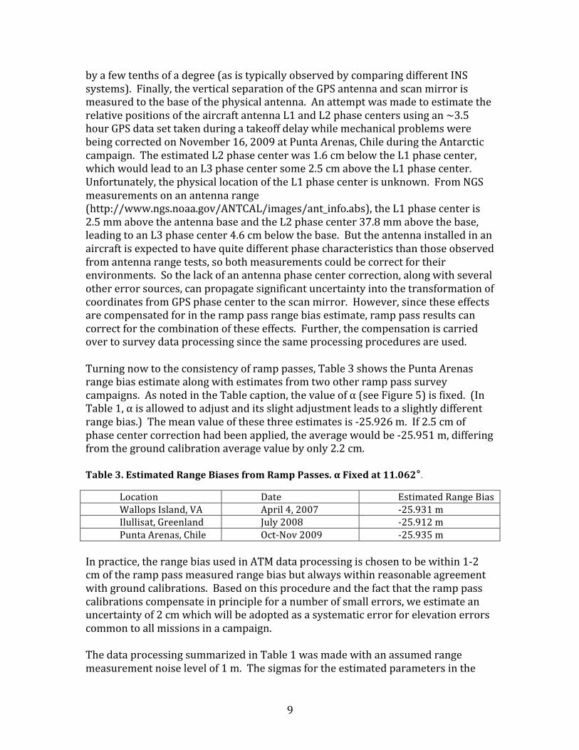
by a few tenths of a degree (as is typically observed by comparing different INS systems). Finally, the vertical separation of the GPS antenna and scan mirror is measured to the base of the physical antenna. An attempt was made to estimate the relative positions of the aircraft antenna L1 and L2 phase centers using an ~3.5 hour GPS data set taken during a takeoff delay while mechanical problems were being corrected on November 16, 2009 at Punta Arenas, Chile during the Antarctic campaign. The estimated L2 phase center was 1.6 cm below the L1 phase center, which would lead to an L3 phase center some 2.5 cm above the L1 phase center. Unfortunately, the physical location of the L1 phase center is unknown. From NGS measurements on an antenna range (http://www.ngs.noaa.gov/ANTCAL/images/ant_info.abs), the L1 phase center is 2.5 mm above the antenna base and the L2 phase center 37.8 mm above the base, leading to an L3 phase center 4.6 cm below the base. But the antenna installed in an aircraft is expected to have quite different phase characteristics than those observed from antenna range tests, so both measurements could be correct for their environments. So the lack of an antenna phase center correction, along with several other error sources, can propagate significant uncertainty into the transformation of coordinates from GPS phase center to the scan mirror. However, since these effects are compensated for in the ramp pass range bias estimate, ramp pass results can correct for the combination of these effects. Further, the compensation is carried over to survey data processing since the same processing procedures are used. Turning now to the consistency of ramp passes, Table 3 shows the Punta Arenas range bias estimate along with estimates from two other ramp pass survey campaigns. As noted in the Table caption, the value of α (see Figure 5) is fixed. (In Table 1, α is allowed to adjust and its slight adjustment leads to a slightly different range bias.) The mean value of these three estimates is -‐25.926 m. If 2.5 cm of phase center correction had been applied, the average would be -‐25.951 m, differing from the ground calibration average value by only 2.2 cm. Table 3. Estimated Range Biases from Ramp Passes. α Fixed at 11.062°.

Location Date Estimated Range Bias Wallops Island, VA April 4, 2007 -‐25.931 m Ilullisat, Greenland July 2008 -‐25.912 m Punta Arenas, Chile Oct-‐Nov 2009 -‐25.935 m

In practice, the range bias used in ATM data processing is chosen to be within 1-‐2 cm of the ramp pass measured range bias but always within reasonable agreement with ground calibrations. Based on this procedure and the fact that the ramp pass calibrations compensate in principle for a number of small errors, we estimate an uncertainty of 2 cm which will be adopted as a systematic error for elevation errors common to all missions in a campaign. The data processing summarized in Table 1 was made with an assumed range measurement noise level of 1 m. The sigmas for the estimated parameters in the

10

table (units for range are meters and degrees for angles) should thus be conservative considering that the RMS data fits are better than 10 cm. The parameter with the largest uncertainty is scanner heading bias, but the estimate should still be better than 0.1°. Sigmas for beta and roll mounting bias look much larger than the sigma for pitch bias. However, the correlation between the two is very high (0.988) so the combined effect on a scan position should be comparable to that for pitch. The correlation between alpha and range bias (0.85) also looks high. For a single pass, the correlation would be near 1.0 because the aircraft determines the height, which is related to range and α by the approximate relation Height ≈ Range * cos(2α) (1) With multiple passes at different heights over the ramps, the correlation becomes sufficiently small that both range bias and α can be estimated with reasonable confidence.

3.2 Crossing Pass Accuracy Assessment While nominal values of parameters affecting ATM survey accuracy are determined from passes over surveyed ramp surfaces normally at the aircraft base station and close to a ground GPS site used as a reference for the aircraft trajectory, performance at the primary survey site hundreds of kilometers away can be quite different. The INS system used can be expected to drift to some extent and aircraft trajectory accuracy will be affected by the large separation from the ground base station (or stations). For these reasons, attempts are made to validate system parameters at the survey site to the extent possible. The primary technique used for this validation is the use of crossing ATM passes, either on the same mission day or on different days. Such passes normally occur simply due to the nature of the survey mission, with a prime example being detailed glacier surveys in which aircraft tracks are performed in a grid pattern. The assumption made in processing crossing passes is that the surface topography remains unchanged between the passes. The validity of this assumption varies, of course, with the dynamics of the surveyed terrain and decreases with time. However, we would expect crossing passes made on the same day to find very similar topography and passes separated by a few days do have a high probability of similar topography except at very low elevations. Assuming similar topography, the primary parameters which would be expected to affect the differences in topography measured by two crossing passes are aircraft pitch and roll errors and trajectory height errors (more specifically, differences between the trajectory height errors). For same day crossings, the height error differences would be expected to be rather small since a high proportion of the systematic errors in the trajectories should be common. In general, height differences for passes separated by only by a day or two would be expected to be

11

Assuming similar topography, the primary parameters which would be expected to affect the differences in topography measured by two crossing passes are aircraft pitch and roll errors and trajectory height errors (more specifically, differences between the trajectory height errors). For same day crossings, the height error differences would be expected to be rather small since a high proportion of the systematic errors in the trajectories should be common. In general, height differences for passes separated by only by a day or two would be expected to be larger than same-‐day crossing differences, primarily due to systematic trajectory errors, although this depends upon topography variability. It should also be noted that there is a limit to how rough the terrain can be without having so much noise that little can be extracted from the pass differences.

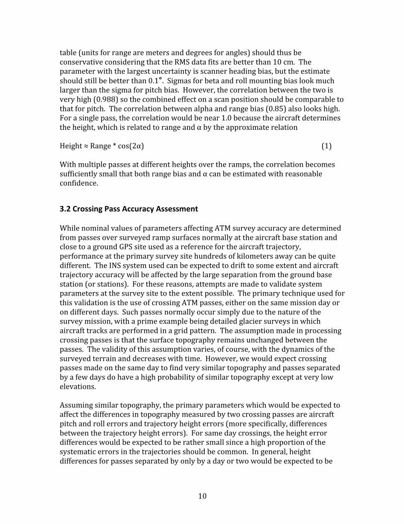
Figure 6. Devicq Glacier ATM crossing.

Figure 6 shows the location of two ATM crossing passes made on October 16, 2009 on Devicq glacier in Antarctica. The circled crossing will be discussed here. As will be noted from the figure, the two passes cross at a near 90° angle, a desirable characteristic for accurate parameter estimation. Figure 7 shows the spots whose locations and elevations were measured by each pass. The points are color-‐coded to show the elevations (around 250m) along the two swaths and are separated by only about 30 minutes in time. It will be noted that the edges of the earlier pass (the vertical one) is slightly curved, indicating that the aircraft is in a slight turn, consistent with the track shown in Figure 6. The procedure used in processing the crossing is to difference the elevation of each point in the later pass from the elevation of points in the earlier pass that are within a specified distance (2 m nominally). This gives a residual and there are typically some 10000 or more residuals in a crossover. An estimation is then made of the elevation difference and

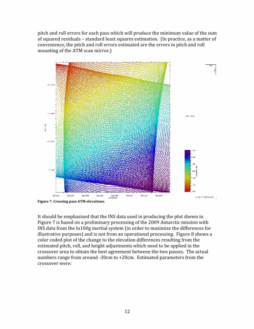
12

pitch and roll errors for each pass which will produce the minimum value of the sum of squared residuals – standard least squares estimation. (In practice, as a matter of convenience, the pitch and roll errors estimated are the errors in pitch and roll mounting of the ATM scan mirror.)

Figure 7. Crossing pass ATM elevations.

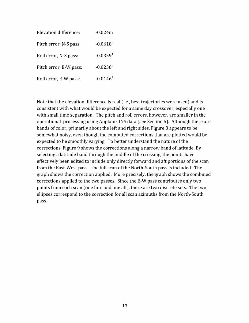
It should be emphasized that the INS data used in producing the plot shown in Figure 7 is based on a preliminary processing of the 2009 Antarctic mission with INS data from the ln100g inertial system (in order to maximize the differences for illustrative purposes) and is not from an operational processing. Figure 8 shows a color coded plot of the change to the elevation differences resulting from the estimated pitch, roll, and height adjustments which need to be applied in the crossover area to obtain the best agreement between the two passes. The actual numbers range from around -‐30cm to +20cm. Estimated parameters from the crossover were:

13

Elevation difference: -‐0.024m

Pitch error, N-‐S pass: -‐0.0618°

Roll error, N-‐S pass: -‐0.0359°

Pitch error, E-‐W pass: -‐0.0238°

Roll error, E-‐W pass: -‐0.0146°

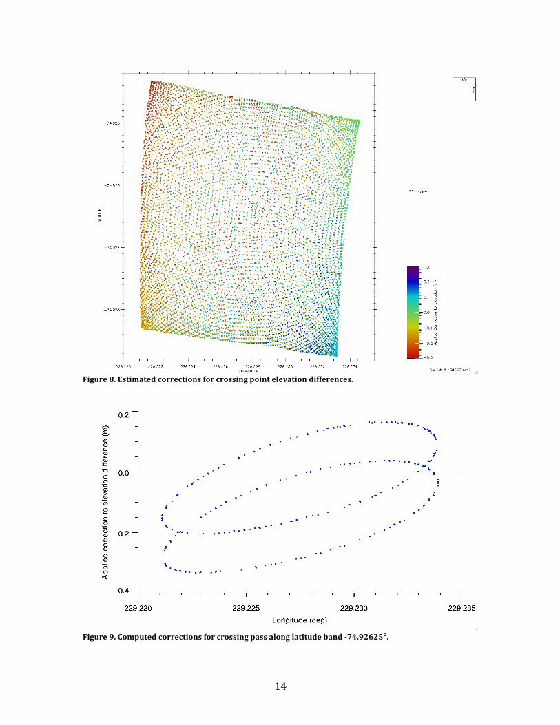
Note that the elevation difference is real (i.e., best trajectories were used) and is consistent with what would be expected for a same day crossover, especially one with small time separation. The pitch and roll errors, however, are smaller in the operational processing using Applanix INS data (see Section 5). Although there are bands of color, primarily about the left and right sides, Figure 8 appears to be somewhat noisy, even though the computed corrections that are plotted would be expected to be smoothly varying. To better understand the nature of the corrections, Figure 9 shows the corrections along a narrow band of latitude. By selecting a latitude band through the middle of the crossing, the points have effectively been edited to include only directly forward and aft portions of the scan from the East-‐West pass. The full scan of the North-‐South pass is included. The graph shows the correction applied. More precisely, the graph shows the combined corrections applied to the two passes. Since the E-‐W pass contributes only two points from each scan (one fore and one aft), there are two discrete sets. The two ellipses correspond to the correction for all scan azimuths from the North-‐South pass.

14

Figure 8. Estimated corrections for crossing point elevation differences.

Figure 9. Computed corrections for crossing pass along latitude band -‐74.92625°.

15

Although elevation differences estimated from crossing passes near sea level do not represent trajectory error but rather geophysical effects such as tide changes, such crossings can still produce good estimates of pitch and roll errors from reasonably smooth surfaces. It should be noted that if pitch and roll errors are not of particular concern, the above technique can be used to estimate elevation changes at any elevation regardless of surface roughness. In fact, the program in which the technique is implemented (“altdify”) was specifically developed for doing elevation difference computations over rough surfaces. In addition, it was primarily intended to difference alongtrack passes.

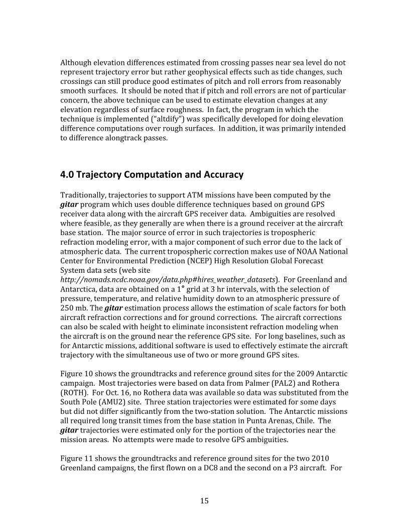
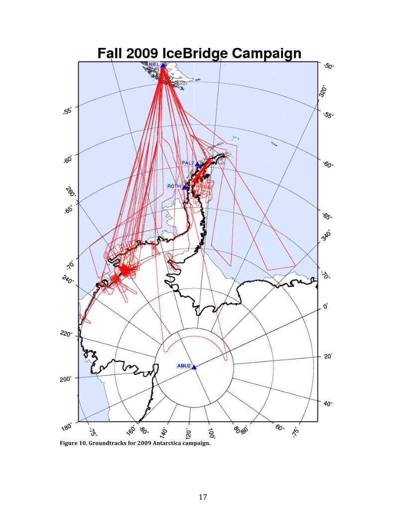
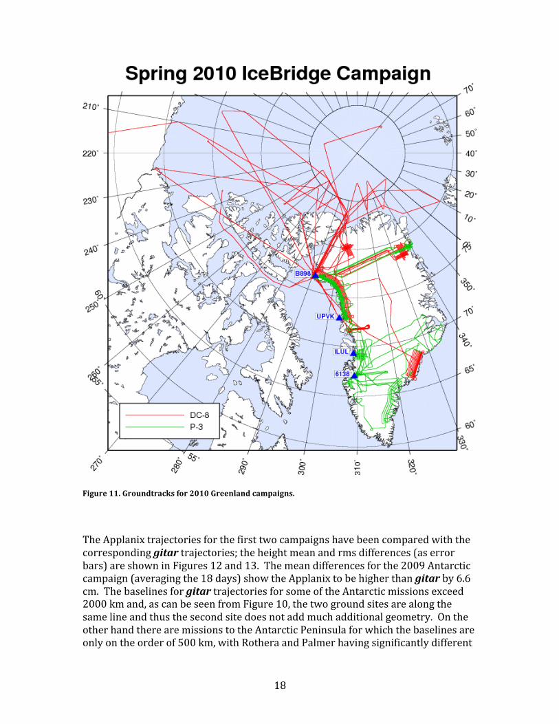
4.0 Trajectory Computation and Accuracy Traditionally, trajectories to support ATM missions have been computed by the gitar program which uses double difference techniques based on ground GPS receiver data along with the aircraft GPS receiver data. Ambiguities are resolved where feasible, as they generally are when there is a ground receiver at the aircraft base station. The major source of error in such trajectories is tropospheric refraction modeling error, with a major component of such error due to the lack of atmospheric data. The current tropospheric correction makes use of NOAA National Center for Environmental Prediction (NCEP) High Resolution Global Forecast System data sets (web site http://nomads.ncdc.noaa.gov/data.php#hires_weather_datasets). For Greenland and Antarctica, data are obtained on a 1° grid at 3 hr intervals, with the selection of pressure, temperature, and relative humidity down to an atmospheric pressure of 250 mb. The gitar estimation process allows the estimation of scale factors for both aircraft refraction corrections and for ground corrections. The aircraft corrections can also be scaled with height to eliminate inconsistent refraction modeling when the aircraft is on the ground near the reference GPS site. For long baselines, such as for Antarctic missions, additional software is used to effectively estimate the aircraft trajectory with the simultaneous use of two or more ground GPS sites. Figure 10 shows the groundtracks and reference ground sites for the 2009 Antarctic campaign. Most trajectories were based on data from Palmer (PAL2) and Rothera (ROTH). For Oct. 16, no Rothera data was available so data was substituted from the South Pole (AMU2) site. Three station trajectories were estimated for some days but did not differ significantly from the two-‐station solution. The Antarctic missions all required long transit times from the base station in Punta Arenas, Chile. The gitar trajectories were estimated only for the portion of the trajectories near the mission areas. No attempts were made to resolve GPS ambiguities. Figure 11 shows the groundtracks and reference ground sites for the two 2010 Greenland campaigns, the first flown on a DC8 and the second on a P3 aircraft. For

16

the DC8 campaign, all missions were based out of Thule (B898) and only single-‐station trajectories were estimated. For the P3 campaign, flights were flown out of Kangerlussuaq (6138) prior to April 17. On April 17, the aircraft transited to Thule and subsequent missions were flown out of Thule. Single station trajectories were estimated using the base station GPS except for the transit mission. For the transit mission, data was available and used from Ilulissat (ILUL) and Upernavik (UPVK) , with no base station data available. With the recent introduction of the Applanix systems, primarily for improvements in INS accuracy, an additional procedure for computing aircraft trajectories is available. Using Applanix post-‐mission processing software (plus various data sets), trajectories can be computed without the use of any ground sites (a mode exists also to use ground sites, but this mode has not been extensively exercised). For recent ATM campaigns, trajectories have been computed using the Applanix software and data from an Applanix 510 system for the 2009 Antarctic campaign, an Applanix 610 system for the 2010 Greenland campaign, and an Applanix 510 system for the 2010 Greenland P3 campaign (610 data is also available for a portion of the P3 campaign). The stated accuracy of the Applanix trajectories (see Section 2) is 5-‐30 cm, a rather wide range. The conditions are not clearly defined as to when a 5 cm accuracy can be expected and when a 30 cm accuracy is to be expected. So we have compared available Applanix trajectories with gitar trajectories to see how they compare for different regions, baseline lengths and trajectory lengths. If the trajectories are found to be robust (not susceptible to gross errors) and to have accuracies comparable to those using gitar we may adopt the procedure.

17

Figure 10. Groundtracks for 2009 Antarctica campaign.

18

Figure 11. Groundtracks for 2010 Greenland campaigns.

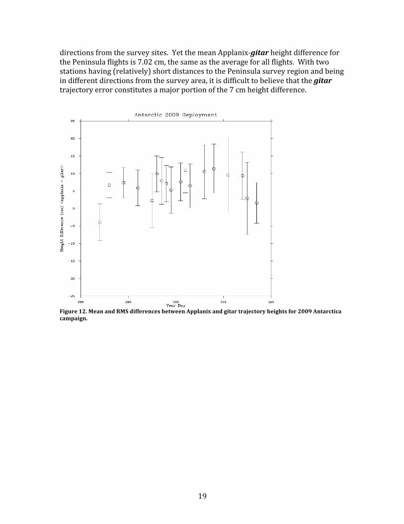
The Applanix trajectories for the first two campaigns have been compared with the corresponding gitar trajectories; the height mean and rms differences (as error bars) are shown in Figures 12 and 13. The mean differences for the 2009 Antarctic campaign (averaging the 18 days) show the Applanix to be higher than gitar by 6.6 cm. The baselines for gitar trajectories for some of the Antarctic missions exceed 2000 km and, as can be seen from Figure 10, the two ground sites are along the same line and thus the second site does not add much additional geometry. On the other hand there are missions to the Antarctic Peninsula for which the baselines are only on the order of 500 km, with Rothera and Palmer having significantly different

19

directions from the survey sites. Yet the mean Applanix-‐gitar height difference for the Peninsula flights is 7.02 cm, the same as the average for all flights. With two stations having (relatively) short distances to the Peninsula survey region and being in different directions from the survey area, it is difficult to believe that the gitar trajectory error constitutes a major portion of the 7 cm height difference.

Figure 12. Mean and RMS differences between Applanix and gitar trajectory heights for 2009 Antarctica campaign.

20

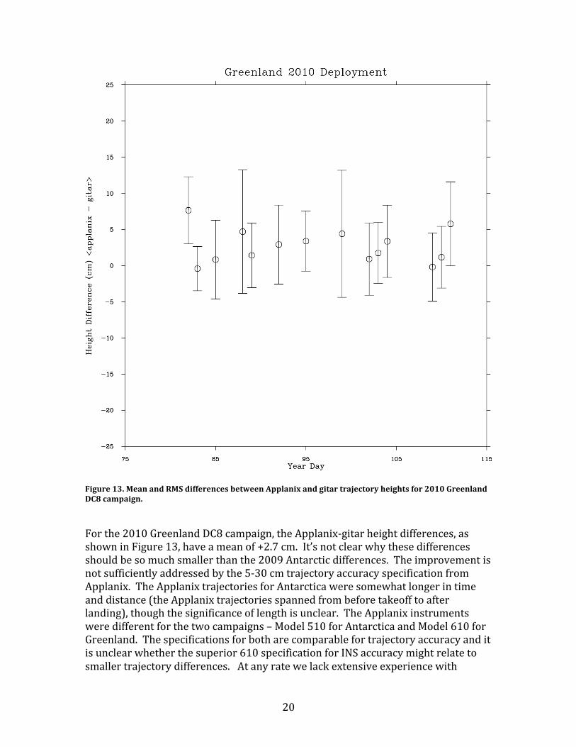
Figure 13. Mean and RMS differences between Applanix and gitar trajectory heights for 2010 Greenland DC8 campaign.

For the 2010 Greenland DC8 campaign, the Applanix-‐gitar height differences, as shown in Figure 13, have a mean of +2.7 cm. It’s not clear why these differences should be so much smaller than the 2009 Antarctic differences. The improvement is not sufficiently addressed by the 5-‐30 cm trajectory accuracy specification from Applanix. The Applanix trajectories for Antarctica were somewhat longer in time and distance (the Applanix trajectories spanned from before takeoff to after landing), though the significance of length is unclear. The Applanix instruments were different for the two campaigns – Model 510 for Antarctica and Model 610 for Greenland. The specifications for both are comparable for trajectory accuracy and it is unclear whether the superior 610 specification for INS accuracy might relate to smaller trajectory differences. At any rate we lack extensive experience with

21

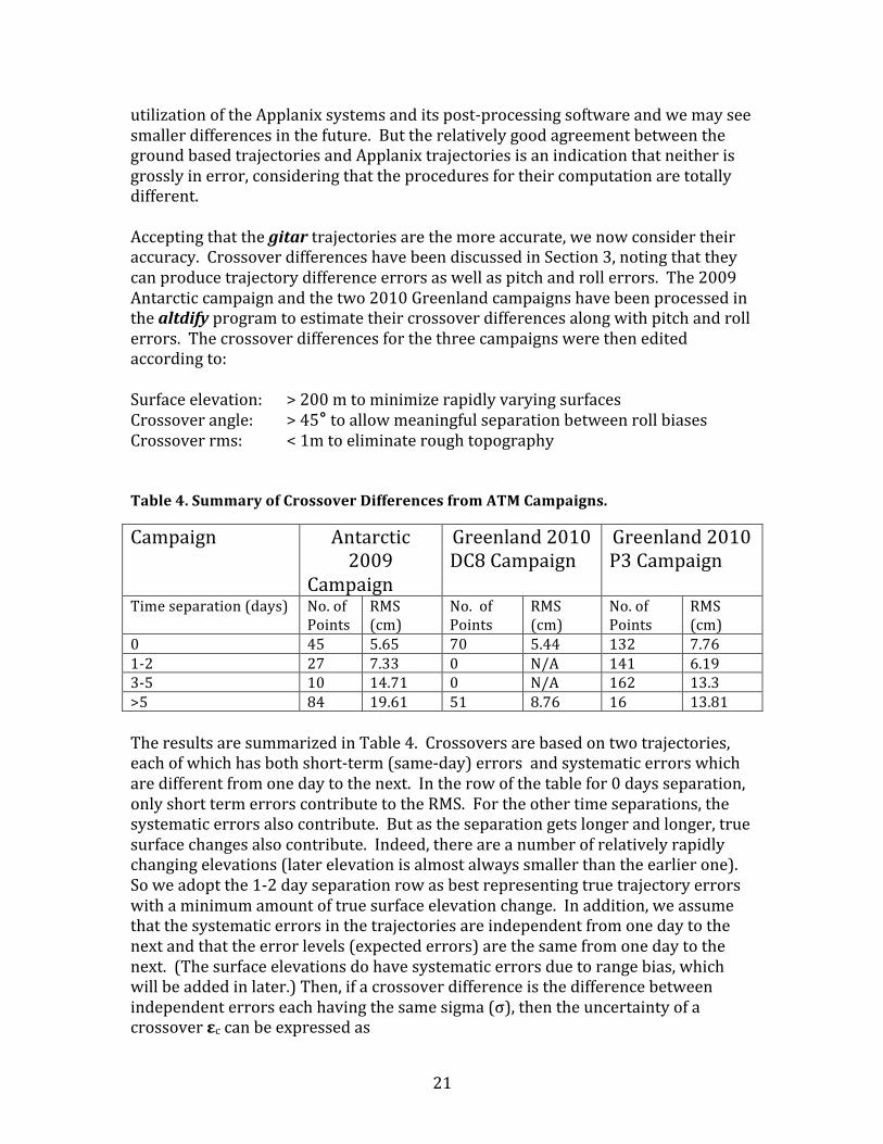
utilization of the Applanix systems and its post-‐processing software and we may see smaller differences in the future. But the relatively good agreement between the ground based trajectories and Applanix trajectories is an indication that neither is grossly in error, considering that the procedures for their computation are totally different. Accepting that the gitar trajectories are the more accurate, we now consider their accuracy. Crossover differences have been discussed in Section 3, noting that they can produce trajectory difference errors as well as pitch and roll errors. The 2009 Antarctic campaign and the two 2010 Greenland campaigns have been processed in the altdify program to estimate their crossover differences along with pitch and roll errors. The crossover differences for the three campaigns were then edited according to: Surface elevation: > 200 m to minimize rapidly varying surfaces Crossover angle: > 45° to allow meaningful separation between roll biases Crossover rms: < 1m to eliminate rough topography Table 4. Summary of Crossover Differences from ATM Campaigns.

Campaign Antarctic 2009

Campaign

Greenland 2010 DC8 Campaign

Greenland 2010 P3 Campaign

Time separation (days) No. of Points

RMS (cm)

No. of Points

RMS (cm)

No. of Points

RMS (cm)

0 45 5.65 70 5.44 132 7.76 1-‐2 27 7.33 0 N/A 141 6.19 3-‐5 10 14.71 0 N/A 162 13.3 >5 84 19.61 51 8.76 16 13.81 The results are summarized in Table 4. Crossovers are based on two trajectories, each of which has both short-‐term (same-‐day) errors and systematic errors which are different from one day to the next. In the row of the table for 0 days separation, only short term errors contribute to the RMS. For the other time separations, the systematic errors also contribute. But as the separation gets longer and longer, true surface changes also contribute. Indeed, there are a number of relatively rapidly changing elevations (later elevation is almost always smaller than the earlier one). So we adopt the 1-‐2 day separation row as best representing true trajectory errors with a minimum amount of true surface elevation change. In addition, we assume that the systematic errors in the trajectories are independent from one day to the next and that the error levels (expected errors) are the same from one day to the next. (The surface elevations do have systematic errors due to range bias, which will be added in later.) Then, if a crossover difference is the difference between independent errors each having the same sigma (σ), then the uncertainty of a crossover εc can be expressed as

22

εc = ε2 -‐ ε1 (2) which says only that the crossover error is the difference of the errors from each pass. But, given the independence of the errors from one pass from another, the expected value of the square of the crossover error is E(εc)2 = E(ε2)2 +2E(ε1 ε2) + E(ε1)2 = 2 σ2 (3) Since the errors are independent from one day to the next and the expected error for each day is the same. It follows that the individual pass trajectory uncertainty is σ = (crossover rms)/√2 (4) From Table 4, we get the following estimates for the 1-‐2 day separation crossovers: Antarctica 2009 5.18 cm Greenland 2010 DC8 no data Greenland 2010 P3 4.38 cm We note that even for the >5 day crossovers for the Greenland DC8 mission, we would get 6.19 cm. An average of the 3 numbers is 5.25 cm. Considering that one number is based on passes which probably include some surface change, we adopt the 5 cm number for the expected value of trajectory uncertainty, not including range bias uncertainty. When we add in the 2 cm estimated in Section 3.1, we arrive at a total surface elevation uncertainty of √29=5.4 cm. It may be noted in Table 4 that the same-‐day rms crossover differences for the 2010 Greenland P3 mission was larger than the 1-‐2 day rms. The reason for this has not been extensively investigated. However, having a large number of crossings on the same day suggests that a glacier was being surveyed in a grid pattern and at a lower elevation than for 1-‐2 day crossings -‐ with rougher terrain and accordingly more noise in the estimated crossovers.

5.0 Attitude Errors and Their Effects on Surveys Aircraft attitude errors are one of the more significant contributors to ATM survey errors. Accordingly, the most accurate instruments available have been used on recent deployments. As stated in the previous section, the Applanix Model 510 system was used on deployments to Antarctica in the Fall of 2009 and in the Spring deployment to Greenland on the P3 aircraft. On the 2010 Greenland deployment on the DC8 aircraft, the most advanced Applanix system, Model 610 was used.

23

Accuracy specifications for these systems are 0.005° (pitch and roll) for the 510 system and 0.0025° (Section 2) for the 610 system. These numbers, however, are couched with a number of caveats, such as the need to do 180° turns every 20-‐30 minutes to maintain INS accuracy. For most ATM missions, and especially for Antarctic missions flown out of Chile, these maneuvers for maintaining optimum accuracy are not feasible. Fortunately, the use of crossing passes as discussed in Section 3, along with mission trajectories inherently having a large number of crossing tracks, allow the determination of pitch and roll errors while at the survey site. For these estimations, the same crossing edits on elevation, crossing angle, and surface roughness were used as were discussed in the previous section for trajectory height error analysis. Lower elevations could be allowed but the possibility of surface topography changes between passes is considerably greater, particularly for pass separations of many days.

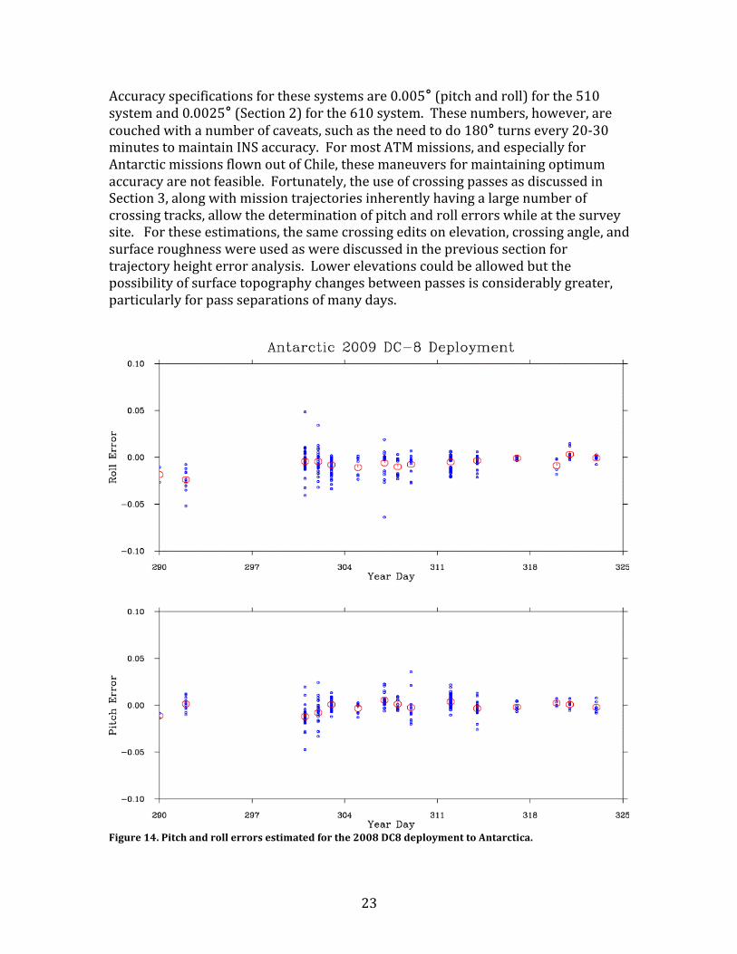
Figure 14. Pitch and roll errors estimated for the 2008 DC8 deployment to Antarctica.

24

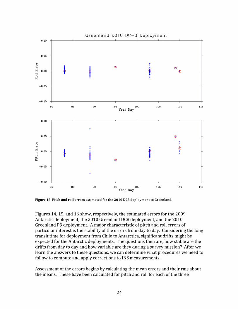
Figure 15. Pitch and roll errors estimated for the 2010 DC8 deployment to Greenland.

Figures 14, 15, and 16 show, respectively, the estimated errors for the 2009 Antarctic deployment, the 2010 Greenland DC8 deployment, and the 2010 Greenland P3 deployment. A major characteristic of pitch and roll errors of particular interest is the stability of the errors from day to day. Considering the long transit time for deployment from Chile to Antarctica, significant drifts might be expected for the Antarctic deployments. The questions then are, how stable are the drifts from day to day and how variable are they during a survey mission? After we learn the answers to these questions, we can determine what procedures we need to follow to compute and apply corrections to INS measurements. Assessment of the errors begins by calculating the mean errors and their rms about the means. These have been calculated for pitch and roll for each of the three

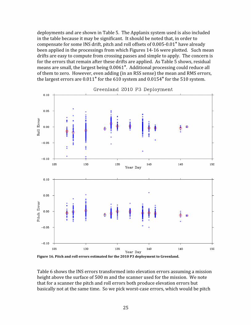
25

deployments and are shown in Table 5. The Applanix system used is also included in the table because it may be significant. It should be noted that, in order to compensate for some INS drift, pitch and roll offsets of 0.005-‐0.01° have already been applied in the processings from which Figures 14-‐16 were plotted. Such mean drifts are easy to compute from crossing passes and simple to apply. The concern is for the errors that remain after these drifts are applied. As Table 5 shows, residual means are small, the largest being 0.0061°. Additional processing could reduce all of them to zero. However, even adding (in an RSS sense) the mean and RMS errors, the largest errors are 0.011° for the 610 system and 0.0154° for the 510 system.

Figure 16. Pitch and roll errors estimated for the 2010 P3 deployment to Greenland.

Table 6 shows the INS errors transformed into elevation errors assuming a mission height above the surface of 500 m and the scanner used for the mission. We note that for a scanner the pitch and roll errors both produce elevation errors but basically not at the same time. So we pick worst-‐case errors, which would be pitch

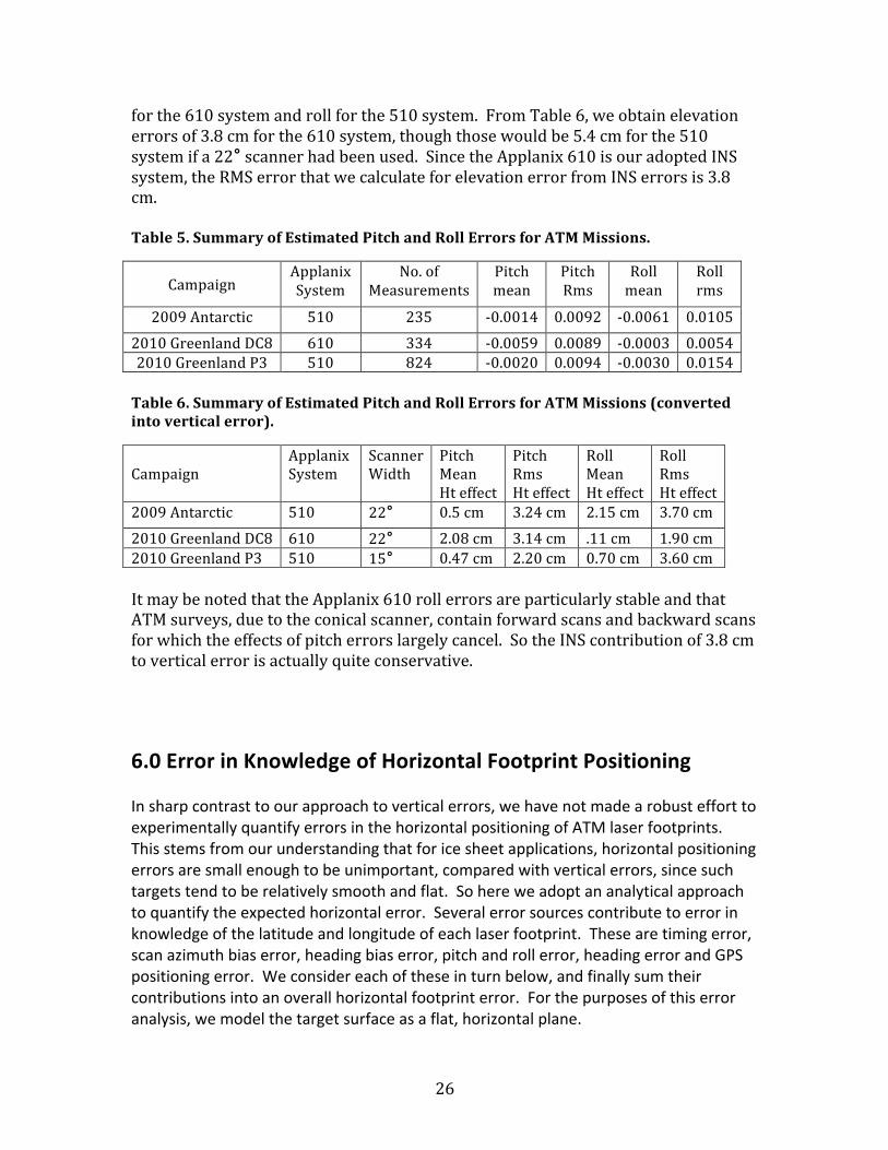
26

for the 610 system and roll for the 510 system. From Table 6, we obtain elevation errors of 3.8 cm for the 610 system, though those would be 5.4 cm for the 510 system if a 22° scanner had been used. Since the Applanix 610 is our adopted INS system, the RMS error that we calculate for elevation error from INS errors is 3.8 cm. Table 5. Summary of Estimated Pitch and Roll Errors for ATM Missions.

Campaign Applanix System

No. of Measurements

Pitch mean

Pitch Rms

Roll mean

Roll rms

2009 Antarctic 510 235 -‐0.0014 0.0092 -‐0.0061 0.0105 2010 Greenland DC8 610 334 -‐0.0059 0.0089 -‐0.0003 0.0054 2010 Greenland P3 510 824 -‐0.0020 0.0094 -‐0.0030 0.0154 Table 6. Summary of Estimated Pitch and Roll Errors for ATM Missions (converted into vertical error).

Campaign Applanix System

Scanner Width

Pitch Mean Ht effect

Pitch Rms Ht effect

Roll Mean Ht effect

Roll Rms Ht effect

2009 Antarctic 510 22° 0.5 cm 3.24 cm 2.15 cm 3.70 cm 2010 Greenland DC8 610 22° 2.08 cm 3.14 cm .11 cm 1.90 cm 2010 Greenland P3 510 15° 0.47 cm 2.20 cm 0.70 cm 3.60 cm It may be noted that the Applanix 610 roll errors are particularly stable and that ATM surveys, due to the conical scanner, contain forward scans and backward scans for which the effects of pitch errors largely cancel. So the INS contribution of 3.8 cm to vertical error is actually quite conservative.

6.0 Error in Knowledge of Horizontal Footprint Positioning In sharp contrast to our approach to vertical errors, we have not made a robust effort to experimentally quantify errors in the horizontal positioning of ATM laser footprints. This stems from our understanding that for ice sheet applications, horizontal positioning errors are small enough to be unimportant, compared with vertical errors, since such targets tend to be relatively smooth and flat. So here we adopt an analytical approach to quantify the expected horizontal error. Several error sources contribute to error in knowledge of the latitude and longitude of each laser footprint. These are timing error, scan azimuth bias error, heading bias error, pitch and roll error, heading error and GPS positioning error. We consider each of these in turn below, and finally sum their contributions into an overall horizontal footprint error. For the purposes of this error analysis, we model the target surface as a flat, horizontal plane.

27

6.1 Laser Pulse Timing Errors Waveform analysis can produce timing errors, as a point of the waveform corresponding to the target must be selected according to the algorithm described in Section 2.0. As mentioned in that section, an atmospheric refraction correction is added. Typical laser range timing measurements to a stationary target corrected for atmospheric refraction and system-‐timing biases result in ATM range RMS values of approximately 5 cm.

6.2 Scan and Date Timing Errors Timing errors arise because each laser shot is imperfectly time-‐tagged under the influence of two predominant kinds of motion. These are the forward motion of the aircraft in flight, and the motion of the scanner mechanism as it slews successive laser spots around the scan pattern. An error in time-‐tagging means that the laser spot on the ground is misplaced by an amount proportional to the speed of the motion. We show below that the dominant effect of timing errors is on the knowledge of scanner position. All timing in the ATM system is driven by a 1 pulse-‐per-‐second (1 PPS) strobe, which is produced by survey-‐grade GPS receivers. Prior to the 2010 ATM field season this 1 PPS strobe was provided by Ashtech Z-‐12 receivers, which had a stated 1 PPS accuracy of 1 microsecond. During the 2010 field season the ATM switched its timing source to newer Javad survey-‐grade GPS receivers, which have a rated 1 PPS timing accuracy of 25 nanoseconds. Between these 1 PPS strobes, all events, including scanner position, are timed using an internal crystal oscillator-‐based timing circuit, which has a rated stability of 50 ppm, or 50 microseconds per second. The 25-‐nanosecond 1 PPS error is negligible in comparison. We do not directly measure the angular position of the scan mirror. Instead, a Hall-‐effect sensor triggers a strobe when the scanner rotates past a fixed position at one point around each scan. We time-‐tag this strobe, and compute the angular position of the scanner for each similarly time-‐tagged laser pulse by linearly interpolating the 360° scan between these strobes. Thus, the maximum timing error for an individual laser pulse occurs at the end of each scan, just prior to the Hall-‐effect sensor being tripped to signal the beginning of a new scan. With 20 scans per second and the above 50 microseconds per second timing drift, this yields a maximum timing error during a scan of 2.5 microseconds, and an average timing error of half that, or 1.25 microseconds. The resulting average error in scanner position angle is 0.009°.

28

For the scanning motion on the ground, for this purpose we model the scan as a perfect circle with a diameter proportional to the sensor altitude above ground level (AGL). In truth the scan pattern is somewhat elliptical and slightly egg-‐shaped, but any error introduced by the circular approximation is small. In typical operations, the ATM is operated at an AGL altitude of 500 m with a scan rate of 20 Hz, and the resulting scan swath width for our wide-‐swath 22° scanner is 404 m. The corresponding circumference of the approximate circular scan is 1296 m, and the speed of the scan across the ground is 25,386 m/s. Given the average expected timing error above of 1.25 microseconds and resulting scanner position angle error of 0.009°, this yields a footprint position error of 3.2 cm. We neglect the timing-‐induced error due to forward motion of the aircraft, which at ~120 m/s is negligible compared to the 25,386 m/s scan motion.

6.3 Scan Azimuth Bias Error Scan azimuth bias error is a constant offset in knowledge of current angular position along the scan. It is a parameter that is estimated (along with pitch, roll and range biases) as part of the overall scanner calibration process. The combined least-‐squares determination of scanner parameters for the fall 2009 IceBridge deployment shown in Table 1 yields a formal uncertainty for the scan azimuth bias determination for that campaign as 0.027°. Since the least-‐squares process cannot formally model all potential sources of error, we conservatively double this formal uncertainty to an error estimate in scan azimuth bias of 0.05°. A displacement of a laser spot of 0.05° along the scan described above on the ground yields a horizontal position error of 18.0 cm.

6.4 Heading Bias Error Heading bias error is the fixed difference between the aircraft's true heading and the heading indicated by the ATM's inertial navigation system. Like scan azimuth bias, heading bias is estimated as part of the overall scanner calibration process. It is similar to, and mathematically correlated with, scan azimuth bias. However, since scan azimuth bias represents an error in the determination of where a spot lies along the scan while heading bias represents an angular displacement of the entire scan, the slightly non-‐circular shape of the scan helps to partially decorrelate the two parameters and allow their independent estimation. As before, the scanner parameter estimation process for Fall 2009 IceBridge shown in Table 1 yields a formal uncertainty in heading bias of 0.11°, which we again double to 0.2° for a conservative estimate of heading bias error. This relatively large displacement of the laser scan yields a horizontal position error of 72.0 cm.

29

6.5 Pitch and Roll Error Errors in knowledge of aircraft pitch and roll contribute to errors in horizontal footprint location by shifting the footprint location laterally according to the following trigonometric relationship:

dS = h*tan(theta+dtheta)-‐(w/2) (5)

where dS is the horizontal positioning error, h is AGL altitude, theta is the nominal off-‐nadir scan angle, dtheta is the error in knowledge of off-‐nadir angle, and w is the width of the full scan on the ground. Table 5 shows RMS pitch and roll errors for three IceBridge campaigns to be approximately 0.01° in almost every case, with mean errors considerably smaller. Based on that, we adopt 0.01° as the error in our knowledge of attitude. This yields a resulting horizontal positioning error of 10.2 cm.

6.6 Heading Error Heading error is distinct from heading bias error. It is the error in real-‐time knowledge of aircraft heading from the ATM's inertial navigation system. Where heading bias error remains fixed as long as the ATM transceiver and INS are themselves fixed to the airframe, heading error drifts in time as the INS drifts. Heading error is difficult to characterize from real-‐world ATM measurements simply because they are not very sensitive to it, particularly given the relatively smooth topography usually measured. However, we know that the Applanix 510 INS specifies pitch and roll error as 0.005° and heading as 0.008°. We also know from the above discussion of pitch and roll error that our real-‐world measurements of these are worse than these specifications by a factor of 2. Thus it seems reasonable to inflate the heading specification by a factor of 2 as well, then conservatively round up to 0.02°. Using the same geometrical argument as in sections 6.2 and 6.3, this yields a resulting horizontal error of 6.5 cm.

6.7 GPS Positioning Error Errors in horizontal GPS positioning of the aircraft translate directly into errors in horizontal laser spot positioning. In Section 4, the vertical GPS accuracy was shown to be <6 cm. GPS horizontal positioning is typically more accurate than vertical positioning for several reasons. For the current analysis, a value of 6 cm is adopted as the expected GPS horizontal accuracy, which is also the GPS contribution to horizontal laser spot positioning.

30

6.8 Total Horizontal Error The errors described above contribute to the overall horizontal error in footprint locations in an additive manner. Thus we compute the total error as the square root of the sum of the squares of these errors. Based on the above results, the overall horizontal error is 74 cm. It is dominated, by far, by the heading bias error, while timing, GPS and attitude errors are fairly insignificant in comparison. The precision of the horizontal spot locations is much better than this, however, because the largest error sources discussed above are constant biases. The remaining variable errors are the 2.9 cm timing error, the 6.5 cm heading error, the 9.3 cm pitch/roll error, and the 6 cm GPS positioning error. The square root of the sum of the squares of these is 14 cm.

7.0 Error Analysis Summary The various error components which affect the accuracy with which the ATM can perform topographic surveys for ice sheet elevation measurement have been discussed in some detail in previous sections and various accuracies estimated. Although sea ice tracks were not analyzed in the same way as ice sheets, because of the tide effects and lack of track crossings, they have been analyzed for attitude errors and the accuracies for them are expected to be comparable to those obtained for the ice sheets. The survey characteristics for the current primary ATM system, and the accuracies which have been estimated, are shown in Table 7. Perhaps the most significant accuracy, or at least the one with the most effort made to improve it, is vertical accuracy, which has 3 major contributors to its uncertainty:

● trajectory error, ● range bias error, and ● pointing errors

Trajectory error is currently the largest component. The attitude component is the next largest, and assumes that the most accurate currently available INS instrument will be employed. Even with this system, it is assumed that data taken during survey missions will be used for attitude verification and used, if necessary, to remove INS drifts that occur during transit from a base airbase to the survey region.

31

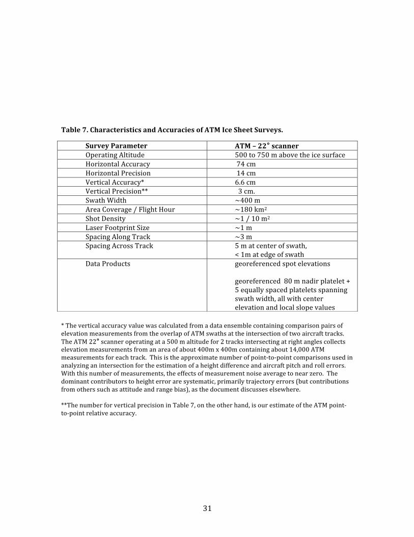
Table 7. Characteristics and Accuracies of ATM Ice Sheet Surveys.

* The vertical accuracy value was calculated from a data ensemble containing comparison pairs of elevation measurements from the overlap of ATM swaths at the intersection of two aircraft tracks. The ATM 22° scanner operating at a 500 m altitude for 2 tracks intersecting at right angles collects elevation measurements from an area of about 400m x 400m containing about 14,000 ATM measurements for each track. This is the approximate number of point-‐to-‐point comparisons used in analyzing an intersection for the estimation of a height difference and aircraft pitch and roll errors. With this number of measurements, the effects of measurement noise average to near zero. The dominant contributors to height error are systematic, primarily trajectory errors (but contributions from others such as attitude and range bias), as the document discusses elsewhere. **The number for vertical precision in Table 7, on the other hand, is our estimate of the ATM point-‐to-‐point relative accuracy.

Survey Parameter ATM – 22° scanner Operating Altitude 500 to 750 m above the ice surface Horizontal Accuracy 74 cm Horizontal Precision 14 cm Vertical Accuracy* 6.6 cm Vertical Precision** 3 cm. Swath Width ~400 m Area Coverage / Flight Hour ~180 km2 Shot Density ~1 / 10 m2 Laser Footprint Size ~1 m Spacing Along Track ~3 m Spacing Across Track 5 m at center of swath,

< 1m at edge of swath Data Products georeferenced spot elevations

georeferenced 80 m nadir platelet + 5 equally spaced platelets spanning swath width, all with center elevation and local slope values

32

8.0 References Krabill, W. B., R. H. Thomas, C. F. Martin, R. N. Swift, E. B. Frederick, 1995. Accuracy of airborne laser altimetry over the Greenland ice sheet, International Journal of Remote Sensing, 16(7) 1211-‐1222. DOI: 10.1080/01431169508954472 Krabill, W., E. Frederick, S. Manizade, C. Martin, J. Sonntag, R. Swift, R. Thomas, W. Wright, and J. Yungel, 1999. Rapid Thinning of Parts of the Southern Greenland Ice Sheet, Science 283 (5407), 1522. [DOI:10.1126/science.283.5407.1522] Krabill, W., W. Abdalati, E. Frederick, S. Manizade, C. Martin, J. Sonntag, R. Swift, R. Thomas, W. Wright, and J. Yungel, 2000. Greenland Ice Sheet: High-‐Elevation Balance and Peripheral Thinning, Science 289, 428-‐430 [DOI: 10.1126/science.289.5478.428] Krabill, W. B., W. Abdalati, E. B. Frederick, S. S. Manizade, C. F. Martin, J. G. Sonntag, R. N. Swift, R. H. Thomas, J. K. Yungel, 2002. Aircraft laser altimetry measurement of elevation changes of the Greenland ice sheet: technique and accuracy assessment, Journal of Geodynamics 34 357–376. [doi:10.1016/S0264-‐3707(02)00040-‐6] Martin, C. F., R. H. Thomas, W. B. Krabill, and S. S. Manizade, 2005. ICESat range and mounting bias estimation over precisely-‐surveyed terrain, Geophys. Res. Lett., 32, L21S07, doi:10.1029/2005GL023800.

REPORT DOCUMENTATION PAGE Form Approved OMB No. 0704-0188

The public repor ing burden for his collection of informa ion is estimated to average 1 hour per response, including the ime for reviewing instruc ions, searching existingdata sources, gathering and maintaining the data needed, and completing and reviewing the collec ion of information. Send comments regarding this burden estimate or any other aspect of this collection of information, including suggestions for reducing this burden, to Department of Defense, Washington Headquarters Services, Directorate for Information Operations and Reports (0704-0188), 1215 Jefferson Davis Highway, Suite 1204, Arlington, VA 22202-4302. Respondents should be aware that notwithstanding any other provision of law, no person shall be subject to any penalty for failing to comply with a collection of information if it does not display a currently valid OMB control number. PLEASE DO NOT RETURN YOUR FORM TO THE ABOVE ADDRESS. 1. REPORT DATE (DD-MM-YYYY) 2. REPORT TYPE 3. DATES COVERED (From - To)

4. TITLE AND SUBTITLE 5a. CONTRACT NUMBER

5b. GRANT NUMBER

5c. PROGRAM ELEMENT NUMBER

6. AUTHOR(S) 5d. PROJECT NUMBER

5e. TASK NUMBER

5f. WORK UNIT NUMBER

7. PERFORMING ORGANIZATION NAME(S) AND ADDRESS(ES) 8. PERFORMING ORGANIZATION REPORT NUMBER

9. SPONSORING/MONITORING AGENCY NAME(S) AND ADDRESS(ES) 10. SPONSORING/MONITOR'S ACRONYM(S)

11. SPONSORING/MONITORINGREPORT NUMBER

12. DISTRIBUTION/AVAILABILITY STATEMENT

13. SUPPLEMENTARY NOTES

14. ABSTRACT

15. SUBJECT TERMS

16. SECURITY CLASSIFICATION OF: 17. LIMITATION OF ABSTRACT

18. NUMBER OF PAGES

19b. NAME OF RESPONSIBLE PERSON

a. REPORT b. ABSTRACT c. THIS PAGE 19b. TELEPHONE NUMBER (Include area code)

Standard Form 298 (Rev. 8-98)Prescribed by ANSI Std. Z39-18

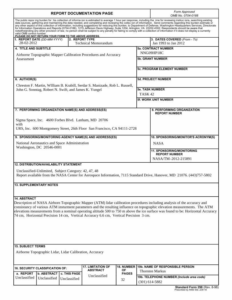
28-02-2012 Technical Memorandum Jan 1993 to Jan 2012


NNG09HP18C

TASK 42

Chreston F. Martin, WIlliam B. Krabill, Serdar S. Manizade, Rob L. Russell, John G. Sonntag, Robert N. Swift, and James K. Yungel

Sigma Space, Inc. 4600 Forbes Blvd. Lanham, MD 20706 with URS, Inc. 600 Montgomery Street, 26th Floor San Francisco, CA 94111-2728

National Aeronautics and Space Administration Washington, DC 20546-0001

NASA

NASA/TM–2012-215891

Unclassified-Unlimited, Subject Category: 42, 47, 48 Report available from the NASA Center for Aerospace Information, 7115 Standard Drive, Hanover, MD 21076. (443)757-5802

Description of NASA Airborn Topographic Mapper (ATM) lidar calibration procedures including analysis of the accuracy and consistancy of various ATM insturment parameters and the resulting influence on topographic elevation measurements. The ATM elevations measurements from a nominal operating altitude 500 to 750 m above the ice surface was found to be: Horizontal Accuracy 74 cm, Horizontal Precision 14 cm, Vertical Accuracy 6.6 cm, Vertical Precision 3 cm.

Airborne Topographic Lidar, Lidar Calibration, Accuracy

Unclassified Unclassified Unclassified Unclassified

32

Thorsten Markus

(301) 614-5882

Airborne Topographic Mapper Calibration Procedures and ... · Airborne Topographic Mapper...

Documents

Transcript of Airborne Topographic Mapper Calibration Procedures and ... · Airborne Topographic Mapper...