3

Air-Solids Flow Measurement Using Electrostatic Techniques

Jianyong Zhang Teesside University

UK

1.Introduction

1.1 Electrostatic charging and discharging

Many industrial processes such as coal pulverising, flour making, cement production, and fertiliser processing involve moving bulk solids by means of pneumatic conveying. Almost all particles become electrically charged during pneumatic transportation, which can be hazardous in industrial environment. The primary sources of electrification are frictional contact charging between particles, between particles and the conducting facility, charge transfer or sharing from one particle to another and charge induction.

Contact charging occurs at their common boundary when two dissimilar substances are brought into contact. On separation, each surface will carry an equal amount of charge with opposite polarity. Triboelectrification can be regarded as a complicated form of contact electrification in which there is transverse motion when two substances impinge or are rubbed together [1]. The transverse motion can in turn accentuate the charge transfer. Contact electrification occurs not only in pneumatic conveying, but also in milling, grinding, sieving and screw feeding.

Another source of electrostatic charge is induction. Charges will be induced on a conductor in an electrostatic field generated by charged particles. This conductor in turn changes the field distribution. If a conductor is insulated from the earth, its potential depends on the amount of charges, the permittivity of particles and their locations relative to the conductor [2]. The charge due to induction disappears when the charged particle moves away from the vicinity or sensing volume of the conductor as in pneumatic conveyance.

Charges can be shared by two particles when they collide to each other, or when one particle is settled on another. Charge sharing is more obvious between conductive particles.

Electrostatic charge can be recombined, for example via the earth or by contact with an object holding opposite charge. However charge on non-conductive particles can be retained and the relaxation time depends on the volume resistivity of bulk solids. If the volume resistivity is high, the charge could be retained even if the solids are in an earthed container. For particles suspended in pure gases as in pneumatic conveying, particles can remain charged for a long period of time irrespective of the particle material’s conductivity. Table 1 [3] shows the level of charge accumulation in particles, where the charge carried by unit mass of particle is given for solids of medium volume resistivity emerging from different processes.

www.intechopen.com

Electrostatics 62

Operation Mass charge density (C/kg)

Sieving 10-5-10-3

Pouring 10-3-10-1

Scroll feed transfer 10-2-1

Grinding 10-1-1

Micronising 10-1-102

Pneumatic conveying 10-1-103

Triboelectrical powder coating 103-104

Table 1. Charge build up on powder

Electrostatic charging can be a hazard if the charges are suddenly released via discharging to earth or another body, which produces a high local energy density and thus act as a possible ignition source. In section 7.2.4 of CENELEC and British Standard PD CLC/TR 50404: 2003, the discharges have been classified as “spark discharges”, “brush discharges”, “corona discharges”, “propagating brush discharges”, “cone discharges” and “lighting like discharges”. Among them, spark discharges, brush discharge and lighting like discharges may occur in pneumatic conveying. The incendivity of discharge is very much depends on the energy stored and the minimum ignition energy (MIE). Therefore the hazardousness of discharge depends on the area classification (zones) and gas group of process environment.

Potential build-up on metal items (pipe lines, flanges, bolts and etc) can be avoided by

earthing all these items. Sometimes pipe sections can become floated due to gaskets and

other insulators. Therefore it is important to bond such sections to the earthed sections. Care

must be taken when non-conductive pipes and hoses have to be used for pneumatic

conveying, the maximum possible energy stored must not exceed the MIE. In some case, it is

possible to choose the dense phase conveying which can reduce the risk of ignition inside

pipe due to lack of air. Different from one’s empirical knowledge, humidification is not

effective as a means of dissipating the charge from a dust cloud. The precaution for

electrostatic discharging is not the main focus in this chapter, more details can be found in

British and CENELEC Standard PD CLC/TR 50404:2003, “Electrostatics—code of practice

for the avoidance of hazards due to static electricity” [3].

1.2 Brief history of electrostatic techniques for air solid flow measurement

Electrostatic charging of flowing particles has long been known. The method to relate the magnitude of charge to the flow parameters was studied as early as in 1963. Batch, Dalmon and Hignett [4] used a pin probe to detect the current from the probe to earth in order to measure the mass flow rate of pneumatically conveyed pulverised fuel (p.f). The probe current depends on charge generated on probe due to contact electrification and induction.

The derivation of relations between the probe current and flow parameters was based on a

model developed by Cooper [5] and Hignett [6] which was for electrification of liquids in

motion.

Assume that the current flowing into the probe is I, the general relation is expressed as,

( , , , , , , )n PI f K d V M A (1.1)

www.intechopen.com

Air-Solids Flow Measurement Using Electrostatic Techniques 63

Where

--the electrical permittivity of particle

K--the electrical conductivity of particle

d--the particle diameter

V--the flow velocity in the region of the probe

--the density of air

M --the mass flow rate or flux of particle flow

AP--the cross-sectional area of probe

According to Pi Theorem [7], these variables may be expressed as four dimensionless

groups such that

2 2

2 4, ,n

P

I v d Mf

Kd A Kdd V

(1.2)

Then if the condition where only V and M vary, other parameters are assumed to be

constant, the above function can be simplified as

2

4 n

If M

V

(1.3)

At the time of research, the conclusion was that “the unique relation between probe current

and the p.f. flux (mass flow rate) cannot be obtained, thus the electrostatic probe cannot be

used as a means of determining the flux of p.f. in a pipe”. The method proposed by Batch et al

has been known as intrusive method which has been used by Hignett [8], and further explored

by Soo [9] and King [10]. A commercial product based on the same principle, which is

comprised of three probes installed with 120o gap apart, has been designed and manufactured

by TR-tech (now owned by Foster Wheeler) [11] [12].

King [10] has used non-intrusive method which measures the induced voltage on an insulated

pipe section (Pipe wall sensor), and he compared AC voltage measurement method to DC

measurement method [13] [14]. The AC or noise measurement method, also known as

“dynamic” method [15] takes the AC signal component to indicate flow concentration.

Coulthard applied this technique to coal flow measurement in the Methil power station in

Scotland [16], and Gajewski has employed it to measure dust in motion [17]. Gajewski further

studied the measuring mechanism by combining the electrostatic field theory with electrical

circuit analysis for a lined circular pipe wall sensor [18]. Since 1970s, positive and convincing

results have been reported for measuring a range of different particles, e.g. pf, glass beads,

sands and polymer granules, which encouraged further study in this area.

The mechanism of electrostatic metering system has been studied by many people, for

example, Gajewski [19], Massen [20] and Hammer [21] studied filtering effect of the circular

electrode, and Yan investigated charge induction based on free space electrostatic field

www.intechopen.com

Electrostatics 64

theory [15]. When the Finite Element Method became practically viable with the increased

speed and capacity of computers, more in depth study of charge induction became possible.

A model describing the relation between the induced charge on an insulated pipe section

(electrode) and the charge carried by a particle with respect of its location, known as

“Spatial sensitivity” was established by Cheng [22]. This model was developed based on

electrostatic field theory using the Finite Element method (FEM). Based on the above model,

and with further study, Zhang [23] has related flow concentration and solids mass flow rate

to the charge level on electrodes by employing stochastic process theory. He also

investigated and verified 2-D spatial sensitivity of ring-shaped electrode to “roping” flow

[24] and effects of particle size [25] on the charge carried by particles. The effects of velocity

and concentration have been studied experimentally and theoretically since then [26].

Cheng’s model [22] has also been used by Xu [27], and an exploitation of frequency method

for velocity measurement has also been based on the Cheng’s model [28] [29]. The product

operating according to dynamic electrostatic techniques with trade name PfMaster has been

developed and manufactured by ABB Ltd.

2. Charge induction and “dynamic” measurement method

2.1 Mathematic model for charge induction

In this section, the main focus of the analysis will be on the meters with circular electrodes. For the analysis of other types of electrostatic sensors, the same principles apply. The method adopted here is based on the analysis conducted by Cheng [22].

Fig.1 depicts a simplified, schematic view of circular electrostatic meter. The circular metallic electrode is installed flush with, and electrically insulated from the inner surface of the earthed pipe, but exposed to the medium inside the pipe. This arrangement ensures that the electrode is sensitive to the charges carried by particles without restricting flow and can avoid severe charge build-up on non-conductive lining. It also minimises the electrode wear that can occur with intrusive probes [30]. The charge generated on the electrode is due to the following effects:

1. particle contacting with the electrode, and 2. charge induction due to the presence of charged particles within the sensing volume.

Since the speed of charged particle through the sensing volume is insignificant compared to the speed of light, so the electromagnetic effect generated by flowing charged solids can be neglected. The analysis therefore is under the assumption of a pure electrostatic electrical field. The electrode is narrow compared to the pipe diameter, so the contact charge between particle and electrode was not considered. The model presented here is also assumed a lean phase flow regime, under which effect of dielectric property of solids on the electrostatic field is neglected.

The principle of the measurement can be approximately (but not accurately) explained as follows: Regarding the entire conveying pipe (ignoring the insulator) as an enclosed system, the total charge induced on the inner surface of the system should equal to the charge carried by the source particle, but of opposite polarity. The portion of the total induced charge on the electrode varies with the location of the particle (although total charge induced on the inner surface of the enclosed system does not vary).

www.intechopen.com

Air-Solids Flow Measurement Using Electrostatic Techniques 65

Fig. 1. Charge induction

For the convenience of calculation, assume a non-conductive, negatively charged particle surrounded by air as the only source of electrostatic field.

In order to know the induced charge Q on the electrode, the charge density on the inner

surface of the electrode, , needs to be found.

S

Q ds (1.4)

where S stands for the entire inner surface area of the electrode, s is the surface area variable.

According to the electrostatic theory, the surface charge density is equal to the electric flux density (electric displacement) D, i.e.

D (1.5)

D (1.6)

D E (1.7)

E (1.8)

is the gradient operator, E is the electrical field strength, , the relative permittivity of the

medium and refers to as the electrical potential.

From equations 1.5 to 1.8, Equation 1.9 and 1.10 can be derived,

D E (1.9)

( ) (1.10)

Assume the following boundary conditions

( ) 0 ( ) 0 ( ) 0P i t (1.10)

www.intechopen.com

Electrostatics 66

where P, I, t represent the boundaries of the earthed conveying pipe, the insulator and the electrode respectively.

The conveying pipe is earthed, so the potential on it is zero. The electrode is usually connected to a charge amplifier in which the electrode is virtually earthed, the potential on electrode is very close to zero. It may be noticed that the potential on the insulator is hard to set. In the simulation, it was set as zero, and other low voltages (2, and 3Volts) on the insulator the similar results were obtained.

The problem becomes to find the potential . If the potential distribution is known, the

charge density on the inner surface of electrode can be found, hence the induced charge on

the electrode can be derived from Equation 1.4. This is a 3-D problem. The location of

charged particle affects the amount of induced charge on the electrode. However in a

cylindrical co-ordinate, if the particle only changes it angular co-ordinate with its radial (r)

and axial (x) coordinates keeping unchanged, the induced charge on the electrode should

not change due to the symmetrical configuration of the system. Consider also the

superposition theorem in electrostatic field, a 2-D model is sufficient for solving this 3-D

problem, and a ring-shaped charge situated with its axis coinciding with the pipe central

line will produces the same induced charge on the electrode as a point particle carrying the

same amount of charge at the same axial and radial locations. The equivalent ring was used

by Cheng to calculate the charge induction as shown in Fig.2.

Fig. 2. Charge Induction

The detailed analysis can be found in [22]. Here provided is an equation relating the charge induction and source charge and its location, also known as “spatial sensitivity” which was obtained from FEM simulation and regression.

2kxQ Ae (1.11)

where Q is the charge induced on the electrode due to a point charged particle carrying unit

charge located at (x, r, ), but Q depends on r and x only. A and k are two parameters determined by electrode geography, namely W/R ratio (where W is the width of electrode, and R the radius of the sensor) and radial location r of the charged particle.

www.intechopen.com

Air-Solids Flow Measurement Using Electrostatic Techniques 67

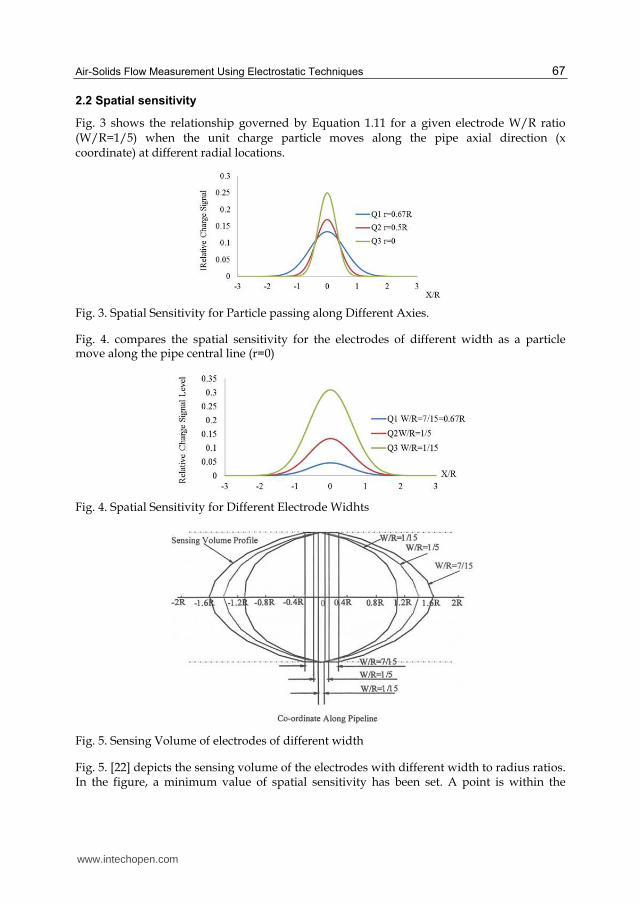
2.2 Spatial sensitivity

Fig. 3 shows the relationship governed by Equation 1.11 for a given electrode W/R ratio (W/R=1/5) when the unit charge particle moves along the pipe axial direction (x coordinate) at different radial locations.

Fig. 3. Spatial Sensitivity for Particle passing along Different Axies.

Fig. 4. compares the spatial sensitivity for the electrodes of different width as a particle move along the pipe central line (r=0)

Fig. 4. Spatial Sensitivity for Different Electrode Widhts

Fig. 5. Sensing Volume of electrodes of different width

Fig. 5. [22] depicts the sensing volume of the electrodes with different width to radius ratios. In the figure, a minimum value of spatial sensitivity has been set. A point is within the

www.intechopen.com

Electrostatics 68

sensing zone if the spatial sensitivity at that point is above this value. The shape of sensing volume depends on the geometry of the electrode.

If the particle movement along the axial direction is the main concern, the velocity of the

particle in this direction can be related to Equation 1.11 by replacing x with Vt, where V is the particle velocity along the pipe axial direction, t is time.

2 2kV tQ Ae (1.12)

This temporal expression relates the time, axial velocity and induced charge together, where for a given electrode, A and k vary with radius location r only. The radial velocity component of particle is not considered. The recent research on analysis of radial velocity can be found in [31].

The Fourier transform of Equation 1.12 provides the frequency property of the electrode to a

point charge moving at velocity V along the pipe line.

2 2kV tQ F Q F Ae

Therefore,

2

1

4k VAQ e

V k

(1.13)

The analysis conducted by Cheng [22] is presented above. Different from the previous analysis, the model in Equation 1.11 has taken the presence of metal conveying pipe (earthed), the insulator between the conveyor and electrode, and the effect of resultant charge on the electrode into account. The significances of this model are that it allows studying the effects of sensor geometry and velocity on charge induction, and permits the frequency analysis. From this model, 2-D and 3-D spatial sensitivity profiles of a sensor can be derived. Equation 1.11 was the first such expression to be used for temporal and frequency domain analysis and it can be used as a guide for sensor design.

2.3 Dynamic measurement

As reviewed in section 1, King [10] compared AC and DC measurement methods for both circular sensor (he named it as “pipe sensor”) and pin sensor (intrusive probe). In industrial environment, DC signal on electrodes is more prone to interference so the fluctuation of induced charge has been used for measurement. An electrostatic metering system which measures the signal fluctuation is termed unofficially “dynamic” measurement system, although in the author’s view, the word “dynamic” has been misused. In such a system, it is the change or variation of the induced signal that matters. The fluctuation produced by air-solids flow is regarded as band-limited white noise [13] proportional to solids concentration [32]. The fluctuation in number of particles, random movement of particles, particle size and shape changes can also result in the random change in signal level. The signal level is dependent upon mass flow rate or concentration for given mean velocity, the distribution of particle size, humidity and etc.

www.intechopen.com

Air-Solids Flow Measurement Using Electrostatic Techniques 69

3. Measurement of velocity and mass flow rate

3.1 Unit impulse response of ring-shaped electrode

Equations 1.11 1.12 and 1.13 provide the temporal and frequency spatial responses of a circular electrostatic meter to a charged particle. Zhang [23] extended these models to study the response to flow concentration and flow mass flow rate. In order to simplify the analysis, it is assumed that the particles of uniform size are evenly distributed over the sensing volume so that the volume concentration of solids is determined only by the number of particles per unit volume, i.e. N. Because the solids are fed or dropped into the conveying system at an upstream point, so that N and solids concentration can be regarded as a waveform travelling along pipe line at velocity V. The point of injection is the source of the wave. Hereafter the number of particles per unit volume and concentration will be respectively denoted as N(x,t) and Con(x,t), both of which depend on x, the axial distance and t, the time. The charge induced on the electrode, Q, is a function of N(x,t) in Equation 1.14 or a function of Con(x, t) as in Equation 1.15.

2 22 -k(r) xrA(r)N(x,t)e n

Vol

Q G D drdx (1.14)

2 2-k(r) xr

A(r)Con(x,t)e ( )Rm Vol

G rQ d dx

RD

(1.15)

where N(x, t) is the waveform of the number of particles which varies along the pipeline at a

given time, and at any point of x, it varies with time; is a constant for a given diameter of sensor. A and k depend on radius r for an electrode of a given width; Gn and G are constants related to particle surface charge density and pipe geometry. Con(x,t) is the concentration waveform, and R is the radius of the electrode.

In order to find the unit impulse response of the electrode, let Con(x,t) be a delta function, i.e.

( , ) ( )x

Con x t tV

(1.16)

thus there is only one non-zero point at any given time in the co-ordinate x which is V*t ( or at given point x, the impulse arrives at time x/V). Under such a concentration, the induced charge is the unit impulse response of the electrode. From Equation1.15, we have

2 2

1( ) ( * )

0

( ) ( ) k r V t

m

G r rQ h t A r e d

R RD

(1.17)

and the Fourier transfer function of the electrode is

2

2

1( / ) 112

( )4

0

( ) ( )( )

( ) ( )

k rV

m

Q G r A r rH e d

Con R RDV k r

(1.18)

where Q() is the Fourier transfer function of the induced charge, and the Con() is the Fourier transfer function of the concentration.

www.intechopen.com

Electrostatics 70

3.2 Equivalent circuit and charge amplifier

The signal induced on the electrode has to be connected to a measuring equipment or a preamplifier. Usually the input impedance of a preamplifier or a measurement equipment is finite, therefore the characteristics of the sensor comprising the electrode and the connected electronics depend not only on the electronics but also on the internal impedance of the electrode due to “loading effect”.

Fig. 6. Sensing system

Although there are various types of preamplifier circuits, the charge preamplifier is among

those of most widely used for such systems. As shown in Fig.6 the electrode is at virtual

earth potential. The capacitance CF in the feedback loop is used to suppress the effects of the

wiring capacitance and the equivalent capacitance Cn, when the values of the wiring

capacitance and Cn as well as their variation have to be considered. RF is used to provide a

DC path, which also determines the lower cut-off frequency with CF.

The charge amplifier blocks DC component of the signal Q, so the system measures signal

fluctuation, performing “dynamic” measurement.

The transfer function of the measurement system T() is

( ) ( )( )

( ) ( ) ( )( ) ( ) ( )

o oU UQT H P

Con Con Q

(1.19)

where Uo() is the output voltage of the charge amplifier, P() is the transfer function of the

charge amplifier. The loading effect of source is reflected in P() which depends on Cn and rn.

3.3 Measuring solids mass flow rate

Assume the concentration signal is a band-limited white noise, based on equation 1.19,

Zhang [23] has used Parseval’s formula to relate the rms of Uo to the fluctuation in

concentration,

2

2

max

rmsrms

conU V (1.20)

www.intechopen.com

Air-Solids Flow Measurement Using Electrostatic Techniques 71

If the root mean square conrms of the flow noise con(t) is directly proportional to the mean

solids concentration ( )Con t , Urms, the rms value of the sensor’s output has a linear

relationship with the mean solids concentration for given solids density and particle size.

The above analysis assumes that the net charge carried by solids does not depend upon velocity. Hence the velocity in Equation 1.20 reflects the effect of velocity on characteristics of the sensing system only. The amount of net charge carried by particles is actually affected by velocity. Gajewski [17] has studied the this effect on the ‘charging tendency’ of PVC dust, and Masuda conducted the tests on several different materials and found that the

electrostatic meter’s output was proportional to V [14], where varied from 1.4-1.9. The effect of velocity on the net charge has also been confirmed from many tests on pulverized coal [33].

If we assume the net charge is proportional to the solids velocity over the range

investigated, as it was suggested by Gajewski [17] for PVC dust over the velocity range

below 20m/s, equation 1.20 becomes

2

2 3

max

rmsrms

conU V or 3/2

maxmax

rmsrms

con VU V M (1.21)

where max is the signal frequency up limit, M is the solids mass flow rate. Hence the root

mean square value of signal can be used to directly measure solids mass flow rate if the effect of velocity has been compensated.

3.4 Velocity measurement

In Equations 1.20 and 1.21, it can be seen that, to achieve accurate concentration or flow rate

measurement result, the effect of velocity needs to be compensated for, therefore, the

velocity measurement cannot be avoided.

There are several different ways to measure velocity of conveyed solids, however, the cross correlation method remains the most practical and viable one. Since late 1960s and early 1970s, the cross-correlation found its applications in flow measurement. Various sensors have been used to measure different types of flow. A cross correlatior detects the flow noise transit time, from which the mean velocity of flow can be derived. Beck [34], Coulthard [35], Cole [13] and King [10] used this method to measure velocity of multi-phase flow. Keech and Coulthard realised a microprocessor based electrostatic cross correlator for the ABB cable meter [36]. Cheng adopted “polarity cross correlation” to measure pulverised coal flow velocity in a blast furnace [37]. The technique has been further improved to accommodate multi-channel velocity measurement [38].

In electrostatic air-solids flow measurement system, usually two identical electrodes are mounted up and down stream with a known distance apart. If the flow concentration Con(t) is rectilinearly transferred from upstream to downstream at a velocity V, it can be expected that the signal from the downstream electrode is a delayed replica of the signal from the upstream electrode, i.e.

2 1 1Con t Con t L / V Con (t t) , (1.22)

www.intechopen.com

Electrostatics 72

where L is the distance between two electrode. is the transit time.

Because L is known, thus once is found, the velocity V can be determined from Equation 1.23

V L / t. (1.23)

According to the definition, the cross-correlation function between Con1(t) and Con2(t) is equal to

1 2 1 2

0

1( ) lim Con t Con t dt Tc c

TR

T (1.24)

If the two signals are exactly identical,

1 2 1 1

0

1( ) lim Con t Con t L / V dt Tc c

TR

T (1.25)

The cross correlation becomes a delayed version of auto correlation of Con1(t), as shown in Fig. 7.

Fig. 7. Cross Correlation

1 2 1 1

( ) ( / ) ( / )c c c c ccR R L V R L V (1.26)

In reality, two signals are not exactly identical, however the cross correlation efficient can be very high. Even for low cross correlation coefficient, say, 0.5, a cross correlator can still successfully capture the flow transit time and find the average flow velocity. The frequency band of the signal determines the measurement accuracy of transit time, which in turn affects the accuracy of velocity measurement.

4. Relative measurement

The response of an electrostatic meter for air solids flow measurement depends on density, particle size, velocity, mass flow rate and flow profile. Over the past ten years, the performance of dynamic electrostatic meters has been significantly improved, however the high measurement accuracy is still not achievable if all the above parameters vary over wide ranges.

In many cases, only two or three parameters vary and other parameters stay relatively stable. This is particularly true in coal-fired power station, where pulverised fuel comes

www.intechopen.com

Air-Solids Flow Measurement Using Electrostatic Techniques 73

from a mill and split into six or eight conveyors. Under normal conditions, the density of solids, moisture content and even flow profile are similar in different conveyors, but particle size distribution, mass flow rate and velocity vary from one conveyor to another. If the system can provide the signal proportional to the split (relative or percentage of overall mass flow rate) with velocity and particle size compensation, the mass flow rate in each conveyor can be given with reasonable accuracy because the overall loading entering the mill is known.

4.1 Signal, concentration, mass flow rate and velocity

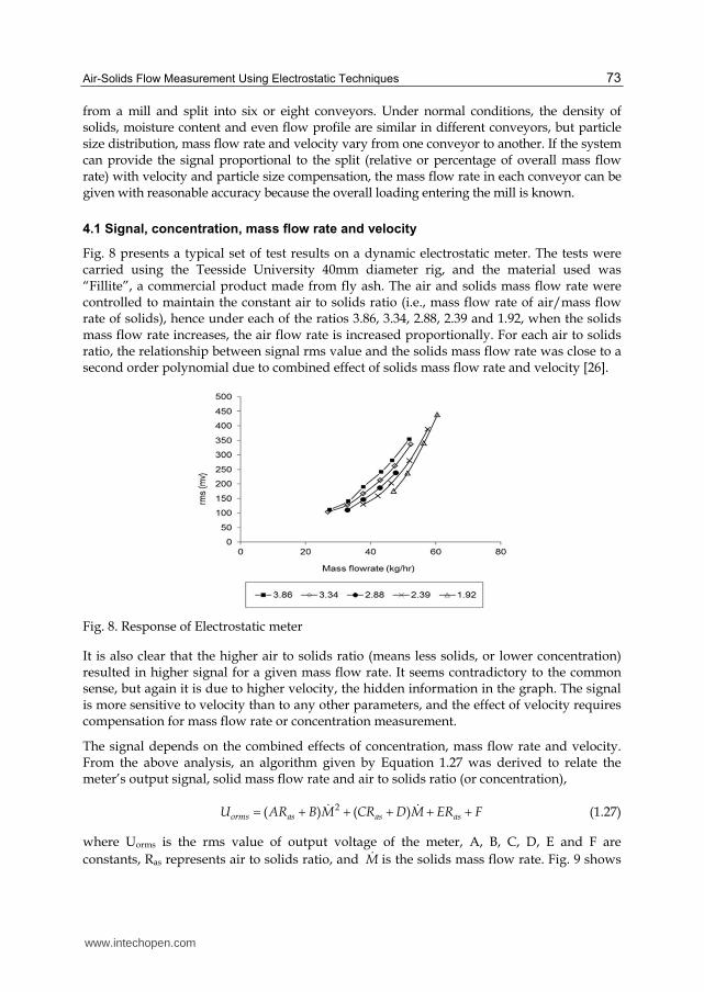
Fig. 8 presents a typical set of test results on a dynamic electrostatic meter. The tests were carried using the Teesside University 40mm diameter rig, and the material used was “Fillite”, a commercial product made from fly ash. The air and solids mass flow rate were controlled to maintain the constant air to solids ratio (i.e., mass flow rate of air/mass flow rate of solids), hence under each of the ratios 3.86, 3.34, 2.88, 2.39 and 1.92, when the solids mass flow rate increases, the air flow rate is increased proportionally. For each air to solids ratio, the relationship between signal rms value and the solids mass flow rate was close to a second order polynomial due to combined effect of solids mass flow rate and velocity [26].

Fig. 8. Response of Electrostatic meter

It is also clear that the higher air to solids ratio (means less solids, or lower concentration) resulted in higher signal for a given mass flow rate. It seems contradictory to the common sense, but again it is due to higher velocity, the hidden information in the graph. The signal is more sensitive to velocity than to any other parameters, and the effect of velocity requires compensation for mass flow rate or concentration measurement.

The signal depends on the combined effects of concentration, mass flow rate and velocity. From the above analysis, an algorithm given by Equation 1.27 was derived to relate the meter’s output signal, solid mass flow rate and air to solids ratio (or concentration),

2( ) ( )orms as as asU AR B M CR D M ER F (1.27)

where Uorms is the rms value of output voltage of the meter, A, B, C, D, E and F are

constants, Ras represents air to solids ratio, and M is the solids mass flow rate. Fig. 9 shows

www.intechopen.com

Electrostatics 74

the measured mass flow rate against the true mass flow rate for various velocities and air to

solids ratios [26].

Fig. 9. Calibration Graph

4.2 Effect of particle size

As discussed from the beginning of this chapter, the induced charge on the insulated electrode is a function of several factors including particle size.

From Equations 1.15, 1.17, 1.18, it can be seen that induced charge on electrode is inversely proportional to particle size. It is due to the fact that the mass of solids is proportional to D3 and the total surface area of solids is proportional to D2 for spherical particles, where D is particle diameter. If surface charge density is a constant, larger surface of total particles will provide higher signal level when the particles are getting smaller [25].

Fig. 10. Signal Vs particle size

www.intechopen.com

Air-Solids Flow Measurement Using Electrostatic Techniques 75

Fig. 10 was obtained from experiments using sieved materials [39]. For the given mass flow

rate, velocity and concentration, the signal from a dynamic electrostatic meter decreased

with particle size for the size above 250 µm, confirming Equation 1.15, 1.17 and 1.18.

However for particles below that size, the signal reversed the trend, i.e. the smaller particle

size resulted in lower signal. At the time of experiment, the signal drop for smaller particles

was thought to be caused by the sudden change in solids flow rate. The recent research

revealed that the signal drop for small particles could have been caused by flow regime

change. When the size of particle is getting smaller, the flow becomes less turbulent. This effect

outweighs the effect of total particle surface area increase so that overall signal level decreases.

4.3 Spatial sensitivity

In pneumatically conveyed air solid flow, the distribution of solid phase is often un-even.

For example around bends and restrictive devices, the roping flow regime may be formed.

The air solids flow profiles depend on conveying velocity, particle size, humidity and

geometry of conveyor. The research in this area can be found elsewhere [40][41][42].

The measurement results will be affected by flow regime unless a meter has a uniform spatial sensitivity.

Fig. 11. Spatial Sensitivity Test Results

Fig.11 depicts the test results obtained on a 14” (356mm) diameter electrostatic meter [24]. A

roping stream of constant flow rate was provided with an one-inch jet, the roping stream

was parallel to the pipe axial central line and moved cross the pipe cross sectional area along

its diameter. The material used was pulverised coal. The output voltage (rms) of the meter

to the “roping” flow stream was recorded when the jet moved from the centre to a location

very close to pipe wall. The signals on the wide electrode (Red W/R=0.5) and on the narrow

electrode (Blue W/R=0.014) followed the same trend. It is clear that the signal increased

with the flow stream getting closer to the pipe wall, and then it started to drop as the roping

stream crossing about 70% of full radius, which is caused by combination of the increased

sensitivity and the reduced sensitive volume of the sensor as shown in Figs 3, 4 and 5.

www.intechopen.com

Electrostatics 76

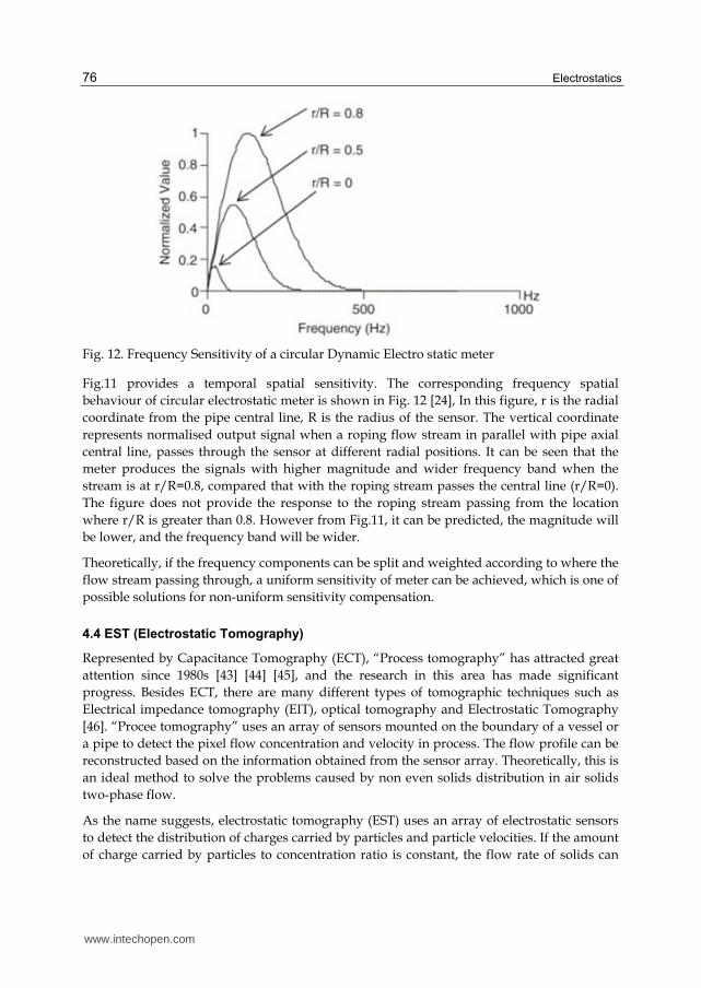
Fig. 12. Frequency Sensitivity of a circular Dynamic Electro static meter

Fig.11 provides a temporal spatial sensitivity. The corresponding frequency spatial

behaviour of circular electrostatic meter is shown in Fig. 12 [24], In this figure, r is the radial

coordinate from the pipe central line, R is the radius of the sensor. The vertical coordinate

represents normalised output signal when a roping flow stream in parallel with pipe axial

central line, passes through the sensor at different radial positions. It can be seen that the

meter produces the signals with higher magnitude and wider frequency band when the

stream is at r/R=0.8, compared that with the roping stream passes the central line (r/R=0).

The figure does not provide the response to the roping stream passing from the location

where r/R is greater than 0.8. However from Fig.11, it can be predicted, the magnitude will

be lower, and the frequency band will be wider.

Theoretically, if the frequency components can be split and weighted according to where the

flow stream passing through, a uniform sensitivity of meter can be achieved, which is one of

possible solutions for non-uniform sensitivity compensation.

4.4 EST (Electrostatic Tomography)

Represented by Capacitance Tomography (ECT), “Process tomography” has attracted great

attention since 1980s [43] [44] [45], and the research in this area has made significant

progress. Besides ECT, there are many different types of tomographic techniques such as

Electrical impedance tomography (EIT), optical tomography and Electrostatic Tomography

[46]. “Procee tomography” uses an array of sensors mounted on the boundary of a vessel or

a pipe to detect the pixel flow concentration and velocity in process. The flow profile can be

reconstructed based on the information obtained from the sensor array. Theoretically, this is

an ideal method to solve the problems caused by non even solids distribution in air solids

two-phase flow.

As the name suggests, electrostatic tomography (EST) uses an array of electrostatic sensors

to detect the distribution of charges carried by particles and particle velocities. If the amount

of charge carried by particles to concentration ratio is constant, the flow rate of solids can

www.intechopen.com

Air-Solids Flow Measurement Using Electrostatic Techniques 77

then be derived based on the integration of the product of pixel concentration and velocity

over a given cross sectional area.

For any type of process tomography, the successful realization depends on sensing system design, signal conditioning, signal to noise (S/N) ratio, proper data acquisition system and efficient algorithm.

EST is a passive sensing system, which is one of its advantages [47] over ECT. However inherently, for the same number of sensors (electrodes), the resolution of EST is lower than that of ECT. Combined systems (dual modality) [48] can offer better resolution and reliability. Fig. 13 provides the simulation results for an EST and an EST/ECT combined systems [2]. In this figure, a uniform positive charge density distribution in a stratified flow at the bottom half of a pipe is assumed, the reconstructed image using information from the EST system only in Fig.13b is vague, the boundary is not clear. Compared to the image in Fig.13b, Fig.13c offers much better result which is obtained by combining the information from the EST and ECT of dual modality system.

(a) (b) (c)

Fig. 13. Image Reconstruction from an EST/ECT

5. Current research in this area

At present, the modelling of charge induction with consideration of particle dielectric

property is the new development in this area [2]. The research to develop an overall model

to relate the signal rms, solids velocity and solids mass flow rate is under way [26]. The

electrostatic method used in square pipe lines [49] has also been investigated, and the study

on the effect of radial velocity on flow measurement is useful for understanding of the

mechanism of electrostatic meters [31]. The technique of combing ECT and EST for gas

solids flow measurement opened a new frontier.

At the time of writing this chapter, the electrostatic technique have been successful in some

areas, for example in measuring flow split among pneumatic conveyors, in providing

warning of blockage and for inferring primary air flow rate measurement . Some research

outcomes are yet to be applied in practice. It is envisaged that the techniques will be further

improved for flow measurement and flow regime diagnose not only in lean-phase

conveying as in coal-fire power generation, but also for dense phase flow as in gasification

and in blast furnace feeding.

www.intechopen.com

Electrostatics 78

6. References

[1] Dechene. R.L., Farmer A.D., ‘ Triboelectricity—A tool for solids flow measurement’, Industrial Minerals, May 1992, pp131-135

[2] Zhou Bin, Zhang Jianyong, Wang Shimin, “Image reconstruction in electrostatic tomography using a priori knowledge from ECT”, Nuclear Engineering and Design Volume 241, Issue 6, June 2011, pp 1952-1958.

[3] British Standard, BSI PD CLC/TR 50404:2003, “Electrostatics—Code of practice for the avoidance of hazards due to static electricity”, Published on 9 July 2003.

[4] Batch B.A., Dalmon J. and Hignett E.T., “An Electrostatic probe for measuring the particle flux in two-phase flow”, Laboratory note No. RD/L/N115/63, Central Electrcity Research Laboratories, 7 November 1963

[5] Cooper W.E., “The electrification of fluids in motion”, British Journal of Physics 4 Suppl.No. 2, 1953 Couvertier. P. 1961, C.R. Akad.Sci., 252 No. 12, 1726-7

[6] Hignett, E.T. 1963, Ph.D. Thesis, University Of Liverpool. [7] Curtis, W.D., Logan, J.D., Parker, W.A., “Dimensional analysis and the pi theorem”,

Linear Algebra and Its Applications, 1982, 47 (C), pp. 117-126 [8] Hignett E.T., “Particle-charge magnitudes in electrostatic precipitation”, PROC. IEE,

vol.114, No.9, September 1967, pp1325-1328. [9] Soo S.L., Tung S.K., “Pipe flow of suspensions in turbulent fluid - Electrostatic and

gravity effects” Applied Scientific Research, Volume 24, Issue 1, December 1971, Pages 83-97.

[10] P. W. King, 1973) "Mass flow measurement of conveyed solids by monitoring of intrinsic electrostatic noise levels", Proc. 2nd Int. Conf. on the Pneumatic Transport of Solids in Pipes PNEUMOTRANSPORT 2, University of Surrey, Guildford, England, pp 9-19 , 1973

[11] Bindemann K. C. G., Miller D. & Hayward P., (1999). “Kingsnorth pf flow meter demonstration trials”. DTI Report Coal R167.

[12] Foster Wheeler Power Group Inc, “New ECT STAR makes On-line Coal Flow Measurement even more powerful”, Design Bulletin, No 109.5 November 2002.

[13] Cole B. N., Baum M. R., Mobbs F.R., ‘An investigation of electrostatic charging effects in High-speed gas-solids Pipe flows’, Proc. Instn. Mech. Engres. Vol 184 , 1969-70, pp77-83.

[14] Masuda Hiroaki, Komatsu Takahiro, Mitsui Naohiro and Iinoya Koichi, “Electrification of gas-solid suspensions in Steel and insulating-coated pipes”, Journal of Electrostatics, Volume 2, 1976-1977-pp341-350

[15] Yan Y. “Mass flow measurement of pneumatically conveyed solids”, Ph .D thesis, University of Teesside 1992.

[16] Coulthard J., “solids flow measurement using ring-shaped electrostatic sensors”,Industrial report to Davy McKee Stockton, June 1983.

[17] Gajewski J.B.and Szaynok A., “Charge measurement of dust particles in motion”, Journal of Electrostatics, Volume 10, 1981, pp229-234.

[18] Gajewski J.B., Szaynok A., “ Charge measurement of particles in motion, part I, J. Electrostatics, 10 (1998) pp229-234

[19] Gajewski J.B., Glòd B.J., Kala W.S., “Electrostatic method for measuring the two-phase pipe flow parameters”, IEEE Transactions on Industry Applications, Volume 29, No.3, May/Jue 1993, pp 650-654.

www.intechopen.com

Air-Solids Flow Measurement Using Electrostatic Techniques 79

[20] Massen R., ‘Sensor with coded apertures’, J. Phys. E: Sci. Instrum. Vol. 20, 1987, pp409-416 [21] Hammer E. A., Green R. G., ‘The spatial filtering effect of capacitance transducer

electrodes’, J. Phys. E: Sci. Instrum., Vol.16, 1983, pp 438-443 [22] Cheng Ruixue, “ A study of Electrostatic Pulverised Fuel Meters”, Ph. D thesis, Teesside

University, 1996. [23] Zhang Jianyong, “A Study of an Electrostatic Flow Meter”, Ph. D thesis, Teesside

University, 2002. [24] Zhang Jianyong, Coulthard John, “Theoretical and experimental studies of the

sensitivity of an electrostatic pulverised fuel meter”, Journal of Electrostatics, Vol.63, issue 12, pp 1133-1149, OCT. 2005.

[25] Zhang Jianyong, Coulthard John, “On-line Indication of Variation of Particle Size Using Electrostatic PF Meters”, The proceedings of the 31st International Technical Conference on Coal Utilization & Fuel Systems, Clearwater, Florida, USA, May 21 to 25 2006.

[26] Zhang Jianyong; Cheng Ruixue; Coulthard John, “Calibration of an electrostatic flow meter for bulk solids measurement in pneumatic transportation”, Bulk Solids Handling 28 (5), pp. 314-319, 2008

[27] Xu C. “Gas-solids Two phases Flows Parameters and Particle Electrostatic Measurement”, Ph D thesis, Souheast University, Nanjing, China, 2005

[28] Xu C., Tang G., Zhou B., Yang D., Zhang J., and Wang S., “Electrostatic introduction theory based spatial filtering method for solid particle velocity measurement”, AIP Conference Proceedings ,Volume 914, 2007, Pages 192-200.

[29] Zhang Jianyong; Cheng Ruixue; Al-Sulaiti Ahmed, “Velocity Measurement of Pneumatically Conveyed Solids Based on Signal Frequency Spectrum”, 8th International Conference on measurement and control of Granular Materials, Shenyang, China, 27-29 Aug. 2009

[30] Laux S., Grusha J, Rosin T., Kersch J.D., “ECT: More than just coal-flow monitoring”, Modern power systems, March 2002, pp 22-29.

[31] Zhang Jianyong; Zhou Bin;Wang Shimin; “Effect of axial and radial velocities on solids mass flow rate measurement”, Robotics and Computer-Integrated Manufacturing, volume 26, Issue 6, December 2010, pp 576-582

[32] Gajewski J.B., “Electric charge measurement in pneumatic installations”, Journal of Electrostatics, Volume 40-41, 1997, pp 231-236

[33] ECSC Project 7220-PR-050 Report: Powergen, U. Teesside, Sivus, ABBCS, IST ISTCM, ABB Kent , “Measurement & control techniques for improving combustion efficiency & reducing emissions from coal-fired plant”, 2002.

[34] Beck M. S., Plaskowski A., ‘How Inherent flow noise can be used to measure mass flow of granular materials’, Instrument Review, November 1967, pp 458-461

[35] Coulthard J, “Ultrasonic Cross-correlation Flowmeters”, Ultrasonics,Volume 11, Issue 2, 1973, March, 1973

[36] Coulthard J., Keech R.P., Asquith P., “The Electrostatic Cable meter”, Inst. Of Physics International Conference on Electrostatics”, York May 1995.

[37] Cheng R.，Wang S.C.” Microprocessor based on-line real time cross correlator for two-

phase flow measurement”) Transactions of University of Science and Technology, Beijing, China.1991,13(6).-572-576, (In Chinese)

www.intechopen.com

Electrostatics 80

[38] Keech ray, Coulthard John, Cheng Ruixue, “Measurement using cross correlation”, Patent No WO/1998/055839, filed 06 May 1998, International Application No. PCT/GB1998/001654, publication date, 10.12.1998.

[39] Zhang Jianyong, “Project Final report (RFCS-CR-03005) On-line measurement of coal quality parameters by inference of sensor information”, for the work carried by Teesside University, Dec. 2007

[40] N. Huber and M. Sommerfield, Characterization of the cross-sectional particle concentration in pneumatic conveying system. Powder Technol., 79 (1994), pp. 91–210.

[41] Frank Th., Bernert K., Pachler K., Schneider H., “Aspects of efficient parallelization of disperse gas-particle flow prediction using Eulerian–Lagrangian approach”, Proceedings of ICMF-2001, Fourth International Conference on Multiphase Flow, May 21–June 1, 2001 New Orleans, LA, USA, paper 311.

[42] Peng B., Zhang C., Zhu J., “Numerical study of the effect of the gas and solids distributors on the uniformity of the radial solids concentration distribution in CFB risers”,Powder Technology,Volume 212, Issue 1, 15 September 2011, Pages 89-102

[43] Wang, H., Wang, X., Lu, Q., Sun, Y., Yang, W., “Imaging gas-solids distribution in cyclone inlet of circulating fluidised bed with rectangular ECT sensor”, 2011 IEEE International Conference on Imaging Systems and Techniques, IST 2011 - Proceedings, art. no. 5962181, pp. 55-59

[44] Williams, R.A., Beck, M.S. “Process Tomography - State of the Art”, Proceedings of the first World Congress on Industrial Process Tomography, Buxton, UK , 1999, pp. 357-362.

[45] Yang W.Q. , Stott A.L , Beck M.S. , Xie C.G. , “Development of capacitance tomographic imaging systems for oil pipeline measurements”, Review of Scientific Instruments, Volume 66, Issue 8, 1995, Pages 4326-4332

[46] Green R.G., Rahmat M. F., Evans K., Goude A., Henry M., and Stone J. A. R., "Concentration profiles of dry powders in a gravity conveyor using an electrodynamic tomography system", Meas. Sci. Technol., vol. 8, no. 2, pp.192 - 197 , 1997.

[47] Machida M., Kaminoyama M., “Sensor design for development of tribo-electric tomography system with increased number of sensors”, Journal of Visualization, Volume 11, Issue 4, 2008, Pages 375-385.

[48] Basarab-Horwath I., Daniels, A.T., Green, R.G. “Image analysis in dual modality tomography for material classification”, Measurement Science and Technology, Volume 12, Issue 8, August 2001, PP 1153-1156.

[49] Peng Lihui, Zhang Y. Yan Y., “Characterization of electrostatic sensors for flow measurement of particulate solids in square-shaped pneumatic conveying pipelines”, Sensors and Actuators A: Physical, Volume 141, Issue 1, 15 January 2008, Pages 59-67

www.intechopen.com

ElectrostaticsEdited by Dr. Hüseyin Canbolat

ISBN 978-953-51-0239-7Hard cover, 150 pagesPublisher InTechPublished online 14, March, 2012Published in print edition March, 2012

InTech EuropeUniversity Campus STeP Ri Slavka Krautzeka 83/A 51000 Rijeka, Croatia Phone: +385 (51) 770 447 Fax: +385 (51) 686 166www.intechopen.com

InTech ChinaUnit 405, Office Block, Hotel Equatorial Shanghai No.65, Yan An Road (West), Shanghai, 200040, China

Phone: +86-21-62489820 Fax: +86-21-62489821

In this book, the authors provide state-of-the-art research studies on electrostatic principles or include theelectrostatic phenomena as an important factor. The chapters cover diverse subjects, such as biotechnology,bioengineering, actuation of MEMS, measurement and nanoelectronics. Hopefully, the interested readers willbenefit from the book in their studies. It is probable that the presented studies will lead the researchers todevelop new ideas to conduct their research.

How to referenceIn order to correctly reference this scholarly work, feel free to copy and paste the following:

Jianyong Zhang (2012). Air-Solids Flow Measurement Using Electrostatic Techniques, Electrostatics, Dr.Hüseyin Canbolat (Ed.), ISBN: 978-953-51-0239-7, InTech, Available from:http://www.intechopen.com/books/electrostatics/air-solids-flow-measurement-using-electrostatic-techniques

© 2012 The Author(s). Licensee IntechOpen. This is an open access articledistributed under the terms of the Creative Commons Attribution 3.0License, which permits unrestricted use, distribution, and reproduction inany medium, provided the original work is properly cited.