Air Pollution and Mortality: Estimating Regional and ... · Air Pollution and Mortality: Estimating...

Air Pollution and Mortality: Estimating Regional andNational Dose–Response Relationships

Francesca Dominici, Michael Daniels, Scott L. Zeger, and Jonathan M. Samet

We analyzed a national data base of air pollution and mortality for the 88 largest U.S. cities for the period 1987–1994, to estimate relativerates of mortality associated with airborne particulate matter smaller than 10 microns (PM10) and the form of the relationship betweenPM10 concentration and mortality. To estimate city-speci� c relative rates of mortality associated with PM10 , we built log-linear modelsthat included nonparametric adjustments for weather variables and longer term trends. To estimate PM10 mortality dose–response curves,we modeled the logarithm of the expected value of daily mortality as a function of PM10 using natural cubic splines with unknownnumbers and locations of knots. We also developed spatial models to investigate the heterogeneity of relative mortality rates and ofthe shapes of PM10 mortality dose–response curves across cities and geographical regions. To determine whether variability in effectestimates can be explained by city-speci� c factors, we explored the dependence of relative mortality rates on mean pollution levels,demographic variables, reliability of the pollution data, and speci� c constituents of particulate matter. We implemented estimation withsimulation-based methods, including data augmentation to impute the missing data of the city-speci� c covariates and the reversible jumpMarkov chain Monte Carlo (RJMCMC) to sample from the posterior distribution of the parameters in the hierarchical spline model. Wefound that previous-day PM10 concentrations were positively associated with total mortality in most the locations, with a 05% incrementfor a 10 Œg/m3 increase in PM10 . The effect was strongest in the Northeast region, where the increase in the death rate was twice ashigh as the average for the other cities. Overall, we found that the pooled concentration–response relationship for the nation was linear.

KEY WORDS: Air pollution; Data augmentation; Generalized additive model; Hierarchical model; Natural cubic spline; Particulatematter; Relative rate.

1. INTRODUCTION

Epidemiologic time series studies conducted in cities aroundthe world have consistently found associations between dailylevels of airborne particulate matter smaller than 10 microns(PM10), and daily numbers of deaths. These � ndings haveraised concern about the public health effects of PM pollu-tion (Schwartz 1994; Pope, Dockery, and Schwartz 1995a;American Thoracic Society and Bascom 1996a, 1996b), andmotivated reassessment of air quality standards in many coun-tries, including the United States, the United Kingdom, andthe European Union members. However, one key limitationof these studies has been use of data from a single or a few,possibly nonrepresentative, locations. The National Morbidity,Mortality, and Air Pollution Study (NMMAPS) addresses thislimitation by assembling and analyzing a national data basethat includes information on mortality, weather, and air pollu-tion for the 88 largest metropolitan areas in the United States.The statistical framework estimates associations between airpollution and mortality (and morbidity) for the entire UnitedStates, within large regions and for particular cities (Samet,

Francesca Dominici is Assistant Professor, Department of Biostatistics,Bloomberg School of Public Health, The Johns Hopkins University, Balti-more, MD 21205 (E-mail: [email protected]). Michael Daniels is AssistantProfessor, Department of Statistics, Iowa State University, Ames, IA (E-mail:[email protected]). Scott L. Zeger is Professor and Chairman, Departmentof Biostatistics, Johns Hopkins University, Baltimore, MD 21205 (E-mail:[email protected]). Jonathan M. Samet is Professor and Chairman, Depart-ment of Epidemiology, Johns Hopkins University, Baltimore, MD 21205 (E-mail: [email protected]). The research described in this article was partiallysupported by a contract and grant from the Health Effects Institute (HEI), anorganization jointly funded by the Environmental Protection Agency (EPA;R824835) and automotive manufacturers. The contents of this article do notnecessarily re� ect the views and policies of HEI, EPA, or motor vehicleor engine manufacturers. Funding for Francesca Dominici was provided bythe HE Is Walter A. Rosenblith New Investigator Award. Funding of MichaelDaniels was provided by National Science Foundation grant DMS9816630.Funding was also provided by Johns Hopkins Center in Urban Environmen-tal Health grant 5P30ES03819-12. The authors thank John Bachmann of theEPA for kindly providing us with the data on particulate matter composition,Giovanni Parmigiani for comments and suggestions on the statistical models,and Ivan Coursac for assistance with data base development.

Zeger, Dominici, Dockery, and Schwartz 1999; Samet et al.2000b).

Initially, we analyzed data for the 20 largest U.S. cities,using a two-stage linear regression model for combining evi-dence from multiple locations (Dominici, Samet, and Zeger2000). We then extended this analysis to estimate the shape ofthe PM10 mortality dose–response curve (Daniels, Dominici,Samet, and Zeger 2000). The 20-city analyses were con-strained in model development and in their substantive � nd-ings by the relatively small number of cities. Further investi-gation is needed into the heterogeneity of the dose–responserelationship of air pollution and mortality across cities andregions and on the modi� cation of the effects of PM10 by fac-tors such as copollutants, PM composition, city or regionalmeasurement error, and population characteristics and suscep-tibilities.

In this article we extend the NMMAPS data base and anal-yses to include the 88 largest U.S. cities. The objectives ofthis article are (1) to combine information across these 88locations to estimate regional and national relative rates ofmortality from exposure to PM10, (2) to explore heterogeneityof effects across broad geographic regions and determinantsof heterogeneity, and (3) to estimate regional and nationalair pollution mortality dose–response curves. To determinewhether city-speci� c factors can explain variability in the rel-ative rates of mortality for PM10, we have collected data on aset of city-speci� c variables: demographic characteristics, co-pollutant levels, precision of the air pollution measurements,and particle size distribution. A subset of these city-speci� cvariables are missing in some cities, and thus a strategy forimputing missing data is needed. To address objectives (1)and (2), we develop a three-stage linear regression model withdata augmentation to handle missing data in the city-speci� c

© 2002 American Statistical AssociationJournal of the American Statistical Association

March 2002, Vol. 97, No. 457, Applications and Case Studies

100

Dominici et al.: Air Pollution and Mortality 101

covariates. To address (3), we use a two-stage spline model toestimate the shape of the PM10 mortality dose–response curveswithin each region.

Section 2 describes the data base of air pollution, mor-tality, and meteorological data from 1987 to 1994 for the88 U.S. cities used in this analysis. Section 3 introducesthe hierarchical regression model with data augmentation forcombining information on the PM10 mortality associationsacross cities within regions and across regions. Section 4introduces the hierarchical spline model used to estimateregional and national PM10 mortality curves. Section 5 sum-marizes the � ndings and presents results of model compar-isons, model checking, and sensitivity to prior distributions.Finally, Section 6 discusses our � ndings. Details on the imple-mentation of the reversible jump Morkov Chain Monte Carlo(RJMCMC) for model � tting are presented in the Appendix.

2. DATA

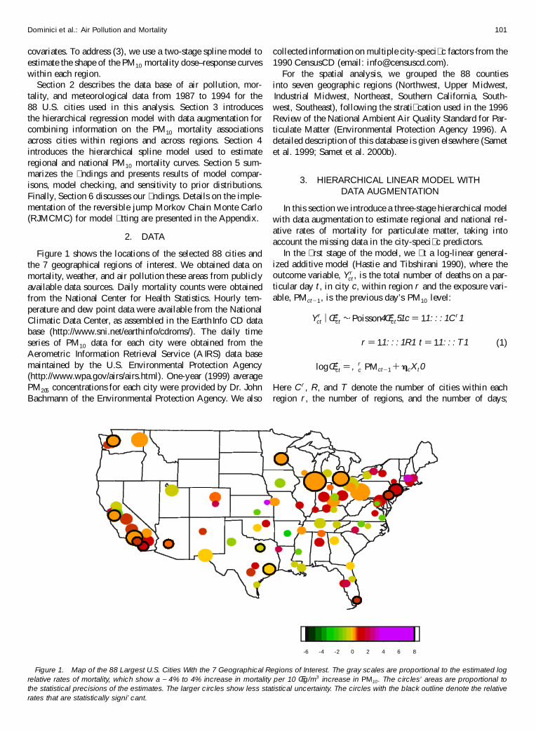
Figure 1 shows the locations of the selected 88 cities andthe 7 geographical regions of interest. We obtained data onmortality, weather, and air pollution these areas from publiclyavailable data sources. Daily mortality counts were obtainedfrom the National Center for Health Statistics. Hourly tem-perature and dew point data were available from the NationalClimatic Data Center, as assembled in the Earth Info CD database (http://www.sni.net/earthinfo/cdroms/). The daily timeseries of PM10 data for each city were obtained from theAerometric Information Retrieval Service (A IRS) data basemaintained by the U.S. Environmental Protection Agency(http://www.wpa.gov/airs/airs.html). One-year (1999) averagePM205 concentrations for each city were provided by Dr. JohnBachmann of the Environmental Protection Agency. We also

-6 -4 -2 0 2 4 6 8

Figure 1. Map of the 88 Largest U.S. Cities With the 7 Geographical Regions of Interest. The gray scales are proportional to the estimated logrelative rates of mortality, which show a - 4% to 4% increase in mortality per 10 Œg/m3 increase in PM10 . The circles’ areas are proportional tothe statistical precisions of the estimates. The larger circles show less statistical uncertainty. The circles with the black outline denote the relativerates that are statistically signi’ cant.

collected information on multiple city-speci� c factors from the1990 CensusCD (email: [email protected]).

For the spatial analysis, we grouped the 88 countiesinto seven geographic regions (Northwest, Upper Midwest,Industrial Midwest, Northeast, Southern California, South-west, Southeast), following the strati� cation used in the 1996Review of the National Ambient Air Quality Standard for Par-ticulate Matter (Environmental Protection Agency 1996). Adetailed description of this database is given elsewhere (Sametet al. 1999; Samet et al. 2000b).

3. HIERARCHICAL LINEAR MODEL WITHDATA AUGMENTATION

In this section we introduce a three-stage hierarchical modelwith data augmentation to estimate regional and national rel-ative rates of mortality for particulate matter, taking intoaccount the missing data in the city-speci� c predictors.

In the � rst stage of the model, we � t a log-linear general-ized additive model (Hastie and Tibshirani 1990), where theoutcome variable, Y r

ct , is the total number of deaths on a par-ticular day t, in city c, within region r and the exposure vari-able, PMctƒ1, is the previous day’s PM10 level:

Y rct

— Œrct Poisson4Œr

ct51 c D 11 : : : 1C r 1

r D 11 : : : 1R1 t D 11 : : : T 1 (1)

logŒrct

D ‚rc PMctƒ1 C ÇcXt 0

Here C r , R, and T denote the number of cities within eachregion r , the number of regions, and the number of days;

102 Journal of the American Statistical Association, March 2002

Œrct

D E6Y rct7; Xt is the tth row of the design matrix for the

confounding factors (e.g., long-term trends and seasonality inthe mortality time series, and weather variables); and Çc is thecorresponding vector of coef� cients. The potential confound-ing variables and the rationale for their inclusion, are listed inTable 1. Justi� cation for selecting the smooth functions to con-trol for longer-term trends, seasonality, and weather and sen-sitivity analyses with respect to the lag structure of the expo-sure variable have been given by Samet, Zeger, and Berhane(1995), Samet, Zeger, Kelsall, Xu, and Kalkstein (1997), Kel-sall, Samet, and Zeger (1997), Samet, Dominici, Curriero,Coursac, and Zeger (2000a), and Dominici et al. (2000).

In several locations, a high percentage of days had missingPM10 values for which measurements are generally requiredonly every six days. Because there are missing values of somepredictor variables are missing on some days, we restrictedanalyses to days with no missing values across the full set ofpredictors.

At the second stage, we describe the heterogeneity of thecity-speci� c effects within regions, assuming that

Âr — � r01Á1 Zr 1‘ 2 NCr 4�

r0 jr C Zr Á1‘ 2I51

r D 11 : : : 1R1 (2)

where Âr D 6‚r11 : : : 1‚r

C r 7 is the collection of true PM10 coef� -cients for the C r cities in region r , Zr is a matrix of dimensionC r � p with the cth row 6Zr

c11 : : : 1 Zrcp7 denoting the cen-

tered covariates for the cities belonging to region r , �r0 is the

regional air pollution effect when all of the covariates are cen-tered at their mean values, jr is a vector of length C r havingall elements equal to 1, and Á D 6�11 : : : 1 �p7 is the vector ofthe second-stage regression coef� cients (i.e., � j measures thechange in ‚r

c per unit of change in the city-speci� c covariateZr

cj), and ‘ 2 measures the variance of the ‚rc’s within each

region. The second-stage covariates are included in the designmatrix Z, and the rationale for their inclusion are summa-rized in Table 2. Details on the exploratory analyses that ledto the selection of these variables appear elsewhere (Samet etal. 2000b).

At the third stage of the model, we investigated heterogene-ity of the regional air pollution effects 4� r

05 across regions; weassume

� r0

— �01 ’ 2 N �01 ’ 2¢0 (3)

Here �0 is the overall relative rate of mortality for PM10, and’ 2 measures the variance of � r

0 across regions.

Table 1. Potential Confounding Factors in the Estimation of the City-Speci’ c Relative Rates Associated WithParticulate Air Pollution Levels, and the Rationale for Their Inclusion in the Model

Predictors Primary reasons for inclusion

Indicator variables for the three age groups To allow for different baseline mortality rates within each age groupIndicator variables for the day of the week To allow for different baseline mortality rates within each day of the weekSmooth functions of time with 7 degrees of freedom (df)/yr To adjust for long-term trends and seasonalitySmooth functions of temperature with 6 df To control for the known effects of weather on mortalitySmooth functions of dewpoint with 3 df To control for the known effects of humidity on mortalitySeparate smooth functions of time (2 df/yr) for each age group

contrastTo separately adjust for seasonality within each age group

Because the vector Çc corresponding to the factors listed inTable 1 is highly dimensional (its dimension is 118), the com-putational demand of a full Bayesian approach—that is, sim-ulating from the joint posterior distributions of ‚r

c and Çc andthen integrating over the Çc to obtain the marginal posteriordistributions of the ‚r

c—is extremely laborious. The compu-tation becomes even more intensive when we implement dataaugmentation to impute the missing city-speci� c covariates.Therefore, let OÂr D 6 O‚r

11 : : : 1 O‚rCr 7 and V r D diag4vr

11 : : : 1 vrCr 5

be the maximum likelihood estimates (MLEs); their samplingvariances are obtained by � tting the city-speci� c model (1) forcity c and region r . We simplify the computation substantiallyby replacing the � rst stage of the model with the MLE-basednormal approximation to the likelihood function,

OÂr NC r 4Âr 1 V r 50 (4)

Because of the large number of days with air pollution andmortality measurements within each city, we found that theMLE-based normal approximation to the likelihood is ade-quate, as discussed in Section 5.1.

This analysis is complicated by missing data for the second-stage variables in a subset of cities. (The percentages of citieswith missing data for each variable are listed in Table 2.)We impute the missing data by implementing data augmen-tation (Tanner 1991) within the Gibbs sampler (Gelfand andSmith 1990), which requires speci� cation of the conditionaldistributions of vectors of covariates that are missing (Zr

cm )given the vector of covariates that are observed (Zr

co). Weassume that

Zrcm

— Zrco1È1 è Nlc

4Ìo1èmm0o51 (5)

where

ÌoD Èm

C èmoèƒ1oo 4Zr

coƒ Èo51

èmm0oD èmm

ƒ èmoèƒ1oo èom

and Ì and è are the mean and covariance matrix of the p vec-tor Zr

cD 6Zr

cm1Zrco7.

The model speci� cation is completed with the selection ofprior distributions for the parameters at the top level of thehierarchy. We assume a priori that these parameters are inde-pendent, and, except for the within-region and between-regionvariance components (‘ 2 and ’2), we choose vague conju-gate priors with large variances. For ‘ 2 and ’2, we assumea half-normal prior distribution, which gives moderate weightto complete homogeneity while also allowing for the possi-bility of more substantial heterogeneity (Pauler and Wake� eld


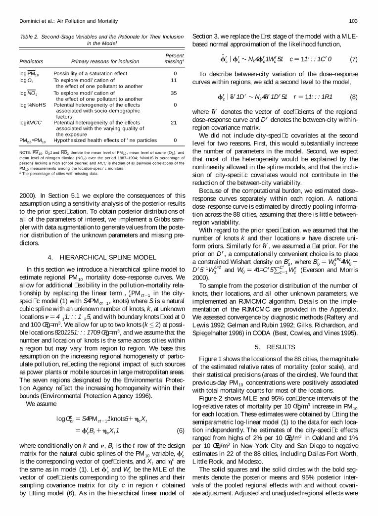
Table 2. Second-Stage Variables and the Rationale for Their Inclusionin the Model

PercentPredictors Primary reasons for inclusion missinga

log PM10 Possibility of a saturation effect 0log SO3 To explore modi’ cation of 11

the effect of one pollutant to anotherlog NO2 To explore modi’ cation of 35

the effect of one pollutant to anotherlog %NoHS Potential heterogeneity of the effects 0

associated with socio-demographicfactors

logitMCC Potential heterogeneity of the effects 21associated with the varying quality ofthe exposure

PM205=PM10 Hypothesized health effects of ’ ne particles 0

NOTE: PM10 , SO31 and NO2 denote the mean level of PM10 , mean level of ozone (O3), andmean level of nitrogen dioxide (NO2) over the period 1987–1994; %NoHS is percentage ofpersons lacking a high school degree; and MCC is median of all pairwise correlations of thePM10 measurements among the location-speci’ c monitors.a The percentage of cities with missing data.

2000). In Section 5.1 we explore the consequences of thisassumption using a sensitivity analysis of the posterior resultsto the prior speci� cation. To obtain posterior distributions ofall of the parameters of interest, we implement a Gibbs sam-pler with data augmentation to generate values from the poste-rior distribution of the unknown parameters and missing pre-dictors.

4. HIERARCHICAL SPLINE MODEL

In this section we introduce a hierarchical spline model toestimate regional PM10 mortality dose–response curves. Weallow for additional � exibility in the pollution–mortality rela-tionship by replacing the linear term ‚r

cPMctƒ1 in the city-speci� c model (1) with S4PMctƒ1, knots) where S is a naturalcubic spline with an unknown number of knots, k, at unknownlocations Í D 4�11 : : : 1 �k5, and with boundary knots � xed at 0and 100 Œg=m3. We allow for up to two knots (k µ 2) at possi-ble locations 8201251 : : : 1 709 Œg=m3, and we assume that thenumber and location of knots is the same across cities withina region but may vary from region to region. We base thisassumption on the increasing regional homogeneity of partic-ulate pollution, re� ecting the regional impact of such sourcesas power plants or mobile sources in large metropolitan areas.The seven regions designated by the Environmental Protec-tion Agency re� ect the increasing homogeneity within theirbounds (Environmental Protection Agency 1996).

We assume

logŒrct

D S4PMctƒ11 knots5C ÇcXt

D ÔrcBt

C ÇcXt1 (6)

where conditionally on k and Í, Bt is the t row of the designmatrix for the natural cubic splines of the PM10 variable, Ôr

c

is the corresponding vector of coef� cients, and Xt and Çc arethe same as in model (1). Let OÔr

c and W rc be the MLE of the

vector of coef� cients corresponding to the splines and theirsampling covariance matrix for city c in region r obtainedby � tting model (6). As in the hierarchical linear model of

Section 3, we replace the � rst stage of the model with a MLE-based normal approximation of the likelihood function,

OÔrc

— Ôrc Nk4Ô

rc1W r

c 51 c D 11 : : : 1 C r 0 (7)

To describe between-city variation of the dose–responsecurves within regions, we add a second level to the model,

Ôrc

— Är 1Dr Nk4Är 1 Dr 51 r D 11 : : : 1 R1 (8)

where Är denotes the vector of coef� cients of the regionaldose–response curve and Dr denotes the between-city within-region covariance matrix.

We did not include city-speci� c covariates at the secondlevel for two reasons. First, this would substantially increasethe number of parameters in the model. Second, we expectthat most of the heterogeneity would be explained by thenonlinearity allowed in the spline models, and that the inclu-sion of city-speci� c covariates would not contribute in thereduction of the between-city variability.

Because of the computational burden, we estimated dose–response curves separately within each region. A nationaldose–response curve is estimated by directly pooling informa-tion across the 88 cities, assuming that there is little between-region variability.

With regard to the prior speci� cation, we assumed that thenumber of knots k and their locations Í have discrete uni-form priors. Similarly for Är , we assumed a � at prior. For theprior on Dr , a computationally convenient choice is to placea constrained Wishart density on Br

0 , where Br0

D W 1=20 4W0

CDr 5ƒ1W 1=2

0 and W0 D 41=C r5PC r

cD1 W rc (Everson and Morris

2000).To sample from the posterior distribution of the number of

knots, their locations, and all other unknown parameters, weimplemented an RJMCMC algorithm. Details on the imple-mentation of the RJMCMC are provided in the Appendix.We assessed convergence by diagnostic methods (Raftery andLewis 1992; Gelman and Rubin 1992; Gilks, Richardson, andSpiegelhalter 1996) in CODA (Best, Cowles, and Vines 1995).

5. RESULTS

Figure 1 shows the locations of the 88 cities, the magnitudeof the estimated relative rates of mortality (color scale), andtheir statistical precisions (areas of the circles). We found thatprevious-day PM10 concentrations were positively associatedwith total mortality counts for most of the locations.

Figure 2 shows MLE and 95% con� dence intervals of thelog-relative rates of mortality per 10 Œg/m3 increase in PM10

for each location. These estimates were obtained by � tting thesemiparametric log-linear model (1) to the data for each loca-tion independently. The estimates of the city-speci� c effectsranged from highs of 2% per 10 Œg/m3 in Oakland and 1%per 10 Œg/m3 in New York City and San Diego to negativeestimates in 22 of the 88 cities, including Dallas-Fort Worth,Little Rock, and Modesto.

The solid squares and the solid circles with the bold seg-ments denote the posterior means and 95% posterior inter-vals of the pooled regional effects with and without covari-ate adjustment. Adjusted and unadjusted regional effects were


seattlesanjoseoaklanddenver

sacramentosalt lake city

tacomastockton

colorado springmodestospokaneolympia

regional-unadjustedregional-adjusted

phoenixsanantonio

oklandel pasoaustin

albuquerquecorpus christi

lubbockregional-unadjustedregional-adjusted

los angelessandiego

santa anaheimsanbernardino

riversidefresno

bakersfieldregional-unadjustedregional-adjusted

minneapoliskansas city

wichitades moineskansas city

topekaregional-unadjustedregional-adjusted

chicagodetroit

clevelandpittsburghsant louis

buffalocolumbuscincinnati

indianapolislouisvilledaytonakron

grand rapidstoledo

madisonfort waynelexingtonevansville


new yorkphiladelphia

newarkbaltimorerochesterworcester

bostondc

providencejersey citysyracusenorfolk

richmondarlingtonkingston


dallashoustonmiamiatlanta

st petersburghtampa

memphisorlando

jacksonvillebirmingham

charlottenashville

tulsanew orleans

raleighbaton rouge

little rockgreensboro

knoxvilleshreveport

jacksonhuntsville

regional-unadjustedregional-adjustedoverall-unadjustedoverall-adjusted

regional-adjusted

regional-adjusted

regional-adjusted

regional-adjusted

regional-adjusted

regional-adjusted

regional-adjusted

regional-unadjusted

regional-unadjusted

regional-unadjusted

regional-unadjusted

regional-unadjusted

regional-unadjusted

regional-unadjusted

northwest

southwest

southcal

uppermidwest

industmidwest

northeast

southeast

%increase in mortality per 10 unit increase in PM10

-5 -4 -3 -2 -1 0 1 2 3 4 5

overall-unadjustedoverall-adjusted

Figure 2. MLEs and 95% Con’ dence Intervals of the Log-Relative Rates of Mortality per 10 Œg/m3 Increase in PM10 for Each Location. Thesolid and the square circles with the bold segments denote the posterior means and 95% posterior intervals of the pooled regional effects withoutand with covariate adjustments. At the bottom, marked with triangles and bold segments, are the overall effects for PM10 for all the cities withoutand with covariate adjustments.

similar in most regions. The pooled regional estimates of thePM10 effects varied somewhat across the regions and wereestimated to be greatest in the Northeast, with a relative rate of.9% per 10 Œg/m3 (95% CI 05811031). On the far right, markedwith triangles and bold segments, are the overall effect esti-mates for PM10 for all of the cities with and without covariateadjustment. The overall effect with covariate adjustment wasslightly larger than the overall effect without covariate adjust-ment (without adjustment, a posterior mean D 043% increase

in mortality per 10 Œg/m3 increase in PM10, 95% posteriorinterval 0061 077; with adjustment, a posterior mean D 055%increase in mortality per 10 Œg=m3 increase in PM10, 95%posterior interval 0101 098).

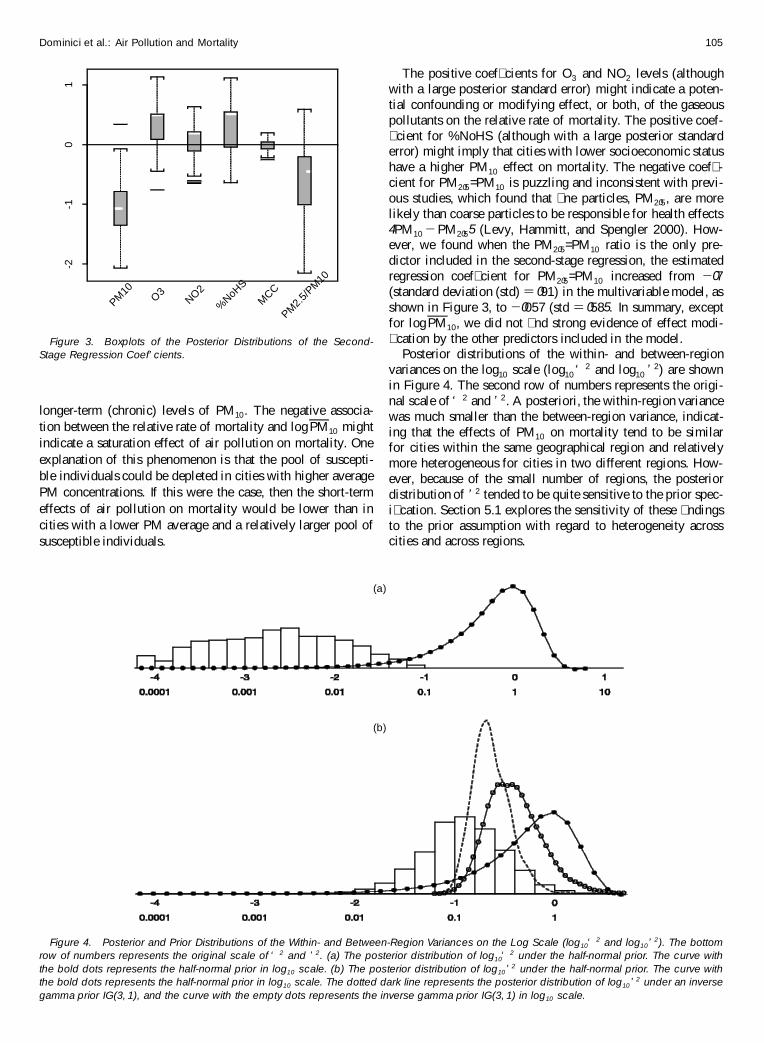
Figure 3 shows boxplots of the posterior distributions ofthe second-stage regression coef� cients Á. We found someevidence for modi� cation of the log-relative rate of mortal-ity associated with PM10 levels by logPM10 level in a direc-tion implying greater shorter-term (acute) effects at lower


-2-1

01

PM10

O3NO2

%NoHS

MCC

PM2.5

/PM

10

Figure 3. Boxplots of the Posterior Distributions of the Second-Stage Regression Coef’ cients.

longer-term (chronic) levels of PM10. The negative associa-tion between the relative rate of mortality and logPM10 mightindicate a saturation effect of air pollution on mortality. Oneexplanation of this phenomenon is that the pool of suscepti-ble individuals could be depleted in cities with higher averagePM concentrations. If this were the case, then the short-termeffects of air pollution on mortality would be lower than incities with a lower PM average and a relatively larger pool ofsusceptible individuals.

(a)

(b)

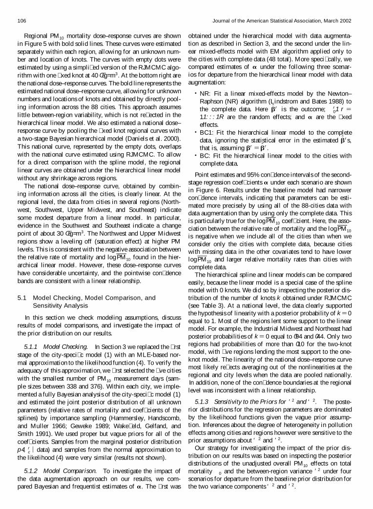
Figure 4. Posterior and Prior Distributions of the Within- and Between-Region Variances on the Log Scale (log10‘2 and log10’ 2). The bottom

row of numbers represents the original scale of ‘ 2 and ’ 2. (a) The posterior distribution of log10‘2 under the half-normal prior. The curve with

the bold dots represents the half-normal prior in log10 scale. (b) The posterior distribution of log10’2 under the half-normal prior. The curve withthe bold dots represents the half-normal prior in log10 scale. The dotted dark line represents the posterior distribution of log10’2 under an inversegamma prior IG(3, 1), and the curve with the empty dots represents the inverse gamma prior IG(3, 1) in log10 scale.

The positive coef� cients for O3 and NO2 levels (althoughwith a large posterior standard error) might indicate a poten-tial confounding or modifying effect, or both, of the gaseouspollutants on the relative rate of mortality. The positive coef-� cient for %NoHS (although with a large posterior standarderror) might imply that cities with lower socioeconomic statushave a higher PM10 effect on mortality. The negative coef� -cient for PM205=PM10 is puzzling and inconsistent with previ-ous studies, which found that � ne particles, PM205, are morelikely than coarse particles to be responsible for health effects4PM10 ƒ PM2055 (Levy, Hammitt, and Spengler 2000). How-ever, we found when the PM205=PM10 ratio is the only pre-dictor included in the second-stage regression, the estimatedregression coef� cient for PM205=PM10 increased from ƒ07(standard deviation (std) D 091) in the multivariable model, asshown in Figure 3, to ƒ0057 (std D 0585. In summary, exceptfor logPM10, we did not � nd strong evidence of effect modi-� cation by the other predictors included in the model.

Posterior distributions of the within- and between-regionvariances on the log10 scale (log10‘ 2 and log10 ’ 2) are shownin Figure 4. The second row of numbers represents the origi-nal scale of ‘ 2 and ’ 2. A posteriori, the within-region variancewas much smaller than the between-region variance, indicat-ing that the effects of PM10 on mortality tend to be similarfor cities within the same geographical region and relativelymore heterogeneous for cities in two different regions. How-ever, because of the small number of regions, the posteriordistribution of ’ 2 tended to be quite sensitive to the prior spec-i� cation. Section 5.1 explores the sensitivity of these � ndingsto the prior assumption with regard to heterogeneity acrosscities and across regions.


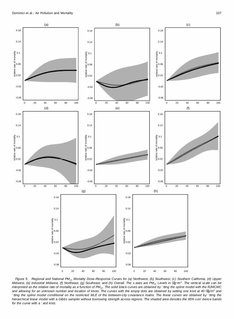
Regional PM10 mortality dose–response curves are shownin Figure 5 with bold solid lines. These curves were estimatedseparately within each region, allowing for an unknown num-ber and location of knots. The curves with empty dots wereestimated by using a simpli� ed version of the RJMCMC algo-rithm with one � xed knot at 40 Œg=m3. At the bottom right arethe national dose–response curves. The bold line represents theestimated national dose–response curve, allowing for unknownnumbers and locations of knots and obtained by directly pool-ing information across the 88 cities. This approach assumeslittle between-region variability, which is not re� ected in thehierarchical linear model. We also estimated a national dose–response curve by pooling the � xed knot regional curves witha two-stage Bayesian hierarchical model (Daniels et al. 2000).This national curve, represented by the empty dots, overlapswith the national curve estimated using RJMCMC. To allowfor a direct comparison with the spline model, the regionallinear curves are obtained under the hierarchical linear modelwithout any shrinkage across regions.

The national dose–response curve, obtained by combin-ing information across all the cities, is clearly linear. At theregional level, the data from cities in several regions (North-west, Southwest, Upper Midwest, and Southeast) indicatesome modest departure from a linear model. In particular,evidence in the Southwest and Southeast indicate a changepoint of about 30 Œg=m3. The Northwest and Upper Midwestregions show a leveling off (saturation effect) at higher PMlevels. This is consistent with the negative association betweenthe relative rate of mortality and logPM10 found in the hier-archical linear model. However, these dose–response curveshave considerable uncertainty, and the pointwise con� dencebands are consistent with a linear relationship.

5.1 Model Checking, Model Comparison, andSensitivity Analysis

In this section we check modeling assumptions, discussresults of model comparisons, and investigate the impact ofthe prior distribution on our results.

5.1.1 Model Checking. In Section 3 we replaced the � rststage of the city-speci� c model (1) with an MLE-based nor-mal approximation to the likelihood function (4). To verify theadequacy of this approximation, we � rst selected the � ve citieswith the smallest number of PM10 measurement days (sam-ple sizes between 338 and 376). Within each city, we imple-mented a fully Bayesian analysis of the city-speci� c model (1)and estimated the joint posterior distribution of all unknownparameters (relative rates of mortality and coef� cients of thesplines) by importance sampling (Hammersley, Handscomb,and Muller 1966; Geweke 1989; Wake� eld, Gelfand, andSmith 1991). We used proper but vague priors for all of thecoef� cients. Samples from the marginal posterior distributionp4‚r

c— data) and samples from the normal approximation to

the likelihood (4) were very similar (results not shown).

5.1.2 Model Comparison. To investigate the impact ofthe data augmentation approach on our results, we com-pared Bayesian and frequentist estimates of Á. The � rst was

obtained under the hierarchical model with data augmenta-tion as described in Section 3, and the second under the lin-ear mixed-effects model with EM algorithm applied only tothe cities with complete data (48 total). More speci� cally, wecompared estimates of Á under the following three scenar-ios for departure from the hierarchical linear model with dataaugmentation:

¡ NR: Fit a linear mixed-effects model by the Newton–Raphson (NR) algorithm (Lindstrom and Bates 1988) tothe complete data. Here OÂr is the outcome; � r

01 r D11 : : : 1 R are the random effects; and Á are the � xedeffects.

¡ BC1: Fit the hierarchical linear model to the completedata, ignoring the statistical error in the estimated OÂr s,that is, assuming Âr D OÂr .

¡ BC: Fit the hierarchical linear model to the cities withcomplete data.

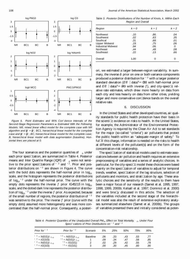
Point estimates and 95% con� dence intervals of the second-stage regression coef� cients Á under each scenario are shownin Figure 6. Results under the baseline model had narrowercon� dence intervals, indicating that parameters can be esti-mated more precisely by using all of the 88-cities data withdata augmentation than by using only the complete data. Thisis particularly true for the logPM10 coef� cient. Here, the asso-ciation between the relative rate of mortality and the logPM10

is negative when we include all of the cities than when weconsider only the cities with complete data, because citieswith missing data in the other covariates tend to have lowerlogPM10 and larger relative mortality rates than cities withcomplete data.

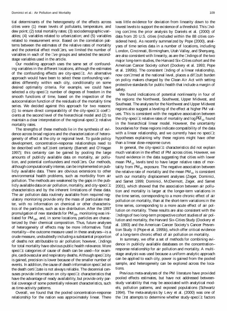
The hierarchical spline and linear models can be comparedeasily, because the linear model is a special case of the splinemodel with 0 knots. We did so by inspecting the posterior dis-tribution of the number of knots k obtained under RJMCMC(see Table 3). At a national level, the data clearly supportedthe hypothesis of linearity with a posterior probability of k D 0equal to 1. Most of the regions lent some support to the linearmodel. For example, the Industrial Midwest and Northeast hadposterior probabilities of k D 0 equal to 094 and 044. Only tworegions had probabilities of more than 010 for the two-knotmodel, with � ve regions lending the most support to the one-knot model. The linearity of the national dose–response curvemost likely re� ects averaging out of the nonlinearities at theregional and city levels when the data are pooled nationally.In addition, none of the con� dence boundaries at the regionallevel was inconsistent with a linear relationship.

5.1.3 Sensitivity to the Priors for ’ 2 and ‘ 2. The poste-rior distributions for the regression parameters are dominatedby the likelihood functions given the vague prior assump-tion. Inferences about the degree of heterogeneity in pollutioneffects among cities and regions however were sensitive to theprior assumptions about ‘ 2 and ’ 2.

Our strategy for investigating the impact of the prior dis-tribution on our results was based on inspecting the posteriordistributions of the unadjusted overall PM10 effects on totalmortality �0 and the between-region variance ’ 2 under fourscenarios for departure from the baseline prior distribution forthe two variance components ‘ 2 and ’ 2.

Dominici et al.: Air Pollution and Mortality 107re

lativ

e ra

te o

f mor

talit

y

-0.06

-0.02

0.02

0.06

0.1

0.14

0.18

0 20 40 60 80 100

oooooooooo

oooooooooo

oooooooooo

oooooooooooooo

oooooooooooooooooooooooooooooooooooooooooooooooooooooooo

rela

tive

rate

of m

orta

lity

-0.06

-0.02

0.02

0.06

0.1

0.14

0.18

0 20 40 60 80 100

oooooooooooooooooooooooooooooooooooooooooooooooooooooooooooooooooooooo

oooooooooooooo

oooooooooooo

oooo

rela

tive

rate

of m

ort

ality

-0.06

-0.02

0.02

0.06

0.1

0.14

0.18

0 20 40 60 80 100

oooooooo

oooooooo

oooooooo

oooooooo

oooooooooo

oooooooooooo

oooooooooooooo

ooooooooooooooooo

ooooooooooooooo

rela

tive

rate

of m

orta

lity

oooooooo

oooooooo

oooooooooo

oooooooooooooooooooooooooooooooooooooooooooooooooooooooooooooooooooooooooo

rela

tive

rate

of m

orta

lity

-0.06

-0.02

0.02

0.06

0.1

0.14

0.18

0 20 40 60 80 100

ooooooooooooooooooo

ooooooooooooooooooo

oooooooooooooooooooo


ooooooooooooooooooooo

ore

lativ

e ra

te o

f mor

talit

y

-0.06

-0.02

0.02

0.06

0.1

0.14

0.18

0 20 40 60 80 100

oooooo

ooooooo

ooooooo

ooooooo

ooooooo

oooooooo

oooooooo

oooooooo

oooooooo

oooooooo

oooooooo

oooooooo

oooooooo

oo

rela

tive

rate

of m

orta

lity

-0.06

-0.02

0.02

0.06

0.1

0.14

0.18

0 20 40 60 80 100

ooooooooooooooooooooooooooooooooooooooooooooooooooooo

oooooooooo

ooooooooo

oooooooo

oooooooo

ooooooo

ooooo

rela

tive

rate

of m

orta

lity

-0.06

-0.02

0.02

0.06

0.1

0.14

0.18

0 20 40 60 80 100

oooooooooooo

ooooooooooooo

ooooooooooooooo

ooooooooooooooooo


ooooooooooooooooooooooo

-0.06

-0.02

0.02

0.06

0.1

0.14

0.18

0 20 40 60 80 100

(h)(g)

(d) (e) (f)

(a) (b) (c)

Figure 5. Regional and National PM10 Mortality Dose–Response Curves for (a) Northwest, (b) Southwest, (c) Southern California, (d) UpperMidwest, (e) Industrial Midwest, (f) Northeast, (g) Southeast, and (h) Overall. The x-axes are PM10 Levels in Œg=m3 . The vertical scale can beinterpreted as the relative rate of mortality as a function of PM10. The solid black curves are obtained by ’ tting the spline model with the RJMCMCand allowing for an unknown number and location of knots. The curves with the empty dots are obtained by setting one knot at 40 Œg/m3 and’ tting the spline model conditional on the restricted MLE of the between-city covariance matrix. The linear curves are obtained by ’ tting thehierarchical linear model with a Gibbs sampler without borrowing strength across regions. The shaded area denotes the 95% con’ dence bandsfor the curve with a ’ xed knot.


NR BC1 BC B

log PM10

-3

-1.5

0

1.5

3

�

NR BC1 BC B

log O3

-3

-1.5

0

1.5

3

NR BC1 BC B

log NO2

-2

-1

0

1

2

NR BC1 BC B

log %NoHS

-2

-1

0

1

2

NR BC1 BC B

logit MCC

-1

-0.5

0

0.5

1

NR BC1 BC B

PM2.5/PM10

-4

-2

0

2

4

Figure 6. Point Estimates and 95% Con’ dence Intervals of theSecond-Stage Regression Parameters Á Estimated With the FollowingModels: NR, mixed linear effect model for the complete case with NRalgorithm and Âr D OÂr ; BC1, hierarchical linear model for the completecase and Âr D OÂr ; BC, hierarchical linear model for the complete case;B, hierarchical linear model with data augmentation (baseline). Hori-zontal lines are placed at 0.

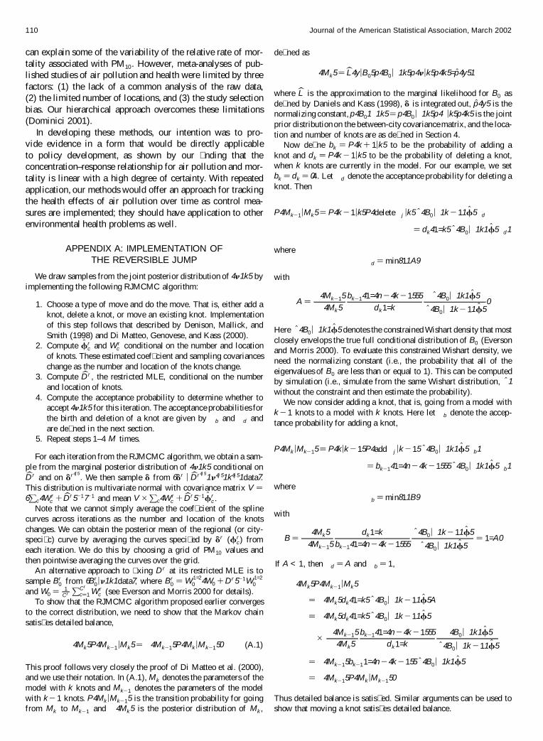
The four scenarios and the posterior quantiles of �0 undereach prior speci� cation, are summarized in Table 4. Posteriormeans and Inter Quartile Range ( IQR) of �0 were not sensi-tive to the prior speci� cations of ‘ 2 and ’2. Prior and pos-terior distributions on ’2 are shown in Figure 4. The curvewith the bold dots represents the half-normal prior in log10

scale, and the histogram represents the posterior distributionsof log10 ’ 2 under the half-normal prior. The curve with theempty dots represents the inverse ƒ prior IG431 15 in log10

scale, and the dotted dark line represents the posterior distribu-tion of log10 ’ 2 under the inverse ƒ prior. As expected, becauseof the small number of regions, the posterior distribution of ’ 2

was sensitive to the prior. The inverse ƒ prior (curve with theempty dots) assumed more heterogeneity and was more con-centrated than the half-normal prior. Consequently, a posteri-

Table 4. Posterior Quantiles of the Unadjusted Overall PM10 Effect on Total Mortality, �0 , Under FourSpeci’ cations of Prior Distributions on ‘ 2 and ’ 2

Prior for ‘ 2 Prior for ’2 Scenario 5% 25% 50% 75% 95%

‘ 2 N(011)I‘ 2>0 ’2 N(011)I’2>0 Baseline 006 033 043 053 077‘ 2 IG(313) ’2 N(011)I‘ 2 >0 1 009 034 047 058 085‘ 2 N(011)I‘ 2>0 ’2 IG(311) 2 002 029 042 055 078‘ 2 IG(313) ’2 IG(311) 3 000 030 045 060 090

Table 3. Posterior Distributions of the Number of Knots, k , Within EachRegion and Overall

Region k D 0 k D 1 k D 2

Northwest 010 086 004Southwest 002 063 035Southcal 031 068 001Upper Midwest 019 075 006Industrial Midwest 094 006 0Northeast 044 048 008Southeast 022 013 066

Overall 1000 0 0

ori, we estimated a larger between-region variability. In sum-mary, the inverse â prior on one or both variance componentsproduced a posterior distribution for ’ 2 with a larger posteriorstandard deviation (E6’ — data7 D 038 with half-normal priorand E6’ — data7 D 049 with inverse ƒ), and city-speci� c rel-ative rate estimates, which drew more heavily on data fromeach city and less heavily on data from other cities, yieldinglarger and more conservative con� dence bands on the overallrelative rate.

6. DISCUSSION

In the United States and other developed countries, air qual-ity standards for public health protection have their basis inthe scienti� c evidence on risks to health. In the United States,for example, the Administrator of the Environmental Protec-tion Agency is required by the Clean Air Act to set standardsfor the major (so-called “criteria”) air pollutants that protectthe public health within an “adequate margin of safety.” Toful� ll this charge, information is needed on the risks to healthat different levels of the pollutant(s) and on the form of theconcentration–risk relationship.

The speci� cation of statistical models used to estimate asso-ciations between air pollution and health requires an extensivepreprocessing of variables and a series of analytic choices. Inparticular, for the city-speci� c model these choices were basedmainly on the speci� cation of variables to adjust for temporaltrends, weather, speci� cation of the lag structure, selection ofpollutants and monitors, and strati� cation by age. These ana-lytic choices and the sensitivity of the results to them havebeen a major focus of our research (Samet et al. 1995, 1997,1998, 1999, 2000b; Kelsall et al. 1997; Dominici et al. 2000)and were brie� y discussed in this article. The selection ofthe variables included at the second stage of the hierarchi-cal model was also the result of extensive exploratory analy-ses summarized elsewhere (Samet et al. 2000b). The groupsof variables presented there and initially considered as poten-


tial determinants of the heterogeneity of the effects acrosscities were (1) mean levels of pollutants, temperature, anddew point; (2) total mortality rates; (3) sociodemographic vari-ables; (4) variables related to urbanization; and (5) variablesrelated to measurement error. Based on the correlation pat-terns between the estimates of the relative rates of mortalityand the potential effect modi� ers, we limited the number ofvariables in each of the � ve groups and selected the second-stage variables used in the article.

Our modeling approach uses the same set of confound-ing variables in the different locations, although the estimatesof the confounding effects are city-speci� c. An alternativeapproach would have been to select these confounding vari-ables differently within each city, conditionally on somedesired optimality criteria. For example, we could haveselected a city-speci� c number of degrees of freedom in thesmooth functions of time, based on the inspection of theautocorrelation function of the residuals of the mortality timeseries. We decided against this approach for two reasons:(1) to ensure direct comparability of the city-speci� c coef� -cients at the second level of the hierarchical model and (2) tomaintain a clear interpretation of the regional-speci� c relativemortality rates.

The strengths of these methods lie in the synthesis of evi-dence across broad regions and the characterization of hetero-geneity of effect at the city or regional level. To guide policydevelopment, concentration–response relationships need tobe described with suf� cient certainty (Barnett and O’Hagan1997); this certainty can be gained by pooling the largeamounts of publicly available data on mortality, air pollu-tion, and potential confounders and modi� ers. Our methods,although computationally intense, can be implemented on pub-licly available data. There are obvious extensions to otherenvironmental health problems, such as morbidity from airpollution. The methods are weakened by the gaps in the pub-licly available data on air pollution, mortality, and city-speci� ccharacteristics and by the inherent limitations of these data.The air pollution data routinely available from required reg-ulatory monitoring provide only the mass of particulate mat-ter, with no information on chemical or other characteris-tics of the particles, such as size distribution. After the 1997promulgation of new standards for PM205, monitoring was ini-tiated for PM205, and, in some locations, particles are charac-terized by their chemical composition. Thus, future analysesof heterogeneity of effects may be more informative. Totalmortality—the outcome measure used in these analyses—is acrude measure, undoubtedly including a substantial proportionof deaths not attributable to air pollution; however, � ndingsfor total mortality have obvious public health relevance. Morespeci� c categories of cause of death can be used—for exam-ple, cardiovascular and respiratory deaths. Although speci� cityis gained, precision is lower because of the smaller number ofevents. In addition, the cause of death information speci� ed onthe death certi� cate is not always reliable. The decennial cen-suses provide information on city-speci� c characteristics thathave the advantage of ready availability, but provide only par-tial coverage of some potentially relevant characteristics, suchas time-activity patterns.

Overall, we found that the pooled concentration–responserelationship for the nation was approximately linear. There

was little evidence for deviation from linearity down to thelowest levels to support the existence of a threshold. This � nd-ing con� rms the prior analysis by Daniels et al. (2000) ofdata from 20 U.S. cities (included within the 88 cities con-sidered here). As recently summarized by Pope (2000), anal-yses of time series data in a number of locations, includingLondon, Cincinnati, Birmingham, Utah Valley, and Shenyang,are also consistent with linearity, as are the � ndings of the twomajor long-term studies, the Harvard Six-Cities cohort and theAmerican Cancer Society cohort (Dockery et al. 1993; Popeet al. 1995b). The consistent � nding of a linear relationship,now con� rmed at the national level, places a dif� cult burdenon policy makers charged by the Clean Air Act with settingprotective standards for public health that include a margin ofsafety.

We found indications of potential nonlinearity in four ofthe regions: the Northwest, Southwest, Upper Midwest, andSoutheast. The analyses for the Northwest and Upper Midwestregions also suggest a leveling of the effect at higher PM val-ues. This is consistent with the negative association betweenthe city-speci� c relative rates of mortality and logPM10 foundin the hierarchical linear model. However, the uncertaintyboundaries for these regions indicate compatibility of the datawith a linear relationship, and we currently have no speci� chypotheses explaining why these regions might have otherthan a linear dose–response curve.

In general, the city-speci� c characteristics did not explainmuch variation in the effect of PM across cities. However, wefound evidence in the data suggesting that cities with lowermean PM10 levels tend to have larger relative rates of mor-tality from PM10 exposure. The negative association betweenthe relative rate of mortality and the mean PM10 is consistentwith our mortality displacement analyses (Zeger, Dominici,and Samet 1999; Dominici, McDermott, Zeger, and Samet2001), which showed that the association between air pollu-tion and mortality is larger at the longer-term variations inthe time series, corresponding to a more chronic effect of airpollution on mortality, than at the short-term variations in thetime series, corresponding to a more acute effect of air pol-lution on mortality. These results are also consistent with the� ndings of two long-term prospective cohort studies of air pol-lution and mortality, the Harvard Six-Cities Study (Dockery etal. 1993) and the American Cancer Society’s Cancer Preven-tion Study II (Pope et al. 1995b), which offer critical evidenceof a long-term chronic effect of air pollution on mortality.

In summary, we offer a set of methods for combining evi-dence in publicly available databases on the concentration–response relationship for air pollution and mortality. A multi-stage analysis was used because a uniform analytic approachcan be applied to each city, power is gained from the pooledsample, and heterogeneity can be explored across the loca-tions.

Previous meta-analyses of the PM literature have providedpooled effects estimates, but have not addressed between-study variability that may be associated with analytical mod-els, pollution patterns, and exposed populations (Schwartz1994). The meta-analysis by Levy et al. (2000) was one ofthe � rst attempts to determine whether study-speci� c factors


can explain some of the variability of the relative rate of mor-tality associated with PM10. However, meta-analyses of pub-lished studies of air pollution and health were limited by threefactors: (1) the lack of a common analysis of the raw data,(2) the limited number of locations, and (3) the study selectionbias. Our hierarchical approach overcomes these limitations(Dominici 2001).

In developing these methods, our intention was to pro-vide evidence in a form that would be directly applicableto policy development, as shown by our � nding that theconcentration–response relationship for air pollution and mor-tality is linear with a high degree of certainty. With repeatedapplication, our methods would offer an approach for trackingthe health effects of air pollution over time as control mea-sures are implemented; they should have application to otherenvironmental health problems as well.

APPENDIX A: IMPLEMENTATION OFTHE REVERSIBLE JUMP

We draw samples from the joint posterior distribution of 4Í1 k5 byimplementing the following RJMCMC algorithm:

1. Choose a type of move and do the move. That is, either add aknot, delete a knot, or move an existing knot. Implementationof this step follows that described by Denison, Mallick, andSmith (1998) and Di Matteo, Genovese, and Kass (2000).

2. Compute OÔrc and W r

c conditional on the number and locationof knots. These estimated coef� cient and sampling covarianceschange as the number and location of the knots change.

3. Compute bDr , the restricted MLE, conditional on the numberand location of knots.

4. Compute the acceptance probability to determine whether toaccept 4Í1 k5 for this iteration. The acceptance probabilities forthe birth and deletion of a knot are given by �b and �d andare de� ned in the next section.

5. Repeat steps 1–4 M times.

For each iteration from the RJMCMC algorithm, we obtain a sam-ple from the marginal posterior distribution of 4Í1 k5 conditional onbDr and on Är 4j5

. We then sample Ä from 6Är — bDr 4j51Í4j51 k4j51data7.

This distribution is multivariate normal with covariance matrix V D6P

c4W rc

C bDr 5ƒ17ƒ1 and mean V � Pc4W

rc

C bDr 5ƒ1 OÔrc .

Note that we cannot simply average the coef� cient of the splinecurves across iterations as the number and location of the knotschanges. We can obtain the posterior mean of the regional (or city-speci� c) curve by averaging the curves speci� ed by Är (Ôr

c) fromeach iteration. We do this by choosing a grid of PM10 values andthen pointwise averaging the curves over the grid.

An alternative approach to � xing Dr at its restricted MLE is tosample Br

0 from 6Br0—Í1 k1 data7, where Br

0D W 1=2

0 4W0 C Dr 5ƒ1W 1=20

and W0 D 1Cr

PCr

cD1 W rc (see Everson and Morris 2000 for details).

To show that the RJMCMC algorithm proposed earlier convergesto the correct distribution, we need to show that the Markov chainsatis� es detailed balance,

� 4Mk5P4Mkƒ1—Mk5 D � 4Mkƒ15P4Mk—Mkƒ150 (A.1)

This proof follows very closely the proof of Di Matteo et al. (2000),and we use their notation. In (A.1), Mk denotes the parameters of themodel with k knots and Mkƒ1 denotes the parameters of the modelwith k ƒ 1 knots. P4Mk—Mkƒ15 is the transition probability for goingfrom Mk to Mkƒ1 and � 4Mk5 is the posterior distribution of Mk ,

de� ned as

� 4Mk5 D bL4y—B05p4B0—�1k5p4Í—k5p4k5= Op4y51

where bL is the approximation to the marginal likelihood for B0 asde� ned by Daniels and Kass (1998), Ä is integrated out, Op4y5 is thenormalizing constant, p4B01 �1 k5 D p4B0—�1 k5p4�—k5p4k5 is the jointprior distribution on the between-city covariance matrix, and the loca-tion and number of knots are as de� ned in Section 4.

Now de� ne bkD P4k C 1—k5 to be the probability of adding a

knot and dk D P4k ƒ 1—k5 to be the probability of deleting a knot,when k knots are currently in the model. For our example, we setbk

D dkD 04. Let �d denote the acceptance probability for deleting a

knot. Then

P4Mkƒ1—Mk5 D P4k ƒ1—k5P4delete �j —k5 O� 4B0—�1k ƒ 11 OÔ5�d

D dk41=k5 O� 4B0—�1k1 OÔ5�d1

where�d D min811 A9

with

A D � 4Mkƒ15

� 4Mk5

bkƒ141=4nƒ 4k ƒ1555

dk1=k

O� 4B0—�1k1 OÔ5

O� 4B0—�1 k ƒ 11 OÔ50

Here O� 4B0—�1 k1 OÔ5 denotes the constrained Wishart density that mostclosely envelops the true full conditional distribution of B0 (Eversonand Morris 2000). To evaluate this constrained Wishart density, weneed the normalizing constant (i.e., the probability that all of theeigenvalues of B0 are less than or equal to 1). This can be computedby simulation (i.e., simulate from the same Wishart distribution, O� 1

without the constraint and then estimate the probability).We now consider adding a knot, that is, going from a model with

k ƒ 1 knots to a model with k knots. Here let �b denote the accep-tance probability for adding a knot,

P4Mk—Mkƒ15 D P4k—k ƒ15P4add �j —k ƒ15 O� 4B0—�1k1 OÔ5�b1

D bkƒ141=4nƒ 4k ƒ1555 O� 4B0—�1k1 OÔ5�b1

where�b D min811B9

with

B D � 4Mk5

� 4Mkƒ15

dk1=k

bkƒ141=4nƒ 4k ƒ1555

O� 4B0—�1 k ƒ 11 OÔ5

O� 4B0—�1 k1 OÔ5D 1=A0

If A < 1, then �d D A and �b D 1,

� 4Mk5P4Mkƒ1—Mk5

D � 4Mk5dk41=k5 O� 4B0—�1k ƒ11 OÔ5A

D � 4Mk5dk41=k5 O� 4B0—�1k ƒ11 OÔ5

� � 4Mkƒ15

� 4Mk5

bkƒ141=4nƒ 4k ƒ1555

dk1=k

� 4B0—�1k1 OÔ5

O� 4B0—�1k ƒ11 OÔ5

D � 4Mkƒ15bkƒ11=4nƒ 4k ƒ155 O� 4B0—�1k1 OÔ5

D � 4Mkƒ15P4Mk—Mkƒ150

Thus detailed balance is satis� ed. Similar arguments can be used toshow that moving a knot satis� es detailed balance.


If instead of sampling B0, we � x it at its restricted MLE, bB0 (bD),then the foregoing argument proceeds similarly. However, the productof the prior for B0 and the likelihood approximation, bL4y—B05, in� 4Mk5 is now replaced by bL4y—bB04bD55. In addition, the transition andacceptance probabilities remain the same, except for the exclusionof O� 4B0—Í1 k1 OÔ5. The approach of � xing D at its restricted MLEestimate simpli� es computations. However, it decreases the size ofthe penalty for models with more knots (see Di Matteo et al. 2000).

[Received December 2000. Revised August 2001.]

REFERENCES

American Thoracic Society, and Bascom, R. (1996a), “Health Effects of Out-door Air Pollution,” Part 1, American Journal of Respiratory and CriticalCare Medicine, 153, 3–50.

(1996b), “Health Effects of Outdoor Air Pollution,” Part 2, AmericanJournal of Respiratory and Critical Care Medicine, 153, 477–498.

Barnett, V., and O’Hagan, A. (1997), Setting Environmental Standards: TheStatistical Approach to Handling Uncertainity and Variation, New York:Chapman and Hall.

Best, N. G., Cowles, M. K., and Vines, K. (1995), “CODA: ConvergenceDiagnostics and Output Analysis Software for Gibbs Sampling Output,”Technical Report, Version 0.30, University of Cambridge, MRC Biostatis-tics Unit.

Daniels, M., Dominici, F., Samet, J. M., and Zeger, S. L. (2000), “EstimatingPM10-Mortality Dose-Response Curves and Threshold Levels: An Analysisof Daily Time-Series for the 20 Largest U.S. Cities,” American Journal ofEpidemiology, 152, 397–412.

Denison, D., Mallick, B., and Smith, A. (1998), “Automatic Bayesian CurveFitting,” Journal of the Royal Statistical Society, Ser. B, 60, 333–350.

Di Matteo, I., Genovese, C., and Kass, R. (to appear), “Bayesian Curve FittingWith Free-Knot Splines,” technical report, Carnegie Mellon University.

Dockery, D., Pope, C. A., Xu, X., Spengler, J., Ware, J., Fay, M., Ferris, B.,and Speizer, F. (1993), “An Association Between Air Pollution and Mortal-ity in Six U.S. Cities,” New England Journal of Medicine, 329, 1753–1759.

Dominici, F. (in press), “Air Pollution and Health: What can we Learn froman Hierarchical Approach?” Invited Commentary, American Journal of Epi-demiology, 155, 1–5.

Dominici, F., McDermott, A., Zeger, S. L., and Samet, J. M. (2001), “AirborneParticulate Matter and Mortality: Time-scale Effects in Four U.S. Cities,”American Journal of Epidemiology, .

Dominici, F., Samet, J. M., and Zeger, S. L. (2000), “Combining Evidenceon Air Pollution and Daily Mortality From the Twenty Largest U.S. Cities:A Hierarchical Modeling Strategy” (with discussion), Journal of the RoyalStatistical Society, Ser. A, 163, 263–302.

Environmental Protection Agency (1996), “Review of the National AmbientAir Quality Standards for Particulate Matter: Policy Assessment of Scien-ti� c and Technical Information,” OAQPS Staff Paper.

Everson, P., and Morris, C. (2000), “Inference for Multivariate Normal Hier-archical Models,” Journal of the Royal Statistical Society, Ser. B, 62,399–412.

Gelfand, A. E., and Smith, A. F. M. (1990), “Sampling-Based Approaches toCalculating Marginal Densities,” Journal of the American Statistical Asso-ciation, 85, 398–409.

Gelman, A., and Rubin, D. B. (1992), “Inference From Iterative Simula-tion Using Multiple Sequences” (with discussion), Statistical Science, 7,457–472.

Geweke, J. (1989), “Bayesian Inference in Econometric Models Using MonteCarlo Integration,” Econometrica, 57, 1317–1339.

Gilks, W. R., Richardson, S., and Spiegelhalter, D. J. (eds.) (1996), MarkovChain Monte Carlo in Practice, London: Chapman and Hall.

Hammersley, J. M., Handscomb, D. C. A., and Muller, M. E. R. (1966),“Review of Monte Carlo Methods,” The Annals of Mathematical Statistics,37, 532–538.

Hastie, T. J., and Tibshirani, R. J. (1990), Generalized Additive Models, NewYork: Chapman and Hall.

Kelsall, J., Samet, J. M., and Zeger, S. L. (1997), “Air Pollution and Mortal-ity in Philadelphia, 1974–1988,” American Journal of Epidemiology, 146,750–762.

Levy, J., Hammitt, J., and Spengler, J. (2000), “Estimating the MortalityImpacts of Particulate Matter: What Can be Learned From Between-StudyVariability?,” Environmental Health Perspectives, 108, 109–117.

Lindstrom, M. J., and Bates, D. M. (1988), “Newton–Raphson and EM Algo-rithms for Linear Mixed-Effects Models for Repeated-Measures Data,”Journal of the American Statistical Association, 83, 1014–1022.

Pauler, D., and Wake� eld, J. (2000), “Modeling and Implementation Issues inBayesian Meta-Analysis,” in Meta-Analysis in Medicine and Health Policy,pp. 231–254, New York: Marcel Dekker.

Pope, C. A. (2000), “Invited Commentary: Particulate Matter-MortalityExposure-Response Relations and Threshold,” American Journal of Epi-demiology, 152, 407–412.

Pope, C. A., Dockery, D., and Schwartz, J. (1995a), “Review of Epidemio-logical Evidence of Health Effects of Particulate Air Pollution,” InhalationToxicology, 47, 1–18.

Pope, C. A., Thun, M., Namboodiri, M., Dockery, D., Evans, J., Speizer, F.,and Heath, C. (1995b), “Particulate Air Pollution as a Predictor of Mortalityin a Prospective Study of U.S. Adults,” American Journal of Respiratory aCritical Care Medicine, 151, 669–674.

Raftery, A., and Lewis, S. (1992), “How Many Iterations in the Gibbs Sam-pler?,” in Bayesian Statistics 4, Proceedings of the Fourth Valencia Inter-national Meeting, pp. 763–774.

Samet, J. M., Dominici, F., Curriero, F., Coursac, I., and Zeger, S. L.(2000a), “Fine Particulate Air Pollution and Mortality in 20 US Cities:1987–1994” (with discussion), New England Journal of Medicine, 343,1742–1757.

Samet, J. M., Zeger, S. L., and Berhane, K. (1995), The Association of Mortal-ity and Particulate Air Pollution, Cambridge, MA: Health Effects Institute.

Samet, J. M., Zeger, S. L., Dominici, F., Curriero, F., Coursac, I., Dockery, D.,Schwartz, J., and Zanobetti, A. (2000b), The National Morbidity, Mortality,and Air Pollution Study (HEI Project No. 96-7): Morbidity and Mortalityfrom Air Pollution in the United States, Cambridge, MA: Health EffectsInstitute.

Samet, J. M., Zeger, S. L., Dominici, F., Dockery, D., and Schwartz, J. (1999),The National Morbidity, Mortality, and Air Pollution Study (HEI ProjectNo. 96-7): Methods and Methodological Issues, Cambridge, MA: HealthEffects Institute.

Samet, J. M., Zerger, S. L., Kelsall, J. E., Xu and Kalkstein, L. (1998), “DoesWeather Confound or Modify the Association of Particulate Air Pollutionwith Mortality?” Environmental Research, 77, 9–19.

Samet, J. M., Zeger, S. L., Kelsall, J., Xu, J., and Kalkstein, L. (1997), “AirPollution, Weather and Mortality in Philadelphia,” in Particulate Air Pollu-tion and Daily Mortality: Analyses of the Effects of Weather and MultipleAir Pollutants, The Phase IB report of the Particle Epidemiology Evalua-tion Project, Cambridge, MA: Health Effects Institute.

Schwartz, J. (1994), “Air Pollution and Daily Mortality: A Review and MetaAnalysis,” Environmental Research, 64, 36–52.

Tanner, M. A. (1991), Tools for Statistical Inference—Observed Data andData Augmentation Methods, Lecture Notes in Statistics, Vol. 67, NewYork: Springer-Verlag.

Wake� eld, J. C., Gelfand, A. E., and Smith, A. F. M. (1991), “Ef� cient Gen-eration of Random Variates via the Ratio-of-Uniforms Method,” Statisticsand Computing, 1, 129–133.

Zeger, S. L., Dominici, F., and Samet, J. M. (1999), “Harvesting-ResistantEstimates of Pollution Effects on Mortality,” Epidemiology, 89, 171–175.

Air Pollution and Mortality: Estimating Regional and ... · Air Pollution and Mortality: Estimating...

Documents

Transcript of Air Pollution and Mortality: Estimating Regional and ... · Air Pollution and Mortality: Estimating...