Air Jets for Lift Control in LowReynolds Number Flow

by

Erik Skensved

A thesispresented to the University of Waterloo

in fulfilment of thethesis requirement for the degree of

Master of Applied Sciencein

Mechanical Engineering

Waterloo, Ontario, Canada, 2010

c© Erik Skensved 2010

I hereby declare that I am the sole author of this thesis. This is a true copy of thethesis, including any required final revisions, as accepted by my examiners.

I understand that my thesis may be made electronically available to the public.

iii

Abstract

The environmental and monetary cost of energy has renewed interest in horizontal-axis wind turbines (HAWT). One problem with HAWT design is turbulent winds,which cause cyclic loading and reduced life. Controlling short-term aerodynamicfluctuations with blade pitching or mechanical flaps is limited by the speed of ac-tuation. The objective was to investigate using jet-flap-like fluidic actuators onthe ‘suction surface’ of an aerofoil for rapid aerodynamic control. A NACA 0025aerofoil was constructed for wind-tunnel experiments. The low Reynolds number(Re) flow was measured non-intrusively with particle image velocimetry (PIV). Thejet showed limited effect compared to published work. The sharp trailing edge anddistance to the jet were determined to be critical factors. At Re ≈ 100000 the‘suction surface’ jet sheet is less useful for control than the conventional ‘pressuresurface’ sheet. The experiment suggests usage near the blade root on truncatedaerofoils.

v

Acknowledgements

I would like to thank Dr. David Johnson for supervision and guidance of this re-search, as well as his assistance with the preparation of this document. I would alsolike to thank Stephen Orlando for assistance with the Laser Doppler Anemometer,and also for taking the photographs which appear in this report. Thanks also toBrian Gaunt and Michel McWilliam for advice on the Particle Image Velocimetrymethod.

vii

Dedication

This thesis is dedicated to my parents.Without them none of this would be possible.

ix

Contents

List of Tables xv

List of Figures xviii

Nomenclature xix

1 Introduction 1

2 Literature Review 3

2.1 Dynamic Stall . . . . . . . . . . . . . . . . . . . . . . . . . . . . . . 3

2.2 The Jet Flap . . . . . . . . . . . . . . . . . . . . . . . . . . . . . . 5

2.2.1 Introduction to the Jet Flap . . . . . . . . . . . . . . . . . . 5

2.2.2 Additional Information About the Jet Flap . . . . . . . . . . 9

2.3 Related Work . . . . . . . . . . . . . . . . . . . . . . . . . . . . . . 14

2.3.1 Numerical Study Comparing a Circulation Control Rotor toa Gurney Flap Equipped Rotor . . . . . . . . . . . . . . . . 14

2.3.2 Experimental Comparison of a Gurney Flap and a Jet Flap . 17

2.3.3 Experimental Comparison of Discrete Translating Micro-tabsto a Solid Gurney Flap . . . . . . . . . . . . . . . . . . . . . 18

2.3.4 Numerical Simulation of Lift Control Using a CurvedMechanical Flap . . . . . . . . . . . . . . . . . . . . . . . . 19

3 Experimental Model 21

3.1 Pattern and Mold . . . . . . . . . . . . . . . . . . . . . . . . . . . . 22

3.2 Models . . . . . . . . . . . . . . . . . . . . . . . . . . . . . . . . . . 23

3.3 Model Air Supply . . . . . . . . . . . . . . . . . . . . . . . . . . . . 24

xi

4 Jet Flow Study Setup 27

4.1 Particle Seeding . . . . . . . . . . . . . . . . . . . . . . . . . . . . . 27

4.2 LDA Probe Details . . . . . . . . . . . . . . . . . . . . . . . . . . . 29

5 Jet Flow Validation 33

5.1 Jet Velocity Profile . . . . . . . . . . . . . . . . . . . . . . . . . . . 33

5.2 Span-wise Jet Flow Uniformity . . . . . . . . . . . . . . . . . . . . 34

5.3 Jet Momentum Integration . . . . . . . . . . . . . . . . . . . . . . . 40

5.4 Jet Momentum Comparison . . . . . . . . . . . . . . . . . . . . . . 42

6 Particle Image Velocimetry Experiment 47

6.1 Aerofoil Setup . . . . . . . . . . . . . . . . . . . . . . . . . . . . . . 47

6.2 Light Sheet Setup . . . . . . . . . . . . . . . . . . . . . . . . . . . . 48

6.3 Camera and Data Acquisition System Setup . . . . . . . . . . . . . 49

6.4 Experimental Cases . . . . . . . . . . . . . . . . . . . . . . . . . . . 49

6.5 Data Collection . . . . . . . . . . . . . . . . . . . . . . . . . . . . . 51

7 PIV Data Processing 53

7.1 PIV Cross-correlation . . . . . . . . . . . . . . . . . . . . . . . . . . 53

7.2 Correction of the Flow . . . . . . . . . . . . . . . . . . . . . . . . . 57

7.3 Lift and Drag Calculation . . . . . . . . . . . . . . . . . . . . . . . 58

7.4 Error Propagation . . . . . . . . . . . . . . . . . . . . . . . . . . . 59

8 PIV Data Pooling 61

9 Lift Control Results 73

9.1 Low Speed Results . . . . . . . . . . . . . . . . . . . . . . . . . . . 73

9.2 High Speed Results . . . . . . . . . . . . . . . . . . . . . . . . . . . 73

9.3 Comparison with Prior Work . . . . . . . . . . . . . . . . . . . . . 74

9.3.1 Zero Momentum Flux Data . . . . . . . . . . . . . . . . . . 75

9.3.2 Zero Angle of Attack Data . . . . . . . . . . . . . . . . . . . 76

9.4 Pressure Lift . . . . . . . . . . . . . . . . . . . . . . . . . . . . . . . 78

9.5 Pressure Lift Replacement . . . . . . . . . . . . . . . . . . . . . . . 81

xii

10 Conclusions and Recommendations 85

10.1 Conclusions . . . . . . . . . . . . . . . . . . . . . . . . . . . . . . . 85

10.2 Recommendations . . . . . . . . . . . . . . . . . . . . . . . . . . . . 86

References 86

APPENDICES 91

A Ancillary Information on Jet Experiment 93

A.1 Beam Properties . . . . . . . . . . . . . . . . . . . . . . . . . . . . 93

A.2 Jet Momentum Integration Uncertainty . . . . . . . . . . . . . . . . 94

A.3 LDA Data Rate . . . . . . . . . . . . . . . . . . . . . . . . . . . . . 95

A.4 Measured Jet Properties . . . . . . . . . . . . . . . . . . . . . . . . 96

A.5 Equation of Two Dimensional Jet Profile . . . . . . . . . . . . . . . 97

A.6 Momentum Integral . . . . . . . . . . . . . . . . . . . . . . . . . . . 97

B Ancillary Information on Lift Control Experiment 99

B.1 Measured Angle of Attack in PIV Experiment . . . . . . . . . . . . 99

B.2 Wake Profiles from PIV Experiment . . . . . . . . . . . . . . . . . . 100

xiii

List of Tables

2.1 Summary of Std(N) reduction . . . . . . . . . . . . . . . . . . . . . 20

4.1 Dimensions of the probe volumes . . . . . . . . . . . . . . . . . . . 29

5.1 Full span centre line survey . . . . . . . . . . . . . . . . . . . . . . 34

5.2 Full span grid survey . . . . . . . . . . . . . . . . . . . . . . . . . . 38

5.3 Comparison between velocity and standard deviation . . . . . . . . 40

5.4 Momentum integrated over cross-section . . . . . . . . . . . . . . . 41

5.5 Average jet width . . . . . . . . . . . . . . . . . . . . . . . . . . . . 42

8.1 Summary of cases . . . . . . . . . . . . . . . . . . . . . . . . . . . . 61

8.2 Summary of data . . . . . . . . . . . . . . . . . . . . . . . . . . . . 61

A.1 LDA beam properties . . . . . . . . . . . . . . . . . . . . . . . . . . 93

A.2 Jet half width at 10× 10−3 m . . . . . . . . . . . . . . . . . . . . . 96

A.3 Jet half width at 15× 10−3 m . . . . . . . . . . . . . . . . . . . . . 96

A.4 Pressure with flow rate . . . . . . . . . . . . . . . . . . . . . . . . . 96

B.1 Measured α at low Re . . . . . . . . . . . . . . . . . . . . . . . . . 99

B.2 Measured α at high Re . . . . . . . . . . . . . . . . . . . . . . . . . 99

xv

List of Figures

2.1 Schematic of stall response with sinusoidal LFA . . . . . . . . . . . 4

2.2 Basic mechanism of the jet flap . . . . . . . . . . . . . . . . . . . . 8

2.3 Lift vs. momentum flux curve from Dimmock . . . . . . . . . . . . 11

2.4 Surface pressure profiles from Dimmock . . . . . . . . . . . . . . . . 12

2.5 Trailing-edge surface pressure discontinuity from Dimmock . . . . . 13

2.6 Jet drag coefficient from Dimmock . . . . . . . . . . . . . . . . . . 15

3.1 Half-profile pattern and mold . . . . . . . . . . . . . . . . . . . . . 22

3.2 Schematic of in-wing air distribution manifold . . . . . . . . . . . . 23

3.3 Dimensions of the aerofoil . . . . . . . . . . . . . . . . . . . . . . . 24

3.4 Model trailing edge . . . . . . . . . . . . . . . . . . . . . . . . . . . 25

3.5 Model air supply . . . . . . . . . . . . . . . . . . . . . . . . . . . . 25

4.1 Model mounted in test section . . . . . . . . . . . . . . . . . . . . . 28

4.2 Schematic of LDA measurement plane . . . . . . . . . . . . . . . . 28

4.3 LDA probe geometry . . . . . . . . . . . . . . . . . . . . . . . . . . 30

5.1 Local coordinate system . . . . . . . . . . . . . . . . . . . . . . . . 34

5.2 Velocity field . . . . . . . . . . . . . . . . . . . . . . . . . . . . . . 35

5.3 Velocity components . . . . . . . . . . . . . . . . . . . . . . . . . . 36

5.4 Full span flow field . . . . . . . . . . . . . . . . . . . . . . . . . . . 37

5.5 Repeated jet geometry . . . . . . . . . . . . . . . . . . . . . . . . . 38

5.6 Average jet . . . . . . . . . . . . . . . . . . . . . . . . . . . . . . . 39

5.7 Standard deviation of velocity . . . . . . . . . . . . . . . . . . . . . 39

5.8 Gaussian curve overlaid on jet data . . . . . . . . . . . . . . . . . . 43

5.9 Momentum comparison between LDA and the isentropic assumption 44

5.10 Comparison between data and curve fit at maximum m . . . . . . . 45

xvii

6.1 Angle and force sign conventions . . . . . . . . . . . . . . . . . . . 47

6.2 Schematic of double light sheet . . . . . . . . . . . . . . . . . . . . 48

6.3 Side view of optical layout . . . . . . . . . . . . . . . . . . . . . . . 49

6.4 Top view of PIV setup . . . . . . . . . . . . . . . . . . . . . . . . . 50

7.1 Raw image example . . . . . . . . . . . . . . . . . . . . . . . . . . . 54

7.2 Schematic of single light sheet . . . . . . . . . . . . . . . . . . . . . 55

7.3 Example of an exported ensemble-averaged flow field . . . . . . . . 56

7.4 Aerofoil mirror images . . . . . . . . . . . . . . . . . . . . . . . . . 57

8.1 Comparison between first and second ensemble . . . . . . . . . . . . 63

8.2 Pooled ensemble pairs at α = 0◦ . . . . . . . . . . . . . . . . . . . . 64

8.3 Pooled ensemble pairs at α = 5◦ . . . . . . . . . . . . . . . . . . . . 65

8.4 Pooled ensemble pairs at α = 10◦ . . . . . . . . . . . . . . . . . . . 67

8.5 Recirculating flow in replicate 2 . . . . . . . . . . . . . . . . . . . . 68

8.6 Pooled ensemble pairs at α = 15◦ . . . . . . . . . . . . . . . . . . . 69

8.7 Comparison of wake profiles at 10◦ and Re = 0.120× 106 (replicate 1) 70

8.8 Comparison of wake profiles at 10◦ and Re = 0.120× 106 (replicate 2) 70

8.9 Comparison of wake profiles at 10◦ and Re = 0.120× 106 (replicate 3) 71

9.1 Pooled Cl versus Cµ curves at low Re . . . . . . . . . . . . . . . . . 74

9.2 Pooled Cl versus Cµ curves at high Re . . . . . . . . . . . . . . . . 75

9.3 Comparison of lift experiment with Sandia National Laboratories data 76

9.4 Comparison between zero angle of attack results and typical jet-flapexperiment . . . . . . . . . . . . . . . . . . . . . . . . . . . . . . . . 77

9.5 Effect of tripping the boundary layer . . . . . . . . . . . . . . . . . 78

9.6 Low speed flow wake profiles for 0◦ and 5◦ . . . . . . . . . . . . . . 79

9.7 Low speed flow wake profiles for 10◦ and 15◦ . . . . . . . . . . . . . 80

9.8 Flow visualization of the trailing edge separation . . . . . . . . . . . 81

9.9 Experimental Cl with ‘replaced’ pressure lift (0◦ and 5◦) . . . . . . 83

9.10 Experimental Cl with ‘replaced’ pressure lift (10◦ and 15◦) . . . . . 84

A.1 LDA data rate . . . . . . . . . . . . . . . . . . . . . . . . . . . . . . 95

B.1 High speed flow wake profiles for 0◦ and 5◦ . . . . . . . . . . . . . . 100

B.2 High speed flow wake profiles for 10◦ and 15◦ . . . . . . . . . . . . . 101

xviii

Nomenclature

Roman Symbols

∆t Time interval between PIV frames [s]

∆X Particle shift between PIV frames [m]

m Mass flow rate per unit span [kg s−1 m−1]

Aj Area of the fluid jet [m2]

c Blade or aerofoil chord [m]

Cµ Jet momentum coefficient

Cl Lift coefficient

ClCµ=0 Lift coefficient with jet off

ClCµ6=0Lift coefficient with jet on

Cl,measured Measured lift coefficient

d Diameter of jet holes [m]

ds Beam separation distance [m]

f Focal length [m]

h Wind tunnel height [m]

l Distance along laser beam from waist [m]

pf Flow pressure [Pa]

r Span location [m]

Rair Specific gas constant for air [J kg−1 K−1]

s Jet-flapped span [m]

Std(N) Standard deviation of the normal force on blade [N]

xix

t Overall aerofoil half-thickness as a fraction of c

Tf Flow temperature [K]

U∞ Free-stream velocity [m s−1]

Vj Speed of the fluid jet [m s−1]

Vx,y,n Time averaged local jet velocity [m s−1]

w Beam half width [m]

x, y, z Local tunnel coordinates [m]

yt Local aerofoil half-thickness as a fraction of c

V x,y Average local jet velocity over all jets [m s−1]

C Jet supply loss coefficient

Re Reynolds number

X,Y,Z Global tunnel coordinates [m]

Greek Symbols

α Angle of attack [rad]

λ Wavelength of light [m]

ω Angular velocity [rad s−1]

φ LDA beam intersection angle [rad]

ρ∞ Free stream density [kg m−3]

ρj Density of the fluid jet [kg m−3]

σx,y Local standard deviation of velocity [m s−1]

θ Jet deflection angle ≡ angle between zero-lift lineand the jet direction at the trailing edge [rad]

ξ Dummy coordinate for chord-wise position (0 < ξ < 1)

Subscripts

0 Beam waist

des Indicates design conditions

f Focal distance from waist

xx

Chapter 1

Introduction

In the modern world, one of the key resources is energy; this fact is self evident.With concerns over the price of fossil fuels, and their environmental impact, interestin wind as a source of energy has been renewed [1]. Historically wind was capturedin order to deliver mechanical power for a particular task. The current use ofhorizontal-axis wind turbines (HAWT) to generate electricity is the focus of thisdocument.

Briefly, horizontal-axis wind turbines, described more thoroughly by Burton etal. [1], consist of one or more aerofoil-shaped blades attached to a horizontallymounted shaft. The action of the wind on the blades creates the shaft torquenecessary to turn an electrical generator either directly or through a gearbox. Theblade-shaft-generator system is mounted on a vertical-axis yaw assembly and eitherpivots freely, or is actively oriented, into the wind. The designer of such a windturbine is concerned with its ability to generate power safely over its design lifetime.A contributing factor to both the safety and lifespan of a turbine is the ability tocontrol its operation within prescribed limits.

One of the key problems with wind turbine design is that, in operation, turbinesare subject to unpredictable wind conditions. Design of turbines using the bladeelement method (BEM) assuming uniform constant wind is relatively well known.Unfortunately such conditions do not exist in nature. Variations in wind can becategorized as long-term or short-term and as periodic or random.

Control of turbines experiencing long-term uniform fluctuations has been achievedwith variable-slip generators, variable-pitch blades, and by coupling the generatorto the grid through special power electronics [1]. Control of short-term variationswith these traditional methods is limited due to practical pitching rates and rotorinertia.

Periodic short-term fluctuations are those that occur ‘N-times per revolution’.For example vertical wind shear or error in the turbine orientation (yaw error)causes a periodic change in both the angle and magnitude of the flow over the bladeas it rotates. This of course leads to a periodic load being applied to the blades

1

and accordingly the whole turbine. Though it has been proposed that turbineblades could be cyclically pitched [1] [2] the practicality is questionable due torequired pitching rates. It has been suggested that the decrease in rotor speedwith increasing diameter could lead to cyclic pitch being more practical, howeverincreasing the blade size may also reduce achievable pitching rates.

Random velocity fluctuations result from natural turbulence in the wind. The-oretically, independent blade pitching could be implemented, but different radiallocations would require different magnitudes of pitch change. Thus even this solu-tion would require a compromise over the blade span.

The final consideration of short-term variations is that dynamic effects cannotbe neglected. In particular the variation of aerofoil lift that is associated with dy-namic stall cannot be neglected. This change in lift from expected levels affects themechanical forces on the turbine components and is a strong incentive to attemptcontrol of short-term variation.

The main objective of this research is to investigate the potential of using high-velocity air jets to control the response of aerofoils in low to moderate Reynoldsnumber (Re) flow. Specifically the objective is to use a jet flap on the ‘suctionsurface’ of an orthodox aerofoil to reduce the lift and drag forces similar to anaileron.

Chapter 2 below is devoted to a brief review of: literature on the dynamic stallphenomena, prior work on jet flaps, and other related work on aerodynamic control.In Chapter 3 the construction of the aerofoil model that was used in the wind-tunnel experiments is described along with its air supply system. Chapters 4 and 5detail the setup and analysis of the laser Doppler anemometer (LDA) measurementsused to validate the control jet. In Chapters 6, 7, 8, and 9 the main wind-tunnelexperiment is detailed. The basic particle image velocimetry (PIV) setup used fordata collection is reviewed in Chapter 6. The calculations performed to extractresults from the raw data is described in Chapters 7 and 8. Chapter 9 presentsthe lift control results from the PIV experiment along with comparison data fromprevious work. Finally in Chapter 10 the conclusions and recommendations of theresearch are summarized.

2

Chapter 2

Literature Review

The purpose of this chapter is to provide a general overview of relevant literatureon the topic of aerodynamic flow control as it relates to wind turbines. Morespecifically the goal is to highlight what research has been done and what has yetto be done. Finally the reviewed literature provides a basis that is built upon inthe current work.

2.1 Dynamic Stall

Static stall of an aerofoil can be considered a steady process. The unsteady coun-terpart to static stall is dynamic stall. Dynamic stall occurs when the timescale ofthe stall process is of equal or smaller order to the fluid-mechanic timescale [3].

An experiment was conducted by Schreck and Robinson [4] to investigate thedynamic stall response of HAWT blades. This dynamic stall condition leads toamplified fluctuating loads, which shorten machine life and may cause variations inthe voltage or phase of the generated power. According to the authors the inabilityto mitigate dynamic stall phenomena in turbine designs results from an inabilityto produce a detailed aerodynamic model. This itself is a result of ignorance ofthe fundamental three-dimensional flow fields about dynamically-stalling turbineblades. Another contributing factor, not mentioned by the authors, is the inabilityto provide an adequate control response to dynamic stall.

In previous two-dimensional wind-tunnel experiments [3] it was found that whenan aerofoil is rapidly pitched beyond the static stall angle a small, energetic vortex isformed near the leading edge. This vortex grows and convects downstream over theaerofoil suction surface causing a temporary low surface pressure and accordinglyhigh lift. Once the vortex convects off the surface the aerofoil is statically stalled.Even in this simplified case there exist complex vortex kinematics. To extendunderstanding to the flow kinematics of operating HAWTs, the full rotating casemust be investigated.

3

The rotational case was studied using the Unsteady Aerodynamics Experiment(UAE) upwind turbine in the NASA Ames wind tunnel [5]. One of the two bladeswas outfitted with surface pressure taps. Local flow angle (LFA) was measured withfive-hole probes on 0.8c long stalks attached to the leading edge of the blade. Thesestalks were offset from the surface pressure taps, but one might question whetherthey could disturb the flow, particularly if it were already unstable. Ideally anoninvasive measurement method should be used.

The UAE turbine was set at yaw angles from 10◦ to 60◦ during the experiments.A nonzero yaw angle causes the HAWT blades to experience pseudo-sinusoidal vari-ations in angle of attack (α) and LFA with azimuthal angle. Under this conditionthe blade α can rise above the static stall limit during its rotation. The LFA re-sults from the vector addition of the tunnel free-stream velocity (U∞) and the localazimuthal velocity (r · ω). The authors note that the LFA was used directly andnot converted to α due to uncertainty over how the flow angle changes between theposition of the five-hole probe and the leading edge of the aerofoil.

The dynamic stall vortex was detected by the passage of a local minima insurface pressure by the rows of pressure taps. Since there was good repeatabil-ity between the 36 blade-rotation cycles, the data from the cycles were ensembleaveraged into a single pressure profile for each condition.

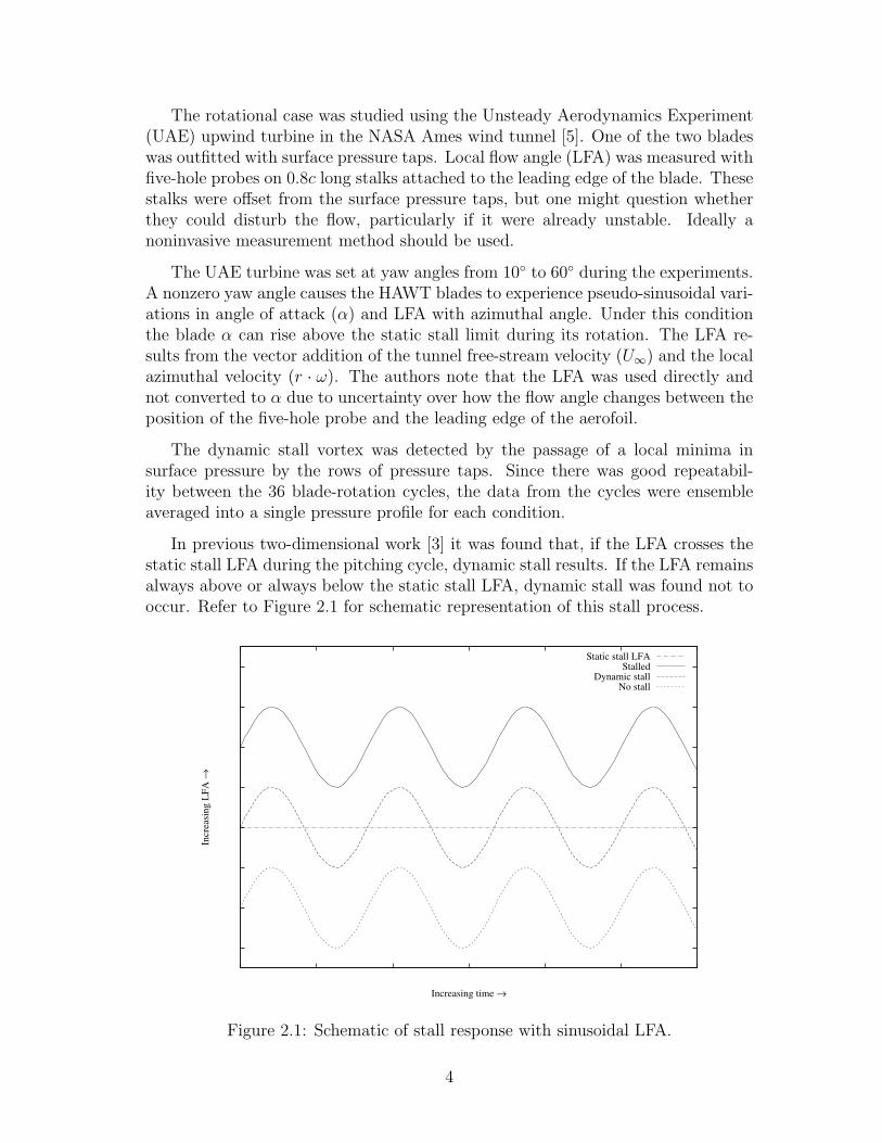
In previous two-dimensional work [3] it was found that, if the LFA crosses thestatic stall LFA during the pitching cycle, dynamic stall results. If the LFA remainsalways above or always below the static stall LFA, dynamic stall was found not tooccur. Refer to Figure 2.1 for schematic representation of this stall process.

Incr

easi

ng L

FA

→

Increasing time →

Static stall LFAStalled

Dynamic stallNo stall

Figure 2.1: Schematic of stall response with sinusoidal LFA.

4

In this three-dimensional study it was found that, though dynamic stall willnot occur if the static stall limit is not crossed, dynamic stall may not occur evenif the limit is crossed. Similarly if the LFA always exceeds the stall limit, thenone would expect that the aerofoil would remain statically stalled. This is alsonot necessarily the case in three-dimensional flow. This limit crossing rule gives ageneral guideline as to when three-dimensional flow will dynamically stall, howeverit must be realized that it is not an accurate predictor.

It was found that, the LFA at which dynamic stall initiated, was dependenton the radial location on the blade. The inboard position initiated at the lowestangle followed closely by the outboard section. Interestingly, the midsection of theblade was most resistant to dynamic stall initiation. Though the midsection wasthe last region to initiate stall, the vortex convection rate was higher than thatof the root or tip. The authors suggest that the stall vortex was pinned, which isto say convection was impeded, at the root and tip of the blade, hence its overallconvection rate was slowed and it was not released off the blade.

As either U∞ or the yaw angle were increased the dynamic stall vortex extendedfrom the root towards the tip. No evidence of the vortex reaching the blade tip wasfound. This leads to the conclusion that attempts to mitigate the dynamic stallevent should be focused on the region from the mid-span to near, but not directlyat, the blade root.

2.2 The Jet Flap

The purpose of this section is to provide some background into the jet flap andprior analytical and experimental work done by other researchers. The first work isa general overview of the pioneering work, both analytical and experimental, on thejet flap. The second paper details a single set of early work done by Dimmock [6].

2.2.1 Introduction to the Jet Flap

A survey of the important experimental and theoretical work on the jet flap up untilabout 1960 was done by Korbacher and Sridhar [7]. The purpose was to aggregatewhat was known and highlight what was not known.

The ‘jet flap’ is an aerodynamic flow control device that is analogous to thetraditional mechanical flap. As implied by the name, this device uses a jet of airto control air flowing over an aerofoil. This flow control affects both the air of theboundary layer, near the aerofoil surface, and the circulation of the air far from thesurface.

The distinction between boundary layer control (BLC) and circulation control(CC) is not well defined. Generally BLC refers to either: blowing air to increasethe momentum of the air flow near the surface of the aerofoil, or suction to remove

5

this low-momentum air. The purpose of controlling the boundary layer is typicallyto prevent the flow from separating from the aerofoil surface. There are also othertechniques that have been investigated to energize the flow, however they are notdescribed herein. Circulation control picks up where BLC leaves off. The goal istypically to increase the circulation above the ‘natural’ level of an aerofoil with fullyattached flow.

The use of the term ‘jet flap’ is broad and encompasses both the ‘blown flap’ andits variations, as well as the ‘pure jet flap’ that does not involve a physical surface.The blown flap, in the context of CC, involves the use of a small flap or shroudedflap to redirect a high speed jet of fluid, via the Coanda effect [8], at an angle θ tothe chord of the aerofoil. The high-momentum fluid increases the effective size ofthe small movable flap. In contrast the pure jet flap consists of a high-momentumjet of fluid exhausted directly from a nozzle, movable or not, without the physicalflap surface, so that the jet of fluid itself acts as the flap.

For low momentum jets theoretical work has shown that the blown flap is moreeffective than the pure variety. The experiments presented in Chapters 4 and6 are concerned with a configuration more similar to the pure flap for practicalconsiderations. For this reason research related to the pure flap is the focus of thischapter.

Two key hypotheses were proposed; the lift hypothesis and the thrust hypothe-sis. These hypotheses rely on three assumptions: no mixing between the jet and thesurrounding fluid, no profile drag, and two-dimensional flow with no induced drag.Under these conditions the jet, beginning at an angle θ to the free stream, mustcurve and asymptotically approach the direction of the free stream. If the jet—astreamline—does not eventually reach the free stream direction it would impart aninfinite momentum in the vertical direction to the flow field.

Thrust hypothesis: The jet thrust experienced by the aerofoil in the counterstream wise direction is equal to the magnitude of the jetthrust at the outlet regardless of the initial angle (θ) ofthe jet [7].

Lift hypothesis: The total lift of the jet flapped aerofoil is equal to the pres-sure lift exerted on the aerofoil and its imaginary solidcurved flap plus the reaction component of the jet in thelifting direction [7].

There are several different rigorous arguments, not described here, for both ofthese hypothesis. Of course real air flow is not two-dimensional nor ideal, hencethese predictions are somewhat optimistic. Nevertheless the indicated potential forlift and thrust enhancement are still enticing.

The jet momentum coefficient (Equation 2.1) is the non-dimensional parametermost frequently used to characterize the jet in BLC and CC research. In essence it isa ratio of the jet momentum flux (jet thrust) over pressure force (dynamic pressuremultiplied by area). The coefficient used throughout this document utilizes the

6

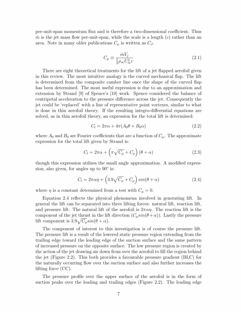
per-unit-span momentum flux and is therefore a two-dimensional coefficient. Thusm is the jet mass flow per-unit-span, while the scale is a length (c) rather than anarea. Note in many older publications Cµ is written as CJ .

Cµ ≡mVj

12ρ∞U2

∞c(2.1)

There are eight theoretical treatments for the lift of a jet flapped aerofoil givenin this review. The most intuitive analogy is the curved mechanical flap. The liftis determined from the composite camber line once the shape of the curved flaphas been determined. The most useful expression is due to an approximation andextension by Strand [9] of Spence’s [10] work. Spence considered the balance ofcentripetal acceleration to the pressure difference across the jet. Consequently thejet could be ‘replaced’ with a line of representative point vortexes, similar to whatis done in thin aerofoil theory. If the resulting integro-differential equations aresolved, as in thin aerofoil theory, an expression for the total lift is determined:

Cl = 2πα + 4π(A0θ + B0α) (2.2)

where A0 and B0 are Fourier coefficients that are a function of Cµ. The approximateexpression for the total lift given by Strand is:

Cl = 2πα +(π√

Cµ + Cµ

)(θ + α) (2.3)

though this expression utilizes the small angle approximation. A modified expres-sion, also given, for angles up to 90◦ is:

Cl = 2παη +(3.9√

Cµ + Cµ

)sin(θ + α) (2.4)

where η is a constant determined from a test with Cµ = 0.

Equation 2.4 reflects the physical phenomena involved in generating lift. Ingeneral the lift can be separated into three lifting forces: natural lift, reaction lift,and pressure lift. The natural lift of the aerofoil is 2παη. The reaction lift is thecomponent of the jet thrust in the lift direction (Cµsin(θ+α)). Lastly the pressurelift component is 3.9

√Cµsin(θ + α).

The component of interest to this investigation is of course the pressure lift.The pressure lift is a result of the lowered static pressure region extending from thetrailing edge toward the leading edge of the suction surface and the same patternof increased pressure on the opposite surface. The low pressure region is created bythe action of the jet drawing air down from over the aerofoil to fill the region behindthe jet (Figure 2.2). This both provides a favourable pressure gradient (BLC) forthe naturally occurring flow over the suction surface and also further increases thelifting force (CC).

The pressure profile over the upper surface of the aerofoil is in the form ofsuction peaks over the leading and trailing edges (Figure 2.2). The leading edge

7

air drawndown by jet

pressure peaks

suction peaks

jet sheet

upstreameffect

Figure 2.2: Basic mechanism of the jet flap.

suction peak is responsible for the net thrust being independent of θ, as stated in thethrust hypothesis. In non-ideal flow the leading edge suction peak is diminishedwith respect to the trailing edge peak. This is particularly true if leading edgeseparation occurs and can lead to negative net thrust being generated (net drag).Larger leading edge radii tend to create pressure gradients more favourable forattached flow in this region.

As the angle of attack of the aerofoil increases a separation bubble forms nearthe leading edge. The action of the jet causes the leading edge separated flow toreattach. The jet behaves somewhat like an ejector pump strongly drawing theupstream flow over the aerofoil. The size of the separation bubble can increase byextending until it reaches the trailing edge.

Stall of a jet flapped aerofoil occurs when the separation bubble bursts open andforms a wake. This is caused by either an increase in α or θ such that the influenceof the jet can no longer maintain flow attachment. Thus the stall α decreases withincreased θ. It is therefore important to be cautious with setting θ to avoid flowseparation.

Not surprisingly the other parameter that plays a role in flow separation andstall, in addition to α and θ, is the Reynolds number. The Reynolds number of thejet flapped aerofoil is based on the chord of the aerofoil, the free stream velocityand the kinematic viscosity of the air (Re = U∞c

ν). The Reynolds number has

been found to have a large effect on the lift and drag of the jet flapped aerofoil.Korbacher and Sridhar [7] state that while a Re of 4× 106 may approximate cruiseconditions in aircraft (20 × 106), an approximation of slow flight Re = 5 × 106

by a Reynolds number of 1× 106 could be problematic due to laminar separation.Korbacher and Sridhar refer to the work of Dimmock [6] on the effects of Reynoldsnumber. This research is described in Section 2.2.2 below.

8

Experimental evidence [11] shows that the measured thrust is less than thethrust predicted by the thrust hypothesis, which is equal to the total jet momen-tum flux. This being said the thrust at large θ is greater than the pure reactioncomponent of the jet, lending support to the hypothesis. Part of this deficit can beattributed to the non-ideal mixing that is contrary to the basic assumptions. It hasbeen found that the entrainment angle of the flow into the jet can be over 90◦. Inidealized flow the jet is a streamline and the external flow is parallel. Even in ideal-ized jet mixing the flow is also parallel not perpendicular, so in the real case therewill be some ‘secondary losses’ [11] beyond the primary mixing loss. Another issuein jet mixing is entrainment of the slow moving boundary layer. Since entrainmentrate is proportional to the difference in velocity between the streams [12] the jetspreading rate is increased by the boundary layer and the entrainment occurs at alarger angle incurring higher losses. In addition to loss of thrust in the entrainmentprocess the reduced pressure in the trailing edge region contributes to overall dragon the aerofoil.

The relation of Korbacher and Sridhar’s jet flap review to the current workshould be clear. Knowledge of the general working principle of the flap is key to itsuse. The lift and thrust hypotheses suggest it is possible to use a jet flap to controlthe lift force on the blade while at the same time recovering power through the shafttorque created by the jet thrust. Non-ideal effects were revealed through Korbacherand Sridhar’s experimentation. These effects are responsible for diminishing theeffect of the jet and so care is required to create an effective system.

2.2.2 Additional Information About the Jet Flap

The following work done by Dimmock [6] was done with a view at using full-span propulsive jets in aeronautical applications namely aircraft wings. This basicresearch allowed the testing of the theoretical predictions of aerodynamic forcesand moments, particularly the lift and thrust hypotheses.

The aerofoil chosen was an elliptical section 12.5% thick with a 0.203 m chordand a 0.305 m span. This very low aspect ratio leads to doubt about the two-dimensionality of the flow. An ellipse was chosen for ease of comparison betweenexperiments and analytic predictions that require coordinate transformations. Itwas thought that an elliptical section might be as appropriate as any other aerofoilsection for a jet flapped wing. This section does not have the sharp trailing edgecommon to most low speed aerofoils, hence its performance with the jet turnedoff is not the same as conventional sections. Three jet deflection angles (θ) of 0◦,31.4◦, 90◦ were tested by fabricating the aerofoil with a replaceable brass trailingedge. The latter two angles allowed the effect of θ to be studied, while the 0◦ anglewas used to isolate the drag due to jet entrainment. The model was suspended atboth ends of the span by the parallel arms of a thrust balance. Lift was determinedfrom 26 static pressure taps situated around the aerofoil section. The model wassupplied with compressed air for the jet.

9

Reynolds Number Effects

The Reynolds number used in Dimmock’s experiment was the chordal value asdefined in Section 2.2.1. Due to the limited tunnel size the aerofoil chord couldnot be made large enough to test at full scale Reynolds number. In the 90◦ modeltests the Re ranged from 0.425× 106 to 0.459× 106 for 0.000 ≤ Cµ ≤ 0.467. In the31.4◦ model tests the Re was 0.425 × 106 for Cµ ≤ 0.50 and from 0.147 × 106 to0.425× 106 for 0.50 < Cµ ≤ 4.17.

As a result of the generally low and variable Reynolds number in the experimentssome care must be taken in interpreting the results. Three factors lead Dimmockto conclude that flow transition was occurring: an abrupt change in slope of the liftversus momentum flux curve (Figure 2.3), the appearance of a trailing edge suctionpeak at roughly the same Cµ (Figure 2.4), and also a discontinuity in the surface-pressure curve near the trailing edge (Figure 2.5). Consequently experiments weredone with trip wires in various locations on the chord to determine the effect oftransition and separation. Experiments were done with trip wires installed at bothleading and trailing edges of the suction and pressure surfaces. The final positionof the trip wires on both surfaces was at 82% of chord near the trailing edge.

Further experimentation was done with smoke and wool tufts. This demon-strated that momentum deficiency in the boundary layer, which normally formsa wake, absorbed jet momentum. Decreased available jet momentum results indecreased lift augmentation and decreased net thrust. The presence of the tripwires caused the boundary layer to be tripped and re-energized, thereby prevent-ing flow separation and net momentum loss. Dimmock suggested that the loss ofmomentum due to laminar separation near the trailing edge is greater than thatof a turbulent boundary layer. In other words a thick boundary layer causes loss,however a separated boundary layer causes more loss.

If the jet momentum, and therefore the lift coefficient, is increased beyond alimit the flow transitions from laminar to turbulent near the leading edge. Afterthis point the trailing edge trip wire has no effect. The slope of the lift versusmomentum curve lowers slightly at this point revealing the loss in effective jetstrength.

At higher jet momentum flux, and higher lift, the flow separates near the leadingedge. Despite the separation, the lift continued to increase smoothly and the trailingedge suction peak continued to increase.

It was noted that there was separation evident at the trailing edge with the90◦ jet always. It seems reasonable that, independent of the Reynolds number, thetrailing edge configuration may affect the separation behaviour of the aerofoil.

Entrainment Effects

In addition to the aforementioned loss in effective jet strength when thick or sep-arated boundary layers are entrained into the jet there is also the manner of the

10

Figure 2.3: Lift versus momentum flux curve from Dimmock [6]. Test conditions:α = 0◦ and θ = 90◦. Note change in slope at approximately Cµ = 0.04 indicatingtransition. Note also that CJ ≡ Cµ.

11

Figure 2.4: Surface pressure profiles from Dimmock [6]. Note existence of trailing-edge suction peak in (d) and (e), but not in (a), (b), or (c). Note also that CJ ≡ Cµ.

12

Figure 2.5: Surface pressure profile from Dimmock [6]. Note the discontinuity inthe pressure trace near 100% of chord. Note also that CJ ≡ Cµ.

13

entrainment. Again experimentation with wool tufts and smoke revealed that theflow was turned perpendicular to the jet before being entrained. In the ideal caseno mixing occurs. Ideal jet mixing involves parallel streams. The basic assumptionsare not consistent with parallel mixing and so there is a loss.

Using the 90◦ model the thrust was measured first with the pressure distribution,then later with the thrust balance. Though the maximum measured thrust wasonly 37% of the raw jet momentum flux, this still provides support for the thrusthypothesis, since the direct component of thrust is zero. When Cµ exceeded 0.4 theflow separated at the leading edge and there was a reduction in measured thrust.

The entrained flow around the aerofoil can influence the pressure distribution.If the pressure in the vicinity of the jet is lowered there will be an increase in thedrag force; this is termed ‘jet drag’. Experimentation with a 0◦ trailing edge jetallowed this drag component to be measured (Figure 2.6). It was found that, in thisimplementation, the jet drag was approximately 0.06Cµ for Cµ < 0.10 and 0.017Cµ

at higher values of Cµ (Re = 0.425× 106). At Re = 0.212× 106 the slope continuesat 0.06 until Cµ = 0.25 then changes to 0.0104. It may be that these values varydepending on implementation, however this does give an order of magnitude of thejet drag loss.

2.3 Related Work

The purpose of this section is to review the prior research into the use of trailing-edge devices for active lift control on wind turbine blades. This was done with aview of using control jets to influence the net circulation around the blade section.Emphasis has been given to the Gurney flap as it is somewhat analogous to thelow-momentum jet flap. Though not directly applicable, such related studies canlend valuable ideas to the current body of research.

2.3.1 Numerical Study Comparing a Circulation ControlRotor to a Gurney Flap Equipped Rotor

A numerical study of the flow around the National Renewable Energy Laboratory(NREL) Phase VI rotor was completed by Tongchitpakdee et al. [13]. The studycompared the use of a fixed Gurney flap and a trailing-edge Coanda jet at low andhigh wind speeds. The NREL Phase VI rotor uses stall-controlled S809 blades.Since stall-controlled machines can only operate in a very limited range of windspeeds, there is an incentive to increase the power extracted under low wind-speedconditions.

The circulation control technology used by Tongchitpakdee et al. [13] is similarto that found in other studies. The basic premise is that a high-momentum jet offluid is ejected tangential to a curved surface. As long as the pressure differential

14

Figure 2.6: Jet drag coefficient from Dimmock [6]. All symbols except x’s are fromtests at Re = 0.425× 106. Note also that CJ ≡ Cµ.

15

across the jet is sufficient to balance the centripetal acceleration the fluid will followthe surface. This is the so called ‘Coanda Effect’. In this case the S809 aerofoilwas modified to have a small jet slot at 93% of chord on the suction surface and arounded trailing edge. To minimize the drag penalty associated with a blunt trailingedge only the upper surface was curved, while the lower surface was maintained flat.In other studies a corner between upper and lower surfaces is avoided, since thisessentially fixes the location of the rear stagnation point. The jet flow thereforecauses only the front stagnation point to move backward along the lower aerofoilsurface. Significant turning of the inviscid outer flow is still achieved.

Gurney flaps are also devices used to change the circulation, and hence the lift,of an aerofoil. In this study small tabs were placed at the trailing edge of thepressure surface. These tabs extended 0.015c into the flow from the rotor surface.

This study used unsteady compressible Reynolds-averaged Navier-Stokes (RaNS)equations in three dimensions. The Reynolds number of the rotor tip in this inves-tigation was 1.3× 106.

The key results of the study are as follows. The Coanda jet was effective atincreasing both the lift and thrust at low wind speed (7 m s−1). The Gurney flapwas also able to increase the circulation of the blade, however with this methodthere was a drag penalty.

At high speed (15 m s−1) the flow separated from the upper surface of the rotorwith both methods. Neither method was able to augment the thrust or normalforce of the rotor significantly, but only increase the drag on the rotor. The authorssuggest that a leading-edge jet may be able to suppress leading-edge separation andallow the trailing-edge jet to be effective.

In this paper the authors introduce a potentially useful concept of excess power(Equation 2.5). The excess power represents the benefit of using the lift enhance-ment technology. The cost in terms of power consumed can also be representedas a percentage of the baseline power. The suggested expression for cost is Equa-tion 2.6, where C is a coefficient to account for the inefficiencies of the jet supplysystem. Obviously if the excess power is greater than the power consumed then thecirculation-control method is worthwhile.

Excess Power ≡

Power generated bycirculation control rotor

− Power from thebaseline configuration

Power from the baseline configuration× 100%

(2.5)

Power Consumed ≡ 1

2CρjAjV

3j (2.6)

16

2.3.2 Experimental Comparison of a Gurney Flap and a JetFlap

Another study, relevant to the current research, was the experimental work doneby Traub et al. [14]. This study was a comparison between a trailing-edge jet flapand a Gurney flap. The central idea of this study was the ability to control theflow, or ‘virtually alter’ the aerofoil profile, without conventional moving parts. Inthe words of the authors “hingeless flow control.” This has the stated advantageof: stealth, reduced weight, compactness, increased robustness and increased tol-erance of damage. All but the first stated advantage are relevant to wind turbinetechnology.

The model used in the experiment was a NACA 0015 aerofoil fitted with endplates to ensure two-dimensional flow. The aerofoil dimensions were 0.71 m chordand 0.235 m span, thus the aspect ratio was a rather low one-third. The aerofoilwas constructed with a 1×10−3 m jet slot located 15×10−3 m from the trailing edgeor 98% of chord. The jet deflection angle (θ) was 90◦. For comparison, data werealso acquired with a 0.0075c Gurney-flap attached to the aerofoil at the location ofthe jet slot. The Reynolds number was 0.7× 106 and turbulence intensity was lessthan 0.5%. A three-component force balance was used to measure forces.

The authors present some of the more interesting results in terms of ‘lift-augmentation ratio’. This is defined in Equation (2.7) and essentially comparesthe lift increment to the momentum supplied. If this ratio is greater than one, thenthe change in lift is larger than the reactive (thrust) component of the jet.

ClCµ6=0− ClCµ=0

Cµ

(2.7)

The authors found that, not surprisingly, the jet-flap shifts the Cl - α curveupwards increasing the lift for a given α similar to a conventional flap. It wasdetermined that the lift-augmentation ratio is approximately 15 to 5 for 0.0037 ≤Cµ ≤ 0.029. The key finding here is that the ratio decreases with increasing Cµ,but is still significantly larger than one. Another key finding is that a Cµ of 0.0068causes the same lift increment as the 0.0075c height Gurney flap in the same locationin this implementation.

It was determined that at low α the Gurney flap had a small drag penalty, sincethe combination of jet power plus jet-flap drag is smaller than the Gurney-flap drag.At higher α the drag of the Gurney flap decreases and the aforementioned trendreverses.

On surface flow visualization was done using a thin plate, attached parallel tothe end plates, with a titanium dioxide and kerosene mixture applied to it. Theresulting streaks gave a qualitative idea of the flow behaviour. The authors concludethat, though the Cl may be the same, the flow is different around the Gurney andjet flaps. The key difference is that, while the Gurney-flap deflects the flow and

17

creates a wake, the jet-flap absorbs the free stream and actually draws the flowaround the sharp trailing edge.

A serious criticism of this work is the very low aspect-ratio model used. Thoughend plates were used to maintain two-dimensional flow the authors admit that theplates were not large enough. Given the strong aspect-ratio effect noted in otherjet-flap research [7], the magnitudes of the lift increments are questionable.

The key fact brought to light in this study is that the lift-augmentation ratiodecreases with increasing momentum. Furthermore the relation developed analyt-ically by Spence (Cl ∝

√Cµ) [15] was found to model the diminishing returns in

lift. The final key finding was that the flow was drawn down around the sharptrailing edge and that the jet essentially becomes the dividing streamline.

2.3.3 Experimental Comparison of Discrete TranslatingMicro-tabs to a Solid Gurney Flap

An experimental and computational comparison of discrete translating tabs, as op-posed to hinged tabs, with solid Gurney flaps was done by Nakafuji et al. [16]. Themotivation for this work was the lack of fast acting control mechanisms currentlyavailable to mitigate wind turbine blade loads. The authors propose the use ofmicro-electro-mechanical (MEM) translational tabs for trailing edge control. Thestated advantage of these MEM devices is their low cost and light weight, as wellas being appropriate for installation in a small trailing edge. The proposed methodof use is in an on-off capacity, wherein the on state functions similar to a Gurneyflap.

In order to optimize size and location of the tab devices a two-dimensionalRaNS computational fluid dynamic (CFD) study was done on a GU25-5(11)-8aerofoil. This aerofoil was chosen for its similarity to typical thick wind turbineblade sections. The CFD and wind-tunnel lift results agree well with previouslypublished results up to approximately 8◦. At higher angles the stall behaviour ofthe three results deviated significantly, the experiment having a higher stall angleand the computation having a lower maximum Cl. Thus computational results thatinclude separated flow should, not surprisingly, be treated with caution.

In the CFD study the tab position was varied between 0c and 0.10c in distancefrom the trailing edge. It was found that the Cl increased with tab position between0c and 0.02c, and decreased slightly from that point to 0.10c. In the experimentalstudy the Cl was high at 0c and decreased slightly from that point to 0.10c. In otherwords the experiment did not show the initial increase that the CFD showed. Thisbrings to light the fact that, for Gurney flaps at least, it is unnecessary to place theflap directly at the trailing edge. The computation showed that the drag decreasedfrom 0c to 0.02c and increased from there to 0.10c. Experimental results for dragwere not presented due to excessive uncertainty, which is a common problem. Againit must be remembered that the flow behind the flap is badly separated and it istherefore worth questioning the accuracy of the computations.

18

The effect of tab height was also studied. The lift coefficient increased with tabheights between 0.0025c and 0.02c. The incremental improvement with tab heighthowever was a decreasing trend, so the overall lift coefficient was limited. Thecomputational Cl results generally agreed with the experimental Cl results. Thecomputational drag results showed a sharp drop from 0c to 0.0025c in height andan increase from there to 0.02c in height.

The authors conclude that, if the internal volume of the aerofoil is consideredalong with the Cl and Cd results, the best compromise is to mount the flap at 95%of chord or 0.05c from the trailing edge.

The aforementioned results are for two-dimensional flow over a continuous flap.For practical application the individual tabs require a small gap between them. Theeffect of different gap spacings, as a fraction of tab height, was also investigated.The spacing/height ratios used were: 0.5, 1, and 2. With the solid tab the liftenhancement was approximately 50%, while with the 0.5 ratio it was 42%. Withthe largest ratio the enhancement dropped to 20%. The important fact to noticehere is that, so long as the spacing is not large, discrete tabs are almost as effectiveas solid flaps. It was also noted by the authors that discontinuous flaps have somedrag reduction benefits, so the optimal configuration may not be the one with themaximum lift. Though such a fact cannot be applied directly to jet flaps, it doessuggest the possibility of using discontinuous blowing slots.

2.3.4 Numerical Simulation of Lift Control Using a CurvedMechanical Flap

A numerical aeroelastic study of an aerofoil with an actively controlled flap hasbeen conducted by Buhl et al. [17]. Based on previous work, the authors state thatthere is significant potential for the reduction of wind turbine blade loads by usingan active control scheme. The study corresponds to a rather large hypothetical10 MW pitch regulated wind turbine with a hypothetical 6 s rotational period.

An aerodynamic model for unsteady two-dimensional potential flow over a thinaerofoil with a deflecting camber line was used in this study. Using this model topredict lift forces is suitable so long as separation does not occur. The chosen aero-foil used was the Risø B1-18 with a cubic spline superimposed on the trailing 10%to form a curved flap. In this study the aerofoil was modelled as a rigid mass sus-pended in the two-dimensional plane on x, y, and rotational spring/dampers. Twobase cases were investigated: a step in wind velocity and turbulence superimposedon average wind velocity.

The aerodynamic model was validated against a RaNS code. It was found thatthis code was able to predict the steady forces on the aerofoil for flap deflectionangles of ±10◦ and attached flow. It was however found that the code overestimatedthe dynamic amplitude of the forces by 50%, although the dynamic response wasotherwise correct. According to the authors this is adequate for the purpose of

19

variable trailing edge testing, but the accuracy of the relative improvements wasnot proven.

The chosen control inputs, for determining the trailing-edge deflection, were:position, velocity, and acceleration all in the flap-wise direction, as well as theblade inflow angle. These inputs were chosen as they are measurable quantitieswith accelerometers, strain gauges, and pitot tubes. The authors note that blademounted pitot tubes may not be the most robust sensor, hence inflow angle mea-surement is undesirable unless new sensors can be developed. The effectiveness ofthese selected control inputs with an orthodox flap should give some indication ofthe potential for their use with jet controls. Control effectiveness was measured bythe reduction in the standard deviation of the normal force on the blade (Std(N)).Refer to Table 2.1 for the load reductions.

Table 2.1: Summary of Std(N) reduction with wind step.

Input Std(N) reduction

Position 55%Velocity 59%Angle 95%

Position & velocity & acceleration 85%

It must be noted that adding a time lag into the control loop or limiting theflap speed has a significant effect on the load reductions possible. Adding a 0.1 stime lag changes the maximum reduction from 95% to 34% if using inflow angle.The restriction on maximum pitching rate is less severe as the majority of loadreduction benefit can be achieved with pitching rates of ±10 ◦/s. It must be notedthat the cyclic variations have already been matched with cyclic pitching of theentire blade. While this may be achievable on a turbine with a 6 s period, thiscould be excessive pitch activity for the trailing edge device of a 2 MW or smallerturbine.

With the turbulent flow field the maximum reduction using inflow angle was81% with no lag and unlimited flap speed. According to the authors with realisticlag (0.01 s) and flap speed (10-30 ◦/s) the reduction is 25% to 38%. Using controlbased on blade transverse velocity and position the maximum reduction in Std(N)was 75% in the turbulent wind. With lag and actuator velocity limit this decreasesto 27%. Again this emphasizes the point that the control effectiveness, particularlyusing inflow angle, is strongly reliant on the control system speed and authority.

Three key lessons are taken from this study. An effective load control systembased on blade mounted accelerometers is realistic. Care also must be taken to avoidexciting oscillations in the blade. Control system speed is of highest importance,since the load reduction is reduced with increasing time lag and slower actuatorspeed.

20

Chapter 3

Experimental Model

In this section the design and construction of the experimental jet-flow controlmodel is detailed. Since this research was directed toward industrial application,the wind-tunnel model was designed with full-scale manufacture in mind. Thussimple and scalable construction was utilized.

The wind tunnel available for experiments was a bench-scale, 0.152 m×0.152 m,closed-return type tunnel documented by Sperandei [18]. The model size was deter-mined mainly from the tunnel dimensions. The model span is the full width of thetunnel less a small clearance. The model was constructed with this clearance so thata wind-tunnel force balance could be used. Unfortunately this force balance wasunsatisfactory for use in the following experiments. Consequently there was a smallgap (≈ 3× 10−3 m) between the rear wind tunnel wall and the aerofoil allowing forsome additional three-dimensional flow in this region (Figure 6.4). The chord ofthe model was made as large as possible to maximize Reynolds number. Pankhurstand Holder [19] suggest that at low tunnel speeds the chord should not exceed 1

3

of the tunnel height (h), while Rae and Pope [20] suggest that the model frontalarea should not exceed 7.5% of the tunnel cross-sectional area. With c nominally50× 10−3 m the model is roughly 1

3of h. For the chosen aerofoil at zero incidence,

the frontal area is approximately 8.2% of the tunnel area, slightly in excess of whatis recommended. At large α, 15◦ for example, this blockage would increase by ap-proximately 0.3% . Based on general practice, neglecting wake effects, the modelshould not be any larger if it is used in this tunnel.

A NACA 0025 aerofoil profile was chosen for this study. A symmetric section waschosen so that positive, negative, or zero α tests could be done without introducingcamber effects. The standard symmetric shape also allows both upper and lowermold halves to be made with the same pattern. Although the 12% or 15% four-digit series symmetric sections are more commonly found in research, the 25% thicksection was used as it allows more space for an air supply duct. Larger ductingallows for a wider range of air flow rates to be used without excessive pressurelosses. Though this particular profile is not typically used on the inboard sectionof wind turbine blades, it is common to use relatively thick sections in this region,

21

which is the region of interest. A side benefit to choosing the NACA 0025 sectionis that it has a well rounded leading edge that is well suited to the jet flap as notedin Section 2.2.1.

3.1 Pattern and Mold

With the aerofoil section and chord chosen the half-thickness distribution [21] wascomputed (Equation 3.1). Note this is the equation for an aerofoil of unit chordwhere yt and t are expressed as a fraction of the chord. ξ is a dummy coordinatefor the chordal distance (0 < ξ < 1). The half profile was converted to a set ofdiscrete 0.1 × 10−3 m vertical steps. The steps were designed ‘over-sized’, so thatthe exterior corners of the steps could be sanded off to obtain a smooth profile ofthe required dimensions. The half-profile pattern (Figure 3.1) was machined outof polyvinyl chloride using a vertical-axis milling machine. The pattern was thencarefully sanded to a smooth finish.

yt =t

0.2

[0.29690ξ

12 − 0.12600ξ1 − 0.35160ξ2 + 0.28430ξ3 − 0.10150ξ4

](3.1)

Figure 3.1: Finished half-profile pattern(left) and mold half (right) [22].

Both the mold and models were made with polyester casting resin from En-vironmental Technology Incorporated. Each mold half (Figure 3.1) was made bycasting resin over the pattern to create a negative of the pattern. The models weresubsequently made by pouring casting resin in the clamped-together mold halvesto produce a positive.

22

3.2 Models

Before the final experimental model was made several preliminary models were con-structed. In general each model consisted of a polyester wing with a 6.35× 10−3 msteel tube cast in place. The tube served the dual purpose of providing structureand a mounting point for the model, as well as being an air supply duct. Variousholes and machined slots were made to allow air ejection at either the leading ortrailing edge. Several ideas were tested out in this process which eventually lead tothe creation of the final model.

The final design (Figure 3.2) consists of a resin aerofoil with its air supply tubecast 18× 10−3 m from the trailing edge. A strip of aluminium sheet metal is insetflush to the aerofoil surface at the trailing edge. Prior to bonding the aluminiumsheet, an air distribution manifold was machined into both the plastic surface andthe supply tube. A 0.397 × 10−3 m drill bit was used to create a row of holes toserve as jet nozzles. Henceforth d is used to symbolize the nominal diameter of thejet holes. Care was taken to maximize the area of the flow passages in order tominimize flow losses.

aluminum sheet

air supply tube

jet orifice

machined air manifold

Figure 3.2: Schematic of in-wing air distribution manifold. Note that the chord-wiseslots intersect with the supply tube.

23

In previous studies [6] continuous jet slots have been built into aerofoil modelsin order to simplify the analysis with ideal two-dimensional flow. In industry how-ever, simple and robust methods are desirable, which is why a row of drilled holeswas substituted for a continuous slot. For the same reason simple manufacturingmethods were used such as: drilling, routing, molding, and bonding. Chapters 5and 9 examine the effect the model geometry, and by extension the manufacture,had on the performance of the system.

Figure 3.3 shows the end view of the ‘as built’ aerofoil. The chord of the aerofoilis 49× 10−3 m and the thickness is 11× 10−3 m (23%); slightly shorter and thinnerthan intended due to the trailing edge modification and shrinkage respectively. Thecentre of the supply tube is 18 × 10−3 m from the trailing edge and the holes arelocated 4.5× 10−3 m (9%) from the trailing edge (Figure 3.4). The jet holes weredrilled perpendicular to the aerofoil surface at 5.0 × 10−3 m (12.5d) increments.The angle of the jet (θ) was determined to be approximately 1.40 rad (80◦) fromthe measured jet velocity in the jet flow study (Chapter 4). Furthermore the angleof the aerofoil surface at the jet outlets was measured from images captured inthe particle image velocimetry experiment (Chapter 6). The surface normal wasdetermined to be approximately 1.36 rad (78◦), which is consistent with the aboveθ. The work of Traub [14] and Nakafuji [16] suggest that placing a control devicein front of, rather than at, the trailing edge is acceptable for lift, but creates adrag penalty. The 9% used in the current experiments is much larger than therecommended 2% [16] and so a significant drag penalty is possible. The followingexperimentation revealed what the true impact on performance was.

distance to jet 0.0045 m

0.011 m

0.018 m

0.049 m

Figure 3.3: Dimensions of the aerofoil.

3.3 Model Air Supply

The compressed air supply (Figure 3.5) was connected through a needle valve. ABourdon-type pressure gauge and variable area flow meter were connected to thevalve with a one inch pipe tee and bushings. It was determined that the flow area

24

Figure 3.4: Model trailing edge. Note the row of jet outlets [22].

of the tee was large enough such that the measured pressure was approximatelyequal to its stagnation value. The model supply duct was connected to the outletof the flow meter via a short length of flexible tubing. As mentioned previouslythe area of the air supply lines and channels between the needle valve and the jetoutlets were maximized to minimize the pressure loss.

aerofoil

FI

PI

Figure 3.5: Model air supply. Note FI is a flow indicator (Rotameter) and PI is apressure indicator (Bourdon Gauge)

A direct-read variable-area flow meter is calibrated to read the volumetric flowrate (qV ) at a specific design-flow temperature ((Tf )des) and pressure ((pf )des). Sincethe flow conditions of the air supply are not at design conditions, the followingcorrection factor [23] must be applied.

FV A ≡qV

(qV )des

=

√(ρf )des

ρf

(3.2)

Using the ideal gas law the flow density (ρf ) can be expressed in terms of temper-ature and pressure.

qV

(qV )des

=

√(pf )des

pf

· Tf

(Tf )des

(3.3)

25

According to Cole-Parmer Canada the variable-area flow-meter design pressure is1.01 × 105 Pa (1 atm) and the design temperature is 294 K (70◦F). By againusing the ideal gas law to calculate the density, the mass flow rate per unit spanis determined. Note s is the jet flapped span in meters and Rair is the specific gasconstant for air.

m =pf · qV

Rair · Tf · s(3.4)

26

Chapter 4

Jet Flow Study Setup

Laser Doppler anemometry (LDA) also known as laser Doppler velocimetry (LDV)is a point measurement technique that is useful to determine time-resolved velocityat a particular location. For the purpose of the current research this method wasused to determine the velocity profile of the jets, check the span-wise uniformityof the jets, and to correlate the jet velocity against the stagnation pressure of theflow.

The jet velocity must be known in order to calculate Cµ. For an aerofoil thisis defined by Equation (2.1). For the purpose of this research the aerofoil-basedcoefficient was used where the mass flow rate m was per unit span and the chord cwas used as the physical scale. The alternative definition uses the wing plan-formarea and total mass flow. Both definitions are given by Korbacher [7].

The aerofoil model was mounted horizontally in the wind tunnel as in Figure 4.1.The chord-line of the aerofoil was aligned parallel to the upper and lower tunnelwalls. Optical access to the flow was through the glass front wall of the test section.Refer to Figure 4.2 for a schematic of the LDA measurement plane with respect tothe aerofoil.

4.1 Particle Seeding

Both the LDV and the PIV methods require that the tunnel air flow be seeded withparticles that scatter light. Refer to [24] and [25] for details on particle seeding andscattering. Smoke was introduced into the wind tunnel upstream of the fan asdescribed by Sperandei [18] and allowed to recirculate through the tunnel and mixbefore entering the test section. During the LDA experiments the tunnel fan wasnot turned on, as the purpose was to characterize the jets in isolation. Thus theair recirculation was caused by the momentum injection of the jets only. The jetswere not seeded with smoke due to the risk of condensation or deposition of thesmoke in the small flow passages, and also the possible thrust loss effect on the jetsmentioned by Korbacher [7]. Since the air supply was not seeded, particles could

27

X

Y

Z

Figure 4.1: Aerofoil model mounted in test section. Note in the lift experiment(Chapter 9) glass walls were used on the top and bottom of the test section. Noteflow is from left to right [22].

jet sheet

measurement plane

Figure 4.2: Schematic of aerofoil and LDA measurement plane.

28

only be entrained into the jet flow from the tunnel air. For this reason the core ofthe jet in the developing flow region near the orifice could not be measured.

The ‘smoke’ used to seed the flow in the LDA investigation, as well as the laterPIV experiment, was vapourized glycerin. The type 100A glycerin-water mixturewas supplied by Corona Integrated Technologies Inc. and was vapourized with aRed Devil smoke machine made by Le Maitre Special Effects Inc. Glycerin vapourwas used as it is less irritating and considered safer than vapourized mineral oilor other forms of ‘smoke’. Glycerin vapour has the disadvantage of condensingeasily on contact with surfaces and therefore does not persist as long as vapourizedmineral oil. Periodic injection of smoke during LDA data acquisition was requireddue to the continual purging of tunnel air by the air supply and the condensationof the glycerin.

As LDA and PIV require optical access to the test section, any smoke thatcondenses on the interior of the window will refract the laser and degrade theresults. For this reason the end of the aerofoil model was placed flush against theglass front plane to minimize recirculation in this region.

4.2 LDA Probe Details

For this study a Dantec Dynamics FiberFlow two-dimensional back-scatter differ-ential LDA probe was used. The light source was a Coherent Innova 70 argon-ionlaser. This type of anemometer uses a beam splitter, a Bragg cell, and other opticsto produce two pairs of intersecting laser beams. One beam pair is green and theother pair is blue. The virtual interference fringes of the beam pairs effectively formellipsoidal measurement volumes as seen in Figure 4.3. This volume is describedby three diameters. The diameters are: 2w0, 2w0/cos

(φ2

), and 2w0/sin

(φ2

)where

2w0 is the beam waist diameter.

The half width of a Gaussian beam at arbitrary distance l from the waist is

calculated with w(l) = w0

√1 +

(lλ

πw20

)2

[26]. Note that l is the length along the

beam(l =

√(ds/2)2 + f 2

). Since wf is known then w0 can be calculated for a

given wavelength (λ). The calculated dimensions of the probe volume for the twowavelengths are listed in Table 4.1. Refer to Table A.1 for a list of the geometricbeam parameters and their values.

Table 4.1: Dimensions of the probe volumes

λ× 109 [m] 2w0 × 106 [m] 2w0/cos(

φ2

)× 106 [m] 2w0/sin

(φ2

)× 106 [m]

514.5 47.8± 1% 48.2± 1% 396± 2%488.0 45.3± 1% 45.7± 1% 376± 2%

29

��������������������f

2 · wf

2w0

dsφ

Figure 4.3: LDA probe geometry showing beam waists and ellipsoidal measurementvolume.

30

Whereas Figure 4.3 shows two intersecting beams forming one volume the probeactually consists of two orthogonal beam pairs forming two intersecting measure-ment volumes. Light signals were received from both measurement volumes, how-ever these signals were only considered valid if they were coincident in time. Thusthe overlap of the two spheroids defined the measurement volume. Projected ontothe X-Z plane this would appear as two crossed ellipses with the major axes alignedto ±45◦. For the sake of simplicity this cross-section is approximated by a circle of48.2×10−6 m diameter. Thus the composite measurement volume is bounded by aprolate spheroid of minor diameter 48.2×10−6 m and major diameter 396×10−6 m.

One consequence of the three dimensional LDA beam geometry (Figure 4.3) isthe difficulty of measuring near walls. The area of interest extends along the spanof the aerofoil (Figure 4.2) near the lower surface. Proximity of measurements tothe surface is limited by the intersection of the laser beam(s) with the tip of theaerofoil. This is of course due to the non-zero beam intersection angle (φ). Thenearer the measurement volume is to the rear wall, the further it must be from theaerofoil surface. In each test an effort was made to measure as close as possible tothe outlet of the jets. Consequently flow measurements at the mid span could bemade slightly closer than those of the full span.

31

Chapter 5

Jet Flow Validation

The purpose of this chapter is to review the velocity measurements of the air jets,and determine if they behave adequately and as predicted. With exception to theflow rate calibration test (Section 5.4), all of the other jet flow measurements useda medium mass flow rate of 12 × 10−3 kg m−1 s−1. Herein the basic jet profile isreviewed in detail, the variation in the full set of jets is examined, the momentumof the jet is integrated over the measured area to check for conservation, and thejet momentum is compared with flow rate. In the following analysis both globalwind-tunnel coordinates (X,Y,Z) and local jet-centric coordinates (x,y,z) are useddepending on which is more useful. Both global and local coordinates are alignedin the same direction. Refer to Figure 4.1 for global wind-tunnel coordinates andFigure 5.1 for jet-centric coordinates.

5.1 Jet Velocity Profile

The jet velocity profiles are seen in Figures 5.2(a) and (b). The local coordinates arenon-dimensionalized with the jet nozzle diameter (d). As expected the jet profilespreads laterally with distance from the outlet and merges with the adjacent jets.Between 5.2(a) and (b) the peaks decrease and the troughs increase, and thus thedistribution of momentum becomes more uniform.

It is interesting to note that the vertical component of the velocity is increased onthe downstream side of the jet (Figures 5.3(a) and 5.9). The horizontal component,however varies in the stream-wise direction, so that it is directed towards the jetcore on both sides of the jet (Figure 5.3(b)). Clearly this is air being entrained intothe jet.

The core of the jet is directed at an angle of θ = 80◦ from the aerofoil chord.This is 2◦ steeper than the measured value in Section 3.2. This being said sin(θ)changes only 0.8%, so the difference in the lift coefficient should be negligible. Thisprovides some confirmation of the jet deflection angle, though it is possible thatthis initial angle could change slightly with nonzero free stream velocity.

33

bot

tom

surf

ace

ofae

rofo

il

y jet orifice

aero

foil

trai

ling

edge

Y

X

d

x

Figure 5.1: Local coordinate system. Note that x, y is aligned with X,Y.

5.2 Span-wise Jet Flow Uniformity

In order to determine the uniformity of the jet flow in the span-wise direction twosurveys were done. The first survey consisted of chord-wise traverses across thenominal position of each of the 27 holes. The second more complete survey wasa full grid across the span (Figure 4.2). The global coordinates of the first surveyare summarized in Table 5.1. The results of this test revealed that there are slightvariations in the jet ejection angle along the span, and hence the location of peakvelocity. This is likely due to manufacturing variability in the drilled jet holes.The variation between jets demonstrated the need for a full-grid survey to properlycharacterize the jet flow. The data also revealed that three of the jets were partlyplugged with debris; possibly from manufacture. An attempt was made to clearthese jets.

Table 5.1: Full span centre line survey.

Direction Start position× 103 [m] End position× 103 [m] ∆× 103 [m]

X 161.0 171.0 1.0Y 12.9 142.9 5.0Z 61.2 - -

34

-10

-5

0

5

10

x/d

-10

-5

0

5

10 y/d

0

10

20

30

40

50

Vj [m s-1

]

(a) 24 diameters downstream of jet orifice

-10

-5

0

5

10

x/d

-10

-5

0

5

10 y/d

0

10

20

30

40

50

Vj [m s-1

]

(b) 38 diameters downstream of jet orifice

Figure 5.2: Velocity field magnitude at given distance from jet orifice. Note rawdata presented with no smoothing or interpolation. Grid spacing was 0.5× 10−3 min both x and y directions.

35

-10

-5

0

5

10

x/d-10

-5

0

5

10 y/d

-60

-50

-40

-30

-20

-10

0

Vz [m s-1

]

(a) Note velocity increase in stream-wise (x) direction.

-10

-5

0

5

10

x/d -10

-5

0

5

10 y/d

-6

-4-2

0 2 4

6 8

10

Vx [m s-1

]

(b) Note entrainment of fluid into the jet. Velocity is positive upstream (x < 0)and negative downstream (x > 0) of the jet.

Figure 5.3: Velocity field components at 24 diameters downstream of jet orifice.

36

For the above reasons a full-resolution grid was subsequently run (Figure 5.4).This second velocity survey required a considerable investment of time (1507 gridpoints). The global coordinates of the second survey are summarized in Table 5.2.Examining Figure 5.4 reveals that the discrete jets create a velocity field somewhatsimilar to a sheet, but with significant spatial variation in the span-wise direction.There is no overall decreasing trend along the span of the aerofoil, which indicatesthat the manifold pressure drop along the span is negligible. The variation of thejet flow is attributed to variation from one orifice to another. Note it can be seenin Figure 5.4 that one of the jet orifices at Y = 122 × 10−3 m was still pluggedduring this test. Unfortunately due to equipment availability this grid could not bere-run, however it was decided that sufficient good data were acquired across thespan to be useful. The data in the immediate vicinity of the plugged jet were notused in subsequent analysis.

0.10

0.12

0.14

0.16

0.18

0.20

0.22

0.24

X [m]

0 0.02

0.04 0.06

0.08 0.10

0.12 0.14 Y [m]

0

5 10

15 20 25

30 35

40

Vj [m s-1

]

Figure 5.4: Full span flow field in global coordinates 43 diameters from the aerofoilsurface. Note arrow indicating position of plugged jet.

To analyze these data the global coordinates were mapped to local coordinatesfor each jet as: X → x, Y → y, since there is spatial correspondence due to therepeated geometry (Figure 5.5). An average jet velocity profile was calculated withEquation 5.1, where Vx,y,n is the velocity at location (x, y) of the nth jet. The

37

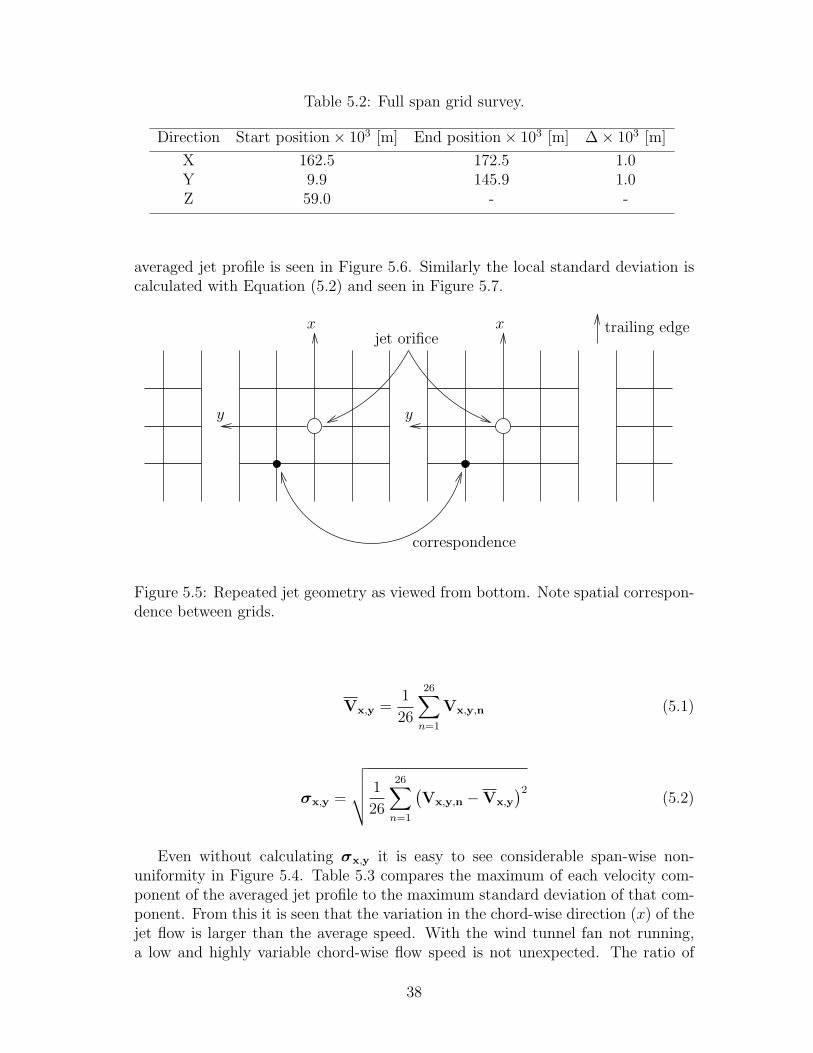
Table 5.2: Full span grid survey.

Direction Start position× 103 [m] End position× 103 [m] ∆× 103 [m]

X 162.5 172.5 1.0Y 9.9 145.9 1.0Z 59.0 - -

averaged jet profile is seen in Figure 5.6. Similarly the local standard deviation iscalculated with Equation (5.2) and seen in Figure 5.7.

xx

yy

jet orifice

correspondence

trailing edge

Figure 5.5: Repeated jet geometry as viewed from bottom. Note spatial correspon-dence between grids.

Vx,y =1

26

26∑n=1

Vx,y,n (5.1)

σx,y =

√√√√ 1

26

26∑n=1

(Vx,y,n −Vx,y

)2(5.2)

Even without calculating σx,y it is easy to see considerable span-wise non-uniformity in Figure 5.4. Table 5.3 compares the maximum of each velocity com-ponent of the averaged jet profile to the maximum standard deviation of that com-ponent. From this it is seen that the variation in the chord-wise direction (x) of thejet flow is larger than the average speed. With the wind tunnel fan not running,a low and highly variable chord-wise flow speed is not unexpected. The ratio of

38

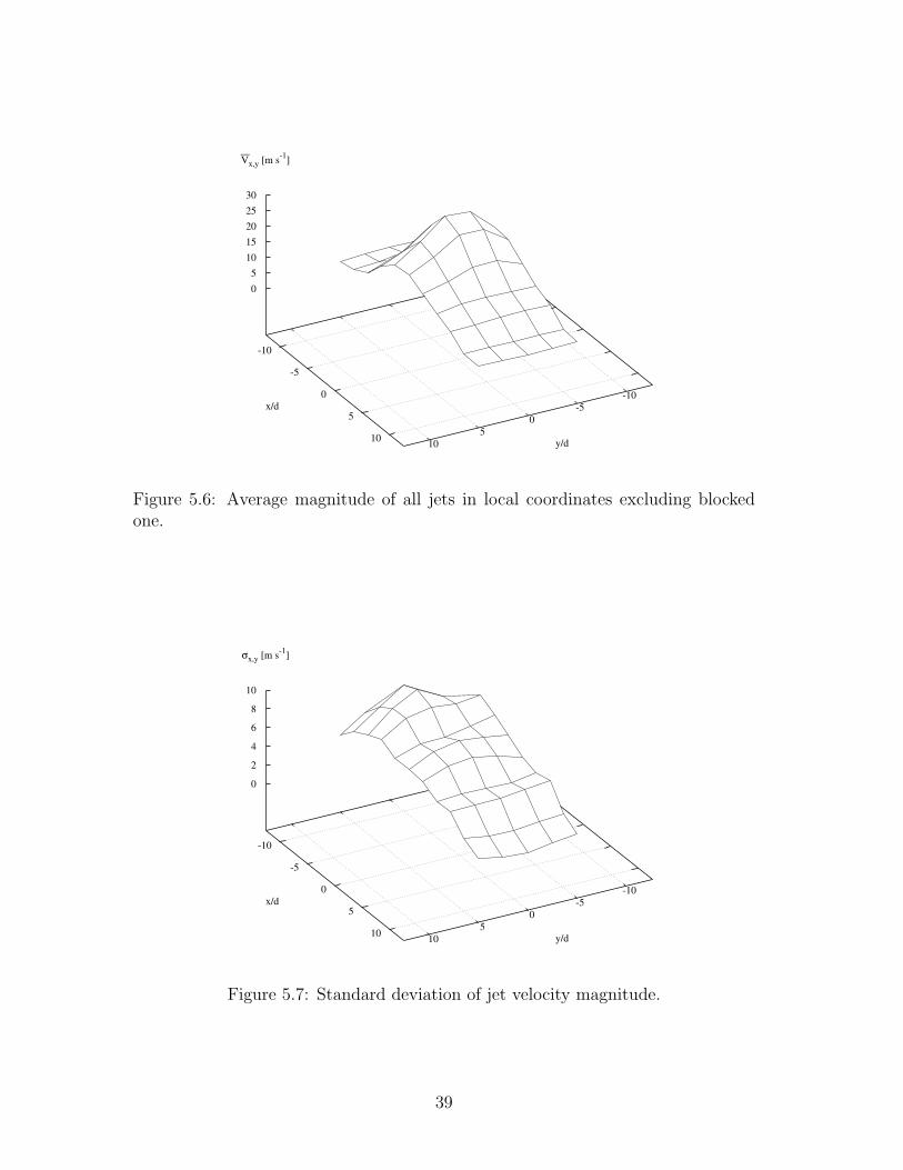
-10

-5

0

5

10

x/d-10

-5

0

5

10 y/d

0

5

10

15

20

25

30

Vx,y [m s-1

]

Figure 5.6: Average magnitude of all jets in local coordinates excluding blockedone.

-10

-5

0

5

10

x/d-10

-5

0

5

10 y/d

0

2

4

6

8

10

σx,y [m s-1

]

Figure 5.7: Standard deviation of jet velocity magnitude.

39

σx over Vx should be smaller with U∞ > 0. In the jet axial direction there is lessvariation in the flow speed, however it is still about one third of the mean value.One can easily see from these data that the series of jets do not closely simulate ablowing slot, though this does not necessarily imply ineffectiveness. The variationin the jets introduces three dimensionality into the flow and increases uncertaintyin correlations with Cµ. This three-dimensionality could cause increased mixing,more rapid jet decay, or other unknown effects.

Table 5.3: Comparison between maximum velocity and maximum standard devia-tion.

Direction Maximum Vx,y [m s−1] Maximum σx,y [m s−1]

x 4.82 5.75

z −27.4 9.48

Magnitude 27.6 9.18

5.3 Jet Momentum Integration

Using Simpson’s rule for double integrals (Equation 5.3) the momentum of the jetwas calculated. The derivation [27] of the rule shows that the weighting factor Wfollows a simple pattern as shown below. At low supply pressures, below thatrequired to achieve the critical pressure ratio (

pf

patm= 0.5283) [28], the flow from a

convergent nozzle should expand fully to atmospheric pressure at the outlet. Thisfact is easily seen by examining compressible flow tables. At higher supply pressuresthere will be some expansion beyond the jet outlet due to the sonic condition atthe throat.

M =∫ ∫

ρV Vdxdy = 19∆x∆y

∑x,y (W · ρV V) + O(∆x4) + O(∆y4) (5.3)

W =

1 4 2 4 . . . 2 4 14 16 8 16 8 16 42 8 4 8 4 8 24 16 8 16 8 16 4...

. . .

2 8 4 8 4 8 24 16 8 16 8 16 41 4 2 4 2 4 1

The results of momentum integration at distances: 24d (10× 10−3 m) and 38d

(15×10−3 m) (Figures 5.2(a) and (b)) are listed in Table 5.4. Immediately obvious

40

on examining the momentum results is that momentum is apparently not conservedwith increasing distance from the jet outlet. Momentum must be conserved how-ever, and free jets are no exception [29]. This suggests therefore, that there is someerror in the measurements or the calculations. The uncertainty on M was computedto be 10% at 24d and 8% at 38d (Section A.2). Thus the discrepancy between themomentum flux at the two cross sections is outside of the experimental uncertaintyand statistically significant. Although a decrease in measured momentum withdistance could be explained by some unaccounted loss or simply the diffusion ofmomentum outside the measured area, an increase should not occur since the jetitself is the only source.

Table 5.4: Momentum integrated over the cross-section. Note this is the momentumof one full jet plus two half jets.

Distance [ ] Mx × 103 [kg m s−2] Mz × 103 [kg m s−2] M × 103 [kg m s−2]

24d −2 25 25

38d −4 35 35

Since the momentum of the jet is proportional to the square of the velocity,it is particularly important to measure the peak velocity correctly. One potentialproblem is with the relative sizes of the LDA measurement volume and the jet. Asalready seen, the coincident measurement volume could be described as a spheroidof major dimension 396× 10−6 m and minor dimension 48.2× 10−6 m. Examiningthe flow fields presented in Figures 5.2(a) and (b) it is seen that the width of the jetsare roughly 10d (4×10−3 m). Hence in the stream-wise direction the probe width isapproximately 1% of the jet width, but in the span-wise direction the probe is 10%of the jet width. The length of the probe (396× 10−6 m) is comparable to the gridspacing ∆y of the jet measurement (Figure 5.2(a) and (b)), which is 500× 10−6 m.The result of a long probe in the span-wise direction is spatial averaging in thisdirection and possibly bias due to nonuniform particle seeding. If the particleseeding were non-uniform, and the cores of the jets had a lower concentration, thenone would expect that the measured velocities would be biased low. With uniformseeding and a large probe there is an equal chance of measuring a ‘fast’ or ‘slow’particle and averaging them. With nonuniform seeding there is a greater chance ofmeasuring the ‘slow’ particle, so the average is consequently lower. An examinationof the data rate shows a decrease in the rate at the location of each jet core in thenear field (24d) but not the far field (38d). Unfortunately no data were collectedon the time variation of the tunnel seeding. Thus it is possible, though unlikely,that the temporal variations coincided with the measurement of those particulargrid locations. Refer to Figures A.1(a) and (b) for the data rate surfaces.

41

5.4 Jet Momentum Comparison

The final LDA test conducted was intended to relate the momentum of the jet sheetto the measured flow rate ((qV )des). The jet momentum can be calculated usingthe mass flow rate (m), pressure (pf ), and an assumption of isentropic flow. Sincethe aforementioned method relies on an assumption, an independent LDA basedmethod was used for comparison. Velocity measurements were taken over threegrids surrounding the first, middle, and last jets over the full range of jet flow rates.The distance from the aerofoil surface was 43d. Due to time constraints, the sizeof the grids were limited, hence only the velocity around the core of the jets weremeasured. With the additional distance and the limited grid size, the whole jetprofiles were not captured. It was therefore not possible to numerically integratethe velocity field to obtain the jet momentum.

If the shape of the velocity profile were known, it might be possible to calculatethe total momentum of the jet, given that the maximum velocity was measured.An attempt was made to fit a curve to the full jet velocity fields presented inFigures 5.2(a) and (b). A reasonable hypothesis is that the velocity field of a singlejet in isolation is approximately Gaussian [29] in form far downstream in the fullydeveloped region. According to Pope [30] the profile of a round jet develops by about25d and a jet sheet by 40d. It is further reasonable to assume that superpositioncan be applied to determine the response of the entire row of jets and that theresponse resembles both the round jet and the jet sheet. The equation for the twodimensional Gaussian jet profile is:

Vj(x, y) = Vj,max · eln(0.5)·

»( x

wx)2+

“y

wy

”2–

(5.4)

where Vj,max is the maximum velocity of the jet and (wx, wy) are the half-widths ofthe jet. Refer to Section A.5 in the appendix for the development of this equation.

The half-widths of the jets in both profile surveys (Figures 5.2(a) and (b)) weremeasured and tabulated in Tables A.2 and A.3. The half-width wy differs from wx

due to interaction with the adjacent jets in the y direction. The average wx andwy are listed in Table 5.5 below. The average peak velocities are 53.8 m s−1 and

Table 5.5: Average half-widths of the jets at two distances.

Distance wx wy

[mm] [ ] [mm] [ ] [mm] [ ]

10 24d 1.2 3.0d 1.3 3.3d15 38d 1.7 4.3d 2.0 5.0d

43.7 m s−1 for the near and far locations respectively. If the square of Equation 5.4at three different grid locations is summed, then the square root of the sum gives

42

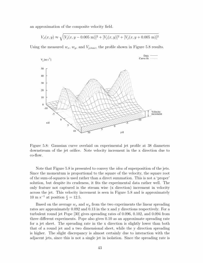
an approximation of the composite velocity field.

VJ(x, y) ≈√

[Vj(x, y − 0.005 m)]2 + [Vj(x, y)]2 + [Vj(x, y + 0.005 m)]2

Using the measured wx, wy, and Vj,max, the profile shown in Figure 5.8 results.

Velocityincrement

DataCurve fit

-10

-5

0

5

10

x/d-10

-5

0

5

10 y/d

0

10

20

30

40

50

Vj [m s-1

]

Figure 5.8: Gaussian curve overlaid on experimental jet profile at 38 diametersdownstream of the jet orifice. Note velocity increment in the x direction due toco-flow.

Note that Figure 5.8 is presented to convey the idea of superposition of the jets.Since the momentum is proportional to the square of the velocity, the square rootof the sum-of-squares is used rather than a direct summation. This is not a ‘proper’solution, but despite its crudeness, it fits the experimental data rather well. Theonly feature not captured is the stream wise (x direction) increment in velocityacross the jet. This velocity increment is seen in Figure 5.8 and is approximately10 m s−1 at position x

d= 12.5.

Based on the average wx and wy from the two experiments the linear spreadingrates are approximately 0.092 and 0.13 in the x and y directions respectively. For aturbulent round jet Pope [30] gives spreading rates of 0.096, 0.102, and 0.094 fromthree different experiments. Pope also gives 0.10 as an approximate spreading ratefor a jet sheet. The spreading rate in the x direction is slightly lower than boththat of a round jet and a two dimensional sheet, while the y direction spreadingis higher. The slight discrepancy is almost certainly due to interaction with theadjacent jets, since this is not a single jet in isolation. Since the spreading rate is

43

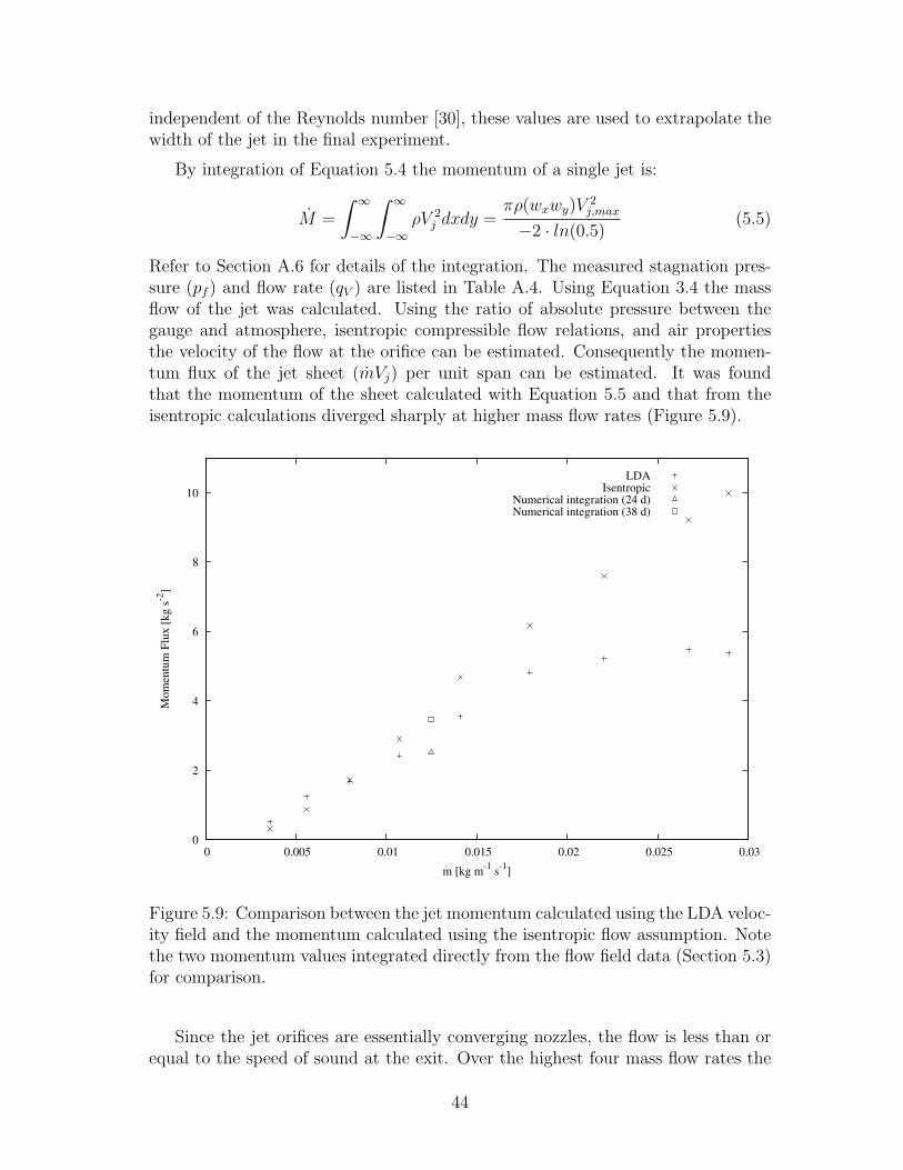
independent of the Reynolds number [30], these values are used to extrapolate thewidth of the jet in the final experiment.

By integration of Equation 5.4 the momentum of a single jet is:

M =

∫ ∞

−∞

∫ ∞

−∞ρV 2

j dxdy =πρ(wxwy)V

2j,max

−2 · ln(0.5)(5.5)

Refer to Section A.6 for details of the integration. The measured stagnation pres-sure (pf ) and flow rate (qV ) are listed in Table A.4. Using Equation 3.4 the massflow of the jet was calculated. Using the ratio of absolute pressure between thegauge and atmosphere, isentropic compressible flow relations, and air propertiesthe velocity of the flow at the orifice can be estimated. Consequently the momen-tum flux of the jet sheet (mVj) per unit span can be estimated. It was foundthat the momentum of the sheet calculated with Equation 5.5 and that from theisentropic calculations diverged sharply at higher mass flow rates (Figure 5.9).

0

2

4

6

8

10

0 0.005 0.01 0.015 0.02 0.025 0.03

Mo

men

tum

Flu

x [

kg

s-2

]

·m [kg m

-1 s

-1]

LDAIsentropic

Numerical integration (24 d)Numerical integration (38 d)

Figure 5.9: Comparison between the jet momentum calculated using the LDA veloc-ity field and the momentum calculated using the isentropic flow assumption. Notethe two momentum values integrated directly from the flow field data (Section 5.3)for comparison.

Since the jet orifices are essentially converging nozzles, the flow is less than orequal to the speed of sound at the exit. Over the highest four mass flow rates the

44

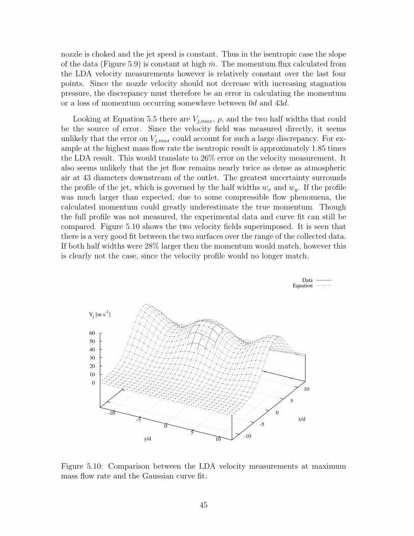
nozzle is choked and the jet speed is constant. Thus in the isentropic case the slopeof the data (Figure 5.9) is constant at high m. The momentum flux calculated fromthe LDA velocity measurements however is relatively constant over the last fourpoints. Since the nozzle velocity should not decrease with increasing stagnationpressure, the discrepancy must therefore be an error in calculating the momentumor a loss of momentum occurring somewhere between 0d and 43d.

Looking at Equation 5.5 there are Vj,max, ρ, and the two half widths that couldbe the source of error. Since the velocity field was measured directly, it seemsunlikely that the error on Vj,max could account for such a large discrepancy. For ex-ample at the highest mass flow rate the isentropic result is approximately 1.85 timesthe LDA result. This would translate to 26% error on the velocity measurement. Italso seems unlikely that the jet flow remains nearly twice as dense as atmosphericair at 43 diameters downstream of the outlet. The greatest uncertainty surroundsthe profile of the jet, which is governed by the half widths wx and wy. If the profilewas much larger than expected, due to some compressible flow phenomena, thecalculated momentum could greatly underestimate the true momentum. Thoughthe full profile was not measured, the experimental data and curve fit can still becompared. Figure 5.10 shows the two velocity fields superimposed. It is seen thatthere is a very good fit between the two surfaces over the range of the collected data.If both half widths were 28% larger then the momentum would match, however thisis clearly not the case, since the velocity profile would no longer match.

DataEquation

-10

-5

0

5

10

x/d-10

-5

0

5

10y/d

0

10

20

30

40

50

60

Vj [m s-1

]

Figure 5.10: Comparison between the LDA velocity measurements at maximummass flow rate and the Gaussian curve fit.

45

From the preceding it is concluded that there is a loss in momentum flux down-stream of the jet outlets, which limits the momentum observed in the far field. Itcan further be concluded that this loss is related to compressible flow as it onlyoccurs above the critical pressure ratio ( p∗

pf= 0.5283).

46

Chapter 6

Particle Image VelocimetryExperiment

The effect of the jet on the flow over the aerofoil was recorded with the particleimage velocimetry (PIV) method. A thorough description of the PIV method isgiven by Raffel et al. [24]. Digital image pairs of smoke particles in the wind tunnelare captured in rapid succession. During the time interval between frames (∆t), thesmoke particles shift position due to the flow velocity. Using a cross-correlation theparticle shift (∆X) between frames is determined for sub regions of the image. Anestimate of the instantaneous velocity in each sub region is calculated by ∆X/∆t.

6.1 Aerofoil Setup

The model aerofoil was clamped horizontally by the 6.35× 10−3 m air supply tubeat the centre line of the tunnel. Note that the aerofoil was mounted inverted inthe tunnel (Figure 6.1) so the positive lift direction is downward. The model waspivoted about the air supply tube to set the angle of attack.

flow direction

+α

‘suction surface’

‘pressure surface’

drag

lift

−θ

jet

Z

X

Figure 6.1: Aerofoil angle and force sign conventions.

47

6.2 Light Sheet Setup

A cross section of the smoke particles in the tunnel flow were illuminated by alaser light sheet. The pulsed light sheet serves both as the camera’s ‘flash’ and its‘shutter’. A Gemini PIV Nd:YAG laser, made by New Wave Research Incorporated,was used as the light source. The laser beam was divided with a beam splitter,spread into two sheets with cylindrical lenses, and reflected into the tunnel testsection. Figure 6.2 shows the two light sheets illuminating the flow field fromabove and below the model. Illumination from both sides was required to avoid ashadow directly above or below the aerofoil.

shadow lines

lower mirror

upper mirror

sheetedge of light

glass tunnel walls

Figure 6.2: Front view of double light sheet used in PIV experiment. Note the twosheets are coplanar.

48

laser

fan

mirror

lowermirror

sectiontest

upper

section

light sheet

sheet optic

beamsplittersheet optic

Figure 6.3: Side view of optical layout used in PIV experiment. Note light sheetsare perpendicular to the page.

6.3 Camera and Data Acquisition System Setup

The camera used to capture the flow was a Kodak MEGAPLUS ES 1.0 which hasa resolution of 1008 by 1018 pixels. The synchronization of the camera and laser,as well as the data acquisition was done using a FlowMap 1100 PIV processor andthe FlowManager 3.12.08 software made by Dantec Dynamics A/S.

The camera was set up on a heavy steel table in front of the tunnel test section(Figure 6.4) and was positioned such that the entire height of the test section wasimaged. The camera was then carefully focused on the mid-plane of the tunnel.

The scale factor for the images was determined by recording an image of a rulerset perpendicular to the camera at the focal plane. The camera, viewing area,and scale factor was checked before each set of tests to assure the setup remainedunaltered. Based on the camera resolution, a standard 32 by 32 pixel interrogationarea, and a 50% overlap of interrogation areas, a 62 by 62 vector field can becomputed. In the current experiment that translates to each vector representingan area of approximately 2.7× 10−3 m by 2.7× 10−3 m.

6.4 Experimental Cases

In the flow control experiment three parameters were varied: Cµ, α, and Re.

Eleven jet flow cases were chosen based on the gradations of the direct-readflow meter. The flow rates listed in Table A.4 have been converted to SI units and

49

compressed air in

back wall

front window

aero

foil

inflow

camera lens

ccd camera

camera focal plane

light sheet

Figure 6.4: Top view of PIV setup.

50

corrected for temperature and pressure as described in Chapter 3.

The wind tunnel fan was controlled by a variable frequency drive. The chosendrive frequencies for the experiment were the maximum possible (60 Hz) and 20 Hz.Thus half the data were collected at maximum Reynolds number and the other halfat approximately 30% of maximum. This was done in an attempt to distinguishReynolds number effects from α effects and jet momentum effects. The high andlow speed cases resulted in an overlap in Cµ over a useful range.

The nominal angles of attack chosen were 0◦, +5◦, +10◦, +15◦. The 15◦ casewas included at the suggestion that the 10◦ case might not fully capture the stallbehaviour of the system. The angle of attack is altered as a result of tunnel interfer-ence effects and the three dimensional nature of the flow. In the following sectionsit must be remembered that when angle of attack is referred to, it is the nominalangle of the aerofoil in tunnel coordinates, rather than the measured value.

It would have been desirable to specify values of Cµ and Re directly, insteadof varying a needle valve and a frequency controller, however this would have re-quired on-line measurements, calculations, and feedback. The tunnel speed andand air supply would have to be coordinated. Doing this manually would slowthe already lengthy process and introduce reading errors, since it would inevitablyrequire fractional flow meter settings.

6.5 Data Collection

The maximum frame rate in this system is limited by the aforementioned laser andis 7.5 Hz. It was suggested that some low frequency variation in the flow mightbe detectable. For this the highest sampling rate possible would be required andlosing synchronization (dropping frames) would be unacceptable. Due to memorylimitations, data transfer rate, and bulk storage usage only 37 sequential imageframes could be reliably acquired into one ensemble. The reason why one or twoextra frame pairs could occasionally be gathered is unknown. For each combinationof Cµ, α, and Re two ensembles of 37 image pairs were recorded. The entireexperiment was replicated three times to determine repeatability. During the laterPIV data analysis (Chapter 7) it was found that no useful time related informationcould be extracted from the data, so the above limitations were unnecessarily strict.In addition to the PIV image pairs, additional flow images were gathered withincreased smoke levels for qualitative flow observations.

A key parameter in any PIV setup is the inter-frame time, since the shift insmoke particles between images is proportional to this time interval. Obviously theparticle shift is also proportional to the speed of the flow, thus the time must beadjusted so that the particle displacement is not too large or too small. Based onapproximate tunnel speed and qualitative evaluation of a number of test ensembles,the inter-frame times were set to 25 µs and 100 µs for the low and high tunnel speedsrespectively.

51

Chapter 7

PIV Data Processing

The following chapter summarizes the methods used to process the raw imagesacquired and compute the lift coefficient and error at each momentum flux rate.First the cross-correlation that was performed on the digital images is outlined.The influence on the flow of the tunnel walls is then discussed. The method ofcalculating lift from the correlated images is detailed. The validity of pooling thedata to create a master set is stated. Finally the equations for calculating the errorin lift and momentum coefficients are given.

7.1 PIV Cross-correlation

The data were acquired with the Dantec FlowMap PIV system. During the dataacquisition process a selection of images were cross-correlated on the acquisitioncomputer to assure seeding and light levels were adequate. The main image pro-cessing and flow-map calculations however, were later done on a second computerusing the more recent Dantec DynamicStudio software.

Before correlation the raw images were intensity balanced. The reason for thiswas to minimize the effect of varying light intensity across the light sheet. Theintensity near the edges of the laser beam was found to vary slightly from pulse topulse. As seen in Figure 7.1 the aerofoil casts shadows both above and below. Solong as the intensity of an area is between the detection limit and saturation, goodcross correlations can be achieved. The problem is found at the edges of light anddark areas where erroneous vectors in the direction of the edge are often computed.Thus the edges of the shadows in the image would likely result in four rows ofvectors pointing up and down, while the remainder of the flow field would reflectthe dominant left to right flow. The image balancing algorithm reduces, but doesnot eliminate this problem.

One way to prevent the shadow lines is to illuminate from one side at a time(Figure 7.2). For the second and third replicates of the experiment the aerofoil wasilluminated from the top in the first 37 images and the bottom in the second 37

53

Figure 7.1: Example of raw flow-field image. Note light intensity is significantlyhigher than that used for data images. This was done for visualization purposes.

54

images. Using this method sacrifices the data in the shadow region, for improveddata in the remaining flow field. Thus the pairs of ensembles in the second andthird replicates must be used together to ‘see’ the entire field.

��������������������������������������������������������������������������������������������������������������������������������������������

��������������������������������������������������������������������������������������������������������������������������������������������

lower mirror

upper mirror

in shadowno good data

good data good data

good data

Figure 7.2: Schematic of single light sheet. Note shadow region that creates a ‘hole’in the vector field.

The balanced images were then cross-correlated using an adaptive scheme. Thisscheme uses 64 by 64 pixel interrogation areas to determine the general flow field.The general field is then refined using 32 by 32 pixel interrogation areas. Theadaptive scheme has a slight advantage in this case, since there are two distinctspeeds. There is the speed of the wind tunnel and there is the speed of the jet.Since the inter-frame time was optimized for the tunnel speed, the use of largerinterrogation areas results in more accurate correlations in the region of the jet. In

55

each case a 50% overlap in the interrogation areas was used.

Validation was done on the flow maps to ensure that only good data wererecorded. The peak validation threshold was set so that the dominant correlationpeak would be located rather than a noise peak. Peaks were accepted with pixeldisplacements between 2 and 5 pixels. The range of accepted stream-wise veloc-ities were −20 to 60 m s−1. The range of accepted cross-stream velocities were−25 to 25 m s−1. A large range in accepted velocities was used to encompass allcases, including those with strong recirculation and high jet velocities. The rangevalidation mainly functioned to remove spurious vectors, which were much largerthan the range values and obviously erroneous.

Following the validation, statistics were computed on the ensembles of 37 flowfields using DynamicStudio and the data were exported. Figure 7.3 is an exampleof the average vector field exported from DynamicStudio. No replaced vectors wereincluded in the exported data.

0

0.02

0.04

0.06

0.08

0.1

0.12

0.14

0 0.02 0.04 0.06 0.08 0.1 0.12 0.14 0.16

Z [

m]

X [m]

Figure 7.3: Example of 10◦ angle of attack at low speed with maximum jet flow rate.Note the ‘shadow line’ above the leading edge resulting from two sided illumination.

56

7.2 Correction of the Flow

When an aerofoil is placed in a wind tunnel, rather than an infinite body of air, theflow field is distorted by the presence of the impermeable walls. The classical wind-tunnel blockage corrections are described in depth in works such as “Low-SpeedWind Tunnel Testing” [20]. These corrections were not applied in this analysis,since the basic assumptions used to derive them are not correct in this case. Nat-urally the classical corrections do not account for the effect of the jet, which is adominant factor in the tunnel flow.

The derivation of the corrections begins by considering two-dimensional poten-tial flow around the aerofoil. In free air the streamlines away from the surface willbe curved because of the aerofoil. In tunnel flow the upper and lower walls presenta constraint on the flow in the vertical direction. Neglecting the tunnel wall bound-ary layer, the two walls effectively form straight streamlines at known locations. Tomodel this effect analytically, fictitious mirror images (Figure 7.4) of the aerofoilare placed periodically above and below the real aerofoil extending to infinity. Thiscauses straight streamlines to occur at the location of the walls in potential flow.The tunnel interference is the net effect of all of the images.

BA

D

C

Figure 7.4: Aerofoil mirror images. Note path of circulation integral.

57

In potential flow the aerofoil is modelled by superimposing sources, sinks, andpoint vortexes in the flow. This creates the effect of the solid shape, lift, andthe wake that is caused in real flow by viscous friction. The solid blockage effectof the aerofoil is modelled with one or more fluid sources and one or more fluidsinks arranged in the free stream. The lift of the aerofoil is modelled as eithera single point vortex or a distribution of point vortexes. Viscous effects and theaerofoil wake is represented by a source at the location of the aerofoil and a sinkfar downstream. The fluid source-sink pair act to displace the free stream outwardin the same manner as the lower momentum wake in viscous flow.

As detailed below in Section 7.3, the lift of the aerofoil is determined fromthe flow circulation, which in turn is calculated with a line integral enclosing theaerofoil and jet. The net effect of this method is that only sources of vorticitylocated within the line integral contribute to the circulation; the ‘image’ vortexsources being outside of the line. So long as the integration path encloses theaerofoil and jet, but excludes the wall boundary layers, the calculated lift will beunaffected by the presence of the walls. Interestingly this means that more thanone integration path will yield the same result within the precision of the method.

7.3 Lift and Drag Calculation

The circulation is computed on a path over the flow field (Figure 7.4). Due tomultiple factors the entire 62 by 62 vector field was not used. One reason was thatthe upper and lower walls are visible in the raw images (Figure 7.1) and obviouslythere are no valid vectors outside of the test section. The other factor is lightsheet variability at the edges. The left and right of the usable area are A and Brespectively. The bottom and top of the area are defined by C and D respectively.Note the flow field origin is in the lower left corner.

By the Kutta-Joukowski theorem the aerofoil lift coefficient is: Cl = 2ΓU∞c

[28].

In Cartesian coordinates the circulation about path P is simply Γ =∮

P(u · dX +

v · dZ) [24] for two dimensional flow in the (X,Z) plane. Note the importanceof encircling all vorticity generated by the aerofoil within the path P . Vorticitygeneration outside results in a bias in Γ, thus the importance of placing line segmentB sufficiently far downstream (ideally at X = ∞). For a rectangular path on auniform grid with spacing ∆ the equation is approximated by four sums:

Γ ≈ ∆ ·B∑

i=A

u(i, C) + ∆ ·D∑

j=C

v(B, j) + ∆ ·A∑

i=B

u(i, D) + ∆ ·C∑

j=D

v(A, j) (7.1)

The function was tested with a simulated uniform flow field at arbitrary angle,and with a simulated free vortex of strength Γ over varying paths. In each test the

58

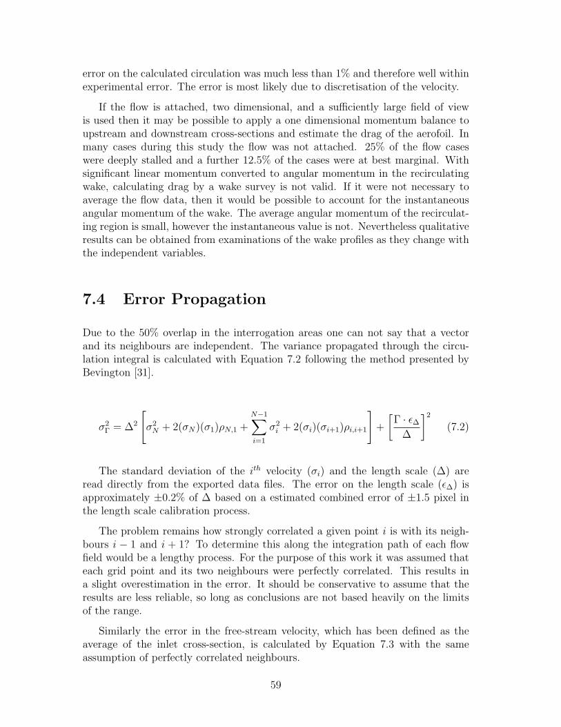
error on the calculated circulation was much less than 1% and therefore well withinexperimental error. The error is most likely due to discretisation of the velocity.

If the flow is attached, two dimensional, and a sufficiently large field of viewis used then it may be possible to apply a one dimensional momentum balance toupstream and downstream cross-sections and estimate the drag of the aerofoil. Inmany cases during this study the flow was not attached. 25% of the flow caseswere deeply stalled and a further 12.5% of the cases were at best marginal. Withsignificant linear momentum converted to angular momentum in the recirculatingwake, calculating drag by a wake survey is not valid. If it were not necessary toaverage the flow data, then it would be possible to account for the instantaneousangular momentum of the wake. The average angular momentum of the recirculat-ing region is small, however the instantaneous value is not. Nevertheless qualitativeresults can be obtained from examinations of the wake profiles as they change withthe independent variables.

7.4 Error Propagation

Due to the 50% overlap in the interrogation areas one can not say that a vectorand its neighbours are independent. The variance propagated through the circu-lation integral is calculated with Equation 7.2 following the method presented byBevington [31].

σ2Γ = ∆2

[σ2

N + 2(σN)(σ1)ρN,1 +N−1∑i=1

σ2i + 2(σi)(σi+1)ρi,i+1

]+

[Γ · ε∆

∆

]2

(7.2)

The standard deviation of the ith velocity (σi) and the length scale (∆) areread directly from the exported data files. The error on the length scale (ε∆) isapproximately ±0.2% of ∆ based on a estimated combined error of ±1.5 pixel inthe length scale calibration process.

The problem remains how strongly correlated a given point i is with its neigh-bours i − 1 and i + 1? To determine this along the integration path of each flowfield would be a lengthy process. For the purpose of this work it was assumed thateach grid point and its two neighbours were perfectly correlated. This results ina slight overestimation in the error. It should be conservative to assume that theresults are less reliable, so long as conclusions are not based heavily on the limitsof the range.

Similarly the error in the free-stream velocity, which has been defined as theaverage of the inlet cross-section, is calculated by Equation 7.3 with the sameassumption of perfectly correlated neighbours.

59

σ2U∞ =

1

N2

[σ2

N +N−1∑i=1

σ2i + 2 (σi) (σi+1) ρi,i+1

](7.3)

Based on the previously stated lift coefficient (Cl = 2ΓU∞c

) and Equations 7.2and 7.3 an expression for the variance of the lift coefficient was derived (7.4). Inthis expression the effect of the third term depends on whether the circulation ispositive or negative. If the circulation is positive the error in the lift is reduced byassuming a positive correlation between the free-stream velocity and the circulation.Alternatively if the circulation is negative, all else being equal, the third termincreases the calculated error. Again the error was overestimated by calculatingusing extreme values of correlation coefficient (ρΓ,U∞ = ±1) and recording whicheveris larger.

(σCl

Cl

)2

=(σΓ

Γ

)2

+

(σU∞

U∞

)2

− 2(σΓ

Γ

)(σU∞

U∞

)ρΓ,U∞ (7.4)

Combining the equations for the momentum coefficient (3.3, 3.4) results in Equa-tion 7.5. Using the same methods the expression for the error propagated throughto the momentum coefficient can be derived as in Equation 7.6.

Cµ =

(2

ρ∞ · c · s

)√k · (pf )des

R · (Tf )des

[√pf · (qV )des ·Ma

U2∞

](7.5)

(εCµ

Cµ

)2

=

(ε(qV )des

(qV )des

)2

+4

(σU∞

U∞

)2

+(εMa

Ma

)2

+1

4

(εpf

pf

)2

+2(εMa

Ma

)(εpf

pf

)ρMa,pf

(7.6)

Stated accuracy of the rotameter is ±5% full scale which is about ±1.2 ×10−4 m3 s−1. The accuracy of the pressure gauge is unknown. The manufacturer ofthe pressure gauge makes industrial gauges with ±1.6% full scale accuracy, whichis just under one half of the smallest division, but since no calibration informationis available the assumed accuracy is ±5% of full scale. The reading error on set-ting the flow rate results in a ±4% of value error on the pressure. Also there is a±1.7% slow fluctuation in the supply pressure. Thus the accuracy of the pressureis ±1.4× 104 Pa or better.

60

Chapter 8

PIV Data Pooling

For each combination of tunnel speed, angle of attack, and jet flow rate two en-sembles of 37 images were stored. Six to eight ensembles were initially recordedand checked as previously noted, however only the best two were kept. This wasrepeated three times, over a period of days, to assess repeatability. Thus for eachflow state there are six ensembles totalling 222 images, which in theory, could becombined to result in a master flow field or lift coefficient. Refer to Tables 8.1 and8.2 for a summary of the stored cases.

Table 8.1: Summary of PIV cases tested.

Parameter # Values

Chordal Reynolds number 2 0.038× 106 and 0.120× 106

Angles 4 0◦, 5◦, 10◦, and 15◦

Flow rates 11

Total cases 88

Table 8.2: Summary of data stored from PIV experiment.

Image pairs per ensemble 37Ensembles per case 2Replicates per case 3

Total image pairs per case 222

Due to the rate of data acquisition (7.5 Hz) it is reasonable to assume that eachimage in an ensemble is acquired under the same flow conditions, and is not subjectto long term variation or differences in the setup. For this reason the average flowfield was exported from DynamicStudio rather than all 37 individual flow fields.The two important questions are: how do the six ensemble-averaged flow fieldscompare and are they consistent?

61

The lift coefficient versus jet momentum curves for the first and second ensem-bles acquired can be compared. As mentioned previously the third ensemble cannotstand alone from the fourth and likewise the fifth from the sixth. This is a resultof the ‘hole’ in the flow map (Figure 7.2) either above or below the aerofoil due tothe shadow.

To compare the first and second ensembles the lift was computed for each setand averaged. The result is plotted versus Cµ in Figures 8.1(a) and (b). Errorbars are used to show the discrepancy between the two results. Clearly there aredifferences between the two ensembles at multiple points, however it is also clearthat the two data sets are comparable in both trend and magnitude. Thus thestatistics of the ensembles can be pooled within a replicate.

The statistics of each ensemble pair were pooled to create a master set for thegiven replicate. The lift and momentum flux were then recalculated resulting inFigures 8.2(a) through 8.6(b). In the 0◦ and 15◦ cases (Figures 8.2(a) and (b),8.6(a) and (b)), at both high and low Reynolds number, the trend is approximatelylinear. Clearly each of the three replicates, in these four cases, follows the samegeneral trend. Although the three replicates do not all fall on the same curve,Figure 8.2(b) in particular, the data can still be pooled.

Refer to Figures 8.3(a) and 8.4(a) for the 5◦ and 10◦ low Reynolds number casesrespectively. Though the two curves are different there is consistency between thedata of the three replicates. This is with exception to the region about Cµ = 0 inthe 5◦ case where replicate three diverges. Qualitatively it appears that the thirdreplicate is shifted in the negative Cµ direction.

In the 5◦ high Re case, and to a lesser extent the 0◦ high Re case, the threereplicates are similar in slope, but appear to be offset in the lift direction by aconstant. Alternatively the curves could be thought of as shifted in the momentumdirection, since changing the y- or x-intercept of a straight line has the same effect.One possible reason for this difference is the relatively crude apparatus for settingthe angle of attack. The angle of attack was measured, in tunnel coordinates,from the raw images. The true angle for each ensemble is presented in Tables B.1and B.2. The lift offset in the 5◦ high Re case follows the expected trend with α(Table B.2) and the 0◦ high Re case also does over a limited range. It is interestingto note that with decreasing measured α the previously mentioned low Re curvesat nominal 5◦ shift in the negative Cµ direction. Overall there is a trend in liftvalues with angle of attack between the replicates, however it cannot be concludedthat this is the only factor responsible for the variation between the replicates.Nevertheless it is still reasonable to conclude that the data of the three replicatesat 5◦, in high and low speed flow, are comparable.

The 10◦ high Reynolds number results are problematic. In the first replicatethe Cl begins at 0.98 and decreases smoothly with increasing Cµ as expected. Thesecond and third replicates do not follow this trend. The second and third replicatebegin at 0.64 and 0.87 respectively then drop sharply to approximately 0.1 at lowmomentum flux. The lift coefficient of these two curves behave erratically until they

62

-3.5

-3

-2.5

-2

-1.5

-1

-0.5

0

0.5

0 0.5 1 1.5 2 2.5 3 3.5

Cl

Cµ

0°5°

10°15°

(a) Lift-jet momentum at Re = 0.038× 106.

-0.4

-0.2

0

0.2

0.4

0.6

0.8

1

0 0.05 0.1 0.15 0.2 0.25 0.3

Cl

Cµ

0°5°

10°15°

(b) Lift-jet momentum at Re = 0.120× 106.

Figure 8.1: Mean lift computed from first and second ensemble. Note error barsindicating discrepancy between the individual ensembles and their mean.

63

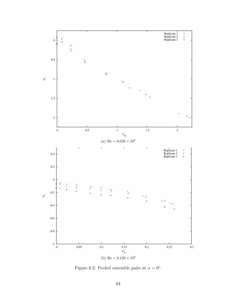
-2

-1.5

-1

-0.5

0

0 0.5 1 1.5 2

Cl

Cµ

Replicate 1Replicate 2Replicate 3

(a) Re = 0.038× 106

-1

-0.8

-0.6

-0.4

-0.2

0

0.2

0.4

0 0.05 0.1 0.15 0.2 0.25 0.3

Cl

Cµ

Replicate 1Replicate 2Replicate 3

(b) Re = 0.120× 106

Figure 8.2: Pooled ensemble pairs at α = 0◦.

64

-1.5

-1

-0.5

0

0.5

0 0.5 1 1.5 2

Cl

Cµ

Replicate 1Replicate 2Replicate 3

(a) Re = 0.038× 106

-0.4

-0.2

0

0.2

0.4

0.6

0.8

1

0 0.05 0.1 0.15 0.2 0.25 0.3

Cl

Cµ

Replicate 1Replicate 2Replicate 3

(b) Re = 0.120× 106

Figure 8.3: Pooled ensemble pairs at α = 5◦.

65

recover to the level of the smooth curve. The third curve recovers at Cµ = 0.11to Cl = 0.95. The second curve recovers later at Cµ = 0.16 to Cl = 0.86. It isinteresting to note from Table B.2 that the first replicate has the lowest measuredangle of attack followed by the third and the second replicates in that order. Thisresponse looks suspiciously like abrupt stall behaviour and suggests that the threereplicates in this case are not in fact comparable. Further evidence is provided byFigures 8.5(a) and (b), which show recirculation behind the aerofoil in the secondreplicate. One hypothesis for this behaviour is that the application of low jetmomentum has a destabilizing effect on the flow actually causing it to separate ifthe angle of attack is above a certain limit. A further hypothesis is that with asufficiently high momentum flux the flow will either remain attached or reattach.To confirm this behaviour the wake profile can be examined with increasing jet flowrate as shown in Figures 8.7, 8.8, and 8.9.

Figure 8.7 clearly shows a narrow wake that changes little with increasing jetflow rate. Figure 8.8 however shows a wake that varies irregularly in both widthand position with increasing jet flow before returning to a tightly confined wake atthe last four flow rates (Cµ ≥ 0.16). Figure 8.9 is perhaps the clearest example ofthe effect of momentum addition in this case. Initially the wake is narrow. Thewake immediately widens when a small jet flow is applied. As jet flow increasesthe wake narrows and at high momentum (Cµ = 0.11) the wake profile becomesS-shaped showing the decrease in velocity due to viscous effects and the increase invelocity due to jet momentum addition.

It can be said therefore, that the interpretation of the lift data is correct andthat under the right circumstances the jet can cause attached flow to separate justas it can cause separated flow to reattach. The conclusion drawn is that to avoidabrupt, and possibly dangerous, stall behaviour there is a minimum jet momentumthat should be applied when operating in marginal conditions.

Clearly it is worth being cautious about pooling the data, since in the 10◦ highReynolds number case this would result in misleading interpretations. With excep-tion to the 10◦ high speed case the statistics of the three replicates of the experimentwere pooled for each flow rate and angle of attack. For the high Reynolds number10◦ case the flow fields corresponding to the outliers in Figure 8.4(b) were discardedbefore calculating the new average flow field for each flow rate. The Cl versus Cµ

curves were subsequently recalculated for each case.

66

-1

-0.5

0

0.5

1

0 0.5 1 1.5 2

Cl

Cµ

Replicate 1Replicate 2Replicate 3

(a) Re = 0.038× 106

-0.2

0

0.2

0.4

0.6

0.8

1

1.2

0 0.05 0.1 0.15 0.2 0.25 0.3

Cl

Cµ

Replicate 1Replicate 2Replicate 3

(b) Re = 0.120× 106

Figure 8.4: Pooled ensemble pairs at α = 10◦.

67

0

0.02

0.04

0.06

0.08

0.1

0.12

0.14

0 0.02 0.04 0.06 0.08 0.1 0.12 0.14 0.16

Z [

m]

X [m]

(a) Replicate 1

0

0.02

0.04

0.06

0.08

0.1

0.12

0.14

0 0.02 0.04 0.06 0.08 0.1 0.12 0.14 0.16

Z [

m]

X [m]

(b) Replicate 2

Figure 8.5: Notice recirculating flow in replicate 2 is not seen in replicate 1. Nominalα = 10◦, Cµ = 0.02, Re = 0.120 × 106. Replicate 3 (not shown) similarly showsrecirculation.

68

-1

-0.5

0

0.5

1

0 0.5 1 1.5 2

Cl

Cµ

Replicate 1Replicate 2Replicate 3

(a) Re = 0.038× 106

-0.6

-0.4

-0.2

0

0.2

0.4

0.6

0 0.05 0.1 0.15 0.2 0.25 0.3

Cl

Cµ

Replicate 1Replicate 2Replicate 3

(b) Re = 0.120× 106

Figure 8.6: Pooled ensemble pairs at α = 15◦.

69

0

0.2

0.4

0.6

0.8

1

Z/h

u/U∞

Cµ

0.00

0.01

0.02

0.05

0.08

0.11

0.13

0.17

0.21

0.25

0.27

Figure 8.7: Wake profiles with increasing Cµ at 10◦ and Re = 0.120×106 (replicate1). Note also curves have been offset for clarity; vertical grid-lines indicate u

U∞= 1.

0

0.2

0.4

0.6

0.8

1

Z/h

u/U∞

Cµ

0.00

0.01

0.02

0.05

0.08

0.10

0.13

0.16

0.20

0.24

0.27

Figure 8.8: Wake profiles with increasing Cµ at 10◦ and Re = 0.120×106 (replicate2). Note also curves have been offset for clarity; vertical grid-lines indicate u

U∞= 1.

70

0

0.2

0.4

0.6

0.8

1

Z/h

u/U∞

Cµ

0.00

0.01

0.02

0.05

0.08

0.11

0.13

0.17

0.20

0.25

0.27

Figure 8.9: Wake profiles with increasing Cµ at 10◦ and Re = 0.120×106 (replicate3). Note also curves have been offset for clarity; vertical grid-lines indicate u

U∞= 1.

71

Chapter 9

Lift Control Results

The pooled results of the data processing are presented in the following sections.Low and high Reynolds number results are given with a general discussion of thetrends. The results are further compared with two prior works to check validity andunderstand the current trends. From this, an interpretation of the flow behaviouris drawn.

9.1 Low Speed Results

The low Reynolds number lift results from the current experiment are presentedbelow in Figure 9.1. As expected the lift coefficient decreases with increasing mo-mentum flux. One clear trend is the shift of the lift curves towards higher momen-tum flux with increasing angle of attack. This means that in general, the use ofjet flow to reduce the lift becomes less effective with increasing angle of attack. Indeep stall a large Cµ is required to affect significant control. Such levels may notbe practical or economical. With the exception of stall controlled machines thisoperational envelope is avoided anyway, so this may be inconsequential.

Notice in the figure that the highest four flow rates, at each angle of attack,follow the same trend as the preceding points. This provides incidental support forthe interpretation given in Chapter 5 that the loss in jet momentum occurs down-stream of the nozzle and is related to the nozzle pressure ratio. If the momentumcoefficient at the orifice were to approach a constant, then the lift coefficient shouldalso approach a constant. Cl clearly continues to increase in magnitude however,and there is no evidence to suggest that there should be a discontinuity at thisparticular location.

9.2 High Speed Results

The pooled high Reynolds number results are presented in Figure 9.2. As expectedincreased α results in increased Cl, and increased Cµ results in decreased Cl. At 15◦

73

-4

-3.5

-3

-2.5

-2

-1.5

-1

-0.5

0

0.5

0 0.5 1 1.5 2 2.5 3 3.5 4

Cl

Cµ

0°

5°

10°

15°

Figure 9.1: Pooled Cl versus Cµ curves at low Re.

the aerofoil is clearly stalled, thus it no longer follows either of the aforementionedtrends. Qualitatively the lift response with momentum flux is nearly linear with aslope on the order of one. A slightly concave downward trend is visible in Figure 9.2.

The definition of the momentum coefficient (Equation 2.1) shows how it is in-creasingly difficult to affect control as the free-stream velocity increases. In the‘high speed’ condition, which is still relatively low Re, the range of Cµ achievable isrelatively small. Since Cµ = f(U−2

∞ ) and Re = f(U∞), Cµ decreases faster than Reincreases with increasing U∞. This means that for a given Re, Cµ is increased bydecreasing U∞ and increasing the chord. In other words, if all else is equal, largeraerofoils should have larger ∆Cl.

It must be borne in mind that under the test conditions the 10◦ (nominal)experiment showed a very abrupt stall response, which is likely related to the lowmomentum boundary layer. The pooled results shown in Figure 9.2 represent thepre-stall response, however at slightly higher angle of attack the response wouldbe more similar to the 15◦ curve. It is therefore important to exercise caution ifoperation near stall is required; particularly if operating at low Reynolds number.

9.3 Comparison with Prior Work

Though the lift results calculated by the circulation integral are order-of-magnitudecorrect, it is worth comparing them to published data. Unfortunately much of the

74

-0.6

-0.4

-0.2

0

0.2

0.4

0.6

0.8

1

1.2

1.4

0 0.05 0.1 0.15 0.2 0.25 0.3

Cl

Cµ

0°

5°

10°

15°

Figure 9.2: Pooled Cl versus Cµ curves at high Re.

lift data published to date have been gathered at much higher Reynolds numbers.High Reynolds number lift data are not generally applicable to low Reynolds num-ber applications.

There are two obvious comparisons that can be made between prior work andthe current experiment. First the magnitude of Cl can be compared with classicwind-tunnel work if Cµ = 0. The Cl can be compared as α and Re are varied.Secondly Cl can be compared with previous jet flapped aerofoil results if α = 0.If the ‘natural’ circulation of the aerofoil (2παη) is zero (Section 2.2.1), then theresponse of the jet flap should be isolated. Thus the only difference between theelliptical aerofoil used by Dimmock [6] and the chosen NACA symmetric aerofoil isthe effect of the profile on the pressure component of lift.

9.3.1 Zero Momentum Flux Data

One data set used for comparison in this study was from Sheldahl and Klimasat Sandia National Laboratories [32]. The data were originally intended as aninput for wind turbine design. This data set was produced by combining in-houseexperimental data with synthesized data from a computer code. This was theonly data set found in the correct Reynolds number range for the NACA 0025aerofoil. It was tabulated by Reynolds number and angle of attack. Figure 9.3shows the comparison between the relatively sparse jet-off experimental data and

75

the comparison data. Note the experimental lift was plotted against true angle ofattack (Tables B.1 and B.2) rather than nominal. For example the nominally 0◦

data are actually plotted at −0.7◦ on the graph.

-0.4

-0.2

0

0.2

0.4

0.6

0.8

1

1.2

-4 -2 0 2 4 6 8 10 12 14 16 18

Cl

Angle of Attack [°]

Sandia Re=0.040×106

Sandia Re=0.080×106

Sandia Re=0.160×106

Re=0.038×106

Re=0.120×106

Figure 9.3: Lift curves for NACA 0025 aerofoil at three different Reynolds Num-bers [32] compared to the Cµ = 0 results from current experiment

It is seen that the data from the current experiment are somewhat consistentwith the comparison data set. At nominally 0◦ and 5◦ the current experiment isconsistent with the Sandia data. At the higher Re condition the current experimentshows the initial lift slope continuing to 10◦ before abruptly dropping to approxi-mately zero. The Sandia data, at similar Reynolds numbers, exhibit a much moregentle stall behaviour and significantly lower maximum lift. At the low Re conditionthe aerofoil in the current experiment appears to stall earlier somewhere between5◦ and 10◦. Thus in attached flow the two sets of results are consistent, howeverthe stall behaviour is very different. It is not known what factor or factors areresponsible for the discrepancies in lift and stall behaviour.

9.3.2 Zero Angle of Attack Data

For a symmetrical aerofoil section the nomenclature of ‘pressure side’ and ‘suctionside’ of the aerofoil can be interchanged. Thus the case of (α ≥ 0, θ ≤ 0) and(α ≤ 0, θ ≥ 0) are equivalent.

The data set used for zero angle of attack comparison was from Dimmock’sexperiments [6] detailed in Chapter 2. Figure 9.4 shows the current experimental

76

data, at high and low Reynolds number, compared with the predicted reaction lift(Equation 2.4). Compare the current experiment to Dimmock’s data at θ = 31.4◦

and 90.0◦. Note total lift curves (Equation 2.4) also plotted over Dimmock’s data.

-6

-5

-4

-3

-2

-1

0

0 1 2 3 4

Cl

Cµ

Re=0.038×106

Re=0.120×106

Natural + reaction lift (θ=-80°)

Re=0.147×106 to Re=0.425×10

6 (Dimmock)

Total lift (θ=-31.4°)

Re=0.425×106 (Dimmock)

Total lift (θ=-90.0°)

Figure 9.4: Comparison between current experimental data, published data [6], andthe predictions of Equation 2.4. Note the sign convention of published data wasinterchanged.

Immediately obvious is that the lift coefficient in the current experiment is muchsmaller in magnitude, for a given momentum flux, than the previous results. Sincethe current experiment uses a jet deflection angle of 80◦, the lift coefficients shouldfall somewhere between Dimmock’s results for θ = 31.4◦ and θ = 90.0◦. Thougha slight overestimate, Equation 2.4 fits the data reasonably well. The equationis within 5% at θ = 31.4◦ and 15% at θ = 90.0◦. The lift coefficient curve fromthe current experiment does not exhibit the expected

√Cµ behaviour. Rather

the reaction component of Equation 2.4 fits the data within uncertainty. Thus itappears that the significant ‘pressure lift’ component of the equation is missing.

Figure 9.5 gives a close up comparison between Dimmock’s results with andwithout trip wires, which were used to simulate an increase in Reynolds number. Inboth cases the measured Cl values converge onto the predicted curve with increasingCµ. Notice that the case with the trip wire is closer to the predicted curve. Whilethe high Reynolds number results in Figure 9.4 do exhibit a slight curvature, it isnot possible to say if the lift would converge onto the expected curve at a sufficientlyhigh Cµ.

77

-1.2

-1

-0.8

-0.6

-0.4

-0.2

0

0 0.05 0.1 0.15 0.2 0.25 0.3

Cl

Cµ

No trip wireTrip wireEquation

Figure 9.5: Effect of tripping the boundary layer: α = 0◦, θ = −31.4◦, Re = 0.425×106. All data from Dimmock [6].

9.4 Pressure Lift

From examining the low and high Reynolds results, and comparing them to previousresults it is clear that the current experimental results do not show the characteristic‘pressure lift’ effect. It is therefore worth investigating why this important compo-nent is not exhibited. As before, a qualitative examination of the wake profiles inFigures 9.6(a), 9.6(b), 9.7(a), and 9.7(b) reveals what occurs in the flow.

In Figures 9.6(a) and (b) it is seen that the wake initially narrows with increasingCµ. This is the well known aerofoil boundary layer control effect of momentuminjection. With increasing Cµ the trend reverses and the wake widens greatly. Alarge wake represents a large loss in momentum, which is not an expected resultof momentum injection. Notice that in the 0◦ case, where the magnitude of lift isgreater than that of the 5◦ case, the wake is also larger. The 10◦ and 15◦ wakeprofiles follow the same trends as the lower angles of attack. With a larger angle ofattack the initial wake is deeper and the smallest wake occurs at higher Cµ. Againthe final wake is smaller with increasing angle of attack and decreasing magnitude oflift. The loss in flow momentum with larger Cµ is a result of the jet forcing the flowto separate at the trailing edge behind the jet. This is analogous to the increasein drag and loss of lift due to locating a Gurney flap ahead of the trailing edge(Section 2.3.3). This observation is also supported by a qualitative examination

78

0

0.2

0.4

0.6

0.8

1

Z/h

u/U∞

Cµ

0.0

0.1

0.2

0.5

0.8

1.1

1.5

2.1

2.7

3.3

3.5

(a) α = 0◦

0

0.2

0.4

0.6

0.8

1

Z/h

u/U∞

Cµ

0.0

0.1

0.2

0.5

0.7

1.0

1.2

1.6

2.2

2.8

3.1

(b) α = 5◦

Figure 9.6: Low speed flow wake profiles for 0◦ and 5◦ listed by Cµ. Note againcurves are offset for clarity; grid-lines indicate u

U∞= 1.

79

0

0.2

0.4

0.6

0.8

1

Z/h

u/U∞

Cµ

0.0

0.1

0.2

0.5

0.8

1.0

1.2

1.5

1.8

2.2

2.4

(a) α = 10◦

0

0.2

0.4

0.6

0.8

1

Z/h

u/U∞

Cµ

0.0

0.1

0.2

0.5

0.8

1.0

1.2

1.6

1.8

2.1

2.3

(b) α = 15◦

Figure 9.7: Low speed flow wake profiles for 10◦ and 15◦ listed by Cµ. Note againcurves are offset for clarity; grid-lines indicate u

U∞= 1.

80

of flow visualization images. Figure 9.8 is an example of one such image. Unlikethe aforementioned low speed wake profiles, the high speed wake profiles revealnothing particularly interesting about the flow over the limited range of Cµ. Referto Section B.2 in the appendix for the high Re wake profiles.

‘pressure surface’ jet

separation

trailing edge separation

transition/reattachment

Figure 9.8: Flow visualization image of aerofoil at 10◦, Cµ = 0.5, and Re = 0.038×106. Note the separation and reattachment over the aerofoil as well as the trailingedge separation.

9.5 Pressure Lift Replacement

Interesting parallels can be drawn between Dimmock’s results (Figure 9.5) if the‘missing’ pressure lift is replaced. In effect this is adding the lift as follows:

Cl = Cl,measured +(3.9√

Cµ

)sin(θ + α) (9.1)

Though this seems artificial, it allows flow separation effects to be observed apartfrom the trailing edge separation. The result of adding in this term is shown inFigure 9.9(a) through 9.10(b).

Figures 9.9(a) and (b) show how, with this method, the data collapse down ontothe predicted curve. The more interesting result is the deviation from the predictedcurve of the lift coefficient in Figures 9.10(a) and (b). Notice that in the 10◦ highspeed case the measured lift slightly exceeds the expected lift in magnitude. At thesame angle of attack and lower speed the lift deviates more from what is expected.Similarly at α = 15◦ (Figure 9.10(b)) both high and low Reynolds number curvesexceed in magnitude the expected lift. Notice that the low Re data at both 10◦ and15◦ converge onto the expected curve with increasing Cµ. Note that in the publisheddata (Figure 9.5) the data follows the same trend, however on the opposite side ofthe predicted curve.

81

The explanation for this behaviour is flow separation on the ‘suction surface’as shown in Figures 6.1 and 9.8. This is the same surface that the jet is locatedon. Due to flow separation the ‘natural’ component (2παη) of lift is diminished, sothe jet is more effective in a relative sense, and the magnitude of lift is thereforegreater. As Cµ is increased it has a boundary layer control effect causing the flowto reattach and the ‘natural’ lift to increase working against the ‘pressure’ and‘reaction’ components. Note that at 10◦ and low Re the data fall on the predictedcurve at fifth and higher jet momentum rates, and at 15◦ on the seventh. Referringback to Figures 9.7(a) and (b) it is seen that the wake narrows at approximatelythe fifth wake and seventh wake profiles respectively. Qualitatively these are alsothe flow rates at which the jet velocity becomes visible in the profiles.

In essence the aforementioned effect is the result of placing the jet on the ‘suctionsurface’ of the aerofoil. More accurately this is the effect of setting (θ ≤ 0, α ≥ 0)or (θ ≥ 0, α ≤ 0). From a control perspective it is problematic to have a controlaction respond in an opposite manner under a limited set of conditions. Thus fromthe control perspective at lower Reynolds numbers it is advantageous to locate thecontrol jet on the ‘pressure surface’ of the aerofoil.

82

-12

-10

-8

-6

-4

-2

0

2

0 0.5 1 1.5 2 2.5 3 3.5 4

Cl

Cµ

Low ReHigh Re

Equation

(a) 0◦

-12

-10

-8

-6

-4

-2

0

2

0 0.5 1 1.5 2 2.5 3 3.5 4

Cl

Cµ

Low ReHigh Re

Equation

(b) 5◦

Figure 9.9: Low and high Reynolds number data at 0◦ and 5◦ with ‘replaced’pressure lift.

83

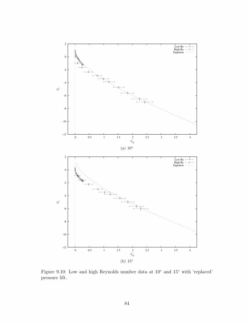
-12

-10

-8

-6

-4

-2

0

2

0 0.5 1 1.5 2 2.5 3 3.5 4

Cl

Cµ

Low ReHigh Re

Equation

(a) 10◦

-12

-10

-8

-6

-4

-2

0

2

0 0.5 1 1.5 2 2.5 3 3.5 4

Cl

Cµ

Low ReHigh Re

Equation

(b) 15◦

Figure 9.10: Low and high Reynolds number data at 10◦ and 15◦ with ‘replaced’pressure lift.

84

Chapter 10

Conclusions andRecommendations

10.1 Conclusions

A jet control sheet and its accompanying air supply system can be fabricated in aconventional aerofoil with simple practical manufacturing methods. In particular arow of discrete drilled outlets can be used as an alternative to a continuous slot.

Although discrete air jets are not uniform in either the near or far field, theindividual jets do spread and merge to form a jet sheet. Differences between theshape and angle of the drilled holes leads to variation in the jet profile from whatis expected.

The simple jet orifices were subject to large losses when the supply pressurewas raised above the critical pressure ratio, hence the pressure should not be raisedabove this level unless the nozzle shape is refined.

In general there is a limitation on the upper range of practical free-stream ve-locities for jet control, since Cµ ∝ U−2

∞ . It was found that there are also significantlimitations to the effectiveness of jet control in very low Reynolds number regimes(Re ≈ 105), hence this method is most appropriate for moderate Reynolds numberwind turbines. In low Reynolds number flows the jet has a significant boundarylayer control effect through jet entrainment. Under conditions of natural flow sep-aration, such as high angle of attack, momentum from the jet is absorbed by thethick boundary layer and the wake. It was found that near stall low levels ofCµ caused flow separation from the aerofoil surface, while at high levels it causedreattachment.

Practical aerofoils typically have sharp trailing edges. If a sharp trailing edgeis used then the control jet must be located forward of this position. Locating thecontrol jet at 9% forward of the trailing edge has a detrimental effect on both thelift and drag of the aerofoil. With the given configuration the jet acts to separatethe flow at the trailing edge, which increases drag and prevents ‘pressure lift’ from

85

being generated over the aerofoil. Thus the only modification of lifting force isthrough the jet reaction thrust itself.

In low Reynolds number flow the effect of negative jet deflection angle, combinedwith positive angle of attack, is that the boundary layer control acts counter to theintended ‘flap action’. The opposing control effect, along with the aforementionedforced flow separation, lead to the conclusion that this is not a good control methodfor low Reynolds number flow regimes.

10.2 Recommendations

It is recommended that proportionally smaller, but more frequent, jet outlets shouldbe used. This would be particularly easy if larger aerofoil models were constructed.More frequent outlets should lead to a more uniform flow in the near field, whichis more similar to a sheet.

If possible further testing should be conducted at higher Reynolds number todetermine if the large separated wake occurs under this condition and if there isevidence of ‘pressure lift’. If higher Reynolds number testing cannot be done thenthe use of trip wires should be attempted to simulate higher Reynolds number flow.

Experimentation with a smaller jet deflection angle is recommended to deter-mine if trailing edge separation can be avoided at low Reynolds number. Testswith a slightly truncated and rounded trailing edge could be done to determineif separation can be minimized in this way. It is possible that this, or a similarsystem, could be useful on inboard truncated wind turbine aerofoils [33].

It is worth investigating if the use of periodic jet flow can prevent flow separation,either over the aerofoil or at the trailing edge, and improve performance. Both thefrequency and the duty cycle of the jet flow could be varied to study the response.

Finally it is recommended that, once effective control of steady flow has beenestablished, the step-change and sinusoidally-varying angle of attack cases be in-vestigated.

86

References

[1] T. Burton, D Sharpe, N. Jenkins, and E. Bossanyi. Wind Energy Handbook,chapter 8.3.9, pages 492–493. John Wiley and Sons, Toronto, 2001.

[2] T. J. Larsen, H. A. Madsen, and K. Thomsen. Active load reduction us-ing individual pitch, based on local blade flow measurements. Wind Energy,8(1):67–80, 2005.

[3] L. W. Carr. Progress in analysis and prediction of dynamic stall. Journal ofAircraft, 25(1):6–17, January 1988.

[4] S. Schreck and M. Robinson. Blade three-dimensional dynamic stall responseto wind turbine operating condition. Journal of Solar Energy Engineering,127:488–495, 2005.

[5] M. M. Hand, D. A. Simms, L. J. Fingersh, D. W. Jager, J. R. Cotrell,S. Schreck, and S. M. Larwood. Unsteady aerodynamics experiment phasevi: Wind tunnel test configurations and available data campaigns. Techni-cal Report TP-500-29955, National Renewable Energy Laboratory, December2001.

[6] N. A. Dimmock. An experimental introduction to the jet flap. Current Paper344, Aeronautical Research Council, London, 1957.

[7] G. K. Korbacher and K. Sridhar. A review of the jet flap. UTIA Review 14,University of Toronto, May 1960.

[8] B. Massey and J. Ward-Smith. Mechanics of Fluids, pages 108–109. Taylorand Francis, New York, eighth edition, 2006.

[9] T. Strand. The jet flap: review and extension. Convair division report, GeneralDynamics Corporation, 1956.

[10] D. A. Spence. The lift coefficient of a thin, jet-flapped wing. Proceedings ofthe Royal Society A, 238(1212):46–68, December 1956.

[11] B. S. Stratford. Mixing and the jet flap. The Aeronautical Quarterly, 7(2):85–105, May 1956.

87

[12] B. S. Stratford. A further discussion on mixing and the jet flap. The Aeronau-tical Quarterly, 7(3):169–183, August 1956.

[13] C. Tongchitpakdee, S. Benjanirat, and N. S. Sankar. Numerical studies of theeffects of active and passive circulation enhancement concepts on wind turbineperformance. Journal of Solar Energy Engineering, 128:432–444, 2006.

[14] L. W. Traub, A. C. Miller, and O. Rediniotis. Comparisons of a gurney andjet flap for hingeless control. Journal of Aircraft, 41(2):420–423, 2004.

[15] D. A. Spence. Some simple results for two-dimensional jet-flap aerofoils. TheAeronautical Quarterly, 9:395–406, 1958.

[16] D. T. Y. Nakafuji, C. P. van Dam, R. L. Smith, and S. D. Collins. Activeload control for airfoils using microtabs. Journal of Solar Energy Engineering,123:282–289, 2001.

[17] T. Buhl, M. Gaunaa, and C. Bak. Potential load reduction using airfoils withvariable trailing edge geometry. Journal of Solar Energy Engineering, 127:503–516, 2005.

[18] B. Sperandei. The application of particle image velocimetry in a small scalewind tunnel. Master’s thesis, University of Waterloo, November 2002.

[19] R. C. Pankhurst and D. W. Holder. Wind-Tunnel Technique. Sir Isaac Pitmanand Sons, Ltd., Toronto, 1952.

[20] Rae W. H. Jr. and Pope A. Low-Speed Wind Tunnel Testing. John Wiley andSons, New York, 1984.

[21] E. N. Jacobs, K. E. Ward, and R. M. Pinkerton. The characteristics of 78 re-lated aerofoil sections from tests in the variable-density wind tunnel. TechnicalReport 460, National Advisory Committee for Aeronautics, January 1933.

[22] Photograph by Stephen Orlando, January 2010.

[23] R. W. Miller. Flow Measurement Engineering Handbook, chapter 14, pages40–48. McGraw-Hill, third edition, 1996.

[24] M. Raffel, C. Willert, and J. Kompenhans. Particle Image Velocimetry.Springer-Verlag, New York, 1998.

[25] H. E. Albrecht, M. Borys, N. Damaschke, and C. Tropea. Laser Doppler andPhase Doppler Measurement Techniques. Springer-Verlag, New York, 2003.

[26] M. Young. Optics and Lasers. Springer-Verlag, New York, second edition,1984.

[27] M. G. Salvadori and M. L. Baron. Numerical Methods in Engineering. Prentice-Hall, New York, 1952.

88

[28] F. M. White. Fluid Mechanics. McGraw-Hill, New York, 2003.

[29] H. Schlichting. Boundary-Layer Theory. McGraw-Hill, Toronto, seventh edi-tion, 1987.

[30] S.B. Pope. Turbulent Flows. Cambridge University Press, New York, 2006.

[31] P. R. Bevington. Data Reduction and Error Analysis for the Physical Sciences.McGraw-Hill, New York, 1969.

[32] R. E. Sheldahl and P. C. Klimas. Aerodynamic characteristics of seven symmet-rical airfoil sections through 180-degree angle of attack for use in aerodynamicanalysis of vertical axis wind turbines. Energy Report SAND80-2114, SandiaNational Laboratories, Albuquerque, March 1981.

[33] S. P. Law and Gregorek G. M. Wind tunnel evaluation of a truncated naca64-621 airfoil for wind turbine applications. Technical Report CR-180803,National Aeronautics and Space Administration, July 1987.

89

APPENDICES

91

Appendix A

Ancillary Information on JetExperiment

A.1 Beam Properties

Table A.1: LDA beam properties.

Parameter Symbol Value

Beam expander ratio - 1.98Initial beam diameter - 2.16× 10−3 mBeam diameter before focusing 2 · wf 4.28× 10−3 mBeam separation before expansion - 38.1× 10−3 mBeam separation distance ds 75.4× 10−3 mLens focal length f 310× 10−3 mDistance of focal point along beam l(ds, f) 312× 10−3 m

LDA beam intersection half-angle φ2

0.121 rad

93

A.2 Jet Momentum Integration Uncertainty

σMx≈

√√√√∑x,y

[Wρ∆x∆yVxVz

9

]2[(

ερ

ρ

)2

+(ε∆x

∆x

)2

+

(ε∆y

∆y

)2

+

(σVx

Vx

)2

+

(σVz

Vz

)2]

(A.1)

σMz≈

√√√√∑x,y

[Wρ∆x∆yV 2

z

9

]2[(

ερ

ρ

)2

+(ε∆x

∆x

)2

+

(ε∆y

∆y

)2

+

(2σVz

Vz

)2]

(A.2)

σM =1

M

√(σMx

Mx

)2

+(σMz

Mz

)2

(A.3)

94

A.3 LDA Data Rate

-10

-5

0

5

10

x/d-10

-5

0

5

10 y/d

0

5000

10000

15000

20000

25000

30000

35000

Data Rate [s-1

]

(a) 24d from jet orifice

-10

-5

0

5

10

x/d-10

-5

0

5

10 y/d

0

5000

10000

15000

20000

25000

30000

35000

Data Rate [s-1

]

(b) 38d from jet orifice

Figure A.1: LDA data rate. Note arrow in Figure A.1(a) showing distinct dimpleat the centre of the grid not seen in Figure A.1(b).

95

A.4 Measured Jet Properties

Table A.2: Jet half widths at 10× 10−3 m cross section (all in mm).

DirectionJet 13 Jet 14 Jet 15 Average

w+ w− w+ w− w+ w− w

x 1.1 1.0 1.3 1.0 1.4 1.2 1.2y 1.2 - 1.4 1.3 - 1.5 1.3

Table A.3: Jet half widths at 15× 10−3 m cross section (all in mm).

DirectionJet 13 Jet 14 Jet 15 Average

w+ w− w+ w− w+ w− w

x 1.8 1.3 2.1 1.3 1.8 1.8 1.7y 2.0 - 1.7 2.2 - 2.2 2.0

Table A.4: Stagnation pressure and pressure ratios with flow rate. Note p∗ is thepressure at the orifice and patm is atmospheric pressure.

qV × 106 [m3 s−1] pf × 10−3 [Pa] (absolute) p∗

pf

p∗

patm

386 106 0.957 1.000552 116 0.870 1.000690 132 0.766 1.000802 153 0.662 1.000840 170 0.595 1.000878 184 0.550 1.000940 219 0.528 1.139998 253 0.528 1.3191041 294 0.528 1.5351077 308 0.528 1.607

96

A.5 Equation of Two Dimensional Jet Profile

Schlichting [29] suggests the following equation to describe a jet velocity (u) interms of the centre-line velocity (um) and the free stream velocity (U∞):

u2 − U2∞

u2m − U2

∞= e−ln(2)·( y

b )2

where the width b is defined as the jet width, in terms of momentum, so that ify = b then

u2 − U2∞

u2m − U2

∞=

1

2

In the LDA experiment the free stream velocity is zero, so the above equationis simplified somewhat. Alternatively the jet half radius (r1/2) can be defined interms of the location where the velocity is half that of the centre-line followingPope [30]. This requires the constant in the exponential to be changed to ln(0.5)so that at radial location r = r1/2 the jet velocity is 1

2Vj,max. Thus the velocity in

polar coordinates is:

Vj = Vj,max · eln(0.5)·

„r

r1/2

«2

For non rotationally symmetric distributions the(

rr1/2

)2

term can be replaced with

its multidimensional equivalent(

xwx

)2

+(

ywy

)2

. Thus the full equation becomes:

Vj = Vj,max · eln(0.5)·

»( x

wx)2+

“y

wy

”2–

If the major and minor axes are equal (wx = wy) then the equation becomesequivalent to the rotationally symmetric equation above.

A.6 Momentum Integral

The equation of the jet velocity is:

Vj = Vj,max · eln(0.5)·

»( x

wx)2+

“y+δwy

”2–

For a row of n jets the sum of squared velocities is:

V 2J = V 2

j,max · e2·ln(0.5)·

»( x

wx)2+

“y+δ1wy

”2–+ . . . + V 2

j,max · e2·ln(0.5)·

»( x

wx)2+

“y+δn

wy

”2–

97

Substituting into the momentum flux equation and integrating:

Mn =

∫ ∞

−∞

∫ ∞

−∞ρ(V 2

J

)dxdy

=

∫ ∞

−∞

∫ ∞

−∞ρ

(V 2

j,max · e2·ln(0.5)·

»( x

wx)2+

“y+δ1wy

”2–+ . . .

)dxdy

= ρV 2j,max

[∫ ∞

−∞

∫ ∞

−∞e2·ln(0.5)

“y+δ1wy

”2

e2·ln(0.5)( xwx

)2

dxdy + . . .

]= ρV 2

j,max

[∫ ∞

−∞

(e2·ln(0.5)

“y+δ1wy

”2∫ ∞

−∞e2·ln(0.5)( x

wx)2

dx

)dy + . . .

]

Since∫∞−∞ e−ax2

dx =√

πa

then set a = −2·ln(0.5)w2

x

Mn = ρV 2j,max

[wx

√−π

2 · ln(0.5)

∫ ∞

−∞e2·ln(0.5)

“y+δ1wy

”2

dy + ...

]= ρV 2

j,max

[wx

√−π

2 · ln(0.5)

(e2·ln(0.5)

“δ1wy

”2∫ ∞

−∞e

2·ln(0.5)

w2y

y2

e2

2δ1·ln(0.5)

w2y

ydy

)+ ...

]

Since∫∞−∞ e−ay2

e−2bydy =√

πae

b2

a then set a = −2·ln(0.5)w2

y, b = −2δ1·ln(0.5)

w2y

Mn = ρV 2j,max

[wx

√−π

2 · ln(0.5)e2·ln(0.5)

“δ1wy

”2

wy

√−π

2 · ln(0.5)e−2·ln(0.5)

“δ1wy

”2

+ . . .

]= ρV 2

j,max

[π(wxwy)

−2 · ln(0.5)+

π(wxwy)

−2 · ln(0.5)+ . . . +

π(wxwy)

−2 · ln(0.5)

]=

πρ(wxwy)V2j,max

−2 · ln(0.5)× n

98

Appendix B

Ancillary Information on LiftControl Experiment

B.1 Measured Angle of Attack in PIV Experi-

ment

Table B.1: Measured α at low Re for each ensemble and nominal α in degrees.

NominalEnsembles

Average1 2 3 4 5 6

0 -0.87 -1.05 -0.58 -0.22 -1.05 -0.87 -0.775 6.26 6.21 5.07 5.07 4.19 4.30 5.1810 9.18 9.32 10.19 10.27 10.32 10.39 9.9515 14.66 14.96 14.75 14.36 14.39 14.50 14.60

Table B.2: Measured α at high Re for each ensemble and nominal α in degrees.

NominalEnsembles

Average1 2 3 4 5 6

0 -0.93 -0.75 -0.40 -0.34 -1.17 -0.87 -0.745 6.87 6.35 5.34 5.26 4.52 4.22 5.4310 9.32 9.65 10.88 10.67 10.70 10.73 10.3315 14.38 14.90 14.41 14.85 14.75 14.96 14.71

99

B.2 Wake Profiles from PIV Experiment

0

0.2

0.4

0.6

0.8

1

Z/h

u/U∞

Cµ

0.00

0.01

0.02

0.04

0.08

0.10

0.12

0.16

0.20

0.24

0.26

(a) α = 0◦

0

0.2

0.4

0.6

0.8

1

Z/h

u/U∞

Cµ

0.00

0.01

0.02

0.05

0.08

0.10

0.12

0.16

0.20

0.24

0.26

(b) α = 5◦

Figure B.1: High speed flow wake profiles for 0◦ and 5◦ listed by Cµ. Note againcurves are offset for clarity; grid-lines indicate u

U∞= 1.

100

0

0.2

0.4

0.6

0.8

1

Z/h

u/U∞

Cµ

0.00

0.01

0.02

0.05

0.08

0.11

0.13

0.17

0.20

0.25

0.27

(a) α = 10◦

0

0.2

0.4

0.6

0.8

1

Z/h

u/U∞

Cµ

0.00

0.01

0.02

0.05

0.08

0.11

0.13

0.17

0.21

0.26

0.28

(b) α = 15◦

Figure B.2: High speed flow wake profiles for 10◦ and 15◦ listed by Cµ. Note againcurves are offset for clarity; grid-lines indicate u

U∞= 1.

101