AIR FORCE INSTITUTE OF TECHNOLOGY · explaining the concept of chaos and his guidance on the...
145
DYNAMIC RESPONSE ANALYSIS OF AN ICOSAHEDRON SHAPED LIGHTER THAN AIR VEHICLE THESIS MARCH 2015 Lucas W. Just, Captain, USAF AFIT-ENY-MS-15-M-216 DEPARTMENT OF THE AIR FORCE AIR UNIVERSITY AIR FORCE INSTITUTE OF TECHNOLOGY Wright-Patterson Air Force Base, Ohio DISTRIBUTION STATEMENT A. APPROVED FOR PUBLIC RELEASE; DISTRIBUTION UNLIMITED.
Transcript of AIR FORCE INSTITUTE OF TECHNOLOGY · explaining the concept of chaos and his guidance on the...

DYNAMIC RESPONSE ANALYSIS OF AN ICOSAHEDRON SHAPED
LIGHTER THAN AIR VEHICLE
THESIS
MARCH 2015
Lucas W. Just, Captain, USAF
AFIT-ENY-MS-15-M-216
DEPARTMENT OF THE AIR FORCE AIR UNIVERSITY
AIR FORCE INSTITUTE OF TECHNOLOGY
Wright-Patterson Air Force Base, Ohio
DISTRIBUTION STATEMENT A.
APPROVED FOR PUBLIC RELEASE; DISTRIBUTION UNLIMITED.

The views expressed in this thesis are those of the author and do not reflect the official
policy or position of the United States Air Force, Department of Defense, or the United
States Government. This material is declared a work of the U.S. Government and is not
subject to copyright protection in the United States.

AFIT-ENY-MS-15-M-216
DYNAMIC RESPONSE ANALYSIS OF AN ICOSAHEDRON SHAPED LIGHTER
THAN AIR VEHICLE
THESIS
Presented to the Faculty
Department of Aeronautics and Astronautics
Graduate School of Engineering and Management
Air Force Institute of Technology
Air University
Air Education and Training Command
In Partial Fulfillment of the Requirements for the
Degree of Master of Science in Aeronautical Engineering
Lucas W. Just, BS
Captain, USAF
March 2015
DISTRIBUTION STATEMENT A.
APPROVED FOR PUBLIC RELEASE; DISTRIBUTION UNLIMITED.

AFIT-ENY-MS-15-M-216
DYNAMIC RESPONSE ANALYSIS OF AN ICOSAHEDRON SHAPED LIGHTER
THAN AIR VEHICLE
Lucas W. Just, BS
Captain, USAF
Committee Membership:
Dr. Anthony Palazotto
Chair
Dr. Marina Ruggles-Wrenn
Member
Lt. Col. Anthony M. Deluca, PhD
Member

iv
AFIT-ENY-MS-15-M-216
Abstract
The creation of a lighter than air vehicle using an inner vacuum instead of a lifting
gas is considered. Specifically, the icosahedron shape is investigated as a design that will
enable the structure to achieve positive buoyancy while resisting collapse from the
atmospheric pressure applied. This research analyzes the dynamic response
characteristics of the design, and examines the accuracy of the finite element model used
in previous research by conducting experimental testing. The techniques incorporated in
the finite element model are confirmed based on the experimental results using a modal
analysis. The experimental setup designed will allow future research on the interaction
between the frame and skin of icosahedron like structures using various combinations of
materials and construction methods. Additionally, a snapback behavior observed in
previous static response analysis is further investigated to determine nonlinear instability
issues with the design. Dynamic analysis of the structure reveals chaotic motion is
present in the frame of the icosahedron under certain loads and boundary conditions.
These findings provide information critical to the design of an icosahedron shaped lighter
than air vehicle using an inner vacuum.

v
Acknowledgments
I would like to thank Dr. Palazotto for his unending support throughout the research
process. He was continuously available and provided expertise during all phases of the
thesis, and without him none of it would have been possible. Also, the help of Brian
Cranston and Ruben Adorno-Rodriguez was greatly appreciated. Dr. Cobb and Mr.
Anderson have my gratitude in helping to build and setup the experimental portion of the
research. Without them, that portion of the research certainly could not have been
completed. I would like to thank Dr. Wolf, of Cooper Union in New York, for his time
explaining the concept of chaos and his guidance on the determination of it in a system.
Thank you Dr. Ruggles-Wrenn and Lt. Col. Deluca for taking your time providing
recommendations to make this thesis better, and for all of the work that is required of a
committee member. Finally, thanks to Dr. Stargel of AFOSR for giving an interest in the
subject and providing the funding necessary to complete the research.
Lucas W. Just

vi
Table of Contents
Page
Abstract .............................................................................................................................. iv
Acknowledgments................................................................................................................v
Table of Contents ............................................................................................................... vi
List of Figures .................................................................................................................. viii
List of Tables .................................................................................................................... xii
Nomenclature ................................................................................................................... xiii
I. Introduction ......................................................................................................................1
Chapter Overview .........................................................................................................1
Objective.......................................................................................................................1
Motivation ....................................................................................................................2
Background...................................................................................................................4
Methodology.................................................................................................................5
Overview ......................................................................................................................6
II. Theory .............................................................................................................................8
Chapter Overview .........................................................................................................8
Previous Research of LTAV Subjected to Vacuum .....................................................8
Finite Element Analysis and the Dynamic Response .................................................17
Frequency Response Functions and Power Spectral Density Functions ....................22
Chaotic Behavior ........................................................................................................25
Summary.....................................................................................................................30
III. Model Development.....................................................................................................31
Chapter Overview .......................................................................................................31
Icosahedron Design ....................................................................................................31

vii
Decomposition of Icosahedron ...................................................................................35
Experimental Test Setup.............................................................................................41
Equivalent Stiffness Study .........................................................................................49
Time Step Study .........................................................................................................53
Summary.....................................................................................................................58
IV. Analysis and Results ....................................................................................................59
Chapter Overview .......................................................................................................59
Experimental Results ..................................................................................................59
Chaotic Behavior Analysis .........................................................................................72
Load Rate Analysis ............................................................................................... 75
Icosahedron Frame Boundary Condition Three .................................................... 82
Icosahedron Frame Boundary Condition Two ...................................................... 93
Icosahedron Frame and Skin Boundary Condition Three ................................... 101
Summary...................................................................................................................107
V. Conclusions and Recommendations ..........................................................................109
Chapter Overview .....................................................................................................109
Conclusions of Research ..........................................................................................109
Significance of Research ..........................................................................................111
Recommendations for Future Research....................................................................111
Appendix ..........................................................................................................................113
Bibliography ....................................................................................................................127

viii
List of Figures
Page
Figure 1: Forces Acting on Half-Sphere ........................................................................... 10
Figure 2: Icosahedron Frame (on Right) with Membrane Skin (on Left)......................... 13
Figure 3: Beam Cross-section for Icosahedron Frame ..................................................... 14
Figure 4: Applied Pressure versus Max Von Mises Stress for the Frame ........................ 15
Figure 5: Applied Pressure versus Max Von Mises Stress for the Skin ........................... 16
Figure 6: Single Pendulum System (Top) and Phase-plane Trajectory (Bottom) ........... 26
Figure 7: Double Pendulum System with Different Initial Conditions (Left) and the
Trajectories of the Two Points Corresponding to Each System (Right) ................... 27
Figure 8: Phase Space Diagram of Single Pendulum Motion Decaying to Attractor ..... 28
Figure 9: Abaqus View of Baseline Icosahedron Frame .................................................. 32
Figure 10: Abaqus View of Baseline Icosahedron with Skin ........................................... 33
Figure 11: Degrees of Freedom for Shell and Membrane Elements ................................ 34
Figure 12: Decomposition of Standalone Frame Model ................................................... 36
Figure 13: Decomposition of Frame-Skin Model ............................................................. 36
Figure 14: Illustration of Pseudo-clamped Boundary Condition and Elastic Foundation 42
Figure 15: Abaqus Representation of Experimental Test Specimen without Membrane
(Left) and with Membrane (Right) ............................................................................. 43
Figure 16: Experimental Setup ......................................................................................... 47
Figure 17: Test Specimen – Frame Only (Left) and Frame-Skin (Right) ......................... 47
Figure 18: Experimental Analysis Process ....................................................................... 48
Figure 19: Equivalent Stiffness Comparison Process ....................................................... 50

ix
Figure 20: Mode Shape Difference for Icosahedron Frame and Equivalent Stiffness Beam
.................................................................................................................................... 52
Figure 21: Similar Mode Shapes for Icosahedron Frame and Equivalent Stiffness Beam52
Figure 22: Boundary Conditions and Initial Displacement for Time Step Study ............. 54
Figure 23: Displacement versus Time for First Four Time Step Values .......................... 56
Figure 24: Displacement versus Time for Last Three Time Step Values ......................... 56
Figure 25: PSD for Time Step of 1e-4 seconds ................................................................ 57
Figure 26: PSD for Time Step of 1e-6 Seconds ................................................................ 57
Figure 27: Modes 1 through 6 – FEA Experimental Triangle (Frame) ............................ 60
Figure 28: Points of Measurement for Experimental Triangle ......................................... 61
Figure 29: Experimental Triangle Mode Shapes and Natural Frequencies (Frame) ........ 62
Figure 30: Frequency Response Plot for Experimental Triangle (Frame) ........................ 63
Figure 31: Mode Shapes Associated with Experimental Triangle.................................... 66
Figure 32: Modes 1 through 8 – FEA Experimental Triangle (Frame-Skin) ................... 67
Figure 33: Experimental Triangle Mode Shapes and Natural Frequencies (Frame-Skin) 69
Figure 34: Frequency Response Plot for Experimental Triangle (Frame-Skin) ............... 70
Figure 35: Mode Shapes Associated with Experimental Triangle with Skin ................... 72
Figure 36: Snapback Behavior Observed in Unsymmetrical Boundary Conditions ........ 74
Figure 37: Boundary Condition and Load Applied for Load Study ................................. 76
Figure 38: Follower Force (Left) and Non-follower Force (Right) .................................. 77
Figure 39: Various Loading Conditions for Load Study .................................................. 78
Figure 40: Displacement versus Time Curves for Various Loading Conditions .............. 78
Figure 41: Loads above Snapping Load ........................................................................... 80

x
Figure 42: Displacement versus Time Curves above Snapping Load .............................. 81
Figure 43: Load 1, BC3, = -0.0121 bits/orbit, Displacement Curve ............................ 84
Figure 44: Load 1, BC3, = -0.0121 bits/orbit, Phase Plane Trajectory ........................ 84
Figure 45: Load 1, BC3, = -0.0121 bits/orbit, PSD ...................................................... 85
Figure 46: Load 1, BC3, = -0.0121 bits/orbit, Lyapunov Exponent Convergence Plot 85
Figure 47: Delay Reconstructed Attractor for Load 1, BC3, = -0.0121 bits/orbit........ 87
Figure 48: Load 2, BC3, = -0.0137 bits/orbit, Displacement Curve ............................ 88
Figure 49: Load 2, BC3, = -0.0137 bits/orbit, Phase Plane Trajectory ........................ 88
Figure 50: Load 2, BC3, = -0.0137 bits/orbit, PSD ...................................................... 89
Figure 51: Load 2, BC3, = -0.0137 bits/orbit, Lyapunov Exponent Convergence Plot 89
Figure 52: Load 3, BC3, = 3.8814 bits/orbit, Displacement Curve .............................. 91
Figure 53: Load 3, BC3, = 3.8814 bits/orbit, Phase Plane Trajectory .......................... 91
Figure 54: Load 3, BC3, = 3.8814 bits/orbit, PSD ....................................................... 92
Figure 55: Load 3, BC3, = 3.8814 bits/orbit, Lyapunov Exponent Convergence Plot 92
Figure 56: Load 4, BC2, = 0.303 bits/orbit, Displacement Curve ................................ 94
Figure 57: Load 4, BC2, = 0.303 bits/orbit, Phase Plane Trajectory ............................ 95
Figure 58: Load 4, BC2, = 0.303 bits/orbit, PSD ......................................................... 95
Figure 59: Load 4, BC2, = 0.303 bits/orbit, Lyapunov Exponent Convergence Plot .. 96
Figure 60: Load 5, BC2, = 0.371 bits/orbit, Displacement Curve ................................ 96
Figure 61: Load 5, BC2, = 0.371 bits/orbit, Phase Plane Trajectory ............................ 97
Figure 62: Load 5, BC2, = 0.371 bits/orbit, PSD ......................................................... 97
Figure 63: Load 5, BC2, = 0.371 bits/orbit, Lyapunov Exponent Convergence Plot .. 98

xi
Figure 64: Load 6, BC2, = 19.67 bits/orbit, Displacement Curve ................................ 99
Figure 65: Load 6, BC2, = 19.67 bits/orbit, Phase Plane Trajectory ............................ 99
Figure 66: Load 6, BC2, = 19.67 bits/orbit, PSD ....................................................... 100
Figure 67: Load 6, BC2, = 19.67 bits/orbit, Lyapunov Exponent Convergence Plot 100
Figure 68: Load 7, BC3, = -0.00291 bits/orbit, Displacement Curve ........................ 102
Figure 69: Load 7, BC3, = -0.00291 bits/orbit, Phase Plane Trajectory .................... 103
Figure 70: Load 7, BC3, = -0.00291 bits/orbit, PSD .................................................. 103
Figure 71: Load 7, BC3, = -0.00291 bits/orbit, Lyapunov Exponent Convergence Plot
.................................................................................................................................. 104
Figure 72: Load 8, BC3, = -0.0119 bits/orbit, Displacement Curve .......................... 104
Figure 73: Load 8, BC3, = -0.0119 bits/orbit, Phase Plane Trajectory ...................... 105
Figure 74: Load 8, BC3, = -0.0119 bits/orbit, PSD .................................................... 105
Figure 75: Load 8, BC3, = -0.0119 bits/orbit, Lyapunov Exponent Convergence Plot
.................................................................................................................................. 106
Figure 76: Delay Reconstructed Attractor for Load 7, BC3, = -0.00291 bits/orbit ... 106

xii
List of Tables
Page
Table 1: Baseline Icosahedron Dimensionality ................................................................ 33
Table 2: Eigenvalues for Icosahedron Frame Decomposition – Triangle ........................ 38
Table 3: Eigenvalues for Icosahedron Frame Decomposition – Beam ............................. 38
Table 4: Eigenvalues for Icosahedron Frame and Skin Decomposition – Triangle with
Beams and Skin .......................................................................................................... 39
Table 5: Eigenvalues for Icosahedron Frame and Skin Decomposition – Triangle Skin . 40
Table 6: Experimental Triangle Dimensionality............................................................... 45
Table 7: Natural Frequencies for Equivalent Stiffness Beam ........................................... 51
Table 8: Analytical and Abaqus Calculated Natural Frequencies for Simple Beam ........ 54
Table 9: PSD Calculated Natural Frequencies for Simple Beam ..................................... 55
Table 10: Natural Frequencies of FEA Experimental Triangle Frame, Experimental
Triangle Frame, and FEA Icosahedron Frame ........................................................... 65
Table 11: Eigenvalues of FEA Experimental Triangle Frame, Experimental Triangle
Frame, and FEA Icosahedron Frame ......................................................................... 71
Table 12: Loading Rates for Applied Pressure ................................................................. 82
Table 13: Lyapunov Exponent for Different Applied Loads .......................................... 107

xiii
Nomenclature
Symbol Description
A Beam Cross-Sectional Area
AFIT Air Force Institute of Technology
B Buoyancy
BC Boundary Condition
BCE Before Current Era
c Beam Thickness-to-Radius Ratio
C Damping Matrix
CAD Computer Aided Design
dt Time Step
Displacement, Velocity, and Acceleration Matrices, respectively
DARPA Defense Advanced Research Projects Agency
DoF Degree of Freedom
E Modulus of Elasticity
ft Feet
Function
F Fourier Transform of Function
Buoyant Force
FEA Finite Element Analysis
FEM Finite Element Model
g Acceleration of Gravity
GPa Gigapascal
Frequency Response Function
HULA Hybrid Ultra Large Aircraft
Hz Hertz
in Inches
I Area Moment of Inertia
K Stiffness Matrix
Kg Kilogram
KPa Kilopascal
Beam Length
lb Pound
L Beam Length
Length Between Two Points in Reconstructed Attractor
Evolved Length Between Two Points in Reconstructed Attractor
LTAV Lighter Than Air Vehicle
m Meter
M Mass Matrix
MATLAB Matrix Laboratory
MAV Micro Air Vehicle
MPa Megapascal
n Mode Number
N Number of Replacement Points

xiv
Ellipsoidal Principal Axis
Applied Pressure
Inner Air Pressure
Outer Air Pressure
Critical Pressure
Pa Pascal
PSD Power Spectral Density
r Icosahedron Radius
Beam Radius
R Sphere radius
RBM Rigid Body Mode
R* Air Specific Gas Constant
Externally Applied Load Vector
Internal Force Vector
Autocorrelation Function
s Seconds
Yield Strength
Power Spectral Density Function
Beam Thickness
Shell Thickness
t Time
Inner Air Temperature
Outer Air Temperature
u X-axis Displacement Component
Reduction in Volume
Shell Volume
Sphere Volume
Shell Weight
W Structure Weight
W/B Weight-to-Buoyancy Ratio
x System Response as a Function of Time
X System Response as a Function of Frequency
Lyapunov Exponent
ν Poisson’s Ratio
Density
Air Density
Shell Material Density
Frame Material Density
Skin Material Density
σ Compressive Stress
τ Time Delay
Mode Shape (Eigenvector)
ω Frequency
Natural Frequency (Eigenvalue)

1
DYNAMIC RESPONSE ANALYSIS OF AN ICOSAHEDRON SHAPED
LIGHTER THAN AIR VEHICLE
I. Introduction
Chapter Overview
The creation of a lighter than air vehicle (LTAV) was an important achievement that
allowed the human endeavor of flight to be realized. Use of such a vehicle has proven
relevant in both civilian and military applications. However, heavier than air vehicles
have earned more attention over the past century and become the primary vehicle used in
the air, largely due to the technological challenges present with LTAVs. Recently,
technological advances have sparked a new interest in the use of LTAVs. Several new
concepts have been considered which would increase the utility of LTAVs; of particular
interest is the development of a LTAV that generates lift by evacuating the air inside of
the structure and creating an inner vacuum.
There are many challenges in developing a vacuum LTAV, some of which this
research will investigate. This chapter will describe the objectives for the research,
highlight the motivation behind it, investigate the background leading to this point,
briefly consider the analysis process to be used, and outline the remainder of the thesis.
Objective
Structures capable of withstanding atmospheric pressures with an inner vacuum have
traditionally been designed with very thick walls to resist buckling. However, the typical
wall thickness enabling these structures to avoid collapse also significantly increases the
weight. Minimization of weight and maximization of structural strength are critical if the

2
structure is to achieve positive buoyancy. The design of such a structure requires a robust
model of which the dynamic response characteristics are of particular interest.
The objectives of this thesis are to gain a better understanding of the dynamic
response of an icosahedron shaped LTAV, verify the current model being used, and
identify nonlinear instability problems present in the design. Specifically, the research
objectives are listed below:
Identify the inherent dynamic characteristics of the icosahedron LTAV in the
form of natural frequencies and mode shapes.
Determine if a reduced order volume can be designed that is representative of
the more complex structure as a whole.
Verify the computer model of the icosahedron LTAV by conducting an
experimental modal analysis of the reduced order volume.
Characterize the dynamic behavior of the icosahedron LTAV when subjected
to various loading scenarios.
Motivation
A LTAV in general would have numerous applications, from military surveillance to
civilian transportation. These possibilities have already been exploited by LTAVs using a
lifting gas (hydrogen, helium, hot air), but those vehicles require storage for the gas while
the vehicle is not in use, and the gas is occasionally in low supply. Additionally, the use
of a lifting gas causes a challenging vehicle control problem, which is usually solved by
incorporating a heavy ballast system into the vehicle reducing the usable payload [1]. If a
vehicle could be developed that required only a vacuum, many of the disadvantages to

3
existing LTAVs would be alleviated, but no current design can withstand atmospheric
pressure and remain light enough to achieve positive buoyancy.
In January 2014, Popular Mechanics published an article titled, “Ship of Dreams”
that discussed a renewed interest in LTAVs. The article investigates some of the reasons
LTAVs became largely irrelevant over the past half century after proving to be useful in
the past. Heavy ballast systems that take away from potential payload weight are
referenced in addition to technological advancements made by airplanes. The article also
states some advantages LTAVs have over airplanes, including cost. It states, “Airships
would ultimately cost about a third as much to build as a 747 and would use a third as
much fuel” [2]. The knowledge of the cost savings potential LTAVs possess inspired the
Defense Advanced Research Projects Agency (DARPA) to start the Walrus Hybrid Ultra
Large Aircraft Program (HULA), which “sought to develop an airship that could cover
12,000 nautical miles in seven days, with a payload of at least 450 tons” [2].
The Walrus HULA program investigated the possibility of using LTAVs for
transportation, but other uses for a vacuum LTAV can easily be envisioned. A much
smaller version could be developed to perform search-and-rescue or surveillance
missions. In this regard, the vacuum LTAV would be comparable to the Micro Air
Vehicle (MAV), of which much research has been recently conducted.
The creation of a vacuum LTAV would have numerous military and civilian uses,
but before any design is manufactured and tested, high fidelity computer models must be
created to understand the challenges a vacuum LTAV presents. This thesis seeks to
determine what types of analysis techniques are needed to be representative of a real-life
LTAV under a vacuum, and how that structure will respond to various loading scenarios.

4
Background
Humans have taken an interest in flight for millennia, and have been attempting to
conquer the air dating back to the invention of the kite by the Chinese around 1000 BCE.
These kites were even used to carry men into scout positions to identify enemy troops.
From these early beginnings, the evolution of flight took an additional 3,000 years to
make another significant advance. In 1783, the Montgolfier brothers successfully
achieved flight using a hot-air balloon. While this was not the first time a LTAV had
been imagined, it was the first time one had been successfully built and flown [3].
Hot-air balloons are able to stay afloat in the atmosphere by displacing a volume of
air whose weight is greater than the balloon assembly itself, creating positive buoyancy
[1]. This concept is identical to a boat floating on water with the exception of the medium
which the vehicle floats in. Every functional LTAV created has used some type of lifting
gas to achieve the ability to float in air by having more buoyant lifting force than weight.
Heating the air inside of a balloon decreases the density of the air inside and decreases
the total weight of the balloon, while the volume stays the same and therefore the amount
of displaced air remains the same. Another approach to creating a LTAV is by filling the
inside of the structure with a lifting gas like hydrogen or helium, which creates the same
effect as heated air. While this approach allows the structure to be non-rigid, and has
proven to work, it also has significant disadvantages.
The same idea of creating lift by displacing more weight than the structure itself
weighs can be achieved by removing all gases inside the structure creating a vacuum.
During the 17th century, Francesco Lana de Terzi theorized a design that did not use an
internal pressure, but instead achieved positive buoyancy by using a vacuum [4]. His

5
design used copper spheres with a thin outer shell and a vacuum inside, but it was later
proven no currently available homogeneous material could withstand the atmospheric
pressure, and also be light enough to float [5]. Therefore, some type of rigid support has
to be incorporated into the LTAV to avoid structural failure. A. Akhmeteli and A.
Gavrilin proposed a design to create a layered shell to “achieve sufficient compressive
strength, buckling stability, and positive buoyancy” [5]. Another possibility is to create a
frame and skin structure where the frame resists the majority of the atmospheric pressure,
while the skin provides stability, and prevents air leakage. An icosahedron frame is an
intriguing choice because it has symmetry, simplicity, and is nearly spherical in shape.
This design was considered by T. Metlen and R. Adorno-Rodriguez during previous
research at the Air Force Institute of Technology (AFIT) [6] [7]. It consists of an
icosahedron frame with a thin membrane-like skin covering the gaps of the frame. An
icosahedron is made up of 20 equilateral triangles with 12 vertices where each triangle
comes together. This design has been pursued because of its symmetry, and because it is
nearly spherical. This allows it to displace larger amounts of fluid for its weight, and
distribute equal loading on each member of the frame.
Methodology
A Finite Element Model (FEM) capable of analysis where fast, non-linear, transient
effects dominate the solution is required to examine the instability characteristics and
dynamic response of the proposed LTAV. Abaqus is the Finite Element Analysis (FEA)
computer program used in analyzing the structure, because it is well suited in solving

6
non-linear problems of this nature. It is used to determine the modal characteristics of the
structure and analyze its response to different dynamically applied loads.
The proposed design is composed of an inner rigid frame and an outer membrane-like
skin attached to the frame creating an enclosed structure nearly spherical in shape. Initial
analysis seeks to obtain the natural frequencies and mode shapes of the structural frame
of the LTAV. The skin is then incorporated into the model to give a better understanding
of the interaction between the two main components, and reveal the modal response
characteristics of the entire model. Computing the eigenvalues and eigenvectors of the
complete structure will indicate frequencies likely to cause failure as a harmonic
resonance occurs near the natural frequencies which leads to very large oscillations. A
decomposition of the complex structure into its simpler parts allows the development of a
representative structure that can be constructed and tested. In the case of both the
standalone frame and the entire frame-skin model, an experimental test is conducted to
verify the FEM. Finally, various loading scenarios are applied to the model to determine
the dynamic response and instability characteristics of the structure.
Overview
Chapter I: States the objective of this thesis, introduces the background and
motivation behind it, and develops an analysis plan for completion.
Chapter II: Review of the theory related to the analysis of the icosahedron shaped
LTAV.
Chapter III: Details the model development and methodology of the analysis and
the FEA modeling techniques used.

7
Chapter IV: Presents the results of the analysis for the various scenarios
considered.
Chapter V: A summary of the findings and future recommendations.

8
II. Theory
Chapter Overview
Mechanics can be split into two categories: the first is statics, which studies all of the
forces acting in equilibrium; and the second is dynamics, which investigates the structure
in motion [8, p. 4]. Previous research of an icosahedron shaped LTAV by Ruben
Adorno-Rodriguez and Trent Metlen provides a good understanding of the static response
of the structure to atmospheric pressure, and establishes a baseline of the research
conducted in this thesis. To better understand the total structural behavior due to various
forces, a dynamic response of the LTAV must be examined.
This chapter will provide a summary of the research on an icosahedron shaped LTAV
that has been carried out to date, and details the analysis tools and theory used to obtain
the dynamic response characteristics of the structure. FEA techniques, modal analysis,
and chaotic behavior will be described in this section as they apply to the overall
structure.
Previous Research of LTAVs Subject to a Vacuum
While the concept of using a vacuum to achieve positive buoyancy is centuries old,
the idea of using an icosahedron frame with a membrane-like skin as a structure is
relatively new. Therefore, little literature has been published on the subject. Two theses
were previously completed by AFIT students concerning an icosahedron frame structure
which can withstand atmospheric pressure and remain light enough to float in air, and
they provide a baseline of information for this research. The icosahedron frame concept
originated with Trent T. Metlen’s investigation of the LTAV “to become viable methods

9
of transportation” [6, p. iv]. Metlen’s thesis research was completed in 2013 and Ruben
Adorno-Rodriguez’s was completed in 2014. The remainder of this section is largely a
summary of the research completed by Metlen and Adorno-Rodriguez.
In the background section of the introduction chapter, it was stated that the optimal
shape to achieve positive buoyancy is a sphere. The section stipulates no currently
available commercial material formed into a thin-shell sphere can withstand the pressure
of the atmosphere if all of the air is evacuated. A brief summary, based on Akhmeteli and
Gavrilin’s calculations of the equations and reasoning leading to this conclusion follows.
Spheres are symmetric, and the pressure exerted on the sphere under consideration
acts uniformly; therefore, half of a sphere can be analyzed using the assumption that each
half will see identical internal and external forces. A half-sphere with the static forces is
shown in Figure 1 [5]. In the figure, σ represents the compressive stress and represents
the externally applied pressure acting on the sphere.

10
Figure 1: Forces Acting on Half-Sphere [5]
The sphere has a volume shown in Equation (1) and the thin shell has a volume
shown in Equation (2) [5]. In order for the structure to obtain positive buoyancy, the mass
of the air displaced by the sphere must be greater than the mass of the thin shelled sphere,
as shown in Equation (3). The masses are obtained by multiplying the volume of the
sphere and the volume of the thin shell by their corresponding densities. Equating the
mass of the shell to the displaced air mass will determine the required thickness of the
shell in terms of the densities of the air and the shell material. The thickness of the shell
that is necessary for positive buoyancy is shown in Equation (4).
(1)
(2)

11
(3)
(4)
where:
= buoyant force
= acceleration of gravity
R = sphere radius
= shell thickness
= shell volume
= sphere volume
= shell weight
= density of air
= density of shell material
Collapse “is a geometric phenomenon where the structure suddenly loses its capacity
to resist the applied loading and its geometry distorts; at that point the structure becomes
globally unstable” [7]. From classical buckling theory, a critical pressure can be
calculated that will cause the shell to collapse, which is shown in Equation (5) [9, p. 3].
Finally, Equation (4) can be substituted into Equation (5) in order to relate the required
material properties necessary to achieve positive buoyancy by evacuating the air from a
thin shelled sphere [5]. This relationship is shown in Equation (6).
(5)

12
(6)
where:
E = modulus of elasticity
= critical pressure that will cause collapse
= Poisson’s ratio
The United States standard atmospheric air pressure at sea level is known to be
101,325 Pascals and the density is 1.225 [10, p. 20]. Substituting these values of
and into Equation (6), and using a Poisson’s ratio of 0.3, a value for of
about 500,000 is calculated. This value suggests that even a material such
as defect free graphene, one of the least dense ( and highest modulus
( = 1E12 Pascals) materials known, would not be able to withstand atmospheric
pressure without collapse, as the ratio would be too small [11] [12].
With current commercially available materials a homogenous shell could not be used
to create a LTAV subjected to a vacuum. Metlen proposed two concepts which
theoretically could achieve positive buoyancy under a vacuum. His two design ideas were
an isogrid sphere and a geodesic sphere. The isogrid sphere is not of particular interest in
this research, and will not be discussed, but the geodesic sphere is the foundation of this
research. Figure 2 shows the icosahedron design, which is a specific version of the
geodesic sphere under consideration [7]. Using this general shape, Metlen revealed a
LTAV using an internal vacuum is possible with certain materials [6].

13
Figure 2: Icosahedron Frame (on Right) with Membrane Skin (on Left) [7]
Adorno-Rodriguez utilized Metlen’s geometric model and completed a static analysis
revealing the optimal materials, beam size, and membrane thickness for the structure. His
research investigated several ideas not investigated by Metlen, including what beam
cross-sectional shape should be used for the icosahedron frame, material selection for
both the beams and skin, the effect of incorporating the skin on the model, the effect of
large displacements on the buoyancy of the structure, possibility of achieving positive
buoyancy with a partial vacuum, and the effect of varying altitudes on the buoyancy of
the structure. Adorno-Rodriguez determined the ideal cross-section of the beams that
make up the frame, which is shown in Figure 3 [7].

14
Figure 3: Beam Cross-section for Icosahedron Frame [7]
In his research, Adorno-Rodriguez determined an equation for selecting a material
that will satisfy the weight-to-buoyancy ratio (W/B) necessary to achieve lift. His
calculation accounted for the atmospheric effects, and is shown in Equation (7) [7].
(7)
where:
B = buoyancy of the structure
c = beam thickness-to-radius ratio ( )
, = inner and outer air pressure, respectively
R* = air specific gas constant
r = radius of icosahedron (0.9511 )
= inner and outer air temperature, respectively

15
W = structure weight
= volume reduction
= frame and skin densities, respectively
He plotted W/B for seven different models constructed with three different
combinations of materials. The relationships of the applied pressure to the max Von
Mises stresses of his results are shown in Figure 4 and Figure 5 [7]. The horizontal lines
represent lines of positive buoyancy indicating a threshold which the applied stress on the
structure must exceed for the structure to float in air. Several vertical dashed lines are
also shown in the plot, which represent the yield strength of the material the beams and
skin are constructed with.
Figure 4: Applied Pressure versus Max Von Mises Stress for the Frame [7]

16
Figure 5: Applied Pressure versus Max Von Mises Stress for the Skin [7]
The research used to produce Figure 4 and Figure 5 was conducted using a static
analysis. Both plots show the frame and the skin have significant internal stresses that
are, for most of the models considered, above the yield strength of the material and not
likely to withstand the applied pressure required to achieve positive buoyancy. However,
two of the models considered (M3 and M7) are able to withstand the required applied
pressure prior to reaching their corresponding material yield strength. This indicates,
using certain materials, an icosahedron shaped LTAV can achieve positive buoyancy
using an internal vacuum. The material in Figure 4 and Figure 5 that avoids collapse in
both models is Nanocyl NC7000 Thin Multi-Wall Carbon Nanotubes [7]. While this
finding is highly encouraging, the material is not readily produced or commercially
manufactured, and is therefore not considered in the remainder of this research. The

17
material that is considered from Adorno-Rodriguez’s model is Beryllium. It is a currently
available material with well known material properties, and while it isn’t likely able to
withstand the necessary applied pressure required to achieve positive buoyancy, it is
useful in studying to understand the structural characteristics of the design as a basis for
future materials.
In addition, Adorno-Rodriguez made improvements to the computer model used in
analyzing the structure, and enhanced the accuracy of the calculations on the structure.
He conducted a comparison between membrane and plate elements in FEA, and
compared the results to the accepted analytical solution. He also performed a
convergence test that verified the correct number of elements to use in the model. The
results obtained by Adorno-Rodriguez form the baseline model used throughout this
research, and specific details on the baseline model are stated in Chapter III.
Finite Element Analysis and the Dynamic Response
“The power and usefulness of the finite element method is … in modeling and
solving complicated parts and structures that do not have closed-form solutions” [13, pp.
575-576]. FEA is essential in determining the dynamic response of the icosahedron
shaped LTAV because it is a complex structure without a closed-form solution. The
dynamic response of a structure can be obtained by using Finite Element Analysis to
solve Equation (8) (or Equation (9) if the material is linearly elastic) shown below [14]:
(8)

18
(9)
where:
C = damping matrix
= nodal position, velocity, and acceleration, respectively
K = stiffness matrix
M = mass matrix
,
= externally applied loads and internal force vector, respectively
Free vibrations of the structure are first computed by solving the undamped matrix
equation shown in Equation (10). The solution to the matrix gives the natural frequencies
(eigenvalues) and mode shapes (eigenvectors) of the structure used in subsequent
calculations of the dynamic response [15]. Many simple structures have analytical
solutions for the natural frequencies derived from the equations of motion; however,
more complex structures require FEA to solve the eigenvalue problem shown in Equation
(12). For example, a simply supported beam has natural frequencies shown in Equation
(11), derived from solving the Euler-Bernoulli beam equations of motion [13]. These
values can easily be checked against the values determined from solving the undamped
eigenvalue problem of Equation (12). Determining the natural frequencies and mode
shapes of a structure reveals the inherent dynamic characteristics of the system. The
natural frequencies indicate the resonant frequency of a system, where the amplitude of
oscillation reaches a maximum. The mode shapes indicate the patterns of deformation
that occur when the system is oscillating at a natural frequency. Different mode shapes

19
occur for every unique natural frequency. Repeated natural frequencies have identical
mode shapes, and usually indicate symmetry in a structure. The eigenvalues problem of
Equation (12) shows that natural frequencies and mode shapes of an undamped system
are based on the stiffness and mass of the structure [16].
(10)
(11)
(12)
where:
A = cross-sectional area of the beam
E = modulus of Elasticity
I = area moment of inertia
L = length of beam
n = natural frequency number
= density
= natural frequency value (eigenvalues)
= mode shape (eigenvector)
A solution to the dynamic response problem of Equation (9) can be determined by
implicit direct integration or explicit direct integration. A distinction needs to be made
about the type of problem under consideration to choose which solution technique is

20
more appropriate; specifically, whether the problem is a wave propagation type or
structural dynamics type. The problem considered in this thesis structural dynamics
oriented which is best suited to solve by implicit direct integration. As stated by Cook, et
al., “Implicit direct integration is suited to structural dynamics problems [and]
nonlinearity can be accommodated without great trouble” [14, p. 409]. The implicit direct
integration technique will be used in the remainder of the research, and therefore the
methodology behind explicit direct integration will not be discussed. Additional
information on the previously mentioned methods is provided by Cook, et al. [14].
The implicit direct integration method can increase computational time significantly,
and requires more storage space than the explicit direct integration method. However, it
is unconditionally stable unlike the explicit direct integration method, and therefore does
not require a critical time step that will provide a correct solution to the problem. While a
critical time step is not necessary for a solution, using too large of time step will reduce
the accuracy of the solution, and therefore care must be exercised in selecting the proper
time step.
can change with time in the case of nonlinearity and the dynamic response infers
time dependence, so Equation (8) can be manipulated to Equation (13), where n indicates
each time increment [14].
(13)

21
The method of implicit direct integration calculates future response values based on
the current and past response values. A general form of the solution is shown below in
Equation (14) [14]:
(14)
Specific forms of Equation (14) exist that can be used in calculating a response to the
structure at each time increment. The different forms will not be revealed here, but the
reader is encouraged to refer to Cook, et al. [14] for a detailed discussion on them. In a
nonlinear analysis, Abaqus computer software uses an iterative scheme in solving the
problem. According to the Abaqus documentation,
The solution is found by specifying the loading as a function of time and
incrementing time to obtain the nonlinear response. Therefore, Abaqus breaks the
simulation into a number of time increments and finds the approximate equilibrium
configuration at the end of each time increment [17].
The user determines the type of time increment to be used, whether fixed or automatic. If
an automatic solution is desired, Abaqus automatically adjusts the size of the time
increments to solve the nonlinear problems efficiently based on algorithms within the
program [17]. Alternatively, a fixed solution can be obtained by forcing the program to
use the same time increment to solve the problem. If equilibrium cannot be achieved
using the fixed time increment selected, an error will occur and the user is required to
reduce the size of the time increment in order to obtain a solution. An automatic time step
will continuously change size until a solution is determined, or the maximum number of
iterations specified is exceeded. Therefore, an automatic time increment solution usually

22
provides a faster convergence to the solution; however, the response may not have the
number of data points required for further analysis, and a fixed time increment approach
may be required.
In addition to the time response outlined above, FEA can be used to analyze the
frequency response of a structure. This type of response analysis can be important,
because identifies certain operating frequencies likely to cause failure of the structure.
Frequency Response Functions and Power Spectral Density Functions
The frequency response is an important aspect to study when determining the overall
structural response of a system because it can reveal additional information to what can
be extracted from the time response. Unlike the time domain response, which only
represents the response to a single excitation frequency, the frequency domain response
reveals information for all excitation frequencies with a periodic external force.
Frequency response functions are the ratio of the output response of a structure due to an
externally applied force [18, p. 1].
The determination of the frequency response due to an arbitrary excitation requires a
Fourier transformation. A forcing function, like the one shown on the right hand side of
Equation (8), can be represented by a Fourier series or Fourier integral, where a function
in the time domain can be expressed in terms of frequency. The general complex form
relationship between time and frequency of an arbitrary excitation force is shown in
Equation (15). Similarly, the response of the system to that excitation force can be written
in terms of the frequency by way of a Fourier transform, as shown in Equation (16).

23
Finally, the frequency response function can be represented by the relationship shown in
Equation (17) [19, pp. 703-705].
(15)
(16)
(17)
where:
= forcing function applied as a function of time,
F( ) = Fourier transform of as a function of frequency,
= frequency response function
= system response as a function of time,
X( ) = Fourier transform of as a function of frequency,
= complex representation of a function
The transformation from the time domain to the frequency domain results in complex
valued numbers, where the function in the frequency domain contains real and imaginary
components. The real and imaginary parts of the function can be analyzed in terms of
magnitude and phase. Magnitude is the absolute value of the complex valued number,
and is typically plotted in decibels. Phase angle is the argument of the complex valued
number, and is typically plotted in radians or degrees. The magnitude and phase are
important representations for any frequency domain function, and when used in unison,

24
can provide valuable information regarding the dynamics of a system. The magnitude is
of particular interest when it is plotted as a function of frequency. The location of the
peaks of the magnitude plot represents the eigenvalues of the system, indicating the
natural frequencies where the structure resonates. Plotting the peak amplitude of the
imaginary part of the frequency response function reveals the mode shapes of the system
at the given natural frequency [18].
In the case of a random variable, a similar representation of frequencies that excite
the system the greatest can be obtained via the power spectral density (PSD) function.
The power spectral density function displays similar information with the exception that
only the response as a function of time is required rather than the input forcing function
as well. In obtaining the power spectral density function, the autocorrelation function that
relates the value of the variable at one time to the value of that variable at another time is
used. The autocorrelation function is shown in Equation (18). The power spectral density
function is simply the Fourier transform of the autocorrelation function, as shown in
Equation (19).
(18)
(19)
where:
= autocorrelation function as a function of time shift,
= power spectral density function in terms of frequency,
= period of signal
25
The algorithms used throughout this research for calculation of the PSD function are
provided by MATLAB and are shown in the Appendix.
Frequency responses deliver a wealth of information about the behavior of a structure
under a dynamic load, and they can help characterize the behavior that is shown.
Specifically, the frequency response can be useful in identifying what has been termed
chaotic behavior. This is particularly useful in this thesis as previous research on an
icosahedron LTAV has predicted a snapback behavior that is presumed to be chaotic.
Therefore, in developing a better understanding of the structural behavior of the
icosahedron shaped LTAV, a study of chaotic behavior is necessary.
Chaotic Behavior
Chaos is “the irregular and unpredictable time evolution of many nonlinear systems,”
in which that “system does not repeat its past behavior. Yet, despite their lack of
regularity, chaotic dynamical systems follow deterministic equations such as those
derived from Newton’s second law” [20, p. 1]. Chaotic behavior only occurs when the
governing equations of a system are nonlinear and the system has a time history with
“sensitivity to initial conditions” [20, p. 1]. Several indicators show if a system displays
chaotic behavior. An analysis of the phase-plane trajectory, power spectral density plots,
and the calculation of Lyapunov exponents can distinguish chaotic motion from non-
chaotic motion.
An explanation of two dynamical systems can help illustrate the difference between a
chaotic system and a non-chaotic one. A simple pendulum with known initial conditions
and boundary conditions has a predictable periodic time response, and changing the

26
initial conditions does not alter the nature of the response. It will still be periodic and
predictable as shown in Figure 6. By adding another pendulum to the end of the first
pendulum, a double pendulum is created. This system, unlike the first, exhibits wildly
different responses to small changes in the initial conditions, and for certain initial
conditions the motion is known to be chaotic [21]. Figure 7 shows the trajectories of the
double pendulum for two different initial conditions. Clearly, slight changes in the initial
conditions cause significant changes in the response of the system, indicative of chaotic
motion.
Figure 6: Single Pendulum System (Top) and Phase-plane Trajectory (Bottom) [22]

27
Figure 7: Double Pendulum System with Different Initial Conditions (Left) and the
Trajectories of the Two Points Corresponding to Each System (Right) [23]
A phase-plane history plot shows velocity versus position for some point on the
structure over time. If the system is in static equilibrium, the phase-plane plot appears as
a single point. If the system is dynamically stable and has a periodic motion, the phase-
plane plot has a trajectory appearing as a closed curve, known as an orbit. Considering
the single pendulum with damping, a phase space diagram of the orbit is shown in Figure
8 [20]. The periodically decaying motion resulting from a single pendulum eventually
converges to a single point, known as the attractor, no matter what the initial conditions
are. “Attractors are geometric forms that characterize long-term behavior in the state
space…it is what the behavior of a system settles down to, or is attracted to” [22].
Attractors can take on various forms, with the simplest being the single point shown at

28
the origin of Figure 8. The next most complicated attractor is a closed loop, then a torus.
These three attractors are predictable and non-chaotic; however, chaotic attractors have
more complicated geometric forms [22]. If the system displays chaotic behavior, the
phase-plane plot consists of “orbits whose trajectories tend to fill up a portion of the
phase space” [24].
Figure 8: Phase Space Diagram of Single Pendulum Motion Decaying to Attractor [20]
Power spectral density plots indicate the presence of chaotic behavior as well. Alone,
they are not a good indicator alone to characterize chaos, when used in concert with the
other tools mentioned; they can help in distinguishing a chaotic system from a non-
chaotic one. Specifically, non-chaotic PSD plots tend to be fairly smooth with clear peaks
at the frequencies of highest attenuation, while chaotic PSD plots tend to become more
irregular without a discreet frequency associated with the motion [24].
A final measure to determine if a system exhibits chaotic behavior is the calculation
of the Lyapunov exponents. “Lyapunov exponents [have] proven to be the most useful
dynamical diagnostic for chaotic systems. [They] are the average exponential rates of
divergence or convergence of nearby orbits in phase space…Any system containing at

29
least one positive Lyapunov exponent is defined to be chaotic” [25, p. 285]. Wolf, et al.
presented Equation (20) to calculate the Lyapunov exponent from experimental data [25,
p. 295]. An attractor is reconstructed using the time series data, and the trajectories of the
reconstructed plot are analyzed to determine if convergence or divergence occurs from
one orbit to the next. The trajectory is traversed and the distance between neighboring
points on the trajectory is calculated, as well as evolved length between points to
determine convergence or divergence. If a neighboring point happens to be on a different
trajectory passing by in a crossing fashion, a replacement point is determined to ensure
the correct trajectory is followed. A more thorough explanation of the process can be
found in the Determining Lyapunov Exponents from a Time Series paper by Wolf, et al.
As Equation (20) shows, the value of the Lyapunov exponent changes with each time
step, and the final value is the sum of all previously calculated time increments. If the
value of the calculated Lyapunov exponent is negative or equal to zero, periodic motion
is indicated. If the value is positive, chaotic motion is indicated and two trajectories with
nearly identical initial conditions will diverge. Moreover, the magnitude of the Lyapunov
exponent indicates the amount of chaos present in the system [24].
(20)
where:
= length between two points on the trajectory
= evolved length between two points at a later time
= total number of replacement steps

30
= time of current replacement step
= initial time
= Lyapunov exponent
The algorithms used to calculate the Lyapunov exponents in this research are
provided in a MATLAB code written by Wolf, et al., and are shown in the Appendix.
Summary
Initial research necessary in determining the possibility of an icosahedron shaped
LTAV has been completed by Metlen and Adorno-Rodriguez. Metlen introduced the
concept for the geometric shape; while Adorno-Rodriguez optimized the design, and
proved that a W/B could be achieved resulting in positive buoyancy prior to collapse of
the structure. His model provides a baseline for the remainder of this thesis; however,
modifications are necessary to study the dynamic response. The FEA equations used in
calculating the natural frequencies, mode shapes, and time-dependent dynamic solution
were presented as well as the method of implicit direct integration as it is utilized in
computing the dynamic response of the model. Additionally, frequency response
interpretations were introduced as a method of characterizing the behavior of the
structure. Finally, the idea of chaos and the methods of determining its presence were
outlined. The following chapter will reveal the model development and methodology that
will be used in determining a dynamic response to various loading conditions.

31
III. Model Development
Chapter Overview
A study of the dynamic response of an icosahedron shaped LTAV requires a robust
model. Metlen and Adorno-Rodriguez created a model capable of producing important
information about the static response of the icosahedron shaped LTAV, as described in
Chapter II. This chapter will detail the specific FEA methods, model development, and
the analysis process used in analyzing the models considered in this research.
The model developed by Adorno-Rodriguez was the baseline model used throughout
this research, and is covered in detail in the first section. From the baseline model, natural
frequencies and mode shapes were determined using the Abaqus modeling software.
Next, the structure was dissected into individual components to investigate how each part
of the model interacts to combine into the whole. The results of the original model were
verified with an experimental setup. Additionally, an equivalent stiffness comparison of
simpler structures was conducted in order to draw conclusions on the response
characteristics of the icosahedron. Certain aspects must be considered when conducting a
dynamic analysis which is not necessarily considered in a static analysis. Specifically, the
time step value for the numerical integrator used to calculate the response is detailed in
the final section of this chapter.
Icosahedron Design
The baseline icosahedron design was discussed previously in Chapter II, but the
details of the design are reiterated here. Figure 9 depicts the icosahedron frame model
used in Abaqus, and Figure 10 shows the frame with the skin attached. The dimensions of

32
the icosahedron, and the material properties for Beryllium, are listed in Table 1. This
version of the model creates a weight-to-buoyancy ratio of one utilizing Equation (7). A
W/B equal to one means the structure would float at sea-level, but not rise. Other
versions of the model developed by Adorno-Rodriguez are capable of reaching W/B
ratios lower than one; however, the other materials he used are not well understood, or
even commercially available in large quantities at the current time. One goal of this
research is to understand the dynamic structural properties of the design, and therefore
only the model shown below is considered.
Figure 9: Abaqus View of Baseline Icosahedron Frame

33
Figure 10: Abaqus View of Baseline Icosahedron with Skin
Table 1: Baseline Icosahedron Dimensionality
Dimension Units
Radius (center to vertex) 1.0 (0.3048) ft (m)
Beam Cross-Section
Radius 5.995e-02 (1.523e-03) in (m)
Beam Cross-Section
Thickness 2.998e-03 (7.614e-05) in (m)
Beryllium Density 115.12 (1844.0) lb/ft³ (kg/m³)
Beryllium Modulus of
Elasticity 6.33 (303.0) lb/ft² (GPa)
Beryllium Poisson’s Ratio 0.18 unit less
Skin Thickness 4.3952e-04 (1.11638e-05) in (m)

34
Adorno-Rodriguez conducted a convergence study to determine the discretization of
the model, and determined each beam in the frame should be constructed using at least
eight B32 beam elements [7]. B32 beams in Abaqus are Timoshenko beams that allow
for transverse shear deformation and use a quadratic interpolation between nodes [17].
Similarly, he concluded that 270 M3D3 membrane elements were sufficient to discretize
one of the triangular skins of the icosahedron. In the previous research, S3R shell
elements were compared to the M3D3 membrane elements. For very small thicknesses, a
minimal difference was calculated between the two in terms of displacement and stress
[7]. This is important because S3R elements must replace M3D3 elements in this research
to calculate the eigenvalues and mode shapes because a membrane does not possess
initial stiffness when subjected to a force perpendicular to the membrane. The solution to
Equation (12) is singular without a stiffness matrix, and therefore a shell element has to
be utilized for the calculation. The difference in the shell element degrees of freedom and
those of the membrane are shown in Figure 11. The shell elements provide stiffness in all
degrees of freedom (DoF), while the membrane is restricted to the translational DoF [7].
Figure 11: Degrees of Freedom for Shell and Membrane Elements [7]

35
Decomposition of Icosahedron
A method to verify the baseline model presented in the previous section was desired
to confirm the results obtained from the computer simulations are accurate. This section
explains the decomposition of the icosahedron into individual parts to simplify the
structure for the process of verification. An icosahedron structure is challenging to build
and test; however, the subcomponents it is made of are much simpler, and more easily
constructed on which testing can be conducted. A modal analysis was used in comparing
the characteristics of the structures under consideration.
Natural frequencies and mode shapes of the standalone frame as well as the frame-
skin model were calculated using the Abaqus Frequency eigensolver. The frequency
solution in Abaqus is simply a calculation of the undamped natural frequencies as
explained in Chapter II by solving Equation (12). The first twenty modes were
determined for each model (frame only and frame with skin) for the free boundary
condition. A high number of modes were calculated because the icosahedron has twenty
sides, and the natural frequencies associated with the modes seem to come in sets of
twenty, corresponding to the number of sides.
With the mode shapes and natural frequencies evaluated for the entire icosahedron,
the structure was decomposed into its basic components to draw a comparison between
the individual parts and the structure as a whole. The first component considered was a
single triangle of the icosahedron. Next, the equilateral triangle membrane alone was
considered without the beams supporting the edges. Finally, a single beam of the frame
was evaluated. The decomposition from the whole structure into the individual
components is shown in Figure 12 and Figure 13 for the standalone frame and the frame-
36
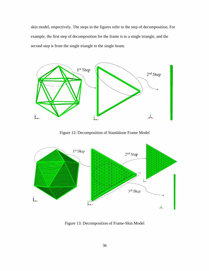
skin model, respectively. The steps in the figures refer to the step of decomposition. For
example, the first step of decomposition for the frame is to a single triangle, and the
second step is from the single triangle to the single beam.
Figure 12: Decomposition of Standalone Frame Model
Figure 13: Decomposition of Frame-Skin Model

37
Table 2 through Table 5 show the natural frequencies calculated for the entire frame,
and frame-skin icosahedron models, as well as the individual components the model is
comprised of. All of the values shown in the tables are in units of Hertz. Table 2
corresponds to the first step in Figure 12 and Table 3 corresponds to the second step
shown in Figure 12. Similarly, Table 4 corresponds to the first step shown in Figure 13,
while Table 5 corresponds to the second step of the icosahedron structure decomposition
as shown in Figure 13. Step three of Figure 13 is not shown in any table because it is the
same beam of the frame, and has equivalent eigenvalues. In each step of the
decomposition, the natural frequencies of the component being analyzed were determined
for three different boundary conditions: free, simply supported, and clamped at the vertex
of the triangle or end of the beam. The three different boundary conditions were applied
in an attempt to characterize the interaction at the vertices of the icosahedron to the
individual triangles, and an illustration of the boundary conditions is shown in Figure 14.
The two dimensional depiction explains the difference between a clamped boundary
condition and a simply supported boundary condition, as they are applied to an individual
beam. The rigid body modes that arise from the free boundary condition placed on the
icosahedron, and occur for natural frequencies of zero, are not shown in the tables.

38
Table 2: Eigenvalues for Icosahedron Frame Decomposition – Triangle
Mode
# Frame
Single Triangle
of Frame – Free
Single Triangle of
Frame – Simply
Supported
Single Triangle of
Frame – Clamped
1 1022.02 1310.01 822.12 1857.08
2 1022.02 1310.01 1035.65 1857.08
3 1022.04 1344.22 1035.65 1857.08
4 1022.04 1344.22 1052.87 1857.08
5 1049.94 1855.95 1052.87 1857.09
6 1049.95 1859.88 1857.09 1857.09
7 1049.95 3841.60 3266.98 5087.01
8 1049.97 3917.15 3266.99 5087.01
9 1049.97 4547.76 3278.12 5087.01
10 1096.96 4547.77 3841.60 5087.01
11 1096.96 4550.54 4562.84 5087.03
12 1096.97 4550.55 4562.85 5087.03
13 1178.22 8219.36 7314.85 9890.33
14 1178.22 8219.37 7497.42 9890.33
15
Rigid Body Modes Omitted
7497.44 9890.33
16 7988.77 9890.33
17 7988.79 9890.37
18 9890.34 9890.37
19 12711.40 16181.90
20 12711.50 16181.90
Table 3: Eigenvalues for Icosahedron Frame Decomposition – Beam
Mode
# Frame
Single Beam of
Frame – Free
Single Beam of Frame –
Simply Supported
Single Beam of
Frame – Clamped
1 1022.02 1863.35 822.80 1858.25
2 1022.02 1863.35 822.80 1858.25
3 1022.04 5116.93 3280.87 5093.55
4 1022.04 5116.93 3280.87 5093.55
5 1049.94 9986.21 7349.31 9923.51
6 1049.95 9986.21 7349.31 9923.51
7 1049.95 16439.90 13004.90 16310.70
8 1049.97 16439.90 13004.90 16310.70
9 1049.97 24499.90 20247.60 24273.40

39
10 1096.96 24499.90 20247.60 24273.40
11 1096.96 26043.30 26043.30 26043.30
12 1096.97 34243.70 29122.70 33889.60
13 1178.22 34243.70 29122.70 33889.60
14 1178.22 40008.40 45326.90 40008.40
15
Rigid Body Modes Omitted
39739.60 45326.90
16 39739.60 52091.70
17 40008.40 58904.10
18 52091.70 58904.10
19 52284.90 75837.00
20 75837.00
Table 4: Eigenvalues for Icosahedron Frame and Skin Decomposition – Triangle with
Beams and Skin
Mode
# Icosahedron
Single Triangle of
Icosahedron –
Free
Single Triangle of
Icosahedron –
Simply Supported
Single Triangle of
Icosahedron –
Clamped
1 18.22 14.80 13.51 13.51
2 18.50 49.71 48.04 48.04
3 18.89 54.91 52.67 52.68
4 19.20 57.36 55.85 55.86
5 19.69 134.22 133.03 133.06
6 19.97 136.96 135.28 135.31
7 20.02 140.61 140.14 140.18
8 28.75 158.65 156.76 156.77
9 29.00 176.67 174.88 174.89
10 30.15 270.00 268.25 268.38
11 31.30 331.61 331.50 331.56
12 33.84 352.84 350.67 350.78
13 34.73 391.68 389.42 389.58
14 35.57 406.48 406.38 406.58
15
Rigid Body Modes Omitted
432.49 432.77
16 487.61 488.51
17 499.39 499.86
18 720.25 722.22
19 795.36 795.79
20 802.42 861.54

40
Table 5: Eigenvalues for Icosahedron Frame and Skin Decomposition – Triangle Skin
Mode
# Icosahedron
Single Triangle of
Icosahedron
(Skin Only) –
Free
Single Triangle of
Icosahedron (Skin
Only) – Simply
Supported
Single Triangle of
Icosahedron (Skin
Only) – Clamped
1 18.22 9.17 2.23 3.23
2 18.50 10.63 5.84 9.26
3 18.89 10.66 5.85 9.37
4 19.20 24.53 15.34 21.50
5 19.69 24.58 15.36 22.02
6 19.97 32.93 20.89 24.49
7 20.02 47.16 38.08 39.74
8 28.75 52.30 38.30 46.23
9 29.00 53.20 38.56 46.76
10 30.15 53.76 52.74 64.83
11 31.30 80.01 65.04 75.90
12 33.84 80.80 65.28 76.58
13 34.73 92.63 68.89 77.82
14 35.57 120.58 105.22 110.87
15
Rigid Body Modes Omitted
105.47 120.32
16 106.52 121.17
17 125.90 132.94
18 153.19 166.94
19 155.29 174.26
20 156.29 175.83
The decomposition of the icosahedron into its components shows a relationship
between each of the individual parts that make up the icosahedron and the entire structure
itself. In almost every case of decomposition, the natural calculated for the individual part
being analyzed are not exactly the same as the entire structure, regardless of the boundary
condition applied. However, for most of the decomposition cases, the first natural
frequency of the entire structure typically lies between the first natural frequency of the
individual parts for the simply supported and clamped boundary conditions. Higher order
modes quickly diverge because the icosahedron has twenty sides, and therefore, has
repeated eigenvalues for the first twenty modes. This relationship of the natural

41
frequencies is intuitive because the vertices of the icosahedron are not rigidly supported,
but they do restrict the motion of the individual components more than a simply
supported boundary condition. Therefore, the vertices of the icosahedron likely present a
boundary condition that lies between the clamped condition and the simply supported
condition. To replicate the boundary condition presented by the vertices of the
icosahedron, a modified clamped boundary condition was devised and tested.
Experimental Test Setup
The construction and testing of an icosahedron is a difficult challenge; however, the
construction of its components is significantly easier. Based on the decomposition study
of the icosahedron, a single triangle of the structure has natural frequencies that lie
between a clamped structure and a simply supported structure at each of the vertices. In
reality, boundary conditions often lie between a simply supported condition and a
clamped condition as “perfect” boundary conditions are impossible to implement.
To achieve a boundary condition stiffer than a pinned end, and softer than a clamped
end, translational and rotational springs can be applied to the end to be more indicative of
the true boundary condition. Figure 14 shows this application for a single beam with only
three degrees of freedom. In the case of the experimental triangle, all six degrees of
freedom are considered. Additionally, an elastic foundation can be applied to an entire
surface if that surface is not rigidly tied to the surface upon which it sits, as shown in the
bottom of Figure 14.

42
Figure 14: Illustration of Pseudo-clamped Boundary Condition and Elastic Foundation
An experimental design had to imitate the boundary conditions of the vertices of the
icosahedron. To produce a boundary condition that lies between the clamped condition
and the simply supported condition, support blocks were constructed at each vertex of the
triangle. The support blocks have a mass significantly larger than the beams of the
triangle, and act as a pseudo-clamped boundary condition. However, the blocks are free

43
to move so the behavior of the frame is representative of the triangle that is part of the
icosahedron structure. Figure 15 shows the Abaqus representation of the experimental
triangle designed to replicate one of the triangles of the icosahedron.
Figure 15: Abaqus Representation of Experimental Test Specimen without Membrane
(Left) and with Membrane (Right)
At the base of the support blocks, translational and rotational springs were applied as
described in the beginning of the section to replicate the pseudo-clamped boundary
condition, and the interaction between the test base and the blocks. In an iterative process
of testing the triangle and modeling it in Abaqus, values for the spring stiffness’s were
determined based on the rigid body mode natural frequencies. An elastic foundation was
utilized in Abaqus on the bottom surface of the support blocks to act as the connection
with the speaker upon which it was tested. The stiffness per area best representative of
the speaker was 1.27 MPa. Additionally, rotational and translational springs were applied
to the center node of the bottom surface to represent the correct interaction. The stiffness

44
of these springs was determined to be 6.8 KPa each. With all of the springs applied to the
experimental triangle model, the natural frequencies and mode shapes of the rigid body
motion matched with good accuracy as can be seen in the results of Chapter IV. As with
the baseline icosahedron model, the beams were modeled using B32 elements, and the
membrane was modeled using the S3R elements. Also, the block supports were modeled
using a solid 20 node quadratic element designated C3D20R. A total of 1914 elements
were used, with 54 elements used for the beams, 324 elements used for the skin, and
1536 elements used for the solid blocks.
A 3-dimensional printer was used to build the experimental triangle and the printing
material was VeroBlue plastic. The skin material used to replicate the membrane of the
baseline model was Kapton tape. The experimental triangle had three major differences
from a single triangle of the previously discussed icosahedron model analyzed in Abaqus:
dimensionality, material properties, and beam cross-section. The dimensions of the
experimental triangle were constrained by the test setup and the capability of the 3-D
printer. To determine the experimental triangle eigenvalues, an input force had to be
applied to the structure, and the method chosen was a standard 6-inch speaker. The
support blocks of the experimental triangle had to set on the lip of the speaker, and
therefore the experimental triangle had to be smaller in dimension than the baseline
icosahedron triangle model. Additionally, the 3-D printer could not print a hollow beam,
such as the beam of the baseline model, without risking damage to the structure.
Therefore, instead of a hollow beam, the experimental triangle had solid beams. Finally,
the material used in constructing the experimental triangle was VeroBlue plastic, rather
than the Beryllium used in the baseline FEA model. These three major differences did not

45
change the modal characteristics of the experimental model because the determining
factor driving the natural frequencies for the structure is its basic geometric properties,
such as long slender beams and an equilateral triangular frame, which was preserved. The
dimensions of the experimental triangle and the material properties are listed in Table 6
below.
Table 6: Experimental Triangle Dimensionality
Dimension Units
Block Support (Height,
Width, and Length) 1.1515 (0.02925) in (m)
Beam Length 3.5335 (0.08975) in (m)
Beam Radius 0.114 (2.9e-03) in (m)
VeraBlue Density 0.043 (1190.0) lb/in³ (kg/m³)
VeraBlue Modulus of
Elasticity ~362594.3 (~2.50) lb/in² (GPa)
VeraBlue Poisson’s Ratio 0.35 (est.) unit less
Kapton Thickness 0.0059 (1.5e-04) in (m)
Kapton Density 0.0513 (1420) lb/in³ (kg/m³)
Kapton Modulus of
Elasticity 362594.3 (2.5) lb/in² (GPa)
Kapton Poisson’s Ratio 0.34 unit less
A standard 6-inch speaker was used to apply a force on the structure, and a laser
vibrometer was used to detect the vibration response of the structure due to the input
force. Figure 16 displays the entire experimental setup with the test specimen placed

46
below the laser vibrometer, and the computer hardware utilized to analyze the signal to
the left. The vibrometer hardware and software used was manufactured by Polytec.
Specifically, the Polytec hardware models for the controller, junction box, scanning head,
and PC were: OFV-5000, PSV-E-401, PSV-I-400, and PSV-W-401, respectively. The
Polytec software used was version 8.8. Figure 17 shows a closer view of the frame only
experimental triangle as well as the frame-skin experimental triangle setup. A periodic
chirp signal was input into the speaker at ±2 Volts from 0-2000 Hertz for the frame, and
from 0-500 Hertz for the frame-membrane. The Polytec theory manual states,
Periodic Chirp is designed to excite all FFT (Fast Fourier Transform) lines of the
measured spectrum. The time signal is generated out of the spectrum by an inverse
Fourier transformation. Typically the magnitude is set for all frequencies to the same
value. The phase is generated by an algorithm which maximizes the energy for a
given maximum amplitude.
After waiting for steady state conditions the excitation and the response are
measured without leakage effects. As all frequencies of interest are excited
simultaneously no averaging is required. This is very useful in order to do fast
measurements. However, for precise measurements averaging can be used in order to
increase the signal-to-noise ratio [26].
Ten averages of displacement were taken at each point to reduce the signal-to-noise
ratio using a sample time of 3.2 seconds for the frame, and 6.4 seconds for the frame-skin
model in constructing the frequency response plot.

47
Figure 16: Experimental Setup
Figure 17: Test Specimen – Frame Only (Left) and Frame-Skin (Right)

48
The process of obtaining the eigenvalues and eigenvectors of the experimental setup
is shown in Figure 18. First, the model was created using the Solidworks Computer
Aided Design (CAD) software and the 3-D printer. Next, the experiment was setup using
the Polytec software, and measurement points were selected for analysis. A periodic chirp
signal was input into the speaker, and the laser vibrometer measured the displacement of
the selected points on the experimental triangle. The input signal to the speaker and the
output signal from the laser vibrometer are analyzed by the software through a Fast
Fourier Transform, and the frequency response plot was developed. Additionally, the
eigenvectors are displayed by the Polytec software. Results of this process are shown in
the following chapter.
Figure 18: Experimental Analysis Process

49
Equivalent Stiffness Study
In addition to decomposing the icosahedron into individual parts, a comparison was
made to a simple beam structure using an equivalent stiffness to characterize the dynamic
behavior of the icosahedron model. This comparison was made to identify similarities to
structures with known dynamical behavior, similar to the decomposition of the
icosahedron. If similarities could be identified then experiments could be carried out
using the simplified model to obtain information on the behavior that would be present in
the icosahedron design.
Figure 19 depicts the process of which the comparison of a complex structure can be
compared to a simple beam through an equivalent stiffness. Abaqus was used to impart
an initial displacement (D) on the icosahedron structure and obtain the reaction force
( ). In a static analysis, force is equal to stiffness multiplied by displacement, or
= KD (refer to Equation (9)). With the force and displacement known, stiffness can
be calculated. To compare the stiffness of the icosahedron to a simple beam, the known
stiffness equation for a beam was utilized. To ensure dynamic similarities, the mass of the
icosahedron frame and the equivalent stiffness beam had to be equal as well. Holding the
stiffness and mass equal allows for the solution of the beam dimensions and the
development of a beam model that can be analyzed.

50
Figure 19: Equivalent Stiffness Comparison Process
The dimensions of the beam with equivalent stiffness and mass to the icosahedron
were computed to be 0.3313 meters in length, and 0.0018 meters for the cross-sectional
radius. Table 7 shows the natural frequencies calculated for both the simply supported,
and the clamped boundary conditions. All values are in units of Hertz. The difference
between some of the natural frequencies calculated for the icosahedron frame and for the
equivalent stiffness beam is relatively small for certain modes (1.5% error between mode
5 of the clamped frame and the clamped beam). However, the mode shapes associated
with those eigenvalues reveal no similarity between the two structures as shown in Figure
20. The first bending mode of the clamped icosahedron frame and the clamped beam
have similar mode shapes, as shown in Figure 21, but the eigenvalue is off by 25.8%. The
comparison between the icosahedron frame natural frequencies and those of the
equivalent stiffness beam did not reveal a relationship strong enough to consider further
diagnosis.

51
Table 7: Natural Frequencies for Equivalent Stiffness Beam
Mode Icosahedron -
Clamped
Beam -
Clamped
Icosahedron - Simply
Supported
Beam - Simply
Supported
1 47.03 59.17 0.00 0.00
2 47.03 59.17 1021.90 166.08
3 83.94 370.68 1021.95 166.08
4 1021.90 370.68 1021.97 664.07
5 1021.97 1037.28 1022.09 664.07
6 1033.62 1037.28 1049.73 1493.16
7 1033.71 2030.85 1049.83 1493.16
8 1048.28 2030.85 1050.07 2652.03
9 1049.73 3353.30 1050.16 2652.03
10 1049.83 3353.30 1053.25 4138.86
11 1096.76 5002.23 1096.76 4138.86
12 1096.87 5002.23 1096.86 5951.37
13 1128.24 6295.90 1097.12 5951.37
14 1162.04 6975.07 1177.59 8086.82
15 1162.07 6975.07 1177.63 8086.82
16 1178.18 9268.81 1178.18 10542.10
17 1178.22 9268.81 1178.22 10542.10
18 1215.03 9671.95 1178.72 12591.80
19 1215.04 11880.00 1304.00 13313.60
20 1232.33 11880.00 1314.99 13313.60
The equivalent stiffness study was conducted as an alternative way to develop a
reduced order volume that could be built and tested in lieu of the entire icosahedron. The
decomposition of the icosahedron model into its individual parts revealed strong
similarities between the single face of the icosahedron and the structure as a whole.
However, the equivalent stiffness method was determined to be non representative of the
entire icosahedron.

52
Figure 20: Mode Shape Difference for Icosahedron Frame and Equivalent Stiffness Beam
Figure 21: Similar Mode Shapes for Icosahedron Frame and Equivalent Stiffness Beam
53
Time Step Study
A complete dynamic analysis using FEA requires a sufficient number of elements in
the model, the correct type of elements for the structure, and the appropriate integration
time step size for calculating the solution. The type of elements used, and the number
necessary to calculate an accurate solution was presented in previous sections. This
section establishes the time step required for calculating the solution. Referring to
Equation (14), the numeric solution to the structural analysis problem is dependent upon
the size of the time step. If the specified time step is too large a solution may be
indeterminable, or inaccurate.
A common method used to select the correct time step is to obtain the displacement
results for varying time steps, and utilize the power spectral density function to analyze
the eigenvalues admitted from the solution. In this research, the time step variation
analysis was executed using a single beam of the icosahedron discretized into eight B32
beam elements. Simple supports at each end were the boundary conditions for the beam,
and an initial displacement of ~0.6% of the length of the beam was placed at the quarter
beam position. The initial displacement was chosen so the response would remain in the
linear range. The nonlinear solution option was selected in Abaqus, although the same
results would have been obtained if a linear response was requested, because of the size
of the initial displacement. The initial displacement was removed and the free response of
the beam as a function of time was generated using Abaqus. This simple problem allowed
for a comparison to the analytical values of the eigenvalues found in the literature. Figure
22 displays the simple beam setup input to Abaqus, and Table 8 shows the beam natural
frequencies calculated analytically, and through FEA using Abaqus.

54
Figure 22: Boundary Conditions and Initial Displacement for Time Step Study
Table 8: Analytical and Abaqus Calculated Natural Frequencies for Simple Beam
Mode# Analytical Abaqus %Error
1 824.0 822.83 0.14
2 3296.02 3282.34 0.42
3 7416.04 7365.15 0.69
4 13184.08 13088.0 0.73
5 20600.12 20541.3 0.29
Table 9 shows the beam natural frequencies calculated using the PSD method. The
accuracy of the calculated eigenvalues clearly increases as the time step decreases, with
less than one percent error calculated for all natural frequencies using a time step of 1e-6
seconds. Using a time step of 1e-5 seconds produces the first three eigenvalues with an
error of less than 2.5%, although the accuracy declines at the higher number modes. The
fifth natural frequency calculated using a time step of 1e-5 seconds has an error of 12.3%.
Error percentages for both Table 8 and Table 9 were calculated based on the analytical
values. Eigenvalues are not presented in Table 9 for the fourth mode because of the
location which the displacement data was analyzed, called the reference point. The

55
reference point in this case is the quarter beam position, and the fourth mode shape has a
node directly at that point. As Avitabile states in Experimental Modal Analysis, “the
reference point cannot be located at the node of a mode otherwise that mode will not be
seen in the frequency response function measurements and the mode cannot be obtained”
[18].
Table 9: PSD Calculated Natural Frequencies for Simple Beam
Mode# dt = 1e-4 s dt = 5e-5 s dt = 1e-5 s dt = 5e-6 s dt = 1e-6 s %Error
1 801.78 823.1 822.41 822.31 822.24 0.21
2 2516.7 3003.3 3267.4 3289.3 3288.96 0.21
3 3608.02 5250.3 7223.8 7334.15 7355.7 0.81
4 Undetected Undetected Undetected Undetected Undetected N/A
5 Undetected Undetected 18048.5 19780.0 20511.6 0.43
Displacement plots for the various time step values are shown in Figure 23 and Figure
24. Table 9 showed the solutions dependence on choice of time step in the accuracy of
the response. The displacement plots also show the importance of selecting a proper time
step. Larger value time steps result in inaccurate data that decrease in amplitude over the
course of the simulation. The displacement plot in Figure 24 shows that a time step of 1e-
5 seconds or less produces an almost identical response. Figure 25 and Figure 26 show
the PSD plots as a function of decreasing time step. These plots clearly show a certain
time step is required for an accurate solution; too large of time step leads to displacement
plots not representative of the correct response, and the values of the natural frequencies
obtained by the PSD plots vary by significant amounts, or do not appear at all.
Additionally, Figure 25 shows the PSD plot is cut off before a frequency of interest (20
kHz) because of the lack of data points.

56
Figure 23: Displacement versus Time for First Four Time Step Values
Figure 24: Displacement versus Time for Last Three Time Step Values

57
Figure 25: PSD for Time Step of 1e-4 seconds
Figure 26: PSD for Time Step of 1e-6 Seconds

58
Some error can be expected in running computer simulations because the Abaqus
dynamic/implicit solver “generally introduces some degree of numerical damping” that
could be responsible for the difference in natural frequency determined using the power
spectral density [17]. Further decreasing the time step value would likely lead to more
accurate results; however, a significant amount of computational power and memory is
required to decrease the value more than 1e-6 seconds and will not be done for this
research as a percentage error of less than one percent was considered sufficient. In most
cases, only the first few natural frequencies and mode shapes are compared to determine
similarities. Therefore, a time step value of 1e-5 seconds or less was used for the
remainder of the analysis in this thesis.
Summary
This chapter presented the development of a dynamic model starting with the baseline
model originally developed by Adorno-Rodriguez for a static analysis. The icosahedron
was decomposed into its individual parts to simplify the structure, and obtain a
representable model that could be used in experiments because the full is challenging to
construct. An experimental setup was detailed as an attempt to verify the accuracy of the
solutions obtained using the Abaqus FEA program. Additionally, an equivalent stiffness
method was discussed to simplify the complex icosahedron into a well-understood
structure. Finally, the time step necessary for a dynamic analysis was considered to
ensure the accuracy of the model.

59
IV. Analysis and Results
Chapter Overview
Modeling techniques for analyzing the icosahedron structure dynamically were
detailed in the previous chapter as well as a method for verifying the computer model
experimentally. This chapter will describe the results of those methods as they were
applied, and consider the relevance of the information in terms of three basic questions:
Can a simplified model be created to test a representable structure in reality?
At what applied load and load rate do the response characteristics of the
structure become dominated by dynamics?
What is the behavior of the structure when subjected to dynamical loading for
various boundary conditions?
The results of the experimental tests are presented along with comparisons to the
related computer models in the first section. Next, an analysis of the loading rate is
considered in order to impart a dynamic response. Finally, various loading scenarios are
developed and the behavior of the response is characterized.
Experimental Results
Given the relationship between the icosahedron frame and the frame-skin models to
the single triangle of the icosahedron, an experimental setup was created to test a
representable volume in an effort to validate the FEA model that has been the basis of the
research. The experimental setup was explained in detail in the previous chapter, and the
results are provided in this chapter.

60
The results of decomposing the icosahedron into its individual parts and analyzing the
natural frequencies and mode shapes of each component using various boundary
conditions led to an experimental triangle that was explained previously. In an iterative
process, the experimental triangle was created, tested, and the FEA model was updated to
reflect the results of the testing. A final FEA model was developed matching the first
several mode shapes and natural frequencies of the test specimen. Figure 27 displays the
first six mode shapes observed in testing calculated by Abaqus. Only the relevant modes
are displayed, related to the speaker’s vertical translation input force.
Figure 27: Modes 1 through 6 – FEA Experimental Triangle (Frame)

61
Figure 28 shows the points of measurement for the experimental triangle setup, as
well as the view seen from the laser vibrometer position. As the drive signal is input to
the speaker, the vibrometer measures displacement at each point over a number of
periods of the input signal. The software takes the average output movement of the
triangle and creates a frequency response plot for the entire structure. The mode shapes of
the experimental triangle are shown in Figure 29, and the frequency response plot is
shown in Figure 30. In Figure 29, the top picture for each natural frequency is the
movement as the triangle beams move away from the speaker, while the bottom picture is
the movement into the speaker to show the full range of motion at a given frequency. The
black dots in Figure 29 represent the initial point on the structure before any
displacement, and the color of the squares represent the distance from the original
position. Red is the greatest positive distance from the reference point, and blue is the
greatest negative distance from the reference position. The color graduated bars in
between the extremes mirrors the scale used by the FEA plots shown in Figure 27.
Figure 28: Points of Measurement for Experimental Triangle

62
Mode #1: 29.6875 Hz Mode #2: 97.1875 Hz
Mode #3: 464.0625 Hz Mode #5: 1280.938 Hz
Figure 29: Experimental Triangle Mode Shapes and Natural Frequencies (Frame)
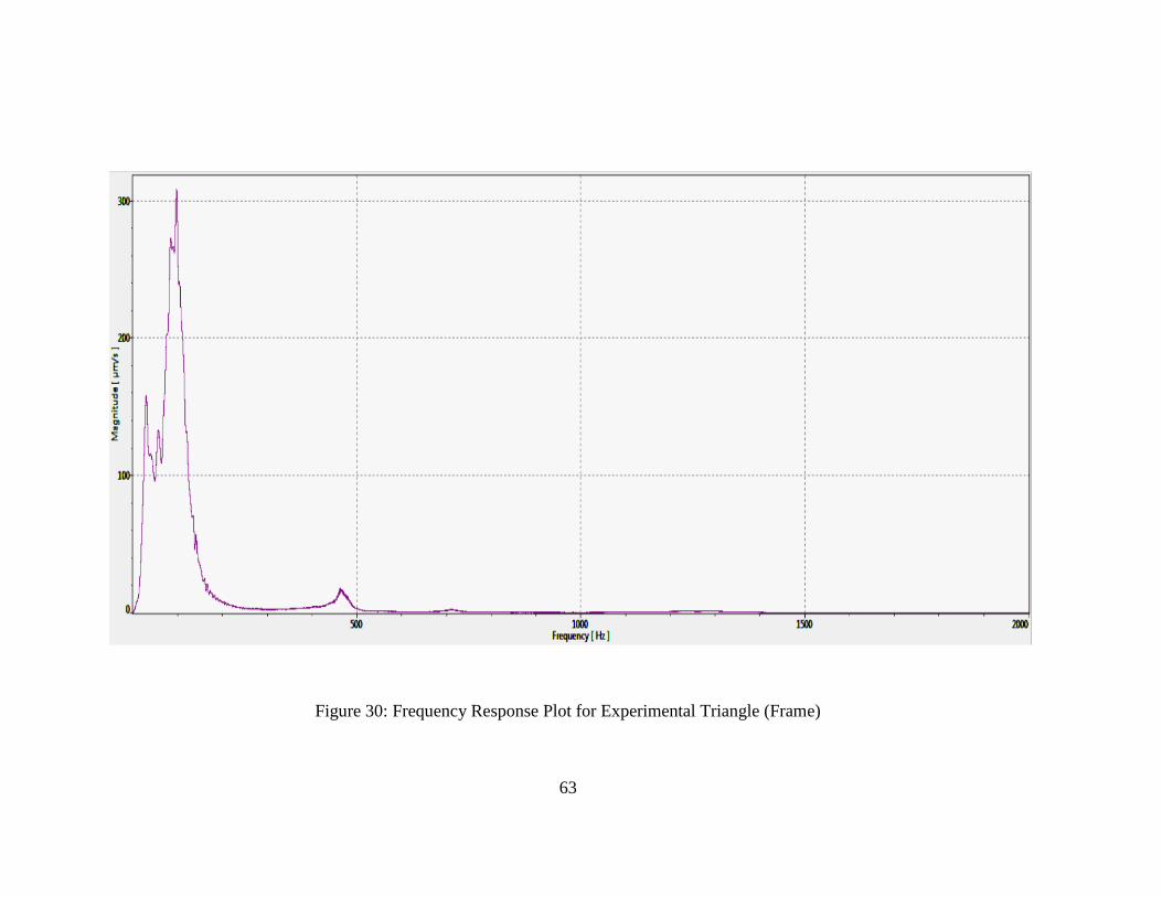
63
Figure 30: Frequency Response Plot for Experimental Triangle (Frame)

64
A variety of factors impacted the accuracy of the results obtained from this
experiment, including noise and input signal parameters. Variations on the parameters did
not have a large effect on the natural frequencies and mode shapes detected by the laser
vibrometer, but there was some difference. Using ten averages at each point reduced the
effect of noise; however, it cannot be eliminated. The experimental triangle and the FEA
triangle produced very similar natural frequencies and mode shapes with the exception of
the fifth mode shown in Figure 27. The first bending mode (491 Hz) of the frame beam
was not detected in the experiment. A likely explanation for the lack of detection of the
first bending mode is the difference between natural frequencies and operating deflection
shapes arising from the experimental data. Operating deflection shapes are the mode
shapes that are determined given all of the outlying circumstances. In a perfect
experiment the operating deflection shapes would be the same as the true mode shapes.
Factors such as noise, input parameters, and modal coupling can cause differences
between the two. The first bending mode of the frame beams (mode 5 shown in Figure
27) lies very close to the mode before it, where two beams bend in opposite direction
while the third beam remains nearly stationary. In the experimental setup there could be
coupling between these modes and there could be a lack of input signal necessary to
generate the mode described as the first bending of the frame beam.
In addition to comparing the experimental triangle with the FEA triangle, a
reconstruction of the entire icosahedron frame was conducted to determine if the
experimental triangle was truly representative of the whole icosahedron frame. The
icosahedron frame was reconstructed in Abaqus using the material properties of the 3-D
printer material and the geometric dimensions were the same as the triangle. Table 10

65
displays the related eigenvalues of each model in Hertz. The first two rows of the table
show the rigid body modes (RBM) that are associated with the speaker setup and
therefore undetected on the icosahedron frame model.
Table 10: Natural Frequencies of FEA Experimental Triangle Frame, Experimental
Triangle Frame, and FEA Icosahedron Frame
Mode
#
Icosahedron
Frame
Experimental Triangle
Frame - Abaqus
Experimental Triangle
Frame - Vibrometer
RBM 0.0 30.0418 29.6875
RBM 0.0 97.4186 97.1875
1 400.47 469.6590 464.0625
2 457.21 491.3780 Undetected
3 1260.000 1266.4200 1280.938
The information contained in Figure 27, Figure 29, and Table 10 demonstrates a
strong relationship between the FEA experimental triangle model, the real experimental
triangle, and the icosahedron frame they were designed to replicate. Figure 31 displays
the mode shapes of the entire icosahedron frame, and a single triangle of the frame has
the same mode shapes as the experimental triangle models of Figure 27 and Figure 29.
The natural frequencies of the three designs varies by at most 16% from the icosahedron
frame to the experimental triangle for the first mode; however, this difference can be
explained by the various factors affecting the model as detailed earlier, and more
accuracy could be achieved with a more rigorous test setup and model construction.
Additionally, more accurate material properties may need to be applied to the FEA model
to achieve less error between the Abaqus results and the experimental setup.
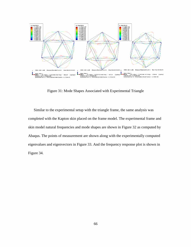
66
Figure 31: Mode Shapes Associated with Experimental Triangle
Similar to the experimental setup with the triangle frame, the same analysis was
completed with the Kapton skin placed on the frame model. The experimental frame and
skin model natural frequencies and mode shapes are shown in Figure 32 as computed by
Abaqus. The points of measurement are shown along with the experimentally computed
eigenvalues and eigenvectors in Figure 33. And the frequency response plot is shown in
Figure 34.

67
Figure 32: Modes 1 through 8 – FEA Experimental Triangle (Frame-Skin)

68
Measurement Points – Experimental
Triangle with Skin Mode #1: 36.25 Hz
Mode #2: 122.03125 Hz Mode #3: 216.5625 Hz

69
Mode #4: 240.9375 Hz Mode #5: 361.5625 Hz
Mode #6: 380.46875 Hz Mode #7: 472.34375 Hz
Figure 33: Experimental Triangle Mode Shapes and Natural Frequencies (Frame-Skin)

70
Figure 34: Frequency Response Plot for Experimental Triangle (Frame-Skin)

71
Table 11 lists the natural frequencies associated with the FEA experimental triangle
with skin, true experimental triangle, and the icosahedron with skin. Figure 35 displays
the mode shapes of the icosahedron. As with the frame only model, the relationship
between the experimentally calculated operating deflection shapes and those of the FEA
models is strong. Eigenvalues detected in the experimental analysis are shown in the FEA
triangle and the icosahedron model as well, and the mode shapes associated are
comparable between all three. Results of the experimental analysis imply a single triangle
of the icosahedron is representable of the entire structure, and the modeling techniques
used are accurate.
Table 11: Eigenvalues of FEA Experimental Triangle Frame, Experimental Triangle
Frame, and FEA Icosahedron Frame
Mode
#
Icosahedron Experimental Triangle
Frame and Skin - Abaqus
Experimental Triangle Frame
and Skin - Vibrometer
RBM 0.0 29.9113 36.25
RBM 0.0 92.4764 Undetected
1 125.667 127.3380 122.03125
2 252.141 246.7550 216.5625
3 261.387 254.2790 240.9375
4 Undetected Undetected 361.5625
5 411.452 390.3720 380.46875
6 478.173 423.3630 472.34375

72
Figure 35: Mode Shapes Associated with Experimental Triangle with Skin
Chaotic Behavior Analysis
In addition to validating the baseline model developed in previous research, a
dynamic analysis of the icosahedron frame snapback behavior reported by Adorno-
Rodriguez is conducted to identify nonlinear instability characteristics of the design.
Adorno-Rodriguez compares the snapback behavior to the buckling of a thin shell, where
an instantaneous reversal of geometry occurs, but the structure retains a load-bearing
capacity. In the previously mentioned research, the behavior was observed for two of the
boundary conditions considered. Figure 36 shows the different boundary conditions
considered, and the snapback behavior seen in the first and second boundary conditions
for the static loading case. This behavior “indicates a beam withdrawal, or change in
displacement direction, while still taking on load. Even though the slope reverses, there is

73
no softening, therefore the beam does not collapse” [7]. The results are hypothesized to
be chaotic behavior present in the standalone frame model. To validate the theory of
chaotic behavior in the icosahedron frame, a dynamic analysis is performed and the
methods described in Chapter II are applied.

74
Figure 36: Snapback Behavior Observed in Unsymmetrical Boundary Conditions [7]
15
0 .5
100 200 300 400 500 600 Edge Midpoint Umaon'\.eam
(a) Boundary Condition 1
4 6
4 55
1.5 4 .5
4 .4S '='550=------=600=-----=6=50=----,7=oo-=-----=750:::----'
200 400 600 800 1000 1200 1400 Edge Midpoint Umaon'\.eam
(b) Boundary Condition 2
10
4
0 500 1000 1500 2000 2500
(c) Boundary Condition 3

75
Load Rate Analysis
One consideration necessary with a dynamic analysis, but not a static analysis, is the
rate which a load is applied. In the case of a static analysis, the load is applied in a
manner in which the structure is held in equilibrium and acceleration is equal to zero. A
dynamic response will appear similar to the static response if the load is applied at a slow
rate. Therefore, to evaluate the rate which a reasonable dynamic response could be
produced and to define the line between dynamic and static loading, an analysis of
ramped loads was considered.
The snapback behavior can be seen to occur at approximately 45% of Sea Level
pressure (~45 kPa) for what is called “Boundary Condition 1” (BC1) and “Boundary
Condition 2” (BC2) in the plot of the applied load versus displacement of Figure 36 [7].
“Boundary Condition 3” (BC3) does not display the same behavior at any point up to
100% of Sea Level pressure. Figure 37 shows BC3 and the loading applied to the
icosahedron frame through reference points at the center of gravity of each triangle, as
well as the midpoint node on the lower beam where all displacement data is collected.
The midpoint node was used because the icosahedron deforms symmetrically, and all
midpoint nodes on all beams have equivalent displacement. Also, it is the reference point
referred to in previous research, and has the greatest displacement of any node on the
structure. The concentrated load applied to the reference points was distributed to the
beams using a coupling constraint in Abaqus. The coupling constraint allows the beams
to experience an equivalent load to one that would be applied if a triangular skin with an
applied pressure was tied along the edges. Adorno-Rodriguez conducted a study to ensure

76
the applied load experienced by the beams was identical using the reference point and
coupling constraint method, or using a skin tied to the beams [7].
Figure 37: Boundary Condition and Load Applied for Load Study
Figure 37 shows the top and bottom nodes are restricted in the x and y direction,
while all other degrees of freedom are free to move. The simple difference between BC3
and BC2 is all degrees of freedom are constrained at the bottom node in BC2 instead of
only the x and y directions. BC1 has all degrees of freedom restricted at the bottom node,
but none restricted at the top. BC3 was found to respond to the statically applied pressure
in a symmetric behavior, while the other two boundary conditions produced
nonsymmetrical behavior that led to a sudden change in slope of the applied pressure

77
versus displacement plots shown in Figure 36. The load which an instantaneous change in
displacement direction occurs is referred to as the snapping load. When the load was
applied dynamically, BC3 did not continue to respond in a symmetric fashion, but instead
began spinning about the z-axis when the baseline icosahedron model was used. To
achieve dynamic symmetry, the load at the reference point was changed to a follower
force to replicate a pressure being applied, and eliminate the spinning motion. A follower
force remains normal to the tangent plane of the surface where the load is applied on the
structure. Figure 38 displays a simple example of a follower force applied to a cantilever
beam. By definition, pressure is a follower force.
Figure 38: Follower Force (Left) and Non-follower Force (Right) [7]
The study of chaotic behavior in a system requires a dynamic response dependent on
the initial conditions applied to that system. Previously, boundary conditions and
symmetry were considered. Now, the effect of the rate of loading on the structure is
considered. Various loading scenarios applied to the frame are shown in Figure 39. Each
applied load is in the form of a ramp input, which can be written as r(t) = t*u(t), where

78
u(t) is the step input function. The step input function is equal to unity for time greater
than zero and zero for time less than zero [19]. The displacement response, also known as
the ramp response, to the ramp input function is shown in Figure 40.
Figure 39: Various Loading Conditions for Load Study
Figure 40: Displacement versus Time Curves for Various Loading Conditions

79
As the rate of loading is increased, the difference between the static response and the
dynamic response is shown with more oscillations occurring once the full load is applied.
A rise time of 0.005 seconds, corresponding to a load rate of 4.053 MPa- ˉ¹, sufficiently
displayed the dynamic characteristics of interest in this research. A rate of at least that
value is used for the remainder of this thesis in studying chaotic behavior.
Chaotic behavior is dependent on the initial conditions applied to a system, and the
rates which loads are applied effectively change the initial velocity of the icosahedron
frame, which changes the initial conditions. The initial slopes of the displacement curves
in Figure 40 are the initial velocities, and increasing the initial velocity increases the
oscillations that occur once the full load is applied. This makes sense as the increase in
velocity is directly correlated to an increase in kinetic energy in the system. When the
amount of energy applied to the system is too great for the structure to absorb, a
snapback behavior occurs. However, if too little energy is applied to the system (too
small of initial velocity), the response appears to be the same as the static response and
chaos cannot be examined. The time step used in evaluating the varying loading scenarios
was set to automatic, rather than fixed, for reasons stated in the previous time step study
discussed in Chapter III. Applying the automatic time step in Abaqus allows the program
to select an appropriate time step for that iteration, and it allows the program to change
the time step over the course of solving the problem. The reason for this is a detailed
response was not desired, only a definite point where the response changes from
exhibiting static characteristics to dynamic characteristics, enabling a chaotic motion
analysis.

80
The snapback behavior presented by Adorno-Rodriguez occurred in the first two
boundary conditions that were deemed unsymmetrical. However, the snapping behavior
developed for all boundary conditions, including BC3, when the load was applied
dynamically. Additionally, the load that caused the snapback behavior to occur decreased
when the load was applied dynamically instead of statically, and the value to which it
decreased was dependent on the initial conditions (load rate). The ramp input load
scenarios applied to the frame above the snapping load are shown in Figure 41, and the
displacement versus time ramp response to those loads is shown in Figure 42.
Figure 41: Loads above Snapping Load

81
Figure 42: Displacement versus Time Curves above Snapping Load
The results of the load rate analysis shows the importance of what load is applied, and
at what rate it is applied. These initial conditions drive the dynamics of the system, and
for certain scenarios, lead to chaotic behavior. Clearly, Figure 40 shows the difference
between a slowly applied load and a quickly applied load. The structure exhibits greater
oscillatory behavior as the time over which the load is applied decreases. Also, Figure 42
displays what happens to the structure when the applied load is too large, regardless of
the time over which the load is applied. These results are utilized in studying the chaotic
behavior associated with the frame when an unsymmetrical boundary condition is
applied, or the applied load is too great. Table 12 displays the various loading scenarios
considered, and the boundary conditions of the frame to which they were applied. The
last two load scenarios incorporated the skin with the frame to observe the effect it has on
the instability characteristics of the model.

82
Table 12: Loading Rates for Applied Pressure
Load
#
% of Sea Level
Pressure Applied Ramp Duration (s)
Load Rate
(MPa-sˉ¹)
Boundary
Condition
1 10 0.002 5.0663 BC3 (Frame)
2 20 0.005 4.053 BC3 (Frame)
3 40* 0.005 8.106 BC3 (Frame)
4 10 0.002 5.0663 BC2 (Frame)
5 20 0.005 4.053 BC2 (Frame)
6 40* 0.005 8.106 BC2 (Frame)
7 40 0.005 8.106 BC3 (Frame-skin)
8 60 0.005 12.159 BC3 (Frame-skin)
*Above dynamic snapping load for frame determined for the applied load rate
Icosahedron Frame Boundary Condition Three
In a static analysis, BC3 did not display the snapback behavior present in both BC1
and BC2. This section investigates the effect of dynamic loading on the structure using
the same boundary condition. From Table 12, three dynamic loads are considered in
determining if chaotic motion is present in the design. The first two loads are below the
snapping load, while the third load is above.
For each load number, four plots were generated to determine if chaotic behavior
exists. The first plot is the displacement versus time response for the given load. The
second plot is the phase plane trajectory, displaying velocity versus displacement. The
third plot is the power spectral density plot for the given load, and the fourth plot shows
the convergence of the Lyapunov exponent calculated by Equation (20). Lyapunov
exponent convergence plots were developed using MATLAB code provided by Wolf, et
al., and the methods described in Determining Lyapunov Exponents from a Time Series
article [25]. The MATLAB code is in the Appendix for reference.

83
The method developed by Wolf, et al. creates a delay reconstruction of the attractor
described in Chapter II. It then cycles through the delay reconstructed data and calculates
an estimate for the Lyapunov exponent at each evolution of the data. Delay
reconstructions of the attractor were made using the delay parameter τ, which was varied
in order to avoid producing a crossing or folding of the trajectories within the attractor.
Crossing or folding of trajectories can lead to a false positive Lyapunov exponent. The
algorithm cycles through the trajectory based on a number of input parameter values to
calculate the Lyapunov exponent, as explained by Wolf, et al. [25].
Figure 43 through Figure 55 show the result of load numbers 1 through 3 as they were
applied to the icosahedron frame with BC3. The results for load number 1 are displayed
in Figure 43 through Figure 46. The applied load is well below the static and dynamic
snapping load. As the plots show, the load does not cause a snapback behavior, and
reaches a steady state oscillation which is purely periodic. There is no damping applied to
the model, so the phase plane trajectory remains on a single orbit, rather than decreasing
in size over time. The PSD plot shows the frequency response, and shows a dominant
natural frequency at 1500 Hertz. This value is different than the Abaqus calculated value
shown in Table 2 which lists the first natural frequency occurring around 1022 Hertz.
However, this difference can be attributed to the addition of the load on the structure, and
the change in boundary conditions. Finally, the convergence of the Lyapunov exponent to
a negative number in Figure 46 indicates the response of the icosahedron frame for load
number 1 is non-chaotic.

84
Figure 43: Load 1, BC3, = -0.0121 bits/orbit, Displacement Curve
Figure 44: Load 1, BC3, = -0.0121 bits/orbit, Phase Plane Trajectory

85
Figure 45: Load 1, BC3, = -0.0121 bits/orbit, PSD
Figure 46: Load 1, BC3, = -0.0121 bits/orbit, Lyapunov Exponent Convergence Plot

86
For load number 1, the Lyapunov exponent was calculated using 4500 data points
spaced at 1e-5 second intervals. The initial 0.002 seconds of data corresponding to the
ramped load is omitted from the calculation, as the transient response data is not desired.
The following parameters were used in the MATLAB algorithm (see Wolf, et al.): tau =
8, evolve = 8, dismin = 1e-8 and dismax = 2e-4. Figure 47 shows an example of the
reconstructed attractor for load number 1. As expected, for a purely periodic response,
the attractor is simply a closed curve. The attractor is reconstructed in three dimensions
because the system is three-dimensional, and the plot is made of ordered triples
comprised of the displacement data separated by the delay parameter, τ. For example, one
point has coordinates of [u1(t), u1(t+τ), u1(t+2τ)]. The dismax parameter was selected
based on the longest distance between points in the reconstructed attractor plot, and
dismin was set to be smaller than the shortest distance between points. The tau and evolve
parameters are chosen heuristically so the attractor does not appear to fold on itself
which can lead to a false positive Lyapunov exponent calculation.

87
Figure 47: Delay Reconstructed Attractor for Load 1, BC3, = -0.0121 bits/orbit
Load number 2 leads to the same conclusion as load number 1. The displacement
curve, phase plane trajectory, PSD plot, and Lyapunov convergence are nearly identical
to those of load number 1. Again, there is a periodic steady state oscillation present after
the load is applied resulting in a fixed orbit shown in the phase plane trajectory. The PSD
is smooth and has a clearly identifiable natural frequency, while the Lyapunov exponent
converges to a negative value. The input parameters for the Lyapunov exponent
calculations were the same as those used in load number 1. All of the information
presented indicates non-chaotic behavior.

88
Figure 48: Load 2, BC3, = -0.0137 bits/orbit, Displacement Curve
Figure 49: Load 2, BC3, = -0.0137 bits/orbit, Phase Plane Trajectory

89
Figure 50: Load 2, BC3, = -0.0137 bits/orbit, PSD
Figure 51: Load 2, BC3, = -0.0137 bits/orbit, Lyapunov Exponent Convergence Plot

90
Load number 3 is applied above the snapping load pressure, and presents extremely
different results, both quantitatively and qualitatively. The displacement curve is no
longer purely periodic, but instead seems to vibrate disorderly, and it has amplitude
approximately 100 times that of load number 2. The snapback behavior can be seen as
the displacement instantaneously changing direction. Furthermore, the phase plane
trajectory has no apparent repeated pattern, but does generally remain within an elliptical
envelope. The orbits of the trajectory appear to fill up a portion of the phase space,
indicating chaotic behavior as stated in Chapter II. The frequency response has changed
character from load number 1 and 2, becoming noisy, and not clearly showing a peak
frequency. Finally, the convergence of the Lyapunov exponent is well above zero
bits/orbit, indicating significantly chaotic behavior occurring above the dynamically
applied snapping load. The bits/orbit unit is carried over from Wolf’s information theory
terms, where bits references amount of information. Specifically, “the exponents measure
the rate at which system processes create or destroy information… Hence if an initial
point were specified with an accuracy of one part per million (20 bits), the future
behavior could not be predicted after about” 0.0018 seconds, corresponding to less than
one quarter of a single orbit. “After this time the small uncertainty will essentially cover
the entire attractor, reflecting 20 bits of new information that can be gained from an
additional measurement of the system” [25]. In short, load number 3 displays chaotic
behavior such that after only a quarter of a single orbit predictability is lost.
Values of the input parameters to the algorithm for load number 3 were tau = 80,
evolve = 80, dismin = 1e-8 and dismax = 2e-2. The change is largely attributed to the
change in amplitude in the displacement curve, as well the decrease in time step used in

91
obtaining the solution. As discussed in Chapter III, the time step had to be decreased to
1e-6 seconds for Abaqus to converge on a solution to the problem, instead of the value of
1e-5 seconds used in the simpler problems using load number 1 and 2.
Figure 52: Load 3, BC3, = 3.8814 bits/orbit, Displacement Curve
Figure 53: Load 3, BC3, = 3.8814 bits/orbit, Phase Plane Trajectory

92
Figure 54: Load 3, BC3, = 3.8814 bits/orbit, PSD
Figure 55: Load 3, BC3, = 3.8814 bits/orbit, Lyapunov Exponent Convergence Plot

93
Icosahedron Frame Boundary Condition Two
The same loads applied to BC3 were applied to BC2 to confirm the snapback
behavior originally presented in the static analysis. Figure 56 through Figure 59 show the
results of load number 4, Figure 60 through Figure 63 show the results for load number 5,
and Figure 64 through Figure 67 are from load number 6.
Load 4 and 5 create responses similar in each of the plots analyzed. Figure 56 and
Figure 60 reveal the most periodic displacement curves with small disturbances occurring
throughout the response. The displacement curve of load number 5 grows more erratic,
and the number of non-periodic disturbances increases as the applied load increases. The
phase plane trajectories of the two responses are also similar, settling into an elliptical
orbit of varying size. These variations in the orbit size correspond to the disturbances
shown in the displacement plots. As the force increases in load number 5, the
disturbances become larger and more numerous, which gives rise to larger variations in
the orbits of the phase plane trajectory. The PSD plot of the two loads looks similar, with
peak frequencies at 1556 Hz and 1200 Hz, respectively. However, the increased pressure
of load number 5 is responsible for more peaks being present than in the PSD plot of load
number 4. The Lyapunov exponent convergence plot shown in Figure 59 and Figure 63
share the same characteristics, with the final convergence settling at a slightly positive
number. Returning to the example given in the previous section on the interpretation of
the final value for the Lyapunov exponent, predictability is lost after 65.9 orbits, and
53.95 orbits for load numbers 4 and 5, respectively (assuming 20 bits of “good” data
initially). The input parameters for the Lyapunov exponent code were the same for load

94
number 4 and load number 5; specifically, they were tau = 15, evolve = 10, dismin = 1e-
8 and dismax = 2e-4.
All of the response plots from load number 4 and load number 5 indicate that BC2
presents a slightly chaotic behavior, decreasing in predictability as the load rate is
increased. While the snapback behavior associated with the unsymmetrical boundary
condition is not identified by applying load number 4 or 5, the structure seems to respond
in a chaotic fashion below the dynamically applied snapping load. This indicates small
changes in the initial conditions cause significant changes in the response of the structure
under BC2.
Figure 56: Load 4, BC2, = 0.303 bits/orbit, Displacement Curve
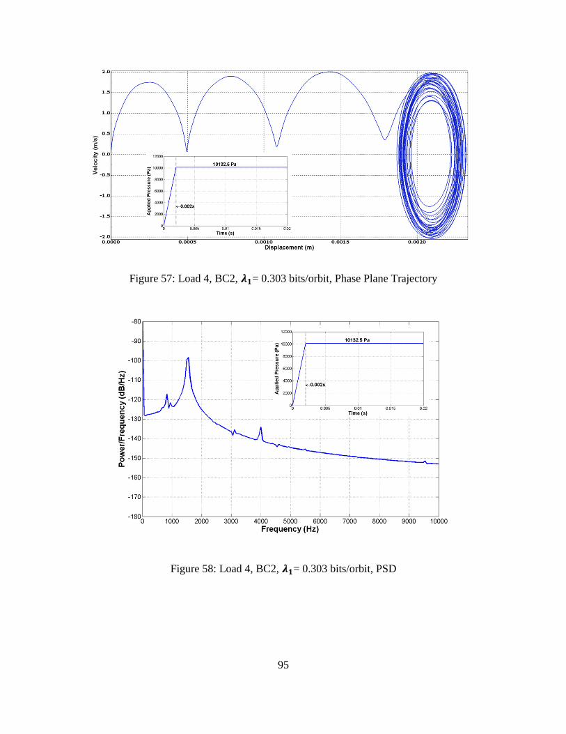
95
Figure 57: Load 4, BC2, = 0.303 bits/orbit, Phase Plane Trajectory
Figure 58: Load 4, BC2, = 0.303 bits/orbit, PSD

96
Figure 59: Load 4, BC2, = 0.303 bits/orbit, Lyapunov Exponent Convergence Plot
Figure 60: Load 5, BC2, = 0.371 bits/orbit, Displacement Curve

97
Figure 61: Load 5, BC2, = 0.371 bits/orbit, Phase Plane Trajectory
Figure 62: Load 5, BC2, = 0.371 bits/orbit, PSD

98
Figure 63: Load 5, BC2, = 0.371 bits/orbit, Lyapunov Exponent Convergence Plot
Load number 6 is applied to BC2 just as load number 3 was applied to BC3. The
dynamically applied load is above the pressure required to create the snapback behavior
for the symmetrical BC3, therefore, it is expected to produce similar, if not more chaotic
results for BC2. Figure 64 through Figure 67 shows the results of the loading scenario,
and show the response is more chaotic than the response to load number 3 applied to
BC3. Specifically, the Lyapunov exponent converges to a significantly higher value for
load number 6, corresponding to lost predictability after a single orbit. The input
parameters for the Lyapunov exponent code were: tau = 150, evolve = 80, dismin = 1e-8
and dismax = 2e-2.

99
Figure 64: Load 6, BC2, = 19.67 bits/orbit, Displacement Curve
Figure 65: Load 6, BC2, = 19.67 bits/orbit, Phase Plane Trajectory

100
Figure 66: Load 6, BC2, = 19.67 bits/orbit, PSD
Figure 67: Load 6, BC2, = 19.67 bits/orbit, Lyapunov Exponent Convergence Plot

101
Icosahedron Frame and Skin Boundary Condition Three
Previous research indicated the frame itself exhibited a snapback behavior. The same
behavior was not predicted to occur when the skin was placed on the frame to create the
full icosahedron LTAV design. However, with the knowledge a dynamic snapping load is
observed below the static load, and the snapback behavior is present in the frame for the
symmetric BC3 when subject to the dynamic load, the dynamic load above the snapping
load was applied to the entire icosahedron model to determine if the snapback occurred.
Figure 68 through Figure 71 represent the response of the full icosahedron LTAV
design to load number 7, which caused the snapback behavior to occur in the frame.
Additionally, Figure 72 through Figure 75 show the response to load number 8, which
reaches 60% SL pressure. Interestingly, both loading scenarios result in very similar
responses which are somewhat different from the responses seen in the frame alone. The
displacement curves shown in Figure 68 and Figure 72 show highly periodic behavior,
even as the load rises to its steady state level. The phase plane trajectories of the loads
also achieve a common orbit at steady state. The size of the orbit varies, but it is unlike
the variations seen in load number 4 and 5, where the size and center of the orbit seem to
change sporadically. Instead, the orbits change size in a predictable fashion, and the
center of the elliptical orbit remains nearly constant. The decrease in orbit size implies
the membrane applied to the icosahedron frame introduces system level damping, and if
the solution was carried out further, the reconstructed attractor would likely decay to a
single point. The reconstructed attractor for load number 7 is shown in Figure 76, and it
can be seen that a torus shaped attractor is reconstructed.

102
The PSD of the two loading scenarios is fairly smooth with clearly established peaks.
Finally, the Lyapunov exponent calculated is negative for both loading cases applied to
the icosahedron frame and skin model. All of the indicators utilized establish the full
icosahedron LTAV design behaves non-chaotically when the sudden vacuum is applied.
The input parameters for the Lyapunov exponent code were the same for load number 7
and load number 8, except tau; specifically, they were: tau = 15 (8 for load 8) , evolve =
8, dismin = 1e-8 and dismax = 2e-3.
Figure 68: Load 7, BC3, = -0.00291 bits/orbit, Displacement Curve

103
Figure 69: Load 7, BC3, = -0.00291 bits/orbit, Phase Plane Trajectory
Figure 70: Load 7, BC3, = -0.00291 bits/orbit, PSD

104
Figure 71: Load 7, BC3, = -0.00291 bits/orbit, Lyapunov Exponent Convergence Plot
Figure 72: Load 8, BC3, = -0.0119 bits/orbit, Displacement Curve

105
Figure 73: Load 8, BC3, = -0.0119 bits/orbit, Phase Plane Trajectory
Figure 74: Load 8, BC3, = -0.0119 bits/orbit, PSD

106
Figure 75: Load 8, BC3, = -0.0119 bits/orbit, Lyapunov Exponent Convergence Plot
Figure 76: Delay Reconstructed Attractor for Load 7, BC3, = -0.00291 bits/orbit

107
The results of the Lyapunov exponent calculations are displayed in Table 13. Positive
value Lyapunov exponents indicate chaotic dynamics associated with the snapback
behavior exhibited by the frame during loading scenarios above the snapping load, or
resulting from applying BC2, and are highlighted in bold italic font. Higher positive
values correspond to higher levels of chaotic motion.
Table 13: Lyapunov Exponent for Different Applied Loads
Load Number
% of Sea Level
Pressure
Applied
(bits/s)
Dominant
Orbital Period
(s)
(bits/orbit)
1 10 -18.08 6.67e-04 -0.0121
2 20 -16.39 8.33e-04 -0.0137
3 40* 10953.2 3.54e-04 3.8814
4 10 471.72 6.43e-04 0.303
5 20 444.84 8.33e-04 0.371
6 40* 10051.5 1.96e-03 19.67
7 40 -8.269 3.52e-04 -0.00291
8 60 -31.16 3.81e-04 -0.0119
*Above dynamic snapping load for frame determined for the applied load rate
Summary
An experimental verification of the FEA model was conducted by testing a
representable portion of the icosahedron LTAV. The results confirmed the modeling
techniques used in Abaqus, and established a segment of the model can be used to
determine how the entire structure behaves. A loading rate analysis developed the types
of loads that were necessary to produce significant dynamic effects. Also, a snapping
load was considered for all of the boundary conditions presented in previous research,

108
beyond which the response of the icosahedron frame becomes erratic and unpredictable.
The different methods for determining if chaotic behavior is present in the structure were
applied to characterize the response and investigate the snapback phenomenon exhibited
under certain circumstances.

109
V. Conclusions and Recommendations
Chapter Overview
The previous chapters in this document have discussed the background, theory, and
motivation of LTAVs; developed the techniques necessary to accurately model the
icosahedron design; and presented the results of the experiments conducted and
simulations run in a dynamic analysis of the structure. This chapter intends to report the
important developments that transpired during the research, and the relevance it has in the
creation of an icosahedron LTAV.
Conclusions of Research
Decomposition of the FEA icosahedron structure into individual parts indicates
under the properly applied boundary conditions, a single triangle of the complex
structure can match the natural frequencies and modes shapes of the entire model.
This finding can help cut simulation run times significantly when studying the
dynamics of the icosahedron LTAV.
An equivalent stiffness method was developed to compare the icosahedron frame
to simple beam with equal mass. The natural frequencies calculated for the two
structures revealed some similarities; however, the mode shapes were not readily
comparable, and the method proved to be non-practical.
A fixed time step of at least 1e-5 seconds is required to study the dynamic
response of the icosahedron structure and obtain accurate results. Also, the
implicit direct integration method was determined to be the best solution
technique for the dynamic problems presented.

110
A dynamic response of the icosahedron shaped LTAV requires a dynamically
applied load, and is highly dependent on the initial conditions. The magnitude of
the load and the rate at which the load is applied was critical in characterizing the
response of the structure. Specifically, a pressure of ~35% of Sea Level applied at
a rate of 4.053 MPa- ˉ¹ was found to cause a dynamic snapping load for all
boundary conditions. This snapping load occurred at ~45% of Sea Level pressure
for the statically applied load, and only occurred for BC1 and BC2.
The snapback displacement seen in the frame was determined to be chaotic
behavior confirmed by the Lyapunov exponent calculation and a series of plots
shown in Chapter IV. This behavior occurred in BC2 regardless of the load or
load rate, indicating significant differences in the response with small changes in
initial conditions. The chaotic behavior was present in BC3, but only when the
load applied was above the dynamic snapping load.
No chaotic behavior was determined in the frame with skin model. This indicates
the membrane increases the strength of the design significantly and it eliminates
the instability present with only the frame. Furthermore, the membrane added
some measure of damping to the structure which was indicated in the response
plots of Chapter IV.
An experimental triangle was designed, built, and tested that is representative of
the icosahedron for both the frame and the frame-skin configurations. The
experimental triangle verified the FEA model, and this test will be instrumental in
future construction considerations of an icosahedron shaped LTAV.

111
Natural Frequencies and mode shapes of the icosahedron shaped LTAV are
driven by geometry and boundary conditions, rather than materials and beam
cross-section.
Significance of Research
The nonlinear dynamic response related to a complex structure has been evaluated
and the computer FEA model used in researching the structure has been verified. An
experimental test setup was developed which will allow future design considerations to
be tested. Such considerations include the use of composite materials, metals, and
plastics, and the method used in tying the frame to the skin. The dynamic behavior
exhibited by the icosahedron frame was characterized as chaotic for certain loads and
boundary conditions. This development will help establish an operating envelope future
vacuum icosahedron LTAVs will have to remain within to prevent collapse.
Recommendations for Future Research
The experimental triangle analysis was conducted using only one laser vibrometer
set up to calculate displacement perpendicular to the plane of the triangle. The use
of three laser vibrometers setup to detect displacement in three dimensions would
provide more accurate results, and a better correlation to mode shapes could be
established. Also, the number of measurement points used in the experimental
setup could be increased to better determine higher mode shapes which were
undetectable with the number of points used in this research. Finally, the signal
input parameters used to calculate the frequency response plots of the

112
experimental triangle could be better optimized to eliminate any coupling of
modes.
The icosahedron model under consideration did not have any damping associated
with it. Adding the membrane to the frame involuntarily incorporates a level of
damping to the model, but the addition of a correct damping coefficient for the
material under consideration will result in a more accurate response prediction.
Parameters for the Lyapunov exponent code were selected in a somewhat trial-
and-error approach. A parameter study for the Lyapunov exponent calculation
would lead to a more accurate final value of the Lyapunov exponent, and
therefore give more confidence in the level of chaos present in the system.
The only loads applied to the structure were sudden pressure loads expected to be
applied by evacuating the air out of the structure. However, numerous other
loading scenarios will be presented in actual operations of the LTAVs, such as
aerodynamics, motor rotational unbalance, and impact with other structures. A
dynamic analysis of these loads would develop an understanding of the operating
constraints required for the vehicle.

113
Appendix
This is the Lyapunov exponent calculation code from which all of the exponent
convergence plots were created and Table 13 data was developed. The first script,
lyapunov.m, sends Abaqus dynamic response displacement data to basegen.m, fet.m, and
search.m. From the data calculated through those functions, makeplot.m and
Lyapunov_expEst.m are called to produce the final plots desired. These scripts and
functions were originally created by Wolf, et al. and modified for the icosahedron
analysis with the exception of Lyapunov_expEst.m [25]. Additionally, the PSD plot
generating code, PSD.m, is provided at the end of the Lyapunov code.
lyapunov.m
clc; clear all; close all; format compact;
%%%%%%%%%%%%%%%%%%%%%%%%%%%%%%%%%%%%%%%%%%%%%%%%%%%%%%%%%%%%%%%%%%%% % Matlab version of the algorithm by Wolf et al. for estimating the % dominant Lyapunov exponent from a 1-D time series. % % Physica 16D (1985) 285-317 "Determining Lyapunov Exponents % from a Time Series" % Alan Wolf, Jack B. Swift, Harry L. Swinney, and John A. Vastano % % Appendix B of the Physica D article contains Fortran code for a % concise, but highly inefficient version of the algorithm. I have % been distributing a Fortran and C version of the efficient version % of the algorithm since the 1980's. The efficient version of the % code was converted to Matlab by Taehyeun Park, The Cooper Union, % EE'15 in September, 2014. % % Detailed instructions for the use of this code will be posted at % Matlab Central's File Exchange. %%%%%%%%%%%%%%%%%%%%%%%%%%%%%%%%%%%%%%%%%%%%%%%%%%%%%%%%%%%%%%%%%%%%
% After reporting out xy (displacement/velocity) data from ABAQUS, % need to save the data of interest as a single column and save as % a text file to send into basegen fid = uigetfile('.txt'); % Enter which load case to run calculation for load_case = str2num(fid(end-5)); rawdata = importdata(fid,' '); % Cut off the transient response data

114
[m,~] = size(rawdata); time = rawdata(round(0.1*m)+2:end,1); disp = rawdata(round(0.1*m)+2:end,2);
% input the dominant frequency as calculated using PSD domFreqs = [1500 1200 2822 1556 1200 511.1 2844 2622]; domFreq = domFreqs(load_case); %Changes for load case save Disp_Data.txt disp -ASCII fname = 'Disp_Data.txt';
datcnt = length(disp); taus = [8 8 80 15 15 150 15 8]; tau = taus(load_case); %Changes for load case ndim = 3; ires = 10; maxbox = 6000;
db = basgen(fname, tau, ndim, ires, datcnt, maxbox);
dt = time(2)-time(1); evolves = [8 8 80 10 10 80 8 8]; evolve = evolves(load_case); %Changes for load case dismin = 0.00000001; dismaxs = [0.0002 0.0002 0.02 0.0002 0.0002 0.02 0.002 0.002]; dismax = dismaxs(load_case); %Changes for load case thmax = 30;
[out, SUM] = fet(db, dt, evolve, dismin, dismax, thmax);
makeplot(db, out, evolve, 'NorthWest')
[exp_bps,exp_bpo] = lyapunov_expEst(domFreq)
basegen.m
function db = basgen(fname, tau, ndim, ires, datcnt, maxbox) % Database generator for fet.m function % Taehyeun Park, The Cooper Union, EE'15
x = fileread(fname); data = zeros(1,datcnt); trck = 1; start = 1; fin = 0;
for ii = 1:length(x) if strcmp(x(ii), char(32)) || strcmp(x(ii), char(13)) ||
strcmp(x(ii), char(10)) || strcmp(x(ii), char(26)) if fin >= start data(trck) = str2num(x(start:fin)); trck = trck + 1; if trck > 8*floor(datcnt/8)

115
break end end start = ii + 1; else fin = ii; end end
delay = 0:tau:(ndim-1)*tau;
nxtbox = zeros(maxbox, ndim); where = zeros(maxbox, ndim); datptr = zeros(1,maxbox); nxtdat = zeros(1,datcnt);
datmin = min(data); datmax = max(data);
datmin = datmin - 0.01*(datmax - datmin); datmax = datmax + 0.01*(datmax - datmin); boxlen = (datmax - datmin)/ires;
boxcnt = 1;
for ii = 1:(datcnt-(ndim-1)*tau) target = floor((data(ii+delay)-datmin)/boxlen); runner = 1; chaser = 0;
jj = 1; while jj <= ndim tmp = where(runner,jj)-target(jj); if tmp < 0 chaser = runner; runner = nxtbox(runner,jj); if runner ~= 0 continue end end if tmp ~= 0 boxcnt = boxcnt + 1;
if boxcnt == maxbox error('Grid overflow, increase number of box count') end
for kk = 1:ndim where(boxcnt,kk) = where(chaser,kk); end where(boxcnt,jj) = target(jj); nxtbox(chaser,jj) = boxcnt; nxtbox(boxcnt,jj) = runner;

116
runner = boxcnt; end jj = jj + 1; end nxtdat(ii) = datptr(runner); datptr(runner) = ii; end
used = 0; for ii = 1:boxcnt if datptr(ii) ~= 0; used = used + 1; end end display(['Created: ', num2str(boxcnt)]); display(['Used: ', num2str(used)]);
db.ndim = ndim; db.ires = ires; db.tau = tau; db.datcnt = datcnt; db.boxcnt = boxcnt; db.datmax = datmax; db.datmin = datmin; db.boxlen = boxlen;
db.datptr = datptr(1:boxcnt); db.nxtbox = nxtbox(1:boxcnt, 1:ndim); db.where = where(1:boxcnt, 1:ndim); db.nxtdat = nxtdat(1:datcnt); db.data = data;
fet.m
function [out, SUM] = fet(db, dt, evolve, dismin, dismax, thmax) % Computes Lyapunov exponent of given data and parameters, generates
output % textfile, exact replica of Fortran 77 version of fet % Taehyeun Park, The Cooper Union, EE'15
out = [];
ndim = db.ndim; ires = db.ires; tau = db.tau; datcnt = db.datcnt; datmin = db.datmin; boxlen = db.boxlen;
datptr = db.datptr; nxtbox = db.nxtbox; where = db.where;

117
nxtdat = db.nxtdat; data = db.data;
delay = 0:tau:(ndim-1)*tau; datuse = datcnt-(ndim-1)*tau-evolve;
its = 0; SUM = 0; savmax = dismax;
oldpnt = 1; newpnt = 1;
fileID = fopen('fetout.txt', 'w');
goto50 = 1; while goto50 == 1; goto50 = 0; [bstpnt, bstdis, thbest] = search(0, ndim, ires, datmin, boxlen,
nxtbox, where, ... datptr, nxtdat, data, delay, oldpnt, newpnt, datuse, dismin,
dismax,... thmax, evolve);
while bstpnt == 0 dismax = dismax * 2; [bstpnt, bstdis, thbest] = search(0, ndim, ires, datmin,
boxlen, nxtbox, where, ... datptr, nxtdat, data, delay, oldpnt, newpnt, datuse,
dismin, dismax,... thmax, evolve); end
dismax = savmax; newpnt = bstpnt; disold = bstdis; iang = -1;
goto60 = 1; while goto60 == 1; goto60 = 0;
oldpnt = oldpnt + evolve; newpnt = newpnt + evolve;
if oldpnt >= datuse return end
if newpnt >= datuse oldpnt = oldpnt - evolve; goto50 = 1; break

118
end
p1 = data(oldpnt + delay); p2 = data(newpnt + delay); disnew = sqrt(sum((p2 - p1).^2));
its = its + 1;
SUM = SUM + log(disnew/disold); zlyap = SUM/(its*evolve*dt*log(2)); out = [out; its*evolve, disold, disnew, zlyap, (oldpnt-evolve),
(newpnt-evolve)];
if iang == -1 fprintf(fileID, '%-d\t\t\t%-8.6f\t\t%-8.6f\t\t%-8.6f\n',
out(end,1:4)'); else fprintf(fileID, '%-d\t\t\t%-8.6f\t\t%-8.6f\t\t%-8.6f\t\t%-
d\n', [out(end,1:4), iang]'); end
if disnew <= dismax disold = disnew; iang = -1; goto60 = 1; continue end
[bstpnt, bstdis, thbest] = search(1, ndim, ires, datmin,
boxlen, nxtbox, where, ... datptr, nxtdat, data, delay, oldpnt, newpnt, datuse,
dismin, dismax,... thmax, evolve);
if bstpnt ~= 0 newpnt = bstpnt; disold = bstdis; iang = floor(thbest); goto60 = 1; continue else goto50 = 1; break; end end end fclose(fileID);

119
search.m
function [bstpnt, bstdis, thbest] = search(iflag, ndim, ires,
datmin,... boxlen, nxtbox, where, datptr, nxtdat, data, delay, oldpnt,
newpnt,... datuse, dismin, dismax, thmax, evolve) % Searches for the most viable point for fet.m % Taehyeun Park, The Cooper Union, EE'15
target = zeros(1,ndim); oldcrd = zeros(1,ndim); zewcrd = zeros(1,ndim);
oldcrd(1:ndim) = data(oldpnt+delay); zewcrd(1:ndim) = data(newpnt+delay); igcrds = floor((oldcrd - datmin)./boxlen); oldist = sqrt(sum((oldcrd - zewcrd).^2));
irange = round(dismin/boxlen); if irange == 0; irange = 1; end
thbest = thmax; bstdis = dismax; bstpnt = 0;
goto30 = 1; while goto30 == 1 goto30 = 0; for icnt = 0:((2*irange+1)^ndim)-1 goto140 = 0; icounter = icnt; for ii = 1:ndim; ipower = (2*irange+1)^(ndim-ii); ioff = floor(icounter./ipower); icounter = icounter - ioff*ipower; target(ii) = igcrds(ii) - irange + ioff;
if target(ii) < 0 goto140 = 1; break; end if target(ii) > ires-1 goto140 = 1; break end end
if goto140 == 1;

120
continue end
if irange ~= 1 iskip = 1; for ii = 1:ndim if abs(round(target(ii) - igcrds(ii))) == irange iskip = 0; end end if iskip == 1 continue end end
runner = 1; for ii = 1:ndim goto80 = 0; goto70 = 1; while goto70 == 1; goto70 = 0; if where(runner,ii) == target(ii) goto80 = 1; break end runner = nxtbox(runner, ii); if runner ~= 0 goto70 = 1; end end
if goto80 == 1 continue end goto140 = 1; break end
if goto140 == 1 continue end
if runner == 0 continue end runner = datptr(runner); if runner == 0 continue end goto90 = 1; while goto90 == 1 goto90 = 0; while 1; if abs(round(runner - oldpnt)) < evolve

121
break end
if abs(round(runner - datuse)) < (2*evolve) break end
bstcrd = data(runner + delay);
abc1 = oldcrd(1:ndim) - bstcrd(1:ndim); abc2 = oldcrd(1:ndim) - zewcrd(1:ndim); tdist = sum(abc1.*abc1); tdist = sqrt(tdist); dot = sum(abc1.*abc2);
if tdist < dismin break end if tdist >= bstdis break end if tdist == 0 break end goto120 = 0; if iflag == 0 goto120 = 1; end if goto120 == 0 ctheta = min(abs(dot/(tdist*oldist)),1); theta = 57.3*acos(ctheta); if theta >= thbest break end thbest = theta; end bstdis = tdist; bstpnt = runner; break; end runner = nxtdat(runner);
if runner ~= 0 goto90 = 1; end end end irange = irange + 1; if irange <= (0.5 + round((dismax/boxlen))) goto30 = 1; continue; end return end

122
makeplot.m
function [] = makeplot(db, out, evolve, loc) % Plots 2D or 3D attractor evolution by evolution, 4th parameter is the % location of legend % Taehyeun Park, The Cooper Union, EE'15
datcnt = db.datcnt; ndim = db.ndim; tau = db.tau; dataplot = []; freerun = 0;
delay = 0:tau:(ndim-1)*tau; data = db.data;
for ii = 1:(datcnt-(ndim-1)*tau) dataplot = [dataplot; data(ii+delay)]; end
figure, bar(out(:,1),out(:,3)), hold on; mle = max(dataplot(:)) - min(dataplot(:)); plot([0, out(end,1)], [mle, mle], 'r', 'LineWidth', 1.5), hold off; set(gca,'YTick', [0, mle]) axis([0, out(end,1), 0, 1.1*mle]) title('d_f of evolutions scaled to the maximum linear extent of the
attractor')
if ndim == 2 figure('Position', [100, 100, 800, 500]); plot(dataplot(:,1), dataplot(:,2), '.', 'MarkerSize', 3), hold on; display('To see the next evolution, press enter') display('To clear the screen and then see the next evolution, type
c and press enter') display('To proceed without stopping, type r and press enter') display('To terminate plot generating, type g and press enter')
for ii = 1:size(out,1) if freerun == 0 % RESET = input('Next evolution? ', 's'); RESET = 'g'; if strcmp(RESET, 'c') display('Screen cleared') hold off; clf; plot(dataplot(:,1), dataplot(:,2), '.', 'MarkerSize',
3), hold on; elseif strcmp(RESET, 'r') display('Evolving without stopping...') display('Press ctrl+c to terminate') freerun = 1;

123
elseif strcmp(RESET, 'g') display('Plot generating stopped') return; else if ii > 1 delete(ann) end end end
tmpold = out(ii,5); oldpnt = tmpold + evolve; tmpnew = out(ii,6); newpnt = tmpnew + evolve;
plot(data(tmpold:oldpnt), data((tmpold+tau):(oldpnt+tau)), 'r',
'LineWidth', 1); plot(data(tmpnew:newpnt), data((tmpnew+tau):(newpnt+tau)), 'g',
'LineWidth', 1); for aa = 0:evolve; plot([data(tmpold+aa), data(tmpnew+aa)],
[data(tmpold+aa+tau), data(tmpnew+aa+tau)], 'LineWidth', 1) end
ann = legend(['Iteration: ', num2str(out(ii,1)), '/',
num2str(out(end,1)), char(10)... 'd_i:', num2str(out(ii,2)), char(10)... 'd_f:', num2str(out(ii,3)), char(10)... 'Current Estimate:' num2str(out(ii,4))], ... 'location', loc); if freerun == 1 drawnow end end
elseif ndim == 3 figure('Position', [100, 100, 800, 500]); plot3(dataplot(:,1), dataplot(:,2), dataplot(:,3), '.',
'MarkerSize', 3), hold on; display('To see the next evolution, press enter') display('To clear the screen and then see the next evolution, type
c and press enter') display('To proceed without stopping, type r and press enter') display('To terminate plot generating, type g and press enter')
for ii = 1:size(out,1) if freerun == 0 % RESET = input('Next evolution? ', 's'); RESET = 'g'; if strcmp(RESET, 'c') display('Screen cleared') hold off; clf;

124
plot3(dataplot(:,1), dataplot(:,2), dataplot(:,3), '.',
'MarkerSize', 3), hold on; elseif strcmp(RESET, 'r') display('Evolving without stopping...') display('Press ctrl+c to terminate') freerun = 1; elseif strcmp(RESET, 'g') display('Plot generating stopped') return; else if ii > 1 delete(ann) end end end
tmpold = out(ii,5); oldpnt = tmpold + evolve; tmpnew = out(ii,6); newpnt = tmpnew + evolve;
plot3(data(tmpold:oldpnt), data((tmpold+tau):(oldpnt+tau)),
data((tmpold+(2*tau)):(oldpnt+(2*tau))), 'r', 'LineWidth', 1); plot3(data(tmpnew:newpnt), data((tmpnew+tau):(newpnt+tau)),
data((tmpnew+(2*tau)):(newpnt+(2*tau))), 'g', 'LineWidth', 1); for aa = 0:evolve; plot3([data(tmpold+aa), data(tmpnew+aa)],
[data(tmpold+aa+tau), data(tmpnew+aa+tau)], [data(tmpold+aa+(2*tau)),
data(tmpnew+aa+(2*tau))], 'LineWidth', 1) end
ann = legend(['Iteration: ', num2str(out(ii,1)), '/',
num2str(out(end,1)), char(10)... 'd_i:', num2str(out(ii,2)), char(10)... 'd_f:', num2str(out(ii,3)), char(10)... 'Current Estimate:' num2str(out(ii,4))], ... 'location', loc); if freerun == 1 drawnow end end end
Lyapunov_expEst.m
function [LyaExp_b_sec,LyaExp_b_orb] = lyapunov_expEst(domFreq)
close all; % Mean Orbital Period from PSD meanPeriod = 1/domFreq;

125
% Output data fetout.txt from lyapunov.m code bitsPerSec_Data = importdata('fetout.txt'); % Estimate of lyapunov exponent for each increment bitsPerSec_Exp = bitsPerSec_Data(:,8);
i = 1; ind = 1; while i <= length(bitsPerSec_Exp) if isnan(bitsPerSec_Exp(i)) ~= 1 BPS(ind) = bitsPerSec_Exp(i); ind = ind + 1; end i = i + 1; end
BPS = BPS'; bitsPerOrbit = BPS.*meanPeriod; plot(bitsPerOrbit,'linewidth',2) hold on; plot([1 length(BPS)],[0 0],'-k') grid on; axis([0 length(BPS) -inf inf])
xlabel('Time \rightarrow') ylabel('Lyapunov Exponent (bits/orbit)') figureHandle = gcf; set(findall(figureHandle,'type','text'),'fontSize',18,'fontWeight','bol
d')
LyaExp_b_sec = BPS(end); LyaExp_b_orb = bitsPerOrbit(end);
end
PSD.m
data = importdata('60percSL_Icos005Tab_BC3(8).txt');
% Sampling frequency is 1/dt. dt is the time step increment Fs = 1/1e-5; % cutoff any transient response data t = data(502:end,1); x = data(502:end,2);
N = length(x); xdft = fft(x); xdft = xdft(1:N/2+1); % xdft = xdft(1:round(N/2)); psdx = (1/(Fs*N)) * abs(xdft).^2; psdx(2:end-1) = 2*psdx(2:end-1); freq = 0:Fs/length(x):Fs/2;
figure('position',[100 100 1400 875])

126
plot(freq,10*log10(psdx),'LineWidth',2) set(gca,'FontSize',14) grid on
xlabel('Frequency (Hz)') ylabel('Power/Frequency (dB/Hz)') axis([0 10000 -inf inf]) figureHandle = gcf; set(findall(figureHandle,'type','text'),'fontSize',18,'fontWeight',…
'bold')

127
Bibliography
[1] C. Freudenrich, "HowStuffWorks.com," 26 February 2001. [Online]. Available:
http://science.howstuffworks.com/transport/flight/modern/blimp2.htm.
[Accessed 16 July 2014].
[2] K. Thompson, "Airship of Dreams: Lighter-Than-Air Travel Is Back," Popular
Mechanics, vol. 190, no. 11, pp. 88-129, 2014.
[3] "https://www.aiaa.org/SecondaryTwoColumn.aspx?id=5720," 2014. [Online].
[Accessed 15 July 2014].
[4] F. Lana-Terzi, The Aerial Ship, The Aeronautical Society of Great Britain, 1910.
[5] A. M. Akhmeteli and A. V. Gavrilin, "Layered Shell Vacuum Balloons". US Patent
11/127,613, 12 May 2005.
[6] T. T. Metlen, "Design of a Lighter than Air Vehicle that Achieves Positive
Buoyancy in Air Using a Vacuum," Air Force Institute of Technology, Wright-
Patterson Air Force Base, Ohio, 2013.
[7] R. Adorno-Rodriguez, "Nonlinear Structural Analysis of an Icosahedron and its
Application to Lighter than Air Vehicles Under a Vacuum," Air Force Institute
of Technology, Wright-Patterson Air Force Base, Ohio, 2014.
[8] A. Bedford and W. Fowler, Engineering Mechanics: Statics (4th ed.), Upper Saddle
River, NJ: Pearson Prentice Hall, 2005.
[9] A. Kaplan and Y. C. Fung, "A Nonlinear Theory of Bending and Buckling of Thin
Elastic Shallow Spherical Shells," National Advisory Committe for Aeronautics,
Washington, 1954.
[10] U.S. Standard Atmosphere, Washington, D.C.: National Aeronautics and Space
Administration, 1976.
[11] C. Lee, X. Wei, J. W. Kysar and J. Honel, "Measurement of the Elastic Properties
and Intrinsic Strength of Monolayer Graphene," Science, vol. 321, no. 5887, pp.

128
385-388, 2008.
[12] "Applied Nanotech Holdings, Inc.," 2013. [Online]. Available:
http://www.appliednanotech.net/tech/graphene_films.php. [Accessed 04 August
2014].
[13] D. J. Inman, Engineering Vibration (3rd ed), Upper Saddle River, New Jersey:
Pearson Education, Inc., 2008.
[14] R. D. Cook, D. S. Malkus, M. E. Plesha and R. J. Witt, Concepts and Applications of
Finite Element Analysis (4th ed), New York, NY: John Wiley & Sons, Inc.,
2002.
[15] N. F. Rieger, "The Relationship Between Finite Element Analysis and Modal
Analysis," Stress Technology Incorporated, Rochester, New York.
[16] J. He and Z.-F. Fu, Modal Analysis, Oxford: Butterworth-Heinemann, 2001.
[17] Dassault Syste'mes, Abaqus Analysis User's Manual, 2011.
[18] P. Avitable, "Experimental Modal Analysis: A Simple Non-Mathematical
Presentation," Sound and Vibration, no. January, 2001.
[19] L. Meirovitch, Fundamentals of Vibrations, New York, NY: McGraw-Hill, 2001.
[20] G. L. Baker and J. P. Gollub, Chaotic Dynamics: An Introduction, New York, NY:
Cambridge University Press, 1990.
[21] T. Shinbrot, C. Grebogi, J. Wisdom and J. A. Yorke, "Chaos in a Double
Pendulum," American Journal of Physics, vol. 60, no. 6, p. 491, 1992.
[22] J. P. Crutchfield, J. D. Farmer, N. H. Packard and R. S. Shaw, "Chaos," Scientific
American, vol. 254, no. 12, pp. 46-57, 1986.
[23] The Wolfram|Alpha Team, "WolframAlpha Blog," Wolfram Alpha LLC, 3 March
2011. [Online]. Available: http://blog.wolframalpha.com/2011/03/03/from-
simple-to-chaotic-pendulum-systems-in-wolframalpha/. [Accessed 19 February

129
2015].
[24] A. E. Forral, "Comparison of the Dynamic Behavior of Composite Plates and Shells
Incorporatiing Green's Strain Terms with th von Karman and Donnell Models,"
Air Force Institute of Technology, Wright-Patterson AFB, OH, 1993.
[25] A. Wolf, J. B. Swift, H. L. Swinney and J. A. Vastano, "Determining Lyapunov
Exponents from a Time Series," Physica D: Nonlinear Phenomena, vol. 16, no.
3, pp. 285-317, 1985.
[26] Polytec, Inc., Polytec Scanning Vibrometer, Theory Manual, Germany: Polytec, Inc..

130
REPORT DOCUMENTATION PAGE Form Approved
OMB No. 074-0188
The public reporting burden for this collection of information is estimated to average 1 hour per response, including the time for reviewing instructions, searching existing data sources, gathering and maintaining the data needed, and completing and reviewing the collection of information. Send comments regarding this burden estimate or any other aspect of the collection of information, including suggestions for reducing this burden to Department of Defense, Washington Headquarters Services, Directorate for Information Operations and Reports (0704-0188), 1215 Jefferson Davis Highway, Suite 1204, Arlington, VA 22202-4302. Respondents should be aware that notwithstanding any other provision of law, no person shall be subject to an penalty for failing to comply with a collection of information if it does not display a currently valid OMB control number.
PLEASE DO NOT RETURN YOUR FORM TO THE ABOVE ADDRESS.
1. REPORT DATE (DD-MM-YYYY)
26-03-2015 2. REPORT TYPE
Master’s Thesis
3. DATES COVERED (From – To)
October 2013 – March 2015
4. TITLE AND SUBTITLE
Dynamic Response Analysis of an Icosahedron Shaped Lighter Than Air
Vehicle
5a. CONTRACT NUMBER
5b. GRANT NUMBER
5c. PROGRAM ELEMENT NUMBER
6. AUTHOR(S)
Just, Lucas W., Captain, USAF
5d. PROJECT NUMBER
5e. TASK NUMBER
5f. WORK UNIT NUMBER
7. PERFORMING ORGANIZATION NAMES(S) AND ADDRESS(S)
Air Force Institute of Technology
Graduate School of Engineering and Management (AFIT/ENY)
2950 Hobson Way, Building 640
WPAFB OH 45433-8865
8. PERFORMING ORGANIZATION REPORT NUMBER
AFIT-ENY-MS-15-M-216
9. SPONSORING/MONITORING AGENCY NAME(S) AND ADDRESS(ES)
Dr. David Stargel
875 N. Randolph Street
Suite 325, Room 3112
Arlington VA, 22203-1768
(703)-696-6961 (DSN 426-)
10. SPONSOR/MONITOR’S ACRONYM(S)
AFOSR/RTA
11. SPONSOR/MONITOR’S REPORT NUMBER(S)
12. DISTRIBUTION/AVAILABILITY STATEMENT
Distribution Statement A. Approved for Public Release; Distribution Unlimited. 13. SUPPLEMENTARY NOTES This material is declared a work of the U.S. Government and is not subject to copyright protection in the United
States. 14. ABSTRACT
The creation of a lighter than air vehicle using an inner vacuum instead of a lifting gas is considered. Specifically, the
icosahedron shape is investigated as a design that will enable the structure to achieve positive buoyancy while
resisting collapse from the atmospheric pressure applied. This research analyzes the dynamic response characteristics
of the design, and examines the accuracy of the finite element model used in previous research by conducting
experimental testing. The techniques incorporated in the finite element model are confirmed based on the experimental
results using a modal analysis. The experimental setup designed will allow future research on the interaction between
the frame and skin of icosahedron like structures using various combinations of materials and construction methods.
Additionally, a snapback behavior observed in previous static response analysis is further investigated to determine
nonlinear instability issues with the design. Dynamic analysis of the structure reveals chaotic motion is present in the
frame of the icosahedron under certain loads and boundary conditions. These findings provide information critical to
the design of an icosahedron shaped lighter than air vehicle using an inner vacuum. 15. SUBJECT TERMS
finite element analysis, modal analysis, structural analysis, lighter than air vehicles, icosahedron
16. SECURITY CLASSIFICATION OF: 17. LIMITATION OF ABSTRACT
UU
18. NUMBER OF PAGES
145
19a. NAME OF RESPONSIBLE PERSON
Dr. Anthony Palazotto, AFIT/ENY a. REPORT
U
b. ABSTRACT
U
c. THIS PAGE
U
19b. TELEPHONE NUMBER (Include area code)
(937) 255-3636 x4599
Standard Form 298 (Rev. 8-98) Prescribed by ANSI Std. Z39-18