AIR FORCE INSTITUTE OF TECHNOLOGY · Air Force Institute of Technology ... Technology Readiness...

Determining the Optimal Work BreakdownStructure For Defense Acquisition Contracts

THESIS

Brian J. Fitzpatrick, Captain, USAF

AFIT-ENC-MS-16-M-150

DEPARTMENT OF THE AIR FORCEAIR UNIVERSITY

AIR FORCE INSTITUTE OF TECHNOLOGY

Wright-Patterson Air Force Base, Ohio

DISTRIBUTION STATEMENT AAPPROVED FOR PUBLIC RELEASE; DISTRIBUTION UNLIMITED.

The views expressed in this document are those of the author and do not reflect theofficial policy or position of the United States Air Force, the United States Departmentof Defense or the United States Government. This material is declared a work of theU.S. Government and is not subject to copyright protection in the United States.


DETERMINING THE OPTIMAL WORK BREAKDOWN STRUCTURE FOR

DEFENSE ACQUISITION CONTRACTS

THESIS

Presented to the Faculty

Department of Mathematics and Statistics

Graduate School of Engineering and Management

Air Force Institute of Technology

Air University

Air Education and Training Command

in Partial Fulfillment of the Requirements for the

Degree of Master of Science in Cost Analysis

Brian J. Fitzpatrick, B.A.

Captain, USAF

24 March 2016

DISTRIBUTION STATEMENT AAPPROVED FOR PUBLIC RELEASE; DISTRIBUTION UNLIMITED.




THESIS

Brian J. Fitzpatrick, B.A.Captain, USAF

Committee Membership:

Dr. E. D. WhiteChair

Lt Col B. M. Lucas, PhDMember

Dr. J. J. ElshawMember


Abstract

The optimal level of Government Contract Work Breakdown Structure (G-CWBS)

reporting for the purposes of Earned Value Management was inspected. The G-Score

Metric was proposed, which can quantitatively grade a G-CWBS, based on a new

method of calculating an Estimate At Completion (EAC) cost for each reported

element. A random program generator created in R replicated the characteristics

of DOD program artifacts retrieved from the Cost Analysis Data Enterprise (CADE)

system. The generated artifacts were validated as a population, however validation at

the demographic combination level using an artificial neural network was inconclusive.

Comparative WBS forms were created for a sample of the generated programs, and

used to populate a decision tree. Utility theory tools were applied using three utility

perspectives, and optimal WBSs were identified. Results demonstrated that reporting

at WBS level 3 is the most common optimal structure, however 75% of the time a

different optimal structure exists.

iv

Acknowledgements

My Peers - Thank you for making the last year a greatly enjoyable one

My Instructors - Thank you for the challenge and guidance

My Advisor - Thank you for the freedom to roam, and telling me which direction to

run off to

My Family - Thank you for putting up with me not being there nearly enough

My Wife - Thank you for enabling me to do this

Brian J. Fitzpatrick

v

Table of Contents

Page

Abstract . . . . . . . . . . . . . . . . . . . . . . . . . . . . . . . . . . . . . . . . . . . . . . . . . . . . . . . . . . . . . . . iv

Acknowledgements . . . . . . . . . . . . . . . . . . . . . . . . . . . . . . . . . . . . . . . . . . . . . . . . . . . . . . . v

List of Figures . . . . . . . . . . . . . . . . . . . . . . . . . . . . . . . . . . . . . . . . . . . . . . . . . . . . . . . . . . ix

List of Tables . . . . . . . . . . . . . . . . . . . . . . . . . . . . . . . . . . . . . . . . . . . . . . . . . . . . . . . . . . xii

Preface . . . . . . . . . . . . . . . . . . . . . . . . . . . . . . . . . . . . . . . . . . . . . . . . . . . . . . . . . . . . . . . xiv

I. Introduction . . . . . . . . . . . . . . . . . . . . . . . . . . . . . . . . . . . . . . . . . . . . . . . . . . . . . . . . 1

1.1 Background . . . . . . . . . . . . . . . . . . . . . . . . . . . . . . . . . . . . . . . . . . . . . . . . . . . . 11.2 General Issue . . . . . . . . . . . . . . . . . . . . . . . . . . . . . . . . . . . . . . . . . . . . . . . . . . . 11.3 Specific Issue . . . . . . . . . . . . . . . . . . . . . . . . . . . . . . . . . . . . . . . . . . . . . . . . . . . 21.4 Research Objectives . . . . . . . . . . . . . . . . . . . . . . . . . . . . . . . . . . . . . . . . . . . . . 31.5 The Way Ahead . . . . . . . . . . . . . . . . . . . . . . . . . . . . . . . . . . . . . . . . . . . . . . . . . 4

Bibliography . . . . . . . . . . . . . . . . . . . . . . . . . . . . . . . . . . . . . . . . . . . . . . . . . . . . . . . . . . . . 5

II. Pertinent Previous Research . . . . . . . . . . . . . . . . . . . . . . . . . . . . . . . . . . . . . . . . . . 7

2.1 Reporting Requirement . . . . . . . . . . . . . . . . . . . . . . . . . . . . . . . . . . . . . . . . . . 72.2 Work Breakdown Structure . . . . . . . . . . . . . . . . . . . . . . . . . . . . . . . . . . . . . . . 8

Program Work Breakdown Structure . . . . . . . . . . . . . . . . . . . . . . . . . . . . . . . 9Contract Work Breakdown Structure . . . . . . . . . . . . . . . . . . . . . . . . . . . . . . 10

2.3 Earned Value Management . . . . . . . . . . . . . . . . . . . . . . . . . . . . . . . . . . . . . . 122.4 Previous Research . . . . . . . . . . . . . . . . . . . . . . . . . . . . . . . . . . . . . . . . . . . . . . 16

Qualitative Research . . . . . . . . . . . . . . . . . . . . . . . . . . . . . . . . . . . . . . . . . . . . 16Quantitative Research . . . . . . . . . . . . . . . . . . . . . . . . . . . . . . . . . . . . . . . . . . 18

2.5 Summary . . . . . . . . . . . . . . . . . . . . . . . . . . . . . . . . . . . . . . . . . . . . . . . . . . . . . 19Bibliography . . . . . . . . . . . . . . . . . . . . . . . . . . . . . . . . . . . . . . . . . . . . . . . . . . . . . . . . . . . 20

III. Alternative Formulation of a Pessimistic Estimate atCompletion . . . . . . . . . . . . . . . . . . . . . . . . . . . . . . . . . . . . . . . . . . . . . . . . . . . . . . . . 22

3.1 Introduction . . . . . . . . . . . . . . . . . . . . . . . . . . . . . . . . . . . . . . . . . . . . . . . . . . . 22Background . . . . . . . . . . . . . . . . . . . . . . . . . . . . . . . . . . . . . . . . . . . . . . . . . . . 23Data . . . . . . . . . . . . . . . . . . . . . . . . . . . . . . . . . . . . . . . . . . . . . . . . . . . . . . . . . . 24Previous Methods . . . . . . . . . . . . . . . . . . . . . . . . . . . . . . . . . . . . . . . . . . . . . . 25Proposed Method . . . . . . . . . . . . . . . . . . . . . . . . . . . . . . . . . . . . . . . . . . . . . . 28

3.2 Methods . . . . . . . . . . . . . . . . . . . . . . . . . . . . . . . . . . . . . . . . . . . . . . . . . . . . . . 34Margin of Error Application . . . . . . . . . . . . . . . . . . . . . . . . . . . . . . . . . . . . . 34Calculate EACG . . . . . . . . . . . . . . . . . . . . . . . . . . . . . . . . . . . . . . . . . . . . . . . 40

vi

Page

Test Against Current Pessimistic EAC . . . . . . . . . . . . . . . . . . . . . . . . . . . . 403.3 Results . . . . . . . . . . . . . . . . . . . . . . . . . . . . . . . . . . . . . . . . . . . . . . . . . . . . . . . 433.4 Discussion and Conclusion . . . . . . . . . . . . . . . . . . . . . . . . . . . . . . . . . . . . . . . 43

Bibliography . . . . . . . . . . . . . . . . . . . . . . . . . . . . . . . . . . . . . . . . . . . . . . . . . . . . . . . . . . . 46

IV. Generating Random DoD Program Data . . . . . . . . . . . . . . . . . . . . . . . . . . . . . . 48

4.1 Introduction . . . . . . . . . . . . . . . . . . . . . . . . . . . . . . . . . . . . . . . . . . . . . . . . . . . 484.2 Methodology. . . . . . . . . . . . . . . . . . . . . . . . . . . . . . . . . . . . . . . . . . . . . . . . . . . 50

Analysis of Input Variable Distributions . . . . . . . . . . . . . . . . . . . . . . . . . . . 50The Random Program Generator . . . . . . . . . . . . . . . . . . . . . . . . . . . . . . . . . 53Model Validation . . . . . . . . . . . . . . . . . . . . . . . . . . . . . . . . . . . . . . . . . . . . . . . 64

4.3 Results . . . . . . . . . . . . . . . . . . . . . . . . . . . . . . . . . . . . . . . . . . . . . . . . . . . . . . . 654.4 Discussion . . . . . . . . . . . . . . . . . . . . . . . . . . . . . . . . . . . . . . . . . . . . . . . . . . . . . 66

Bibliography . . . . . . . . . . . . . . . . . . . . . . . . . . . . . . . . . . . . . . . . . . . . . . . . . . . . . . . . . . . 67

V. Determining The Optimal Work Breakdown Structure . . . . . . . . . . . . . . . . . . . 71

5.1 Introduction . . . . . . . . . . . . . . . . . . . . . . . . . . . . . . . . . . . . . . . . . . . . . . . . . . . 71New Tools Have Been Introduced . . . . . . . . . . . . . . . . . . . . . . . . . . . . . . . . . 73Program Management Apprehension . . . . . . . . . . . . . . . . . . . . . . . . . . . . . . 74Identify The Paradigms . . . . . . . . . . . . . . . . . . . . . . . . . . . . . . . . . . . . . . . . . 75Purpose of Study . . . . . . . . . . . . . . . . . . . . . . . . . . . . . . . . . . . . . . . . . . . . . . . 76

5.2 Methodology. . . . . . . . . . . . . . . . . . . . . . . . . . . . . . . . . . . . . . . . . . . . . . . . . . . 76General Description of Utility Theory Process . . . . . . . . . . . . . . . . . . . . . . 76Data Preparation . . . . . . . . . . . . . . . . . . . . . . . . . . . . . . . . . . . . . . . . . . . . . . . 79Description of Estimating Cost of Implementation . . . . . . . . . . . . . . . . . . 79Utility Multipliers . . . . . . . . . . . . . . . . . . . . . . . . . . . . . . . . . . . . . . . . . . . . . . 81Description of Budget Utility Curve Formulation . . . . . . . . . . . . . . . . . . . 82Description of Management Utility Curve Formulation . . . . . . . . . . . . . . 83Description of Public Utility Curve Formulation . . . . . . . . . . . . . . . . . . . . 84Description of the Decision Tree Tool . . . . . . . . . . . . . . . . . . . . . . . . . . . . . 85

5.3 Results . . . . . . . . . . . . . . . . . . . . . . . . . . . . . . . . . . . . . . . . . . . . . . . . . . . . . . . 865.4 Discussion . . . . . . . . . . . . . . . . . . . . . . . . . . . . . . . . . . . . . . . . . . . . . . . . . . . . . 92

Bibliography . . . . . . . . . . . . . . . . . . . . . . . . . . . . . . . . . . . . . . . . . . . . . . . . . . . . . . . . . . . 95

VI. Discussion . . . . . . . . . . . . . . . . . . . . . . . . . . . . . . . . . . . . . . . . . . . . . . . . . . . . . . . . . 97

VII. Appendix: G-Score . . . . . . . . . . . . . . . . . . . . . . . . . . . . . . . . . . . . . . . . . . . . . . . . 100

7.1 Introduction . . . . . . . . . . . . . . . . . . . . . . . . . . . . . . . . . . . . . . . . . . . . . . . . . . 101Previous Research . . . . . . . . . . . . . . . . . . . . . . . . . . . . . . . . . . . . . . . . . . . . . 101

7.2 Methodology. . . . . . . . . . . . . . . . . . . . . . . . . . . . . . . . . . . . . . . . . . . . . . . . . . 104G-Score Formulation . . . . . . . . . . . . . . . . . . . . . . . . . . . . . . . . . . . . . . . . . . . 104Regression Analysis . . . . . . . . . . . . . . . . . . . . . . . . . . . . . . . . . . . . . . . . . . . . 105

vii

Page

Final Regression Model . . . . . . . . . . . . . . . . . . . . . . . . . . . . . . . . . . . . . . . . 108G-Score Value Validation . . . . . . . . . . . . . . . . . . . . . . . . . . . . . . . . . . . . . . . 108

7.3 Results . . . . . . . . . . . . . . . . . . . . . . . . . . . . . . . . . . . . . . . . . . . . . . . . . . . . . . 109Regression Model Results . . . . . . . . . . . . . . . . . . . . . . . . . . . . . . . . . . . . . . . 109Partial R2 Bootstrap Analysis Result . . . . . . . . . . . . . . . . . . . . . . . . . . . . 109

7.4 Discussion and Conclusion . . . . . . . . . . . . . . . . . . . . . . . . . . . . . . . . . . . . . . 110Bibliography . . . . . . . . . . . . . . . . . . . . . . . . . . . . . . . . . . . . . . . . . . . . . . . . . . . . . . . . . . 112

VIII. Appendix: RPG ANN Validation . . . . . . . . . . . . . . . . . . . . . . . . . . . . . . . . . . . . 115

Model Validation . . . . . . . . . . . . . . . . . . . . . . . . . . . . . . . . . . . . . . . . . . . . . . 1158.1 Results . . . . . . . . . . . . . . . . . . . . . . . . . . . . . . . . . . . . . . . . . . . . . . . . . . . . . . 1168.2 Discussion . . . . . . . . . . . . . . . . . . . . . . . . . . . . . . . . . . . . . . . . . . . . . . . . . . . . 1168.3 Appendix . . . . . . . . . . . . . . . . . . . . . . . . . . . . . . . . . . . . . . . . . . . . . . . . . . . . 118

viii

List of Figures

Figure Page

1. Example Program WBS . . . . . . . . . . . . . . . . . . . . . . . . . . . . . . . . . . . . . . . . . 10

2. Example Contract WBS . . . . . . . . . . . . . . . . . . . . . . . . . . . . . . . . . . . . . . . . . 10

3. Notional Leaf . . . . . . . . . . . . . . . . . . . . . . . . . . . . . . . . . . . . . . . . . . . . . . . . . . 24

4. Army Demographics . . . . . . . . . . . . . . . . . . . . . . . . . . . . . . . . . . . . . . . . . . . . 26

5. Navy Demographics . . . . . . . . . . . . . . . . . . . . . . . . . . . . . . . . . . . . . . . . . . . . . 27

6. Air Force Demographics . . . . . . . . . . . . . . . . . . . . . . . . . . . . . . . . . . . . . . . . . 28

7. Joint Demographics . . . . . . . . . . . . . . . . . . . . . . . . . . . . . . . . . . . . . . . . . . . . . 29

8. Delta From Final BAC . . . . . . . . . . . . . . . . . . . . . . . . . . . . . . . . . . . . . . . . . . 30

9. Difference of Means Test . . . . . . . . . . . . . . . . . . . . . . . . . . . . . . . . . . . . . . . . . 31

10. Reciprocal Function . . . . . . . . . . . . . . . . . . . . . . . . . . . . . . . . . . . . . . . . . . . . . 36

11. Lower CL Does Not Cross ID Line . . . . . . . . . . . . . . . . . . . . . . . . . . . . . . . . 37

12. Lower CL Does Cross ID Line . . . . . . . . . . . . . . . . . . . . . . . . . . . . . . . . . . . . 38

13. Upper CL Does Not Cross ID Line . . . . . . . . . . . . . . . . . . . . . . . . . . . . . . . . 41

14. Upper CL Does Cross ID Line . . . . . . . . . . . . . . . . . . . . . . . . . . . . . . . . . . . . 42

15. EAC Calculation Wilcoxon Rank Sum Test Results . . . . . . . . . . . . . . . . . 43

16. Simulation Process Illustration . . . . . . . . . . . . . . . . . . . . . . . . . . . . . . . . . . . 54

17. Initial Program Cost and Months . . . . . . . . . . . . . . . . . . . . . . . . . . . . . . . . . 55

18. Create Work Packages . . . . . . . . . . . . . . . . . . . . . . . . . . . . . . . . . . . . . . . . . . . 55

19. Software Percentage . . . . . . . . . . . . . . . . . . . . . . . . . . . . . . . . . . . . . . . . . . . . . 57

20. Delay Cost Factor . . . . . . . . . . . . . . . . . . . . . . . . . . . . . . . . . . . . . . . . . . . . . . 58

21. Technology Readiness Level Distribution . . . . . . . . . . . . . . . . . . . . . . . . . . . 59

22. Simplified Simulation Process Illustration . . . . . . . . . . . . . . . . . . . . . . . . . . 61

ix

Figure Page

23. Earned Value Management Illustration . . . . . . . . . . . . . . . . . . . . . . . . . . . . 63

24. Boxplot Results . . . . . . . . . . . . . . . . . . . . . . . . . . . . . . . . . . . . . . . . . . . . . . . . 65

25. T-Test Results . . . . . . . . . . . . . . . . . . . . . . . . . . . . . . . . . . . . . . . . . . . . . . . . . 66

26. Probability of Adverse Action . . . . . . . . . . . . . . . . . . . . . . . . . . . . . . . . . . . . 78

27. Probability of Specific Adverse Actions . . . . . . . . . . . . . . . . . . . . . . . . . . . . 78

28. Cost to Implement Status Quo Level of Reporting inGenerated Programs . . . . . . . . . . . . . . . . . . . . . . . . . . . . . . . . . . . . . . . . . . . . 81

29. PM Budget Utility by Contract % of Portfolio atDifferent Risk Tolerances . . . . . . . . . . . . . . . . . . . . . . . . . . . . . . . . . . . . . . . . 84

30. Simplified Decision Tree . . . . . . . . . . . . . . . . . . . . . . . . . . . . . . . . . . . . . . . . . 86

31. Management Utility Optimal Structure Choices . . . . . . . . . . . . . . . . . . . . . 87

32. Management Utility Optimal Structure Choices - Binned . . . . . . . . . . . . . 87

33. Management Utility Range of G-Scores . . . . . . . . . . . . . . . . . . . . . . . . . . . . 88

34. Management Utility Range of Costs . . . . . . . . . . . . . . . . . . . . . . . . . . . . . . . 88

35. Budget Utility Optimal Structure Choices . . . . . . . . . . . . . . . . . . . . . . . . . . 88

36. Budget Utility Optimal Structure Choices - Binned . . . . . . . . . . . . . . . . . 89

37. Budget Utility Range of G-Scores . . . . . . . . . . . . . . . . . . . . . . . . . . . . . . . . . 89

38. Budget Utility Range of Costs . . . . . . . . . . . . . . . . . . . . . . . . . . . . . . . . . . . . 89

39. Public Utility Optimal Structure Choices . . . . . . . . . . . . . . . . . . . . . . . . . . 90

40. Public Utility Optimal Structure Choices - Binned . . . . . . . . . . . . . . . . . . 91

41. Public Utility Range of G-Scores . . . . . . . . . . . . . . . . . . . . . . . . . . . . . . . . . . 91

42. Public Utility Range of Costs . . . . . . . . . . . . . . . . . . . . . . . . . . . . . . . . . . . . 91

43. Management Utility Comparison of Status Quo againstAlternative Structures . . . . . . . . . . . . . . . . . . . . . . . . . . . . . . . . . . . . . . . . . . . 92

44. Budget Utility Comparison of Status Quo againstAlternative Structures . . . . . . . . . . . . . . . . . . . . . . . . . . . . . . . . . . . . . . . . . . . 93

x

Figure Page

45. Public Utility Comparison of Status Quo againstAlternative Structures . . . . . . . . . . . . . . . . . . . . . . . . . . . . . . . . . . . . . . . . . . . 93

46. Bootstrap Analysis of G-Score Impact on Total R2 . . . . . . . . . . . . . . . . . 110

47. Artificial Neural Network Illustration . . . . . . . . . . . . . . . . . . . . . . . . . . . . . 115

48. Predicted vs Generated Increase Ranges PerDemographic Combination . . . . . . . . . . . . . . . . . . . . . . . . . . . . . . . . . . . . . . 117

49. Demographic Combinations Represented in CADE DataSet . . . . . . . . . . . . . . . . . . . . . . . . . . . . . . . . . . . . . . . . . . . . . . . . . . . . . . . . . . 118

50. CADE Demographic Combinations by Number ofOccurrences . . . . . . . . . . . . . . . . . . . . . . . . . . . . . . . . . . . . . . . . . . . . . . . . . . . 119

51. Percentage of Validation Failures by Branch . . . . . . . . . . . . . . . . . . . . . . . 122

52. Percentage of Validation Failures by Phase . . . . . . . . . . . . . . . . . . . . . . . . 122

53. Percentage of Validation Failures by Contract Type . . . . . . . . . . . . . . . . 124

54. Percentage of Validation Failures by System Type . . . . . . . . . . . . . . . . . . 124

xi

List of Tables

Table Page

1. Review of Terms and Equations . . . . . . . . . . . . . . . . . . . . . . . . . . . . . . . . . . 25

2. Army Programs . . . . . . . . . . . . . . . . . . . . . . . . . . . . . . . . . . . . . . . . . . . . . . . . 32

3. Navy Programs . . . . . . . . . . . . . . . . . . . . . . . . . . . . . . . . . . . . . . . . . . . . . . . . . 33

4. Air Force Programs . . . . . . . . . . . . . . . . . . . . . . . . . . . . . . . . . . . . . . . . . . . . . 34

5. Joint Programs . . . . . . . . . . . . . . . . . . . . . . . . . . . . . . . . . . . . . . . . . . . . . . . . . 35

6. Summary of EAC Calculation Comparison Analysis . . . . . . . . . . . . . . . . . 44

7. Cost Increase Distribution By System . . . . . . . . . . . . . . . . . . . . . . . . . . . . . 51

8. Month Distribution By Phase and Branch . . . . . . . . . . . . . . . . . . . . . . . . . . 52

9. Initial Program Cost Distribution By Branch . . . . . . . . . . . . . . . . . . . . . . . 52

10. Variable Distributions . . . . . . . . . . . . . . . . . . . . . . . . . . . . . . . . . . . . . . . . . . . 53

11. Example of Software Designations . . . . . . . . . . . . . . . . . . . . . . . . . . . . . . . . . 56

12. Technology Readiness Levels . . . . . . . . . . . . . . . . . . . . . . . . . . . . . . . . . . . . . 59

13. Work Breakdown Structure Hierarchy Example . . . . . . . . . . . . . . . . . . . . . 62

14. Contract Naming Convention . . . . . . . . . . . . . . . . . . . . . . . . . . . . . . . . . . . . . 64

15. Utility Multipliers . . . . . . . . . . . . . . . . . . . . . . . . . . . . . . . . . . . . . . . . . . . . . . 82

16. Discrete Variables . . . . . . . . . . . . . . . . . . . . . . . . . . . . . . . . . . . . . . . . . . . . . 106

17. Continuous Variables . . . . . . . . . . . . . . . . . . . . . . . . . . . . . . . . . . . . . . . . . . . 107

18. Influential Data Point Diagnostics . . . . . . . . . . . . . . . . . . . . . . . . . . . . . . . 107

19. Final Model Parameter Output . . . . . . . . . . . . . . . . . . . . . . . . . . . . . . . . . . 109

20. Sequential Sum of Squares Analysis . . . . . . . . . . . . . . . . . . . . . . . . . . . . . . 110

21. CADE Combination Groups by Branch . . . . . . . . . . . . . . . . . . . . . . . . . . . 120

22. CADE Combination Groups by Phase . . . . . . . . . . . . . . . . . . . . . . . . . . . . 121

xii

Table Page

23. CADE Combination Groups by Contract . . . . . . . . . . . . . . . . . . . . . . . . . 123

24. CADE Combination Groups by System . . . . . . . . . . . . . . . . . . . . . . . . . . . 125

xiii

Preface

The inspiration for conducting this research effort stemmed from the dissatisfac-

tion I felt at the results presented in the previous research surrounding the topic.

Given the amount of earned value management data that the DoD receives, there

seemingly had to be a way to objectively grade the potential effectiveness of a work

breakdown structure, so that structures could be compared. Likewise, the constant

limitation of small data sets was a challenge that seemed conquerable, particularly in

light of the significant body of research that has been aimed at individual pieces of

the defense acquisition system. With the intuition that there was something to find,

and the shoulders of others to stand on providing a clearer vantage, I set off down

the path of inquiry that resulted in the following body of research.

xiv



I. Introduction

1.1 Background

The issue of programmatic cost growth has plagued the Department of Defense

(DoD) for decades. From 1963 to 1993 cost growth held steady at about 20 percent,

even with multiple initiatives being implemented that were designed to reduce the

growth (Drezner, 1993). An analysis of programs from 1992 to 2012 illustrated similar

cost growth continuing to occur, with only marginal improvements in the last decade,

reducing the median cost growth percentage to around 15 percent (DAS, 2013). This

improvement demonstrates that acquisition reform can have an impact, but that there

is still significant work left to accomplish. To aid in this effort, the tools available

must be the right ones for the job, and calibrated in such a way that they perform

their function efficiently.

1.2 General Issue

One tool with the goal of tackling cost growth that has gained acceptance in the

program management community is Earned Value Management (EVM). Originally

developed by the Air Force in 1965 and adopted by the DoD as Cost/Schedule Control

System Criteria (C/SCSC) in 1967, the earned value criteria and nomenclature were

deemed by industry to be too cumbersome and dogmatic (Fleming & Koppelman,

2000), leading to redesign and re-release as the streamlined Earned Value Management

1

tool in 1997 (Richardson, 2010). EVM enables the measurement and prediction of

cost and schedule variances, as well as the prediction of final costs based on cumulative

performance.

The EVM data that enables this analysis is based on the government’s contract

Work Breakdown Structure (WBS) as required by MIL-STD-881C. This standard

requires the Government Contract WBS (G-CWBS) to be broken out to Level 3 in a

uniform fashion to allow for comparisons across proposals in the pre-program stages of

acquisition. This high level breakout makes the G-CWBS distinct from the Contractor

Contract WBS (C-CWBS) in that the C-CWBS is broken out to the Work Package

(WP) level, while the G-CWBS is reported at a higher level of abstraction due to the

summation of the WPs, which is an important distinction that has not been given

more than passing attention in the EVM literature (Fleming & Koppelman, 2000).

When EVM is practiced by contractors, the entire Contract WBS down to the work

package level is visible and informs management decisions. What the government

Program Manager (PM) receives does not contain the level of granularity available to

the contractor PM, leading to the possibility of different interpretations of program

health (Fleming, 1992).

1.3 Specific Issue

While the current policy, MIL-STD-881C, requires ACAT I programs to receive

Earned Value Management reports based on a WBS that is broken out to at least

level 3, there has been disagreement in the literature as to what exactly Level 3

entails (Thomas, 1999), and a growing body of study as to which elements are most

indicative of potential cost growth. This previous research has stemmed from the

government program management communities’ desire to know if asking for deeper

levels of data is worth the cost of acquiring that deeper data (Thomas, 1999; Bushey,

2

2007). This desire for more information is plain to comprehend; the intuition being

that with more detailed data, the PM would be able to manage their program more

effectively, thereby reducing cost growth.

Unfortunately the previous quantitative research has not been able to adequately

answer the question in its broad sense because the research questions and methodology

of previous research was limited in scope and data availability. Previous studies have

found within certain program types that a single element is predictive of cost growth

at lower than WBS Level 1 (Rosado, 2011), that elemental WBS Level 5 data is no

better than elemental WBS Level 3 data (Johnson, 2014), and that lower level WBS

data does not improve EAC forecast accuracy in space programs (Keaton, 2015).

These findings were not generalizable outside of the specific areas of data availability

that constrained each research effort.

1.4 Research Objectives

In order to adequately answer the overarching research question, “Is the invest-

ment required to request EVM data at levels lower than Level 3 justified by the

expected reduction in cost growth due to greater program management visibility?” a

new framework of inquiry must be developed.

1. How can a Work Breakdown Structure’s effectiveness be quantitatively measured?

2. How can the issue of insufficient data be resolved?

3. What is the optimal Work Breakdown Structure?

4. What would impede program manager’s adoption of the tool?

3

1.5 The Way Ahead

Given the scope of the research questions, this thesis will follow a scholarly article,

or k-paper, format. Before answering the overarching research question, a brief back-

ground will be given concerning reporting requirements, Work Breakdown Structure

formulation, Earned Value Management, and a review of the literature on previous

attempts to answer the question both qualitatively and quantitatively. The contents

of this section will be referenced throughout the body of the work, and provide the

necessary background for understanding the relevance and importance of subsequent

sections. Once this background foundation has been set, the first step in the process

of answering the overarching research question will be laying the mathematical foun-

dations discussed in Chapter 3, “Alternative Formulation of a Pessimistic Estimate at

Completion,” and the Appendix “Introducing a Metric to Quantify Work Breakdown

Structure Effectiveness.” The new method of calculating Estimate At Completion:

EACComp.G, provides a tool that incorporates the size and weight of the leaf elements

of the work breakdown structure. This new tool will enable a proposed metric, the

G−Score, to be established that will highlight WBS leaf elements that are not gran-

ular enough to provide sufficient management information. In order to resolve the

issue of insufficient data, a simulation will be proposed in Chapter 4, “Generating

Random DoD Program Data.” This simulation will require the in-depth study of

variable interaction, the creation of a random program generator to create EVM data

files, and the validation of the produced data files as being representative of actual

data. With this validated data set, various tools of decision analysis will be used and

discussed in Chapter 5, “Determining The Optimal Work Breakdown Structure.”

4

Bibliography

1. Bushey, D. B. (2007). Making Strategic Decisions in DoD Acquisition Using Earned

Value Management (No. IAT. R0471). Army War College Carlisle Barracks PA.

2. Department of Defense, (2013). Performance of the Defense Acquisition System.

Washington, D.C.: U.S. Government Printing Office.

3. Drezner, J. A., & Smith, G. K. (1990). An analysis of weapon system acquisition

schedules (No. RAND/R-3937-ACQ). RAND Corp., Santa Monica CA.

4. Fleming, Q. (1992). Cost/schedule control systems criteria: The management

guide to C/SCSC. Chicago, Ill.: Probus Pub.

5. Fleming, Q., & Koppelman, J. (2000). Earned value project management (2nd

ed.). Newton Square, Pa., USA: Project Management Institute.

6. Johnson, J. D. (2014). Comparing the Predictive Capabilities of Level Three EVM

Cost Data with Level Five EVM Cost Data (No. AFIT-ENC-14-M-04). Air Force

Institute of Technology Wright-Patterson AFB OH Graduate School of Engineer-

ing and Management.

7. Keaton, C. G. (2015). Using Budgeted Cost of Work Performed to Predict Esti-

mates at Completion for Mid-Acquisition Space Programs. Journal of Cost Anal-

ysis and Parametrics, 8(1), 49-59.

8. Richardson, G. (2010). Project management theory and practice. Boca Raton:

Auerbach Pub./CRC Press.

9. Rosado, W. R. (2011). Comparison of Development Test and Evaluation and Over-

all Program Estimate at Completion (No. AFIT/GCA/ENC/11-02). Air Force In-

5

stitute of Technology Wright-Patterson AFB OH Graduate School of Engineering

and Management.

10. Thomas, R. L. (1999). Analysis of how the work breakdown structure can facili-

tate acquisition reform initiatives. Naval Postgraduate School Monterey CA.

6

II. Pertinent Previous Research

Cost reporting requirements have been in place since 1967 that require Acquisition

Catagory-I (ACAT-I) programs to produce and use a WBS with work packages bro-

ken out at least three levels (MIL-STD-881C, 2011). Intuitively, receiving program

data broken out to lower levels would enable the PM to more effectively manage the

program. This point has been argued qualitatively (Thomas, 1999; Bushey, 2007),

and quantitative analysis has attempted to demonstrate value at greater levels of

granularity; however, the results have been limited in scope (Rosado, 2011; Keaton,

2015) or negative in nature (Johnson, 2014; Keaton, 2015). The reasons given for the

weakness of the previous findings revolves around a lack of sufficient data, without

which robust results cannot be achieved.

In this chapter financial reporting requirements will be examined, various Work

Breakdown Structure definitions and concepts will be explored, a primer on Earned

Value Management will be presented, and previous qualitative and quantitative re-

search focusing on WBS level of reporting will be discussed.

2.1 Reporting Requirement

The introduction of C/SCSC coincided with the publishing of MIL-STD-881,

which is currently published as MIL-STD-881C. Concerning the work breakdown

structure, the guidance states, “The goal is to develop a WBS that defines the log-

ical relationship among all program elements to a specific level (typically Level 3 or

4) of indenture that does not constrain the contractor’s ability to define or manage

the program and resources.” It further stipulates that additional granularity may be

requested for program elements deemed to be high-cost or high-risk, as long as the

further breakdown of report elements is logical. While 881C admits that breaking

7

out program elements can provide valuable historical data for the estimation of future

program efforts, the desire for this data should not be the primary force in changes

to the program’s reporting structure. Instead, the goal should be creating a structure

that allows for the, “program status to be continuously visible so the program man-

ager and the contractor can identify, coordinate, and implement changes necessary

for desired results.”

The implementation of these standards did enable DoD Program Managers to

compare proposed programs against each other as well as against historical programs,

greatly increasing assurance of program reasonableness and estimated final cost esti-

mates. With the introduction of these standards, “it became more difficult - but still

not impossible - for contractors to “buy into” individual procurements, and to keep

their cost overruns hidden until it was too late to do anything about them,” (Fleming,

1992). In order to avoid this situation, or the less nefarious situation on the Govern-

ment PM and the Contractor PM honestly mis-communicating or misinterpreting the

health of the program, the G-CWBS must be properly designed to ensure adequate

informational flow.

2.2 Work Breakdown Structure

A key function of a program manager is to monitor the status of the program and

make adjustments as necessary. In order to know when an adjustment is needed, the

PM relies on various metrics; and when a metric goes beyond preconceived bounds,

course correction is expected (Eisner, 2008). Corrective action includes making ad-

justments to the baseline for both cost and schedule, and requiring that future periods

be adjusted in order to attempt to get the project back on schedule and cost (Eisner,

2008). EVM, sometimes used synonymously with Earned Value Analysis, provides

8

the formal mathematical framework to measure these cost and schedule variances, as

well as provide forecasts of program health based on them.

The program management tool that provides the data for the EVM analysis is the

WBS. The Program Management Institute’s Program Management Book of Knowl-

edge(PMBOK) defines the WBS as “a deliverable-oriented hierarchical decomposition

of the work to be executed by the team” (PMBOK, 2000). At the lowest level, the

WBS is composed of Work Packages, that by definition represent 100% of the project

effort. Furthermore, each group of lower level children nodes sum to 100% of their

parent node, so that the entire effort is represented (Richardson, 2010). While the

Program Management Institute’s general definitions adequately describe the WBS

process implemented in industry, the DoD’s implementation has significant differ-

ences that must be understood. The primary difference is that, due to the scope of

the efforts involved in DoD programs, there are multiple Work Breakdown Structures

conceived for each program.

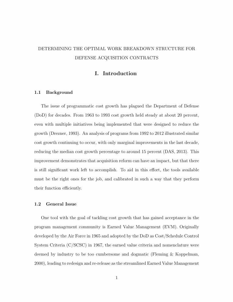
Program Work Breakdown Structure.

The Program Work Breakdown Structure (PWBS) represents the entire program.

For example an entire aircraft would require a Program WBS. This is used by the

government program manager for strategic decision making and long term visibility.

While the Program WBS is a living document early in the pre-program phases, after

iterative refinements it should become relatively static, representing a bottoms up

understanding of the program with buy-in from all stakeholders (Richardson, 2010).

An example based on MIL-STD-881C of the first three levels of a PWBS is illustrated

in Figure 1.

9

Aircraft SystemLEVEL 1

LEVEL 2

LEVEL 3

Air Vehicle TrainingProgram

ManagementSystems Engineering

Peculiar Support

Equipment

Airframe Avionics Propulsion Vehicle Subsystems

Figure 1. Example Program WBS

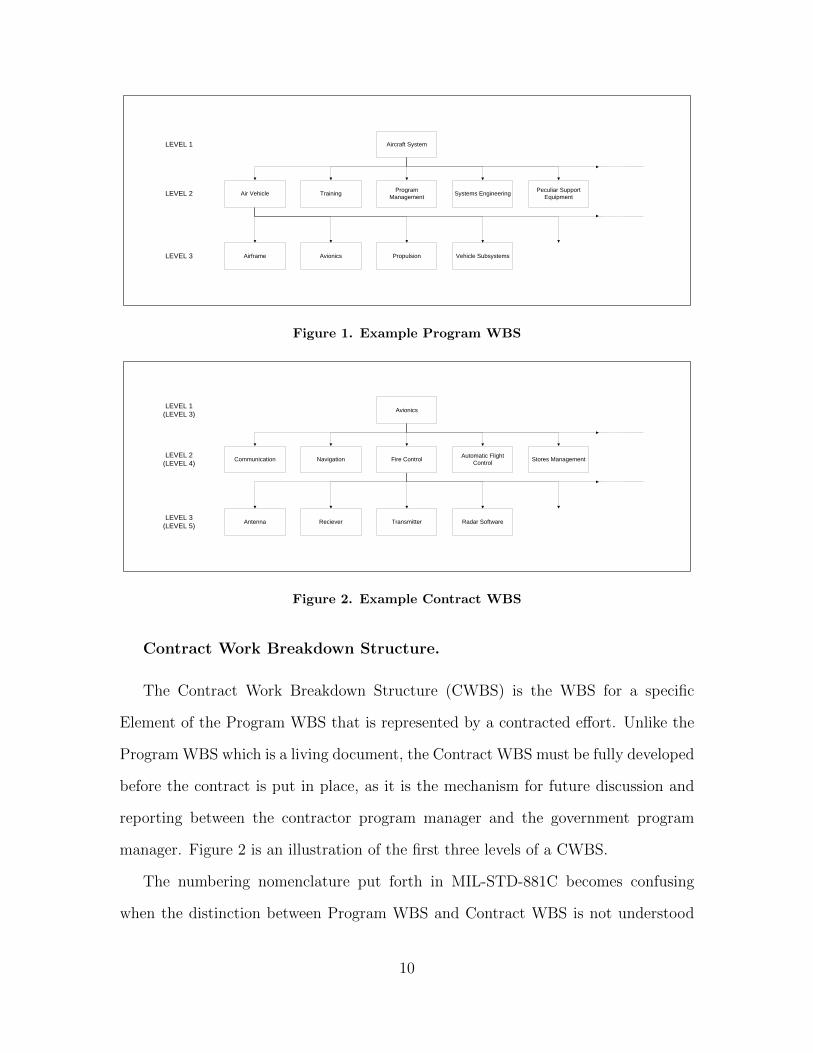
AvionicsLEVEL 1

(LEVEL 3)

LEVEL 2

(LEVEL 4)

LEVEL 3

(LEVEL 5)

Communication Navigation Fire ControlAutomatic Flight

ControlStores Management

Antenna Reciever Transmitter Radar Software

Figure 2. Example Contract WBS

Contract Work Breakdown Structure.

The Contract Work Breakdown Structure (CWBS) is the WBS for a specific

Element of the Program WBS that is represented by a contracted effort. Unlike the

Program WBS which is a living document, the Contract WBS must be fully developed

before the contract is put in place, as it is the mechanism for future discussion and

reporting between the contractor program manager and the government program

manager. Figure 2 is an illustration of the first three levels of a CWBS.

The numbering nomenclature put forth in MIL-STD-881C becomes confusing

when the distinction between Program WBS and Contract WBS is not understood

10

or taken into account. As Figure 2 demonstrates, the Level 1 of a Contract WBS

represents a Level 3 Element of the Program WBS. Further distinction must be made

between the CWBS that the contractor uses for internal program management, and

the CWBS that is reported to the government to satisfy the MIL-STD-881C require-

ments.

Contractor Contract Work Breakdown Structure.

The Contractor Contract WBS (C-CWBS) is designed by the contractor to inter-

nally manage the program. The expectation set forth in MIL-STD-881C (2.5.3) is

that the contractor will extend the CWBS, “...to the appropriate lower level that sat-

isfies critical visibility requirements and does not overburden the management control

system.” While the contractor might not follow the industry heuristic of extending

the C-CWBS to work packages containing approximately 80 hours of effort due to the

large size of the programs, industry best practice still calls for the final WBS to con-

tain a set of appropriately small work packages as the lowest elements (Richardson,

2010).

Government Contract Work Breakdown Structure.

A summary of the data from the C-CWBS is reported to the Government Program

Manager for the Government’s control effort in the form of the Government Contract

WBS (G-CWBS). MIL-STD-881C (1.5.3.C) notes that, “A WBS can be expressed

to any level of detail. While the top three levels are the minimum required for

reporting purposes on any program or contract, effective management of complex

programs requires WBS definition at considerably lower levels.” Justifiable reasons

for requiring increased granularity include elements that are high-cost, high-risk, or of

a specific technical nature. “In this case, managers should distinguish between WBS

11

definition and WBS reporting. The WBS should be defined at the level necessary to

identify work progress and enable effective management, regardless of the WBS level

reported to program oversight” (MIL-STD-881C).In order to differentiate between

the lowest element of the C-CWBS - a work package, the term “Leaf Element” will

be used when describing the most granular elements of the G-CWBS.

2.3 Earned Value Management

The Undersecretary of Defense for Acquisition Technology & Logistics’ Perfor-

mance Assessments and Root Cause Analyses office defines EVM as a, “... program

management tool to provide joint situational awareness of program status and to as-

sess the cost, schedule, and technical performance of programs for proactive course

correction.” Furthermore, EVM is required on Cost/Incentive contracts per DODI

5000.02 depending on total program cost, and is rarely used on fixed price contracts.

Characteristics of EVM include requiring a fully defined baseline integrating tech-

nical scope and authorized funding and personnel, set within an established schedule,

as well as mechanisms providing program managers early warning about program-

matic issues enabling course corrections in a timely manner (Fleming & Koppelman,

2000). The Contract Performance Report (CPR) is the primary means of communi-

cating EVM data from the contractor to the government, providing cost and schedule

performance data that can be used to identify programmatic issues and forecast fu-

ture performance (MIL-STD-881C). EVM can be applied to a specific period, or as a

cumulative measure. As the period calculations vary significantly and are individually

not useful for forecasting, focus will be given primarily to the cumulative measures

explained next.

12

Budgeted Cost of Work Scheduled. The budgeted cost of work scheduled

(BCWS) or Planned Value (PV) represents the dollars that are planned to be spent

on work efforts for a given time period. This figure can also represent the cumulative

budgeted cost of work scheduled from contract initiation through the current period.

BCWS = Budgeted Cost of Work Scheduled (1)

Budgeted Cost of Work Performed. The budgeted cost of work per-

formed (BCWP) or Earned Value (EV) represents the dollars that were planned to

be spent on work efforts regardless of the time period that the work was actually

accomplished. This figure can also represent the cumulative budgeted cost of work

performed from contract initiation through the current period.

BCWP = Budgeted Cost of Work Performed (2)

Actual Cost of Work Performed. The actual cost of work performed

(ACWP) or Actual Cost (AC) represents the dollars that were actually spent on

work efforts at the time they were actually accomplished, regardless of the original

time period or planned cost. This figure can also represent the cumulative actual cost

of work performed from contract initiation through the current period.

ACWP = Actual Cost of Work Performed (3)

13

Schedule Variance. In order to determine if a program is ahead or behind

schedule, Schedule Variance (SC) can be calculated by subtracting the budgeted cost

of work that should have been done by the period under review from the budgeted

cost of work that has actually been completed by the period under review.

SV = BCWP −BCWS (4)

Schedule Variance(t). Schedule Variance derived from (4) will converge

to 1.0 by definition, rendering it useless for analysis after approximately the 60%

completion point (Richardson, 2010). An alternative calculation has been proposed

and refined as a separate branch of EVM theory called Earned Schedule (ES) which

makes use of elapsed time t instead of elapsed dollars. The calculation of schedule

variance by ES in noted as SV (t), and is presented here for completeness, however the

earned schedule formulations will remain outside the scope of the current investigation

which focuses on the estimates that can be made in the first half of the program’s

schedule, and would thus not benefit significantly from implementing ES.

SV (t) = Earned Schedule− Actual T ime (5)

Cost Variance. In order to determine if we are over or under budget, Cost

Variance (CV) can be calculated by subtracting the actual cost of work that has been

accomplished by the period under review from the budget cost of work that has been

accomplished by the period under review.

CV = BCWP − ACWP (6)

14

Cost Performance Index. Allowing an understanding of cost efficiency

is the Cost Performance Index (CPI). This is calculated by taking the ratio of the

budgeted amount to the actual cost for work performed. If the actual cost is greater

than the budgeted cost, the performance index is less than 1.0 representing inefficient

use of funds. This index can be calculated using either period or cumulative measures.

CPI =BCWP

ACWP(7)

Schedule Performance Index. Similar to the CPI, the Schedule Perfor-

mance Index (SPI) provides a way of reporting schedule efficiency. This index can

also be calculated using either period or cumulative measures.

SPI =BCWP

BCWS(8)

Schedule Performance Index(t). Similar to SV (t), SPI can be calculated

using the Earned Schedule method.

SPI(t) =Earned Schedule

Actual T ime(9)

Estimate At Completion - CPI Method. In order to forecast the total

cost of the completed effort, the Estimate At Completion (EAC) can be calculated

in a few different ways. A primary method involves taking cost efficiency in the form

of the cumulative CPI into account.

EACCPI = ACWPCUM +BAC −BCWPCUM

CPICUM(10)

Estimate At Completion - Composite Method. A more complex method

of calculating EAC is the composite method where both the cost and schedule effi-

15

ciencies are taken into account. This is generally seen as the worst case scenario EAC

estimate and is often used as an upper bound for planning purposes. This formula

uses either the standard SPI calculation as an input, or the ES SPI(t), as well as

potentially imposing weights on the cumulative CPI and SPI.

EACComposite = ACWPCUM +BAC −BCWPCUMCPICUM ∗ SPICUM

(11)

With an understanding of Work Breakdown Structures, Earned Value Manage-

ment concepts and mechanics, and the policy foundation requiring cost and schedule

reporting, a review of previous research surrounding optimal WBS structuring will

be provided.

2.4 Previous Research

The policy that requires cost and schedule reporting leaves ample space for pro-

gram managers to customize their management approach, however the guidance on

how to use the flexibility on WBS formulation is sparse. Attempts to answer the

question of the most useful structure and level of reporting for program manage-

ment control have been both qualitative and quantitative. A short summary of these

previous efforts is reported next.

Qualitative Research.

Thomas (1999) and Bushey (2007) investigated the implementation of reporting

policy and presented conceptual frameworks for more useful implementation. Thomas

found that the policy in place had detrimental affects on improvement initiatives, and

Bushey proposed significantly increasing the contractor reporting requirements.

Thomas provides an in-depth review of the literature surrounding the creation and

implementation of the MIL-HBK-881, and attempts to determine if the policies it con-

16

tains actually impede acquisition reform initiatives and a PMs ability to manage. He

bases his findings that the policy does in fact hinder acquisition reform initiatives and

program management based on personal experience and interviews with government

and contractor personnel. He posits that a WBS prepared in accordance with (IAW)

MIL-HBK-881 will not provide sufficient insight into many of the elements.

The concept that limiting reporting at too broad a level will inhibit a PM’s ability

to manage is not controversial, but this scenario is only likely if the PM does the

minimum required by the MIL-HBK-881. That policy directs the PM to ensure that

their WBS is broken out to sufficient detail to allow visibility. What seems to be

lacking in the PM community is a method for determining when sufficient detail has

been achieved, or when further break-out is required.

Bushey describes the appropriate level of breakout in qualitative terms, noting

that an effective cost reporting structure requires flexibility to enable various forms

of analysis. EVM practiced at the program level only does not provide this flexibility,

because there is no ability to determine root-causes of issues with such a high level

data point. He goes on to propose a WBS structure down to the Work Package level,

as this will allow identification of root causes in cost and schedule discrepancies,

and facilitate discussions with the Control Account Managers (CAMs) who are in

a position to provide information and alternative action recommendations to the

government PM.

This recommendation is correct within the vacuum of a desire for visibility. It

is not, however, practical, and does not consider the flexibility by the contractor to

modify individual work packages without going through the bureaucratic maneuvers

necessary to modify the Government Contract WBS. The implementation of reporting

at the Work Package level would increase the reporting burden on the contractor, as

17

well as contractually require approval for every minor modification, both of which

would increase the cost to the government.

Quantitative Research.

Quantitative efforts surrounding report structuring and the value of lower level

reporting have focused on the predictive ability of lower level data elements compared

to the same data element reported at a higher level within the same program.

Rosado (2011) attempted to determine if overall program EVM characteristics

were consistent throughout the lower levels of the WBS. With a data set of 34 pro-

grams, he was able to demonstrate a correlation between the Development Test &

Evaluation element at level 3 and the program EAC. While helpful in forecasting

potential EAC growth, this result provides limited insight into the actual value of ac-

quiring lower level WBS data, however Rosado concludes that there is, “... potential

for improved prediction models using low level WBS EV data.”

Johnson (2014) built on Rosado’s research and attempted to determine if elemental

EVM data at Level 5 could provide earlier detection of cost growth than Level 3

EVM data. With a data set of 40 ACAT I programs, he concluded that elemental

information at Level 5 provided no useful increase in predictive capability compared

to Level 3 data.

Keaton (2015) took a narrow focus on 9 space acquisition contracts in an attempt

to determine if using lower level EVM data could better predict final cost estimates.

An issue that arose was the presence of great variability in the lower level WBS

elements making comparisons across contracts difficult. Due to the variability across

the contracts, the small sample size, and the method of comparing specific elements,

Keaton concluded that, “ ...lower level WBS data does not improve space program

EAC accuracy.”

18

2.5 Summary

In this chapter, a review of the reporting requirements outlined in DoDI 5000.02

and MIL-STD-881C has been presented requiring the use of Earned Value Manage-

ment on specific government acquisition contracts. The Work Breakdown Structure,

which details the reportable elements for EVM, was presented in three forms, the

Program WBS, the Contractor-Contract WBS, and the Government-Contract WBS.

A primer on Earned Value Management metrics was presented detailing the formulas

to be used, as well as explaining their meaning. Finally a review of previous research

showed that qualitative studies have found that minimal adherence to the reporting

guidelines produces data of minimal usefulness, and requiring G-CWBS broken out

to the Work Package level has been proposed as a response. Quantitative analysis

has resulted in an argument for using Level 3 data instead of relying on only pro-

gram Level 1 data for management decisions, but has not yet demonstrated increased

predictive ability from using lower than Level 3.

19

Bibliography



2. Department of Defense (2011). Department of Defense Standard Practice Work

Breakdown Structures for Defense Materiel Items (MIL-STD-881C). Washington,

DC: U.S. Government Printing Office.

3. Department of Defense, (2013). Performance of the Defense Acquisition System.

Washington, D.C.: U.S. Government Printing Office.


schedules (No. RAND/R-3937-ACQ). RAND Corp Santa Monica CA.

5. Eisner, H. (2008). Essentials of project and systems engineering management. John

Wiley & Sons.

6. Fleming, Q. (1992). Cost/schedule control systems criteria: The management

guide to C/SCSC. Chicago, Ill.: Probus Pub.






ing and Management.




20

10. Project Management Institute (PMI). (2000). A Guide to the Project Manage-

ment Body of Knowledge (PMBOKr), D-5. Project Management Institute, Penn-

sylvania.



12. Rosado, W. R. (2011). Comparison of Development Test and Evaluation and

Overall Program Estimate at Completion (No. AFIT/GCA/ENC/11-02). Air

Force Institute of Technology Wright-Patterson AFB OH Graduate School of En-

gineering and Management.



14. Under Secretary of Defense for Acquisition, Technology, and Logistics (2015).

Operation of the Defense Acquisition System (DODI 5000.02). Washington, DC:

U.S. Government Printing Office.

21

III. Alternative Formulation of a Pessimistic Estimate atCompletion

Abstract

Lack of visibility into contractors’ handling of specific work packages is an issue

that degrades government program managers’ ability to identify and remedy program-

matic issues. While Earned Value Management(EVM) provides a cost and schedule

control framework, current work breakdown structures are rarely granular enough

to provide actionable insight before issues become unmissable and generally uncor-

rectable. This paper presents an alternative formulation of the EVM metric Estimate

At Completion(EAC), that provides a pessimistic estimate for each leaf element based

on the cost and schedule performance index variance and dollar weight of all leaf ele-

ments. Creating this formulation required a new method to calculate index variance

that maintained the values in unit space. The new formulation, EACG−, provided a

true upper bound in over 85% of programs studied, and enables EVM practitioners

the ability to identify elements that are not sufficiently granular which would require

additional program management attention.

3.1 Introduction

A problem in program management is a lack of visibility to contractor movements

of work package efforts. Visibility is limited to the agreed upon form of the Con-

tract Work Breakdown Structure (CWBS) used to report Earned Value Management

(EVM) data. While EVM has been the cost and schedule control tool of choice for the

past two decades, there is still room for improvement in practice and understanding.

One such area of improvement is the method of calculating a pessimistic Estimate

At Completion (EAC). A review of the data presented in Section 1.2 shows that the

22

current method of calculation, EACComp, does not estimate an appropriate upper

bound in over 85% of programs studied1. Adding to this issue is the gross disparity

in weight between reported elements, with a range of weights between 100% of total

program costs to less than 0.001% of total program costs2. This wide range skews

the intuitive interpretation of the metrics calculated for those elements. A better

tool that accounts for element weight and provides a more consistent upper bound is

desirable to highlight those areas of a contract that will need special program man-

agement attention. A method of calculating a pessimistic EAC by placing confidence

limits may provide such a tool. The objective of this paper is to present an alternative

formulation of EACComp, based on element weight, which provides a more consistent

upper bound to final program cost than the currently employed pessimistic method.

Background.

In order to ensure consistency of terms, Table 1 is provided. All terms should be

familiar to EVM practitioners, with the exception of the term Leaf, which has been

proposed in order to contrast work package in terms of government visibility. The

issue of visibility is illustrated simply in Figure 1. This figure shows the invisible

work packages that make up the lowest level of data reported by the contractor to

the government. As this reported element is at the end of the WBS branch reported

to the government, the element will be referred to as a leaf. This is in contrast to the

work packages, which are in fact the lowest level of management breakout, and which

are visible to the contractor. The top set of work packages in the figure represent

how the work is planned, and its level of difficulty. The second set of work packages

illustrates that the contractor was able to shift the work packages within the leaf

element, based on difficulty. Finally, the lowest rows of the figure show that based

1Calculated Comparing the Program EAC at 10% complete against the Program EAC at 60%complete

2Further breakout with distribution by branch is illustrated in Figures 2,3,4, and 5

23

on the movement of work packages within the leaf element, the Cost Performance

Index (CPI) and Schedule Performance Index (SPI) metrics appear to be acceptable

through period 4. After this point the SPI metric will trend toward unity, and the

CPI metric has a significant drop off. Only after this point would the EVM metric

alert the Program Manager (PM) to potential issues caused by the difficult work

packages. While Figure 1 represents a very small effort, the issue it illustrates, that a

lack of visibility within the leaf element reduces a PM’s ability to effectively manage

their program, needs to be addressed.

Figure 3. Notional Leaf

Data.

The data used for analysis was retrieved from the Office of the Secretary of De-

fense’s Cost Assessment Data Enterprise (OSD CADE) system. Of the 276 contract

files available in the database, 108 had EVM data broken out into WBS elements,

of which 74 contracts had data representing over 60% contract completion. The pro-

gram contracts used for analysis are listed in Tables 2, 3, 4, and 5, and demographic

information is illustrated in Tables 2, 3, 4, and 5. The decision to include programs

with over 60% contract completion was based on a desire to include as many pro-

grams as possible, and is supported by the analysis illustrated in Figures 6 and 7,

24

Table 1. Review of Terms and Equations

Term Description

BCWS Budgeted Cost of Work Scheduled (BCWS) or Planned Value (PV) represents the dollarsthat are planned to be spent on work efforts for a given time period.

BCWPBudgeted Cost of Work Performed (BCWP) or Earned Value (EV) represents the dollars thatwere planned to be spent on work efforts regardless of the time period that the work wasactually accomplished.

ACWPActual Cost of Work Performed (ACWP) or Actual Cost (AC) represents the dollars thatwere actually spent on work efforts at the time they were actually accomplished, regardlessof the original time period or planned cost.

C − CWBS

Contractor’s Contract Work Breakdown Structure (C-CWBS) - The contract work breakdownstructure that the contractor uses for internal management of a contracted effort, broken outto the work package level. No summarization occurs in the C-CWBS. All data is visible tothe contractor.

G − CWBSGovernment’s Contract Work Breakdown Structure (G-CWBS) - The contract work break-down structure that the government program manager receives control reports based on,summarized at a high level.

WorkPackage

Defined by the Program Management Institute as a deliverable or project work componentat the lowest level of each branch of the work breakdown structure (PMBOK, 2000). Asthe PMI’s definition is aimed toward industry practitioners, it is understood that the workbreakdown structure referred to in the definition is the C-CWBS.

LeafTerm used to differentiate the terminal information node of a G-CWBS, compared to the workpackage of the C-CWBS. The leaf element represents an element that no longer branches intofurther elements.

Term Equation Description

CPI BCWPACWP

Cost Performance Index (CPI) allows an understanding ofcost efficiency. This is calculated by taking the ratio of thebudgeted amount to the actual cost for work performed.If the actual cost is greater than the budgeted cost, theperformance index is less than 1.0 representing inefficientuse of funds.

SPI BCWPBCWS

Schedule Performance Index (SPI), similar to the CPI, theSchedule Performance Index (SPI) provides a way of re-porting schedule efficiency.

EACComp ACWPCUM +BAC−BCWPCUMCPICUM∗SPICUM

Estimate at Complete (Composite Method) is a more com-plex method of calculating EAC where both the cost andschedule efficiencies are taken into account. This is gen-erally seen as the worst case scenario EAC estimate andis often used as an upper bound for planning purposes.This formula can uses either the standard SPI calculationas an input, or the ES SPI(t), as well as imposing weightson the CPI and SPI.

which shows that the budget at complete (BAC) is significantly less variable after

the 60% completion point, with a mean change less than 7%. Focus was placed on

BAC stability as this is the metric that was the baseline for the comparative tests

between the current pessimistic EAC and the alternative EAC presented. Also of

note, specific programmatic anomalies are visible in Figure 6, but this data was left

in the analysis as no justification for its removal was found.

Previous Methods.

Statistical methods have been applied to Earned Value Management generally

(Lipke & Vaughn, 2000; Lipke, 2002; Anbari, 2003; Lipke, 2006; Wang, Jiang, Gou,

25

Figure 4. Army Demographics

Che, & Zhang, 2006; Leu & Lin, 2008), and to forecasting Schedule Performance Index

specifically (Lipke, Zwikael,Henderson, & Anbari, 2009; Colin & Vanhoucke, 2014).

A common method presented in these studies was to transform the index data into

natural log space in order to estimate the parameters required to calculate confidence

limits. This transformation is very appealing due to its ability to normalize the index

data which is often very skewed, its ease of implementation, and certain properties

of the log-normal distribution which proved useful for various assumptions that were

made in the previous research. In particular the confidence limit standard deviation

requires a mean value for calculation, and the natural log of the cumulative index

value is reported as being a good estimator (Lipke, 2009).

26

Figure 5. Navy Demographics

While the natural log transformation is appealing, its use proved problematic

in the current study for three reasons. Two issues stem from using the cumulative

index value as an estimator of the index mean. Computationally, this would require

sufficient time to have passed to enable enough periods to accrue that would yield

a suitable cumulative index value. This is undesirable in that information is desired

earlier, while the validity of that information increases as time passes. An inference

made too early is likely invalid, while an inference made on valid data is likely too late

to be of use. The second issue is purpose. The fact that the cumulative index value is

a good estimate of the mean is the very problem that the current study is aiming to

address, in that the cumulative index represents an average. Averages hide significant

27

Figure 6. Air Force Demographics

values, and it is specifically those values that need to be highlighted for program

management oversight. The final issue that precluded the use of the log-normal

transformation is its inability to appropriately treat weighting. As a central concept

in the problem is that elements have a range of weights, this must be accounted

for in the confidence limit calculations, which proved problematic using log-normal

transformed data.

28

Figure 7. Joint Demographics

Proposed Method.

It will be useful to first describe the phenomena under investigation. The indexes

focused on are represented by Equations 12 and 13.

CPI =BCWP

ACWP(12)

SPI =BCWP

BCWS(13)

both of which can be generalized to

29

Figure 8. Delta From Final BAC

Index =Constant

V ariable(14)

or:

Y =K

X(15)

which transforms into:

Y = K−X (16)

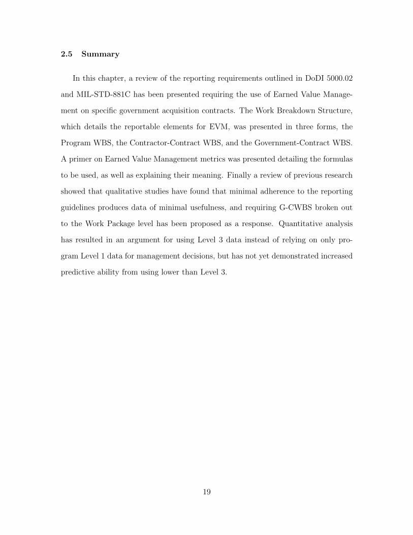
The graph of Equation 16 when K = 1 is plotted, along with the identity line

y = x, in Figure 8. The index essentially tells the analysts the magnitude in dollars

away from the expected value of the program for either schedule or cost. For example,

if the expected cost is $1000 and the actual cost is $200, then the CPI = 1000200

= 5.

This tells the analyst that the actual cost was 5 times less than expected. The same

dollar value difference as a cost overage, represented by CPI = 10001800

= 0.55, represents

the magnitude away from expected along the curve below the identity line; therefore

in order to calculate the magnitude the reciprocal must be taken: 10.55

= 1.8. The

30

Figure 9. Difference of Means Test

analyst therefore knows that at CPI = 0.55 the element is 1.8 times more than

expected. A general form of this principle used to find the magnitude away from

expected value in the index is given in Equation 17. Note that the reciprocal form is

negative due to the fact that it is undesirable and below the identity line.

Magnitude =

Index ≥ K : Index

Index < K : − KIndex

(17)

This transformation normalizes the index data around the constant K, just as

the log-normal transform espoused by previous studies, however with the benefit of

staying in unit space as opposed to going into log space. This is essential as the

weight of each element is described as a percentage in unit space.

Now with an understanding of the environment the indexes reside in, factors con-

tributing to the lack of visibility can be addressed. One of the issues that plague the

current Government Contract WBS (G-CWBS) Leaf elements’ ability to accurately

reflect program cost and schedule efficiencies arise from the variance in sizes of the

leaf elements. A leaf element that represents 10% of the contract with an unfavorable

31

Table 2. Army Programs

Program Branch Months Phase ContractBLACK HAWK UPG Army 56 RDTE Cost Plus

EXCALIBER Army 17 PROD Cost PlusFBCB2 Army 68 RDTE Cost Plus

GCSS ARMY Army 83 RDTE Cost PlusGCV Army 25 NA Fixed Price IncentiveIAMD Army 61 RDTE Cost PlusJAGM Army 26 RDTE Fixed Price IncentiveJLTV Army 22 RDTE OtherJTN Army 55 NA Cost Plus

JTRS GMR Army 74 NA OtherLMP2 Army 13 NA Cost PlusMH60R Army 51 RDTE Cost PlusMH60S Army 48 NA Cost Plus

PAC3MSE Army 31 NA Cost PlusPatriotMeadsCap Army 59 NA Other

STRYKER Army 53 RDTE Cost PlusTMC Army 42 NA Cost PlusWIN2 Army 35 RDTE Cost PlusWIN3 Army 39 RDTE Cost Plus

CPI = .5 should have more impact than a leaf element representing 0.5% of the

contract with a favorable CPI = 2. Therefore, any tool devised must handle this dis-

crepancy in sizing. The method chosen for the EACG formulation is to calculate the

weighted standard deviation (Formula 18) where wi is the weight (calculated as BACi

BAC)

of the Leaf xi, and xi represents the magnitude of the efficiency metric being studied.

Using the weighted variance calculation will reduce the impact of any extreme data

values that do not represent a large portion of the effort, while giving more power to

the index data points that represent the majority of the program effort.

s =

√√√√√√√√

n∑i=1

wix2i ∗

n∑i=1

wi −(

n∑i=1

wixi

)2

(n∑i=1

wi

)2

−n∑i=1

w2i

(18)

The leaf elements of the G-CWBS represent the whole contracted effort, and

yet do not represent each individual work package. From this perspective, the leafs

32

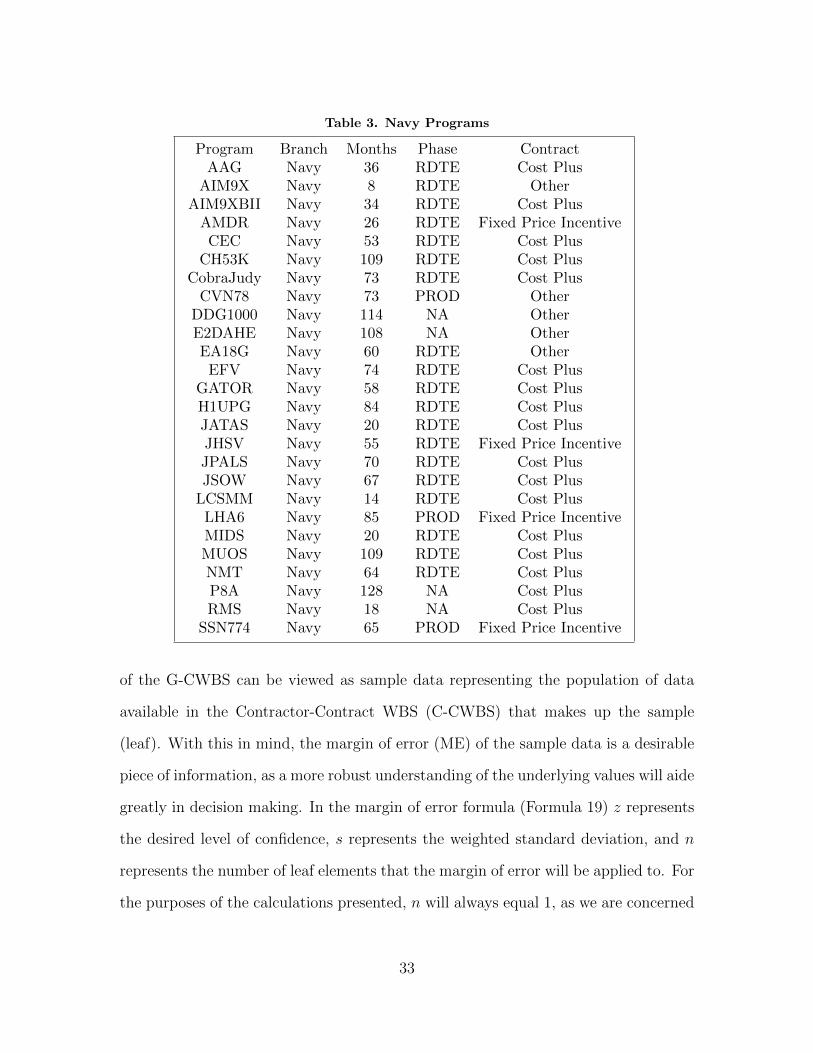
Table 3. Navy Programs

Program Branch Months Phase ContractAAG Navy 36 RDTE Cost Plus

AIM9X Navy 8 RDTE OtherAIM9XBII Navy 34 RDTE Cost PlusAMDR Navy 26 RDTE Fixed Price IncentiveCEC Navy 53 RDTE Cost Plus

CH53K Navy 109 RDTE Cost PlusCobraJudy Navy 73 RDTE Cost PlusCVN78 Navy 73 PROD Other

DDG1000 Navy 114 NA OtherE2DAHE Navy 108 NA OtherEA18G Navy 60 RDTE OtherEFV Navy 74 RDTE Cost Plus

GATOR Navy 58 RDTE Cost PlusH1UPG Navy 84 RDTE Cost PlusJATAS Navy 20 RDTE Cost PlusJHSV Navy 55 RDTE Fixed Price IncentiveJPALS Navy 70 RDTE Cost PlusJSOW Navy 67 RDTE Cost PlusLCSMM Navy 14 RDTE Cost PlusLHA6 Navy 85 PROD Fixed Price IncentiveMIDS Navy 20 RDTE Cost PlusMUOS Navy 109 RDTE Cost PlusNMT Navy 64 RDTE Cost PlusP8A Navy 128 NA Cost PlusRMS Navy 18 NA Cost Plus

SSN774 Navy 65 PROD Fixed Price Incentive

of the G-CWBS can be viewed as sample data representing the population of data

available in the Contractor-Contract WBS (C-CWBS) that makes up the sample

(leaf). With this in mind, the margin of error (ME) of the sample data is a desirable

piece of information, as a more robust understanding of the underlying values will aide

greatly in decision making. In the margin of error formula (Formula 19) z represents

the desired level of confidence, s represents the weighted standard deviation, and n

represents the number of leaf elements that the margin of error will be applied to. For

the purposes of the calculations presented, n will always equal 1, as we are concerned

33

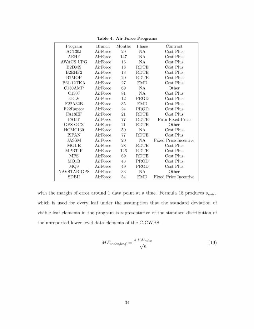
Table 4. Air Force Programs

Program Branch Months Phase ContractAC130J AirForce 29 NA Cost PlusAEHF AirForce 147 NA Cost Plus

AWACS UPG AirForce 13 NA Cost PlusB2DMS AirForce 18 RDTE Cost PlusB2EHF2 AirForce 13 RDTE Cost PlusB2MOP AirForce 20 RDTE Cost Plus

B61-12TKA AirForce 27 EMD Cost PlusC130AMP AirForce 69 NA OtherC130J AirForce 81 NA Cost PlusEELV AirForce 12 PROD Cost Plus

F22A32B AirForce 35 EMD Cost PlusF22Raptor AirForce 24 PROD Cost PlusFA18EF AirForce 21 RDTE Cost PlusFABT AirForce 77 RDTE Firm Fixed Price

GPS OCX AirForce 21 RDTE OtherHCMC130 AirForce 50 NA Cost PlusISPAN AirForce 77 RDTE Cost PlusJASSM AirForce 20 NA Fixed Price IncentiveMGUE AirForce 28 RDTE Cost PlusMPRTIP AirForce 126 RDTE Cost PlusMPS AirForce 69 RDTE Cost PlusMQ1B AirForce 43 PROD Cost PlusMQ9 AirForce 49 PROD Cost Plus

NAVSTAR GPS AirForce 33 NA OtherSDBII AirForce 54 EMD Fixed Price Incentive

with the margin of error around 1 data point at a time. Formula 18 produces sindex

which is used for every leaf under the assumption that the standard deviation of

visible leaf elements in the program is representative of the standard distribution of

the unreported lower level data elements of the C-CWBS.

MEindex,leaf =z ∗ sindex√

n(19)

34

Table 5. Joint Programs

Program Branch Months Phase ContractAHLTA Joint 18 PROD Cost PlusBCS F3 Joint 74 RDTE Cost Plus

ChemDemil Joint 78 RDTE OtherDTS Joint 18 PROD Cost Plus

3.2 Methods

Margin of Error Application.

The application of the margin of error occurs differently depending on the position

of the initial index point (X) when compared to the identity line (K), and the size of

the margin of error and whether or not its application requires crossing the identity

line. The equation for applying the margin of error given each possible scenario is

given by Equation 20, and the various implementations are illustrated and described

forthright.

X +

X < K

ME ≤ |K − KX| : K

KX−ME

ME > |K − KX| : K +ME + (K − K

X)

X ≥ K

ME < X −K : X +ME

ME ≥ X −K : X +ME

X −

X < K

ME ≤ |K − KX| : K

KX

+ME

ME > |K − KX| : K

KX

+ME

X ≥ K

ME < X −K : X −ME

ME ≥ X −K : KK+(ME−(X−K))

(20)

35

Figure 10. Reciprocal Function

X ≥ K;ME ≤ X −K.

For cases where the Index point is greater than or equal to K, and the margin of

error is less than or equal to the difference of X and K, as illustrated in Figures 9 and

10, the following equations should be used for finding X ±ME, as the identity line

will not be crossed when finding the lower bound.

X +ME = X +ME (21)

X −ME = X −ME (22)

Equations 21 and 22 are very simple because they both occur above the identity line.

A simple addition and subtraction will suffice.

36

X ≥ K;ME > X −K.

For cases where the Index point is greater than or equal to K, and the margin

of error is greater than the difference of X and K, the following equations should be

used for finding X ±ME, as the identity line will be crossed when finding the lower

bound.

X +ME = X +ME (23)

X −ME =K

K + (ME − (X −K))(24)

Equation 23 is simply the addition of the margin of error to the index point. Equa-

tion 24 must take into account crossing K. X−K is the distance that must be traveled

along the Y axis to get to K. This distance is subtracted from ME as it has already

been traveled. The remaining distance must be added to K. This distance is then

placed under K in order to move along the X axis to the correct lower bound location.

X < K;ME ≤ |K − K/X|.

For cases where the Index point is less than K, and the margin of error is less

than or equal to the absolute value of the difference of K and the ratio of K and the

Index, as illustrated in Figures 11 and 12, the following equations should be used for

finding X ±ME.

The logic of this rule is that K − KX

represents the distance from K to X as can

be seen in Figure 11. KX

represents the nominal point value along the curve, and the

difference of K and KX

represents the distance along the curve that can be traveled

before crossing the identity line at K. Equations 27 and 28 are required when crossing

K. The absolute value is required when X < 0.5 as this would cause inconsistencies.

37

Figure 11. Lower CL Does Not Cross ID Line

X +ME =K

KX−ME

(25)

X −ME =K

KX

+ME(26)

Equations 25 and 26 handle the addition and subtraction of the margin of error to

X. Figure 11 shows the movement along the reciprocal curve from X. The restrictions

on the use of this equation ensure that the upper bound of the margin of error (denoted

by the connected black circles) does not cross the identity line. While the margin of

error has potentially significant lateral movement, there is little vertical movement

along the curve. This is why a margin of error totaling 6 (2 ∗ME) results in the

upper and lower bounds both remaining below 1. The logic of Equation 25 begins

38

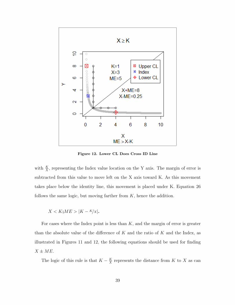
Figure 12. Lower CL Does Cross ID Line

with KX

, representing the Index value location on the Y axis. The margin of error is

subtracted from this value to move left on the X axis toward K. As this movement

takes place below the identity line, this movement is placed under K. Equation 26

follows the same logic, but moving farther from K, hence the addition.

X < K;ME > |K − K/X|.

For cases where the Index point is less than K, and the margin of error is greater

than the absolute value of the difference of K and the ratio of K and the Index, as

illustrated in Figures 11 and 12, the following equations should be used for finding

X ±ME.

The logic of this rule is that K − KX

represents the distance from K to X as can

39

be seen in Figure 12. KX

represents the nominal point value along the curve, and the

difference of K and KX

represents the distance along the curve that can be traveled

before crossing K. As the margin of error exceeds this amount, the identity line

will be crossed. The absolute value is required when X < 0.5 as this would cause

inconsistencies.

X +ME = K +ME + (K − K

X) (27)

X −ME =K

KX

+ME(28)

Equation 27 crosses the identity line. KX

represents the Index point’s location on

the X axis K − KX

represents the distance from the Index point to the identity line,

traveling on the X axis. This is a negative amount. The distance from K to the

margin of error number, plus this negative amount, results in the proper location

along the Y axis of the curve. Equation 28 is identical to Equation 26 as it performs

the same movement.

Calculate EACG.

In order to arrive at a true worst case estimate at completion for each leaf element,

the pessimistic limit (represented by the ‘−’ sign in the subscript) of both CPI and

SPI should be used to calculate the EACComp equation shown in Table 1. This new

formulation is presented in Formula 29.

EACComp.G,i,t,− = ACWPCUM,i,t +BACi,t −BCWPCUM,i,t

CPICUM.G,i,t,− ∗ SPICUM.G,i,t,−(29)

40

Figure 13. Upper CL Does Not Cross ID Line

Test Against Current Pessimistic EAC.

A comparative hypothesis test will determine if the Alternative EACComp.G,− pro-

vides a better worst case upper bound for EAC than the current worst case scenario

EACComp. The effectiveness of the metric will be graded using one tailed pairwise

Wilcoxon Rank Sum Test, determining if at times δ: 10%, 20%, 30%, 40%, and 50%

complete, the worst case EAC is actually more than the BAC reported at times φ:

60%, 70%, 80%, and 90% complete. The use of multiple comparison points enabled

the largest number of contracts to be analyzed and their results compared enabling

stronger inferences. The Wilcoxon Rank Sum Test was used as the assumptions re-

quired for a pairwise t-test could not be satisfied based on the characteristics of the

data. The pairwise test performed between the status quo pessimistic EAC and the

41

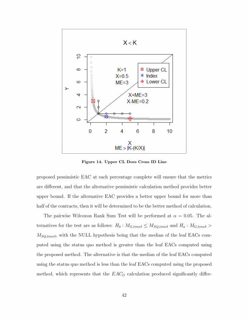
Figure 14. Upper CL Does Cross ID Line

proposed pessimistic EAC at each percentage complete will ensure that the metrics

are different, and that the alternative pessimistic calculation method provides better

upper bound. If the alternative EAC provides a better upper bound for more than

half of the contracts, then it will be determined to be the better method of calculation.

The pairwise Wilcoxon Rank Sum Test will be performed at α = 0.05. The al-

ternatives for the test are as follows: H0 : MG,timeδ ≤ MSQ,timeδ and Ha : MG,timeδ >

MSQ,timeδ, with the NULL hypothesis being that the median of the leaf EACs com-

puted using the status quo method is greater than the leaf EACs computed using

the proposed method. The alternative is that the median of the leaf EACs computed

using the status quo method is less than the leaf EACs computed using the proposed

method, which represents that the EACG calculation produced significantly differ-

42

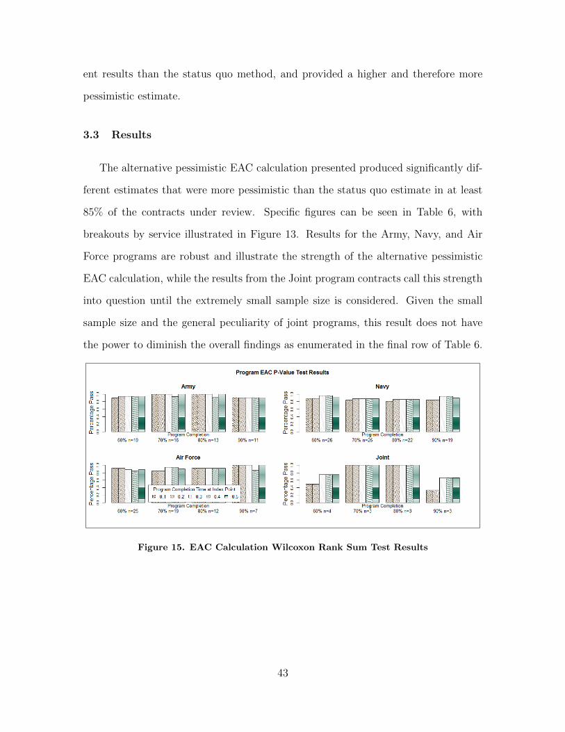
ent results than the status quo method, and provided a higher and therefore more

pessimistic estimate.

3.3 Results

The alternative pessimistic EAC calculation presented produced significantly dif-

ferent estimates that were more pessimistic than the status quo estimate in at least

85% of the contracts under review. Specific figures can be seen in Table 6, with

breakouts by service illustrated in Figure 13. Results for the Army, Navy, and Air

Force programs are robust and illustrate the strength of the alternative pessimistic

EAC calculation, while the results from the Joint program contracts call this strength

into question until the extremely small sample size is considered. Given the small

sample size and the general peculiarity of joint programs, this result does not have

the power to diminish the overall findings as enumerated in the final row of Table 6.

Figure 15. EAC Calculation Wilcoxon Rank Sum Test Results

43

Table 6. Summary of EAC Calculation Comparison Analysis

Test Point φ 0.6 0.7 0.8 0.9

Test Point δ 0.1 0.2 0.3 0.4 0.5 0.1 0.2 0.3 0.4 0.5 0.1 0.2 0.3 0.4 0.5 0.1 0.2 0.3 0.4 0.5

Result P-Val P-Val P-Val P-Val P-Val P-Val P-Val P-Val P-Val P-Val P-Val P-Val P-Val P-Val P-Val P-Val P-Val P-Val P-Val P-Val

Army 0.895 0.947 0.947 0.947 0.947 1 1 1 0.938 1 1 1 1 0.923 1 0.909 0.909 0.909 0.909 0.909

n=19 n=16 n=13 n=11


Navy 0.885 0.885 0.962 0.962 0.923 0.84 0.88 0.88 0.88 0.88 0.818 0.864 0.864 0.864 0.864 0.842 0.842 0.947 0.947 0.895

n=26 n=25 n=22 n=19


Air Force 0.92 0.92 0.88 0.84 0.88 0.842 0.842 0.947 0.947 0.895 0.917 0.917 0.917 0.917 0.917 1 1 1 0.857 1

n=25 n=19 n=12 n=7


Joint 0.5 0.5 0.75 0.75 0.75 1 1 1 1 1 1 1 1 1 1 0.333 0.333 0.667 0.667 0.667

n=4 n=3 n=3 n=3


Total 0.878 0.892 0.919 0.905 0.905 0.889 0.905 0.937 0.921 0.921 0.9 0.92 0.92 0.9 0.92 0.85 0.85 0.925 0.9 0.9

n=74 n=63 n=50 n=40

Test Point φ represents the point in time (% program complete) of the EAC that is taken as the true correct EAC

Test Point δ represents the point in time (% program complete) of the EAC that is compared to the EAC at Test Point φ

Result P-Val represents the % of programs whose Wilcoxon Rank Sum Test had a P-Value less than 0.05.

This result demonstrates that the two methods of calculation produced significantly different EAC sets.

3.4 Discussion and Conclusion

As the intent of producing an alternative EAC was to provide a better upper

bound pessimistic estimate, the proposed EACG satisfies that intent. It produces an

estimate that is more pessimistic than the current calculation of EACComp in over

85% of the contracts reviewed, demonstrating that it is indeed a better pessimistic es-

timate. With the validation of this estimate, it can now be used to address the issues

illustrated in Figure 1, by using the methods presented in this paper. For example,

a practitioner would be able to review current EVM information, calculate the pes-

simistic EAC for each element, and highlight those elements with a pessimistic EAC

greater than some subject matter expert derived risk tolerance level. These high-

lighted elements would represent elements that are most at risk within the program

based on the leaf index metrics and the dollar weight of those leaf elements. Elements

with alarmingly high pessimistic EACG likely do not provide enough granularity for

44

the program manager to simply rely on the reported EVM metrics. These are the

elements, like Figure 1, that may produce surprises late in the contract, and should

therefore be scrutinized through other channels in addition to EVM.

While this use has merit, it is reactive in nature. Using the proposed EACG,

formulation of a metric to grade the granularity of a contractor work breakdown

while still in the pre-award stage is an area of future research. This future metric

will endeavor to provide program managers actionable insight and greater ability to

formulate useful G-CWBSs, in a pro-active fashion.

This paper presented a background on Estimate At Completion calculation meth-

ods, discussion on the switch from calculating in natural log space to maintaining

calculations in unit space, as well as a proposed formula for calculating EAC bounds

based on the variability of the WBS leaf elements. The study demonstrated that the

upper bound predicted by the proposed formulation represents a better pessimistic

estimate than the current worst case EAC formulation by providing a true upper

bound in over 85% of the programs studied.

45

Bibliography

1. Anbari, F. (2003). Earned Value Project Management Method and Extensions.

Project Management Journal, 34(4),12-23.

2. Colin, J., and Vanhoucke, M. (2014). Setting Tolerance Limits for Statistical

Project Control Using Earned Value Management. Omega - International Jour-

nal of Management Science, 49, 107-122.

3. Leu, S., and Lin, Y. (2008). Project Performance Evaluation Based on Statistical

Process Control Techniques. Journal of Construction Engineering and Manage-

ment, 134(10), 813-819.

4. Lipke, W. (2002). A Study of the Normality of Earned Value Management Indica-

tors. The Measurable News, 4, 1,6,7,12-14,16.

5. Lipke, W. (2006). Statistical Methods Applied to EVM: The Next Frontier.

CrossTalk-The Journal of Defense Software Engineering, 19(6), 20-23.

6. Lipke, W., and Vaughn, J. (2000). Statistical Process Control Meets Earned Value.

CrossTalk-The Journal of Defense Software Engineering, 13(6), 16-20,28-29.

7. Lipke, W., Zwikael, O., Henderson, K., and Anbari, F. (2009). Prediction of Project

Outcome: The Application of Statistical Methods to Earned Value Management

and Earned Schedule Performance Indexes. International Journal of Project Man-

agement, 27(4), 400-407.

8. Project Management Institute (PMI). (2000). A Guide to the Project Management

Body of Knowledge (PMBOKr), D-5. Project Management Institute, Pennsylva-

nia.

46

9. Wang, Q., Jiang, N., Gou, L., Che, M., and Zhang, R. (2006). Practical Experi-

ences of Cost/Schedule Measure Through Earned Value Management and Statis-

tical Process Control. In Software Process Change, Vol. 3966 of Lecture Notes in

Computer Science, 348-354. Berlin, Germany: Springer.

47

IV. Generating Random DoD Program Data

4.1 Introduction

Department of Defense (DoD) acquisition programs are well known for their com-

plexity, and infamous for their tendency to experience budget growth. From the

current example of the Air Force’s F-35 program (Leonard & Wallace, 2014) to the

recent historical example of the Navy’s canceled A-12 program (GAO, 1992), DoD

acquisition history is littered with programs whose initial estimated cost ballooned.

The cause of this growth is a heavily discussed topic that will not be broached here.

Instead, the topic of this article is to address an issue that plagues those who ana-

lyze DoD budget growth: the issue of insufficient data (Rosado, 2011; Johnson, 2014;

Keaton, 2015).

This is not to say that the DoD is entirely lacking data. With the Weapon System

Acquisition Reform Act (WSARA) of 2009 and the mandates given to the Director of

Cost Assessment and Program Evaluation, there has been a large growth in available

data. The cost and schedule control Earned Value Management (EVM) data needed

for contract cost analysis have even been amassed into a useful and relatively (for

government analysts) accessible database maintained by the Office of the Secretary

of Defense called the Cost Analysis Data Enterprise (CADE). This access to data

is welcoming for practitioners, but appropriate replicates of different program types

which would enable robust analysis of macro trends and factors is still lacking.

The specific analysis this article focuses on, a brief overview of which is in Sec-

tion 2, is concerned with EVM data reported at varying levels of granularity, and

the effect that this granularity has on government program management’s ability

to control the program and make timely and informed management decisions. The

CADE system held 67 program contract data files that contained the work breakdown

48

structure (WBS) at different levels of granularity and reported in a format consistent

with governing regulations and guidelines (DoD, 2011; Fitzpatrick, Meyer, & Stubbs,

2016). These programs can be characterized by different demographic parameters

that can be filtered within the CADE database system. These demographics include

the responsible branch of service (4 levels), program phase (3 levels), contract vehicle

(3 levels), and system type (12 levels). When these simple demographic parame-

ters are considered, 432 combinations can be constructed. The 67 program files only

come from 44 of the demographic combinations, many being unique, with the most

numerous combinations having only 5 demographic replicates. This makes finding

analogous systems or pools of systems for parametric analysis unfeasible, reducing or

eliminating the rigor, benefit, and applicability of quantitative analysis.

Previous research has introduced the G-Score (Fitzpatrick, Meyer, & Stubbs,

2016), a metric that can be applied reactively to a program’s Work Breakdown

Structure, highlighting those leaf elements that are most at risk and require addi-

tional program management oversight beyond the normal cost and schedule control

tools of earned value management. These leaf elements are at risk because the WBS

in place is not granular enough to provide early warning that an underlying work

package within the leaf element is experiencing difficulties (Fleming & Koppelman,

2000; Fitzpatrick, White, Lucas, & Elshaw, 2016). This metric had to be applied

reactively because the WBS for the systems under review were already set, and no

further granularity was available for testing alternative structures. The G-Score has

the potential to be used prescriptively before the Work Breakdown Structure is so-

lidified at the time of contract award, being applied to compare the usefulness of

different WBS forms.

49

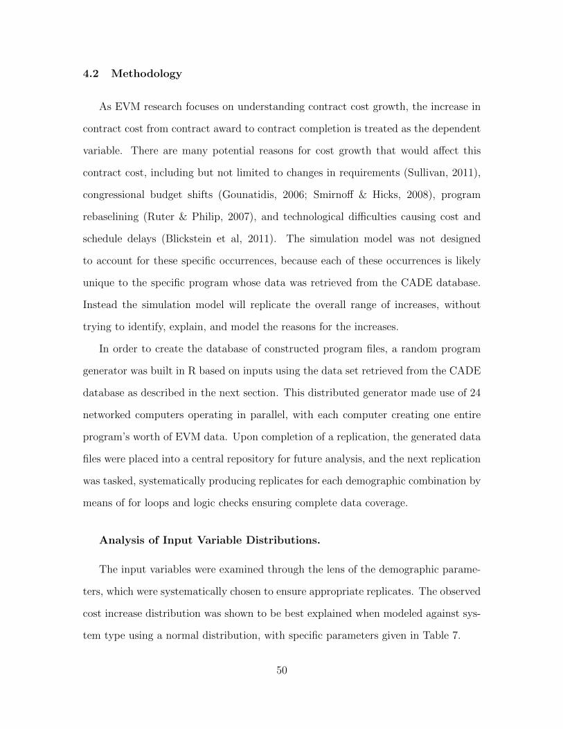
4.2 Methodology

As EVM research focuses on understanding contract cost growth, the increase in

contract cost from contract award to contract completion is treated as the dependent

variable. There are many potential reasons for cost growth that would affect this

contract cost, including but not limited to changes in requirements (Sullivan, 2011),

congressional budget shifts (Gounatidis, 2006; Smirnoff & Hicks, 2008), program

rebaselining (Ruter & Philip, 2007), and technological difficulties causing cost and

schedule delays (Blickstein et al, 2011). The simulation model was not designed

to account for these specific occurrences, because each of these occurrences is likely

unique to the specific program whose data was retrieved from the CADE database.

Instead the simulation model will replicate the overall range of increases, without

trying to identify, explain, and model the reasons for the increases.

In order to create the database of constructed program files, a random program

generator was built in R based on inputs using the data set retrieved from the CADE

database as described in the next section. This distributed generator made use of 24

networked computers operating in parallel, with each computer creating one entire

program’s worth of EVM data. Upon completion of a replication, the generated data

files were placed into a central repository for future analysis, and the next replication

was tasked, systematically producing replicates for each demographic combination by

means of for loops and logic checks ensuring complete data coverage.

Analysis of Input Variable Distributions.

The input variables were examined through the lens of the demographic parame-

ters, which were systematically chosen to ensure appropriate replicates. The observed

cost increase distribution was shown to be best explained when modeled against sys-

tem type using a normal distribution, with specific parameters given in Table 7.

50

Table 7. Cost Increase Distribution By System

System Type Mean Standard De-viation

Shapiro Wilkes P-Value

All 0.192537 0.20604 0.0138Aircraft System 0.183333 0.163649 0.7136Electronic System 0.251667 0.220701 0.9345Missile System 0.13 0.176352 0.0199Ordinance 0.188 0.334021 0.0045Sea System 0.12 0.111056 0.5027Space System 0.2975 0.251843 0.5Surface Vehicle 0.36667 0.086217 0.6788Unmanned Air System 0.125 0.049498 1Automated Information System .325 .250932 0.4346

The observed distribution of the number of months was fit using a Weibull distri-

bution, based on both the responsible branch and the phase of the program. Table

8 shows the parameters available, with the bold figures representing the variables

input to the model. The decision to use the scale parameter from one demographic

variable, and the shape parameter from another demographic variable, came about

during data exploration, and was supported by empirical observations and existing

policy. For example, the scale parameter dictated by phase reflected the mean number

of months for a program, which corresponds to fiscal law requirements limiting the

length of time for funds expenditure and full funding requirements (10 U.S.C. 2366b).

The shape parameter, influencing the skew of the distribution based on branch, cor-

responds with the type of items procured and the inherent lead time needed, such as

the difference between a new armored transport truck and a new aircraft carrier.

The initial program cost, or the estimated cost at completion (EAC) at time 0,

was shown to follow a log normal distribution based on branch as illustrated in Table

9. The Air Force did fail the goodness of fit test at α = 0.05, however the log normal

distribution had the most passing scores of the distributions investigated. For this

reason and to attempt to keep the model from growing in complexity, the log normal

was maintained as the best distribution.

51

Table 8. Month Distribution By Phase and Branch

By PhasePhase Scale Shape Cramer-von Mises W TestEMD 42.93187 3.73898 0.25RDTE 58.00806 1.836495 0.1364PROD 45.52715 1.686539 0.1881

By BranchBranch Scale Shape Cramer-von Mises W TestArmy 48.51867 2.72801 0.25Navy 66.21203 1.993546 0.1048Air Force 50.39073 1.439873 0.1048Joint 52.81163 1.663965 0.0521

Table 9. Initial Program Cost Distribution By Branch

Branch Scale µ Shape σ Kolmogorov’s DAll 19.17084 1.48063 0.01Army 19.05398 1.222855 0.1119Navy 19.69577 1.72445 0.0926Air Force 18.89883 1.76352 0.0494Joint 18.57293 1.172564 0.15

Simulation Variables.

With the program demographics systematically chosen, and the contract initial

cost, length, and cost growth characteristics determined based on those demograph-

ics, the remaining variables used in the stochastic model will be determined using

Monte Carlo methods. While Monte Carlo modeling has been used previously to

explore predictive capabilities of earned value management metrics (Colin & Van-

houcke, 2014), as well as monitoring and forecasting project performance (Barraza,

Back, & Mata, 2000; Barraza, Back, & Mata, 2004), it has not been found in the

literature to have been used to create entire program contracts.

The input parameters of the simulation variables have been modeled with many

different distribution shapes. Where possible, input values are empirically derived

from the observed programs in the CADE database. Where this is not possible,

parameters were taken from previous studies found throughout the literature to create

52

distributions. When the literature was barren, the remaining parameters were created

using a Bayesian approach with initial values coming from the authors’ experience and

discussions with defense acquisition personnel. These parameters were then iteratively

tuned to arrive at the posterior distributions (Kennedy & O’Hagan, 2001). The

specific distributions and sources are presented in Table 10. Those parameters that

were based on the Bayesian estimator approach lended themselves more toward the

triangular distribution, as the data was lacking to fit a more nuanced form.

Table 10. Variable Distributions

Triangular DistributionsVariable Min Max Mode JustificationAvg Fully Burdened Labor Rate (AvgFBLR)

130 200 150 Bayesian Calibration

Software Growth Multiplier 0.9 1.9 1.3 Literature (Holchin, 2003)Easy Work Package Shift 0.1 1.0 0.6 Bayesian CalibrationHard Work Package Shift 1 12 4 Bayesian CalibrationWork Package Time Delay 0 2.5 0.25 Bayesian CalibrationTechnology Readiness Level Min Max Med Bayesian Calibration

Normal DistributionsVariable Mean StdDev JustificationWork Package Team Cost Avg FBLR 10 Bayesian Calibration

Truncated Normal DistributionsVariable Mean Std

DevLower Trunc Upper Trunc Justification

Work Package Temporal Distribution 2 2.2 0 Number ofMonths

Literature (Brown, White,Ritschel, & Seibel, 2015)

Log Normal DistributionsVariable Mean StdDev JustificationInitial Program Cost Demographic

DependantDemographicDependant

Empirical Analysis of CADE

Delay Cost Factor DemographicDependant

DemographicDependant


Weibull DistributionsVariable Shape Scale JustificationNumber of Months Demographic

DependantDemographicDependant


The Random Program Generator.

Building the random program generator required the steps illustrated in Figure

16. Due to the complexity of the system, components will be examined in detail.

The first step, illustrated in Figure 17, is to determine the initial program cost pa-

rameters based on the demographic inputs of this iteration. With the parameters

determined, the initial program cost can be stochastically calculated. The contract

phase of the specific iteration is checked based on the demographic information, al-

53

# of Months – Shape – Army

# of Months – Shape – Navy

# of Months – Shape – AirForce

# of Months – Shape – Joint

# of Months – Shape – All

# of Months – Scale – EMD

# of Months – Scale – RDTE

# of Months – Scale – PROD

Delay Cost Factor – Aircraft – Mean

Delay Cost Factor – Aircraft – StdDev

Delay Cost Factor – Electronic – Mean

Delay Cost Factor – Electronic – StdDev

Delay Cost Factor – Missile – Mean

Delay Cost Factor – Missile – StdDev

Delay Cost Factor – Ordinance – Mean

Delay Cost Factor – Ordinance – StdDev

Delay Cost Factor – SeaSystem – Mean

Delay Cost Factor – SeaSystem – StdDev

Delay Cost Factor – Surface Vehicle – Mean

Delay Cost Factor – Surface Vehicle – StdDev

Delay Cost Factor – Unmanned Air – Mean

Delay Cost Factor – Unmanned Air – StdDev

Delay Cost Factor – Unmanned Maritime – Mean

Delay Cost Factor – Unmanned Maritime – StdDev

Delay Cost Factor – Launch Vehicle – Mean

Delay Cost Factor – Launch Vehicle – StdDev

Delay Cost Factor – AIS – Mean

Delay Cost Factor – AIS – StdDev

Delay Cost Factor –Common Elements – Mean

Delay Cost Factor – Common Elements – StdDev

Delay Cost Factor – All – Mean

Delay Cost Factor – All – StdDev

1 – Branch 1 – Phase1 – System

Type1 – Contract Vehicle

9 –Determine Average Fully Burdened Cost

Per Hour

21 – Determine the Software Growth Mode

Initial Program Cost – Army – Mean

Initial Program Cost – Army – StdDev

Initial Program Cost – Navy – Mean

Initial Program Cost – Navy – StdDev

Initial Program Cost – Air Force – Mean

Initial Program Cost – Air Force – StdDev

Initial Program Cost – Joint – Mean

Initial Program Cost – Joint – StdDev

Initial Program Cost – All – Mean

Initial Program Cost – All – StdDev

Avg Fully Burdened Labor

Rate

Software Mode

IPC StdDevIPC Mean

2 – Determine Initial Program

Cost

IPC

3 – Check ACAT Level

ACAT

5 – # of Months - Shape

4 – # of Months - Scale

DCF StdDev

DCF Mean

6 – Determine the Number of

Months

# of Months

7 –Determine Max Work Packages

Max WP

8 – Create Team Size

Vector

10 – Create Team Cost

Vector

12 – Determine Final Work

Package Count

11 – WorkPackage Cost

19 – Determine the Software Percentage

Software Percentage

Software Percent Max

Software Percent Min

20 – Create Vector – Logical “Is Software”

Software Growth Min

Software Growth Max

22 –Create Vector –

Stochastic “Work Package

Software Growth”

23 – Create Vector – Final Work Package

Software Growth

Delay Cost Upper

Delay Cost Lower

Delay Time Mode

Delay Time Lower

Delay Cost Mode

Delay Time Upper

Team Size Max

Team Size Probability

WP Software Growth Is Software

30 –WP Delay Cost

Vector

WP TimeDelay Vector

13 – WP Count

WP Software Growth Vector

Max Fully Burdened Labor Cost

Min Fully Burdened Labor Cost

TRL Min - EMD

TRL Max – EMD

TRL Min - RDTE

TRL Max – RDTE

TRL Min - PROD

TRL Max – PROD

TRL Min

TRL Max

28 – Create Delay Cost

Factor

18 – Create Vector of TRL

Levels

Vector Of TRL Levels

Temporal Distribution Mean

Temporal Distribution StdDev

14 – Determine Initial

Temporal Distribution of

Each Work Package

15 –Initial WP Temporal

Placement

27 – Create Work Package

Time Delay Vector

29 – Create Work Package

Delay Cost Vector

17 –Chosen WP

Cost

16 – Determine Chosen Work Package Cost

Vector

25 – Create Vector Of

Temporal Shift Locations

26 –Temporal Shift

Locations

Temporal Shift Max

Temporal Shift Min

Temporal Shift Mode

31 – Work Package

Information Matrix

DCF

24 – Calculate Additional Time

Delay Due to Software Growth

Software Growth

Add Time

32 – Initial Work Package CostFinal Work Package Cost

Initial Work Package Temporal PlacementFinal Work Package Temporal Placement

Output Demographics

37 – EVM Contract Artifacts

33 – Output Demographics

34 – Budgeted Cost of Work Scheduled -

BCWS

35 – Budgeted Cost of Work Performed - BCWP

36 – Actual Cost of Work Performed -

ACWP

Demographic Parameters

Empirical Distribution Input Variables

Calculated Variable Process Literature Derived Distribution Input

Variables Experience Based Distribution Input

VariablesOutput Artifact

Combined Finished Results

Combined Raw

Results

Figure 16. Simulation Process Illustration

lowing the ACAT level of the program to be determined based on the definitions of

DoD Instruction 5000.02. Following this, the scale and shape parameters for deter-

mining the length of the contract in months is chosen based on the demographics

of the iteration, and used to stochastically determine the number of months for this

specific program iteration.

Figure 18 illustrates how a vector of team sizes is stochastically chosen so that

each work package can have a different number of team members. Similarly the team

cost is stochastically determined so that each team has a different cost which reflects

the different costs of various labor elements that will be responsible for carrying out

the work. The dollar size of the work packages will be calculated based on these two

input variables: team size and team cost. In this way the work packages will repre-

sent different team sizes and functions. A heuristic within the project management

community is to size a work package so that it contains 80 hours of effort or 2 weeks

54

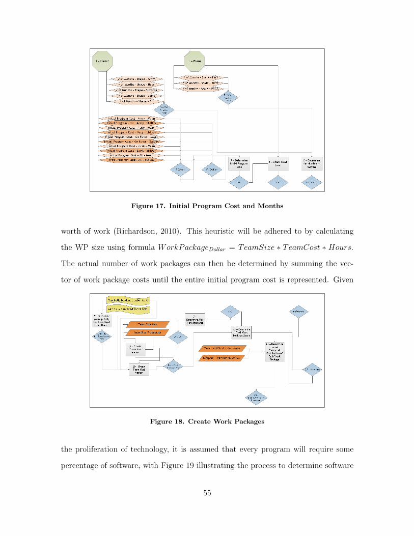
Figure 17. Initial Program Cost and Months

worth of work (Richardson, 2010). This heuristic will be adhered to by calculating

the WP size using formula WorkPackageDollar = TeamSize ∗ TeamCost ∗ Hours.

The actual number of work packages can then be determined by summing the vec-

tor of work package costs until the entire initial program cost is represented. Given

Figure 18. Create Work Packages

the proliferation of technology, it is assumed that every program will require some

percentage of software, with Figure 19 illustrating the process to determine software

55

impacts on the model. As the distribution of the percentage of the program that

requires software cannot be modeled due to lack of explicit reporting, a uniform dis-

tribution between 0 and 80% was used in an effort to reduce bias when choosing the

specific amount that any given program would have. This stochastically determined

software percentage was used in a binomial distribution creating a binary vector that

determines if a work package is software. The next step is to determine for those work

packages that are software, what is the amount of code growth that is likely to occur.

This vector of parameters is also stochastically determined based on a distribution

derived from the Holchin code growth study (2003). The output of this process is

illustrated in Table 11.

Table 11. Example of Software Designations

Work PackageNumber

Is Software Code GrowthPossible

Code Growth

1 1 0.3 0.32 1 0.21 0.213 0 0.64 04 1 0.82 0.825 0 0.47 06 0 0.39 07 1 0.53 0.538 0 0.61 09 1 0.76 0.7610 0 0.14 0

Drezner and Smith (1990) demonstrated that cost and schedule growth are cor-

related, leading to the creation of the delay cost factor illustrated in Figure 20. In

order to account for the specific programmatic hurdles that each system type faces,

it is hypothesized that the delay cost factor is based on the system type. The delay

cost factor parameters are determined based on the demographics of the iteration,

and then based on those parameters the delay cost factor is stochastically chosen.

56

Figure 19. Software Percentage

Through the iterative calibration process during initial model design, it was found

that this delay cost factor needed to be transformed by slight multiplication and ad-

dition in order to pass validation. The next step is to assign technology readiness

levels to each work package, as illustrated in Figure 21. Technology readiness levels,

or TRLs, have been used to describe the level of maturity that an element of a sys-

tem exhibits as defined in Table 12. Rodrigues (2000) demonstrated that lower TRL

levels correlated with cost and schedule slips, and are therefore likely to influence our

dependent variable of cost growth. In this model, TRL levels serve as a proxy for the

level of difficulty in accomplishing the work package. The TRLs assigned are based

57

Figure 20. Delay Cost Factor

58

on the demographic inputs of the phase of the program, as well as definitional inputs

that determine what technology readiness levels are acceptable for program initiation

(ASD R&E, 2013). Once the demographic check determines the appropriate range

of TRL values, a vector of technology readiness levels is stochastically chosen and

assigned to each work package.

Figure 21. Technology Readiness Level Distribution

Table 12. Technology Readiness Levels

TRL Definition9 Actual system proven through successful mission operations8 Actual system completed and qualified through test and demonstration7 System prototype demonstration in relevant environment6 System/subsystem model or prototype demonstration in relevant environment5 Component and/or breadboard validation in relevant environment4 Component and/or breadboard validation in laboratory environment3 Analytical and experimental critical function and/or characteristic proof of concept2 Technology concept and/or application formulated1 Basic principals observed and reported

Each work package is then temporally distributed across the number of months

that was determined previously. This temporal distribution is stochastically deter-

59

mined based on a truncated normal distribution which enables the characteristic

S-curve to take shape. A vector of temporal factors is then created which will cause

the work package to be delayed or moved forward in the schedule. This movement

direction is decided by the technology readiness level of work package. As the tech-

nology readiness levels for every phase are generally of range three, the middle value

will not move while the upper value, representing more mature technology, is likely

to be moved forward because it is easier. Those work packages with lower technology

readiness levels, representing less mature technology, are assumed to be more difficult

and therefore likely to be shifted to the right, taking longer.

At this point, the final cost for each work package, as well as the required time

to complete a work package, is determined. Each is a function of the time delay, the

time shift, and the software growth if any. If there is a delay or a stretch of the work

package, or if there is a shift forward in the schedule this will be calculated, resulting

in a determination of where each work package will end up in the temporal range.

For example a work package that was expected to be completed in period 10 but was

easier and therefore shifted left in the schedule could be expected to be completed in

period 7.

The next step is to create the hierarchy. At this point every work package has

been assigned initial cost and time distribution as well as a shifted cost and time

distribution. These work packages need to be aggregated in a series of parent-child

relationships until the Work Breakdown Structure (WBS) is formed (Richardson,

2010). To understand the parent-child relationships that form a WBS, consider the

construction of a house. ‘House’ is the parent, while ‘framing’, ‘plumbing’, ‘electrical’,

‘concrete’, etc., are the children. Children can be parents too, with ‘electrical’ being

a parent to ‘wiring’, ‘outlets’, ‘switches’, ‘fuses’, etc. as the children. This process

can continue until every nail of the house is accounted for as a child, and every child

60

Figure 22. Simplified Simulation Process Illustration

gets rolled up until there is only the final house. In order to create these parent-child

relationships, a vector of the number of children elements each parent element receives

is stochastically chosen, with the distribution of potential children per parent based on

observations within the CADE data. Using the house example again, the number of

children under the parent element ‘concrete’ will be relatively few, while the number

of children under the parent ‘plumbing’ will be more numerous. This assignment of

children elements to parents is carried out for every level, then each level is rolled

up and the process is repeated until there is only one element which represents the

entire program. In this way the hierarchical formulation of the C-CWBS will occur

until the sum of all work packages is represented at the highest WBS level (Fleming

61

& Koppelman, 2000). A simplified version of this hierarchical roll up is illustrated in

Table 13.

Table 13. Work Breakdown Structure Hierarchy Example

Element Names1 1.1 1.1.11 1.1 1.1.21 1.1 1.1.31 1.1 1.1.41 1.2 1.2.11 1.3 1.3.11 1.3 1.3.21 1.4 1.4.11 1.5 1.5.11 1.6 1.6.11 1.6 1.6.21 1.6 1.6.31 1.6 1.6.41 1.7 1.7.1

Element Dollar Values$1,000 $300 $125$1,000 $300 $25$1,000 $300 $100$1,000 $300 $50$1,000 $100 $100$1,000 $150 $85$1,000 $150 $65$1,000 $75 $75$1,000 $200 $200$1,000 $150 $30$1,000 $150 $40$1,000 $150 $25$1,000 $150 $55$1,000 $25 $25

At each level a name will be given stating the string of numbers that represent

the individual cell location. The cumulative sum at every level will also be taken.

This will create two matrices that represent the name or element location for every

work package at every level. At this point the earned value management artifacts

can be create. The first artifact, budgeted cost of work scheduled (BCWS), is simply

the initial work package cost placed in the original temporal distribution location.

The next artifact, budgeted cost of work performed (BCWP), is the initial work

package cost placed in the temporally shifted location, possibly spread over a number

of months if the work package was delayed. The final artifact, actual cost of work

performed (ACWP), is the work package final cost after accounting for time delay

62

costs as well as software growth costs if any, and this is placed in the temporally

shifted location.

Finally the top line data for the program contract can be created, and the earned

value management graph over time can also be plotted. An example of one of these

graphs is presented in Figure 23. This shows the characteristic S curves (Brown et.

al., 2015), as well as depicting program cost and schedule irregularities. This process

is then iterated for every demographic combination, at least 30 times, pursuant to the

central limit theorem. The naming convention for each program can be deciphered

0 10 20 30 40 50 60

020

0000

0060

0000

0010

0000

000

1_1_A_2_041_3_24

Month

Cos

t

ACWPBCWPBCWS

Figure 23. Earned Value Management Illustration

based on the following chart. As an example, the contract represented in Figure 23 is

an Army program, in EMD, for an aircraft system, using a Firm Fixed Price contract,

with an expected duration of 41 months, at a funding level making it an ACAT 3

program, with 24% of the program revolving around software.

63

Table 14. Contract Naming Convention

Variable LevelsLead Branch 1 - Army

2 - Navy3 - Air Force4 - Joint

Contract Phase 1 - EMD2 - RDTE3 - Production

System Type A - Aircraft SystemB - Electronic SystemC - Missile SystemD - OrdinanceE - Sea SystemsF - Space SystemG - Surface VehicleH - Unmanned Air SystemI - Unmanned Maritime SystemJ - Launch VehicleK - Automated Information SystemL - Common Elements

Contract Type 1 - Cost Plus2 - Firm Fixed Price3 - Fixed Price Incentive

Duration in Months Continuous - Rounded to MonthACAT Level 1 - ACAT I

2 - ACAT II3 - ACAT III

Percent Software Continuous - Rounded to Percent

Model Validation.

The proposed validation methodology will attempt to validate that the simulation

models the population characteristics of contract cost growth. This validation will be

accomplished by conducting a t-test at α = 0.05 showing that the range of percent of

contract cost increase from the modeled programs is not statistically different than

64

the range of contract cost increase observed in the sample set. This will demonstrate

that as a whole, the randomly generated program files match the distribution of cost

increases observed in the observed programs from the CADE database.

4.3 Results

The distribution of the dependent variable “Percent Budget Increase” for both

the generated data set and the CADE data set can be seen in Figure 24. While not

identical, the mean and range closely resemble each other, and performing a two-tailed

t-test with α = 0.05 results in p − value = 0.8734 as seen in Figure 25, indicating

that the means of the two data sets is not significantly different. As the range and

distribution are similar, the generated data set passes the analysis of means criteria

for validation as a population.

Figure 24. Boxplot Results

65

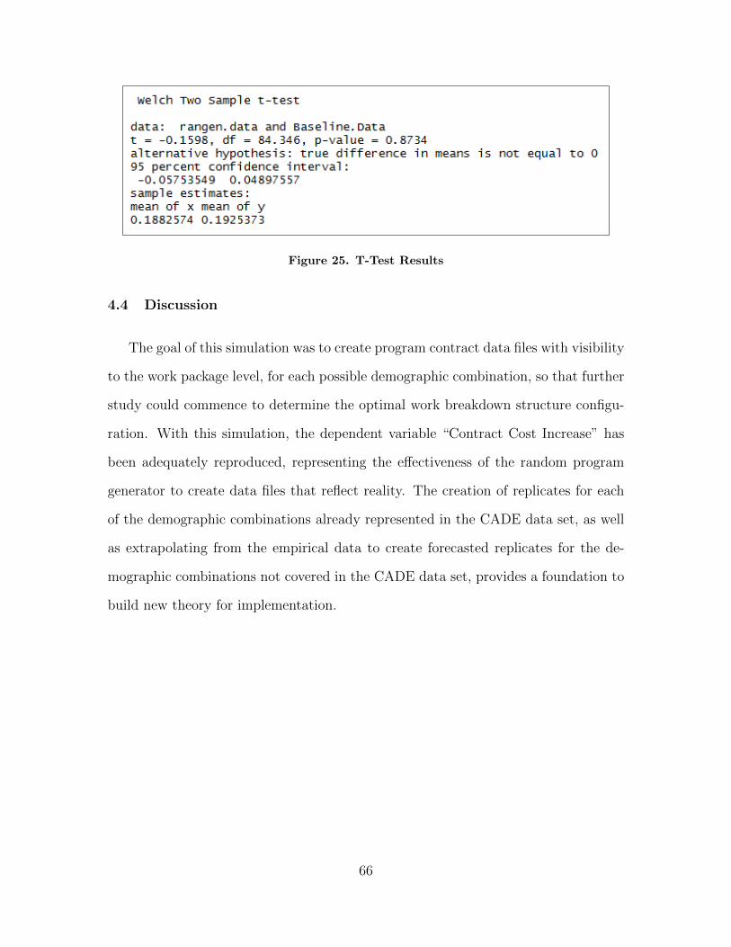
Figure 25. T-Test Results

4.4 Discussion

The goal of this simulation was to create program contract data files with visibility

to the work package level, for each possible demographic combination, so that further

study could commence to determine the optimal work breakdown structure configu-

ration. With this simulation, the dependent variable “Contract Cost Increase” has

been adequately reproduced, representing the effectiveness of the random program

generator to create data files that reflect reality. The creation of replicates for each

of the demographic combinations already represented in the CADE data set, as well

as extrapolating from the empirical data to create forecasted replicates for the de-

mographic combinations not covered in the CADE data set, provides a foundation to

build new theory for implementation.

66

Bibliography

1. Assistant Secretary of Defense for Research and Engineering (2013). Technology

Readiness Assessment Guidance (TRA Guide). Washington, DC: U.S. Government

Printing Office.

2. Barraza, G. A., Back, W. E., & Mata, F. (2000). Probabilistic monitoring of

project performance using SS-curves. Journal of Construction Engineering and

Management, 126(2), 142-148.

3. Barraza, G. A., Back, W. E., & Mata, F. (2004). Probabilistic forecasting of project

performance using stochastic S curves. Journal of Construction Engineering and

Management, 130(1), 25-32.

4. Blickstein, I., Boito, M., Drezner, J. A., Dryden, J., Horn, K., Kallimani, J. G.,

Libicki, M. C., McKernan, M., Molander, R.C., & Nemfakos, C. (2011). Root

Cause Analyses of Nunn-McCurdy Breaches, Volume 1: Zumwalt-Class Destroyer,

Joint Strike Fighter, Longbow Apache and Wideband Global Satellite. RAND

National Defense Research Institute Santa Monica CA.

5. Brown, G. E., White, E. D., Ritschel, J. D., & Seibel, M. J. (2015). Time Phasing

Aircraft R&D Using the Weibull and Beta Distributions. Journal of Cost Analysis

and Parametrics, 8(3), 150-164.

6. Colin, J., and Vanhoucke, M. (2014). Setting Tolerance Limits for Statistical

Project Control Using Earned Value Management. Omega - International Jour-

nal of Management Science, 49, 107-122.

7. Department of Defense (2011). Department of Defense Standard Practice Work

Breakdown Structures for Defense Materiel Items (MIL-STD-881C). Washington,

DC: U.S. Government Printing Office.

67


schedules (No. RAND/R-3937-ACQ). RAND CORP SANTA MONICA CA.

9. Fitzpatrick, B., Meyer, S., & Stubbs, J. (2016). Introducing a Metric to Quantify

Work Breakdown Structure Effectiveness. Unpublished.

10. Fitzpatrick, B., White, E., Lucas, B., & Elshaw, J. (2016). Alternative For-

mulation of a Pessimistic Estimate at Completion. Journal of Cost Analysis and

Parametrics, Submitted, pending acceptance.



12. Goh, A. T. C. (1995). Back-propagation neural networks for modeling complex

systems. Artificial Intelligence in Engineering, 9(3), 143-151.

13. Gounatidis, N. (2006). How Does the Political Nature of the Defense Acquisition

Process Affect Cost Growth (No. AFIT/GCA/ENV/06-01S). Air Force Institute

of Technology Wright-Patterson AFB OH Graduate School of Engineering and

Management.

14. Government Accountability Office/National Security and International Affairs

Division (1992). Events Surrounding the Navy’s A-12 Aircraft Program. (GAO

Publication No. 92-190FS). Washington, D.C.: U.S. Government Printing Office

15. Gunther, F., & Fritsch, S. (2010). neuralnet: Training of neural networks. The R

Journal, 2(1), 30-38.

16. Holchin, B. (2003). Code Growth Study. Goleta, CA: Tecolote Research, Inc.



68


ing and Management.




19. Kennedy, M. C., & O’Hagan, A. (2001). Bayesian calibration of computer models.

Journal of the Royal Statistical Society. Series B, Statistical Methodology, 425-464.

20. Leonard, R. S., & Wallace, A. (2014). Air Force Major Defense Acquisition Pro-

gram Cost Growth Is Driven by Three Space Programs and the F-35A: Fiscal

Year 2013 President’s Budget Selected Acquisition Reports. Santa Monica, Calif.:

RAND Corporation, RR-477-AF.



22. Rodrigues, L. R. (2000). Joint strike fighter acquisition: Development schedule

should be changed to reduce risks (No. GAO/T-NSIAD-00-132). General Account-

ing Office Washington DC National Security and International Affairs Division.





24. Ruter, I. I., & Philip, E. (2007). Cost Growth in Weapons Systems: Re-examining

Rubber Baselines and Economic Factors (No. AFIT/GCA/ENV/07-M9). Air Force


ing and Management.

69

25. Smirnoff, J. P., & Hicks, M. J. (2008). The impact of economic factors and acquisi-

tion reforms on the cost of defense weapon systems. Review of Financial Economics,

17(1), 3-13.

26. Sullivan, M. J. (2011). DOD COST OVERRUNS: Trends in Nunn-McCurdy

Breaches and Tools to Manage Weapon Systems Acquisition Costs (No. GAO-

11-499T). Government Accountability Office Washington DC.

27. Under Secretary of Defense for Acquisition, Technology, and Logistics (2015).

Operation of the Defense Acquisition System (DODI 5000.02). Washington, DC:

U.S. Government Printing Office.

28. Werbos, P. J. (1988). Generalization of backpropagation with application to a

recurrent gas market model. Neural Networks, 1(4), 339-356.

70

V. Determining The Optimal Work Breakdown Structure

5.1 Introduction

Defense acquisition programs are amazingly complex, and in order to manage these

programs a large number of tools have been created that assist decision-makers. The

cost and schedule control tool, Earned Value Management (EVM), has been mandated

and implemented on a large number of DOD programs. The specific implementation,

driven by the granularity of the government contract work breakdown structure (G-

CWBS), is left to government program managers (PM) who have little guidance on

the most effective G-CWBS implementation. This lack of guidance has fueled an

ongoing search for an optimal level of WBS detail.

Previous qualitative analysis by Bushey (2007) and Thomas (1999) investigated

the implementation of reporting policy and presented conceptual frameworks for more

useful implementation. Bushey describes the appropriate level of breakout in qual-

itative terms, noting that an effective cost reporting structure requires flexibility to

enable various forms of analysis. EVM practiced only at the top line program level

does not provide this flexibility, because there is no ability to determine root-causes

of issues with such a high level data point. He goes on to propose a WBS structure

down to the Work Package level, as this will allow identification of root causes in

cost and schedule discrepancies, and facilitate discussions with the Control Account

Managers (CAMs) who are in a position to provide information and alternative action

recommendations to the government PM. This recommendation is absolutely correct

within the vacuum of a desire for visibility. It is not, however, practical, and does

not consider the benefits to the flexibility enjoyed by the contractor by being able to

modify individual work packages without going through the bureaucratic maneuvers

necessary to modify the Government Contract WBS. The implementation of report-

71

ing at the Work Package level would increase the reporting burden on the contractor,

as well as require contractual approval or language for every minor modification, both

of which would increase the cost to the government.

Thomas provides an in-depth review of the literature surrounding the creation and

implementation of the regulation requiring EVM, and attempts to determine if the

policies it contains actually impede acquisition reform initiatives and a PM’s ability to

manage. He bases his findings, that the policy does in fact hinder acquisition reform

initiatives and program management, on personal experience and interviews with

government and contractor personnel. He posits that a WBS prepared in accordance

with MIL-HBK-881 will not provide sufficient insight into many of the elements.

The concept that limiting reporting at too broad a level will inhibit a PM’s ability

to manage is not controversial, but this scenario is only likely if the PM does the

minimum required by the MIL-HBK-881. The actual policy directs the PM to ensure

that their WBS is broken out to sufficient detail to allow visibility. What seems to

be lacking in the PM community is a method for determining when sufficient detail

has been achieved, or when further break-out is required.

Previous quantitative research has not been able to adequately provide broad

guidance either. Studies have found within certain program types that a single ele-

ment is predictive of cost growth at lower than WBS Level 1 (Rosado, 2011), that

elemental WBS Level 5 data is no better than elemental WBS Level 3 data (John-

son, 2014), and that lower level WBS data does not improve EAC forecast accuracy

(Keaton, 2015). These mixed findings were not generalizable outside of the specific

areas of data availability that constrained each research effort, leaving the need for

an objective way to determine an optimal level of WBS detail unanswered.

72

New Tools Have Been Introduced.

EVM has recently been updated with an alternative estimate at completion (EAC)

calculation method (Fitzpatrick, White, Lucas, & Elshaw, JCAP 2016). Using this

alternative EAC calculation, a pessimistic estimate for every leaf element of a WBS

can now occur, which enabled the creation of a new metric. The G-Score introduced

by Fitzpatrick, Meyer, and Stubbs (2016), is a quantitative measure that can be

used to judge the level of granularity inherent in a given G-CWBS. The G-Score

was empirically shown to be a significant explanatory variable when used to forecast

contract cost growth from time 0, using only demographic descriptors and information

known at the time of contract award. This demonstration, while beneficial, was

inherently reactive in nature, as it was used with the firmly entrenched WBS of the

historical programs in their data set. A proactive use, the trade-off analysis and

design calibration of the work breakdown structure, would provide a tool that helps

inform program management decisions on the level of granularity to request from the

contractor, before contract award.

A G-score could be calculated for any proposed WBS that is developed providing

a way to grade different structural choices. The benefit derived from this is that the

program manager would have better understanding of the granularity that the vari-

ous work breakdown structures under review are capable of. Coupled with a cost to

implement each proposed WBS, a cost per level of granularity could be constructed.

For example a WBS broken out simply to Level 3 may cost $500,000 to implement.

Another WBS broken out to a fine level of granularity such that no leaf element

represents more than 1% of the work to be performed, might cost $5 million to imple-

ment. A third WBS, broken out so that no leaf element would represent more than

4% of work to be performed might cost $1 million to implement. The corresponding

G scores for these three WBS constructs might be 0.1, 0.8, and 0.6, which yields a

73

corresponding cost per level of granularity of 0.2, 0.16, and 0.6. In this simple exam-

ple is easy to see that the option which breaks out the WBS to the 4% level gives

the greatest value by enabling significant granularity for a reasonable cost. While the

WBS broken out to the 1% level offers the most granularity, the cost to implement

such a reporting scheme reduces the overall value.

Program Management Apprehension.

Forecasts provided by previously available EVM tools have been disregarded in

the past, with Christensen finding that information which may jeopardize the project

is sometimes discarded in favor of more optimistic, but less accurate forecasts (Chris-

tensen, 1996). This notion is generally supported by the work of Niskanen, who

posited that the goal of bureaucrats is to maximize their budget, and would therefore

prefer to be rationally ignorant to anything that might reduce their budget (Niska-

nen, 1975). Another body of work that supports Christensen’s findings is Herzberg’s

Motivation and Hygiene Theory (MHT). The MHT or the two-factor theory of job

satisfaction, posits that employee satisfaction and dissatisfaction can be measured

on two separate continuum. The motivation factors that influence job satisfaction

are intrinsic factors such as achievement, advancement, responsibility, recognition,

and the work itself. Hygiene factors affecting dissatisfaction are extrinsic factors

such as company policy, salary, work conditions, and supervision (Stello, 2011). A

study comparing employees of private and public organizations empirically found that

public employees were more influenced by intrinsic factors, while private sector em-

ployees reported that extrinsic factors more heavily influenced their job satisfaction

(Maidani, 1991). A specific school of thought argues that intrinsically or extrinsi-

cally motivated individuals self select themselves into the public or private sector

(Christensen & Wright, 2011), however the available incentives of each sector provide

74

an explanation as well. In the private sector, financial rewards and salary increases

are justified by increased revenues generated, whereas the public sector is limited

in financial reward options, and salaries are dictated by public law. This difference

in available incentives matches very well with the difference in satisfaction factors

previously found (Maidani, 1991), which further supports Christensen’s findings by

illustrating how the incentives that drive government program managers cause them

to focus on achieving program approval, and not necessarily on the most efficient use

of information if it threatens to disrupt their program.

Identify The Paradigms.

Understanding that program managers have an incentive to see their program

succeed, it will be useful to understand the utility that PMs would find in imple-

menting the G-Score. There are two PM perspectives that need to be addressed

when applying decision analysis to determine the optimal level of WBS breakout.

The previously reviewed research makes it dubious to assume that decision makers

will work to maximize the public monetary utility. It is more likely that they will

endeavor to maximize their personal utility, not measured in salary which will re-

main constant based on statute, but in other factors. The two measures that will be

used are management utility, and budget utility. Management utility is the benefit

that the program manager receives from implementing their chosen WBS structure.

This utility is quantified using the G-Score, with higher G-Scores corresponding to

higher utility due to the increased granularity with which they will be able to manage

their program. Budget utility is the intangible benefit that they receive from being in

charge of the program, and the corresponding increase in their budget. An increase in

the manager’s budget is seen as an increase in utility, with the corollary that program

cancellation, or reductions in appropriations results in lower utility.

75

Finally, there is a third perspective; that of the general public, and the concern for

the best use of appropriated funds. This perspective is public utility, or the benefit

that the public receives from efficiently executed programs. Public utility corresponds

with the generally understood concept that having more money is desirable, and

having less money is not desirable. From this perspective, program completion on

budget provides maximum utility, while being over budget reduces utility as there is

less money for other priorities.

Purpose of Study.

The purpose of this study is to generate an optimal G-CWBS from a variety of

Work breakdown structures, from management, budget, and public utility perspec-

tives. The optimal structures will then be compared and analyzed. The results from

the management utility perspective will provide an answer to the initial question

surrounding optimal WBS breakdown, while the results from the budget and public

utility perspectives, and their delta, if any, from the management optimal structure,

will be analyzed for any interesting insights.

5.2 Methodology

General Description of Utility Theory Process.

In order to determine the optimal structure, utility theory decision trees will be

used for each perspective. The simplified process of using a decision tree contains

two node types, decision and probabilistic, to illustrate all possible occurrences, and

provide a probability of each occurrence happening. There will only be one decision

node on the tree presented, and that will be the decision of the WBS structure. The

rule for deciding the structure is to choose the path that has the highest expected

utility. In most instances, utility is measured in dollars, however in the case of

76

the management utility calculation, the G-Score will be the unit of measure. An

axiom of utility theory is that more utility is always preferable to less (Neumann &

Morgenstern, 1953) , so the optimal WBS structure for each perspective will be that

choice which has the maximum utility, in whatever unit space that perspective is.

The uncertainty involved in the decision tree will occur in two places. The first

will be the probability that adverse action will occur. Adverse action can take one of

4 forms: Project cancellation, major reduction, medium reduction, or low reduction.

It is hypothesized that the likelihood of adverse action increases exponentially as a

program goes over budget, with the logic being that a small amount over budget

will not likely result in program cancellation, but will likely lead to low reduction,

whereas a major overage will very likely lead to a reduction, and may lead to program

cancellation. A budget overage that will trigger adverse action is defined as an increase

of 25% over expected, which is based on the threshold of a Nunn-McCurdy breach.

Specific probability of adverse action is based on the curve and formula illustrated in

Figure 26.

The budget overage is based on an estimated EAC using the linear regression

model proposed previously proposed (Fitzpatrick, Meyer, & Stubbs 2016). This is

based on the G-Score available at time 0, and would give the PM a good feel for if the

program is likely to go over budget. Depending on the perspective, the value of this

information will change, because if the estimate forecasts significant cost growth, the

program may be canceled or stalled for more research. This outcome is desirable for

the public utility, but undesirable for the PM’s budget utility. Management utility

is indifferent to this outcome, as its utility is based on the G-Score and the related

granularity.

The probability of adverse action was modeled as an exponential function as seen

in Equation 30. J and K represent constants parameters that ensure that the proba-

77

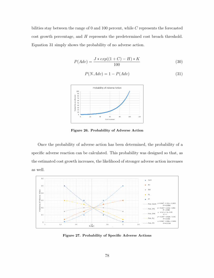
bilities stay between the range of 0 and 100 percent, while C represents the forecasted

cost growth percentage, and H represents the predetermined cost breach threshold.

Equation 31 simply shows the probability of no adverse action.

P (Adv) =J ∗ exp((1 + C)−H) ∗K

100(30)

P (N.Adv) = 1− P (Adv) (31)

Figure 26. Probability of Adverse Action

Once the probability of adverse action has been determined, the probability of a

specific adverse reaction can be calculated. This probability was designed so that, as

the estimated cost growth increases, the likelihood of stronger adverse action increases

as well.

Figure 27. Probability of Specific Adverse Actions

78

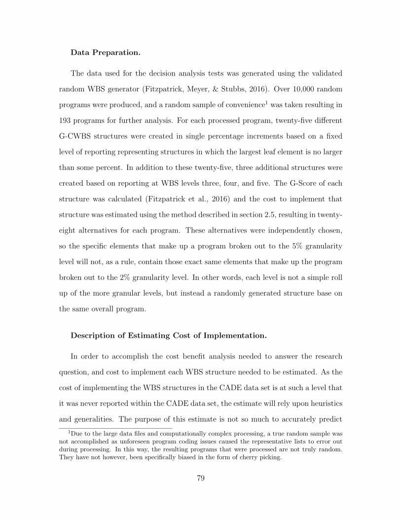
Data Preparation.

The data used for the decision analysis tests was generated using the validated

random WBS generator (Fitzpatrick, Meyer, & Stubbs, 2016). Over 10,000 random

programs were produced, and a random sample of convenience1 was taken resulting in

193 programs for further analysis. For each processed program, twenty-five different

G-CWBS structures were created in single percentage increments based on a fixed

level of reporting representing structures in which the largest leaf element is no larger

than some percent. In addition to these twenty-five, three additional structures were

created based on reporting at WBS levels three, four, and five. The G-Score of each

structure was calculated (Fitzpatrick et al., 2016) and the cost to implement that

structure was estimated using the method described in section 2.5, resulting in twenty-

eight alternatives for each program. These alternatives were independently chosen,

so the specific elements that make up a program broken out to the 5% granularity

level will not, as a rule, contain those exact same elements that make up the program

broken out to the 2% granularity level. In other words, each level is not a simple roll

up of the more granular levels, but instead a randomly generated structure base on

the same overall program.

Description of Estimating Cost of Implementation.

In order to accomplish the cost benefit analysis needed to answer the research

question, and cost to implement each WBS structure needed to be estimated. As the

cost of implementing the WBS structures in the CADE data set is at such a level that

it was never reported within the CADE data set, the estimate will rely upon heuristics

and generalities. The purpose of this estimate is not so much to accurately predict

1Due to the large data files and computationally complex processing, a true random sample wasnot accomplished as unforeseen program coding issues caused the representative lists to error outduring processing. In this way, the resulting programs that were processed are not truly random.They have not however, been specifically biased in the form of cherry picking.

79

costs in the real world, but instead provide a defensible, constant, and reproducible

estimate for each of the potential WBS structures, so that comparisons can be made.

A crosscheck will also be used based on the Cooper & Lybrand (1994) study that

gives a ballpark range for the cost of reporting as a percent of total cost.

The characteristics that the estimate should have: As more detailed data is re-

quired, the cost of reporting goes up. The cost increase should not behave linearly

with regard to the level of reporting, as the element parent-child relationship would

cause expected exponential growth. The primary cost driver in reporting is the cre-

ation of the initial reporting system that is agreed upon. It is not assumed that an

individual is starting from scratch from each report, but instead is simply turning the

handle on a piece of software that was created specifically for the program that is be-

ing reported. This indicates that the majority of reporting costs is actually software

cost.

The estimate is a simple Cost Estimating Relationship (CER) that states for

every y = (30 + x) ∗ 2000 where y is the cost to implement, and x is the number of

leaf elements plus parent elements that exist in the WBS structure being considered.

The parameter 2000 represents an unattributable heuristic of $2000 per line of code

that the authors have previously used in the field. The parameter 30 represents

the assumed wrap code that any report would require regardless of the number of

individual report elements. It is expected that each reported element requires a

line of code to search and sum, and that these lines of code would be added to the

wrap code, and multiplied by the cost per line. While this is a very simplistic and

undoubtedly flawed approach, this estimation technique produced costs that were

comparable to the mean cost of 0.9% of total program cost that Cooper & Lybrand

reported in their survey, as illustrated in Figure 28. Additionally it satisfies all desired

attributes, creating estimated costs that grew exponentially in accordance with leaf

80

element proliferation, and as such was found acceptable for creating the comparative

costs for use in decision analysis.

Figure 28. Cost to Implement Status Quo Level of Reporting in Generated Programs

Utility Multipliers.

Each potential outcome was given a utility multiplier to reduce expected utility

for anything other than full funding as illustrated in Table 15. Management and

Public utility multipliers are identical, based on the assumption that a relatively

stable decline in utility will be expected as the magnitude of an adverse action to

the program increases. For example, the utility of the G-Score is reduced to 0 if the

program is canceled, as there will be nothing left to manage. Similarly, the public will

81

receive no utility from a program that gets canceled. As the adverse actions become

less severe, the reduction in utility becomes less severe as well. A program that

has been subjected to congressional oversight, budget reductions, and the associated

schedule delays, will nevertheless produce utility, however not nearly as much as a

program executed to plan. Budget utility, serving as the proxy for the PM’s budget

maximizing incentives, is more variable. This is based on the assumption that a

program cancellation or severe budget reductions would provide negative utility, due

to the aura of management failure associated with failed programs. Conversely, low to

medium reductions, while reducing the PM’s budget, are fairly common and therefore

don’t also carry the stigma of severely reduced programs. Finally, full funding provide

maximum utility for the budget maximizing program manager.

Table 15. Utility Multipliers

Program

Cancel

Reduction

(High)

Reduction

(Medium)

Reduction

(Low)

Full

Funding

Management Utility 0.0 0.2 0.5 0.8 1.0

Budget Utility -0.2 -0.1 0.3 0.6 1.0

Public Utility 0.0 0.2 0.5 0.8 1.0

Description of Budget Utility Curve Formulation.

Two assumptions were made when determining the PM’s budget utility curve.

The first is that the PM finds greater utility with a greater budget, and less utility

from a smaller budget. This is based on the motivation factors leading to a desire

to maximize their budget. The second assumption is that the decision maker is risk

averse, which has been empirically shown to be likely (MacCrimmon, 1968).

82

The equation used to calculated the utility function for the PM is illustrated as

Equation 32, where a is equal to the minimum possible utility value, b represents

the maximum possible utility value, and R represents a risk tolerance parameter

constant. In this scenario, the maximum and minimum utility values are based on

the percentage of the PM’s portfolio that the current contract represents, and the

the x value represents the base budget utility of the current WBS option. The curves

illustrated in Figure 29 show that as the current contract represents a greater share

of the PM’s total portfolio, the potential utility of the contract rises as well. If they

only have one program, the utility to them of that one program is very high, but

if they have many programs, the utility of the single program under review is much

less. The various curves illustrate that as risk aversion increases, the utility of any

program increases, with the loss of the program representing a greater loss of utility

than if the decision maker was risk neutral.

U(x) =

1− exp(

−(x−a)R

)

1− exp(

−(b−a)R

)

(32)

Description of Management Utility Curve Formulation.

The management utility function is quantified as the specific G-Score divided

by the cost to implement the proposed work breakdown structure multiplied by the

initial program cost (IPC), as illustrated in Equation 33. The fraction of G-Score

to implementation cost provides the benefit to cost ratio, while the IPC acts as a

scalar to magnify the differences between the different WBS implementations and

corresponding G-Scores. As described in the introduction, the WBS that provides

the best G-Score to cost ratio will be chosen as the structure providing the most

management utility.

83

Figure 29. PM Budget Utility by Contract % of Portfolio at Different Risk Tolerances

U(x) = (G− Score/Cost To Implement) ∗ Initial Program Cost (33)

Description of Public Utility Curve Formulation.

The public utility curve is simply the IPC multiplied by the utility multipliers

in Table 15. This is based on the notion that public only cares about the outcome,

and an efficient path to that outcome. Full utility occurs when no adverse actions

are taken; no utility occurs if the program gets canceled, and utility is reduced if the

program gets delayed or comes in over budget.

84

Description of the Decision Tree Tool.

Figure 30 is a simplified illustration of the decision tree that was created to de-

termine the optimal work breakdown structure for each paradigm. While Figure 30

has 6 decision paths (paths that originate from a rectangle), the actual decision trees

had 28 decision paths. 25 of the paths lead to work breakdown structures that had a

maximum percentage size of the largest leaf element, incremented in single percentage

points. The top four decision paths in the example lead to WBSs where the largest

leaf element represents no more than 1%, 3%, 5%, or 9% of the total program cost,

respectively. The remaining 3 options were WBSs that were designed to report at a

specific WBS level, with Level 3 and Level 4 options illustrated.

For each WBS, an estimate at completion based on the G-Score was used to pop-

ulate the uncertainty node (represented by a circle in the tree), with the probability

of adverse action illustrated in Figure 26 previously. For either adverse action, or not

adverse action, there are 5 possible outcomes: Cancellation, Large Budget Reduction,

Medium Budget Reduction, Small Budget Reduction, and Full Funding. The prob-

abilities of each of theses were illustrated in Figure 27. At this point, a probability

of occurrence has been calculated for each potential outcome. The expected utility

of each outcome, calculated using the methods described for each utility perspective,

are then multiplied by the probability of occurrence. These weighted expected utility

values are then summed until there is one value for each decision path. The decision

path with the highest expected utility value is then chosen as the optimal solution.

This process produced three distinct optimal WBS structures for each program based

on the utility perspective.

85

Choose Which Reporting Structure

To Implement

Adverse

Adverse

Adverse

Adverse

Adverse

Adverse

Specific Action

Specific Action

Specific Action

Specific Action

Specific Action

Specific Action

Specific Action

Specific Action

Specific Action

Specific Action

Specific Action

Specific Action

P.Adv

P.N.Adv

P.Adv

P.N.Adv

P.Adv

P.N.Adv

P.Adv

P.N.Adv

P.Adv

P.N.Adv

P.Adv

P.N.Adv

WBS Structure – Maximum Leaf <= 1% of Total Program Cost




WBS Structure – Level 3 Reporting

WBS Structure – Level 4 Reporting

Figure 30. Simplified Decision Tree

5.3 Results

The optimal WBS structure results from a management utility perspective is

shown in Figure 31. The range of G-Scores achieved by these structures is shown in

Figure 33, while the range of costs to implement these structures is shown in Figure

34. These figures illustrate that from a program visibility and control perspective,

there is no single “best” structure. While the status quo, reporting at WBS level 3, is

the conspicuous mode of the data set, every other possible structure was optimal at

least once, with most hovering around 5 programs. This greatly illustrates the cliche

answer “It Depends”. Other insights, the average G-Score achieved by these optimal

structures was 0.178, with an average cost to implement hovering around $0.9M.

The optimal WBS structure results from a program manager’s budget utility per-

spective is shown in Figure 35. The range of G-Scores achieved by these structures is

shown in Figure 37, while the range of costs to implement these structures is shown

86

Figure 31. Management Utility Optimal Structure Choices

Figure 32. Management Utility Optimal Structure Choices - Binned

in Figure 38. There appears to be a bimodal distribution with optimal scenarios

clustered around the status quo, and around small percentage granularization. Other

insights, the average G-Score achieved by these optimal structures was 0.19, with an

average cost to implement of $2.6M.

87

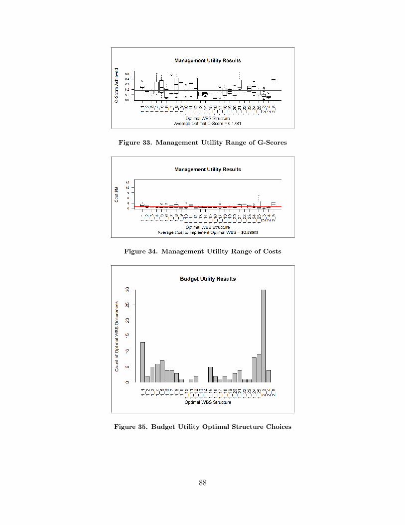
Figure 33. Management Utility Range of G-Scores

Figure 34. Management Utility Range of Costs

Figure 35. Budget Utility Optimal Structure Choices

88

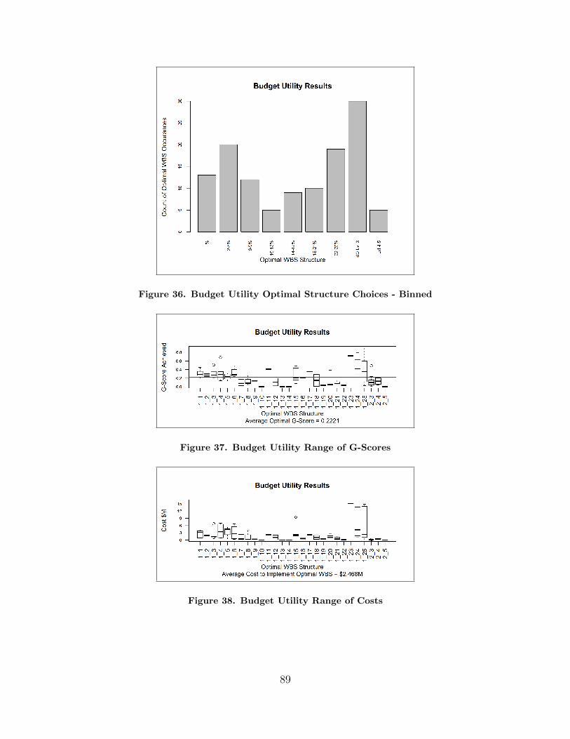
Figure 36. Budget Utility Optimal Structure Choices - Binned

Figure 37. Budget Utility Range of G-Scores

Figure 38. Budget Utility Range of Costs

89

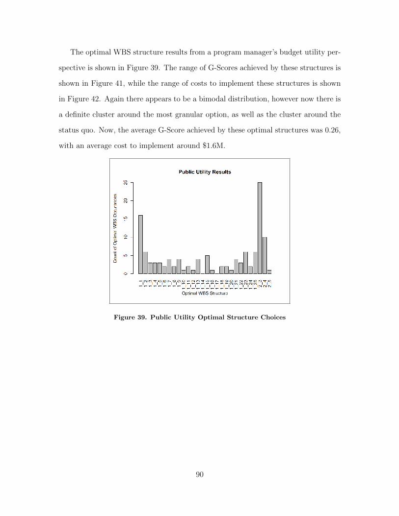
The optimal WBS structure results from a program manager’s budget utility per-

spective is shown in Figure 39. The range of G-Scores achieved by these structures is

shown in Figure 41, while the range of costs to implement these structures is shown

in Figure 42. Again there appears to be a bimodal distribution, however now there is

a definite cluster around the most granular option, as well as the cluster around the

status quo. Now, the average G-Score achieved by these optimal structures was 0.26,

with an average cost to implement around $1.6M.

Figure 39. Public Utility Optimal Structure Choices

90

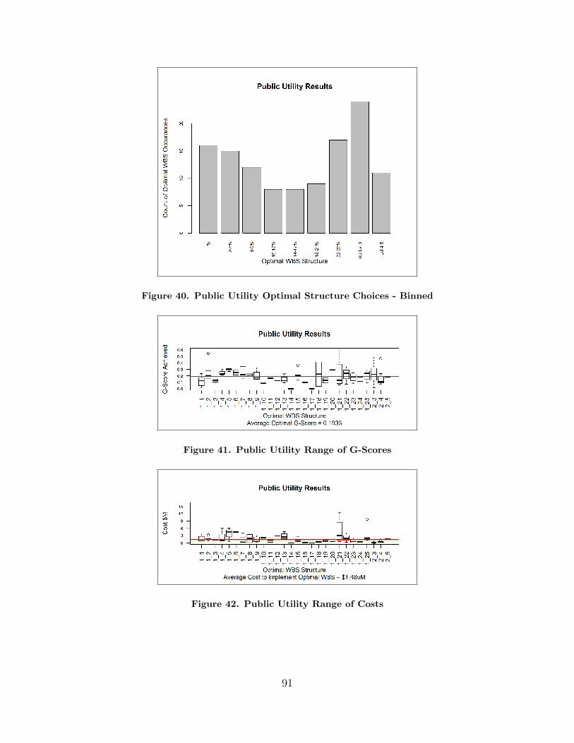
Figure 40. Public Utility Optimal Structure Choices - Binned

Figure 41. Public Utility Range of G-Scores

Figure 42. Public Utility Range of Costs

91

5.4 Discussion

The results presented clearly confirm the notion that, without any guidance or

information, the status quo of reporting at WBS level 3 is the most often occurring

single WBS structure, regardless of utility perspective. On the other hand, Figures

43, 44, and 45 illustrate that in a binary match-up of the Status Quo: WBS Level 3,

or any alternative, the alternative option wins hands down.

Figure 43. Management Utility Comparison of Status Quo against Alternative Struc-

tures

It is also important to note that when the PM’s incentive was to increase their

budget, the average cost spent on the optimal structure was higher than the other

two perspective. Similarly, when the perspective’s incentive was to increase program

management, G-Scores were higher. From the public perspective, there seemed to be

a desire for either the cheapest, or the most granular and often the most expensive

reporting option.

The programs investigated had a representative range of cost overruns. It is

hypothesized that those programs with large cost overruns justified the increased

92

Figure 44. Budget Utility Comparison of Status Quo against Alternative Structures

Figure 45. Public Utility Comparison of Status Quo against Alternative Structures

expense in granularity level, whereas those programs that did not experience cost

growth did not justify the expense.

The bottom line is that all program would benefit from a more tailored approach

to WBS structure formulation, and that the G-Score now provides a method to quan-

93

titatively compare different structures. The program manager will still need to un-

derstand their program’s strengths and weaknesses enough to know whether they will

benefit from the additional insights greater granularity would provide, or if the pro-

gram is low risk enough that the additional expense of a more granular WBS is not

worth it.

94

Bibliography



2. Christensen, R. K., & Wright, B. E. (2011). The Effects of Public Service Mo-

tivation on Job Choice Decisions: Disentangling the Contributions of Person-

Organization Fit and Person-Job Fit. Journal of public administration research

and theory, 21(4), 723-743.

3. Christensen, D. S. (1996). Project advocacy and the estimate at completion prob-

lem. The Journal of Cost Analysis, 13(1), 35-60.

4. Coopers & Lybrand with TASC, Inc. (1994). The DoD Regulatory Cost Premium:

A Quantitative Assessment, annotated briefing prepared for Secretary of Defense

William Perry.

5. Fitzpatrick, B., Meyer, S., & Stubbs, J. (2016). Introducing a Metric to Quantify

Work Breakdown Structure Effectiveness. Unpublished.

6. Fitzpatrick, B., White, E., Lucas, B., & Elshaw, J. (2016). Alternative Formulation

of a Pessimistic Estimate at Completion. Journal of Cost Analysis and Parametrics,

Submitted, pending acceptance.

7. Fitzpatrick, B., White, E., Lucas, B., & Elshaw, J. (2016). Generating Random

DoD Program Data. Journal of Simulation. Unpublished.




ing and Management.

95




10. MacCrimmon, K. R. (1968). Descriptive and normative implications of the

decision-theory postulates. In Risk and uncertainty (pp. 3-32). Palgrave Macmillan

UK.

11. Maidani, E. A. (1991). Comparative study of Herzberg’s two-factor theory of

job satisfaction among public and private sectors. Public Personnel Management,

20(4), 441-448.

12. Neumann, J. V., & Morgenstern, O. (1953). Theory of games and economic be-

havior.

13. Niskanen, W. A. (1975). Bureaucrats and politicians. The Journal of Law &

Economics, 18(3), 617-643.





15. Stello, C. M. (2011). Herzberg’s two-factor theory of job satisfaction: An inte-

grative literature review. In Unpublished paper presented at The 2011 Student

Research Conference: Exploring Opportunities in Research, Policy, and Practice,

University of Minnesota Department of Organizational Leadership, Policy and De-

velopment, Minneapolis, MN.



96

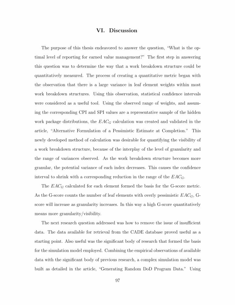
VI. Discussion

The purpose of this thesis endeavored to answer the question, “What is the op-

timal level of reporting for earned value management?” The first step in answering

this question was to determine the way that a work breakdown structure could be

quantitatively measured. The process of creating a quantitative metric began with

the observation that there is a large variance in leaf element weights within most

work breakdown structures. Using this observation, statistical confidence intervals

were considered as a useful tool. Using the observed range of weights, and assum-

ing the corresponding CPI and SPI values are a representative sample of the hidden

work package distributions, the EACG calculation was created and validated in the

article, “Alternative Formulation of a Pessimistic Estimate at Completion.” This

newly developed method of calculation was desirable for quantifying the visibility of

a work breakdown structure, because of the interplay of the level of granularity and

the range of variances observed. As the work breakdown structure becomes more

granular, the potential variance of each index decreases. This causes the confidence

interval to shrink with a corresponding reduction in the range of the EACG.

The EACG calculated for each element formed the basis for the G-score metric.

As the G-score counts the number of leaf elements with overly pessimistic EACG, G-

score will increase as granularity increases. In this way a high G-score quantitatively

means more granularity/visibility.

The next research question addressed was how to remove the issue of insufficient

data. The data available for retrieval from the CADE database proved useful as a

starting point. Also useful was the significant body of research that formed the basis

for the simulation model employed. Combining the empirical observations of available

data with the significant body of previous research, a complex simulation model was

built as detailed in the article, “Generating Random DoD Program Data.” Using

97

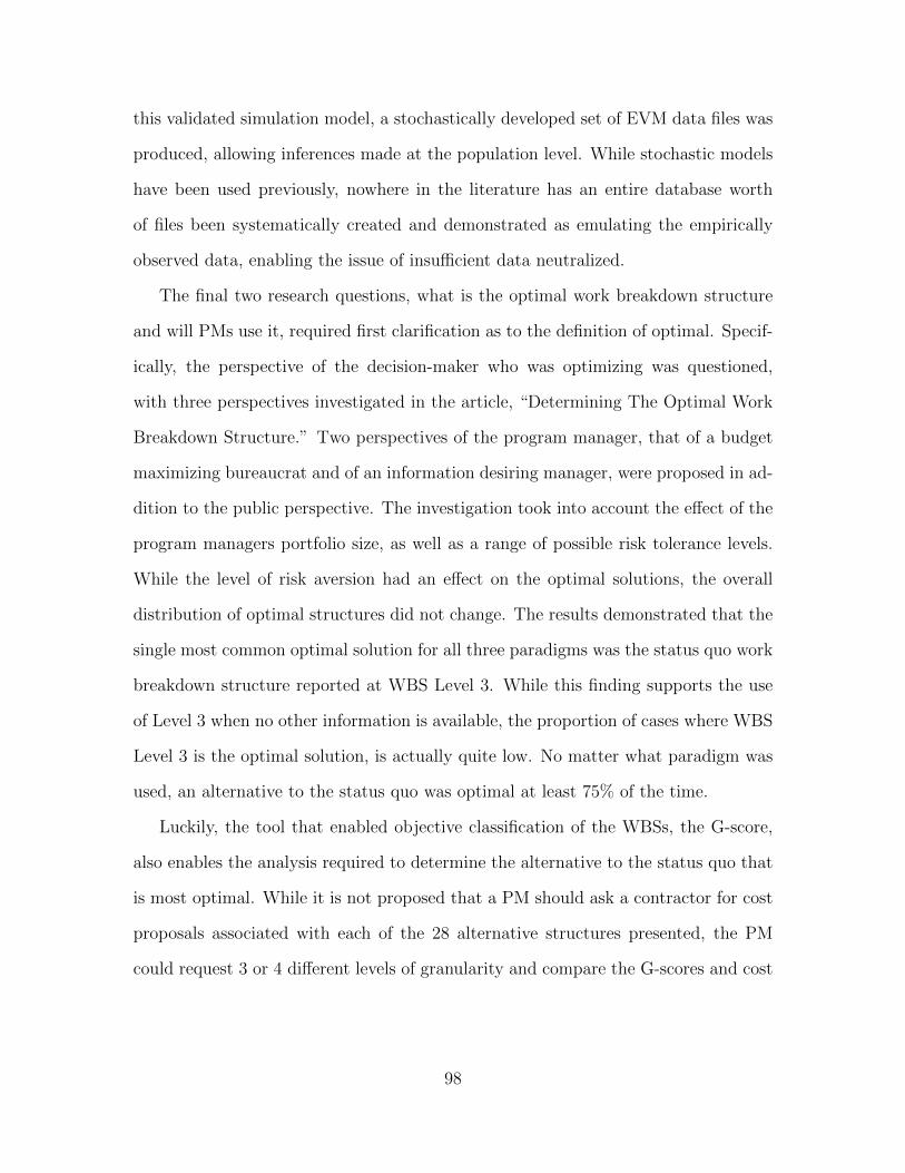
this validated simulation model, a stochastically developed set of EVM data files was

produced, allowing inferences made at the population level. While stochastic models

have been used previously, nowhere in the literature has an entire database worth

of files been systematically created and demonstrated as emulating the empirically

observed data, enabling the issue of insufficient data neutralized.

The final two research questions, what is the optimal work breakdown structure

and will PMs use it, required first clarification as to the definition of optimal. Specif-

ically, the perspective of the decision-maker who was optimizing was questioned,

with three perspectives investigated in the article, “Determining The Optimal Work

Breakdown Structure.” Two perspectives of the program manager, that of a budget

maximizing bureaucrat and of an information desiring manager, were proposed in ad-

dition to the public perspective. The investigation took into account the effect of the

program managers portfolio size, as well as a range of possible risk tolerance levels.

While the level of risk aversion had an effect on the optimal solutions, the overall

distribution of optimal structures did not change. The results demonstrated that the

single most common optimal solution for all three paradigms was the status quo work

breakdown structure reported at WBS Level 3. While this finding supports the use

of Level 3 when no other information is available, the proportion of cases where WBS

Level 3 is the optimal solution, is actually quite low. No matter what paradigm was

used, an alternative to the status quo was optimal at least 75% of the time.

Luckily, the tool that enabled objective classification of the WBSs, the G-score,

also enables the analysis required to determine the alternative to the status quo that

is most optimal. While it is not proposed that a PM should ask a contractor for cost

proposals associated with each of the 28 alternative structures presented, the PM

could request 3 or 4 different levels of granularity and compare the G-scores and cost

98

to implement for each. In this way, an informed decision based on the specific details

of the program and the risk strategy of the PM could be made.

In conclusion, the results demonstrate that there is no silver bullet. There is no

single optimal work breakdown structure for earned value management. The optimal

structure is heavily dependent on the size, scope, and complexity of the contract,

as well as the level of visibility desired by the program manager. Ultimately the

decision and responsibility is still with the PM. What can be said conclusively, no

matter what paradigm, is that there is often something better than the currently

implemented status quo. While the lack of any mechanism for choosing something

other than the status quo has held back program managers, the use of the G-score

now allows appropriate analysis that can aid PMs in making the work breakdown

structure decision deliberately.

99

VII. Appendix: G-Score

Introducing a Metric to Quantify Work Breakdown Structure

Effectiveness

B.J. Fitzpatrick, S.J. Meyer, and J.E. Stubbs

Abstract

The Earned Value Management tool EACG, which uses statistical theory to de-

velop a pessimistic Estimate at Completion for each leaf element in a Government-

Contract Work Breakdown Structure (G-CWBS) was used to construct the G-Score

metric. The purpose of the metric is to quantify the level of oversight granularity

available to program managers based on the G-CWBS structure. A regression model

was constructed using demographic factors, contract information, and the G-Score

metric, that determined the G-Score was a significant predictor of contract price

growth with a P-value of .0002. Additionally, sequential sum of squares analysis was

performed determining the magnitude of additional explanatory power provided by

the inclusion of the G-Score metric in the regression model. While the base model

produced an adjusted R2 of .5062, the sequential R2 of the G-Score metric was .1220,

giving program managers significant insight into expected contract price growth, us-

ing data available before contract award.

100

7.1 Introduction

Program management of publicly funded acquisition programs remains a crucial

focus in the endeavor of public procurement. Defense acquisitions represent a signif-

icant proportion of annual government expenses, providing numerous cases to study,

as well as future opportunities to effect. The focus of this article is to highlight the

cost and schedule control program management tool of Earned Value Management

(EVM), and to introduce a metric that will enable better employment of EVM. A

thorough understanding of the mechanics of EVM will not be required to understand

the metric presented or its usefulness. It is necessary to understand that the Contract

Work Breakdown Structure (CWBS) is a different concept to the contractor and the

government. Each contract which requires Earned Value Management reporting has a

Contractor Contract Work Breakdown Structure(C-CWBS) and a Government Con-

tract Work Breakdown Structure (G-CWBS). While the C-CWBS is broken out to

the work package level that enables the contractor to efficiently manage the resources

that will accomplish work to be delivered, what government program offices receive as

EVM reports is based on the G-CWBS, which is nothing more than a simplification

of the actual data within the C-CWBS.

This study proposes a quantitative metric based on sampling theory that will

provide program managers with a method to calibrate the EVM tools that they

employ, enabling fully informed trade-offs to be made concerning acceptable risk and

costs of reporting.

Previous Research.

In order to test the added benefit of the proposed G-Score metric, a thorough un-

derstanding of programmatic contract growth is desired. Primary data for contract

cost growth comes from the earned value management (EVM) reports that the gov-

101

ernment receives from contractors. In order to calculate the metrics reported, both

a cost and schedule baseline, defined into a series of work packages, is required in

order to compare the contract planned progress against its actual progress. Variances

between the plan and the actual performance are indicative of problems, and provide

an early warning at the project level, and at the leaf element levels broken out.[14]

Previous attempts to forecast cost growth have taken many angles of attack. One

of the first interesting investigations into an early warning signal for programs cen-

tered on CPI stability in government programs. The research conducted by Payne

(1990) and Heise (1991) demonstrated that Cumulative CPI demonstrates stability

past the 20% completion point, giving government program managers an early feel

for the health of their program. While not an explicit estimated cost, this did provide

a vector check very early in the program. Christensen’s work throughout the 1990s

(1992,1993,1994), continued to explore this stability, as well as to find counterexam-

ples of it. One problem with Christensen’s research is that the audience for his work

was not narrow enough. In trying to appeal to both the government and industry,

he confounded his data sources and tried to generalize findings using one data source

to every EVM practitioner, without highlighting the difference between the C-CWBS

and the G-CWBS.

The next great wave of forecasting literature highlights a completely different angle

of attack. Rossetti (2004), White & Sipple (2004), Moore (2005), Bielecki (2005),

McDaniel (2007), and Rusnock (2008) all produced cost growth prediction models

for application in various acquisition types and phases that made use of logistic and

multiple regression. While the individual efforts produced useful insights for their

narrow fields, the small samples sizes due to lack of data hindered the ability to

generalize their research, limiting its impact. One further use of logistic regression

was explored by Trahan (2009) and Thickstun (2010), who were able to predict Over

102

Target Baseline (OTB) contracts, and apply a growth model to forecast the estimate

at completion for those OTB contracts.

Another field of inquiry saw the application of algorithmic data analysis and pre-

dictive analytics to forecast programmatic cost growth. Keaton (2011) tested an al-

gorithm that identified issues in the cost and schedule performance indexes enabling

insight into EAC changes over a 1-12 month horizon, providing a greater amount of

warning to decision makers. Dowling (2012) developed and optimized detection al-

gorithms that were able to alarm decision makers 70% of the time there was a major

programmatic issue. The limitation on Keaton’s research is that only 31 programs

were used, and only WBS Lvl 1 EVM metrics were used. While Dowling’s research

produced an EAC prediction, it was limited to accurately predicting a 4 month hori-

zon only.

Research surrounding the impact of schedule on cost growth, and methods of

increasing the accuracy and usefulness of schedule forecasts has seen greater focus

recently. Crumrine validated that Lipke’s original earned schedule theory proved to

be a more accurate and timely predictor, providing better metrics for Department of

Defense ACAT I programs than the standard Earned Value Management formulations

[5]. In order to refine and better predict program duration issues Lipke, Zwikael,

Henderson, and Anbari (2009) applied statistical methods to WBS Lvl 1 earned value

and earned schedule data. While the use of statistical margin of error estimates was

novel, the assumption that the variance between the 12 programs analyzed represents

the variance within each program is an assumption that is difficult to accept.

While each of these lines of inquiry produced new ways of forecasting contract

cost growth, they each rely on a level of program completion to provide enough data

to produce the analysis. Given the problem illustrated in Figure 3, issues can be

hidden until a very late point of program completion. With this in mind, a tool that

103

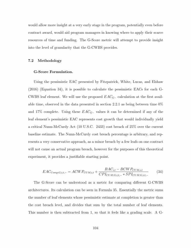
would allow more insight at a very early stage in the program, potentially even before

contract award, would aid program managers in knowing where to apply their scarce

resources of time and funding. The G-Score metric will attempt to provide insight

into the level of granularity that the G-CWBS provides.

7.2 Methodology

G-Score Formulation.

Using the pessimistic EAC presented by Fitzpatrick, White, Lucas, and Elshaw

(2016) (Equation 34), it is possible to calculate the pessimistic EACs for each G-

CWBS leaf element. We will use the proposed EACG− calculation at the first avail-

able time, observed in the data presented in section 2.2.1 as being between time 0%

and 17% complete. Using these EACG− values it can be determined if any of the

leaf element’s pessimistic EAC represents cost growth that would individually yield

a critical Nunn-McCurdy Act (10 U.S.C. 2433) cost breach of 25% over the current

baseline estimate. The Nunn-McCurdy cost breach percentage is arbitrary, and rep-

resents a very conservative approach, as a minor breach by a few leafs on one contract

will not cause an actual program breach, however for the purposes of this theoretical

experiment, it provides a justifiable starting point.

EACComp.G,i,t,− = ACWPCUM,i,t +BACi,t −BCWPCUM,i,t

CPICUM.G,i,t,− ∗ SPICUM.G,i,t,−(34)

The G-Score can be understood as a metric for comparing different G-CWBS

architectures. Its calculation can be seen in Formula 35. Essentially the metric sums

the number of leaf elements whose pessimistic estimate at completion is greater than

the cost breach level, and divides that sum by the total number of leaf elements.

This number is then subtracted from 1, so that it feels like a grading scale. A G-

104

score closer to 1 is desirable as it represents an architecture with enough granularity

that the program manager would be made aware of programmatic issues that would

result in unacceptable cost growth no later than time t. As the EACG metric is

calculated using the weighted standard deviation of the contract leaf elements to

arrive at upper and lower confidence limits, it would be expected that the number

of elements that have an upper estimate that breaks the threshold would go down

as the WBS structure changes towards having more leaf elements that represent an

even distribution of contract funding. If on the other hand, there are only a few leaf

elements that hold most of the contract funding, the weighted standard deviation will

be quite large, leading to many elements that have an upper estimate greater than

the cost breach threshold. As the intent is to give a program manager insight into the

program’s likely contract price growth as close to contract inception as possible, we

will use the first available period of data to calculate the G-Score that will be used

as a potential independent variable.

G = 1−

n∑i=1

EACComp.G,i,t,−BACi

≥ (1 + Cost Breach%) = 1

EACComp.G,i,t,−BACi

< (1 + Cost Breach%) = 0

Total Number of Leaf Elements

(35)

Regression Analysis.

In order to empirically validate the proposed metric, a regression analysis was

accomplished using the calculated percentage increase of contract price in the first

period reported vs the last period reported as the dependent variable. The inde-

pendent variables were chosen by stepwise procedure from the whole effects as well

as polynomial and cross product terms for the variables listed in Tables 16 and 17.

105

A mixed stepwise function was employed in JMPr using P-value threshold criteria

of α = .10 for both entry and exit to selectively refine model elements. All of the

possible independent variables are either demographic in nature, or available from

the contract. By limiting our study to these variables, the utility of the findings

will not be dependent on information that will only become available after a certain

percentage of program completion.

Table 16. Discrete Variables

Variable LevelsLead Branch Army

NavyAir ForceJoint

Contract Phase EMDRDTEProductionOther

System Type Aircraft SystemElectronic SystemMissile SystemOrdinanceSea SystemsSpace SystemSurface VehicleUnmanned Air SystemLaunch VehicleAutomated Information SystemCommon Elements

Contract Type Cost PlusFirm Fixed PriceFixed Price IncentiveOther

ACAT Level ACAT I - 1ACAT I - 2ACAT I - 3ACAT I - 4ACAT I - 5ACAT IIACAT III

106

Table 17. Continuous Variables

Variable UnitsG-CWBS Leaf Elements Leaf ElementLength of Contract MonthsG-Score Nominal 0-1

Data for Regression Analysis.

The data used for analysis was retrieved from the Office of the Secretary of De-

fense’s Cost Assessment Data Enterprise (OSD CADE) system. Of the 276 contract

files available in the database, 108 had EVM data broken out into WBS elements, of

which 70 contracts had data representing over 60% contract completion (Fitzpatrick

et. al., 2016). Once these contracts were used in a preliminary regression model, 3

were shown to be heavily influential as shown in Table 18.

Contract MPS 0.7659 -0.3768 0.4841 0.5624 0.093 -0.1609 -0.0568 0.1595 0.0724

GCSS-Army 1.5551 0.2038 0.1427 -0.4994 -0.2455 1.401 0.1432 -0.4663 0.32DDG1000 0.9838 -0.0694 0.6028 -0.1866 -0.2531 0.0235 -0.0362 -0.1652 0.1197

◦ ◦ ◦ ◦ ◦ ◦ ◦ ◦ ◦ ◦ ◦ ◦ ◦DFFITSDFBETA - InterceptDFBETA - Contract LengthDFBETA - ACAT 3/4DFBETA - ACAT 1-1DFBETA - Automated Information SystemsDFBETA - Number of Leaf ElementsDFBETA - G-ScoreCook’s Distance

DFFITS threshold calculated at 2√

p/n DFBETA threshold calculated at 2√n

Table 18. Influential Data Point Diagnostics

The raw CADE data files were examined, and these three programs each demon-

strated similar behavior of the dependent variable, the Contract Price Element, indi-

cating that what was reported was likely the contract burn rate at each period, and

not the actual total contract price at each period. Given this reporting discrepancy,

these contracts were not able to be used in the final analysis, as they did not provide

1While generally broken out into only ACAT I, II, III, or IV, this analysis divided ACAT I intofive levels based on funding.

107

the contract price baseline at period 0 enabling comparison with contact price in the

last period reported. Final program contracts used for analysis are listed in Tables 2,

3, 4, and 5, and demographic information is illustrated in Figures 4, 5, 6, and 7.

Final Regression Model.

With the three cases eliminated from our data set, the modeling process was iter-

ated again and resulted in the final regression model shown in Equation 36, with the

resulting model having an adjusted R2 = .5062. The model satisfied all assumptions

as the programs were independent, constant variance was verified by plotting the

predicted values by the residual values, and normality of the residuals was verified by

the Shapiro-Wilkes test resulting with a P-value of 0.0687.

Y = −0.25722 + 0.0047864(Months) + 0.1452155(ACAT.3)+

0.2605086(ACAT.1 1) + 0.1848117(Automated.InformationSystems)+

0.000072682(Number.of.Leaf.Elements) + 0.310968(G− ScoreF irst) (36)

G-Score Value Validation.

Using the regression model, the G-Score parameter’s P-value will be observed to

determine if it indeed contributes significantly to predict contract cost growth. The

sequential sum of squares value of the G-Score as the final parameter will also be

calculated to determine the Partial R2 of the G-Score parameter in order to illustrate

the additional power that is gives the model. Finally, a bootstrap analysis using 1000

iterations will be performed to show the range of the G-Score parameter Sequential

R2 expected.

108

7.3 Results

Regression Model Results.

Based on the regression model in Equation 36, the resulting parameters, along

with their standard errors, P-values, and variance inflation factors are illustrated in

Figure 19. All listed parameters are significant at the desired α = .05 level, and all of

the VIF scores assure that there is not multicollinearity of the parameters present.

Table 19. Final Model Parameter Output

Term β Estimate Std Error P-Val VIFIntercept -0.25722 0.064681 0.0002 .Months 0.0047864 0.000695 < .0001 1.3764ACAT3 0.1452155 0.046132 0.0026 1.6843ACAT1-1 0.2605086 0.058546 < .0001 1.2643Automated Information Systems 0.1848117 0.080346 0.0249 1.1495Number of Leaf Elements 0.000072682 0.000033 0.0313 1.0447G-Score First 0.310968 0.076993 0.0002 1.2068

Partial R2 Bootstrap Analysis Result.

The results from the sequential sum of squares for the final model is shown in

Table 20. Even after the five previous parameters are taken into account, the G-

Score at the first available time period explains 12.2% of the variability in the model.

Given that the entire model explained 50.62% of contract price growth variability, this

represents a substantial increase in explanatory power due to the introduction of the

G-Score metric. The Partial R2 Bootstrap Analysis produced the results illustrated

in Figure 46. The mean Partial R2 = .1173 is very similar to the model Partial

R2 = .1220, demonstrating the robust explanatory power of the G-Score metric. The

close observer will also notice a small bimodal bump where Partial R2 ≈ .5. After

reviewing the bootstrap data log, it was found that these random samples did not

contain any Automated Information System data points, dropping that parameter

109

Table 20. Sequential Sum of Squares Analysis

Term Sequential Sum of Squares Partial R2

Months 0.61901 0.2192ACAT3 0.01706 0.0060ACAT1-1 0.30704 0.1087Automated Information Systems 0.20809 0.0737Number of Leaf Elements 0.06029 0.0214G-Score First 0.34457 0.1220

from the model, where the G-Score metric became far more significant, essentially

picking up the explanatory slack.

Figure 46. Bootstrap Analysis of G-Score Impact on Total R2

7.4 Discussion and Conclusion

The G-Score metric has been demonstrated to be a significant predictor variable

in modeling contract price growth between the first reported contract price and the

final reported contract price. Furthermore, by adding the parameter to the model, an

110

additional 12% of variability is able to be explained that would not have been with it.

While reviewing the literature, there have been models that surpass the explanatory

power of the model presented here, however they have all required inputs far greater

than simple demographic and contract factors. This increase in insight could greatly

help program managers responsible for stewardship of public funds.

While this significant increase in explanatory power can help program managers

in their task, it should be highlighted that a high G-Score will not ensure low cost

growth. A better interpretation would be that a high G-Score may be indicative of

a well defined and well understood program, whereas a low g-score may represent an

undefined program, which when better understood will simply cost more. Another

interpretation is that a high G-Score will represent a G-CWBS that provides enough

granularity to the PM, that when an issue arises, the PM becomes aware of it imme-

diately, instead of being subjected to the potential lag illustrated in Figure 3. With

this in mind, if during contract negotiations, the contractor proposes a G-CWBS

with a low G-Score, the PM may wish to request a more detailed breakout in the

leaf elements that are causing the low metric. If the contractor provides the detailed

breakout, the PM will have the visibility necessary throughout the contract period,

whereas if the contractor is unable to give a more defined breakout, the leaf elements

in question may not be as developed as previously hoped, and additional mitigation

efforts may be needed to address the programmatic risk.

111

Bibliography

1. Bielecki, M. J. V., & White, E. D. (2005). Estimating cost growth from schedule

changes: A regression. Cost engineering, 47(8), 28-34.

2. Christensen, D. S., Antolini, R. C., & McKinney, J. W. (1992). A review of estimate

at completion research. In Cost estimating and analysis (pp. 207-224). Springer

New York.

3. Christensen, D. S. (1993). The estimate at complete problem: a review of three

studies. International Journal of Project Management, 24(1), 37-42.

4. Christensen, D. S. (1994). Using performance indices to evaluate the estimate at

completion. The Journal of Cost Analysis, 11(1), 17-23.

5. Crumrine, K. T. (2013). A Comparison of Earned Value Management and Earned

Schedule as Schedule Predictors on DoD ACAT I Programs (No. AFIT-ENV-13-

M-36). Air Force Institute of Technology Wright-Patterson AFB OH Graduate

School of Engineering and Management.

6. Dowling, A. W. (2012). Using Predictive Analytics to Detect Major Problems

in Department of Defense Acquisition Programs (No. AFIT/GCA/ENC/12-03).

Air Force Institute of Technology Wright-Patterson AFB OH Graduate School of

Engineering and Management.

7. Fitzpatrick, B., White, E., Lucas, B., & Elshaw, J. (2016). Alternative Formulation

of a Pessimistic Estimate at Completion. Journal of Cost Analysis and Parametrics,

Submitted, pending acceptance.

112

8. Heise, S. R. (1991). A review of cost performance index stability (No.

AFIT/GSM/LSY-91S-12). Air Force Institute of Technology Wright-Patterson

AFB OH Graduate School of Systems and Logistics.

9. Keaton, C. G., White, E. D., & Unger, E. J. (2011). Using earned value data to

detect potential problems in acquisition contracts. Journal of Cost Analysis and

Parametrics, 4(2), 148-159.

10. Lipke, W., Zwikael, O., Henderson, K., and Anbari, F. (2009). Prediction of

Project Outcome: The Application of Statistical Methods to Earned Value Man-

agement and Earned Schedule Performance Indexes. International Journal of

Project Management, 27(4), 400-407.

11. McDaniel, C. J., & White III, E. D. (2007). Predicting engineering and schedule

procurement cost growth for major DoD programs. Journal of Public Procurement,

7(3), 362.

12. Moore, G. W., & White III, E. D. (2005). A regression approach for estimating

procurement cost. Journal of Public Procurement, 5(2), 187.

13. Payne, K. (1990). An investigation of the stability of the cost performance index

(No. AFIT/GCA/LSY/90S-6). Air Force Institute of Technology Wright-Patterson

AFB OH Graduate School of Engineering and Management.



15. Rossetti, M. B., & White III, E. T. D. (2004). A two-pronged approach to estimate

procurement cost growth in major DoD weapon systems. The Journal of Cost

Analysis & Management, 6(2), 11-21.

113

16. Rusnock, C. F. (2008). Predicting Cost and Schedule Growth for Military and

Civil Space Systems (No. AFIT/GRD/ENC/08M-01). Air Force Institute of Tech-

nology Wright-Patterson AFB OH Graduate School of Engineering and Manage-

ment.

17. Thickstun, K. E. (2010). Predicting Over Target Baseline (OTB) Acquisition Con-

tracts (No. AFIT/GCA/ENC/10-01). Air Force Institute of Technology Wright-

Patterson AFB OH Graduate School of Engineering and Management.

18. Trahan, E. N. (2009). An evaluation of growth models as predictive tools for

estimates at completion (EAC) (No. AFIT/GFA/ENC/09-01). Air Force Institute

of Technology Wright-Patterson AFB OH Graduate School of Engineering and

Management.

19. White III, E. D., Sipple, V. P., & Greiner, M. A. (2004). Using logistic and

multiple regression to estimate engineering cost risk. The Journal of Cost Analysis

& Management, 6(1), 67-79.

114

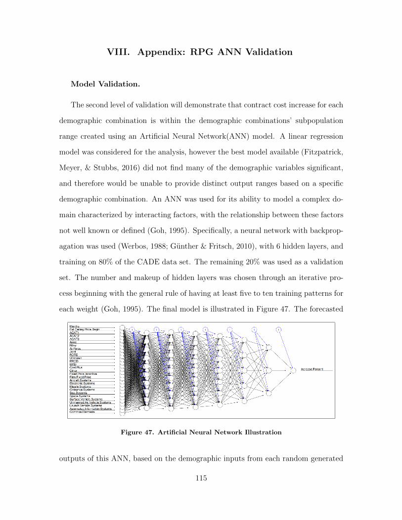
VIII. Appendix: RPG ANN Validation

Model Validation.

The second level of validation will demonstrate that contract cost increase for each

demographic combination is within the demographic combinations’ subpopulation

range created using an Artificial Neural Network(ANN) model. A linear regression

model was considered for the analysis, however the best model available (Fitzpatrick,

Meyer, & Stubbs, 2016) did not find many of the demographic variables significant,

and therefore would be unable to provide distinct output ranges based on a specific

demographic combination. An ANN was used for its ability to model a complex do-

main characterized by interacting factors, with the relationship between these factors

not well known or defined (Goh, 1995). Specifically, a neural network with backprop-

agation was used (Werbos, 1988; Gunther & Fritsch, 2010), with 6 hidden layers, and

training on 80% of the CADE data set. The remaining 20% was used as a validation

set. The number and makeup of hidden layers was chosen through an iterative pro-

cess beginning with the general rule of having at least five to ten training patterns for

each weight (Goh, 1995). The final model is illustrated in Figure 47. The forecasted

Figure 47. Artificial Neural Network Illustration

outputs of this ANN, based on the demographic inputs from each random generated

115

program, were used as the comparative data set for another validation t-test. As this

method of validation is experimental, the t-test was conducted at both α = 0.05 and

α = 0.01.

8.1 Results

Figure 48 illustrates the distribution of t-test results at the demographic combina-

tion level. A perfectly passing model would be one in which the randomly generated

program data and corresponding ANN forecasts for all demographic combinations

were shown to not be significantly different. At α = 0.05 only 66% of the demo-

graphic combinations pass this stage of validation. With a relaxed α = 0.01, the

pass rate increases to 84%, however this still leaves a large number of demographic

combinations failing validation. An investigation into the characteristics of the com-

binations that failed began by highlighting the combinations that appeared in the

CADE data set. Figure 49 illustrates only those 44 combinations, which mirror the

distribution of passing and failing combinations of the population. The percent of

CADE combinations that pass is almost identical at the α = 0.05 level, and is sim-

ilarly close at the α = 0.01 level. Figure 50 shows the same distribution of CADE

combinations, with the additional dimension of weighting. As previously stated, of

the 44 demographic combinations represented in the CADE data set, the most nu-

merous had 5 replications, with most being unique. This graphic indicates that those

combinations with multiple replicates had a proclivity to fail.

8.2 Discussion

The demographic combination validation did not provide conclusive results. Par-

ticularly, the tendency of the most numerous demographic combinations to fail, raises

concern. This could be indicative of model overfit, causing the forecasted data set

116

Figure 48. Predicted vs Generated Increase Ranges Per Demographic Combination

from the ANN to have a much smaller variance than the random generated data set.

Alternatively, the reason for this validation failure could be due to inaccuracy in the

random program generator, or some combination of both the ANN and the RPG. A

simultaneous calibration procedure and more ANN structures and training profiles

will be implemented in the future in an effort to be able to make the specific infer-

ences that would become possible with validated demographic combination results.

As it stands, the results presented here are limited in their applicability to generalized

statements made at the validated population level.

A great limitation of the results of the simulation model, is that the individual

demographic combinations did not pass validation. While greater than half of the

demographic combinations did pass, the fact that they all did not pass raised enough

uncertainty as to make the use for inference of the demographic combinations unde-

fended. The reason for this failure of validation could lie with the random program

117

Figure 49. Demographic Combinations Represented in CADE Data Set

generator simulation model or with the artificial neural network forecast that was

used to validate the demographic combinations. As both of these processes were

highly complex, is not known which one or both and in which what proportion blame

lies. Without further research, only general statements can come from the simula-

tion. Specific statements are not fully supported due to the lack of demographic

combinations validation.

8.3 Appendix

Concerning the demographic combinations that failed validation, the following

investigative graphs provide some insight into characteristics and trends. While the

figures depict the results of all demographic combinations(DC), the specific combi-

nations that were represented in the CADE data set have been extracted into tables

for review. Further analysis into the shared characteristics, if any, of the DCs that

118

Figure 50. CADE Demographic Combinations by Number of Occurrences

failed may provide insight for future modifications to the simulation model or choice

of validation protocols.

119

Table 21. CADE Combination Groups by Branch

Army Count Pass Navy Count Pass Air Force Count Pass Joint Count Pass

1-2-A-1 2 1 2-2-E-1 2 0 3-1-A-1 5 0 4-3-L-1 2 1

1-3-D-1 1 1 2-2-C-3 1 1 3-1-F-1 1 0 4-2-K-1 1 0

1-2-B-1 4 0 2-2-C-1 2 1 3-2-B-1 5 0 4-1-D-3 1 1

1-1-G-2 1 1 2-2-B-2 1 0 3-2-D-1 1 1

1-2-C-2 1 1 2-2-A-1 2 0 3-1-D-1 1 1

1-2-G-3 1 1 2-2-B-1 5 0 3-1-A-3 1 1

1-1-B-1 1 1 2-3-E-3 1 1 3-3-J-1 1 1

1-1-B-3 1 1 2-1-A-3 1 1 3-3-A-1 1 0

1-1-L-1 2 1 2-2-A-3 1 1 3-2-A-1 1 1

1-1-A-1 1 1 2-2-E-2 1 1 3-2-B-3 1 0

1-1-C-1 1 0 2-3-E-2 2 1 3-2-F-3 1 0

1-1-C-3 1 1 2-2-F-1 1 0 3-1-C-2 1 1

1-2-G-1 1 1 2-1-E-1 1 0 3-3-H-1 2 1

3-1-F-3 1 1

3-1-D-2 1 1

Total 18 Total 21 Total 24 Total 4

120

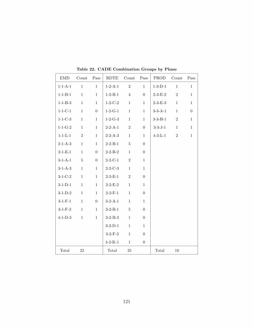
Table 22. CADE Combination Groups by Phase

EMD Count Pass RDTE Count Pass PROD Count Pass

1-1-A-1 1 1 1-2-A-1 2 1 1-3-D-1 1 1

1-1-B-1 1 1 1-2-B-1 4 0 2-3-E-2 2 1

1-1-B-3 1 1 1-2-C-2 1 1 2-3-E-3 1 1

1-1-C-1 1 0 1-2-G-1 1 1 3-3-A-1 1 0

1-1-C-3 1 1 1-2-G-3 1 1 3-3-H-1 2 1

1-1-G-2 1 1 2-2-A-1 2 0 3-3-J-1 1 1

1-1-L-1 2 1 2-2-A-3 1 1 4-3-L-1 2 1

2-1-A-3 1 1 2-2-B-1 5 0

2-1-E-1 1 0 2-2-B-2 1 0

3-1-A-1 5 0 2-2-C-1 2 1

3-1-A-3 1 1 2-2-C-3 1 1

3-1-C-2 1 1 2-2-E-1 2 0

3-1-D-1 1 1 2-2-E-2 1 1

3-1-D-2 1 1 2-2-F-1 1 0

3-1-F-1 1 0 3-2-A-1 1 1

3-1-F-3 1 1 3-2-B-1 5 0

4-1-D-3 1 1 3-2-B-3 1 0

3-2-D-1 1 1

3-2-F-3 1 0

4-2-K-1 1 0

Total 22 Total 35 Total 10

121

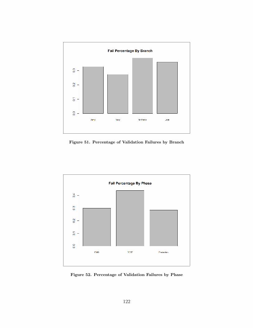
Figure 51. Percentage of Validation Failures by Branch

Figure 52. Percentage of Validation Failures by Phase

122

Table 23. CADE Combination Groups by Contract

Cost Plus Count Pass Firm Fixed Price Count Pass Fixed Price Incentive Count Pass

1-1-A-1 1 1 1-1-G-2 1 1 1-1-B-3 1 1

1-1-B-1 1 1 1-2-C-2 1 1 1-1-C-3 1 1

1-1-C-1 1 0 2-2-B-2 1 0 1-2-G-3 1 1

1-1-L-1 2 1 2-2-E-2 1 1 2-1-A-3 1 1

1-2-A-1 2 1 2-3-E-2 2 1 2-2-A-3 1 1

1-2-B-1 4 0 3-1-C-2 1 1 2-2-C-3 1 1

1-2-G-1 1 1 3-1-D-2 1 1 2-3-E-3 1 1

1-3-D-1 1 1 3-1-A-3 1 1

2-1-E-1 1 0 3-1-F-3 1 1

2-2-A-1 2 0 3-2-B-3 1 0

2-2-B-1 5 0 3-2-F-3 1 0

2-2-C-1 2 1 4-1-D-3 1 1

2-2-E-1 2 0

2-2-F-1 1 0

3-1-A-1 5 0

3-1-D-1 1 1

3-1-F-1 1 0

3-2-A-1 1 1

3-2-B-1 5 0

3-2-D-1 1 1

3-3-A-1 1 0

3-3-H-1 2 1

3-3-J-1 1 1

4-2-K-1 1 0

4-3-L-1 2 1

Total 47 Total 8 Total 12

123

Figure 53. Percentage of Validation Failures by Contract Type

Figure 54. Percentage of Validation Failures by System Type

124

Table 24. CADE Combination Groups by System

Aircraft Count Pass Electronics Count Pass Missiles Count Pass Ordinance Count Pass

3-1-A-1 5 0 3-2-B-1 5 0 3-1-C-2 1 1 3-2-D-1 1 1

3-1-A-3 1 1 3-2-B-3 1 0 1-2-C-2 1 1 3-1-D-1 1 1

3-3-A-1 1 0 1-2-B-1 4 0 1-1-C-1 1 0 3-1-D-2 1 1

3-2-A-1 1 1 1-1-B-1 1 1 1-1-C-3 1 1 1-3-D-1 1 1

1-2-A-1 2 1 1-1-B-3 1 1 2-2-C-3 1 1 4-1-D-3 1 1

1-1-A-1 1 1 2-2-B-2 1 0 2-2-C-1 2 1

2-2-A-1 2 0 2-2-B-1 5 0

2-1-A-3 1 1

2-2-A-3 1 1


Sea Count Pass Space Count Pass Surf Veh Count Pass Unmn Air Count Pass

2-2-E-1 2 0 3-1-F-1 1 0 1-1-G-2 1 1 3-3-H-1 2 1

2-3-E-3 1 1 3-2-F-3 1 0 1-2-G-3 1 1

2-2-E-2 1 1 3-1-F-3 1 1 1-2-G-1 1 1

2-3-E-2 2 1 2-2-F-1 1 0

2-1-E-1 1 0


Unmn Sea Count Pass Launch Count Pass AIS Count Pass Common Count Pass

3-3-J-1 1 1 4-2-K-1 1 0 1-1-L-1 2 1

4-3-L-1 2 1


125

REPORT DOCUMENTATION PAGE Form ApprovedOMB No. 0704–0188

The public reporting burden for this collection of information is estimated to average 1 hour per response, including the time for reviewing instructions, searching existing data sources, gathering andmaintaining the data needed, and completing and reviewing the collection of information. Send comments regarding this burden estimate or any other aspect of this collection of information, includingsuggestions for reducing this burden to Department of Defense, Washington Headquarters Services, Directorate for Information Operations and Reports (0704–0188), 1215 Jefferson Davis Highway,Suite 1204, Arlington, VA 22202–4302. Respondents should be aware that notwithstanding any other provision of law, no person shall be subject to any penalty for failing to comply with a collectionof information if it does not display a currently valid OMB control number. PLEASE DO NOT RETURN YOUR FORM TO THE ABOVE ADDRESS.

1. REPORT DATE (DD–MM–YYYY) 2. REPORT TYPE 3. DATES COVERED (From — To)

4. TITLE AND SUBTITLE 5a. CONTRACT NUMBER

5b. GRANT NUMBER

5c. PROGRAM ELEMENT NUMBER

5d. PROJECT NUMBER

5e. TASK NUMBER

5f. WORK UNIT NUMBER

6. AUTHOR(S)

7. PERFORMING ORGANIZATION NAME(S) AND ADDRESS(ES) 8. PERFORMING ORGANIZATION REPORTNUMBER

9. SPONSORING / MONITORING AGENCY NAME(S) AND ADDRESS(ES) 10. SPONSOR/MONITOR’S ACRONYM(S)

11. SPONSOR/MONITOR’S REPORTNUMBER(S)

12. DISTRIBUTION / AVAILABILITY STATEMENT

13. SUPPLEMENTARY NOTES

14. ABSTRACT

15. SUBJECT TERMS

16. SECURITY CLASSIFICATION OF:

a. REPORT b. ABSTRACT c. THIS PAGE

17. LIMITATION OFABSTRACT

18. NUMBEROFPAGES

19a. NAME OF RESPONSIBLE PERSON

19b. TELEPHONE NUMBER (include area code)

Standard Form 298 (Rev. 8–98)Prescribed by ANSI Std. Z39.18

24–03–2016 Master’s Thesis Sept 2014 — Mar 2016

DETERMINING THE OPTIMAL WORK BREAKDOWNSTRUCTURE FOR GOVERNMENT ACQUISITION CONTRACTS

Brian J. Fitzpatrick, Captain, USAF

Air Force Institute of TechnologyGraduate School of Engineering and Management (AFIT/EN)2950 Hobson WayWPAFB OH 45433-7765


Left Intentionally Blank

DISTRIBUTION STATEMENT A:APPROVED FOR PUBLIC RELEASE; DISTRIBUTION UNLIMITED.

The optimal level of Government Contract Work Breakdown Structure (G-CWBS) reporting for the purposes of EarnedValue Management was inspected. The G-Score Metric was proposed, which can quantitatively grade a G-CWBS, basedon a new method of calculating an Estimate At Completion (EAC) cost for each reported element. A random programgenerator created in R replicated the characteristics of DOD program artifacts retrieved from the Cost Analysis DataEnterprise (CADE) system. The generated artifacts were validated as a population, however validation at thedemographic combination level using an artificial neural network was inconclusive. Comparative WBS forms were createdfor a sample of the generated programs, and used to populate a decision tree. Utility theory tools were applied usingthree utility perspectives, and optimal WBSs were identified. Results demonstrated that reporting at WBS level 3 is themost common optimal structure, however 75% of the time a different optimal structure exists.

EVM, G-Score, R, Simulation, EAC, Utility, WBS

U U U U 141

Edward D. White, AFIT/ENC

937-255-3636 ext. 4540; [email protected]

AIR FORCE INSTITUTE OF TECHNOLOGY · Air Force Institute of Technology ... Technology Readiness...

Documents

Transcript of AIR FORCE INSTITUTE OF TECHNOLOGY · Air Force Institute of Technology ... Technology Readiness...