AIR FORCE INSTITUTE OF TECHNOLOGY · DEPARTMENT OF THE AIR FORCE AIR UNIVERSITY ... The Inertial...
232
PERFORMANCE TRADEOFF STUDY OF A GPS-AIDED INS FOR A ROCKET TRAJECTORY THESIS Muhittin Istanbulluoglu, 1st Lt, TuAF AFIT/GE/ENG/02M-11 DEPARTMENT OF THE AIR FORCE AIR UNIVERSITY AIR FORCE INSTITUTE OF TECHNOLOGY Wright-Patterson Air Force Base, Ohio APPROVED FOR PUBLIC RELEASE; DISTRIBUTION UNLIMITED.
Transcript of AIR FORCE INSTITUTE OF TECHNOLOGY · DEPARTMENT OF THE AIR FORCE AIR UNIVERSITY ... The Inertial...

PERFORMANCE TRADEOFF STUDY OF A GPS-AIDED INS FOR A ROCKET
TRAJECTORY
THESIS
Muhittin Istanbulluoglu, 1st Lt, TuAF
AFIT/GE/ENG/02M-11
DEPARTMENT OF THE AIR FORCE AIR UNIVERSITY
AIR FORCE INSTITUTE OF TECHNOLOGY
Wright-Patterson Air Force Base, Ohio
APPROVED FOR PUBLIC RELEASE; DISTRIBUTION UNLIMITED.

The views expressed in this thesis are those of the author and do not reflect the official policy or position of the United States Air Force, Department of Defense, or the U. S. Government.

AFIT/GE/ENG/02M-11
PERFORMANCE TRADEOFF STUDY OF A GPS-AIDED INS FOR A ROCKET TRAJECTORY
THESIS
Presented to the Faculty
Department of Systems and Engineering Management
Graduate School of Engineering and Management
Air Force Institute of Technology
Air University
Air Education and Training Command
In Partial Fulfillment of the Requirements for the
Degree of Master of Science in Engineering and Environmental Management
Muhittin Istanbulluoglu, BS
1st Lt, TuAF
March 2002
APPROVED FOR PUBLIC RELEASE; DISTRIBUTION UNLIMITED.
ii

Acknowledgments
I would like to thank my thesis advisor, Dr. Peter Maybeck, for his support,
patience and guidance through this research. I feel myself lucky for being his thesis
student. I would also like to thank my thesis committee members Lt. Col. Mikel M.
Miller and Maj. John F. Raquet, for their help and support. Special thanks to Dr. Stanton
Musick for his help and support in my studies.
I also would like to thank the great Turkish nation and Turkish Air Force for
providing me such a quality Master’s Program opportunity. I believe, I have done my
best to take full advantage of the experience that I have gotten in this program to serve
my country better.
I will not forget to thank my wife for her extreme patience and support, and my
parents and all my family members for the values they thought me, which helped me a lot
to complete this program.
iv
Table of Contents
Page
Acknowledgments............................................................................................................. iv
Table of Contents ................................................................................................................ v
List of Figures ..................................................................................................................... x
List of Tables.................................................................................................................... xiv
AFIT/GE/ENG/02M-11
Abstract ............................................................................................................................ xvi
I Introduction.......................................................................................................... I-1
1.1 Background .............................................................................................. I-2
1.2 Key Terms ................................................................................................ I-7
1.3 Literature Review..................................................................................... I-8
1.3.1 Benefits of Integrated Systems..................................................... I-8
1.3.2 INS/GPS Integration Techniques ............................................... I-10
1.3.3 Integration Kalman Filter Error and Measurement Models ....... I-11
1.3.4 The Chosen Launch Vehicle (Atlas IIAS) for Simulations........ I-12
1.4 Problem Statement ................................................................................. I-14
1.5 Assumptions ........................................................................................... I-17
1.6 Scope ..................................................................................................... I-22
1.7 Summary ................................................................................................ I-24
II Theory................................................................................................................. II-1
2.1 Introduction ............................................................................................. II-1
v
2.2 Ring Laser Gyro (RLG) Strapdown INS................................................. II-1
2.3 Barometric Altimeter............................................................................... II-3
2.4 Global Positioning System (GPS) ........................................................... II-4
2.4.1 GPS Space Segment .................................................................... II-5
2.4.2 GPS Control Segment ................................................................. II-6
2.4.3 GPS User Segment ...................................................................... II-7
2.5 Differential GPS (DGPS) ....................................................................... II-8
2.6 Reference Frames.................................................................................... II-9
2.6.1 Inertial Frame ( x i , y i , z i ) ...................................................... II-11
2.6.2 Earth Frame ( x e , y e , z e ) ....................................................... II-12
2.6.3 Geographic Frame ( x g , y g , z g ) = (E, N, U).......................... II-13
2.6.4 Navigation Frame ( x n , y n , z n ).............................................. II-14
2.6.5 Body Frame ( x b , y b , z b )........................................................ II-15
2.7 Reference Frames Transformations ...................................................... II-16
2.7.1 Inertial Frame to Earth Frame, C ........................................... II-17 ei
2.7.2 Earth Frame to Geographic Frame, C ................................... II-17 ge
2.7.3 Earth Frame to Navigation Frame, .................................... II-17 neC
2.7.4 Geographic Frame to Navigation Frame, ............................ II-18 ngC
2.7.5 Geographic Frame to Body Frame, C .................................... II-18 bg
2.7.6 Navigation Frame to Body Frame, ..................................... II-19 bnC
vi
2.8 Kalman Filter Theory ............................................................................ II-19
2.8.1 What is a Kalman Filter?........................................................... II-19
2.8.2 Kalman Filter Example ............................................................. II-20
2.8.3 Linear Kalman Filter ................................................................. II-26
2.8.4 Linearized and Extended Kalman Filter.................................... II-30
2.9 Summary ............................................................................................... II-34
III Design Methodology and Error Models................................................................III-1
3.1 Overview ................................................................................................III-1
3.2 Introduction to MatSOFE.......................................................................III-1
3.3 Introduction to PROFGEN.....................................................................III-6
3.4 Satellite Vehicle Data Using WSEM 3.6 .............................................III-11
3.5 The SNSM Computer Model ...............................................................III-13
3.6 Space Navigation System Model (SNSM) Description .......................III-16
3.6.1. The Inertial Navigation System (INS) Model ..........................III-18
3.6.1.1 The 93-State LN-93 Error Model.......................................III-19
3.6.1.2 The 39-State INS Truth Model...........................................III-20
3.6.1.3 The 11-State INS Filter Model...........................................III-21
3.6.2. The Global Positioning System (GPS) Model .........................III-22
3.6.2.1 The 30-State GPS Truth Model..........................................III-23
3.6.2.2 The 22-State DGPS Truth Model.......................................III-26
3.6.2.3 The 2-State GPS/DGPS Filter Model.................................III-28
3.6.2.4 GPS Measurement Model ..................................................III-29
3.6.2.5 DGPS Measurement Model ...............................................III-32
vii
3.7 Chapter Summary.................................................................................III-34
IV Results and Analysis ..........................................................................................IV-1
4.1 Validation of MATSOFE ......................................................................IV-2
4.1.1. Comparison to Gray’s Results [10]............................................IV-4
4.1.2. Comparison to Britton’s Results [6]...........................................IV-6
4.2 The Launch Vehicle (Atlas IIAS) Flight Profile ...................................IV-7
4.3 Development of the Three Types of INS’s ............................................IV-9
4.4 Filter Tuning Process ...........................................................................IV-10
4.5 Performance Analysis ..........................................................................IV-12
4.5.1. Baro-Altimeter and Standard GPS Aiding Cases.....................IV-12
4.5.1.1 Case I, 0.4 nm/hr CEP INS/Baro-Alt./ Std.GPS ................IV-12
4.5.1.2 Case III, 2.0 nm/hr CEP INS/ Baro-Alt/ Std.GPS..............IV-14
4.5.1.3 Case V, 4.0 nm/hr CEP INS/ Baro-Alt/ Std.GPS...............IV-15
4.5.2. Baro-Altimeter and P-Code DGPS Aiding Cases ....................IV-15
4.5.2.1 Case II, 0.4 nm/hr CEP INS/Baro-Alt./P-Code DGPS ......IV-16
4.5.2.2 Case IV, 2.0 nm/hr CEP INS/Baro-Alt./P-Code DGPS.....IV-17
4.5.2.3 Case VI, 4.0 nm/hr CEP INS/Baro-Alt./P-Code DGPS.....IV-18
4.6 Chapter Summary.................................................................................IV-19
V. Conclusions and Recommendations....................................................................V-1
5.1 Conclusion................................................................................................V-1
5.2 Recommendations ....................................................................................V-3
Appendix A Error State Definitions for the SNSM Truth and Filter Models..............A-1
Appendix B Dynamics Matrices and Noise Values .................................................... B-1
viii
Appendix C PROF_IN Input File ................................................................................ C-1
Appendix D Atlas IIAS Rocket Profile Plots ..............................................................D-1
Appendix E True Ephemeris Generation Process ....................................................... E-1
Appendix F Plots Obtained from WSEM 3.6 ..............................................................F-1
Appendix G MatSOFE Validation Plots......................................................................G-1
Appendix H Tuning Examples.....................................................................................H-1
Appendix I Plots of Case I .......................................................................................... I-1
Appendix J Plots of Case II ......................................................................................... J-1
Appendix K Plots of Case III.......................................................................................K-1
Appendix L Plots of Case IV....................................................................................... L-1
Appendix M. Plots of Case V....................................................................................... M-1
Appendix N Plots of Case VI.......................................................................................N-1
ix
List of Figures
Page
Figure I-1. Loosely coupled INS/GPS integration .......................................................... I-4
Figure I-2. Tightly coupled INS/GPS integration ........................................................... I-4
Figure I-3. The Principle of Satellite Navigation [25] .................................................... I-5
Figure I-4. Earth’s Orbits [26]....................................................................................... I-13
Figure I-5. Atlas IIAS.................................................................................................... I-13
Figure I-6. Space Navigation System Model (SNSM) Simulation ............................... I-21
Figure II-1. GPS Major Segments.................................................................................. II-4
Figure II-2. GPS Orbital Planes ..................................................................................... II-6
Figure II-3. GPS master control & monitor stations ...................................................... II-7
Figure II-4. Circle Diagram Relating PROFGEN Frames [29] ................................... II-10
Figure II-5. Inertial Frame............................................................................................ II-11
Figure II-6. Earth Frame............................................................................................... II-12
Figure II-7. Geographic Frame..................................................................................... II-13
Figure II-8. Navigation Frame ..................................................................................... II-14
Figure II-9. Body Frame............................................................................................... II-15
Figure II-10. Conditional Density of Position Based on Measured Value z1.............. II-21
Figure II-11. Conditional Density of Position Based on Measurement z2 Alone ....... II-22
Figure II-12. Conditional density of position based on data z1 and z2........................ II-23
Figure III-1. Block Diagram of MatSOFE Hierarchical Structure................................III-5
Figure III-2. Atlas 2-Dimensional Flight Profile ........................................................III-11
x
Figure III-3. Truth and Filter Model Block Diagram..................................................III-15
Figure IV-1. Plot Legend ............................................................................................IV-10
Figure C-1. PROF_IN Input File for PROFGEN........................................................... C-1
Figure D-1. 2-D Rocket Flight Profile (Alt vs. Time) ...................................................D-2
Figure D-2. 2-D Rocket Flight Profile (Lat vs. Lon) .....................................................D-2
Figure D-3. Latitude, Longitude, and Altitude of the Rocket Flight Profile..................D-3
Figure D-4. 2-D Position and Velocity of Rocket Flight Profile ...................................D-4
Figure D-5. X,Y, and Z Velocity of the Rocket Flight Profile ......................................D-5
Figure D-6. Roll, Pitch, and Heading Change of the Rocket Flight Profile..................D-6
Figure D-7. 2-D Position and Velocity of Tanker Profile..............................................D-7
Figure D-8. Latitude, Longitude, and Altitude of the Tanker Profile ...........................D-7
Figure D-9. X,Y, and Z Velocity of the Tanker Profile .................................................D-8
Figure D-10. Roll, Pitch, and Heading Change of the Tanker Profile ..........................D-8
Figure E-1. Matlab m-file “ADD_SV.M” To Merge INS and GPS data....................... E-2
Figure E-2. Matlab m-file “LOAD_SP3.M”.................................................................. E-4
Figure F-1. PDOP (Start Time and Final Time)..............................................................F-2
Figure F- 2. Satellite Elevation/Time Graph...................................................................F-3
Figure F-3. Satellite Rise/Set Graph ...............................................................................F-3
Figure F-4. Number of Visible Satellites ........................................................................F-4
Figure F-5. Bearing/Elevation Graph..............................................................................F-4
Figure G-1. Latitude, Longitude, and Altitude Errors....................................................G-2
Figure G-2. Latitude, Longitude, and Altitude Errors....................................................G-2
Figure G-3. Latitude, Longitude, and Altitude Errors....................................................G-3
xi
Figure G-4. Latitude, Longitude, and Altitude Errors....................................................G-3
Figure G-5. Latitude, Longitude, and Altitude Errors.....................................................G-4
Figure G-6. Latitude, Longitude, and Altitude Errors....................................................G-4
Figure H-1. Latitude and Longitude Errors (Conservative Q-Tuning) ..........................H-2
Figure H-2. Latitude and Longitude Errors (Non-Conservative Q-Tuning)..................H-3
Figure H-3. East and North Velocity Errors (Conservative Q-Tuning).........................H-4
Figure H-4. East and North Velocity Errors (Non-Conservative Q-Tuning).................H-5
Figure H-5. East, North, and Up Tilt Errors (Conservative Q-Tuning) .........................H-6
Figure H-6. East, North, and Up Tilt Errors (Non-Conservative Q-Tuning).................H-7
Figure I-1. Rocket Latitude and Longitude Errors.......................................................... I-2
Figure I-2. Rocket Altitude and Baro-Altimeter Errors .................................................. I-3
Figure I-3. Rocket Latitude, Longitude, and Altitude Errors.......................................... I-4
Figure I-4. East, North, and Vertical Tilt Errors ............................................................. I-5
Figure I-5. East, North, and Vertical Velocity Errors ..................................................... I-6
Figure I- 6. GPS User Clock Bias and Clock Drift Errors .............................................. I-7
Figure J-1. Rocket Latitude and Longitude Errors.......................................................... J-2
Figure J-2. Rocket Altitude and Baro-Altimeter Errors.................................................. J-3
Figure J-3. Rocket Latitude, Longitude, and Altitude Errors.......................................... J-4
Figure J-4. East, North, and Vertical Tilt Errors............................................................. J-5
Figure J-5. East, North, and Vertical Velocity Errors..................................................... J-6
Figure J-6. DGPS User Clock Bias and Clock Drift Errors ............................................ J-7
Figure K-1. Rocket Latitude and Longitude Errors .......................................................K-2
Figure K-2. Rocket Altitude and Baro-Altimeter Errors................................................K-3
xii
Figure K-3. Rocket Latitude, Longitude, and Altitude Errors .......................................K-4
Figure K-4. East, North, and Vertical Tilt Errors...........................................................K-5
Figure K-5. East, North, and Vertical Velocity Errors...................................................K-6
Figure K-6. GPS User Clock Bias and Clock Drift Errors.............................................K-7
Figure L-1. Rocket Latitude and Longitude Errors........................................................ L-2
Figure L-2. Rocket Altitude and Baro-Altimeter Errors ................................................ L-3
Figure L-3. Rocket Latitude, Longitude, and Altitude Errors........................................ L-4
Figure L-4. East, North, and Vertical Tilt Errors ........................................................... L-5
Figure L-5. East, North, and Vertical Velocity Errors ................................................... L-6
Figure L-6. DGPS User Clock Bias and Clock Drift Errors .......................................... L-7
Figure M-1. Rocket Latitude and Longitude Errors...................................................... M-2
Figure M-2. Rocket Altitude and Baro-Altimeter Errors.............................................. M-3
Figure M-3. Rocket Latitude, Longitude, and Altitude Errors..................................... M-4
Figure M-4. East, North, and Vertical Tilt Errors......................................................... M-5
Figure M-5. East, North, and Vertical Velocity Errors................................................. M-6
Figure M-6. GPS User Clock Bias and Clock Drift Errors........................................... M-7
Figure N-1. Rocket Latitude and Longitude Errors .......................................................N-2
Figure N-2. Rocket Altitude and Baro-Altimeter Errors................................................N-3
Figure N-3. Rocket Latitude, Longitude, and Altitude Errors ......................................N-4
Figure N-4. East, North, and Vertical Tilt Errors...........................................................N-5
Figure N-5. East, North, and Vertical Velocity Errors...................................................N-6
Figure N-6. DGPS User Clock Bias and Clock Drift Errors..........................................N-7
xiii
List of Tables
Page
Table I-1. Case I-VI integration comparison ................................................................ I-15
Table III-1A. PROFGEN Flight Profile Outputs ..........................................................III-8
Table III-1B. PROFGEN Flight Profile Outputs ..........................................................III-9
Table III-2. PROFGEN Segments for "Atlas IIAS" Flight Profile .............................III-10
Table III-3. References for the Sub-Matrices of the SNSM Truth and Filter .............III-17
Table IV-1. Case I-VI Integration Comparison ............................................................IV-1
Table IV-2. Atlas IIAS Launch Operation Sequence [15] ............................................IV-8
Table IV-3. Q Values for Tilt Errors (before and after fine tuning) ...........................IV-11
Table IV-4. Q Values for Velocity Errors (before and after fine tuning) ...................IV-11
Table IV-5. Q Values for Position Errors (before and after fine tuning) ....................IV-12
Table IV-6. Case I 1 Latitude, Longitude and Altitude Errors ...................................IV-13
Table IV-7. Case III 1 Latitude, Longitude and Altitude Errors.................................IV-14
Table IV-8. Case V 1 Latitude, Longitude and Altitude Errors..................................IV-15
Table IV-9. Case II 1 Latitude, Longitude and Altitude Errors ..................................IV-16
Table IV-10. Britton’s MSOFE-generated 1 results for Case II ...............................IV-16
Table IV-11. Case IV 1 Latitude, Longitude and Altitude Errors...............................IV-17
Table IV-12. Britton’s MSOFE-generated 1 results for Case IV..............................IV-18
Table IV-13. Case VI 1 Latitude, Longitude and Altitude Errors...............................IV-18
Table IV-14. Britton’s MSOFE-generated 1 results for Case VI.............................IV-19
Table IV-15. GPS-aided INS Cases Comparison Table .............................................IV-20
xiv
Table IV-16. DGPS-aided INS Cases Comparison Table...........................................IV-20
Table V-1. Results of All Studied Cases .......................................................................V-2
Table A-1. 39-State INS System Model: First 20 States...............................................A-2
Table A-2. 39-state INS System Model: Second 19 States...........................................A-3
Table A-3. 30-State GPS System Model........................................................................A-4
Table A-4. 22-State DGPS System Model.....................................................................A-5
Table A-5. 13-State Reduced-Order Filter Model .........................................................A-6
Table B-1. Notation of Variables used in Table B-2 to Table B-4 ................................ B-2
Table B-2. Elements of the Dynamics Submatrix ......................................................... B-3
Table B-3. Elements of the Dynamics Submatrix F ................................................ B-4 1tINS
Table B-4. Elements of the Dynamics Submatrix F ................................................ B-5 2tINS
Table B-5. Elements of the Dynamics Submatrix F ................................................ B-6 tGPS
Table B-6. Elements of the Dynamics Submatrix tDGPSF .............................................. B-6
Table B-7. Elements of Truth Model Process Noise Submatrix for the INS Truth Model ....... B-8
Table B-8. Elements of Truth Model Process Noise for GPS States ............................. B-9
Table B-9. Elements of Truth Model Process Noise for DGPS States .......................... B-9
Table B-10. Filter Process Noise Q Values for Case Using the 0.4 nm/hr INS .......... B-10
Table B-11. Filter Process Noise Q Values for Cases Using the 2.0 nm/hr INS ......... B-10
Table B-12. Filter Process Noise Q Values for Cases Using the 4.0 nm/hr INS ......... B-10
Table B-13. Truth and Filter Measurement Noise R Values for Cases........................ B-11
Table F-1. WSEM Set-Up Parameters ............................................................................F-1
Table F-2. Satellite Bearing/Elevation Table..................................................................F-5
xv
AFIT/GE/ENG/02M-11
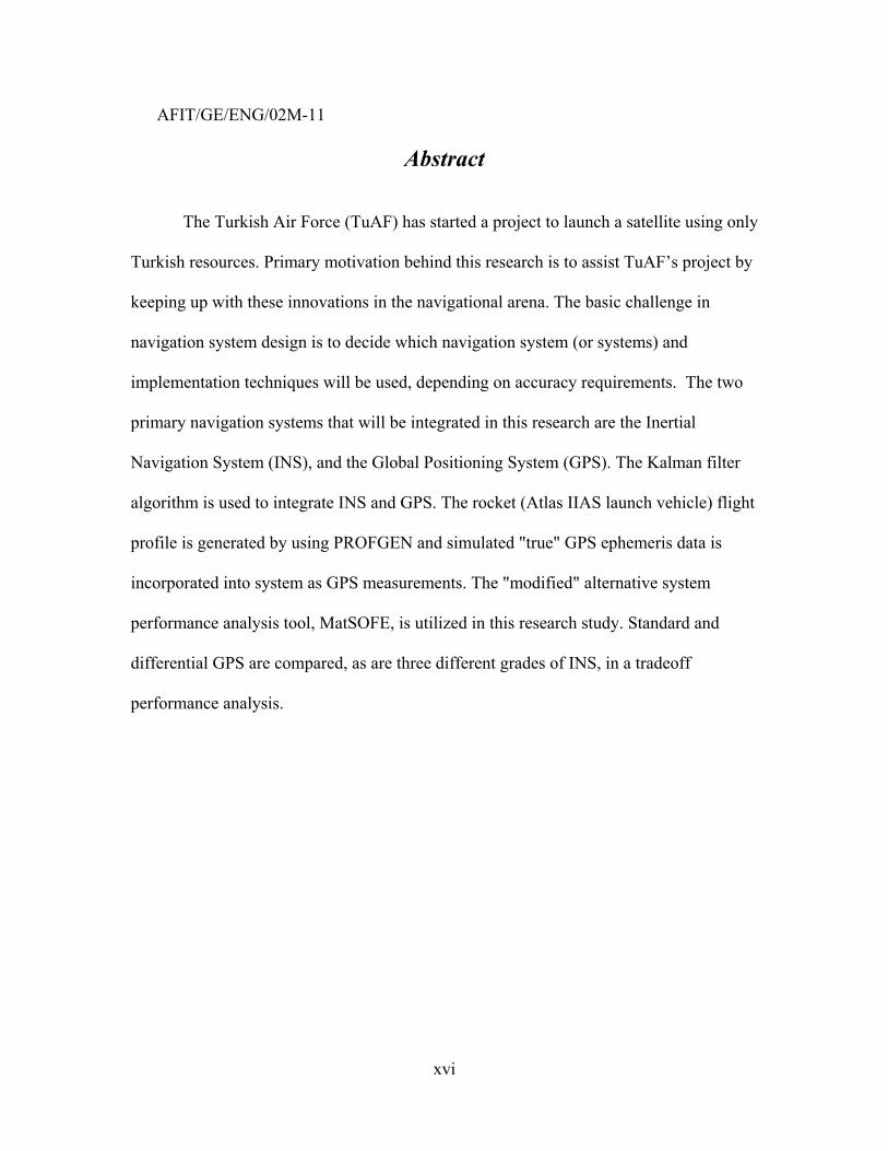
Abstract
The Turkish Air Force (TuAF) has started a project to launch a satellite using only
Turkish resources. Primary motivation behind this research is to assist TuAF’s project by
keeping up with these innovations in the navigational arena. The basic challenge in
navigation system design is to decide which navigation system (or systems) and
implementation techniques will be used, depending on accuracy requirements. The two
primary navigation systems that will be integrated in this research are the Inertial
Navigation System (INS), and the Global Positioning System (GPS). The Kalman filter
algorithm is used to integrate INS and GPS. The rocket (Atlas IIAS launch vehicle) flight
profile is generated by using PROFGEN and simulated "true" GPS ephemeris data is
incorporated into system as GPS measurements. The "modified" alternative system
performance analysis tool, MatSOFE, is utilized in this research study. Standard and
differential GPS are compared, as are three different grades of INS, in a tradeoff
performance analysis.
xvi
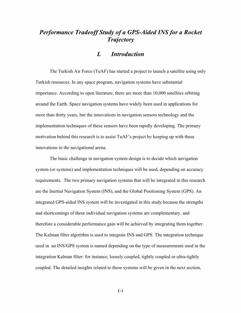
Performance Tradeoff Study of a GPS-Aided INS for a Rocket Trajectory
I. Introduction
The Turkish Air Force (TuAF) has started a project to launch a satellite using only
Turkish resources. In any space program, navigation systems have substantial
importance. According to open literature, there are more than 10,000 satellites orbiting
around the Earth. Space navigation systems have widely been used in applications for
more than thirty years, but the innovations in navigation sensors technology and the
implementation techniques of these sensors have been rapidly developing. The primary
motivation behind this research is to assist TuAF’s project by keeping up with these
innovations in the navigational arena.
The basic challenge in navigation system design is to decide which navigation
system (or systems) and implementation techniques will be used, depending on accuracy
requirements. The two primary navigation systems that will be integrated in this research
are the Inertial Navigation System (INS), and the Global Positioning System (GPS). An
integrated GPS-aided INS system will be investigated in this study because the strengths
and shortcomings of these individual navigation systems are complementary, and
therefore a considerable performance gain will be achieved by integrating them together.
The Kalman filter algorithm is used to integrate INS and GPS. The integration technique
used in an INS/GPS system is named depending on the type of measurements used in the
integration Kalman filter: for instance, loosely coupled, tightly coupled or ultra-tightly
coupled. The detailed insights related to these systems will be given in the next section,
I-1
but these terms will be briefly described here. Loosely coupled systems are integrated at
the navigation solution level. Both INS position data and GPS position data are taken into
the Navigation Kalman filter. Tightly coupled systems are integrated at the pseudorange
level, and ultra-tightly coupled systems at the in-phase and quadrature (I and Q) signal
level. In this study the tightly coupled integration technique will be used to integrate INS
and GPS. The justifications for this choice will be presented in the background section.
It is believed that an integrated INS/GPS system can meet and exceed both the
navigation accuracy and integrity requirements for a satellite to launch. In this study, the
author will investigate the performance of different types and navigation accuracies of
GPS-aided INS systems, and make a tradeoff analysis between their cost, applicability,
accuracy, implementation ease, etc. To achieve this goal, 6 different cases, each case
involving a separate GPS-aided INS system with different navigation accuracies, were
constructed.
This research investigates only the navigation aspect of space navigation systems.
The study of designing a control algorithm for a space vehicle could also be studied, but
it is considered as the follow-on step, and will not be discussed in this thesis.
1.1 Background
The inertial sensors, like accelerometers and gyros, used in an INS have some
errors with stochastic properties. These errors tend to increase over time (long-term
instability) with unbounded position error growth and require occasional or continual
compensation [17: 526]. Its autonomous navigation capability makes INS the primary
navigation system in most applications. It does not need any external aid to navigate, but
I-2
its accuracy can be improved by using navigational aids (GPS, TACAN, RADAR, etc.).
On the contrary, GPS alone does not provide an adequate solution either, “due to low
output rate of GPS receivers and the need for redundant information during GPS system
failures or simple loss of GPS measurements [44: 2932] ”. GPS has long-term accuracy,
but is sensitive under highly dynamic conditions, such that the number of tracked
satellites may fall below four, which means the GPS receiver can no longer generate a
navigation solution on its own. The integrated INS/GPS system not only provides a very
efficient means of navigation due to the short-term accuracy of INS combined with the
long-term accuracy of GPS, but also produces a system with performance that exceeds
that of the individual sensors.
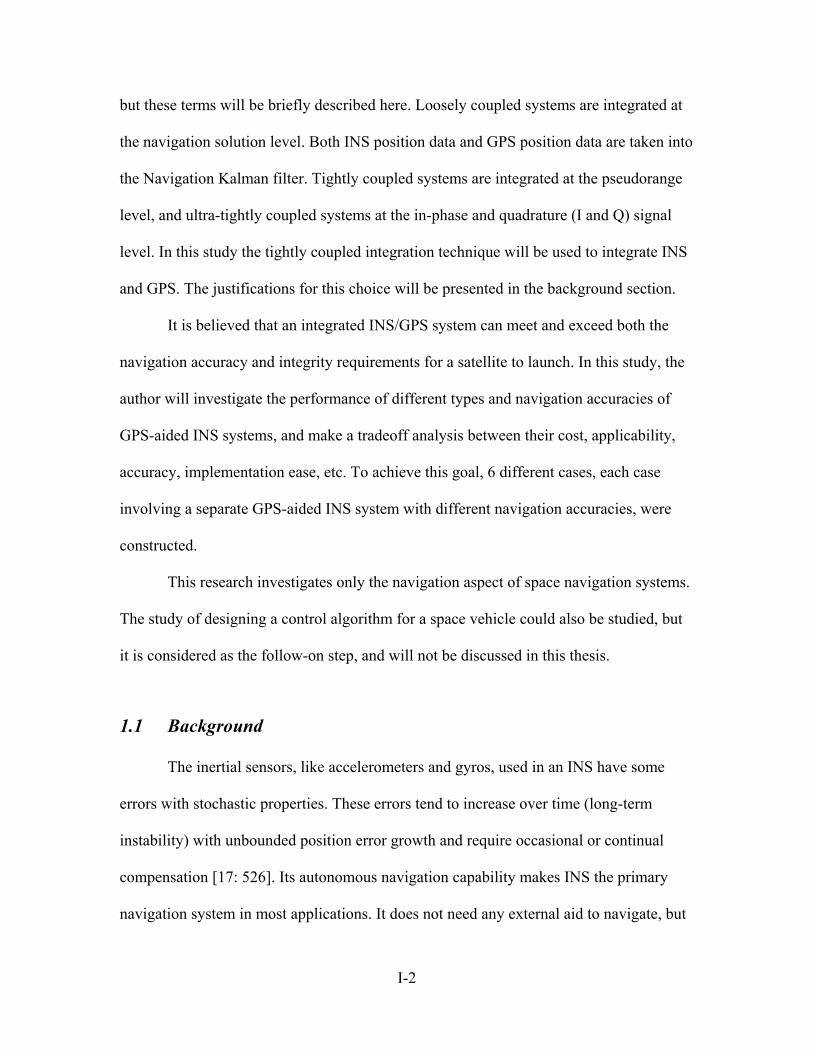
There are several options to integrate the GPS and INS sensors. Among these
options, two traditional integration techniques are widely used in applications: loosely
coupled (Figure I-1) and tightly coupled (Figure I-2). In the open literature, there are
numerous navigation system designs using these techniques. Both have advantages and
disadvantages.
In a loosely coupled system, the INS integration Kalman filter uses GPS-derived
position and velocity (the output of a GPS Kalman filter) as a measurement. Loosely
coupled integration treats GPS and INS as individual navigation systems, combining the
two at the navigation solution level. Raw GPS data is processed first by a Kalman filter,
and the integration Kalman filter is then applied to combine INS and GPS navigation
solutions. Often only the INS error states are modeled explicitly in the integration
Kalman filter. That does not mean that GPS is assumed error-free, only that the dynamic
characteristics of the GPS errors are not compensated by the integration filter. The GPS
I-3
GPS receiver
INS KALMAN FILTERUncorrected
PositionVelocity, &Attitude
Corrected PositionVelocity, &Attitude
GPS Kalman Filter
GPSGPS navigationsolution
Figure I-1. Loosely coupled INS/GPS integration
GPS
INS
KALMAN FILTER+
_
+_
Uncorrected PositionVelocity, &Attitude
Pseudorange
INS Pseudorangecalculations
Estimated position, Velocity & attitude
errors
Corrected PositionVelocity, &Attitude
GPSephemeris
data
Figure I-2. Tightly coupled INS/GPS integration
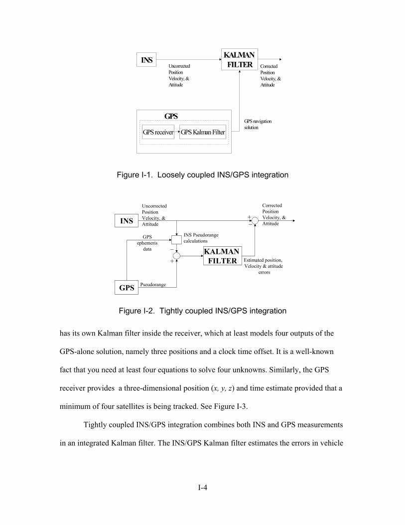
has its own Kalman filter inside the receiver, which at least models four outputs of the
GPS-alone solution, namely three positions and a clock time offset. It is a well-known
fact that you need at least four equations to solve four unknowns. Similarly, the GPS
receiver provides a three-dimensional position (x, y, z) and time estimate provided that a
minimum of four satellites is being tracked. See Figure I-3.
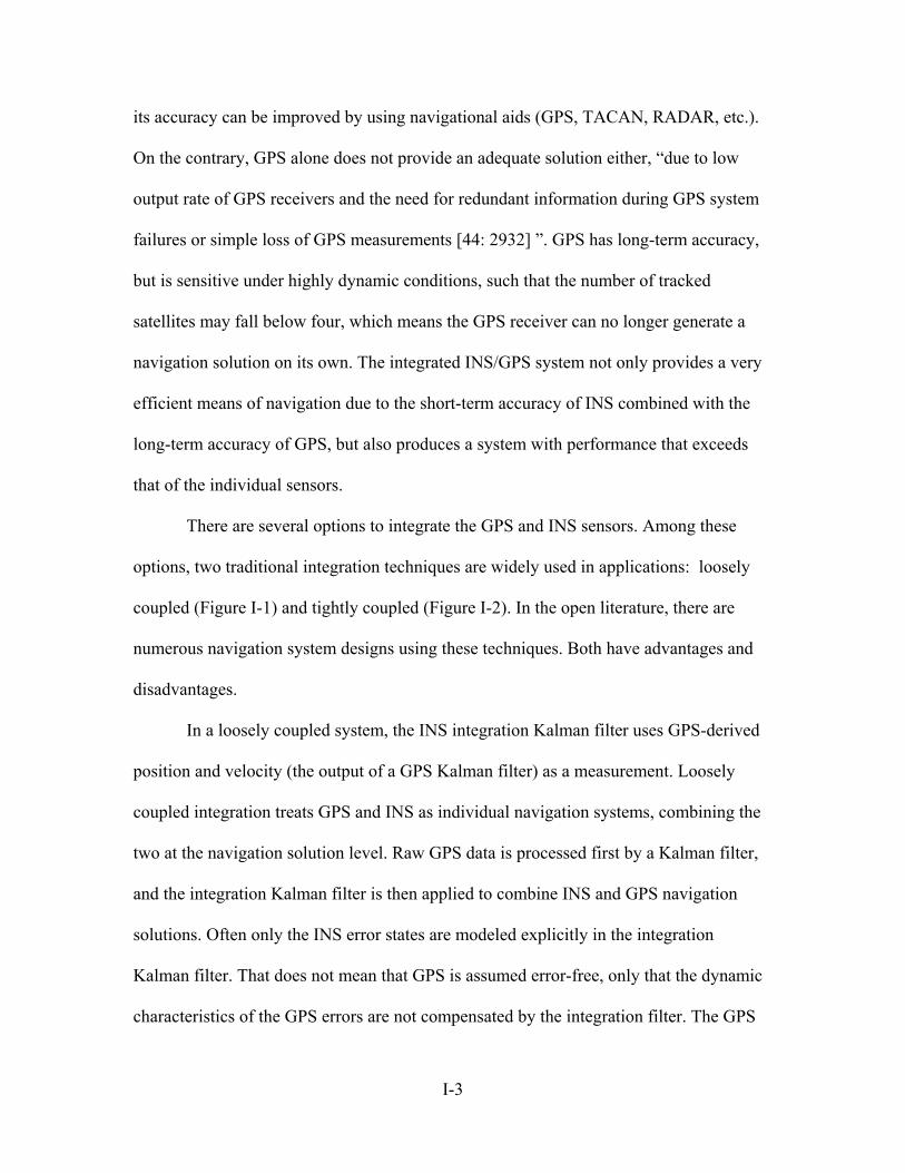
Tightly coupled INS/GPS integration combines both INS and GPS measurements
in an integrated Kalman filter. The INS/GPS Kalman filter estimates the errors in vehicle
I-4
b
RN
R1
Ri
(xi ,yi , zi )
b bias clock receiver and z)y,,position(x user for solve4, N If
N ., 4, 3, 2, 1, i bzzyyxxR
(known) positions Satellite:) z ,y ,x (nts)(measureme esPseudorang : R
iiii
iii
i
≥…=
−−+−+−= 222 )()()(
Figure I-3. The Principle of Satellite Navigation [25]
position, velocity and attitude along with Inertial Measurement Unit (IMU) errors, such
as gyro drift, and accelerometer bias, and GPS errors, such as clock bias and drift rate, by
using both INS position solution and GPS pseudorange measurements [41: 773]. Thus,
the integration is performed at the pseudorange measurement level rather than at the GPS
navigation solution level. Only one Kalman filter is applied in this integration technique.
Positioning is performed on the basis of both INS and GPS measurements, even if the
number of tracked satellites falls below four. Since they are integrated at the raw in-phase
and quadrature phase (I & Q) signal level and provide a position estimate with an
accuracy of cm level, and are still under development, ultra-tightly coupled systems are
not considered as a concern of this study. Additionally, since the desired position
accuracy of a launch vehicle is about 50-80 meters, the author decided not to consider
ultra-tightly coupled systems in this study.
I-5
There are three main GPS types, depending on GPS receiver range solution
technique: (1) Standard GPS, (2) Code Range Differential (DGPS), and (3) Carrier Phase
DGPS. For the military applications their Two-Dimensional Distance Root Mean Square
(2 DRMS) horizontal position accuracies are approximately 6 m., 1-3 m., and 1-2 cm.,
respectively [34]. 2 DRMS is the root mean square (RMS) of the two-dimensional
distance error ( ( ) nyx =DRMSn
1i
2i
2i ÷
+∑=
). The probability of being inside
2xDRMS circle varies between 95% and 98% (depending upon ratio of xσ and yσ ).
The basic difference between them is the type of information which the GPS receiver
uses to generate a navigation solution. The incoming GPS signal consists of three
components: carrier (RF sinusoidal signal, which is usually called phase, or carrier
phase), ranging code (basically zeros and ones, and briefly called code or PRN code),
and navigation data (a binary coded message) [25]. The differential GPS technique takes
advantage of the error correlations between multiple receivers. Its accuracy is anywhere
between 5 m. and 1 cm., depending upon the method used. Obviously, carrier phase
DGPS provides the highest precision when compared to the others [34]. Taking the
accuracy requirements of a launch vehicle into account, the research cases related to
carrier-phase DGPS-aided INS systems are removed from the research scope. It was
obvious that carrier-phase DGPS would provide much more accuracy than what is
needed. Detailed information related to GPS, DGPS, and Carrier-Phase GPS can be
found in Key Terms (next page) and Chapter 2.4 of this study.
I-6
1.2 Key Terms
Inertial Navigation System (INS): A self-contained, dead reckoning precision
navigation system, which uses inertial sensors, such as gyroscopes and accelerometers, to
provide navigation information. Typical accuracy: 0.4-4.0 nautical miles/hour circular
error probable (CEP). CEP defined as radius of a circle inside which half of the points
(errors) fall ( ) % 3 ) + ( 0.59 = CEP yx ±σσ .
Global Positioning System (GPS): A passive, space-based, universal and accurate
source of navigation information (three-dimensional position and velocity) and time. The
system has been designed, developed, and maintained by the U.S. Department of
Defense (DoD) [6,9,10,44]. Accuracy: Stand-Alone GPS is typically 6 meters (military,
dual frequency) and 10 meters (civilian) approximate horizontal accuracy (2DRMS) [34].
Differential GPS (DGPS): A ground-based GPS receiver (accurately surveyed)
uplinks error corrections to nearby vehicles to be positioned. DGPS takes advantage of
the correlation of errors between receivers. The errors associated with the worst error
sources are similar for users located “not far” from each other, and they change slowly in
time. In other words, errors are correlated both spatially and temporally. Clearly, an error
in a measurement can be estimated and removed up to a certain level by using proper
DGPS techniques, if the location is known [25]. Accuracy: 1-5 meters, depending upon
method used [34].
Carrier-Phase DGPS: A very popular and accurate receiver technique, which is
able to measure the incoming satellite-transmitted GPS signal to a fraction of a
wavelength. Accuracy: 1-2 centimeter [10, 34].
I-7
Kalman Filter: A recursive computer algorithm that uses sampled-data
measurements to produce optimal state estimates of a dynamical system, under the
assumptions of linear system models and white Gaussian noise models. Developed by
R.E. Kalman in the early 1960s, A New Approach to Linear Filtering and Prediction
Problems [16].
Barometric Altimeter: An altimeter designed to output altitude relative to the
pressure difference. They are cheap and widely used as vertical channel aid to INS
because of the inherent instability of the vertical channel in an unaided INS [10].
1.3 Literature Review
The following is a brief discussion of the literature reviewed for this research,
process, which covers NASA technical reports, previous Air Force Institute of
Technology (AFIT) theses, text books, course handouts, and IEEE transactions and
conferences related to the INS/GPS integrated navigation system and its space
applications. The reviewed sources will be presented in following categories
1.3.1 Benefits of Integrated Systems
The inertial sensors used in an INS have some errors and these errors tend to
increase by time. They have to be compensated occasionally or frequently. Although an
INS provides good high-frequency navigation information, it has considerable long-term,
low frequency errors due to the physical gyro drift rate problem. The use of navigational
aids, like GPS and a barometric altimeter, can significantly enhance the navigation
accuracy of an INS.
I-8
All of the GPS range solution techniques (either stand-alone or differential) suffer
from some inadequacy. The most significant are:
• The data rate of GPS receiver is too low for many applications;
• High DGPS accuracy is limited by the distance between the reference
station and the user because of the errors associated with the ionosphere,
which make it difficult to determine the integer ambiguity resolution on-
the-fly [13];
• Influences of high acceleration on the receiver clock, code tracking loop
(delay lock loop) and carrier phase loop may become considerable; these
tracking loops are used to provide estimates of tracking errors for signal
processing purposes in a GPS receiver;
• Signal loss-of-lock and cycle slips may occur very frequently due to
aircraft high dynamics and other causes [35: 18-12].
INS/GPS integration has proven to be a very efficient means of navigation due to
the short term accuracy of INS combined with the long term accuracy of GPS fixes
[4,7,8,17,35,41]. INS/GPS integration is the optimal solution to the navigation problem
rather than using either system alone, since the Kalman filter includes effects of both
GPS and INS errors. “Many researchers have studied the methodology of combining
these two navigation sensors. Navigation employing GPS and INS is a synergistic
relationship. The integration of these two types of sensors not only overcomes
performance issues found in each individual sensor, but also produces a system whose
performance exceeds that of the individual sensors.” [17: 526].
I-9
INS and GPS are complementary technologies in the sense that the weakness of
one is the strength of another. Integration of INS and GPS leads to a particularly
attractive and robust system that can produce better navigation information compared to
either one.
1.3.2 INS/GPS Integration Techniques
“There are many options to integrate the INS and GPS onboard the spacecraft.
The first integration option, also the simplest implementation technique, is resetting the
position and velocity output of INS with that of GPS. This option was selected as the
baseline INS/GPS integration approach on the NASA/TRW orbit maneuvering vehicle
(OMV) [41].”
The second option, called loosely coupled or cascaded integration, basically takes
the output of a GPS Kalman filter (position and velocity solution) as measurements into
integration Kalman filter. This integration behaves like an INS alone system in case of
GPS outages.
The third integration option, called tightly coupled INS/GPS integration,
combines the GPS pseudorange and/or range rate measurement and INS raw
measurements in an integration Kalman filter. Having only one Kalman filter is not the
only difference between loosely and tightly coupled systems. The fundamental difference
is using raw measurements instead of the navigation solution for GPS. The INS/GPS
integration Kalman filter estimates the errors in spacecraft position, velocity and attitude
along with the inertial measurement unit (IMU) instrument errors, such as gyro drift and
accelerometer bias and scale factor. This tightly coupled integration option gives the best
I-10
navigation accuracy of the three techniques just discussed, and it does not suffer from the
filter-driving-filter (the GPS receiver Kalman filter-driving-integration Kalman filter)
stability concern of the loosely coupled approach [41, 23].
An additional literature review was also conducted to find out whether anything
new, especially in the GPS portion of the navigation system and its application in space
navigation area, had been accomplished that would provide different, or additional,
models to be incorporated into this research. In NASA’s technical reports and contractor
reports, it is seen that the accuracy expected from a space navigation system (GPS-aided
INS and some navigational aids, such as barometric altimeter, star tracker, etc.) is in the
level of 50 meters per channel CEP [26,40].
1.3.3 Integration Kalman Filter Error and Measurement Models
Once the error models for the navigational systems are determined, the rest of the
Kalman filter design is relatively straightforward. Navigational systems (GPS, INS,
barometric altimeter, etc.) error models are named depending on their state number, for
instance, an 11-state INS error model or a 30-state GPS error model. Each state within
that specified number of states represents a specific sensor error, which we want the
Kalman filter to estimate and compensate. The previous AFIT theses accomplished by
Gray [10], Britton [6], and White [44], guided this part of literature review. Actually,
Gray’s thesis was the basis for the other two. The error models and measurement models
they used have been analyzed and validated for almost ten years in AFIT theses. These
models have proven their accuracy in many applications. However, to be 100% confident
about the truthfulness of these models, they are checked once again and matched with the
I-11
information available in Performance Accuracy (Truth Model/Error Budget) Analysis for
the LN-93 Inertial Navigation Unit documentation [18]. The detailed INS, GPS,
barometric altimeter error and measurement models will be delineated in Chapter 3 of
this study.
1.3.4 The Chosen Launch Vehicle (Atlas IIAS) for Simulations
To accomplish this study, both the GPS and the INS data have to be generated and
inserted into the simulation environment. A Fortran-based Flight Profile Generator
(PROFGEN) generates the INS data for the rocket flight trajectory [29]. PROFGEN is
capable of providing 53 different output variables to the user, and the user can choose the
preferred number of output variables. To run this Profile Generator, one has to have the
vehicle flight characteristics (take-off coordinates, vehicle initial heading, checkpoints,
flight lengths, etc.) in hand and has to put those data into profile input (PROF_IN) file.
Detailed information concerning PROFGEN and rocket flight profile generation
procedures will be presented in Section 3.3 and 4.2 of this study. As a result of personal
interview with Dr. Tregesser [39] from the aerospace department and the reviewed
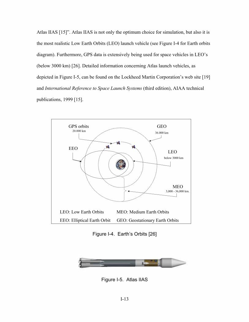
literature [15,19], the Atlas IIAS launch vehicle (Figure I-5) was chosen as the
“optimum” in terms of applicability, cost, orbit specifications, flight statistics and thrust
[15]. The operational Atlas II family is one of the largest commercial launch vehicles in
the United States and is currently operating with a 100% mission success rate. As of
June 19, 2001, Atlas IIAS has achieved 22 for 22 successful missions, for a total of 55
consecutive successful Atlas flights [15]. “Based on open-source information, the Federal
Aviation Administration (FAA) estimates $ 90-105 million price range for commercial
I-12
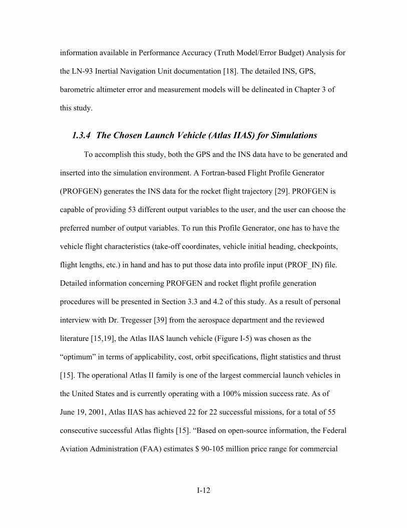
Atlas IIAS [15]”. Atlas IIAS is not only the optimum choice for simulation, but also it is
the most realistic Low Earth Orbits (LEO) launch vehicle (see Figure I-4 for Earth orbits
diagram). Furthermore, GPS data is extensively being used for space vehicles in LEO’s
(below 3000 km) [26]. Detailed information concerning Atlas launch vehicles, as
depicted in Figure I-5, can be found on the Lockheed Martin Corporation’s web site [19]
and International Reference to Space Launch Systems (third edition), AIAA technical
publications, 1999 [15].
MEO3,000 - 36,000 km.
EEOLEO
below 3000 km
GEO 36.000 km
LEO: Low Earth Orbits MEO: Medium Earth Orbits
EEO: Elliptical Earth Orbit GEO: Geostationary Earth Orbits
GPS orbits20.000 km
Figure I-4. Earth’s Orbits [26]
Figure I-5. Atlas IIAS
I-13
1.4 Problem Statement
As mentioned previously, this study has started with examining the theses
accomplished by former AFIT students Robert A. Gray [10], Capt. Ryan Britton [6], and
2nd Lt Nathan White [44]. These theses are concerned with accurate GPS/INS
integrations for a precision landing or airborne navigation application, rather than for a
satellite launch. It has seen that the truth models and filter design error models they used
for INS and GPS have been utilized in AFIT for more than 8 years as validated models,
and consequently the author decided to use these models in this research.
This research will concentrate on performances of different types and accuracies
of GPS-aided INS systems and will make a tradeoff analysis between their cost,
applicability, accuracy, implementation ease, etc. to assist TuAF’s space project. The
tradeoff study will be accomplished based on the performance analysis between 6
differently constructed cases. Each case represents a tightly coupled integration of these
two types of GPS (standard single-receiver GPS, dual frequency P-code DGPS) with
three grades of INS (0.4, 2.0, and 4.0 nm/hr CEP INS). These three grades of INS’s
represent military grade, commercial grade, and less expensive (possible MEMS in a few
years) Inertial Navigation Systems. The constructed cases are shown in Table I-1.
In Cases I and II, the 0.4 nm/hr CEP INS will be integrated with two different
accuracies of GPS data, namely standard single-frequency stand-alone GPS, and P-code
DGPS. Cases III through IV and Cases V through VI achieve the same integrations for
2.0nm/hr CEP, and 4.0 nm/hr CEP INS’s, respectively.
I-14
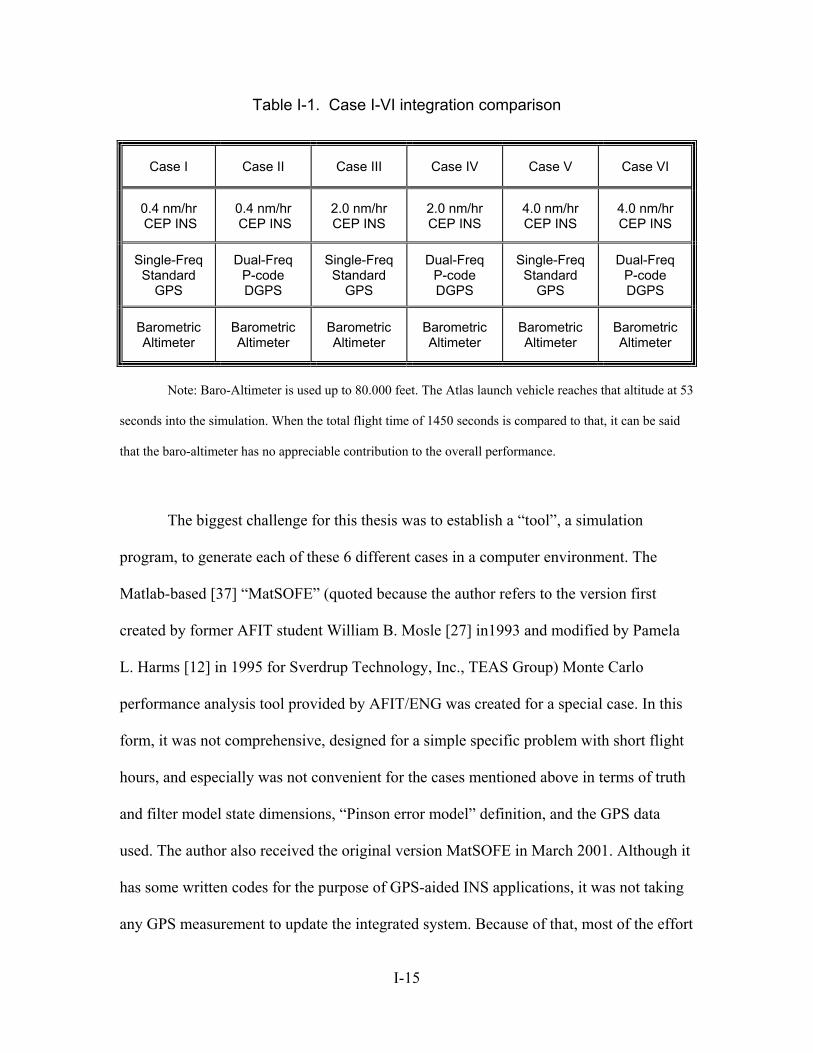
Table I-1. Case I-VI integration comparison
Case I Case II Case III Case IV Case V Case VI
0.4 nm/hr CEP INS
0.4 nm/hr CEP INS
2.0 nm/hr CEP INS
2.0 nm/hr CEP INS
4.0 nm/hr CEP INS
4.0 nm/hr CEP INS
Single-Freq Standard
GPS
Dual-Freq P-code DGPS
Single-Freq Standard
GPS
Dual-Freq P-code DGPS
Single-Freq Standard
GPS
Dual-Freq P-code DGPS
Barometric Altimeter
Barometric Altimeter
Barometric Altimeter
Barometric Altimeter
Barometric Altimeter
Barometric Altimeter
Note: Baro-Altimeter is used up to 80.000 feet. The Atlas launch vehicle reaches that altitude at 53
seconds into the simulation. When the total flight time of 1450 seconds is compared to that, it can be said
that the baro-altimeter has no appreciable contribution to the overall performance.
The biggest challenge for this thesis was to establish a “tool”, a simulation
program, to generate each of these 6 different cases in a computer environment. The
Matlab-based [37] “MatSOFE” (quoted because the author refers to the version first
created by former AFIT student William B. Mosle [27] in1993 and modified by Pamela
L. Harms [12] in 1995 for Sverdrup Technology, Inc., TEAS Group) Monte Carlo
performance analysis tool provided by AFIT/ENG was created for a special case. In this
form, it was not comprehensive, designed for a simple specific problem with short flight
hours, and especially was not convenient for the cases mentioned above in terms of truth
and filter model state dimensions, “Pinson error model” definition, and the GPS data
used. The author also received the original version MatSOFE in March 2001. Although it
has some written codes for the purpose of GPS-aided INS applications, it was not taking
any GPS measurement to update the integrated system. Because of that, most of the effort
I-15
was spent to modifying the simulation code and writing new code, depending on needs
for each integration case. By January 2002, the MatSOFE has reached its present, revised
form. The current version of MatSOFE is capable of taking real GPS satellite vehicle
ephemeris data by using the System Effectiveness Model for Windows Version 3.6.4.
(WSEM 3.6) software [2] for measurement updates. Also, the UD covariance
factorization filter principles, developed by Bierman and Thorton [20: 392], were
incorporated for propagation and measurement update cycles. U-D factorization
algorithm increases the numerical stability in the Kalman filter. The 39-state reduced
truth model of Litton 93-state (LN-93) INS [18], which is the most common INS in the
market and being used by the F-16 Fighting Falcon aircraft, is also integrated into current
version. Detailed information about MatSOFE, error states, Pinson error model, real GPS
satellite vehicle ephemeris data, WSEM software program and LN-93 INS definitions
will be presented in next chapter.
Even though most of the reviewed subjects were familiar and studied during my
AFIT academic education, many additional insights related to INS, GPS, and their
integration techniques were gained in the literature review phase. Those insights will be
used during both the simulation and tradeoff analysis phase.
I-16
1.5 Assumptions
All theses are limited by the assumptions made, and no research can be
adequately evaluated unless these assumptions are clearly defined [27]. This section
outlines the assumptions that have been made in this thesis [10].
i. All work is to be conducted through computer simulation. “Real
world” data is neither collected nor used in the simulations. Instead, all “real
world” measurements are accurately simulated. There is true satellite vehicle
ephemeris data within the WSEM 3.6 software, but the actual GPS
measurements themselves are simulated in the computer environment. The
emphasis here is on the model representing the real world conditions in the
filter design. The real world data used in the simulation is modeled with a full-
order truth error state model. MatSOFE provides a Monte Carlo analysis of a
GPS-aided INS Kalman filter design as seen in a realistic “truth model”
environment. The full-order “truth models” and reduced-order “filter design
models” are presented clearly in Chapter 3 of this thesis study.
ii. The INS will not have the usual 8-minute ground alignment. That
feature could be implemented into MatSOFE, but because of the time
constraints it is left as a future addition to MatSOFE.
iii. The LN-93 INS system has the natural ability of updating the vertical
channel with barometric altimeter output. MatSOFE reflects that characteristic
as well. The use of barometric altimeter is included in the modeling of the
system, so that the INS platform is assumed to be stabilized with a barometric
altimeter. Without a vertical channel aiding device, the INS vertical channel is
I-17
unstable. In fact, using a barometric altimeter as a vertical channel aid is not
the only option, but it is the cheap and the most commonly used method.
Unlike GPS aiding, it is not vulnerable to jamming or spoofing.
iv. Also, the barometric altimeter is assumed to be good up to 80,000 feet
altitude. Rapid altitude change during the launch is expected, and at 80,000
feet the baro-altimeter will be turned off (in simulations, that happens almost
at 53 seconds).
v. The computer-simulated Atlas IIAS launch vehicle profile is generated
by using the software “PROFGEN” [29]. PROFGEN has been developed to
work with MatSOFE [12] to provide the necessary data files to simulate
rocket dynamics. The actual total flight hour for the Atlas is just about 4000
seconds up to perigee entrance. For simplicity and saving computer memory,
the flight lasts until second main engine cut off (MECO2). In fact, at about
500 seconds, the rocket is on the orbit and after that point it makes the perigee
entrance maneuver. The MatSOFE and PROFGEN are presented in Chapter 3
of this study in details.
vi. In the constructed cases, it is assumed that there will be no GPS
measurement outage or failure, because in a space vehicle INS and GPS
systems will always be redundant. In reality, from the GPS satellite vehicles’
point of view (i.e., with respect to the geometry of the satellites and receiver
onboard the rocket), GPS data will almost always be available for LEO space
vehicles.
I-18
vii. A 4.0 nm/hr CEP INS is assumed as representative of a “micro
electromagnetic system (MEMS)” INS. Actually nowadays, their accuracy is
almost 6.0 nm/hr CEP, but when this thesis is finished, or shortly thereafter, it
is probable to have MEMS INS units with 4.0 nm/hr CEP accuracy. 0.4 nm/hr
CEP and 2.0 nm/hr CEP INS’s represent current higher and medium accuracy
INS’s respectively.
viii. A sample period of one second has been chosen for the EKF. As a
matter of fact, the decision to use a one-second sample period is based
primarily on the typical availability of the GPS measurement in the real world.
The sample period refers to how often the GPS measurements will be brought
into the EKF. The United States Coast Guard Navigation Information Service
Bulletin Board distributes post-fit ("precise") GPS orbital ephemeredes
("orbits") computed by National Oceanic and Atmospheric Administration’s
(NOAA) National Geodetic Survey (NGS) in two formats. These formats are
known as EF18 and SP3. EF18 is a binary file, while SP3 is its ASCII
equivalent [32]. Usually, the GPS EF18 and SP3 almanac files used in this
study are stored ever 15 minutes or at a higher sample period, and they need to
be converted to a different format to alter the sample period. The one-second
period of GPS data used in this thesis is obtained by means of the software
used to convert EF18 data format into SP3 data format. Though faster GPS
outputs are available via “utility software” [32], a one second sample period is
chosen as a good, representative design choice.
I-19
ix. The computer simulations have been developed using a program called
MatSOFE, which has been updated and upgraded by the author. MatSOFE is
the Matlab [37] version of the Fortran-based Multi-mode Simulation for
Optimal Filter Evaluation (MSOFE) [30]. MSOFE is well-established Air
Force software to develop and test linear and extended Kalman filter
algorithms.
x. The sv ephemeris data using WSEM 3.6 software program was
downloaded from the ARINC, Inc. web page[2]. The ephemeris data is then
post-processed by the utility software programs obtained from NOAA’s
National Geodetic Survey web page [32] .
xi. Only four GPS satellites were modeled in MatSOFE. In real-world
applications, depending on the receiver position on Earth, most likely 6-8
satellites would be visible at a certain time epoch. Four SV are always
available. The SEM 3.6 software selects the four best satellites available at a
given time based on an average Position Dilution of Precision (PDOP) less
than 1.3 and these satellites are used without interruptions.
xii. The MatSOFE runs are conducted using 15-run Monte Carlo analyses.
While a larger batch size for the Monte Carlo analysis would be preferable,
this value has been chosen to keep the computational burden of the thesis
within reasonable bounds, while maintaining adequate confidence that the
resulting sample statistics properly reflect the true statistics [10].
xiii. Flight segment durations and accelerations of the real launch vehicle
were accurately incorporated in order to generate the Atlas profile
I-20
realistically. It is also assumed to be launched from Cape Canaveral AS,
SLC-41( ). Available orbit inclinations for that location are
and polar 90 . The author picked inclination orbit as a
fair choice.
WN 00 0.81,5.28
00.5505.28 − 00. 05.28
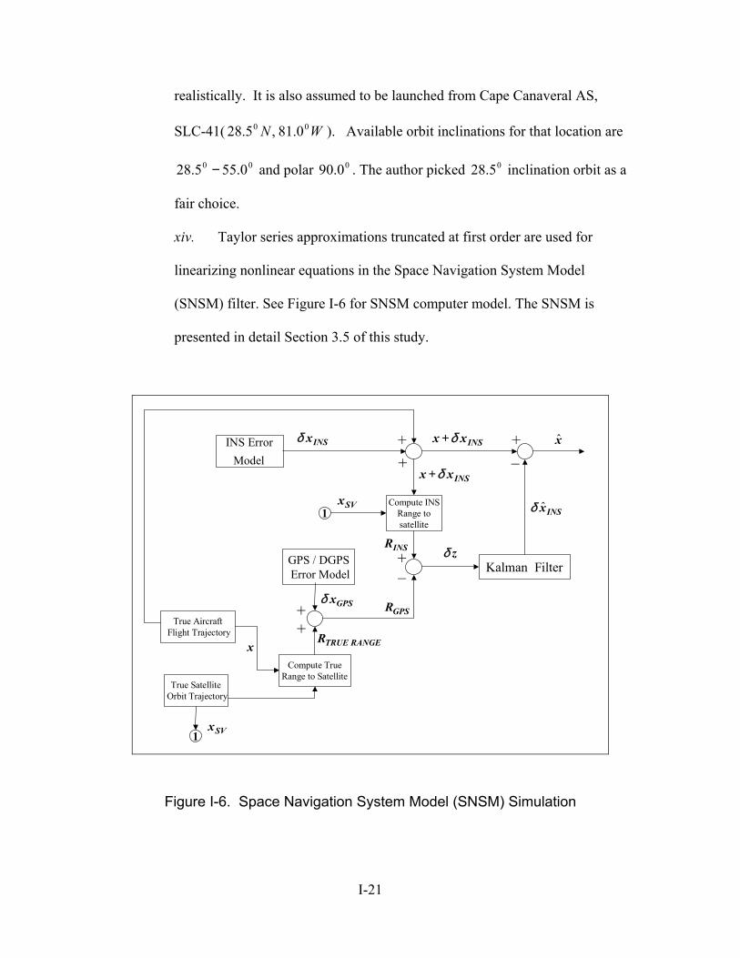
xiv. Taylor series approximations truncated at first order are used for
linearizing nonlinear equations in the Space Navigation System Model
(SNSM) filter. See Figure I-6 for SNSM computer model. The SNSM is
presented in detail Section 3.5 of this study.
Kalman Filter
INS ErrorModel
GPS / DGPSError Model
Compute INSRange to satellite
True SatelliteOrbit Trajectory
True AircraftFlight Trajectory
1
INSxδ INSxx δ+
INSxx δ+
INSxδ
GPSxδGPSR
RANGETRUER
SVx
zδ
x
1
Compute TrueRange to Satellite
SVx
INSR
x
++
+
++
+
_
_
Figure I-6. Space Navigation System Model (SNSM) Simulation
I-21
1.6 Scope
This research will focus on a simulation-based tradeoff analysis study of
GPS/DGPS integrated with a baro-inertial navigation system for the Atlas IIAS launch
vehicle. The study of designing a control algorithm for a launch vehicle could also be
studied, but it is considered as the follow-on step.
To accomplish the tradeoff performance analysis of a GPS-aided INS system, one
has to make Monte Carlo simulations and/or covariance analyses. MSOFE (Multimode
Simulation for Optimal Filter Evaluation (MSOFE) software [30]) is restricted for use by
U.S. government agencies and their U.S. contractors. In order to accomplish the analyses,
the Matlab-based [37] “MatSOFE” (first created by former AFIT student William B.
Mosle [27] in 1993 and modified by Pamela L. Harms [12] in 1995 for Sverdrup
Technology, Inc., TEAS Group and finally upgraded and modified by the author) is used
as an evaluation software. Not being a compiled language, like Fortran or C, MATLAB
causes MATSOFE to be almost eight times slower than MSOFE. This means long run
times. (In the simulation phase, it is seen that a 15-Monte Carlo-run simulation takes 8 to
20 hours, depending on the processor speed of the computer being used.) When this
constraint is taken into account, accomplishing only the navigational aspect of a space
guidance, navigation, and control system becomes a more reasonable scope for this
research.
The tasks involved in this research are as follows:
1. Review prior AFIT theses of Negast [33], Mosle [27], Gray [10], Britton [6],
and White [44]. Investigate the INS/GPS integrations used in their research.
I-22
2. Conduct a literature review concerning the latest innovations in GPS range
resolution and recent INS/GPS integration techniques.
3. Study, and if necessary restructure, the current “truth model”: a complete,
complex mathematical model that portrays true system behavior very
accurately. Justify its sustained use and, update the GPS/DGPS information.
4. Make any adjustments that are required to yield an accurate, validated model.
5. Further validate the truthfulness of the present “truth model” by comparing it
to Litton-93 documentation [18].
6. Start simple. First understand the basic principles of the provided MatSOFE
software.
a. Fill the gaps of the provided MatSOFE. Add/rewrite the necessary m-
files (matlab script files).
b. First generate The KC-135 Tanker aircraft flight profile by using the
provided PROF_IN file (the input file of PROFGEN describing the
desired maneuvers, flight segments, accelerations, etc of the vehicle
that was used in previous research) in Gray’s thesis [10].
c. Make necessary changes in the simulation code in order to take “true”
GPS measurement data evaluated by WSEM 3.6 software into the
integrated system. Put the GPS satellite vehicle ephemeredes data into
a format that Matlab can load it into simulation.
d. Incorporate the UD covariance factorization filter principles to
propagation and measurement update cycles in order to increase the
numerical precision and stability in the Kalman filter.
I-23
e. Merge FLY_OUT (PFOFGEN output in formatted form) and SV_data
(final form of processed GPS satellite vehicle (SV) measurements in
Litton ECEF coordinates) into a single INPUT file for MatSOFE.
7. Compare MatSOFE results to Mosle’s, Gray’s and Britton’s MSOFE results
[6,10,27] to demonstrate that the upgraded MatSOFE is a reliable and easy-to-
learn navigation systems performance evaluation tool.
8. Carry out a literature review to decide upon an optimum performance launch
vehicle to be used in the simulation. Clearly identify the characteristics of
launch vehicle to generate a realistic flight simulation.
9. Perform a Monte Carlo analysis for each suggested case.
10. “Tune” the filter to provide the best possible performance.
11. Analyze each case and compare the results of one to another.
1.7 Summary
This chapter has given a brief overview of the thesis plan to develop an
integrated GPS/DGPS, INS, and Barometric Altimeter integrated system for navigation
of a rocket launching a satellite. The background for the necessity of such a system, the
various system integrations, past research, the project scope, and all assumptions have
been presented. The reference frames used in this research, as well as the INS, GPS,
DGPS, and barometric altimeter subsystems are presented in Chapter 2, along with a
discussion of Kalman filter algorithms. Chapter 3 introduces MatSOFE and PROFGEN,
and presents the SNSM system and filter models. Chapter 4 presents the results and
analysis of the SNSM. Chapter 5 presents conclusions and recommendations.
I-24
II. Theory
2.1 Introduction
The background presented in this section includes the basic theory on a ring laser
gyro (RLG), an Inertial Navigation System (INS), a Global Positioning System, a
Differential Global Positioning System (DGPS), a barometric altimeter and a radar
altimeter. Fundamental Kalman filter and extended Kalman filter (EKF) theory will also
be discussed. More information on Kalman filter development and uses may be found in
[20,21,22]. Deterministic and stochastic processes used in this section will be presented
in roman typeface. Vectors will be displayed in bold-faced type, x, and scalars will be
shown in normal type, x. Matrices will be displayed in bold-faced upper case, X. A
particular realization of a variable will be displayed in italics, x. The credit for the
development of large portions of this chapter belongs to Gray [10] and Britton [6].
2.2 Ring Laser Gyro (RLG) Strapdown INS
A ring laser gyro (RLG) strapdown INS is a precision navigation system, which
provides navigation information (position, velocity, attitude) of a vehicle using inertial
sensors, such as gyroscopes and accelerometers [17: 526]. “ Inertial navigator is a self-
contained, dead-reckoning, navigation aid using inertial sensors, a reference direction, an
initial and/or subsequent fixes to determine direction, distance, and speed; single
integration of acceleration provides speed information and a double integration provides
distance information [14].”
II-1
A strapdown system is mechanized by mounting three gyros and three
accelerometers directly to the vehicle for which the navigation function is to be provided.
More than three of each can be used to provide enhanced reliability through redundancy
(especially in a space navigation system). A digital computer is used to keep track of the
vehicle’s attitude with respect to a reference frame, based on the information from the
gyros. This enables the computer to provide the coordinate transformation necessary to
coordinatize the accelerometer outputs in a desired computational reference frame, such
as East-North-Up (ENU) or wander azimuth (WA) [6].
The strapdown system is a specific type of inertial navigation system
characterized by lack of a gimbal support structure [5]. An advantage of strapdown
systems over the gimbaled is that a strapdown system has no moving platform keeping a
“stable element” level. Without the moving parts, the system is less prone to failures and
cheaper to build. Also, when gyro failures occur in a strapdown system, the gyros may
be replaced; the entire inertial measurement unit (IMU) would have to be replaced in a
gimbaled system. The disadvantage with a strapdown system is that the platform is
physically strapped to the aircraft body. This forces the gyroscopes, accelerometers, and
strapdown computer algorithms to be rugged enough to maintain integrity in whatever
harsh dynamic environment the aircraft may encounter. The sensors must also provide
precise measurements over a substantially larger range of values than would a similar
sensor on a gimbaled platform. [6,10]
RLG construction basically consists of an optical cavity, a laser device, three or
four mirrors, a prism, and a pair of photo detectors. To provide navigation information,
the RLG detects and measures angular rates by measuring the frequency difference
II-2
between two counter-rotating (laser) beams. The two laser beams circulate in a ring-
shaped optical cavity at the same time. The beams are reflected around the optical cavity
using mirrors. The resonant frequency of a contained laser beam is a function of its
optical path length. Since the path traveled by each of the beams is identical when the
gyro is at rest, the two laser beams have the same frequencies under these conditions. If
the cavity is rotating in an inertial sense, the propagation times of the two light beams are
different. The difference in the propagation time reveals itself in the form of a phase shift
between the two beams, and a pair of photo detectors detects the phase shift. The
magnitude of the phase shift provides a direct indication of the angular rate of rotation of
the instrument with respect to inertial space [6,10]
2.3 Barometric Altimeter
The inertial sensors, like accelerometers and gyros, used in INS have some errors
with stochastic properties. These errors tend to increase in time (long-term instability)
with unbounded position error growth, and require occasional compensation [17: 526].
That long-term instability results in unbounded error growth in vertical position and
velocity. By means of aiding the vertical channel with a barometric (or other type of)
altimeter, the instability may be controlled [6,3].
The barometric altimeter is probably the simplest way to measure the altitude of
an aircraft. The pressure of the Earth’s atmosphere decreases as height above the earth
increases. Barometric altimeters provide altitude information based on the pressure
differences. Barometric altimeters are most inaccurate when ascending or descending at
rapid rates but are relatively low in cost [6].
II-3
As mentioned earlier in the Assumptions section of Chapter I, the barometric
altimeter is assumed to be fully functional up to 80,000 feet altitude. After that altitude,
the integrated system is GPS-aided INS alone. So, a rapid altitude change is expected
during the launch, and after the vehicle passes through 80, 000 ft, some degradation in
vertical channel precision is anticipated.
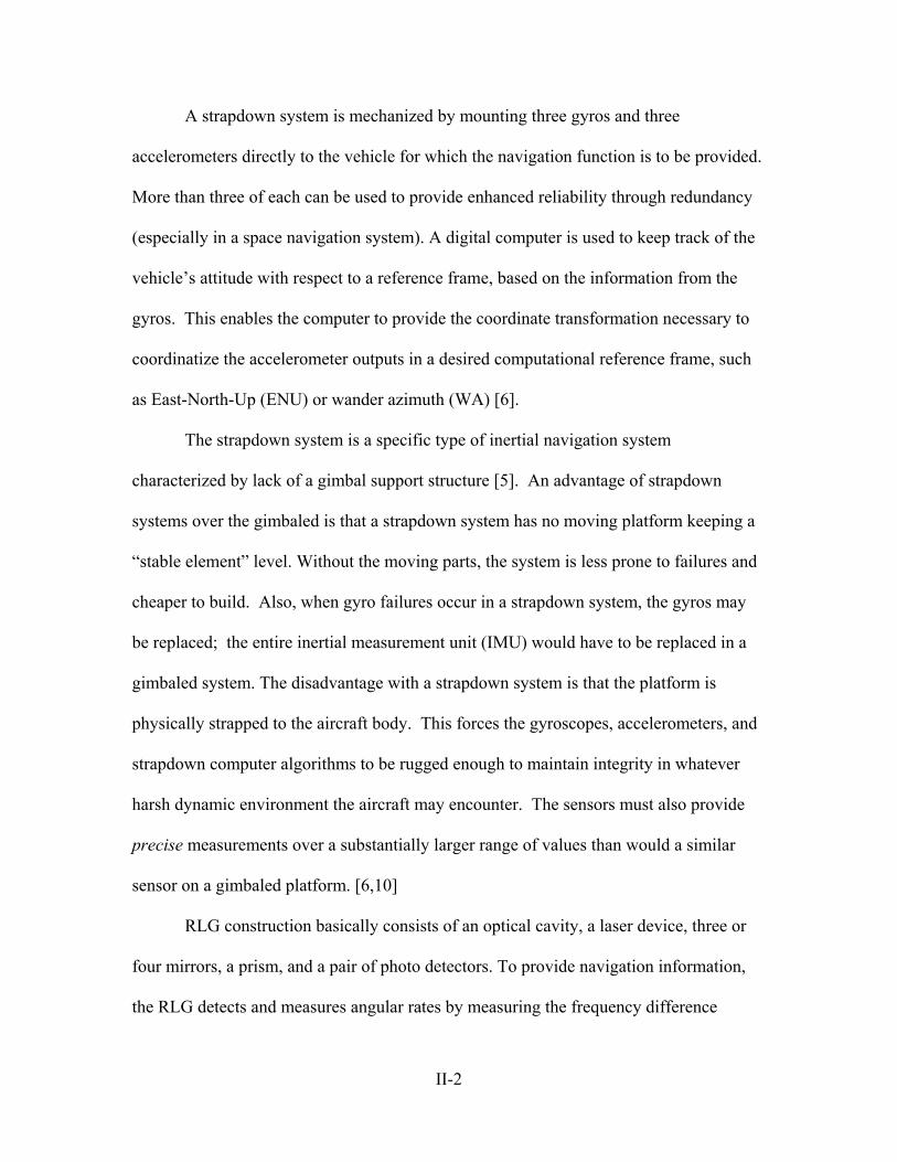
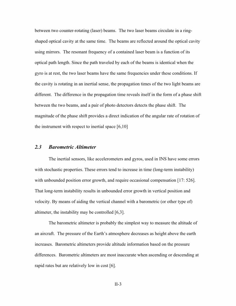
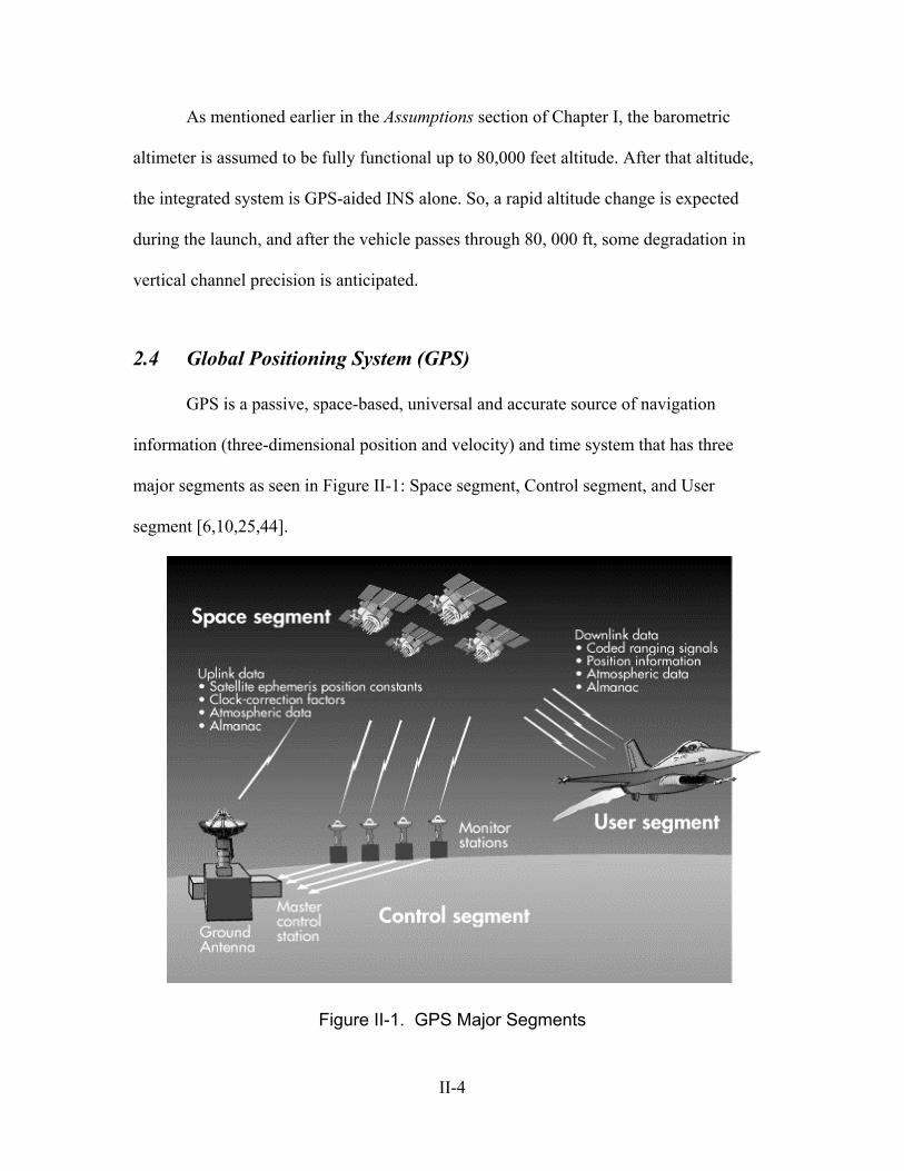
2.4 Global Positioning System (GPS)
GPS is a passive, space-based, universal and accurate source of navigation
information (three-dimensional position and velocity) and time system that has three
major segments as seen in Figure II-1: Space segment, Control segment, and User
segment [6,10,25,44].
Figure II-1. GPS Major Segments
II-4
2.4.1 GPS Space Segment
The GPS Space Segment is composed of 24 or more active satellites in six orbital
planes. See Figure II-2. The satellites operate in nearly 20,200 km (10,900 NM) orbits at
an inclination angle of 55 degrees and with ~ 12-hour period. The spacing of satellites in
orbit is arranged so that a minimum of five satellites (more likely 6-8 satellites) will be in
view to users worldwide, with a position dilution of precision (PDOP) of six or less. One
of the main properties of GPS is the achievable precision, which depends not only on the
accuracy of the pseudorange measurements but also on the geometry of the transmitter
and the receiver. The accuracy of measurements can be transformed by the geometry
from a pseudorange accuracy into a positioning accuracy. This influence is described by
the Dilution of Precision (DOP) factors. Appropriate significance is given to the field of
view of the GPS satellites [1, 42]. PDOP is a measure of the error contributed by the
geometric relationships of the GPS satellites as seen by the GPS receiver [9]. PDOP is
mathematically defined as:
2 2 2x y zPDOP ( )σ σ σ= + + (2.1)
where are the variances of the x, y, and z pseudorange measurement-
based position error, respectively. A definition for pseudorange measurement is given in
Section 2.4.3. Each satellite transmits on two L band frequencies, L1 (1575.42 MHz) and
L2 (1227.6 MHz). L1 carries a precise (P) code and a coarse/acquisition (C/A) code. L2
carries only the P code. A navigation data message containing the important information
about each satellite is overlaid on these codes. The same navigation data message is
carried on both frequencies [10,34].
222 and , zyx σσσ
II-5
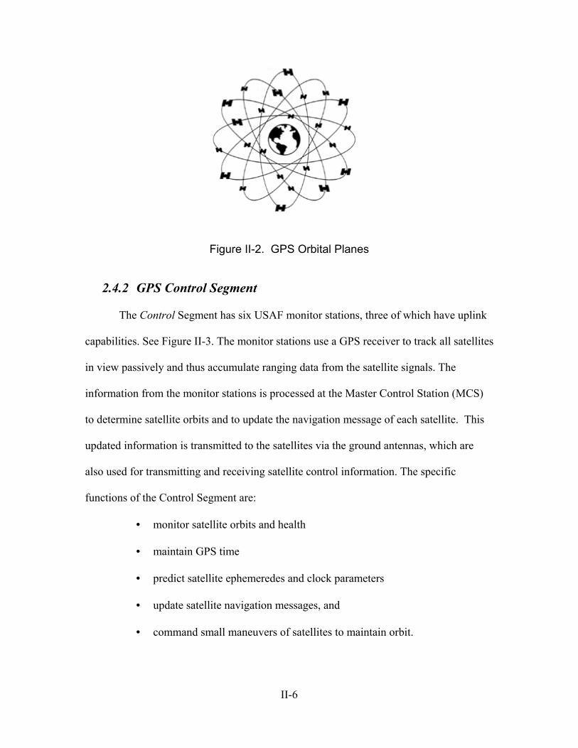
Figure II-2. GPS Orbital Planes
2.4.2 GPS Control Segment
The Control Segment has six USAF monitor stations, three of which have uplink
capabilities. See Figure II-3. The monitor stations use a GPS receiver to track all satellites
in view passively and thus accumulate ranging data from the satellite signals. The
information from the monitor stations is processed at the Master Control Station (MCS)
to determine satellite orbits and to update the navigation message of each satellite. This
updated information is transmitted to the satellites via the ground antennas, which are
also used for transmitting and receiving satellite control information. The specific
functions of the Control Segment are:
• monitor satellite orbits and health
• maintain GPS time
• predict satellite ephemeredes and clock parameters
• update satellite navigation messages, and
• command small maneuvers of satellites to maintain orbit.
II-6
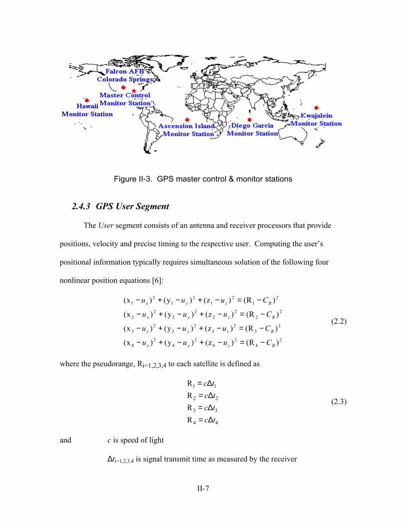
Figure II-3. GPS master control & monitor stations
2.4.3 GPS User Segment
The User segment consists of an antenna and receiver processors that provide
positions, velocity and precise timing to the respective user. Computing the user’s
positional information typically requires simultaneous solution of the following four
nonlinear position equations [6]:
(2.2)
24
24
24
24
23
23
23
23
22
22
22
22
21
21
21
21
)R()z()y()x(
)R()z()y()x(
)R()z()y()x(
)R()z()y()x(
Bzyx
Bzyx
Bzyx
Bzyx
Cuuu
Cuuu
Cuuu
Cuuu
−=−+−+−
−=−+−+−
−=−+−+−
−=−+−+−
where the pseudorange, Ri=1,2,3,4 to each satellite is defined as
(2.3)
1 1
2
3 3
4 4
RRRR
c tc tc tc t
= ∆= ∆= ∆= ∆
2
and c is speed of light
∆ti=1,2,3,4 is signal transmit time as measured by the receiver
II-7
xi=1,2,3,4, yi=1,2,3,4, zi=1,2,3,4 are respective i-th satellite positions
ux, uy, uz is the user position the GPS user equipment is computing
numerically and recursively
CB is the user clock bias (user equipment solves), as expressed in
equivalent range offset in Equation (2.2).
Normally the user equipment needs to acquire and maintain lock on at least four
satellites in order to compute a 3-D position fix u and u [24] and the clock bias CB.
The GPS pseudorange between the user and each satellite is computed based on
knowledge of time (the master GPS clock) and the unique signal format, which is
broadcast by each satellite. Part of the problem is that the user clock is not identical to
the master clock. Once the four pseudoranges are known, a recursive algorithm is solved
to compute the user’s position [24].
yx ,u z
2.5 Differential GPS (DGPS)
Differential GPS is a method of achieving higher GPS positioning accuracies in a
local area. The basic principle behind DGPS is based on the fact that pseudorange
measurement errors are correlated between two nearby receivers tracking a given
satellite. A single DGPS reference station at a known location can compute a range error
correction for each GPS satellite in view. The error corrections may then be broadcast to
users in the vicinity of the reference receiver. A user can typically improve 3-D
positioning accuracy from 10 meters (horizontal DRMS) for a standard GPS down to the
II-8
0.1-1 meter level by applying the corrections to the signals received [34]. The accuracies
do decrease as the distance between the user and the reference station increases.
Work accomplished by William Negast [33] at AFIT has demonstrated the
effectiveness of using differential corrections to increase GPS precision. He was able to
eliminate the satellite vehicle (SV) clock error from each pseudorange measurement, and
the SV position errors were nearly eliminated. The atmospheric propagation errors can
be almost totally eliminated when the two GPS receivers are within 200 miles of each
other [33]. The work by Negast [33] provided the new DGPS error model used in this
effort. Detailed equations for DGPS and explanations for the errors removed from
standard GPS after the application of DGPS corrections are presented in Section 3.6.2.2
2.6 Reference Frames
A navigation "solution" has significance only if the corresponding frame in which
the solution is expressed is clearly understood [36]. While the preceding statement may
seem obvious, it cannot be overemphasized. Consider that a typical INS "owner’s
manual" defines earth frame, true frame, computer frame, platform frame, sensor frame,
accelerometer frame and the body frame [36,5]. From a student’s perspective this may at
first be overwhelming, but to make matters worse, another INS vendor may well define
every frame mentioned above, such as "earth frame" in an entirely different manner!
Therefore, the frames used in this project and the coordinate transformations will briefly
be discussed.
Two variants of a five-frame set (inertial, earth, geodetic, wander-level, and body)
are implemented in PROFGEN (See Figure II-4). One variant is called Standard
II-9
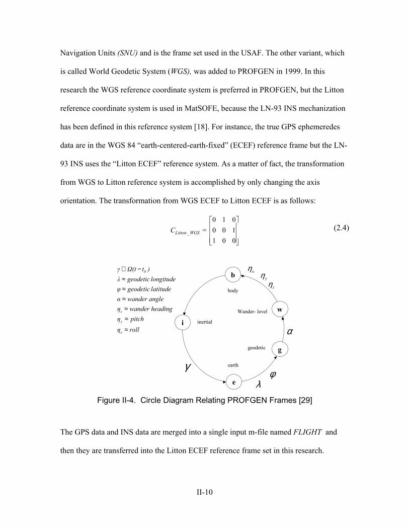
Navigation Units (SNU) and is the frame set used in the USAF. The other variant, which
is called World Geodetic System (WGS), was added to PROFGEN in 1999. In this
research the WGS reference coordinate system is preferred in PROFGEN, but the Litton
reference coordinate system is used in MatSOFE, because the LN-93 INS mechanization
has been defined in this reference system [18]. For instance, the true GPS ephemeredes
data are in the WGS 84 “earth-centered-earth-fixed” (ECEF) reference frame but the LN-
93 INS uses the “Litton ECEF” reference system. As a matter of fact, the transformation
from WGS to Litton reference system is accomplished by only changing the axis
orientation. The transformation from WGS ECEF to Litton ECEF is as follows:
(2.4) 0 1 0
= 0 0 11 0 0
Litton _WGSC
b
w
g
e
xηyη
zη
α
φλ
γ
body
inertial
earth
geodetic
Wander- level
rollη
pitchηheadingwanderη
anglewanderαlatitude geodeticφlongitude geodeticλ
)tΩ(tγ
x
y
z
0
≈
≈≈
≈≈≈
−∝
i
Figure II-4. Circle Diagram Relating PROFGEN Frames [29]
The GPS data and INS data are merged into a single input m-file named FLIGHT and
then they are transferred into the Litton ECEF reference frame set in this research.
II-10
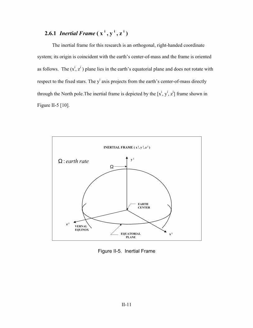
2.6.1 Inertial Frame ( x i , y i , z i )
The inertial frame for this research is an orthogonal, right-handed coordinate
system; its origin is coincident with the earth’s center-of-mass and the frame is oriented
as follows. The (xi, zi ) plane lies in the earth’s equatorial plane and does not rotate with
respect to the fixed stars. The yi axis projects from the earth’s center-of-mass directly
through the North pole.The inertial frame is depicted by the [xi, yi, zi] frame shown in
Figure II-5 [10].
INERTIAL FRAME ( x i, y i, z i )
EQUATORIALPLANE
x i
y i
z i
EARTHCENTER
VERNALEQUINOX
Ωrateearth:Ω
Figure II-5. Inertial Frame
II-11
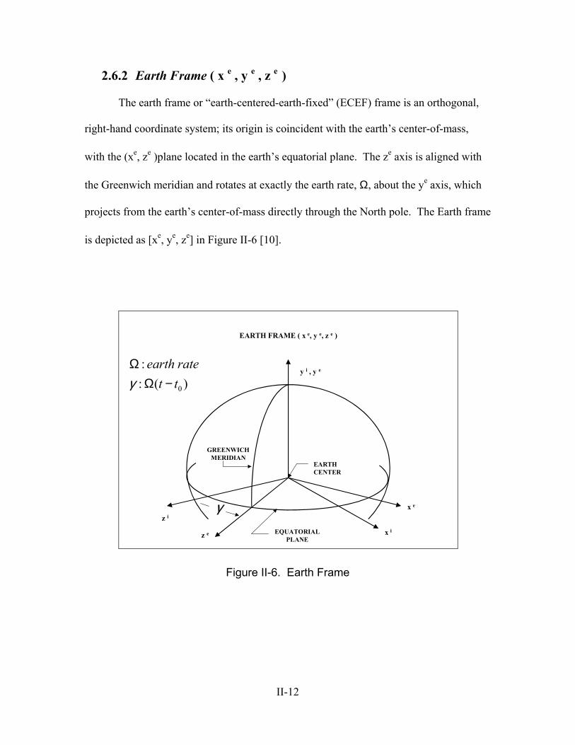
2.6.2 Earth Frame ( x e , y e , z e )
The earth frame or “earth-centered-earth-fixed” (ECEF) frame is an orthogonal,
right-hand coordinate system; its origin is coincident with the earth’s center-of-mass,
with the (xe, ze )plane located in the earth’s equatorial plane. The ze axis is aligned with
the Greenwich meridian and rotates at exactly the earth rate, Ω, about the ye axis, which
projects from the earth’s center-of-mass directly through the North pole. The Earth frame
is depicted as [xe, ye, ze] in Figure II-6 [10].
EQUATORIALPLANE
x i
y i , y e
z i
EARTHCENTER
)(::
0ttrateearth
−ΩΩγ
EARTH FRAME ( x e, y e, z e )
z e
x e
GREENWICHMERIDIAN
γ
Figure II-6. Earth Frame
II-12
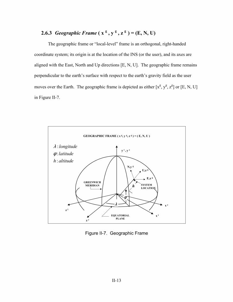
2.6.3 Geographic Frame ( x g , y g , z g ) = (E, N, U)
The geographic frame or “local-level” frame is an orthogonal, right-handed
coordinate system; its origin is at the location of the INS (or the user), and its axes are
aligned with the East, North and Up directions [E, N, U]. The geographic frame remains
perpendicular to the earth’s surface with respect to the earth’s gravity field as the user
moves over the Earth. The geographic frame is depicted as either [xg, yg, zg] or [E, N, U]
in Figure II-7.
GEOGRAPHIC FRAME ( x g, y g, z g ) = ( E, N, U )
EQUATORIALPLANE
x i
y i , y e
z i
z e
x e
GREENWICHMERIDIAN
•
•
SYSTEMLOCATION
N,y gU,z g
E,x g
λ
φ
h
altitudehlatitudelongitude
:::
φλ
Figure II-7. Geographic Frame
II-13
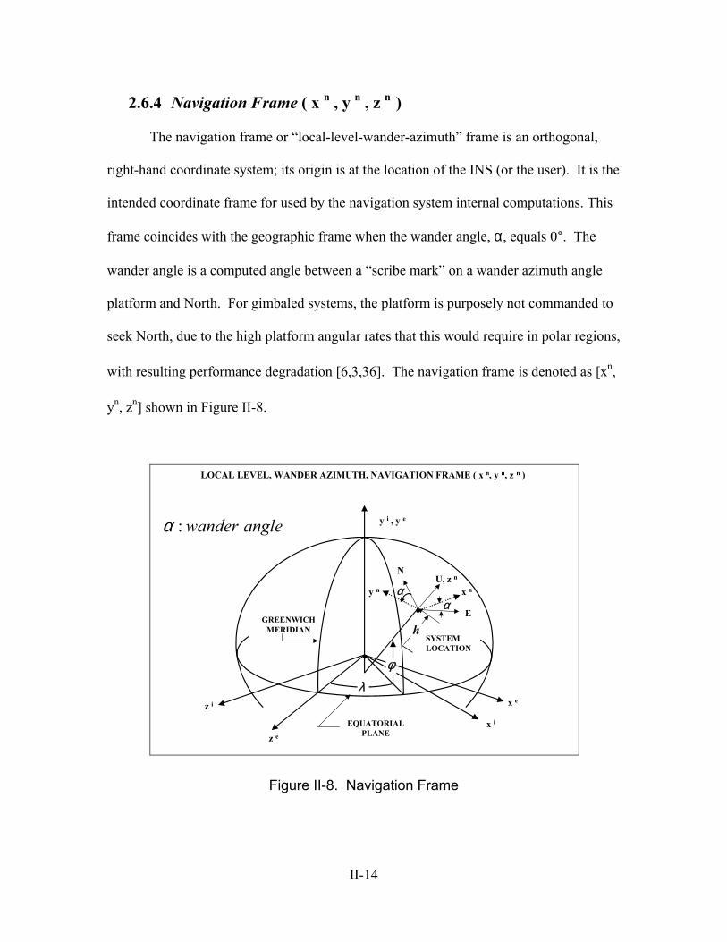
2.6.4 Navigation Frame ( x n , y n , z n )
The navigation frame or “local-level-wander-azimuth” frame is an orthogonal,
right-hand coordinate system; its origin is at the location of the INS (or the user). It is the
intended coordinate frame for used by the navigation system internal computations. This
frame coincides with the geographic frame when the wander angle, α, equals 0°. The
wander angle is a computed angle between a “scribe mark” on a wander azimuth angle
platform and North. For gimbaled systems, the platform is purposely not commanded to
seek North, due to the high platform angular rates that this would require in polar regions,
with resulting performance degradation [6,3,36]. The navigation frame is denoted as [xn,
yn, zn] shown in Figure II-8.
LOCAL LEVEL, WANDER AZIMUTH, NAVIGATION FRAME ( x n, y n, z n )
EQUATORIALPLANE
x i
y i , y e
z i
z e
x e
GREENWICHMERIDIAN
•
•SYSTEMLOCATION
NU, z n
E
x ny n
λ
φ
h
αα
anglewander:α
Figure II-8. Navigation Frame
II-14
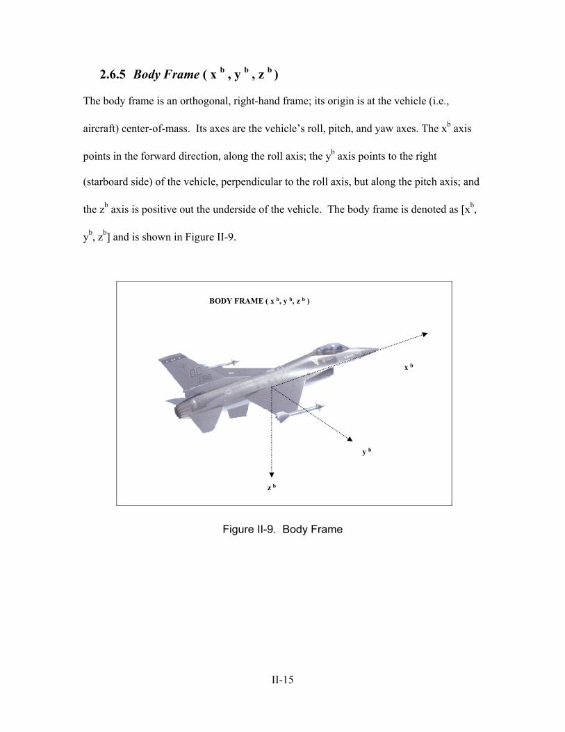
2.6.5 Body Frame ( x b , y b , z b )
The body frame is an orthogonal, right-hand frame; its origin is at the vehicle (i.e.,
aircraft) center-of-mass. Its axes are the vehicle’s roll, pitch, and yaw axes. The xb axis
points in the forward direction, along the roll axis; the yb axis points to the right
(starboard side) of the vehicle, perpendicular to the roll axis, but along the pitch axis; and
the zb axis is positive out the underside of the vehicle. The body frame is denoted as [xb,
yb, zb] and is shown in Figure II-9.
BODY FRAME ( x b, y b, z b )
x b
y b
z b
Figure II-9. Body Frame
II-15
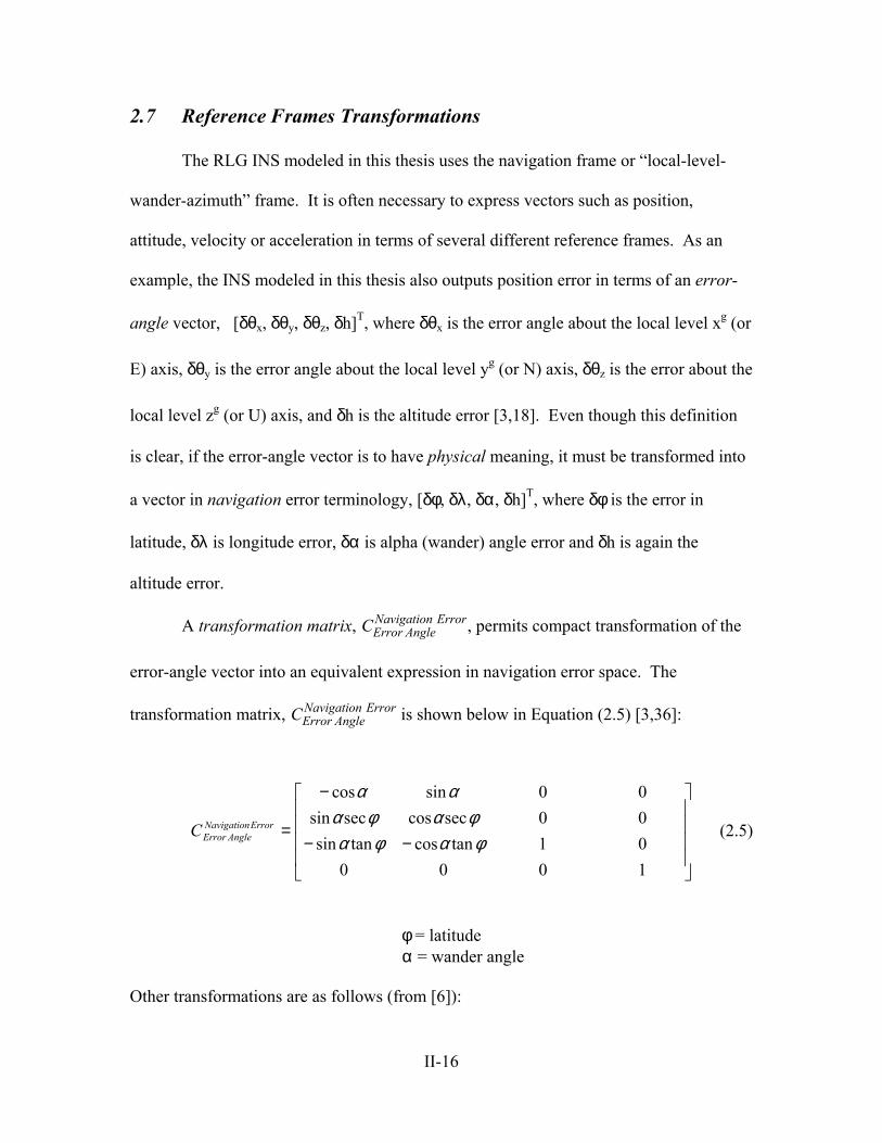
2.7 Reference Frames Transformations
The RLG INS modeled in this thesis uses the navigation frame or “local-level-
wander-azimuth” frame. It is often necessary to express vectors such as position,
attitude, velocity or acceleration in terms of several different reference frames. As an
example, the INS modeled in this thesis also outputs position error in terms of an error-
angle vector, [δθx, δθy, δθz, δh]T, where δθx is the error angle about the local level xg (or
E) axis, δθy is the error angle about the local level yg (or N) axis, δθz is the error about the
local level zg (or U) axis, and δh is the altitude error [3,18]. Even though this definition
is clear, if the error-angle vector is to have physical meaning, it must be transformed into
a vector in navigation error terminology, [δφ, δλ, δα, δh]T, where δφ is the error in
latitude, δλ is longitude error, δα is alpha (wander) angle error and δh is again the
altitude error.
A transformation matrix, CError AngleNavigation Error, permits compact transformation of the
error-angle vector into an equivalent expression in navigation error space. The
transformation matrix, CError AngleNavigation Error is shown below in Equation (2.5) [3,36]:
(2.5)
−−
−
=
100001tancostansin00seccossecsin00sincos
φαφαφαφα
αα
ErrorNavigationAngleErrorC
φ = latitude α = wander angle
Other transformations are as follows (from [6]):
II-16
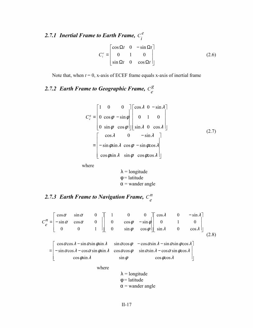
2.7.1 Inertial Frame to Earth Frame, C ei
(2.6)
ΩΩ
Ω−Ω=
tt
ttC e
i
cos0sin010
sin0cos
Note that, when t = 0, x-axis of ECEF frame equals x-axis of inertial frame
2.7.2 Earth Frame to Geographic Frame, geC
(2.7)
−−
−
=
−
−=
λφφλφ
λφφλφ
λλλλ
λλ
φφ
φφ
coscossinsincos
cossincossinsin
sin0cos
cos0sin
010
sin0cos
cossin0
sincos0
001geC
where λ = longitude
φ = latitude α = wander angle
2.7.3 Earth Frame to Navigation Frame, neC
−−−−−−
=
−
−
−=
λφφλφλφαλαφαλφαλαλφαλαφαλφαλα
λλ
λλ
φφφφαα
αα
coscossinsincoscossincossinsincoscossinsincoscossincossinsinsincoscossinsinsinsincoscos
cos0sin010
sin0cos
cossin0sincos0001
1000cossin0sincos
neC
(2.8)
where λ = longitude
φ = latitude α = wander angle
II-17
2.7.4 Geographic Frame to Navigation Frame,C ng
(2.9)
−=
1000cossin0sincos
αααα
ngC
where
α = wander angle
2.7.5 Geographic Frame to Body Frame, bgC
−+−−−+=
−
−
−
−=
θρψρψθρψρψθρθρψρψθρψρψθρ
θψθψθ
ψψψψ
θθ
θθ
ρρρρ
coscossinsincossincoscossinsinsincoscossinsincoscossinsincoscossinsinsin
sincoscossincos
100001010
1000cossin0sincos
cos0sin010
sin0cos
cossin0sincos0
001bgC
(2.10)
where
ρ = roll θ = pitch
ψ = geographic heading
Actually, the rightmost 3x3 matrix of the transformation first transforms from ENU
orientation to NED, then the Navigation-to-Body transformation is accomplished.
bCg
II-18
2.7.6 Navigation Frame to Body Frame, bnC
−+−−−+=
−
−
−
−=
θρψρψθρψρψθρθρψρψθρψρψθρ
θψθψθ
ψψψψ
θθ
θθ
ρρρρ
coscossinsincossincoscossinsinsincoscossinsincoscossinsincoscossinsinsin
sincoscossincos
100001010
1000cossin0sincos
cos0sin010
sin0cos
cossin0sincos0
001
PPPP
PPPP
PP
PP
PPbnC
(2.11)
where
ρ = roll
θ = pitch ψ P = platform heading ( Pψ ψ α= + )
2.8 Kalman Filter Theory
2.8.1 What is a Kalman Filter?
A Kalman filter is simply an optimal recursive data processing algorithm [20] that
can be shown to be optimal by essentially any standard, given the appropriateness of
several underlying assumptions. These assumptions are that the system in question can
be adequately modeled as linear with white, Gaussian system and measurement noises.
One aspect of the word "optimal" is that the Kalman filter can incorporate all
information (measurements) provided to it [20]. It processes all available measurements,
regardless of their precision, to estimate the current value of the variables of interest with
use of (from [20]):
• Knowledge of the system dynamics and measurement device
characteristics.
II-19
• The statistical description of the system noises, measurement errors and
uncertainty in the dynamics models.
• Any available information about initial conditions of the variables of
interest.
For example, to determine the velocity of an aircraft, one could use a Doppler
radar, or the velocity indications from an inertial navigation system, or the pitot and static
pressure and relative wind information in the air data system. Rather than ignore any of
these outputs, a Kalman filter could be built to combine all this data and knowledge of
the various systems’ dynamics and sensor attributes to generate an overall best estimate
of velocity. Another way a Kalman filter is optimal is that it obtains the best estimate of
desired quantities from data provided by a noisy environment. Here the word “optimal”
means that the Kalman filter minimizes mean squared errors and is optimal with respect
to essentially all other criteria, and it does so recursively. The word recursive means that,
unlike certain data processing concepts, the Kalman filter doesn't require all previous data
to be kept in storage and reprocessed every time new measurements are taken.
To see how a Kalman filter works, a simple example taken directly from [20] will
be presented. It is included here because it helped the author understand the concept of a
Kalman Filter in his AFIT studies. Also, the credit for the development of large portions
of this section belongs to Gray [10] and Britton [6].
2.8.2 Kalman Filter Example
Suppose that you are lost at sea during the night and have no idea at all of your
location. So you take a star sighting to establish your position (for the sake of simplicity,
II-20
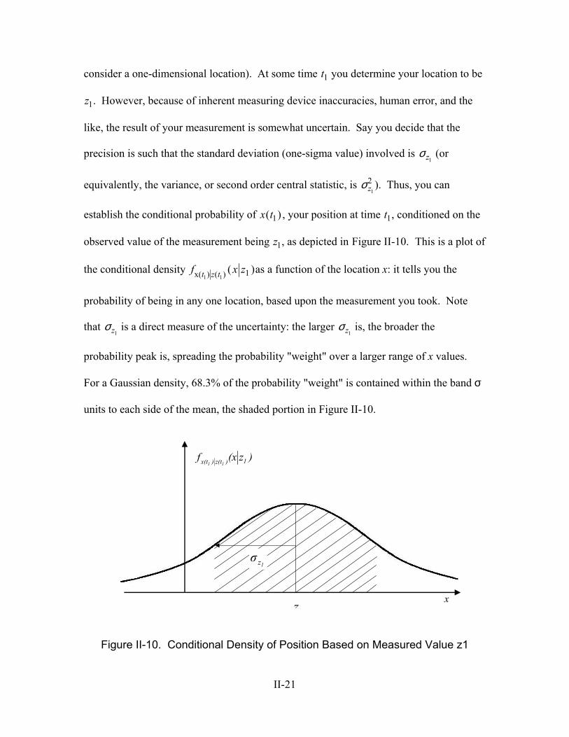
consider a one-dimensional location). At some time t you determine your location to be
. However, because of inherent measuring device inaccuracies, human error, and the
like, the result of your measurement is somewhat uncertain. Say you decide that the
precision is such that the standard deviation (one-sigma value) involved is
1
z1
σz1 (or
equivalently, the variance, or second order central statistic, is ). Thus, you can
establish the conditional probability of
σz1
2
x t( )1
1
, your position at time t , conditioned on the
observed value of the measurement being z , as depicted in Figure II-10. This is a plot of
the conditional density
1
f xt z tx( ) ( ) (1 1 1z )as a function of the location x: it tells you the
probability of being in any one location, based upon the measurement you took. Note
that σz1 is a direct measure of the uncertainty: the larger σz1
is, the broader the
probability peak is, spreading the probability "weight" over a larger range of x values.
For a Gaussian density, 68.3% of the probability "weight" is contained within the band σ
units to each side of the mean, the shaded portion in Figure II-10.
)z(xf 1)z(t)x(t 11
zx
1zσ
Figure II-10. Conditional Density of Position Based on Measured Value z1
II-21
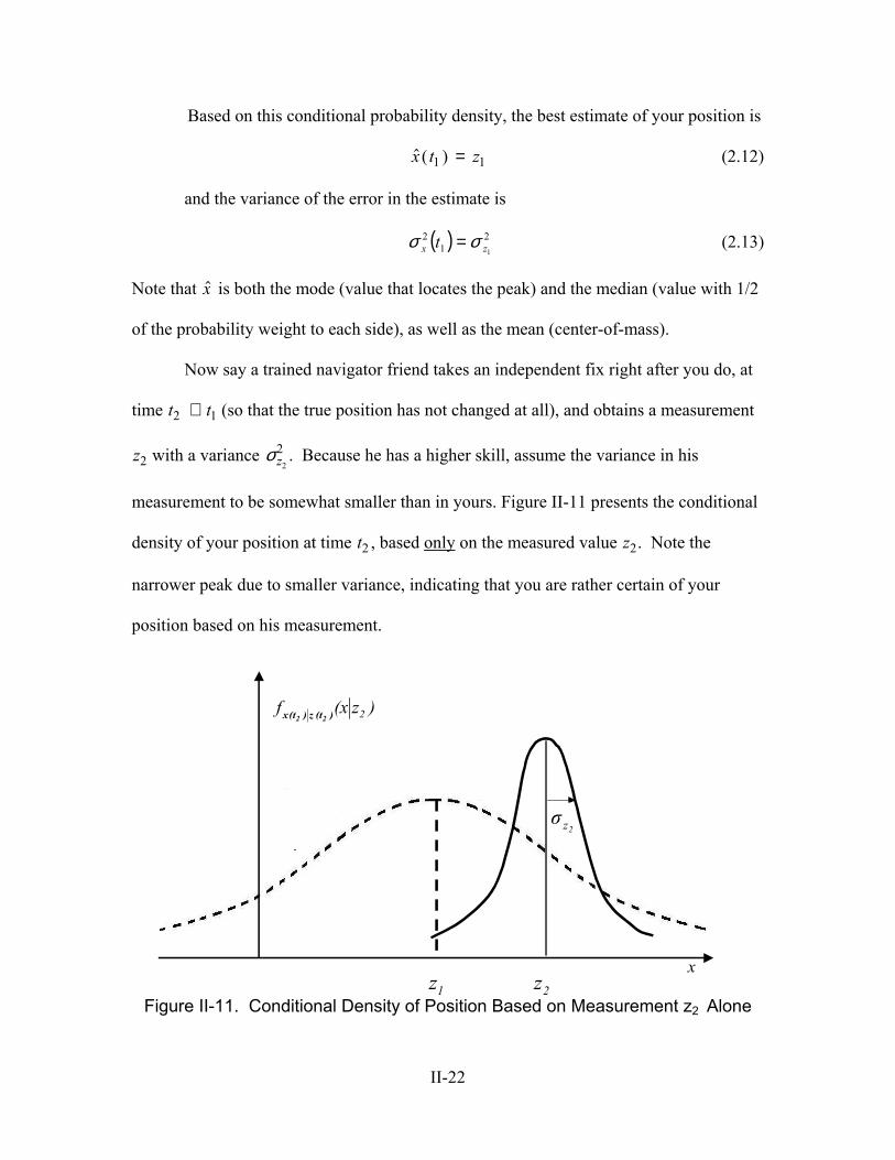
Based on this conditional probability density, the best estimate of your position is
( )x t1 1= z (2.12)
and the variance of the error in the estimate is
22zx σσ (2.13) ( )1 1
t =
Note that x is both the mode (value that locates the peak) and the median (value with 1/2
of the probability weight to each side), as well as the mean (center-of-mass).
Now say a trained navigator friend takes an independent fix right after you do, at
time t (so that the true position has not changed at all), and obtains a measurement
with a variance . Because he has a higher skill, assume the variance in his
measurement to be somewhat smaller than in yours. Figure II-11 presents the conditional
density of your position at time t , based
t12 ≅
z2 σz2
2
2 only on the measured value z . Note the
narrower peak due to smaller variance, indicating that you are rather certain of your
position based on his measurement.
2
)z(xf 2)(tz)(tx 22
1zx
2z
2zσ
Figure II-11. Conditional Density of Position Based on Measurement z2 Alone
II-22
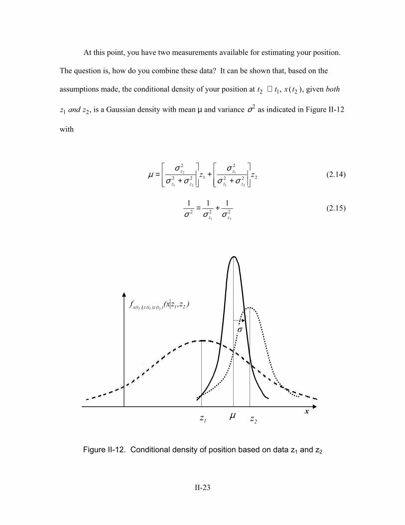
At this point, you have two measurements available for estimating your position.
The question is, how do you combine these data? It can be shown that, based on the
assumptions made, the conditional density of your position at t t , 2 1≅ x t( 2 ), given both
and z , is a Gaussian density with mean µ and variance z1 2 σ2 as indicated in Figure II-12
with
222
2
122
2
21
1
21
2 zzzz
z
zz
z
++
+=
σσσ
σσσ
µ (2.14)
22221
111
zz σσσ+= (2.15)
1zx
2z
)z,z(xf 21)(t)z(tz)(tx 212
σ
µ
Figure II-12. Conditional density of position based on data z1 and z2
II-23
Note that, from (2.15), σ is less than either σz1 or σz2
, which is to say that the
uncertainty in your estimate of position has been decreased by combining the two pieces
of information.
Given this density, the best estimate is
( )x t2 = µ (2.16)
with an associated error variance σ2. It is the mode, the median and the mean (or, since
it is the mean of a conditional density, it is also termed the conditional mean).
Furthermore, it is also the maximum likelihood estimate, the weighted least squares
estimate, and the linear unbiased estimate with variance that is less than that of any other
linear unbiased estimate. In other words, it is the "best" you can do according to just
about any reasonable criterion.
After some study, the form of µ given in (2.14) makes good sense. If σz1 were
equal to σz2, which is to say you think the measurements are of equal precision, the
equation says the optimal estimate of position is simply the average of the two
measurements, as would be expected. On the other hand, if σz1 were larger than σz2
,
which is to say that the uncertainty involved in the measurement z is greater than that of
, then the equation dictates "weighting" z more heavily than z . Finally, the variance
of the estimate is less than
1
1z2 2
σz1 even if σz2
is very large: even poor quality data provides
some information, and should thus increase the precision of the filter output.
The equation for ( )x t2 can be written as
2 1
1 2 1 2
2 2
2 12 2 2 2ˆ( ) z z
z z z z2x t z
σ σσ σ σ σ
= + + +
z (2.17)
II-24
or equivalently as:
][)(ˆ 1222
2
1221
1 zzztxzz
z −
++=
σσσ
(2.18)
or, in final form that is actually used in Kalman filter implementations (noting that
( )x t z1 1= ),
2 1 2 2( ) ( ) ( )[ ( )]ˆ ˆ ˆ 1x t x t K t z - x t= + (2.19)
where
K t z
z z( )2
2
21
1 2
=+
σσ σ2
)
(2.20)
These equations say the optimal estimate at t , 2 (x t2 , is equal to the best
prediction of its value before z is taken, 2 ( )x t1 , plus a correction term of an optimal
weighting value times the residual difference between z and the best prediction of its
value before it is actually taken,
2
( )x t1 . It is worthwhile to understand this "predictor-
corrector" structure of the filter. Based on all previous information, a prediction of the
value that the desired variables and measurement will have at the next measurement time
is made. Then, when the next measurement is taken, the difference between it and its
predicted value is used to "correct" the prediction of the desired variables.
Using the K t( 2 ) in Equation (2.20), the variance equation given by (2.15) can be
rewritten as
σ σ σx x xt t K t22
21 2
21( ) ( ) ( ) (= − t )
)
(2.21)
Note that the values of (x t2 and embody all the information in the Gaussian
density
σ x t2
22( )
f x zx t z t z t( ( ), ( ) )2 1 2 2z( ,1 . Stated differently, by propagating these two variables,
II-25
the conditional density of your position at time t , given z and z , is completely
specified.
2
( )t
)t
1
( )G+
2
)t
) =
Thus we have solved the (static) estimation problem example from [20]. This will
be of vital importance to the practicality of filter implementation. The filter is plain and
simple, “just a computer program in a central processor [20].” If the reader needs a
further example detailing dynamics and propagations, see [20].
2.8.3 Linear Kalman Filter
Whenever possible, a system will be modeled as a set of linear differential
equations of the form [20]:
( ) ( ) ( ) ( ) (x F x B u wt t t t t= + (2.22)
where:
x = "state" vector (n-dimensional)
F = homogenous state dynamics matrix (n x n)
B = control input matrix (n x r)
u = deterministic control input vector ( r-dimensional)
G = driving noise input matrix (n x s)
w = white Gaussian driving noise vector (s-dimensional)
Because the deterministic control term B u is zero in this research, it will be
ignored hereafter. The expected value (i.e. mean), of the white Gaussian driving noise
vector, w(t) is:
( ) (t
E (tw (2.23) 0
II-26
and the noise strength is Q(t):
TE ( t ) ( t ) ( t ) ( )+ =τ δw w Q τ (2.24)
where δ( )⋅ is the Dirac delta function.
While Equation (2.22) is written in terms of "whole" value state variables, the
models used in the thesis are those of error states. This choice of state variable results in
simpler dynamics equations [5], and (2.22) may be rewritten as [20]:
(2.25) ( ) ( ) ( ) ( ) ( )t t t t= +δx F δx G w t
where x(t) has been replaced by the error state vector δx( )t , and all other quantities retain
their previous definitions. The topic of error states is explored more fully in the section
on extended Kalman filters.
As previously stated, the Kalman filter incorporates sampled-data measurement
information from external measuring devices. Irrespective of the type of measuring
device, the equation which is used to describe linear measurements at sample time it
is of the form [3]:
(2.26) ( ) ( ) ( ) ( )i i it t t= +z H x v it
it
or, in the case of error-state models:
(2.27) ( ) ( ) ( ) ( )i i it t t= +δz H δx v
where, in both cases above, H is the observation matrix, and v is a discrete-time zero-
mean white Gaussian measurement noise vector with covariance given by [20]:
II-27
( )
( ) ( )i i
Ti j
i j
t for t tE t t
j
for t t
== ≠
Rv v
0 (2.28)
The Kalman filter "propagates" the error state and its covariance from the instant
in time immediately following the most recent measurement update, t , to the instant in
time immediately preceding the next measurement update, t , by numerical integration
of the following equations [20]:
i+
i +−
1
(2.29) ˆ ( / ) ( ) ( / )it t t t t=x F x i
( / ) ( ) ( / ) ( / ) ( ) ( ) ( ) ( )P F P P F G Q Gt t t t t t t t t t ti i i
T T= + + (2.30)
The notation for ( / )t tix and associated error covariance P( / )t ti
i
indicate the
best estimate of x and P at time t, based on measurements through time t , and t is in the
interval from to t . Initial conditions are given as it+
1i−
+
ˆ ˆ( ) ( / )i it t+ =x x it
it
)it )it
(2.31)
( ) ( / )i it t+ =P P (2.32)
as provided by the measurement update cycle at time t . The variables t and t
indicate the initial and final times for each integration period, respectively.
i i i +1
After propagation, and are "updated"
(meaning that state estimates are revised, based on new measurement information). The
pivotal element in the update equations for sample time t (rather than time t ) shown
below is the time-varying Kalman filter gain K . The K matrix assigns "weights"
1 1ˆ ˆ( ) ( /i it t−+ +=x x 1 1( ) ( /i it t−
+ +=P P
i
( )ti ( )ti
1i+
II-28
to the "measurement residual" (the residual consists of the difference between the actual
measurement and the filter's prediction of the measurement) based on known
measurement noise statistics and filter-computed state error covariance from the previous
time step. This process is designed to improve the estimate of each element of the state
vector. The update equations are [20]:
1)()()()()()()( −−− += iiT
iiiT
ii ttttttt RHPHHPK (2.33)
)](ˆ)()()(ˆ)(ˆ iiiiii ttttt xHzKxx −+= −+
ti−
)ti−
)ti+
(2.34)
P P (2.35) K H P( ) ( ) ( ) ( ) ( )t t t ti i i i+ −= −
Although the algorithm shown above is generally applicable to any problem
which lends itself to a Kalman filtering solution, it is not necessarily the algorithm which
is used in practice. It is often advantageous to use a form of the algorithm known as the
U-D factorization form [20]. In the U-D algorithm, the filter covariance matrix is not
propagated and updated as a single square array. The U and D matrices below
representing the pre- and post-measurement filter covariances, respectively, are explicitly
computed instead [20]:
P U D U( ) ( ) ( ) (t t ti i i− − −= (2.36)
P U D U( ) ( ) ( ) (t t ti i i
+ + += (2.37)
where the U matrices are upper triangular and unitary (and thus contain ones along the
main diagonal), and the D matrices are simply diagonal [20]. This form offers several
advantages, including numerical stability, improved precision, and guaranteed non-
negativity of the computed covariance's eigenvalues [20]. It is the U-D form of the
II-29
Kalman filter algorithm which is implemented in the MatSOFE software [12] that is used
in this research.
2.8.4 Linearized and Extended Kalman Filter
Not all problems are adequately described with linear systems driven by white
Gaussian noise. In many cases, the most appropriate model is nonlinear. The navigation
problem at hand falls squarely into the nonlinear category (at least for the measurement
model). Fortunately, a relinearized method exists whereby a nonlinear system may be
treated in much the same manner as a linear one for a particular class of problems.
Suppose that the nonlinear system may be described by [21]:
( ) [ ( ), ( ), ] ( ) ( )x f x u G wt t t t t= + t
ti
(2.38)
In this case, the state dynamics vector, f [⋅, ⋅, ⋅], is a nonlinear function of the state vector
, the control input (assumed to be zero in this research), and time t. The white
Gaussian noise is defined exactly as in (2.23) and (2.24), and it still enters the dynamics
model linearly. In addition, the measurement equation may also be a nonlinear function
of the state vector and time [21]:
x( )⋅
z h x v( ) [ ( ), ] ( )t t ti i i= + (2.39)
The noise vector v is again zero-mean, white and Gaussian, entering the measurement
equation linearly, and its covariance is described by (2.28).
Recalling that a system must be linear in order to satisfy the assumptions upon
which a conventional Kalman filter is based, the nonlinear equations (2.38) and (2.39)
must be linearized. The following approach is summarized from [21]:
II-30
1. Assume that a nominal state trajectory, x , may be generated which satisfies n t( )
xn t( )0 0= xn
t t
t
t
(2.40)
and
( ) [ ( ), ( ), ]x f x un nt t= (2.41)
where f [⋅, ⋅, ⋅] is specified in (2.38), and u(t)=0.
2. The “nominal” measurements, which accompany the nominal trajectory, are:
z h xn i n i it t( ) [ ( ), ]= (2.42)
3. The “perturbation” of the state derivative is obtained by subtracting the nominal
trajectory from the original nonlinear equation:
[ ( ) ( )] [ ( ), ( ), ] [ ( ), ( ), ] ( ) ( )x x f x u f x u G wt t t t t t t t tn n− = − + (2.43)
4. The equation above may be approximated to first order by a Taylor series expansion:
δ δ( ) [ ; ( )] ( ) ( ) ( )x F x x G wt t t t tn= + t (2.44)
where δx( )⋅
( )]tn
represents a first-order approximation of the process [ , and
is a matrix of partial derivatives of f with respect to its first argument,
evaluated along the nominal trajectory [21]:
( ) ( )]x x⋅ − ⋅n
F x[ ;t
F x f xx x x
[ ; ( )] [ , ]( )
t t ttn
n=
=∂
∂ (2.45)
5. The perturbation measurement equation is derived in like fashion and is expressed as
[21]:
δ δz H x x v( ) [ ; ( )] ( ) ( )t t t ti i n i= ti+ (2.46)
II-31
where
H xh x
x x x[ ; ( )]
[ , ]( )
t tt
ti n ii
n i=
=∂
∂ (2.47)
With the “error-state” model (2.44)-(2.47) in hand, it is possible to return to the linear
filtering theory. An estimate of the whole-valued quantities of interest is obtained from
[21]:
ˆ ( ) ( )n t= +δx x x t (2.48)
The expression above for the linearized Kalman filter is useful, provided that the
linearization assumption is not violated. However, if the nominal and “true” trajectories
differ by too large an amount, unacceptable errors may result [21]. It is for this reason
that extended Kalman filtering is useful in many cases for which perturbation techniques
alone do not suffice. Extended Kalman filtering allows for relinearizing about newly
declared nominals at each sample time, to enhance the adequacy of the linearization
process, and thus of the resulting filter performance as well [21].
The extended Kalman filter equations are summarized below. The reader is
referred to [21] for details regarding their derivation. The assumed measurement model
equation for an extended Kalman filter development is given by Equation (2.39), where
is once again zero-mean, white and Gaussian, with covariance given by (2.28).
Measurements are incorporated into the extended Kalman filter via the following set of
equations [21]:
v ( )⋅
1)()](ˆ;[)()](ˆ;[)](ˆ;[)()( −−−−−− += iiiT
iiiiiT
ii tttttttttt RxHPxHxHPK (2.49)
]);(ˆ[)()(ˆ)(ˆ iiiiii ttttt −−+ −+= xhzKxx (2.50)
II-32
)()](ˆ;[)()()( −−−+ −= iiiiii tttttt PxHKPP (2.51)
where
)(ˆ],[
)](ˆ;[ −−
==
i
iii t
ttt
xxxxh
xH∂
∂ (2.52)
The state estimate and covariance are propagated from t to t by integrating the
following equations [21]:
i i +1
( / ) [ ( / ), ( ), ]x f x ut t t t t ti i= (2.53)
( / ) [ ; ( / )] ( / ) ( / ) [ ; ( / )] ( ) ( ) ( )P F x P P F x G Q Gt t t t t t t t t t t t t t ti i i iT
iT= + + (2.54)
where
[ ( ), ]ˆ[ ; ( / )]ˆ ( / )
ii
i
t tt t tt t
==
∂∂
f xF xx x x
(2.55)
and the initial conditions are:
ˆ ˆ( / ) ( )i i it t t+=x x (2.56)
P P( / ) (t t ti i i= + ) (2.57)
The equations shown above for the extended Kalman filter are programmed into
the MatSOFE shell [12] for the problem defined by this thesis. It is the fact that the
extended Kalman filter is relinearized about each successive estimate of the state
which “enhances the validity of the assumption that deviations from the reference
(nominal) trajectory are small enough to allow linear perturbation techniques to be
employed” [21].
( )x t
II-33
2.9 Summary
This chapter has presented the basic theory of an RLG-based strapdown INS,
GPS, DGPS, and barometric altimeter. Reference frames and coordinate transformations
used in this thesis have also been defined. A Kalman filter example from [20] was given
and linear, linearized and extended Kalman filter fundamentals were discussed from
[21]. The purpose of this chapter was to provide a flavor of Kalman filtering. Chapter 3
will describe the design methodology and error models of the RLG-based strapdown INS,
GPS, DGPS, and barometric altimeter used in this thesis for MatSOFE simulations. More
information on Kalman filter development and uses may be found in [20,21,22].
II-34
III. Design Methodology and Error Models
3.1 Overview
This chapter describes the set-up of the MatSOFE computer simulation for the
Space Navigation System Model (SNSM) error model. This chapter also describes the
technique used to determine which “real-world” (true) satellite vehicle (SV) ephemeris
data was used during MatSOFE simulation. A brief description on using PROFGEN [52]
to generate a transport aircraft profile and a launch vehicle flight profile will also be
discussed. The Tanker profile is used to validate the simulation tool by comparing results
to previous research results; the next chapter describes the use of PROFGEN to generate
a satellite launch rocket trajectory for this effort. As with Chapter 2, the background
works done by Gray [10] and Britton [6] laid the foundations for large portions of this
chapter. The credit for the development of large portions of this chapter should be given
to them.
3.2 Introduction to MatSOFE
The name "MSOFE" is an acronym meaning "Multimode Simulation for Optimal
Filter Evaluation." MSOFE is a general-purpose, multimode simulation program for
designing integrated systems that employ optimal Kalman filtering techniques and for
evaluating their performance [29]. Its general-purpose construction allows specific user
problems to be simulated more quickly and at less cost than without its use. MSOFE has
been designed to support a wide variety of system simulation and filter evaluation efforts.
It provides two major operating modes:
III-1
1) Monte Carlo simulation: to generate multiple sample time
histories of system truth states, filter states, and filter estimation errors, including
nonlinear effects; usable for linear and extended Kalman filters;
2) Covariance simulation: to generate time histories of the second-
order statistics (covariances) of system truth states, filter states, and filter estimation
errors, under the assumption of linear (or linearized) models.
Monte Carlo and covariance simulation modes of MSOFE are complementary to
one another. The covariance mode can generate filter performance statistics via a single
run, whereas the Monte Carlo mode requires several sample runs (say, 15 or more) to
generate meaningful statistics for a given scenario. However, the covariance mode is
limited to linear (or linearized) systems, whereas the Monte Carlo mode can represent
nonlinear as well as linear dynamic and measurement processes. In addition, the Monte
Carlo mode provides better visibility into the detailed workings of the filter models and
computation processes, and can easily be reduced to a deterministic mode (by
suppressing noise sampling) when required [10,6].
MSOFE has been the primary tool used in the design and evaluation of the
Kalman filters by AFIT students at Wright-Patterson AFB, Ohio. As stated earlier,
MSOFE is restricted to use by U.S. government agencies and their U.S. contractors. As
an international officer, the author is not eligible to use MSOFE in the role of a tool for
Kalman filter evaluation. For that reason the Matlab based [37] “MatSOFE” is used in
this research to conduct navigation performance analysis of a launch vehicle. MatSOFE
was first created by former AFIT student William B. Mosle [27], GE/93D, in 1993 and
modified by Pamela L. Harms [12] in 1995 for Sverdrup Technology, Inc., TEAS Group
III-2
most recently before the author received it. Before the author received it, MatSOFE was
the analysis tool that had been used on the Exploitation of Differential Global Positioning
System (GPS) for Guidance Enhancement (EDGE) Program to conduct a navigation
performance analysis in TEAS group. That received version will be called the EDGE-
version MatSOFE in this thesis.
“MatSOFE is written entirely in Matlab [37] code. Matlab is an interactive system
and programming language for general scientific and technical computation. MatSOFE
has been written as a set of Matlab scripts and functions using m-files. The m-file is a
feature of Matlab used in the MatSOFE tool” [12]. This feature allows the user to execute
sequences of commands that are stored in files with separate names and extension of
“.m”, as in “Matsofe_in.m” which is in fact an m-file in which the filter process strength
(Q) and measurement noise covariance (R) are stated along with all the constants used in
simulation.
MatSOFE is designed only for Monte Carlo simulations. It does not have the
capability of making a covariance analysis. Such a capacity could be added to MatSOFE
performance evaluation as well, but as is discussed clearly earlier, the covariance analysis
is limited to linear (or linearized) systems, whereas the Monte Carlo simulations can
represent nonlinear as well as linear dynamic and measurement processes. Besides that,
the “real world” is itself nonlinear for this application. 15 runs of Monte Carlo
simulations (unless otherwise noted) are made in this research by using MatSOFE.
The latest version MatSOFE is the outcome of a collective effort. Many people
struggled to reflect their knowledge in Matlab and Kalman filtering before it reached
today’s capabilities. At the time of delivery, the EDGE version MatSOFE had 53 m-files,
III-3
containing a 48-state strapdown INS/GPS model, which includes 21 states for INS and 27
states for GPS (with 5 modeled GPS SV errors) along with a 17-state filter model. It had
a limited capability. The GPS orbit model was a fairly simplistic model and was not very
realistic for anything other than extremely short flight trajectories (less than two minutes)
During this research, 21 m-files have been deleted, 18 new m-files have been added, and
almost all others have been modified to be adequate for a realistic launch vehicle
simulation. Currently, MatSOFE has a 69-state (61-state for DGPS) LN-93 INS/GPS
integration truth model, which includes a 39-state reduced order LN-93 INS model and
30-state GPS (22-state for DGPS) error model. The filter model contains 13 states (9
states for Pinson error variables’ definition, 2 states for barometric stabilization, and 2
states for GPS). Unlike the EDGE version, it uses “simulated true GPS data”, and the
U-D factorization algorithm in order to increase the numerical stability in the Kalman
filter.
Similar to MSOFE, MatSOFE permits the user to design integrated systems
through Kalman filtering techniques and provides a reliable evaluation tool for that
purpose. The power of Matlab makes MatSOFE an excellent software tool for “realistic”
implementation of Kalman filter performance evaluation tool analogous to the Fortran-
based MSOFE. One advantage of MatSOFE is that it is capable of making matrix
operations versus the Fortran-based program, MSOFE, which performs scalar operations.
Additional advantages of MatSOFE include access to data, simplicity of programming,
ease to build models, simplicity to obtain outputs, familiarization of AFIT students with
Matlab and relative ease in troubleshooting and debugging. On the other hand, using a
III-4
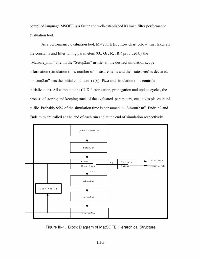
compiled language MSOFE is a faster and well-established Kalman filter performance
evaluation tool.
As a performance evaluation tool, MatSOFE (see flow chart below) first takes all
the constants and filter tuning parameters (Qs, Qf , Rs , Rf ) provided by the
“Matsofe_in.m” file. In the “Setup2.m” m-file, all the desired simulation scope
information (simulation time, number of measurements and their rates, etc) is declared.
“Initrun2.m” sets the initial conditions (x(t0), P(t0) and simulation time controls
initialization). All computations (U-D factorization, propagation and update cycles, the
process of storing and keeping track of the evaluated parameters, etc., takes places in this
m.file. Probably 95% of the simulation time is consumed in “Simrun2.m”. Endrun2 and
Endsim.m are called at t he end of each run and at the end of simulation respectively.
C le a r V a r ia b le s
S e tu p 2 .m
I n i tru n 2 .m
S im ru n 2 .m
E n d ru n 2 .m
W h ile
IR u n < R u n s
E n d s im .m
I R u n = IR u n + 1
O u tp u t
P r in t P lo ts
S a v e to F ileN o
Y e s
Figure III-1. Block Diagram of MatSOFE Hierarchical Structure
III-5
3.3 Introduction to PROFGEN
PROFGEN calculates kinematic data for a simulated air vehicle (aircraft, missile,
rocket) moving in free space over the earth. Kinematics is concerned with space and time,
and with the time rate of change of quantities that describe the geometry of motion.
Kinematic data include translational variables like position and velocity, and rotational
variables like angle and angular rate, which portray the aircraft’s dynamic state [29].
PROFGEN models the aircraft as a point mass body. There are no actuators, no
control surfaces, no aerodynamics, and no propulsion system. Position is given as
(geographic) latitude, longitude and altitude. Velocity with respect to earth is
coordinatized and presented in a local-vertical frame. Acceleration consists of velocity
rates-of-change summed with Coriolis effects and gravity. Attitude consists of roll, pitch
and yaw: the Euler angles [6]. PROFGEN tool utilities are stand-alone interactive
programs that (mostly) prompt for their inputs. To use PROFGEN, one must supply an
input file that specifies the desired trajectory.
PROFGEN builds a complete trajectory from a sequence of flight segments, one
segment following another in time. The final values of the variables for segment “k”
become the initial values for the segment “k+1”, thereby maintaining continuous-time
histories for all output quantities. Each flight segment executes one “maneuver” at a time,
with six kinds of maneuvers being possible: straight flights, rolls, vertical turns,
horizontal turns, jinking and free fall. Since it cannot do several maneuvers
simultaneously, PROFGEN cannot be made to perform intricate actions like Immelmanns
or barrel rolls. This will be limiting for some applications [29]. Flight segments should
not exceed 53.
III-6
PROFGEN’s kinematic computations track the motion of the aircraft in six
degrees of freedom (6-DOF). The vehicle may move anywhere in 3-space and may
achieve any attitude except vertical flight. The vector variables can be output in any of
four coordinate frames (inertial, earth, wander-level, body). Direction cosine matrices
between pairs of frames can also be output. See Table III-1 for PROFGEN flight profile
outputs.
PROFGEN has been used to create trajectories for a variety of aircraft including
bombers, fighters, transporters, and helicopters. But it is also able to produce trajectories
other than aircraft. For example, it has been used to simulate missile flights, bombs in
free fall, satellites in Earth orbit, and busses driving highways.
For this study the latest version of PROFGEN (Version 8.1) is used to generate
trajectories. In order to validate MatSOFE as a reliable Kalman filtering performance
evaluation tool, the work accomplished by Gray [10], Britton [6], and Mosle [27] are
regenerated in the MatSOFE environment. To do this job, the KC-135 Tanker aircraft
flight profile of these previous research efforts is generated in PROFGEN by using the
provided PROF_IN code in Gray’s thesis. After MatSOFE is validated, at the second
stage, the Atlas IIAS launch profile is generated in PROFGEN. The Atlas flight profile
has 8 flight segments. The segments for the “Tanker” flight profile used in this thesis are
shown in Table III-2. The parameters shown in Table III-2 are computed by the author
taking the actual flight characteristics into account. Appendix C shows the Fortran-
based PROF_IN file for the Atlas launch vehicle and Figure III-2 shows the plot of 2-
dimensional PROFGEN-generated rocket profile.
III-7
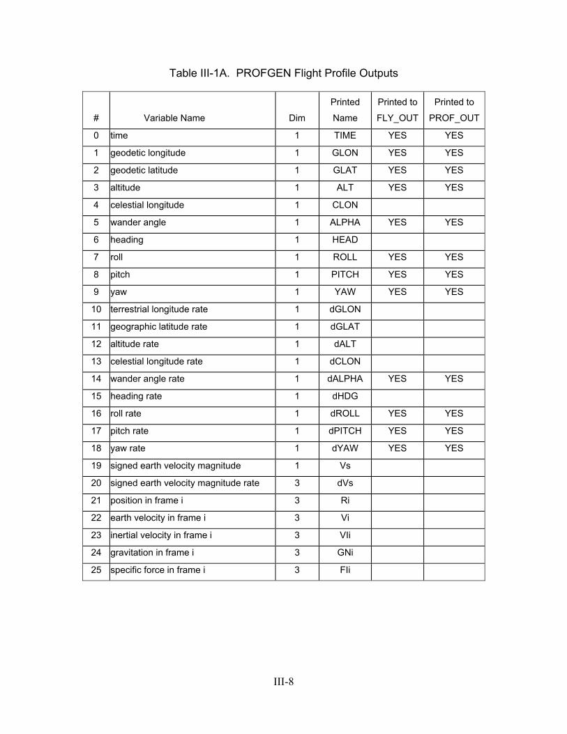
Table III-1A. PROFGEN Flight Profile Outputs
# Variable Name Dim
Printed
Name
Printed to
FLY_OUT
Printed to
PROF_OUT
0 time 1 TIME YES YES
1 geodetic longitude 1 GLON YES YES
2 geodetic latitude 1 GLAT YES YES
3 altitude 1 ALT YES YES
4 celestial longitude 1 CLON
5 wander angle 1 ALPHA YES YES
6 heading 1 HEAD
7 roll 1 ROLL YES YES
8 pitch 1 PITCH YES YES
9 yaw 1 YAW YES YES
10 terrestrial longitude rate 1 dGLON
11 geographic latitude rate 1 dGLAT
12 altitude rate 1 dALT
13 celestial longitude rate 1 dCLON
14 wander angle rate 1 dALPHA YES YES
15 heading rate 1 dHDG
16 roll rate 1 dROLL YES YES
17 pitch rate 1 dPITCH YES YES
18 yaw rate 1 dYAW YES YES
19 signed earth velocity magnitude 1 Vs
20 signed earth velocity magnitude rate 3 dVs
21 position in frame i 3 Ri
22 earth velocity in frame i 3 Vi
23 inertial velocity in frame i 3 VIi
24 gravitation in frame i 3 GNi
25 specific force in frame i 3 FIi
III-8
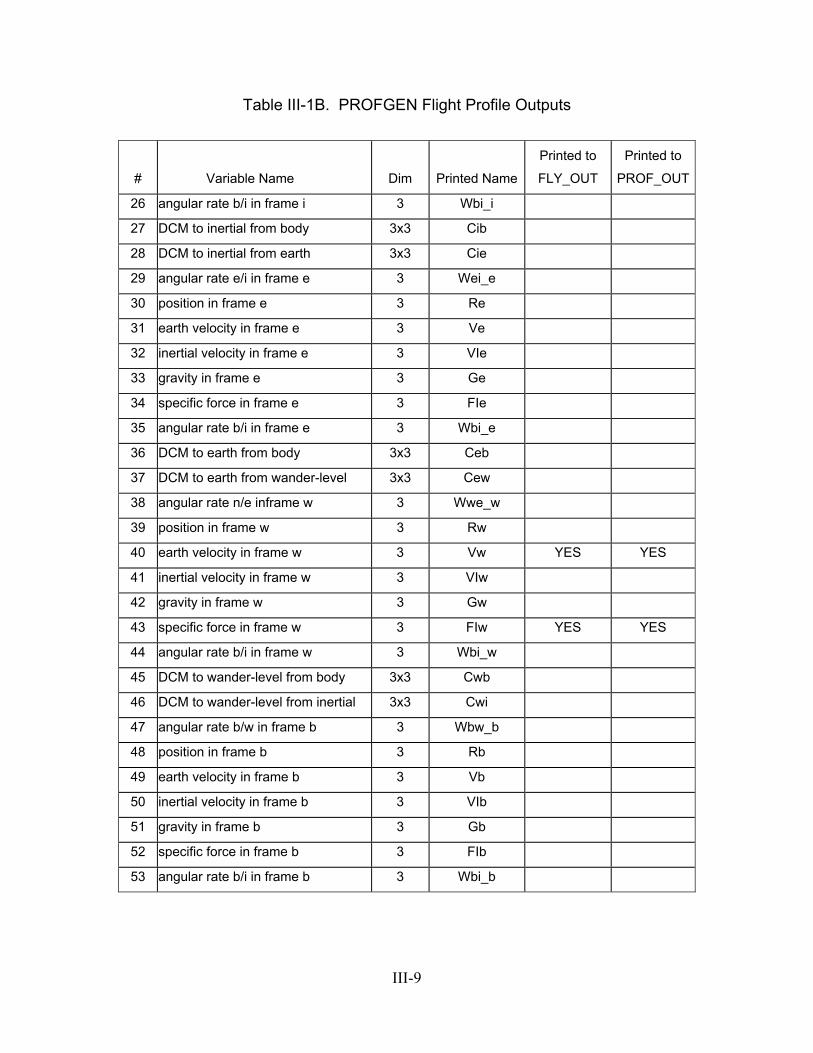
Table III-1B. PROFGEN Flight Profile Outputs
# Variable Name Dim Printed Name
Printed to
FLY_OUT
Printed to
PROF_OUT
26 angular rate b/i in frame i 3 Wbi_i
27 DCM to inertial from body 3x3 Cib
28 DCM to inertial from earth 3x3 Cie
29 angular rate e/i in frame e 3 Wei_e
30 position in frame e 3 Re
31 earth velocity in frame e 3 Ve
32 inertial velocity in frame e 3 VIe
33 gravity in frame e 3 Ge
34 specific force in frame e 3 FIe
35 angular rate b/i in frame e 3 Wbi_e
36 DCM to earth from body 3x3 Ceb
37 DCM to earth from wander-level 3x3 Cew
38 angular rate n/e inframe w 3 Wwe_w
39 position in frame w 3 Rw
40 earth velocity in frame w 3 Vw YES YES
41 inertial velocity in frame w 3 VIw
42 gravity in frame w 3 Gw
43 specific force in frame w 3 FIw YES YES
44 angular rate b/i in frame w 3 Wbi_w
45 DCM to wander-level from body 3x3 Cwb
46 DCM to wander-level from inertial 3x3 Cwi
47 angular rate b/w in frame b 3 Wbw_b
48 position in frame b 3 Rb
49 earth velocity in frame b 3 Vb
50 inertial velocity in frame b 3 VIb
51 gravity in frame b 3 Gb
52 specific force in frame b 3 FIb
53 angular rate b/i in frame b 3 Wbi_b
III-9
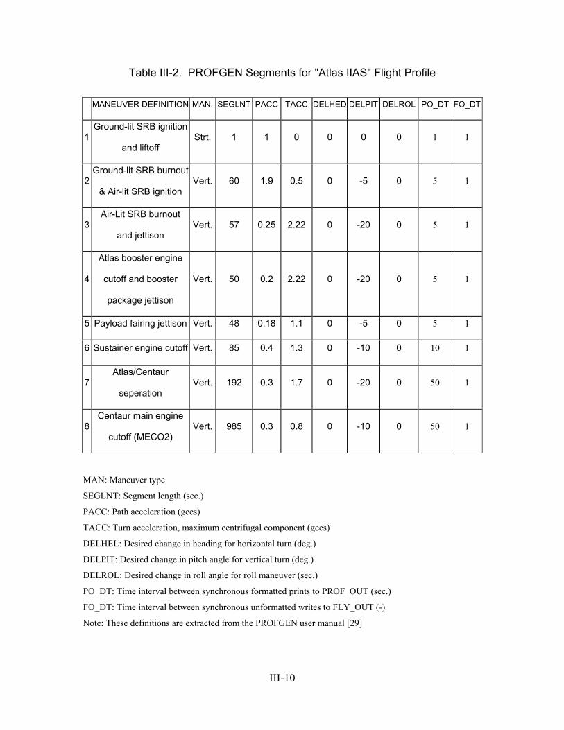
Table III-2. PROFGEN Segments for "Atlas IIAS" Flight Profile
MANEUVER DEFINITION MAN. SEGLNT PACC TACC DELHED DELPIT DELROL PO_DT FO_DT
1Ground-lit SRB ignition
and liftoff Strt. 1 1 0 0 0 0 1 1
2Ground-lit SRB burnout
& Air-lit SRB ignition Vert. 60 1.9 0.5 0 -5 0 5 1
3Air-Lit SRB burnout
and jettison Vert. 57 0.25 2.22 0 -20 0 5 1
4
Atlas booster engine
cutoff and booster
package jettison
Vert. 50 0.2 2.22 0 -20 0 5 1
5 Payload fairing jettison Vert. 48 0.18 1.1 0 -5 0 5 1
6 Sustainer engine cutoff Vert. 85 0.4 1.3 0 -10 0 10 1
7Atlas/Centaur
seperation Vert. 192 0.3 1.7 0 -20 0 50 1
8Centaur main engine
cutoff (MECO2) Vert. 985 0.3 0.8 0 -10 0 50 1
MAN: Maneuver type
SEGLNT: Segment length (sec.)
PACC: Path acceleration (gees)
TACC: Turn acceleration, maximum centrifugal component (gees)
DELHEL: Desired change in heading for horizontal turn (deg.)
DELPIT: Desired change in pitch angle for vertical turn (deg.)
DELROL: Desired change in roll angle for roll maneuver (sec.)
PO_DT: Time interval between synchronous formatted prints to PROF_OUT (sec.)
FO_DT: Time interval between synchronous unformatted writes to FLY_OUT (-)
Note: These definitions are extracted from the PROFGEN user manual [29]
III-10
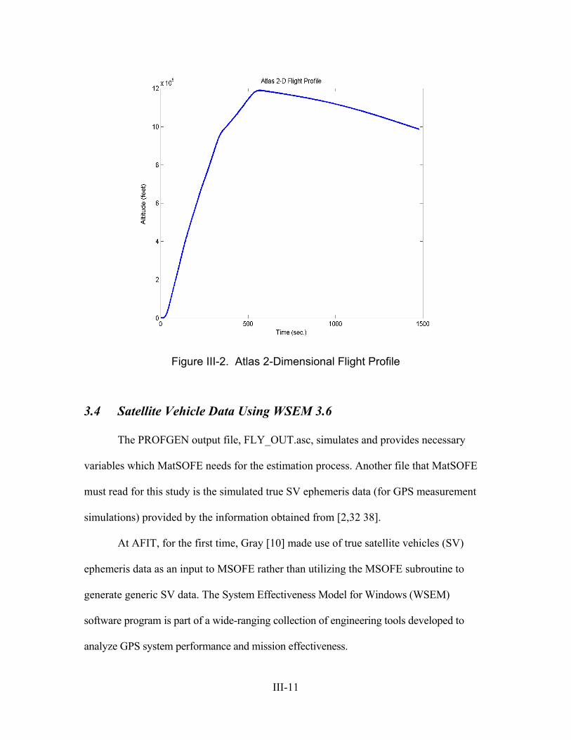
Figure III-2. Atlas 2-Dimensional Flight Profile
3.4 Satellite Vehicle Data Using WSEM 3.6
The PROFGEN output file, FLY_OUT.asc, simulates and provides necessary
variables which MatSOFE needs for the estimation process. Another file that MatSOFE
must read for this study is the simulated true SV ephemeris data (for GPS measurement
simulations) provided by the information obtained from [2,32 38].
At AFIT, for the first time, Gray [10] made use of true satellite vehicles (SV)
ephemeris data as an input to MSOFE rather than utilizing the MSOFE subroutine to
generate generic SV data. The System Effectiveness Model for Windows (WSEM)
software program is part of a wide-ranging collection of engineering tools developed to
analyze GPS system performance and mission effectiveness.
III-11
The WSEM [2] program incorporates a simple computer model of the GPS
system. This software system model includes a simulated Earth based on the World
Geodetic System 1984 (WGS-84) definitions. It also includes up to 32 simulated Navstar
SVs that orbit around the Earth and various types of GPS user equipment (UE )
simulations which the WSEM operator may select and define to be located at any point or
set of points on or near the simulated Earth surface. As part of its GPS system model,
WSEM automatically computes the current Earth-centered, Earth-fixed (ECEF) positions of
each Navstar SV in the constellation defined by the selected almanac data file. "Almanac,"
as used here, refers to a set of orbital parameters that define where a satellite is and where it
is headed. The WSEM's SV almanacs and related mathematical algorithms are
implemented exactly as in the actual GPS system, except that provisions for geostationary
satellite almanacs have also been included. Thus, WSEM is compatible with the
information that the real GPS SVs broadcast on-orbit [2].
The “SEM almanac” used in this study is obtained from the National Geodetic
Survey(NGS)’s continuously operating reference stations (CORS) web site [32]. The SV
ephemeris used in the SNSM simulation was selected based upon the best four SV
available for a random day (the current day when SEM almanac was downloaded) by the
WSEM 3.6 Software [2]. The four SVs chosen were based on:
• Random day (28 July 2001) selected.
(GPS week 1124, Day of year 209).
• GPS Almanac data file "072801A.AL3" (See Appendix E) was obtained
(downloaded) from United States Coast Guard web sites [32, 38].
III-12
• LAT/LONG/ALT along the Tanker flight profile was noted and entered
in WSEM V3.6.
• Best 4 SV based on PDOP algorithm
• 10° mask angle (SV visibility rejection criteria)
• Scenario duration: 1 hour [Begin time 04:00 UTC
(Coordinated Universal Time or 08:00 Eastern time)]
The best four SVs are then numerically displayed to the user. The mask angle was
chosen as 10° based on the author’s experience. Thus, all satellites in view above a 10°
angle made from the GPS antenna surface (mask angle) on 28 July 2001 between the
hours of 04:00 - 06:00 Greenwich mean time are available for use. For further
information on SEM 3.6 software and the SEM 3.6 output plot format, see [2].
3.5 The SNSM Computer Model
The Landing System Model (LSM) and Differential Landing System Model
(DLSM) model [10,6] were used as a reference to model the Space Navigation System
Model (SNSM) computer model. The SNSM is divided into two parts for computer
modeling, the truth model and the filter design model. The truth model represents the
computer-generated simulation of the real-world error characteristics found in avionics
“black boxes” and the environment in which the units operate. The research was
accomplished through computer simulation; therefore, the truth model will simulate the
errors in true avionics hardware (INS, GPS/DGPS, Baro, Radar Altimeter) black boxes.
The truth model generates the measurement updates for the SNSM filter, the true flight
profile of the aircraft, and a state variable baseline for evaluating filter performance
III-13
[10,6]. Detailed explanations related to truth model, filter model, measurement model,
GPS and DGPS error models, etc. will be presented in Sections 3.6.1 and 3.6.2. The truth
model consists of 69 error states for GPS-aided INS and 61error states for DGPS-aided
INS about their nominal values. The filter model represents the SNSM as it could be
hosted on-board an aircraft computer. Briefly, the SNSM filter model is a 13-state
extended Kalman filter developed through order reduction of the original 93-state truth
model of [27,33] for just INS, plus 30 more states for GPS (22 for DGPS). Section 3.6.1
and 3.6.2 of this section explains INS and GPS error models in detail, respectively. An
advantage of using only 13 states is that the current state-of-the-art aircraft host
computers can handle the computational requirements.
The block diagram, Figure III-3, explains the interaction of the filter and truth
model in MatSOFE. A simulated flight profile is provided by PROFGEN [29], and the
U.S. National Geodetic Survey (NGS)’s continuously operating reference stations
(CORS) web page [32] provides true SV ephemeris data for any SV. Use of the "real-
world" ephemeris replaced almost six of the prior m-files functions used in old versions
of MatSOFE. The best four SV, which have the best (lowest) position dilution of
precision (PDOP), were chosen by using System Effectiveness Model for Windows
(WSEM) software [2]. The WSEM36 program requires GPS almanac files to run. Current
Almanac files can be found at the ARINC web site [2] or at the United States Coast
Guard web sites [32, 38]. With this information, the truth model is able to simulate a real
world INS navigation solution, , and generate the real world GPS/DGPS
measurements, RGPS and RDGPS respectively. The Kalman filter block in Figure III-3
represents the SNSM filter. Corrections from the SNSM filter are subtracted from the
INS+x δx
III-14
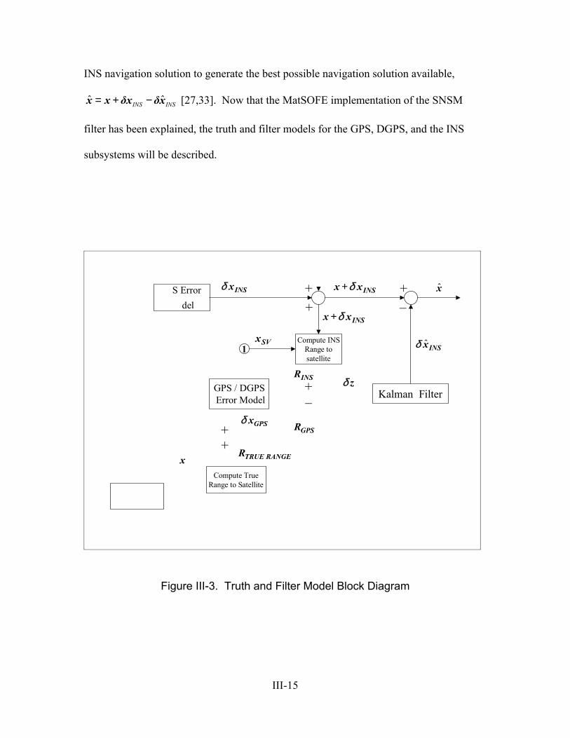
INS navigation solution to generate the best possible navigation solution available,
[27,33]. Now that the MatSOFE implementation of the SNSM
filter has been explained, the truth and filter models for the GPS, DGPS, and the INS
subsystems will be described.
ˆ INS INS= + −x x δx δx
INMo
True SatelliteOrbit Trajectory
True AircraftFlight Trajectory
1 SVx
ˆ
Kalman Filter
S Errordel
GPS / DGPSError Model
Compute INSRange to satellite
INSxδ INSxx δ+
INSxx δ+
INSxδ
GPSxδGPSR
RANGETRUER
zδ
x
1
Compute TrueRange to Satellite
SVx
INSR
x
++
+
++
+
_
_
Figure III-3. Truth and Filter Model Block Diagram
III-15
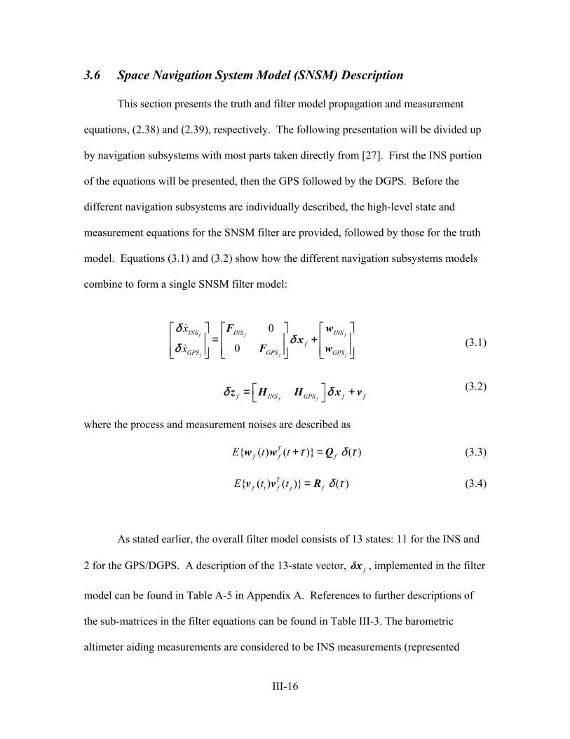
3.6 Space Navigation System Model (SNSM) Description
This section presents the truth and filter model propagation and measurement
equations, (2.38) and (2.39), respectively. The following presentation will be divided up
by navigation subsystems with most parts taken directly from [27]. First the INS portion
of the equations will be presented, then the GPS followed by the DGPS. Before the
different navigation subsystems are individually described, the high-level state and
measurement equations for the SNSM filter are provided, followed by those for the truth
model. Equations (3.1) and (3.2) show how the different navigation subsystems models
combine to form a single SNSM filter model:
0
0f f
f f
INS INS INS
fGPS GPS GPS
x
x
F wx
F w
δδ
δ
=
f
f
+
(3.1)
f ff INS GPS f fδ = δ +z H H x v
)τ
(3.2)
where the process and measurement noises are described as
( ) ( ) (Tf f fE t t τ δ+ =w w Q (3.3)
(3.4) ( ) ( ) ( )Tf i f j fE t t δ τ=v v R
As stated earlier, the overall filter model consists of 13 states: 11 for the INS and
2 for the GPS/DGPS. A description of the 13-state vector, fδx , implemented in the filter
model can be found in Table A-5 in Appendix A. References to further descriptions of
the sub-matrices in the filter equations can be found in Table III-3. The barometric
altimeter aiding measurements are considered to be INS measurements (represented
III-16
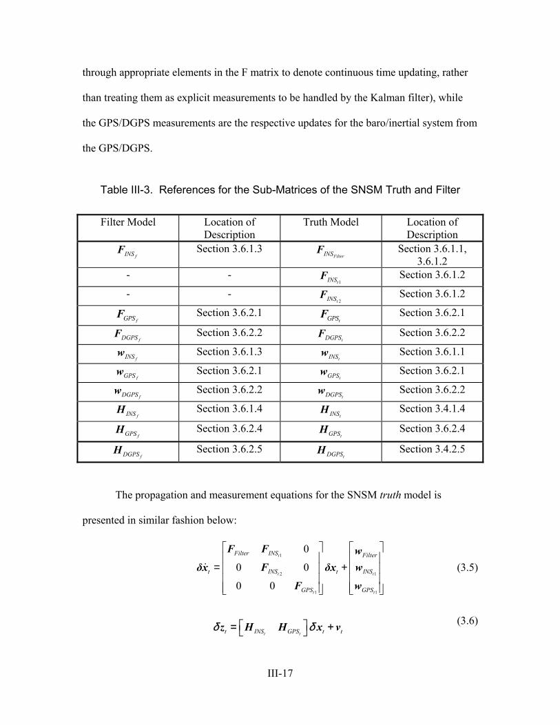
through appropriate elements in the F matrix to denote continuous time updating, rather
than treating them as explicit measurements to be handled by the Kalman filter), while
the GPS/DGPS measurements are the respective updates for the baro/inertial system from
the GPS/DGPS.
Table III-3. References for the Sub-Matrices of the SNSM Truth and Filter
Filter Model Location of Description
Truth Model Location of Description
fINSF Section 3.6.1.3 FilterINSF Section 3.6.1.1,
3.6.1.2 - -
1tINSF Section 3.6.1.2
- - 2tINSF Section 3.6.1.2
fGPSF Section 3.6.2.1 tGPSF Section 3.6.2.1
fDGPSF Section 3.6.2.2 tDGPSF Section 3.6.2.2
fINSw Section 3.6.1.3 tINSw Section 3.6.1.1
fGPSw Section 3.6.2.1 tGPSw Section 3.6.2.1
fDGPSw Section 3.6.2.2 tDGPSw Section 3.6.2.2
fINSH Section 3.6.1.4 tINSH Section 3.4.1.4
fGPSH Section 3.6.2.4 tGPSH Section 3.6.2.4
fDGPSH Section 3.6.2.5 tDGPSH Section 3.4.2.5
The propagation and measurement equations for the SNSM truth model is
presented in similar fashion below:
1
2
1 1
0
0 0
0 0
t
t
t t
Filter INS Filter
t INS t INS
GPS GPS
1t
=
+
F F wδx F δx w
F w
tδ +
(3.5)
t tt INS GPS tδ = z H H x v (3.6)
III-17
The SNSM truth model consists of the original thirteen states of the filter model
(represented by FFilter and wFilter), augmented by additional INS and GPS/DGPS states.
The total number navigation subsystems state is 69: 39 INS states, and 30 GPS states for
GPS integrated systems, and 61: 39 INS states, and 22 DGPS states for DGPS integrated
systems. Table A-1through Table A-4, in Appendix A, provide a full description of each
individual state of the truth model. Table B-1 through Table B-6, and Table B-7 through
Table B-9 in Appendix B have a complete listing of the components of the F elements
and the Q noise strengths associated with the w vector components in Equation (3.5).
There is one crucial difference between the first thirteen states of the filter model
and the first thirteen states of the truth model [27,33]. The filter model dynamics driving
noise and measurement noise do not correlate exactly with those of the first thirteen states
of the truth model. To achieve good tuning against the truth model, the filter model noise
statistics values (Qf and Rf ) have been altered [27,33]. The following sections will
provide a detailed presentation into the exact make-up of the truth and filter model
propagation and measurement equations for all navigation subsystems used in this thesis.
3.6.1 The Inertial Navigation System (INS) Model
This section presents the truth and filter models used for the INS. The INS model
is a strapped-down wander azimuth system that senses aircraft motion via gyros and
accelerometers and is used as the primary source for navigation [27]. The INS model has
been derived from a medium accuracy ring laser gyro (RLG) INS 93-state model [18,33].
First, the original 93-state model will be presented, followed by the reduced-ordered
III-18
39-state truth and 11-state filter models. After the INS truth and filter state equations
have been defined, barometric altimeter measurement equations will be presented.
3.6.1.1 The 93-State LN-93 Error Model
The 93-state Litton INS computer model has been generated by the Wright
Laboratories, Avionics Directorate, Avionics System Integration and Research Team
(ASIRT). Their development uses both past AFIT research and INS vendor [18]
documentation to “fine-tune” past modeling efforts [33,36,43]. The 93-state model
generates a high number of documented error sources that are found in the Litton wander-
azimuth LN-93 INS [18]. These errors are described using six categories of states
[27,33]:
δ δ δ δ δ δ δ = x x x x x x xTT T T T T T
1 2 3 4 5 6 (3.7)
where is a 93 × 1 column vector and: δ x
1δ x : represents the "general" error vector containing 13 position, velocity,
attitude, and vertical channel errors (representative of a Pinson 9-state
model of INS error characteristics augmented with 4 altimeter error
states).
2δ x : consists of 16 gyro, accelerometer, and baro-altimeter exponentially time-
correlated errors, and "trend" states. These states are modeled as first
order Markov processes in the truth (system) model.
III-19
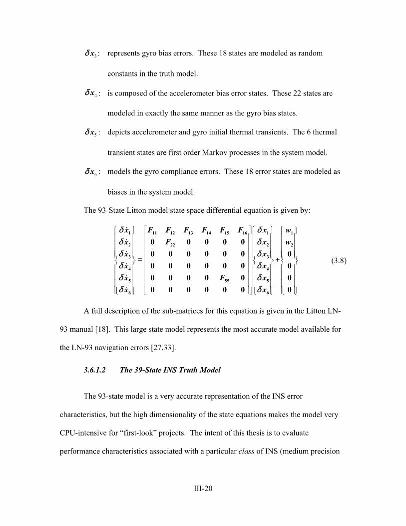
3δ x : represents gyro bias errors. These 18 states are modeled as random
constants in the truth model.
4δ x : is composed of the accelerometer bias error states. These 22 states are
modeled in exactly the same manner as the gyro bias states.
5δ x : depicts accelerometer and gyro initial thermal transients. The 6 thermal
transient states are first order Markov processes in the system model.
6δ x : models the gyro compliance errors. These 18 error states are modeled as
biases in the system model.
The 93-State Litton model state space differential equation is given by:
δ δδ δδ δδ δδ δδ δ
= +
x F F F F F F x wx F x wx xx xx Fx x
1 11 12 13 14 15 16 1 1
2 22 2 2
3 3
4 4
5 55
6 6
0 0 0 0 00 0 0 0 0 0 00 0 0 0 0 0 00 0 0 0 0 00 0 0 0 0 0 0
x5
(3.8)
A full description of the sub-matrices for this equation is given in the Litton LN-
93 manual [18]. This large state model represents the most accurate model available for
the LN-93 navigation errors [27,33].
3.6.1.2 The 39-State INS Truth Model
The 93-state model is a very accurate representation of the INS error
characteristics, but the high dimensionality of the state equations makes the model very
CPU-intensive for “first-look” projects. The intent of this thesis is to evaluate
performance characteristics associated with a particular class of INS (medium precision
III-20
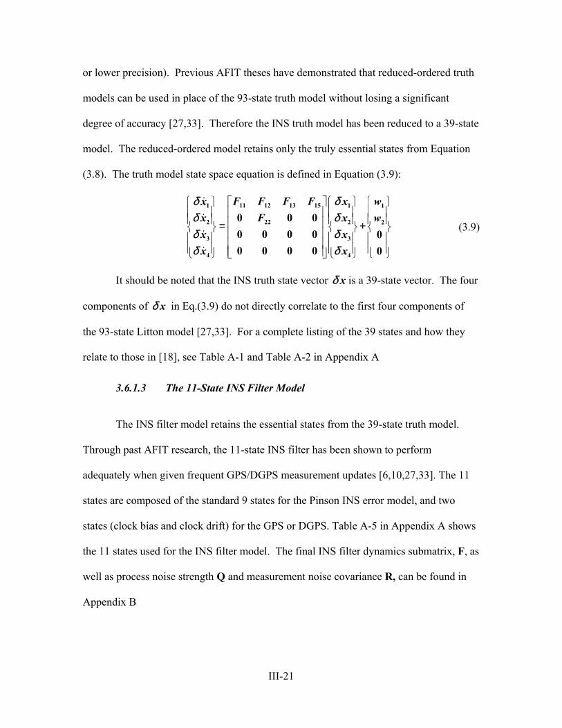
or lower precision). Previous AFIT theses have demonstrated that reduced-ordered truth
models can be used in place of the 93-state truth model without losing a significant
degree of accuracy [27,33]. Therefore the INS truth model has been reduced to a 39-state
model. The reduced-ordered model retains only the truly essential states from Equation
(3.8). The truth model state space equation is defined in Equation (3.9):
δ δδ δδδ δ
δ
= +
F F F Fx x wFx x w
xx x
11 12 13 151 1 1
222 2 2
3 3
4 4
0 0 00 0 0 0 00 0 0 0 0
x (3.9)
It should be noted that the INS truth state vector is a 39-state vector. The four
components of in Eq.(3.9) do not directly correlate to the first four components of
the 93-state Litton model [27,33]. For a complete listing of the 39 states and how they
relate to those in [18], see Table A-1 and Table A-2 in Appendix A
δ x
δ x
3.6.1.3 The 11-State INS Filter Model
The INS filter model retains the essential states from the 39-state truth model.
Through past AFIT research, the 11-state INS filter has been shown to perform
adequately when given frequent GPS/DGPS measurement updates [6,10,27,33]. The 11
states are composed of the standard 9 states for the Pinson INS error model, and two
states (clock bias and clock drift) for the GPS or DGPS. Table A-5 in Appendix A shows
the 11 states used for the INS filter model. The final INS filter dynamics submatrix, F, as
well as process noise strength Q and measurement noise covariance R, can be found in
Appendix B
III-21
3.6.2 The Global Positioning System (GPS) Model
The GPS navigation system used is based on electromagnetic signals transmitted
from orbiting GPS satellites. This model has been developed throughout research at
AFIT, and many of its fundamental concepts are addressed in a variety of sources
[6,10,27,33,36]. GPS generates navigation information by acquiring the range to
multiple satellites of known position, called “pseudoranges”. Inherent in the
pseudorange are errors caused by ionospheric and tropospheric delays, satellite clock
biases, receiver noise, and ephemeris errors [25,34]. These errors work together to dilute
the accuracy of standard GPS to a level of a couple of meters, depending on the range
resolution technique being used. By incorporating the differential corrections to the
standard GPS pseudoranges, one can achieve much higher navigation precision. Several
error sources can be eliminated or significantly reduced because these errors are common
to both the reference station receiver and the user’s receiver. These errors are composed
of the satellite’s clock error, errors in the satellites’s broadcasted ephemeris data, and
signal propagation delays that are not accounted for by the receiver’s measurements or
modeling. When two receivers in the same vicinity (within about 100 nautical miles) are
using the same set of four satellites, the above errors will be common to both and can be
removed or essentially eliminated by differential techniques [25,34]. The navigation
information passed to the SNSM filter is the respective range and ephemeris data position
to each of four satellites, with differential corrections applied to provide more accurate
information [33]. The next four sections present all the necessary equations to define the
GPS and DGPS truth, and associated filter error models fully.
III-22
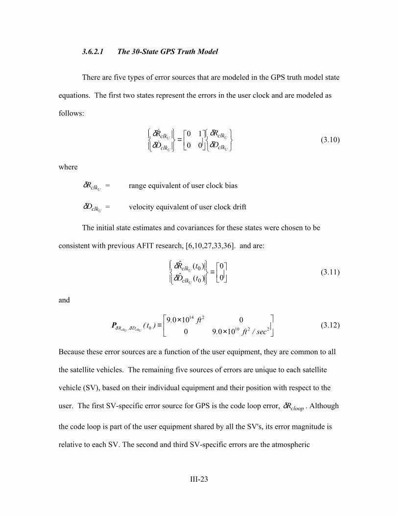
3.6.2.1 The 30-State GPS Truth Model
There are five types of error sources that are modeled in the GPS truth model state
equations. The first two states represent the errors in the user clock and are modeled as
follows:
δδ
δδ
RD
RD
clk
clk
clk
clk
U
U
U
U
=
0 10 0
(3.10)
where
δRclkU = range equivalent of user clock bias
δDclkU = velocity equivalent of user clock drift
The initial state estimates and covariances for these states were chosen to be
consistent with previous AFIT research, [6,10,27,33,36]. and are:
(3.11) δδ
( )( )
R tD t
clk
clk
U
U
0
0
00
=
and
(3.12) 14 2
0 10 2 2
9 0 10 00 9 0 10clk clkU UR , D
. ft( t )
. ft / sec ×
= × Pδ δ
Because these error sources are a function of the user equipment, they are common to all
the satellite vehicles. The remaining five sources of errors are unique to each satellite
vehicle (SV), based on their individual equipment and their position with respect to the
user. The first SV-specific error source for GPS is the code loop error, δRcloop . Although
the code loop is part of the user equipment shared by all the SV's, its error magnitude is
relative to each SV. The second and third SV-specific errors are the atmospheric
III-23
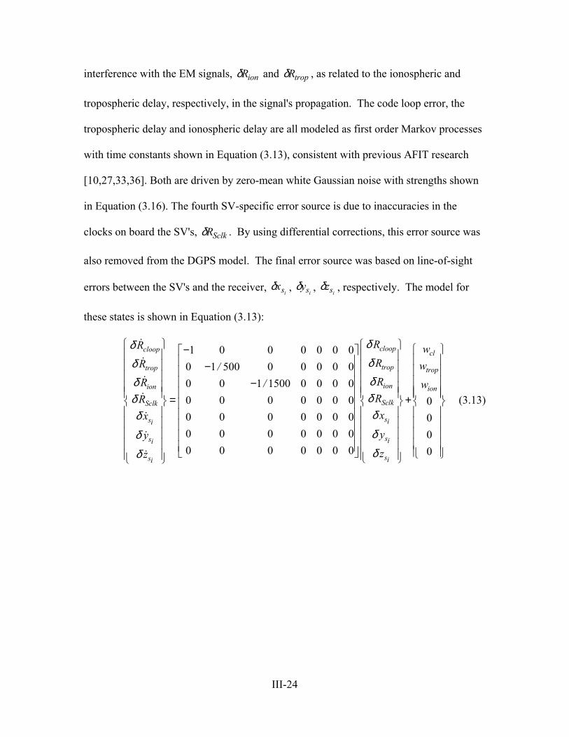
interference with the EM signals, δRion and δRtrop , as related to the ionospheric and
tropospheric delay, respectively, in the signal's propagation. The code loop error, the
tropospheric delay and ionospheric delay are all modeled as first order Markov processes
with time constants shown in Equation (3.13), consistent with previous AFIT research
[10,27,33,36]. Both are driven by zero-mean white Gaussian noise with strengths shown
in Equation (3.16). The fourth SV-specific error source is due to inaccuracies in the
clocks on board the SV's, δRSclk . By using differential corrections, this error source was
also removed from the DGPS model. The final error source was based on line-of-sight
errors between the SV's and the receiver, δxsi, δysi
, δzsi
00 0
0 0 0 0 00 00 00 00 0
, respectively. The model for
these states is shown in Equation (3.13):
1 01
00 00 00 00 0
/−0
050
0000
01−
(3.13)
0 0 00 500 00 1
0 00 00 00 0
cloopcloop
troptrop
ionion
SclkSclk
ss ii
ss ii
ss ii
RRRRRR /RRxx
yy
zz
δδδδδδδδδδδδδδ
− =
0000
cl
trop
ion
ww
w
+
III-24
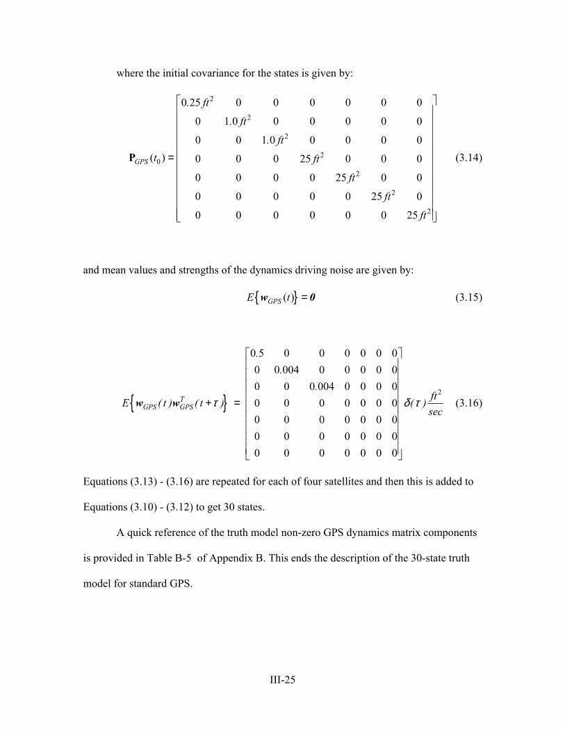
where the initial covariance for the states is given by:
2
2
2
20
2
2
2
0 25 0 0 0 0 0 0
0 1 0 0 0 0 0 0
0 0 1 0 0 0 0 0( ) 0 0 0 25 0 0 0
0 0 0 0 25 0 0
0 0 0 0 0 25 0
0 0 0 0 0 0 25
GPS
. ft
. ft
. ftt ft
ft
ft
ft
=
P (3.14)
and mean values and strengths of the dynamics driving noise are given by:
( )GPSE t =w 0 (3.15)
2
0 5 0 0 0 0 0 00 0 004 0 0 0 0 00 0 0 004 0 0 0 00 0 0 0 0 0 00 0 0 0 0 0 00 0 0 0 0 0 00 0 0 0 0 0 0
TGPS GPS
..
.ftE ( t ) ( t ) ( )sec
+ =
w w τ δ τ (3.16)
Equations (3.13) - (3.16) are repeated for each of four satellites and then this is added to
Equations (3.10) - (3.12) to get 30 states.
A quick reference of the truth model non-zero GPS dynamics matrix components
is provided in Table B-5 of Appendix B. This ends the description of the 30-state truth
model for standard GPS.
III-25
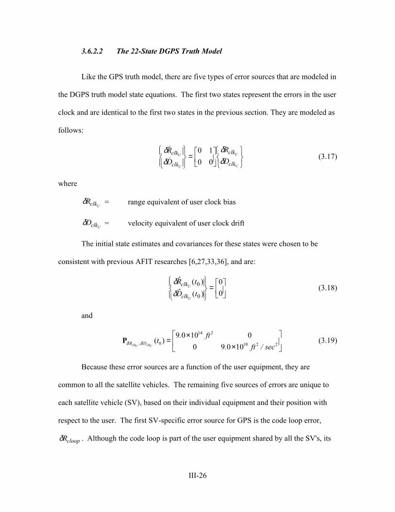
3.6.2.2 The 22-State DGPS Truth Model
Like the GPS truth model, there are five types of error sources that are modeled in
the DGPS truth model state equations. The first two states represent the errors in the user
clock and are identical to the first two states in the previous section. They are modeled as
follows:
(3.17) δδ
δδ
RD
RD
clk
clk
clk
clk
U
U
U
U
=
0 10 0
where
δRclkU = range equivalent of user clock bias
δDclkU = velocity equivalent of user clock drift
The initial state estimates and covariances for these states were chosen to be
consistent with previous AFIT researches [6,27,33,36], and are:
(3.18) δδ
( )( )
R tD t
clk
clk
U
U
0
0
00
=
and
14 2
0 10 2 2
9 0 10 0( )
0 9 0 10clk clkU UR , D. ft
t. ft / sec
×= ×
δ δP (3.19)
Because these error sources are a function of the user equipment, they are
common to all the satellite vehicles. The remaining five sources of errors are unique to
each satellite vehicle (SV), based on their individual equipment and their position with
respect to the user. The first SV-specific error source for GPS is the code loop error,
δRcloop . Although the code loop is part of the user equipment shared by all the SV's, its
III-26
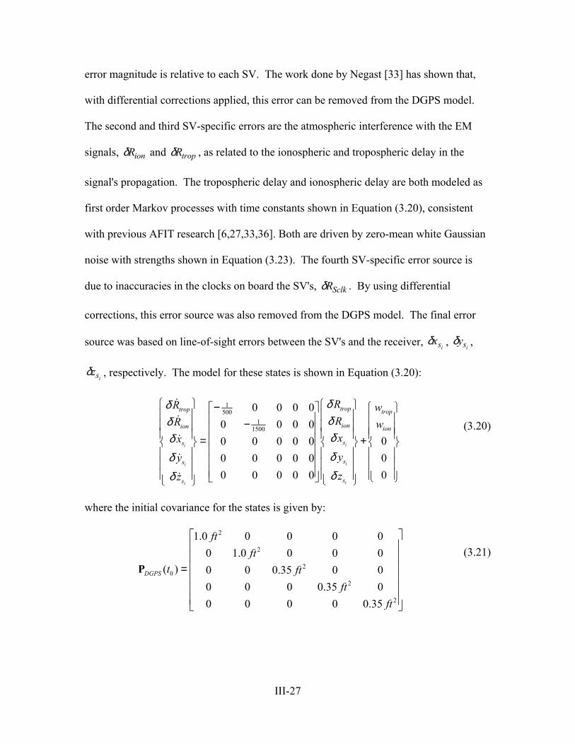
error magnitude is relative to each SV. The work done by Negast [33] has shown that,
with differential corrections applied, this error can be removed from the DGPS model.
The second and third SV-specific errors are the atmospheric interference with the EM
signals, δRion and δRtrop , as related to the ionospheric and tropospheric delay in the
signal's propagation. The tropospheric delay and ionospheric delay are both modeled as
first order Markov processes with time constants shown in Equation (3.20), consistent
with previous AFIT research [6,27,33,36]. Both are driven by zero-mean white Gaussian
noise with strengths shown in Equation (3.23). The fourth SV-specific error source is
due to inaccuracies in the clocks on board the SV's, δRSclk . By using differential
corrections, this error source was also removed from the DGPS model. The final error
source was based on line-of-sight errors between the SV's and the receiver, δxsi, δysi
,
δzsi, respectively. The model for these states is shown in Equation (3.20):
00 0
000
i
i
i
trop
ion
s
s
s
RRx
y
z
δδδδδ
i
i
i
trop
ion
s
s
s
RRx
y
z
δδδδδ
0( )t2
000
0.350
ft=P
1500
11500
0 0 00 0
00 0 0 000 0 0 000 0 0 0
trop
ion
ww
− − = +
(3.20)
where the initial covariance for the states is given by:
2
2
2
2
1.0 0 0 00 1.0 0 00 0 0.35 00 0 0 00 0 0 0.35
DGPS
ftft
ft
ft
(3.21)
III-27
and mean values and strengths of the dynamics driving noise are given by:
( )DGPSE t =w 0 (3.22)
2
0.001 0 0 0 00 0.0004 0 0 0
( ) ( ) ( )0 0 0 0 0sec
0 0 0 0 00 0 0 0 0
TDGPS DGPS
ftE t t
+ =
w w τ δ
τ
clk
lk
(3.23)
The reduced dynamic driving noise strengths from standard GPS are indicative of
the error reduction for these remaining states when differential corrections are applied. A
quick reference of the truth model non-zero DGPS dynamics matrix components is
provided in Table B-6 of Appendix B This ends the description of the 22-state truth
model for DGPS. Now the filter model will be presented.
3.6.2.3 The 2-State GPS/DGPS Filter Model
Various research efforts have shown that two states provide a sufficient model for
GPS and DGPS [6 10,27,33,36,43]. The primary argument is that the errors modeled by
the other states in the previous two sections are small when compared to the two states
common to all SV's. By adding dynamics driving noise, of strength Q, and re-tuning the
filter, the overall performance of the DLSM can be maintained with the significantly
reduced-order model of Equation (3.24):
(3.24) 0 10 0
UU
U cU
clk Rclk
clk Dclk
R wRD wD
= +
δδδδ
III-28
The values implemented for the dynamics driving noise strengths can be found in
Tables B-10 through B-12 of Appendix B. It should be noted that, in the tuning process,
the measurement noise covariance values R (as shown in Appendix B) have also been
adjusted to achieve adequate tuning of the filter [20]. This completes the description of
the GPS/DGPS filter model. The next section presents the GPS/DGPS measurement
equations for both the truth and the filter models.
3.6.2.4 GPS Measurement Model
There are four GPS measurement updates, one for each of the satellite
pseudorange signals received by the SNSM filter. These measurement updates are once
again difference measurements. First the DGPS truth model difference measurement will
be fully presented, followed by a brief description of the filter measurement model.
The GPS difference measurement is formed by taking the difference of the INS-
calculated pseudorange, and actual pseudorange, RINS GPSR :
(3.25) GPS INS GPSz R Rδ = −
The real pseudorange, GPSR is the sum of the true range from the user to the satellite plus
all the errors in the pseudorange signal propagation. The measurement equation is
modeled as:
GPS t cloop trop ion Sclk UclkR R R R R R R= + + + + + −δ δ δ δ δ v (3.26)
where
GPSR = GPS pseudorange measurement, from SV to user
Rt = true range, from SV to user
III-29
cloopRδ = range error due to code loop error
tropRδ = range error due to tropospheric delay
δRion = range error due to ionospheric delay
SclkRδ = range error due to SV clock error
δRUclk = range error due to user clock error
v = zero-mean white Gaussian measurement noise
Note that, since v is assumed zero-mean, white Gaussian noise, statistically
speaking, one can choose v with either a plus "+" or minus "-" coefficent in Equation
(3.26). The author chooses the coefficient carefully so that the end result shows a plus "+
v" sign in Equation (3.31) and Equation (3.32).
The second source of a range measurement is the INS itself, RINS [27,33]. RINS is
the difference between the SNSM-calculated position, XU and the satellite position from
the ephemeris data XS. This difference vector is represented below in the ECEF frame
e eU S
INS U S U S
U S
x xR y
z zy
= − = −
X X (3.27)
An equivalent form for Equation (3.27)) is
2 2( ) ( ) (INS U S U S U S2)R x x y y z z= − + − + − (3.28)
Based on Assumption xiv from Chapter 1, Equation (3.28) can be approximated
and rewritten in terms of the true range and a truncated first-order Taylor series, with
perturbations representing the errors in XU and XS:
III-30
, ,
( , ) ( , )( ) ( )
INS S U INS S UINS t U S
U SS U S U nomnom
R RR R= + ⋅ + ⋅X X X XX XX XX X X X
∂ ∂δ δ∂ ∂ (3.29)
The solution for RINS is found by substituting Equations (3.28) into Equation (3.29) and
evaluating the partial derivatives to get [27,33].
R R x xR
x y yR
y z zR
z
x xR
x y yR
y z zR
z
INS tS U
INSU
S U
INSU
S U
INSU
S U
INSS
S U
INSS
S U
INSS
= − −
⋅ − −
⋅ − −
⋅
+ −
⋅ + −
⋅ + −
⋅
δ δ
δ δ δ
δ
(3.30)
Finally, the GPS pseudorange truth model difference measurement is given as:
GPS INS GPStz R Rδ = −
S U S U S UU U
INS INS INS
S U S U S US S
INS INS INS
x x y y z zU
S
x yR R R
x x y y z z
z
x y zR R R
− − −= − ⋅ − ⋅ − ⋅
− − −+ ⋅ + ⋅ + ⋅
δ δ
δ δ
δ
δ
(3.31)
[1] [1] [1] [1] [1]trop ion Uclk cloop SclkR R R R R− − − − −δ δ δ δ δ v+
The user position errors in Equation (3.31) can be derived from the first three states of the
filter or truth model using an orthogonal transformation [27,33].
The filter design model for the GPS measurement will now be derived. Since
the filter model does not contain the states for the errors in the satellite position, these
terms are removed from the equation. The filter model measurement equation can
therefore be written as:
III-31
GPS INS GPSfz R Rδ = −
= − −
⋅ − −
⋅ − −
⋅
− +
x xR
x y yR
y z zR
z
R v
S U
INSU
S U
INSU
S U
INSU
Uclk
δ δ
δ[ ]1
δ (3.32)
The filter measurement noise variance, R, will be tuned to attain adequate
performance despite the reduction in order from the truth model and despite the
approximation of the truncated Taylor series. The measurement noise variances for both
the filter and the truth model equations are provided in Table B-13 of Appendix B. This
completes the description of the GPS measurement equations and the entire SNSM filter
and truth model equations for a standard GPS-aided INS.
3.6.2.5 DGPS Measurement Model
There are four differentially corrected GPS measurement updates, one for each of
the satellite range signals received by the SNSM filter. These measurement updates are
once again difference measurements. First the DGPS truth model difference
measurement will be fully presented, followed by a brief description of the filter
measurement. The DGPS difference measurement is formed by taking the difference of
the INS-calculated pseudorange, and actual pseudorange, RINS DGPSR .
DGPS INS DGPSz R Rδ = − (3.33)
The real pseudorange, DGPSR is the sum of the true range from the user to the
satellite plus all the errors in the pseudorange signal propagation. After differential
corrections are applied, the measurement equation is modeled as:
DGPS t trop ion UclkR R R R R= + + + −δ δ δ v (3.34)
III-32
where
DGPSR = Differentially corrected GPS pseudorange measurement, from SV to
user
Rt = true range, from SV to user
tropRδ = range error due to tropospheric delay
δRion = range error due to ionospheric delay
δRUclk = range error due to user clock error
v = zero-mean white Gaussian measurement noise
A development analogous to equations (3.27) through (3.30) can be accomplished, and
finally, the DGPS pseudorange truth model difference measurement is given as:
tDGPS INS DGPSz R Rδ = −
[1] [1] [1]
S U S U S UU U
INS INS INS
S U S U S US S
INS INS INS
trop ion Uclk
x x y y z zU
S
x y zR R R
x x y y z zx y zR R R
R R R v
δ δ
δ δ
δ δ δ
− − −= − ⋅ − ⋅ − ⋅
− − −+ ⋅ + ⋅ + ⋅
− − − +
δ
δ (3.35)
As before, the user position errors in Equation (3.35) can be derived from the first
three states of the filter or truth model using an orthogonal transformation [27,33].
The filter design model for the DGPS measurement will now be derived. Since
the filter model does not contain the states for the errors in the satellite position, these
terms are removed from the equation. The filter model measurement equation can
therefore be written as:
III-33
fDGPS INS DGPSz R Rδ = −
= − −
⋅ − −
⋅ − −
⋅
− +
x xR
x y yR
y z zR
z
R v
S U
INSU
S U
INSU
S U
INSU
Uclk
δ δ
δ[ ]1
δ (3.36)
The filter measurement noise variance, R, will be tuned to attain adequate
performance despite the reduction in order from the truth model and despite the
approximation of the truncated Taylor series. The measurement noise variances for both
the filter and the truth model equations are provided in Table B-13 of Appendix B. This
completes the description of the DGPS measurement equations and the entire SNSM
filter and truth model equations.
3.7 Chapter Summary
This chapter presents the set-up of the SNSM MatSOFE computer simulation.
An introduction to MatSOFE, the WSEM software, and PROFGEN is provided. The
truth model and filter model propagation and measurement equations are described for
the INS/Baro, GPS, and DGPS subsystems. The INS/Baro, GPS, and DGPS truth model
is located in tabular form in Appendix A. The dynamic submatrices FFilter, FINSt1, FINSt2,
FGPS , FDGPS , and process noise strength and measurement noise covariance matrices for
filter and truth models are presented in Appendix B Results and analysis of the SNSM
simulation are presented in Chapter 4.
III-34
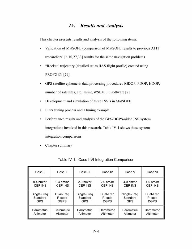
IV. Results and Analysis
This chapter presents results and analysis of the following items:
•
•
•
•
•
•
•
Validation of MatSOFE (comparison of MatSOFE results to previous AFIT
researchers’ [6,10,27,33] results for the same navigation problem).
“Rocket” trajectory (detailed Atlas IIAS flight profile) created using
PROFGEN [29].
GPS satellite ephemeris data processing procedures (GDOP, PDOP, HDOP,
number of satellites, etc.) using WSEM 3.6 software [2].
Development and simulation of three INS’s in MatSOFE.
Filter tuning process and a tuning example.
Performance results and analysis of the GPS/DGPS-aided INS system
integrations involved in this research. Table IV-1 shows these system
integration comparisons.
Chapter summary
Table IV-1. Case I-VI Integration Comparison
Case I Case II Case III Case IV Case V Case VI
0.4 nm/hr CEP INS
0.4 nm/hr CEP INS
2.0 nm/hr CEP INS
2.0 nm/hr CEP INS
4.0 nm/hr CEP INS
4.0 nm/hr CEP INS
Single-Freq Standard
GPS
Dual-Freq P-code DGPS
Single-Freq Standard
GPS
Dual-Freq P-code DGPS
Single-Freq Standard
GPS
Dual-Freq P-code DGPS
Barometric Altimeter
Barometric Altimeter
Barometric Altimeter
Barometric Altimeter
Barometric Altimeter
Barometric Altimeter
IV-1
4.1 Validation of MATSOFE
This research is a follow-on effort of Gray [10] and Britton [11]. There are some
similarities along with variations between their studies and this study. They both studied
a GPS/DGPS-aided LN-93 INS [18] integrated systems for precision landing approaches.
It has seen that the truth models and filter design error models they used for INS and GPS
have been utilized in AFIT for more than 8 years as validated models, and consequently
they are used as validated and reliable references in terms of truth and filter model for
both INS and GPS/DGPS including truth/filter measurements models in this research. On
the contrary, this research dealt with evaluating position accuracy for a launch vehicle
rather than accurate GPS/INS integrations for a precision landing or airborne navigation
application.
To accomplish the performance analysis of a GPS-aided INS system, one has to
make Monte Carlo simulations and/or covariance analyses. As an international officer,
the author was not eligible to make use of the MSOFE software [30]. MSOFE is
restricted to use by U.S. government agencies and their U.S. contractors. At the
beginning it was not a considerable concern, but as time passed, generating and
validating a performance evaluation tool became the biggest issue of this study. That is
because, up to now, AFIT students have been accustomed to utilize MSOFE [30] as a
performance evaluation tool. For that reason, first of all, the modified MatSOFE needs to
be validated as a reliable performance evaluation tool. The most effective way of
validating MatSOFE was to take previous researchers’ data as an input to MatSOFE. If it
gives comparable outputs to the same inputs, then it would be validated.
IV-2
To start, the original MatSOFE was revised to handle more complicated
navigation system problems, like INS/GPS/BARO integrated navigation system with
higher-state and realistic truth model definitions, rather than an INS only navigation
system designed for a simple specific problem with short flight durations. It especially
was not convenient for this study in terms of truth and filter model state dimensions,
“Pinson error model” definition, and the GPS data used. For more information about
MatSOFE and revisions made to MatSOFE, see Chapter 3.2, Introduction to MatSOFE.
The next step was generating necessary simulated INS and GPS ephemeris data
(Sections 4.2 and 4.3 discuss the INS and GPS data simulation process in detail). For that
reason, the exact tanker aircraft profile, FLY_OUT file (FLY_OUT is the output file of
the PFOFGEN) is regenerated by using the provided PROF_IN file (PROF_IN is the
input file for profile generator, PROFGEN [29]) in Gray’s thesis [10]. This regenerated
tanker aircraft flight profile has been used throughout the MatSOFE validation process.
The first MatSOFE simulation run is accomplished by using all Gray’s [10] inputs, same
FLY_OUT file for tanker aircraft and the same day of simulated “true” GPS ephemeris
data. A similar approach is tracked for Britton [6] inputs, concerning the cases with
DGPS integration, by using the same simulation model except for implementing DGPS
into system rather than standard GPS. Then the validation scope is extended utilizing
Mosle’s [27] and Negast’s [33] inputs as well. The next and succeeding sections will
discuss comparison between original outputs they have presented in their theses by
utilizing MSOFE as an evaluation tool, and MatSOFE generated outputs for the same set
of circumstances. By saying “the same set of circumstances”, the author means utilizing
the same F, Q, H, and R values as used by those previous researchers for both filter and
IV-3
the truth model. As mentioned earlier, the same error models for LN-93 inertial
navigation system, PROFGEN output (FLY_OUT file), and simulated GPS data are also
generated for comparison cases.
4.1.1 Comparison to Gray’s Results [10]
A GPS-integrated navigation system, using a 0.4 nm/hr CEP INS with baro-
altimeter incorporated, was a common study case to almost all previous AFIT researchers
being tracked [6,10,27,33]. Gray’s first research case and this research’s first case are
exactly the “same” study cases, except for the flight profile (PROFGEN data) used.
Actually, creating a simulation case close enough to his case depends on the information
he declared in his thesis. During the comparison phase, some additional information was
needed to duplicate their work to reflect the same characteristics, like USOFE code
(USOFE is the user-controlled portion of MSOFE), filter and truth model initial state and
covariance values, etc. It is almost impossible to reproduce the identical or exactly same
simulation conditions for validation purposes, but the author has confidence that the
reproduced models represent their work effectively.
Figure G-1 and Figure G-2 in Appendix G show the MatSOFE-generated and
MSOFE-generated outputs for the same simulation case, respectively. Only position error
plots are shown in Appendix G. For more detailed comparison, see Gray’s thesis [10].
Under the same simulation conditions, MatSOFE consistently generates positions errors
that are almost twice as accurate as the MSOFE results. The encouraging thing about this
result is that it is not close enough to say “same” in terms of position accuracy, but at
least it is not worse. This phenomenon has also seen in comparison to Mosle’s [27]
IV-4
work. The first approach to solve that problem was to regenerate the simulated GPS
ephemeris data because this result has not been seen in comparison to Britton’s results
(Britton did the same study as Gray except for using DGPS instead of GPS).
Regenerating GPS data didn’t solve the problem. There are two reasonable explanations
for what might cause that difference between MatSOFE results, and that of Gray’s and
Mosle’s cases. Mosle implemented the USOFE subroutines “ ORBIT” and “CALCDOP”
for GPS data simulation rather than simulate true GPS ephemeris data in his research. It
is believed that might cause that disagreement in comparison. In contrast, Gray was the
first researcher in AFIT to put the simulated true GPS ephemeris data into practice, but
there are inconsistencies found between what he stated in his thesis and what was written
in his USOFE code (e.g., some of his thesis filter process noise (Qf) values don’t agree
either with his USOFE code values or with Britton’s values.) That might be the
explanation for the disagreement in comparison with Gray’s study. Insufficient
conversion from MSOFE into MatSOFE could also be accepted as another reasonable
explanation to the disagreement experienced, because, as mentioned before, reproducing
someone else’s study environment is highly dependent on the information gathered,
related to this study. The author has never been able to look at the original MSOFE code,
with the result that he could not ensure the removal of any discrepancies between it and
the MatSOFE implementation. MatSOFE outputs for the same case as Mosle’s [27]
values are presented later in Figure G-5 of Appendix G.
IV-5
4.1.2 Comparison to Britton’s Results [6]
The inconsistency faced in the GPS-related comparison to Gray has not been
experienced with Britton’s DGPS-aiding 0.4 nm/hr CEP INS case with internal baro-
altimeter aiding. As a matter of fact, Britton had the same study case just like others
(Gray, Mosle, and Negast) except for P-code dual frequency DGPS aiding the INS rather
standard GPS. The MatSOFE-generated results for the DGPS-aided INS integrated
navigation system evaluation are close enough to be declared as accurate as the MSOFE-
generated one (see Figure G-3 and Figure G-4). This accuracy agreement with Britton
study was convincing enough to believe that MatSOFE is a reliable performance
evaluation tool for navigation system problems. For now, pronouncing that MatSOFE is
an evaluation tool as powerful as MSOFE would be an extremely optimistic conclusion.
But, Matlab-based MatSOFE can be upgraded to the same or even higher level as
MSOFE in the future, because Matlab is quite a powerful programming language to
handle difficult computations.
One common thing faced in all the comparison cases was that the previous
researchers preferred slightly conservative tuning for their performance evaluations.
Mosle [27] explains the reason for this choice in his thesis as: “ The conservative nature
of this tuning proved to be necessary to maintain good tracking of the most important
navigation states.” This choice of tuning may be necessary for a precise and intensive
navigation problem, like the precision landing system, but fine (non-conservative) tuning
is preferred for the rocket navigation problem studied in this research.
IV-6
4.2 The Launch Vehicle (Atlas IIAS) Flight Profile
It was a requirement to regenerate the “Tanker” aircraft profile for validation of
MatSOFE to duplicate the previous studies in MatSOFE. Therefore, a PROF_IN file
(PROF_IN is the input file for profile generator software, PROFGEN [29]) is created first
based on the inputs that Gray [10] provided in his thesis (the actual PROF_IN file used to
generate Tanker profile can be found in Gray’s thesis in Appendix C of Gray’s thesis.)
Although a lot of insights into PROFGEN were gained in the Tanker aircraft
profile generation, a personal interview was conducted with Dr. Tragesser [39] of the
AFIT Department of Aeronautics and Astronautics and a sample rocket (Delta II)
PROF_IN file was requested from Dr. Stanton Musick [31] of the Air Force Research
Laboratory prior to generating the launch vehicle profile. PROFGEN reads in the
PROF_IN file, and outputs a binary flight profile output variables file (user-selected
variables, see Table III-1) called “FLY_OUT.asc”.
As discussed earlier, the launch vehicle is simulated by assuming it to be launched
from Cape Canaveral AS, SLC-41, with the following initial conditions:
Initial latitude 028.5 N•
•
•
•
Initial longitude 081.0 W
Initial altitude 0 feet
Initial ground path heading 90 00.
All initial conditions, flight segments and durations, and user-selected input and
output variables and their units, etc. are all presented in Appendix C. Also, Table IV-2
shows the actual launch operation sequence of the Atlas IIAS. With the assumption of
executing launch operations from Cape Canaveral AS, two available orbit inclination
IV-7
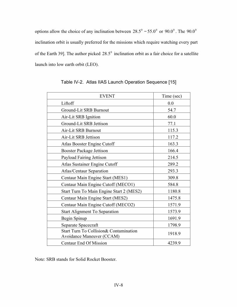
options allow the choice of any inclination between or . The 90
inclination orbit is usually preferred for the missions which require watching every part
of the Earth 39]. The author picked inclination orbit as a fair choice for a satellite
launch into low earth orbit (LEO).
00 0.555.28 − 00.90 00.
05.28
Table IV-2. Atlas IIAS Launch Operation Sequence [15]
EVENT Time (sec) Liftoff 0.0 Ground-Lit SRB Burnout 54.7 Air-Lit SRB Ignition 60.0 Ground-Lit SRB Jettison 77.1 Air-Lit SRB Burnout 115.3 Air-Lit SRB Jettison 117.2 Atlas Booster Engine Cutoff 163.3 Booster Package Jettison 166.4 Payload Fairing Jettison 214.5 Atlas Sustainer Engine Cutoff 289.2 Atlas/Centaur Separation 293.3 Centaur Main Engine Start (MES1) 309.8 Centaur Main Engine Cutoff (MECO1) 584.8 Start Turn To Main Engine Start 2 (MES2) 1180.8 Centaur Main Engine Start (MES2) 1475.8 Centaur Main Engine Cutoff (MECO2) 1571.9 Start Alignment To Separation 1573.9 Begin Spinup 1691.9 Separate Spacecraft 1798.9 Start Turn To Collision& Contamination Avoidance Maneuver (CCAM) 1918.9
Centaur End Of Mission 4239.9
Note: SRB stands for Solid Rocket Booster.
IV-8
4.3 Development of the Three Types of INS’s
The three grades of INS (0.4, 2.0, and 4.0 nm/hr CEP INS) are assumed to be
good representative of military grade, commercial grade, and less expensive (possible
MEMS in a few years) Inertial Navigation Systems. For navigation problems like rocket
launch, it is believed and assumed that INS and GPS sensors will always be redundant.
From this assumption, and taking the chosen orbit (LEO) into account, there comes
another assumption: no GPS outages. Now it can be clearly said that the GPS will be the
dominant system, and overall position accuracy will be dictated by GPS accuracy
performance. Despite the facts mentioned above, the three grades of INS are included in
the research scope. It is believed that the results obtained in each of the cases will be a
useful reference for ongoing research and development efforts.
Gray [10] says that he developed good models for the three grades of INS with
the modifications he made to the initial system covariance matrix by only altering the
random constant shaping filter states (and not changing the 1st order Gauss-Markov drift
states, etc.). Unfortunately, inconsistencies are found between what he stated in his thesis
and what was found in his USOFE code (user-controlled , problem-specific portion of
MSOFE code for simulation). He says that he altered the initial covariance conditions of
the system, but they are all zeroed out in his USOFE code. When what he said in his
thesis is exactly applied in MatSOFE, the filter estimation goes unstable after about100
sec of flight. Then, after personal discussions with Dr. Maybeck (thesis advisor) and Dr.
Musick [31], it was decided that system process noise values (Qs) should be altered rather
than initial covariance to simulate these different grades of INS’s. In this thesis, this
method is applied. The truth and filter process noise values are shown in Appendix B.
IV-9
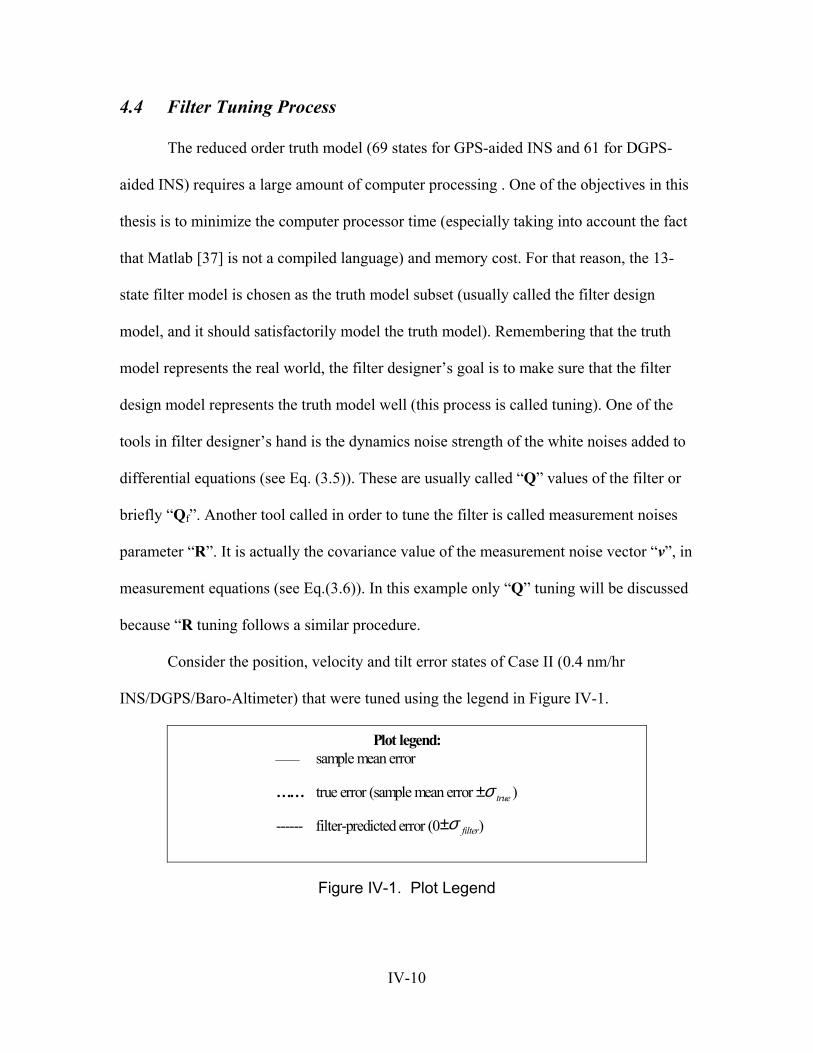
4.4 Filter Tuning Process
The reduced order truth model (69 states for GPS-aided INS and 61 for DGPS-
aided INS) requires a large amount of computer processing . One of the objectives in this
thesis is to minimize the computer processor time (especially taking into account the fact
that Matlab [37] is not a compiled language) and memory cost. For that reason, the 13-
state filter model is chosen as the truth model subset (usually called the filter design
model, and it should satisfactorily model the truth model). Remembering that the truth
model represents the real world, the filter designer’s goal is to make sure that the filter
design model represents the truth model well (this process is called tuning). One of the
tools in filter designer’s hand is the dynamics noise strength of the white noises added to
differential equations (see Eq. (3.5)). These are usually called “Q” values of the filter or
briefly “Qf”. Another tool called in order to tune the filter is called measurement noises
parameter “R”. It is actually the covariance value of the measurement noise vector “v”, in
measurement equations (see Eq.(3.6)). In this example only “Q” tuning will be discussed
because “R tuning follows a similar procedure.
Consider the position, velocity and tilt error states of Case II (0.4 nm/hr
INS/DGPS/Baro-Altimeter) that were tuned using the legend in Figure IV-1.
Plot legend:sample mean error
…… true error (sample mean error )
------ filter-predicted error (0 )
trueσ±
filterσ±
Figure IV-1. Plot Legend
IV-10
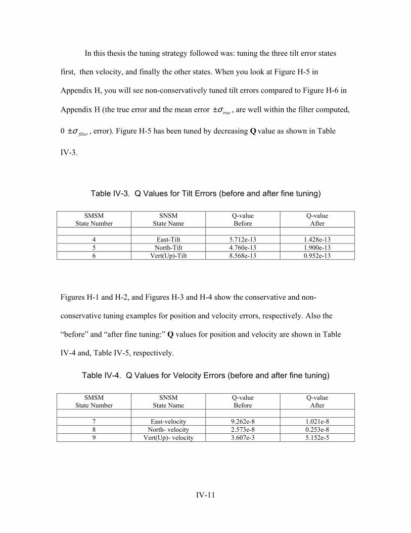
In this thesis the tuning strategy followed was: tuning the three tilt error states
first, then velocity, and finally the other states. When you look at Figure H-5 in
Appendix H, you will see non-conservatively tuned tilt errors compared to Figure H-6 in
Appendix H (the true error and the mean error , are well within the filter computed,
0
trueσ±
filterσ± , error). Figure H-5 has been tuned by decreasing Q value as shown in Table
IV-3.
Table IV-3. Q Values for Tilt Errors (before and after fine tuning)
SMSM State Number
SNSM State Name
Q-value Before
Q-value After
4 East-Tilt 5.712e-13 1.428e-13 5 North-Tilt 4.760e-13 1.900e-13 6 Vert(Up)-Tilt 8.568e-13 0.952e-13
Figures H-1 and H-2, and Figures H-3 and H-4 show the conservative and non-
conservative tuning examples for position and velocity errors, respectively. Also the
“before” and “after fine tuning:” Q values for position and velocity are shown in Table
IV-4 and, Table IV-5, respectively.
Table IV-4. Q Values for Velocity Errors (before and after fine tuning)
SMSM State Number
SNSM State Name
Q-value Before
Q-value After
7 East-velocity 9.262e-8 1.021e-8 8 North- velocity 2.573e-8 0.253e-8 9 Vert(Up)- velocity 3.607e-3 5.152e-5
IV-11
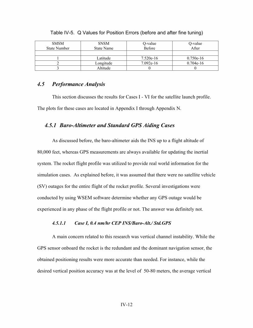
Table IV-5. Q Values for Position Errors (before and after fine tuning)
SMSM State Number
SNSM State Name
Q-value Before
Q-value After
1 Latitude 7.520e-16 0.750e-16 2 Longitude 7.092e-16 0.704e-16 3 Altitude 0 0
4.5 Performance Analysis
This section discusses the results for Cases I - VI for the satellite launch profile.
The plots for these cases are located in Appendix I through Appendix N.
4.5.1 Baro-Altimeter and Standard GPS Aiding Cases
As discussed before, the baro-altimeter aids the INS up to a flight altitude of
80,000 feet, whereas GPS measurements are always available for updating the inertial
system. The rocket flight profile was utilized to provide real world information for the
simulation cases. As explained before, it was assumed that there were no satellite vehicle
(SV) outages for the entire flight of the rocket profile. Several investigations were
conducted by using WSEM software determine whether any GPS outage would be
experienced in any phase of the flight profile or not. The answer was definitely not.
4.5.1.1 Case I, 0.4 nm/hr CEP INS/Baro-Alt./ Std.GPS
A main concern related to this research was vertical channel instability. While the
GPS sensor onboard the rocket is the redundant and the dominant navigation sensor, the
obtained positioning results were more accurate than needed. For instance, while the
desired vertical position accuracy was at the level of 50-80 meters, the average vertical
IV-12
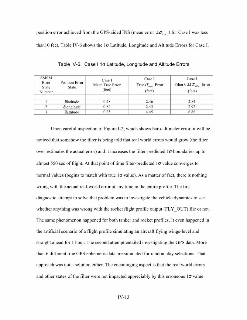
position error achieved from the GPS-aided INS (mean error ± ) for Case I was less
than10 feet. Table IV-6 shows the 1σ Latitude, Longitude and Altitude Errors for Case I.
trueσ
Table IV-6. Case I 1σ Latitude, Longitude and Altitude Errors
SMSM Error State
Number
Position Error State
Case I Mean True Error
(feet)
Case I True Error trueσ
(feet)
Case I Filter 0 1 filterσ± Error
(feet)
1 δlatitude 0.48 2.46 2.84 2 δlongitude 0.84 2.45 2.92 3 δaltitude 0.25 4.45 6.86
Upon careful inspection of Figure I-2, which shows baro-altimeter error, it will be
noticed that somehow the filter is being told that real world errors would grow (the filter
over-estimates the actual error) and it increases the filter-predicted 1σ boundaries up to
almost 550 sec of flight. At that point of time filter-predicted 1σ value converges to
normal values (begins to match with true 1σ value). As a matter of fact, there is nothing
wrong with the actual real-world error at any time in the entire profile. The first
diagnostic attempt to solve that problem was to investigate the vehicle dynamics to see
whether anything was wrong with the rocket flight profile output (FLY_OUT) file or not.
The same phenomenon happened for both tanker and rocket profiles. It even happened in
the artificial scenario of a flight profile simulating an aircraft flying wings-level and
straight ahead for 1 hour. The second attempt entailed investigating the GPS data. More
than 6 different true GPS ephemeris data are simulated for random day selections. That
approach was not a solution either. The encouraging aspect is that the real world errors
and other states of the filter were not impacted appreciably by this erroneous 1σ value
IV-13
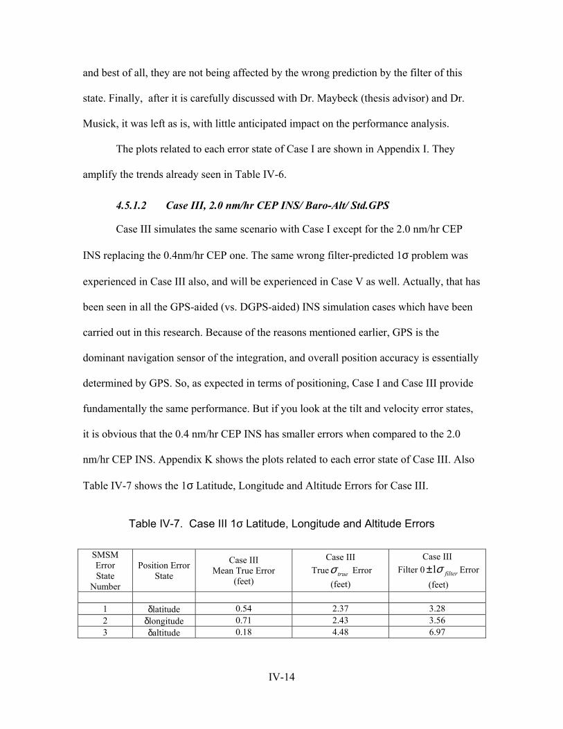
and best of all, they are not being affected by the wrong prediction by the filter of this
state. Finally, after it is carefully discussed with Dr. Maybeck (thesis advisor) and Dr.
Musick, it was left as is, with little anticipated impact on the performance analysis.
The plots related to each error state of Case I are shown in Appendix I. They
amplify the trends already seen in Table IV-6.
4.5.1.2 Case III, 2.0 nm/hr CEP INS/ Baro-Alt/ Std.GPS
Case III simulates the same scenario with Case I except for the 2.0 nm/hr CEP
INS replacing the 0.4nm/hr CEP one. The same wrong filter-predicted 1σ problem was
experienced in Case III also, and will be experienced in Case V as well. Actually, that has
been seen in all the GPS-aided (vs. DGPS-aided) INS simulation cases which have been
carried out in this research. Because of the reasons mentioned earlier, GPS is the
dominant navigation sensor of the integration, and overall position accuracy is essentially
determined by GPS. So, as expected in terms of positioning, Case I and Case III provide
fundamentally the same performance. But if you look at the tilt and velocity error states,
it is obvious that the 0.4 nm/hr CEP INS has smaller errors when compared to the 2.0
nm/hr CEP INS. Appendix K shows the plots related to each error state of Case III. Also
Table IV-7 shows the 1σ Latitude, Longitude and Altitude Errors for Case III.
Table IV-7. Case III 1σ Latitude, Longitude and Altitude Errors
SMSM Error State
Number
Position Error State
Case III Mean True Error
(feet)
Case III True Error trueσ
(feet)
Case III Filter 0 1 filterσ± Error
(feet)
1 δlatitude 0.54 2.37 3.28 2 δlongitude 0.71 2.43 3.56 3 δaltitude 0.18 4.48 6.97
IV-14
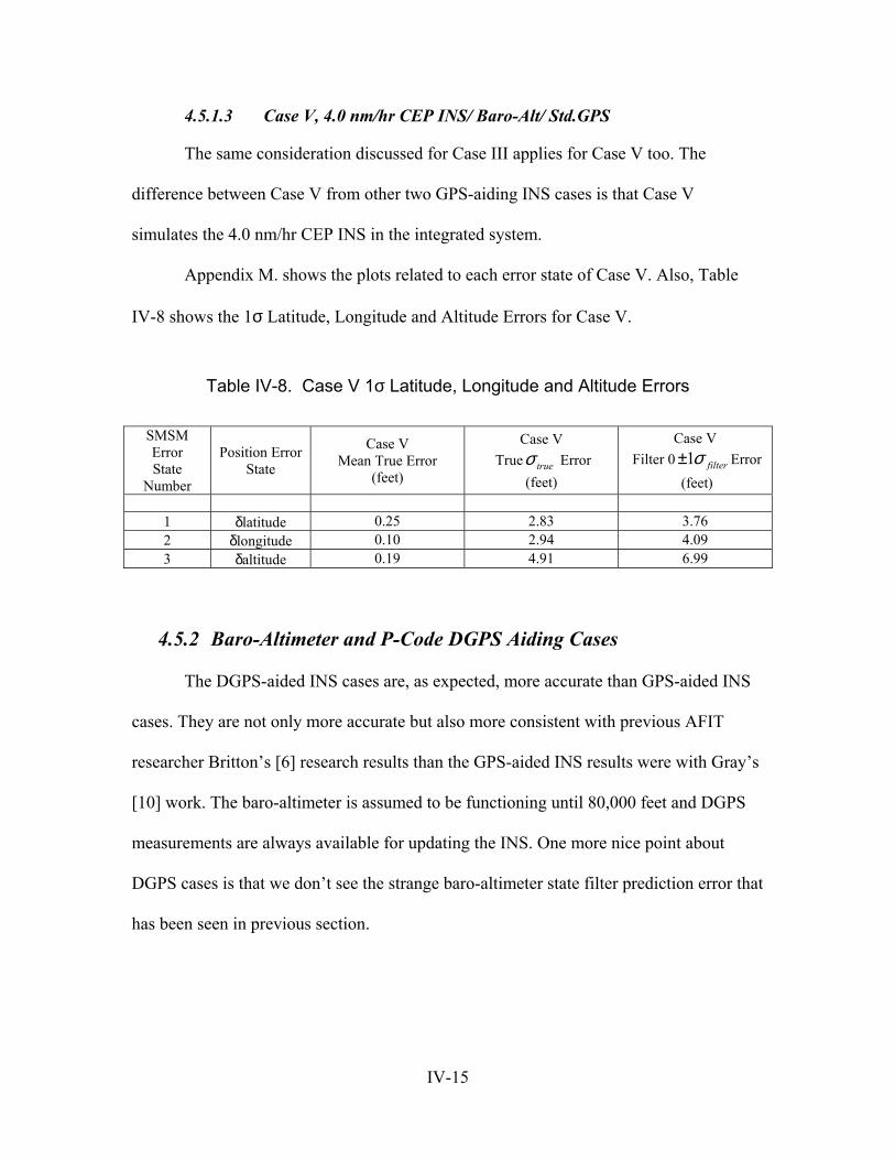
4.5.1.3 Case V, 4.0 nm/hr CEP INS/ Baro-Alt/ Std.GPS
The same consideration discussed for Case III applies for Case V too. The
difference between Case V from other two GPS-aiding INS cases is that Case V
simulates the 4.0 nm/hr CEP INS in the integrated system.
Appendix M. shows the plots related to each error state of Case V. Also, Table
IV-8 shows the 1σ Latitude, Longitude and Altitude Errors for Case V.
Table IV-8. Case V 1σ Latitude, Longitude and Altitude Errors
SMSM Error State
Number
Position Error State
Case V Mean True Error
(feet)
Case V True Error trueσ
(feet)
Case V Filter 0 1 filterσ± Error
(feet)
1 δlatitude 0.25 2.83 3.76 2 δlongitude 0.10 2.94 4.09 3 δaltitude 0.19 4.91 6.99
4.5.2 Baro-Altimeter and P-Code DGPS Aiding Cases
The DGPS-aided INS cases are, as expected, more accurate than GPS-aided INS
cases. They are not only more accurate but also more consistent with previous AFIT
researcher Britton’s [6] research results than the GPS-aided INS results were with Gray’s
[10] work. The baro-altimeter is assumed to be functioning until 80,000 feet and DGPS
measurements are always available for updating the INS. One more nice point about
DGPS cases is that we don’t see the strange baro-altimeter state filter prediction error that
has been seen in previous section.
IV-15
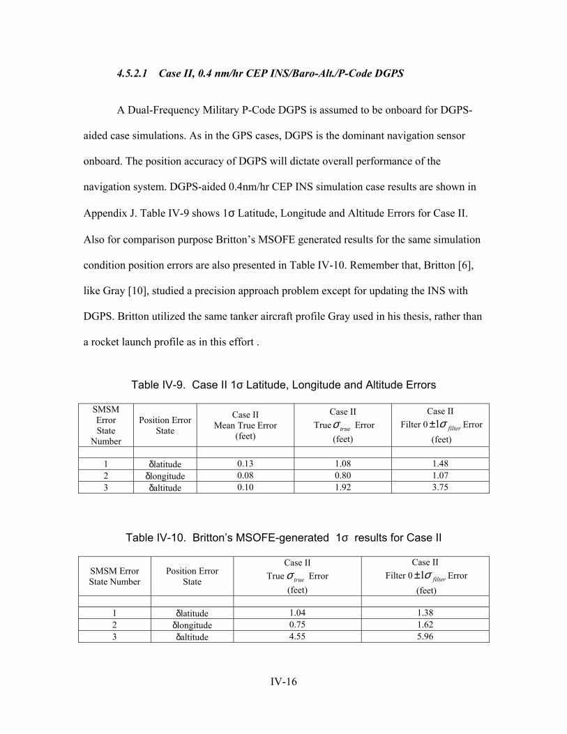
4.5.2.1 Case II, 0.4 nm/hr CEP INS/Baro-Alt./P-Code DGPS
A Dual-Frequency Military P-Code DGPS is assumed to be onboard for DGPS-
aided case simulations. As in the GPS cases, DGPS is the dominant navigation sensor
onboard. The position accuracy of DGPS will dictate overall performance of the
navigation system. DGPS-aided 0.4nm/hr CEP INS simulation case results are shown in
Appendix J. Table IV-9 shows 1σ Latitude, Longitude and Altitude Errors for Case II.
Also for comparison purpose Britton’s MSOFE generated results for the same simulation
condition position errors are also presented in Table IV-10. Remember that, Britton [6],
like Gray [10], studied a precision approach problem except for updating the INS with
DGPS. Britton utilized the same tanker aircraft profile Gray used in his thesis, rather than
a rocket launch profile as in this effort .
Table IV-9. Case II 1σ Latitude, Longitude and Altitude Errors
SMSM Error State
Number
Position Error State
Case II Mean True Error
(feet)
Case II True Error trueσ
(feet)
Case II Filter 0 1 filterσ± Error
(feet)
1 δlatitude 0.13 1.08 1.48 2 δlongitude 0.08 0.80 1.07 3 δaltitude 0.10 1.92 3.75
Table IV-10. Britton’s MSOFE-generated 1σ results for Case II
SMSM Error State Number
Position Error State
Case II True Error trueσ
(feet)
Case II Filter 0 1 filterσ± Error
(feet)
1 δlatitude 1.04 1.38 2 δlongitude 0.75 1.62 3 δaltitude 4.55 5.96
IV-16
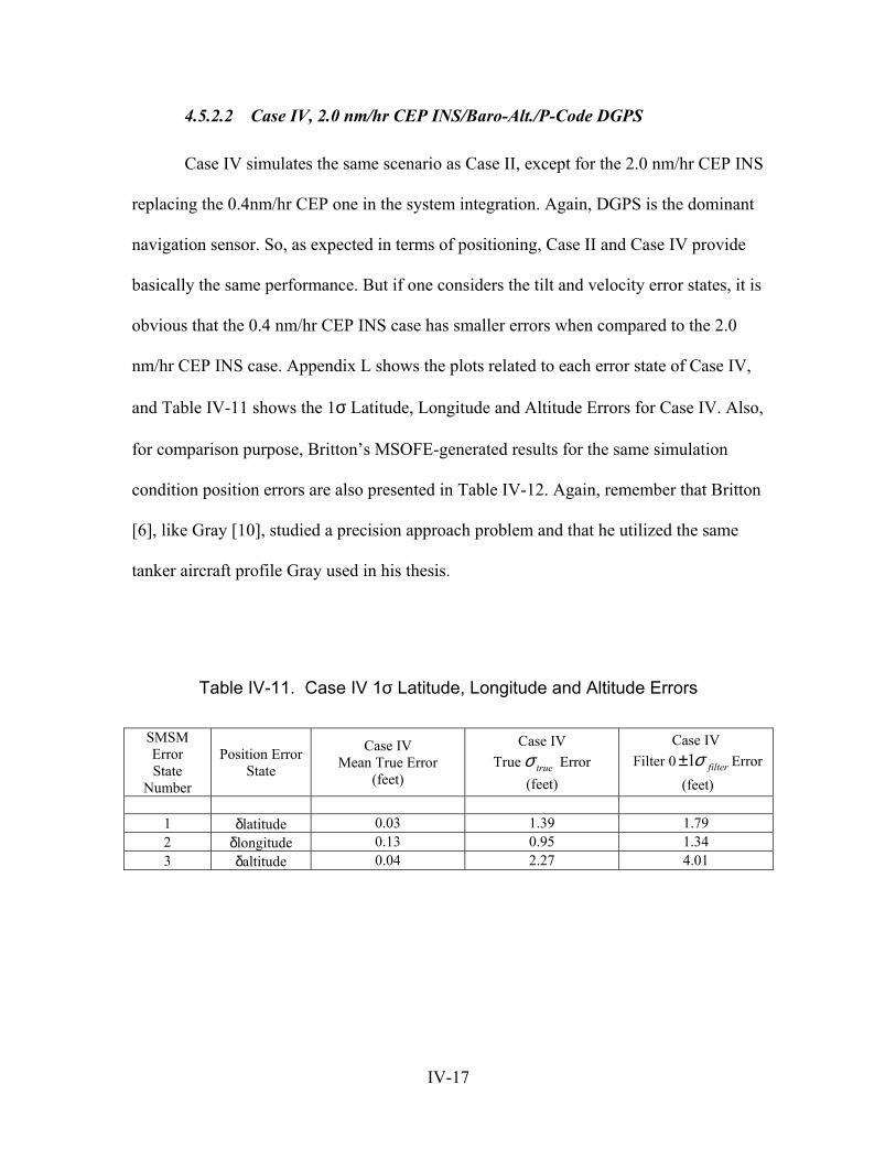
4.5.2.2 Case IV, 2.0 nm/hr CEP INS/Baro-Alt./P-Code DGPS
Case IV simulates the same scenario as Case II, except for the 2.0 nm/hr CEP INS
replacing the 0.4nm/hr CEP one in the system integration. Again, DGPS is the dominant
navigation sensor. So, as expected in terms of positioning, Case II and Case IV provide
basically the same performance. But if one considers the tilt and velocity error states, it is
obvious that the 0.4 nm/hr CEP INS case has smaller errors when compared to the 2.0
nm/hr CEP INS case. Appendix L shows the plots related to each error state of Case IV,
and Table IV-11 shows the 1σ Latitude, Longitude and Altitude Errors for Case IV. Also,
for comparison purpose, Britton’s MSOFE-generated results for the same simulation
condition position errors are also presented in Table IV-12. Again, remember that Britton
[6], like Gray [10], studied a precision approach problem and that he utilized the same
tanker aircraft profile Gray used in his thesis.
Table IV-11. Case IV 1σ Latitude, Longitude and Altitude Errors
SMSM Error State
Number
Position Error State
Case IV Mean True Error
(feet)
Case IV True Error trueσ
(feet)
Case IV Filter 0 1 filterσ± Error
(feet)
1 δlatitude 0.03 1.39 1.79 2 δlongitude 0.13 0.95 1.34 3 δaltitude 0.04 2.27 4.01
IV-17
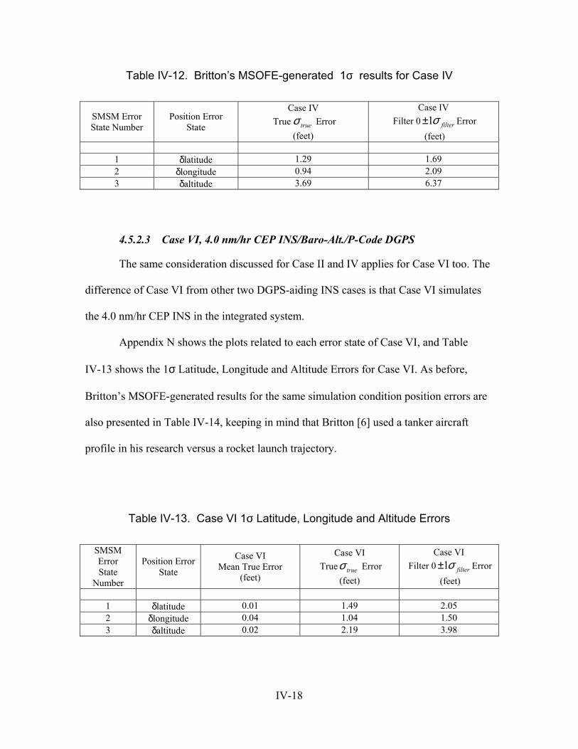
Table IV-12. Britton’s MSOFE-generated 1σ results for Case IV
SMSM Error State Number
Position Error State
Case IV True Error trueσ
(feet)
Case IV Filter 0 1 filterσ± Error
(feet)
1 δlatitude 1.29 1.69 2 δlongitude 0.94 2.09 3 δaltitude 3.69 6.37
4.5.2.3 Case VI, 4.0 nm/hr CEP INS/Baro-Alt./P-Code DGPS
The same consideration discussed for Case II and IV applies for Case VI too. The
difference of Case VI from other two DGPS-aiding INS cases is that Case VI simulates
the 4.0 nm/hr CEP INS in the integrated system.
Appendix N shows the plots related to each error state of Case VI, and Table
IV-13 shows the 1σ Latitude, Longitude and Altitude Errors for Case VI. As before,
Britton’s MSOFE-generated results for the same simulation condition position errors are
also presented in Table IV-14, keeping in mind that Britton [6] used a tanker aircraft
profile in his research versus a rocket launch trajectory.
Table IV-13. Case VI 1σ Latitude, Longitude and Altitude Errors
SMSM Error State
Number
Position Error State
Case VI Mean True Error
(feet)
Case VI True Error trueσ
(feet)
Case VI Filter 0 1 filterσ± Error
(feet)
1 δlatitude 0.01 1.49 2.05 2 δlongitude 0.04 1.04 1.50 3 δaltitude 0.02 2.19 3.98
IV-18
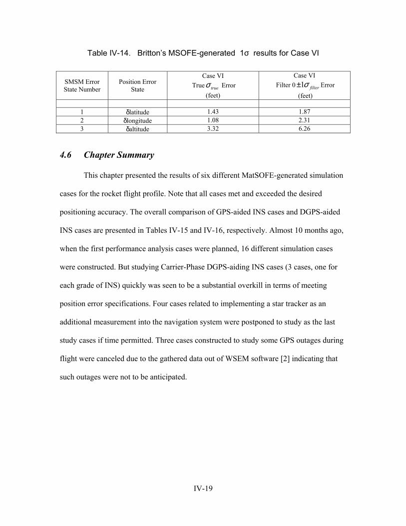
Table IV-14. Britton’s MSOFE-generated 1σ results for Case VI
SMSM Error State Number
Position Error State
Case VI True Error trueσ
(feet)
Case VI Filter 0 1 filterσ± Error
(feet)
1 δlatitude 1.43 1.87 2 δlongitude 1.08 2.31 3 δaltitude 3.32 6.26
4.6 Chapter Summary
This chapter presented the results of six different MatSOFE-generated simulation
cases for the rocket flight profile. Note that all cases met and exceeded the desired
positioning accuracy. The overall comparison of GPS-aided INS cases and DGPS-aided
INS cases are presented in Tables IV-15 and IV-16, respectively. Almost 10 months ago,
when the first performance analysis cases were planned, 16 different simulation cases
were constructed. But studying Carrier-Phase DGPS-aiding INS cases (3 cases, one for
each grade of INS) quickly was seen to be a substantial overkill in terms of meeting
position error specifications. Four cases related to implementing a star tracker as an
additional measurement into the navigation system were postponed to study as the last
study cases if time permitted. Three cases constructed to study some GPS outages during
flight were canceled due to the gathered data out of WSEM software [2] indicating that
such outages were not to be anticipated.
IV-19
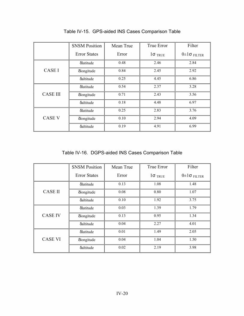
Table IV-15. GPS-aided INS Cases Comparison Table
SNSM Position
Error States
Mean True
Error
True Error
1σ TRUE
Filter
0±1σ FILTER
δlatitude 0.48 2.46 2.84
δlongitude 0.84 2.45 2.92 CASE I
δaltitude 0.25 4.45 6.86
δlatitude 0.54 2.37 3.28
δlongitude 0.71 2.43 3.56 CASE III
δaltitude 0.18 4.48 6.97
δlatitude 0.25 2.83 3.76
δlongitude 0.10 2.94 4.09 CASE V
δaltitude 0.19 4.91 6.99
Table IV-16. DGPS-aided INS Cases Comparison Table
SNSM Position
Error States
Mean True
Error
True Error
1σ TRUE
Filter
0±1σ FILTER
δlatitude 0.13 1.08 1.48
δlongitude 0.08 0.80 1.07 CASE II
δaltitude 0.10 1.92 3.75
δlatitude 0.03 1.39 1.79
δlongitude 0.13 0.95 1.34 CASE IV
δaltitude 0.04 2.27 4.01
δlatitude 0.01 1.49 2.05
δlongitude 0.04 1.04 1.50 CASE VI
δaltitude 0.02 2.19 3.98
IV-20
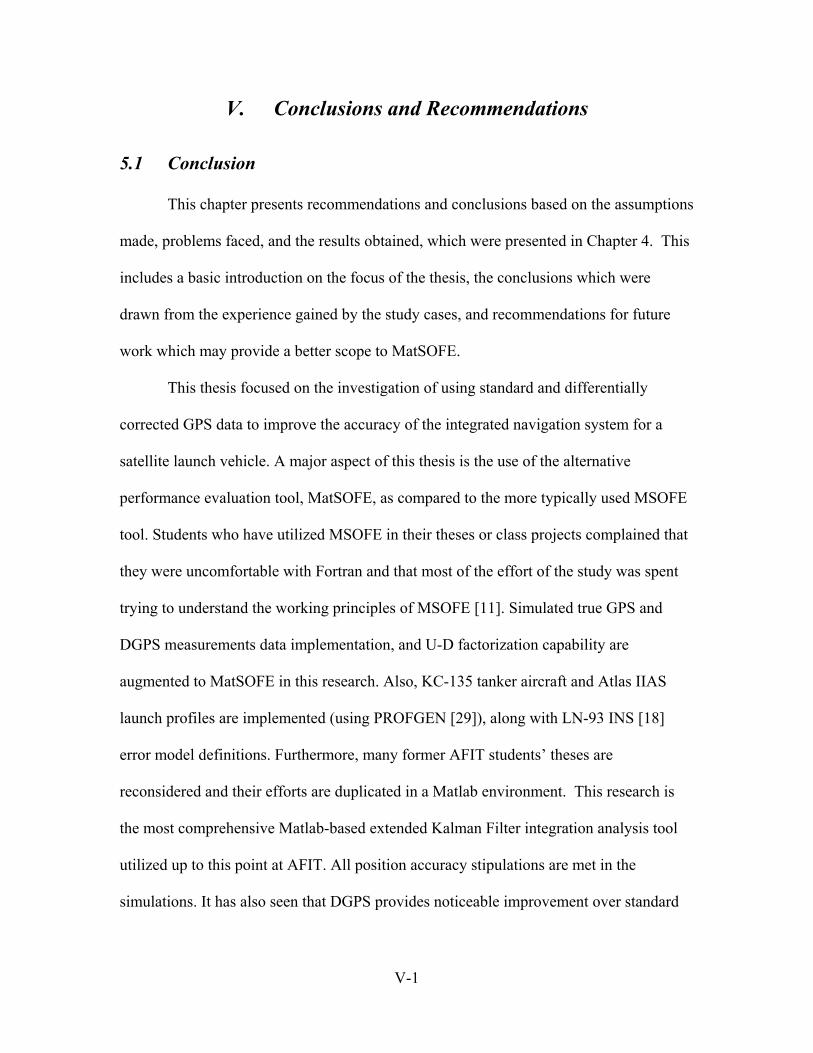
V. Conclusions and Recommendations
5.1 Conclusion
This chapter presents recommendations and conclusions based on the assumptions
made, problems faced, and the results obtained, which were presented in Chapter 4. This
includes a basic introduction on the focus of the thesis, the conclusions which were
drawn from the experience gained by the study cases, and recommendations for future
work which may provide a better scope to MatSOFE.
This thesis focused on the investigation of using standard and differentially
corrected GPS data to improve the accuracy of the integrated navigation system for a
satellite launch vehicle. A major aspect of this thesis is the use of the alternative
performance evaluation tool, MatSOFE, as compared to the more typically used MSOFE
tool. Students who have utilized MSOFE in their theses or class projects complained that
they were uncomfortable with Fortran and that most of the effort of the study was spent
trying to understand the working principles of MSOFE [11]. Simulated true GPS and
DGPS measurements data implementation, and U-D factorization capability are
augmented to MatSOFE in this research. Also, KC-135 tanker aircraft and Atlas IIAS
launch profiles are implemented (using PROFGEN [29]), along with LN-93 INS [18]
error model definitions. Furthermore, many former AFIT students’ theses are
reconsidered and their efforts are duplicated in a Matlab environment. This research is
the most comprehensive Matlab-based extended Kalman Filter integration analysis tool
utilized up to this point at AFIT. All position accuracy stipulations are met in the
simulations. It has also seen that DGPS provides noticeable improvement over standard
V-1
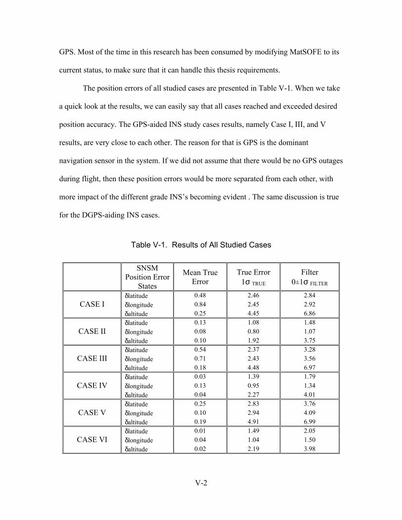
GPS. Most of the time in this research has been consumed by modifying MatSOFE to its
current status, to make sure that it can handle this thesis requirements.
The position errors of all studied cases are presented in Table V-1. When we take
a quick look at the results, we can easily say that all cases reached and exceeded desired
position accuracy. The GPS-aided INS study cases results, namely Case I, III, and V
results, are very close to each other. The reason for that is GPS is the dominant
navigation sensor in the system. If we did not assume that there would be no GPS outages
during flight, then these position errors would be more separated from each other, with
more impact of the different grade INS’s becoming evident . The same discussion is true
for the DGPS-aiding INS cases.
Table V-1. Results of All Studied Cases
SNSM
Position Error States
True Error 1σ
Filter 0±1σ FILTER
Mean True Error TRUE
0.48 2.46 2.84 δlatitude δlongitude 0.84 2.45 2.92 CASE I δaltitude 0.25 4.45 6.86 δlatitude 0.13 1.08 1.48 δlongitude 0.08 0.80 1.07 CASE II δaltitude 0.10 1.92 3.75 δlatitude 0.54 2.37 3.28 δlongitude 0.71 2.43 3.56 CASE III δaltitude 0.18 4.48 6.97 δlatitude 0.03 1.39 1.79 δlongitude 0.13 0.95 1.34 CASE IV δaltitude 0.04 2.27 4.01 δlatitude 0.25 2.83 3.76 δlongitude 0.10 2.94 4.09 CASE V δaltitude 0.19 4.91 6.99 δlatitude 0.01 1.49 2.05 δlongitude 0.04 1.04 1.50 CASE VI δaltitude 0.02 2.19 3.98
V-2
5.2 Recommendations
This thesis has started with examining the work Gray [10] and Britton [6]
accomplished. Their achievements for GPS and DGPS integrated extended Kalman filter
integrations are considered as the bases of this research.
•
•
•
•
•
MatSOFE is written without any access to MSOFE. Therefore, it is believed
by the author that, as a future effort MatSOFE can be made more reliable and
robust Kalman filter evaluation tool, as opposed to current capabilities it has.
The real emphasis on this research was position accuracy, and it has seen that
the problem related to baro-altimeter error state has no appreciable impact on
other error states. It is also believed that this phenomenon could be a result of
not being able to see the original MSOFE code.
The INS performance is a little bit disregarded since no GPS outage during
flight was one of the assumptions and GPS accuracy is superior over INS.
It was not necessary for this thesis, but for future usage, carrier-phase GPS
signals can be implemented to increase the accuracy of the GPS
measurements to the centimeter level for necessary navigation problems. A
viable carrier-phase model was not available for the MatSOFE package during
this study. If time allowed, developing and utilizing such an accurate
measurement system, would, perhaps make MatSOFE one of the best and
most versatile performance evaluation tools available.
According to reviewed literature, the navigation sensor used in Atlas IIAS is
only INS [15]. Also, there are some other launch vehicles using GPS-aided
INS navigation system. At the very beginning of this study, it was quite clear
V-3
that even the worst case of this study (CASE I, GPS-aided 0.4 nm/hr CEP
INS) would meet and exceed the position requirements. The only reason for
incorporating DGPS measurements into system was to make MatSOFE a
more useful and reliable filter performance evaluation tool in the future. In
reality incorporating DGPS measurements would not be enough. The
reference receiver positioning and means of differential corrections should
also be included inside the research scope, but this was not pursued here
because of the good non-differential GPS-aided INS performance.
V-4
Appendix A Error State Definitions for the SNSM Truth and Filter Models
Tabular listings of the truth and filter models are presented. Tables A-1 and A-2
show the 39 INS states for the truth model, with the SNU 84-1 [Litton,18] and LSM [10]
and DLSM [6] state numbers given for cross-reference. Table A-3 lists the GPS states
and Table A-4 lists DGPS states respectively, and finally Table A-5 lists the states in the
reduced-ordered SNSM filter model.
A- 1
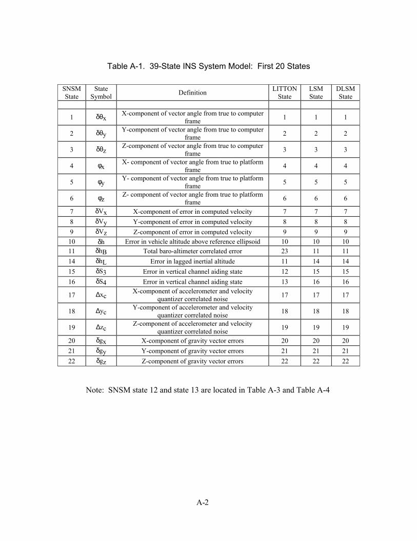
Table A-1. 39-State INS System Model: First 20 States
SNSM State
State Symbol Definition LITTON
State LSM State
DLSM State
1 δθx X-component of vector angle from true to computer frame 1 1 1
2 δθy Y-component of vector angle from true to computer frame 2 2 2
3 δθz Z-component of vector angle from true to computer frame 3 3 3
4 φx X- component of vector angle from true to platform frame 4 4 4
5 φy Y- component of vector angle from true to platform frame 5 5 5
6 φz Z- component of vector angle from true to platform frame 6 6 6
7 δVx X-component of error in computed velocity 7 7 7 8 δVy Y-component of error in computed velocity 8 8 8 9 δVz Z-component of error in computed velocity 9 9 9
10 δh Error in vehicle altitude above reference ellipsoid 10 10 10 11 δhB Total baro-altimeter correlated error 23 11 11 14 δhL Error in lagged inertial altitude 11 14 14 15 δS3 Error in vertical channel aiding state 12 15 15 16 δS4 Error in vertical channel aiding state 13 16 16
17 ∆xc X-component of accelerometer and velocity quantizer correlated noise 17 17 17
18 ∆yc Y-component of accelerometer and velocity quantizer correlated noise 18 18 18
19 ∆zc Z-component of accelerometer and velocity quantizer correlated noise 19 19 19
20 δgx X-component of gravity vector errors 20 20 20 21 δgy Y-component of gravity vector errors 21 21 21 22 δgz Z-component of gravity vector errors 22 22 22
Note: SNSM state 12 and state 13 are located in Table A-3 and Table A-4
A- 2
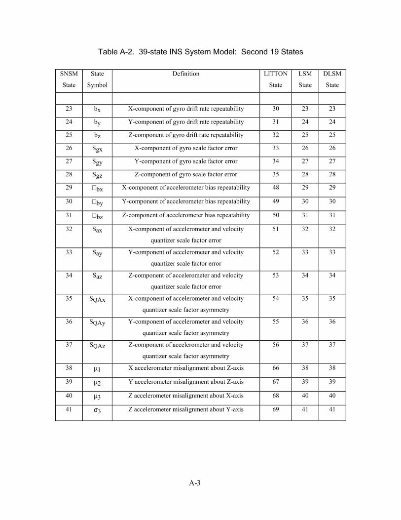
Table A-2. 39-state INS System Model: Second 19 States
SNSM
State
State
Symbol
Definition LITTON
State
LSM
State
DLSM
State
23 bx X-component of gyro drift rate repeatability 30 23 23
24 by Y-component of gyro drift rate repeatability 31 24 24
25 bz Z-component of gyro drift rate repeatability 32 25 25
26 Sgx X-component of gyro scale factor error 33 26 26
27 Sgy Y-component of gyro scale factor error 34 27 27
28 Sgz Z-component of gyro scale factor error 35 28 28
29 ∇ bx X-component of accelerometer bias repeatability 48 29 29
30 ∇ by Y-component of accelerometer bias repeatability 49 30 30
31 ∇ bz Z-component of accelerometer bias repeatability 50 31 31
32 Sax X-component of accelerometer and velocity
quantizer scale factor error
51 32 32
33 Say Y-component of accelerometer and velocity
quantizer scale factor error
52 33 33
34 Saz Z-component of accelerometer and velocity
quantizer scale factor error
53 34 34
35 SQAx X-component of accelerometer and velocity
quantizer scale factor asymmetry
54 35 35
36 SQAy Y-component of accelerometer and velocity
quantizer scale factor asymmetry
55 36 36
37 SQAz Z-component of accelerometer and velocity
quantizer scale factor asymmetry
56 37 37
38 µ1 X accelerometer misalignment about Z-axis 66 38 38
39 µ2 Y accelerometer misalignment about Z-axis 67 39 39
40 µ3 Z accelerometer misalignment about X-axis 68 40 40
41 σ3 Z accelerometer misalignment about Y-axis 69 41 41
A- 3
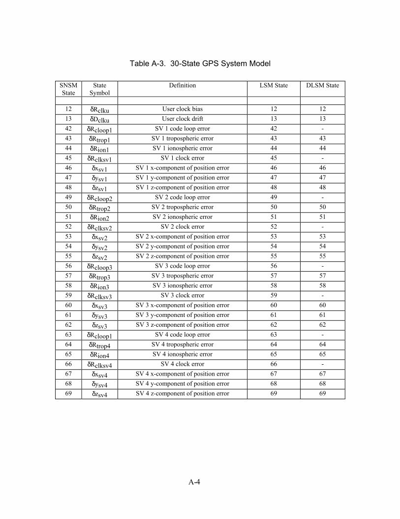
Table A-3. 30-State GPS System Model
SNSM State
State Symbol
Definition LSM State DLSM State
12 δRclku User clock bias 12 12 13 δDclku User clock drift 13 13 42 δRcloop1 SV 1 code loop error 42 - 43 δRtrop1 SV 1 tropospheric error 43 43 44 δRion1 SV 1 ionospheric error 44 44 45 δRclksv1 SV 1 clock error 45 - 46 δxsv1 SV 1 x-component of position error 46 46 47 δysv1 SV 1 y-component of position error 47 47 48 δzsv1 SV 1 z-component of position error 48 48 49 δRcloop2 SV 2 code loop error 49 - 50 δRtrop2 SV 2 tropospheric error 50 50 51 δRion2 SV 2 ionospheric error 51 51 52 δRclksv2 SV 2 clock error 52 - 53 δxsv2 SV 2 x-component of position error 53 53 54 δysv2 SV 2 y-component of position error 54 54 55 δzsv2 SV 2 z-component of position error 55 55 56 δRcloop3 SV 3 code loop error 56 - 57 δRtrop3 SV 3 tropospheric error 57 57 58 δRion3 SV 3 ionospheric error 58 58 59 δRclksv3 SV 3 clock error 59 - 60 δxsv3 SV 3 x-component of position error 60 60 61 δysv3 SV 3 y-component of position error 61 61 62 δzsv3 SV 3 z-component of position error 62 62 63 δRcloop1 SV 4 code loop error 63 - 64 δRtrop4 SV 4 tropospheric error 64 64 65 δRion4 SV 4 ionospheric error 65 65 66 δRclksv4 SV 4 clock error 66 - 67 δxsv4 SV 4 x-component of position error 67 67 68 δysv4 SV 4 y-component of position error 68 68 69 δzsv4 SV 4 z-component of position error 69 69
A- 4
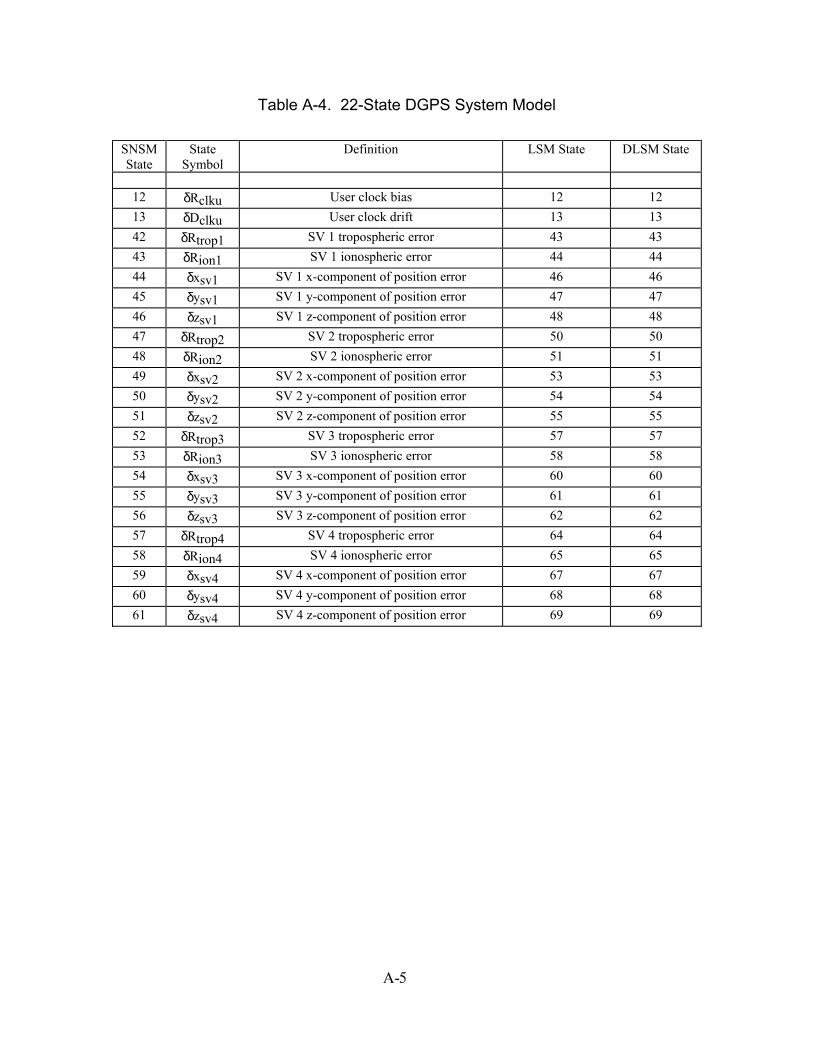
Table A-4. 22-State DGPS System Model
SNSM State
State Symbol
Definition LSM State DLSM State
12 δRclku User clock bias 12 12 13 δDclku User clock drift 13 13 42 δRtrop1 SV 1 tropospheric error 43 43 43 δRion1 SV 1 ionospheric error 44 44 44 δxsv1 SV 1 x-component of position error 46 46 45 δysv1 SV 1 y-component of position error 47 47 46 δzsv1 SV 1 z-component of position error 48 48 47 δRtrop2 SV 2 tropospheric error 50 50 48 δRion2 SV 2 ionospheric error 51 51 49 δxsv2 SV 2 x-component of position error 53 53 50 δysv2 SV 2 y-component of position error 54 54 51 δzsv2 SV 2 z-component of position error 55 55 52 δRtrop3 SV 3 tropospheric error 57 57 53 δRion3 SV 3 ionospheric error 58 58 54 δxsv3 SV 3 x-component of position error 60 60 55 δysv3 SV 3 y-component of position error 61 61 56 δzsv3 SV 3 z-component of position error 62 62 57 δRtrop4 SV 4 tropospheric error 64 64 58 δRion4 SV 4 ionospheric error 65 65 59 δxsv4 SV 4 x-component of position error 67 67 60 δysv4 SV 4 y-component of position error 68 68 61 δzsv4 SV 4 z-component of position error 69 69
A- 5
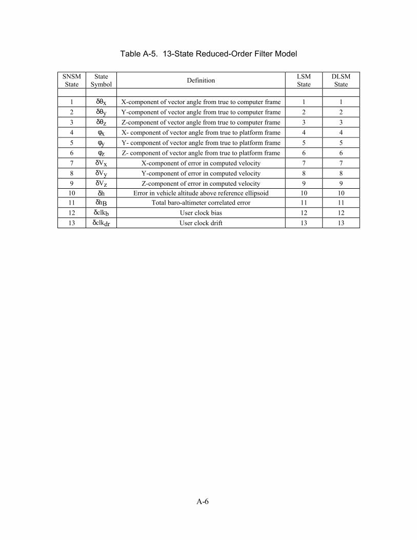
Table A-5. 13-State Reduced-Order Filter Model
SNSM State
State Symbol Definition LSM
State DLSM State
1 δθx X-component of vector angle from true to computer frame 1 1 2 δθy Y-component of vector angle from true to computer frame 2 2 3 δθz Z-component of vector angle from true to computer frame 3 3 4 φx X- component of vector angle from true to platform frame 4 4 5 φy Y- component of vector angle from true to platform frame 5 5 6 φz Z- component of vector angle from true to platform frame 6 6 7 δVx X-component of error in computed velocity 7 7 8 δVy Y-component of error in computed velocity 8 8 9 δVz Z-component of error in computed velocity 9 9
10 δh Error in vehicle altitude above reference ellipsoid 10 10 11 δhB Total baro-altimeter correlated error 11 11 12 δclkb User clock bias 12 12 13 δclkdr User clock drift 13 13
A- 6
Appendix B Dynamics Matrices and Noise Values
B.1 Definition of Dynamics Matrices
In Chapter 3, the truth and filter model dynamics are defined by the submatrices,
, , , , and FilterF1tINSF
2tINSFtGPSF
tDGPSF of Equation (3.5). The F represents the filter
dynamics matrix, which is also a submatrix of the larger truth model dynamics matrix
[27]. The other three matrices represent the additional truth model non-zero portions of
the F matrix that simulate the real world [27,33]. Tables B-2, B-3, B-4, B-5, and B-6
contain the non-zero elements of the dynamics submatrices F , F , F , F ,
and
Filter
Filter 1tINS 2tINS tGPS
tDGPSF , respectively. All undeclared variables shown in the following tables are
defined in the LN-93 technical report, along with their units [18,27]. The structure of the
dynamics matrices in this chapter correspond to the truth model state definitions in
Appendix A and to the AFIT thesis (LSM/DLSM model) by [6,10]. The notation used in
Table B-2 through Table B-4in this Appendix is defined in Table B-1.
B- 1
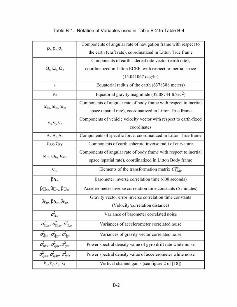
Table B-1. Notation of Variables used in Table B-2 to Table B-4
ρx, ρy, ρz Components of angular rate of navigation frame with respect to
the earth (craft rate), coordinatized in Litton True frame
Ωx, Ωy, Ωz
Components of earth sidereal rate vector (earth rate),
coordinatized in Litton ECEF, with respect to inertial space
(15.041067 deg/hr)
a Equatorial radius of the earth (6378388 meters)
go Equatorial gravity magnitude (32.08744 ft/sec2)
ωitx, ωity, ωitz Components of angular rate of body frame with respect to inertial
space (spatial rate), coordinatized in Litton True frame
Vx,Vy,Vz Components of vehicle velocity vector with respect to earth-fixed
coordinates
Ax, Ay, Az Components of specific force, coordinatized in Litton True frame
CRX, CRY Components of earth spheroid inverse radii of curvature
ωibx, ωiby, ωibz Components of angular rate of body frame with respect to inertial
space (spatial rate), coordinatized in Litton Body frame
Ci,j Elements of the transformation matrix C bodynav
βδhc Barometer inverse correlation time (600 seconds)
β∇ xc, β∇ yc, β∇ zc Accelerometer inverse correlation time constants (5 minutes)
βδgx, βδgy, βδgz Gravity vector error inverse correlation time constants
(Velocity/correlation distance)
σδhc2 Variance of barometer correlated noise
σ∇ xc2 , , σ∇ yc
2 σ∇ zc2 Variances of accelerometer correlated noise
σδgx2 , , σδgy
2 σδgz2 Variances of gravity vector correlated noise
σηbx2 , , σηby
2 σηbz2 Power spectral density value of gyro drift rate white noise
σηAx2 , , σηAy
2 σηAz2 Power spectral density value of accelerometer white noise
k1, k2, k3, k4 Vertical channel gains (see figure 2 of [18])
B- 2
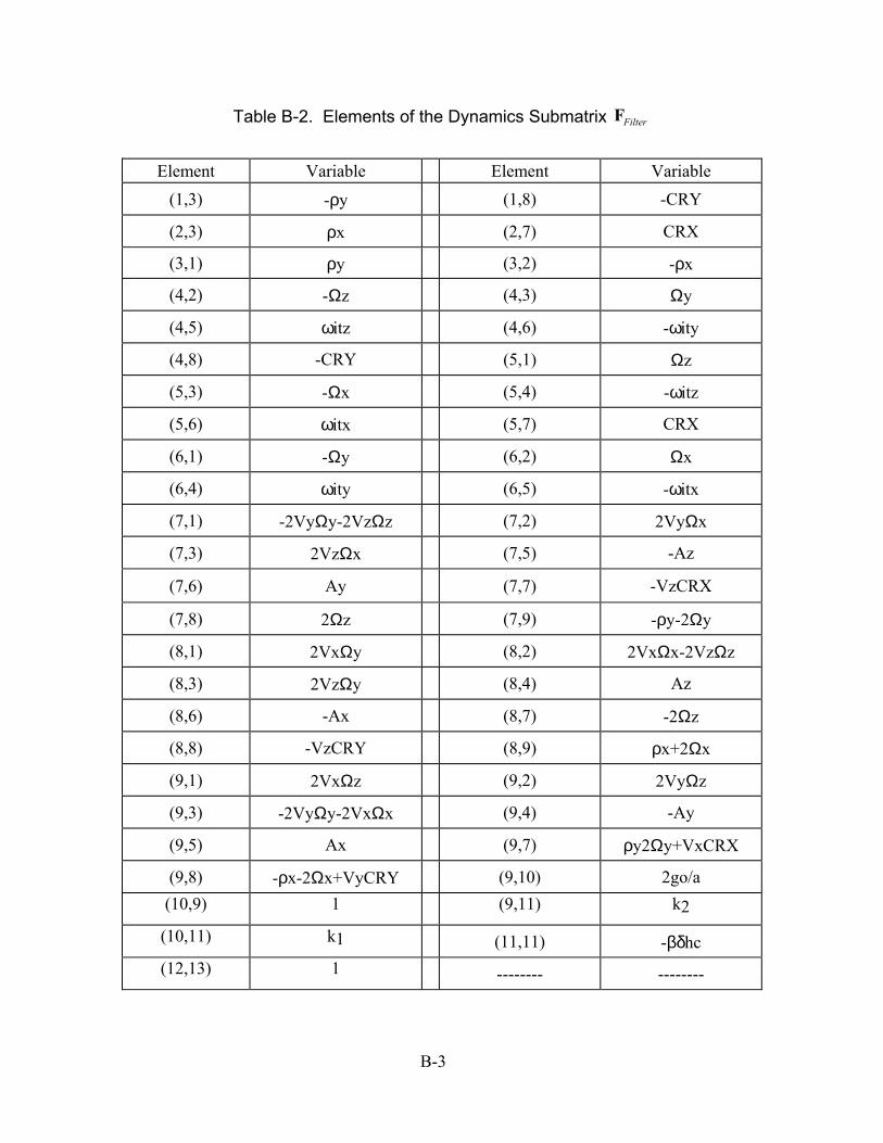
Table B-2. Elements of the Dynamics Submatrix FilterF
Element Variable Element Variable (1,3) -ρy (1,8) -CRY
(2,3) ρx (2,7) CRX
(3,1) ρy (3,2) -ρx
(4,2) -Ωz (4,3) Ωy
(4,5) ωitz (4,6) -ωity
(4,8) -CRY (5,1) Ωz
(5,3) -Ωx (5,4) -ωitz
(5,6) ωitx (5,7) CRX
(6,1) -Ωy (6,2) Ωx
(6,4) ωity (6,5) -ωitx
(7,1) -2VyΩy-2VzΩz (7,2) 2VyΩx
(7,3) 2VzΩx (7,5) -Az
(7,6) Ay (7,7) -VzCRX
(7,8) 2Ωz (7,9) -ρy-2Ωy
(8,1) 2VxΩy (8,2) 2VxΩx-2VzΩz
(8,3) 2VzΩy (8,4) Az
(8,6) -Ax (8,7) -2Ωz
(8,8) -VzCRY (8,9) ρx+2Ωx
(9,1) 2VxΩz (9,2) 2VyΩz
(9,3) -2VyΩy-2VxΩx (9,4) -Ay
(9,5) Ax (9,7) ρy2Ωy+VxCRX
(9,8) -ρx-2Ωx+VyCRY (9,10) 2go/a (10,9) 1 (9,11) k2
(10,11) k1 (11,11) -βδhc (12,13) 1 -------- --------
B- 3
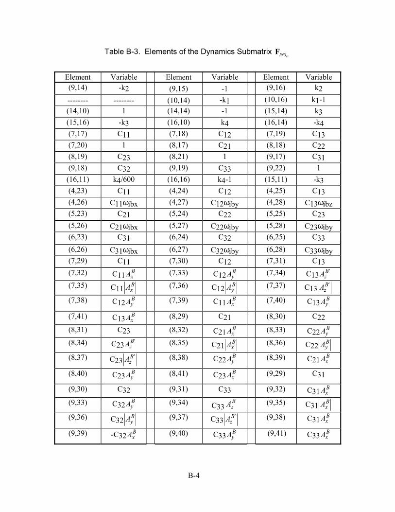
Table B-3. Elements of the Dynamics Submatrix 1tINSF
Element Variable Element Variable Element Variable (9,14) -k2 (9,15) -1 (9,16) k2
-------- -------- (10,14) -k1 (10,16) k1-1 (14,10) 1 (14,14) -1 (15,14) k3 (15,16) -k3 (16,10) k4 (16,14) -k4 (7,17) C11 (7,18) C12 (7,19) C13 (7,20) 1 (8,17) C21 (8,18) C22 (8,19) C23 (8,21) 1 (9,17) C31 (9,18) C32 (9,19) C33 (9,22) 1 (16,11) k4/600 (16,16) k4-1 (15,11) -k3 (4,23) C11 (4,24) C12 (4,25) C13 (4,26) C11ωibx (4,27) C12ωiby (4,28) C13ωibz (5,23) C21 (5,24) C22 (5,25) C23 (5,26) C21ωibx (5,27) C22ωiby (5,28) C23ωiby (6,23) C31 (6,24) C32 (6,25) C33 (6,26) C31ωibx (6,27) C32ωiby (6,28) C33ωiby (7,29) C11 (7,30) C12 (7,31) C13 (7,32) C11 Ax
B (7,33) C12 AyB (7,34) C13 Az
B′ (7,35) C11 Ax
B (7,36) C12 AyB (7,37) C13 Az
B′
(7,38) C12 AyB (7,39) C11 Ax
B (7,40) C13 AyB
(7,41) C13 AxB (8,29) C21 (8,30) C22
(8,31) C23 (8,32) C21 AxB (8,33) C22 Ay
B (8,34) C23 Az
B′ (8,35) C21 AxB (8,36) C22 Ay
B
(8,37) C23 AzB′ (8,38) C22 Ay
B (8,39) C21 AxB
(8,40) C23 AyB (8,41) C23 Ax
B (9,29) C31
(9,30) C32 (9,31) C33 (9,32) C31 AxB
(9,33) C32 AyB (9,34) C33 B
zA ′ (9,35) C31 AxB
(9,36) C32 AyB (9,37) C33 Az
B′ (9,38) C31 AxB
(9,39) -C32 AxB (9,40) C33 Ay
B (9,41) C33 AxB
B- 4
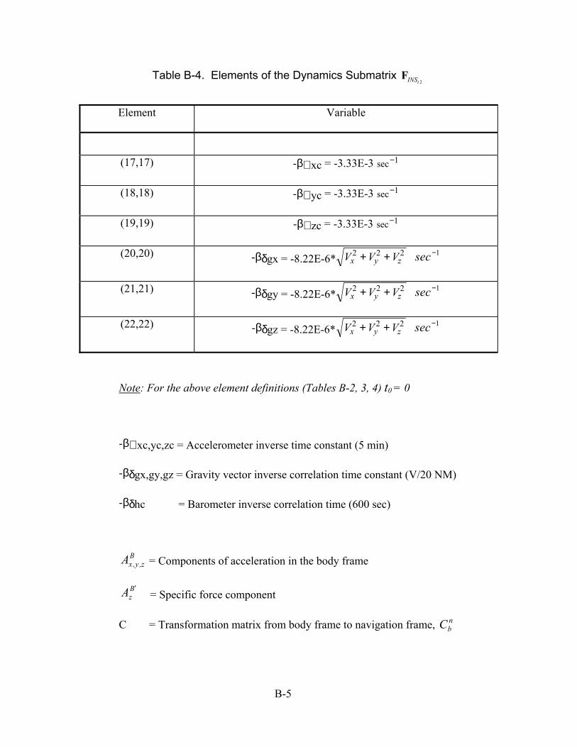
Table B-4. Elements of the Dynamics Submatrix 2tINSF
Element Variable
(17,17) -β∇ xc = -3.33E-3 sec −1
(18,18) -β∇ yc = -3.33E-3 sec −1
(19,19) -β∇ zc = -3.33E-3 sec −1
(20,20) -βδgx = -8.22E-6* V V Vx y z2 2 2+ + 1−sec
(21,21) -βδgy = -8.22E-6* V V Vx y z2 2 2+ + 1−sec
(22,22) -βδgz = -8.22E-6* V V Vx y z2 2 2+ + 1−sec
Note: For the above element definitions (Tables B-2, 3, 4) t0 = 0
-β∇ xc,yc,zc = Accelerometer inverse time constant (5 min)
-βδgx,gy,gz = Gravity vector inverse correlation time constant (V/20 NM)
-βδhc = Barometer inverse correlation time (600 sec)
Bz,y,xA = Components of acceleration in the body frame
BzA ′
= Specific force component
C = Transformation matrix from body frame to navigation frame, nbC
B- 5
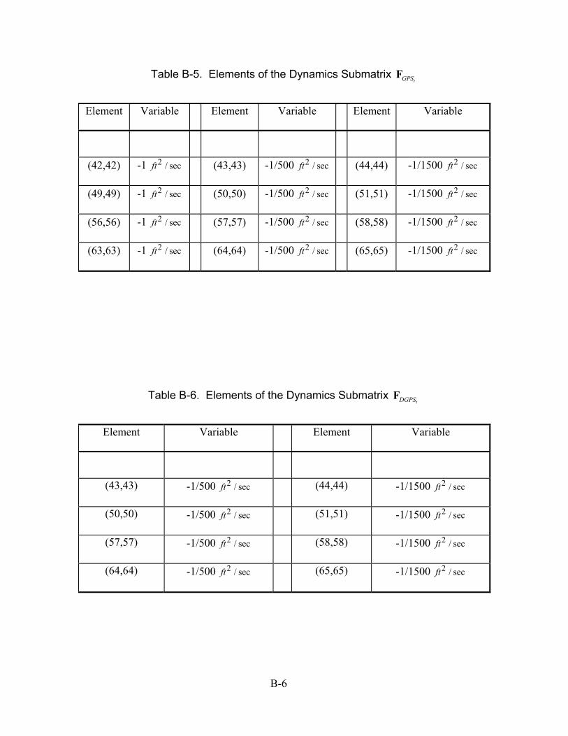
Table B-5. Elements of the Dynamics Submatrix tGPSF
Element Variable Element Variable Element Variable
(42,42) -1 ft2 / sec (43,43) -1/500 ft2 / sec (44,44) -1/1500 ft2 / sec
(49,49) -1 ft2 / sec (50,50) -1/500 ft2 / sec (51,51) -1/1500 ft2 / sec
(56,56) -1 ft2 / sec (57,57) -1/500 ft2 / sec (58,58) -1/1500 ft2 / sec
(63,63) -1 ft2 / sec (64,64) -1/500 ft2 / sec (65,65) -1/1500 ft2 / sec
Table B-6. Elements of the Dynamics Submatrix tDGPSF
Element Variable Element Variable
(43,43) -1/500 ft2 / sec (44,44) -1/1500 ft2 / sec
(50,50) -1/500 ft2 / sec (51,51) -1/1500 ft2 / sec
(57,57) -1/500 ft2 / sec (58,58) -1/1500 ft2 / sec
(64,64) -1/500 ft2 / sec (65,65) -1/1500 ft2 / sec
B- 6
B.2 Elements of the Process Noise and Measurement Noise Matrices
This section defines the dynamic noise strengths and measurement noise
variances for the truth and filter models. The truth model non-zero dynamics noise
strengths are defined in Tables B-7 through B-12. These noise strengths correspond to the
driving noises , , tINSw
tGPSwtDGPSw and in Equation (3.5). Note that the (4,4)
through (9,9) σ2 terms in Table B-7 are variable names as defined in the Litton technical
report [18] and do not represent variance terms typically associated with the notation σ2
[6,10]. They are actually the heights of Power Spectral Density (PSD) functions
associated with each white noise. However, the σ2
Filterw
terms in “2βi σi2 ” in (11,11) through
(24,24) are real variances (of the outputs of first order lag shaping filters). The filter
dynamics driving noise terms implemented after filter tuning for each respective INS
integration (0.4 nm/hr, 2.0 nm/hr and 4.0 nm/hr) is listed in Table B-10, Table B-11, and
Table B-12. Finally, the measurement noise variances used in the truth and filter models
are presented in Table B-13.
B- 7
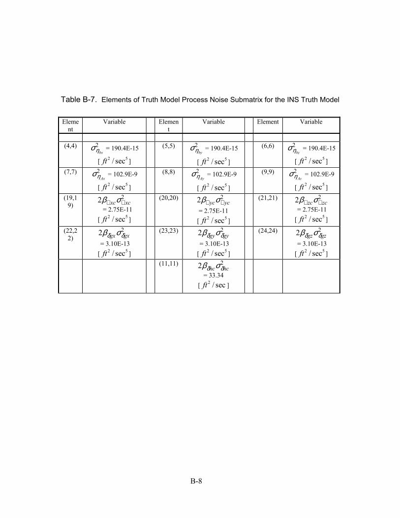
Table B-7. Elements of Truth Model Process Noise Submatrix for the INS Truth Model
Element
Variable Element
Variable Element Variable
(4,4) σηbx
2
ft
= 190.4E-15
[ ] 2 5/ sec
(5,5) σηby
2
ft
= 190.4E-15
[ ] 2 5/ sec
(6,6) σηbz
2
ft
= 190.4E-15
[ ] 2 5/ sec(7,7) σηAx
2
ft
= 102.9E-9
[ ] 2 5/ sec
(8,8) σηAy
2
ft
= 102.9E-9
[ ] 2 5/ sec
(9,9) σηAz
2
ft
= 102.9E-9
[ ] 2 5/ sec(19,1
9) 2 2β σ∇ ∇xc xc = 2.75E-11 [ ] 2 5/ secft
(20,20) 2 2β σ∇ ∇yc yc = 2.75E-11
[ ] 2 5/ secft
(21,21) 2 2β σ∇ ∇zc zc = 2.75E-11 [ ] 2 5/ secft
(22,22)
2 2β σδ δgx gx = 3.10E-13 [ ] 2 5/ secft
(23,23) 2 2β σδ δgy gy = 3.10E-13 [ ] 2 5/ secft
(24,24) 2 2β σδ δgz gz = 3.10E-13 [ ] 2 5/ secft
(11,11) 2 2β σδ δhc hc = 33.34
[ ] 2 / secft
B- 8
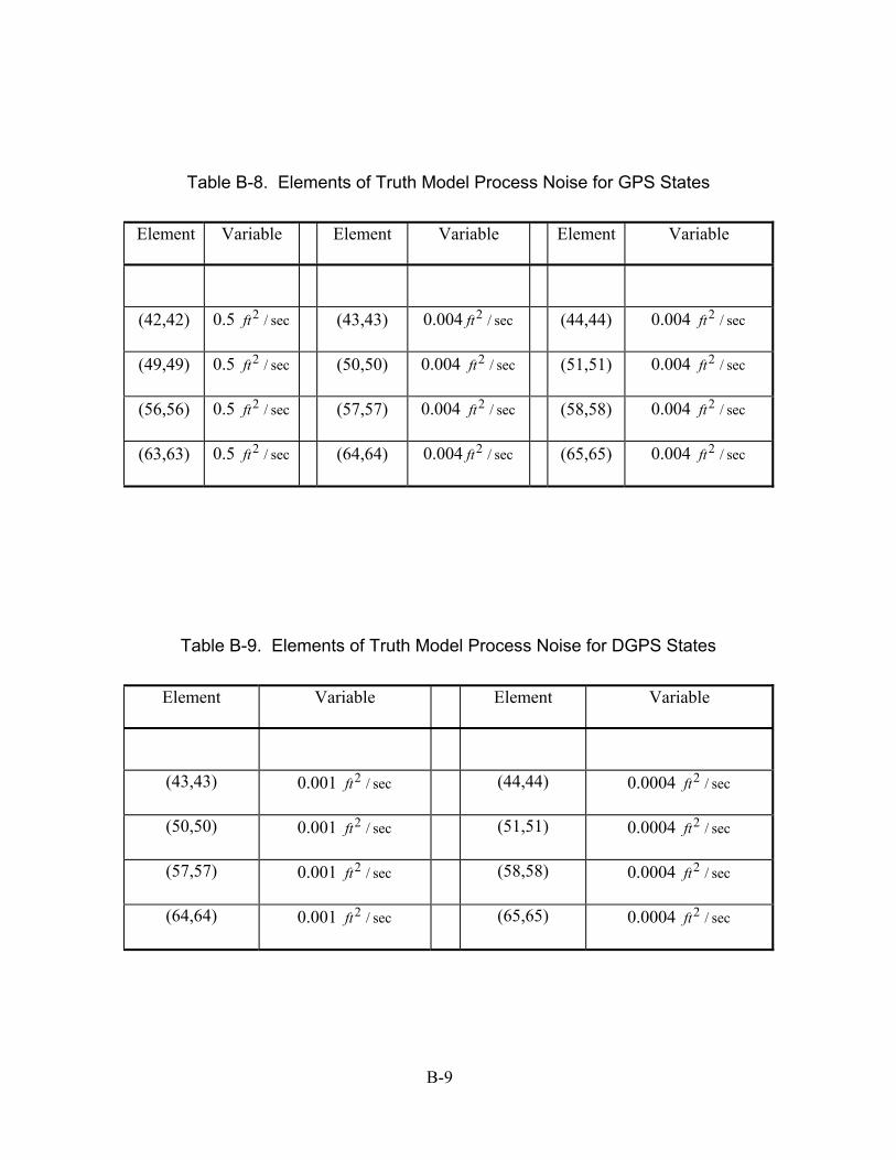
Table B-8. Elements of Truth Model Process Noise for GPS States
Element Variable Element Variable Element Variable
(42,42) 0.5 ft2 / sec (43,43) 0.004 ft2 / sec (44,44) 0.004 ft2 / sec
(49,49) 0.5 ft2 / sec (50,50) 0.004 ft2 / sec (51,51) 0.004 ft2 / sec
(56,56) 0.5 ft2 / sec (57,57) 0.004 ft2 / sec (58,58) 0.004 ft2 / sec
(63,63) 0.5 ft2 / sec (64,64) 0.004 ft2 / sec (65,65) 0.004 ft2 / sec
Table B-9. Elements of Truth Model Process Noise for DGPS States
Element Variable Element Variable
(43,43) 0.001 ft2 / sec (44,44) 0.0004 ft2 / sec
(50,50) 0.001 ft2 / sec (51,51) 0.0004 ft2 / sec
(57,57) 0.001 ft2 / sec (58,58) 0.0004 ft2 / sec
(64,64) 0.001 ft2 / sec (65,65) 0.0004 ft2 / sec
B- 9
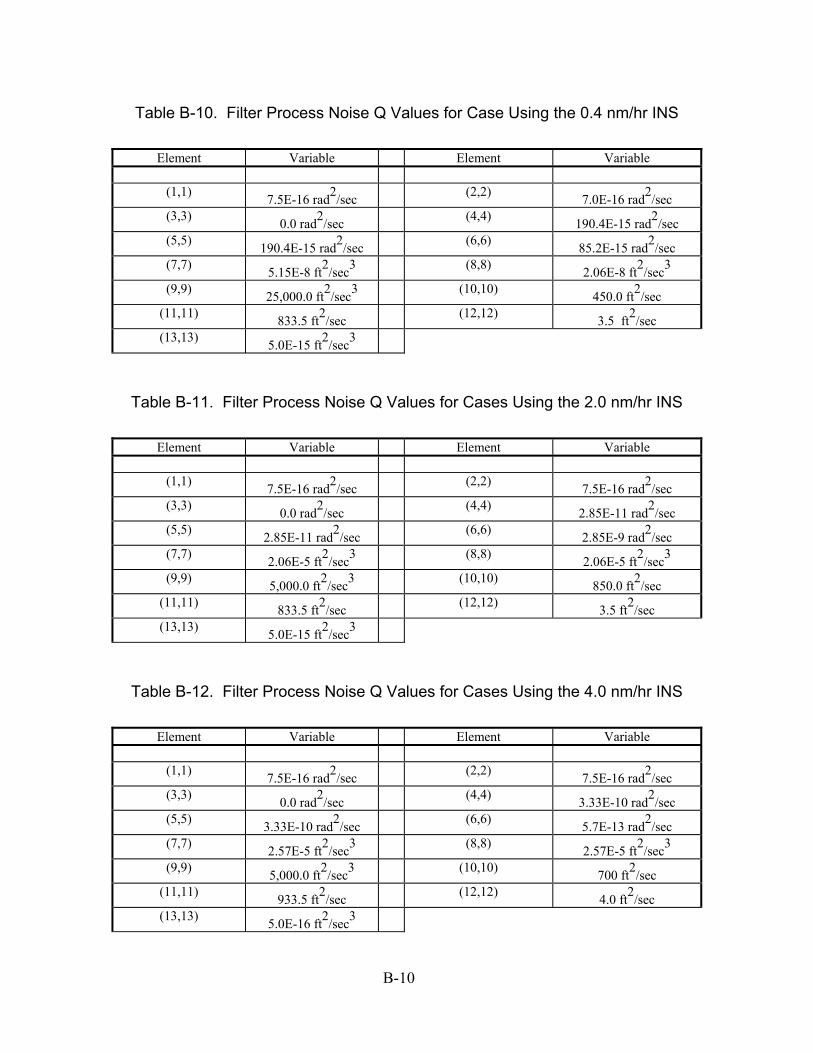
Table B-10. Filter Process Noise Q Values for Case Using the 0.4 nm/hr INS
Element Variable Element Variable
(1,1) 7.5E-16 rad2/sec (2,2) 7.0E-16 rad2/sec (3,3) 0.0 rad2/sec (4,4) 190.4E-15 rad2/sec (5,5) 190.4E-15 rad2/sec (6,6) 85.2E-15 rad2/sec (7,7) 5.15E-8 ft2/sec3 (8,8) 2.06E-8 ft2/sec3 (9,9) 25,000.0 ft2/sec3 (10,10) 450.0 ft2/sec
(11,11) 833.5 ft2/sec (12,12) 3.5 ft2/sec (13,13) 5.0E-15 ft2/sec3
Table B-11. Filter Process Noise Q Values for Cases Using the 2.0 nm/hr INS
Element Variable Element Variable
(1,1) 7.5E-16 rad2/sec (2,2) 7.5E-16 rad2/sec (3,3) 0.0 rad2/sec (4,4) 2.85E-11 rad2/sec (5,5) 2.85E-11 rad2/sec (6,6) 2.85E-9 rad2/sec (7,7) 2.06E-5 ft2/sec3 (8,8) 2.06E-5 ft2/sec3 (9,9) 5,000.0 ft2/sec3 (10,10) 850.0 ft2/sec
(11,11) 833.5 ft2/sec (12,12) 3.5 ft2/sec (13,13) 5.0E-15 ft2/sec3
Table B-12. Filter Process Noise Q Values for Cases Using the 4.0 nm/hr INS
Element Variable Element Variable
(1,1) 7.5E-16 rad2/sec (2,2) 7.5E-16 rad2/sec (3,3) 0.0 rad2/sec (4,4) 3.33E-10 rad2/sec (5,5) 3.33E-10 rad2/sec (6,6) 5.7E-13 rad2/sec (7,7) 2.57E-5 ft2/sec3 (8,8) 2.57E-5 ft2/sec3 (9,9) 5,000.0 ft2/sec3 (10,10) 700 ft2/sec
(11,11) 933.5 ft2/sec (12,12) 4.0 ft2/sec (13,13) 5.0E-16 ft2/sec3
B- 10
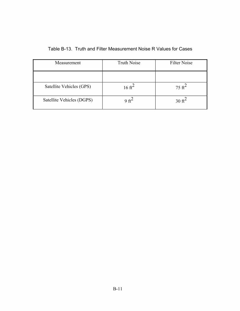
Table B-13. Truth and Filter Measurement Noise R Values for Cases
Measurement Truth Noise Filter Noise
Satellite Vehicles (GPS) 16 ft2 75 ft2
Satellite Vehicles (DGPS) 9 ft2 30 ft2
B- 11
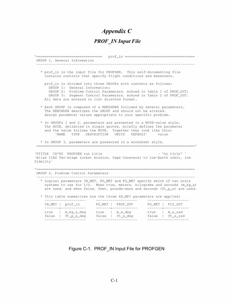
Appendix C PROF_IN Input File
"================================ prof_in ==================================GROUP 1, General Information-----------------------------------------------------------------------------
* prof_in is the input file for PROFGEN. This self-documenting filecontains controls that specify flight conditions and maneuvers.
prof_in is divided into three GROUPs with contents as follows:GROUP 1: General Information;GROUP 2: Problem Control Parameters, echoed in Table 1 of PROF_OUT;GROUP 3: Segment Control Parameters, echoed in Table 2 of PROF_OUT.
All data are entered in list directed format.
* Each GROUP is composed of a REMINDER followed by several parameters.The REMINDER describes the GROUP and should not be altered.Assign parameter values appropriate to your specific problem.
* In GROUPs 1 and 2, parameters are presented in a NOTE-value style.The NOTE, delimited in single quotes, briefly defines the parameterand the value follows the NOTE. Together they look like this:
'NAME TYPE DESCRIPTION UNITS DEFAULT' value
* In GROUP 3, parameters are presented in a worksheet style.============================================================================="
'PTITLE CH*80 PROFGEN run title - "no title" ''Atlas IIAS Two-stage rocket mission, Cape Canaveral to low-Earth orbit, lowfidelity'
"=============================================================================GROUP 2, Problem Control Parameters-----------------------------------------------------------------------------
* Logical parameters IN_MET, PO_MET and FO_MET specify which of two unitssystems to use for I/O. When true, meters, kilograms and seconds (m_kg_s)are used, and when false, feet, pounds-mass and seconds (ft_p_s) are used.
* This table summarizes how the three XX_MET parameters are applied:-------------------- -------------------- --------------------IN_MET | prof_in PO_MET | PROF_OUT FO_MET | FLY_OUT-------+------------ -------+------------ -------+------------true | m_kg_s_deg true | m_s_deg true | m_s_radfalse | ft_p_s_deg false | ft_s_deg false | ft_s_rad-------------------- -------------------- --------------------
Figure C-1. PROF_IN Input File for PROFGEN
C- 1
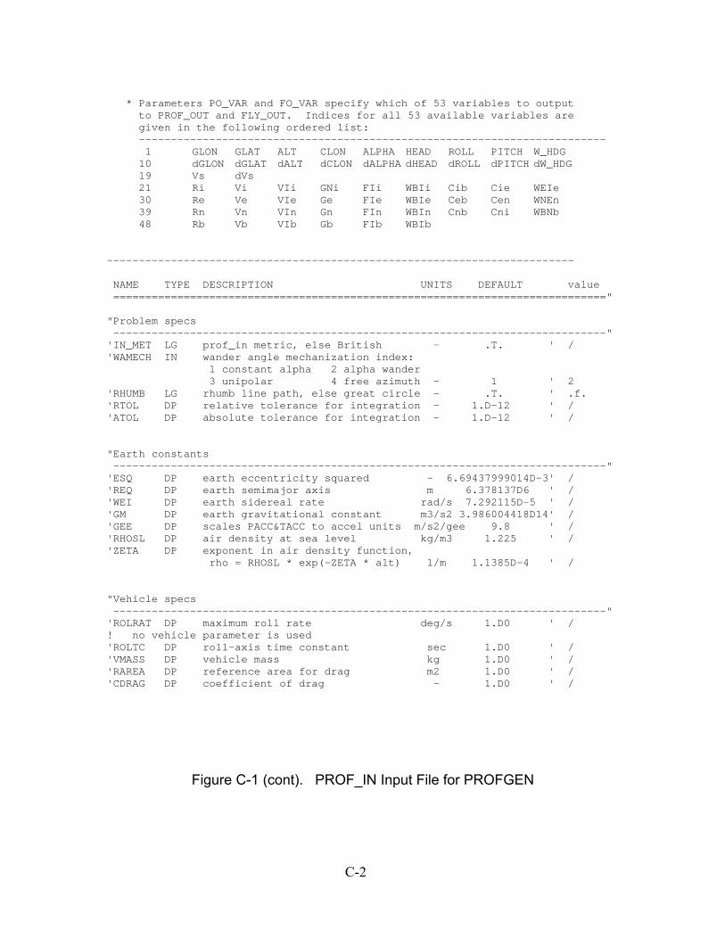
* Parameters PO_VAR and FO_VAR specify which of 53 variables to outputto PROF_OUT and FLY_OUT. Indices for all 53 available variables aregiven in the following ordered list:-------------------------------------------------------------------------1 GLON GLAT ALT CLON ALPHA HEAD ROLL PITCH W_HDG10 dGLON dGLAT dALT dCLON dALPHA dHEAD dROLL dPITCH dW_HDG19 Vs dVs21 Ri Vi VIi GNi FIi WBIi Cib Cie WEIe30 Re Ve VIe Ge FIe WBIe Ceb Cen WNEn39 Rn Vn VIn Gn FIn WBIn Cnb Cni WBNb48 Rb Vb VIb Gb FIb WBIb
-------------------------------------------------------------------------
NAME TYPE DESCRIPTION UNITS DEFAULT value============================================================================="
"Problem specs-----------------------------------------------------------------------------"
'IN_MET LG prof_in metric, else British - .T. ' /'WAMECH IN wander angle mechanization index:
1 constant alpha 2 alpha wander3 unipolar 4 free azimuth - 1 ' 2
'RHUMB LG rhumb line path, else great circle - .T. ' .f.'RTOL DP relative tolerance for integration - 1.D-12 ' /'ATOL DP absolute tolerance for integration - 1.D-12 ' /
"Earth constants-----------------------------------------------------------------------------"
'ESQ DP earth eccentricity squared - 6.69437999014D-3' /'REQ DP earth semimajor axis m 6.378137D6 ' /'WEI DP earth sidereal rate rad/s 7.292115D-5 ' /'GM DP earth gravitational constant m3/s2 3.986004418D14' /'GEE DP scales PACC&TACC to accel units m/s2/gee 9.8 ' /'RHOSL DP air density at sea level kg/m3 1.225 ' /'ZETA DP exponent in air density function,
rho = RHOSL * exp(-ZETA * alt) 1/m 1.1385D-4 ' /
"Vehicle specs-----------------------------------------------------------------------------"
'ROLRAT DP maximum roll rate deg/s 1.D0 ' /! no vehicle parameter is used'ROLTC DP roll-axis time constant sec 1.D0 ' /'VMASS DP vehicle mass kg 1.D0 ' /'RAREA DP reference area for drag m2 1.D0 ' /'CDRAG DP coefficient of drag - 1.D0 ' /
Figure C-1 (cont). PROF_IN Input File for PROFGEN
C- 2
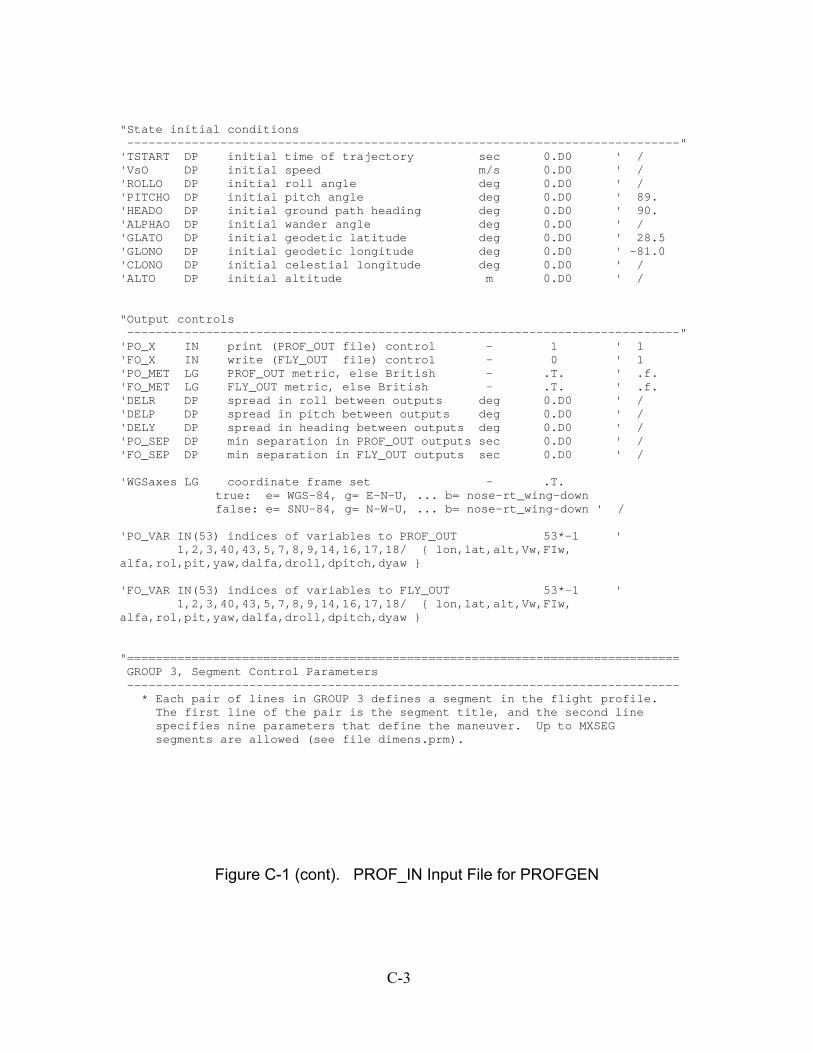
"State initial conditions-----------------------------------------------------------------------------"
'TSTART DP initial time of trajectory sec 0.D0 ' /'VsO DP initial speed m/s 0.D0 ' /'ROLLO DP initial roll angle deg 0.D0 ' /'PITCHO DP initial pitch angle deg 0.D0 ' 89.'HEADO DP initial ground path heading deg 0.D0 ' 90.'ALPHAO DP initial wander angle deg 0.D0 ' /'GLATO DP initial geodetic latitude deg 0.D0 ' 28.5'GLONO DP initial geodetic longitude deg 0.D0 ' -81.0'CLONO DP initial celestial longitude deg 0.D0 ' /'ALTO DP initial altitude m 0.D0 ' /
"Output controls-----------------------------------------------------------------------------"
'PO_X IN print (PROF_OUT file) control - 1 ' 1'FO_X IN write (FLY_OUT file) control - 0 ' 1'PO_MET LG PROF_OUT metric, else British - .T. ' .f.'FO_MET LG FLY_OUT metric, else British - .T. ' .f.'DELR DP spread in roll between outputs deg 0.D0 ' /'DELP DP spread in pitch between outputs deg 0.D0 ' /'DELY DP spread in heading between outputs deg 0.D0 ' /'PO_SEP DP min separation in PROF_OUT outputs sec 0.D0 ' /'FO_SEP DP min separation in FLY_OUT outputs sec 0.D0 ' /
'WGSaxes LG coordinate frame set - .T.true: e= WGS-84, g= E-N-U, ... b= nose-rt_wing-downfalse: e= SNU-84, g= N-W-U, ... b= nose-rt_wing-down ' /
'PO_VAR IN(53) indices of variables to PROF_OUT 53*-1 '1,2,3,40,43,5,7,8,9,14,16,17,18/ lon,lat,alt,Vw,FIw,
alfa,rol,pit,yaw,dalfa,droll,dpitch,dyaw
'FO_VAR IN(53) indices of variables to FLY_OUT 53*-1 '1,2,3,40,43,5,7,8,9,14,16,17,18/ lon,lat,alt,Vw,FIw,
alfa,rol,pit,yaw,dalfa,droll,dpitch,dyaw
"=============================================================================GROUP 3, Segment Control Parameters-----------------------------------------------------------------------------
* Each pair of lines in GROUP 3 defines a segment in the flight profile.The first line of the pair is the segment title, and the second linespecifies nine parameters that define the maneuver. Up to MXSEGsegments are allowed (see file dimens.prm).
Figure C-1 (cont). PROF_IN Input File for PROFGEN
C- 3
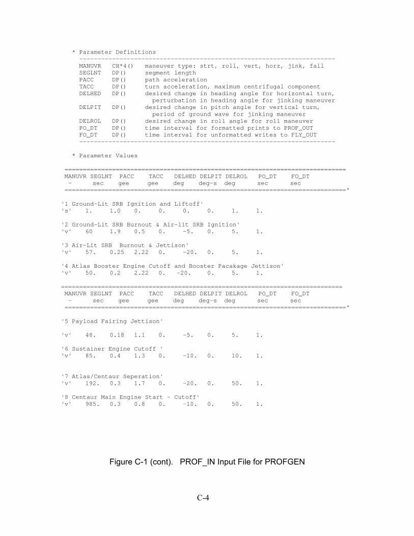
* Parameter Definitions----------------------------------------------------------------------MANUVR CH*4() maneuver type: strt, roll, vert, horz, jink, fallSEGLNT DP() segment lengthPACC DP() path accelerationTACC DP() turn acceleration, maximum centrifugal componentDELHED DP() desired change in heading angle for horizontal turn,
perturbation in heading angle for jinking maneuverDELPIT DP() desired change in pitch angle for vertical turn,
period of ground wave for jinking maneuverDELROL DP() desired change in roll angle for roll maneuverPO_DT DP() time interval for formatted prints to PROF_OUTFO_DT DP() time interval for unformatted writes to FLY_OUT----------------------------------------------------------------------
* Parameter Values
=============================================================================MANUVR SEGLNT PACC TACC DELHED DELPIT DELROL PO_DT FO_DT- sec gee gee deg deg-s deg sec sec
============================================================================="
'1 Ground-Lit SRB Ignition and Liftoff''s' 1. 1.0 0. 0. 0. 0. 1. 1.
'2 Ground-Lit SRB Burnout & Air-lit SRB Ignition''v' 60 1.9 0.5 0. -5. 0. 5. 1.
'3 Air-Lit SRB Burnout & Jettison''v' 57. 0.25 2.22 0. -20. 0. 5. 1.
'4 Atlas Booster Engine Cutoff and Booster Pacakage Jettison''v' 50. 0.2 2.22 0. -20. 0. 5. 1.
=============================================================================MANUVR SEGLNT PACC TACC DELHED DELPIT DELROL PO_DT FO_DT- sec gee gee deg deg-s deg sec sec
============================================================================="
'5 Payload Fairing Jettison'
'v' 48. 0.18 1.1 0. -5. 0. 5. 1.
'6 Sustainer Engine Cutoff ''v' 85. 0.4 1.3 0. -10. 0. 10. 1.
'7 Atlas/Centaur Seperation''v' 192. 0.3 1.7 0. -20. 0. 50. 1.
'8 Centaur Main Engine Start - Cutoff''v' 985. 0.3 0.8 0. -10. 0. 50. 1.
Figure C-1 (cont). PROF_IN Input File for PROFGEN
C- 4
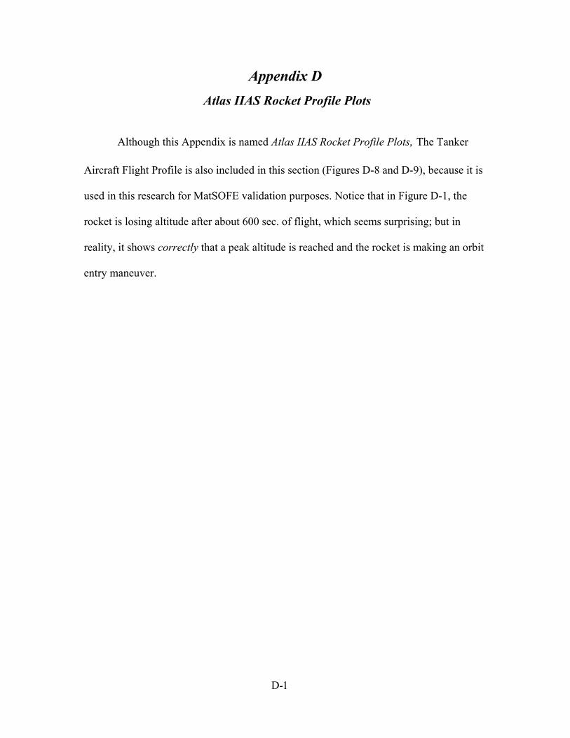
Appendix D Atlas IIAS Rocket Profile Plots
Although this Appendix is named Atlas IIAS Rocket Profile Plots, The Tanker
Aircraft Flight Profile is also included in this section (Figures D-8 and D-9), because it is
used in this research for MatSOFE validation purposes. Notice that in Figure D-1, the
rocket is losing altitude after about 600 sec. of flight, which seems surprising; but in
reality, it shows correctly that a peak altitude is reached and the rocket is making an orbit
entry maneuver.
D- 1
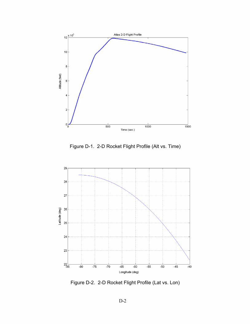
Figure D-1. 2-D Rocket Flight Profile (Alt vs. Time)
Figure D-2. 2-D Rocket Flight Profile (Lat vs. Lon)
D- 2
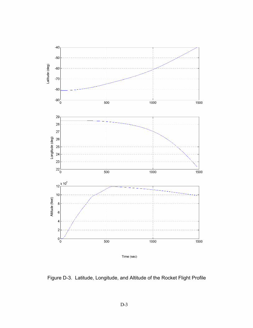
Figure D-3. Latitude, Longitude, and Altitude of the Rocket Flight Profile
D- 3
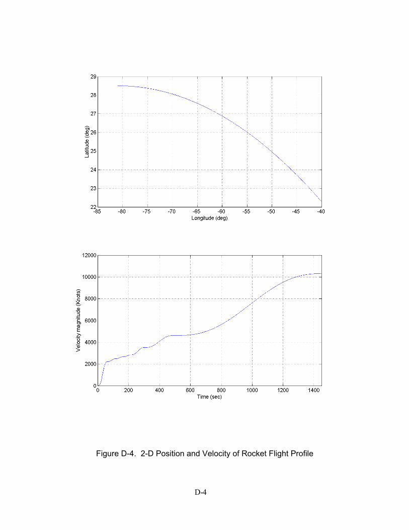
Figure D-4. 2-D Position and Velocity of Rocket Flight Profile
D- 4
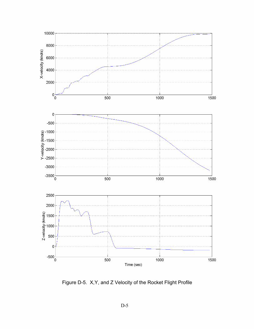
Figure D-5. X,Y, and Z Velocity of the Rocket Flight Profile
D- 5
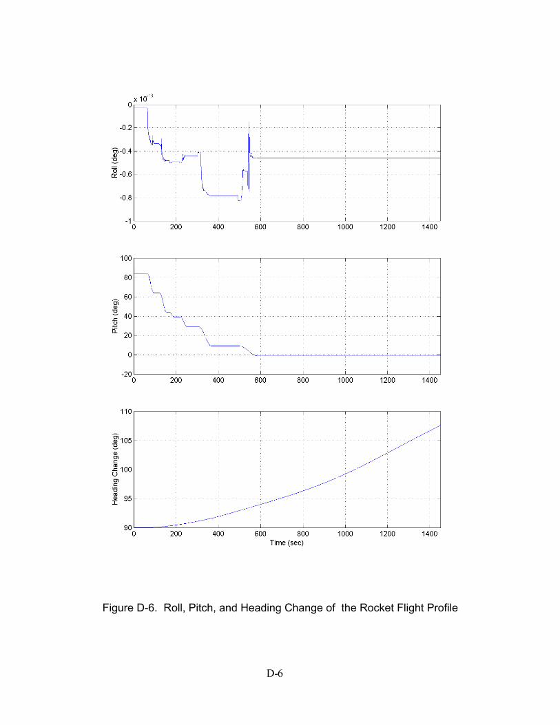
Figure D-6. Roll, Pitch, and Heading Change of the Rocket Flight Profile
D- 6
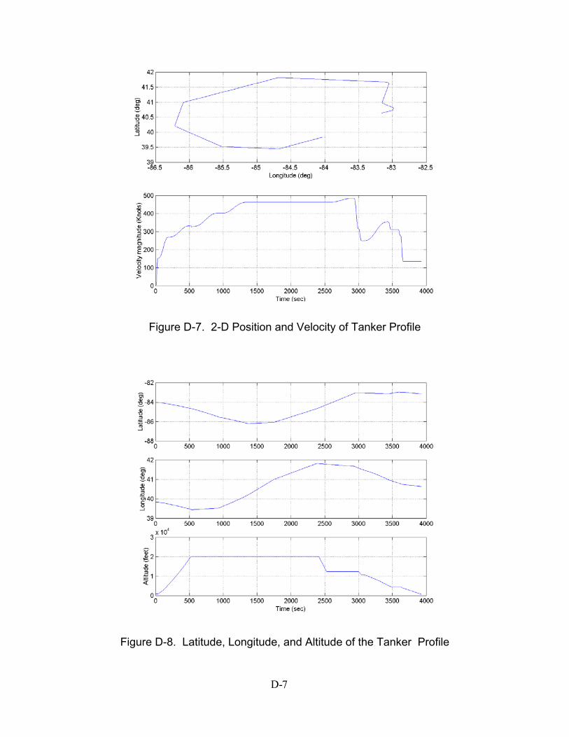
Figure D-7. 2-D Position and Velocity of Tanker Profile
Figure D-8. Latitude, Longitude, and Altitude of the Tanker Profile
D- 7
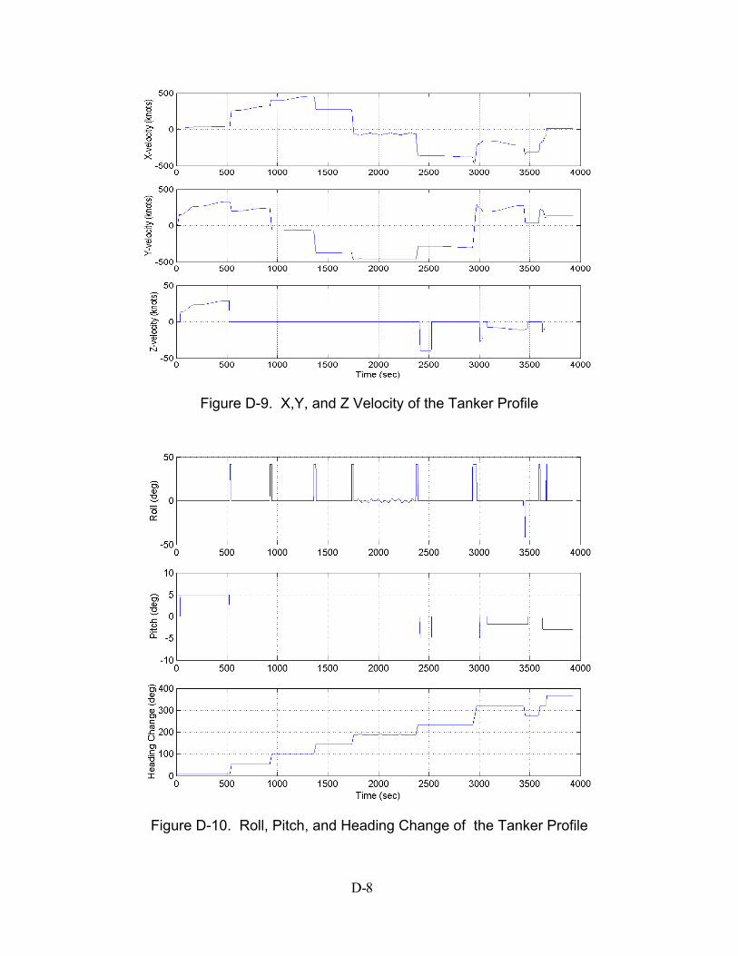
Figure D-9. X,Y, and Z Velocity of the Tanker Profile
Figure D-10. Roll, Pitch, and Heading Change of the Tanker Profile
D- 8

Appendix E True Ephemeris Generation Process
E- 1
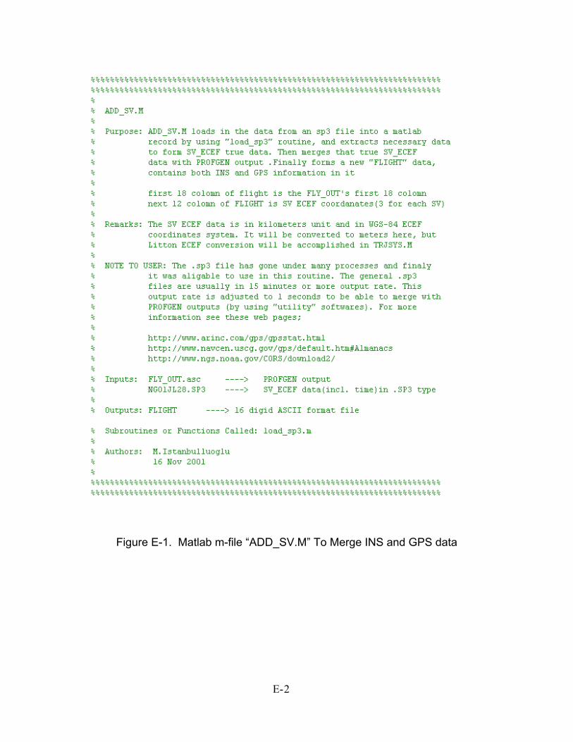
Figure E-1. Matlab m-file “ADD_SV.M” To Merge INS and GPS data
E- 2
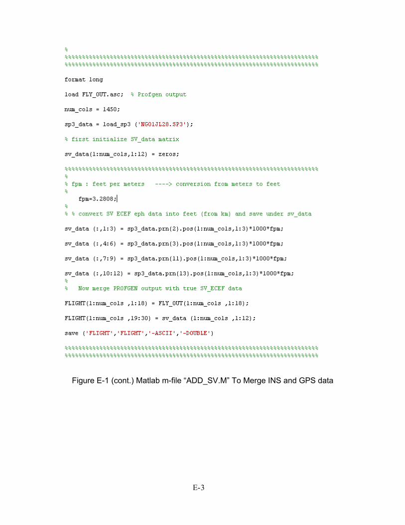
Figure E-1 (cont.) Matlab m-file “ADD_SV.M” To Merge INS and GPS data
E- 3
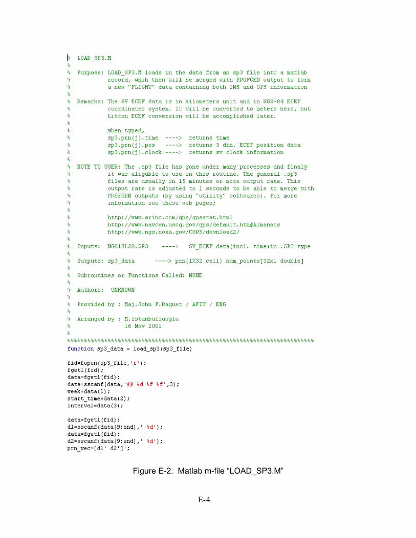
Figure E-2. Matlab m-file “LOAD_SP3.M”
E- 4
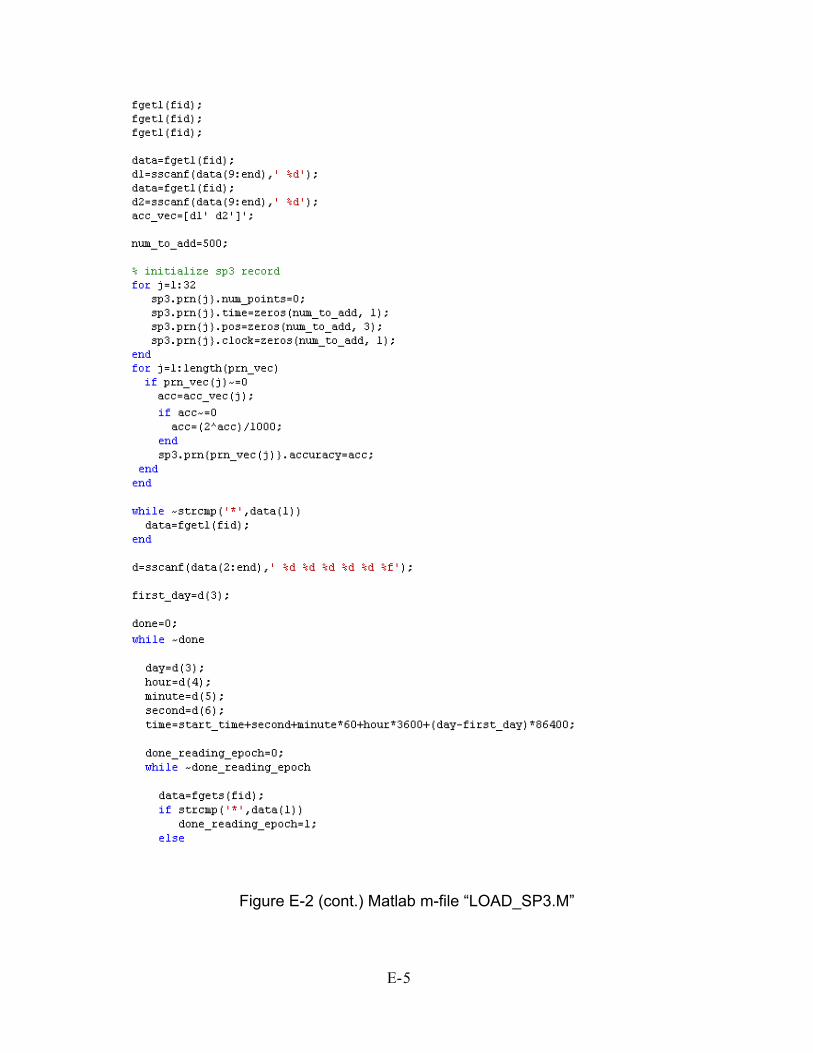
Figure E-2 (cont.) Matlab m-file “LOAD_SP3.M”
E- 5
Figure E-2 (cont.) Matlab m-file “LOAD_SP3.M”
E- 6
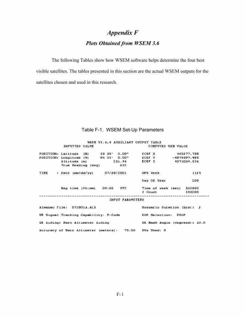
Appendix F Plots Obtained from WSEM 3.6
The following Tables show how WSEM software helps determine the four best
visible satellites. The tables presented in this section are the actual WSEM outputs for the
satellites chosen and used in this research.
Table F-1. WSEM Set-Up Parameters
F- 1
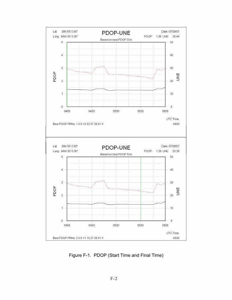
Figure F-1. PDOP (Start Time and Final Time)
F- 2
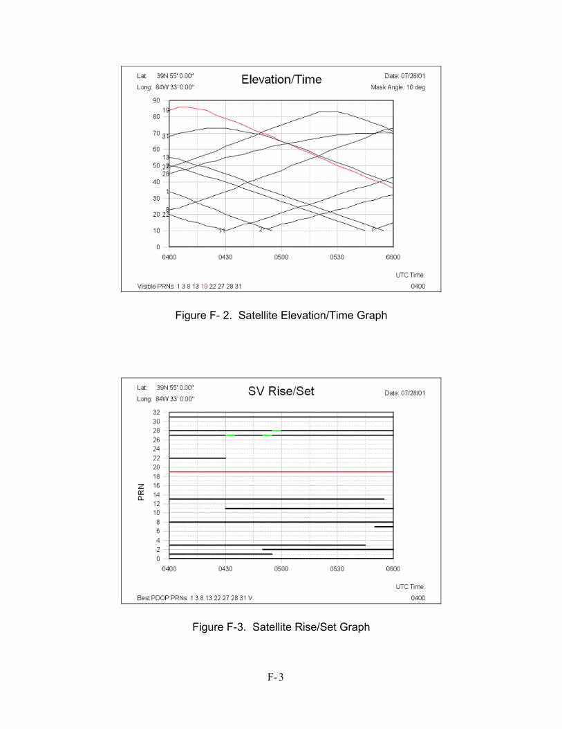
Figure F- 2. Satellite Elevation/Time Graph
Figure F-3. Satellite Rise/Set Graph
F- 3
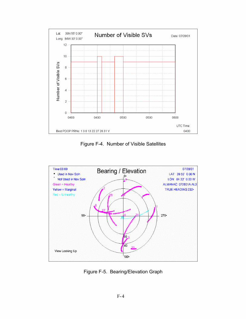
Figure F-4. Number of Visible Satellites
Figure F-5. Bearing/Elevation Graph
F- 4
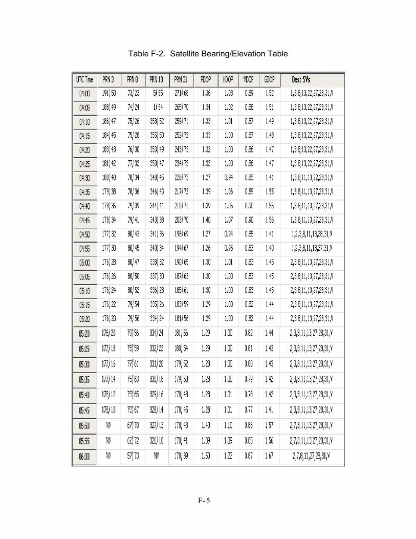
Table F-2. Satellite Bearing/Elevation Table
F- 5

Appendix G MatSOFE Validation Plots
G- 1
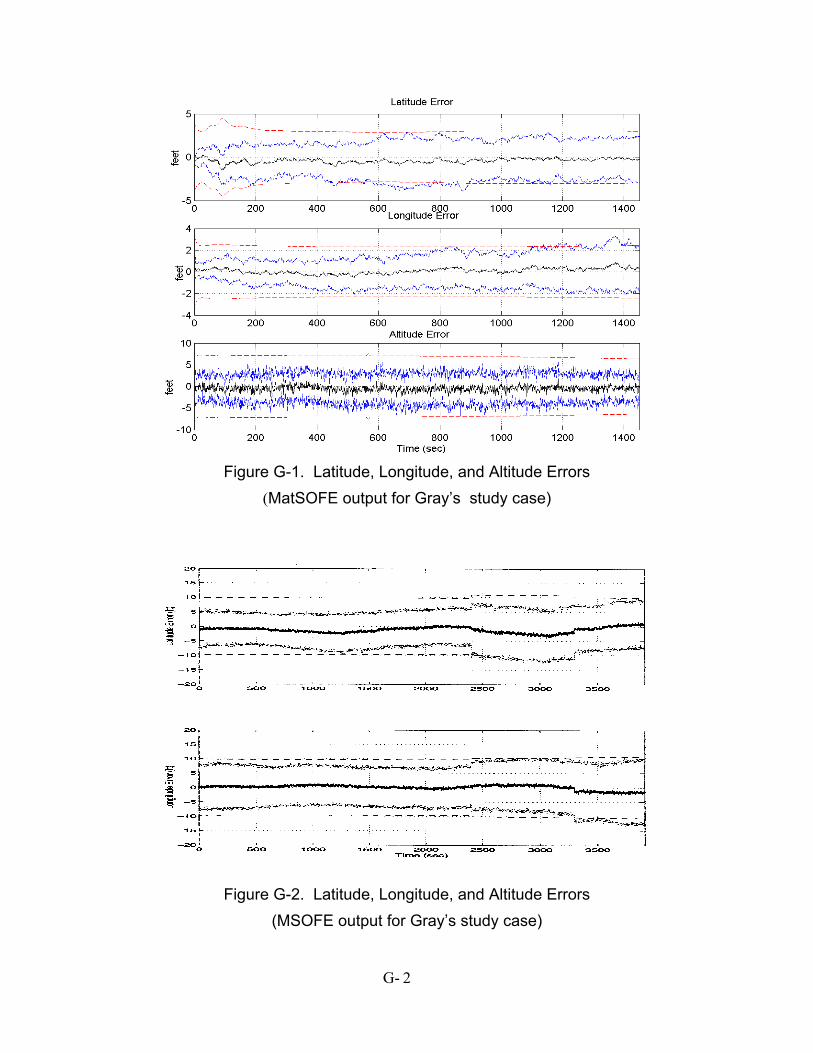
Figure G-1. Latitude, Longitude, and Altitude Errors
(MatSOFE output for Gray’s study case)
Figure G-2. Latitude, Longitude, and Altitude Errors (MSOFE output for Gray’s study case)
G- 2
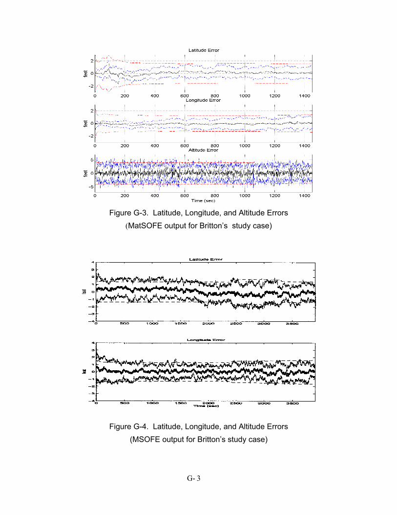
Figure G-3. Latitude, Longitude, and Altitude Errors
(MatSOFE output for Britton’s study case)
Figure G-4. Latitude, Longitude, and Altitude Errors (MSOFE output for Britton’s study case)
G- 3
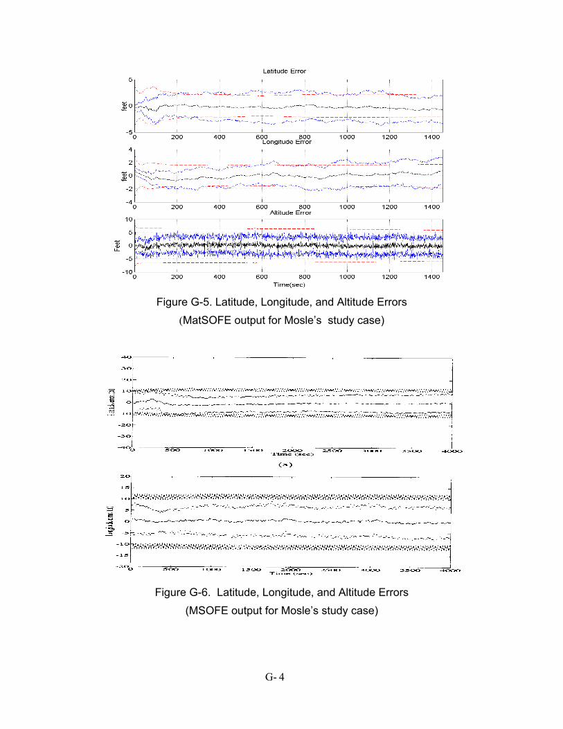
Figure G-5. Latitude, Longitude, and Altitude Errors
(MatSOFE output for Mosle’s study case)
Figure G-6. Latitude, Longitude, and Altitude Errors
(MSOFE output for Mosle’s study case)
G- 4

Appendix H Tuning Examples
Plot legend:sample mean error
…… true error (sample mean error )
------ filter-predicted error (0 )
trueσ±
filterσ±
H- 1
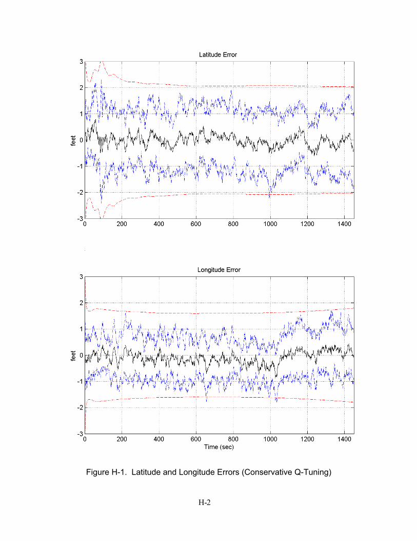
Figure H-1. Latitude and Longitude Errors (Conservative Q-Tuning)
H- 2
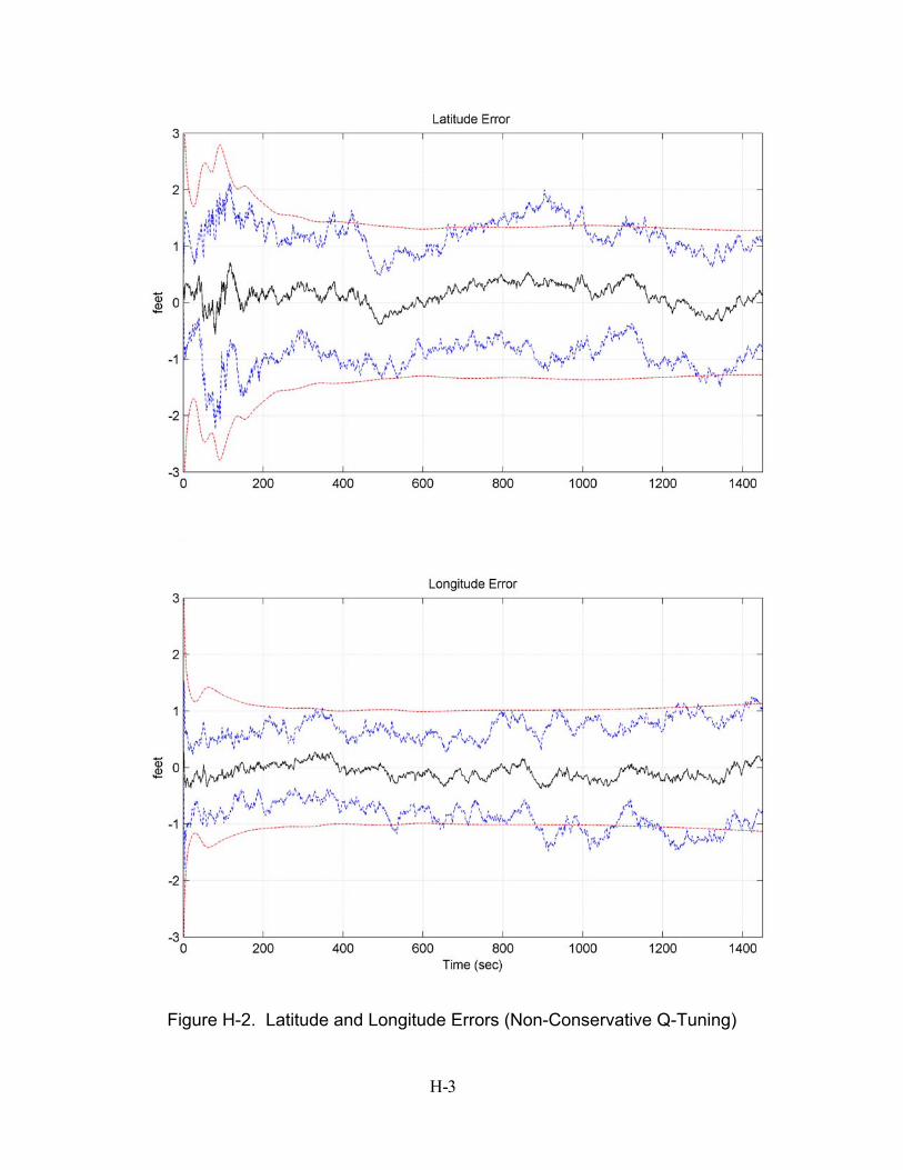
Figure H-2. Latitude and Longitude Errors (Non-Conservative Q-Tuning)
H- 3
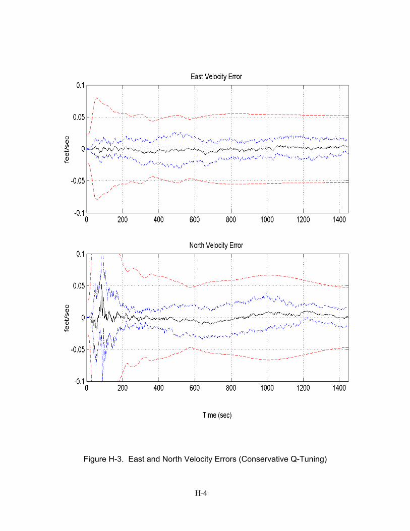
Figure H-3. East and North Velocity Errors (Conservative Q-Tuning)
H- 4
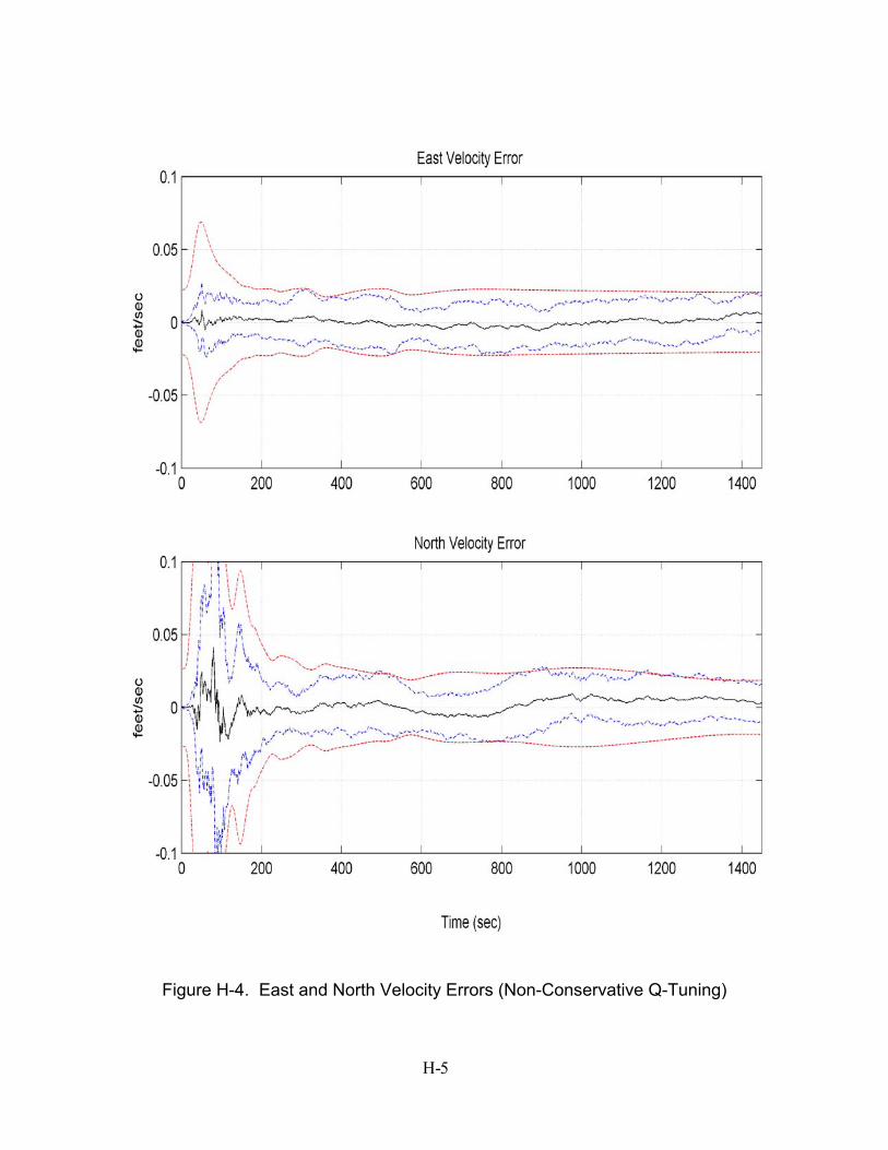
Figure H-4. East and North Velocity Errors (Non-Conservative Q-Tuning)
H- 5
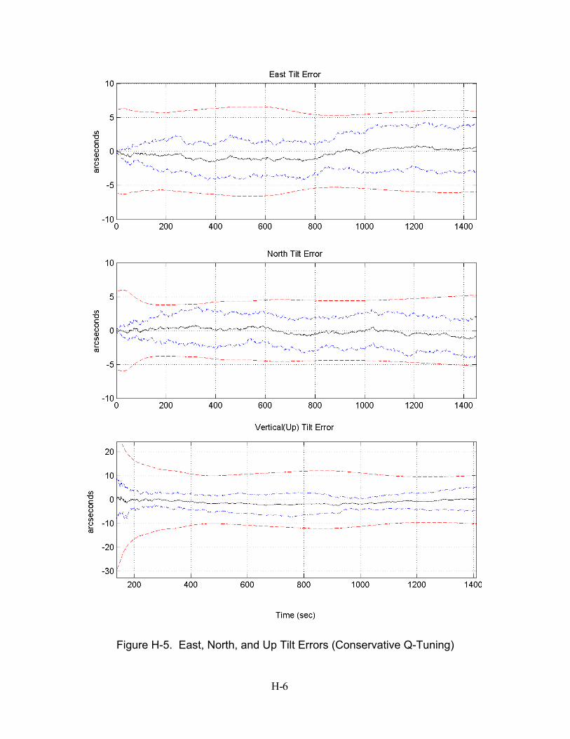
Figure H-5. East, North, and Up Tilt Errors (Conservative Q-Tuning)
H- 6
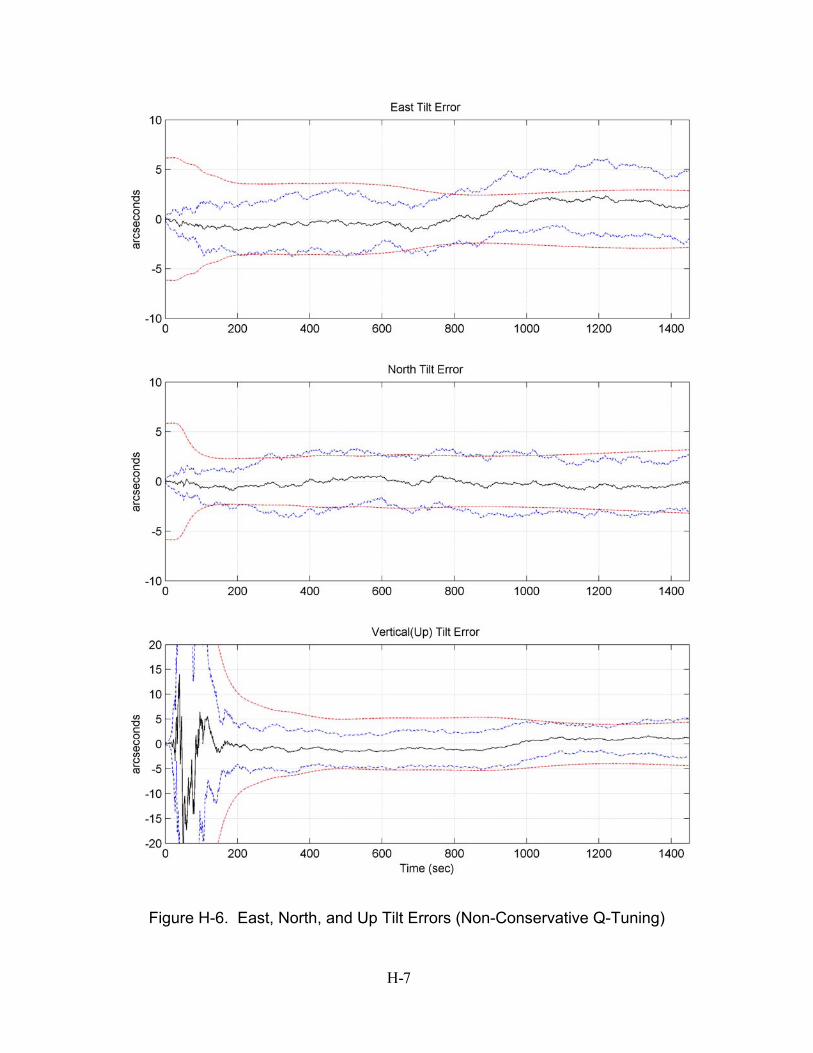
Figure H-6. East, North, and Up Tilt Errors (Non-Conservative Q-Tuning)
H- 7
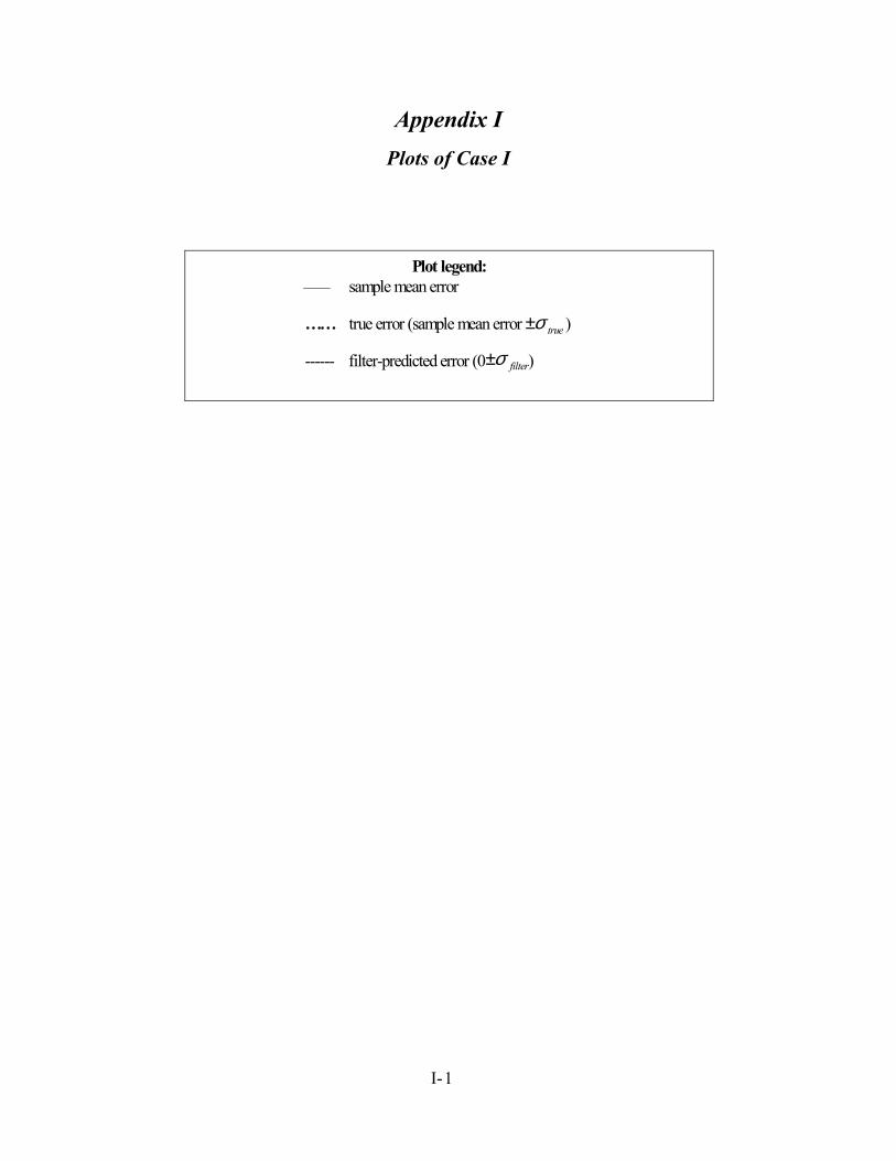
Appendix I Plots of Case I
Plot legend:sample mean error
…… true error (sample mean error )
------ filter-predicted error (0 )
trueσ±
filterσ±
I- 1
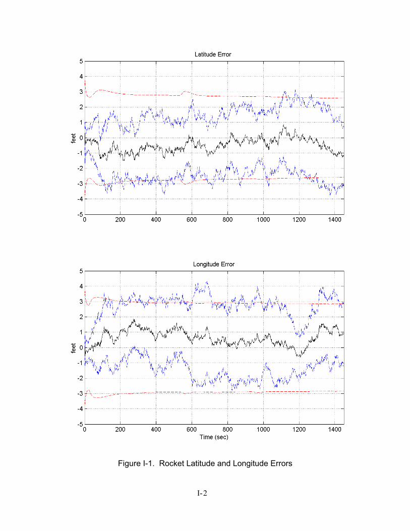
Figure I-1. Rocket Latitude and Longitude Errors
I- 2
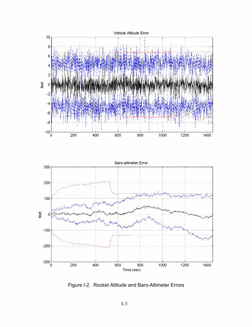
Figure I-2. Rocket Altitude and Baro-Altimeter Errors
I- 3
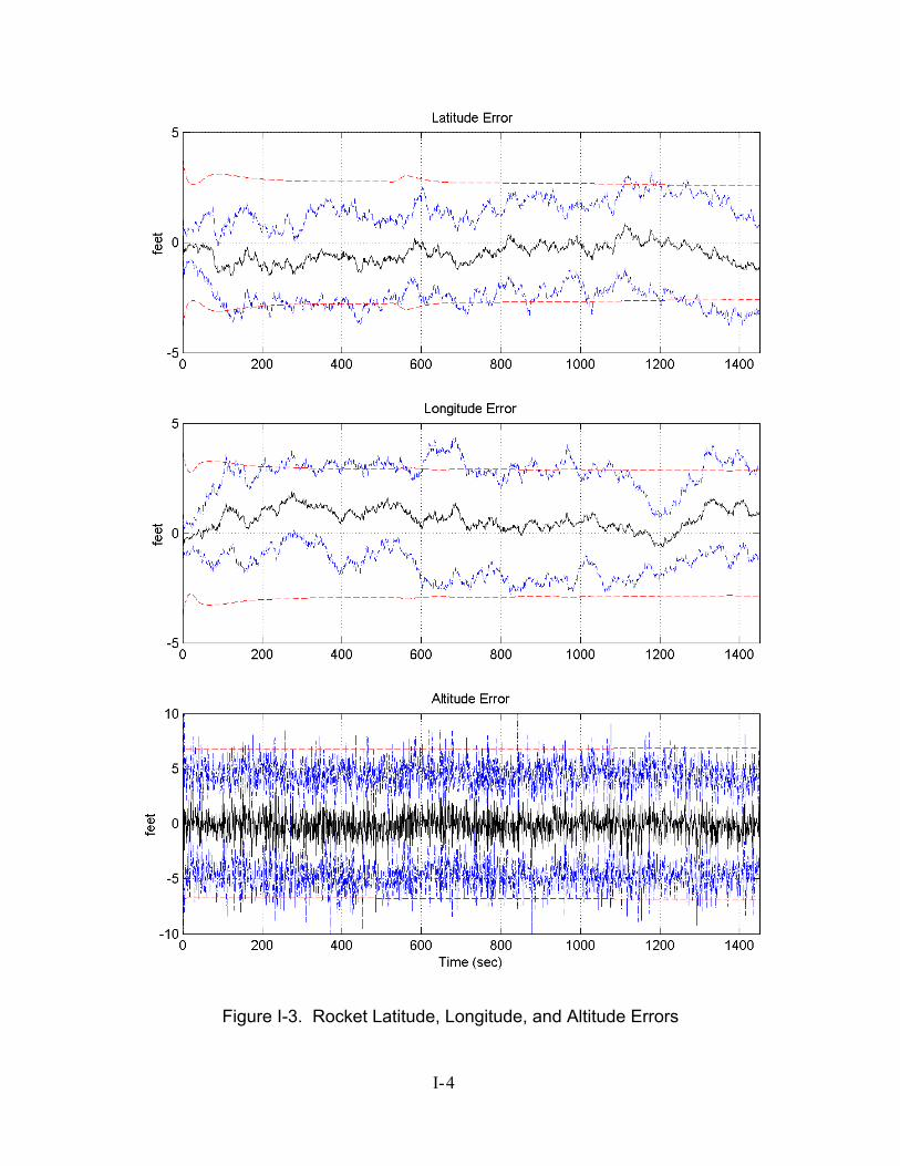
Figure I-3. Rocket Latitude, Longitude, and Altitude Errors
I- 4
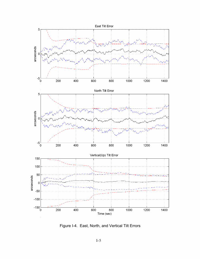
Figure I-4. East, North, and Vertical Tilt Errors
I- 5
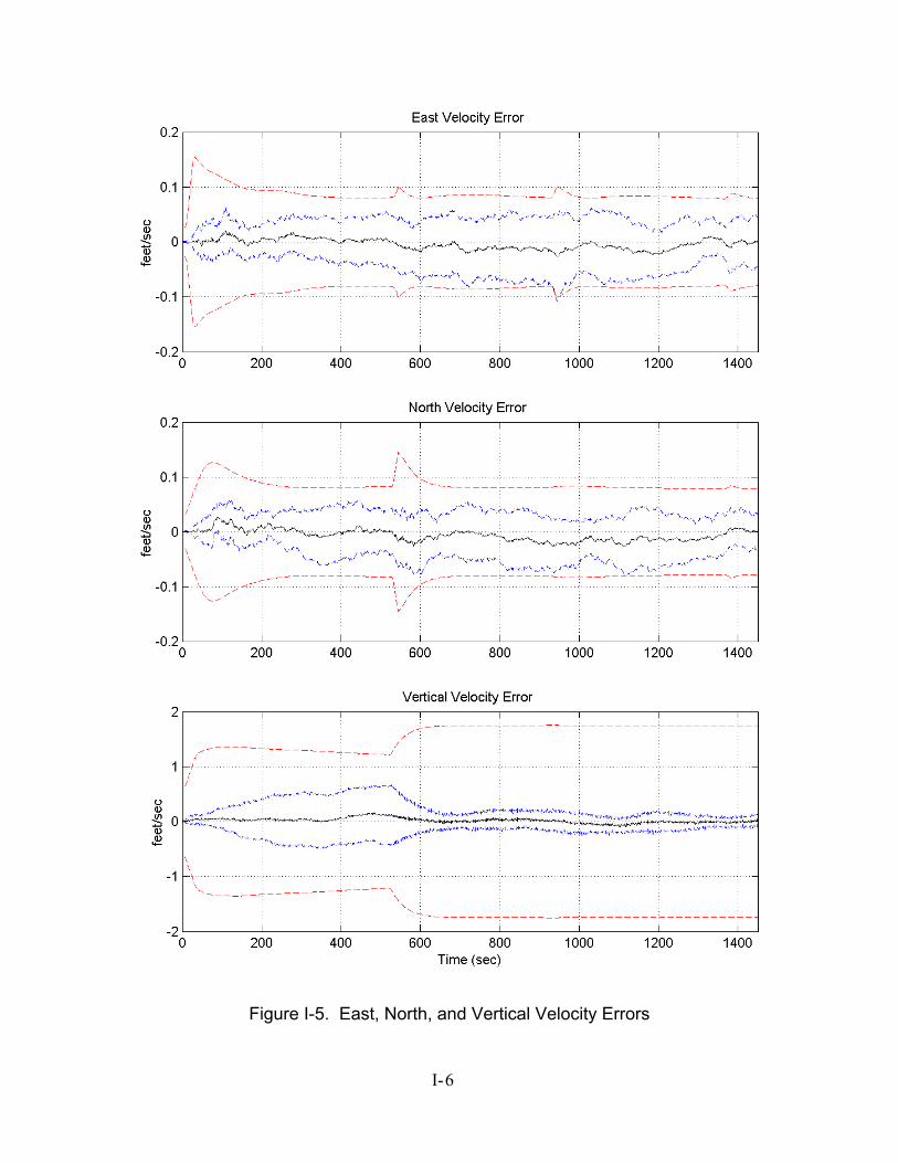
Figure I-5. East, North, and Vertical Velocity Errors
I- 6
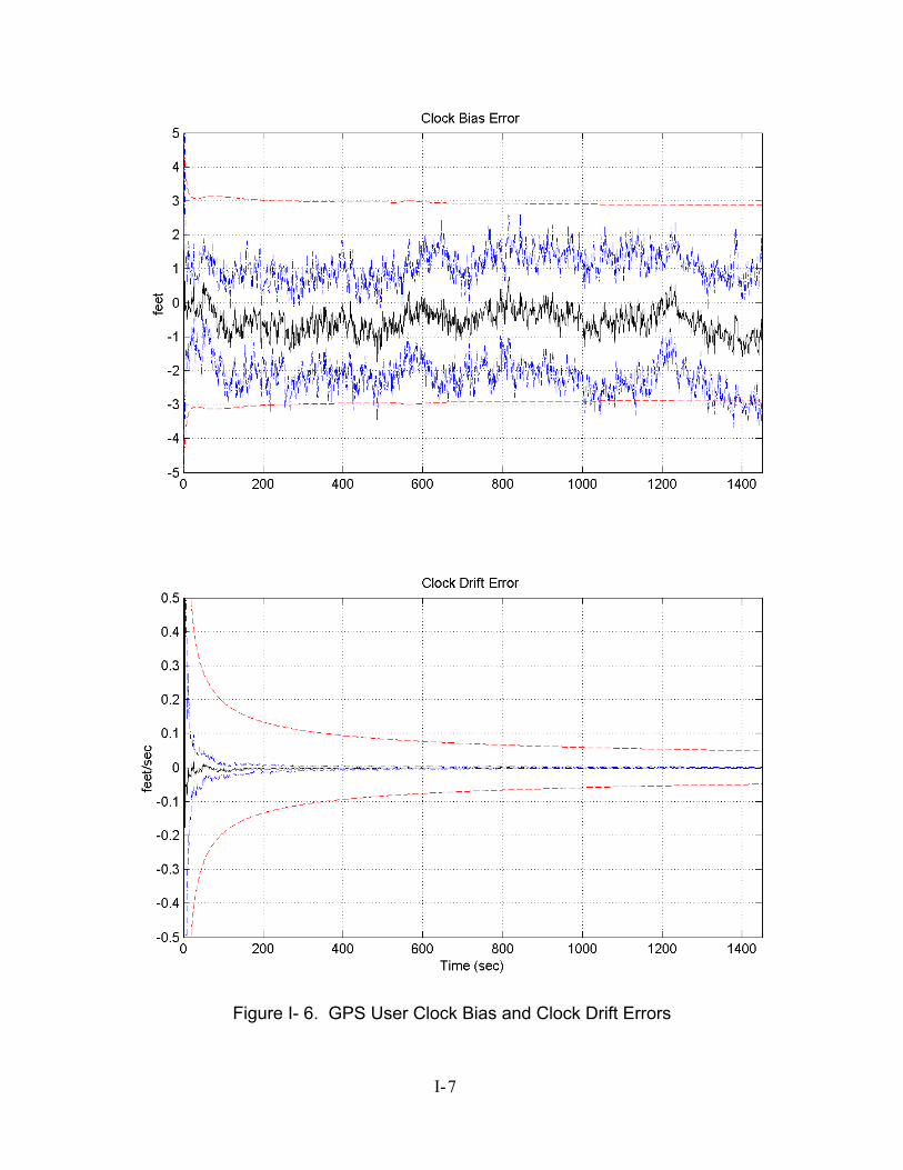
Figure I- 6. GPS User Clock Bias and Clock Drift Errors
I- 7
Appendix J Plots of Case II
Plot legend:sample mean error
…… true error (sample mean error )
------ filter-predicted error (0 )
trueσ±
filterσ±
J- 1
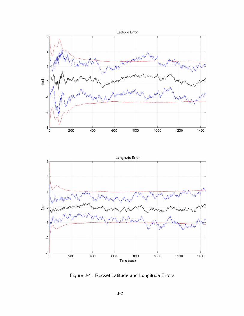
Figure J-1. Rocket Latitude and Longitude Errors
J- 2
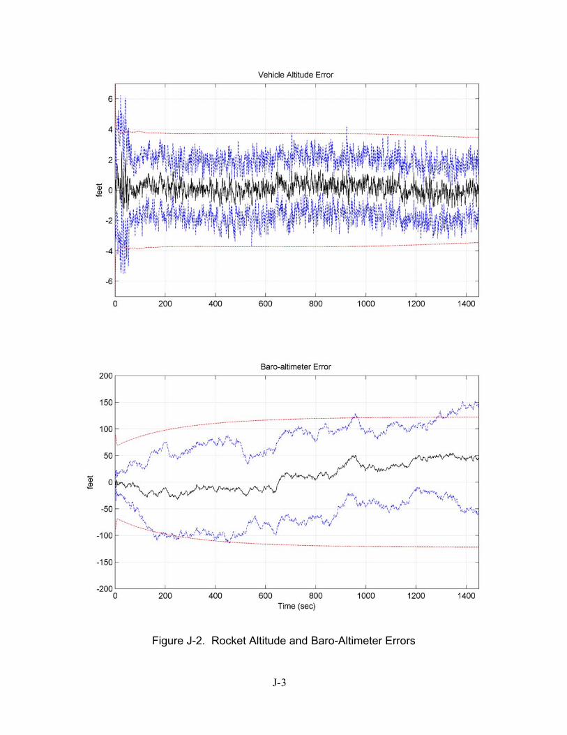
Figure J-2. Rocket Altitude and Baro-Altimeter Errors
J- 3
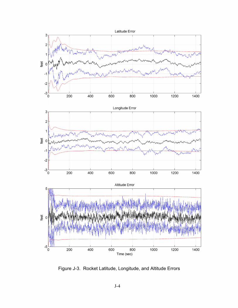
Figure J-3. Rocket Latitude, Longitude, and Altitude Errors
J- 4
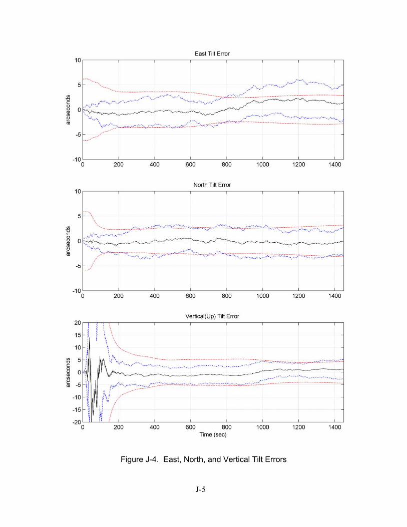
Figure J-4. East, North, and Vertical Tilt Errors
J- 5
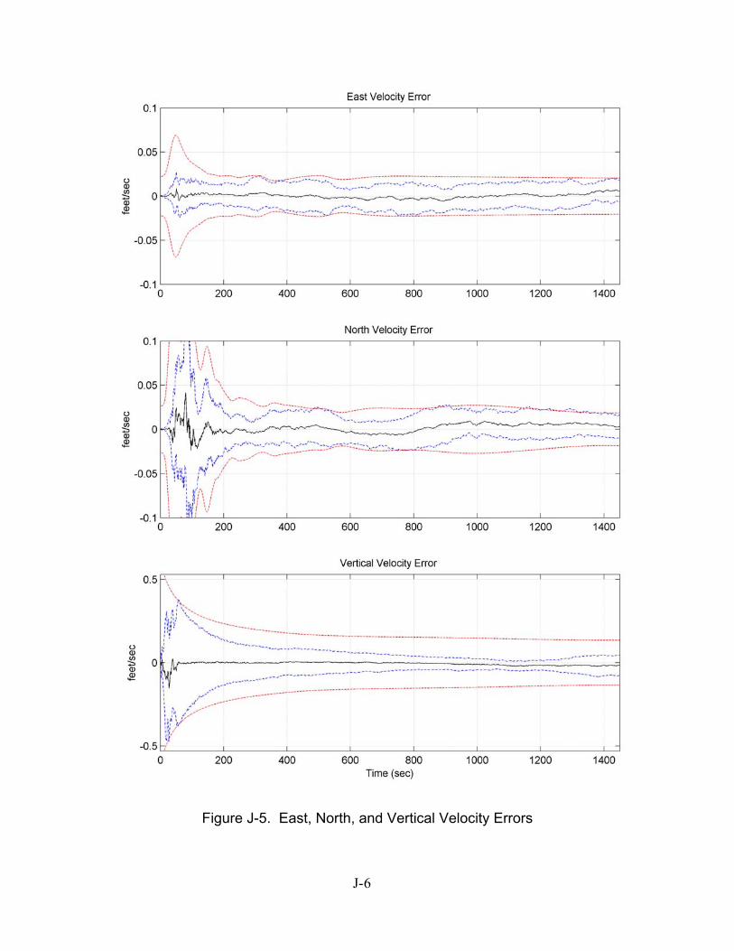
Figure J-5. East, North, and Vertical Velocity Errors
J- 6
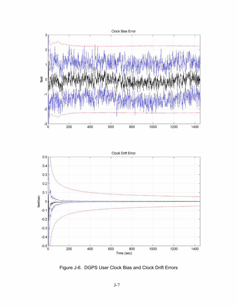
Figure J-6. DGPS User Clock Bias and Clock Drift Errors
J- 7

Appendix K Plots of Case III
Plot legend:sample mean error
…… true error (sample mean error )
------ filter-predicted error (0 )
trueσ±
filterσ±
K- 1
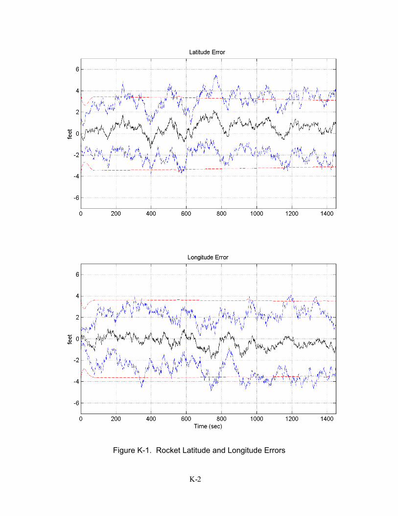
Figure K-1. Rocket Latitude and Longitude Errors
K- 2
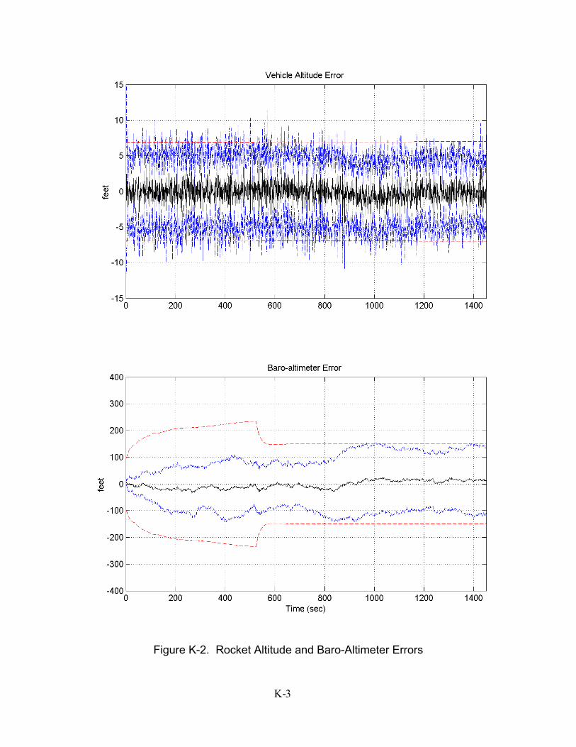
Figure K-2. Rocket Altitude and Baro-Altimeter Errors
K- 3
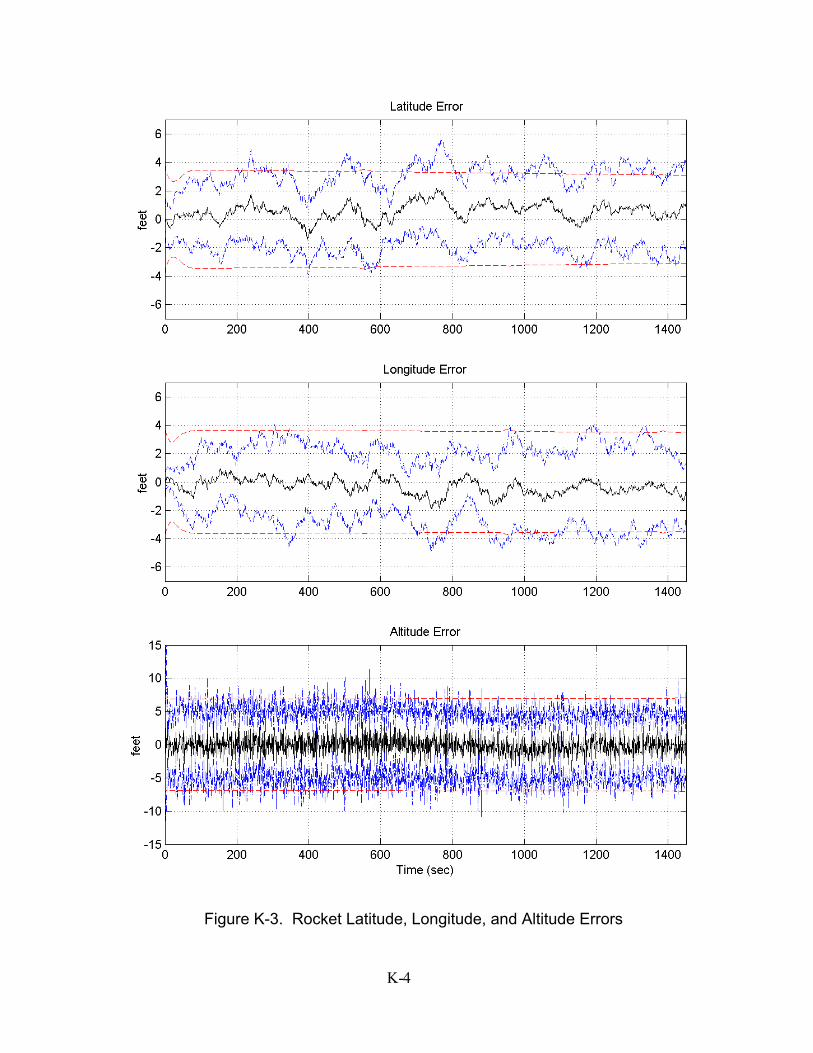
Figure K-3. Rocket Latitude, Longitude, and Altitude Errors
K- 4
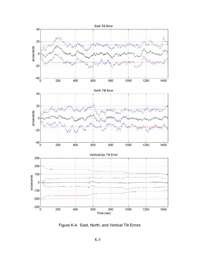
Figure K-4. East, North, and Vertical Tilt Errors
K- 5
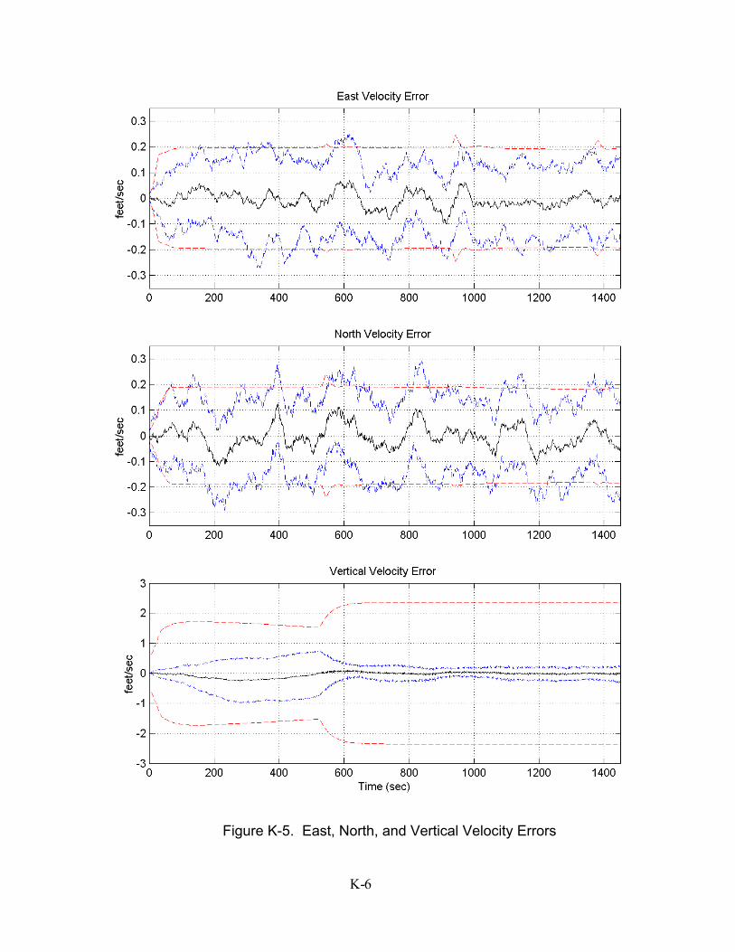
Figure K-5. East, North, and Vertical Velocity Errors
K- 6
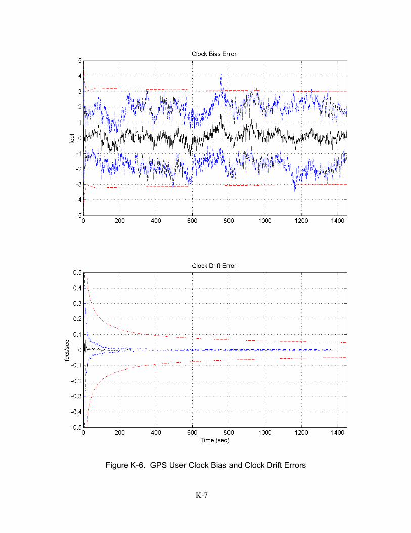
Figure K-6. GPS User Clock Bias and Clock Drift Errors
K- 7

Appendix L Plots of Case IV
Plot legend:sample mean error
…… true error (sample mean error )
------ filter-predicted error (0 )
trueσ±
filterσ±
L- 1
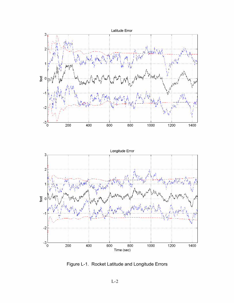
Figure L-1. Rocket Latitude and Longitude Errors
L- 2
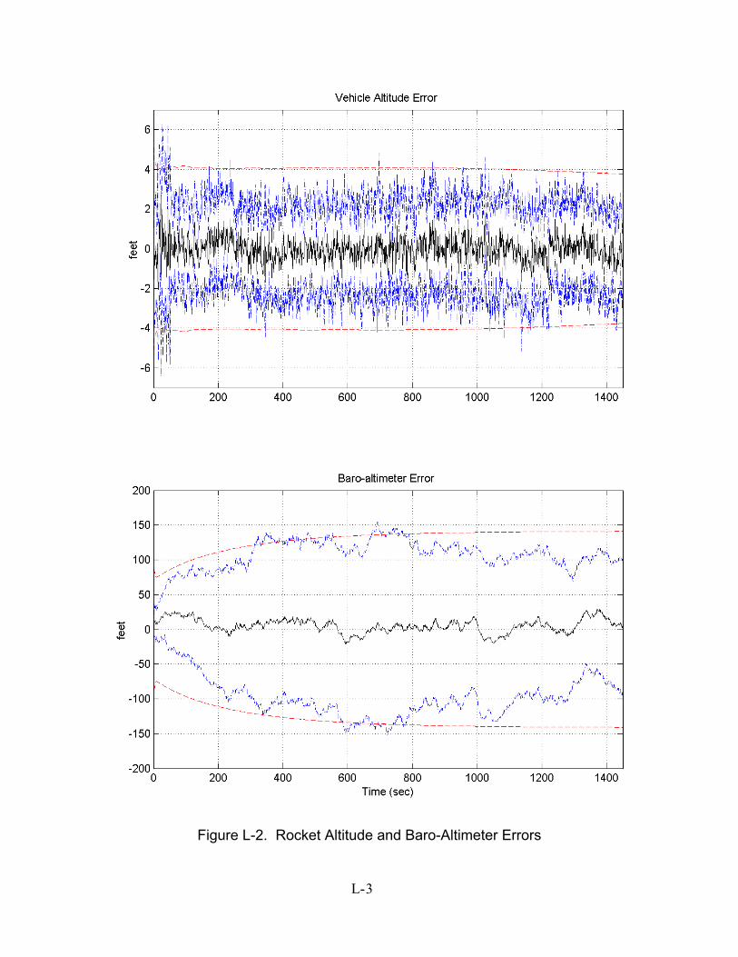
Figure L-2. Rocket Altitude and Baro-Altimeter Errors
L- 3
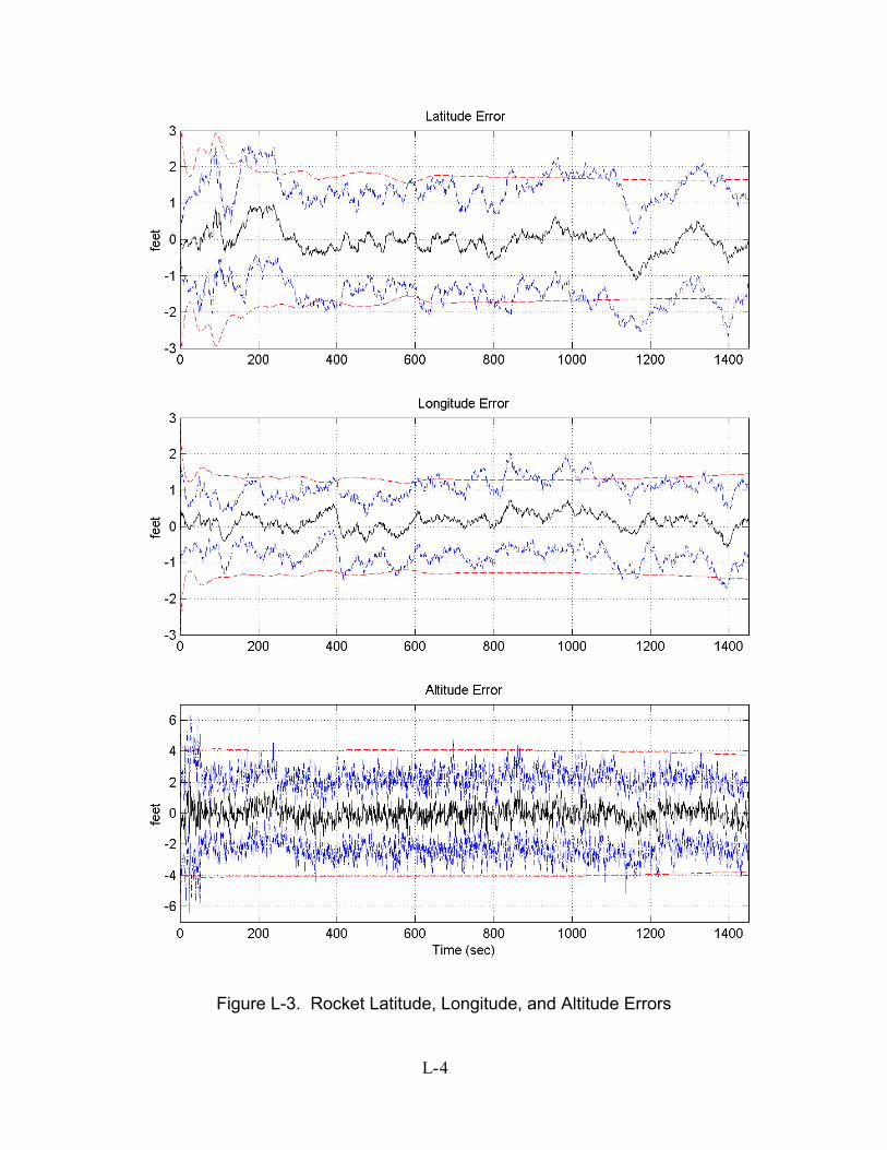
Figure L-3. Rocket Latitude, Longitude, and Altitude Errors
L- 4
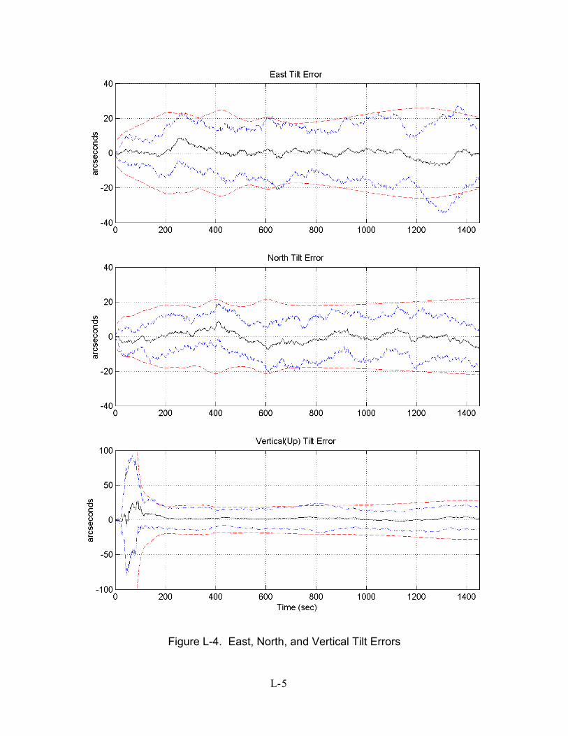
Figure L-4. East, North, and Vertical Tilt Errors
L- 5
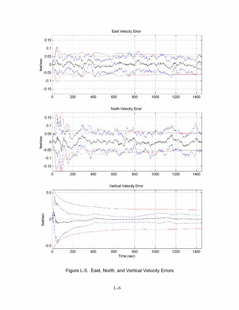
Figure L-5. East, North, and Vertical Velocity Errors
L- 6
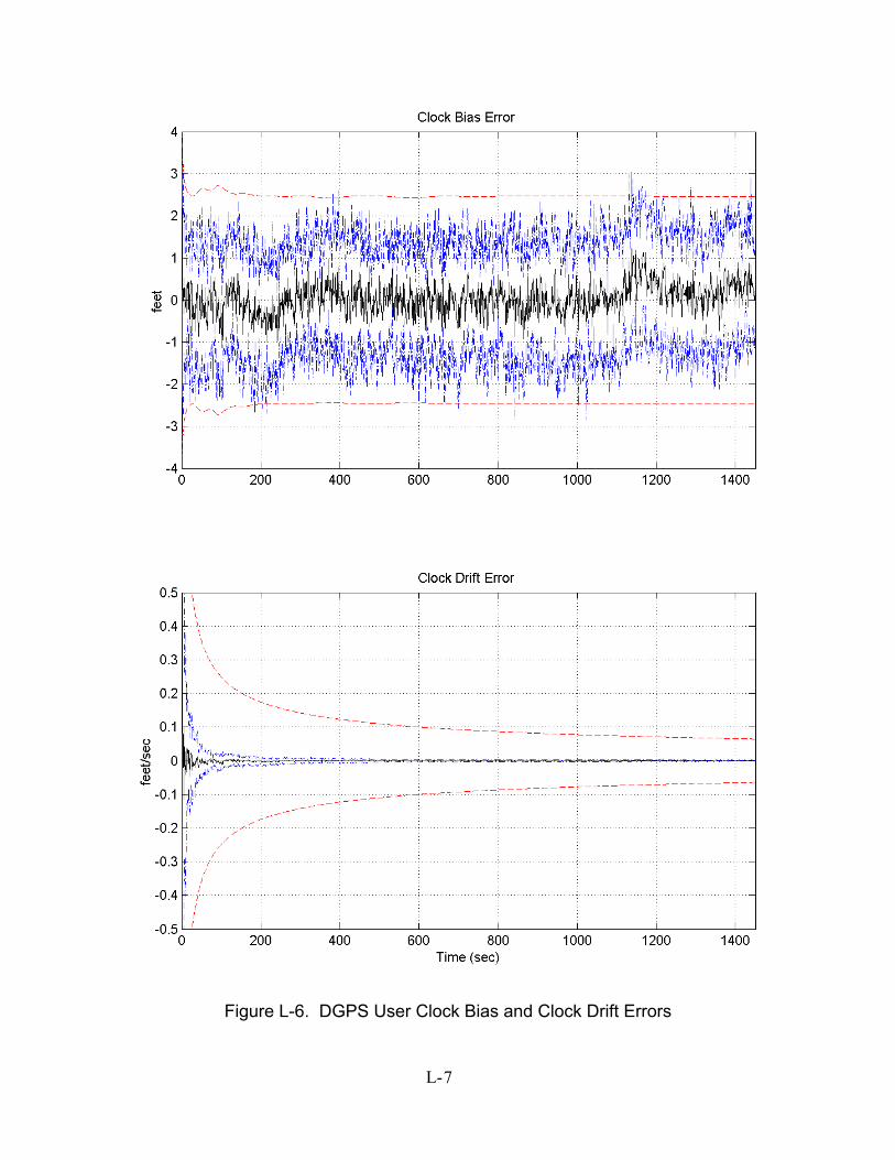
Figure L-6. DGPS User Clock Bias and Clock Drift Errors
L- 7

Appendix M. Plots of Case V
Plot legend:sample mean error
…… true error (sample mean error )
------ filter-predicted error (0 )
trueσ±
filterσ±
M- 1
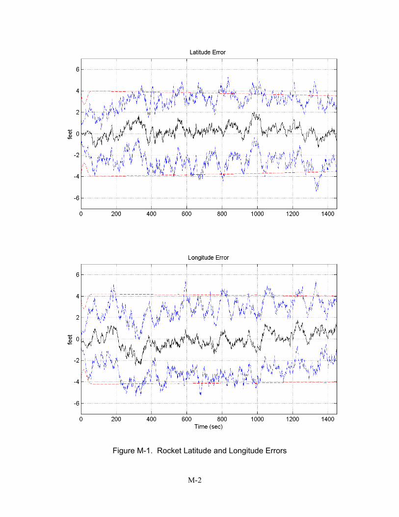
Figure M-1. Rocket Latitude and Longitude Errors
M- 2
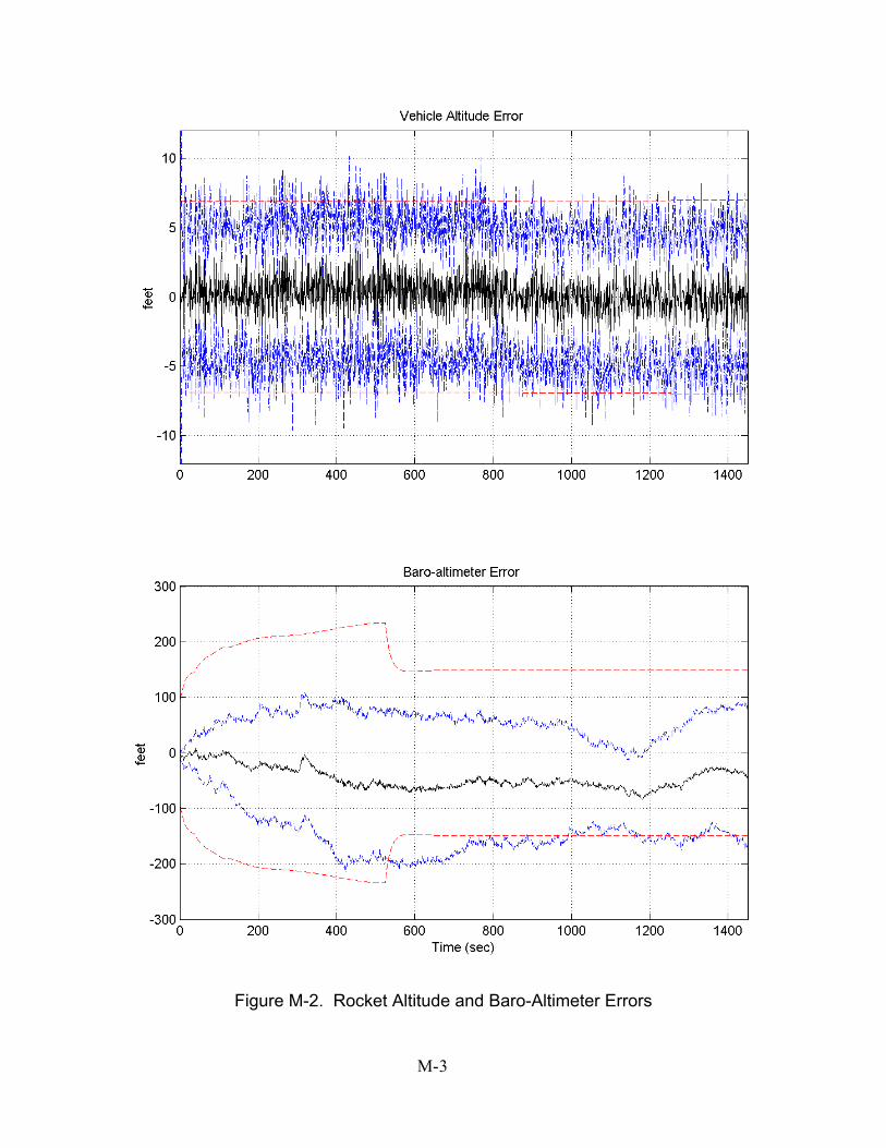
Figure M-2. Rocket Altitude and Baro-Altimeter Errors
M- 3
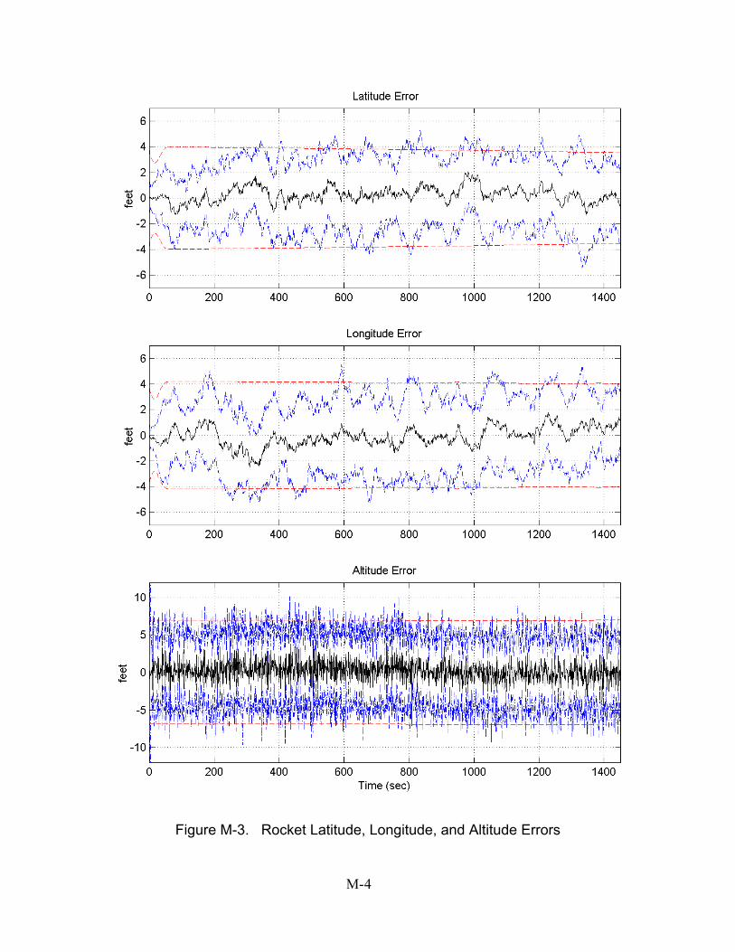
Figure M-3. Rocket Latitude, Longitude, and Altitude Errors
M- 4
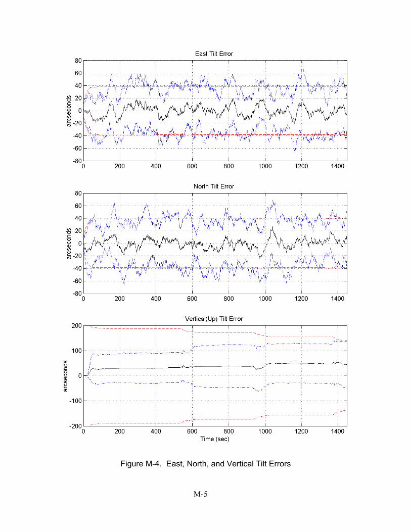
Figure M-4. East, North, and Vertical Tilt Errors
M- 5
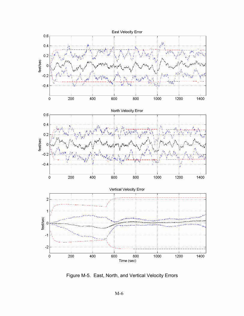
Figure M-5. East, North, and Vertical Velocity Errors
M- 6
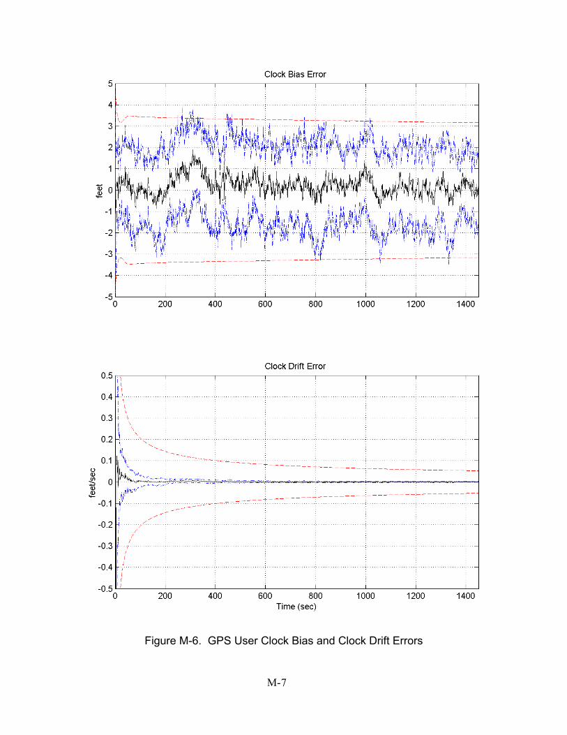
Figure M-6. GPS User Clock Bias and Clock Drift Errors
M- 7

Appendix N Plots of Case VI
Plot legend:sample mean error
…… true error (sample mean error )
------ filter-predicted error (0 )
trueσ±
filterσ±
N- 1
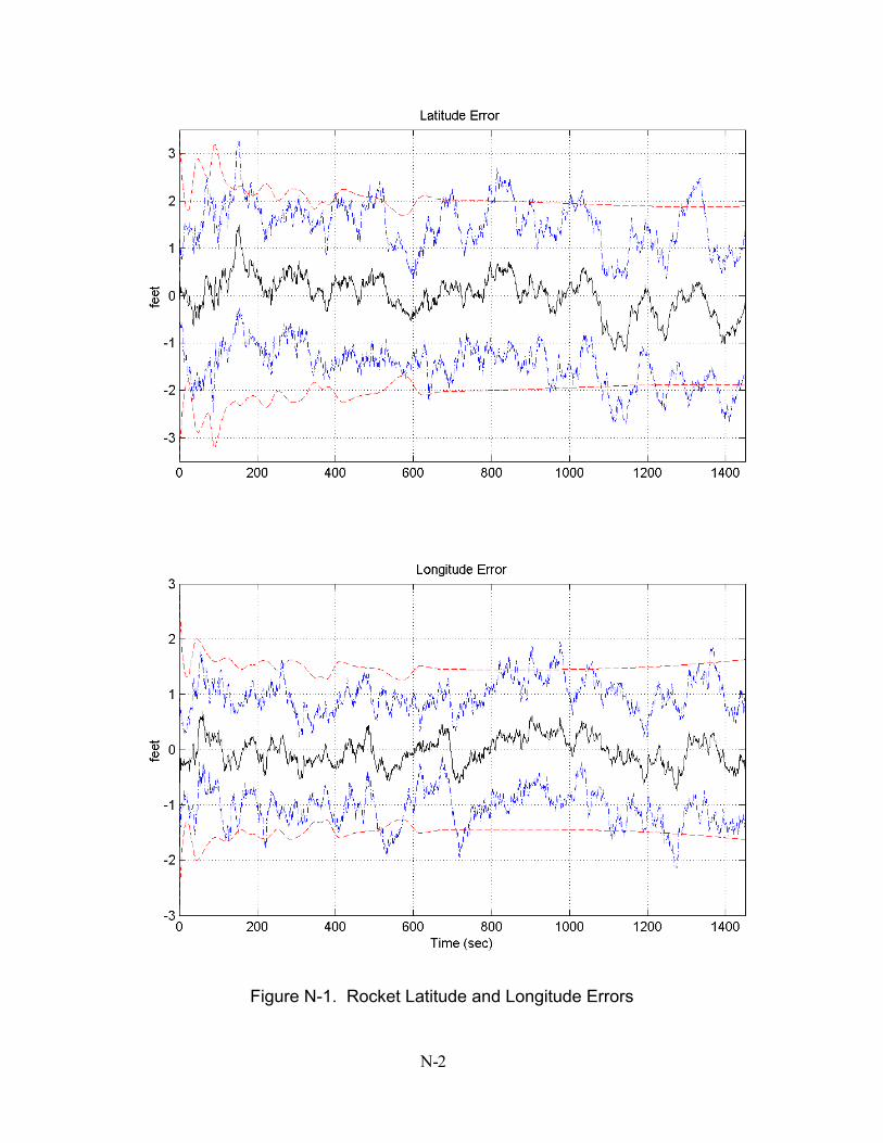
Figure N-1. Rocket Latitude and Longitude Errors
N- 2
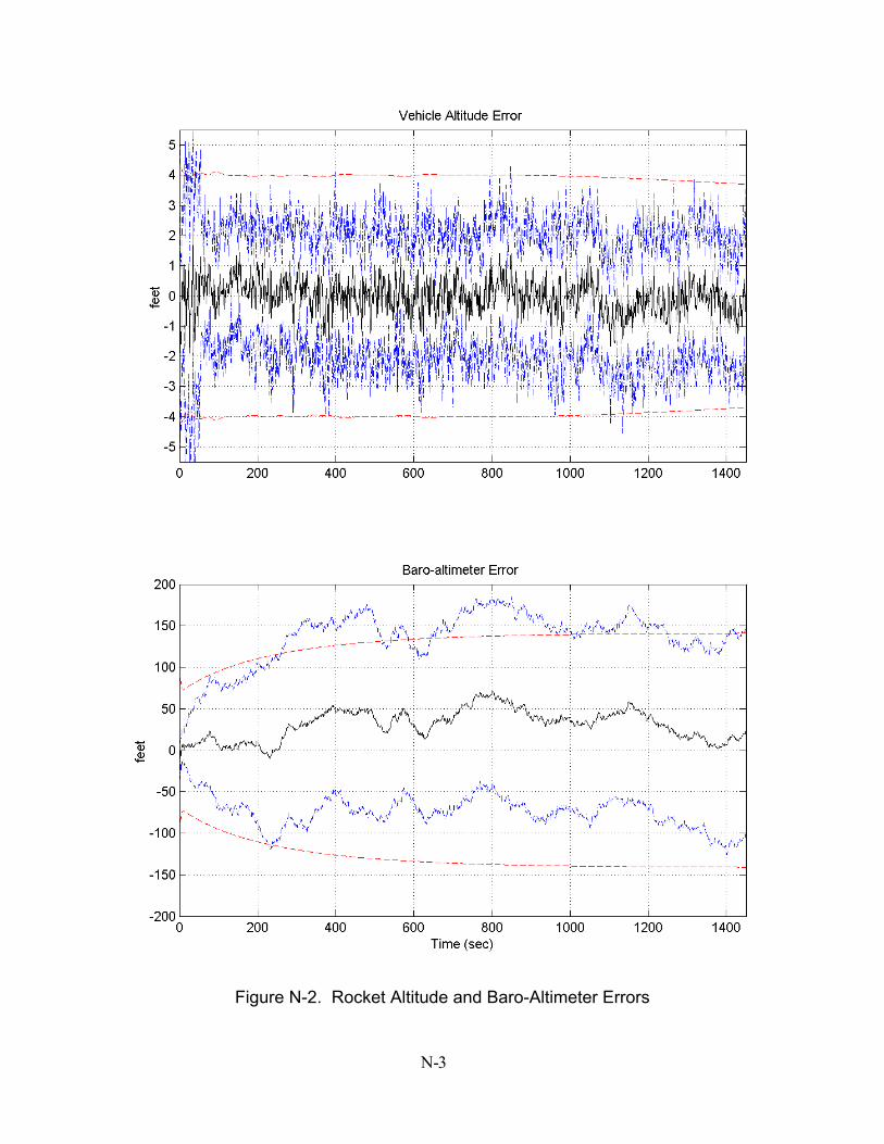
Figure N-2. Rocket Altitude and Baro-Altimeter Errors
N- 3
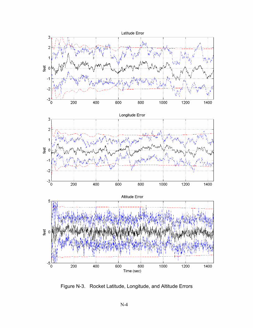
Figure N-3. Rocket Latitude, Longitude, and Altitude Errors
N- 4
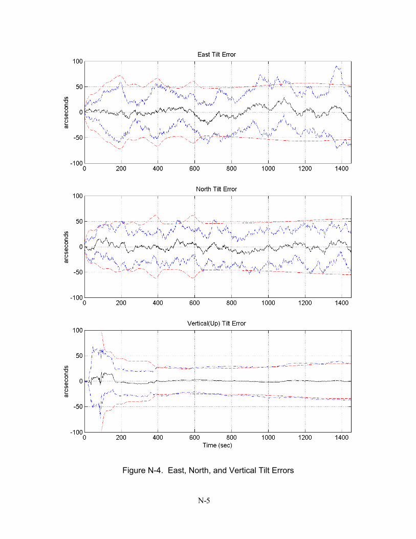
Figure N-4. East, North, and Vertical Tilt Errors
N- 5
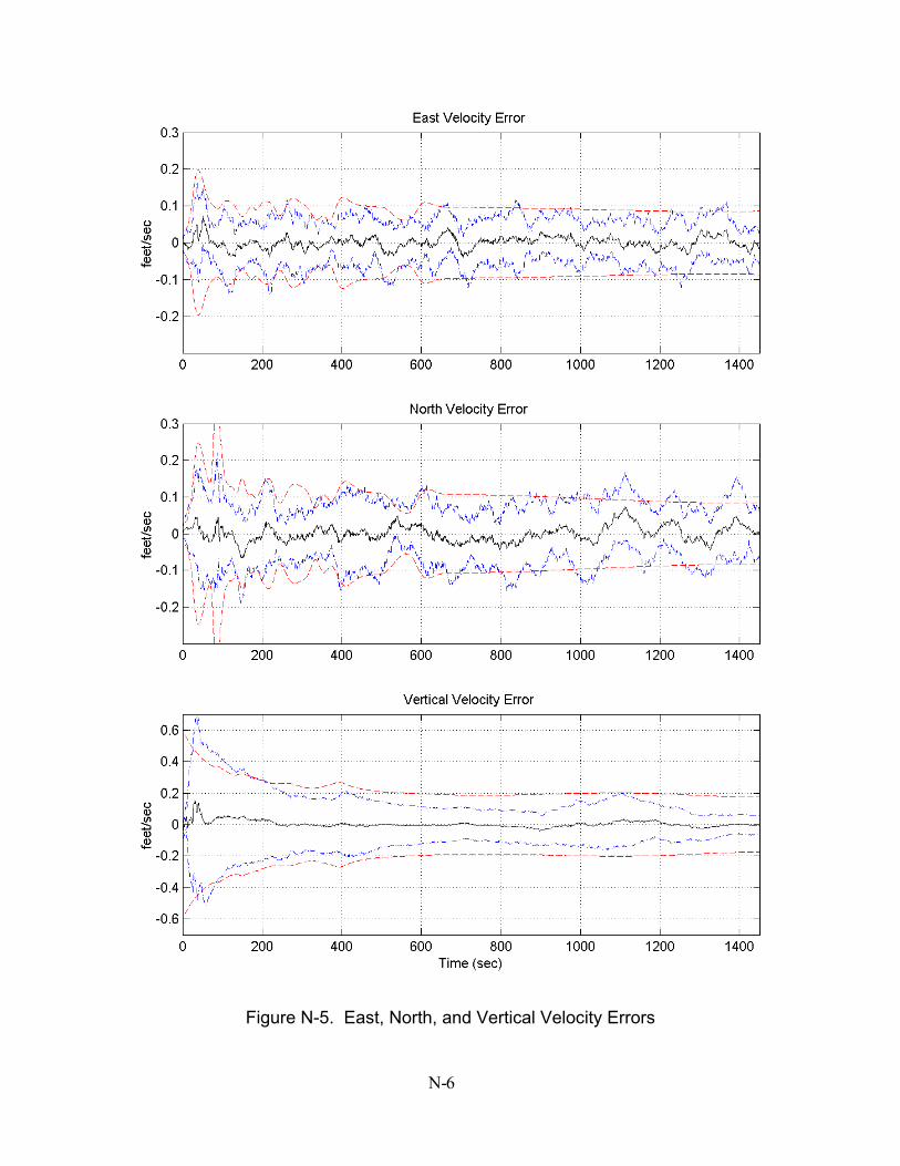
Figure N-5. East, North, and Vertical Velocity Errors
N- 6
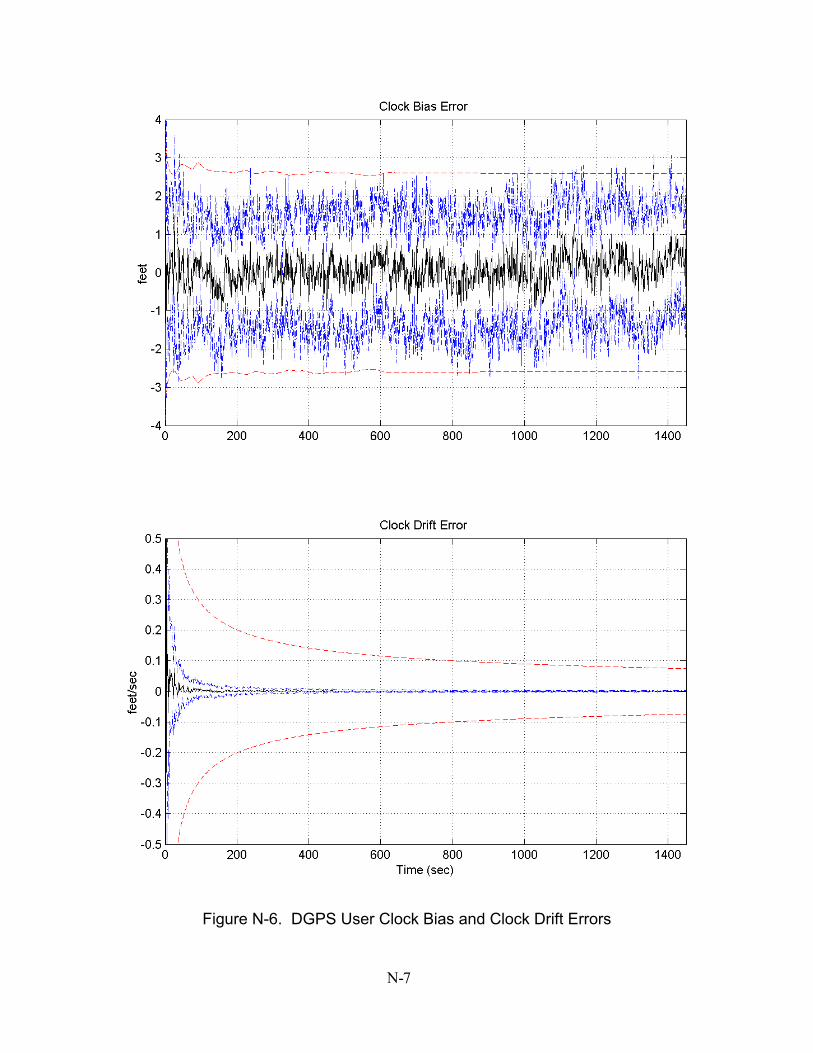
Figure N-6. DGPS User Clock Bias and Clock Drift Errors
N- 7
Bibliography
1 Altmayer, Christian and Sven Martin. “Autonomous Onboard Orbit and Attitude Control of Geostationary Satellites Using Pseudolites,” Proceedings of the11th International Technical Meeting of the Satellite Division of the Institute of Navigation, Nashville, Tennessee, 1565-1578, September 15-18, 1998.
2 ARINC, Inc. “Global Positioning System, Single-Location User System Effectiveness Model Demonstration Software for Windows (WSEM), Version 3.6.4.”, Reference Manual, San Diego, CA, January 2000. http://www.arinc.com/ http;//www.arinc.com/Products_Services/gpsstat.html
3 Bagley, Daniel T. GPS/INS Integration for Improved Aircraft Attitude Estimates. MS Thesis, AFIT/GE/ENG/91D-04. School of Engineering, Air Force Institute of Technology, Wright-Patterson AFB OH, December 1992 (AD-A243947).
4 Braden, Kevin, et al. “Integrated Inertial Navigation System/Global Positioning System (INS/GPS) for Automatic Space Return Vehicle,” IEEE/AIAA/NASA Digital Avionics Systems Conference, 9th,” Virginia Beach VA, 409-414, October 15-18, 1990.
5 Britting, Kenneth R. Inertial Navigation Systems Analysis. New York: Wiley-Interscience, 1971.
6 Britton, Ryan, L. A Differential GPS-Aided INS for Aircraft Landings. MS Thesis, AFIT/GE/ENG/95D-O3, School of Engineering, Air Force Institute of Technology, Wright-Patterson AFB, OH, December 1995 (AD-A306008).
7 Carvalho, H., et al. “Optimal Nonlinear Filtering in GPS/INS Integration,” IEEE Transactions on Aerospace and Electronics Systems, 33: 835-850 (1997).
8 Clark, Fred D. and Ann Christofferson. Applicability of Relative GPS to Automated Rendezvous Between the Space Shuttle and Space Station. NASA Technical Reports, Jan 01,1991, DID No. 19930013052 N (93N22241).
9 Department of the Air Force. NAVSTAR GPS USER EQUIPMMENT. MZI0298.001, US Air Force Space Systems Division, NAVSTAR-GPS Joint Program Office, Los Angeles, CA. February 1991.
10 Gray, Robert A. An Integrated GPS/INS/BARO and Radar Altimeter System for Aircraft Precision Approach Landings. MS Thesis, AFIT/GE/ENG/94D-13. School of Engineering, Air Force Institute of Technology, Wright-Patterson AFB, OH, December 1994 (AD-A289280).
1 BIB-
11 Griffen, Gordon, C. Evans, R. Gray, B.J. Bohenek, The Creation and Validation of a Matlab Tool as a Possible Alternative to MSOFE-Final Report, AFIT Course EENG-735, Air Force Institution of Technology (AFIT), Air Education and Training Command, WPAFB, Ohio, 3 June 1994.
12 Harms, Pamela L. MatSOFE Modifications. Sverdrup Technologies, Inc., TEAS Group. Task Order Number: YH-941531. TEAS Reference Number: 9500202-60U. Eglin AFB, FL, January 1995.
13 Hein, G. W., and M. M. Ertel High-Precision Aircraft Navigation Using DGPS/INS Integration, Institute of Astronomical and Physical Geodesy (IAPG), University FAF Munich, Neubiberg, 1993.
14 Institute of Electrical and Electronics Engineers. IEEE Standard Dictionary of Electrical and Electronics Terms. IEEE Std. 100-1972. New York, NY, 1972
15 Isakowitz, J. Steven, et al. INTERNATIONAL REFRENCE GUIDE TO SPACE LAUNCH SYSTEMS (3rd Edition). Reston, Virginia: AIAA Technical Publications, 1999.
16 Kalman R. E. “A New Approach to Linear Filtering and Prediction Problems,” Transactions ASME, Series D: Journal of Basic Engineering, Vol. 82, 35-45 (March 1960).
17 Kim, Jinwon, et al. “A Complete GPS/INS Integration Technique Using GPS Carrier Phase Measurement,” IEEE Position Location and Navigation Symposium. 526-533 (April 1998), IEEE Cat. No. 98CH36153.
18 Knudsen, L. Performance Accuracy (Truth Model/Error Budget) Analysis for the LN-93 Inertial Navigation Unit. Technical Report, Litton Guidance and Control Systems, Woodland Hills, CA: January 1985. DID No. DI-S-21433 B/T: CDRL No. 1002.
19 Lockheed Martin Corporation web site. “Launch vehicles – Atlas”. January 2002. http://www.lockheedmartin.com/factsheets/product383.html. http://www.ast.lmco.com/launch_atlas.shtml
20 Maybeck, Peter S. Stochastic Models, Estimation and Control. Volume 1. New York: Academic Press. Inc., 1979. Republished, Navtech, Alexandria, Virginia, 1994.
21 Maybeck, Peter S. Stochastic Models, Estimation and Control. Volume 2. New York: Academic Press. Inc., 1982. Republished, Navtech, Alexandria, Virginia, 1994.
2 BIB-
22 Maybeck, Peter S. Stochastic Models, Estimation and Control. Volume 3. New York: Academic Press. Inc., 1982. Republished, Navtech, Alexandria, Virginia, 2001.
23 Miller, Mikel M., Course handouts, EENG 735, Inertial Navigation Systems Analysis and Integration. School of Engineering and Management, Air Force Institute of Technology, Wright-Patterson AFB OH, Spring Quarter 2001.
24 Milliken, R.J., and C.J. Zoller. "Principle of Operation of NAVSTAR and System Characteristics," Global Positioning System, The Institute of Navigation, Vol. I Alexandria, VA, 1980.
25 Misra, Pratap and Per Enge., GLOBAL POSITIONING SYSTEMS Signals, Measurements, and Performance. Lincoln, Massachusetts: Ganga-Jamuna Press, 2001.
26 Moreau, Michael C., and Penina Axelrad. “GPS Receiver Architecture and Expected Performance for Autonomous Navigation in High Earth Orbits”, Journal of The Institute of Navigation, Vol.47, No.3, 191-204, Fall 2000.
27 Mosle, William B. Detection, Isolation, and Recovery of Failures in an Integrated Navigation System. MS Thesis, AFIT/GE/ENG/93D-28. School of Engineering, Air Force Institute of Technology, Wright-Patterson AFB OH, December 1993 (AD-A274056).
28 Musick, Stanton H., “PROFGEN – A Computer Program for Generating Flight Profiles”, Technical Report, Air Force Avionics Laboratory, WPAFB, OH, November 1976. AFAL-TR-76-247, DTIC AD-A034993.
29 Musick, Stanton H., “User’s Guide for PROFGEN (A Flight Profile Generator)”, AFRL Technical Memorandum, WPAFB, Ohio, June 2001
30 Musick, Stanton H., and Neil Carlson. User's Manual for a Multimode Simulation for Optimal Filter Evaluation (MSOFE). AFWAL-TR-88-1138, Wright-Patterson AFB OH: A.F. Avionics Laboratory, AFWAL/AARN-2, April 1990.
31 Musick, Stanton H. Electronics Engineer, WL/AAAS-3, Air Force Avionics Laboratory, WPAFB, OH. Personal telephone conversations. Winter 2002
32 National Geodetic Survey(NGS)’s Continuously Operating Reference Stations (CORS) web page. “Global Positioning System (GPS) carrier phase and code range measurements in support of 3-dimensional positioning activities throughout the United States and its territories”. Winter 2001. http://www.ngs.noaa.gov/CORS/
3 BIB-
http://www.ngs.noaa.gov/CORS/download1/ http://www.ngs.noaa.gov/CORS/download2/
33 Negast, William Joseph. Incorporation of Differential Global Positioning System Measurements Using an Extended Kalman Filter for Improved Reference System Performance. MS Thesis, AFIT/GE/ENG/91D-41. School of Engineering, Air Force Institute of Technology, Wright-Patterson AFB OH, December 1991 (AD-A243742).
34 Raquet, John F. Course handouts, EENG 533, Navigation Using The GPS. School of Engineering and Management, Air Force Institute of Technology, Wright-Patterson AFB OH, Spring Quarter 2001.
35 Sabatini, Roberto (Italian Air Force). High Precision DGS and DGPS / INS Positioning for Flight Testing. NASA Technical Reports, 6th Saint Petersburg International Conference on Integrated Navigation Systems, 18-1 – 18-17, Oct 01, 1999, DID No. 2000001219.
36 Stacey, Richard D. A Navigation Reference System (NRS) Using Global Positioning System (GPS) and Transponder Aiding. MS Thesis, AFIT/GE/ENG/ 91M-04. School of Engineering, Air Force Institute of Technology, Wright-Patterson AFB OH, March 1991 (AD-A238890).
37 The MathWorks, Inc. “MATLAB, The Language of Technical Computing”, Version 6.0, Winter 2001. http://www.mathworks.com/
38 The United States Coast Guard web site. “Navigation Center (navcen)” http://www.navcen.uscg.mil/gps/almanacs/default.htm.
39 Tragesser, Steven G. Assistant Professor of Aerospace Engineering, Air Force Institute of Technology, Wright-Patterson AFB OH. Personal interview. 18 Jan 2002.
40 Upadhyay, Triveni N., et al. Autonomous Integrated GPS / INS Navigation Experiment for OMV: Phase 1 Feasibility Study, NASA Technical Reports, NASA- CR- 4267, Jan 01, 1990, DID No. 19900011653 N (90N20969), Contract No. NAS8-38931.
41 Upadhyay, T. N. “Autonomous GPS/INS Navigation Experiment for Space Transfer Vehicle,” IEEE Transactions on Aerospace and Electronics Systems, 29: 772-785 (1993).
42 Varner, Christopher and Elizabeth M. Cannon. “The Effects of Altitude on GPS Dilution of Precision and Coverage”. Proceedings of the 51st Annual ION Meeting, Colorado Springs, Colorado,119-127, June 5-7, 1995.
4 BIB-
5 BIB-
43 Vasquez, Juan R. Detection of Spoofing, Jamming, or Failure of a Global Positioning System (GPS). MS Thesis, AFIT/GE/ENG/92D-37. School of Engineering, Air Force Institute of Technology, Wright-Patterson AFB OH, December 1992 (AD-A259023).
44 White, Nathan Alan. MMAE Detection of Interference/Jamming and Spoofing in a DGPS-Aided Inertial System. MS Thesis, AFIT/GE/ENG/96D-21, School of Engineering, Air Force Institute of Technology, Wright-Patterson AFB, OH, December 1996 (AD-A320882).
45 Williams, W., et al. “A Comparison of State Space, Range Space, and Carrier Phase Differential GPS/INS Relative Navigation,” Proceedings of the 2000 American Control Conference. Volume 4, 2932-2938, Chicago: IEEE Press, 2000, IEEE Cat. No. 00CH36334.