Aigorithms for the Kinematic Control of Redundant...
120
J , Aigorithms for the Kinematic Control of Redundant Manipulators Saumyendra Mathur Bachelor of Marine Engineering (Directorate of Marine Engineering Training. Calc.utta. India). 1986 Department of Mechanical Engineering McGill University Montréal. Canada A thesis submitted to the Faculty of Graduate Studies and Research in partial fulfillment of the requirements for the degree of Master of Engineering July. 1989 © Saumyendra Matour
Transcript of Aigorithms for the Kinematic Control of Redundant...
J
,
Aigorithms for the Kinematic Control of Redundant Manipulators
Saumyendra Mathur
Bachelor of Marine Engineering (Directorate of Marine Engineering
Training. Calc.utta. India). 1986
Department of Mechanical Engineering
McGill University
Montréal. Canada
A thesis submitted to the Faculty of Graduate Studies and Research
in partial fulfillment of the requirements for the degree of
Master of Engineering
July. 1989
© Saumyendra Matour

1
To
my fam"y
ii
1
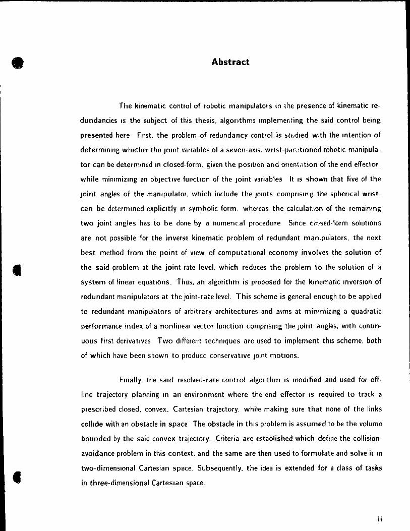
Abstract
The kinematic control of robotie manipulatofs in the presence of kinematic re
dundancies IS the subject of this thesis. algonthms Implementing the said control being
presented here Flrst. the problem of redundancy control is ~tl'\(I\~led wlth the Intention of
determining wh ether the jOint variables of a seven-axis. wrrst-pdrutloned robotlc manipula
tor can be determlned 10 closed-form. given the position and orlen\\ition of the end effector.
while minlmizmg an objective functlon of the Joint variables It IS \;hown that five of the
Joint angles of the manlpulatar. which include the JOints eomprtsm\,~ the sphencal Wrlst.
can be determmed explieltly ln symbolic farm. whereas the calculakln of the remainmg
two joint angles has to be done by a numencal procedure Smce ck .. sed-form solutIOns
are not possible for the inverse kinematic problem of redundant mampulators. the next
best method from the point of vlew of computatlonal economy involves the solution of
the said problem at the joint-rate level. which reduces the problem to the solution of a
system of linear equatlons. Thus. an algorithm is proposed for the kmematic inversIOn of
redundant m<lnipulators at the joint-rate level. This scheme is general enough to be applled
to redundant manipulators of arbitrary architectures and alms at minimizmg a quadratic
performance index of a nonlinear vector function compnslng the Joint angles. wlth con tm
uous first derivatlves Two dlfferent techniques are used to implement thls scheme. both
of which have been shown to produce conservatlve JOint motions.
Final/y. the sald resolved-rate control algonthm 15 modified and used for off
line trajectory planning ln an environment where the end effector IS required to track a
prescribed closed. convex. Cartesian trajectory. while making sure that none of the links
coillde with an obstacle in space The obstacle in thls problem is assumed ta be the volume
bounded by the sa id convex trajectory. Criteria are established which defme the collision
avoidance problem in this context. and the same are then used to formulate and solve it ln
two-dimenslonal (artesian space. Subsequently. the idea is extended for a class of tasks
in three-dimensional Carteslan space.
iii
1 Résumé
Le sujet de cette thèse est la commande des mampulateurs robotiques en
présence de redondance cinematique, des algorithmes utilisés à cette tin étant obtenus
et réalisés, D'abord, le problème de commande en présence des redondances est étudié
dans le but de déterminer SI les variables articulaires d'un manipulateur à sept articulations
dont les troIs derniers axes sont crOIsent peuvent être obtenues symboliquement. la POSI
tion et l'orientation de l'organe terminai étant donnés, tout en minimisant une fonction des
variables articulaires Il est montré que cinq des variables, incluant celles des articulations
du pOignet, peuvent être détermmées explicitement sous forme symbolique, alors que les
deux autres variables dOIvent être obtenues numériquement PUlsqu'll n'est pas possible
d'obtenir des solutions symboliques pour le problème de cinématique inverse des mainpu
lateurs redondants. la méthode la plus efficace du pOint de vue informatique vise à une
solution au niveau des vitesses artICulaires Un tel pfoc~d; est économique en temps de cal
cul par rapport aux méthodes Itératives pUisqu'II s'agit seulement de résoudre un système
d'équatIOns linéaires, tel que proposé ICI Cette méthode est suffisamment générale pour
être appliquée à des manipulateurs redondants à architecture arbitraire, ayant pour but
la mlnlmizatlon d'une fonction quadratique des vartables artICulaires, à dérivées premières
continues Deux techniques différentes sont utilisées pour résoudre ce système, toutes
deux prodUisant des mouvements conservatlfs au niveau des articulations
Finalement, cette méthode est modifiée pour l'utiliser hors ligne pour prédetermi
ner des trajectOires d'articulations dans un envlronement ou l'organe terminai doit suivre
une trajectoire cartésienne convexe et fermée, tout en s'assurant qu'aucun des membres ne
rencontre un obstacle, Dans ce prob'~me, l'obstacle est défini comme la region enfermée
par la trajectoire convexe, Des cntères de collision sont deflnls. et ultérieurement utilisés
pour formuler et résoudre le problème dans un espace cartésien à deux dimensions, En
suite. l'idée est généralisée pour une famille de tâches dans un espace cartésien à trois
dimensions,
iv
c
c
Acknowledgements
1 would like to thank Professor Jorge Angeles for the guidance and inspiration
that he provided for thls research
1 am very much grateful to my parents for their support and en(.ouragement.
Many thanks are due ta the patient and helpful students of the McGili Research
Centre for Intelligent Machines. 1 am indebted to Meyer Nahon for hls invaluable help in
generattng the computer anlmatton on the IRIS™ workstatlOn and translating the abstract
1 am grateful to Messrs Gregory loannides. Subir Sa ha and Ou Ma for the many frUltful
discussions we had during the course of my research. Thanks to Messrs. Ronald Kurtz
and Joshua Pina for their help ln drawing the figures.
1 am grateful to Ms Helga Symington for photographing the computer frames.
Due thanks ta the McGill Research Centre for Intelligent Machines for the stim
ulating research envlronment and the invaluable technieal support.
The research work reported here was possible under NSERC (Natural Sciences
and Engineenng Research Couneil. of Canada) Grant No. A4532. and FCAR (Fonds pour
la formation de chercheurs et raide à la recherche. of Quebec) Grants No. EQ3072 and
No. 88AS2517.
v

Contents
List of Figures VII
L,st of Tables. IX
Claim of O"gma/ity . .. . 1
Chapter 1 Introduction. . ............... 2
1.1 Robots and Redundancy .............. 2
1 2 Inverse Kinematlcs of Redundant Mantpulators . . ............. 4
1.3 ObjectIVe and Motivation ..... 9
1.4 Orr.anizatlOn of the thesis .... 10
Chapter 2 Background and Terminology ..... . .. , ........ 12
2.1 H artenberg- Denavit Nomenclature . .... . . . ....... ...... 12
2.2 Rigid-Body Motions .. . . . ... .... .. 14
2.3 KlOematic Closure Equations 15
Chapter 3 On the Search of Closed- Form Solution ta the
IKP .. 17
3 1 Inverse kinematics ... 17
3.1.1 Posltionmg .. . . . . . . .. 18
3.2 Example. .... . .... .. ..... 31
Chapter 4 A Resolved-Rate Control Aigorithm. . .. ............... 33
4.1 Introduction..................................................... 33
4.2 Resolved-Rate Schemes for the Kinematic Inversion of Redundant
Manipulators. . . . . . . . . . . . . . . . . . . . . . . . . . . . . . . . . . . . . . . . . . . . . . . . . . . .. 34
4.3 Examples ...................................................... 43
vi
4.3.1 Example 4.1 : A Redundant Planar Positioning Manipulator ..... " 43
4.3.2 Example 4.2 : A Redundant Planar Positioning Manipulator. ..... 45
4.3.3 Example 4.3 : Seven-Axis Path Tracing Mampulator. . . . . . . . . . . . .. 47
Chapter 5 Complexity Analysis . 51
Chapter 6 Off-Une Trajectory Planning for Collision
Avoidance
6.1 Introduction ............ .
...... 58
58
6.2 Collision AvO/dance with a Planar Manipulator " ... ................. 61
6.2.1 Collision-Avoidance Policy . ......... ..... ..... ..... .... 61
6.2.2 Obstacle-Avoidance Algorithm . . . . . . . . . . . . .. ...... .......... 64
6.3 3-D Obstacle Avoldance with a Seven-Axis Manipulator ... 74
Chapter 7 Conclusions. . . . . . . . . .. ............... ..... ........... 87
7.1 SuggestIons for Future Researc,1. ................ . . . .. .......... 89
References . .. 90
Appendlx A . ....................... , 94
A.l Solution for ()2 ................ . ..................... 94
A 2 Derivation of the constraint equation. . . . ........ 94
Appendix B
Appendix C
Appendix D.
Appendix E.
... ....... . . . . , ...... ................ ........ .. 95
101
103
108
E.l Dertvations for aÀ/ ao . . . . . . . . . . . . . . . . . . . . . . . . . . . . . . . . . . . . . .. 108
E.2 Derivation for ae / ao. ..................... ................ 109
vii
l
1 List of Figures
3.1 Architecture of the Redundant Manipulator ... . . . 18
32 Dt~!>;red confIguratIon for the first joint . - ... ... 19
3.3 Projection of the Mantpulator Imks on the X' r' Plane 20
34 Inner Workspace Boundary of the Mantpulator 22
3.5 Carteslan trajectory 30
3.6 Joint histories .... 32
4.1 EE drift m Cartesian space . . . . . . . . . . . . ~ . 40
4.2 TraJectory traced by pl anar manlpulator . .... o •••••• 43
4.3 Joint histones of the planar manipulator 44
t • 4.4 Joint histones of the pl anar manlpulator . . . . . . . . ... , .. 45
4.5 CYBOTECH P-15 architecture. 47
4.6 Trajectory traced by CVBOTECH P-15 . 48
4.7 Joint histones of CVBOTECH P-15. 49
48 Jomt histones of CV BO TECH P-15 50
6.1 Thlrd Imk farthest From obstacle Obstacle shown as the shaded
reglon ... " . . .. ..... .... .... 62
6.2 Second link tangent to the largest ellipse shown dotted. Ellipse drawn
with solid Ime IS the hypothetîcal boundary of the obstacle. i.e. the
shaded reglon. '" . .... .... ... . 63
6.3 Planar trajectory and obstacle assumed to be an ellipse .... 64
6.4 Manipulator losing a redundant DOF while branch switching . . . . . . . . . . .. 71
- 6.5 Manipulator losing a redundant DOF while branch switching . . . . .. . ... , 71
6.6 Actual and Spline interpolated joint histories ............. ....... ... 72
viii
,
6.7 Actual and Spline interpolated joint histories 73
73
75
76
78
81
82
6.8 Actual and Spline interpolated joint histories
69 PUMA and Its eqUivalent planar architecture
610 CYBOTECH and Its eqUivalent planar architecture
611
6.12
6.13
6.14
6.15
6.16
6.17
6.18
6.19
6.20
6.21
TraJectory ln 3-dlmenslonal Carteslan space , , , .
Actual and spline Interpolated JOint histories . .
Actual and spline mterpolated joint histories .....
Mantpulator configuration at sample point 51 . . . . . . . . . . . . . . . . . . . .. .. 82
Mantpulator configuration at sample point 52 . . . . . . . .. .............. 83
Manipulator configuration at sample point 53 . . . . . . . . . . . . . . . . . . .. ... 83
Manipulator configuration at sample point 54 ...................... " 84
Mampulator configuration at sample point 55 . . . . . . . . . . . . . . . . . . . .. .. 84
Manipulator configuration at sample point 56 ....
Mampulator configuration at sample point 57' .,
Mampulator configuration at sample point 58 ....
6.22 Mantpulator configuration at sam pie pOint S9 ...
85
85
86
86
,
...
'.
List of Tables
3 1 HD parameters of the spatial positioning redundant arm. . . . . . . . . . . . .. . 18
4.1 HD parameters of CYBOTECH P-15 ., ..... ....................... 47
x
1 Claim of Originality
The author of this thesis daims the ongmality of.
1) the discussions and the methodology leadlng to the derivation of the sym
bolic/numerical scheme for the kinematic inversion of a simple. orthogonal.
wrtst-partltloned. seven-Itnk robotic manlpulator.
2) the resolved-rate control algoritnm for the kinematic Inversion of redundant
robotlC manipulators wlth general architectures.
3) the off-line trajectory planning algorithm for collision avoidance.
1
t
Chapter 1 Introduction
1.1 Robots and Redundancy
The word robot usuaUy means different things to different people. In a child.
this word mlght conjure up the images of R2D2. No. 5. or lately Roboeop and Data.
the machines with remarkably human-like charactenstics. popularized by the science-fiction
movies. The origin of this word. however. can be traced to the early twentieth century. when
Karel <:':apek used it in his play Rossum's Untversal Robots. whlch ln Czech means ·serf'.
For an informed person-one who is aware of the state-of-the-art technology-a robot is a
multlfunction. computer-controlled. electro-mechanical device that can be programmed to
perform a variety of tasks
On the other hand. manlpulators were ln existence evell before computer con
trol wa5 introduced Any mechantcal devlce which 15 used to manipulate objects by manual
guidance. through a purely mechanlcal master-slave arrangement. can be termed a mantpu
lator. Such devices have traditlonally found wide applications ln the areas where radioactive
elements. or chemicals that are harmful for human beings. have to be handled. In recent
years. this technology has been very efTectively applied for space applications in the form
of manipulators like the CANADARM. on bO<lrd the space shuttle. The said manipulator
is controlled by an operator inside the shuttle. with the help of a joystick.
Such manipulator5. when operating under computer control are known as ,obotie
1
c
1
1 Introduction
manipula tors. These devices find extensive industrial applications primarily in manufactur
ing. for tasks like picking up objects from the conveyor belt and stacking them in a shelf. a
job which is repetitive and monotonous for human beings. Another area where robots are
being used is where extraordlnary precIsion 15 requlred like ln the wlring of circuit boards.
A typlcal robotic mantpulator contams as a basic component an open or a
c\osed kinematlc chain ln which ail the consecutive links are cou pied to one another by
either a) revolute joints. or b) prismatic joints. A revolute joint imparts a rotational motion
to the adjacent Ilnk. whereas. a prismatic joint provides translational motion A gripper.
commonly referred to as the end-effector (EE). is fixed to the last Itnk of an open chain.
thus completmg the manipulator structure ln thls thesls only open kinematlc chains with
revolute and pnsmatlc joints will be considered.
It has been acknowledged by researchers that a human arm is an ideal manipu
lation device which has developed into Its present form after millions of years of evolutlon.
Consequently. it has been the endevour of roboticists to incorporate its characteristlcs such
as dexterity. versatility and accuracy in robotic devices. Most robotic manipulators have
been designed wlth one or more of these qualitles in mind. One of the prmcipal character
istics of human arm IS that it has kmematlc as weil as actuator redundancies. RoboticIsts
have been striving lately to design manipulators wlth these characteristics (Hayward 1988).
However. thls thesls IS Ilmlted to the study of the kinematlc redundancies only.
If the human arm IS modelled ktnematically ln a very slmphfied manner with
lower pairs. it can be observed that the shoulder comprrses a spherical joint which lends
three degrees-of-freedom (DOF). The elbow contributes only one DOF by supination. and
the wrist provides another three DOF Hence. a human being uses a total of seven degrees of
freedom to pose-position and orrent-the hand in the three-dimensional Cartesian space. a
task for which onl}' six degrees of freedom would suffice. This additional degree of freedom
in the arm is referred to as kinematic redundancy and accounts for the extra versatihty and
dexterity thot is imparted to the limb.
3
1 Introduction
The concept of kinematic redundancy can be further understood by relating
the term task-space dimension to the degrees of freedom of the manipulator Task-space
dimension IS defmed as the minimum number of DOF required by a manipulator to perform
a specified task For example. posltloning a pOint on curve. or. onentmg a rigld body
about an axis requires only one DOF and hence the task-space dimension. rn. IS 1. A two
dimenslonal task-space is assoclated with the posltlOnmg of a pOint in a plane. whereas
three-dimenslonal task space IS needed for posltlonmg a pomt ln 3-dimensional Cartesian
space or onenting a rigid body in the same space Similarly. a task space of dimension SIX
is essential if a rigid body has to be arbitrarily positioned and oriented ln three-dimensional
Cartesian space If the mampulator performing one of the above mentlOned tasks has
n degrees of freedom such that 7/ > m. then It IS said to be kinematlcally redundant.
Normally. a three-degree-of-freedom planar mampulator IS not ca/led redundant if the alm
is to position and orient the gripper ln the plane If the intention is to disregard the
orientation and concentrate only on positionmg the end efTector in the plane. then. the
manipulator becomes redundant for that particular task.
The idea of designing robotic manipulators with kinematlc redundancles germi
nated wlth the need for prosthetic devlCes to replace the amputated limbs (Whitney 1972).
Since then. a substantlal amount of research effort has been concentrated ln thls field. A
milestone ln thls research will be reached when the Mobile ServlCing System (MSS) IS fully
operatlonal in the proposed space-statlon MSS will have a redundant architecture wlth a
total of 23 degrees of freedom It Will be instrumental ln the assembly of the space station
structure and later will be used for a vanety of tasks IIke general maintenance. dockmg of
the shuttles. helpmg the astronauts perform extra-vehlcular actlvltles. etc
A brief survey of the research conducted m the domain of the kinematic mversion
of redundant manipulators IS presented ln the next sub section
1.2 Inverse Kinematics of Redundant Manipulators
Inverse kinematics is defined as the mapping of the Cartesian coordinates of a
4
1
1
1 Introduction
given link of the manipulator. usually the EE. into the joint coordinates of the manipulator.
This study forms the backbone of robotle applic:ations. In the nascent stages of robotics
the study of inverse kmematics was IImited to that of non-redundant manipulators. T 0
date researchers are still attempting to discover ail the possible solutions to the inverse
kinematlc problem (IKP) of non-redundant mantpulators with arbitrary architectures and
propose effiCient algorithms for the computation of the same. In thls respect. mention
should be made of Pleper (1968) who noted that manipulators wlth partlcular architectures
facilltated the solution of the Inverse klnematlc problem in closed form. By closed form It
is meant that the JOlOt angles can be computed by a set of cascading equations quadratic
or quartic in the joint caardlnates.
Primrose (1986) proved that the inverse kinematic problem of a six-axis non
redundant manipulator of arbltrary architecture admits up to sixteen solutions. Much of
the subsequent research was eoncentrated on finding these sixteen solutions. as indlcated
by the literature survey in Williams (1989). As opposed to the case of non-redundant
manipulators. the Inverse krnematic problem of redundant manlpulators. in general. admits
an infinrte number of solutions known as homogeneous solutions Thus. the choice of a
partlcular solution becomes Important and various schemes have been devised for the sa me.
These schemes have been largely based on the fact that the redundancy in the kinematic
structure allaws for eompliance with a secondary objective such as'
• Ltmiting Joint velocitœs (Fisher 1984):
• Mlmmizing kinetlc energy (Whitney 1972):
~ Avoidmg singulaflties (Luh and Gu 1985. Angeles 1988):
• Minimizing Joint torques (Hollerbach and Suh 1985):
• Improving manipulability (Yoshlkawa 1985):
• Task-priority-based control (Nakamura et al. 1987):
5
1
1 Introduction
• Obstacle avoidance (Maciejewski and Klein 1985):
• MinimizatÎon of energy consumption (Kazerountan 1987);
• etc
The general methodology adopted for findmg a solution to the inverse kinematic
problem of redundant manlpulators. while allowmg for the satisfaction of a secondary objec
tive. involves the solvmg of a nonhnear-programming problem ln broad terms. the schemes
for the kmematie mverslon of robotie mampulators can be dlvided lOto two groups ln the
first one. the JOint-histones are eomputed at the Joint-coordinate level; ln the second. the
jOint rates are obtamed f"st. and then the JOint coordinates are determined by integration.
The latter group leads to schemes known as resolved-rate control. For real tlme applica
tions closed-form solutions appear attractive. However. to the author' s knowledge no one
has been able to denve optimum closed-form solutions for redundant manipulators, similar
to the ones derived by Peiper (1968) for the inverse klnematlc solution of non-redundant
manipulators Hollerbach (1985) proposed the expliclt symbolic kinematic inversion of 7-
DO F mampulators of two dlfferent architectures. but these solutions do not permit the
optimlzation of any performance Index. Stani~ié and Pennock (1985) succeeded ln deter
mlning a non-degenerate solutIOn to the Inverse kinematlc. problt>m of a manlpulator wlth
redundant wnst. In closed form. Chang (1986) solved the mverse klnematlc problem by
adoptlng the Lagrange multiplier techntque HIS algonthm IS vahd for redundant mampu
lators with general architectures and allows the optlmlzatlon of an objective functlon. The
main feature of thls algonthm 15 that the values of the JOint angles can be computed by sim
ply solvlng a determmed system of equatlons, whlch IS more efficient than the technique
of evaluating the pseudoinverse of the Jacobian (Whitney 1972, Liégeois 1983). In any
case, the computation of the pseudomverse by invertmg the mampulator Jacoblan matnx
times its transpose must be avoided because the resultmg square matnx, whose inverse is
needed. IS frequently III-condltioned One methud avoldlng the explicit inversion of JJT, J
being the m i' n manlpulator Jacoblan, IS that propounded by Dubey et al (1988) for the
kinematic inversion of a seven-axls robot wlth sphencal wrists. Their mode of formulation
6
t
t
1 Introduction
results in the evaluation of the joint rates by the solution of two sets of three simultaneous
equations. These authors tested the algorith m on the CESAR research manipulator.
An important aspect of the resolution of the kinematic redundancles. from the
vlewpoint of computatlonal efflclency. is the technique used for optlmlzmg the performance
index subject to the constramts ln this context. the work by Yah~1 and Ozg6ren (1984)
should be mentloned. \Nho used the Oavidon- Fletcher-Powell optlmlzatlOn procedure (Man
gasarian 1972) for solvlng the nonlmear programming problem This method. however.
requires the introduction of Lagrange multipllers. thereby Increasmg the dimension of the
problem. Later. Angeles et al. (1987) proposed two methods for solving the mverse kine
matie problem of redundant manlpulators at the joint-coordinate level. the flrst of whlch IS
based on the least-square approXimation of an overdetermined nonhnear system of equa
tions ln thls method. the objective function IS quadratic ln the nonlmear vector function
of the joint variables Thelr second method. termed the approach-descent method. does
not require that the objective function be quadratic. as in the tlrst method. Ali it requires
is that the performance index have contmuous first-order derivatives. Goldenberg et al
(1985) proposed a modifled Newton-Raphson iteratlve scheme whlch can be used for the
kmematlc inversion of redundant as weil as non-redundant manipulators of arbitrary archi
tectures Benatl et al (1982) proposed an Inverse kmematlc algorithm for anthropomorphic
manipulators. but It avoids the optintlzatlon of a performance mdex.
Any optimlzation method that deals wlth the Inverse kmematic problem at the
jomt-coordmate level has the inherent drawback of bemg computatlonally expenslve. as
compared to an a Igonthm that deals with the same problem at the Jomt-rate level. However.
one cannot totally disregard the former. since it is used to generate the joint values at the
startmg point of the trajectory. to enable the tracking of the path to be performed at the
Joint-rate level. Whitney (1972) was the tirst researcher who used resolved-rate control for
the kinematic inversion of redundant manipulators The formulation he proposed is given
as. • J.
O=Jx (1.1 )
7

1
1
r
1 Introduction
where Jt is the pseudoinverse of the manipulator Jacobian. computed as:
(1.2)
Addltlonally. he clalmed that pseudolnverse control would automatlcally result in manipu
lator configurations which would be away from singulaflties He based thls argument on
the fact that the kinematlc smgularities are characterized by high Joint rates. and slnce
the pseudoinverse formulation IS eqUivalent to mlnlmlzlng il quadratlC function of the JOint
rates subject to the dlfferential relation between the EE Cartesian velocity and the jOint
rates. the singularttles will be avolded. However. 8aillieul et al (1984) pointed out that
thls argument IS speclous. and the singularities are not avoided by this technique. In any
practical sense.
LiégeoIs (1975) presented an alternate method for the resolved-rate control
which involves the optimization of an additional cnterion. This modified scheme is of the
form given below.
(1.3)
where Jt is agaln the pseudoinverse of the Jacoblan as given in eq. (1.2). z. i and l being
an optimizatlon criterion. an rn-dlmensional vector of Carteslan velocit,es and the n x n
Identlty matrlx. respectively It should be noted that ::: is il function of the Joint coordinates
and that [1 - l JJ\'.:: represents the projection of \'::: Into the null space of JT. which
should be zero for the first-order normallty condItIon to be satlsfied
8aillieul presented yet another ~Igoflthm for the resolution of the kinematic
redundancy at the joint-rate level. which is glven below
where
matrix S being computed as:
S = 85(6) 80
(1.4)
(1.5)
(1.6)
8
•
1 Introduction
and
(fJ) _ 8z(O) 5 - GO '"J (1.7)
This method is commonly referred to as the extended Jacoblan method. J ex being known
as the extended Jacobian. Moreover.") IS the m-dlrrtensional vector spanning the null
space of J. the dot in eq (1 7) representing the inner product. The salient feature of th/s
algorithm is that the Jomt r('tes are computed by sim ply invertmg the extended Jacob/an
A major drawback of resolved-rate algonthms IS that they produce non-conservatlve
motions. i e .. w/th these algorithms. the trac king of closed Cartesian trajectories inevltably
leads to open trajeetories ln the joint-space. Such trajectories are termed non-cyclic (Baker
and Wampler 1987) and the phenomenon is called the non-conservat;ve effect (Klein and
Huang 1983: Klein and Kee 1989)
1.3 Objective and Motivation
As ment/oned HI the last subsection. d major problem in roboties research has
been the formulation of computatlonally efficient algorithms for the real-time kinemat/c
control of redundant mampulators. The algonthms derived prev/ously have been formu
lated either at the jomt-coordmate level. thus requirmg Iterative procedures for obtainmg
numerical solutions. or at the Joint-rate level. wh/ch result ln undeslfable non-conservat/ve
effects As w/th any Iterative procedure. the usage of Joint-coordlllate level algonthms
reqUires an illltiai sensIble guess. the prediction of which is not an easy task. considering
the complexlty of the kmematic chains Involved. The fact that. in general. the EE will
be required to be posed ln the 3-d/menslonal Carteslan space makes the prediction of the
initiai gu.:ss even more difflcult. Hence. a continuation method has to he resorted to for
the determinatlon of the appropriate initial values. ThIS procedure serves to Increase the
computation al burden even further Moreover. convergence to a solution IS not guaranteed
in an Iterative scheme. On the other hand. the available resolved-rate control algorithms
are unsuitable because of the unpredictability of the resulting jointdrifts.
9
1
1 Introduction
The purpose of the research reported in this thesis is to propose efficient control
schemes for the Inverse kinematics of redundant manipulators With the aim of gaimng
insight Into the problem. we f!rst investlgate whether closed-form Solutl0ns for the kinematic
inversion of redundant manrpulators. whlle mlnrmlzing an objective functlon of the jOint
variables. are possible at ail Thereafter. attention IS focused on the formulation of a
scheme that permrts the solution of the sard Inverse kmematlc problern at the JOint-rate
level and yet elimlnates the non-conservatlve effects The scheme IS general enough 50 that
it can be used for redundant manlpulators of arbltrary architectures,
One of the most Important application th3t manrpulators wlth redundant ar
chitectures have found IS obstacie-avOIdance Aigonthms have been devrsed whrch use the
extra DOF to avold certain obJects ln the task space, while the EE malntams the prescnbed
pose on the trajectory, The scope of the research IS th us extended to mclude thls tOplC as
weil The objective is to develop a methodology that will be used to generate manipulator
configurations such that the links are far from colliSion wlth an object ln the work space.
while the EE tracks a path whlch Iles on the surface of the sald obJect, The proposed
algorithm mvolves computations dt both the Jomt-coordmate and the JOlllt-rate level. At
the jOint-rate level the problem IS solved uSlng a modification of the resolved-rate control
scheme proposed in Chapter 4
1.4 Organization of the thesis
ln the second chapter of the thesis. the terminology. conventions and notation.
which will be used throughout. are introduced. The possibllity of the existence of closed-
form solutions to the Inverse kmematlc problem of a certain c1ass of redundant manlpulators
is investlgated in the third chapter. The fourth chapter IS devoted entirely to the devismg of
a resolved-rate control algonthm whlch has the much sought-after property of generatmg
conservative jOint motions The proposed algonthm 15 tested on a three-Imk. revolute
coupled. planar. redundant manipulator and the CYBOTECH P-15 commercial manipulator.
Analysis of the resolved-rate scheme from the vlewpoint of Its computatlonal complexity
10

1
1
t
1 Introduc.tion
is performed in the fifth chapter of the thesis. The same 5cheme is then modified and
used for off-line trajectory planning of redundant manipulators for obstac\e-avoidance. A
full mathematlcal treatment of this problem is the subject of the sixth chapter. Since the
collision-avoidance problem is a research subject ln Itself. a separatf> introduction along
with Itterature 5urvey pertainmg to thl5 topie 15 presented at the beginning of the sixth
chapter
11
1
f
Chapter 2 Background and Terminology
For the purpose of kinematic analysis of a robotie manlpulator. the tirst step
is the devising of an acceptable kinematic model whieh will descnbe the manipulator wlth
regard to Its architecture and top%gy. Topology 15 dehned as the description of a kinematlc
chain through the types and number of kinematlc pairs. as weil d5> the connectlvity of the
links constltuting it A kmematic pair in turn IS deflned as a the coupling of two bodies
in order to constrain their relative movement The two basIc kinds of pairs. also known
as jOints. are revolute and prismatlc Architecture of a manipulator mcludes its description
in terms of the Imk lengths. lengths of offsets if any and the relative Orientation of one
link wlth respect to another Over the years. the Hartenberg-Denavlt (HD) nomenclature
(1964) for the kinematlc modelhng of the manlpulators has become a standard. Before
outltnmg thL- nomenclature It IS useful to adopt certain conventions regarding the symbohc
representation of vectors. matrices and scalar quantltles T 0 that effect. vectors will be
denoted by lower-case. bold-face letters and the matrices along wlth any higher-rank tensors
will be represented by upper-case. ~old-face letters Any letters. including greek symbols
that are not bold-face have been used to denote scalar quantities.
2.1 Hartenberg-Denavit Nomenclature
First step in the kinematic modelling is the numbering of each link. They are
numbered trom 0 to n + 1. where the 15t link is the one fixed to the base. the (n + 1)st
1
(
c
2 Background and Terminology
link being the end-effector of the robot. The fixed base is considered to be the zeroth link
The z th link is coupled ta the (l -- 1 )5t link by either a revolute pair denoted by Ri or by a
prismatic pair denoted by Pt. It is also assumed that the ith coordinate frame is flxed to
the lth link for each of the links trom 0 ta 11 + 1. The axes of eac" coordinate frame are
now chosen by adhenng ta the followmg gUldelines:
z~: The axis of the kinematic pair connecting links 1 - 1 and i. along Rz or Pz as
the case may be.
°1 , Ongin of the lth coordinate frame-attached to hnk t and located at the inter
section of ZI and the common normal between Z1 -1 and Zz.
Xl: Directed along the common perpendicular between Z7 and Zz+1' directed trom
Z7 to Zl+1.
}~: Chosen ta make a right-hand coordinate system with Zt and Xt .
Now the Hartenberg-Denavit parameters can be defined as:
al Length of the cam mon normal between l, and Z7+1'
bl : l, coordinate of the Intersection between Zl and Xt+1' It can be either positive
or negative. Its absolute value being the distance between Xl and X1+1.
0:1 : Angle between 21 and l1+1 measured in the positive dIrection of Xz+l'
(Jz Angle between Xz and Xl+1 measured ln the right hand about the ZI axis.
Thus, a manipulator' s architecture is fully defined by its 371 H D parameters.
whereas its configuration is defined by the n joint variables.
13
1
••
1
2 Background and Terminology
2.2 Rigid-Body Motions
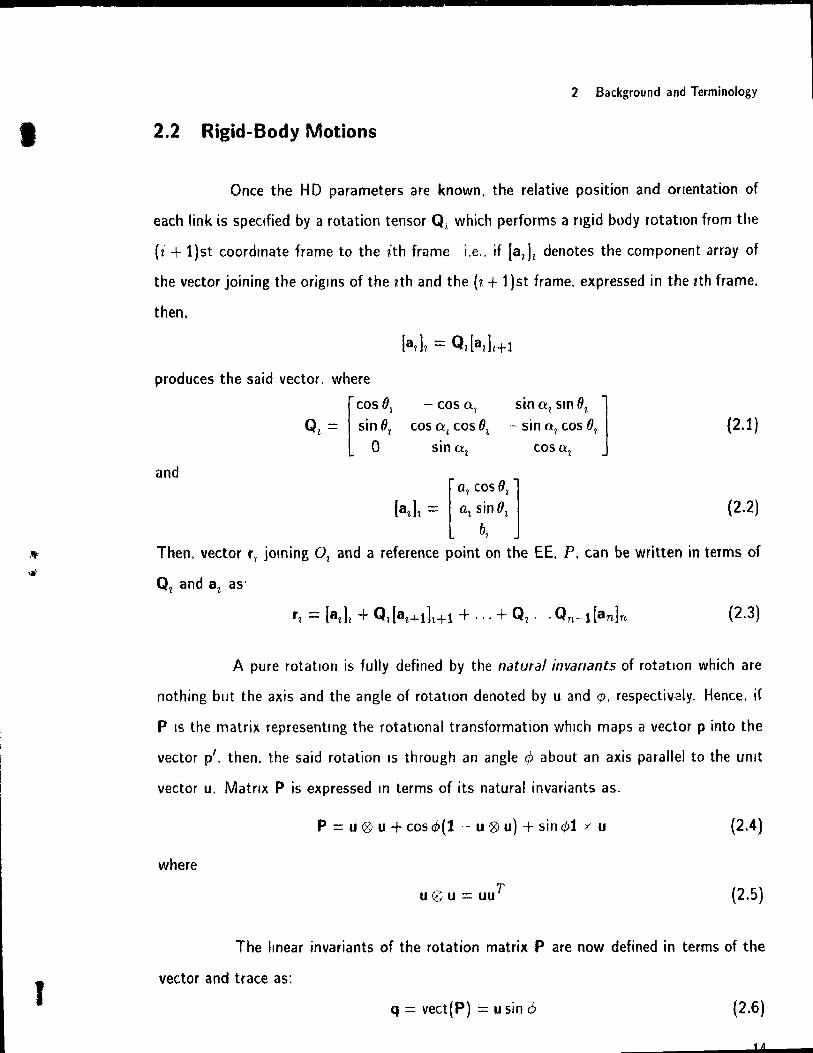
Once the H D parameters are known. the relative position and orientation of
each link is speclfied by a rotation tensor QI which performs a ngid body rotation from the
(i + 1 )st coordmate frame to the ith frame i.e .. if [al L denotes the component array of
the vector joining the origlns of the zth and the (z + 1 )st frame. expressed in the zth frame.
then.
produces the sa id vector. where
[
COS 81
Q! = si~Ol
and
- COS 0.1
cos al cos 01
SinD!
sin lXl Sin 01 ]
- sin 0:1 cos 8t
cos 0t
[
a? cos 01 ]
[a t ]1 = at s~~ 8t
(2.1)
(2.2)
Then. vector r1 joming 01 and a reference point on the EE. P. can be written in terms of
(2.3)
A pure rotation is fuHy defined by the natural invanants of rotation which are
nothing but the axis and the angle of rotation denoted by u and <p. respectiv~ly. Hence. if
P IS the matrix representmg the rotatlonal transformation whlch maps a vector pinto the
vector p'. then. the said rotation 15 through an angle cP about an axis parallel to the Unit
vector u. Matrlx P is expressed ln terms of its natural invariants as.
p = u tg! u + cos dJ(t - u Zi u) + sin cPt y u (2.4)
where
U 0 u = uuT (2.5)
The Imear invariants of the rotation matrix Pare now defined in terms of the
vector and trace as:
q = vect(P) = u sin dl (2.6)
14

t
,
2 Background and Terminology
and
90 = [tr(P) - 1)/2 = cos cp (2.7)
where
1 [P32 - P23] (2.8) vect(P) ="2 PB -- P31
Pl1 - Pl2
and
tr(P) = Pu + P22 + P33 (2.9)
Pz)" for t. J = 1. 2. 3 being the 1j element of matrix P. Also. vector and trace of a matrix
obey the relation
Ilvect(P)12 + [tr(P) -- 1)1/4 = 1 (2.10)
Another set of invariants which define a rotation are the quadratic invariant or
Euler parameters given as:
q' = sin (~)u (2.11)
The relationship between the linear and quadratic invariants can then be given as:
1 /1 + qo qo = ±\ -2-' (2.12)
2.3 Kinematic Closure Equations
ln thls thesis. the method adopted for formulating the kinematic closure equa
tions is as outlined by Angeles (1985). where the prescribed position and orientation of the
EE are equated to those produced by the manipulators Joint variables. The resultmg three
position equations and four onentation equatlons are denved from the Invariants of the EE
rotation matnx Thus, the 7 -dimenslonal vector of the kmematlc equations is defined and
the kinematlc closure equations formulated as:
[
2vect(Ql ' .. Qn) - 2u sin 4>] Il8) - x = tr(Q1' .. Qn) - 1 - 2 cos 4> = 0
l:ï[a?h - r (2.13)
15

J
. '
J{
2 Background and Terminology
where. r is the vector joinmg the origin of the fixed reference frame and the point P on
the EE. Moreover. Q1 .. ' Qrl specifies the rotation of the EE with respect to the fixed
frame which is assumed to be the one flxed to the robot base. For six-axIs manipulators
eq.(2.13) represents an overdetermmed system of equatlons but recalling eq.(2.10). it 15
obvious that the overdetermmancy is only formai smce only SIX equations out of the seven
are independent.
On the other hand. for spatial posing redundant manipulators eq.(2.13) repre
sents an underdetermtned system of m independent equatlons in n joint angles. Funher.
the Jacobian. J. of the aforementioned system of kinematic dosure equations is related to
the velocity Jacobian. K (Whitney 1972) as
J = HK (2.14 )
where
H = [1~:~(~~ ~f] 03 13
(2.15)
with 03 and 13 deftned as the 3 x 3 zero and identity matrices. respectively. 07' being the
three-dimensional zero vector. while K is given in the following form:
(2.16)
vector e1 bemg the unit vector parallel to the aXIs of rotation of the 1th joint.
The reader may come across certain repetltlons in the text. but. this has been
done in order to preserve the continuity .
16
1
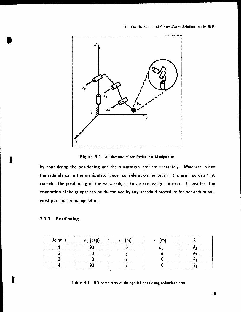
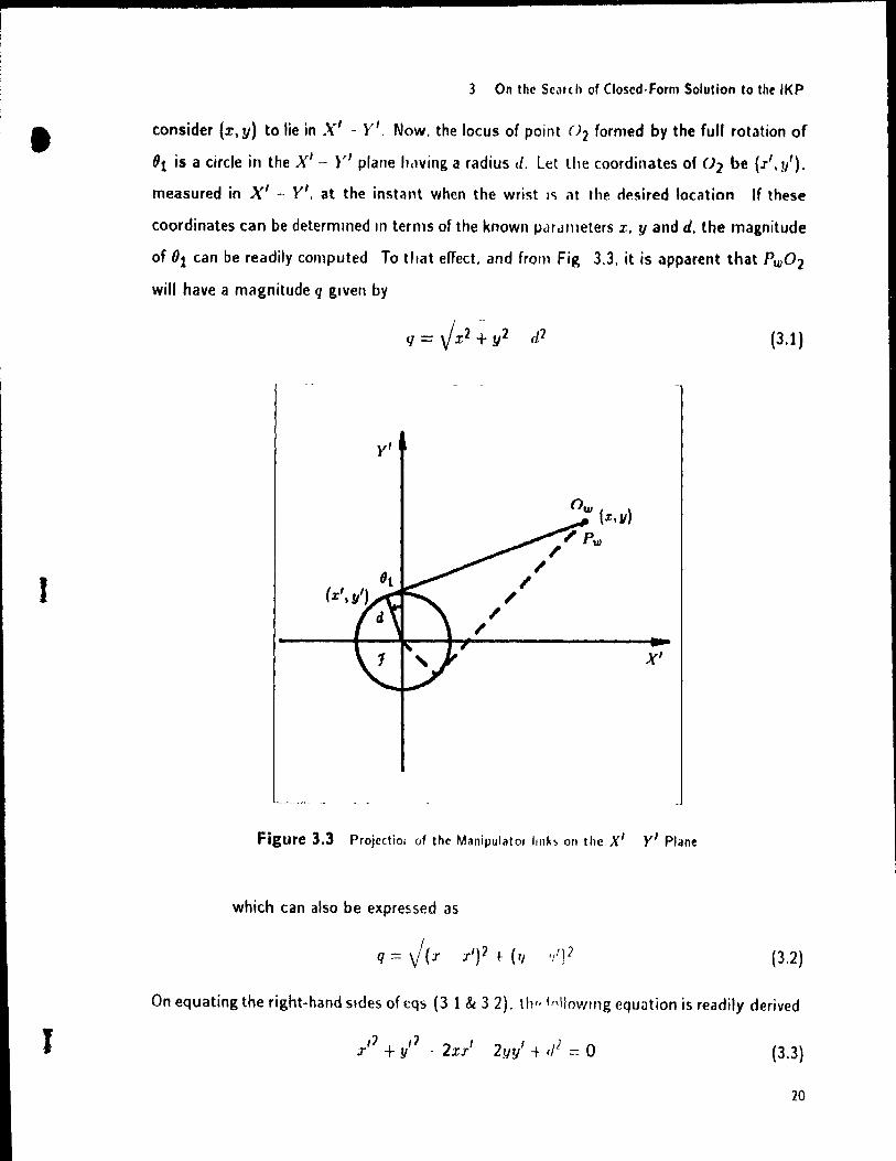
Chapter 3 On the Search of Closed-Form Solution to the IKP.
ln thls chapter we investlgate if closed-form Inverse kinematic solutions are
possible for a revolute coupled. redundant manipulator wlth simple. orthogonal. wrist
partitioned architecture while an objective function of the jOint angles is minimized. A
manipulator is said to be orthogonal if ail its consecutive jomt axes are oriented at angles
that are multiples of 7f /2. with respect to each other A wrist-partitioned architecture is
understood. In turn. as one ln which the tirst four joints form a subchain known as the arm.
the last three formmg the sphencal wrist Moreover. the Wrlst is termed spherical because
its three axes are concurrent Thus. the redundancy IS assumed only in the arm A majority
of the commefCIally available non-redundant manlpulators are of the wrist-partitioned type.
which allows a separation of the posltloning problem from the orientation problem.
The redundant mampulator for whlch the kmematic analysis is performed ln
this chapter 15 assumed to be derived From the non-redundant PUMA geometry. i.e .. an
addition al revolute joint is fixed to the shoulder. The first joint aXIs is oriented in the
direction perpendicular to the horizontal plane. while the three subsequent JOint axes of the
arm are paraI/el to one another and perpendlcular to the tlrst axis. Also. the tirst and the
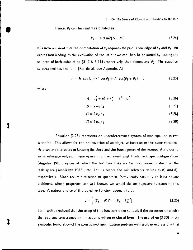
second axes are offset by a distance dm. as shown in Fig. 3.1.
3.1 Inverse kinematics
The inverse kinematics problem for a wrist-partitioned manipulator can be solved
,
1
1
3 On the S(';lI( h of Closcd·Fotnt Solution to thl! IKP
.,---_._----- -- - --------
z
x '----------
Figure 3.1 Arr~itectllre of the Redlllldi1llt Manipulator
by considering the positioning and the orientation problem separately. Moreover. smce
the redundancy in the manipulator !lnder consideratio:1 lies only in the arm. we can first
consider the positioning of the wn '.t subject to an optlmality criterion. Thereafter. the
orientation of the gripper can be detrrmined by any standard procedure for non-redundant.
wrist-partitioned manipulators.
3.1.1 Positioning
Joint t a1 (deg) (lI (m) --------- --- - -- -- --
1 90 o -2 -- -----3 4 ---
-0-- --- ---, - --0 -- --t
------ - -1 ---90 1
J
Il, (m)
?l cl o o
Ot - ~ ---~~ -. ____ }l. ___ _
°2 ___ _ ____ }l __ .
o ______ A_
Table 3.1 HO param.'tcrs of the spatial positiolllnr, rcdundant arm
18
3. On the Scarch of Closed-Form Solution to the IKP
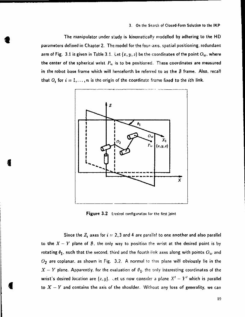
The manipulator under s~udy is kinematically modelled by adhering to the H D
parameters defined in Chapter 2. The model for the four-axIs. spatial positioning. redundant
arm of Fig. 3.1 is given in Table 3.1. Let (x, y, z) be the coordinates ofthe point Ow. where
the center of the spherical wrist Pu is to be positioned. These coordinates are measured
in the robot base frame which will henceforth be referred to as the B frame. Also. recall
that 0, for i = 1, ... ,n is the origin of the coordinate frame fixed to the ith link.
~------------~-------------------------~
1 1 1 1 1 1
• , 1 , l ...
z
...... .......
Figure 3.2 I,Icsired configuration for the first joint
x
Since the Z, axes for i ::: 2,3 and 4 are pamllel to one another and also parallel
ta the X - Y plane of 8. the only way to position the wrist at the desired point is by
rotating 61. such that the second. third and the fourth link axes along with points Ow and
02 are coplanar. as shown in Fig. 3.2. A normal te thls plane will obviously lie in the
X - Y plane. Apparently. for the evaluation of 81' the only interesting coordinates of the
wrist's desired location are (x,y) . . _et us now conslder a plane X' - y' which is parallel
to X - Y and contains the axis of the shoulder. Without any 1055 of generality. we can
19
,
1
1
3 On the SCJlth of CI05cd-Forrn Solution to the IKP
consider (x, y) to lie in X' - r'. Now. the locus of point ()2 formed by the full rotation of
61 is a circle in the X' - )" plane h,lVing a radius d. Let the coardinates of U2 be (r', y').
measured in X' - yi. at the instant when the wrist 1<; at the desired location If these
(oordinates can be determmed ln terms of the known par,lIneters x. y and d. the magnitude
of 61 can be readily computed To tltat effect. and from Fig 3.3. it is apparent that Pw0 2
will have a magnitude q glven by
(3.1 )
y'
X'
Figure 3.3 Projcctiol of the Manipulator link~ on the X' yI Plane
which can also be expressed as
(3.2)
On equating the right-hand sldes of cqs (3 1 & 3 2). th" f"llowtng equation is readily derived
,2 + ,2 , :r y - 2XI 2.11Y' + ,;1 = 0 (3.3)
20
c
c
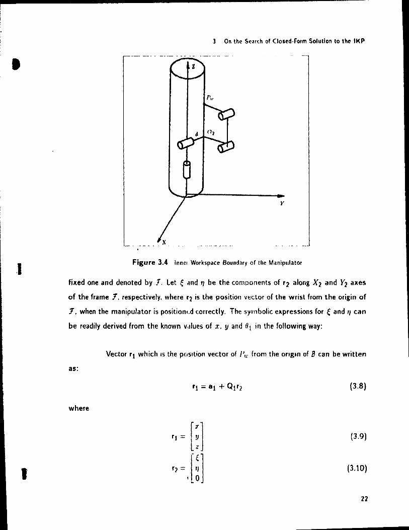
3. On the Search of Closed-Form Solution to the IKP
Since O2 lies on the circle of radius d. the following relation is valid.
,2 +,2 d2 x y = (3.4)
On substituti,ng the value of X,2 + yl2 from eq.(3.4} into eq.(3.3). the following expression
for x' can be derived. , d2 - y/y x=--
x (3.5)
When Xf is substituted from eq.(3.5) into eq.(3.4). a quadratic equation in y' is obtained.
as shown next.
(3.6)
The value of Xf can then be computed from eq.(3.5). If x = O. then eq.(3.5) need not be
considered and :r' is assigned a value of O. Equations (3.5 & 3.6) give the location of ()2
in the X' - y' frame. (Iearly. as long as (x, y, z) lies inside the manipulator workspace.
there will be two real solutions to the aforementloned quadratic equation. These solutions
will be identical if and only if the wrist is to be posed at a POint on the surface of the
cyltnder which forms the mner boundary of the workspace. as shown in Fig. 3.4. Imaginary
solutions will exist if. and only if. the wnst is requned ta Ile wlthin thls cylinder. which is
physically unattamable by a manlpulator of such an architecture
The angle. 01' by which the tirst Joint retates to position the wrist center at
the reqUired locatIOn ln space IS then calculated a5 follows:
{ arctan(i) - zr: , fit = x' 2 arctan(~),
if d ,t 0:
if d = O. (3,7)
As can be noticed. the manipulator joint-trajectory will have two branches correspondtng
ta each pair of values of x' and y'.
The next step is to determine an expression for ()2' To that effect. it IS con
venient to relocate our fixed reference frame Once (Jt has been computed. the remainrng
problem is reduced to performing the inverse kinematics of a planar three-link. revolute
coupled redundant manipulator, Now. the second coordinate frame IS assumed to be the
21
1
,1
1
3 On the Se3tC.h of Closed·Form Solution to tht IKP
y
Figure 3.4 Innci Workspace Boundary of the Manipulator
fixed one and denoted by " Let e ilnd 1] be the COnlPonents of '2 along X 2 and Y2 axes
of the frame ,. respectively. where '2 is the position vector of the wrist from the origin of
7. when the manipulator is positionc.d correctly, The s:fl11bolic expressions for e and '1 can
be readily derived from the known v.llues of x. y and 01 in the following way:
Vector '1 which 15 the pc/sltion vector of Fu: from the onglO of B can be written
as:
(3,8)
where
(3.9)
(3.10)
22
(
3 On the Searth of Closed-Form Solution to the IKP.
On deriving '2 as.
we obtain:
81 = [!] [
COS 01 0 sin 81 ]
Ql = SinOOl 0 - cos 81 1 0
~ = x cos 01 + Y sin {Il
Tl = z - bl
(3.11)
(3.12)
(3.13)
(3.14)
(3.15)
where bl is the length of the first link as specified in the Hartenberg-Denavit parameters
of Table 3.1.
Next. the following expression for r2 also holds:
(3.16)
Where at and 01 are defined in Chapter 2. The above equation. after a few lligebraic
and trigonometric manipulatIons. gives the following expressions. (See Appendix A for tne
complete derivations):
Where
and
N,_ = K 117 - K 2 e + 17 a3 cos 03 - ç a3 sin 03 + a21J
Ne = K 1 e + K 2 Tl + a3 e cos 03 + a3 ." sin 93 + a2 ç
D = .,,2 + ç-2
KI = a4 COS(03 + (}4)
K 2 = a4 sin(63 + (}4)
(3.17)
(3.18)
(3.19)
(3.20)
(3.21 )
(3.22)
(3.23)
23
t
3 On the Search of Closed-Forrn Solution to thr IKP
Hence. fh can be readily calculated as
O2 = arctan2 (.'\'._, Nf') (3.24)
It is now apparent that the computation of fJ] reqUires the pnor knowledge of (Il .md ()4 An
expression leadlng to the evaluation of the latter two can then be obtamed by addmg the
squares of both sldes of eq (3 17 &. 3 18) respectlvely. thus ehmmatmg 0] The equatlon
so obtained has the form (For detalls see Appendlx A)
(3.25)
where
'} 2 '} A = (14 + a3 + (J'} f.2 r/ (3.26)
8= 2a 3(14 (3.27)
C= 2U 2(13 (328)
D = 2 U4 (1] (3.29)
Equation (3.25) represents an ullderdetermmed system of one equatlon ln two
vanables. This allows for the optimlzation of an objective functlon ln the sanie variables
Here we are mterested ln keepmg the thlrd and the fourth Jomts of the manlpulator clo!'!e to
some reference values. These values mlght represent Jomt Imllt~. IsotroplC configuration.;;
(Angeles 1988). values at whlCh the last two Imks are far from some ob.;;tade m the
task space (Yoshikawa 1983). etc Let us denote the sa id reference values as Oj and °4,
respectively. Since the mmlmlzatlon of quadratlc forms leads naturally to Icast square
problems. whose propertles are weil known. we wou Id IIke an objective functlOn of thls
type. A natural choice of the objective functlon appears to be
(3.30)
but It will be reahzed that the usage of thls functlon 15 not suitable if the intention 15 to solve
the resultmg constrained minlmizatlon problem ln closed form The use of eq (3 30) ln the
symbolic formulation of the constramed mmÎmizatlon problem will result m expresSions that
74
1
1
t
3 On the Search of Closed-Form Solution to the IKP
are nonlinear not only in (h and (J4. but also in the sines and cosines of these joint angles.
This mixture of tngonometric functions of the joint angles and the angles themselves will
negate any possiblhty of obtaining a solution for ()3 and ()4 in closed form Hence. we choose
an objective function contalOmg only the sm es and cosmes of (}3 and (}4 Consequently.
the following objective function. which produces the same effect as that of eq.(3.30). is
selected.
z = ~[(sm03 - sin (3)2 + (cos 93 - COS(3)2 + (sin()4 - sin(4)2 + (cos 04 - cosO.;fl
(3.31)
Now. what we have at hand is a constrained minimization problem where the
constralOt equatlOn IS given ln eq.(3 25). Henceforth. for the sake of c.onvenience we
denote sin 93. cos 93. sin (}4. cos 04. sin (0 3 + (}4). cos (0 3 + (}4)' and the sines and cosines
of 0; and 84 as S3,C3.S4,C4,S34,CJ4,s3,,,,4,c; and c,4 respectlvely Thus. the constrained
minimizatlon problem in its entirety can be stated as
subject to
where
mmz x
(3.32)
(3.33)
(3.34)
The foregomg optimlzation problem is solved next by the classical method of Lagrange
multiphers. whlch involves the formation of an augmented function ç. The said function IS
formed by adjommg the constramt to the objective function via a Lagrange multiplier ..\. as
given next.
(3.35)
On the application of the first-order normality condition to the augmented func
tion. the following vector equation is obtained
(3.36)
25
a 3 On the Search of Closed-Form SolutlOll to the II<P
where the gradient is determined with respect to x. and J is the 1 . 2 Jacoblan matnx
formed by eva/uatlng the partial denvatives of the augmcnted functlOn wlth re~pe(t lo () 1
and 04 Hence. in terms of the sines and cosmes of {}J and "4. the Jacobliln ilnd the gradient
of the objective functlon are glven as
\'.:: = [(''>J ( '''4
(3.37)
(3 38)
Thus. eq (3.36) represents an overdetermmed system of two equations in one unknown.
namely À. Hence. in genera/ no À eXlsts whlch will verlfy eq.(3 36) exact/y. I.C wlth ICfO
error An error vector Co appears then. and a vector Ào that approximates the crror vector
wlth minimum Euclldean norm can be found Thus.
(3.39)
the solution vector Ào bemg
(3.40)
where (JJT) 1J is nothmg but the generalized mverse of J. What the normahty c..ondltlon
(3.36) states. then. IS that. al a statlonary pomt. the least-squcHe error. co. vanlshe!-J
On symbollc ellmlnatlOn of Ào. usmg eqs (3 36. 3 39 & 3 40). the followmg ').,t
of equatlOns IS obtained
where
and
1:'1 1(°3,°4) Y(()3' 04) = 0
11'2 h(()3,04)9(()3.04) =- 0
J(03· 04) = lJ(q"4 + '''3('4) + /J"4
h(03· 04) = /)(('3'''4 + bJ('4) + ('~3
/) cj '''4 q '~3
/) ('4 "'4 q '~3
(f •
~ .';4 q '''3
/) ('3 ('4 .~~
(3 41 )
(342)
(343)
(3.44)
(3.45)
16
1
3 On the Search of Closed-Form Solution to the IKP
Thus. the only conditions that will satisfy eqs.(3 41 &. 342) are that. either
(3.46)
or
(3.47)
Further. it can be seen that eqs.(341 & 3.42) are not dependent upon the Carteslan
coordinates of the desired location of the center point of the wrist. Hence. It becomes
imperative to consider the constraint equation (3 33) along wlth eqs.(3.41 & 342). to
obtam meanlngful results If the condition given in eq.(3.46) is satisfied. then. the following
relation between S3 and $4 IS obtained.
(3.48)
where
r = a4 (3.49) a2
Note that eq.(3 48) is devoid of the preassigned reference values 5j, cj, 54 and c4. Hence.
any roots obtalned by substltuting the sa Id equatlon Into eq.(3.33) will be spurious because
these equations do not lead to the mlnlmlzlng of the objective functlon Thus. the remaining
condition glven ln eq (3.47). along wlth the constraIOt equation. can be used to compute the
third and the fourth jOlOt angles A major consideration ln any numencal algonthm is the
conditIOn mg of th(l system of equatlons involved It IS observed that normahty conditIOns
are usually III condltlOned (Forsythe and Moler 1967). whlch is a major drawback. for
they can lead to kmematlc IOaccuracles. Wlth thls negatlve aspect ln mmd. It IS not
advisable to solve eqs.(3.33 & 347) numencally to obtain the values of the joint angles.
An efficient method of solvIOg the inverse kmematlc problem under study is by obtaming
the first two JOint angles of the arm m closed form using the expressions glven ln eqs (37
& 3.24). The constramed minimization problem of eqs (332-3 34) can then be solved uSlng
the computationally efficient orthogonal-decomposltlon algortthm (Angeles and Anderson
1987; Angeles and Maou 1988). as shown ln the example glven later. For the purpose of
numerical computation. the objective function given ln eq (3 30) can be used.
27
1
1
3 On thc Scareh of Closl'd ~orrn Solullon to Ihl' U<P
However, a question that cornes to one's mind is. how many root!. doe!'. the
system of equations (3 33 & 3,47) admit? To answer tlw, query. tlw ",)I(I !\y!>tt'm of
equatlon has to be expressed in polynomial form T 0 that eflect. let U!it 1/11 roduce th('
followlng half-tangent identlties
~ -'~I - C = 1
1 ,2 1
1 + t2 ' 1
((JI '1 = tan 2)' for 1 - 3,4 (J.50)
On substituting Il for Cl and .~,. for 1 = 3 and 4. In eqs.(3 33 & 347). the fol
lowlng equatlons are obtained, whlch can be vlewed as c!ther nonllncar algebraic equtltlon<,
ln t 3 and t 4. or trigonometflc expressions in the two JOint angles {}J and 04 The dertvatlon~
that follow were performed with computer algebra us mg MACS Y MA. ThiS produced
(;4t~ + C]'~ + C2f~ -t Cl'3 + Co =:. 0 (3.51 )
where
C 4 =Qtl+tl+ V/ 4 (3.52)
C] = Kt: + (Ttl -+ lV/4 + () (3 53)
C2 = U~ + PI~ -t X '4 l, (3.54)
Cl = M'~ + .\'I~ -t /('~-t l' '} r '4-t '4-t 1 (3.55)
(' '''i/ 3 /0 =. 4 Tf~+~f4 (3.56)
and
K = 2 (,' '''4 2 IJ .~ 4 + 2 /) .0; i (3.57)
L = 4 IJ ('3 (3 58)
AJ = 2 (; '''4 2 [) '''4 2[) '''3 (3.59)
N = 4 (,' r4 4 /) r4 4/1 rj + 4 IJe; (3.60)
p= 4 [) ... ; (3.61 )
Q= 2 [) '''4 2 /1 .~ j -t 2 [) ." 3 (3.62)
78

1
f
also
where
3 On the Search of Closed-Form Solution ta the IKP
R =: -4 D c4 -- 4 B cj - 4 D c3 + 4 Ccl
S =: 2 D 84 + 2 B s3 + 2 D '<;3
T =: -4Dc4
U=:4D84 ~. =: 2 D b 4 -- 2 B "3 + 2 D 83
li' = 4 D c3 + 4 C c4 + 4LJ c,4 - 4 B ('3 X=-4[)$3
y = 4 C c4 + 4 [) {'4 - 4 B c3 - 4 D ci z = - 2 D '''4 + 2 B s3 + 2 D 83 o =: -2e 84 - 2Ds4 - 2D"'3
1 = - 2 C 84 -- 2 D 84 + 2 D 83
E=A+B-C-D
F=A-B+C--D
G=A--B-C+D
li = --4D
J=A+B+C+D
(3.63)
(3.64)
(3.65)
(3.66)
(3.67)
(3.68)
(3.69)
(3.70)
(3.71 )
(3.72)
(3.73 )
(3.74)
(3.75)
(3.76)
(3.77)
lJ·78}
(3 /9)
variables A, B. C. D bemg dehned ln eqs.(3.26-3 29) Equation (3.74). which is quadratlc
in t3 can now be solved for the same. th us giving the foliowlOg symbolic expression:
-H t4 = \/H2 là - 4(E + Gt~) (Ft~ + J) t3 = ---- - - (3.80)
2(E + Gtn
On substituting the values of t3 from eq.(3.80) into eq.(3.51). a 24th order
polynomial ln t4 is obtained as follows: 24
LA, t4 = 0 (3.81) 1-==0
29

1
,1
t
) On IIH' Sf'OIrch of Closed·Form Solution 10 tht' IKP
thus signifying that the system of equations (333 II 3.47) will have 24 roots. Here At are
the coefficients of the polynomial giv~n in Append/x 8. The computatIon of the roots of th.s
large polynomial is very inefficient because of thr "in' of the coefficients and the number
of computatIons mvolved ln cornputmg them. Moreover. even a reasonable value of t4 wIll
acquire a large magnitude when ra/sed to the power of 24 For example. at (J4 ::: 3rr /4
t4 = 2.4142. but t4 24 acquires a magnitude 1.5368 ' 109. Such hlgh magnitudes are
undesirable from the pOint of vicw of round-off errors. Of academic interest is the fact
that the roots of the polynomial wi~1 represenl dl! lhe statlonary points of the dugmented
funetion in eq.{3.35). Thus. the solution to the constrained minim.zation problem will be
twice the inverse tangent function of the root. Iying dose st to 84,
2
OrlllR 01 Robot
v
., _._-, ------'
Figure 3.5 Cartesiall trajfctory
It is therefore obvious th;:lt even a simple> redundant arm architecture does not
allow for an explicit closed-form kinematic inversion. ,ft'hlle mmimiling a performance index.
Another aspect brought out by th/s digonthm wh/ch I~ mteresting From purely a theoretical
viewpoint is that. the inverse kinematic problem under study leads to a 2-dimensional
30

3 On the Search of Closed-Form Solution to the IKP
optimization problem. which is relatively simple to handle. The closed-form solution of a
spherical wrist being common knowledge, 1 will not dwell on it in thls thesis.
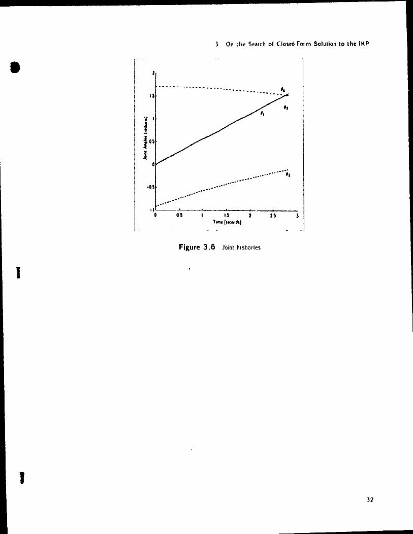
3.2 Example
ln this example. the spherical wrist of the redundant manipulator is required
to trace a hehcoldal traJectory. The robot is assumed to be stationed at the ongm of the
frame in which the traJectory is defined. as shown in Fig. 3 5. The trajectory parameters
are as given below'
x = a cosB
y = a sin fi
z=b{3+2
where a = 1.5, b = 3/'ir, 0 S f3 :s 1r/2. f3 being the angle between the X-axis of the
robot base frame and the projection on the X - }' plane. of the position vedor of the
point on the trajectory where the wnst IS to be positloned. The dimensions of the first.
second. third and the fourth links are taken as 2.m. 2m. v'2m and lm respectlvely. The
ratios of the lengths of the second. thlrd and the fourth Irnks correspond to those of
dextrous fingers (Salisbury and Craig 1982) The offset at the shoulder was considered
zero. Additlonally. the values of 03 and 04 are specifled as 94.08 - and 97.4r. respectively.
This would result ln the second. thlrd and the fourth links attarnlng isotropie confIgurations
(Angeles 1988). Jornt angles 03 and 04 are determined by solving a constrained mmimlzatlon
problem where eq.(3.25) glves the constralnt and eq.(3 30) represents the objective functio.l
to be mlnlmlzed The solution to the aforementloned constrained mlnlmization problem
was obtained usmg QUADMIN software package (Angeles and Maou 1988: Anderson and
Angeles 1987) The reference values of the two variables were supplred as the sensible
Initial gU€GS to the Îteratlve subroutine. in which case it took less than four iterations
before convergence to the exaet solution was obtained. The error norm was specified as
1 x 10--8. The resulting time histones for the first. second. thlrd and the fourth joints are
deplcted ln Fig 3.6.
31
3 011 the Semh of Clostd rOtin Solution to tht IKP
---_ ................ ... .... .. .. .. .... .. .. .. . .. .. .. .. .. .. .. . 15
'f
·u
.......... ... ft!".<#J " ..........
.. -.", .. 000
.00 00·
"'."' ..... ", ...
• 0
" .... ·I~--~~--~----~--.... ~----~----o 05 I,~ 2
T,m. (second.)
Figure 3.6 Joint hIstories
1
1 32
Chapter 4 A Resolved-Rate Control Aigorithm
4.1 Introduction
As is evident from the literature survey, one of the major drawbacks of the
schemes proposed for the solution of the inverse kinematics of redundant manipulators at
the joint-rate levells that they lead invariably to noncydic trajectories. With the formulation
presented in this chapter, linear equations in the joint rates lead to cyclic trajectories.
The said system of Ilnear equatlons is formed by differentlatmg the flrst-order normahty
conditions-of the assoclated nonlinear mathematical-programmmg problem-with respect
ta tlme. whlch are then adJorned ta the differentlal relation between the joint rates and the
(arteslan velocltles
For solving the Ilnear system of equatlons. two different approaches have been
employed. In the first approach. it has been shawn that. under certain conditions that are
usually met. the jomt rates can be determined by solvmg a linear constrained minimization
problem involving the mimmizatlon of the welghted joint velocitles. In the absence of
those conditions. the said jOint rates are computed uSlng LU decompositlon. The linear
constramts are the differentlal relatIons between the joint rates and the Cartesian velocities.
ln the second approach. the fjrst-order normallty condition is expressed in terms
of the veloclty Jacoblan and a modified Lagrange-multiplier vector which IS an implicit
function of the jOint variables. Simllarly. the difTerentlal relation between joint velocities
1
..
" A Rcsolv('d Ratt' (ont roi AIRon1 hm
and Cartesian veloclties. used in the first method. IS repl.lced by tht> dlnerenllal ft'Iallon
between the Joint rates and the end-eflector tWist The resultmg ~yst('Fn of equ •• tlon ...
is solved simuitaneously to glve the Jomt rates and the ratc!:. of change of 'hE' mo(fIf,ed
Lagrange-multiplier vector
Three examples are salved to Illustra te the fact that thl~ scheme ellflllnate~ the
non-conservat.ve effects
4.2 Resolved-Rate Schemes for the Kinematic Inversion of
Redundant Manipulators
First. the variables that will be used extenslvely throughout this chapter are
defined.
The number of axes of the manlpulator will be denoted by 1/. the dimenSIOn of
the task space bemg m. For example. ni =- 2 in case of a planar positlomng task. ?n =- 3
for the case where the end efTector IS to be posltlOned ln the 3· dmlcnslonal Carteslan space:
and ni = 6 for the problem of posltlonmg and orientlllg the EE ln the 3-dmlenslonal space
It will be assumed that m < n. Furthermore. fi kmcmJtlc con~tramt equations are prcsent.
out of whlCh only 7n (m <'. p) equatlons may be Independent
The kinematlC constramts can be represented .,yrnbolltally as
g(O) = x (4.1 )
where x is the m-dlmenslonal vector of Cartesian coordlO,ate~ and g IS the p-dlmenslonal
vector of kmematlc constramt equatlons
Kmematlcally. equatlon (4 1) represent~ the po~,tlonlng and Orientation reqlJlre
ments of the task at hand Aigebraically It represents an underdeterrnmed system of tri
mdependent equatlOns ln n unknowns From a computatlonal pomt of vlew. the kmematlc
constraints can be expressed ln terms of the rotatlonallflvanants and the position vectar of
34

t
4 A Resolved-Rate Control Aigorithm
the end effector as given in eq. (2.13). In the most general use of m = 6. this formulation
leads to a system of seven equations in n unknowns. out of which only six equations are
independent (Angeles 1985). The extra degrees of freedom in the manipulator architecture
allow for the optlmization of a performance mdex. which we deflne as the quadratic functlOn
z given below.
(4.2)
where. f 15 a nonlinear. q-dimensional vector functlon of () The choice of the performance
index is dependent on the nature of the task to be performed and any particular cntenon
to be satlsfied while performing the task. Thus. the problem ln its entlrety can be stated
as follows:
subject to
min z(O) o
g(O) = x
with W defined as a q > q symmetric, positive definite welght matrix.
(4.3)
Using the classical Lagrangian approach one can reformulate the foregoing con
strained mtnimlzation problem in the form of an unconstrained minimlzation problem. To
this end the augmented function ç. that IS to be minimized. is defmed as:
((0) = z + >.T(g -- x) ----. min N
(4.4)
subject to no further constraints. >. bemg the rn-dlmensional vector of Lagrange multlplters
From the first-order normality conditions. a stationary point is reached if the gradient of ,
with respect to () vanishes. Hence the followmg is obtamed:
(4.5)
where J denotes the m x n displacement Jacobian matrix. namely. the partial derivative of
g with respect to (). i e .
(4.6)
35
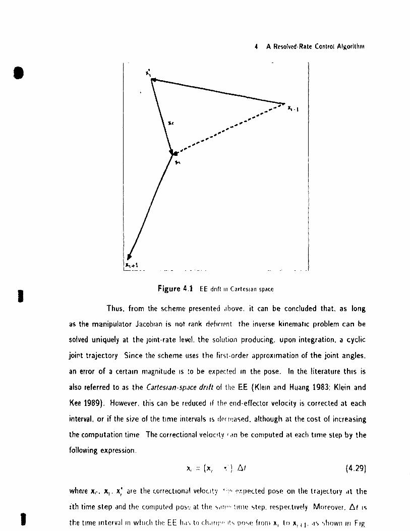
..
4 A Resolvcd R.lle (ontrol Aigorithm
The displacement Jacobian for the redundant formulation of the kinematlC constratnts is
of the followang form'
[
(ttrQ "Q)A] J = 2q 1 A
B with A. Band q defined as:
q = vect(Q)
(4.7)
(4.8)
(4.9)
(4.10)
where el is the Unit veetor parallel to the aXIs of rotation of the lth JOint and rI IS the vecter
directed from the origin of the 1th coordlnate frame to POint J) of the EE ln eq (4.5). A
can be thought of as a veetor that is mapped by JT onto \'z Thus. eq (4.5) represents
an overdetermlned system of ri, equatlons ln m unknowns. namely the", colllponents of A
Henee. In general. no veetor A exists which will verify eCl (4.5) exactly i.e. with zero error
An error veetor e(O) appears then. and a veeter. Ao. that approxlmates the errar veetor
with minimum Eueltdean norm can be found. Thus.
(4.11)
the said veeter ,1.0 betng.
14 12)
where (J T) 1 represents the Moore- Penrose generahzed tnverse of fI . drfmed as
(4.13)
What the normahty conditIon of eq (45) states IS that. at a statlOnary pOint. the least
square error e( 0) vamshes
Until now ail the computations were performed at the JOlnt-toordtnate level. but.
stnce our tntercst Iles in devising a resolved-rate control scheme. we can easlly formulate
the inverse kinematic problem at the jOint-rate level by d,fferent,attng eqs (4 1 & 4 5) with
respect to time. which th us ylelds
(4 14)
1
c
4 A Resolved-Rate Control Aigorithm
(4.15)
The usage of the joint rates in the determination of jT makes it unsuitable for application
in its present form. Thus. jT~ will be represented in a form that is linear in the joint rates.
To this effect. we defme a vector pas:
Then. in index notation. p can be represented in the following fashion:
dJ'2k Pl = -dt-À.k
where J~k is the (l.k) entry of JT. Smce J is a function of Oonly.
dJtk _ alt~iJ di - aOI 1
and hence.
where
(4.16)
(4.17)
(4.18)
(4.19)
(4.20)
thereby showing the lineanty dependence of p upon (J Here ~tl is the (i, 1) entry of a
matnx A whlch IS. thus. defined as:
(4.21)
Thus. In invariant form the followlng relation holds
(4.22)
Upon substitution of eq (4.22) lOto eq.(4.14). the latter can be written in the following
form
JT). + MO = 0 (4.23)
where M denotes " + V2 z Equations (4.23) and (4.15) can be rearranged to obtain a
system of equations that are linear in iJ and À.
(4.24)
37
1
4 A Rcsolvcd-Ratt' (ont roi Aigorithm
The matrix comprising the coefficients of the joint rates and the rates of change of the
Lagrange multipliers in eq (4 24) IS henceforth referred to as the coenlClefll m,llflA ,lI1d
denoted by R. We now have the following
Theorem 1 Dependmg on whether M is positive de/mite, lIegative deftlllte, or SIglI ",del
imte, R IS negatlve dehn/te, positive dehmte or sign ;n defi", te, respective/y.
Proof See Appendix C.
Further, eq (4.20) can be wntten in terms of the components of the kmematlc
constraints as.
k == 1. .. 7ft. (4.25)
or. in invariant form. a2(gT ,q
" = --ao2 (4.26)
where gk IS. obviously. the kth component of the vector g Equation (4 25) proves that "
IS a symmetric mat ri x which, together wlth the symmetry of the Hesslan of the objective
function. leads to the conclusion that M IS a symmetrlc matnx too However, eqs (4 14
& 4.15) do not guarantee a minimum of ;:;, because the second-order normallty conditIOns
are not enforced, but only expected to be satlsf,ed. By ftndtng the ~tarttng pOint on the
trajectory via a nonllnear constratned mtnlmlzatlon problem as deswbed ln (Angeles et al
1987, Angeles. Anderson 1989), the subsequent potnt~, computed by the Itnear scheme
presented ln thls chapter, the JOint configurations obta,ned at the5e pomts will produce
a mintmum From eqs.(4 15 & 423), a general solution for the JOint velocltles can be
obtained by ellmlnatmg ..\ from them. This takes on the forrn
(4.27)
Obviously. computing 0 dlrectly from the expression glven above IS not advisabie. for It
reqUires the IIlverSlon of matrices whlch, more often than not. tend to be .11 tondltloned
(Golub and Van Loan 1983) Next, a theoretlcal result is presented, that. under certain
1
f
4 A Resolved-Rate Control Aigorithm
conditions. allows the computation of the solution of eqs.(4.15 & 4.23) from a constrained
linear least-square problem.
Theorem 2: For points where M is positive definite. the solution è of eqs.(4.15 & 4.23)
is identicaJ to the solution of the following minimization problem'
subject to
JO = x (4.28)
Proof: See Appendix C
The solution to thls linear constrained mmimization problem can be efficiently
computed uSlng the orthogonal-decomposition algonthm. discussed elsewhere (Angeles et
al. 1987). The joint rates can then be integrated in time in order to produce the desired
joint-coordmate tlme histories.
ln Example 4.1 given later in this chapter. this procedure is used to track a
circular. planar traJectory If M 15 sign indefmite. then. obviously the Jomt velocities cannot
be computed USI'lg the Irnear constralned minimlzation formulation. eq.(4.28). Indeed.
whereas the nonllnear problem (4 3) a'ways admlts a minimum and. in facto this can be
computed usmg suitable methods for constramed nonlinear least-square problems-see. for
example. (Angeles et al 1987) and the references therem-, the unconstramed hneartzed
probJem of eq.(4 24) can be formulated as a mimmlzatlOn problem only if M is positive
deffnlte. However. nothmg ln the prevlous derlvatlon guarantees that M will be posItive
definite. In facto as shown ln Example 4.2. M can become sign indefinite. The reason
for this IS that problems (4.3) and (44) are equlvalent only up to flrst order ThiS means
that they both share the same statlOnary pOints. but these ",e not necessarily of the same
nature (See Appendix D). That is. if the statlonary point is a minimum of probJem (4 3).
it may be a saddle point of problem (44). NevertheJess. even if M is sign indeflnlte. the
joint rates can be computed usmg the LU decomposition (Golub and Van Loan 1983) of
matnx R in eq (4.24)
1
1
• IL,
4 A Resolvcd·Rate Control AllI.orithm
Figure 4,1 EE drift III CartcSlaI1 spacc
Thus. from the scheme presented ,lbove. it can be concluded that. as long
as the manipulator Jacoblan is not rank d<>fl(fpnt the inverse kinematlc problem can be
solved uniquely at the Joint-rate lev.cl. the solution producing. upon integration. a cyclic
joil't trajectory Since the scheme uses the first-order approximation of the joint angles.
an error of a certain magnitude IS to be expected ln the pose. In the literature thls is
also referred to as the Cartes/an-sfJr1Ce d,dt of the EE (Klein and Huang 1983: Klein and
Kee 1989). However. this can be reduced If the cnd-effector velocity is corrected at each
interval. or if the sile of the tlme Întervals IS drneilc;ed. although al the cost of increasing
the computation time The correctional veloclty (,ln be computed al each tlme slep by the
fo"owing expression.
x -- ( ~ ": ", 6 f 1 - 1 (4.29)
where X(. Xl' x; are the torrec.tlonal velouty 1 :1" ~·hpe(.led po~e 011 the lraJettory ,It the
ith time step ,md the c.omputrd po~'~ al the ':>d:1\" t!llle .,tep, respectlvely Mor('over, !:ll 1<;
the tlme IntcrvJlm w!1\ch the EE h,!') to (h,II'~'{' 1«, po'-.e frolll x, tn X, ~ l, ,1\ ..,howil I!I F IR
(
(
f
4 A Resolved-Rate Control Aigorithm
4.1.
Next. an alternative procedure is presented. that produces the sa me solution.
but is computationally more efficient to apply. As opposed to the previous procedure. this
one IS based on the velocity Jacobian K. which IS simpler to evaluate than J. The matnx
representation of the veloclty Jacobian IS glven in eq.(2.16)
Let t be the six-dimenslonal twist vector of the end effector. which is defined
as
(4.30)
where w Îs the angular velocity of the EE and j Îs the velocity of the point P of the EE. as
defined prevlously. Then. matrix K IS defined as that mapping () into t. i.e ..
K(} = t (4.31)
As shown in eq.(2.14). J and K are related by:
(4.32)
Now upon substitution of eq.(4.32) into eq.(4.5). the following relation can be derived.
(4.33)
where "''' is the six-dimensional modtFied Lagrange multiplier. defined as'
(4.34 )
Thus eq.(4.14) can be rewritten in terms of the velocity Jacobian as:
(4.35)
Equation (424) can th us be rnodlfied and reformulated in terms of the velocity Jacobian
and the EE twist. namely.
(4.36)
1
1
4 A Resolvcd·Rale Contlol Aigonthm
where. M* is defined as V2: + A· and A" I~ the following
A' ::: a (KT".) dO
(4 37)
The evaluation of A* reqUires the formation of il thlrd-r,mk tensor. which 15 "Iu~trat(ld
below. Note that A and é are the two miltm, components of K. 1 t~ .. if.
then. the third-rank tensor iJK / (JO can be repre~ented symbollcally as.
dK ::: [aA/aO] ao aB 1 dO
., .
(4.38)
(4.39)
Where. aA I ao and aB / (JO are. themselves. third-rank ten~ors and take on the forlll~
(Derivations of the said third-rank tensors arc mcluded in Appendix E.)
0 0 0 o o o
el ' e2 0 0 dA
- el . e3 e2 > e3 0 ao
(4.40)
et " eu el ' cri .. erl . en 0
and
el < (et· rt) el " le2 . r2) el (e3 ' r3) Ct ( Cu . r ri )
aB e] ! (e2 r2) el (e3 . r3) c, (eu . r TI) (4.41) -- --ao Sym
erl ' (cri . rtl )
ln order to have consistem.y ln the notation the rrldlnx coeffiCient 111 eq (4 36)
IS represented sYlllbollcally by R-. Analogous to eq (4.20). the (1./) component of A" Lan
be expressed ln the component forlll as:
_ df..· zh 4
A 'd::: (JO 1 À ~ (4.42)
Here. k1k is the (l.k) component of the transpose of the veloclty JIKoblan The sHnilaflty
between A and ,. ... however. ends at eq (442). SII1c.e ktk I~ not a Hes~lan matrlx. 1 e . no
scalar functlon eXlsts whose matnx of ~ec.ond derIVatlves be 1\" Ttll~. ot)VJou~ly, clrl~e!l
from the fact that. properly speaklng. K IS flot il Jacob'dn matflx. 1 e , no V('C.tor functlOn
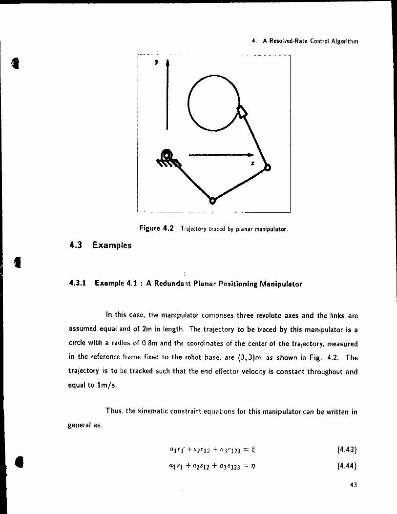
t
t
4. A Resol'led-Rate Control Aigorithm
Figure 4.2 l.-ajectory traccd by planar manipulator.
4.3 Examples
4.3.1 fxample 4.1 : A Redundu'll Planar Positioning Manipulator
ln this case. the manipulator compnses three revolute axes and the links are
assumed equal and of 2m in length. The trajectory to be traced by this manipulator is a
circle with a radius of a.8m and thf coordinates of the center of the trajectory. measured
in the reference frame fixed to the robot base. are (3,3)m. as shown in Fig. 4.2. The
trajectory Îs to be tracked su ch that the end effector velocity is constant throughout and
equal to tm/s.
general as.
Thus. the kinematic con~traint equatlons for this manipulator can be written in
al('l' + Q2ct2 + (]3''123 = ~
al s1 +a25 12 + a3 5 123 = q
(4.43)
(4.44)
43
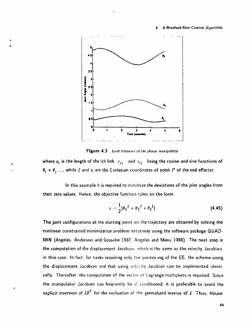
..
4 A Rt'solved·Rate Control A.ljl.orithm
o~--~----~--------~ _____ ~ __ ___ o 2 J • ,
T_I--"I
Figure 4.3 Joint histones of the planar manipulator
where al is the length of the ith linl<. rI) and .'11) being the cosine and sine functions of
0l + 61 .... while e and TI are the Cartesian coordinates of point P of the end efTector.
ln this example it is required to mininllZe the deviations of the joint angles from
their zero values. Hence. the objective functlOn takes on the form:
(4.45)
The joint configuratIons at the start mg pOint on the trajectory are obtained by solving the
nonlinear constrained minimization problem IterLltlvely using the software package QUAD
MIN (Angeles. Anderson and Gosscllll 1987. Angeles and Maou 1988). The next step is
the computation of the dlsplacement Jacoblùn. 'Nhlch is the same as the velocity Jacobian.
in this case. In fact. for tasks requiring only tlle posltioung of the EE. the scheme usmg
the displacement Jacoblan and that using v~lc~ Ity Jac.obian can be implemented identi
cally. Thereafter. the computation of the vectcr cf Lagrange multiphers is required. Smce
the manipulator Jacob,an can frequcntly be dl c.ollditloned. it is preferable to avoid the
explicit inverSion of JJ T for the ev,.!uation of ~ he generahzed inverse of J. Thus. House~
44
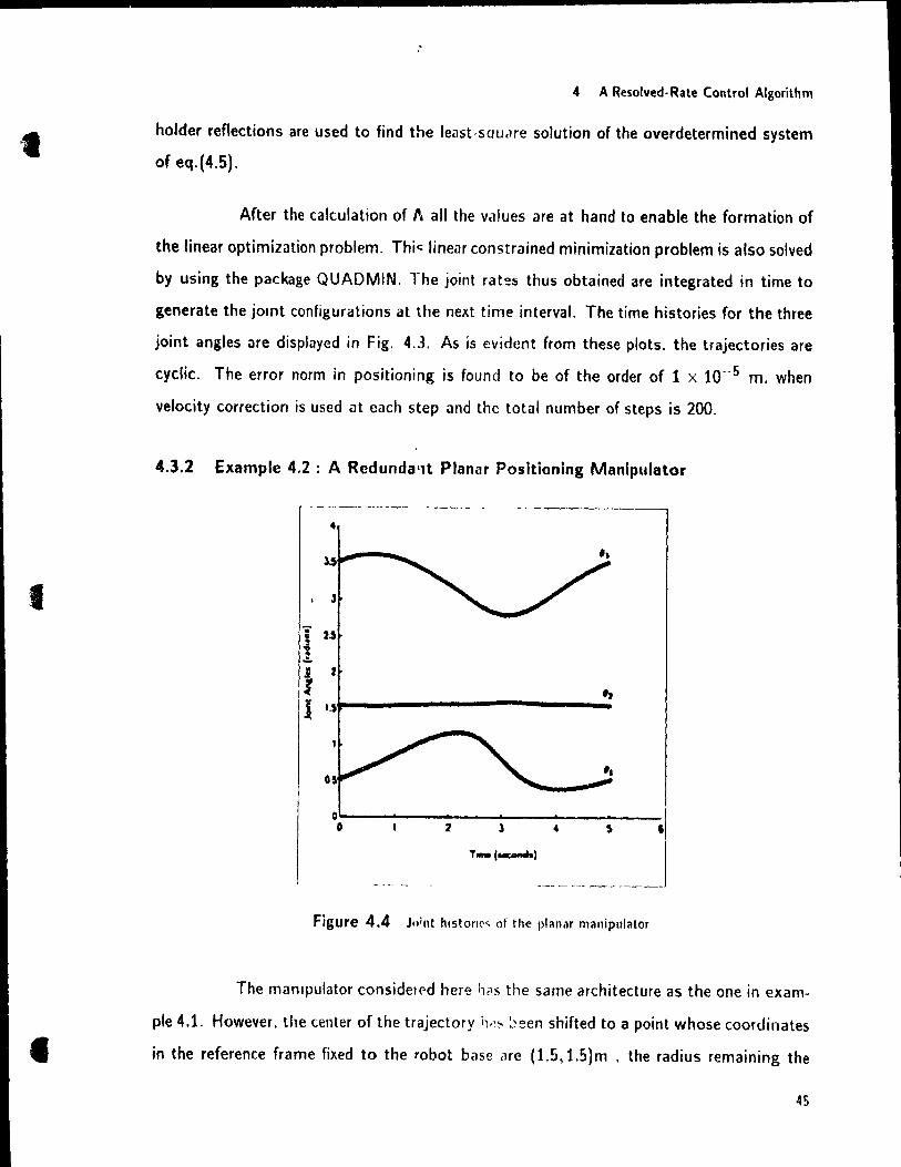
1
1
.. A Resolved-Rate Control Aigorithm
holder reflections are used to find the least-SQUcHe solution of the overdetermined system
of eq.(4.5).
After the calculation of l'. ail the values are at hand to enable the formation of
the linear optimization problem. Thi.; linear constrained minimization problem is also solved
by using the package QUADMIN. The joint rat~s thus obtained are integrated in time to
generate the jOint configurations at the next time interval. The time histories for the three
joint angles are displayed in Fig. 4.3. As is evident (rom these plots. the trajectories are
cyclic. The error norm in positioning is found to be of the arder of 1 x 10-- 5 m. when
velocity correction is used at cach step and the total number of steps is 200.
4.3.2 Example 4.2 : A Rcdunda'lt Planar Positioning Manlpulator
- - ------------,
•
, 3
;;;-U " -i ..
.::. J , 1 ë 1.$ ~
l,
O~--------------~----~ ____ ~ ____ I o ~ 3. ,
Figure 4.4 Joint hIstorie" of the planar manipulator
The manlpulator considelC'd here IlèS the same architecture as the one in exam
pie 4.1. However. the center of the trajectory ll.~~ ~een shifted to a point whose coordinates
in the reference frame fixed to the robot base élre (1.5,1.5)m . the radius remaining the
45
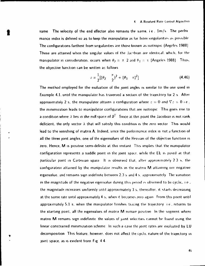
1
4 A Rcsolvtd Ratt' (onllol AIj1,ollthm
same The veloclty of the end efTector also remalns thE' 5ame. i e. 1 m /!. The perfor
mance mdex is defmed 50 as to keep the manrpulator as far tram !>lngularlt,{·" ,b po ...... ,blt·
The configurations farthest trom smgulantle!> are those known .1 ... I!>OtroplC (Ang('I('~ 1988)
These are attamed when the smgular values of thE' J,j(',t"lIan ar(' IdentK.ll. whl( h. for tlw
mantpulator ln consideration. o(turs when 0] = 7l 2 and 03 :~ r, (Angcle') 1988) Thu ....
the objective functlon can be wfltten as follows
(4.46)
The method cmployed for the evaluatlOn of the jomt angles 15 slmdar ta the one used III
Example 4.1. untll the manlpulator has traversed a section of the trajec'ory for 2 s Aftt'Y
approxlmately 2 s. the mampulator attams a configuratIOn where ::: :..: 0 and \' ,:: =- Ole.
the mmlmlzatlon leads to manipulator configurations that are Isotroplc This glvc ... nse to
a condition where À Iles ln the nuH space of J T Sirice at tOls pOint the Jacoblan 15 not r ank
deficient. the only vector À that will satlsfy thls conditIOn IS the zero vector ThiS would
lead to the vamshmg of matnx 1\. Indeed. Slnce the performance Index IS nol cl functlon of
ail the three jOint angles. one of the eigenvalues of the H('ssian of the objective functlon 15
zero, Hence. M 15 positIVe seml-definite at thlS Instant ThiS Imp"e~ that the manlpulator
configuration represents a saddle pOint m the JOint spaCf'. wh ,le the EE I~ pO'ied cH that
particular pomt ln Cartp-slan space It 15 observed lhat. after approxlfllJtf'ly 2 3 ~. Hw
configuratIOn attamed by the manipulator re ... ult!:> ln the mat flX M all.lHlHlg olle negatlve
elgenvalue, and TemalnS sign mdefllllte between 2.3 sand 4 ~. approxHllately The VJrlatlOn
ln the magnitude of the negatlve elgenvalue durmg th,s penod 's ob<,crved to be cyelte 1 (' •
the magnitude Increases unlformly untll approxlmately 3 <,. thereatter. Il .,tart':> dt'ereaslng
at the same rate untll approxlmately 4 s. when It bpcome"i zero agalll From thls pomt untll
approxlmately 5.1 s. when the manlpulator t,rllshes tr.ltlng Hw traJettory 1 e . returns to
the startmg pOint. ail the elgenvalues of matrlx M r~mall" pOSitive ln the segment where
matm: M remalns sign Indeflmte the values of )0111t veloutles cannot bf> found usmg the
hnear constramed mlnlmlzatlon scheme ln such a case the JOint rates ,Ir(' cvaltJcllcd by LU
decomposltlon ThiS feature. however. does not affect the (yellc nature of the trtljectory ln
JOll1t 5pace. as 15 eVldent trom Fig 44
46
1
1
1
4. A Resolved·Rate Control Aigorithm
Joint , 1 2 3 4 5 6 7
1 , 1 1 1 1 ,
, 1
'T7"'l0"J'rl,...,...... - - - - - '- - - - - - - .,J 1 , 1 /'" 1 ,~ , , ,~~ ...
Figure 4.5 CYBOTECH P·1S architecture.
a, (deg) a, (m) h, (m) 90 0 0.16
180 0.16 0 -90 0.2 0
90 0 0 90 0 0.14 90 0 0
-90 0 0
Table 4.1 HD parameters of CYBOTECH P·t5
4.3.3 Exemple 4.3 : Seven·Axis Path Tracinl Manipulator
..
IJ~
IJt 1J2 1J3 IJI. Br. 1J6 67
This example iIIustrates the usage of the velocity Jacobian. The trajectory to
be traced is circular and is assumed to be located on a plane having the equation:
x = d, for d = 0.16m
The manipulator chosen for performing the task is the redundant. wrist-partitioned ma-
47

1
l
l
4 A Resolved Rate Control Aigorithm
z
~----------------. y
x
Figure 4.6 ,rajcctory Ir.l(rd by CYBOTECH P-15
nipulator. commerciallv known as CYBOTECH P-t5. The Hartenberg-Denavit parameters
used for this example are glven ln Table 4 1 The wcle to be traced has a radius of O.4m
and it5 center IS 51tuated at the point (0.16. O. O.36}m. measured in the frame fixed to
the robot base of Ftg. 46 Trackll'g of the traJcctory is to be performed 5uch that the
representation of the desired rotaticn matnx of the EE in the robot base frame IS.
(4.47)
where en. et and eh are the normal. the tangpnt and the binormal unit vectors of the
trajectory. respectively ln terms of Ir whcre 0 ji' 211". the deslred rotation matrix is
given as:
o tOS 1
sin .1 (448)
The velocity of the end effector is assumcd t() ! " ,0n.,1<1nt and equal to 1m/s Adchtlonally.
due to the presente of <..ertam obstac.les III t'''' '''ork.,pace. It IS reqUired that the flrst four
joints. which aetl1 Jte the arm Imks ,wold th" "i)(,(-,f\(~d Jomt "mlts These JOint III1lIts arf'
glven as.
48
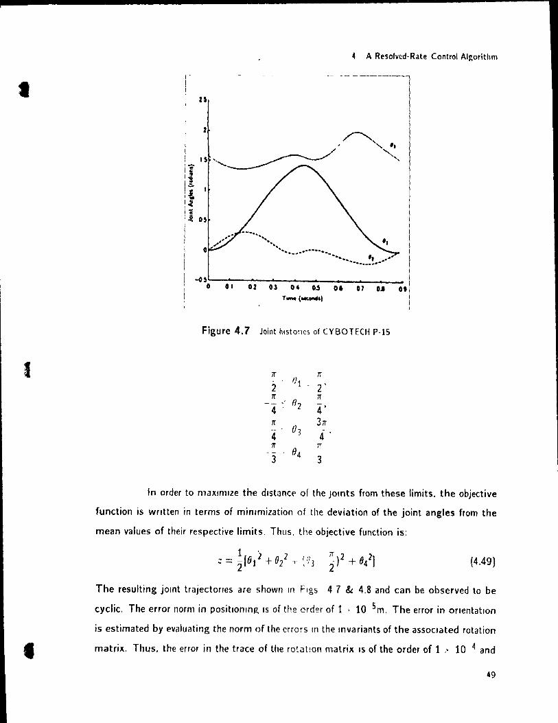
1
1
4 A Resolv~d-Rate Control Aigorithm
r -- - - --------,
n
2
1 S
! 1
!1 I~
Il 05
1 -- ....... ,
" " .. "........ . ........ .. .. _.-. -... ....... ,.... '1 .. _ ......... -05~~~~--~~ ________________ __
o 01 02 Ol 04 O~ 01 07 0.1 Of T_(--'I)
Figure 4.7 Joint histones of CYBOTECH P-15
7r 7r
2 f) 1
2 ' 7r
82 7r
4 - 4' 7r
°3 371"
-- -4 4 7r
f}4 il"
3 3
ln order to maxlmlze the d.stancE' of the JOints from these limits. the objective
function is wntten in terms of minlmization of the deviation of the joint angles from the
mean values of their respective limits. Thlls, the objective function is:
(4.49)
The resulting jOint trajectorres are shown I!l F Igs 4 7 & 4,8 and can be observed to be
cyclic, The error norm in positlOnrng IS of the crder of 1 . 10 Sm, The error in OrientatIon
is estimated by evaluating the notm of the errors III the rnvariants of the assoclated rotation
matr;x, Thus. the error in the trace of the rotatlOn matrix .5 of the arder of 1 .' 10 4 and
49
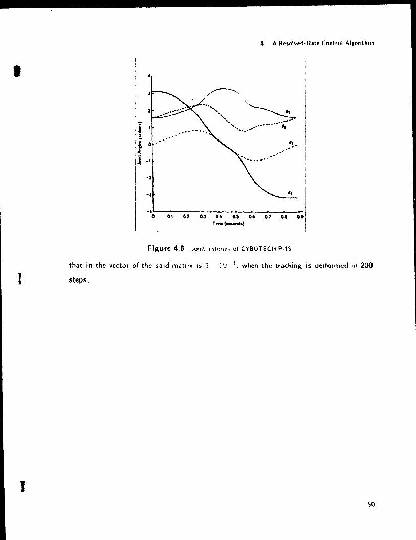
1
1
J
•
-2
-)
4 A Rt'solved·Ralt' Control Aigorlthm
'~ . . '" .' -",'
-.~--~------~------~--~--------~ o 0' Of 0.3 h U 01 07 U .. T_(..-4.)
Figure 4.8 JOint hlstOII"'> of CVBOTECH P·IS
that in the vector of the said matriT. is 1 1 a 3. when the tracking IS performed in 200
steps.
(
c
Chapter 5 Complexity Analysis
As pornted out in the last chapter. the Implementation of the resolved-rate al
gonthm using the veloclty Jacoblan 15 advantageous as compared to the scheme where
the displacement Jacobian 15 used. owmg to the fact that the former is easier to compute.
Moreover. the usage of the dlsplacement Jacoblan demands that the mdependent row vec
tors of the Jacoblan be obtamed by sorne numencal procedure. wh Ile the velocity Jacoblan
metnod facihtates the isolation of these mdependent vectors at the modellmg stage itself.
Thus. the scope of his chapter IS Itmlted to analyzmg the computatlonal cornplexity of the
resolved-rate control scheme usmg the veloclty Jacoblan.
ln what follows. multiplicatIOns. additions and square-roots are represented by
subscrrpted At :t. and S respectlvely Aiso. subtractlons and divisions are classlfied
as addition and multiplication operations. respectlvely Obviously. the flrst step ln the
computations IS the formation of the veloclty Jacoblan K T 0 that effect. It IS assumed
that ail the computations are bemg performed wlth vector components glven ln the first
coordmate frame Thus. el IS slmply glven as (ü.o.lf. the remammg el vectors bemg
slmply the thlfd column of Pli' whlch 15 defined as Q1 Q] . Q, -1. for 1 = 1.. 11 The
calculatlon of each rotation matnx QI requlres 4 multiplications and zero additions. and
hence. ail ri QI matrices are computed wlth 41/ multiplications and zero additions. ri bemg
the number of links of the redundant mantpulator Moreover. the Il P 2 matnces can be
computed recursively usrng the following scheme (Angeles 1989)'
t
'.
5 C.oOlplcxlly Allaly~ls
(5.1 )
The computational algonthm 15 then
For 1 = 2 to 1/ do (5.2)
enddo
The product PI 1 QI IS most eftlclently computed as follows
Let P/- 1 and PI be glven as.
[ "Il Pt'}
"
13
1 PI t- P21 l'n 1']3
1'31 Pll 1'33
[ pi 1 1
, 1 Pl] 1'13 P, 1
"?3 P]l /In 1 1
PH /1 rI /13 {
Then. matnx P ( IS computed ln the followlng ~equem e
li 1 =- lill Sin O{ 1'1] <'05 (J,
l', ::c 1}21 Sin o{ lin cos (JI
l1', == 1131 Sin 0, JI)] <.os (J,
and
P~l = l'Il COS 0, + 1'12 sm (J,
1 PD = u1 cos u i + 1'13 sm 0,
, 1J13 -= !JI Sin (lI + P13 cos ° 1
(5.3)
(54)
(5.5)
(5.6)
(5 7)
(5 8)
(5.9)
(5.10)
(5.11)
«
c
1 . PB = 1'1 Sin Ql + P23 COS o'{
P~t = P31 COS (J, + P32 sin (Ji
5 Complexity Analysis
(5.12)
(5.13)
(5.14 )
(5.15)
(5.16 )
Thus. the calculation of each P, reqUires only 24 multiplications and 12 additions. leading
to the conclUSion that. for 11 jOints. thls algonthm reqUires 24(n - 1) multiplications and
12(71 - 1) additions. Pl having been obtalned at no cost
The calculatlon of ail a, veftors requires only 2n multiplications, whereas. the
r" vectors can be determlOed recurslvely by a scheme similar to the one of Horner's for
polynomial evaluatlon. as proposed by Angeles (1985). I.e ..
For l = ri - 1 ta 1 do (5.17)
endda
ln the foregolOg algorlthm. each '1 vector IS computed in the Ith coordlnate
frame Ta transfer It to the flrst frame. whlch 15 assumed to be the coordinate frame flxed
to the robot base. the followmg transformation IS performed.
(5.18)
The computation of ri can be done economlcally as follows
(5.19)
where
(5.20)
53
1
and
(5.21)
Wlth thls scheme. tht' evaluation of ail (r, Il vt'ctor<, take~ a totdl of 181/ 16 rnultlpllc,ltlol1"
and 14(1/ 1) additions The cro~~ product of e, will! r, wh,dl t,lkt·<' 6(11 1) multlpll(,lllon"
and 3(11 1) additions. Will glve ail the p,Hdrneter~ reqlllred to form the Illdtm Lomponenl
B of K If ,\11. and A" denote the total nurnbN of the multiplie ,Itlon<, ,Hld clddltlonc,.
respectively, reqUired ln the formation of th!' veloclty Jo1( Obl.Hl. K. then
.\1 J.. -::: 52t/ 46 (5.22)
and
(5.23)
The next step ln the scheme I~ the computation of the modifled vettor of
Lagrange multlpllers À' introduced in eq (4 34) ThE> sa Id vedor I~ deterrnllled a~ the least
square solution to the overdetermmed system of equatlons (4 33) As rnentloned carller.
the expltclt inverSion of K K T IS aVOlded ,lI1d Hou<,rholder relle( t IOns die ue;,ed tnstE'ad, to
render the matnx K 7 upper trtangular (Golub and V,IIl Loan 1983. AnJ?;C'I('<, ,Hld M,wu 1989)
The triangulation of an 71 . 7fI matrlx hy th!" ",ud nH'thod H'qUlre" \II Illllltlplitations, .1,
additions and .'-,1 square root,> (Anderson 1987). wherr
.\f1~~11111""111(311 t 3 /II)J 3
and
A, = ml5 + m(671 --t 3 2m)) fi
(5,24 )
(5.25)
(5.26)
The application of Tf1 Householder reflectlons to the TI dimenslOnal vec tor \':~ npede;, \f,
multiplications and AI additions. where
.\1/ - 7fI(211 1fI t 3) (5.27)
and
A, - m(2n 111 +- 1) (5.28)
~4

t
5 Complexity Analysis
Then. vector A" is obtalned by back substitution. which involves M~ multiplications and
A. additions. where
.\1.~ = A.< = m(m + 1)/2 (5.29)
Hence. the total number of multiplications and additions required to solve the overdeter
mined system of equatlons is AL and A" respectively. where
(5.30)
and
(5.31 )
The total number of square roots. 80 • is equal to St given above
The evaluatlon of ". requires the formation of a third-rank tensor given ln
eq (4.39). For the evaluation of aA,' ae. cross products of three-dimensional vectors have
to be obtained. which requires 6 multiplicatIOns and 3 additions. each. Since the cross
product of any vector wlth el does not reqUire any computations. becau"~ ail the operation~
are performed ln the flrst reference frame. which IS flxed to the base of the robot. there IS
a saving ln the number of computations Thus. if AfA and .4}\ represent the total number
of multiplications and additions reqUired for the evaluatlon of aA,' df). then.
AfA = 3n(n <- 3) + 6 (5.32)
and
A}\=(n 2)(3n- 3)12 (5.33)
Moreover. the computation of each vector element of as / ail reqUlres the evalu
ation of only a single vector product since e1 ) fi for 1 = 1 to 11. have already been computed
dunng the formation of K. The computation of aB 1 ae thus reqUlres AIR products and AH
additions where
MB := 3n(n 1) (5.34)
and
AB = 3n{n -1)/2 (5.35 )
55

J
5 Complcxity Analysis
Ali that is left now in the process of the evaluatlon of A'" is the multiplication of the thlrd
rank tensor iJt< / ail with the modlfied vector of Lagrange multlpllers. T 0 that effect. It i~
convenlent to partition the said vector lOto two 3-dlmensional vectors Ai and '\2 such that·
(~~)TA' + (dB)T,\* = ,,-dO 1 cJO '
(5.36)
Then. the formation of the Tl )' TI matnx (dA ,cJO) T). i requires At t := 311 (11 1) 12 multiplica
tions and Al = n(rI--l) additions On the other hand. the computation of (iJB/aiJ)I1'Pi
needs M, = 3n(15 - 11)/2 multiplications and A2 = 11(15 1/) additions Moreover. for
the formation of A~. the two ri ' TI matrices have to be added. whlch takes an additional
ATi = 712 operations. Now. rnatrix M* IS evaluated by adding \,2 z to A * Since the entries
of the Hessian matnx \,2 z depend upon the functlOn that the user wishes to mmimlze. we
cannot predlct the exact number of addltlon~ Involved ln the formation of the matnx M'
However. if the objective function chosen is such that none of the entnes of the Hesslan
matrix are zero. then. ri' additions are reqUired to evaluate matrix M*.
The tWist vector IS computed wlth only 32 multiplications. 16 additions and 1
square root (Angeles et al 1987).
The Joint rates and the time derivatlves of the modlfJed Lagrange multipllers can
now be found by solvlng the Imear system of equations (4 36) through the application of the
LU-decomposltlon algonthm. requiring the decomposltion of the (11 + 1rI) . 1 ri + Tf1) matnx
coeffiCient lOto lower and upper trlangular factors The process of LU decomposltlon and
the subsequent back and forward substitution takes Mlu multiplicatIOns and A/u additions.
where
Mlu = (n + m)l2(n + w)2 + 9(n + TrI + 1)]/6 (5.37)
and
A/u = (n + m)l(n + m)2 + 3(11 + tri 4))/3 (5.38)
Hence. the total number of operations reqUlred for the evaluatlon of the joint
rates is'
,
t 5 Complexity Analysis
.\.-ltot =- [211 3 + (6m + 45)11 2 + (6m 2 + 30117 1'- 375)11 + 2m3 + 6m2 + 30rn + 144] /6
(5.39)
At"t = [211 3 + (6m"T 36)11 2 -+ (6m 2
ï 24m + 180)n + 2m 3 + 3m2 - 15m + 54] 16
(5.40)
ln order to have a feeling of the computatlonal complexlty Involved. the number
of computations reqUired for evaluatmg the joint rates of a seven-a,(is. spatial posltlOnmg
and onenting manipulator were determtned. Moreover. to do away with the arbltranness
assoclated wlth the number of computations required for the evaluation of matrlx Ma. we
choose to minimlze the followtng objective funetion
(5.41)
where (JI and 0; for 1 = 1, .. ,4 are nothing but the joint angles and the reference values
from whlch the deviation of these JOtnt angles is to be mtnlmlzed. respectively. These
reference values represent the mean of the JOint Itmlts of each Jomt, as rn Example 4.3 ln
this ca~e. the evaluatlon of the Jomt rates and the tlme derivatlve of modlfied Lagrange
multlphers at the starttng pornt on the trajectory reqUires 1837 multiplications and 1371
additions. For subsequent poses along the conttnuous traJectory. the number of computa
tions can be reduced to 1532 multiplications and 1094 additions If the joint rates and the
rdtes of the modlfled Lagrange multiplters are mtegrated over time
57
1
Chapter 6 Off-Line Trajectory Planning for Collision Avoidance
6.1 Introduction
ln practlcal situations. a robot may be required to work JO a spaee cluttered wlth
difTerent obJects Any robotle application ln such surroundings will demand that the task
be performed precisely. wlthout the robot coillding wlth the obJects A robotlc mampulator
possessing kmematlc redundancy paves the way for the satisfactory compllance wlth the
sa Id requirements The extra degree(s) of freedom of the redundant manlpulators can
be very effectlvely utillzed for the purpose of colliSion avoldance. as pomted out by sorne
researchers (Klein 1984. Freund 1977)
Researchers have pnmarily dealt wlth the problem of obstacle aVOIdance and
path plannmg in the two ways Iisted below
• The initiaI and the final pose of the EE are speclf,ed and a path between these
two poses. such that the mampulator does not Interfere wlth the objects in the
workspace. IS to be computed ThiS problern is baslcally of the plck-and-place
type
• The mdnipulator links, are reqUired to keep away from the obstacles whlle the
end-effector tracks a specified contmuous trajectory.
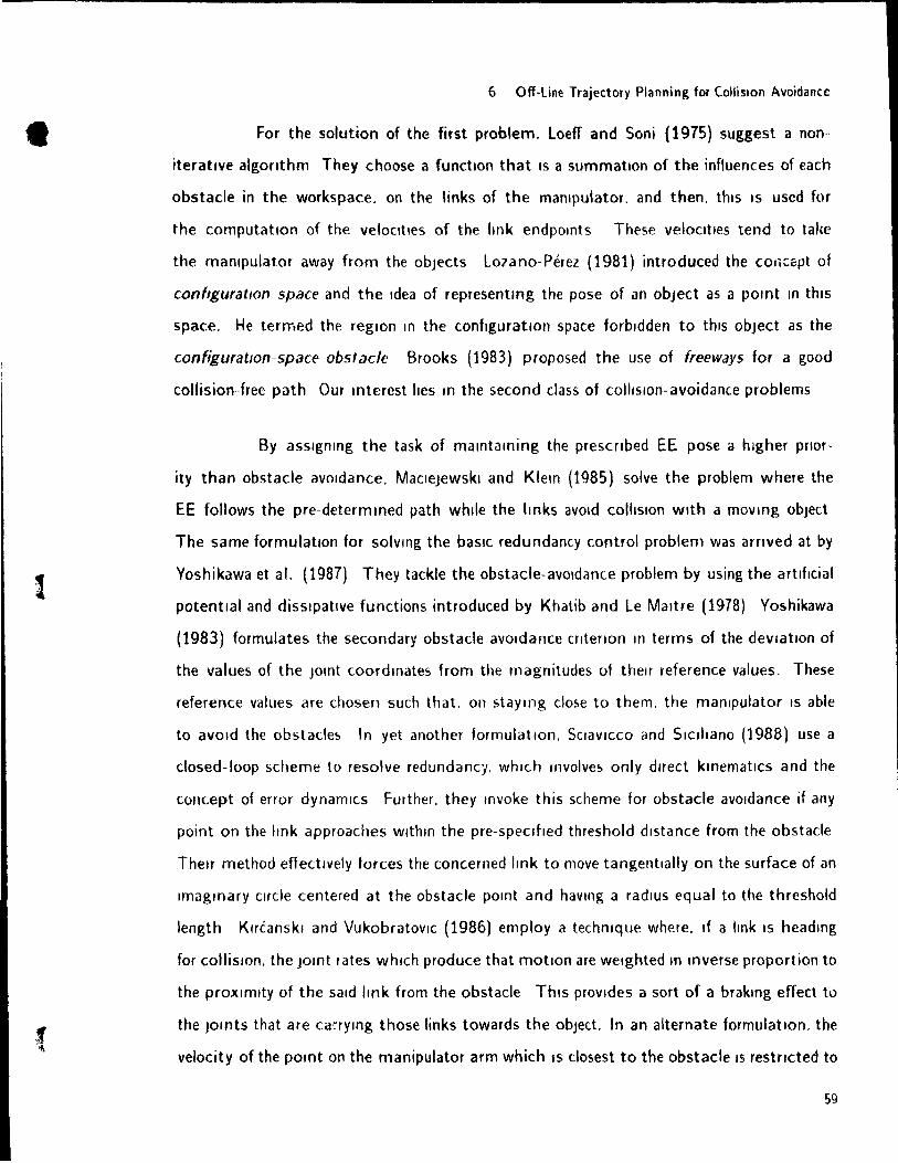
1
6 Off-Une Trajectory Planning for Collision Avoidance
For the solution of the first problem, Loeff and Soni (1975) suggest a non
iteratlve algonthm They choose a functlon that IS a summatlon of the influences of eaeh
obstacle in the workspace, on the links of the mampulator. and then, thls IS used for
the computation of the veloCltles of the hnk endpolnts These veloclt,es tend to tal,e
the mantpulator away from the obJects Lozano-Pérez (1981) introduced the COII~épt of
configuratIOn space and the Idea of representmg the pose of an obJect as a pomt ln thls
space. He termed the reglon ln the conftguratlon space forb,dden to thls obJect as the
configuratlon-space obstacle Brooks (1983) proposed the use of freeways for a good
collision··free path Our mterest Iles ln the second class of collision-avoidance problems
By asslgnmg the task of mamtaming the prescnbed EE pose a hlgher pnor
ity than obstacle avoldance. Mac,eJewskl and Klein (1985) solve the problem where the
EE follows the pre-determmed path whde the Imks aVOId collision wlth a movmg obJect
The same formulation for solvmg the basIc redundancy control problem was arnved at by
Yoshikawa et al. (1987) They tackle the obstacle-avoldance problem by using the art,flcial
potentlal and diSSipative functions introduced by Khatib and Le Maitre (1978) Yoshikawa
(1983) formulates the secondary obstacle avoldance wtenon III terms of the devratlOn of
the values of the JOint coordmates from the magnitudes of thelf reference values. These
reference values are chosen such that. on staymg close to them, the man,pulator 's able
to avold the obstacles ln yet another formulatIon. Sc,avlcco and S,cJllano (1988) use a
closed-Ioop scheme to resolve redundancy, whlch Involve~ only direct kmematlcs and the
concept of error dynallllcs Further, the y Invoke this scheme for obstacle avo,dance if any
point on the hnk approaches wlthln the pre-spE'Clfled threshold distance from the obstacle
Thelr method effect.vely forces the concerned Imk to move tangentlally on the surface of an
Imagmary Clfcle centered at the obstacle pOint and havmg a radiUS equal to the threshold
length Klréanskr and VukobratovlC (1986) employa technique where, If a "nk IS headlng
for collisIOn, the JOlOt lates whlch produce that motion are welghted ln IOverse proportion to
the prO){\mlty of the sa,d "nk trom the obstacle ThiS provldes a sort of a brakmg effect to
the JOints that are ca~rymg those links towards the obJect. In an alternate formulation, the
velocity of the palOt on the manipulator arm which 15 closest to the obstacle IS restncted to
59
1
•
6 Off-Une Trajectory Plannin!l, for Collision Avoldanc{!
a certain value speclfled by higher-Ievel controllers like sensors. whlch prevents Collisions
BailielUl (1986) demonstrates the eXistence of four basIc conditions for collisIon between
a three-jotnt. revolute-coupled. planar redundant manlpulator and a Clrcular obstacle The
scheme presented by 8adlelul relies on the IdentifICatIOn of these conditions and uses a
suitable performance Index that would carry the mampulator "nk!> away from the object
He uses the extended-Jacoblan technique to resolve the ktnematlc redundancy
ln thls chapter. a novel approach 15 adopted for solvtng the problem of trackmg
a closed C arteslan traJectory usmg a redundant manipulator ln such d way that the hnks
do not violate the area bounded by the curve that forms the tralectory Such a problem
IS commonplace ln a manufacturmg envlronment For Instance. It may be reqUired ta
weld or pamt the surface of a cyllllder and at the same tlme make sure that the Imks
of the manipulator performing the task do not colhde wlth the surface Itself One of the
most common methods employed for domg 50 I~ sWltc.hmg the robot mto teach mode and
recordtng the jomt-varlable histones whlle the mantpulator IS gUided manually through the
trajectory The very fact that there IS a human element Involved ln the tracktng results
m inaccurac.ies by the way of errors ln the pose of the end-effector. Hence. the alm IS
to tackle the problem at the software level. 50 that the errors ln the performance of the
task are mtnlmlzed ln tlll', thesis It 15 assumed that the traJectones are convex and that
the workspace of the maillpulator IS devold of any other obstacles apart from the convex
surface on wh/ch the traJectory Itself IS present Although the procedure IS applicable to any
convex contour. It IS Illustrated ln thls thesis by assummg a partlcu!ar elltptlcal shape. for
an ellipse IS a paradlgm of convex contours Flrst. an algebralC formulation IS proposed for
the planar trajectory tracktng wlth a three-Itnk. revolute-coupled. redundant manlpulator
The mathematlcal treatment of the problem 15 based on (ertaln assumptions and cnterla
which help define 'collision aVOIdance'
The problem IS made computatlonally effiCient by uSlng a Judlcious comblnatlon
of a nonlmear iteratlve procedure for constramed optlmlzatlon and a resolved-rate control
algorrthm As pointed out ln the tntroductory chapter of this thesis. any optlmlzatlOn
60
(
f
6 Off-Une Trajectory Planning for Collision Avoidance
method that deals with the problem at the joint-coordinate level has the inherent drawback
of bemg computatlonally expenslve as compared to an algorithm that deals with the same
problem at the Jomt-rate level For the problem at hand. the proposed scheme demands
that exact solutions at some sample pOints around the traJectory be obtamed at the Joint
coordlnate level However. a compromise IS attempted between the extent of usage of
the iteratlve process and the resolved-rate control algorlthm to make the complete off-Ime
procedure less tedlous and computatlonally economlcal
The manlpulator configurations at a few sample points around the Cartesian
path of the EE are computed usmg the orthogonal-decomposition algorlthm (Angeles. An
derson and Gasselin 1987) Estlmates of the JOint angles at the other (arteslan pOints
on the traJectory are then evaluated usmg cublc-splme interpolation These estlmates are
subsequently used to search for the accurate configuration ln the nelghborhood. using the
resolved-rate control algorlthm proposed in Chapter 4. modifled to accommodate time
vary Ing performance mdlces
ln the later part of the chapter. Ideas used earller for the kinematic inverSion
for the planar manlpulator have been extended. under certain conditions. to tnc\ude a wider
range of general orthogonal manlpulators capable of posrng the end-effector m the three
dlmenslonal Carteslan space ThiS extension IS /llustrated by an example where a mampu
lator wlth the CYBOTECH P-15 architecture Îs employed for the requued task
6.2 Collision Avoidance with a Planar Manipulator
6.2.1 Collision-Avoidance Policy
It IS ev/dent that. as long as the manapulator configuration is such that none
of the Itnks touches the surface of the obstacle. the condItIOn of obstacle avo/dance IS
actually met Thus. the feaslble solutions to the obstacle-avoidance problem constitute
the complement to the set of configurations that lead to collision. in the universal set that
61
,
1
1
6 Off·line Trajettory Planning for Collision Avoidance
- ~ -~--~-- - - - ------y
Figure 6.1 Third Iink farthc~t (rom ob<;tacle Obstacle shown as the shadcd rcgion
comprises ail the homogeneous sollJtions of the manipulator in the configuration space.
Since there may be an infinite numher of such acceptable solutions possible. the problem
now is one of chooslng a partlcular ronflgur<1tlon out of the infinite feasible ones For that
purpose. certain conditions have ta be deflned whlch will act as gUldelines ln the process
of selection of the optimum configui citIon Thereafter. these conditions will be formulated
algebraically and implemented in tht collision-avoidance scheme.
Since the scheme relies cn prior kllowledge of the environment. it is imperative
that an acceptable model of the obstacle be ndopted at the outset. To that effeet. the
obstacle is defined as the area envelopcd by the closed. convex Cartesian trajectory to
be tracked by the manipulator For the purpose of illustrating the procedure. the planar
obstacle is assumed to have an elllp~ltal sh,lpe However. It will immediately be realized
that the Jast link of the manipulator may 'lIolJte the boundary of the ellipse. wh/ch brings
about the need ta establtsh the rule:.. of cQIl'slon-avoidance as follows'
• The Ja!>t link of the arm l1li111 be f'.lr~hest from collision when the axis of the said
link is collinear with the pannai v"ctor of the traJectory at the point where the
62
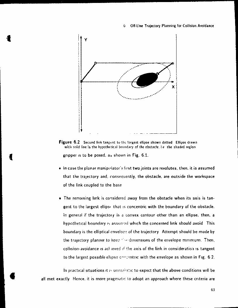
t
t
6 Off-Une Trajectory Planning for Collision Avoidance
y
Figure 6.2 Second link tang.:nt to tht: I,ugest ellipse shown dotted Ellipse drawn with solid line is the hypothnical bOllllditry of the obstacle. je the shaded region
gripper IS to be posed. a~ shown in Fig. 6.1.
• In case the planar manipldator's flrst two joints are revolutes. then. it is assumed
that the traJectory and. consequently. the obstacle. are outside the workspace
of the link cou pied to the base
• The remaming "nk is cO'1sidercd away tram the obstacle when its axis is tan
gent to the largest ellips' that IS concentric with the boundary of the obstacle.
ln general if the trajector'l is é) tonvex contour other than an ellipse. then, a
hypothetlcal boundary l', aSSllll''èd whlch the concerned Imk should avoid This
boundary is the elliptical ('nvelop,: of the trajectory Attempt should be made by
the traJectory planner to keei~ 1 :'"> dimenSions of the envelope minimum. Then,
coilision-avoidance IS aclleved If the axis of the link in consideration IS tangent
ta the largest pOSSible ellipse cr'''::~ntrlc with the envelope as shown in Fig. 62.
ln practlcal situations It l'· unre(11Is~IC to expect that the above conditions will be
ail met exactly Hence. it is more pragmatlc to adopt an approach where these Criteria are
63
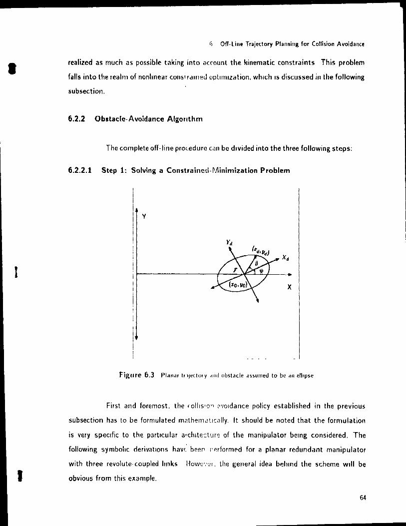
1
1
1
li OfT-Line Trajectory Planning for Collision Avoidance
realized as much as possible taking into i1crount the kinematic constraints This problem
falls into the realm of nonlmear con~'rdllled optllllization. whlch 15 discussed in the following
subsection.
6.2.2 Obstacle-Avoidance Aigoflthm
The complete off-line procedure CilO be dlvided into the three following steps:
6.2.2.1 Step 1: Solving a Constraincd-Minimization Problem
y
Figure 6.3 Planilr tflJectol y rllld obstacle assumed to be an ellIpse
First and foremost. the (01115'0" "'/oldance policy established in the previous
subsection has to be formulated m<lthematlçally. It should be noted tl1at the formulation
is very speCifie ta the partlcular a'chlte-:ture of the manipulator belng considered. The
following symbollc derivatlons hav'_ beef'1 1'~rformE'd for a planar redundant manipulator
with three revolute· coupled lillks Howe"".!I. the general idea behmd the scheme will be
obvious trom this e}(ample.
64
1
t
6 Off·Une Trajectory Planning for (vllision Avoidance
ln accordance with the collislon-avoidance poltcy established earlter. it ;s as
sumed that the trajectory IS posltioned such that It is outside the range of the tirst IInk
We start with the mathematlcal modelltng of the condition which will result ln the second
link bemg conftgured away trom the ellipse. accordtng to the proposed policy. The traJec
tory to be traced. and hence. the obstacle to be avaided. IS an ellipse and is assumed to be
centered at the coardinates (.rc.ya) mea'iured ln the robot base frame (X - r). Its major
aXIs rotated at an angle t· wlth respect to the X -axIs of the robot base. Fig 6 3. Then.
the equatlon of the Ime representlng the aXIs of the second Imk can be written ln terms of
the jOint angles 01 and 02 ln the followmg way
(6.1 )
From eq (6.1) the expression for y can be derived as
.r sin (01 + 02) - al sin ()2 y = - -~- - -- ----------
cos (01 + 02) (6.2)
provlded cos(Ol + 02) ::t:. 0 If COS(()l + 02} = O. then. rather than solvtng for y. eq.(61) is
solved for l
The equatlon of an ellipse expressed ln a coordmate frame 1 wlth origin at the
ellipse' s center. and axes parallel ta the pnnclpal axes of the elhpse. is evidently
2 2 .r,,- + YI=. 1 0 2 h2
(6.3)
where. (.rd .y,j) are the C.Hteslan coordtnatf;s of a pomt of the ellIpse ln the coardtnate frame
! Moreover, {l and " are the major and the mlllor semiaxes of the ellipse. respectively
Furthermore. the .r,j and Y,I coordinates can be evaluated ln the robot base frame as follows
I,i = (.1' - IO) cos 1.' + (y - YO) sin 1.' (6.4)
and
Yd =- (.1' .To) sin '/;' + (y - YO) cos 'I/J (6.5)
The points of mtersectlon of the second Imk and an ellipse concentric wlth the traJectory
are then given by substltutlllg the values of y . .Td and Yd from eqs.(6.2.6 4. & 6.5) lOto
65

1
,
6 Off-llne Trajectory Planning for Collision Avoldance
eq.(6.3) Aiso. since our intention is to determine the largest possible ellipse concentflc
wlth the trajectory. we express a in terms of b and the ratio r. defined as'
a r=
li (6.6)
Henceforth. it will be convenient to denote sm 1.'. cos '/J'. Sin (J2' Sin ((Jt + (2) and cos (Ot + (2)
by '\ . c 1," • ... 2. "'12 and ft2. respectively. Thus. the followmg equation quadratlc ln T glves
the .r-coordinate of the Intersection of the ellipse concentnc with the trajectory. and the aXIs
of the second hnk. The following symbolic derivatlons were performed usmg MACSYMA
software for algebralc manipulations
AI2 + HI + C = 0
where
_ ( 2 2 2) 2 2 (1 ",2) ( 2 2 2) 2 .4 - r cf/; + $ti 812 + - 1 c1/J s-rt c12'<'12 + 8 11 r + CV' C12
B = .. \'/ D
C =f,,'d2 -+ F 2
E =(c~ Y~ - 2c,..'>1, royo + r6'~~
1
(6.7)
(6.8)
(6.9)
(6.10)
(6.11 )
(6.12)
(6.13)
The axis of the second link is tangent to the ellipse concentric wlth the traJectory If. and
only if. the discrimmant of the above mentloned quadratlc equation is equal to zero. 1 e .
H2 -- 4AC = 0 (6.15)
66
1
1
1
6 Off·Une Trajectory Planning for Collision Avoidance
It can be noticed that eq. (6 15) 15 dependent on 81, (}2 and b Thu5. b can now be determÎned
from eq. (6 15) in terms of the tirst two joint angles. and IS given as
(6.16)
where.
(6.17)
and
(6.18)
On maxlmlzing b subject to kinematic constraints. a configuration can be obtained where
the second Itnk will be farthest from the traJectory.
The performance index that will keep the third link from colliding with the
trajectory is simpler to obtain. To that effect the eccentric angle of the ellipse is defined
as the angle between the radius vector from the Of/gin of the 1 frame to a pOint on the
ellipse. and the Xd axis ThiS angle Î::;, denoted by i'J The equation of the normal at any
pOint on the ellipse whose eccentnc angle IS 3. In the J frame. can be glVen as
(6.19)
Then. the si ope of the normal ln the base frame is evaluated c3S
Q m = tan larctan ( b tan 3) + 'II'l (6.20)
Thus. if the slope of the axis of the thlrd Ilnk. from here on referred to as ml. 15 equal to
m. then it Will be farthest from the trajectory accordtng to the collision-avoidance policy
estabhshed earlter ln thl5 sectIon.
Therefore. on tncorporattng the performance indices derived above lOto an ob
jectIve function z and then minimizing It subject to the klOematic constraints. the followmg
problem IS formulated
mm l' tJ
(6.21 )
67
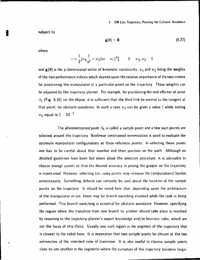
1
6 Off-Une Trajectory Planning for Collision Avoldaru:e
subJect to
g(O) = 0 (6.22)
where
1 1 2 l' = [1l't'2 + 1l'2(m IIld].
2 b o 11'1,11'2' 1
and g(O} is the p-dlmenslOnal vector of klnematlC constramts. wl and w2 being the welghts
of the two performance indices whlch depend upon the relative Importance of the two crltena
for posltlonmg the manipulator at a partic.ular pOint on the traJectory These weights can
be adJusted by the traJectory planner For example. for positionlng the end-efTector at pOint
85 (Fig 6.16) on the ellipse. It is sufflclent that the thlrd IInk be normal to the tangent at
that pOint. for obstac\e-avOidance ln such a case U'] can be glven a value 1 while settlng
11'1 equal ta 1 . 10 3
The aforementloned pOint 85 IS ca lied a sample pOint and a few such pOints are
selected around the trajectory Nonlinear constralned mmlmization IS used to evaluate the
optimum mampulator configurations at these reference pOints. In ~electll1g these pOints
one héts ta be careful about their number and thelr position on the path Although no
detailed guideltnes have been laid down about the selection procedure. It IS advisable ta
choose enough pOints 50 that the deslred accuracy ln posing the gnpper on the traJectory
IS malntamed However. ~electll1g tao, nany pOints may II1crease the computatlOnal burden
unnecessarlly Somethmg deftnlte can certamly be sald about the location of the sample
pOints on the traJectory It should be noteu here that, dependlng upon the architecture
of the manlpulator ln use, there rnay be branch sWltchmg Involved whlle the ta5k IS bemg
performed. ThiS branch sWltchlng 15 essentlal for obstacle aVOIdance However. specifymg
the region where the transition from one branch to anotner should take place IS resolved
by resortmg ta the trajectory-planner' 5 expert kn0wledge and / or heunstlC rules. whlch are
not the focus of this thesis Usually one such reglon I~I the segment of the traJectory that
is close st to the robot base It IS imperatlve that two sample pOints be chosen at the two
extremltles of the mtended zone of transitIOn It is also useful to choose sample points
close to one another ln the segments where the curvature of the traJec.tory becomes larger.
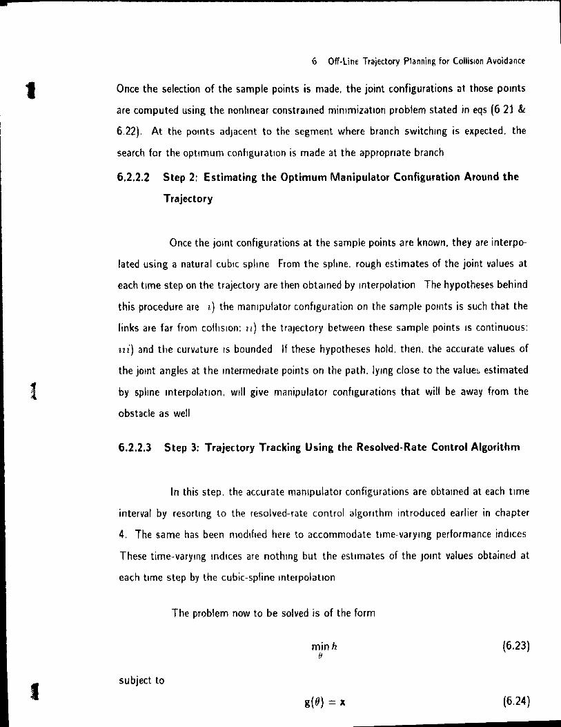
1
1
6 Off-Une Trajectory Planning for Collision Avoidance
Once the selection of the sample points is made. the joint configurations at those pOints
are computed using the nonlmear eonstralned minlmizatlon problem stated in eqs (6 21 &
6.22). At the pomts adjacent to the segment where branch switchmg is expected. the
search for the optimum configuration is made at the appropnate branch
6.2.2.2 Step 2: Estimating the Optimum Manipulator Configuration Around the
Trajectory
Once the jomt configurations at the sam pie points are known. they are interpo
lated using a natural eu bic spline From the spline. rough estimates of the joint values at
each tlme step on the trajectory are then obtamed by mterpolation The hypotheses behind
this procedure are 1,) the manlpulator configuration on the sam pie pOlllts is such that the
links are far from colliSion: n) the traJectory between these sample points 15 continuous:
ui) and the curvdture 15 bounded If these hypotheses hold. then. the accurate values of
the jomt angles at the mtermedlate points on the path. Iymg close to the value~ estimated
by spline mterpolatlon. will give manipulator configurations that will be away from the
obstacle as weil
6.2.2.3 Step 3: Trajeetory Tracking Using the Resolved-Rate Control Algorithm
ln this step. the accurate manlpulator configurations are obtamed at each tlme
interval by resortmg to the resolved-rate control algonthm introduced earlier in chapter
4. The same has been modlfled here to accommodate tlme-varymg performance indices
These time-varymg indices are nothlng but the estlmates of the JOint values obtained at
eaeh tlme step by the cubic-spline interpolation
subject to
The problem now to be solved is of the form
minh (j
g(O) = x
(6.23)
(6.24)

1
6 Off-Line Trajectory Planning for ColliSion Avoidancc
where.
and
f = 0(/) (}"(t) (6.25)
(}* (t) bemg the n -dimenslonal vector of the estimates of the joint variables at eath time
interval. T 0 obtain the assoCiated resolved-rate control algorithm. an augmented function
(' IS formed as shown below'
(' = h + À T (g - x) (6.26)
Now. the fHst-order normaltty conditions are obtatned by taking the partial derivatives of ~
with respect to (J as in eq (4.5). On difTerentlatmg the flrst-order normahty conditions along
with the klllematic constratnts wlth respect to time and forming a linear set of equations
analogous to eq. (4.24). the following algorithm IS obtained
(6.27)
where J is the p x n mampulator Jacobian. whereas À represents the p-dimensional vector
of Lagrange multiphers. (J* obviously l>emg the rate of the joint estlmates which can be
dJrectly evaluated wlth a first-order accuracy from the spline-interpolated values of the joint
angles Moreover. matllx M 15 defmed as follows.
(6.28)
The joint configurations at the next time step can thus be computed by mtegrating the
joint rates over the time mterval.
As mentioned earlier. for this problem of obstacle avoidance. It is Imperative that
the manipulator change branches at least once during the course of trackmg the trajectory.
At such an occurrence the manipulator loses a redundant degree of freedom. Depending on
the nature of the trajectory. a reglon can be estimated heuristically where such a transition
should take place. but it 15 not an easy task to determllle exactly the pOint where it should
occur This problem IS slmplifled by the procedure adopted ln thls chapter ln the example
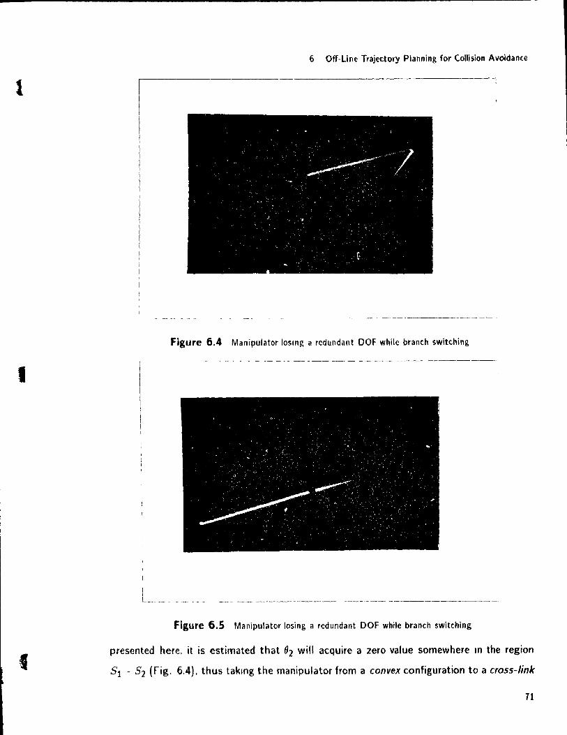
t
1
6 Off-Une Trajectory Planning for Collision Avoidance
- - ---------------
Figure 6.4 Manipulator losing a redundant DOF while branch switching
1 L _________ _
Figure 6.5 Manipulator losing a redundant DOF while branch switching
presented here. it is estimated that (J2 will acquire a zero value somewhere ln the reglon
S1 -- 52 (rig. 6.4). th us taklng the manipulator from a convex configuration to a cross-link
71
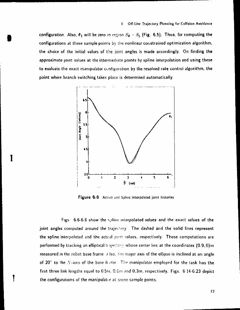
1
1
T
6 Off· Une Traje<.tory Planning for Collision Avoidance
configuration. Also. 93 will be zero ln reg,ton 8, _. 55 (Fig. 6.5). Thus. for computing the
configurations at these sample points by the nonlinear cOlistrained optimization algorithm,
the choice of the initial values of t!~e joint angles is made accordingly. On finding the
approximate JOint values at the intermedlê\te pOints by spline interpolation and using these
to evaluate the exact mampulator c(,nflguratlon by the resolved-rate control algorithm, the
point where branch switching takes place is determined automatically.
l.5'---......... --~_ ....... _--'----'---_""O'-
o 2 3 ~ 6
~ (roc!)
Figure 6.6 Act'f;)1 and Spline interpolated joint histories
Figs 6.6-6.8 show the ,.~)Iille IIlterpolated values and the exact values of the
joint angles computed iHound the trajec' ory The dashed an-:f the sol id lines represent
the spline interpolated and the actl!t11 J0"1~ values. respectively. These computations are
performed by tracktng an elliptlcal tl 1J"~'::c'~' whose center Iles at the coordinates (0.9,O)m
measured in the robot base frame J. 150. 1 il~ major axis of the ellipse is inclined at an angle
of 20" to the .Y -axIs of the base fr .me Th!' nlanipulator employed for the task has the
first three link lengths equal to D.Sm. a.cm (lnd O.3m. respectively. Figs. 6 14-6.23 depict
the configurations of the manipulatlJr at some sample points.
72
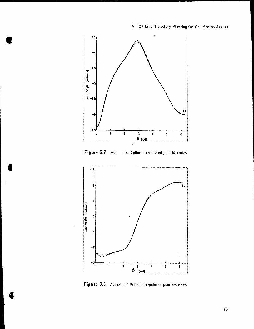
6 Off-Une Trajectory Planning for Collision Avoidance
l 1
-.15
-4
-45
-5
2 3 4 6 ~ (rad)
--~- - - ------- - -
Figure 6.1 Ac!t l,JiJel Spline interpolated joint histories
. l
-;;-r: .. 1
1"::' 0
I~ c: cl:
ë a -1 ....,
-JL---~----~ ____ ~ ____ ~ ____ ~ __ ~ ___ o 2 J 4 6
~ (rCld)
Figtlr~ 6,8 ACLI,ll ~,,(I SJ)linc intcrpolatcd JOlllt histories
73
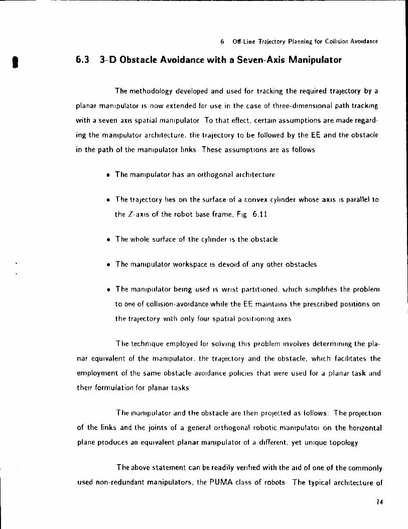
1
6 Off-Line Trajectory Planning for Collision AVOIdance
6.3 3-D Obstacle Avoidance with a Seven-Axis Manipulator
The methodology developed and used for tracking the required trajectory by a
planar manlpulator IS now extended for use in the case of three-dlmenslonal path trackrng
with a sevenaxls spatial mampulator To that ~ffect. certain assumptions are made regard
ing the manrpulator architecture. the trajectory to be followed by the EE and the obstacle
in the path of the manlpulator Imks These assumptlons are as follows
• The manrpulator has an orthogonal architecture
• The traJectory Iles on the surface of a convex cyhnder whose aXIs IS parallel to
the Z- aXIs of the robot base frame. Fig 6.11
• The whole surface of the cylrnder IS the obstacle
• The manrpulator workspace IS devold of any other obstacles
• The manlpulator berng used IS wnst partltloned .... "hlch simplifies the problem
to one of collislon-avoldance whlle the EE marntarns the prescribed positions on
the traJectory wlth only four spatial posltlonlng axe~
The technique employed for solvlI1g thls problem Involves determrnmg the pla
nar equlvalent of the mampulator. the trajectory and the obstacle. whlch facllltates the
employment of the sa me obstade-avoldance poltcies that were used for a planar task and
thelr formulation for planar tasks
The manrpulator and the obstacle are then proJected as tollows: The projection
of the links and the joints of a general orthogonal robotic manrpulatOi on the hOrizontal
plane produces an equrvalent planar mantpulator of a dlfferent. yet unique topology
The above statement can be readily venfled with the ald of one of the commonly
used non-redundant manipulators. the PUMA class of robots The typical architecture of
74
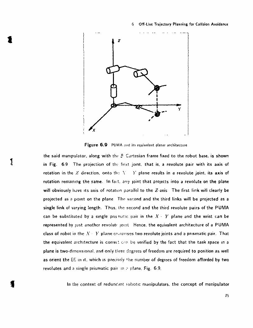
1
l
1
6 Off-Une Trajectory Planning for Collision Avoida/lce
z
y
Figure 6.9 PUMA .100 its equivalcnt planar architecture
the said maOlpulator. along with th(· E Cartesian frame fixed to the robot base. is shown
in Fig. 6.9 The projection of th~· flrst jomt. that is. a revolute pair with its axis of
rotation in the X dIrection. onto th: \' r plane results in a revolute joint. its axis of
rotation remalntng the same. In fal t. (lny Joint that proJects into a revolute on the plane
will obviously hJve Its axis of rotatIon parallel to the Z-axis The first link will clearly be
projected as il pOint on the plane The ser:ond and the third links will be projected as a
single link of varying length. Thus. the second and the third revolute pairs of the PUMA
can be substituted by a single prIS 1l.1ttc pair in the X - Y plane and the wrist can be
represented by Just another revolutt Jotnl Hence. the equivalent architecture of a PUMA
class of robot in the X - }' plane CC'IIHnlSeS two revolute joints and a pnsmatic pair. That
the equivalent archItecture is corree t ç.'11 be verified by the fact that the task space ln a
plane is two-dirnenslonal. and only three degrees of freedom are required to position as weil
as orient the EE 111 It. which IS prec.j"nly the number of degrees of freedom afforded by two
revoll.ltes and <t single prismatic pair ln .' plane, Fig. 6.9.
ln the context of redum~.lnt /Obotlc manipulators. the concept of manipulator
75
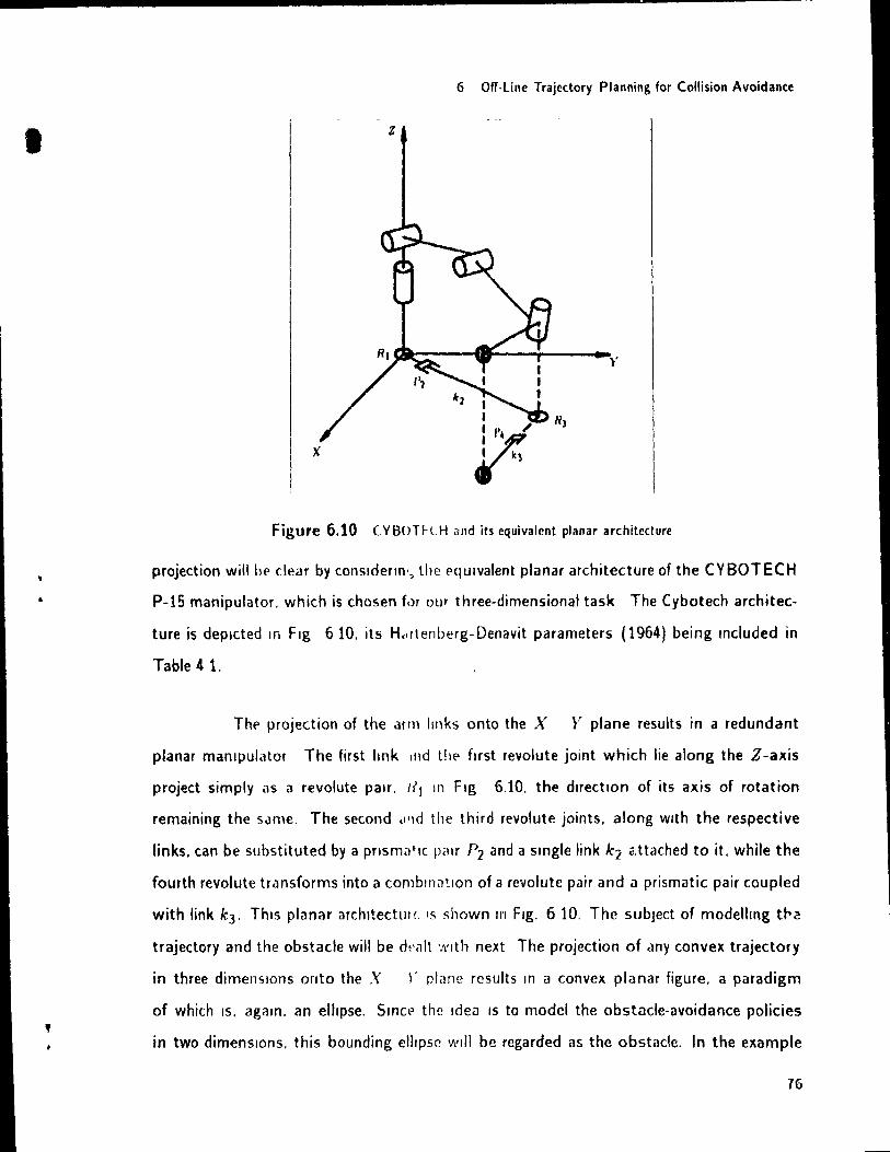
1
•
,
6 Off·line Trajectory Planning for Collision Avoidance
z
1 1 1 l'l / v:
)'
Figure 6.10 CYBOTtlH and its equivalcnt planar architecture
projection willlH' clear by conslderlO" the PClulvalent planar architecture of the CYBOTECH
P-15 manipulator, which is ch os en for our three-dimensional task The Cybotech architec
ture is deplcted ln Fig 610, its H.,rtenberg-Denavit parameters (1964) being mcluded in
Table 4 l,
Thf' projection of the arm links onto the X Y plane reslJlts in a redundant
planar manlpulator The first "nk Illd thE' fJrst revolute joint which lie along the Z -axis
project simply as a revolute pair, Itj 1f1 Fig 6.10, the directIOn of its axis of rotation
remaining the SJme. The second <l'Id the third revolute joints, along wlth the respective
links, can be substituted by a pnsmtltlc pair P2 and a smgle link kt a.ttached to it. while the
fourth revolute transforms into a comblntl~lon of a revolute pair and a prismatic pair coupled
with link k3' ThIS planar archltectulL IS shown /1'1 Fig. 610. The subJect of modellmg tr2
trajectory and the obstacle will be d!'illt 'Nlth next The projection of ,lnY convex trajectory
in three dimensIOns onto the X r plilne results ln a convex planar figure, a paradigm
of which IS, agéltn, an ellipse. Slnet> the Idea IS ta model the obstacle-avoidance policies
in two dimensions, this bounding ellipse will be regarded as the obstacle. In the example
16
1
f
6 Off Une TraJectory Planning for Collision Avoidance
considered here. the trajectory is an ellipse on the surface of an elhptlcal cyllnder. Hence.
the projection of this elhptical traJectory onto the X - Y plane is nothmg but the elliptlcal
dlrectrix of the cyhnder and the representatlon of the obstacle 10 the plane will obviously
be the same
Smce redundancy 15 only ln the links constltuting the arm-tlrst four axis-of
the Cybotech mantpulator. It IS only the hrst four JOints that can be used for the task of
colllslon-avOidance Hence. the objective reduces to obtammg the deslred position of the
WrJst ln such a manner that the links are as far away as possihle from collision
Now. the formulation of the colliston-avoidance pohcies for the f,rst three IlOks
can be accomplished ln two dimensions. 1 e . the planar eqUivalent of the manipulator ln
consideratIon can be mad~ to avold the planar equlvalent of the obstacle. whlle the klne
matlc constraints are still formulated ln three-dlmensional task space Thus. the collision
avoldallce polleles established for the planar redundant manipulator will still be applicable
Consldermg the planar representation, It is obvlous that the second and thlrd
Imks of the Cybotech Will be away from the obstacle If the aXIs of the Imk "2 IS tangent
to the b'ggest possible ellipse concentric with the projection of the trajectory ln the same
vem. the fourth Imk remalns away from the cylmder surface as long as Its aXIs IS colhnear
wlth the unit normal vector of the trajectory. at the pOint where the end-effector IS to be
posltloned
If the Imks replesent stralght-Ime segments, then. the aXIs of k 2 IS colhnear
wlth the followmg Ime
y l tan 01 = 0 (6.29)
The projection of the traJectory IS nothmg but the well-known equation of the
ellipse given ln eq (63) l'J and Yd are the points on the projection of the traJectory.
correspondmg to the points T r and Yr on the actual traJectory. Fig 6.11 Also. the
expression relating the coordinate frame of the ellipse and the robot base Cartesian frame
IS as given in eqs.(6 4 & 6.5)
77
1
l 1
6 Off-Ulle Trajcctory Planning for Collision Avoidante
v
Figure 6.11 Tt dl dOl V IfI 3-dirnensional Cartcslall space
On ~ubstltuting the valu of,l/ from eq (629) into eqs.(6_4 & 6_5). the repre
sentation of r,/ and Yd in terms of .1 IS cbtalned If 81 is 'Tf /2. then. eq.(6 29) can be solved
for x and substltuted ln eqs (6 4 & l, ::!
TI1<' relation in terms of '0' '" -.ubstltuted lOto the equatlon of the ellipse. which
glves a quadratlc equatlon ln r dehlll16 the r-coordlOate of Intersection between the Ime
representing the Imk 1-:2 and the elltp..,p, l ':' .
,1 J; + n'r+ c' =- 0
The coefflcwnb 1'. IJ' and C' of tl t'î Cil t.1CJratlc equatlol1 MC glvell bclow
1 __ (.2 2 2) 2 2(1 A - (Ii, r + ,"!/.' f 1 +
B' == S",' f)"
N if __ ( 2 .TO X081
2 2 .2 ~ Il /, +... r + ( 1
'1' 'l'
(6.30)
(6.31)
(6_32)
(6.33)
78

(
c
(./ = (c2 y 2 1; 0
6 Off·llne Trajectory Planning for Collision Avoidante
(6.34)
(6.35)
Ali the symbols ln the foregomg equatlons have the same connotation as earlier. tan 81
bemg denoted by t 1 For the Ime representlng the aXIs of the Ilnk k2 to be tangent to the
ellipse m the X } C plane. the dlscrimmant of the quadratlc equation (6 30) must vanish
Hence.
Hf2 - 4..1'(," = 0 (6.36)
It should be noted that the dlscrtmlnant is a funetlon of the length of the semi-axes of the -
ellIpse Smce our alm Îs to find the largest possible ellipse to which the axis of the link k}
CJn be tangent. It seems natural ta solve eq (6 36) for the variable band then maXlmlze
the latter Thus. b assumes the followmg form wh/ch IS dependent upon the joint variable
°t (6 37)
where
(6.38)
and
(6.39)
Now. the colhslon-,woldanee condition for the fourth "nk IS denved ln the three-dlmenslonal
Carteslan space by equattng Its direction cosmes v!ith those of the unit normal vector. at
the pOint of the deslred position of the wnst on the traJectory. The dIrection cosines L;r.
Lli and Lz. of the last link. in three-dimensional workspace. are given as follows'
Lx = sgn(bs)(('''2 s 3 - c2C3)Q'''4 - $lC41
LJl = sgn(bs}(qq - (c2 C3 - 82 8 3)81 8 4]
Lz = sgn(bsH - (C2 S 3 + S2CJ)S4]
(6.40)
(6.41)
(6.42)
79
J 6 OfT-lme Trajcctory Planning for Collision AVOIdance
It should be noted that the derivations of the direction cosines are very speclfic to the
Hartenberg-Denavlt parameters glven ln Table 4.1
If the direction cosmes of the normal vector of the traJectory. at the pomt where
the end-effector IS to bf posltloned. are 1". lu and L:::. then. the nonlmear constramed
mmimlzatlon problem for obstacle-avoldance m the glven envlronment can be formulated
as
mmu
subJect to
g(O)=x (6.43)
where U IS deflned as.
(6.44 )
and g(O) x represents the kmematlC constramts ln the three-dlmenslonal Carteslan space
The JOint coordmates at the !:>ample pomts are then evaluated usmg thls nonhn
ear scheme The orthogonal-decomposltlon algonthm devised by Angeles. Anderson. and
Gasselin (1987) 15 used to Implement the optlnllzatlon problem The estlfllates for the
di'ta pomts ail around the traJectory are then obtamed by cublC- spline mterpolatlon The
estlmates and thetr rates are subsequently used m the resolved-rdte control algonthm of
eq (627) to glve the exact jOint coordmates at each tlme step on the trajectory.
ln this example. the longitudinal aXIs of the cyltnder IS parallel to the Z-axis and
mtersects the X-axIs of the robot base frame at the coordmates (1.9,O,O)m Moreover.
the trajectory is the curve formed by the mtersectlon of a plane and the cylmder The
equation of the IOtersecting plane. glven ln the robot base frame. Îs as follows
T - 5.67 z + 5.4 = 0 (6.45)
Hence. the coordinates of any pOint on the trajectory can be calculated as follows:
80
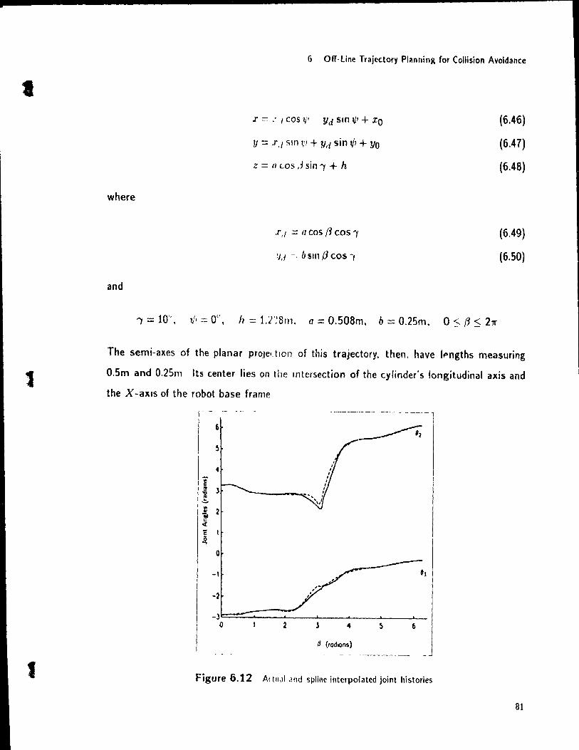
1
1
1
where
and
6 Off· Une Trajectory Planning for Collision Avoidance
r = .r 1 cos '1/' Yd sm ~, + Xo
y = r,1 sin 1/' + Y,f sin VJ + Yo
z = a LOS 11 sin..., + h
.r,1 = fi cos /1 cos...,
!J,/ =- b SlIl {J cos 1
Î = 10", V' = 0", Il = 1.2':8m. a = O.508m, b = O.25m, O:s f3:S 211'
(6.46)
(6.47)
(6.48)
(6.49)
(6.50)
The semi-axes of the planar proJe'. tlOn of this trajectory. then. have Ipngths measuring
O.Sm and O.25m Its center lies on the rntersection of the cylinder's longitudinal axis and
the X -axIs of the robot base frame
6
4
Il 2 .. c:
oc(
~ 1 ë5 ..,
o
--------1
n (rOdIOns)
Figure 6. t 2 Attll.ll .111d spline interpolated joint histories
81

1
1
6. Off-Line Trajectory Planning for Collision Avoidance
l .. c '" 2~ 1 ..
2 ..!!
1 i ....
-os~--~----~--~----~----~--~--o 2 l 4 6
t {J (IodIOns) l_~ ___ _ ________ ~ ___ ~ _________ ____l
Figure 6.13 Actual and spline interpolated joint histories
Figs. 6.12-6.13 compare the joint-variable histories obtained by the resolved
rate control algorithm and the estimated values at each time step using a natural cubic
spline. The da shed and the solid lines represent the spline interpolated estimates and the
actual values. respectively.
__________________________ ---..l
Figure 6.14 Manlpulator configuration at sample point Si
82

6 OtT-Une Trajec.tory Planning for Collision Avoidance
Figure 6.15 Manlpulator configuratIOn ilt silillple point 52
Figure 6.16 Manlpulator configuration at sample point 53
f 83
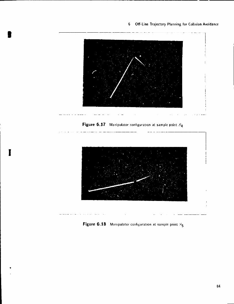
1
1
6 Off-Une Trajectory Planning for Collision Avoidance
1
1 --------- -~-,
Figure 6.17 Manipulator configuration at sam pIe point S4
l 1
Figure 6.18 Manlpulator configuratIOn at sam pie point "'5
84
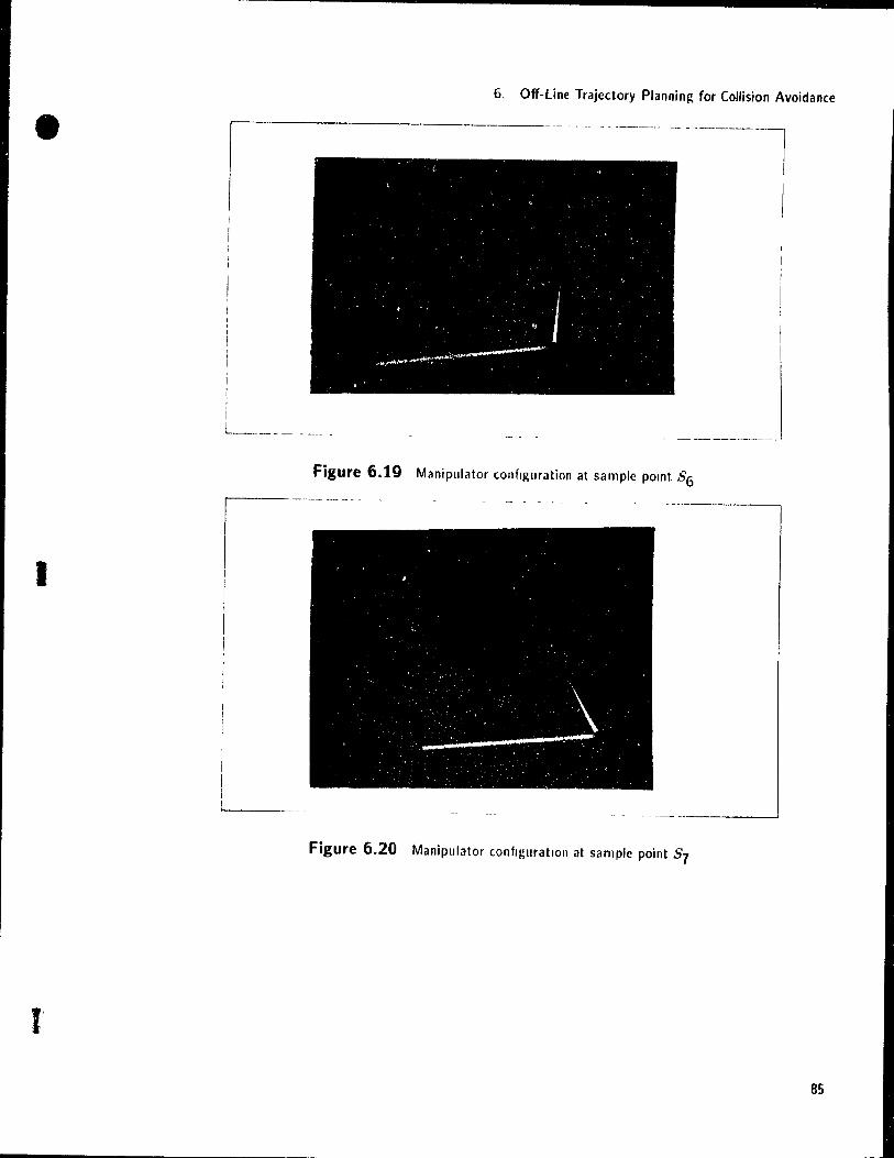
6. Off-line Trajectory Planning for Collision Avoidance
-- - --------)
1
1
i L ____________ _
Figure 6.1 9 Manipulator configuration at samplc pOint 86 r----- --- --- - __ - -- --- ._-------,
1
Figure 6.20 Manipulator configuratIOn at samplc point 87
85
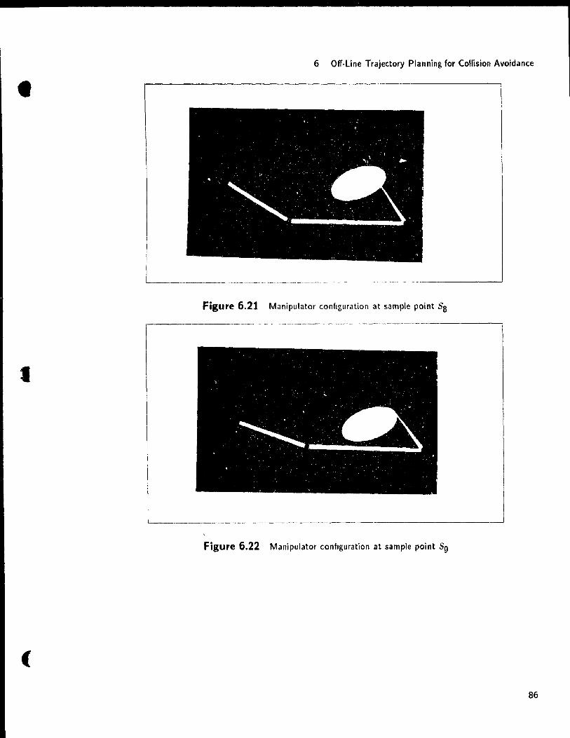
6 Off-Une Trajectory Planning for Collision Avoidance
L ______________________________ --_ - __________________ --l
Figure 6.21 Manipulator configuration at sample point S8
,------------- - - - -------- - ------ ------------------,
1
L-____________________ _
Figure 6.22 Manipulator configuration at sample point 89
(
86
Chapter 7 Conclusions
The inverse kinematics of redundant manipulators was studied in this thesls
From the point of view of devlsmg efficient algonthms for on-Ilne and off-Ime traJectory
planning
The eXistence of closed-form kmematlC Inversions for seven-axis. orthogonal.
wrist-partltioned manipulators. whlle mlnimizing an objective function of the joint angles
was mvestlgated ln the first chapter. but It was found that. though the flrst two Jomt angles
of the simple redundant arm archltec.ture can be determmed ln closed-form. the evaluation of
the la st two Joints of the arm requHed the solution of a 2-dlmenslonal optimizatlOn problem.
whlch on bemg solved symbollcally produced elther a system of equatlons that could be
dl-condltloned. or very hlgh-ordered polynomÎ<lls. the roots of whlch could be determined
only numencally However. It was demonstrated by an example that If the 2-dlmenslOnal
constrained optlmlzatlon problem IS solved numencally. then the resultmg hybnd algorithm
IS a very efficient means of performing the mverse kmematics of the mampulator under
study.
ln the fourth chapter a resolved-rate control scheme was presented for the
kinematic inverSion of redundant manipulators. The general scheme using the dlsplacement
Jacobian was modlfied and made computatlOnally efficient by formulatmg it in terms of the
veloclty Jacoblan along wlth the modifled vector of Lagrange multipliers It was shown
that the non-conservative effect is ehmmated in any case. An example was included to
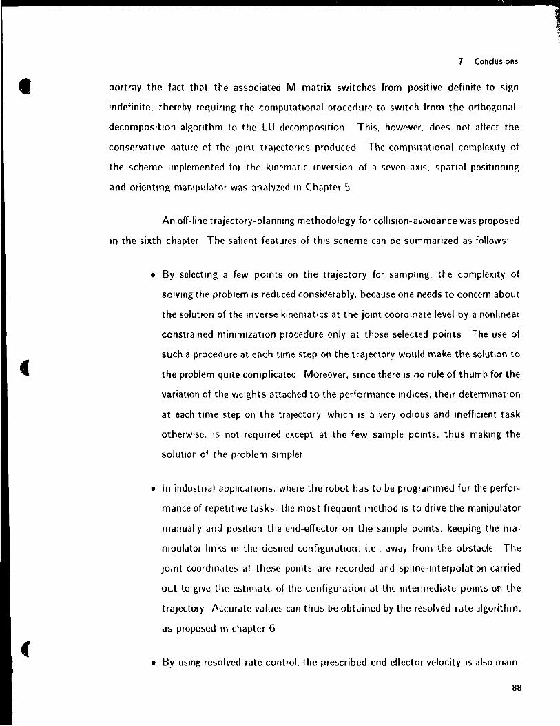
c
(
7 Conclusions
portray the fa ct that the associated M matrix switches from positive definite to sign
indefinite. thereby requinng the computatlonal procedure to sWltch from the orthogonal
decompositlon algonthm to the LU decomposltion This. however. does not affect the
conservatlve nature of the JOint traJectones produced The computatlonal comple)\lty of
the scheme Implemented for the krnematlc Inversion of a seven-axls. spatial position mg
and orientmg manlpulator was analyzed m Chapter ~
An off-line trajectory-plannlllg methodology for collislon-avOidance was proposed
ln the sixth chapter The sallent features of thls scheme can be summarized as follows'
• By select mg a few pOints on the trajectory for samplrng. the complexlty of
solvlllg the problem 15 reduced considerably. because one needs to concern about
the solution of the Inverse klllematics at the jOint coordmate level by a nonlmear
constramed minlmlzatlon procedure only at those selected points The use of
such a procedure at each tlme step on the trajectory would make the solution to
the problem qUlte complicated Moreover. smce there IS no rule of thumb for the
variation of the welghts attached to the performance mdlces. thelr determmatlOn
at each tlme step on the traJectory. whlCh IS a very odlous and mefflclent task
otherwise. 15 not requlred e)\cept at the few sam pie pomts. thus makmg the
solution of the problem slmpler
• In industnal applications. where the robot has to be programmed for the perfor
mance of repetltlve tasks. the most frequent method IS to drive the manipulator
manually and position the end-effector on the sample pOints. keeping the ma
nlpulator links ln the deslred configuration. i.e. away from the obstacle The
jOint coordlnates (lt these pOints are recorded and spline-interpolatIOn carried
out to glve the estlmate of the configuration at the Intermediate pomts on the
traJectory Accurate values can thus be obtained by the resolved-rate algorithm.
as proposed ln chapter 6
• By uSlng resolved-rate control. the prescribed end-effector velocity is also marn-
88
..
7.
tained. Thus. trom an industnal point of view. this scheme apparently has
the practicallty and simpliclty of an ofT-llne procedure of tracking a trajectory
using the teach mode. and yet has the accuracy afTorded by a software-based
procedure for the solutIOn of the inverse kmematlc problem
7.1 Suggestions for Future Research
An algorithrn can be derived starting from the resolved-rate control scherne of
Chapter 4. which will be !inear ln the Joint accelerations and the double derivative of the
Lagrange m'Jltlphers with respect ta tlme .
89
(
(
References
References
Anderson (1987) Inverse Kmematics of Robot Manipulators. In the Presence of Smgular
ities and RedundanCles. Masters Thesls. Department of Met hanlcal Englneenng. MeGill
Unrverslty. Montreal. Canada
Anüerson. K and Angeles. J (1987) "The kmematlc mverslOn d redundant manlpulators
ln the presence of redundancles". T 0 appear ln The Int Journal of Robotles Research
Angeles j (1985) "On the numencal solution of the Inverse Klnematlc problem". The Int
J of Robot/cs Re5 Vol 4, No 2. pp 21-37
Angeles J (1988) " Isotropy Criteria ln the Kmematlc DeSign and Control of Redundant
Mampulators", NATO Advanced Research Workshop, Robots w/th F?edundancy. Design,
Sensmg and Control, Spnnger-Verlag, ln press
Angeles J (1989) Robotlc Mechamcal Systems. An Introduction. McRCIM-Department of
Mechanlcal Engineering, McGili Ulllverslty, Montreal. Canada
Angeles J , Anderson K and Gosselln C (1987) "An orthogonal-decomposltion algorithm for
constralned least-square optlmlzatlon" . Proc, 13th ASME DeSign AutomatIOn Conference.
Boston, Sept 27-30, pp, 215-220,
Angeles, J , HabIb, M and L6pez-CaJun. C (1988) "EffIcient algorithms for the kmematlc
Inversion of redundant robot manlpulators". InternatIOnal J Robot/cs and AutomatIOn. Vol
3. No. 1. pp 106-116
Angeles, J and Lôpez-CaJLm. C (1988) "The dextenty mdex of seriai-type robotlc manip
ulators". ASME Trends and Development ln Meehamsms. Machines and RobotlCs. Sept
24-28. Klsslmmee, Flonda, Vol 3, pp 79-84
Angeles j, and Ma Ou (1989) "QUADMIN An Integrated Package for Constramed Nonlm
ear Least-Square Problems". Department Of Mechamcal Engmeermg and Robotlc Systems
Mechamcal Laboratory- MeRC/M. MeG'" Umvers/ty. Montreal. Quebec. Canada
Angeles. J, and ROJas. A (1987) "Malllpulator inverse kmematics via condltlon-number
mimmizatlon and continuation". Internat/onal Journal of Robotics and Automation. Vol. 2. No 2. pp, 61-69
Bailheul J, (1985) "Kmematic programming alternatives for redundant manipulators" . Proc,
IEEE Conf. on Robotics and Automation .. St. Louis. pp. 722-728,
90
1
References
Ballieul J. (1986) .. Avoidmg obstacles and resolving kinematic redundancies" Proc IEEE
Conf Robottcs and Automation San Fransisco. pp 1698-1704
Baker. D Rand Wampler. ( W (1987) "Some tacts concernmg the Inverse kmematlcs of
redundant manlpulators". Proc 1987 IEEE Int Conf Robottcs and AutomatIOn. Rayleigh.
Ne. pp 604-609
Benatl M . Morasso P . Tagllasco V (1982) " The Inverse kmematic problem of anthropo
morphlc mampulator arms" Trans ASME J Dyn. 5yst. Meas .. and Control. Vol. 104.
pp 110-113
Brooks R A (1983) "Plannmg collision-free motions for plck-and-place operations" Int.
Journal of Robottes Research Vol 2. No 4. pp 19-44
(hang P (1986). "A closed-form solution for the control of mampulators wlth kmematlc
redundancy". Proc IEEE Int Conf Robottcs and Automation. pp 1-14
Dubey R V. Euler J A. and Babcock S M (1988). "An effiCient gradient projection
optimlzatlon scheme for a seven-degree-of-freedom redllndant robot wlth sphencal wrists".
IEEE Int Conf on Robottes and AutomatIOn. Phlled~lphla. Vol 1. pp 28-36
Fisher W D. (1984) The kmematlc control of robot mampulatofs wtth fedundancy. Ph.D
Dissertation. Electncal Eng. Dept. Purdue University
Forsythe G E and Moler (B (1967) Computer Solutton of Linear Algebratc Systems.
Englewood (ltffs New Jersey. P,entlce Hall
Freund E (1977) " Path control for a redundant type of tndustnal robot" Proc 7th Int
Symp Industr Robots pp 107-114
Goldenberg A A Benhablb B Fenton R G (1985) "A complete generallzed solution to the
Inverse klnematlCs of robots". IEEE Journal of Robotics and Automatton. Vol. RA-l, No.
1 pp. 14-20
Golub G H and Van Loan ( (1983). Matrtx Computations. Baltimore The Johns
Hopkins University Press.
Hartenberg S. and Denavit J. (1964) Kmematic synthests of Imkages. McGraw-HIIi Book
Co .. New York
Hayward V (1988) "An anéllysis of redundant manipulators from several view-pomts".
NATO Advanced Research Workshop. Robots with Redundancy. Design. 5ensing and Con
trol. Springer-Verlag. In press.
91
,
«
References
Hollerbach J M and Suh K C (1987) "Redundancy resolutlon of manipulators through
torque optlmlzatlon", IEEE Journal of Robot/cs and AutomatIOn Vol RA-3. No 4. pp
308-316
Kazerounlan K (1987). "OptImal manipulatIOn of Redundant Robots" Int Jou",al for
Robot/cs and Automation. Vol 2. no 2. pp 54-60
Khatlb 0 and Le MaItre J F 11978) "DynamlC control of mampulators t')peratmg ln a
complex envlronment" Proc 3rd Int. C/SM-IFToMM Symp pp 267-282
Klréanskl M and Vukobratovlé M (1986) . Contribution to control of redundant manlpu
lators ln an envlronment wlth obstacles" Int Journal of Robotlcs Research VoiS. No 4
pp 112--119
Klein CA (1984) "Use of redundancy ln the deSign of robotlc systems" 2nd !nt Symp
on Robot/cs Research. Kyoto. Japan. pp 58--65
Klein ( A and Huang C (1983). "Revlew of the pseudOinverse control for use wlth
kmematlcally redundant mallipulators ". IEEE Trans Systems. Man and Cybernet/cs. Vol
SMC-13. No 3 pp 245-250.
Klem C A and Kee K (1989). "The nature of drIft ln pseudomverse control of kmematlcally
redundant manlpulators". IEEE Trans on Robot/cs and AutomatIOn. Vol. 5. No. 2. pp
231-234
L.légeols A (1975) .. Commande des systémes meéalllques articulés" RAIRO Séfle Au
tomatIque
LIégeOIS A 11983) "AutomatlC supervisory c.ontrol of the confIguratIon and behavlor of
multlbody mechanlsms" IEEE Trans on System. Man and Cybernet/cs Vol SMC-13. pp
245-250
Loeft l A and Sonl A H (1975) "An algorithm for computer gUidance of a manlpulator
ln between obstacles" ASME J Engmeermg (or Industry Series B. Vol (97). No 3 pp
836-842
Lozano-Pérez T (1983) "Spatial planning A configuration space approach" IEEE Trans
on Computers Vol c-32. No 2 pp 108-120
Luh J Y S and Gu L Y (1985) "Industnal robots with seven JOints". IEEE Conf Robot/cs
and AutomatIOn St LoUIS pp. 1010-1015.
MacieJewskl. A. A. and Klein. C A (1985) "Obstacle avoidance for kmematically redundant
manlpulators in dynamlcally varying envlronments". The Internat/onal Journal of Robotics
Research. Vol 4. No. 3. pp. 109-117
92

-References
Mangasarian 0 L (1972) "Techniques of optimization" Trans. ASME J. Eng. for Ind
93. pp 303-309
Nakamura Y . Hanatusa H . Yoshikawa T (1987) "Task-Prronty based redundancy control
of robot manlpulators". The Int Journal of Robot/cs Research. Vol 6 No 2. pp 3-15
Pleper D (1968) The kmemdt/cs of 1T1cIf1I{Julators under computer control. Ph D Thesls.
Dept of Computer SCIence. 5tanford UnIversIty
Pnmrose E J F (1986) "On thr Input-output equatlon of thE' general 7R mechamsm".
Mechamsm and Machme Theory. Vol 21. No 6. pp 509-510
Salisbury. J K and Crd\?,. J J (1982) "ArtlCulated hand~ torre and kinematlc Issues".
The International Journal of Robotl(~ Research. Vol 1. No 1. pp 4 -17
SClavlCCo Land 51clllano B (1988) "A solutIon algonthm to the Inverse kmematlc problem
for redundant mantpulators" IEEE Journal of Robot/cs and AutomatIOn Vol 4. No 4 pp
403-410
Stant~lé M M and Pennock G R (1985) "A non degenerate ktnematlc solution of a seven
JOlnted robot mampulator". The Int JOIlff1<11 of Robot/cc, Research. Vol 4. No 2. pp
10-20
Whitney 0 (1972) "The mathematlCs of co-ordmated control of prosthetrc arms and ma
nlpulators" ASME J Dynamlc System. Measure. Control pp 303 309
WillIams 0 R (1989) Kmemat/cs and deSign of robatte ma",pulators w/th comp/ex architec
tures. Masters Thesls. Department of Mechanlcal Engineering. McGl1I University. Montreal.
Canada
Yahsl 0 Sand Ozgoren K (1984) "Minimal JOint MotIon Optlnllzatlon of Manlpulators
wlth Extra Degrees of Freedom ... Mechamsms and MdChtne Theory Vol 19. No 3. pp
325-330
Yoshikawa T (1983) "Analysis and control of robot mampulators wlth redundancy" Proc
lst /nt. Symp on Robotics Research pp. 735--747
Yoshlkawa. T (1985) "Mampulablltty of robotlc mechamsms". The International Journal
of Robotics Research. Vol 4. No 2. pp 3-9
93

t
c
Appendix A
Appendix A.
Here. the steps used in the derivation of equations in chapter 3 are given.
A.t Solution for 02
On rearrangmg eq (3.16) we obtain
Now. on wntlng ail the rotation matrices and the vectors in terms of the respective jomt
angles. the following equatlon IS derived
From thls vector equatlOn. two scalar equations can be obtamed as
a4cos(83 + (4) + G3 cos 03 + a2 = ~cos02 + 7] sm02
04 sm (° 3 + (4) + 03 sin03 = 17Cos 02 -- ~sm02
The result obtained on solving the aforementloned equatlOns slmultaneously for sin fh and
c0502 i5 given ln eq5.(3.17 & 3.1&) respectlvely
A.2 Oerivation of the constraint equation
The constramt equatlon IS obtamed simply by addmg the squares of both the
sides of eqs (3.17 & 3.18) Thus. the followmg IS obtatned
and
L =a/ + a32 + 02
2 + 2a3a4 cos 04 + 2a2a3 cos 03 + 2a2a4 coS(03 + (4)
R =~2 + i}2
L=R
where. Land R denote the sum of the squares of the left-hand and the right-hand si des of
eqs.(3.17 & 3.18). respecttvely. ThiS equation can now be condensed ioto the form given
in eq.(3.25). which IS the constraint equatlon
94
Appendix B
Appendix B.
The followmg are the coefficients of the 24th order polynomial. which were
derrved by substltutrng '3 = ( 1114: \ 1(2/~ 4(/~'+(,"~)(Ft~+ .J)]'12(1·,'+ G/ l)] m
eq (11). Note that ail the derrvatlons were performed usrng the symbollc computation
5>oftware, 'MACSYMA' The 'FORTRAN' command of MACSYMA was used then ta con-
vert the symbolrc notation rnto fortran format Thereafter. thls format was transformed
mto Tex. as It appears now. by maklng some global changes ta the fortran flle usrng the
system's edltor
Al =lm - Tl
.42 =/2 .. T2
.'15 =(2,lk + 2h)m + 2il - T5
.46 =2gm + (2]k + 211)1 T6
.17 =2f1l/ .... 2y' r7
A8 =2f'T1i + 2fl + 12 Ta
Ag =2drn + 2e1 + 21Jk + 2/11 Tg
AlO =20n + 2dl + /1.- 2 + 2h.Jk + 2g1 + 112_ TlO
A11 =2hrn + 2rl -+ 2fl.lk + 2fl + 2qh rU
A12 =2am + 2b' + 2f.lJ..' + 2Cl + 2fh + r/- T12
AB =2(1/ + 2eJk + 2dl + 2('11 + 2fq T13
.4 14 =2~lk + 2('1 + 2dh + 2ey + f2 T14
.4 15 =2cJk + 2bl + 2ch + 2dy + 2e f - T15
A16 =2bJk + 2a! + 2hh + 2cy + 2df + e2 - T16
A17 =2ajk + 2ah + 2bg + 2ef + 2de - TH
(B.l )
(B.2)
(B.3)
(B.4)
(B.5)
(B.6)
(B.7)
(B.8)
(B.9)
(B.I0)
(B.11 )
(B.12)
(B.13)
(B.14)
(B.15)
(B.16)
(B.17)
(B.18)
95
where
c
AlS =2ag + 2bf + 2ce + d2 - r1S
Al9 =2af + 2be + 2cd -- rl9
A20 =2ae + 2bd + ('2 - T20
A21 =2ad + 2bc - r21
An =2{/(' + h2 - r22
1123 =2ab T23
A24 =a 2 - r24
a = - 16FC3 L
b =16G4 h' + 16F2(;2Q -- 16FC3 P -- 8C3 HAl + 24FC2 H K
(' ={16F2(.'2 - 16(4)T - 8(;3 H R + 24F(;2 II N+
(16G3.1+8G2II2 48E1'(;2)L
d =16C4 Z 16F(,'3 X + 16F2C;2\" + (24FC2 - BC3) Il U +
Appendix B
(B.19)
(B.20)
(8.21 )
(B.22)
(B.23)
(B.24)
(8.25)
(B.26)
(B.27)
( 8.28)
64EG35' + (32FC;2 J - 32FC Jl2 + 32EF2G)Q + (--16C3 J + SC2 H2
--48EFC;2)}, 24EC2H.T\1 + (24G 2H.J 8G'1l3 + 48EFCH)K (8.29)
e = - s(;311)" + 24FG2 /l\f + (32F(;2,/ - 32FGl/ 2
64E(,,] + 32EF2(,')T 241;G 2 JI H + (24C 2 H.J 8C1l 3 + 48EFCll)X
f =64EG 3 Z + ( 16(,,3.J + au2 Jl2 - 481~' F(2)X + (32FG2.1-
321'(; H2 + 32E F2C) \ + \24(,,2 JJ.J - BG1l 3 + (48E FG - 24EC2)JJ)U
+ 96E2(,'2.c.,' + [16C2.1 2 + (64EFG 32C1l 2)J + 81/4 -- 32EFl/2+
16E2 F2JQ + ( 48EC2 J + 16EG1l 2 - 48E2 FC)? + 24FC2 lfO-
9 = - 24EG2 H}" + (24C 211 J -- BGlf 3 + 48EFGlI)W +
(16C2.12 + (64EFC - 32CH 2)J + 8H 4 - 32EFH 2 -- 96E2C2+
16E2 p2JT - 24E2CH R + (48ECH J - 8Elf 3 + 24E2 F H)N + [(16C3
( 8.30)
( B.31)
96
and
Appendix B
- 48E2G)J + (8E 2 -- 8G2)11 2 + 48EFG2 -- 16E3 F]L (B,32)
h =96E2C;2 Z + ( 48/-X,,2.1 + 16EG}[2 48E2 FG).\" + 116G2.1 2
+ (64f.;F(,' 32GJJ 2).J + 8JJ4 32HFI/ 2 + 16/~,2F2]r + 148EGl/.1
8/;1/3 + (24J,2 r 24}~,2(,')I/]I' + 64F 3U,I.; + [32E(,'.j2 + (32f.l,2 F
- 32H 1/2 )./](( + ( 48 }:,'] G.I + 8/-,,21/2 16/j,3 F) J' + (24(;2/1./ 8G 11 3
+48EFGII)O 8E 3J1.\1+24E 211.Jh 24f,'U2 J11 (B.33)
i = -- 24E2CJI}' + (481,'(;1/./ 81,'1/3 + 24/j'2 F I/)W+
132f.l'G.l2 + (32};2 F 32/-,'11 2).1 64/~jG]T 8E3 H R + 24E2Jl J N +
1(48EG2 16]j'3).1 16EGI/ 2 + 481.;2 FU]L (8.34)
j =64E3C; Z + ( 481,>,2(,'.1 + 8E2,,'} 16E3 F).\" +
132EG.l2 + (32/j'2 F 32EJJ 2).I]\' + (24/,,2 H J - 8E311)fT + 16E4 S +
16E2.J2Q - 16E~J P +- (48E'G JI.I 8E /{3 + 24E 2 F iJ)O - E 2GIll (B.35)
k = - 8E311}' + 24E2 JJ.lll' + (16/.;2.1 2 -- 16E4 ),/,+
(48E~ GJ - 8E2 H2 + 161, l P) L
1 =16E4Z 16E3JX + 16B2J'}\, + 24E2lJ.J() 8E3 Hl
nt =16E 3JL
Tl = - 8EJa.:,
r2 =( -4GJ + H2 -- 4EP)ç2 -- 8EeJç - 4EJa 2
r3 =[( -8CJ + 2H 2 -- 8EF)a - BEoJh -- 8EeJa
r4 = - 4FG.:,2 + 1(- 8Gg - 8Eu)J + (2lJ 2 8EF)e]<.+
(--4GJ + H 2 -- 4EF)o2 8EoJa -- 4Er/J
r5 =(-8FGa + (-8Go 8Ep)J + (2l/ 2 8EF)o]ç+
(( -BGe - BEv)J + (2H 2 -- BEF)eJa -- 8EoeJ
T6 =[( -BCu - 8EK:)J - 8FCe + 2vH 2 - BEFv]ç - 4PGa2+
(B.36)
(B.37)
(B.38)
(B.39)
(B.40)
(B.41)
(B.42)
(B.43)
(B.44)
Q7
(
(
Appendix B
[(-8Co -- 8E/-L)J + (2H 2 - SEF)oJo + (-4Ce2 - SEve - 4Eo2)J
+ (//2 - 4EF)ri
r7 =[( -81lG - 81 E).J - SFGo + 21lH2 - BEFIl)ç + [( -SCv - BEK).J
- 8FG(J + 2vH 2 - 8EFv1a + [(-8Go - SEIl)e 8Evo).J
(8.45)
+ (2H2
- 8EF)oQ (8.46)
r8 =(( -8KG - 8d E')J + 21' Jl2 - SFGv - SEI'I:FJ.:; + 1(-- 8/-L C - StE)J
-- 8FGo -r 2p H 2 -- BE FILla + [( -- 8Gv -- BEK)e - 4G02 - 8EIlo
- 4El12).! 4FGri + (2vfI 2 - 8EFv){! + (H 2 .... 4EF)02 (8.47)
r9 =[( -8LG - SoE)J + 21H 2 8FJLG - 8LEF] ... + [( -81'1:G - 819E)J
+ 2K1I2 -- 8FGI! -- Bl'.t'I{ F]a + (( 8/-LG - 81 l'J') (! + (-8Gv - SEK)O
- 8EJLvIJ + (- 8FGo + 2fJ.JJ2 - 8EFIl)e + (2vH 2 - 8EFlI)0 (8.48)
T10 =[(- 8dC' - 8,E)] + 2{}H 2 - 8Ki"G - 819EF1.::: + I(-S/oC - 86E)J
+ 2LH2
- 8FIlG -- 8d,'FJa + ((- 8KG - 8vE)(! + ( -8/-LG - SLE)o
- 4G1I2 -- 8EKV -- 4EIL2]J + (21'1:11 2 - 8FGv -- 8EKF)e--
4FC02 + (211 H 2 -. BE FIL)o + v 2 H 2 - 4E F1I 2 (8.49)
r11 =(-8t5GJ + 20/1 2 - 8IFG·- 8bEF)" + ((---8t9G - 8,E)J
+ 219H 2 8KFG 81JEF]a + [( - 8lG - 8bE)(! + (-8KG - 819E)0
+ (-8JLG - 8IE)lJ- 8EKJL).J + (21H 2 - 8Fp(J' 8/EF)e+
(2KH 2 - BFGv - 8EKF)o + 21WH2 - 8EFju./ (8.50)
T12 =(-8,GJ + 2~r/12 - 8,JFG - B,EF).:. + (--8bC') + 2bH 2 - SLFG
- 86EF)a + (( ·8lJ(; - 8~iE){! + ( -8LG·- Si>E)o + (-8KG - 819E)v
- 4/-L2C -- 8LEIl - 4EK2)J + (21H1 2 - 81'1:FG -- 8{}EF)e
+ (2tI1 2 - 8F J..lG - 8lEF)0 + (2KV + JL2)1l2 -- 4FGl/ - 8EI'I:Fv-
4EF,,/ (8.51)
TB = - 8bFGç + (-8,GJ + 2,H2 - 8iJFC - aïEF)a
+ [- 8bGe + (-8dC - 8,E)0 + (-8LG - 88E)v - S"'IlG - 8dEIl
98

Appendix B
- 8LEK]J + (26H 2 - 8LFG - 8hEF)e + (2dH 2 - 8/'i,FG - 8dEF)o
+ (2ll/ + 21\:jJ) H2 + (-8Ff.1G -- 8LEF)v - 8EKFf.1 (8.52)
T14 = -- 8,FG.., - 86FGo + [-B,G2 -- BbGo + (--BdC - 8,E)v
+ (--B/jJ -- 4K2)G 8bEjJ - 8dL'K - 4,2E ].J + (2,1l2
- 8vFG - 8~tEF){! + (2fJlf 2 8, FG 86EF)o + (2dv
+ 2lf.1 + K2)JJ2 + (8KFG 8dEF)v 4Ft/G -- 8lEFIl - 4E/'i,2 F (B.53)
715 = - 8') FGo + [-- 8~,G() - 8b Gv + (- 8âJl - 8lK)G - 8')Ej.J--
86EK - 8dlE).l 8bFG{! + (2)1l2 BdFG B1EF)o
+ (26v + 2Jj.J + 2LK)1I 2 + (-8,FG - 86EF)v - BKFjJG-
8d J,' FI' -- 8t1:J'K F (B.54)
T16 =[-- B,Gv + (- BOjJ - 8tJK - 4t,2)G 8,EK + (-B6i -- 4d2)E]J
- 8~IFG{! - 86FGo + (2")'1/ + 26jJ + UiK + (2)1l2
+(--8dFG- B,'EF)v+(-BlFIl· 4K 2F)G-8liEFjJ+
(-- Bd EK - 4L2 E)F (B.55)
717 =[( --B11l - 86K - 8th)e; + (- B,l - 8bd)E]J
- 8, FGo + (211/ + 2br. + 219, )11 2 - Bb l'Gv
+ ( BvFtt 8,r.'F)(,' 8,[;FI' + ( 8/lEK - Bd/E)F
718 =[( -- 81 K - 8hL 41)2)C' + ( 8,t) 4b 2)l!,'].l + (2"'(K + 2[u + d2)H2
--8,FGv+[( 8th 4,2)1' 8hF'I]G+[( 8/l, 4t?2)E-
8~(E,.;:]F
T19 =[( --8)l - 86tJ)G 8-rbE]] + (2-(, + 2bd)JJ 2
+ [( -- 8hK 8d,)F - B,Fll]G + (- 8 Il - B617)EF
720 =[( -8)19 - 46 2)G - 4l E]J + (2')d + 1/)11 2 +
(B')K 8hL - 41?2)FG + (- B)d - 4fJ 2)EF
T21 = - B,liG.J + 2,611 2 + (--8~tl - 86tJ)FG - 8,liEF
T22 = - 41 2GJ +,2/i2 + (--8,t? -- 46 2)1'G - 4/EF
(8.56)
(B.57)
(B.58)
(B.59)
(B.60)
(B.61)
99
1
Also.
{
(
Appendix B
T23 = - 8"'1DFG
T24 = - 4"'12FG
"'1 =8C3 M -- 8FC2 K
D =8C3R -- 8FC2,V - 8G2HL
11 =(8C3
- 8F(2)l' + 16FCHQ - 8C2HP + 24EC2M+
(-8G2J + 8GH2 --16EFC)K
L =8C3y -- 8FG2W + 16FGHT + 24EC2 R + (-8C2J + 8GH2-
16EFG)lY - 16ECH L
K. = - 8G2H X + 16FGH~' + (-8C2 J + 8GH2 + 24EC2 -- 16EFG)U+
(16GHJ -- 8H 3 + 16EFll)Q - 16EGH P -- 8FG20 + 24E2GM+
(-16EGJ + 8E1I2 - 8E2F)K + 8G31
J1 =24EC2}, + (-8G2 J + 8GH2 - 16EFG)W + (16GH J - 8H3+
16EF H)T -r 24E2CR + (-16ECJ + 8E H 2 - 8E/ F)N +
(B.62)
(B.63)
(B.64)
(B.65)
(B.66)
(8.67)
(8.68)
(8C2
- BE2) II L (B.69)
v = - 16EGJJ X + (16C II J -- 8JJ 3 + 16EF H)~r + (--16EGJ + 8EH2+
24E2C - BE 2F)l' + 16ERJQ- BE2lJp + (-8C2J + 8GH2
- 16EFG)O + BE3A1 - 8E2 J K + 24EG21 (B.70)
o =24E2C}' + (-16EGJ + 8ER2 - 8E2 F)J'V + 16EH JT + 8E3 R-
8E2JX+16EGHL (B.71)
{! = -- 8E2 H X + 16ER JV + (8E 3 - 8E2 J)U + (-16EGJ + 8EH2
- 8E2 F)O + 24E2C 1
u =8E3y - 8E2 Jl-V + BE2 H L
ç =8E31 - BE2JO
(B.72)
(B.73)
(B.74)
100
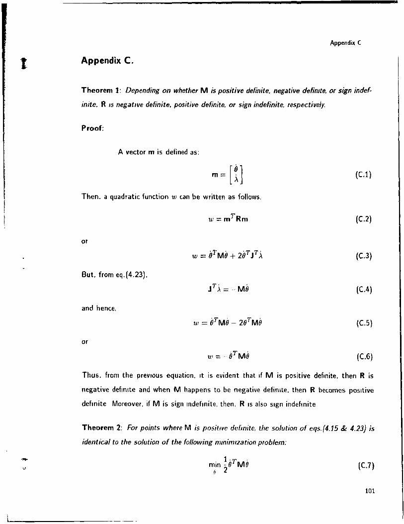
t
'.>
Appendix C
Appendix C.
Theorem 1: Depending on whether M is positive definite. negative defimte, or sign indef~
inite. R IS negatlve de fin i te, positive definite, or sign indefinite, respective/y.
Proof:
A vector m is defined as:
m== [t] Then, a quadratic function w can be written as follows.
or
But, from eq.(4.23),
and hence,
or 'r .
w == -0 MO
(C.l )
(C.2)
(C.3)
(C.4)
(C.5)
(C.6)
Thus, trom the prevlous equation, It is evident that If M is positive definite, then R is
negative defmlte and when M happens ta be negative defimte. then R becomes positive
defmite Moreover. if M is sign rndefmite. then. R IS also sign indefmite
Theorem 2: For points where M is positive dermite. the solution of eqs.(4.15 & 4.23) is
identical to the solution of the (ollowing mmimlzat;on problem:
(C.7)
101
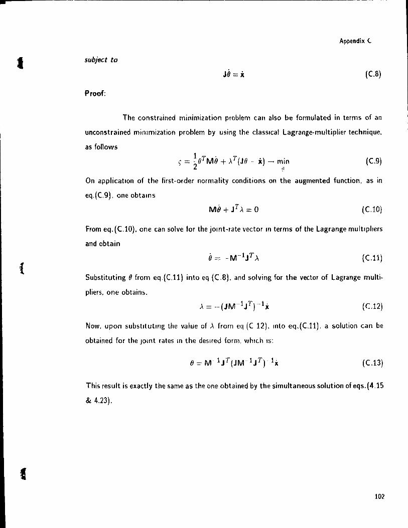
•
(
Appendix t
5ubject to
JO = x (C.S)
Proof:
The constrained minimization problem can also be formulated in terms of an
unconstrained mimmization problem by using the classlcal Lagrange-multiplier technique.
as follows
(C.9)
On applicatIon of the first-order normality conditions on the augmented function. as ln
eq.(C.9). one obtarns
(C.l0)
From eq.(C.l0). one can solve for the jOint-rate vector m terms of the Lagrange multlplrers
and obtain
(C.11)
Substituting 0 from eq.(C.11) into eq (C8). and solving for the vector of Lagrange multi
pliers. one obtains.
(C.12)
Now. upon substltutrng the value of À from eq (C 12). mto eq.(C.11). a solution can be
obtained for the jOint rates ln the deslred form, whf(.h IS:
(C.13)
This result is exactly the same as the one obtained by the simultaneous solution of eqs. (4.15
& 4.23).
102

1
Appendix D
Appendix D.
A linear constrained minimization problem can be given in the form:
subject to
where
mmz x
ex = d
1 T z = -- (Ax - b) W(Ax - b) 2
(0.1 )
(0.2)
(0.3)
A being an m À n matrix. while x, band d are n. ln and p-dlmensional vectors respectively.
W is nothing but a m x m. positlve-semldefmite weighting matrix Next. the flrst-order
and the second-order conditions for a constramed mmlmlzation of z are derived. To this
end. an augmented functlon ç is formed as follows'
(0.4)
where ). is the p-dimensional vector of the Lagrange multipliers. The first-order normality
condition of the foregoing problem IS then.
(0.5)
which can be rewntten as
(0.6)
What eq (D 6) states IS that. at a statlonary pomt. there eXlsts a p-dlmensional vector ).
that verifies exactly the overdetermined !lnear system appeanng in eq.(D.6) This vector.
denoted by >'0. IS nothmg but the least-square approximation of eq.(D.6). i.e ..
(0.7)
and hence. the first-order normality condition states that the least-square error. eO. defined
below. vanishes at a stationary pOint. i.e ..
(0.8)
103
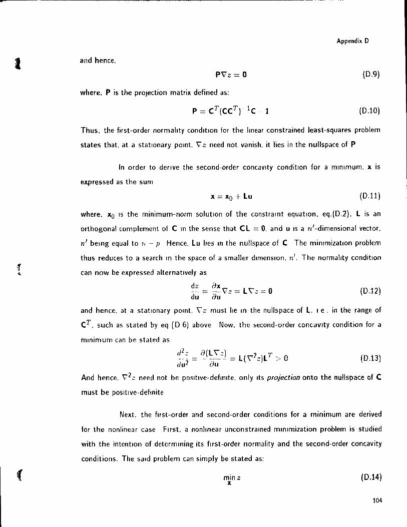
•
t
(
Appendix D
and hence,
PV'z = 0 (D.9)
where, P is the projection matrix defined as:
(D.tO)
Thus. the first-order normahty condition for the "near constrained least-squares problem
states that, at a statlonary pOint. v z need not vanish, it lies in the nullspace of P
ln order to denve the second-order concavlty conditIon for a minImUm, x is
expressed as the sum
x = Xo + Lu (0.11)
where. Xo IS the mlnlmum-norm solution of the constramt equatlon. eq.(D.2). L is an
orthogonal complement of C ln the sense that CL = O. and u IS a n'-dimensional vector,
n' bemg equal to 1/ - P Hence. Lu Iles m the nullspace of C The minlmizatlon problem
thus reduces to a search ln the space of a smaller dImenSIon, n'. The normallty conditIOn
can now be expressed alternatlvely as
dz
du
ax -V'z=L~z=O au (0.12)
and hence. at a statlonary pOInt. '\::: must Ile ln the nullspace of L,le. in the range of
CT, such as stated by eq (D 6) above Now, the second-order concavlty condition for a
mmimum can be stated as
d2:: a( L '\ ::) 2 \ T_ --- = -- ----- = L(\' zJL ;> 0 du2 au
(0.13)
And hence. \72::: need not be posltlve-defmlte. only Its projection onto the nullspace of C
must be posltlve-defmite
Next. the flrst-order and second-order conditions for a minimum are derived
for the nonlinear case Flrst, a nonhnear unconstralOed mlnlmization problem is studied
with the intention of determming its flrst-order normality and the second-order concavity
conditions. The sald problem can simply be stated as:
minz x
(D.14)
104
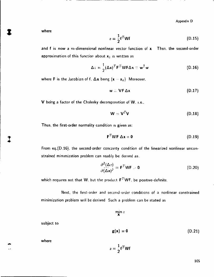
l
Appendix 0
where 1
z = -fTWf (0.15) 2
and f is now a m-dimensional nonlinear vector function of x Then. the second-order
approximation of this function about xI: IS wntten as
(0.16)
where F is the Jacobian of f. {j"x bemg (x . xd Moreover.
w ~-= VFô.x (0.17)
V being a factor of the Cholesky decomposltion of W. I.e ..
(0.18)
Thus. the first-order normality condition IS given as:
(0.19)
From eq.(0.16). the second-order concavlty condition of the linearized nonlinear uncon
strained minlmization problem can readlly be denved as.
(0.20)
which reqUires not that W. but the product FTWf. be posltlve-defmite.
Next. the flrst-order and second-order rondltlons of a nonlinear constrained
minimizatÎon problem will be derived Such a problem can be stated as
subject to
where
mmz x
g(x) = 0 (0.21)
105
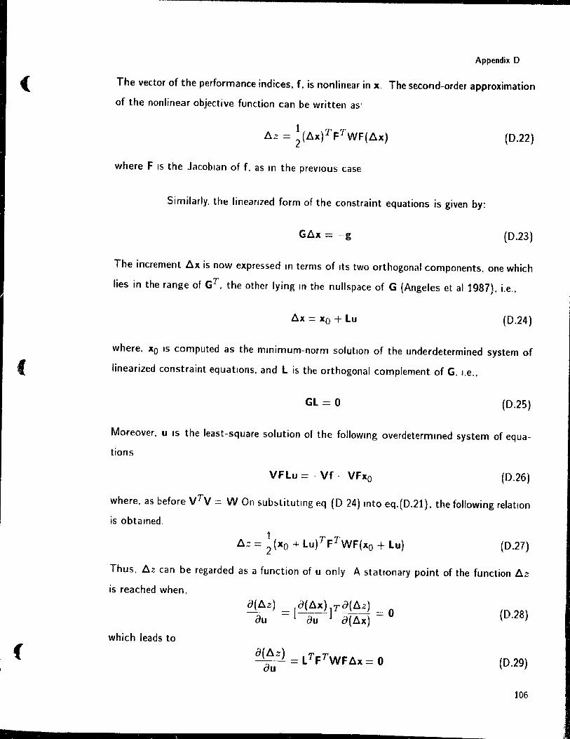
(
(
{
Appendix D
The vector of the performance indices. f. is nOrllinear in x. The second-order approximation
of the nonlinear objective function can be written as'
(0.22)
where F IS the Jacoblan of f. as ln the prevlous case
Similarly. the lineanzed form of the constraint equations is given by:
Gl:!.x = --g (0.23)
The increment tu is now expressed ln terms of Its two orthogonal components. one which
lies in the range of GT. the other Iying ln the nullspace of G (Angeles et al 1987). i.e ..
l:!.x = Xo + Lu (0.24 )
where. Xo IS computed as the mmimum-norm solution of the underdetermined system of
linearized constraint equatlons. and L is the orthogonal complement of G. I.e ..
GL = 0 (0.25)
Moreover. u IS the least-square solution of the followlng overdetermmed system of equa-
tions
VFLu = -Vf - VFxo (0.26)
where. as before VTV = WOn substitutmg eq (0 24) lOto eq.(0.21). the following relation
is obta med.
(0.27)
Thus. llz can be regarded as a function of U only A statlonary point of the function /j"z
is reached when.
a(/j"z) = [a(l:!.x) ]Ta(l:!.Z) = 0 au au a(l:!.x) (D.28)
which leads to
(0.29)
106
1
----------------------------------
Appendix D
Equation (0.29) can also be written as:
LTv(Az) = 0 (0.30)
i.e .. at a statlOnary pOint. v(f),z) Iles ln the nullspac.e of LT The second-order concavity
condition for the second-order approximation of 6.::: to be a minimum 15 as follows.
(0.31)
I.e .•
(0.32)
which can also be written as:
(0.33)
This condition is obvlously different from the minimum condition of the nonlinear uncon
strained mlnlmlzation problerr.. shown in eq (D 20). for eq.(D.33) requires that not \72z
itself. but its projection onto the null space of G. be posltlve-definlte
107
«
(
Appendix E
Appendix E.
E.l Derivations for aÀ/aiJ
Matrix A IS given as:
À == [èt (E.1)
where
(E.2)
and Wt -l is the angular velocity of the (1 - 1)st link. The partial derivative of the A with
respect to the Joint rates WIll result ln a thtrd-rank tensor aA/aO. Now. W 1 -1 can be
derived in terms of the Joint rates as:
. . Wz-l = 0lel + ... + 0t-l ez-l (E.3)
Therefore. è~ can also be written in the form'
(E.4)
Now. each vector component v1 ) of the third-rank tensor aÀ/aiJ will comprise of terms
derived as follows. __ ae!
VI] =-=- ail J
From eq. (E 4) it is apparent that v1) wIll be of the followlng form
{O. for 1 = 1. . . n and J == l, ... , n:
VtJ == eJ " ez ' for 1 = 2, . ,n and J == 1, ... z - 1.
The same can then be written in matrix form as:
0 0 0 0 el x e2 0 0 0 aA el x e3 e2 )t: e3 0 0
ao
el x en e2 x en e n-l X en 0
(E.S)
(E.6)
(E.7)
108
a
-,-
Appendix E
E.2 Derivation for aB / an
Matrix B takes on the form:
(E.8)
where
(E.9)
U1 is also defined as:
vector W i) bemg the three-dimensional (l. J) vector component of the third-order tensor
aB/BO
Vector el can be wntten as in eq (E.4). whereas. rI can be written ln the
followmg form'
i=1,2, .. ,no (r:.1 0)
On substituting .... ·1 from eq (E.3) mto eq (E.10). the following expression for ri IS obtamed'
;1 = (Olel + .. +Oez)' al + (Olel + .. . +Ol+1el+1) >,a1+1 +. +(Oel + .. +OTle r /) • a r,
(E.ll)
The third-rank tensor aB 1 (JO is then derived by evaluatlng the partial derivatlve of ui
wlth
respect to the Joint rates 0) For 1 = 1. .11 and J = 1. .1 1 one can obtam thls
partial denvatlve wlth the ald of eqs (E 4. E 9& E Il) ln the forlll
~~I '..: w l ) = (e, ' el) . fi + el > (e, ' fi) (E.12) J
which can be condensed further to glve
(E.13)
For l = 1, ... ,n and j = i, . .. , n. w 1) takes on the form:
(E.14)
109
li
(
(
(
Appendix E
When written in matrix form. the third-rank tensor as / an appears as:
as 80
el > (e2 x r2) el" (e3 x r3) e2 ), (e2 x r2) e2 x (e3 x r3)
. .. el x (en x rn ) 1
. " e2 x (en X rn )
en x (en )f rn)
(E.15)
110