AIAA 2002-4875 Simulation and Flight Control of an Aeroelastic...

AIAA 2002-4875Simulation and Flight Controlof an Aeroelastic Fixed WingMicro Aerial Vehicle

Martin R. Waszak and John B. DavidsonNASA Langley Research CenterHampton, VA 23681-2199

Peter G. IfjuUniversity of FloridaGainesville, Florida 32611-6250

AIAA Atmospheric Flight Mechanics Conference5–8 August 2002

Monterey, CA

For permission to copy or to republish, contact the copyright owner named on the first page.For AIAA-held copyright, write to AIAA Permissions Department,1801 Alexander Bell Drive, Suite 500, Reston, VA, 20191-4344.

1American Institute of Aeronautics and Astronautics

SIMULATION AND FLIGHT CONTROL OF AN AEROELASTIC FIXED WINGMICRO AERIAL VEHICLE

Martin R. Waszak* and John B. Davidson†

NASA Langley Research Center, Hampton, VirginiaPeter G. Ifju‡

University of Florida, Gainesville, Florida

Abstract

Micro aerial vehicles have been the subject of continued interest anddevelopment over the last several years. The majority of current vehicleconcepts rely on rigid f ixed wings or rotors. An alternate design based on anaeroelastic membrane wing has also been developed that exhibits desiredcharacteristics in f l ight test demonstrations, competition, and in prioraerodynamics studies. This paper presents a simulation model and anassessment of f l ight control characterist ics of the vehicle. Linear state spacemodels of the vehicle associated with typical tr immed level f l ight condit ionsand which are suitable for control system design are presented as wel l . Thesimulation is used as the basis for the design of a measurement based nonlineardynamic inversion control system and outer loop guidance system. Thevehicle/controller system i s the subject of ongoing investigations ofautonomous and collaborative control schemes. The results indicate that thedesign represents a good basis for further development of the micro aerialvehicle for autonomous and collaborative controls research.

Introduction

Micro aerial vehicles, or “MAVs”, are typicallydesignated as a class of aircraft with a maximumdimension of 6 inches that are capable of operating atspeeds of 25 mph or less.[1] Developments inminiaturized digital electronics, communications, andcomputer technologies and strong support by DARPAhave moved the prospect of very small autonomousflight vehicles from the realm of science fiction toscience fact. The goal is for these vehicles to provideinexpensive and expendable platforms for surveillanceand data collection in situations where larger vehiclesare not practical. For example, they can be used for

* Senior Research Engineer, Dynamics and ControlBranch. Senior Member AIAA.† Senior Research Engineer, Dynamics and ControlBranch. Senior Member AIAA.‡ Associate Professor, Department of Aerospace,Mechanics, and Engineering Sciences.

Copyright © 2002 by the American Institute ofAeronautics and Astronautics, Inc. No copyright isasserted in the United States under Title 17, U.S. Code.The U.S. Government has a royalty-free license toexercise all rights under the copyright claimed herein forGovernmental purposes. All other rights are reserved bythe copyright owner.

battlefield surveillance or mapping the extent ofchemical/radiation spills or viral outbreaks. Otherapplications include use in search and rescueoperations, traffic/news coverage, and crop or wildlifemonitoring. Many potential uses would requirecooperative and collaborative control capabilities sothat large numbers of MAVs could be used to cover alarge operational area. In these types of applicationsMAVs could be coordinated from a central basestation or used in collaborative swarms to collect andtransmit data.

The research and development required fordeveloping MAVs and related systems is technicallychallenging and requires a number of technologicaladvances that may benefit a broad range of aerospaceapplications. The development of a vehicle could alsofoster development of component technologies andhelp to support an emerging growth market for microaerial vehicles.

An aeroelastic fixed wing micro aerial vehicleconcept has been developed by a team at the Universityof Florida with a goal to design a vehicle that couldwin the ISSMO (International Society of Structuraland Multidisciplinary Optimization) Micro AerialVehicle Competition; a goal that has beenaccomplished each of the last four years.[2,3]

The vehicle exploits an innovative aeroelastic wingwith the ability to adapt to atmospheric disturbances


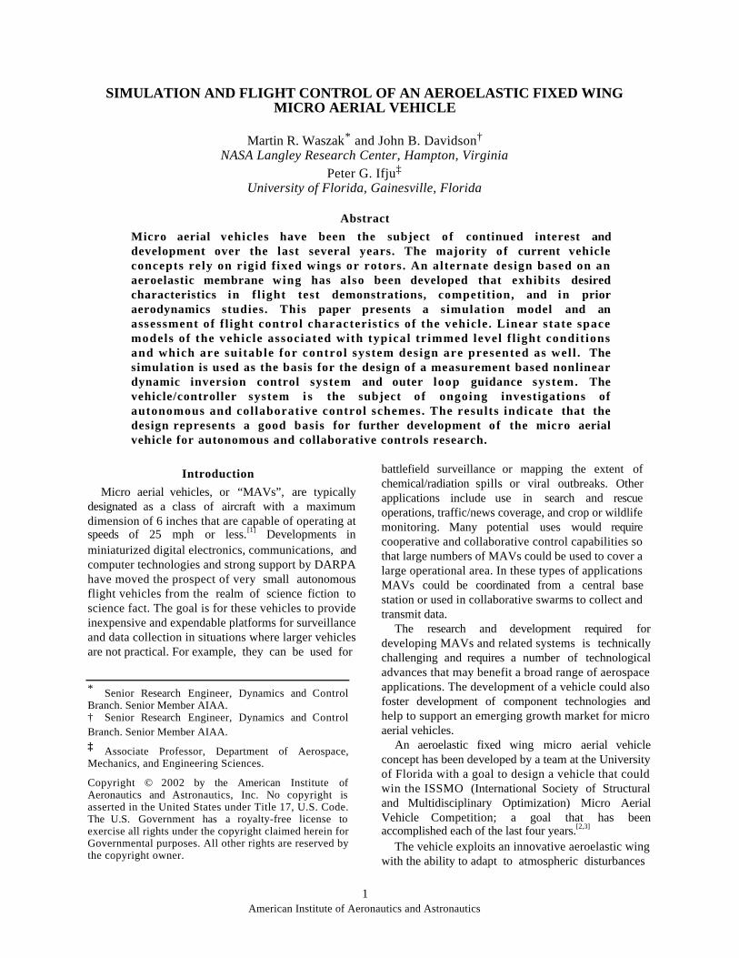
Figure 1 – photograph of Univ. of Florida MAV.

and provide smoother flight thereby providing a bettersurveillance platform and making the vehicle easier tofly. This is accomplished via a passive adaptivewashout mechanism.

The adaptive washout technique has been taken fromsailing vessels which use sail twist to greatly extendsthe wind range of the sail and produce more constantthrust (lift) in gusty wind conditions. Adaptivewashout is produced in the MAV by deformation of themembrane wing in response to changes in speed andvehicle attitude. The result produces changes in wingcamber and angle of attack along the span. The effect isto reduce the sensitivity of the vehicle to disturbances.

NASA is collaborating with the University ofFlorida to develop an understanding of the underlyingphysical phenomena associated with the vehicleconcept with a goal of enhancing the vehicle designand developing a capability for investigatingautonomous and collaborative control technologies.

Reference 4 documents the results of a wind tunneltest in which aerodynamic data was collected to providea database to support the development of a dynamicsimulation of the University of Florida MAV(UFMAV) concept. In that paper the flexiblemembrane wing was shown to significantly increasethe stall angle of the vehicle without sacrificing L/Dratio. The vehicle was also determined to be staticallystable in all axes.

This paper describes the development of a dynamicsimulation and flight control assessment based on theaerodynamic data described in reference 4. Acontrol/guidance system design is also presented. Theinner loop controller design uses measurement-basednonlinear dynamic inversion. The structure of theguidance system allows the vehicle to be integratedinto an existing multiple vehicle collaborative controlscheme.[5]

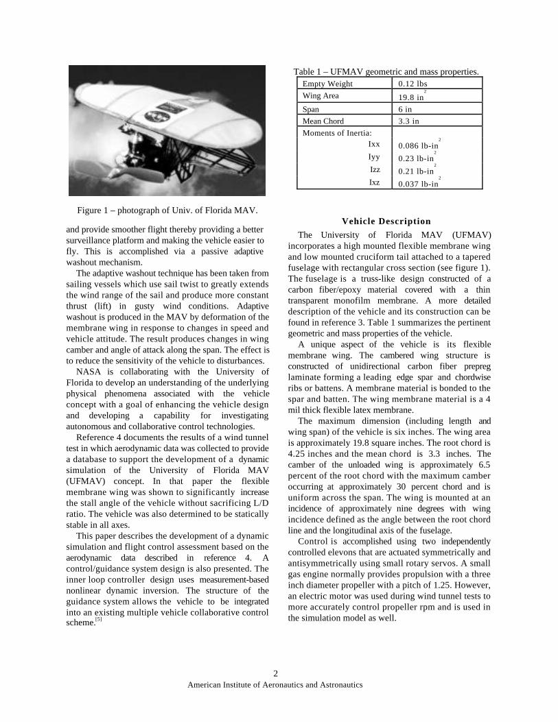
Table 1 – UFMAV geometric and mass properties.Empty Weight 0.12 lbs

Wing Area 19.8 in2

Span 6 in

Mean Chord 3.3 in

Moments of Inertia:Ixx 0.086 lb-in

2

Iyy 0.23 lb-in2

Izz 0.21 lb-in2

Ixz 0.037 lb-in2

Vehicle Description

The University of Florida MAV (UFMAV)incorporates a high mounted flexible membrane wingand low mounted cruciform tail attached to a taperedfuselage with rectangular cross section (see figure 1).The fuselage is a truss-like design constructed of acarbon fiber/epoxy material covered with a thintransparent monofilm membrane. A more detaileddescription of the vehicle and its construction can befound in reference 3. Table 1 summarizes the pertinentgeometric and mass properties of the vehicle.

A unique aspect of the vehicle is its flexiblemembrane wing. The cambered wing structure isconstructed of unidirectional carbon fiber prepreglaminate forming a leading edge spar and chordwiseribs or battens. A membrane material is bonded to thespar and batten. The wing membrane material is a 4mil thick flexible latex membrane.

The maximum dimension (including length andwing span) of the vehicle is six inches. The wing areais approximately 19.8 square inches. The root chord is4.25 inches and the mean chord is 3.3 inches. Thecamber of the unloaded wing is approximately 6.5percent of the root chord with the maximum camberoccurring at approximately 30 percent chord and isuniform across the span. The wing is mounted at anincidence of approximately nine degrees with wingincidence defined as the angle between the root chordline and the longitudinal axis of the fuselage.

Control is accomplished using two independentlycontrolled elevons that are actuated symmetrically andantisymmetrically using small rotary servos. A smallgas engine normally provides propulsion with a threeinch diameter propeller with a pitch of 1.25. However,an electric motor was used during wind tunnel tests tomore accurately control propeller rpm and is used inthe simulation model as well.


Simulation Model

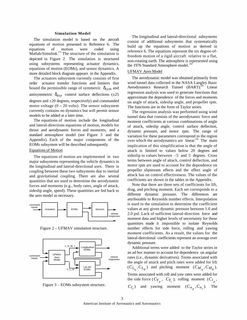
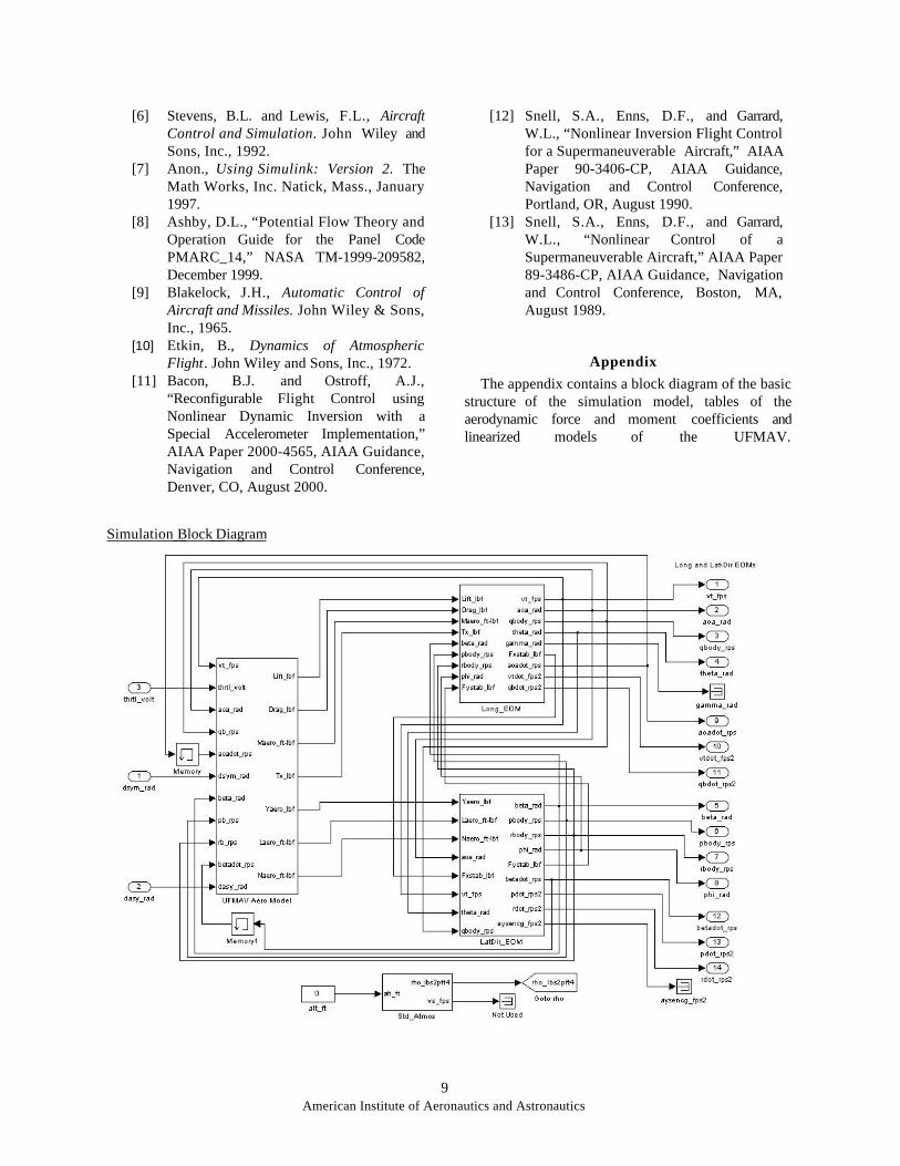
The simulation model is based on the aircraftequations of motion presented in Reference 6. Theequations of motion were coded usingMatlab/Simulink.[7] The structure of the simulation isdepicted in Figure 2. The simulation is structuredusing subsystems representing actuator dynamics,equations of motion (EOMs), and sensor dynamics. Amore detailed block diagram appears in the Appendix.

The actuators subsystem currently consists of firstorder actuator transfer functions and limiters thatbound the permissible range of symmetric δsym and

antisymmetric δasy control surface deflections (±25

degrees and ±20 degrees, respectively) and commandedmotor voltage (0 – 20 volts). The sensor subsystemcurrently contains no dynamics but will permit sensormodels to be added at a later time.

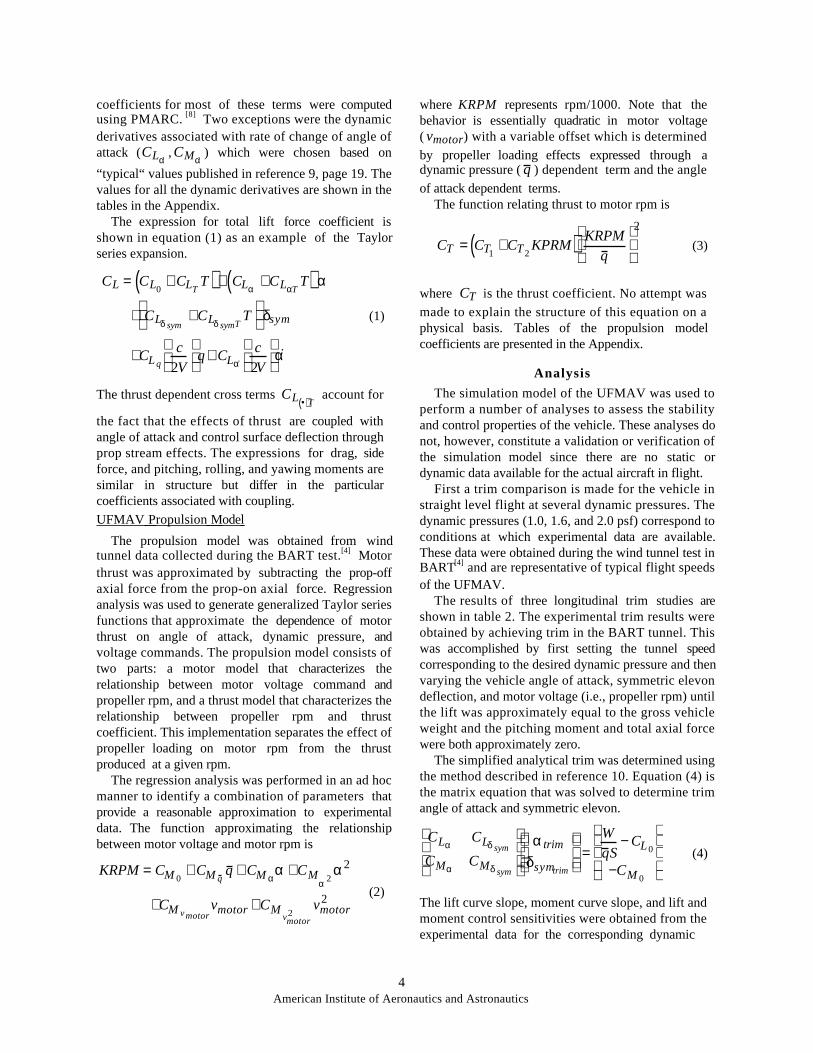
The equations of motion include the longitudinaland lateral-directions equations of motion, models forthrust and aerodynamic forces and moments, and astandard atmosphere model (see Figure 3 and theAppendix). Each of the major components of theEOMs subsystem will be described subsequently.

Equations of Motion

The equations of motion are implemented in twomajor subsystems representing the vehicle dynamics inthe longitudinal and lateral-directional axes. There iscoupling between these two subsystems due to inertialand gravitational coupling. There are also severalquantities that are used to determine the aerodynamicforces and moments (e.g., body rates, angle of attack,sideslip angle, speed). These quantities are fed back tothe aero model as necessary.

Actuators EOMs Sensors

commandinputs

vehicleresponses

Figure 2 – UFMAV simulation structure.

UFMAVAero

Model

LongitudinalEOMs

Lat–DirEOMs

commandinputs vehicle

responses

L, D, M, T

Y, L, N

Figure 3 – EOMs subsystem structure.

The longitudinal and lateral-directional subsystemsconsist of additional subsystems that systematicallybuild up the equations of motion as derived inreference 6. The equations represent the six degree-of-freedom motion of a rigid aircraft relative to a flat,non-rotating earth. The atmosphere is represented usingthe 1976 Standard Atmosphere model. [6]

UFMAV Aero Model

The aerodynamic model was obtained primarily fromwind tunnel data collected in the NASA Langley BasicAerodynamics Research Tunnel (BART).[4] Linearregression analysis was used to generate functions thatapproximate the dependence of the forces and momentson angle of attack, sideslip angle, and propeller rpm.The functions are in the form of Taylor series.

The regression analysis was performed using windtunnel data that consists of the aerodynamic force andmoment coefficients at various combinations of angleof attack, sideslip angle, control surface deflection,dynamic pressure, and motor rpm. The range ofvariation for these parameters correspond to the regionover which the aerodynamics are linear.[4] The mainimplication of this simplification is that the angle ofattack is limited to values below 20 degrees andsideslip to values between –5 and 5 degrees. Crossterms between angle of attack, control deflection, andmotor rpm are used to account for the dependence onpropeller slipstream effects and the effect angle ofattack has on control effectiveness. The values of thecoefficients are shown in the tables in the Appendix.

Note that there are three sets of coefficients for lift,drag, and pitching moment. Each set corresponds to adifferent dynamic pressure. The differences areattributable to Reynolds number effects. Interpolationis used in the simulation to determine the coefficientvalues at any given dynamic pressure between 1.0 and2.0 psf. Lack of sufficient lateral-direction force andmoment data and higher levels of uncertainty for thesequantities made it impossible to isolate Reynoldsnumber effects for side force, rolling and yawingmoment coefficients. As a result, the values for thelateral-directional coefficients represent an average overdynamic pressure.

Additional terms were added to the Taylor series inan ad hoc manner to account for dependence on angularrates (i.e., dynamic derivatives). Terms associated withthe angle of attack and pitch rates were added for lift(CLq

, CL ˙ α ) and pitching moment (CM q

, CM ˙ α ).

Terms associated with roll and yaw rates were added forthe side force (CYp

, CYr), rolling moment (Cl p

,

Clr) and yawing moment (Cn p

, Cnr). The


coefficients for most of these terms were computedusing PMARC. [8] Two exceptions were the dynamicderivatives associated with rate of change of angle ofattack (CL ˙ α

, CM ˙ α ) which were chosen based on

“typical“ values published in reference 9, page 19. Thevalues for all the dynamic derivatives are shown in thetables in the Appendix.

The expression for total lift force coefficient isshown in equation (1) as an example of the Taylorseries expansion.

CL = CL0+ CLT

T( )+ CLα+CLαT

T( ) α

+ CLδ sym+CLδ symT

T

δsym

+CLq

c2V

q + CL ˙ α

c2V

˙ α

(1)

The thrust dependent cross terms CL •( )T account for

the fact that the effects of thrust are coupled withangle of attack and control surface deflection throughprop stream effects. The expressions for drag, sideforce, and pitching, rolling, and yawing moments aresimilar in structure but differ in the particularcoefficients associated with coupling.

UFMAV Propulsion Model

The propulsion model was obtained from windtunnel data collected during the BART test.[4] Motorthrust was approximated by subtracting the prop-offaxial force from the prop-on axial force. Regressionanalysis was used to generate generalized Taylor seriesfunctions that approximate the dependence of motorthrust on angle of attack, dynamic pressure, andvoltage commands. The propulsion model consists oftwo parts: a motor model that characterizes therelationship between motor voltage command andpropeller rpm, and a thrust model that characterizes therelationship between propeller rpm and thrustcoefficient. This implementation separates the effect ofpropeller loading on motor rpm from the thrustproduced at a given rpm.

The regression analysis was performed in an ad hocmanner to identify a combination of parameters thatprovide a reasonable approximation to experimentaldata. The function approximating the relationshipbetween motor voltage and motor rpm is

KRPM = CM 0+ CM q

q + CM αα +CM

α 2α2

+CM v motorvmotor +CM

vmotor2

vmotor2 (2)

where KRPM represents rpm/1000. Note that thebehavior is essentially quadratic in motor voltage( vmotor) with a variable offset which is determined

by propeller loading effects expressed through adynamic pressure ( q ) dependent term and the angle

of attack dependent terms.The function relating thrust to motor rpm is

CT = CT1+CT2

KPRM( ) KRPMq

2

(3)

where CT is the thrust coefficient. No attempt was

made to explain the structure of this equation on aphysical basis. Tables of the propulsion modelcoefficients are presented in the Appendix.

Analysis

The simulation model of the UFMAV was used toperform a number of analyses to assess the stabilityand control properties of the vehicle. These analyses donot, however, constitute a validation or verification ofthe simulation model since there are no static ordynamic data available for the actual aircraft in flight.

First a trim comparison is made for the vehicle instraight level flight at several dynamic pressures. Thedynamic pressures (1.0, 1.6, and 2.0 psf) correspond toconditions at which experimental data are available.These data were obtained during the wind tunnel test inBART[4] and are representative of typical flight speedsof the UFMAV.

The results of three longitudinal trim studies areshown in table 2. The experimental trim results wereobtained by achieving trim in the BART tunnel. Thiswas accomplished by first setting the tunnel speedcorresponding to the desired dynamic pressure and thenvarying the vehicle angle of attack, symmetric elevondeflection, and motor voltage (i.e., propeller rpm) untilthe lift was approximately equal to the gross vehicleweight and the pitching moment and total axial forcewere both approximately zero.

The simplified analytical trim was determined usingthe method described in reference 10. Equation (4) isthe matrix equation that was solved to determine trimangle of attack and symmetric elevon.

CLαCLδ sym

CMαCMδ sym

α trim

δsymtrim

=

Wq S

− CL0

−CM 0

(4)

The lift curve slope, moment curve slope, and lift andmoment control sensitivities were obtained from theexperimental data for the corresponding dynamic


Table 2 – Experimental, analytical, and simulationbased longitudinal trim.

DynamicPressure

(psf)

PropellerRPM

Angle ofAttack(deg)

SymmetricElevon(deg)

Experimental Trim

1.0 18,900 10.4 -6.5

1.6 20,600 5.4 -3.5

2.0 21,900 4.0 -2.5

Analytical Trim (Simplified)

1.0 – 11.2 -5.6

1.6 – 5.4 -2.5

2.0 – 3.5 -1.9

Computed Trim (UFMAV)

1.0 19,600 11.1 -6.8

1.6 21,200 5.6 -4.7

2.0 22,000 3.5 -1.9

Table 3 – Computed lateral-directional trim.DynamicPressure

(psf)

SideslipAngle(deg)

BankAngle(deg)

AntisymmetricElevon(deg)

Computed Trim (UFMAV)

1.0 -0.051 -0.97 -0.59

1.6 0.028 -1.6 -0.54

2.0 0.070 -2.1 -0.51

pressure. [4] The data was assumed to correspond to apropeller rpm near trim.

The computed trim was obtained by using theUFMAV simulation model and a constraintedoptimization routine to achieve level trim at a specifieddynamic pressure. Comparison of the three trimanalyses shows very good agreement for angle ofattack, symmetric elevon deflection, and propeller rpm.This implies that the longitudinal aerodynamic forcesand moments are well approximated in the simulation.

A straight and level trim analysis using thesimulation model was also performed to determine thelateral-directional quantities: sideslip, bank, and yawangles. Table 3 shows the results of this analysis.Note that the UFMAV achieves lateral- directionalcontrol via antisymmetric elevon and dihedralcoupling. It does not have two independent lateral-directional controls (such as rudder and aileron) andcannot be trimmed at zero bank angle (or zero sideslipangle) as is typical. The results indicate that thoughthe vehicle does have significant asymmetries, all thetrim values are small and within the range of values atwhich the aerodynamic data was obtained and arequalitatively consistent with the vehicle in flight.

Table 4 – longitudinal modes.Short Period Mode Phugoid ModeDynamic

Pressure(psf)

dampingratio

freq.(rad/sec)

dampingratio

freq.(rad/sec)

1.0 0.13 23.3 0.44 0.85

1.6 0.12 30.2 0.35 0.65

2.0 0.12 32.6 -0.56 0.67

Table 5 – lateral-directional modes.SpiralMode

RollMode

Dutch Roll ModeDynamicPressure

(psf) eigenvalue eigenvalue dampingratio

freq.(rad/sec)

1.0 -1.04 -27.7 0.094 21.1

1.6 -1.04 -37.3 0.065 24.2

2.0 -1.02 -42.8 0.050 25.9

The simulation was also linearized about the abovetrim conditions to assess the dynamic stability of thevehicle. Table 4 summarizes the frequency anddamping of the linearized longitudinal modes. Notethat the short period mode is stable for all threedynamic pressures but lightly damped. Its frequencyincreases with increasing dynamic pressure but thedamping is essentially constant. The damping of thephugoid mode varies significantly and is unstable atthe higher dynamic pressure.

Table 5 summarizes the eigenvalues or frequencyand damping of the linearized lateral-directional modes.Note that all the modes are stable and that the dutchroll mode is lightly damped. This is qualitativelyconsistent with behavior of the vehicle in flight. Notethat the spiral mode is relatively unaffected by changesin dynamic pressure but that the magnitudes of boththe roll and dutch roll modes increase with increasingdynamic pressure.

Linearized models used to perform this analysis canbe found in the Appendix.

Control Design

A preliminary guidance/control system has beendeveloped to enable investigations of autonomous andcollaborative control issues. The controller iscomposed of two main parts: an inner-loopmeasurement-based nonlinear dynamic inversioncontroller for control of angular rates and an outer-loopnavigation command follower for control of wind-axisangles.[11,12] An overview of the control system isgiven in figure 4. The control system inputs arecommanded flight-path angle γ , wind-axis headingangle χ, and total speed V t. These inputs were chosento allow the vehicle to be readily integrated into anexisting multiple vehicle collaborative controlscheme.[5] Controller outputs are commanded symmetric


Figure 4 – structure of UFMAV control system.

and antisymmetric elevon deflection. A separateproportional-integral error loop is used to generatemotor voltage commands to control total velocity.For this preliminary study, the feedbackmeasurements are assumed to be known perfectly.The two main parts of the control system arediscussed in more detail in the following.

Measurement-based Nonli near Dynamic Inversion Given desired values of roll acceleration ˙ p , pitchacceleration ˙ q , and yaw acceleration ˙ r , the inner-

loop controller generates symmetric andantisymmetric elevon commands to achieve thedesired angular accelerations. The inner-loopcontroller is based on a modified nonlinear dynamicinversion approach developed in reference 11. Thisapproach does not require a model of the baselinevehicle (i.e. no stability derivatives), but does requirea model of the vehicle's control effector derivativesand feedback of body-axis angular accelerations andcontrol effector positions. Since this approach usesacceleration measurements in lieu of a complete on-board vehicle model, this approach is less sensitive tovehicle model errors and can adapt to vehicle failuresand/or damage. An overview of the approach fromreference 11 is given in the following.

Given the vehicle equations of motion

˙ x = F(x ,δ) = f (x) + g(x,δ)

y = p q r[ ]T = h(x)

where x is the vehicle state vector, δ is the vehiclecontrol vector, and y is the vector of controlvariables: roll rate p, pitch rate q, and yaw rate r. ATaylor series expansion of (5) yields the followingfirst-order approximation to F(x,δ) in theneighborhood of x0 ,δ0[ ]F(x,δ) = f (x0 )+ g(x0,δ0 )+

∂∂x

f (x) + g(x,δ)( )x=x 0,δ=δ0

(x − x0) −

∂∂δ

g(x ,δ)( )x=x 0 ,δ =δ0

(δ −δ0)

Letting x0 and δ0 denote a previous state and controlfrom the recent past and defining

A0 = ∂∂x

f (x)+ g(x,δ)( )x=x0 ,δ =δ 0

B0 = ∂∂δ

g(x,δ)( )x=x 0,δ=δ0

F(x,δ) can be written as

F(x,δ) = ˙ x ≅ ˙ x 0 + A0 (x − x0 )+ B0∆δ

in the neighborhood of x = x0 , δ =δ0 whereδ = δ0 + ∆δ .

At this point, this development differs fromreference 11 in that the number of controls is less thanthe number of controlled variables and so the desiredresponses cannot be completely achieved. A control lawis obtained by minimizing

J = ( ˙ y d − ˙ y )T Q( ˙ y d − ˙ y )

where

˙ y = ∂h(x )∂x

˙ x = hx ˙ x 0 + A0(x − x0) + B0∆δ( )and Q is a positive-definite diagonal weighting matrixused to emphasize desired system responses. Thisyields

∆δ = (hxB0 )T QhxB0[ ]−1(hxB0)T Q ⋅

˙ y d − hx ˙ x 0( )With a sufficiently fast update rate x tends to x0 andequation (11) becomes

∆δ = hxB0( )T QhxB0

−1

hxB0( )T Q ˙ y d − hx ˙ x 0( )

where δ = δ0 + ∆δ . The vehicle's control derivativesB0 are generated from the nonlinear aerodynamiccontrol coefficients using a central differenceapproximation.

Navigation Command Follower Given desired values of flight path angle γ , wind-axis heading χ, and total velocity V t the navigationcommand follower generates required roll rate, pitchrate, and yaw rate acceleration commands for theinner-loop controller.

The desired dynamics for the outer-loop were chosento be

(6)

(5)

(7)

(8)

(9)

(10)

(11)

(12)

CommandGenerator

NonlinearDynamicInversion

c

c

c

tV

γχ dy& cmdδ y


˙ γ d =ωγ (γc −γ)

˙ χ d = ωχ (χ c − χ)

where the subscript d denotes the desired value and thesubscript c denotes commanded input values. Thebandwidths ω χ and ω γ were chosen to beapproximately a decade below the bandwidths of thedesired inner-loop dynamics and therefore werechosen to be 2 rad/sec.

Using the wind-axis point mass equations of motionand assuming sideslip angle and sideforce are small andthat V t and cos(γ) are non-zero, commanded wind-axis bank angle µc can be determined as a function ofV t , ˙ γ

d and ˙ χ

d [13]

tanµc = Vt ˙ χ d cosγVt ˙ γ d + gcosγ

The desired dynamics for wind-axis bank angle waschosen to be

˙ µ d = ωµ (µc − µ )

where ω µ were chosen to be 4 rad/sec.The wind-axis angular rates ˙ µ , ˙ γ , and ˙ χ are

transformed to commanded body-axis rates (assumingsideslip angle is zero) using

pc

qc

rc

=cosα 0 −sinα

0 1 0

sinα 0 cosα

1 0 −sinγ0 cosµ sinµ cosγ0 −sinµ cosµ cosγ

˙ µ ˙ γ ˙ χ

where α is angle of attack. The desired closed-loopdynamics ˙ y

d for the inner-loop were chosen to be

˙ p d = ω p( pc − p )

˙ q d = ωq (qc − q )

˙ r d =ωr (rc −r)

where the subscript d denotes the desired value and thesubscript c denotes commanded values determined bythe outer-loop control law. The inner-loopbandwidths ω p, ω q, ω r were chosen to be 20, 15 and20 rad/sec, respectively, consistent with the open-loop bandwidth.

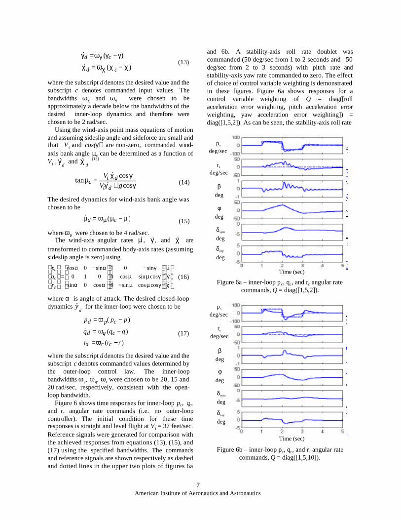
Figure 6 shows time responses for inner-loop pc, qc,and rc angular rate commands (i.e. no outer-loopcontroller). The initial condition for these timeresponses is straight and level flight at V t = 37 feet/sec.Reference signals were generated for comparison withthe achieved responses from equations (13), (15), and(17) using the specified bandwidths. The commandsand reference signals are shown respectively as dashedand dotted lines in the upper two plots of figures 6a

and 6b. A stability-axis roll rate doublet wascommanded (50 deg/sec from 1 to 2 seconds and –50deg/sec from 2 to 3 seconds) with pitch rate andstability-axis yaw rate commanded to zero. The effectof choice of control variable weighting is demonstratedin these figures. Figure 6a shows responses for acontrol variable weighting of Q = diag([rollacceleration error weighting, pitch acceleration errorweighting, yaw acceleration error weighting]) =diag([1,5,2]). As can be seen, the stability-axis roll rate

Figure 6a – inner-loop pc, qc, and rc angular ratecommands, Q = diag([1,5,2]).

Figure 6b – inner-loop pc, qc, and rc angular ratecommands, Q = diag([1,5,10]).

ps

deg/sec

rs

deg/sec

δsym

deg

δasy

deg

βdeg

φdeg

ps

deg/sec

rs

deg/sec

δsym

deg

δasy

deg

βdeg

φdeg

(13)

(14)

(15)

(16)

(17)

Time (sec)

Time (sec)


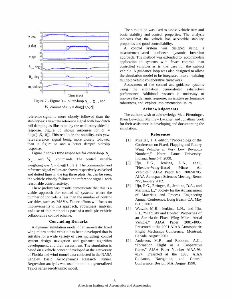
Figure 7 - Figure 3 – outer-loop γc

, χc

, and

Vtccommands, Q = diag([1,5,2]).

reference signal is more closely followed than thestability-axis yaw rate reference signal with low dutchroll damping as illustrated by the oscillatory sideslipresponse. Figure 6b shows responses for Q =diag([1,5,10]). This results in the stability-axis yawrate reference signal being more closely followedthan in figure 6a and a better damped sideslipresponse.

Figure 7 shows time responses for outer-loop γc

,

χc

, and Vtc commands. The control variable

weighting was Q = diag([1,5,2]). The commanded andreference signal values are shown respectively as dashedand dotted lines in the top three plots. As can be seen,the vehicle closely follows the reference signal withreasonable control activity.

These preliminary results demonstrate that this is aviable approach for control of systems where thenumber of controls is less than the number of controlvariables, such as, MAV's. Future efforts will focus onimprovements to this approach, robustness analysis,and use of this method as part of a multiple vehiclecollaborative control scheme.

Concluding Remarks

A dynamic simulation model of an aeroelastic fixedwing micro aerial vehicle has been developed that issuitable for a wide variety of uses including controlsystem design, navigation and guidance algorithmdevelopment, and their assessment. The simulation isbased on a vehicle concept developed at the Universityof Florida and wind-tunnel data collected in the NASALangley Basic Aerodynamics Research Tunnel.Regression analysis was used to obtain a generalizedTaylor series aerodynamic model.

The simulation was used to assess vehicle trim andbasic stability and control properties. The analysisindicates that the vehicle has acceptable stabilityproperties and good controllability.

A control system was designed using ameasurement-based nonlinear dynamic inversionapproach. The method was extended to accommodateapplication to systems with fewer controls thancontrolled variables as is the case for the subjectvehicle. A guidance loop was also designed to allowthe simulation model to be integrated into an existingmultiple vehicle collaborative framework.

Assessment of the control and guidance systemsusing the simulation demonstrated satisfactoryperformance. Additional research is underway toimprove the dynamic response, investigate performancerobustness, and explore implementation issues.

Acknowledgements

The authors wish to acknowledge Matt Pfenninger,Blain Levedahl, Matthew Lackner, and Jonathan Cookfor their assistance in developing and documenting thesimulation.

References

[1] Mueller, T. J. editor, “Proceedings of theConference on Fixed, Flapping and RotaryWing Vehicles at Very Low ReynoldsNumbers,” Notre Dame University,Indiana, June 5-7, 2000.

[2] Ifju, P.G., Jenkins, D.A., et.al.,“Flexible–Wing–Based Micro AirVehicles,” AIAA Paper No. 2002-0705.AIAA Aerospace Sciences Meeting, Reno,NV, January 2002.

[3] Ifju, P.G., Ettinger, S., Jenkins, D.A., andMartinez, L.,” Society for the Advancementof Materials and Process EngineeringAnnual Conference, Long Beach, CA, May6-10, 2001.

[4] Waszak, M.R., Jenkins, L.N., and Ifju,P.J., “Stability and Control Properties ofan Aeroelastic Fixed Wing Micro AerialVehicle.” AIAA Paper 2001-4005.Presented at the 2001 AIAA AtmosphericFlight Mechanics Conference. Montreal,Canada. August 2001.

[5] Anderson, M.R. and Robbins, A.C.,“Formation Flight as a CooperativeGame,” AIAA Paper Number AIAA-98-4124. Presented at the 1998 AIAAGuidance, Navigation, and ControlConference. Boston, MA. August 1998.

Time (sec)

γ deg

χ deg

Vt fps

δsym deg

δasy deg

mv volts


[6] Stevens, B.L. and Lewis, F.L., AircraftControl and Simulation. John Wiley andSons, Inc., 1992.

[7] Anon., Using Simulink: Version 2. TheMath Works, Inc. Natick, Mass., January1997.

[8] Ashby, D.L., “Potential Flow Theory andOperation Guide for the Panel CodePMARC_14,” NASA TM-1999-209582,December 1999.

[9] Blakelock, J.H., Automatic Control ofAircraft and Missiles. John Wiley & Sons,Inc., 1965.

[10] Etkin, B., Dynamics of AtmosphericFlight. John Wiley and Sons, Inc., 1972.

[11] Bacon, B.J. and Ostroff, A.J.,“Reconfigurable Flight Control usingNonlinear Dynamic Inversion with aSpecial Accelerometer Implementation,”AIAA Paper 2000-4565, AIAA Guidance,Navigation and Control Conference,Denver, CO, August 2000.

[12] Snell, S.A., Enns, D.F., and Garrard,W.L., “Nonlinear Inversion Flight Controlfor a Supermaneuverable Aircraft,” AIAAPaper 90-3406-CP, AIAA Guidance,Navigation and Control Conference,Portland, OR, August 1990.

[13] Snell, S.A., Enns, D.F., and Garrard,W.L., “Nonlinear Control of aSupermaneuverable Aircraft,” AIAA Paper89-3486-CP, AIAA Guidance, Navigationand Control Conference, Boston, MA,August 1989.

Appendix

The appendix contains a block diagram of the basicstructure of the simulation model, tables of theaerodynamic force and moment coefficients andlinearized models of the UFMAV.

Simulation Block Diagram


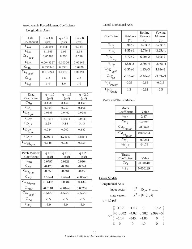
Aerodynamic Force/Moment Coefficients

Longitudinal Axes

LiftCoefficient

q = 1.0(psf)

q = 1.6(psf)

q = 2.0(psf)

CL 0 0.36094 0.341 0.344

CLα 3.1365 2.95 2.94

CLδ sym0.65369 0.590 0.590

CL T 0.0043367 0.00306 0.00169

CLαT 0.035346 0.0331 0.0228

CLδ symT 0.012241 0.00721 0.00394

CL q 4.0 4.0 4.0

CL ˙ α 1.0 1.0 1.0

DragCoefficient

q = 1.0(psf)

q = 1.6(psf)

q = 2.0(psf)

CD 0 0.150 0.162 0.157

CDα 0.304 0.257 0.166

CDδ sym0.0335 0.0462 0.0281

CD T -4.13e-3 -6.46e-4 0.0843

CDα 2 2.99 3.14 3.43

CDδ sym

2 0.224 0.202 0.182

CDT2 2.99e-4 8.24e-5 -3.83e-3

CDαδsym0.648 0.731 0.659

Pitch MomentCoefficient

q = 1.0(psf)

q = 1.6(psf)

q = 2.0(psf)

Cm 0 0.0797 0.0321 0.0304Cmα -0.470 -0.702 -0.741

Cmδ sym-0.350 -0.384 -0.355

Cm T 2.61e-4 1.26e-4 -4.86e-5Cmαδsym

0.14493 0.0884 0.136

CmαT -0.0118 -2.01e-3 0.00206Cmδ symT -5.51e-3 -4.52e-3 -2.52e-3

Cm q -0.5 -0.5 -0.5

Cm ˙ α -3.0 -3.0 -3.0

Lateral-Directional Axes

Coefficient Sideforce(Y)

RollingMoment

(l)

YawingMoment

(n)C •( )0 -1.91e-2 -4.72e-3 5.73e-3

C •( )β -8.55e-1 -2.74e-1 -3.25e-1

C •( )δ asy-5.72e-2 6.00e-2 3.00e-2

C •( )T 1.83e-3 2.70e-4 -2.46e-4

C •( )δ asyT-3.57e-3 1.25e-3 1.82e-3

C •( )βT-2.15e-2 -4.09e-3 -3.33e-3

C •( )pbody-0.35 -0.65 -0.015

C •( )rbody1.3 -0.32 -0.5

Motor and Thrust Models

MotorCoefficient Value

CM 0 2.17

CM q 0.0793

CM vmotor-0.0620

CMvmotor

2 0.000293

CM α -0.0264CM

α 2 -0.179

ThrustCoefficient Value

CT1 -0.00140

CT 2 0.000129

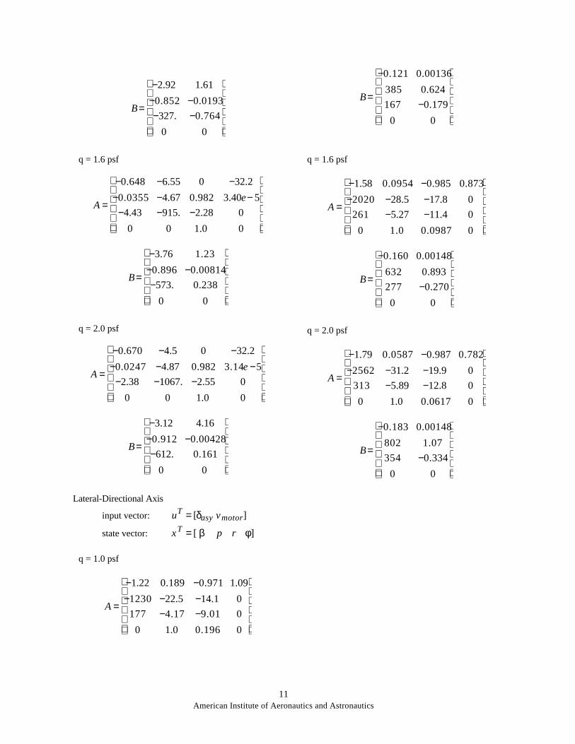
Linear Models

Longitudinal Axis

input vector: uT = [δsym vmotor]

state vector: xT = [Vt α q θ]

q = 1.0 psf

A =

−1.17 −11.3 0 −32.2

−0.0602 −4.02 0.982 2.99e −5

−5.14 −545. −1.80 0

0 0 1.0 0


B=

−2.92 1.61

−0.852 −0.0193

−327. −0.764

0 0

q = 1.6 psf

A =

−0.648 −6.55 0 −32.2

−0.0355 −4.67 0.982 3.40e− 5

−4.43 −915. −2.28 0

0 0 1.0 0

B=

−3.76 1.23

−0.896 −0.00814

−573. 0.238

0 0

q = 2.0 psf

A =

−0.670 −4.5 0 −32.2

−0.0247 −4.87 0.982 3.14e −5

−2.38 −1067. −2.55 0

0 0 1.0 0

B=

−3.12 4.16

−0.912 −0.00428

−612. 0.161

0 0

Lateral-Directional Axis

input vector: uT = [δasy vmotor]

state vector: xT = [ β p r φ]

q = 1.0 psf

A =

−1.22 0.189 −0.971 1.09

−1230 −22.5 −14.1 0

177 −4.17 −9.01 0

0 1.0 0.196 0

B=

−0.121 0.00136

385 0.624

167 −0.179

0 0

q = 1.6 psf

A =

−1.58 0.0954 −0.985 0.873

−2020 −28.5 −17.8 0

261 −5.27 −11.4 0

0 1.0 0.0987 0

B=

−0.160 0.00148

632 0.893

277 −0.270

0 0

q = 2.0 psf

A =

−1.79 0.0587 −0.987 0.782

−2562 −31.2 −19.9 0

313 −5.89 −12.8 0

0 1.0 0.0617 0

B=

−0.183 0.00148

802 1.07

354 −0.334

0 0

AIAA 2002-4875 Simulation and Flight Control of an Aeroelastic...

Documents

Transcript of AIAA 2002-4875 Simulation and Flight Control of an Aeroelastic...