AIAA-200_I-1236

ON THE ACCURACY OF PROBABILISTIC BUCKLING LOAD PREDICTIONS

Johann Arbocz*

Delft University of Technology, The Netherlandsand

James H. Starnes** and Michael P. Nemeth***

NASA Langley Research Center, Hampton, VA 23681-001

ABSTRACT

The buckling strength of thin-walled

stiffened or unstiffened, metallic or composite

shells is of major concern in aeronautical and

space applications. The difficulty to predict the

behavior of axially compressed thin-walled

cylindrical shells continues to worry design

engineers as we enter the third millennium.

Thanks to extensive research programs in the

late sixties and early seventies and the

contributions of many eminent scientists, it is

known that buckling strength calculations are

affected by the uncertainties in the definition of

the parameters of the problem such as

definition of loads, material properties,

geometric variables, edge support conditions

and the accuracy of the engineering models

and analysis tools used in the design phase.

The NASA design criteria monographs [1]

from the late sixties account for these design

uncertainties by the use of a lump sum safety

factor. This so-called "empirical knockdown

factor 7" usually results in overly conservative

design. Recently new reliability based

probabilistic design procedure for bucklingcritical imperfect shells have been proposed

[2,3]. It essentially consists of a stochastic

approach which introduces an improved"scientific knockdown factor Xa'', that is not as

conservative as the traditional empirical one.

In order to incorporate probabilistic

methods into a High Fidelity Analysis Approach

one must be able to assess the accuracy of the

various steps that must be executed to

Professor, Faculty of Aerospace

Engineering, Associate Fellow AIAA

Senior Engineer, Structures and Materials

Competency, Fellow AIAA

Senior Research Engineer, AssociateFellow AIAA

Copyright © 2001 by J. Arbocz, J.H.Starnes and M.P. Nemeth

Published by AIAA with permission

complete a reliability calculation. In the present

paper the effect of the size of the experimental

input sample on the predicted value of the

scientific knockdown factor Xa calculated by

the First-Order, Second-Moment Method is

investigated.

INTRODUCTION

Buckling strength of thin-walled stiffened

or unstiffened, metallic or composite shells is

of major concern in many aeronautical and

space applications. It is well known that the

critical buckling load is affected by theuncertainties in the definition of loads, material

properties, geometric variables, engineering

models and the accuracy of the analysis tools

used in the design phase. The NASA design

criteria from the late sixties account for these

design uncertainties by the use of a lump sum

safety factor, the so-called "knockdown" factor

¥[1], which usually results in an overly

conservative design.

Lately, probabilistic design procedures

have been proposed as a viable alternative

[2,3]. It is felt that quantifying and

understanding the "problem uncertainties" and

their influence on the design variables provides

an approach which will ultimately lead to a

better engineered, better designed and saferstructures.

However, the vast majority of practicing

engineers agree that true reliability must bedemonstrated and not just estimated from

analysis. It is the authors' opinion, that before

the engineering community will begin in large

numbers to accept the current generation of

probabilistic tools, two conditions must besatisfied. First, there must be test-constructed

data bases which can help in mapping the

input parameter uncertainties into probability

density functions. In addition, there must be

failure data bases, which can be used for test

verification of the probabilistic failure load

predictions.

1Ar_rir-on h'_efif,,f_ _f A_rr_no,,fir, c mnr'{ Ac:tr_n:mlltir'c_

https://ntrs.nasa.gov/search.jsp?R=20010071458 2018-05-13T07:02:19+00:00Z

It is generally agreed that, in order to make

the development of the Advanced Space

Transportation System a success and to

achieve the very ambitious performance goals

(like every generation of vehicles 10x safer and

10x cheaper than the previous one), one mustmake full and efficient use of the technical

expertise accumulated in the past 50 years or

so, and combine it with the tremendous

computational power now available. It is

obvious that with the strict weight constraints

used in space applications these performance

goals can only be achieved with an approach

often called "high fidelity analysis", where the

uncertainties involved in a design aresimulated by refined and accurate numerical

models. In the end the use of "high fidelity"numerical simulation will also lead to overall

cost reduction, since the analysis and design

phase will be completed faster and only the

reliability of the final configuration needs to be

verified by structural testing.

In order to incorporate probabilistic

methods into a High-Fidelity Analysis

Approach one must be able to assess the

accuracy of the various steps that must be

executed to complete a reliability calculation.

The central problem in the application of

stochastic processes is the estimation of the

various statistical parameters in terms of real

data. According to Papoulis [4], using

ensemble averaging to evaluate the lower

order statistical moments is appropriate if a

sufficiently large number of realizations of therandom vector X (m) are available.

This paper deals specifically with this

problem. To investigate the effect of the size of

the input sample on the predicted value of the

scientific knockdown factor Xa, the First-

Order, Second-Moment Method [3] is applied

successively to sample groups of differentsizes.

TEST PROGRAM

Using STONIVOKS [5], a special purpose

testing machine developed at the Structures

Laboratory of the Faculty of Aerospace

Engineering in Delft, a sample of 32 nominallyidentical seamless stainless steel "beer cans"

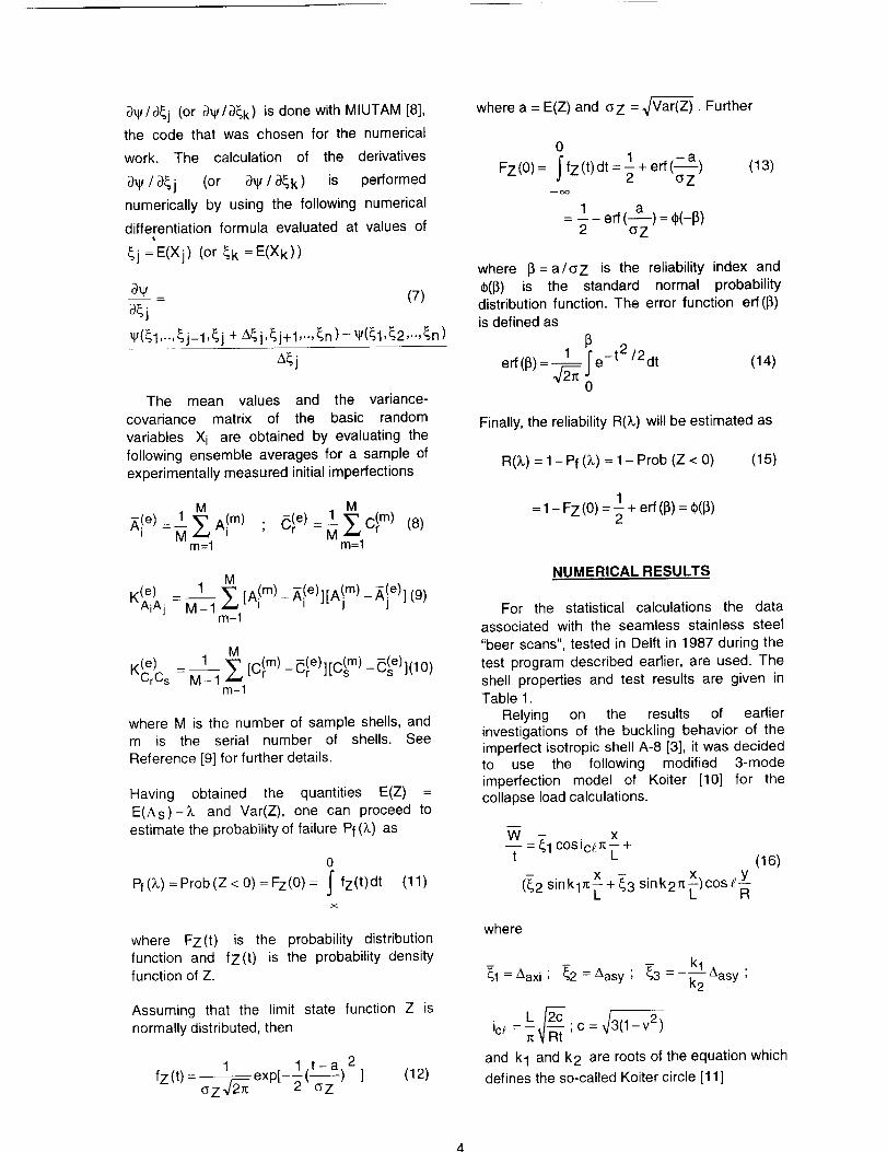
were tested. Figure 1 shows a typical test

specimen before top and bottom are cut off.

Figure 2 gives the general dimensions of a

typical specimen and shows the variation of

the wall thickness along 4 equally spaced

generators. Notice the increasing wall

thickness towards the open end of the can.

The imperfection surveys of the test-

specimen were carried out with the

STONIVOKS testing machine of the Delft

University of Technology (see Fig. 3). The

testing machine mainly consists of a rotating

platform on which the test specimen is placed,

and a vertical moving pick-up (LVDT

transducer). The shell is mounted between two

circular end discs. The top and bottom ends of

the can are cut off giving a cylinder of length100 mm. Next this specimen is placed betweenthe end disks in a circular channel which is

filled with molten "Cerrobend". When the

"Cerrobend" solidifies the edges of the cylinder

are fully clamped (Fig. 4). The rotary moment

of the platform and the vertical movement of

the pick-up are synchronized in such way that

one revolution of the specimen corresponds to

a vertical displacement of the pick-up by 1 mm.The number of measurements in the

circumferential direction is fixed at 100. Since

the usefull length of the cylinders is about 80

mm the number of measurements per test is

8000. As the rotary movement of the platform

(and subsequently the vertical movement of

the displacement pick-up) is continuous, the

measuring pattern is a helix over the outside

surface of the specimen. Figure 3 shows the

specimen installed in its testing position. For a

detailed discussion of this apparatus see Ref.

[5]. All buckling tests were preceded by a

complete imperfection survey controlled and

recorded by means of a Hewlett-Packard

HP9825S desktop calculator.

Data Reduction

The data reduction process involves 4

steps, namely: interpolation of the experiment-

al data, elimination of the rigid body motions, a

best fit correction, and finally a harmonic

analysis.

As stated before, the measuring pattern is a

helix over the outside surface of the test

specimen. In order to make the measurements

suitable for a harmonic analysis the imper-

fection data must be interpolated in axial

direction. Considering the error level present in

the measured data (due to the measuring

system) a linear interpolation is sufficient.

Although production and assembly of the

testing machine and the preparation of the test

specimen was very accurate, a certain amount

of rigid body motion of the test specimen was

unavoidable. This rigid body motion is mainlycaused by the fact that the center line of the

specimen never exactly coincides with the axis

of rotation of the platform.Becausetheabsolutevaluesof the imperfectionsaresmall,it is essential to correct the measuredimperfectionpattern for these rigid bodymotions.Tomeasurethisrigidbodymotion,apair of transducers (LVDT's) are used which

measure the displacements of the outer rim of

the two end disks. The outer rim of each disk is

considered to be concentric to a high degree.

An analysis of this rigid motion shows that the

displacements measured at the outer rim of the

end disks may be considered as to be

sinusoidal. After calculation of the average

displacements of each rim and subtracting this

value from the measured displacements on the

outer rim of the upper and lower ring a linear

interpolation of the measured imperfections inthe axial direction is carried out.

Before calculating the coefficients of the

double Fourier series representations of the

measured contours, it is necessary to

determine what is to be considered the perfect

shell. This is done by fitting a best-fit cytinder

(Fig. 5) to the measured data of the initial

imperfection scan. The method of least

squares is used to calculate the eccentricities

Xl, Y1, the rigid body rotations _1, £2 and the

mean radius R. Finally, the initial imperfections

are defined by recomputing the measured

distances with respect to the newly found

"perfect" cylinder. The recalculated radial initial

imperfections of the isotropic shell IWl-16 are

shown in Fig. 6. The coefficients of the

following double Fourier series, referenced to

the "best-fit cylinder"

_/(rn)(x, y) = tZ Alm) cos i_ L (1)i

+h__, Z sin k_X (C_r_) cos_ Y+D! m) sin,_ yL _. R _ R

k (/

are calculated numerically.

By assuming that the Fourier coefficients of

the initial imperfections are the basic random

variables Xi , we have a sample of 32 random

fields representing the 32 nominally identicalshells. For further details of the test-data the

interested reader should consult Ref. [6].

STOCHASTIC STABILITY ANALYSIS

The collapse problem of axially

compressed isotropic cylinders can best be

formulated in terms of a response (or limit

state) function

g(X) = As(X )- X (2)

where _=P/Pc is the suitabty normalized

load parameter, As is the random collapse

load of the shell, and the vector X represents

the Fourier coefficients of the initial

imperfections. Clearly the response function

g(X) = 0 separates the variable space into a

"safe region" where g(X)> 0, and a "failure

region" where g(X) < 0. The reliability R(X), or

the probability of failure Pf(;L) can then becalculated as

R(X) = 1 - Pf (,%) (3)

where

Pf (_,) = Prob {g(X) _<O} = f g(X.;_offX(X)dx (4)

The limit state function g(X), if so desired, can

be determined with great accuracy with

currently available nonlinear finite element

codes such as STAGS [7]. However, the

evaluation of the multi-dimensional probability

integral, where the domain of integration

depends on the shape of the response (or limit

state) function, is by no means trivial.

Using as an approximation the First-Order,Second-Moment Method to evaluate this

integral involves linearization of the response

function g(X)--> Z(X) at the mean point and

knowledge of the distribution of the randomvector X. To combine the use of numerical

codes with the mean value First-Order,

Second-Moment Method, one needs to know

the lower order probability characteristics of Z.

In the first approximation the mean value of Zis

E(Z) = E(As)- X= E[_U(Xl ..... Xn)]-;L (5)

_£LrE(X1) ..... E(X n )] - X

whereas the variance of Z is approximated by

var(Z) = (6)

n n _1/ cq_var(A s ) - _ _ (c-_-[-)(3--_-)cov( Xj, Xk )

j=l k=l r)_j _k

where cov(Xi,Xj) is the variance-covariance

matrix. The calculation of the value of

_[E(Xl) ..... E(Xn)], which is the deterministic

collapse load of the imperfect shell with mean

imperfection amplitudes, and of the derivatives

o-)_/o-)_j(or_lS_k ) isdonewithMIUTAM[8],the codethat waschosenfor the numericalwork. The calculationof the derivatives

o_ / (3_j (or 0_ / 0_k ) is performed

numerically by using the following numerical

differentiation formula evaluated at values of

_j =E(Xj) (or _k =E(Xk))

°qV- = (7)

• ({1 .... _j-I,_j+A{j,_j+I .... _n)-_(_1,_2 .... _n)

The mean values and the variance-

covariance matrix of the basic random

variables Xi are obtained by evaluating the

following ensemble averages for a sample of

experimentally measured initial imperfections

1 M M

AI e)--MEAl m) " _le) =ME1 c_m)m=l m=l

(8)

M1

K('_)j - M-1 E [Alm)- _'le)][Alm) - AI e)] (9)m-1

MK(e) 1

CrCs - M-1 E [c_m) -c(e)lrc(m)r,, s -C(se)](10)m-1

where M is the number of sample shells, andm is the serial number of shells. See

Reference [9] for further details.

Having obtained the quantities E(Z) =

E(As)-k and Var(Z), one can proceed to

estimate the probability of failure Pf (;k,) as

0

Pf (;L) = Prob(Z < 0) =Fz(0 ) = j' fz(t)dt (11)

where Fz(t) is the probability distribution

function and fz(t) is the probability densityfunction of Z.

Assuming that the limit state function Z is

normally distributed, then

1 lt-a 2

- exp[-_(-_Z) ] (12)fz(t) c_z 2.vf_

where a = E(Z) and (_Z = _. Further

0

FZ(0)= j'fz(t)dt=l+erf(-a) (13)2 (_Z

--o,o

_ 1 erf(a.._.a___.)=¢(_13)2 (_Z

where 13=a/(_Z is the reliability index and

¢(13) is the standard normal probability

distribution function. The error function err(13)is defined as

r)

erf(13)= 1 _e-t2/2dt (14)

0

Finally, the reliability R(X) will be estimated as

R(k) = 1-Pf (k) = 1- Prob (Z < 0) (15)

1= -- + erf (13)= ¢(13)1 - Fz (0) = 2

NUMERICAL RESULTS

For the statistical calculations the data

associated with the seamless stainless steel

"beer scans", tested in Delft in 1987 during the

test program described earlier, are used. The

shell properties and test results are given inTable 1.

Relying on the results of earlier

investigations of the buckling behavior of theimperfect isotropic shell A-8 [3], it was decidedto use the following modified 3-mode

imperfection model of Koiter [10] for thecollapse load calculations.

tW_= _lcosic_nL +

X

(_2 sinkln_ + _3 sink2n x) cOs_ yL

(16)

where

Iz.

_1 =Aaxi; _2 =Aasy ; _ =-_22Aasy ;

icf=L--n 2_t ;c=

and k 1 and k 2 are roots of the equation which

defines the so-called Koiter circle [11]

k2Rt(L)2 +f_2Rt 1R2 R_cc=2c 2c( ) -k ([)=0 (17)

The Koitercircleis the locusof a familyofmodesbelongingto the lowesteigenvalue;Lc =1.0,wherebydefinition

No Et2Xc - ;Nct =-- (18)

Nct cR

andNo istheappliedaxialcompressivestressresultant.Thecircumferentialwavenumber,_ischosensuchthat kI =1.ThisyieldsthefirstKoitertriad[8].Theratiosof theamplitudesofthe imperfectionsare chosensuch that thedirectionof the postbucklingpathcoincideswiththepathof steepestdescent,whichyieldsthemostadverseimperfectionshape[10].

If the measuredinitial imperfectionisrepresentedbythedoubleFourierseriesofEq(1) then its root-mean-squarevalue is bydefinition

2_R LA2ms...._ 1 _ 22_:RLJ" j'[W(x,y)] dxdy (19)

O O

t2 ^_-_ --2 nl n2

i=1 k=l, ¢=2

Thus

nl nl n2

Arms 2 = 1 A2 1

i=1 k=1,#=2

=A 2 . + A2asy (20)axl

Using the imperfection model of Eq. (16) the

corresponding equivalent imperfection

amplitudes are listed in Table 2.

In order to investigate the effect of the size

of the input sample on the predicted value of

the scientific knockdown factor Xa initially the

32 shells are divided in 8 groups of 4 shells

each. Next for every group a separate

reliability calculation is carried out using theFirst-Order, Second-Moment Method (FOSM).

When applying this method to the first group of4 shells each the mean buckling load has to be

calculated first. Using the imperfection model

of Eq. (16) with the mean values of the

corresponding equivalent imperfection

amplitudes listed in Table 3, the result of the

calculation is E(As) = 0.550629.

The derivatives _3_/_j are calculated as

follows. For the increment of the random

variable in Eq. (7), 1% of the original mean

value of the corresponding equivalent Fourier

coefficient is used, so that A_j = 0.01. E(Xj).

The calculated derivatives are listed in Table 4.

In this study the increments of the path

parameter are chosen in such a way that thelimit loads are found accurate to within 0.01%.

Next, using the sample variance-covariance

matrix displayed in Table 5, one can evaluate

the mathematical expectation and the varianceof Z. The results of these calculations are

E(Z) = 0.550629 - X and Var(Z) = 0.15108.10. -3 .

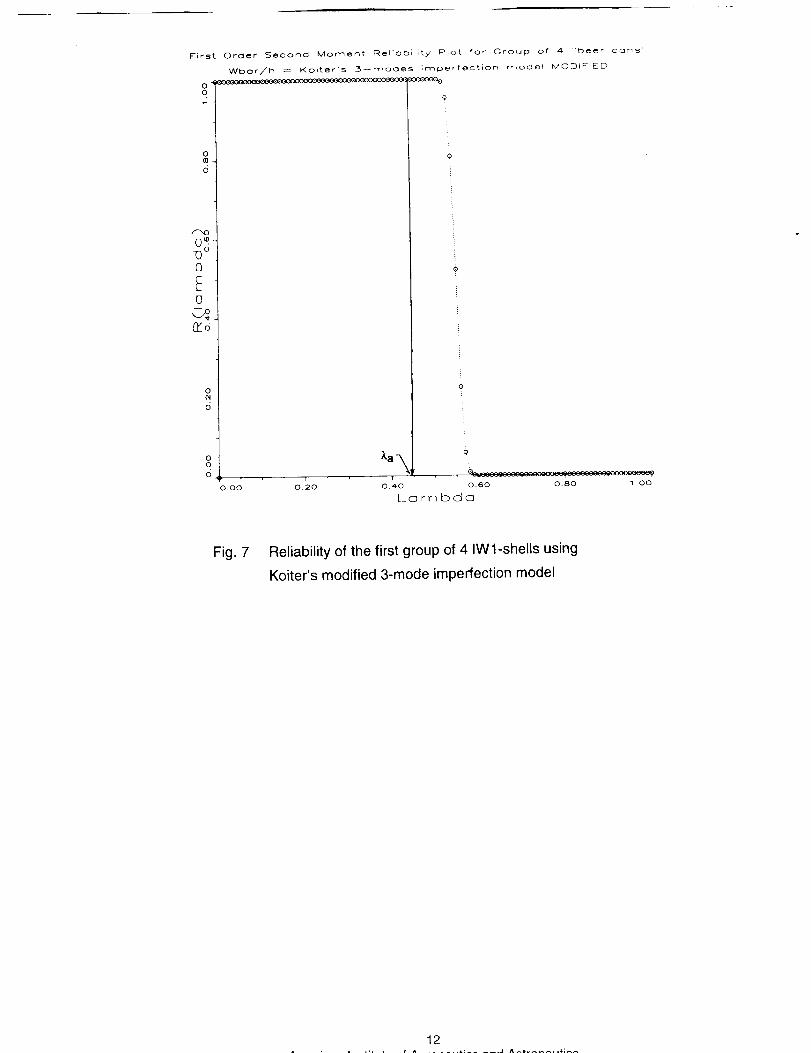
Finally, the reliability is calculated directly from

Eq. (15) and is plotted in Fig. 7. Notice that for

a reliability of 0.99999, one obtains a scientific

"knockdown" factor Xa = 0.49. Next the same

calculations must be repeated for the other

groups. The results of the calculations for the 8

groups of 4 shells each are summarized inTable 6. The results of similar calculations for 4

groups of 8 shells each and for 2 groups of 16shells each are shown in Tables 7 and 8

respectively. Using all 32 shells as one sample

group yields the following results:

E(Z)-0.552342-X ; o"z =0.0234049

and Xa =0.44 for a specified reliability of

R(X) = 0.99999.

CONCLUSIONS

A comparison of the "scientific knockdown

factors Xa" obtained with the different samplesizes listed in Table 8 indicates, that evaluating

the mean values and the variance-covariance

matrices via ensemble averaging of

experimental data yields accurate results if the

sample size is 16 or greater.

Comparing the probabilistic buckling load

Pa = XaPc_ = 0.44(-7909.734) = -3480.283 Ibs

which has a probability of failure of

Pf = 1-R(X) = 1-0.99999 = 0.1.10 -5

with the experimental buckling loads shown in

Table 1, it is seen that 3 of the test shellsbuckled below this value. Thus it is evident that

the simple initial imperfection model of Eq. (3)does not model the collapse behavior of the

shells tested accurately enough. In view of this

onemustconcludethatinorderto improvetheaccuracyof the probabilisticpredictionsto alevelrequiredbya "HighFidelityAnalysis",onemustinvestigatetheroleof usingmorerefinedmechanicalmodelsto calculatethe collapseloadsandemploymoreadvancemethodsforevaluatingthe multidimensionalprobabilityintegralof Eq.(4).

ACKNOWLEDGEMENT

The research reported in this paper was

supported in part by NASA Grant NAG 1-2129.

This aid is gratefully acknowledged.

REFERENCES

1. Anonymous, "Buckling of Thin-WalledCircular Cylinders", NASA SP-8007, 1968.

2. Ryan, R.S. and Townsend, J.S.,"Application of Probabilistic Analysis/

Design Method in Space Programs. TheApproaches, The Status and The Needs",

in: Proceedings 34th AIAA/ASME/ASCE/AHS/ASC Structures, Structural Dynamicsand Materials Conference, April 15-22,

1993, La Jolla, California, AIAA Paper No.93-1381.

3. Arbocz, J., Starnes, J.H. and Nemeth,

M.P., "Towards a Probabilistic Criterion

for Preliminary Shell Design", in:

Proceedings 39th AIAA/ASME/ASCE/AHS/ASC Structures, Structural Dynamics

and Materials Conference, April 20-23,1998, Long Beach, California, pp. 2941-2955.

4. Papoulis, A., "Probability, RandomVariables and Stochastic Processes",

Third Edition, McGraw-Hill InternationalEditions, Electrical & Electronic

Engineering Series, Singapore, 1991.5. Verduyn, W.D. and Elishakoff, I., "A

Testing Machine for Statistical Analysis ofSmall Imperfect Shells", Report LR-357,

Delft University of Technology, Faculty ofAerospace Engineering, September 1982.

6. Dancy, R. and Jacobs, D., "The InitialImperfection Data Bank at the Delft

University of Technology - Part I1", ReportLR-559, Delft University of Technology,

Faculty of Aerospace Engineering, June1988.

7. Brogan, F.A., Rankin, C.C. and Cabiness,H.D., "STAGS User Manual", Lockheed

Palo Alto Research Laboratory, ReportLMSC P032594, 1994.

8. Arbocz, J. and Babcock, C.D., Jr.,

"Prediction of Buckling Loads Based on

Experimentally Measured InitialImperfections", Proceedings IUTAM

Symposium "Buckling of Structures", B.Budiansky (Ed.), June 17-21, 1974,

Harvard University, Cambridge, MA,Springer Verlag, Berlin-Heidelberg-New

York, 1976, pp. 291-311.9. Elishakoff, I. and Arbocz, J., "Reliability of

Axially Compressed Cylindrical Shellswith General Nonsymmetric Imper-fections", Journal of Applied Mechanics,

Vol. 52, March 1985, pp. 122-128.10. Koiter, W.T., Personal Communication,

California Institute of Technology, April1974.

11. Koiter, W.T., "On the Stability of Elastic

Equilibrium", Ph.D. thesis (in Dutch), TH-Delft, The Netherlands. H.T. Paris,

Amsterdam, 1945. English translation

issued as NASA TT F-10, 1967, 833 p.

Table 1 Experimental buckling loads and geometric and material properties of the IWl-shells [6]

Pexp Pexp Pexp Pexp

IW1-16 3.05 IW1-24 4.27 IW1-33 4.03 IW1-42 3.82

-17 3.53 -26 3.99 -34 4.68 -43 3.83-18 4.50 -27 4.16 -36 4.43 -44 4.23-19 4.51 -28 4.24 -37 3.55 -45 3.99

-20 3.89 -29 4.49 -38 4.20 -46 3.35-21 4.01 -30 4.46 -39 4.00 -47 3.51-22 3.82 -31 4.47 -40 4.08 -48 3.43

-23 4.50 -32 4.01 -41 4.03 -49 3.48

For all shells: R=33.0mm ; t=0.1mm ; E=2.08.105N/mm 2 ; Pexp inkN

L = 100.0 mm v = 0.3

Table2 Equivalentimperfectionamplitudes

_/ _ cos32_L+_2sin_Xcos6Y+_.3sin31_Xcos6--y--_-= 1 L R L R

where_1= Aaxi; _2= Aasy; _3=-3.22581.10-2Aasy

Shell _1 _2 _ Shell _1 _2 _3

_W1-169.47549.10 -2 0.220433 -7.11075.10 -3 IW1-33 9.19913.10 -2 0.375521 -1.21136-10 -2

-17 9.56081-10 -2 0.263060 -8.48582.10 -3 -34 7.00014.10 -2 0.216141 -6.97230.10 -3

-18 8.48121.10 -2 0.206774 -6.67014.10 -3 -36 1.02874.10 -1 0.277256 -8.94375.10 -3

-19 8.36917.10 -2 0.229631 -7.40746.10 -3 -37 9.59792.10 -2 0.376076 -1.21315.10 -2

IWl-20 1.00125.10 -1 0.246147 -7.94023-10 -3 IWl-38 7.93719.10 -2 0.236075 -7.61533.10 -3

-21 8.48976.10 -2 0.217835 -7.02694.10 -3 -39 9.00877.10 -2 0.251087 -8.09959.10 -3

-22 9.29430.10 -2 0.376792 -1.21546.10 -2 -40 9.50537-10 -2 0.450460 -1.45310.10 -2

-23 8.53030.10 -2 0.259375 -8.36694.10 -3 -41 1.01069.10 -1 0.363866 -1.17376-10 -2

IWl-24 7.75164.10 -2 0.214565 -6.92146.10 -3 IWl-42 8.30259.10 -2 0.147869 -4.76997.10 -3

-26 9.81626.10 -2 0.260537 -8.40443.10 -3 -43 7.33546.10 -2 0.215469 -6.95062.10 -3

-27 9.92225.10 -2 0.306576 -9.88956-10 -3 -44 8.71149.10 -2 0.176853 -5.70494.10 -3

-28 7.57852-10 -2 0.148970 -4.80549.10 -3 -45 7.77785.10 -2 0.248184 -8.00594.10 -3

IW1-29 1.04704.10 -1 0.324469 -1.04668.10 -2 IWl-46 7.47830.10 -2 0.274016 -8.83924.10 -3

-30 6.66228.10 -2 0.250015 -8.06501-10 -3 -47 8.62856.10 -2 0.187197 -6.03862.10 -3

-31 7.04429.10 -2 0.166071 -5.3571310 -3 -48 7.67555-10 -2 0.187495 -6.04823.10 -3

-32 8.58714.10 -2 0.292634 -9.43982.10 -3 -49 8.66712-10 -2 0.245189 -7.90933.10 -3

Table 3 Values of random imperfections and

the sample mean vector

Table 4 Derivatives of

A s (X) = _[E(Xl) ..... E(X n)]

Xl(= _1) X2(= _2) X3(= _3-) Xj 8_/_Xj

IW 1-16 9.47549.10 -2 0.220433 -7.11075.10 _3 _1 = _/32.0 1 -1.6240-17 9.56081.10 -2 0.263060 -8.48582.10 -3

-18 8.48121.10 -2 0.206774 -6.67014.10 -3 _2 = _/1.6 2 -0.06349

-19 8.36917-10 -2 0.229631 -7.40746.10 -3: 3 1.9546

E( ) 8.97167.10 -2 0.229975 -7.41854-10 -3

Table 5 Sample variance-covariance matrix

1 2 3

1 0.40149.10 -4 Symmetric

2 0.87569.10 -4 0.57460.10 -3

3 -0.28248.10 -5 -0.18538.10 -4 0.59802-10 -6

Table 6 Reliability calculation for groups of 4 shells each

Group E(Z) o"z ;La

1 0.550629-X 0.0122915 0.49

2 0.543369-X 0.0156275 0.47

3 0.553647-X 0.0289698 0.42

4' 0.560122-X 0.0369662 0.39

5 0.540552-X 0.0282565 0.41

6 0.536736-X 0.0235181 0.43

7 0.571050-X 0.0080433 0.53

8 0.566009-X 0.0108056 0.51

Table 7 Reliability calculations for groups of 8 shells each

Group E(Z) o-z Xa

1 0.546944-X 0.0136657 0.48

2 0.556835-X 0.0307617 0.42

3 0.538439-X 0.0241657 0.43

4 0.568504-X 0.0092468 0.52

Table 8 Reliability calculations for groups of 16 shells each

Group E(Z) Gz Xa

1 0.551832-X 0.0232321 0.44

2 0.552866-X 0.0243072 0.44

Table 9 Influence of Sample Size on Reliability Predictions

Groups of 4 shells Groups of 8 shells Group of 16 shells Group of 32 shells

#1 Xa = 0.49

#2 Xa = 0.47 #1 _a = 0.48

#3 Xa = 0.42

#4 Xa = 0.39 #2 Xa = 0.42

#5 Xa =0.41

#6 Xa = 0.43 #3 Xa = 0.43

#7 Xa = 0.53

#8 ka = 0.51 #4 ka = 0.52

#1 Xa = 0.44

#2 Xa = 0.44 #1 Xa = 0.44

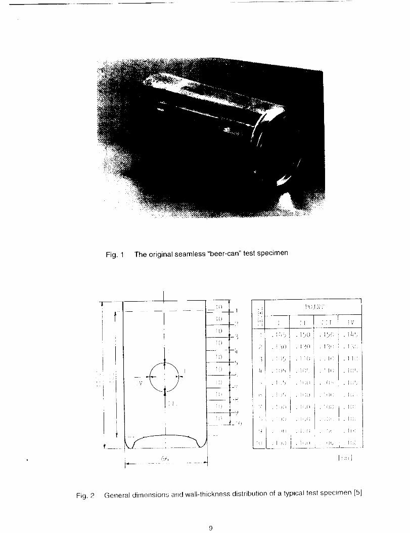
Fig. 1 The original seamless "beer-can" test specimen

-Pi,

ll i__ _i _

• ....J_ T,:̧)

, 1

L,

I

Ii{ :,

I [I_[1[ ]

Fig. 2 General dimensions and wall-thickness distribution of a typical test specimen [5]

Fig.3 Displacementpick-upsfor contourand rigidbodymotionmeasurements[5]

Fig.4 Test specimenwithenddisks

10

Z

i(x i.Y i ,z i)

._asuredpoint

X,Y,Z

XIY,'Z[

d i

Reference axis of

traversing pick-up

Ref.erence axis of

best fit cylinder

Normal distance

from measured point

to best fit cylinder

Fig. 5 Best-fit cylinder reference axes

L x

0.5L

0 _---_" 8=y/R

0 90 180 27'0 360

Fig. 6 Measured initial shape of the isotropic shell IW1-16 [6]

11

First Order Secomd Moment Rel_obillty Plot for Group of 4 "beer cans"

Wboc/h = KoiterIs 3--moctes imperfect}on nqodef MODIFVED

O 4 ...................... _oeeeee eo

00

0l

0,o0 0.20

0

0

E0

_d

0.40 0.60 0.80 1 O0

Lambda

Fig. 7 Reliability of the first group of 4 IWl-shells using

Koiter's modified 3-mode imperfection model

12