
AI .^fi3;. i^^a~iSM ;fi - Nuclear Regulatory Commission
173
cNWRAMO" O I AI ^ .^fi3;. i^^a~iSM ;fi _~ ~~~~~ 3 A A A Prepared for Nuclear Regulatory Commission Contract NRC-02-88-005 Prepared by Center for Nuclear Waste Regulatory Analyses San Antonlo, Texas August 1991 462.2 --- T 1 x9 1 0 - 1 6 CN 3 3ensit iivi t v a nd U ncret a-i n t v .5nalyses A-ppliei d to -- ye-D i mens i :iDra 1 TpendRck tP a L~ayer.e~d Fras turned Rr~rc .. a'r t
Transcript of AI .^fi3;. i^^a~iSM ;fi - Nuclear Regulatory Commission
cNWRAMO" O
I
AI ̂ .^fi3;. i^^a~iSM ;fi_~ ~~~~~ 3 A A A
Prepared for
Nuclear Regulatory CommissionContract NRC-02-88-005
Prepared by
Center for Nuclear Waste Regulatory AnalysesSan Antonlo, Texas
August 1991
462.2 --- T 1 x9 1 0 - 1 6 CN 33ensit iivi t v a nd U ncret a-i n t v.5nalyses A-ppliei d to-- ye-D i mens i :iDra 1 TpendRck tP
a L~ayer.e~d Fras turned Rr~rc .. a'r t
Property ofCNWRA Library CNVVRA 91-010
SENSITIVITY AND UNCERTAINTY ANALYSESAPPLIED TO ONE-DIMENSIONAL TRANSPORT IN A
LAYERED FRACTURED ROCK
PART 1: ANALYTIC SOLUTIONS AND LOCAL SENSHTIVITEES
Prepared for
Nuclear Regulatory CommissionContract NRC-02-88-005
Prepared by
A. B. GureghianY.-T. WuB. Sagar
Center for Nuclear Waste Regulatory AnalysesSan Antonio, Texas
and
R. B. Codell
Nuclear Regulatory CommissionOffice of Nuclear Materials Safety & Safeguards
August 1991

TABLE OF CONTENTS
Page
LIST OF FIGURES ..................... iiiLIST OF TABLES ..................... vACKNOWLEDGEMENTS ................... ixEXECUTIVE SUMMARY ..................... x
1. INTRODUCTION ................. 1-1
2. ANALYTICAL CONCENTRATIONS AND CUMULATIVE MASS 2-1
2.1. GOVERNING EQUATIONS .2-1
2.1.1. Initial and Boundary Conditions .2-22.1.2. Concentrations of the Source .2-32.1.3. Solution of Transport Equations for the Rock
Matrix and Fracture .2-4
2.1.3.1. Rock Matrix .2-42.1.3.2. Fracture .2-6
2.1.3.2.1. First Layer .2-72.1.3.2.2. Second Layer .2-92.1.3.2.3. Nth Layer .2-9
2.1.3.3. Rock Matrix .2-14
2.2.2.3.
CUMULATIVE MASS ......DISCUSSIONS OF RESULTS . .
2-162-22
2.3.1.2.3.2.
Case 1 Results .....Case 2 Results .....
....
... . .. 2-23
....
. .. .. . 2-55
3. ANALYTICALLY DERIVEDFRACTURE.
SENSITIVITIES IN THE. ..................... . 3-1
3.1 LOCAL SENSITVITIES.. . . . . . . . .3-1
i

TABLE OF CONTENTS (Continued)Page
3.2 ANALYTICAL SENSITIVITIES ........................ 3-1
3.2.1. Total Differentials .....................3.2.2. First Order Derivatives of the Concentrations ...3.2.3. First Order Derivatives of the Cumulative Mass
NUMNERICAL DERIVATIVES ...................VERIFICATION ............................
...
.... 3-1
..
. . ... 3-5
.
. .. 3-11
.
. .. 3-14
.
. .. 3-15
3.3.3.4.
4. CONCLUSIONS ......................................4-1
5. REFERENCES ....................................... 5-1
APPENDIX
A THEOREMS AND LAPLACE TRANSFORMS
B EVALUATION OF ERROR FUNCTION AND PRODUCT OFEXPONENTIAL AND COMPLEMENTARY ERROR FUNCTION TERMS
C SOME INTEGRALS INVOLVING THE ERROR FUNCTION AND OTHERFUNCTIONS
D FIRST ORDER DERIVATIVES OF THE COMPONENTS OF THECONCENTRATION SOLUTION IN THE FRACTURE LAYERS
E FIRST ORDER DERIVATIVES OF THE COMPONENTS OF THECUMULATIVE MASS SOLUTION IN THE FRACTURE LAYERS
F NOTATIONS
G MODEL PARAMETERS
ii

LIST OF FIGURES
Figure Title Page
1-1 Description of Migration Pathways in a System of Homogeneous Layers ofFractured Rock ......................................... 1-2
2-1 Source Models: (a) Exponentially Decaying, and (b) PeriodicallyFluctuating Decaying ..................................... 2-5
2-2(a) Relative Concentration of Np-237 vs. Distance in the Fracture at DifferentTimes T = 1,000, 5,000, and 50,000 years (ExponentiallyDecaying Source and Step and Band Release) ...................... 2-27
2-2(b) Relative Concentration of Np-237 in the Fracture vs. time at DifferentPositions x = 100 meters, 200 meters, and 500 meters (ExponentiallyDecaying Source) ....................................... 2-33
2-2(c) Cumulative Mass of Np-237 per Unit in the Fracture vs. Time at DifferentPositions x = 100, 200, and 500 meters (Exponentially Decaying Source andBand Release Mode) ..................................... 2-40
2-2(d) Relative Concentration of Np-237 in Rock-vs. Distance z at Time t = 5,000years and Distances from the Source x = 100, 200 and 500 meters(Exponentially Decaying Source and Step Release Mode) .............. 2-47
2-2(e) Relative Concentration of Np-237 in Rock vs. Distance at t = 50,000 years(Exponentially Decaying Source and Band Release Mode) .............. 2-51
2-3(a) Relative Concentration of Cm-245 vs. Distance in the Fracture at DifferentTimes t = 1,000, 5,000, and 50,000 years (PeriodicallyFluctuating Source with Exponential Decay) ...................... 2-59
2-3(b) Relative Concentration of Cm-245 in the Fracture vs. Time at DifferentPositions x = 100 meters, 200 meters, and 500 meters (PeriodicallyFluctuating Source with Exponential Decay) ...................... 2-65
2-3(c) Cumulative Mass of Cm-245 per Unit in the Fracture vs. Time at DifferentPositions x = 100, 200, and 500 meters (Periodically FluctuatingSource with Exponential Decay) ............................. 2-72
2-3(d) Relative Concentration of Cm-245 in Rock vs. Distance z at Time t = 5,000years and Distances from the Source x = 100, 200 and 500 meters(Periodically Fluctuating Source with Exponential Decay) .............. 2-79
iii

LIST OF FIGURES (Continued)
Figure Title Page
2-3(e) Relative Concentration of Cm-245 in Rock vs. Distance at t = 50,000years (Periodically Fluctuating Source with Exponential Decay) .... ...... 2-84
3-1(a) Sensitivity of Concentration to Half-thickness vs. Time for Np-237(Exponentially Decaying Source) ............................. 3-16
3-1(b) Sensitivity of Concentration to Pore Diffusivity vs. Time for Np-237(Exponentially Decaying Source) ............................. 3-16
3-1(c) Sensitivity of Concentration to Surface Distribution Coefficient inFracture vs. Time for Np-237 (Exponentially Decaying Source) .... ...... 3-17
3-1(d) Sensitivity of Concentration to Distribution Coefficient inRock vs. Time for Np-237 (Exponentially Decaying Source) .... ........ 3-17 i
3-2(a) Sensitivity of Cumulative Mass to Half-thickness vs. Time for Np-237(Exponentially Decaying Source) ............................. 3-18
3-2(b) Sensitivity of Cumulative Mass to Pore Diffusivity vs. Time for Np-237.(Exponentially Decaying Source) .............................. 3-18
3-2(c) Sensitivity of Cumulative Mass to Surface Distribution Coefficient inFracture vs. Time for Np-237 (Exponentially Decaying Source) .... ....... 3-19
3-2(d) Sensitivity of Cumulative Mass to Distribution Coefficient.in Rock vs.Time for Np-237 (Exponentially Decaying Source) .................. 3-19
iv
LIST OF TABLES
Table Title Page
2-1 Input Parameters for Case 1 Exponentially Decaying Source ..... . . . . . . 2-25
2-2(a) Case 1 Results: Concentration of Np-237 in the Fracture at Timet = 1,000 Years (Exponentially Decaying Source and Step Release Mode) .... 2-28
2-2(b) Case 1 Results: Concentration of Np-237 in the Fracture at Timet = 5,000 Years (Exponentially Decaying Source and Band Release Mode) ... 2-29
2-2(c) Case 1 Results: Concentration of Np-237 in the Fracture at Timet = 50,000 Years (Exponentially Decaying Source and Step Release Mode) . . . 2-30
2-3(a) Case 1 Results: Concentration of Np-237 in the Fracture Layer 2,at Distance x = 100 Meters (Exponentially Decaying Source andStep Release Mode) . 2-34
2-3(b) Case 1 Results: Concentration of Np-237 in the Fracture Layer 3,at Distance x = 200 Meters (Exponentially Decaying Sourceand Band Release Mode) ................. 2-36
2-3(c) Case 1 Results: Concentration of Np-237 in the Fracture Layer 5,at Distance x = 500 Meters (Exponentially Decaying Sourceand Band Release Mode) ..............................
2-4(a) Case 1 Results: Cumulative Mass of Np-237 in the Fracture at Distancex = 100 Meters (Exponentially Decaying Source and Band Release Mode)
2-4(b) Case 1 Results: Cumulative Mass of Np-237 in the Fracture at Distancex = 200 Meters (Exponentially Decaying Source and Band Release Mode)
2-4(c) Case 1 Results: Cumulative Mass of Np-237 in the Fracture at Distancex = 500 Meters (Exponentially Decaying Source and Band Release Mode)
2-5(a) Case 1 Results: Concentration of Np-237 in the Rock Matrix Layer 2,at Distance x = 100 Meters and Time t = 5,000 years (ExponentiallyDecaying Source and Step Release Mode) ....................
* . . . 2-38
. .. 2-41
. . . 2-43
. . . 2-45
.... 2-48
2-5(b) Case 1 Results: Concentration of Np-237 in the Rock Matrix Layer 3,at Distance x = 200 Meters and Time t = 5,000 years (ExponentiallyDecaying Source and Step Release Mode) .................... .... 2-49
v
LIST OF TABLES (Continued)
Table Title Page
2-5(c) Case 1 Results: Concentration of Np-237 in the Rock Matrix Layer 5,at Distance x = 500 Meters and Time t = 5,000 years (ExponentiallyDecaying Source and Step Release Mode) ........................ 2-50
2-6(a) Case 1 Results: Concentration of Np-237 in the Rock Matrix Layer 2,at Distance x = 100 Meters and Time t = 50,000 years (ExponentiallyDecaying Source and Band Release Mode) .................
2-6(b) Case 1 Results: Concentration of Np-237 in the Rock Matrix Layer 3,at Distance x = 200 Meters and Time t = 50,000 years (ExponentiallyDecaying Source and Band Release Mode) .................
. . . 2-52
. . . 2-53
2-6(c) Case 1 Results: Concentration of Np-237 in the Rock Matrix Layer 3,at Distance x = 500 Meters and Time t = 50,000 years (ExponentiallyDecaying Source and Band Release Mode) ....................... 2-54
2-7 Input Parameters for Case 2 Periodically Fluctuating Source withExponential Decay ..................................... 2-57
2-8(a) Case 2 Results: Concentration of Cm-245 in the Fracture at Timet = 1,000 Years (Periodically Fluctuating Source with ExponentialDecay and Step Release Mode) .............................. 2-60
2-8(b) Case 2 Results: Concentration of Cm-245 in the Fracture at Timet = 5,000 Years (Periodically Fluctuating Source with ExponentialDecay and Band Release Mode) .......................
2-8(c) Case 2 Results: Concentration of Cm-245 in the Fracture at Timet = 50,000 Years (Periodically Fluctuating Source with ExponentialDecay and Band Release Mode) .......................
2-9(a) Case 2 Results: Concentration of Cm-245 in the Fracture in Layer 2,at Distance x = 100 meters (Periodically Fluctuating Source withExponential Decay and Step Release Mode) ................
2-9(b) Case 2 Results: Concentration of Cm-245 in the Fracture in Layer 3,at Distance x = 200 meters (Periodically Fluctuating Source withExponential Decay and Band Release Mode) ...............
. ... .. . .2-61
. .. . .. . .2-62
....... . .2-66
....... . .2-68
vi

LIST OF TABLES (Continued)
Table Title Page
2-9(c) Case 2 Results: Concentration of Cm-245 in the Fracture in Layer 5,at Distance x = 500 meters (Periodically Fluctuating Source withExponential Decay and Band Release Mode) ...............
2-10(a) Case 2 Results: Cumulative Mass of Cm-245 in the Fracture atDistance x = 100 Meters (Periodically Fluctuating Source withExponential Decay and Band Release Mode) ...............
2-10(b) Case 2 Results: Cumulative Mass of Cm-245 in the Fracture atDistance x - 200 Meters (Periodically Fluctuating Source withExponential Decay and Band Release Mode) ...............
2-10(c) Case 2 Results: Cumulative Mass of Cm-245 in the Fracture atDistance x - 500 Meters (Periodically Fluctuating Source withExponential Decay and Band Release Mode) ...............
I. .. . ... 2-70
2-73
2-75
2-77
2-11(a) Case 2 Results: Concentration of Cm-245 in the Rock Matrix Layer 2,at Distance x = 100 Meters and Time t = 5,000 years (PeriodicallyFluctuating Source with Exponential Decay and Step Release Mode) . . ..
. . .. . 2-80
2-11(b) Case 2 Results: Concentration of Cm-245 in the Rock Matrix Layer 3,at Distance x = 200 Meters and Time t = 5,000 years (PeriodicallyFluctuating Source with Exponential Decay and Step Release Mode) ........ 2-81
2-11(c) Case 2 Results: Concentration of Cm-245 in the Rock Matrix Layer 5,at Distance x = 500 Meters and Time t = 5,000 years (PeriodicallyFluctuating Source with Exponential Decay and Step Release Mode)..
2-12(a) Case 2 Results: Concentration of Cm-245 in the Rock Matrix Layer 2,at Distance x = 100 Meters and Time t = 50,000 years (PeriodicallyFluctuating Source with Exponential Decay and Band Release Mode)
2-12(b) Case 2 Results: Concentration of Cm-245 in the Rock Matrix Layer 3,at Distance x = 200 Meters and Time t = 50,000 years (PeriodicallyFluctuating Source with Exponential Decay and Band Release Mode)
2-12(c) Case 2 Results: Concentration of Cm-245 in the Rock Matrix Layer 5,at Distance x = 500 Meters and Time t = 50,000 years (PeriodicallyFluctuating Source with Exponential Decay and Band Release Mode)
...
.. .. 2-82
...
.. .. 2-85
... . .. . 2-86
... .. .. 2-87
vii
LIST OF TABLES (Continued)
Table Title Page
3-1 First Order Partial Derivatives of 0,. with Respect to Input Parameters a; ..... 3-6
3-2 First Order Partial Derivatives of y., with Respect to Input Parameters ai ..... 3-7
3-3 First Order Partial Derivatives of cfi with Respect to Input Parameters a; ..... . 3-8
3-4 First Order Partial Derivatives of R, with Respect to Input Parameters a; ..... . 3-9
3-5 First Order Partial Derivatives of F'x with Respect to Input Parameters a; ..... . 3-9
A.1. Laplace Transforms .. A-2
viii

ACKNOWLEDIGMENTS
Several people assisted in the preparation of this report. The authors would like to express theirappreciation for their efforts which greatly helped the document to reach its final form.
In particular, we would like to thank Drs. W. C. Patrick and R. Ababou for their reviews,Mr. A. Johnson and Ms. L. Tweedy for their graphical contributions, Messrs. E. Perez and D.Saathoff, of the Computer and Telecommunication Center, and Mrs. M. A. Gruhlke, whoassisted in the coordination and production of this document.
ix

EXECUTIVE SIMLARY
Mathematical models have become essential tools in performance assessment investigations, forestimating the potential impact of radionuclide migration out of a HLW geologic repository tothe biosphere. These models involve a mathematical description of hydro-geochemical and -geo-physical processes, and their predictive capabilities are usually commensurate with ourunderstanding of the various classes of geologic media: porous and fractured rock. Currently,the candidate HLW disposal site is one which is located in fractured tuff. Since this geologicalmedium is poorly understood because of its inherent structural uncertainties and currently thereis a limited ability to quantitatively describe geological processes in that medium, the use ofsimplified mathematical models for a conservative probabilistic assessment of performance isappropriate. Moreover, in spite of their limitations the high degree of precision of analyticalmodels coupled with their computational efficiency have induced many investigators worldwide(Rosinger and Tremaine (1978), Hodgkinson and Maul (1985), Rasmuson and Neretnieks (1986),and Burkholder et al., (1976)) to adopt these for addressing some of the critical issues inherentto the containment characteristics of potential radioactive waste disposal sites.
This report is presented in two parts.
Part 1 reports the derivation and verification of the closed form analytical solutions of the one-dimensional non-dispersive and isothermal transport of a radionuclide in a layered system ofsaturated planar fractures coupled with diffusion into the adjacent saturated rock matrix. Inaddition to matrix diffusion effects as reported by Grisak et al., (1981, 1980) and Neretnieks(1980) (see also Gureghian (1990a) for a comprehensive list of references) on the one hand, andnon-zero initial conditions in both fracture and rock as illustrated by Gureghian (1990b) on theother, three new features associated with 1) the layered nature of the rock matrix, 2) the lengthdependency of fracture aperture, and 3) periodicity aspect of radionuclides released from thesource have been implemented in these new solutions.
Part 2 evaluates and demonstrates the use of several sensitivity and uncertainty analysis methodsusing the analytical model developed in Part 1.
The mathematical model "MULTFRAC" associated with Part 1 of this report includes twomodules. The first module predicts the space-time dependent concentration of a decaying speciesmigrating within the fracture network and the surrounding rock matrix layers, including thecumulative mass at an arbitrary observation point within the fracture. Note that the steadyunidirectional flow of water through the fracture is normal to the rock matrix layers. Moreover,the material properties of individual fracture and rock matrix layers assumed to be fullysaturated, are homogeneous and isotropic. The second module predicts the analytical andnumerical local sensitivities i.e., the first order derivatives of the concentration and cumulativemass with respect to the dependent variables. These are basic requirements for parameterestimation or sampling design in the case of the concentration, and for uncertainty analysis ofcumulative releases of a typical species from the repository at a typical point in time along thefracture as illustrated in Part 2 of this report.
x

The analytical solutions are based on the Laplace transform method where the domains ofradionuclide migration in both fractures and rock layers are one-dimensional and of the semi-infinite type, implying in this instance that radionuclide diffusion from the fractures wall to therock matrix may extend to infinity. The sorption phenomena in both fracture and rock matrixlayers are described by a linear equilibrium sorption isotherm. Two types of radionucliderelease modes are considered: the continuously decaying and the periodically fluctuatingdecaying source, which may in turn be subject to step and band release modes. The initialconcentrations in the fracture and rock matrix layers may be assigned spatially varying valuesin the case of the first whereas uniform ones may be implemented in both cases.
The verification of the new analytical solutions pertaining to solute transport in fracture and rockmatrix was performed by means of several well established numerical evaluation methods ofLaplace inversion integral proposed by Talbot (1979), Durbin (1974), and Stefhest (1970). Twotest cases involving the migration of Np-237 and Cm-245, in a five-layered fractured rocksystem were investigated. An evaluation of some of these inversion methods over the range ofinvestigated parameters have also been reported. On the other hand, the verification of theanalytical solutions for the local sensitivities of the concentration and cumulative mass in thefracture with respect to the parameters of the system was performed by means of numericaldifferentiation techniques based on the finite-difference method of approximation.
APPLICATIONS
The deterministic solutions presented in Part 1 of this report are primarily related to performanceassessment investigations of potential nuclear waste repository sites restricted to typical scenarioanalyses associated with long term migration of radionuclides in an idealized fractured rocksystem. The new predictive capabilities imbedded in the derived solutions are expected toimprove the confidence of the investigator performing sensitivity and uncertainty analyses basedon this model.
The model MULTFRAC was written in VAX FORTRAN Version 4.8 using the G floating pointoption (REAL*16). The computation was executed on a VAX 8700 under VMS Version 4.7.
xi
U
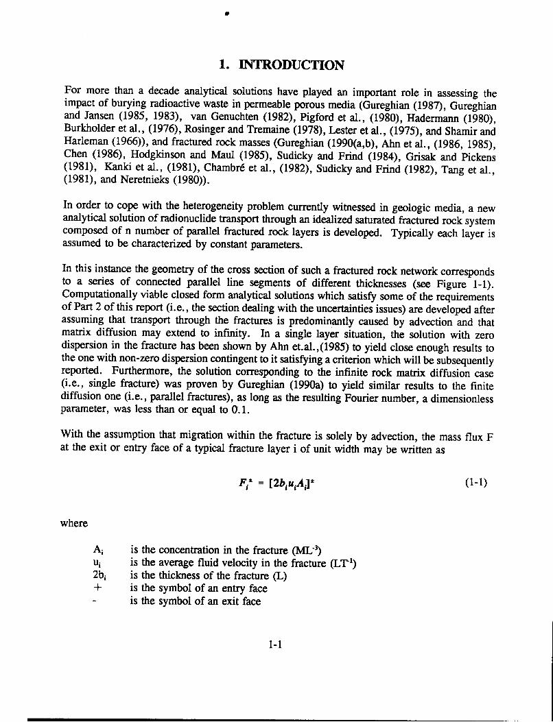
1. INTRODUCTION
For more than a decade analytical solutions have played an important role in assessing theimpact of burying radioactive waste in permeable porous media (Gureghian (1987), Gureghianand Jansen (1985, 1983), van Genuchten (1982), Pigford et al., (1980), Hadermann (1980),Burkholder et al., (1976), Rosinger and Tremaine (1978), Lester et al., (1975), and Shamir andHarleman (1966)), and fractured rock masses (Gureghian (1990(a,b), Ahn et al., (1986, 1985),Chen (1986), Hodgkinson and Maul (1985), Sudicky and Frind (1984), Grisak and Pickens(1981), Kanki et al., (1981), Chambrd et al., (1982), Sudicky and Frind (1982), Tang et al.,(1981), and Neretnieks (1980)).
In order to cope with the heterogeneity problem currently witnessed in geologic media, a newanalytical solution of radionuclide transport through an idealized saturated fractured rock systemcomposed of n number of parallel fractured rock layers is developed. Typically each layer isassumed to be characterized by constant parameters.
In this instance the geometry of the cross section of such a fractured rock network correspondsto a series of connected parallel line segments of different thicknesses (see Figure 1-1).Computationally viable closed form analytical solutions which satisfy some of the requirementsof Part 2 of this report (i.e., the section dealing with the uncertainties issues) are developed afterassuming that transport through the fractures is predominantly caused by advection and thatmatrix diffusion may extend to infinity. In a single layer situation, the solution with zerodispersion in the fracture has been shown by Ahn et.al.,(1985) to yield close enough results tothe one with non-zero dispersion contingent to it satisfying a criterion which will be subsequentlyreported. Furthermore, the solution corresponding to the infinite rock matrix diffusion case(i.e., single fracture) was proven by Gureghian (1990a) to yield similar results to the finitediffusion one (i.e., parallel fractures), as long as the resulting Fourier number, a dimensionlessparameter, was less than or equal to 0.1.
With the assumption that migration within the fracture is solely by advection, the mass flux Fat the exit or entry face of a typical fracture layer i of unit width may be written as
Fit = [2bjujAiJ. (1-)
where
Ai is the concentration in the fracture (ML;')ui is the average fluid velocity in the fracture (LT")2bi is the thickness of the fracture (L)+ is the symbol of an entry face- is the symbol of an exit face
1-1

z10-
I~~~zHLW Source X
Li U1 Kf i2b 1 O, Dp1 P1 Kr1 Layer 1
L 2 U2Kf2 2b2 (2 DpP2 K Layer 2
L3 Fracture Layer 3
-un Kfn Layer------
L un Kfn _ . 2bn On DPn Pn Krn Layer n
Figure 1-1. Description of Migration Pathways in a System of Homogeneous Layers ofFractured Rock. (See Appendix F for definition of symbols.)
1-2
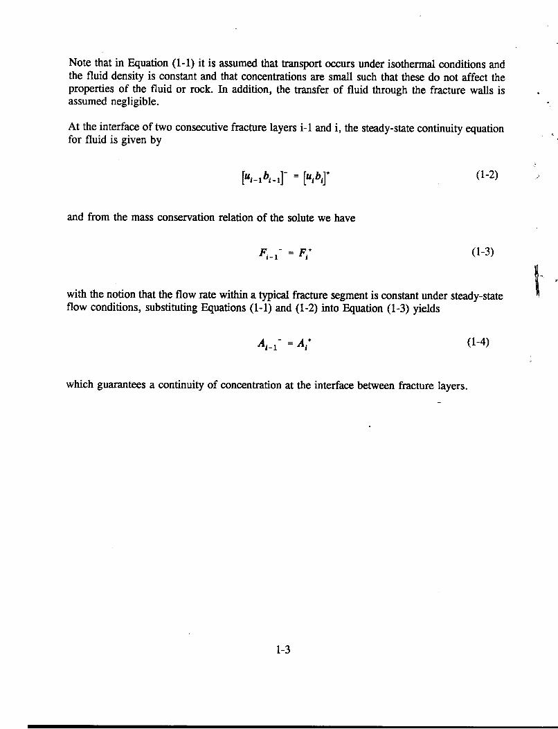
Note that in Equation (1-1) it is assumed that transport occurs under isothermal conditions andthe fluid density is constant and that concentrations are small such that these do not affect theproperties of the fluid or rock. In addition, the transfer of fluid through the fracture walls isassumed negligible.
At the interface of two consecutive fracture layers i-l and i, the steady-state continuity equationfor fluid is given by
[lub 1 1p = [uibi] (1-2)
and from the mass conservation relation of the solute we have
F-jl- = Fj+ (1-3)
with the notion that the flow rate within a typical fracture segment is constant under steady-stateflow conditions, substituting Equations (1-1) and (1-2) into Equation (1-3) yields
Ai-1- = Ai+ (1-4)
which guarantees a continuity of concentration at the interface between fracture layers.
1-3

2. ANALYTICAL CONCENTRATIONS AND CUMULATIVE MASS
2.1. GOVERNING EQUATIONS
The governing one-dimensional equation describing the non-dispersive movement of atypical nuclide in the ith layer of the fracture and rock matrix respectively (Neretnieks, 1980)is given by
(a) Fracture
Ri + ui i + URAi +- = 0, xi ,<x•X, (2-1)ax bi
(b) Rock Matrix
Mi d1B, ~~~~~~~~~~~(-2)A!- - Dpi + A R!B, = ° (2-2
at~a
too , x >0, z 2tbi i = 1,,3,...,n
whereR, is the retardation in the fractureX is the first-order rate constant for decay (T 1)Hi is the diffusive rate of radionuclide at surface of fracture per unit area of fracture
surface (MI2TI')
R! is the retardation factor in the rock matrixB.; is the concentration in the rock matrix (MU3)Dp; is the pore diffusivity (1;2T')x is the spatial coordinate in the fracture (L)z is the spatial coordinate in the rock matrix (L)t is the time ()i is the index related to the particular layer of fracture and surrounding rock
matrixn is the total number of fractured rock layers
A complete list of symbols and their meanings is given in Appendix F.
2-1

The diffusive rate of a nuclide into the ith layer of the rock matrix is assumed to obeyFick's law of diffusion written as
azJ D ABI (2-3)
where D,. is the effective diffusivity in the typical section of the rock matrix (see Neretnieks,1980) defined as
DeL = 0 P (2-4)
where,t; is the rock porosityDO is the pore diffusivity (i.e., Dpi= Ddg,) (L9 T1')Dd is the molecular diffusion of nuclide in water (L 2T-1)gfi is. the geometric factor (6di /hr2) whereadi is constrictivity for diffusion (LI)Ti is tortuosity of rock matrix (LU)
The retardation factor in the ith layer of the fracture (R;) and the rock matrix (R.), respectively(see Neretnieks et al., 1982), are given by:
Ri = 1 + bft (2-5)
= 1 + [(l-@g)I0 1 ]PnKn (2-6)
whereP i is the bulk rock density (ML)Kfi is the surface distribution coefficient in the fracture (L)Ki is the distribution coefficient in the rock matrix (L 3M')
2.1.1. Initial and Boundary Conditions
The set of differential equations, Equations (2-1) and (2-2), are subject to theinitial conditions:
A,(xO) = ali + a2%e O'X, xi-< x:Sxl (2-7)
where
2-2

x, i = 1
Xi=(2-8)
x - = x L>, i>1j=1
B5(xz,O) = bl, x_ 1<x:5xi, x>O, z;b, (2-9)
where ali, a2i, b1i (all ML-3), and ai (L1-) are constant for each layer i of the fracture rock systemand time invariant, and independent of boundary conditions in the fracture and rock matrix. Theboundary conditions in the fracture are given by
Al(Ot) = A(t), t>o (2-10)
aA.(-~,t)= o, t>O (2-11)
where A(t) is the concentration at the source.
For the ith layer of the rock matrix, the corresponding boundary conditions are:
B5(x,b1,t) = Ai(xt), t>O, x>O, x 1,<x-x 1 (2-12)
aB, (x~ost) = , P>O, x>O, x <xsx (2-13)az , i-
2.1.2. Concentrations of the Source
For a step release mode, the concentration of a typical nuclide at the source A(t)decaying either continuously or subject to periodical fluctuations are given by
(a) Exponentially Decaying Source
A(t) = AOe At, t>O (2-14)
(b) Periodically Fluctuating Source with Exponential Decay
2-3

A(t) = Aoe At[va - Vbsin6)t], t>O (2-15)
where A' is the concentration of the species at time equals zero, v, and Vb are constants whichsum corresponds to one, with vb < P,_ and the time period Tp of a complete cycle of variationis 27r/j. These source types are illustrated in Figure 2-1.
For a band release mode, the boundary condition at the fracture inlet may be written as
Ag(Ot) = 4 (t)[U(t) - U(t-7)], t>0 (2-16)
where T is the leaching time and U(t-T) is the Heaviside function defined as
1, t>T
1U(t - T) = 2t=T (2-17)
0, t<T
The general form of the solutions for the band release mode in the ith layer ofthe fracture and rock matrix based on a boundary condition given by Equation (2-16) and whichuses the superposition method (Foglia et al. (1979)) may be written as:
bA(x,t) = A,(xt; A(t),Aj(x,O),Bj(xz,O)) (2-18)
- e -xTALi,t-T; A(t-A))U(t-7)
bB,(x,zt) = B 1(xz,t; A(t), A,(xO), B1(xz,O))(2-19)
- e-ATBE (,z,t-T; A(t-T))U(t-T)
where bAi(x,t) and bBi(x,z,t) correspond to the band-release solutions.
At the interface of two consecutive fracture layers we have:
A,(x,t) = A,_,(xt), i>1 (2-20)
2.1.3. Solution of Transport Equations for the Rock Matrix and Fracture
2.1.3.1. Rock Matnx
The Laplace transformation of Equation (2-2) with its associated initialand boundary condition Equations (2-9), (2-12), and (2-13) may be written as
2-4

m m mm -N -m -
1.0
0.9
0.8
0.7
0.6C
, 0.5B
0.4
0.3
0.2
0.1
0.0
(th
0 5 10 15 20 25 30 35 40 45 50Time (years)
Figure 2-1. Source Models: (a) Exponentially decaying, and (b) Periodically fluctuating decaying.

2-
Dpi z2 - Rij (s + = _R!bl;
Bi(xxbis) = A 1(xs)
(2-2 1)
with
(2-22a)
and
aB1(x, ,s) -
az(2-22b)
where
ki = fBe -d-(2-23)
The general solution of Equation (2-21)the ith layer of the rock matrix is given by
yielding the concentration in
i~~~~~~~ ( ' s >z A)B,(xzrs) = S + I A)
ri= cj(s + 1)112
S + I(2-24)
with
(2-25)
and
Cri = (R'1iDpi)1I2 (2-26)
Note that the inverse Laplace transform of Bi might be sought once Ai is identified as shown inthe subsequent section.
The Laplace transform of the diffusive flux Equation (2-3) prevailingat the interface of the fracture and rock matrix within a typical layer i is given by
2-6
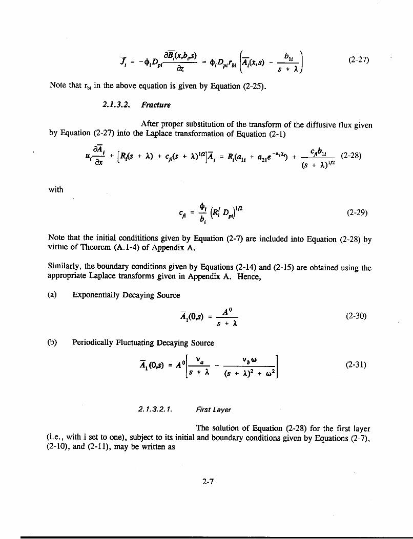
o= -(iDpi = iDprb (i S) - _ l) (2-27)
Note that rbi in the above equation is given by Equation (2-25).
2.1.3.2. Fracture
After proper substitution of the transform of the diffusive flux givenby Equation (2-27) into the Laplace transformation of Equation (2-1)
uf -f + [R1(s + A) + cfl(S + A)1f2]A = R1(a1, + a21e -eXd) + Cfibl, (2-28)ax ,(s + XL'2;j=R~li+a, S ;) 1t2
with
Cfii =b (ID/ Dpz) 1 2 (2-29)
Note that the initial condititions given by Equation (2-7) are included into Equation (2-28) byvirtue of Theorem (A. 1-4) of Appendix A.
Similarly, the boundary conditions given by Equations (2-14) and (2-15) are obtained using theappropriate Laplace transforms given in Appendix A. Hence,
(a) Exponentially Decaying Source
Ai(O's) = A (2-30)S +
(b) Periodically Fluctuating Decaying Source
A7(n = AO[ Va 1 (2-31)~ AS = s+A (s + A)2 + (,2J
2. 1.3.2. 1. First Layer
The solution of Equation (2-28) for the first layer(i.e., with i set to one), subject to its initial and boundary conditions given by Equations (2-7),(2-10), and (2-11), may be written as
2-7

where
Al(xs) = rFo - T1] e 411+ +j;
So = Al(Os)
3=Ti = Ff i (S)
j=1
4
Ti = Ef, (s)1=1j*2
(2-32)
(2-33a)
(2-33b)
(2-33c)
with
fliks) - RialiRa
f2i(s) = Rgrai - Pi
f3A(S) =
f 4,(XIs) = f2*(s) e ,xl
rai = R (s + X) + Cfi(S +
Pi = uialc
rd = r. (s + X)V2
(2-34a)
(2-34b)
(2-34c)
(2-34d)
and
(2-35a)
(2-35b)
(2-35c)
2-8

n = Li (2-35d)Ui
T~i xi (2-35e)U.
Note that subscript i refers to a typical layer and Xi given by Equation (2-8) corresponds to thedistance within the portion of the fracture network stretching between the exit face of layer i-Iand the location of the observation point in layer i.
2. 1.3.2.2. Second Layer
With the assumption that the upstream boundarycondition of the second layer will correspond to the prevailing concentration at the downstreamend of the first layer (see Equation (1-4)), we may write
A2(0,s) = A 1(L,,s) (2-36)
hence the solution of Equation (2-28), related to the second fracture layer, may be written as
A 2(xs) = (FO - F [.)e + r2 + (F1 - + 2(2-37)
2.1.3.2.3. Nth Layer
Applying successively the above approach to thesubsequent portions of the fracture layers, the solution of Equation (2-28) corresponding to thenth layer may be written as
An(xws) = [ro - Pi]e le I eFStan
(2-38)
+ , (FI.i - -r,.)e Hrnx e -rt In +i-2 j-i
Using the following notations
2-9

0~~~flfl = ~~~~~~~(2-39)i=M
n-l
m= Cf 1 1i + R.ii3 (2-40)i=m
n-l -
Bn(x~s) = e FMuIJ e FaIi = e -Y." + A) - O(s + A)I (2-41)i-r
the inverse Laplace transform of Equation (2-38) yielding the closed form solution of theconcentration of a typical species in the nth fracture layer is obtained by means of the varioustheorems and Laplace transforms reported in Table A of Appendix A. This may be written as
An(xt) = Fo(xt) - S Flii(xt) +
(2-42)
E F1 jV,(x~t) + F,,(x,t)i-2
The various components of the above equation correspond to
Fo (xt) = L-1 [FO gj,(xs)] (2-43a)
3F 'n(x, t) = S L -fj(s) *g~ (x s) (2-43b)
j-l
3Fi,,(xt) = FL- fj(s) gmm(s) + L 'f4 (xs) g,1 (xs) (2-43c)
j=1
J*2
3
F,(xt) = L -fj(s) + L -f4n(xs) (2-43d)J=1
jo2
where FO, fm,,(s), and g (x,s) are given by Equations (2-33a), (2-34), and (2-41) respectively.
2-10

The components of functions F01j(x,t), Flim,(x,t), F ^(x,t) and F.(x,t) are now given by:
(a) Exponentially Decaying Source
Fo (xt)= L-'[FPo g1 3 (xs)] = AOel e'ct [ 1 ] U(t - Y n) (2-44a)
(b) Periodically Fluctuating Source with Exponential Decay
FO(xt) =L - FO.g91 (xIS)I = Aee e[ ] -
(2-44b)
-. [E(t-y1̂ ,O~lica) - E(t Y 0 i@)]|U(t -Yd
The reader may refer to Appendix A, Equation (A.2-3) for a full definition of function E(-) .Note that the second member of the above equation, which includes a combination ofexponential and complementary error functions with complex arguments, has been shown toyield a real number (see Appendix B, Section B.3).
The inverse Laplace transforms of the the right hand side of Equations (2-43b), (2-43c) and (2-43d) are given by
L-l [fij(S) g"n(X'S)]
eroC[C (t _
[f ~~~~2L-1 [f2,(s).gmn(xs)] = Y
erf[P#(t -
= eAt aU, exR[ 0 xp Ri (t - Y.)|-
Ynl 2 (t ymn)' 1 U(t-y,,)
' (-1) e -A a 1 exr.iom, + 013(t -Ym)]
y)12 + ., [U]
Y, ~2 (t -Y.)Ut-,)
(2-45a)
(2-45b)
2-11

L-1 [f31(s) gmn(xs)] = e-tbiferfc( 2(t - ex n P[R O
(2-45c)
exp[(C) (t - y.. erfc Ri (t - y +n 2 ' j U(t-ym)
Ll[f4,(xs) g,,(xs)] = e lxi L-1 [f2,(s) gm.(xIs)]
L 1 [f1i(s)] = e 4taliexp[(pfl( )tjercl'i2
(2-45d)
(2-46a)
L l[f4i(XIS)] =2E (-ly
j - I
a2je ~e ( - P)t erfc(Pit 1t2) (2-46b)
(2-46c)L 3i(S) = e -blib1 - expf(.ltj t erfift
with
= 2R(. ) Ri(2-47)
and
2-12

Pi = c _l qi (2-48a)2R, 2
P2i = Cfl + qj (2-48b)2R1 2
Note that Oli and 02i have dimensions of t-112.
Grouping the components of Fj! (xft), Finn(xt), and F.(x,t), one may then write
F'imn(xt) = H,,,(xt) + ,Hj(xt) (2-49)
Fj,,(xt) = 1Hj,,(xat) + e-' lHA, (xt) (2-50)
where
1H,,,(x,t) = e b|lierfc [2(t + (a,, - bli)expf R.
(2-51)
exp[(J R 2t j Y u[)(c -| + (t 2 +(,,1 ] u -Y)
and
2-13

2 aPf3.22H,.,(xOt) = e E (-ly ex_ p [ Pj_ + P -(t - yj]-
(2-52)
[rfi -Pi, R)12Y. 2(t ) 1.> mY
2 a ,,j .e n Xp2tF n(xt) = P (-1)' 2r e fC(pit112) +
(2-53)
e~A'bl, + al, - ln)exp trn *erfCI f" tin]]
Note that the evaluation of expressions involving products of exponential and complementaryerror functions are presented in Appendix B.
2.1.3.3. Rock Matrix
Substitution of Equation (2-38) in Equation (2-24) gives the Laplacetransform solution of the concentration in the nth layer of the rock matrix
B,(x,z,s) = [o- P Il e - 'rn + r(z-b) II e -tan, +i-i
Y (Fi l -F'i)e -[r.. . + r&,(b,-] JJ e + (2-54)i-2 j=a
F-e rb.(z-b^) + 1 (1 - ("))
The inverse Laplace transform of the above equation yielding the closed form solution of theconcentration in the nth layer of the rock matrix is then obtained by means of the varioustheorems and Laplace transforms reported in Appendix A. This may be written as
2-14

B^(xzt) = G.l (xz,t) - S G',,(xz,t) +i-i
(2-55)nx G i-,(xz,t) + G,(x~z,t)i-2
The components of functions Gol(x, z, t), G(,,/ (x,z,t) , Gin(x, z, t) and G.(x, z, t) are nowgiven by:
(a) Exponentially Decaying Source
Go (x,z,t) = A e t erfc [ 1 (2-56a)[2(t - Ut
(b) Periodically Fluctuating Source with Exponential Decay
G 0 (xzt)=L-F B.gj(x,s)| = AOe-1vterfcf Y (
(t y 1.) ~(2-56b)
b [E(t-y fO/ i(,) - E(t-y In O', ,-ic)] U(t - Yln)
where function E(*) is given in Appendix A, Equation (A.2-3).
G' (x,z,t) = IH ' (x,z,t) + 2H', (x,z,t) (2-57a)
Gi,,,(x,z,t) = 1H',,(xzt) + e 6Lxa2H', ,(xz,t) (2-57b)
where
2-15
H O ~e t b e rfc[ . 1 12 1 )ep af]n(xt) = + (ali - b_)R;
(2-58)
expf(R)2(t - Y)ie rf l (t - y.)1 2 + o 1 t2Il -YU(t )Ri ~~2 (t
2 Hl,,,(xz,t) = c E ("expct3 0/ + I3 (t -
(2-59)
0'erfcM 0,(t - y /2 + - jU(t -Y-n)
2~~~~~~~~~~~~,/
F,(xzt) = e;tj (-l)i in +b)]
erfc cit(z)2) + m + e -tA bl + (aln - b1n) exp (z - b3) c1- (2-60)
eRp[(, ) |eMfR[t12 + 2t1123]
',/,| = 0 + cm (z - b) (2-61)
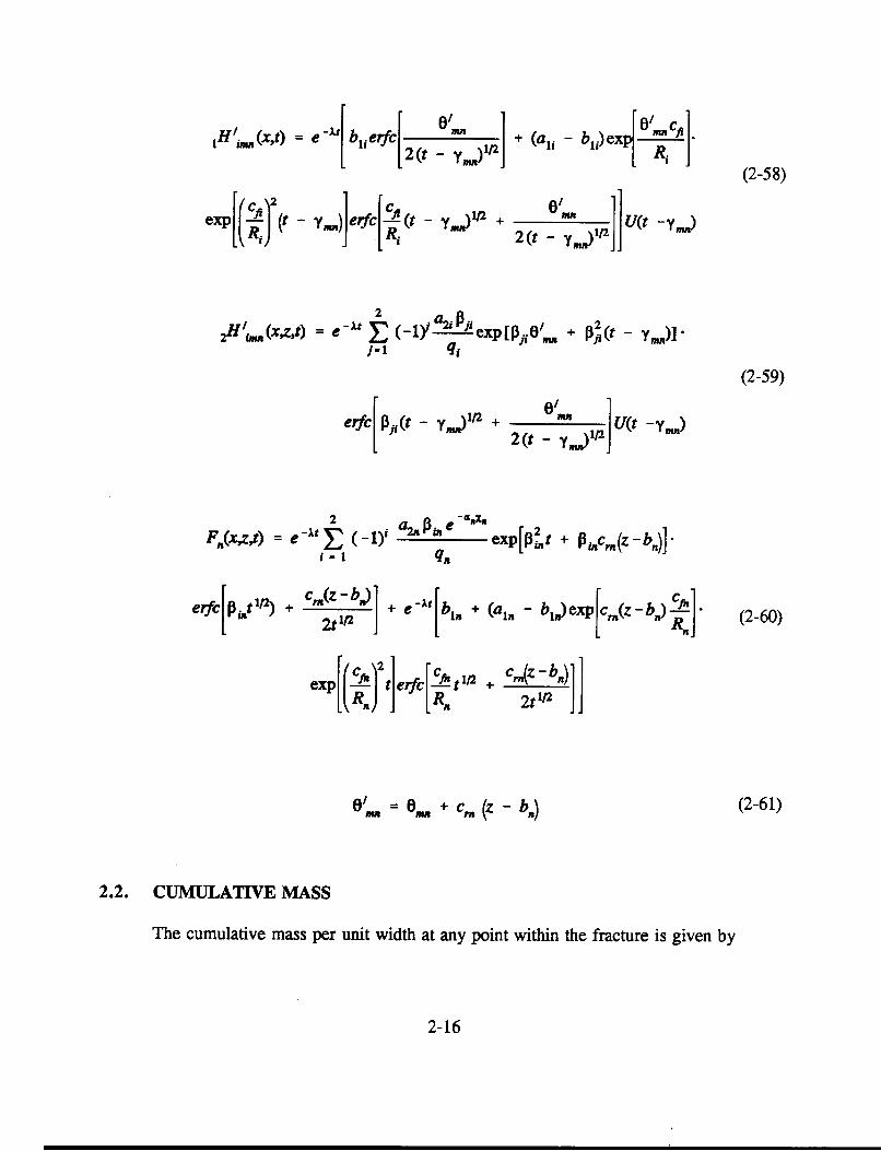
2.2. CUMULATIVE MASS
The cumulative mass per unit width at any point within the fracture is given by
2-16

tn
M(xt) = fq,12bnAn(xr)dr = q,,2b,, QOI (Xt) Q in(xst)1=1 (2-62)
+ Qi li,(Xlt) + Qn(xlt)|i=2
where A.(x,t) the concentration in the fracture is given by Equation (2-42). In the aboveequation the components of functions Qol0 (x,t), Q'j(x,t), Qin(x,t) and Q(x,t) are evaluated basedon the various integrals derived in Appendix C and are given by
(a) Exponentially Decaying Source
t0
QO(xt) = fF0 @(s)dt = AOI(t,X, eyn) U(t - Y'.) (2-63a)Q~~t iA,2YLX
(b) Periodically Fluctuating Source with Exponential Decay
t
QO (x~t) = fFO0 (T)&d =Y1. (2-63b)
A [VaIl(t0,, 2 'Yn) - Vbo I n14 s '.) U(t-y )
Ql (x,t) = fFi ,(x,r)di = 1QII..(xlt) + 2 Qiann(xt) (2-64a)
Y_
Qimn(Xlt) = f Fin(x,-r)dr = 1QL(xt) + e "i 2QI(xt) (2-64b)YM
where
2-17
unn(rst) = tin( s= s2,n01Q 'n(xv) = f IHi.(x,,r)dT = [b11Ii(t,;L'- 'Ym)
(2-65)
+ (a1, - bl')exp[f~(0 - Cfly I ) - nft mnU(t - Yn)
2Q'i, (xt) 2 Hin(x,,r) dT = E (- ly a expf P3f(e3mn Pi Y..) ]J-1 q
(2-66)
I 2 (t,( i - AX), pi2 'Y U(t - Ym.)
t
Q.(xt) = f F.(xt)0
- O -li a 4 e -a^ I3(0,t,(p2^ )p"= 2 ( inI~~= 1 1,.
(2-67)
+ (1 - e') + (a,, - bln)13 (Rt,((fŽ) C;L , fnRn)
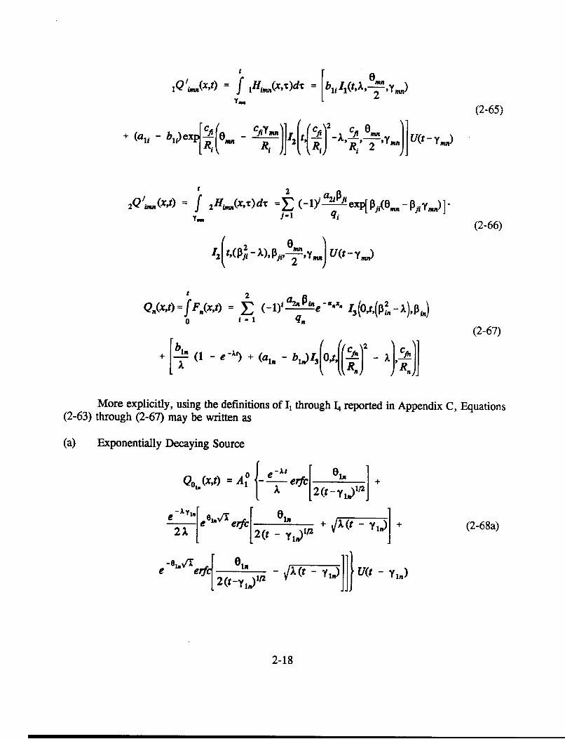
More explicitly, using the definitions of I1 through 14 reported in Appendix C, Equations(2-63) through (2-67) may be written as
(a) Exponentially Decaying Source
Q,(xVt) = Al ( A e4c r
eA |t°XyeC|2t +lv/-,% elmt ~2+T eoi r erfc[ Ol + i)]+(2-68a)
e 0 c lL2(t-yl,)'/
- (- Yn)jj} U(t - Y 1.)
2-18
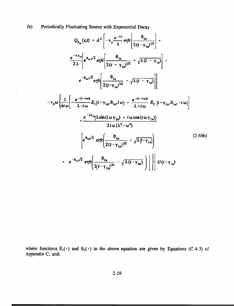
(b) Periodically Fluctuating Source with Exponential Decay
Q 0'(xt) - A a I 2 t - +
e ee|.V/' erfc In - + - +2 [ 2(t - yd12 V t 1
-e,31 0 1e er in
1 2(t-yl,,)1
- Vo4W - eEi E (t-Y 1m,' 1 ,i Ci)
- ,t Yin)]]
e -(A + i (OE2 (t- 1 0Yn -ica)
I +i~~~~n'in j
e - Y'(A sin (i ( Y 1..) + i cos (i c Y in))+ -
[ej'V - (la + 0
ie ' erfti in)Y +XtY
(2-68b)
+ e 1°r derf| 1^t 4 - I/ATU"11)-_y______ I ] I U(t-Yin)
where functions E 1(-) and E 2(.) in the above equation are given by Equations (C.4-3) ofAppendix C, and:
2-19

1Q'im(Xst) = bui{e e mm +
2A ,1 e e + VI(t Y.) j+e 8mO.lle lfr[
12(t-yl)"2
+ (aXy,, - __ __t (
2 fc2 Ri MR2~~ 2 (t -ym ,,,
- Ft - Y) U(t- y)
_Aid) Cf2 AAJ&Jt
I
V+ (t - y,.,)12 ] (2-69)
+ VA(t - y, + 1) -
e - 4 rerfc[2 (t - y.|)"
V�- Y� cM) fi
Rij- 1 U(t-y,,,)
2-20

2 Q'UR(Xlt) =
P;, - A
exp(- A y o.@
2(P; - A)[
i-l(-lYa2, PAi f exp[f P,(OJ,,,1 - PiY)
qi
erfc p(t - yJ.)A 2 + _ )11n ]
4- Xt- Ymnl j(T + 1 - (2-70)
e erfq|2(t- ym,,) U
- VTU-- -YM5 DiiFl
I U(t-y.)
Q,,(x,t) = EJ-1
(-ly e -axxxqn
1 [e('1)terc(p,,,it) +(p;2 - A)
Pi e r (AXt) /2]
+ -l. - C_ -A + (a,, - bl,
e1fcr 2t1+1
e6CR~t +-R.
- 1
- I - (2-71)
I{(X t)1/2]
..
2-21

Note that when the exponential term in the model describing the initial concentration distributionin the fracture (see Equation (2-7)) is taken into account, overflow problems are likely to beencountered when the value of the time parameter becomes excessively large. This state ofaffairs is inherent to the presence of parameter hij (see, for example, Equation (2-52)), whichby virtue of being negative (i.e., when subscript i corresponds to 1, see Equation (2-48a)), tendsto freeze the complementary function at a constant value of approximately 2 (i.e., when itsargument becomes less than or equal to -3), whilst the exponential term will increase positivelywith increasing values of time. To mitigate the incumbent overflow problem, the solution isoptimized through an iterative process intended to estimate an acceptable upper limit for themagnitude of the exponential argument. Consequently, exponential terms witnessing j31j in theirlist of arguments are ignored (i.e., set automatically to zero) when the preset limit is exceeded.Computationally, this is achieved after initializing the significant absolute limit of the exponentialargument, initially to a value corresponding to 30, the latter affecting exclusively the specificcomponents of the solutions which include parameter fllj . The computation is reiterated afterhalving the value of the exponential argument, and the absolute relative error in the computedresults is subsequently estimated. This process is continued until when, in two successiveiterations, the preset convergence criteria (i.e., 1 % relative error) is said to be satisfied. Forthe test cases reported herein a maximum of three iterations were proven sufficient to providean optimized value of the exponential argument and yield a highly accurate solution.
2.3. DISCUSSIONS OF RESULTS
The analytical solutions presented in this section of the report were verified bycomparison with three approximate methods of Laplace inversion integral as proposed by Talbot(1979), Durbin (1974), as modified by Piessens and Huysmans (1984) and Stefhest (1970). Allthree methods apply to the case where the source term corresponds to a continuous exponentiallydecaying one, in which instance the required inversion of the Laplace transform is strictlyconfined to the real domain. However, when a periodically fluctuating and decaying source termis adopted, then only the first two of these methods are useful for evaluating the Laplacetransform inversion in the complex domain. Note that in the case of Stefhest's algorithm, 36summation points were found to produce almost oscillation-free solutions.
As far as the calculation of the analytical solution related to the cumulative mass (i.e.,the time integrated solution of the concentration at a typical point along the longitudinal axis ofthe fracture) is concerned, this is performed by numerically integrating solutions of the Laplace-transformed equation of the concentration in the fracture. This integration is performed usinga composite Gauss-Legendre quadrature scheme, where 40 integration points were foundadequate to yield a convergent quadrature for the investigated test cases.
The two test cases reported subsequently refer to the one-dimensional transport of tworadionuclides: Np-237 (i.e., long half-life) and Cm-245 (short half-life), in a heterogeneoussaturated fractured rock system composed of five layers (the last extending to infinity), withpiecewise constant parameters. In the first test case, the imposed source term corresponds toan exponentially decaying function (see Equation (2-14)). This is substituted by a periodically
2-22

fluctuating and decaying one (see Equation (2-15)) in the second, respectively. In both cases,the steady flow rate of water per unit width of fracture corresponds to 0.1 m2/yr. Two types ofsolute release modes at the source were investigated namely: step and band. Note that the flowdomain in both fracture and rock layers are assigned non-zero initial concentrations (seeEquations (2-7) and (2-9)).
2.3.1. Case 1 Results
This test case examines the spatial and temporal variation of the concentrationof Np-237, as well as the cumulative release of mass from the fracture. In addition, the spatialvariation of the concentration in the rock matrix is also investigated. The input data pertainingto this test case is presented in Table 2-1.
Figure 2-2(a) shows the spatial relative concentration profiles of Np-237calculated in the fracture layers at simulation times of 103, 5xlo3 and 5x10⁴ years. Acomparison of our results with the ones obtained from the three numerical inversion algorithms(see Tables 2-2(a) through 2-2(c)) show that these are in excellent agreement. Note that in thistest case, the observation times were selected in a manner to allow an evaluation of the accuracyof our solution for both release modes of the radionuclide at the source, it may be added thatin the case of the intermediate observation time, the source strength is reduced by half from itsoriginal value (see Equation (2-17)).
Figure 2-2(b) shows the temporal relative concentration of Np-237 observed inthe fracture at three different observation points: 100, 200, and 500 meters downstream fromthe source, located in the second, third and fifth layer, respectively, for a band release. Up tothe leaching time of 5x10³ years, the shape of the profiles bears a close similarity with those ofa step release. Past the leaching time, the relative concentrations profiles show a rapid changeof their gradient from positive to negative and concentrations decrease with time to a value lyingwithin close range to the initial concentrations of the various fracture layers of interest. Acomparison of our results with the three numerical ones (see Tables 2-3(a) through 2-3(c)) showthat with the exception of a portion of the results yielded by Talbot's solution, these are inexcellent agreement. Note that in this instance, the adoption of three recommended' values ofthe constants required by Talbot's algorithm, seems to have restricted the accuracy of the latterto simulation times greater than 30, 80 and 100 years. Therefore, it appears that the threeconstants in Talbot's algorithm seem to be correlated with the independent variables, renderingtheir selection problem dependent.
Figure 2-2(c) depicts the time-dependent evolution of the cumulative mass (perunit width of the fracture) profile at three different observation points in the fracture as in theprevious example. Because of its computational viability Steftest's algorithm is selected fromthis point on as the benchmark. A comparison of our analytical solution results with those
l D. Hodgkinson, personal communication.
2-23

yielded by Stefhest's solution (see Tables 2-4(a) through 2-4(c)) indicates excellent agreement.Note that all three profiles tend to become asymptotic to three specific values of the cumulativemass namely, 4.903 x10², 4.7 x10², and 4.309 x10² (UA/m)2. The latter may be easilycomputed from Equation (2-62) after setting the value of the independent variable t equal toinfinity.
Figure 2-2(d) shows the concentration profiles in the rock matrix at threepositions downstream from the source (i.e., x = lOOm, 200m, and 500m) for a step release.Comparison of our analytical results against those yielded by the Stefhest's solution method (seeTables 2-5(a) through 2-5(c)) indicate an excellent agreement. Note that at their downstreamend, all three profiles tend to become asymptotic to a concentration value slightly in excess ofthe residual concentration prevailing in their respective layers.
Figure 2-2(e) shows the concentration profiles in the rock matrix at threepositions downstream from the source (i.e., x = lOOm, 200m, and 500m) and for a simulationtime of 5x10⁴ years, for a band release with a leaching time corresponding to 5x10³ years. Pastthe leaching time, the contaminant in a typical rock layer close to the source would begin toexhibit a higher concentration than in the fracture, which would then initiate its diffusion backinto the fracture. Indeed a quick reference to Figure 2-2(e) shows that the gradient of theconcentration profiles at the fracture rock interface tends to decrease with increasing distancesfrom the source. As in the preceding case, results reported in Tables 2-6(a) through 2-6(c) showexcellent agreement between the analytical and the numerical solutions.
2 UA: Arbitrary Units of Activity/meter.
1-
2-24

Table 2-1. INPUT PARAMETERSSOURCE
FOR CASE 1 EXPONENTIALLY DECAYING
SPECIES Np-237
2.3 x 10⁶ yr
Release Mode:StepBand Leaching Time
NA5 x 103 yr
A° 1.0
Q 0.1 (m 2 /yr)
VA NA
Vb NA
NA
1 50.0 5.OE-03 10.0 0.01
2 75.0 4.OE-03 12.5 0.008
3 100.0 3.OE-03 16.666 0.006
4 150.0 2.OE-03 25.0 0.004
5 cO 1.5E-03 33.333 0.002
1 2.0 0.01 5.OE-03 0.5
2 2.3 0.02 8.OE-03 0.6978
3 2.6 0.06 2.7E-02 1.158
4 2.65 0.05 1.OE-02 1.059
5 2.7 0.03 3.OE-03 0.741
2-25

Table 2-1. INPUT PARAMETERS FOR CASE 1 EXPONENTIALLY DECAYINGSOURCE (Continued)
LAYER al . a mWY _ ___1 1.50E-04 -0.50E-04 0.02 1.OOE-05
2 2.OOE-04 -0.25E-05 0.02 1.75E-05
3 1.75E-04 -0.20E-05 0.02 1.25E-05
4 2.OOE-04 -0. 15E-05 0.02 1.05E-05
5 1.50E-04 -0.20E-05 0.02 1.05E-05
. (arbitrary units of activity/L3)
2-26

M M s - - - - : m a g I M M M V M IM
10o
10-,4:
a)
r 10-2
cU-CC0
.T l o-,CCD)C000) 1 -
Cr
t'j
10-6 L
1-1100 101 102 13 104
Distance, x(m)
Figure 2-2(a). Relative concentration of Np-237 vs. distance in the fracture at different times t = 1,000, 5,000, and50,000 years (Exponentially decaying source and step and band release).

Table 2-2(a). CASE 1 RESULTS: CONCENTRATION OF Np-237 IN THE FRACTUREAT TIME t = 1,000 YEARS (EXPONENTIALLY DECAYING SOURCE AND STEPRELEASE MODE)
DISTANCE (m) M CULTFRASTEFHEST TALBOT DURBIN
1 .OOOE-O11.500E-O12.OOOE-013.OOOE-O14.OOOE-O15.OOOE-O16.OOOE-O17.OOOE-O18.OOOE-O19.OOOE-O11 .OOOE+OO1.500E+OO2.OOOE+OO3.OOOE+OO4.OOOE+OO5.OOOE+OO6.OOOE+OO7.OOOE+OO8.OOOE+OO9.OOOE+OO1.OOOE+O11.500E+O12.OOOE+O13.OOOE+O14.OOOE+O15.OOOE+O16.OOOE+O17.OOOE+O18.OOOE+O19.OOOE+O11.OOOE+021.500E+022.OOOE+023.OOOE+024.OOOE+025.OOOE+02
9.993E-O19.992E-O19.990E-O19.986E-O19.983E-O19.979E-O19.976E-O19.972E-O19.968E-O19.965E-O19.961E-O19.943E-O19.926E-O19.890E-O19.854E-O19.819E-O19.783E-O19.747E-O19.711E-O19.676E-019.640E-O19.461E-O19.283E-O18.927E-O18.572E-O18.219E-O17.550E-O17.061E-O16.558E-O16.056E-O15.564E-O12.491E-O15.308E-021.400E-033.744E-051.409E-05
9.993E-O19.992E-O19.990E-O19.986E-O19.983E-O19.979E-O19.976E-O19.972E-O19.968E-O19.965E-O19.961E-O19.943E-O19.926E-O19.890E-O19.854E-O19.819E-O19.783E-O19.747E-O19.71 lE-Ol9.676E-O19.640E-O19.462E-O19.283E-O18.927E-O18.572E-O18.219E-O17.662E-O17.116E-O16.582E-O16.064E-O15.564E-O12.490E-O15.308E-021.400E-033.761E-051.41 1E-05
9.993E-O19.992E-O19.990E-O19.986E-O19.983E-019.979E-O19.976E-O19.972E-O19.968E-O19.965E-O19.961E-O19.943E-O19.926E-O19.890E-O19.854E-O19.819E-O19.783E-O19.747E-O19.71 lE-Ol9.676E-O19.640E-O19.462E-O19.283E-O18.927E-O18.572E-O18.219E-O17.662E-O17.116E-O16.582E-O16.064E-O15.564E-O12.490E-O15.308E-021.400E-033.761E-051.41 1E-05
9.993E-O19.992E-O19.990E-O19.986E-O19.983E-O19.979E-O19.976E-O19.972E-O19.968E-O19.965E-O19.961E-O19.943E-O19.926E-O19.890E-O19.854E-O19.819E-O19.783E-O19.747E-O19.71 lE-Ol9.676E-O19.640E-O19.462E-O19.283E-O18.927E-O18.572E-O18.219E-O17.662E-O17.116E-O16.582E-O16.064E-O15.564E-O12.490E-O15.308E-021.400E-033.761E-051.413E-05
2-28
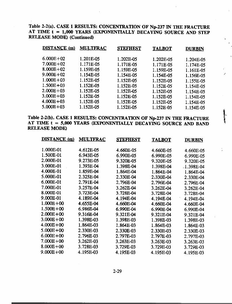
Table 2-2(a). CASE 1 RESULTS: CONCENTRATION OF Np-237 IN THE FRACTUREAT TIME t = 1,000 YEARS (EXPONENTIALLY DECAYING SOURCE AND STEPRELEASE MODE) (Continued)
DISTANCE (m) MULTFRAC STEFHEST TALBOT DURBIN
6.OOOE+027.OOOE+028.OOOE+029.OOOE+021.OOOE+031.500E+032.OOOE+033.OOOE+034.OOOE+035.OOOE+03
1.201E-051. 171E-051. 159E-051. 154E-051. 152E-051. 152E-051. 152E-051.152E-051. 152E-051. 152E-05
1.202E-051. 171E-051. 159E-051.154E-051. 152E-051.152E-051. 152E-051. 152E-051. 152E-051. 152E-05
1.202E-051. 171E-051. 159E-051. 154E-051. 152E-051. 152E-051. 152E-051. 152E-051. 152E-051. 152E-05
1.204E-051. 174E-051. 161E-051. 156E-051. 155E-051. 154E-051. 154E-051. 154E-051. 154E-051. 154E-05
Table 2-2(b). CASE 1 RESULTS: CONCENTRATION OF Np-237 IN THE FRACTUREAT TIME t = 5,000 YEARS (EXPONENTIALLY DECAYING SOURCE AND BANDRELEASE MODE)
DISTANCE (m) MULTFRAC STEFHEST TALBOT DURBIN
1.OOOE-011.500E-012.OOOE-013.OOOE-014.OOOE-015.OOOE-016.OOOE-017.OOOE-018.OOOE-019.000E-011.OOOE+001.500E+002.OOOE+003.OOOE+004.OOOE+005.OOOE+006.OOOE+007.OOOE+008.OOOE+009.OOOE+00
4.612E-056.943E-059.273E-051.393E-041.859E-042.325E-042.791E-043.257E-043.723E-044.189E-044.655E-046.986E-049.316E-041.398E-031.864E-032.330E-032.796E-033.262E-033.728E-034.195E-03
4.660E-056.990E-059.320E-051.398E-041.864E-042.330E-042.796E-043.262E-043.728E-044.194E-044.660E-046.990E-049.321E-041.398E-031.864E-032.330E-032.797E-033.263E-033.729E-034.195E-03
4.660E-056.990E-059.320E-051.398E-041.864E-042 330E-042.796E-043.262E-043.728E-044.194E-044.660E-046.990E-049.321E-041.398E-031.864E-032.330E-032.797E-033.263E-033.729E-034.195E-03
4.660E-056.990E-059.320E-051.398E-041.864E-042.330E-042.796E-043.262E-043.728E-044.194E-044.660E-046.990E-049.321E-041.398E-031. 864E-032.330E-032.797E-033.263E-033.729E-034.195E-03
2-29

Table 2-2(b). CASE 1 RESULTS: CONCENTRATION OF Np-237 IN THE FRACTUREAT TIME t = 5,000 YEARS (EXPONENTIALLY DECAYING SOURCE AND BANDRELEASE MODE) (Continued)
DISTANCE (m) MULTFRAC STEFHEST TALBOT DURBIN
1.OOOE+011.500E+012.OOOE+013.OOOE+014.OOOE+015.OOOE+016.OOOE+017.OOOE+018.OOOE+019.OOOE+011.OOOE+021.500E+022.OOOE+023.OOOE+024.OOOE+025.OOOE+026.OOOE+027.OOOE+028.OOOE+029.OOOE+021.OOOE+031.500E+032.OOOE+033.OOOE+034.OOOE+035.OOOE+03
4.661E-036.992E-039.322E-031.398E-021.863E-022.327E-023.064E-023.796E-024.520E-025.234E-025.938E-021.080E-011.525E-011.642E-011.352E-011.135E-019.129E-027.056E-025.256E-023.784E-022.638E-022.836E-031.703E-041.087E-051.079E-051.079E-05
4.661E-036.992E-039.323E-031.398E-021. 863E-022.327E-023.064E-023.796E-024.520E-025.234E-025.938E-021.080E-011.525E-011.642E-011.352E-011.135E-019.129E-027.056E-025.256E-023.784E-022.638E-022.836E-031.703E-041.087E-051.079E-051.079E-05
4.661E-036.992E-039.323E-031.398E-021.863E-022.327E-023.064E-023.796E-024.520E-025.234E-025.938E-021.080E-011.525E-011.642E-011.352E-011. 135E-019.129E-027.056E-025.256E-023.784E-022.638E-022.836E-031.703E-041.087E-051.079E-051.079E-05
4.661E-036.992E-039.323E-031.398E-021. 863E-022.327E-023.064E-023.796E-024.520E-025.234E-025.938E-021.080E-011.525E-011.642E-011.352E-011.135E-019.129E-027.056E-025.257E-023.784E-022.638E-022.837E-031.702E-041.089E-051.081E-051.081E-05
TABLE 2-2(c). CASE 1 RESULTS: CONCENTRATION OF Np-237 IN THE FRACTUREAT TIME t = 50,000 YEARS (EXPONENTIALLY DECAYING SOURCE AND STEPRELEASE MODE)
DISTANCE (m) MULTFRAC STEHEST TALBOT
1.OOOE-011.500E-012.OOOE-013.OOOE-014.OOOE-01
2.479E-063.824E-065.169E-067.859E-061.055E-05
2.689E-064.034E-065.379E-068.068E-061.076E-05
2.689E-064.034E-065.379E-068.068E-061.076E-05
2.689E-064.034E-065.379E-068.068E-061.076E-05
2-30

Table 2-2(c). CASE 1 RESULTS: CONCENTRATION OF Np-237 IN THE FRACTUREAT TIME t = 50,000 YEARS (EXPONENTIALLY DECAYING SOURCE AND STEPRELEASE MODE) (Continued)
DISTANCE (m) MULTFRAC STEFIEST TALBOT DURBIN
5.OOOE-016.OOOE-017.OOOE-O18.OOOE-019.OOOE-011.OOOE+0O1.500E+002.OOOE+003.OOOE+004.OOOE+005.000E+006.000E+007.OOOE+OO8.OOOE+009.OOOE+OO1.OOOE+011.500E+012.OOOE+O13.OOOE+O14.OOOE+015.OOOE+016.OOOE+O17.OOOE+018.000E+019.OOOE+O11.OOOE+021.500E+022.OOOE+023.OOOE+024.OOOE+025.OOOE+026.OOOE+027.OOOE+028.OOOE+029.OOOE+021.OOOE+031.500E+032.OOOE+03
1.324E-051.593E-051. 862E-052.131E-052.400E-052.669E-054.013E-055.358E-058.048E-051.074E-041.343E-041.612E-041.881E-042.150E-042.419E-042.688E-044.032E-045.377E-048.066E-041.075E-031.344E-031.774E-032.203E-032.632E-033.060E-033.486E-036.700E-031.082E-021.656E-022.018E-022.174E-022.300E-022.398E-022.467E-022.508E-022.521E-022.248E-021.642E-02
1.345E-051.614E-051.883E-052.15 lE-052.420E-052.689E-054.034E-055.379E-058.068E-051.076E-041.345E-041.614E-041.883E-042.152E-042.420E-042.689E-044.034E-045.379E-048.068E-041.076E-031.344E-031.774E-032.203E-032.632E-033.060E-033.486E-036.700E-031.082E-021.656E-022.018E-022.174E-022.300E-022.398E-022.467E-022.508E-022.521E-022.248E-021.642E-02
1.345E-051.614E-051. 883E-052.151E-052.420E-052.689E-054.034E-055.379E-058.068E-051.076E-041.345E-041.614E-041.883E-042.152E-042.420E-042.689E-044.034E-045.379E-048.068E-041.076E-031.344E-031.774E-032.203E-032.632E-033.060E-033.486E-036.700E-031.082E-021.656E-022.018E-022.174E-022.300E-022.398E-022.467E-022.508E-022.521E-022.248E-021.642E-02
1.345E-051.614E-051. 883E-052.151E-052.420E-052.689E-054.034E-055.379E-058.068E-051.076E-041.345E-041.614E-041.883E-042.152E-042.420E-042.689E-044.034E-045.379E-048.068E-041.076E-031.344E-031.774E-032.203E-032.632E-033.060E-033.486E-036.700E-031.082E-021.656E-022.018E-022.174E-022.300E-022.398E-022.467E-022.508E-022.521E-022.248E-021.642E-02
2-31

Table 2-2(c). CASE 1 RESULTS: CONCENTRATION OF Np-237 IN THE FRACTUREAT TIME t = 50,000 YEARS (EXPONENTIALLY DECAYING SOURCE AND STEPRELEASE MODE) (Continued)
DISTANCE (m) MULTFRAC STEFHEST TALBOT DURBIN
3.OOOE+034.OOOE+035.000E+03
5.3 11E-039.475E-041.046E-04
5.31 IE-039.475E-041.046E-04
5.3 11E-039.475E-041.046E-04
5.31 1E-039.474E-041.046E-04
2-32

mm- m m - -- - m - -mm
100
10-'
a o-
ZC 10-2.5
18 1 0-3
10-
1 -5 _
10- 100 101 102 10 3104 10 5
Time, t(yr)106
Figure 2-2(b). Relative concentration of Np-237 in the fracture vs. time at different positions x = 100 meters, 200meters, and 500 meters (Exponentially decaying source).

Table 2-3(a). CASE 1 RESULTS: CONCENTRATION OF Np-237 IN THE FRACTURELAYER 2, AT DISTANCE x = 100 METERS (EXPONENTIALLY DECAYING SOURCEAND STEP RELEASE MODE)
TIME t(yr) MULTFRAC STEFHEST TALBOT DURBIN
1.OOOE-011.500E-012.000E-013.000E-014.000E-015.000E-016.000E-017.000E-018.000E-019.000E-011.000E+001.500E+002.000E+003.000E+004.000E+005.000E+006.000E+007.000E+008.OOOE+009.000E+001.000E+011.500E+012.000E+013.000E+014.000E+015.000E+016.000E+017.000E+018.000E+019.000E+011.000E+021.500E+022.000E+023.000E+024.000E+025.000E+026.000E+027.000E+02
1.370E-041.278E-041.209E-041.109E-041.037E-049.806E-059.353E-058.975E-058.652E-058.371E-058.124E-057.215E-056.617E-055.850E-055.362E-055.016E-054.753E-054.546E-054.376E-054.234E-054.113E-053.694E-053.440E-053.129E-054.396E-055.396E-042.886E-037.987E-031.580E-022.580E-023.739E-021.042E-011.682E-012.702E-013.443E-014.003E-014.444E-014.800E-01
1.370E-041.278E-041.209E-041.109E-041.037E-049.806E-059.353E-058.975E-058.652E-058.371E-058.124E-057.215E-056.617E-055.850E-055.362E-055.016E-054.753E-054.546E-054.376E-054.234E-054.113E-053.694E-053.439E-053.111E-054.359E-055.394E-042.885E-037.987E-031.580E-022.580E-023.739E-021.042E-011.682E-012.702E-013.443E-014.003E-014.444E-014.800E-01
3.453+248-1.309+258-1.006+263-1.457+232-3.245+2662.308+2351.153+2538.592+2132.367+2431.139+213-1.166+2541.420+223-3.639+234-1.693+237-3.822+167-1.900+125-1. 166E+973.444+168-5.676+1361.595+112-5.187E+937.614E+344;816E+053.122E-054.372E-055.392E-042.885E-037.987E-031.580E-022.580E-023.739E-021.042E-011.682E-012.702E-013.443E-014.003E-014.444E-014.800E-01
1.370E-041.278E-041.209E-041.109E-041.037E-049.807E-059.354E-058.976E-058.653E-058.372E-058.125E-057.216E-056.618E-055.848E-055.360E-055.014E-054.752E-054.544E-054.375E-054.232E-05
-4.111E-053.693E-053.439E-053.131E-054.373E-055.389E-042.885E-037.987E-031.580E-022.580E-023.739E-021.042E-011.682E-012.702E-013.443E-014.003E-014.444E-014.800E-01
2-34

Table 2-3(a). CASE 1 RESULTS: CONCENTRATION OF Np-237 IN THE FRACTURELAYER 2, AT DISTANCE x = 100 METERS (EXPONENTIALLY DECAYING SOURCEAND STEP RELEASE MODE) (Continued)
MULTFRAC STEFREST TALBOT DURBIN
8.OOOE+029.OOOE+021.OOOE+031.500E+032.OOOE+033.OOOE+034.OOOE+035.OOOE+036.OOOE+037.OOOE+038.OOOE+039.OOOE+031.OOOE+041.500E+042.OOOE+043.OOOE+044.OOOE+045.OOOE+046.OOOE+047.OOOE+048.OOOE+049.OOOE+041.OOOE+051.500E+052.OOOE+053.OOOE+054.OOOE+055.OOOE+056.OOOE+057.OOOE+058.OOOE+059.OOOE+051.OOOE+06
5.097E-O15.348E-O15.564E-016.322E-O16.789E-017.355E-017.697E-017.932E-012.550E-O11.462E-O11.005E-O17.528E-025.938E-022.650E-021.583E-027.972E-034.986E-033.486E-032.610E-032.046E-031.658E-031.378E-031. 168E-036.188E-043.936E-042.067E-041.300E-049.01 lE-056.647E-055.116E-054.063E-053.304E-052.738E-05
5.097E-015.348E-015.564E-016.322E-016.789E-017.355E-017.697E-017.932E-012.550E-011.462E-O11.005E-017.528E-025.938E-022.650E-021.583E-027.972E-034.986E-033.486E-032.610E-032.046E-031.658E-031.378E-031. 168E-036.188E-043.936E-042.067E-041.300E-049.013E-056.649E-055.118E-054.064E-053.305E-052.739E-05
5.097E-O15.348E-015.564E-016.322E-O16.789E-017.355E-O17.697E-O17.932E-O12.550E-011.462E-011 .005E-017.528E-025.938E-022.650E-021.583E-027.972E-034.986E-033.486E-032.610E-032.046E-031.658E-031.378E-031. 168E-036.188E-043.936E-042.067E-041.300E-049.013E-056.649E-055.118E-054.064E-053.305E-052.739E-05
5.097E-015.348E-015.564E-o16.322E-O16.789E-017.355E-017.697E-O17.932E-O12.550E-011.462E-011.005E-O17.528E-025.938E-022.650E-021.583E-027.972E-034.986E-033.486E-032.610E-032.046E-031.658E-031.378E-031. 168E-036.188E-043.936E-042.067E-041.300E-049.013E-056.649E-055.118E-054.064E-053.305E-052.739E-05
2-35
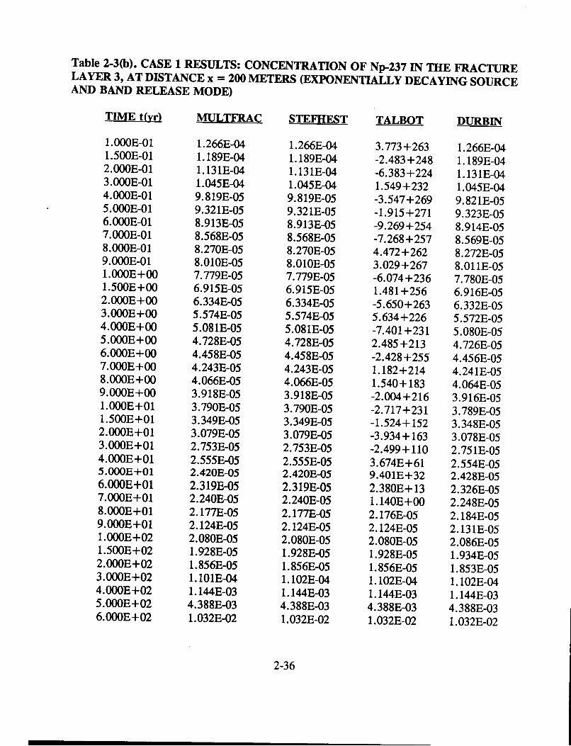
Table 2-3(b). CASE 1 RESULTS: CONCENTRATION OF Np-237 IN THE FRACTURELAYER 3, AT DISTANCE x = 200 METERS (EXPONENTIALLY DECAYING SOURCEAND BAND RELEASE MODE)
TIME t(yr) MULTFRAC STEFHEST TALBOT DURBIN
1 .000E-011.500E-012.000E-013.OOOE-014.OOOE-015.OOOE-016.000E-017.OOOE-018.000E-019.000E-011.OOOE+001.500E+OO2.000E+003.000E+004.000E+005.000E+006.OOOE+007.000E+008.OOOE+009.OOOE+001.OOOE+011 .500E+012.000E+Ol3.000E+014.OOOE+015.OOOE+O16.OOOE+017.000E+018.000E+019.OOOE+011.OOOE+021.500E+022.OOOE+023.OOOE+024.000E+025.000E+026.OOOE+02
1.266E-041.189E-041.13 1E-041.045E-049.819E-059.321E-058.913E-058.568E-058.270E-058.010E-057.779E-056.915E-056.334E-055.574E-055.081E-054.728E-054.458E-054.243E-054.066E-053.9188E-053.790E-053.349E-053.079E-052.753E-052.555E-052.420E-052.319E-052.240E-052.177E-052.124E-052.080E-051.928E-051. 856E-051. 1OlE-041. 144E-034.388E-031.032E-02
1.266E-041.189E-041.131E-041.045E-049.819E-059.321E-058.913E-058.568E-058.270E-058.010E-057.779E-056.915E-056.334E-055.574E-055.081E-054.728E-054.458E-054.243E-054.066E-053.918E-053.790E-053.349E-053.079E-052.753E-052.555E-052.420E-052.319E-052.240E-052.177E-052.124E-052.080E-051.928E-051. 856E-051.102E-041. 144E-034.388E-031.032E-02
3.773+263-2.483 +248-6.383+2241.549+232-3.547+269-1.915+271-9.269+254-7.268+2574.472+2623.029+267-6.074+2361.481 +256-5.650+2635.634+226-7.401+2312.485+213-2.428+2551.182+2141.540+183-2.004+216-2.717+231-1.524+ 152-3.934+163-2.499+1103.674E+619.401E+322.380E+ 131.140E+002.176E-052.124E-052.080E-051.928E-051. 856E-051.102E-041. 144E-034.388E-031.032E-02
1.266E-041.189E-041.13 1E-041.045E-049.821E-059.323E-058.914E-058.569E-058.272E-058.01 1E-057.780E-056.916E-056.332E-055.572E-055.080E-054.726E-054.456E-054.241E-054.064E-053.916E-053.789E-053.348E-053.078E-052.751E-052.554E-052.428E-052.326E-052.248E-052.184E-052.13 1E-052.086E-051.934E-051. 853E-051. 102E-041. 144E-034.388E-031.032E-02
2-36

Table 2-3(b). CASE 1 RESULTS: CONCENTRATION OF Np-237 IN THE FRACTURELAYER 3, AT DISTANCE x = 200 METERS (EXPONENTIALLY DECAYING SOURCEAND BAND RELEASE MODE) (Continued)
TIME t(yr) MULTFRAC STEFHEST TALBOT DURBIN
7.OOOE+028.OOOE+029.OOOE+021.OOOE+031.500E+032.OOOE+033.OOOE+034.OOOE+035.OOOE+036.OOOE+037.OOOE+038.OOOE+039.OOOE+031.OOOE+041.500E+042.OOOE+043.OOOE+044.OOOE+045.OOOE+046.OOOE+047.OOOE+048.OOOE+049.OOOE+041.OOOE+051.500E+052.OOOE+053.OOOE+054.OOOE+055.OOOE+056.OOOE+057.OOOE+058.OOOE+059.OOOE+051.OOOE+06
1. 869E-022.896E-024.058E-025.308E-021. 190E-O11.796E-O12.761E-Ol3.469E-O14.009E-O13.905E-O12.988E-O12.314E-O11.853E-O11.525E-O17.499E-024.647E-022.418E-021.535E-021.082E-028.146E-036.410E-035.210E-034.340E-033.685E-031.962E-031.251E-036.588E-044.147E-042.878E-042.124E-041.635E-041.299E-041.056E-048.755E-05
1. 869E-022.896E-024.058E-025.308E-021. 190E-O11.796E-O12.761E-O13.469E-O14.009E-O13.905E-O12.988E-O12.314E-O11.853E-O11.525E-O17.499E-024.647E-022.418E-021.535E-021.082E-028.146E-036.410E-035.210E-034.340E-033.686E-031.962E-031.251E-036.589E-044.147E-042.878E-042.124E-041.635E-041.299E-041.057E-048.757E-05
1. 869E-022.896E-024.058E-025.308E-021. 190E-O11.796E-O12.761E-O13.469E-O14.009E-O13.905E-O12.988E-O12.314E-O11.853E-O11.525E-O17.499E-024.647E-022.418E-021.535E-021.082E-028.146E-036.410E-035.210E-034.340E-033.686E-031.962E-031.25 1E-036.589E-044.147E-042.878E-042.124E-041.635E-041.299E-041.057E-048.757E-05
1. 869E-022.896E-024.058E-025.308E-021. 190E-O11.796E-O12.761E-O13.469E-O14.009E-O13.905E-O12.988E-O12.314E-O11.853E-O11.525E-O17.499E-024.647E-022.418E-021.535E-021.082E-028.146E-036.410E-035.210E-034.340E-033.686E-031.962E-031.25 1E-036.589E-044.147E-042.878E-042.124E-041.635E-041.299E-041.057E-048.757E-05
2-37
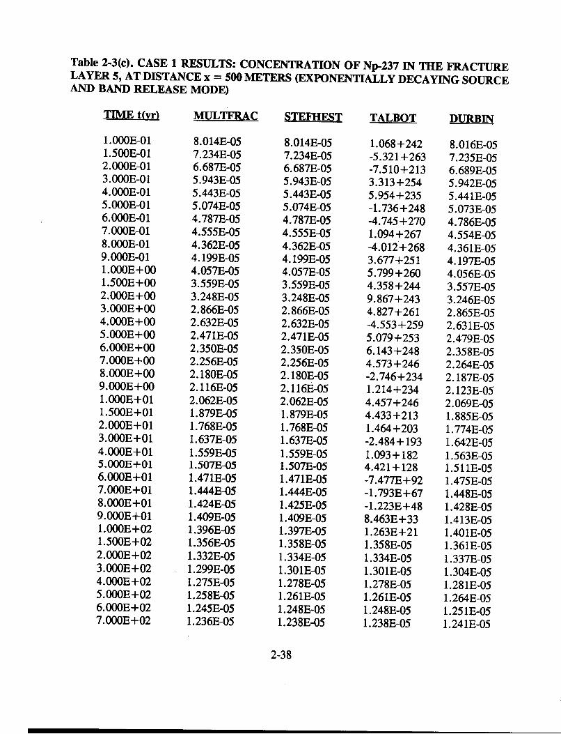
Table 2-3(c). CASE 1 RESULTS: CONCENTRATION OF Np-237 IN THE FRACTURELAYER 5, AT DISTANCE x = 500 METERS (EXPONENTIALLY DECAYING SOURCEAND BAND RELEASE MODE)
TIME t(yr) MULTFRAC STEFHEST TALBOT DURBIN
1.OOOE-011.500E-012.OOOE-013.OOOE-014.000E-015.OOOE-016.000E-017.000E-018.000E-019.000E-011.000E+OO1.500E+OO2.000E+OO3.000E+OO4.000E+OO5.000E+OO6.000E+OO7.000E+OO8.000E+OO9.000E+OO1.OOOE+011.500E+012.000E+013.000E+014.000E+015.OOOE+016.OOOE+017.000E+018.000E+019.000E+011.OOOE+021.500E+022.OOOE+023.OOOE+024.000E+025.000E+026.OOOE+027.000E+02
8.014E-057.234E-056.687E-055.943E-055.443E-055.074E-054.787E-054.555E-054.362E-054.199E-054.057E-053.559E-053.248E-052.866E-052.632E-052.471E-052.350E-052.256E-052.180E-052.116E-052.062E-051. 879E-051.768E-051.637E-051.559E-051.507E-051.471E-051.444E-051.424E-051.409E-051.396E-051.356E-051.332E-051.299E-051.275E-051.258E-051.245E-051.236E-05
8.014E-057.234E-056.687W-055.943E-055.443E-055.074E-054.787W-054.555E-054.362E-054.199E-054.057W-053.559E-053.248E-052.866E-052.632E-052.471E-052.350E-052.256E-052.180E-052.116E-052.062E-051.879E-051.768E-051.637E-051.559E-051.507E-051.471E-051.444E-051.425E-051.409E-051.397E-051.358E-051.334E-051.301E-051.278E-051.261E-051.248E-051.238E-05
1.068+242-5.321 +263-7.510+2133.313+2545.954+235-1.736+248-4.745+2701.094+267-4.012+2683.677+2515.799+2604.358+2449.867+2434.827+261-4.553+2595.079+2536.143+2484.573 +246-2.746+2341.214+2344.457+2464.433+2131.464+203-2.484+ 1931.093+1824.421 + 128-7.477E+92-1.793E+67-1.223E+488.463E+331.263E+211.358E-051.334E-051.301E-051.278E-051.261E-051.248E-051.238E-05
8.016E-057.235E-056.689E-055.942E-055.441E-055.073E-054.786E-054.554E-054.361E-054.197E-054. 056E-o53.557E-053.246E-052.865E-052.631E-052.479E-052.358E-052.264E-052.187E-052.123E-052.069E-051. 885E-051.774E-051.642E-051.563E-051.51 1E-051.475E-051.448E-051.428E-051.413E-051.401E-051.361E-051.337E-051.304E-051.281E-051.264E-051.2511E-051.241E-05
2-38

Table 2-3(c). CASE 1 RESULTS: CONCENTRATION OF Np-237 IN THE FRACTURELAYER 5, AT DISTANCE x = 500 METERS (EXPONENTIALLY DECAYING SOURCEAND BAND RELEASE MODE) (Continued)
TIME t(yr) MULTFRAC STEFHEST TALBOT DURBIN
8.OOOE+029.OOOE+021.OOOE+031.500E+032.OOOE+033.OOOE+034.000E+035.000E+036.000E+037.000E+038.000E+039.000E+031.OOOE+041.500E+042.000E+043.000E+044.000E+045.OOOE+046.OOOE+047.OOOE+048.000E+049.OOOE+041.OOOE+051.500E+052.OOOE+053.000E+054.000E+055.000E+056.000E+057.OOOE+058.000E+059.000E+051.000E+06
1.233E-051.263E-051.409E-051.619E-041. 192E-038.880E-032.425E-024.458E-026.73 1E-028.959E-021.051E-011. 123E-011.135E-019.175E-026.929E-024.287E-022.946E-022.174E-021.685E-021.354E-021.11 8E-029.420E-038.075E-034.420E-032.857E-031.525E-039.664E-046.733E-044.982E-043.843E-043.057E-042.489E-042.064E-04
1.236E-051.266E-051.411E-051.619E-041. 193E-038.880E-032.425E-024.458E-026.731E-028.959E-021.05lE-011.123E-011. 135E-019.175E-026.929E-024.287E-022.946E-022.174E-021.685E-021.354E-021.11 8E-029.420E-038.075E-034.420E-032.858E-031.525E-039.665E-046.733E-044.982E-043.844E-043.057E-042.489E-042.065E-04
1.236E-051.266E-051.411E-051.619E-041. 193E-038.880E-032.425E-024.458E-026.731E-028.959E-021.051E-011. 123E-011. 135E-019.175E-026.929E-024.287E-022.946E-022.174E-021.685E-021.354E-021.11 8E-029.420E-038:075E-034.420E-032.858E-031.525E-039.665E-046.733E-044.982E-043.844E-043.057E-042.489E-042.065E-04
1.238E-051.263E-051.413E-051.619E-041. 189E-038.881E-032.425E-024.458E-026.731E-028.959E-021.051E-011. 123E-011. 135E-019.175E-026.929E-024.287E-022.946E-022.174E-021.685E-021.354E-02
-1.118E-029.420E-038.075E-034.420E-032.858E-031.525E-039.665E-046.733E-044.982E-043.844E-043.057E-042.489E-042.065E-04
2-39

-M M M M M M M - - - M M M M M - - -
103
102
101
2 10°
*E0
-b 102
C
D
.'
E 103
t'j
0L
1o-6
10-7lo-, 10° 101 102 10 3 104 10 5 1loB
Time, t(yr)
Figure 2-2(c). Cumulative mass of Np-237 per unit in the fracture vs. time at different positions x = 100, 200, and500 meters (Exponentially decaying source and band release mode).

Table 2-4(a). CASE 1 RESULTS: CUMULATIVE MASS OF Np-237 IN THE FRACTUREAT DISTANCE x = 100 METERS (EXPONENTIALLY DECAYING SOURCE ANDBAND RELEASE MODE)
TIME (yr)
1.OOOE-011.500E-012.OOOE-013.OOOE-014.OOOE-015.OOOE-016.OOOE-017.OOOE-018.OOOE-019.OOOE-011.000E+OO1 .500E+OO2.000E+O03.OOOE+OO4.OOOE+OO5.000E+OO6.000E+OO7.000E+OO8.OOOE+009.OOOE+OO1.OOOE+011.500E+012.000E+013.OOOE+014.OOOE+015.OOOE+016.000E+017.OOOE+018.000E+019.OOOE+011.OOOE+021.500E+022.OOOE+023.OOOE+024.OOOE+025.OOOE+026.OOOE+02
MULTFRAC
1.543E-062.204E-062.825E-063.980E-065.051E-066.059E-067.016E-067.932E-068.813E-069.664E-061.049E-051.430E-051.775E-052.395E-052.954E-053.472E-053.960E-054.425E-054.871E-055.301E-055.718E-057.660E-059.439E-051.271E-041.594E-043.594E-041. 863E-037.060E-031.874E-023.939E-027.087E-024.223E-011.107E+OO3.326E+OO6.417E+O01.015E+011.438E+01
STEFEHEST
1.543E-062.204E-062.825E-063.980E-065.051E-066.059E-067.016E-067.932E-068.813E-069.664E-061.049E-051.430E-051.775E-052.395E-052.954E-053.472E-053.960E-054.425E-054.870E-055.301E-055.718E-057.659E-059.438E-051.270E-041.594E-043.594E-041. 863E-037.060E-031.874E-023.939E-027.087E-024.223E-011.107E+OO3.326E+OO6.417E+0O1.015E+011.438E+01
2-41

Table 2-4(a). CASE 1 RESULTS: CUMULATIVE MASS OF Np-237 IN THE FRACTUREAT DISTANCE x = 100 METERS (EXPONENTIALLY DECAYING SOURCE ANDBAND RELEASE MODE) (Continued)
TIME (vr)
7.000E+028.000E+029.000E+021.OOOE+031.500E+032.000E+033.000E+034.000E+035.000E+036.000E+037.000E+038.000E+039.000E+031.OOOE+041.500E+042.000E+043.000E+044.000E+045.000E+046.000E+047.000E+048.000E+049.000E+041.OOOE+051.500E+052.000E+053.000E+054.OOOE+055.000E+056.000E+057.000E+058.OOOE+059.000E+051.OOOE+06
MULTFRAC
1.901E+012.397E+012.919E+013.465E+016.454E+019.740E+011.684E+022.438E+023.220E+023.676E+023.867E+023.988E+024.075E+024.142E+024.338E+024.440E+024.551E+024.614E+024.656E+024.686E+024.709E+024.728E+024.743E+024.755E+024.798E+024.822E+024.851E+024.867E+024.878E+024.886E+024.891E+024.896E+024.900E+024.903E+02
STEFHEST
1.901E+012.397E+012.919E+013.465E+016.454E+019.740E+011.684E+022.438E+023.220E+023.676E+023.867E+023.988E+024.075E+024.141E+024.338E+024.440E+024.551E+024.613E+024.655E+024.685E+024.709E+024.727E+024.743E+024.755E+024.798E+024.823E+024.852E+024.868E+024.879E+024.887E+024.893E+024.897E+024.901E+024.904E+02
2-42
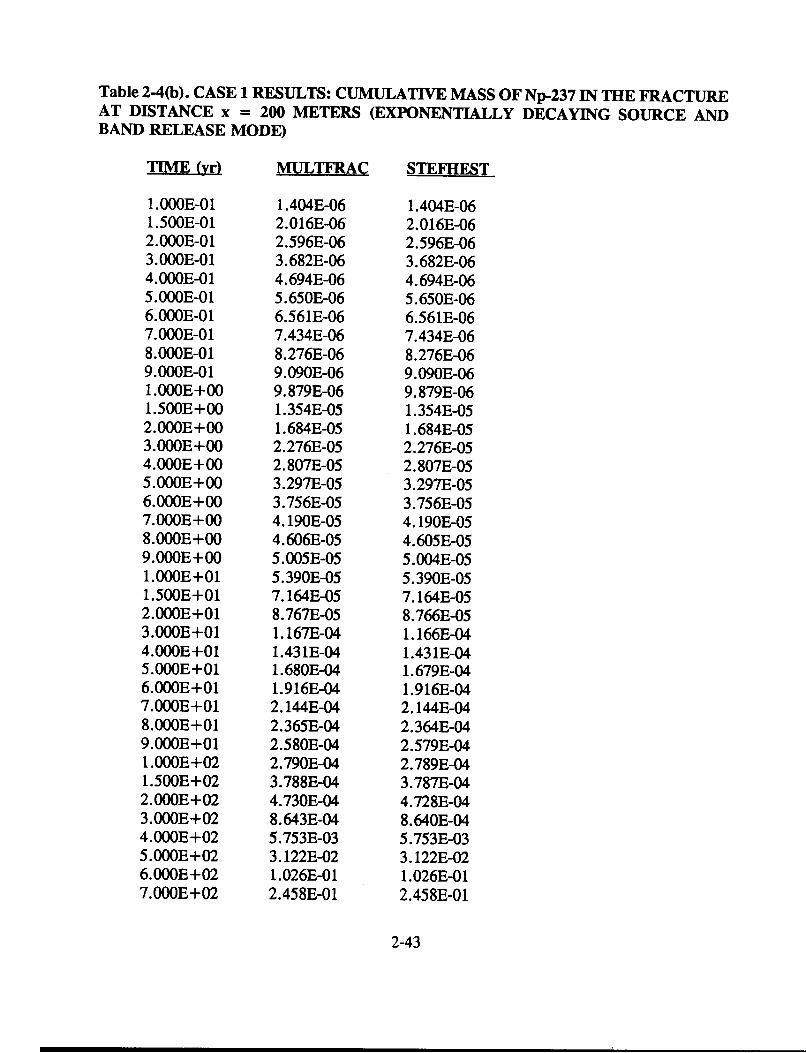
Table 2-4(b). CASE 1 RESULTS: CUMULATIVE MASS OF Np-237 IN THE FRACTUREAT DISTANCE x = 200 METERS (EXPONENTIALLY DECAYING SOURCE ANDBAND RELEASE MODE)
MULTFRAC STEFIEST
1.OOOE-011.500E-012.OOOE-013.OOOE-014.OOOE-015.OOOE-016.OOOE-017.OOOE-018.OOOE-019.OOOE-011.OOOE+OO1.500E+OO2.OOOE+OO3.OOOE+004.OOOE+O05.OOOE+OO6.OOOE+007.OOOE+OO8.OOOE+OO9.OOOE+001.OOOE+011.500E+012.OOOE+013.OOOE+014.OOOE+015.OOOE+016.OOOE+017.OOOE+018.000E+019.OOOE+011.OOOE+021.500E+022.OOOE+023.OOOE+024.OOOE+025.OOOE+026.OOOE+027.OOOE+02
1.404E-062.016E-062.596E-063.682E-064.694E-065.650E-066.561E-067.434E-068.276E-069.090E-069.879E-061.354E-051.684E-052.276E-052.807E-053.297E-053.756E-054.190E-054.606E-055.005E-055.390E-057.164E-058.767E-051. 167E-041.431E-041.680E-041.916E-042.144E-042.365E-042.580E-042.790E-043.788E-044.730E-048.643E-045.753E-033.122E-021.026E-012.458E-01
1.404E-062.016E-062.596E-063.682E-064.694E-065.650E-066.561E-067.434E-068.276E-069.090E-069.879E-061.354E-051.684E-052.276E-052.807E-053.297E-053.756E-054.190E-054.605E-055.004E-055.390E-057.164E-058.766E-051. 166E-041.431E-041.679E-041.916E-042.144E-042.364E-042.579E-042.789E-043.787E-044.728E-048.640E-045.753E-033.122E-021.026E-012.458E-01
2-43
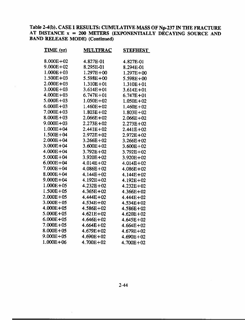
Table 2-4(b). CASE 1 RESULTS: CUMULATIVE MASS OF Np-237 IN THE FRACTUREAT DISTANCE x = 200 METERS (EXPONENTIALLY DECAYING SOURCE ANDBAND RELEASE MODE) (Continued)
TIME (yrl
8.OOOE+029.OOOE+021.000E+031.500E+032.OOOE+033.000E+034.OOOE+035.000E+036.000E+037.OOOE+038.OOOE+039.OOOE+031.OOOE+041.500E+042.OOOE+043.000E+044.000E+045.000E+046.OOOE+047.OOOE+048.000E+049.000E+041.000E+051.500E+052.OOOE+053.000E+054.000E+055.000E+056.OOOE+057.000E+058.OOOE+059.000E+051.000E+06
MULTFRAC
4.827E-018.295E-011.297E+005.598E+001.310E+013.614E+016.747E+011.050E+021.460E+021. 803E+022.066E+022.273E+022.441E+022.972E+023.266E+023.600E+023.792E+023.920E+024.014E+024.086E+024.144E+024.192E+024.232E+024.365E+024.444E+024.534E+024.586E+024.621E+024.646E+024.664E+024.679E+024.690E+024.700E+02
STEFHEST
4.827E-018.294E-011.297E+005.598E+001.310E+013.614E+016.747E+011.050E+021.460E+021.803E+022.066E+022.273E+022.441E+022.972E+023.266E+023.600E+023.792E+023.920E+024.014E+024.086E+024.144E+024.192E+024.232E+024.366E+024.444E+024.534E+024.586E+024.620E+024.645E+024.664E+024.679E1+024.690E+024.700E+02
2-44

Table 2-4(c). CASE 1 RESULTS: CUMULATIVE MASS OF Np-237 IN THE FRACTUREAT DISTANCE x = 500 METERS (EXPONENTIALLY DECAYING SOURCE ANDBAND RELEASE MODE)
TIME (yr)
1.OOOE-011.500E-012.OOOE-013.OOOE-014.OOOE-015.OOOE-016.OOOE-017.OOOE-018.OOOE-019.OOOE-011.OOOE+OO1.500E+OO2.OOOE+OO3.OOOE+OO4.OOOE+OO5.OOOE+OO6.OOOE+OO7.OOOE+OO8.OOOE+OO9.OOOE+OO1.OOOE+011.500E+012.OOOE+013.OOOE+014.OOOE+015.OOOE+016.OOOE+017.OOOE+018.OOOE+019.OOOE+011.OOOE+021.500E+022.OOOE+023.OOOE+024.OOOE+025.OOOE+026.OOOE+027.OOOE+02
MULTFRAC
9.712E-071.351E-061.698E-062.327E-062.895E-063.420E-063.913E-064.379E-064.825E-065.253E-065.666E-067.558E-069.254E-061.229E-051.503E-051.758E-051.999E-052.229E-052.451E-052.665E-052.874E-053.855E-054.765E-056.461E-058.056E-059.588E-051.108E-041.253E-041.397E-041.538E-041.679E-042.366E-043.039E-044.355E-045.644E-046.913E-048.167E-049.410E-04
STEFHEST
9.712E-071.351E-061.698E-062.327E-062.895E-063.420E-063.913E-064.379E-064.825E-065.253E-065.665E-067.558E-069.254E-061.229E-051.503E-051.758E-051.999E-052.229E-052.450E-052.665E-052.874E-053.854E-054.763E-056.459E-058.053E-059.583E-051.107E-041.252E-041.396E-041.537E-041.677E-042.364E-043.036E-044.351E-045.638E-046.906E-048.158E-049.400E-04
2-45

Table 2-4(c). CASE 1 RESULTS: CUMULATIVE MASS OF Np-237 IN THE FRACTUREAT DISTANCE x = 500 METERS (EXPONENTIALLY DECAYING SOURCE ANDBAND RELEASE MODE) (Continued)
MULTFRAC STEFHEST
8.000E+029.000E+021.OOOE+031.500E+032.000E+033.000E+034.000E+035.000E+036.000E+037.000E+038.000E+039.000E+031.OOOE+041.500E+042.000E+043.000E+044.000E+045.000E+046.000E+047.000E+048.000E+049.000E+041 .OOOE+051 .500E+052.000E+053.000E+054.000E+055.000E+056.000E+057.000E+058.000E+059.000E+051.OOOE+06
1.065E-031. 189E-031.321E-034.087E-033.215E-024.659E-012.068E+005.480E+001.106E+011.894E+012.875E+013.968E+015. 101E+011.031E+021.430E+021.975E+022.330E+022.583E+022.774E+022.925E+023.048E+023.150E+023.238E+023.535E+023.713E+023.921E+024.042E+024.122E+024.180E+024.224E+024.258E+024.286E+024.309E+02
1.063E-031. 188E-031.320E-034.086E-033.215E-024.659E-012.068E+005.480E+001.106E+011.894E+012.875E+013.968E+015.101E+011.031E+021.430E+021.975E+022.330E+022.583E+022.774E+022.925E+023.048E+023.150E+023.238E+023.535E+023.713E+023.920E+024.042E+024.123E+024.181E+024.224E+024.259E+024.286E+024.309E+02
2-46

m m m - -m m m m m m - -
101
10°
C
Cr
C:
a.C,a,8D)
DM._
Dr
10-
1 2
10-3
10-4
4.4
10-5
10-6 L1-2 10- 100 101
I Distance, z(m)102
Figure 2-2(d). Relative concentration of Np-237 in rock vs. distance z at time T = 5,000 years and distances fromthe source x = 100, 200 and 500 meters (Exponentially decaying source and step release mode).
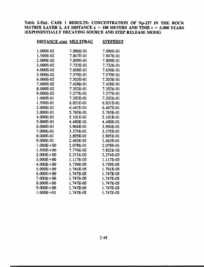
Table 2-5(a). CASE 1 RESULTS: CONCENTRATION OF Np-237 IN THE ROCKMATRIX LAYER 2, AT DISTANCE x = 100 METERS AND TIME t = 5,000 YEARS(EXPONENTIALLY DECAYING SOURCE AND STEP RELEASE MODE)
DISTANCE z(m) MULTFRAC STEFHEST
1.OOOE-021.500E-022.OOOE-023.OOOE-024.OOOE-025.OOOE-026.OOOE-027.OOOE-028.OOOE-029.OOOE-021.OOOE-011.500E-012.OOOE-013.OOOE-014.OOOE-015.OOOE-016.OOOE-017.OOOE-018.OOOE-019.OOOE-011.OOOE+O01.500E+OO2.OOOE+OO3.OOOE+OO4.OOOE+OO5.OOOE+OO6.OOOE+OO7.OOOE+OO8.OOOE+OO9.OOOE+O01.OOOE+01
7.886E-017.847E-017.809E-017.732E-017.656E-017.579E-017.503E-017.428E-017.352E-017.277E-017.202E-016.831E-016.467E-015.765E-015. 101E-014.480E-013.904E-013.375E-012.895E-012.463E-012.078E-017.774E-022.371E-021.117E-033.739E-051.761E-051.747E-051.747E-051.747E-051.747E-051.747E-05
7.886E-O17.847E-O17.809E-O17.732E-017.656E-017.579E-017.503E-017.428E-017.352E-017.277E-017.202E-016.831E-016.467E-015.765E-015. 101E-014.480E-013.904E-013.375E-012.895E-012.463E-012.078E-017.832E-022.374E-021. 117E-033.739E-051.761E-051.747E-051.747E-051.747E-051.747E-051.747E-05
2-48

Table 2-5(b). CASE 1 RESULTS: CONCENTRATION OF Np-237 IN THE ROCKMATRIX LAYER 3, AT DISTANCE x = 200 METERS AND TIME t = 5,000 YEARS(EXPONENTIALLY DECAYING SOURCE AND STEP RELEASE MODE)
DISTANCE z(m) MULTFRAC STEFHEST
1.OOOE-021.500E-022.OOOE-023.OOOE-024.OOOE-025.OOOE-026.OOOE-027.OOOE-028.OOOE-029.OOOE-021.OOOE-011.500E-012.OOOE-013.OOOE-014.OOOE-015.OOOE-016.OOOE-017.OOOE-018.OOOE-019.OOOE-011.OOOE+OO1.500E+OO2.OOOE+OO3.OOOE+OO4.OOOE+OO5.OOOE+OO6.OOOE+OO7.OOOE+OO8.OOOE+OO9.OOOE+OO1.OOOE+01
3.973E-013.947E-013.922E-013.871E-013.821E-013.771E-013.722E-013.673E-013.624E-013.576E-013.528E-013.295E-013.072E-012.657E-012.283E-011.947E-011.649E-011.387E-011.158E-019.604E-027.904E-022.671E-027.473E-033.370E-041. 884E-051.254E-051.248E-051.248E-051.248E-051.248E-051.248E-05
3.973E-013.947E-013.922E-013.871E-013.821E-013.771E-013.722E-013.673E-013.624E-013.576E-013.528E-013.295E-013.072E-012.657E-012.283E-011.947E-011.649E-011.387E-011.158E-019.604E-027.904E-022.671E-027.473E-033.370E-041. 884E-051.254E-051.248E-051.248E-051.248E-051.248E-051.248E-05
2-49

Table 2-5(c). CASE 1 RESULTS: CONCENTRATION OF Np-237 IN THE ROCKMATRIX LAYER 5, AT DISTANCE x = 500 METERS AND TIME t = 5,000 YEARS(EXPONENTIALLY DECAYING SOURCE AND STEP RELEASE MODE)
DISTANCE z(m) MULTFRAC STEFIEST
1.OOOE-021.500E-022.OOOE-023.OOOE-024.OOOE-025.OOOE-026.OOOE-027.OOOE-028.OOOE-029.OOOE-021.OOOE-011.500E-012.OOOE-013.OOOE-014.OOOE-015.OOOE-016.OOOE-017.OOOE-018.OOOE-019.OOOE-011.OOOE+001.500E+002.OOOE+003.OOOE+004.OOOE+005.OOOE+00
4.293E-024.199E-024.107E-023.927E-023.754E-023.588E-023.428E-023.274E-023.126E-022.983E-022.847E-022.242E-021.752E-021.045E-026.045E-033.390E-031.844E-039.744E-045.01 1E-042.523E-041.259E-041.223E-051.625E-061.048E-051.048E-051.048E-05
4.294E-024.200E-024.107E-023.927E-023.754E-023.588E-023.428E-023.274E-023.126E-022.983E-022.847E-022.241E-021.751E-021.045E-026.040E-033.384E-031.837E-039.660E-044.921E-042.429E-041.161E-041.823E-061.505E-087.758E-133.047E-15-9.383E-17
2-50
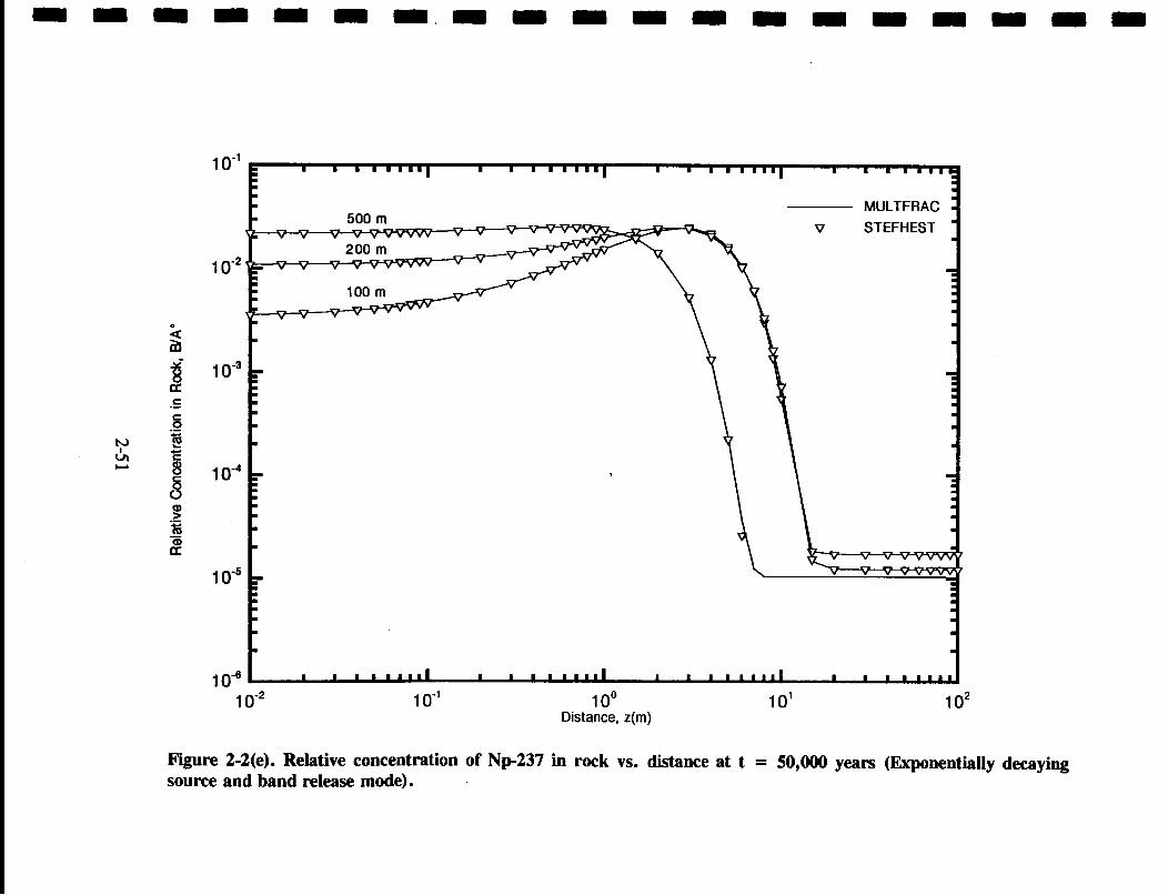
m- m m m m m - m m - mm m mm
lo-,
10-2
t!J
C.A%C
8ID
0)
10-3
10-4
1 0-5
1-6
1 -2 lo-, 100 10'Distance, z(m)
102
Figure 2-2(e). Relative concentration of Np-237 in rock vs. distance at t = 50,000 years (Exponentially decayingsource and band release mode).

Table 2-6(a). CASE 1 RESULTS: CONCENTRATION OF Np-237 IN THE ROCKMATRIX LAYER 2, AT DISTANCE X = 100 METERS AND TIME t = 50,000 YEARS(EXPONENTIALLY DECAYING SOURCE AND BAND RELEASE MODE)
DISTANCE z(m) MULTFRAC STEFHEST
1.OOOE-021.500E-022.OOOE-023.OOOE-024.OOOE-025.OOOE-026.OOOE-027.OOOE-028.OOOE-029.OOOE-021.OOOE-011.500E-012.OOOE-013.OOOE-014.OOOE-015.OOOE-016.OOOE-017.OOOE-018.OOOE-019.OOOE-011.OOOE+OO1.500E+OO2.OOOE+OO3.OOOE+OO4.OOOE+OO5.OOOE+OO6.OOOE+OO7.OOOE+OO8.OOOE+OO9.OOOE+OO1.OOOE+011.500E+012.OOOE+013.OOOE+014.OOOE+015.OOOE+016.OOOE+017.OOOE+01
3.566E-033.633E-033.699E-033.832E-033.965E-034.098E-034.230E-034.363E-034.495E-034.627E-034.759E-035.416E-036.070E-037.361E-038.630E-039.872E-031. 108E-021.226E-021.340E-021.450E-021.555E-022.008E-022.321E-022.505E-022.203E-021.649E-021.070E-026. 101E-033.077E-031.383E-035.603E-041.825E-051.724E-051.719E-051.724E-051.724E-051.724E-051.724E-05
3.566E-033.633E-033.699E-033.832E-033.965E-034.098E-034.230E-034.363E-034.495E-034.627E-034.759E-035.417E-036.070E-037.362E-038.630E-039.872E-031. 108E-021.226E-021.340E-021.450E-021.555E-022.008E-022.321E-022.505E-022.203E-021.649E-021.070E-026. 101E-033.077E-031.383E-035.603E-041.825E-051.724E-051.724E-051.724E-051.724E-051.724E-051.724E-05
2-52

Table 2-6(a). CASE 1 RESULTS: CONCENTRATION OF Np-237 IN THE ROCKMATRIX LAYER 2, AT DISTANCE X = 100 METERS AND TIME t = 50,000 YEARS(EXPONENTIALLY DECAYING SOURCE AND BAND RELEASE MODE) (Continued)
DISTANCE z(m) MULTFRAC STEFHEST
8.OOOE+019.OOOE+011.OOOE+02
1.724E-051.724E-051.724E-05
1.724E-051.724E-051.724E-05
Table 2-6(b). CASE 1 RESULTS: CONCENTRATION OF Np-237 IN THE ROCKMATRIX LAYER 3, AT DISTANCE x = 200 METERS AND TIME t = 50,000 years(EXPONENTIALLY DECAYING SOURCE AND BAND RELEASE MODE)
DISTANCE z(m) MULTFRAC STEFHEST
1.OOOE-021.500E-022.000E-023.OOOE-024.OOOE-025.OOOE-026.OOOE-027.OOOE-028.OOOE-029.OOOE-021.000E-011.500E-012.OOOE-013.OOOE-014.OOOE-015.OOOE-016.000E-017.000E-018.OOOE-019.OOOE-011.000E+001.500E+002.000E+003.000E+004.OOOE+005.OOOE+006.OOOE+00
1.090E-021.095E-021. 101E-021.112E-021. 123E-021. 134E-021. 144E-021. 155E-021. 166E-021.177E-021.187E-021.241E-021.293E-021.395E-021.494E-021.589E-021.680E-021.767E-021.849E-021.927E-022.001E-022.296E-022.466E-022.455E-022.092E-021.566E-021.043E-02
1.090E-021.095E-021. 101E-021.112E-021. 123E-021. 134E-021. 144E-021. 155E-021. 166E-021. 177E-021. 187E-021.241E-021.293E-021.395E-021.494E-021.589E-021.680E-021.767E-021. 849E-021.927E-022.001E-022.296E-022.466E-022.455E-022.092E-021.566E-021.043E-02
2-53

Table 2-6(b). CASE 1 RESULTS: CONCENTRATION OF Np-237 IN THE ROCKMATRIX LAYER 3, AT DISTANCE x = 200 METERS AND TIME t = 50,000 years(EXPONENTIALLY DECAYING SOURCE AND BAND RELEASE MODE) (Continued)
DISTANCE z(m) MULTFRAC STEFHEST
7.OOOE+008.OOOE+009.OOOE+001.OOOE+011.500E+012.OOOE+013.OOOE+014.OOOE+015.OOOE+016.OOOE+017.000E+018.OOOE+019.OOOE+011.OOOE+02
6.232E-033.361E-031.644E-037.339E-041.468E-051.231E-051.231E-051.23 1E-051.23 1E-051.23 1E-051.23 1E-051.231E-051.231E-051.23 1E-05
6.232E-033.361E-031.644E-037.339E-041.532E-051.23 1E-051.231E-051.231E-051.231E-051.231E-051.231E-051.231E-051.231E-051.231E-05
Table 2-6(c). CASEMATRIX LAYER 3,
1 RESULTS: CONCENTRATION OF Np-237 IN THE ROCKAT DISTANCE x = 500 METERS AND TIME t = 50,000 YEARS
(EXPONENTIALLY DECAYING SOURCE AND BAND RELEASE MODE)
DISTANCE z(m) MULTFRAC STEFHEST
1.OOOE-021.500E-022.OOOE-023.OOOE-024.OOOE-025.OOOE-026.OOOE-027.OOOE-028.OOOE-029.OOOE-021.OOOE-011.500E-012.OOOE-013.OOOE-014.OOOE-015.OOOE-016.OOOE-01
2.184E-022.189E-022.195E-022.206E-022.217E-022.228E-022.239E-022.249E-022.260E-022.270E-022.279E-022.326E-022.367E-022.434E-022.481E-022.509E-022.519E-02
2.184E-022.189E-022.195E-022.206E-022.217E-022.228E-022.239E-022.249E-022.259E-022.270E-022.279E-022.326E-022.367E-022.434E-022.481E-022.509E-022.518E-02
2-54

Table 2-6(c). CASE 1 RESULTS: CONCENTRATION OF Np-237 IN THE ROCKMATRIX LAYER 3, AT DISTANCE x = 500 METERS AND TIME t = 50,000 YEARS(EXPONENTIALLY DECAYING SOURCE AND BAND RELEASE MODE) (Continued)
DISTANCE z(m) MULTFRAC STEFHEST
7.OOOE-018.OOOE-019.OOOE-O11.OOOE+OO1.500E+OO2.OOOE+OO3.OOOE+OO4.OOOE+OO5.OOOE+OO6.OOOE+OO7.OOOE+OO8.OOOE+OO9.OOOE+OO1.OOOE+011.500E+O12.OOOE+013.OOOE+O14.OOOE+O15.OOOE+O16.OOOE+O17.OOOE+O18.OOOE+O19.OOOE+O11.OOOE+02
2.510E-022.485E-022.445E-022.390E-021.966E-021.425E-025.357E-031.341E-032.350E-043.646E-051.245E-051.046E-051.035E-051.034E-051.034E-051.034E-051.034E-051.034E-051.034E-051.034E-051.034E-051.034E-051.034E-051.034E-05
2.510E-022.485E-022.444E-022.390E-021.965E-021.424E-025.347E-031.331E-032.247E-042.613E-052.1 OE-061. 192E-074.741E-091.336E-106.509E-162.326E-17-6.476E-22-3.892E-265.217E-30-2.151E-33-3. 111E-36-3.367E-39-3.562E-42-3.746E-45
2.3.2 Case 2 Results
This test case examines, as before, the spatial and temporal variationof the concentration of Cm-245, as well as its cumulative mass flux in the fracture. In addition,the spatial variations of the concentration in the rock matrix are also investigated. The sourceterms correspond now to a periodically fluctuating one with exponential decay, and the assignedresidual concentrations are almost one order of magnitude less than their counterparts in the caseof Np-237. The input data pertaining to this test case is presented in Table 2-7. Note that theimplementation of a periodically decaying source restricts the use of benchmarking algorithmsother than Talbot's and Durbin's for reasons presented earlier.
2-55

Figure 2-3(a) shows the spatial relative concentration profiles of Cm-245 observed in the fracture layers for simulation times corresponding to 103, 5x10³ and 5 X10⁴
years. A comparison of our results with the ones obtained from the two numerical inversionalgorithms. Tables 2-8(a) through 2-8(c) show that these are in excellent agreement.
Figure 2-3(b) shows the temporal relative concentration of Np-237observed in the fracture at three different observation points: 100, 200 and 500 metersdownstream from the source, located in the second, third and fifth layer respectively, for a bandrelease mode. The observations here are similar to the ones reported for Np-237 except that inthe present case the upper tail of the concentration profiles is akin to the assigned initialconcentrations of the various fracture layers of interest. A comparison of our results with thoseyielded by Talbot's and Durbin's algorithms lying within the acceptable range of concentrations(see Tables 2-9(a) through 2-9(c)) seem to indicate good agreement. Note that Talbot'salgorithm performance is further reduced in this case, where correct predictions of theconcentrations at the three monitoring points seem to be registered only for times greater than40, 80 and 300 years respectively.
Figure 2-3(c) depicts the time-dependent evolution of the cumulativemass release (per unit width of the fracture) profile at three different observation points in thefracture as in the previous example. Because of its robustness, Durbin's algorithm is selectedas the benchmark. A comparison of our analytical solution results with those yielded byDurbin's solution (see Tables 2-10(a) through 2-10(c)) indicate excellent agreement. Note thatall three profiles will tend to become asymptotic to three specific values of the cumulative massnamely: 2.175 x10², 1.237 x10², and 40.9 (UA/m)3.
Figures 2-3(d) and 2-3(e) show the concentration profiles in the rockmatrix at three position downstream from the source (i.e., x = 100m, 200m, and 500m) fora step release and band release respectively. Comparison of our analytical results against thoseyielded by the two approximate solution methods (see Tables 2-1l(a) through 2-12(c)) indicateexcellent agreement.
The assumption of zero dispersive flux in the fracture raises thequestion of the range of validity of the analytical solutions presented in this report. This matterdepends very much on the importance of the hydrodynamic dispersion effects prevailing in thefracture. This matter has been investigated and quantified numerically by Ahn et al., (1985)(i.e., for the case of zero initial concentrations in both fracture and rock) who suggested thathydrodynamic dispersion D (see Bear, 1972) should meet the following criterion
3 UA: Arbitrary Units of Activity/meter.
2-56

10u' bi
i ( ( DP ilt! )1,
in order to validate the use of the zero fracture dispersion solution. The maximum permissiblevalue of Di for any layer i would correspond to a minimum of 254.0 m2/yr for Test Case 1, and245.0 m 2/yr for Test Case 2. Expressed in terms of dispersivity (i.e., Di/u) these wouldcorrespond approximately to a value of 16 m in both cases.
Table 2-7. NPUT PARAMETERS FOR CASE 2SOURCE WITH EXPONENTIAL DECAY
PERIODICALLY FLUCTUATING
SPECIES Cm-245
T 1/2 8.5 x 10³ yr
Release Mode:StepBand Leaching Time
AO
Q
NA5 x 103 yr
1.0
0. 1 (M3/yr)
0.75
0.25
5.0 yr
LA YER L' m b-M) u;mly J__________1 50.0 5.OE-03 10.0 0.01
2 75.0 4.OE-03 12.5 0.008
3 100.0 3.OE-03 16.666 0.006
4 150.0 2.OE-03 25.0 0.004
5 0o l.5E-03 33.333 0.002
2-57
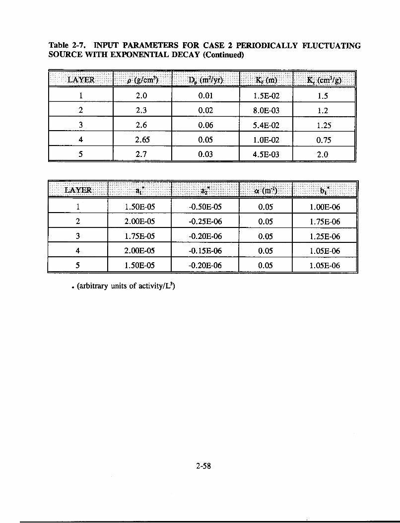
Table 2-7. INPUT PARAMETERS FOR CASE 2 PERIODICALLYSOURCE WITH EXPONENTIAL DECAY (Continued)
FLUCTUATING
1 2.0 0.01 1.5E-02 1.5
2 2.3 0.02 8.OE-03 1.2
3 2.6 0.06 5.4E-02 1.25
4 2.65 0.05 1.OE-02 0.75
5 2.7 0.03 4.5E-03 2.0
LAYER J- I I a| - ) I b1 i
1 1.50E-05 -0.50E-05 0.05 1.OOE-06
2 2.OOE-05 -0.25E-06 0.05 1.75E-06
3 1.75E-05 -0.20E-06 0.05 1.25E-06
4 2.OOE-05 -0. 15E-06 0.05 1.05E-06
5 1.50E-05 -0.20E-06 0.05 1.05E-06
. (arbitrary units of activity/L 3)
2-58

I~mm No- m - m O - m -m
100
10-2
(UccLLC
C 10-._c
iO5C 1 0-5
a)
a:1 0-510-7
10- 100 101 . 102 - 10 3104
Distance, x(m)
Figure 2-3(s). Relative concentration of Cm-245 vs. distance in the fracture at different times t = 1,000, 5,000, and50,000 years (Periodically fluctuating source with exponential decay).

Table 2-8(a). CASE 2 RESULTS: CONCENTRATION OF Cm-245 IN THE FRACTUREAT TIME t = 1,000 YEARS (PERIODICALLY FLUCTUATIING SOURCE WITHEXPONENTIAL DECAY AND STEP RELEASE MODE)
DISTANCE x(m) MULTFRAC TALBOT DURBIN
1.OOOE-011.500E-012.OOOE-013.OOOE-014.OOOE-015.OOOE-016.OOOE-017.OOOE-018.OOOE-019.OOOE-011.OOOE+OO1.500E+OO2.OOOE+OO3.OOOE+OO4.OOOE+OO5.OOOE+OO6.OOOE+OO7.OOOE+OO8.000E+OO9.OOOE+OO1.OOOE+011.500E+012.000E+013.000E+014.OOOE+015.OOOE+016.OOOE+017.OOOE+018.000E+019.OOOE+011.OOOE+021.500E+022.OOOE+023.OOOE+024.OOOE+025.OOOE+026.OOOE+027.OOOE+02
6.908E-016.906E-016.904E-016.900E-016.896E-016.891E-016.887E-016.883E-016.879E-016.874E-016.870E-016.849E-016.827E-016.785E-016.742E-016.700E-016.657E-016.614E-016.572E-016.529E-016.486E-016.273E-016.061E-015.639E-015.223E-014.815E-014.338E-013.881E-013.448E-013.040E-012.661E-018.846E-021. 177E-022.178E-043.934E-061. 145E-061.066E-061.047E-06
6.908E-016.906E-016.904E-016.900E-016.896E-016.891E-016.887E-016.883E-016.879E-016.874E-016.870E-016.849E-016.827E-016.785E-016.742E-016.700E-016.657E-016.614E-016.572E-016.529E-016.486E-016.273E-016.061E-015.639E-015.223E-014.815E-014.338E-013.881E-013.447E-013.040E-012.661E-018.842E-021. 176E-022.174E-043.925E-061. 145E-061.066E-061.047E-06
6.908E-016.906E-016.904E-016.900E-016.896E-016.891E-016.887E-016.883E-016.879E-016.874E-016.870E-016.849E-016.827E-016.785E-016.742E-016.700E-016.657E-016.614E-016.572E-016.529E-016.486E-016.273E-016.061E-015.639E-015.223E-014.815E-014.338E-013.881E-013.447E-013.040E-012.661E-018.842E-021. 176E-022.172E-043.953E-061. 154E-061.080E-061.061E-06
2-60
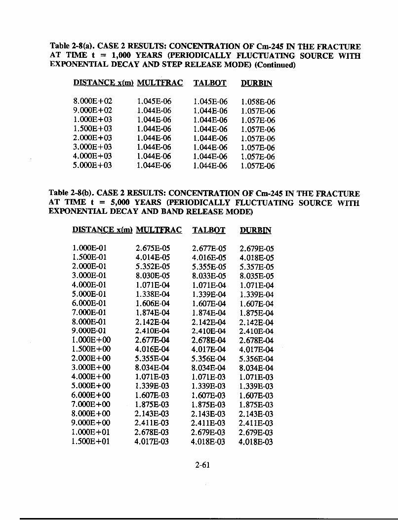
Table 2-8(a). CASE 2 RESULTS: CONCENTRATION OF Cm-245 IN THE FRACTUREAT TIME t = 1,000 YEARS (PERIODICALLY FLUCTUATING SOURCE WITHEXPONENTIAL DECAY AND STEP RELEASE MODE) (Continued)
DISTANCE x(m) MULTFRAC TALBOT DURBIN
8.000E+029.000E+021.OOOE+031.500E+032.000E+033.000E+034.000E+035.000E+03
1.045E-061.044E-061.044E-061.044E-061.044E-061.044E-061.044E-061.044E-06
1.045E-061.044E-061.044E-061.044E-061.044E-061.044E-061.044E-061.044E-06
1.058E-061.057E-061.057E-061.057E-061.057E-061.057E-061.057E-061.057E-06
Table 2-8(b). CASE 2 RESULTS: CONCENTRATION OF Cm-245 IN THE FRACTUREAT TIME t = 5,000 YEARS (PERIODICALLY FLUCTUATING SOURCE WITHEXPONENTIAL DECAY AND BAND RELEASE MODE)
DISTANCE x(m) MULTFRAC TALBOT DURBIN
1.OOOE-011.500E-012.OOOE-013.000E-014.000E-015.000E-016.000E-017.000E-018.000E-019.OOOE-011.000E+001.500E+002.000E+003.000E+004.000E+005.000E+006.OOOE+007.000E+008.000E+009.000E+001.OOOE+011.500E+01
2.675E-054.014E-055.352E-058.030E-051.071E-041.338E-041.606E-041.874E-042.142E-042.410E-042.677E-044.016E-045.355E-048.034E-041.071E-031.339E-031.607E-031.875E-032.143E-032.41 lE-032.678E-034.017E-03
2.677E-054.016E-055.355E-058.033E-051.071E-041.339E-041.607E-041.874E-042.142E-042.410E-042.678E-044.017E-045.356E-048.034E-041.071E-031.339E-031.607E-031.875E-032.143E-032.41 IE-032.679E-034.018E-03
2.679E-054.018E-055.357E-058.035E-051.071E-041.339E-041.607E-041.875E-042.142E-042.410E-042.678E-044.017E-045.356E-048.034E-041.071E-031.339E-031.607E-031.875E-032.143E-032.41 1E-032.679E-034.018E-03
2-61

Table 2-8(b). CASE 2 RESULTS: CONCENTRATION OF Cm-245 IN THE FRACTUREAT TIME t = 5,000 YEARS (PERIODICALLY FLUCTUATING SOURCE WITHEXPONENTIAL DECAY AND BAND RELEASE MODE) (Continued)
DISTANCE x(m) MULTFRAC TALBOT DURBIN
2.OOOE+013.OOOE+014.OOOE+015.OOOE+016.OOOE+017.OOOE+018.OOOE+019.OOOE+011.OOOE+021.500E+022.OOOE+023.OOOE+024.OOOE+025.OOOE+026.OOOE+027.000E+028.OOOE+029.000E+021.OOOE+031.500E+032.OOOE+033.OOOE+034.OOOE+035.OOOE+03
5.355E-038.021E-031.067E-021.330E-021.644E-021.952E-022.253E-022.545E-022.828E-024.409E-025.491E-025.303E-024.201E-022.974E-021. 893E-021.097E-025.839E-032.877E-031.319E-031.019E-054.896E-074.762E-074.762E-074.762E-07
5.355E-038.022E-031.067E-021.330E-021.644E-021.952E-022.253E-022.545E-022.828E-024.409E-025.491E-025.303E-024.201E-022.974E-021.893E-021.097E-025.838E-032.876E-031.3188E-031.0188E-054.896E-074.762E-074.762E-074.762E-07
5.355E-038.022E-031.067E-021.330E-021.644E-021.952E-022.253E-022.545E-022.828E-024.409E-025.491E-025.303E-024.201E-022.974E-021. 893E-021.097E-025.838E-032.877E-031.318E-031.019E-054.969E-074.840E-074.840E-074.840E-07
Table 2-8(c). CASE 2 RESULTS: CONCENTRATION OF Cm-245 IN THE FRACTUREAT TIME t = 50,000 YEARS (PERIODICALLY FLUCTUATING SOURCE WITHEXPONENTIAL DECAY AND BAND RELEASE MODE)
DISTANCE x(m) MULTFRAC TALBOT DURBIN
1.000E-011.500E-012.OOOE-013.000E-014.000E-01
5.953E-088.949E-081. 194E-071.794E-072.393E-07
5.991E-088.987E-081. 198E-071.797E-072.397E-07
5.991E-088.987E-081. 198E-071.797E-072.397E-07
2-62

Table 2-8(c). CASE 2 RESULTS: CONCENTRATION OF Cm-245 IN THE FRACTUREAT TIME t = 50,000 YEARS (PERIODICALLY FLUCTUATING SOURCE WITHEXPONENTIAL DECAY AND BAND RELEASE MODE) (Continued)
DISTANCE x(m) MULTFRAC TALBOT DURBIN
5.OOOE-016.OOOE-017.OOOE-018.OOOE-019.OOOE-011.OOOE+001.500E+002.OOOE+003.OOOE+004.OOOE+005.OOOE+006.OOOE+007.OOOE+008.OOOE+009.OOOE+001.OOOE+011.500E+012.OOOE+013.OOOE+014.OOOE+015.OOOE+016.OOOE+017.OOOE+018.OOOE+019.OOOE+011.OOOE+021.500E+022.OOOE+023.OOOE+024.OOOE+025.OOOE+026.OOOE+027.OOOE+028.OOOE+029.OOOE+021.OOOE+031.500E+032.OOOE+03
2.992E-073.591E-074.190E-074.789E-075.389E-075.988E-078.983E-071.198E-061.797E-062.396E-062.995E-063.595E-064.194E-064.793E-065.392E-065.991E-068.987E-061. 198E-051.797E-052.395E-052.993E-053.717E-054.439E-055.158E-055.875E-056.589E-051.11 8E-041.651E-042.286E-042.701E-042.984E-043.167E-043.250E-043.240E-043.149E-042.988E-041.695E-046.162E-05
2.996E-073.595E-074.194E-074.793E-075.392E-075.991E-078.987E-071. 198E-061.797E-062.397E-062.996E-063.595E-064.194E-064.793E-065.393E-065.992E-068.987E-061. 198E-051.797E-052.395E-052.993E-053.717E-054.439E-055.158E-055.875E-056.589E-051.11 8E-041.651E-042.286E-042.701E-042.984E-043.167E-043.250E-043.240E-043.149E-042.988E-041.695E-046.162E-05
2.996E-073.595E-074.194E-074.793E-075.392E-075.991E-078.987E-071. 198E-061.797E-062.397E-062.996E-063.595E-064.194E-064.793E-065.393E-065.992E-068.987E-061. 198E-051.797E-052.395E-052.993E-053.717E-054.439E-055.158E-055.876E-056.590E-051.11 8E-041.650E-042.286E-042.701E-042.984E-043.167E-043.250E-043.240E-043.149E-042.990E-041.696E-046.162E-05
2-63
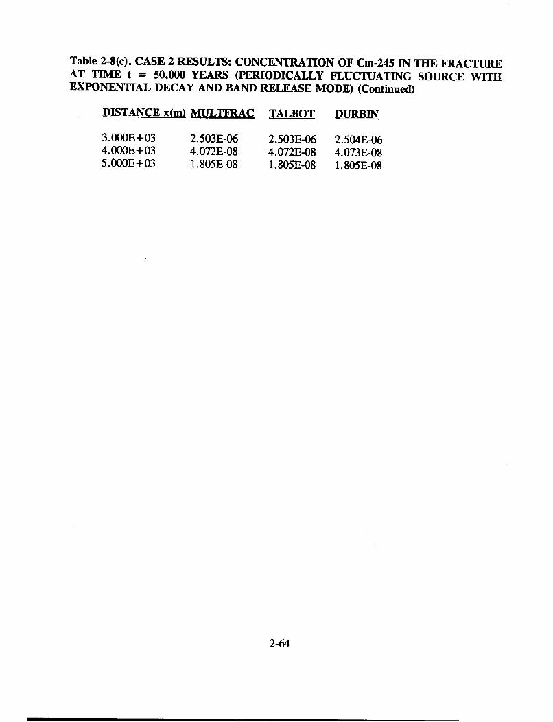
Table 2-8(c). CASE 2 RESULTS: CONCENTRATION OF Cm-245 IN THE FRACTUREAT TIME t = 50,000 YEARS (PERIODICALLY FLUCTUATING SOURCE WITHEXPONENTIAL DECAY AND BAND RELEASE MODE) (Continued)
DISTANCE x(m) MULTFRAC TALBOT DURBIN
3.OOOE+034.OOOE+035.OOOE+03
2.503E-064.072E-081.805E-08
2.503E-064.072E-081. 805E-08
2.504E-064.073E-081.805E-08
2-64
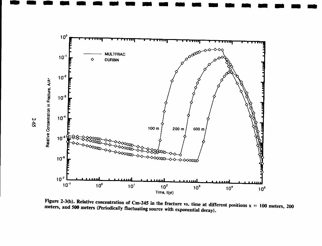
m mM 'm mm-- -- - - - - M mm
1 0O
10'1
C
U.LLa;
S
FS
8
4>CreS0
S:
10-2
10-3
1 o-4
0-5
t.J
10-3
1o-7 L10-' 100 10o 102 103 104 105
Time, t(yr)
Figure 2-3(b). Relative concentration of Cm-245 in the fracture vs. time at different positions x = 100 meters, 200meters, and 500 meters (Periodically fluctuating source with exponential decay).

Table 2-9(a). CASE 2 RESULTS: CONCENTRATION OF Cm-245 IN THE FRACTUREIN LAYER 2, AT DISTANCE x = 100 METERS (PERIODICALLY FLUCTUATINGSOURCE WITH EXPONENTIAL DECAY AND STEP RELEASE MODE)
TIME (v) MULTFRAC TALBOT DURBIN
1 .OOOE-011.500E-012.000E-013.OOOE-014.000E-015.000E-016.000E-017.000E-018.000E-019.000E-011.OOOE+001.500E+002.000E+003.000E+004.000E+005.000E+006.000E+007.000E+008.000E+009.000E+001.000E+011 .500E+012.OOOE+013.000E+014.000E+015.000E+016.OOOE+017.000E+018.000E+019.000E+011.OOOE+021.500E+022.000E+023.000E+024.000E+025.000E+026.000E+027.000E+02
1.250E-051. 151E-051.079E-059.765E-069.052E-068.51 1E-068.082E-067.728E-067.43 1E-067.175E-066.95 1E-066.147E-065.632E-064.986E-064.583E-064.301E-064.090E-063.923E-063.788E-063.675E-063.578E-063.248E-063.049E-062.810E-062.667E-062.570E-062.703E-061.027E-056.893E-052.757E-047.497E-049.519E-032.718E-027.209E-021. 152E-011.522E-011.834E-012.095E-01
2.184+188-4.441 +246-4.572+2612.005+2434.431 +259-5.666+2602.925+2224.361+238-2.506+2722.301+238-1.678+213-1.604+242-1.656+2422.438+224-2.694+1601.553+2008.813+1591.114+1312.442+109-2.759E+926.475+1725.749E+87-1.702E+45-5.177E+022.680E-062.568E-062.708E-061.050E-057.056E-052.814E-047.634E-049.442E-032.723E-027.214E-021. 152E-011.522E-011.833E-012.094E-01
1.253E-051. 154E-051.081E-059.791E-069.076E-068.535E-068.105E-067.75 1E-067.453E-067.196E-066.973E-066.167E-065.650E-065.002E-064.598E-064.316E-064.103E-063.936E-063.800E-063.686E-063.590E-063.259E-063.058E-062.837E-062.673E-062.544E-062.669E-061.054E-057.0533E-052.813E-047.635E-049.442E-032.723E-027.215E-021.152E-011.522E-011.833E-012.094E-01
2-66

Table 2-9(a). CASE 2 RESULTS: CONCENTRATION OF Cm-245 IN THE FRACTUREIN LAYER 2, AT DISTANCE x = 100 METERS (PERIODICALLY FLUCTUATINGSOURCE W1TH EXPONENTIAL DECAY AND STEP RELEASE MODE) (Continued)
TIME (y) MULTFRAC TALBOT DURBIN
8.OOOE+029.OOOE+021.OOOE+031.500E+032.OOOE+033.OOOE+034.OOOE+035.OOOE+036.OOOE+037.OOOE+038.OOOE+039.OOOE+031.000E+041.500E+042.OOOE+043.OOOE+044.OOOE+045.OOOE+046.OOOE+047.OOOE+048.OOOE+049.OOOE+041.OOOE+051.500E+052.OOOE+053.OOOE+054.OOOE+055.OOOE+056.OOOE+057.OOOE+058.OOOE+059.OOOE+051.OOOE+06
2.315E-012.502E-012.661E-013.189E-013.456E-013.640E-013.615E-013.499E-011.570E-018.635E-025.556E-023.869E-022.828E-028.507E-033.400E-037.630E-042.121E-046.589E-052.190E-057.622E-062.742E-061.012E-063.806E-073.471E-093.800E- 115.910E-151.100E-182.258E-224.932E-261. 124E-292.642E-336.361E-371.560E-40
2.314E-012.501E-012.661E-013.189E-013.455E-013.640E-013.615E-013.499E-011.570E-018.636E-025.556E-023.869E-022.828E-028.508E-033.400E-037.630E-042.121E-046.589E-052.190E-057.622E-062.742E-061.012E-063.806E-073.471E-093.800E- 115.982E-154.007E-165.580E-166.163E-163.204E-162.729E-162.835E-177.371E-17
2.314E-012.501E-012.661E-013.189E-013.455E-013.640E-013.615E-013.499E-011.570E-018.636E-025.556E-023.869E-022.828E-028.508E-033.400E-037.629E-042.121E-046.590E-052.190E-057.622E-062.742E-061.012E-063.806E-073.471E-093.800E- 115.896E-151.408E-17-7.545E-181.497E-175.328E-182.488E-17-5.385E-18-8.938E-19
2-67

Table 2-9(b). CASE 2 RESULTS: CONCENTRATION OF Cm-245 IN THE FRACTUREIN LAYER 3, AT DISTANCE x = 200 METERS (PERIODICALLY FLUCTUATINGSOURCE WITH EXPONENTIAL DECAY AND BAND RELEASE MODE)
TIME (y) MULTFRAC TALBOT DURBIN
1.OOOE-011.500E-012.OOOE-0l3.000E-014.OOOE-O15.OOOE-016.OOOE-017.OOOE-0l8.OOOE-O19.OOOE-011.OOOE+001.500E+002.OOOE+003.OOOE+004.OOOE+005.OOOE+006.000E+0O7.OOOE+008.OOOE+009.000E+001.OOOE+011.500E+O12.OOOE+O13.OOOE+014.OOOE+015.OOOE+O16.OOOE+017.OOOE+018.000E+O19.OOOE+011.OOOE+021.500E+022.OOOE+023.OOOE+024.OOOE+025.OOOE+026.OOOE+027.000E+02
1.453E-051.399E-051.355E-051.288E-051.235E-051. 193E-051. 156E-051. 124E-051.096E-051.071E-051.048E-059.584E-068.938E-068.032E-067.405E-066.933E-066.560E-066.255E-065.998E-065.778E-065.586E-064.900E-064.464E-063.919E-063.581E-063.344E-063.167E-063.027E-062.913E-062.818E-062.737E-062.457E-062.284E-062.133E-061.718E-051.944E-048.550E-042.285E-03
5.273+2341.474+113-3.527E+691.812+2094.523+2561.438+236-4.659+264-2.491 +267-1.440+249-4.417+247-2.991+2691.216+2681.989+2619.815+2701.001+263-2.075 +225-8.843+254-1.437+214-1.726+228-3.403+236-3.213+209-3.235+211-5.380+189-6.937+186-7.301+1622.565+113-2.135E+80-2.093E+579.066E+391.164E+26-2.442E+ 152.460E-062.284E-062.135E-061.740E-051.966E-048.640E-042.305E-03
1.456E-051.401E-051.358E-051.290E-051.238E-051. 195E-051. 159E-051. 127E-051.099E-051.073E-051.05lE-059.608E-068.961E-068.054E-067.426E-066.954E-066.580E-066.274E-066.017E-065.796E-065.604E-064.917E-064.479E-063.933E-063.593E-063.356E-063.178E-063.037E-062.923E-062.827E-062.746E-062.482E-062.312E-062.127E-061.756E-051.963E-048.643E-042.305E-03
2-68

Table 2-9(b). CASE 2 RESULTS: CONCENTRATION OF Cm-245 IN THE FRACTUREIN LAYER 3, AT DISTANCE x = 200 METERS (PERIODICALLY FLUCTUATINGSOURCE WITH EXPONENTIAL DECAY AND BAND RELEASE MODE) (Continued)
TIME (y) MULTFRAC TALBOT DURBIN
8.OOOE+029.OOOE+021.000E+031.500E+032.OOOE+033.OOOE+034.000E+035.OOOE+036.OOOE+037.OOOE+038.OOOE+039.000E+031.OOOE+041.500E+042.OOOE+043.000E+044.OOOE+045.OOOE+046.OOOE+047.000E+048.000E+049.OOOE+041.OOOE+051.500E+052.000E+053.OOOE+054.OOOE+055.000E+056.000E+057.000E+058.000E+059.OOOE+051.000E+06
4.644E-037.835E-031. 177E-023.776E-026.558E-021.103E-011.389E-011.555E-011.562E-011.235E-019.306E-027.086E-025.491E-021. 882E-027.907E-031. 853E-035.256E-041.651E-045.529E-051.934E-056.985E-062.585E-069.747E-078.950E-099.832E-111.534E-142.861E-185.879E-221.285E-252.929E-296.889E-331.659E-364.071E-40
4.636E-037.826E-031. 176E-023.775E-026.557E-021. 103E-011.388E-011.555E-011.562E-011.235E-019.307E-027.087E-025.491E-021.882E-027.907E-031. 853E-035.256E-041.651E-045.529E-051.934E-056.985E-062.585E-069.747E-078.951E-099.832E-1 11.540E-147.985E-171.400E-162.871E-163.949E-161. 189E-162.184E-162.190E-17
4.636E-037.826E-031. 176E-023.775E-026.557E-021. 103E-011.388E-011.555E-011.562E-011.235E-019.307E-027.087E-025.491E-021. 882E-027.907E-031.853E-035.256E-041.650E-045.529E-051.934E-056.985E-062.585E-069.747E-078.951E-099.832E-1 1-5.189E-07-7.419E-08-4.753E-07-3.961E-07-6.632E-082.972E-072.641E-072.377E-07
2-69

Table 2-9(c). CASE 2 RESULTS: CONCENTRATION OF Cm-245 IN THE FRACTUREIN LAYER 5, AT DISTANCE x = 500 METERS (PERIODICALLY FLUCTUATINGSOURCE WITH EXPONENTIAL DECAY AND BAND RELEASE MODE)
TIME (v) MULTFRAC TALBOT DURBIN
1.000E-011.500E-012.000E-013.000E-014.000E-015.000E-016.000E-017.000E-018.000E-019.000E-011.OOOE+001 .500E+002.000E+003.000E+004.000E+005.000E+006.000E+007.000E+008.000E+009.000E+001.OOOE+011.500E+012.000E+013.000E+014.000E+015.000E+016.000E+017.000E+018.000E+019.OOOE+011.000E+021.500E+022.OOOE+023.OOOE+024.000E+025.OOOE+026.OOOE+027.OOOE+02
7.219E-066.453E-065.929E-065.232E-064.774E-064.442E-064.187E-063.982E-063.813E-063.671E-063.549E-063.121E-062.858E-062.539E-062.344E-062.211E-062.111E-062.033E-061.971E-061.918E-061.874E-061.723E-061.633E-061.525E-061.460E-061.415E-061.382E-061.356E-061.335E-061.317E-061.302E-061.255E-061.231E-061.207E-061. 191E-061. 177E-061.164E-061. 152E-06
8.689+218-4.152+271-2.893+ 1904.875+2507.382+2271.802+2613.548+242-1.281 +2422.024+261-1.002+273-2.800+2353.914+264-8.926+2484.032+250-9.699+245-2.552+260-4.125+265-1.167+2452.827+2651.118+2323.661 +256-3.137+2413.227+198-1.671 +205-1.511+142-1.568+172-3.968+ 1811.606+ 143-1.064+116-4.803E+93-3.967E+75-4.242E+22-2.924E-051.207E-061. 192E-061. 178E-061. 165E-061. 154E-06
7.238E-066.471E-065.946E-065.249E-064.790E-064.457E-064.201E-063.996E-063.826E-063.684E-063.561E-063.132E-062.868E-062.565E-062.369E-062.233E-062.133E-062.054E-061.991E-061.938E-061. 893E-061.741E-061.649E-061.540E-061.475E-061.430E-061.396E-061.370E-061.349E-061.331E-061.316E-061.269E-061.245E-061.220E-061.205E-061. 192E-061.181E-061. 174E-06
2-70

Table 2-9(c). CASE 2 RESULTS: CONCENTRATION OF Cm-245 IN THE FRACTUREIN LAYER 5, AT DISTANCE x = 500 METERS (PERIODICALLY FLUCTUATINGSOURCE WITH EXPONENTIAL DECAY AND BAND RELEASE MODE) (Continued)
TIME (v) MULTFRAC TALBOT DURBIN
8.OOOE+029.OOOE+02l.OOOE+031.500E+032.OOOE+033.OOOE+034.OOOE+035.OOOE+036.OOOE+037.OOOE+038.OOOE+039.OOOE+031.OOOE+041.500E+042.OOOE+043.OOOE+044.OOOE+045.OOOE+046.OOOE+047.OOOE+048.OOOE+049.OOOE+041.OOOE+051.500E+052.OOOE+053.OOOE+054.OOOE+055.OOOE+056.OOOE+057.OOOE+058.OOOE+059.OOOE+051.OOOE+06
1. 144E-061. 136E-061. 145E-061.OO1E-051.396E-041.784E-035.934E-031. 178E-021.817E-022.417E-022.844E-023.013E-022.974E-021.860E-029.942E-032.878E-038.989E-042.984E-041.036E-043.716E-051.367E-055.133E-061.958E-061.860E-082.077E-103.296E-146.195E-181.279E-212.805E-256.410E-291.510E-323.642E-368.945E-40
1. 144E-061. 137E-061. 145E-069.994E-061.394E-041.783E-035.932E-031.178E-021.816E-022.417E-022.844E-023.013E-022.974E-021.860E-029.942E-032.878E-038.989E042.984E-041.036E-043.716E-051.367E-055.133E-061.958E-061.860E-082.077E-103.322E-146.849E-171.129E-167.443E-175.215E-17-2.602E-17-1.457E-17-2.802E-17
1.164E-061. 145E-061. 154E-061.008E-051.392E-041.783E-035.932E-031. 178E-021.816E-022.417E-022.844E-023.013E-022.974E-021.860E-029.942E-032.878E-038.989E-042.984E-041.035E-043.71 1E-051.367E-055.133E-061.956E-061.860E-082.077E-101.447E-075.450E-07-4.404E-07-3.660E-07-5.327E-074.667E-07-8.083E-087.299E-08
2-71

m mm - -mm - -
103
102
M 100a
: 10-'
U.
§ 1o-0- 1 o-3
0CLIa 0-
-!j
1o-
1 0-7 '
lo-1 100 11o 102 10 3 i04 10 5 106Time, t(yr)
Figure 2-3(c). Cumulative mass of Cm-245 per unit in the fracture vs. time at different positions x = 100, 200, and500 meters (Periodically fluctuating source with exponential decay).

Table 2-10(a). CASE 2 RESULTS: CUMULATIVE MASS OF Cm-245 IN THEFRACTURE AT DISTANCE x = 100 METERS (PERIODICALLY FLUCTUATINGSOURCE WITH EXPONENTIAL DECAY AND BAND RELEASE MODE)
MULTFRAC DURBIN
1.OOOE-O11.500E-O12.OOOE-013.OOOE-O14.OOOE-O15.OOOE-O16.OOOE-017.OOOE-018.OOOE-019.OOOE-O11.OOOE+O01.500E+OO2.OOOE+003.OOOE+004.OOOE+005.OOOE+OO6.OOOE+007.OOOE+008.OOOE+009.OOOE+001.OOOE+011.500E+012.OOOE+013.OOOE+014.OOOE+O15.OOOE+016.OOOE+O17.OOOE+018.OOOE+O19.OOOE+011.OOOE+021.500E+022.OOOE+023.OOOE+024.OOOE+025.OOOE+026.OOOE+027.OOOE+02
1.448E-072.047E-072.603E-073.627E-074.566E-075.443E-076.272E-077.062E-077.820E-078.550E-079.256E-071.251E-061.545E-062.073E-062.550E-062.993E-063.413E-063.813E-064.198E-064.571E-064.934E-066.632E-068.203E-061.112E-051.385E-051.647E-051.904E-052.456E-056.008E-052.289E-047.479E-042.207E-021. 119E-016.078E-011.551E+OO2.895E+004.579E+006.548E+OO
1.451E-072.05 1E-072.609E-073.636E-074.577E-075.457E-076.288E-077.080E-077.840E-078.572E-079.280E-071.255E-061.549E-062.079E-062.558E-063.003E-063.423E-063.825E-064.211E-064.585E-064.949E-066.652E-068.229E-061.117E-051.392E-051.653E-051.910E-052.402E-055.680E-052.151E-047.101E-042.164E-021. 106E-016.043E-O11.546E+002.888E+004.570E+0O6.537E+OO
2-73

Table 2-10(a). CASE 2 RESULTS: CUMULATIVE MASS OF Cm-245 IN THEFRACTURE AT DISTANCE x = 100 METERS (PERIODICALLY FLUCTUATINGDECAYING SOURCE AND BAND RELEASE MODE) (Continued)
TIME (yr)
8.OOOE+029.OOOE+021.OOOE+031.500E+032.OOOE+033.OOOE+034.OOOE+035.OOOE+036.OOOE+037.OOOE+038.OOOE+039.000E+031.OOOE+041.500E+042.OOOE+043.OOOE+044.OOOE+045.OOOE+046.OOOE+047.OOOE+048.OOOE+049.OOOE+041.OOOE+051.500E+052.OOOE+053.OOOE+054.OOOE+055.OOOE+056.OOOE+057.OOOE+058.OOOE+059.OOOE+051.OOOE+06
MULTERAC
8.756E+001.117E+011.375E+012.853E+014.522E+018.096E+011. 173E+021.530E+021.780E+021.896E+021.965E+022.012E+022.045E+022.124E+022.152E+022.169E+022.173E+022.174E+022.175E+022.175E+022.175E+022.175E+022.175E+022.175E+022.175E+022.175E+022.175E+022.175E+022.175E+022.175E+022.175E+022.175E+022.175E+02
DURBIN
8.744E+001.115E+011.374E+012.852E+014.520E+018.094E+011.173E+021.529E+021.780E+021.896E+021.965E+022.012E+022.045E+022.124E+022.152E+022.169E+022.174E+022.175E+022.175E+022.174E+022.174E+022.173E+022.173E+022.172E+022.172E+022.174E+022.179E+022.184E+02NANANANANA
2-74

Table 2-10(b). CASE 2 RESULTS: CUMULATIVE MASS OF Cm-245 IN THEFRACTURE AT DISTANCE x = 200 METERS (PERIODICALLY FLUCTUATINGSOURCE WITH EXPONENTIAL DECAY AND BAND RELEASE MODE)
IME (yr)
1.OOOE-Ol1.500E-O12.OOOE-0l3.OOOE-014.OOOE-0l5.OOOE-O16.OOOE-017.OOOE-018.OOOE-019.OOOE-011.OOOE+001.500E+002.OOOE+OO3.000E+004.OOOE+005.000E+006.OOOE+007.000E+008.000E+009.OOOE+001.OOOE+011.500E+O12.000E+013.OOOE+014.OOOE+015.OOOE+016.OOOE+017.000E+018.000E+019.OOOE+O11.OOOE+021.500E+022.OOOE+023.OOOE+024.OOOE+025.OOOE+026.OOOE+027.OOOE+02
MULTFRAC
1.544E-072.257E-072.945E-074.264E-075.525E-076.738E-077.912E-079.052E-071.016E-061. 125E-061.230E-061.73 1E-062.193E-063.038E-063.809E-064.524E-065.198E-065.839E-066.451E-067.040E-067.608E-061.021E-051.255E-051.671E-052.045E-052.391E-052.716E-053.026E-053.322E-053.609E-053.886E-055.178E-056.360E-058.532E-051.439E-049.618E-045.744E-032.093E-02
DURBIN
NANANANANANANANANANANANANANANANANANANANA7.628E-061.024E-051.259E-051.677E-052.052E-052.399E-052.725E-053.035E-053.333E-053.620E-053.899E-055.202E-056.397E-058.581E-051.435E-049.541E-045.708E-032.084E-02
2-75

Table 2-10(b). CASE 2 RESULTS: CUMULATIVE MASS OF Cm-245 IN THEFRACTURE AT DISTANCE x = 200 METERS (PERIODICALLY FLUCTUATINGSOURCE WITH EXPONENTIAL DECAY AND BAND RELEASE MODE) (Continued)
MULTFRAC DURBIN
8.000E+029.000E+021.OOOE+031.500E+032.000E+033.000E+034.000E+035.OOOE+036.000E+037.000E+038.000E+039.000E+031.OOOE+041.500E+042.000E+043.000E+044.000E+045.OOOE+046.000E+047.000E+048.000E+049.000E+041.OOOE+051.500E+052.000E+053.000E+054.000E+055.OOOE+056.000E+057.000E+058.000E+059.000E+051.OOOE+06
5.497E-021. 167E-012.142E-011.424E+004.016E+001.295E+012.553E+014.033E+015.622E+017.028E+018.104E+018.917E+019.542E+O11.119E+021.181E+021.222E+021.232E+021.235E+021.236E+021.237E+021.237E+021.237E+021.237E+021.237E+021.237E+021.237E+021.237E+021.237E+021.237E+021.237E+021.237E+021.237E+021.237E+02
5.480E-021. 164E-012.138E-011.423E+004.014E+001.295E+012.552E+014.032E+015.621E+017.028E+018.103E+018.917E+019.542E+01NANANANA -NANANANANANANANANANANANANANANANA
2-76

TABLE 2-10(c). CASE 2 RESULTS: CUMULATIVE MASS OF Cm-245 IN THEFRACTURE AT DISTANCE x = 500 METERS (PERIODICALLY FLUCTUATINGSOURCE WITH EXPONENTIAL DECAY AND BAND RELEASE MODE)
MULTFRAC DURBIN
1 .OOOE-O11.500E-O12.OOOE-O13.OOOE-O14.OOOE-O15.OOOE-O16.OOOE-O17.OOOE-O18.OOOE-O19.OOOE-O11.OOOE+OO1 .500E+O02.OOOE+OO3.OOOE+OO4.OOOE+OO5.OOOE+OO6.OOOE+OO7.OOOE+O08.OOOE+OO9.OOOE+OO1.OOOE+O11 .500E+O12.OOOE+O13.OOOE+O14.OOOE+O15.OOOE+O16.OOOE+O17.OOOE+O18.OOOE+O19.OOOE+O11.OOOE+021.500E+022.OOOE+023.OOOE+024.OOOE+025.OOOE+026.OOOE+027.OOOE+02
8.996E-081.240E-071.549E-072.104E-072.603E-073.063E-073.494E-073.902E-074.292E-074.666E-075.027E-076.684E-078.174E-071.086E-061.329E-061.557E-061.772E-061.980E-062.180E-062.374E-062.564E-063.459E-064.297E-065.870E-067.360E-068.796E-061.019E-051. 156E-051.291E-051.423E-051.554E-052.192E-052.813E-054.032E-055.231E-056.415E-057.587E-058.746E-05
NANANANANANANANANANANANANANANANANANANANA2.582E-063.486E-064.331E-065.920E-067.423E-068.873E-061.028E-051.167E-051.302E-051.436E-051.568E-052.212E-052.839E-054.069E-055.280E-056.477E-057.662E-058.838E-05
2-77

TABLE 2-10(c). CASE 2 RESULTS: CUMULATIVE MASS OF Cm-245 IN THEFRACTURE AT DISTANCE x = 500 METERS (PERIODICALLY FLUCTUATINGSOURCE WITH EXPONENTIAL DECAY AND BAND RELEASE MODE) (Continued)
TIME (yr) MULTFRAC
8.OOOE+029.000E+021.OOOE+031.500E+032.OOOE+033.OOOE+034.OOOE+035.OOOE+036.OOOE+037.OOOE+038.OOOE+039.OOOE+031.OOOE+041.500E+042.OOOE+043.OOOE+044.OOOE+045.OOOE+046.OOOE+047.OOOE+048.OOOE+049.OOOE+041.OOOE+051 .500E+052.OOOE+053.OOOE+054.OOOE+055.OOOE+056.OOOE+057.OOOE+058.OOOE+059.OOOE+051.OOOE+06
9.896E-051.104E-041.217E-042.765E-043.020E-037.903E-024.459E-011.323E+002.820E+OO4.945E+OO7.596E+o01 .055E+O11.355E+012.580E+O13.273E+O13.840E+014.009E+014.063E+014.082E+014.088E+014.090E+014.091E+014.092E+014.092E+014.092E+O14.092E+014.092E+014.092E+014.092E+014.092E+O14.092E+O14.092E+O14.092E+O1
1 .OO1E-041.11 6E-041.230E-042.782E-043.014E-037.893E-024.455E-O11.322E+002.819E+004.943E+007.595E+001.054E+011.355E+01NANANANANANANANANANANANANANANANANANANANA
2-78

m m M M - m m m m m m M M M M M M M M
100
10-
C
I9ra
10-2
10-3
10-4
10-5
o-
10-6
10-210- 100 101 102
Distance, z(m)
Figure 2-3(d). Relative concentration of Cm-245 in rock vs. distance z at time t = 5,000 years and distances fromthe source x = 100, 200, and 500 meters (Periodically fluctuating source with exponential decay).

Table 2-11(a). CASE 2 Results: CONCENTRATION OF Cm-245 IN THE ROCK MATRIXLAYER 2, AT DISTANCE x = 100 METERS AND TIME t = 5,000 YEARS(PERIODICALLY FLUCTUATING SOURCE WITH EXPONENTIAL DECAY AND STEPRELEASE MODE)
DISTANCE z(m) MULTFRAC TALBOT DURBIN
1.500E-022.OOOE-023.OOOE-024.OOOE-025.OOOE-026.OOOE-027.OOOE-028.OOOE-029.OOOE-021.OOOE-011.500E-012.OOOE-013.OOOE-014.OOOE-015.OOOE-016.OOOE-017.OOOE-018.OOOE-019.OOOE-011.000E+001.500E+002.OOOE+003.OOOE+004.OOOE+005.OOOE+006.OOOE+007.OOOE+008.OOOE+009.OOOE+001.OOOE+011.500E+012.OOOE+013.OOOE+014.OOOE+015.OOOE+016.OOOE+017.OOOE+01
3.446E-013.421E-013.373E-013.326E-013.278E-013.231E-013.184E-013.137E-013.091E-013.045E-012.819E-012.602E-012.194E-011.826E-011.499E-011.214E-019.689E-027.624E-025.913E-024.518E-029.377E-031.319E-038.914E-061.076E-061.164E-061.164E-061. 164E-061. 164E-061. 164E-061.164E-061.164E-061. 164E-061. 164E-061. 164E-061.164E-061. 164E-061.164E-06
3.446E-013.421E-013.373E-013.326E-013.278E-013.231E-013.184E-013.137E-013.091E-013.045E-012.819E-012.601E-012.194E-011.826E-011.499E-011.214E-019.689E-027.624E-025.912E-024.517E-029.376E-031.318E-038.910E-061. 173E-061.164E-061. 164E-061. 164E-061.164E-061. 164E-061.164E-061. 164E-061. 164E-061. 164E-061. 164E-061.164E-061.164E-061.164E-06
3.446E-013.421E-013.373E-013.326E-013.278E-013.231E-013.184E-013.137E-013.091E-013.045E-012.819E-012.601E-012.194E-011.826E-011.499E-011.214E-019.689E-027.624E-025.912E-024.517E-029.376E-031.318E-039.171E-061. 189E-061. 184E-061. 184E-061. 184E-061. 184E-061. 184E-061. 184E-061.184E-061. 184E-061. 184E-061. 184E-061.184E-061. 184E-061. 184E-06
2-80

Table 2-11(a). CASE 2 RESULTS: CONCENTRATION OF Cm-245 IN THE ROCKMATRIX LAYER 2, AT DISTANCE x = 100 METERS AND TIME t = 5,000 YEARS(PERIODICALLY FLUCTUATING SOURCE WITH EXPONENTIAL DECAY AND STEPRELEASE MODE) (Continued)
DISTANCE z(m) MULTFRAC TALBOT DURBIN
8.OOOE+019.OOOE+011.OOOE+02
1. 164E-061.164E-061.164E-06
1.164E-061.164E-061. 164E-06
1. 184E-061. 184E-061. 184E-06
Table 2-11(b). CASE 2 RESULTS: CONCENTRATION OF Cm-245 IN THE ROCKMATRIX LAYER 3, AT DISTANCE x = 200 METERS AND TIME t = 5,000 YEARS(PERIODICALLY FLUCTUATING SOURCE WITHEXPONENTIAL DECAY AND STEPRELEASE MODE)
DISTANCE z(m) MULTFRAC TALBOT DURBIN
1.OOOE-021.500E-022.OOOE-023.OOOE-024.OOOE-025.OOOE-026.OOOE-027.OOOE-028.OOOE-029.OOOE-021.OOOE-011.500E-012.OOOE-013.OOOE-014.OOOE-015.OOOE-016.OOOE-017.OOOE-018.OOOE-019.OOOE-011.OOOE+001.500E+002.OOOE+003.OOOE+004.OOOE+005.OOOE+00
1.539E-011.528E-011.516E-011.494E-011.472E-011.450E-011.428E-011.407E-011.385E-011.364E-011.343E-011.242E-011. 147E-019.714E-028.166E-026.812E-025.638E-024.630E-023.771E-023.048E-022.443E-027.149E-031.692E-035.103E-051.450E-068.346E-07
1.539E-011.528E-011.516E-011.494E-011.472E-011.450E-011.428E-011.407E-011.385E-011.364E-011.343E-011.242E-011. 147E-019.713E-028.165E-026.811E-025.637E-024.629E-023.771E-023.047E-022.443E-027.148E-031.697E-035.102E-051.450E-068.346E-07
1.539E-011.528E-011.516E-011.494E-011.472E-011.450E-011.428E-011.407E-011.385E-011.364E-011.343E-011.242E-011. 147E-019.713E-028.165E-026.81 1E-025.637E-024.629E-023.771E-023.047E-022.443E-027.149E-031.697E-035.093E-051.462E-068.221E-07
2-81

Table 2-11(b). CASE 2 RESULTS: CONCENTRATION OF Cm-245 IN THE ROCKMATRIX LAYER 3, AT DISTANCE x = 200 METERS AND TIME t = 5,000 YEARS(PERIODICALLY FLUCTUATING SOURCE WITH EXPONENTIAL DECAY AND STEPRELEASE MODE) (Continued)
DISTANCE z(m) MULTFRAC TALBOT DURBIN
6.OOOE+007.OOOE+008.OOOE+009.OOOE+001.OOOE+011.500E+012.000E+013.OOOE+014.OOOE+015.OOOE+016.OOOE+017.OOOE+018.OOOE+019.OOOE+011.OOOE+02
8.315E-078.314E-078.314E-078.314E-078.314E-078.314E-078.314E-078.314E-078.314E-078.314E-078.314E-078.314E-078.314E-078.314E-078.314E-07
8.315E-078.314E-078.314E-078.314E-078.314E-078.314E-078.314E-078.314E-078.314E-078.314E-078.314E-078.314E-078.314E-078.314E-078.314E-07
8.258E-078.257E-078.257E-078.257E-078.257E-078.257E-078.257E-078.257E-078.257E-078.257E-078.257E-078.257E-078.257E-078.257E-078.257E-07
Table 2-11(c). CASE 2 RESULTS: CONCENTRATION OF Cm-245 IN THE ROCKMATRIX LAYER 5, AT DISTANCE x = 500 METERS AND TIME t = 5,000 YEARS(PERIODICALLY FLUCTUATING SOURCE WITH EXPONENTIAL DECAY AND STEPRELEASE MODE)
DISTANCE z(m) MULTFRAC TALBOT DURBIN
1.OOOE-021.500E-022.000E-023.000E-024.OOOE-025.OOOE-026.OOOE-027.OOOE-028.000E-029.000E-021.000E-011.500E-012.000E-013.000E-01
1. 1O1E-021.057E-021.015E-029.353E-038.611E-037.921E-037.281E-036.686E-036.135E-035.624E-035.152E-033.280E-032.043E-037.436E-04
1. 100E-021.057E-021.015E-029.352E-038.610E-037.920E-037.279E-036.685E-036.134E-035.623E-035.151E-033.279E-032.043E-037.434E-04
1. 100E-021.057E-021.015E-029.352E-038.610E-037.920E-037.280E-036.685E-036.134E-035.624E-035.151E-033.279E-032.043E-037.434E-04
2-82

Table 2-11(c). CASE 2 RESULTS: CONCENTRATION OF Cm-245 IN THE ROCKMATRIX LAYER 5, AT DISTANCE x = 500 METERS AND TIME t = 5,000 YEARS(PERIODICALLY FLUCTUATING SOURCE WVI EXPONENTIAL DECAY AND STEPRELEASE MODE) (Continued)
DISTANCE z(m) MULTFRAC TALBOT DURBIN
4.OOOE-015.OOOE-016.OOOE-017.OOOE-018.OOOE-019.OOOE-011.OOOE+001.500E+002.OOOE+003.OOOE+004.OOOE+005.OOOE+006.OOOE+007.OOOE+008.OOOE+009.OOOE+001.OOOE+011.500E+012.OOOE+013.OOOE+014.OOOE+015.OOOE+016.OOOE+017.OOOE+018.OOOE+019.OOOE+011.OOOE+02
2.482E-047.621E-052.178E-056.080E-061.954E-069.661E-077.506E-076.984E-076.984E-076.984E-076.984E-076.984E-076.984E-076.984E-076.984E-076.984E-076.984E-076.984E-076.984E-076.984E-076.984E-076.984E-076.984E-076.984E-076.984E-076.984E-076.984E-07
2.481E-047.618E-052.177E-056.077E-061.954E-069.665E-077.508E-076.984E-076.984E-076.984E-076.984E-076.984E-076.984E-076.984E-076.984E-076.984E-076.984E-076.984E-076.984E-076.984E-076.984E-076.984E-076.984E-076.984E-076.984E-076.984E-076.984E-07
2.474E-047.615E-052.176E-056.301E-061.971E-069.755E-077.587E-076.845E-076.852E-076.852E-076.852E-076.852E-076.852E-076.852E-076.852E-076.852E-076.852E-076.852E-076.852E-076.852E-076.852E-076.852E-076.852E-076.852E-076.852E-076.852E-076.852E-07
2-83
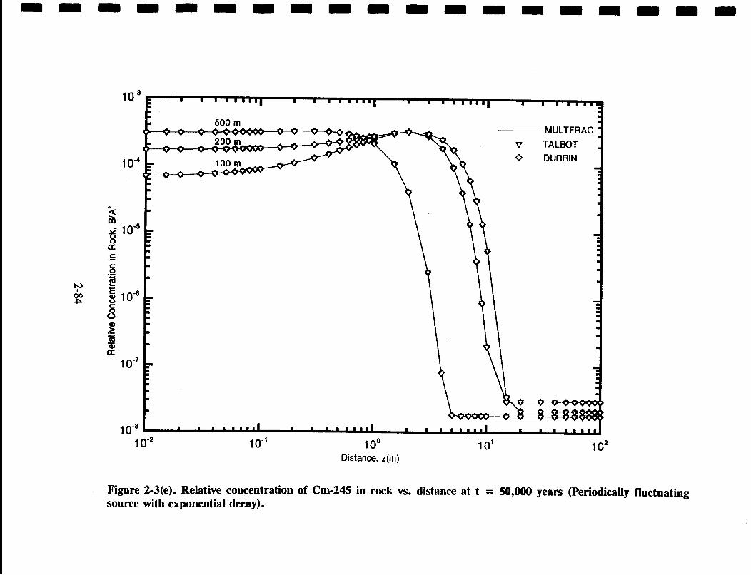
m m m m m m - m - m m - - m m m m -
10-3
10-4
s)
00
i 10-15
C
C:.0
aID 10o-8
CD 10-Ir1lo-,
0-8 I-1 -2 lo-, 100 10°
Distance, z(m)
102
Figure 2-3(e). Relative concentration of Cm-245 in rock vs. distance at t = 50,000 years (Periodically fluctuatingsource with exponential decay).

Table 2-12(a). CASE 2 RESULTS: CONCENTRATION OF Cm-245 IN THE ROCKMATRIX LAYER 2, AT DISTANCE x = 100 METERS AND TIME t = 50,000 YEARS(PERIODICALLY FLUCTUATING SOURCE WITH EXPONENTIAL DECAY ANDBAND RELEASE MODE)
DISTANCE z(m) MULTFRAC TALBOT DURBIN
1.000E-021.500E-022.OOOE-023.OOOE-024.OOOE-025.OOOE-026.OOOE-027.OOOE-028.OOOE-029.OOOE-021.OOOE-011.500E-012.OOOE-013.OOOE-014.OOOE-015.OOOE-016.OOOE-017.000E-018.OOOE-019.OOOE-011.0001E+OO1.500E+OO2.000E+OO3.OOOE+OO4.OOOE+OO5.OOOE+OO6.OOOE+OO7.OOOE+OO8.OOOE+O09.OOOE+OO1.000E+011.500E+012.OOOE+013.OOOE+014.OOOE+015.OOOE+016.OOOE+01
6.722E-056.833E-056.944E-057.166E-057.387E-057.608E-057.828E-058.048E-058.267E-058.486E-058.705E-059.791E-051.086E-041.296E-041.500E-041.695E-041.881E-042.058E-042.224E-042.379E-042.522E-043.046E-043.241E-042.811E-041.847E-049.587E-054.008E-051.366E-053.838E-069.069E-071.969E-072.967E-082.967E-082.967E-082.967E-082.967E-082.967E-08
6.722E-056.833E-056.944E-057.166E-057.387E-057.608E-057.828E-058.048E-058.268E-058.487E-058.705E-059.791E-051.086E-041.296E-041.500E-041.695E-041.881E-042.058E-042.224E-042.379E-042.522E-043.046E-043.241E-042.811E-041.847E-049.587E-054.008E-051.366E-053.838E-069.069E-071.969E-072.967E-082.967E-082.967E-082.967E-082.967E-082.967E-08
6.723E-056.834E-056.944E-057.165E-057.387E-057.607E-057.828E-058.048E-058.267E-058.486E-058.705E-059.791E-051.086E-041.296E-041.500E-041.694E-041. 880E-042.058E-042.224E-042.379E-042.522E-043.046E-043.241E-042.811E-041.847E-049.583E-054.002E-051.360E-053.823E-068.981E-071.995E-072.967E-082.967E-082.967E-082.967E-082.967E-082.967E-08
2-85
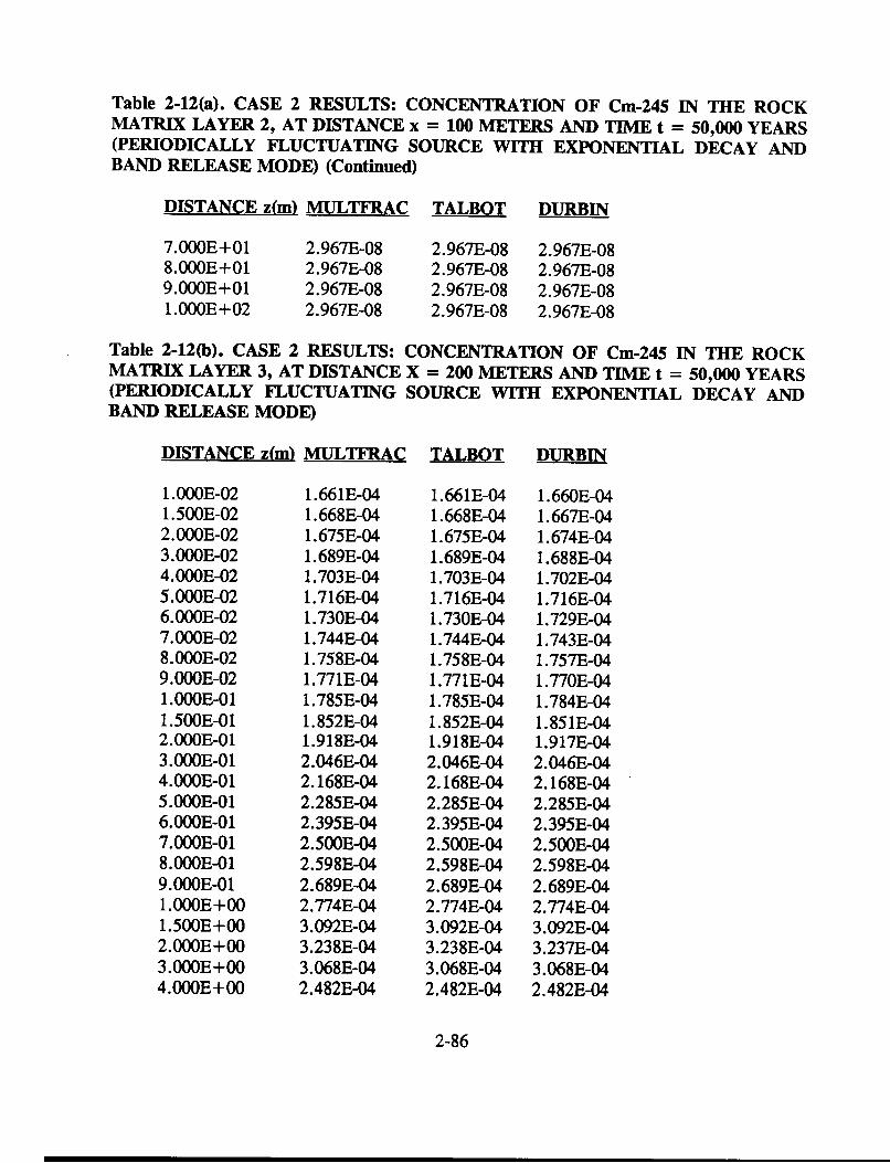
Table 2-12(a). CASE 2 RESULTS: CONCENTRATION OF Cm-245 IN THE ROCKMATRIX LAYER 2, AT DISTANCE x = 100 METERS AND TIME t = 50,000 YEARS(PERIODICALLY FLUCTUATING SOURCE WITH EXPONENTIAL DECAY ANDBAND RELEASE MODE) (Continued)
DISTANCE z(m) MULTFRAC TALBOT DURBIN
7.OOOE+018.OOOE+019.OOOE+011.OOOE+02
2.967E-082.967E-082.967E-082.967E-08
2.967E-082.967E-082.967E-082.967E-08
2.967E-082.967E-082.967E-082.967E-08
Table 2-12(b). CASE 2 RESULTS: CONCENTRATION OF Cm-245 IN THE ROCKMATRIX LAYER 3, AT DISTANCE X = 200 METERS AND TIME t = 50,000 YEARS(PERIODICALLY FLUCTUATING SOURCE WI1H EXPONENTIAL DECAY ANDBAND RELEASE MODE)
DISTANCE z(m) MULTFRAC TALBOT DURBIN
1.OOOE-021.500E-022.OOOE-023.OOOE-024.OOOE-025.OOOE-026.OOOE-027.OOOE-028.OOOE-029.OOOE-021.OOOE-011.500E-012.OOOE-013.OOOE-014.OOOE-015.OOOE-016.OOOE-017.000E-018.OOOE-019.OOOE-011.OOOE+001.500E+002.OOOE+003.OOOE+004.OOOE+00
1.661E-041.668E-041.675E-041.689E-041.703E-041.716E-041.730E-041.744E-041.758E-041.771E-041.785E-041.852E-041.918E-042.046E-042.168E-042.285E-042.395E-042.500E-042.598E-042.689E-042.774E-043.092E-043.238E-043.068E-042.482E-04
1.661E-041.668E-041.675E-041.689E-041.703E-041.716E-041.730E-041.744E-041.758E-041.771E-041.785E-041. 852E-041.918E-042.046E-042.168E-042.285E-042.395E-042.500E-042.598E-042.689E-042.774E-043.092E-043.238E-043.068E-042.482E-04
1.660E-041.667E-041.674E-041.688E-041.702E-041.716E-041.729E-041.743E-041.757E-041.770E-041.784E-041.851E-041.917E-042.046E-042.168E-042.285E-042.395E-042.500E-042.598E-042.689E-042.774E-043.092E-043.237E-043.068E-042.482E-04
2-86

Table 2-12(b). CASE 2 RESULTS: CONCENTRATION OF Cm-245 IN THE ROCKMATRIX LAYER 3, AT DISTANCE X = 200 METERS AND TIME t = 50,000 YEARS(PERIODICALLY FLUCTUATING SOURCE WITH EXPONENTIAL DECAY ANDBAND RELEASE MODE) (Continued)
DISTANCE z(m) MULTFRAC TALBOT DURBIN
5.OOOE+006.OOOE+007.OOOE+008.000E+009.OOOE+001.OOOE+011.500E+012.OOOE+013.OOOE+014.OOOE+015.OOOE+016.OOOE+017.OOOE+018.OOOE+019.OOOE+011.OOOE+02
1.755E-041.098E-046.129E-053.065E-051.378E-055.596E-063.477E-082.119E-082.119E-082.119E-082.119E-082.119E-082.119E-082.119E-082.119E-082.119E-08
1.755E-041.098E-046.129E-053.065E-051.378E-055.596E-063.477E-082.119E-082.119E-082.119E-082.119E-082.119E-082.119E-082.119E-082.119E-082.119E-08
1.755E-041.099E-046.131E-053.075E-051.371E-055.457E-063.477E-082.119E-082.119E-082.119E-082.119E-082.119E-082.119E-082.119E-082.119E-082.119E-08
Table 2-12(c). CASE 2 RESULTS: CONCENTRATION OF Cm-245 IN THE ROCKMATRIX LAYER 5, AT DISTANCE x = 500 METERS AND TIME t = 50,000 YEARS(PERIODICALLY FLUCTUATING SOURCE WITH EXPONENTIAL DECAY ANDBAND RELEASE MODE)
DISTANCE z(m) MULTFRAC TALBOT DURBIN
1.OOOE-021.500E-022.OOOE-023.OOOE-024.OOOE-025.OOOE-026.OOOE-027.000E-028.OOOE-029.OOOE-021.OOOE-011.500E-012.OOOE-01
3.001E-043.010E-043.019E-043.037E-043.054E-043.070E-043.086E-043. 100E-043.115E-043.128E-043.141E-043.194E-043.23 1E-04
3.001E-043.O1OE-043.019E-043.037E-043.054E-043.070E-043.086E-043. 100E-043.115E-043.128E-043.141E-043.194E-043.231E-04
3.001E-043.010E-043.019E-043.037E-043.054E-043.070E-043.085E-043. 100E-043.115E-043.128E-043.141E-043.194E-043.231E-04
2-87

Table 2-12(c). CASE 2 RESULTS: CONCENTRATION OF Cm-245 IN THE ROCKMATRIX LAYER 5, AT DISTANCE x = 500 METERS AND TIME t = 50,000 YEARS(PERIODICALLY FLUCTUATING SOURCE WITH EXPONENTIAL DECAY ANDBAND RELEASE MODE) (Continued)
DISTANCE z(m) MULTFRAC TALBOT DURBIN
3.OOOE-014.000E-015.OOOE-016.OOOE-017.OOOE-018.OOOE-019.OOOE-011.OOOE+001.500E+002.OOOE+003.OOOE+004.OOOE+005.OOOE+006.OOOE+007.OOOE+008.OOOE+009.OOOE+001.OOOE+011.500E+012.OOOE+013.OOOE+014.OOOE+015.OOOE+016.OOOE+017.OOOE+018.OOOE+019.OOOE+011.OOOE+02
3.254E-043.217E-043.125E-042.988E-042.814E-042.613E-042.393E-042.162E-041.083E-044.066E-052.598E-067.751E-081.832E-081.780E-081.780E-081.780E-081.780E-081.780E-081.780E-081.780E-081.780E-081.780E-081.780E-081.780E-081.780E-081.780E-081.780E-081.780E-08
3.254E-043.217E-043.125E-042.988E-042.814E-042.613E-042.393E-042.162E-041.083E-044.066E-052.598E-067.75 1E-081.832E-081.780E-081.780E-081.780E-081.780E-081.780E-081.780E-081.780E-081.780E-081.780E-081.780E-081.780E-081.780E-081.780E-081.780E-081.780E-08
3.253E-043.216E-043.126E-042.990E-042.814E-042.613E-042.392E-042.162E-041.083E-044.078E-052.599E-068.064E-081.833E-081.780E-081.780E-081.780E-081.780E-081.780E-081.780E-081.780E-081.780E-081.780E-081.780E-081.780E-081.780E-081.780E-081.780E-081.780E-08
2-88
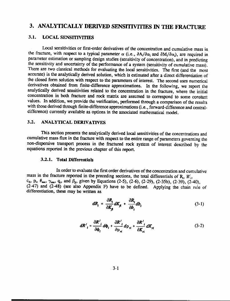
3. ANALYTICALLY DERIVED SENSMIVITLES IN THE FRACTURE
3.1. LOCAL SENSITIVITIES
Local sensitivities or first-order derivatives of the concentration and cumulative mass inthe fracture, with respect to a typical parameter a (i.e., MA1/aai and aMi/aat), are required inparameter estimation or sampling design studies (sensitivity of concentration), and in predictingthe sensitivity and uncertainty of the performance of a system (sensitivity of cumulative mass).There are two classical methods for evaluating the local sensitivities. The first (and the mostaccurate) is the analytically derived solution, which is estimated after a direct differentiation ofthe closed form solution with respect to the parameters of interest. The second uses numericalderivatives obtained from finite-difference approximations. In the following, we report theanalytically derived sensitivities related to the concentration in the fracture, where the initialconcentration in both fracture and rock matrix are assumed to correspond to some constantvalues. In addition, we provide the verification, performed through a comparison of the resultswith those derived through finite-difference approximations (i.e., forward-difference and central-difference) currently available as options in the associated mathematical model.
3.2. ANALYTICAL DERIVATIVES
This section presents the analytically derived local sensitivities of the concentrations andcumulative mass flux in the fracture with respect to the entire range of parameters governing thenon-dispersive transport process in the fractured rock system of interest described by theequations reported in the previous chapter of this report.
3.2.1. Total Differentials
In order to evaluate the first order derivatives of the concentration and cumulativemass in the fracture reported in the preceding sections, the total differentials of R,, R'i,Cf., Pi, O., -ya, qj, and Bji, given by Equations (2-5), (2-6), (2-29), (2-35b), (2-39), (2-40),(2-47) and (2-48) (see also Appendix F) have to be defined. Applying the chain rule ofdifferentiation, these may be written as
dR, MI a;dKfi + ab'Rdbi (3-1)
=aR aR aRdR', - aR' aRp s + ~(3-2)4i a~.Jpr + aKri
3-1

dAi = fideft af
+ abab,,
c'i dR ' +aR' X
acfi dDADP.
P.
(3-3)
d.i = P'-du, apa i+-da (3-4)
d8=' aadc, + 0 "dridO 8,^= 0 0t i
dym = ayndj+ mdra I T
(3-5)
(3-6)
(3-7)dq ,= - dc,jlcf
+ 'dR + dpi8-p
dpfi = aPid + aaCfl a
ardrJ = irdL,
f Mi i
PfidRi3Ri
apt+ Bfl dpiOi
+ duau.
(3-8)
(3-9)
(3-lOa)r, Ti, if < n
rs = in E u, i = n
substitution of Equations (3-3) and (3-9) in Equation (3-5) gives
(3-lOb)
3-2

dOM = ae fd1V+ ci db. + c'ft dl~il+a;Cflta 1 'ab, aRil a dD.I
(3-11)
+ (-1 ari i +3-duarit, i, I aUi i]
Similarly, substituting Equations (3-1) and (3-9) in Equation (3-6) yields
dy,,,= ay dR=aR.
+ "Y., Aid +C'j [8L,
Oi, duij (3-12)
where
du, = ab db,abi
(3-13)
Note that the total differentials of dR, and dR'i as given by Equations (3-1) and (3-2) are usedwhenever appropriate (i.e., if either Ri or R'j are expressed in terms of their respectivecomponents).
Using the following partial derivatives
ar, 1a_ = IaLi ui
(3-14a)
Lit i <j nL, = (3-14b)
X-Xi, i=n
ari fi
ao,,aCfl
(3-14c)
(3. 15a)
3-3

ao= (3-15b)
ay,
0 MR = r (3-16b)aRj
aq, _ CA
aCfl = q4R 52 (3-17a)
a-= 2 cfI + Pi (3-17b)aR, qi[2 Ri3 R 2J
aqf _ 2 (3-17c)op, q1R1
+ 2RJ ( j =1,2 (3-18a)
a,, cfl2R2 + pi j= 1,2 (3-18b)
__ - (-flyl, 2 j = 1,2 (3-18c)aq, 2
_ = _ _ =aq 1 (3-18d)pi aq, o-p, qjl
3-4

Opt (3-19a)
- = us (3-19b)
a'- 2b2 (3-20)ab. 21,2
the first order derivatives of O,., y , Cfi, R, and R'i with respect to a typical parameter ai arereported in Tables 3-1 through 3-5, respectively. Whereas the one corresponding to Oji givenby Equation (3-8) may be evaluated based on the latter tables and the various derivatives givenin Equations (3-14) through (3-20). Note that Q in Equation (3-20) corresponds to the steadyflow rate of water (Q = 2 uj be) through the fracture.
3.2.2. FIrst Order Derivatives of the Concentrations
Using the notations reported in Appendix D, the various components of Equation(2-42) may now be written as
F0 (xt) = AOet-'lPI, U(t - y 1 ) (3-21a)
for a continuously decaying source
,Hj(x,t) = e -A[bli Pn + (al - bl,) 3Pj,, 4Pjn 2P,.]U(t - y,,) (3-21b)
2
e= a2,. (-1y 9p Sp 7pU(t y) (3-21c)ji-
2
F,(x,t) = C laUE ( - y 9Pip lopih 11Phi-I (3-21d)
+ e-1t[bl, + (as,, - bl) P,, 6P.]
3-5

Table 3-1. FIRST ORDER PARTIAL DERIVATIVES OF 0. WITH RESPECT TO INPUTPARAMETERS a; (i.e., L;, u1, s, pi, Dp, Rt, Kf, R'1, and K; )
r, = j j� k. n; r, � q j, i -= n
NA = Not Applicablet Applicable if IDIST(2) = 1t Applicable if IDIST(2) = 0
3-6

Table 3-2. FIRST ORDER PARTIAL DERIVATIVES OF yL WITH RESPECT TOINPUT PARAMETERS ae (i.e., Li, u1, b1, A1, and Kfi )
l, i<n, n>1u1
Llj Rr,
_ i
L~~~~R
IDIS7T1)=0: Q i
IDIS711) = 1: -_K Sr + 2RIb,2 Q
Kfit r
r,=1ij, i<n; r1= %, i=n
t Applicable only if IDIST(1) = 1Applicable only if IDIST(1) = 0
3-7

Table 3-3. FIRST ORDER PARTIAL DERIVATIVES OF Cfi WITH RESPECT TO INPUTPARAMETERS ai (i.e., L,, ui, O;, pi, D>, RI, Kfi, R'k, AND K,;)
E .00 fff000 ffff:00 0000. .:ffV:--fff 0 ;;0C:: - '-R '. ::'V" 'S fffffffffffffffffffff :'t" ,..,,,. ..,. .........._ . ..LiD t NA Dpi cJN
2D.pi
Ui ~~NA liNA
bi cfl ~~~~~Kfi NA
IDISY(2) =0: C R CAl0, ~~~~~~~~2 R'i
IDIS7(2) = 1: 0| 2,R' |
Pit CflKl__*t l, C2i( 1
NA = Not Applicablet Applicable only if IDIST(2) = 1t Applicable only if IDIST(2) = 0
3-8
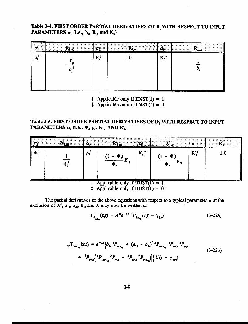
Table 3-4. FIRST ORDER PARTIAL DERIVATIVES OF Ri WirM RESPECT TO INPUTPARAMETERS oj (i.e., b;, RA, and K,;)
t Applicable only if IDIST(1) = 1* Applicable only if IDIST(1) = 0
Table 3-5. FIRST ORDER PARTIAL DERIVATIVES OF R'i WiTH RESPECT TO INPUTPARAMETERS ci (i.e., i, pi, K. AND R',)
_ 1 P(__Pi (lYn)t Rii 1.0
-(I -rrtoplic e onlv if : f L)) = 1 Pr1
____ ____________-t Ainnicable onlv if IDIST( I i=- I
t Applicable only if IDIST(1) = 0.
The partial derivatives of the above equations with respect to a typical parameter a at theexclusion of A', ali, a21, b1i and X may now be written as
FO (xt) = A&e - t 1Pl,, U(t - Y1)
- [ ~~~3p. t 4p. 2pMHL,,,, (xt) lb= e {b 1Pm,, + (ali - bl) ,m.
+ 3 p( 4 pi 2 p + 4 Pi 2 p )]}U(t - y
(3-22a)
(3-22b)
3-9

2Hf, (X~t) =eCta-t E (_ W) 9 P 8 P 7 P2 Hin,( ' =Ieaj if J4, Jim] jim- a
8p.. 7 P~' + jfnjt"]UOt
(3-22c)
2F (xt) = e -Ata 2 .; E (-1)y [ 9 P,( 10Pf 11PJ, + lOPj3 1 1p )J=1~~J lp U lp1 + 9 p. lop; HP.n
I,nu in in]
+ e t pb + (a,, - bl')( 5 P... 6pj + 5P. 6p.)]
(3-22d)
the first order partial derivatives of the functions given by Equations (3-21) with respect to Al,ali, a2i, and b1i may now be written as
F. (xt) = e -At lp IU(t - y 1 )
Fo (xt) = - t F (xt) U(t - Y 11)
,Hf,.,,,(x,t) = e;t[ 3Pi, 4pi,,,,,. 2 Pma,]U(t - yn,)
,Hi,,.,,,,(X,t) = -t lH,,,,(x~t) U(t - yj"
(xt) = e -t[ lP _ 3p- 4p 2p u(t - Yj
2Hfhut(Xs) - 2H2,(Xt) U(t-Ym,,)
2 H,%,, (X,t) = -t H,,, (Xt) U(t -Y.l,,)
(3-23a)
(3-23b)
(3-24a)
(3-24b)
(3-24c)
(3-25a)
(3-25b)
3-10

Fn (xt) = e -At 5P' 6P. (3-26a)
F,, = e Xt (-1y 1 0 p lip 1 (3-26b)
Fn,(xt) = 1 - e 1At[ Sp, 6p,] (3-26c)
F,, (x,t) = -t F((X~t) (3-26d)
3.2.3. First Order Derivatives of the Cumulative Mass
Using the notations reported in Appendix E, the various components of Equation(2-62) may now be written as
Q(x, t) = AO{ G 'G1 +[ 3G G , 2G ,+ 3G - 2Gbn]) U(t-ymn) (3-27a)
for a continuously decaying source
b11{~OG1G~2G, 3G1,, + 2GZ 3G,;,4 U(t-y,,)IQInn(xt) = blj{- °G tG+ 2G,, G,,, G~ Gm}~ty)(3-27b)
+(a .bl) { 7G.6G. 5 G. - 3 G+ 2 G 4 Gi- + 3 G 2G,-n 4Gij} U(t - Y.,)
2
2Qj(Xlt) = a2 (-1{ 0 Gfi 9 G 1 4 Gi 'G, (3-27c)
OGJ,(- 3G;, 2 G,, 1 1G7 + 3 G,, 2 G,;j lGi+)} U(t-y,,,)
2= a,,~j(-1Y~{ 0G 14j4 12GJ 13Gjn + jn,,( 16GJ-1j-1
3-11
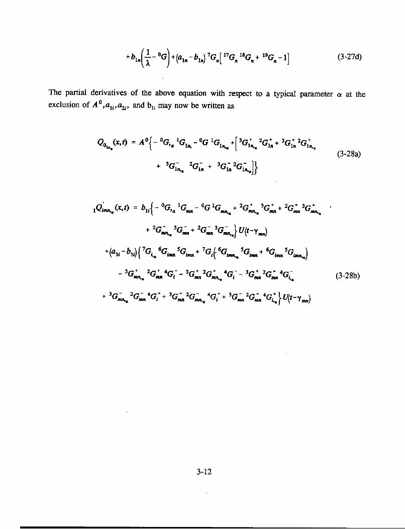
+ b( OG) + (a,. - bI.) 7GR[ 17Gn "gGn + 19GB - 1] (3-27d)
The partial derivatives of the above equation with respect to a typical parameter a at theexclusion of A 0 ,a 1 j,a2i, and b1i may now be written as
QO(x,t) A o{f- 1G, 'GI, - °G 1G,. +[ 3Gl 2G1 + 3G + 2G +(3-28a)
+ 3Gc, 2G- + 3G - 2G-,,j}
,(t)= b{- OGx 1Gm - °G 1'G + 2G 3G+ 2G 3G;
+ 2G,-7m 3G,-, + 2 G 3G,},,,, } U(t-y,,,)
+ (a1f - b1 ){ 7G46G,, 5G1 . + 7GL(. 6Gbm,, 5Gf + 6Gn 5GL,)
3G,~. 2GL 4G - 3G, 2G,m,, 4G% - 3G;3 2GL 4G- (3-28b)
+ 3G,;,. 2G-;a 4G + + 3 G; 2G,,, 4G + 3 Gz 2G; 4GC -U(tYmn)
3-12

2
2Qm,.(xt) = a2i 2 (-1Y{ G.. 'G.. L fi'4Gj J0G 14i]j-1 ft6 ,~~L.. Li + jLi. Gi.] +
I0Gft14 GSi[9 Gj, 8 G . + G. ,]
- '0 G [3GL 2 G; 11G;f - 3Gma 2Gm, 1Gj]
lOGji[3G+ 2GI+ 1G; + 3Gm 2G IG m n m2 11GJZ (3-28c)
-3G^. 2Gzn1IG,-3G 2GmF 1 G+-3G- 2G- IIG+j, _Y.
2
Qn (x,t) = a2^ E (- lY [ IG 14G + 10G "j4G L 1"]2Gi-i
10GJ 4Gj4 12G 1 3G 2 13G +G , + 1 1G,( GM ) + j 16G,]
+bln( A , - OG,,+(a,-b,.) [7GnJ ,,, (17Gn 18Gn + 19G, -1) (3-28d)
+ 7 Gn (17 G, 18G X+ 17G,, 18Gn + 19G0 )]
The first order derivatives of the equations given by Equations (3-27) with respect to parametersA-, ali, a2i, and bli are given by
Q0 (x,t) = -Q (xst) U(t - Yip) (3-29)1 (x = ,I& - A 01,,
IQ' 41 i .(X,t) - 7Gi 6Gima 5G. - 3cc,, 2GpI 34G[-+ 3G,;UI 2GL~, 4G1+} u(t - YMa) (3-30a)
3-13

lQi.^i (xI) = {- G 1G , + 2GJ 3Gj + 2G- 3G-} U(t )
-{ Gi IGi,, lGi. - 3G. 2GL GiG + 3G" 2Gm 4G.~} U(t -y.)
2Q 'b,, (x, t) =- 2Q i,,,(Xt) U(t - y)
Q.,(x,t) = 7 G,,[ 17G, 18G, + 19Gm - 1]
(3-30b)
(3-3 1)
(3-32a)
Qn, (x t) =
2
iS (-lY{ '0 Gjn jnG, 12Gjn i3 Gjn + j5Gn( 16 G 1)]}j-l 'in
(xt) = 1 - °G - 7G,, [ 17G,, 18G,, + 19G,, - 1]
(3-32b)
(3-32c)Q14bjXI
3.3. NUMERICAL DERIVATIVES
The numerically derived derivatives are based on the parameter perturbation technique(see Becker and Yeh, 1972), which uses forward or central difference schemes. In suchinstances, the choice of the step size (or perturbation vector) usually has an important bearingon the choice of the particular scheme. The investigator is commonly confronted with theproblem of deciding upon the magnitude of this parameter, which is generally selected by meansof a trial-and-error procedure.
The forward-difference approximation (FDA) is given by
qfAA),J(A + h) -AfA) + O(h)ah h
(3-33)
and the central-difference approximation (CDA) is given by
afA) _A + h) - f(A - h) + O(h2 )ah h
(3-34)
3-14

where h is the step size. Ideally, the step size should be small enough to reduce the truncationerror and large enough to cause a reasonable change in the significant figures of vector A.Following Bard (1974), we write
h =e A
where 10-5 < E < 10-2.
Recently, Dennis and Schnabel (1983) recommended setting e equal to the square rootof the relative computer precision, which in our case corresponds approximately to 10-16. Notethat for a typical parameter, N + 1 evaluations of the response vector are required at eachiteration by the FDA (compared to 2N + 1 evaluations in the case of CDA), where Ncorresponds to the number of observation points.
3.4. VERIFICATION
The verification of the analytically derived local sensitivities was performed bycomparison of the results yielded by this solution scheme with the ones obtained through the twofinite-difference appproximations discussed earlier. The exact derivatives as well as the onesyielded by FDA and CDA were estimated, based on the data presented in Table 2-1 and valuesof e corresponding to 10-16. Figures (3-1) and (3-2) illustrate the sensitivity of the concentrationand cumulative mass of Np-237 in the fracture to a selected choice of parameters (i.e., b, DP,Kf, and Kr) in each of the five fracture layers. At the exception of the very low range ofsensitivities, the numerical results are in excellent agreement with the analytical ones. Note thatthe values obtained from both FDA and CDA methods were identical for all the investigated testcases, when the selected values of e are less than 10-2. A detailed examination of thesensitivities will be presented in Part 2 of this report.
3-15

3.0E-2
I -6.5E-9
~ 3.0OE-2
An*_ta
a~-6.02-2
-9.OE-2103 104 1og
Time (yews)
Figure 3-la. Sensitivity of concentration to half-thickness vs. time for Np-237.(Exponentially decaying source).
0 2.5E-1
,-7.5E-8
-2.5E-1
> o Numerica~~~~~~~ayrLayer 15 -5.0E-1 Layer 3o ~~~~~~~Layer 4
-7.52-1 Lae ___Analytical
o rWkmerical
l -. OEO
103 104 o1Time (years)
Figure 3-lb. Sensitivity of concentration to pore diffusivity vs. time for Np-237.(Exponentially decaying source).
3-16

0
U.
n0
0
t=feii0
C
0U8
:t:
-0
-9.OE-2 L-Io3 10'
Time (years)1 05
Figure 3-ic. Sensitivity of concentration to surface distribution coefficient in fracture vs.time for Np-237 (Exponentially decaying source).
1 .OE-2
.' 5.6E-9
E0
-1 .OE-2.a0
A -2 .OE-2S
o -4.OE-2(.,
a -5.OE-2
-6.OE-2 L1o3 104
Time (years)105
Figure 3-id. Sensitivity of concentration to distribution coefficient in rock vs. time forNp-237 (Exponentially decaying source).
3-17

-5.OEO
-1.0E1 La 1
e -1.5E laye /
O -2.OE1 Layer 3
c' -2.5E1 Layer Analytical0 Numerical
-3.OE layer
10 31o
405 06
Time (years)
Figure 3-2a. Sensitivity of cumulative mass to half-thickness vs. time for Np-237(Exponentially decaying source).
O O.OEO
2',
-2.5E2
a. -5.0E2 Laera
Layer 2
lii \ \ Xo ,# AnalyticalES Layer 4 0 Numerical
*t -7.5E2 \ g7.5E2
103104 1
Time (years)
Figure 3-2b. Sensitivity of cumulative mass to pore diffusivity vs. time for Np-237(Exponentially decaying source).
3-18
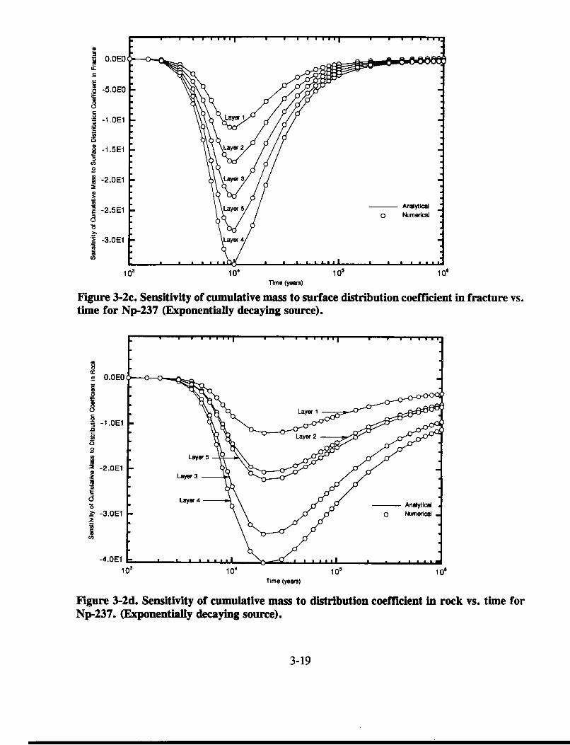
0
0 .OEO~CU-
g -5.OEO
SZ -I.OE1.0E -1.5E1r
0
1 -2.OEl0
E -2.5Ela
'5 -3.OE1Q)CDco
103 104 105 10'
Time (years)
Figure 3-2c. Sensitivity of cumulative mass to surface distribution coefficient in fracture vs.time for Np-237 (Exponentially decaying source).
sO.OEO
j -1.OE1i
2 Layer s2.OEILayer 3
E. Layer 416 An f talytical= -3.OE1 o t& ° merical
-4.OE1103 10
4WOs 10l
Time (years)
Figure 3-2d. Sensitivity of cumulative mass to distribution coefficient in rock vs. time forNp-237. (Exponentially decaying source).
3-19

4. CONCLUSIONS
Analytical solutions based on the Laplace transforms have been derived for predicting the one-dimensional non-dispersive isothermal transport of a radionuclide in a layered system of planarfractures coupled with the one-dimensional infinite diffusive transport into the adjacent rockmatrix units. The solution for the cumulative mass in the fracture has also been reported.
The particular features of these solutions reside in their analytical capability designed to handle:
(a) residual concentrations in both fracture and rock matrix layers respectively. Thelatter are represented by a constant and/or a spatially dependent function in thecase of the fracture, and a constant, in the case of the rock matrix,
(b) layered nature of the rock mass,
(c) length dependency of fracture aperture yielding a non-uniform velocity field, and
(d) both exponentially decaying and periodically fluctuating decaying source ofsolute at the upstream end of the fracture network, which may then be subjectto either a step or band release mode.
The reported analytical solutions pertaining to the concentrations and cumulative mass weresuccessfully verified by means of three reliable numerical methods for evaluating the inverseLaplace transform in the real and complex domain respectively. To this end, two test casesinvolving the migration of Np-237 and Cm-245 in a five-layered fractured rock system, usingsynthetic, but realistic data, were investigated. The calculated analytical local sensitivities ofnuclide concentration and cumulative mass flux in fractures with respect to all of the modelparameters were in excellent agreement with the ones obtained through a finite-differencemethod of approximation. In this particular instance, no marked evidence of a superiorperformance of the central over the forward finite-difference method was found as theorysuggests.
In spite of some limitations (i.e., assumptions of zero dispersion in the fracture and infinitematrix diffusion), the new features embedded in the reported solutions, which allow one to dealwith layered media having piece-wise constant properties, as well as non-zero initial conditions,coupled with a realistic option of a periodically fluctuating decaying source, render thesesolutions very useful and, above all, cost effective for performing sensitivity and uncertaintyanalyses of scenarios likely to be adopted in performance assessment investigations of potentialnuclear waste repositories.
4-1

5. REFERENCES
Ahn, J., P. L. Chambrd, and T. H. Pigford. 1986. Radionuclide migration throughfractured rock: effects of multiple fractures and two-member decay chains. EarthSciences Division, Lawrence Berkeley Laboratory and Department of NuclearEngineering, University of California, Berkeley, CA.
Ahn, J., P. L. Chambrd, and T. H. Pigford. 1985. Nuclide migration through a planarfissure with matrix diffusion. LBL-19249, Lawrence Berkeley Laboratory andDepartment of Nuclear Engineering, University of California. Berkeley, CA.
Bard, Y. 1974. Nonlinear parameter estimation. Academic Press. New York, NY.
Becker, L., and W-G. Yeh. 1972. Identification of parameters in unsteady open channelflows. Water Resour. Res. Vol.8, No.4, pp. 956-965.
Bear, J., 1972. Dynamics of Fluids in Porous Media, American Elsevier Publishing Co.,New York, NY.
Burkholder, H. C., M. 0. Cloninger, D. A. Baker, and G. Jansen. 1976. Incentives forpartitioning high-level waste. Nuclear Technology, Vol. 31, p. 202.
Chambrd, P. L., T. H. Pigford, A. Fujita, T. Kanki, A. Kobayashi, H. Lung, D. Ting,Y. Sato, and S. J. Zavoshy. 1982. Analytical performance models for geologicrepositories. Vol. II, LBL-14842. Lawrence Berkeley Laboratory, University ofCalifornia. Berkeley, CA.
Chen, C. S. 1986. "Solutions for radionuclide transport from an injection well into asingle fracture in a porous formation." Water Resources Research. Vol. 22, No.4, pp. 508-518.
Dennis, Jr., J.E., and R. B. Schnabel. 1983. Numerical methods for unconstrainedoptimization and nonlinear equations. Prentice Hall, Englewood Cliffs, NJ.
Durbin, P. 1974. Numerical inversion of Laplace transforms: an efficient improvementto Dubner and Abate's method. Comp. J. 17, 371-376.
Foglia, M., F. Iwamoto, M. Harada, P. L. Chambrd, and T. H. Pigford. 1979. "TheSuperposition equation for the band release of decaying radionuclides throughsorbing media." UCB-NE-3335, University of California at Berkeley. ANSTransactions. Vol. 33, pp. 384-386.
5-1

Grisak, G. E., and J. F. Pickens. 1981. "An anlaytical solution for solute transportthrough fracture media with matrix diffusion." Journal of Hydrology. Vol. 52,pp. 47-57.
Grisak, G. E., and J. F. Pickens. 1980(a). "Solute transport through fractured media,1. The effect of matrix diffusion." Water Resour. Res. 16(4): 719-730.
Grisak, G. E., Pickens, J. F., and J. A. Cherry. 1980(b). "Solute transport throughfractured media, 2. Column study of fractured till. " Water Resour. Res. 16(4):731-739.
Gureghian, A. B. 1990a. FRACFLO: Analytical solutions for two-dimensional transportof a decaying species in a discrete planar fracture and equidistant multiplefractures with rock matrix diffusion. BMI/OWTD-5, p. 244. Office of WasteTechnology Development, Battelle. Willowbrook, IL.
Gureghian, A. B. 1990b. FRACVAL: Validation (nonlinear least squares method) of thesolution of one-dimensional transport of a decaying species in a discrete planarfracture with rock matrix diffusion. Part 1: Analytical solutions. BMI/OWTD-8,p. 79. Office of Waste Technology Development, Battelle Energy SystemsGroup, Willowbrook, IL.
Gureghian, A. B. 1987. Analytical solutions for multidimensional transport of a four-member radionuclide decay chain in ground water. BMI/OCRD-25, p. 162.Office of Crystalline Repository Development. Battelle Memorial Institute.Columbus, OH.
Gureghian, A. B., and G. Jansen. 1985. "One-dimensional analytical solutions for themigration of a three-member radionuclide decay chain in a multilayered geologicmedium." Water Resources Research. Vol. 21, No. 5, pp. 733-742.
Gureghian, A. B., and G. Jansen. 1983. LAYFLO: A one-dimensional semi-analyticalmodel for the migration of a three-member decay chain in a multilayeredgeologic medium. ONWI-466, p. 87. Office of Nuclear Waste Isolation, BattelleMemorial Institute, Columbus, OH.
Hadermann, J. 1980. "Radionuclide transport through heterogeneous media." NuclearTechnology. Vol. 47, pp. 312-323.
Hodgkinson, D. P., and P. R. Maul. 1985. One-dimensional modelling of radionuclidemigration through permeable and fractured rock for arbitrary length decaychains using numerical inversion of Laplace transforms. AERE-1 1889. AERE-Harwell, Oxfordshire, UK. p.36.
5-2

Kanki, T., A. Fujita, P. L. Chambrd, and T. H. Pigford. 1981. Transport ofradionuclides through fractured media. UCB-NE-4009. Lawrence BerkeleyLaboratory, University of California, Earth Sciences Divison. Berkeley, CA.
Neretnieks, I. 1980. "Diffusion in the rock matrix: An important factor in radionuclideretardation?" Journal of Geophysical Research. Vol. 85, pp. 4379-4397.
Piessens, R. and R. Huysmans. 1984. Algorithm 619: Automatic numerical inversion ofthe Laplace transform. ACM Trans. Math. Softw., 10, 3, pp. 348-353.
Pigford, T. H., P. L. Chambrd, M. Albert, M. Foglia, M. Harada, F. Iwamoto, T.Kanki, D. Leung, S. Masuda, S. Muraoka, and D. Ting. 1980. Migration ofradionuclides through sorbind media analytical solutions - II. Vol. II, ONWI-360(2), LBL-1 1616. Lawrence Berkeley Laboratory. University of California atBerkeley.
Rasmuson, A. and I. Neretnieks. 1986. "Radionuclide transport in fast channels incrystalline rock." Water Resources Research. Vol. 22, pp. 1247-1256.
Rosinger, E. L. J. and K. K. R. Tremaine. 1978. GARD2 computer program for thegeochemical assessment of radionuclide disposal. AECL-6432, Atomic Energyof Canada. Whiteshell Nuclear Research Establishment.
Shamir, U. Y. and D. R. F. Harleman. 1966. Numerical and analytical solutions ofdispersion problems in homogeneous and layered aquifers. MIT Report No. 89,p. 206. Massachusetts Institute of Technology. Cambridge, MA.
Stefhest, H. 1970. "Numerical inversion of Laplace transforms." Commun. ACM. Vol.13, No. 1, pp. 47-49.
Sudicky, E. A., and E. 0. Frind. 1982. "Contaminant transport in fractured porousmedia: Analytical solution for a system of parallel fractures" Water ResourcesResearch. Vol. 18, No. 6, pp. 1634-1642.
Sudicky, E. A. and E. 0. Frind. 1984. "Contaminant transport in fractured porousmedia: Analytical solution for a two-member decay chain in a single fracture"Water Resources Research. Vol. 20, No. 7, pp. 1021-1029.
Talbot, A. 1979. The acurate numerical inversion of Laplace's transforms. J. Inst. Math.Applics. Vol. 23, pp. 97-120.
Tang, D. H., E. 0. Frind, and E. A. Sudicky. 1981. "Contaminant transport infractured porous media: Analytical solution for a single fracture" WaterResources Research. Vol. 17, No. 3, pp. 555-564.
5-3

van Genuchten, M. Th., and W. J. Alves. 1982. Analytical solutions of the one-dimensional convective-dispersive solute transport equations. U. S. Departmentof Agriculture, Technical Bulletin No. 1661.
5-4
APPENDIX A
THEOREMS AND LAPLACE TRANSFORMS

In this appendix, a selected number of theorems and inverse Laplace transforms are reported(Abramowitz and Stegun, 1972).
A.1. THEOREMS
The operations for the Laplace transformation reported in this report require, in somecases, the use of the following theorems. Note that f(s) corresponds to the Laplace transform offunction F(t).
A.1.1. Translation
L -I I e -bsAs) I = F(t - b) U(t - b),b>O (A.l-1)
where U(t) is the Heaviside unit step function defined as
0, t<O
U(t) = 2,t = 0 (A.1-2)
1, t>O
A.1.2. Linear Transformation
L -l'[s - a)] = eaF(t)
A.1.3. Differentiation
L -sJ~s) - F(+O) = F(t)
L-sRAs) - Lls 1 F(+O)-L-lsn-2F'(+O)-...-F(n-1)(+O) =F Pn(t)
A.1.4. Convolution or Faltung
t
L[ t(s)f2(s)] = fF1 (t - r)F2(¶)ds = F1*F20
(A.1-3)
(A.1-4)
(A.1-5)
A-1

In the following, the Laplace transform of the function on the right is given on the left-hand side.
Table A.1. LAPLACE TRANSFORMS
A-2

The inverse Laplace transform of the product of l/(s2 + a2) and e-a4' may be obtained using theirrespective inverse transforms given in Table A. 1 and applying the convolution theorem, Equation(A.1-5), to yield
A-3

s -aib
t ~~a 2
a e~b~t - ") e ds2 Fo rI312
aeibt 1 - - a2
= ae +re dr(A.2-1)
itt a 22 ibae- b f e I C2
U t-t2
Using the integral given by Equation (C-1) we get
L-1 e-aVSS2 + b2
=L-1 e-a[ 1 1 I2ib sT -ib s + ib]
(A.2-2)
= -I[E(tsaib) - E(tsa,-ib)]4ib
where
E(tAib) =e(I-eaVIerfc(A +i)+ e -aVlea f a _ tJ
Substituting for Vi in Equation (A.2-3) using the following relations
(A.2-3)
V = (e(,,12 = coeS'4
+ isin = 1 +i4 2
(A.2-4)
yields
A-4

E(t,4b) =e a() + ib+a4(Ž )tJerf4 . +(2)* +(2)|
(A.2-5)
+ex4-a(b) + tbo) f ai
A similar expression to the above may be obtained for E (t, a, -ib) after substituting for V-i thefollowing relation
= (e (,1T = 1 - (A.2-6)
Hence
E(t~ab) - E(ta -ib) =
exp(A + iB)erfc(C + iD) - exp(A - i)erfc(C - iD) + (A.2-7)
exp(A + iB)erfc(C + iD) - emp(A - iRcerfc(C - iD)
where
A a 2; B =bt + a(2); C= a 4 j (2; D 2
A (b~l2 (2~l C Vt- 2 2b (A.2-8)
1= -a(bf)-5; A tm-a(b)-; a _5 (btyh.j; =5 _b,-
A-5

APPENDIX B
EVALUATION OF ERROR FUNCTION AND PRODUCT OF EXPONENTIAL ANDCOMPLEMENTARY ERROR FUNCTION TERMS

B.1. Error Function
The error or probability function is defined as
erflx) = 2 f e 2d&dIo
with
erj-x) = -erAx)
this may be expressed in terms of the complementary error function erfc(x) written as
edrfx) = 1 - erfc(x)
(B.1-1)
(B.1-2)
(B.1-3)
where
W
erfc(x) = 2 Jfet2 dt=x
erfc(-x) = 2 - eifc(x)
(B.1-4)
and
(B.1-5)
Note that when x is small the integrand in Equation (B.1-1) may be conveniently expanded ina power series convergent everywhere and integrated term by term to yield
erflx) = 2 x3XS X7
5-21 7 31(B.1-6)
+ (_l)n~l X + |.
(2n+1) *nI
A few terms in the expansion are necessary to determine the value of erf(x) to a givennumber of decimal places. However, as x becomes large, the loss in accuracy must becompensated by a large number of terms which renders the calculation tedious and impractical.A rational Chebysheb approximation may be used to alleviate this problem when x 2 4 (seeCody, 1969). Alternatively, the asymptotic expansion reported by Abramowitz and Stegun (1972)
B-1

expressed in terms of the complementary error function. erfc(x) (see Equation (B.2-3)) is used.
The derivative of the error function may be written as
d[erflx)] =2 exp(-x2) dx (B.1-7)da :/ du
B.2. Formulae of Error Functions with Complex Arguments
Let z be the complex argument written as
z = x iy (B.2-1)
and Euler's formula written as
et = cosz + isinz (B.2-2)
Note that the evolution of the error function for a real argument was based on Cody (1969).
B.2-1. Asymptotic Expansion I z I > 2 and x < 1 and I y I 2 6
In this case, the asymptotic expansion of erfc(z) as given byAbramowitz and Stegun (1972) may be written as
erfc(z) = 6 1 + 1.3... (2n- 1)1 +
Zs/ 1 n-i (2z) J
(B.2-3)where R (x) is the remainder after n terms.
B.2-2. Confluent Hypergeometric Function I z I < 2
In this case, the error function is evaluated from the confluent hypergeometric function(see Abramowitz and Stegun (1972) Equation (7.1.21), written as
erfz = 2ZM(1,3,_z2) = 2Ze-Z 2M(1 3 z2) (B.2-4)
whe 22 '2'
where M is the Kummer's function (see Abramowitz and S tegun (1972), p.504, Equation
B-2
(13.1.2)), written as
M(a, b,z) =1+ az+ (a 2z (a) + zb Wb22f (b),,nl
with
(a)n = a(a + 1)(a + 2) *.. (a + n - 1), (a), = 1
B.2-3. Continued Fraction Approximation I z I > 2 and x > 1
(B.2-5a)
(B.2.5b)
In this case, the error function is evaluated from the continued fractions approximations(see Abramowitz and Stegun (1972) p.298, Equation (7.1.14)), written as
eez2 1 1/2 1 3/2 2erfc (z) =-z +z +z ... (Rz> 0) (B.2-6)
B.2-4. Infinite Series Expansion I z I >2,0<x< 1,y<6
In this case, the eror function is evaluated from the infinite series approximation (seeAbramowitz and Stegun (1972), p. 299, Equation (7.1.29)), written as
erf(x + iy) = erx + e2 [(1 - cos 2xy) + isin2xy]2inx
(B.2-7)
+ 2 e-X2 i
71 n -l n2+ 4X2 [f,(XxY) + iag(XsY)] + E(Xy)
where
f.(x,y) = 2x - 2xcoshnycos2xy + nsinhnysin2xy (B.2-8a)
gn(xy) = 2xcoshnysin2xy + nsinhnycos2xy (B.2-8b)
e(x,y)I a 10-1 61erf(x + iy)I (B.2-8c)
B-3

B.3. Evaluation of Product of Exponential and Complementary Error Function withComplex Arguments
Functions involving the product of exponential and complementary error functions maywitness two types of arguments inherent to such functions, i.e., real or complex.
When the arguments of the exponential and complementary functions are both real, thescheme reported in Appendix C of Gureghian (1990) is the one adopted in this work. However,in the event where the arguments of these functions are of the complex form, the typical modelfor the complementary error function as reported in the preceding sections is selected based uponits adequacy to cope with the magnitude of the complex argument of interest. In the case wherean infinite series approximation model for the complex error function, such as given by Equation(B.2-7) is adopted, it will be subsequently shown that expressions similar to one given byEquation A.2-7, which display a combination of products of complex exponential andcomplementary error functions, may yield either a real or an imaginary number.
Writing
F+(t,A,iB,C,iD) = exp(A + iB)erfc(C + iD) (B.3-1)
+ exp(A - iB)erfc(C - iD)
and using Equations (B.2-2) and (B.2-7), it may be shown that the result is a real number givenby
F +(tAiBC4D) = 2exptA)[cosB (erfc(C) -
u(C) (1 - cos2CD) - v(C) r. (C) fn (CD)
( - ~~~~~~~~~~~~(B .3-2)+ sinB u(C)sin2CD + v(C) Q r. (C)g.(CD)
+ C(ABCD)
Similarly, writing
F-(t,A,iB,C,iD) = exp(A + iB)erfc(C + iD) (B.3-3)
- ep(A - iB)erfc(C + iD)
B-4

it may be shown that the result is an imaginary number given by
F-(t,A,iB,C,iD) = i2exp(A)[ sinB(e*c(C) -
u(C)(l - cos2CD)- v(C)E r,(C)f,(CD)I
- cosB(u(C)sin2CD + v(C)i r,(C) g8n(C9D))j (B.3-4)
+ e(AB,CD)
where
U(C) e (B.3-5a)2nrC
_2e c 2v (C) = 2e(B.3-5b)
7T
n2
(C) e (B.3-5c)n+ 4C2
and f., g. and £ are given by Equations (B.2-8a) through (B.2-8c).
Equations (B.3-2) and (B.3-4) may be written in a more explicit form as
B-5

F+(t,A~iB,CiD) = 2[cosB exp(A)erfc(C)
+ exp(A. - C [ - cosB + cos(B - 2CD)]
r2 _ _ I7r.. f 2 C2 [n [E2 - E3]sin(B - 2CD)
(B.3-6)
+ 2C( El cosB - cos(B - 2CD)[E2 + E3])
F - (tA,iBCiD) = 2i [sinB exp(A)erfc(C)
+ exp(A - C 2[ - sinB + sin(B - 2CD)]27cC
n 2 n 2 + C2 [n [E2 - E3]cos(B - 2CD)(B.3-7)
+ 2C(E, sinB - si(B - 2CD)[E2 + E3])]
where
E 1 = exp(A - C 2 - n)4
(B.3-8a)
E2 =ep(A - C2 - - + nD)4
(B.3-8b)
(B.3-8c)E, = 2 ep(A _C 2 _ - _nD)4
B-6

REFERENCES:
Abramowitz, M., and I. A. Stegun. 1972. Handbook of Mathematical Functions. DoverPublications, Inc., New York, NY.
Cody, W. J. 1969. Rational Chebyshev Approximation for the Error Function. Mathematics ofComputation. Vol. 23, No. 107, pp.631-637.
Gureghian, A. B. 1990. FRACVAL Validation (Nonlinear Least Squares Method) of the Solutionof One-Dimensional Transport of Decaying Species in a Discrete Planar Fracture withRock Matrix Diffusion Part 1: Analytical Solutions. BMI/OWTD-8 Battelle EnergySystems Group, OWTD, Willowbrook, IL.
B-7

APPENDIX C
SOME INTEGRALS INVOLVING THE ERROR FUNCTION AND OTHERFUNCTIONS

This appendix reports the derivation of a number of integrals involving products of exponentialand complementary error functions which are required for an exact evaluation of the cumulativemass flux presented in section 2.3.
From Abramowitz and Stegun (1972) (p.304, Eqn. 7.4.33), we have the following indefiniteintegral:
_a2X2_ b2
fe 2 dx = -FN[e2aberf(ax + b) + e 2aberax - b), (a o)4a[ x X(C.1)
C.1.1Writing
I1(t,cC,Y) = fel e* ey)112f
Integrating this equation by parts gives
Il(tlaPy) = I11 + 112
where
(C.1-1)
(C.1-2)
'11 = _(t - y) 112
a12 = - / 2feL ( T YY) d[ . 12j
(C.1-3)
(C.1-4)
W e Y& t-Y'12 = f
1 _a _
- eI (C.1-5)
subsituting 71 1-T1/2 in the above, and using Equation (C.1), will then yield
C-1

I12 e~Yt 2pM | + Ia(t - y+
(C.1-6)
e 2v2 P'erfC /T - - y)
C.2Writing
,2(t'a'PjP1'Y) = fe erfcl(T - y)?12 + 2 jy I r- y) 112 (C.2-1)
Integration by parts gives
where
12 (t'a43PlP 2,y) = 21 + 22
21 =-e C [p(t - y) + 2a21 et (t - y) 112 j
(C.2-2)
(C.2-3)
and
22 2 +-[t(-y)
,22 = - 2 eFEa Y
(C-Y)ld (-r - y)'12 + 1321(t y)112J (C.2-4)
substitution of i = T - y in the above equation gives
122 = 221 + '222 (C.2-5)
where
I221 = I ey 2PIP2
Fra
t-y
Jf'1 C- ei1'in
2 _ p22
- (P I a),4 - " d-n (C.2-6)
and
C-2

02 e ay -2P1P2'222=- V;;a
t-y 2
f 13
2
(C.2-7)
substitution of T = Tj"2 in 1221 and T = 1/11/2 in 1222 respectively, gives
eaY -2PIP2
221 = 2Pe
2aY -2PIP2
1222 = -2P32FIa
(t-y)12 _ (P2 _6)T 2 _
f e0
2p2
T2dt (C.2-8)
f e(t-y)-,
222 (PI - a)
PT - 2 d- (C.2-9)
Using the results given by Equation (C.1), we then have
pleay22PP1 2p,(p2_C),2 2
2a~p Ial- y)lfl + (t 2 _
(t- y)1/ )
e - 2 1 _ 2 e (-_(I a)2(tY)2 + _ 02
(C.2-10)
ay -2plp2 2 p2lp2 _ ,I= = - e 2p 2 (I )Vt 12 + ( ia 1(
(t-y)1 ,2- y) 12) +
e -2p2 (pI £) erfc( y)2 _ ( _ -a)2(t - y)12
(C.2-1 1)
C-3
221= - eaT2 2 [e 2p(Pa)"2 er(fa),(t - _______
I22 2a ee I I- _( - ), + y)11(t
I
(p 12 - 09)2
+1) - e-2p2 (p -I
(C.2-12)
e rc( 2 _ a)112(t - y)112-(PI
+ p2 i _ - 1
(P 1- - a)2 JJ(P 12_a
C.3
Writing
13 (t1 ,t2 ,aP) = feaerfc(Pt 1/2)dc
tl
(C.3-1)
Integration by parts yields
13(t1 ,t2 ,aP) = ! E (-1)l[e wefec(*t,2) +a _-
(p2 - a)12 er((P2 - -9 t
(C.3-2)
C.4Writing
4 (tlajbXy) =t -AT
f e E(- - yib)- E(ir- ya, -ib)] dr
Y
(C.4-1)
where E (t, a, ib) is given by Equation (A.2-3). Integration by parts gives
C-4

14(t,a,ib,I,y) = 141 + I42 (C.4-2)
using the following definitions
E1(taib) = e -kE(tAib) (C-4.3a)
and
E2(t,a, - ib) = e -'E(tA - ib) (C.4-3b)
I41 may then be written as
I41 = e- ib _ E(t-yaib) + A E20 - ya,-ib)C (C.4-4)
multiplying the first and second terms in square brackets in the above equation, by the conjugateof their respective denominators, we then get
-At-41 + [(Ei(t-ya4b) + E 2 (t-yA-ib)) +
4 (;L2 + b2) ~~~~~~~~~~~~(C.4-5)
(E,(t-yaib) - E2 (t -ya,-ib))]
Note that 141 corresponds to a real number, since it has been shown earlier (see Section B.3) thatthe sum and difference of EJ[ ] and E2[ ] will yield a real and an imaginary numberrespectively.
t
'42 4ib(I1- ib)fe ( -b) d[E,(-r-ya4b)] -
t (C.4-6)
4ib(I1 ) f e - + O) d[E2 (r - ya,-ib)]
substituting T' - T - y in the above equation and after some simplifications leads to
C-5

1 e -([ -OY)
4 Fib (A - ib)
e-(A* e ae(;L + ib)] O /3n2
-_-C/ - a2
4,/dr /s (C.4-7)
substituting il = 1/T1/2 in the above equation yields
I~ =ae -y[ e 'b42 Fib (A -ib)
e -iby 1a2 2'GI
(+ ib); 1 | 4 2 2(t-y) 2
(C.4-8)
Using the integral given by Equation (C.1) and the following properties of a complex variable
ez - c k
2i
et + e-ikcosz =
2
(C.4-9a)
(C.4-9b)
we then get
I42 ey(inby + bc2sby) refc1 a (a42= e 2b Q2 + b 2)2 t y
+ vA(t-Y)J +
e -a V'_x_ e rfc��_t__y - ORt - y
(C.4-10)REFERENCES:
Abramowitz, M., and I.A. Stegun. 1972. Handbook of Mathematical Functions. DoverPublications, Inc. New York, NY.
C-6
APPENDIX D
FIRST ORDER DERIVATIVES OF THE COMPONENTS OF THECONCENTRATION SOLUTION IN THE FRACTURE LAYERS
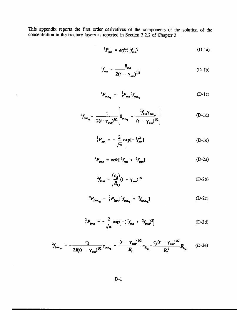
This appendix reports the first order derivatives of the components of the solution of theconcentration in the fracture layers as reported in Section 3.2.2 of Chapter 3.
p,,,,, = erfc( 1fin)
fM= - m
2(t - yu)1/2
Ilp . = l f
(D-la)
(D-lb)
(D-1c)
= 1 ' fmpYitn. 1'4116 2(t -_ yYn )+/2 (t- )1/2
1 2
P,, = _ 2 exi_ f,,^
2p = erfc[ If + 2f
2f = -t - 2
2i = 2 pb[lif + 2fi~m.
(D-ld)
(D-le)
(D-2a)
(D-2b)
(D-2c)
(D-2d)2 2
l~imn - eXp[-( ifI Pin = ~,/i.'
+ 2 2]
C2 = - A2R1(t - ysw; l/2
+ (t - yM") /2C
+ g &
C fl(t - y )12 2
RI2(D-2e)
D-1

3bpi = exp( 3f (D-3a)
3 _ e,,C,
3 Pm = 3pa 3fM,'v
(D-3b)
(D-3c)
3 f = Cfl eRia, -_
+ mftel.- Car
ftvD
4P M = ep[ 2t<,]
4Pmv = 2 4Pbm 2f 2f
spj~~exp[51Ij2]5P, = ex i]
Sf = ct
sPiv = 2 'P - t fi
(D-3d)
(D-4a)
(D-4b)
(D-5a)
(D-5b)
(D-5c)
I t 42
Al J� -&Cft tUnkR?
(D-5d)
(D-6a)
(D-6b)
6P = erfc(5fW
"Pi.. = "Pi I,
D-2

6pt = 2 e~p[5j~
7ps erfC( 7fp tgX
7fp,,= pA(t - yjl)2
7Api p iJP (far + TV.
7 f pu jlii(t-ysnm)1/2 G W +f
71P_=_ 2 ex_-(7ft + lf
8pjbx = exp[ 8fjb n
8X_ = to 2a + yj
up _ 8p U2 t - Pa
tf~hm. p 'ads + ads~., + 2 bPAP,(t-y.,, _ PJ~yIU
(D-6c)
(D-7a)
(D-7b)
(D-7c)
(D-7d)
(D-7e)
(D-8a)
(D-8b)
(D-8c)
(D-8d)
9 P = V3f (D-9a)
9p _ qf P& Pjfqf.--
As 2qj
(D-9b)
D-3

=P exp[ 'Ofh,] (D-lOa)
ly, = - ,Xn + 13i 2t (D-lOb)
op,= lopt lof (D-lOc)
°of = -,XX - aXX + 2I3SM13E, (D-lOd)
Ps= erfc(If if) (D-1la)
g1i= int 1/2 (D-llb)
pb. = lpi lfa (D-1lc)
Abe. = phwtW (D-1 Id)
1 = 2 PL a 4 2] (D-lle)
D-4

APPENDIX E
FIRST ORDER DERIVATIVES OF THE COMPONENTS OF THE CUMULATIVEMASS SOLUTION IN THE FRACTURE LAYERS

This appendix reports the first order derivatives of the cumulative mass in the fracture layers asreported in Section 3.2.3 of Chapter 3.
OG = e (E-1a)
OG = -OG t + 1AA (E-lb)
'G., = erf lh,,) (E-2a)
hm= (E-2b)2(t - y.)l
'Gm =' 1G,, hh (E-2c)
thmn, = 1+ _ (E-2d)' 2(t-yj1/2 (t - yJ-2
1 ~2IG,,= - exp[- 1hj (E-2e)
2GA = erfc[ h h ] (E-3a)
2h,, = V/(t - yJ (E-3b)
2G,. = 2G.*[ jh + 2 ] (E-3c)1 a Mk
2 = 2IG,; = - ex [-(lhm ± 2h)2 ] (E-3d)
E-1

2h I'a(t-Yn) - Ayen,.h21z. = -2(t-y,,,)] 12
3 Gt = 1 exp( h)
3h,,,, = - Axyt, + e3,,,,
- ! ±3 G,:n = 3G *43h,; - -
(E-3e)
(E-4a)
(E-4b)
(E-4c)
Oh,,c, X Ymn,,, - YM;La + emn'. �,x + PA ;2 V l)
(E-4d)
4Gt= ( * 1IA1Ru; )
(E-5a)
(E-5b)4 * = - 4G *2
'GLn = erfc[ ahr + Sh",] (E-6a)
5hi = CA fr - Y.),+
G& = -1Gi,.[ 1hm + SL,.
(E-6b)
(E-6c)
E-2

G= 2eXP[-(lh,, +5ho)2
5hiw,4g = - Cfl __ R _ _2RA(t -y." v A
(E-6d)
(E-6e)
- CI(t-y,)v2
k
lG,., = exp[6hi..]
The =-W + (-)(t - Y - t
6 G = 6Ghm 6hi,..
+-AtCx- C R)(t - y (Y A.
G = ((cO)
7= - 72 CA cR - AI}
'Gj&, = e*c( 'hj,,, + lh,,,,)
(E-7a)
(E-7b)
(E-7c)
(E-7d)
(E-8a)
(E-8b)
(E-9a)
E-3

OhJi = -(t - ym)l/ (E-9b)
SGp = 81Gj (8mn,, + )(E-9
8^X ̂ (t- Q - t - Y n (E-9d)
1 _ = - - eVp[ -( Shjb + l^)2] (E-9e)
9GobU= exp[ 9 h,,,, (E-lOa)
9hjin = 4u 2(t-y, - At (E-1Ob)
9Gjm%-w = 9Gjbm 9hjbm (E-lOc)
9hfl.% = ,U e. + pe,, + 2 P', P(t-y.) - y t- (E-lOd)
10Gfl = (E-lla)qua
1 G -= qP.i - P.Xqua (E-llb)q,
2
= N (P + 1) (E-12a)
E-4

JIGss= 2 FG;2 . (E-12b)
12Gi = exp[ 12hi] (E-13a)
12h = - anxn +Xpat - 1 t (E-13b)
12 G b = 12 Gt 12 h (E-13c)
2hot -aXx - CnX % + 2 tpbpb4 - t (E-13d)
13 G = erfc(1 3hn) (E-14a)
1h= pn t12 (E-14b)
13G = 13G 13h (E-14c)in~ I labs(E1)
1hi = p tIA (E-14d)
13 21 i21G = -- exp 1 - 13h 2] (E-14e)
4= 1 (E-15a)A
14G = -14G 2 (2PP - (E-15b)
E-5

l5G1 -= Cx (E-16a)
l5Gj, = ajX<) (E-16b)
6G. = 1 16 h (E-17a)
16 =(c i (At)2] (E-17b)16h = erf[(XLt)W~
16 P16i 12 ho J(E-17c)
16 Gj =16 h 16hb + lah h1, (E-17d)
= = jiexP-AIt)X (E-17e)
16 Pt. 1 3 ~
26^^w = aPt _ i Pin (E-17f)FI 2 13n 2
17G = e n 17h3 ) (E-18a)
7h = -( L t (E-18b)
E-6

1 2c71t(RlcJ - C-h e) - AE-18c)
17G =17GX 17h, (E-18d)
-G, erfc[ .h"] (E- 19a)
sh- CA ti (E-19b)
'$G,,.g = - 2 C(_ lg1h 2) jhh,, (-19c)
= (RIic,,. -cRf J 1)2 (E-19d)
RN
19G" = 16h l9h (E-20a)
l9h = CA (E-20b)
19G% = 16h6l9 h. + 16h '9h (E-20c)
where "16h is given by Equation (E-17b), and its derivative by Equation (E-17e)
-ICf" + 4 1) (E-20d)
N R,,2 Al~~h - -- L
E-7

APPENDIX F
NOTATIONS

ali, a2i, ai
Ai
AO
bi
b1i
Bi
Dei
Dd
Dpi
gf,
Ji
Kfi
K.j
Li
n
Q
R.
t
T
Tp
TI/2
constants in the model for residual concentrations in the ith fracture layer i
concentration of the species in the ith fracture layer
concentration of the species at the source at time equals to zero
half-thickness of the ith fracture layer
residual concentration in the ith rock matrix layer
concentration of the species in the ith rock matrix layer
effective diffusivity in the ith rock matrix layer
molecular diffusion of nuclide in water
pore diffusivity in the ith rock matrix layer
geometric factor of the ith rock matrix layer
diffusive rate of nuclide at surface of ith fracture layer per unit area of fracturesurface
surface distribution in the ith fracture layer
distribution coefficient in the ith rock matrix layer
thickness of ith rock matrix layer
total number of layers
steady water flow rate in fracture
retardation factor in the ith fracture layer
retardation factor in the ith rock matrix layer
time
leaching time
time period of a complete cycle (2 T/w)
half-life
F-1
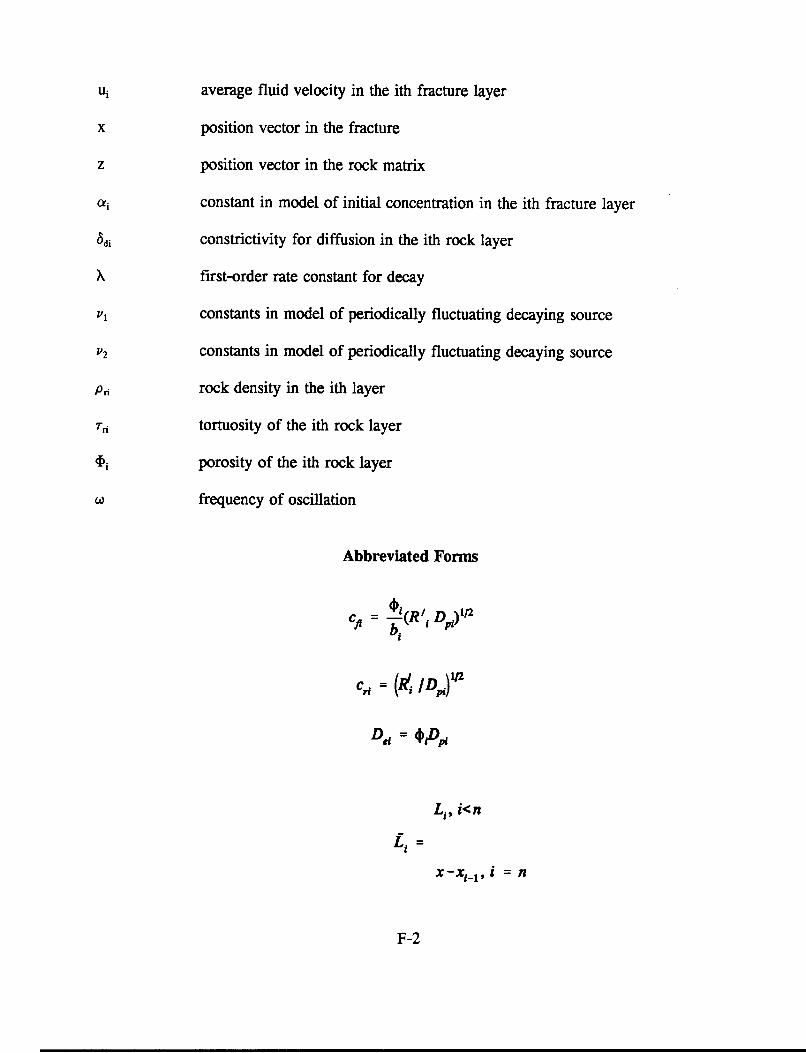
ui average fluid velocity in the ith fracture layer
x position vector in the fracture
z position vector in the rock matrix
a; constant in model of initial concentration in the ith fracture layer
adi constrictivity for diffusion in the ith rock layer
X first-order rate constant for decay
P I constants in model of periodically fluctuating decaying source
v2 constants in model of periodically fluctuating decaying source
PAi rock density in the ith layer
Tri tortuosity of the ith rock layer
(Di porosity of the ith rock layer
frequency of oscillation
Abbreviated Forms
cft = b (Rli Dpi)1/2
Drf = Rt Dp)D;= aPid
Li, i<n
Li =
x-ili =n
F-2
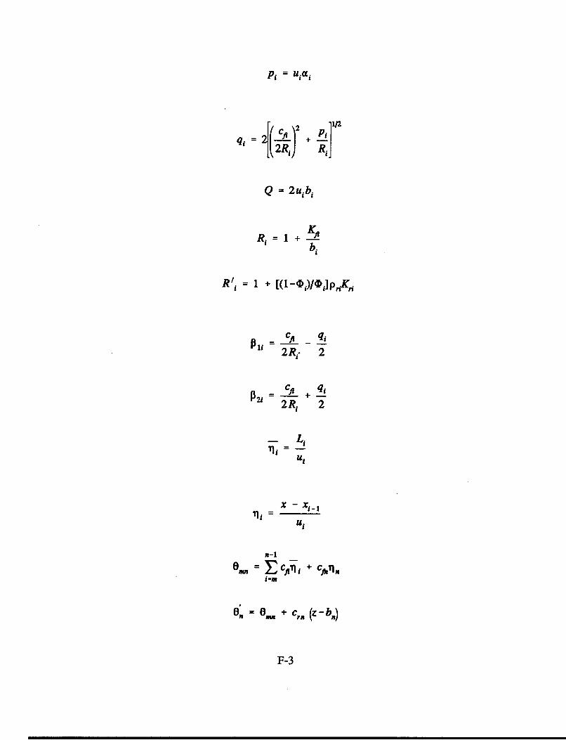
Pi = uiocc
q, + Pi~](2Rig Rij
Q = 2uibi
KR = 1 + +
bi
Rli =1 + [(1-4Di)lojiPnKA
li2RjP 2
P2i cR, 22Rj- 2
ui
x - XiC
U.
n-I
omnn Clfs i + C 1T,i-m
.n =f + crn (z-bn)
F-3

n-1
Y.m = ERjrli + Rni-m
x = x,
Xx-i
i = 1
ill
F-4

APPENDIX G
MODEL PARAMETERS

The following parameters are used in the computer code (written in ANSI StandardFORTRAN 77) that implements the analytic solutions described in Section 2.
FORTRAN NAME
ALFA(I)
CCO
CINF(1 ,I)
EXPLANATION
Constant alpha in the exponential term in residualconcentration mode in the ith fracture layer (1/L)
Concentration of the species at the source at time equalszero (units of activity/LI)
Constant in residual concentration model in the ith fracture(units of activity/lV)
CINF(2,I)
CINR(I)
CNS(1)
CNS(2)
DENSR(I)
Coefficient of exponential term in residual concentrationmodel in the ith fracture (units of activity/L3)
Residual concentration in the ith rock matrix layer (units ofactivity/L3)
Constant in periodically fluctuating decaying source termmodel (NPERIOD = 1)
Coefficient of sine function term in periodically fluctuatingdecaying source term model (NPERIOD = 1)
ith Rock matrix layer bulk density (M/L3) (used if IDIST(l)=2)
DIFFR(I) Pore diffusivity (L 2/T)
DIMENS(IJ) Dimensions used in the problem; each must be s 12characters in length.
(1,J) = Species name(2,J) = Time (year)(3,J) = Length (meter)(4,J) = L/T (meter/year)(5,J) = L2/T (m2/year)(6,J) = Mass/Volume (g/cc)(7,J) = Volume/Mass (cc/g)(8,J) = l/Time ( l./year)(9,J) = Units of Activity/Volume ( UA/L 3)(lO,J) = l/L (l./meter)
G-1

FORTRAN NAME
DISTX(I)
DISTRBF(I)
DISTRBR(I)
EXMAX
FLOWR
HALFL
HALF_THICK(I)
1AUTO
TIME
IBAND
ICONCF
ICONCR
ICUMF
IDIST(1)
EXPLANATION
Thickness of ith fracture or rock layer (L)
ith Fracture layer surface distribution coefficient (L)(IDIST(1) = 1)
ith Rock matrix layer distribution coefficient (L3IM)(IDIST(2) = 1)
Largest allowed magnitude for exponential arguments(machine dependent)
Steady water flow rate per unit width of fracture (L2/T)
Half-life of species (T)
Half-thickness of the ith fracture layer (L)
= 0 User supplies arrays REFX, REFZ, and TIMEincluding parameters NX, NZ and NT = 1 Automaticgeneration of arrays REFX, REFZ and
including parameters NX, NZ and NT (see Note)
= 0 Step release mode at source= 1 Band release mode at source
= 0 Do not calculate fracture concentrations= 1 Do calculate fracture concentrations
= 0 Do not calculate rock concentrations= 1 Do calculate rock concentrations
= 0 Do not calculate cumulative mass flux= 1 Do calculate cumulative mass flux
= 0 RETARDF corresponds to retardation factor infracture= 1 RETARDF corresponds to surface distributioncoefficient in fracture (i.e., DISTRBF)
G-2

FORTRAN NAME EXPLANATION
IDIST(2)
IGRAPH
= 0 RETARDR corresponds to retardation factor in rockmatrix= 1 RETARD R corresponds to distribution coefficient inrock matrix (i.e., DISTRBR)
= 0 Graphics output disabled= 1 Graphics output enabled; formatted graphics written tological unit 30, 31, 32, 35, 36
Logical Unit 30: Concentrations in Fractureof of 31: Concentrations in Rock Matrix
32: Cumulative Mass35: Concentration Sensitivities36: Cumulative Mass Sensitivities
INDEX(I) = 1 Evaluate sensitivity computation related to parameteri (i.e., NCONCSENSIT 22)= 0 Skip
Number of fracture/rock matrix layersLAYER
NCONCSENSIT = 1 Execute Module 1 (i.e., calculate concentrations andcumulative mass in the fractures and concentrations in therock matrix
= 2 Execute Module 2 (calculate sensitivity coefficients,relative sensitivies and variance
= 3 Execute both Modules 1 and 2
NPERIOD = 0 Continuously Decaying Source= 1 Periodically Fluctuating Decaying Source
NRUNMAX Number of data sets to be run
NT < 500, number of time values to be evaluated (skip ifIAUTO = 1)
NVAL Index for selecting solution module= 0 Option for analytical solutions= 1 Option for sensitivity module
G-3

FORTRAN NAME EXPLANATTON
NX < 500, number of positions to be evaluated in x direction(skip if IAUTO = 1)
NZ • 500, number of positions to be evaluated in x direction(skip if IAUTO = 1)
PERIOD Time period for a complete cycle of variation inperiodically fluctuating decaying source term model(NPERIOD = 1)
POROSR(I)
REFX(I)
REFZ(I)
RETARD F(I)
Average porosity in ith rock matrix layer
x-position in space (L) (read if IAUTO = 0)
z-position in space (L) (read if IAUTO = 0)
Retardation factor in the ith fracture layer (IDIST(l) = 0)or Surface distribution coefficient (i.e., DISTRB F) in theith fracture layer (IDIST(l) = 1)
RETARD R(I)
STDV(I)
TIME(I)
Retardation factor in the ith rock matrix layer (IDIST(2) =0) or Distribution coefficient (i.e., DISTRB_R) in the ithrock matrix layer(IDIST(2) = 1)
Standard deviation of parameter I (i.e., NCONCSENSIT2 2)
Position in time (T) (read if IAUTO = 0)
THML Leaching time A) (used if IBAND = 1)
TITLE 2 Lines, < 80 characters per line, title of data set
VELX(I) Average fluid velocity in the ith fracture layer (L/T)
Note: The following parameters are read-in if IAUTO = 1 in order to generate arrays REFX,REFZ and TIME and their associated parameters NX, NZ and NT.
X0 First value of spatial coordinate X = REFX(1)DX Spatial increment along X-axisENDX Final value of spatial coordinate X = REFX(NX)
G-4
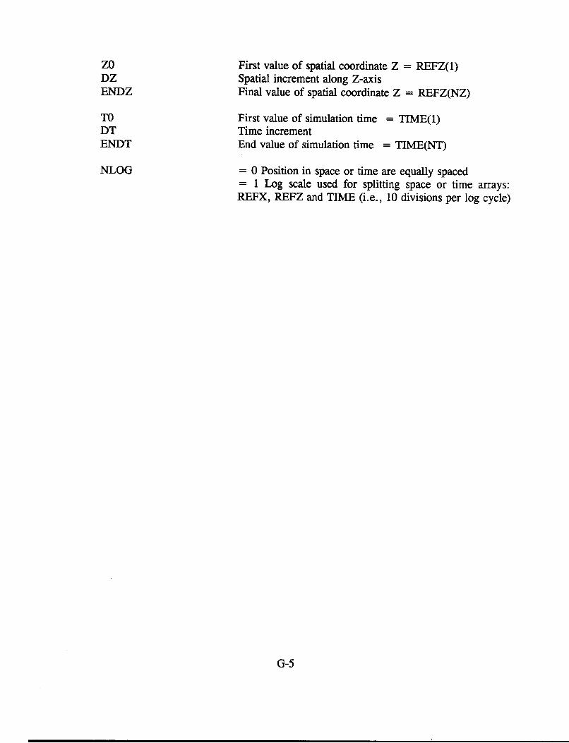
ZO First value of spatial coordinate Z = REFZ(1)DZ Spatial increment along Z-axisENDZ Final value of spatial coordinate Z = REFZ(NZ)
TO First value of simulation time = TIME(1)DT Time incrementENDT End value of simulation time = TIME(NT)
NLOG = 0 Position in space or time are equally spaced= 1 Log scale used for splitting space or time arrays:REFX, REFZ and TIME (i.e., 10 divisions per log cycle)
G-5


