Agronomic and Economic Comparison of Full-Season … committee members, Drs. David Holshouser, Wade...

Agronomic and Economic Comparison of Full-Season and Double-Cropped Small Grain and Soybean Systems in the Mid-Atlantic USA

by

Phillip W. Browning

Thesis submitted to the faculty of the Virginia Polytechnic Institute and State University in partial fulfillment of the requirements for the degree of

MASTER OF SCIENCE

In

Crop and Soil Environmental Sciences

David L. Holshouser, Chair

Wade E. Thomason, Co-Chair

Gordon E. Groover

Maria Balota

May 2, 2011 Blacksburg, Virginia

Keywords: Soybean, Cropping System, Planting Date, Profitability

Agronomic and Economic Comparison of Full-Season and Double-Cropped Small Grain and Soybean Systems in the Mid-Atlantic USA

Phillip W. Browning

ABSTRACT Increased demand for barley has changed the proportion of crops grown in Virginia and

the Mid-Atlantic USA. Winter wheat is the predominant small grain crop, but barley can be a

direct substitute, although much less of it is grown. Soybean is grown full-season and double-

cropped after both small grains. Historically, wheat was the primary small grain in the soybean

double-crop rotation because of its greater profitability. The barley-soybean cropping system is

not a new concept in the region, but the literature is outdated. New agronomic and economic

data that directly compares full-season soybean, barley-soybean, and wheat-soybean systems

using modern cultivars and management practices is needed. The objectives of this research

were to: i) determine soybean yield and compare cropping system profitability of the three

cropping systems; ii) perform a breakeven sensitivity analysis of the three cropping systems; and

iii) determine the effect of planting date and previous winter crop on soybean yield and yield

components. Soybean grown after barley yielded more than full-season soybean in two of six

locations and more than soybean double-cropped after wheat in three of six locations. Net

returns for the barley-soybean system were the greatest. These data indicate that soybean

double-cropped after barley has the potential to yield equal to or greater than full-season soybean

or double-cropped soybean following wheat, but its relative yield is very dependent on growing

conditions. The profitability comparison indicated that the barley-soybean cropping system was

generally more profitable than the full-season soybean and double-cropped wheat-soybean

systems. This conclusion was supported by the breakeven sensitivity analysis, but remains

dependent on prices that have been extremely volatile in recent years. In another study, soybean

iii

yields declined with planting date at two of four locations in 2009, a year that late-season rainfall

enabled later-planted soybean to yield more than expected. In 2010, soybean yield decline was

affected by the delay in planting date at both locations. Winter grain did not affect soybean yield

in either year. Yield component data reinforced these results and indicated that the lower seed

yield in the later planting dates was due primarily to a decrease in the number of pods.

iv

Acknowledgements

I would like to thank Osage Bio Energy, the Virginia Soybean Board, and the Virginia

Small Grains Board, whose funding has made this research possible. I would also like to thank

my committee members, Drs. David Holshouser, Wade Thomason, Gordon Groover, and Maria

Balota, for the unique knowledge and advice they have each shared with me during this project.

I am very grateful to all of the faculty and staff at Tidewater AREC for the encouragement they

have given me. I would like to especially thank the soybean team, Patsy Lewis, Mike Ellis, Ed

Seymore, and Amro Ahmed for their invaluable help, patience, and sense of humor during the

long hours over these past two years. Without them this project would not have been possible.

Sine quibus non.

v

Table of Contents

Abstract ........................................................................................................................................... ii

Acknowledgements ........................................................................................................................ iv

Table of Contents ............................................................................................................................ v

List of Tables ................................................................................................................................. vii

List of Figures ................................................................................................................................ ix

Chapter 1. Introduction and Justification ....................................................................................... 1

References ........................................................................................................................... 5

Chapter 2. Yield and Profitability Comparisons of Full-Season Soybean, Double-Cropped

Wheat-Soybean, and Double-Cropped Barley-Soybean Systems

Abstract ............................................................................................................................. 10

Introduction ....................................................................................................................... 12

Materials and Methods ...................................................................................................... 13

Results and Discussion ...................................................................................................... 17

References ......................................................................................................................... 25

Chapter 3. Breakeven Sensitivity Analysis of Full-Season and Double-Cropped Soybean

Systems

Introduction ....................................................................................................................... 36

Example Calculation ......................................................................................................... 39

Explanation of the Excel Model ........................................................................................ 41

Interpretations.................................................................................................................... 48

Profitability Scenarios ....................................................................................................... 50

References ......................................................................................................................... 53

vi

Chapter 4. Soybean Planting Date and Small Grain Residue Effects on Soybean Yield and Yield

Components

Abstract ............................................................................................................................. 54

Introduction ....................................................................................................................... 55

Materials and Methods ...................................................................................................... 57

Results and Discussion ...................................................................................................... 60

References ......................................................................................................................... 66

Appendix A: Production costs used to calculate net returns for full-season and double-cropped

soybean systems from 2008-2010. .................................................................................... 95

Appendix B: Annual, average, and median prices for soybean, barley, wheat, and corn across

Virginia and at several delivery stations from 2006 to 2010 ............................................ 97

Appendix C: Full-season, double-cropped barley-soybean, and double-cropped wheat-soybean

example enterprise budgets ............................................................................................. 100

vii

List of Tables

Chapter 1.

Table 1.1 – Hectarage comparisons of small grain and soybean in Virginia and the Mid-Atlantic

..............................................................................................................................................9

Chapter 2.

Table 2.1 – Soil series and yield potential for 2009 and 2010 experimental locations ................. 28

Table 2.2 – Locations and small grain cultivars used at various planting dates for the 2008-2009

and 2009-2010 growing seasons ....................................................................................... 29

Table 2.3 – Locations, soybean cultivars, and planting dates for full-season and double-crop

systems in 2009 and 2010 ................................................................................................. 30

Table 2.4 – Analysis of variance for small grain and soybean yields in full-season and double-

crop systems in 2009 and 2010 ......................................................................................... 30

Table 2.5 – Barley, wheat, and soybean yields in four cropping systems in 2009 and 2010 ........ 31

Table 2.6 – Analysis of variance for barley, wheat, and soybean net returns in full-season and

double-crop systems in 2009 and 2010 ............................................................................. 32

Table 2.7 – Net returns above production costs in four cropping systems in 2009 and 2010 ...... 33

Chapter 3.

Table 3.1 – Five-year soybean, barley, and wheat prices at various percentiles .......................... 50

Table 3.2 – Full-season soybean, double-cropped barley-soybean, and double-cropped wheat-

soybean system profitability at various yields and prices ................................................. 51

Chapter 4.

Table 4.1 – Soil series and yield potential for 2009 and 2010 experimental locations ................. 68

Table 4.2 – Locations and soybean cultivars used at various planting dates in 2009 ................... 69

viii

Table 4.3 – Locations and soybean cultivars used at various planting dates in 2010 ................... 69

Table 4.4 – Treatment effects for soybean yield component measurements at four locations in

2009 ................................................................................................................................... 70

Table 4.5 – Treatment effects for soybean yield component measurements at two locations in

2010 ................................................................................................................................... 71

Table 4.6 – Seed yield, plant biomass, height, and yield components of soybean planted on

different dates into a rye cover crop, or into barley or wheat harvested for grain at

EVAREC in 2009 .............................................................................................................. 72



SPAREC in 2009 ............................................................................................................... 74



TAREC1 in 2009 ............................................................................................................... 76



TAREC2 in 2009 ............................................................................................................... 78


different dates into rye, barley, wheat, or previous crop residue at TAREC3 in 2010 ..... 80


different dates into rye, barley, wheat, or previous crop residue at TAREC4 in 2010 ..... 85

ix

List of Figures

Chapter 2.

Fig. 2.1 – Maximum and minimum temperatures and rainfall at EVAREC, SPAREC, and

TAREC in 2009, and TAREC in 2010 .............................................................................. 34

Chapter 3.

Fig. 3.1 – Wheat vs. Barley Breakeven Prices .............................................................................. 48

Fig. 3.2 – Wheat vs. Full-Season Soybean Breakeven Prices ....................................................... 49

Fig. 3.3 – Barley vs. Full-Season Soybean Breakeven Prices....................................................... 49

Chapter 4.

Fig. 4.1 – Influence of planting date and winter grain on full-season and double-cropped soybean

yield at EVAREC, SPAREC, TAREC1, and TAREC2 in 2009 ....................................... 90

Fig. 4.2 – Influence of planting date on full-season and double-cropped soybean yield at

TAREC3 and TAREC4 in 2010 ........................................................................................ 92

Fig. 4.3 – Maximum and minimum temperatures and rainfall at EVAREC, SPAREC, and

TAREC in 2009, and TAREC in 2010 .............................................................................. 93

1

Chapter 1 – Introduction and Justification

Appomattox Bio Energy, owned by Osage Bio Energy, built a barley-based ethanol plant

in eastern Virginia, near Hopewell. The company purchases barley (Hordeum vulgare L.) grown

regionally for use at this plant. Anecdotal evidence suggests barley hectarage has increased due

to the ethanol plant, substituting for land allocated for wheat (Triticum aestivum L.) or replacing

land allocated for full-season soybean [Glycine max (L.) Merr.]. Winter wheat is the

predominant small grain crop grown in the Mid-Atlantic USA (, Delaware, Maryland, New

Jersey, North Carolina, and Pennsylvania, Virginia). Barley can be a direct substitute for wheat,

but much less of it is grown. Soybean is grown full-season (May-planted) and double-cropped

after both small grains (Table 1.1) (National Agricultural Statistics Service, 2011). The

Commonwealth of Virginia follows similar trends, with much more wheat grown than barley,

but grows proportionally more double-cropped soybean than the rest of the Mid-Atlantic.

Historically, wheat was the primary small grain in the soybean double-crop rotation because of

its greater profitability. That is, net returns over costs were greater for the wheat-soybean

rotation than for the barley-soybean rotation. Little current information is available comparing

the profitability of barley-soybean, wheat-soybean, and full-season soybean cropping systems.

The literature is replete with evidence that wheat-soybean double-cropped systems can

generate higher net returns than full-season soybean (Crabtree and Rupp, 1980; Farno et al.,

2002; Kelley, 2003; Kyei-Boahen and Zhang, 2006; Sanford, 1982; Sanford et al., 1986; Wesley,

1999; Wesley and Cooke, 1988; Wesley et al., 1994, Wesley et al., 1991; Wesley et al., 1995).

There are fewer reports of the opposite. In certain situations, irrigated full-season soybean

brought greater returns than non-irrigated double-cropped soybean in the mid-South (Wesley and

2

Cooke, 1988; Wesley et al., 1994; Wesley et al., 1995). In higher latitudes with shorter growing

seasons, full-season systems provided greater returns than double-cropped systems (Moomaw

and Powell, 1990). These scenarios should be reanalyzed using updated prices and input costs.

Other double-crop systems aside from wheat-soybean have been studied as well. In

Oklahoma and Iowa, sorghum [Sorghum bicolor (L.) Moench] was successfully double-cropped

after wheat and triticale, respectively (Crabtree et al., 1990, Goff et al., 2010). In Mississippi,

grain sorghum as well as sunflower (Helianthus annuus L.) planted after wheat was successfully

grown, but were not as profitable as wheat-soybean in an irrigated environment (Sanford et al.,

1973; Sanford et al., 1986, Wesley et al., 1994). In a non-irrigated environment, a rotation that

included grain sorghum had returns greater than $60 ha-1 more than traditional cropping systems

(Wesley et al., 1995).

Less research is available regarding double-cropping soybean with barley. Double-crop

soybean has been successful when harvested after barley and oats (Avena sativa L.) grown as

spring forage in the upper Midwest (Kaplan and Brinkman, 1984; LeMahieu and Brinkman,

1990). Research conducted from 1972 to 1975 in Kentucky found that soybean following barley

yielded similarly to full-season soybean (Herbek and Bitzer, 1998). In Virginia, soybean, grain

sorghum, and corn (Zea mays L.) were all profitable when double-cropped after barley harvested

for grain (Camper et al., 1972). Groover et al. (1989) concluded that a grain farm in eastern

Virginia should include a barley-soybean rotation to maximize income at varying levels of risk.

However, these conclusions need to be reanalyzed using today’s prices and input costs.

While a wheat-soybean double-crop system may generate more net returns than full-

season soybean, the seed yield of full-season soybean is typically greater relative to the soybean

double-cropped after wheat (Caviness and Collins, 1985; Kelley, 2003; Kyei-Boahen and Zhang,

3

2006; Sanford et al., 1986; Wesley, 1999; Wesley and Cooke, 1988; Wesley et al., 1988; Wesley

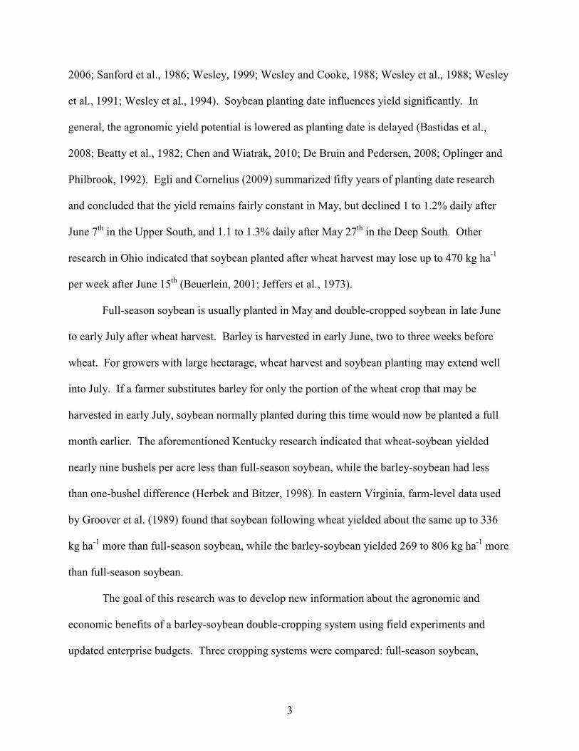
et al., 1991; Wesley et al., 1994). Soybean planting date influences yield significantly. In

general, the agronomic yield potential is lowered as planting date is delayed (Bastidas et al.,

2008; Beatty et al., 1982; Chen and Wiatrak, 2010; De Bruin and Pedersen, 2008; Oplinger and

Philbrook, 1992). Egli and Cornelius (2009) summarized fifty years of planting date research

and concluded that the yield remains fairly constant in May, but declined 1 to 1.2% daily after

June 7th in the Upper South, and 1.1 to 1.3% daily after May 27th in the Deep South. Other

research in Ohio indicated that soybean planted after wheat harvest may lose up to 470 kg ha-1

per week after June 15th (Beuerlein, 2001; Jeffers et al., 1973).

Full-season soybean is usually planted in May and double-cropped soybean in late June

to early July after wheat harvest. Barley is harvested in early June, two to three weeks before

wheat. For growers with large hectarage, wheat harvest and soybean planting may extend well

into July. If a farmer substitutes barley for only the portion of the wheat crop that may be

harvested in early July, soybean normally planted during this time would now be planted a full

month earlier. The aforementioned Kentucky research indicated that wheat-soybean yielded

nearly nine bushels per acre less than full-season soybean, while the barley-soybean had less

than one-bushel difference (Herbek and Bitzer, 1998). In eastern Virginia, farm-level data used

by Groover et al. (1989) found that soybean following wheat yielded about the same up to 336

kg ha-1 more than full-season soybean, while the barley-soybean yielded 269 to 806 kg ha-1 more

than full-season soybean.

The goal of this research was to develop new information about the agronomic and

economic benefits of a barley-soybean double-cropping system using field experiments and

updated enterprise budgets. Three cropping systems were compared: full-season soybean,

4

double-cropped wheat-soybean, and double-cropped barley-soybean. The objectives of this

study were to:

(1) Determine soybean yield and compare cropping system profitability of the three cropping

systems.

(2) Perform a breakeven sensitivity analysis of the three cropping systems.

(3) Determine the effect of planting date and previous winter crop on soybean yield and yield

components.

5

REFERENCES

Bastidas, A.M., Setiyono, T.D., Dobermann, A., Cassman, K.G., Elmore, R.W., Graef, G.L.,

and Specht, J.E. Soybean sowing date: the vegetative, reproductive, and agronomic

impacts. 2008 Crop Sci. 48:727-740.

Beatty, K.D., Eldridge, I.L., and Simpson, A.M., Jr. 1982. Soybean response to different

planting patterns and dates. Agron. J. 74: 559-562.

Beuerlein, J. 2001. Doublecropping soybeans following wheat. Ohio State University

Extension. AGF-103-01.

Camper, H.M., Jr., Genter, C.F., and Loope, K.E. 1972. Double cropping following winter

barley harvest in eastern Virginia. Agron. J. 64:1-3.

Caviness, C.E., and F.C. Collins. 1985. Double cropping. In Shibles, R.M. (ed.) World

Soybean Research Conference III. Westview Press. Boulder and London.

Chen, G., and Wiatrak, P. 2010. Soybean development and yield are influenced by planting

date and environmental conditions in the southeastern coastal plain, United States. Agron.

J. 102: 1731-1737.

Crabtree, R.J. and Rupp, R.N. 1980. Double and monocropped wheat and soybeans under

different tillage and row spacings. 72:445-448.

Crabtree, R.J., Prater, J.D., and Mbolda, P. 1990. Long-term wheat, soybean, and grain

sorghum doublecropping under rainfed conditions. Agron. J. 82:683-686.

De Bruin, J.L., and Pedersen, Palle. 2008. Soybean seed yield response to planting date and

seeding rate in the upper Midwest. Agron. J. 100:696-703.

Egli, D.B., and Cornelius, P.L. 2009. A regional analysis of the response of soybean yield to

planting date. Agron. J. 101: 330-335.

6

Farno, Luke A., Edwards, Lewis H., Keim, K., and Epplin, F.M. 2002. Economic analysis of

soybean-wheat cropping systems. Online. Crop Management doi: 10.1094/CM-2002-

0816-01-RS.

Goff, B.M., Moore, K.J., Fales, S.L., and Heaton, E.A. 2010. Double-Cropping Sorghum for

Biomass. Agron. J. 102:1586-1592.

Groover, G.E., Kenyon, D.E., and Kramer, R.A. 1989. An evaluation of production and

marketing strategies for eastern Virginia cash grain producers. Ext. Pub. 89-1. VA Coop.

Ext., Virginia Tech, Blacksburg.

Herbek, J.H., and M.J. Bitzer. 1998. Soybean production in Kentucky part III: planting

practices and double cropping. Ext. Pub. AGR-130. KY Coop. Ext. Svc, University of

Kentucky. http://www.ca.uky.edu/agc/pubs/agr/agr130/agr130.htm [Accessed 23

February 2011].

Jeffers, D.L., and Triplett, G.B., and Beuerlein, J.E. 1973. Management is the key to success:

double-cropped soybeans after wheat. Ohio Report on Research and Development. 58:67-

69.

Kaplan, S.L., and Brinkman, M.A. 1984. Multiple cropping soybean with oats and barley.

Agron. J. 76:851-854.

Kelley, K.W. 2003. Double-cropping winter wheat and soybean improves net returns in the

eastern Great Plains. Online. Crop Management doi: 10.1094/CM-2003-1112-01-RS.

Kyei-Boahen, S., and Zhang, L. 2006. Early-maturing soybean in a wheat- soybean double-crop

system: yield and net returns. Agron. J. 98:295-301.

LeMahieu, P.J., and Brinkman, M.A. 1990. Double-cropping soybean after harvesting small

grains as forage in the north central USA. J. Prod. Agric. 3:385-389.

7

Moomaw, R.S., and Powell, T.A. 1990. Multiple cropping systems in small grains in northeast

Nebraska. J. Prod. Agric. 3:569-576.

National Agricultural Statistics Service. 2011. U.S. & All States Data – Crops [Online].

Available at http://www.nass.usda.gov/QuickStats/Create_ Federal_All.jsp [accessed 10

February 2011].

Oplinger, E.S., and Philbrook, B.D. 1992. Soybean planting date, row width, and seeding rate

response in three tillage systems. J. Prod. Agric. 5:94-99.

Sanford, J.O., Myhre, D.L., and Merwine, N.C. 1973. Double cropping systems involving no-

tillage and conventional tillage. Agron J. 65:978-982.

Sanford, J.O. 1982. Straw and Tillage Practices in Soybean-Wheat Double-Cropping. Agron. J.

74:1032-1035.

Sanford, J.O., Eddleman, B.R., Spurlock. S.R., and J.E. Hairston. 1986. Evaluating ten cropping

alternatives for the midsouth. Agron. J. 78:875-880.

Wesley, R.A., and Cooke, F.T. 1988. Wheat-soybean double-crop systems on clay soil in the

Mississippi Valley area. J. Prod. Agric. 1:166-171.

Wesley, R.A., Heatherly, L.G., Elmore, C.D. and Spurlock, S.R. 1994. Net returns from eight

irrigated cropping systems on clay soil. J. Prod. Agric. 7:109-115.

Wesley, R.A., Heatherly, L.G., and Elmore, C.D. 1991. Cropping systems for clay soil: crop

rotation and irrigation effects on soybean and wheat doublecropping. J. Prod. Agric.

4:345-352.

Wesley, R.A., Heatherly, L.G., Elmore, C.D., and Spurlock, S.R. 1995. Net returns from eight

nonirrigated cropping systems on clay soil. J. Prod. Agric. 8: 514-520.

8

Wesley, R.A., Heatherly, L.G., Pringle, H.C., III, and Tupper, G.R. 1988. Seedbed tillage and

irrigation effects on yield of mono- and doublecrop soybean and wheat on a silt loam.

Agron. J. 80:139-143.

9

Table 1.1. Hectarage comparisons† of small grain and soybean in Virginia and the Mid-Atlantic‡.

Virginia

Mid-Atlantic

Crop

2009

2010

2009

2010

Planted all purposes (1,000 ha)

Barley

27

30

94

89

Wheat

101

73

597

447

Soybean

235

227

1453

1368

† SOURCE: National Agricultural Statistics Service, 2011. ‡ Mid-Atlantic states include: Delaware, Maryland, New Jersey, North Carolina, Pennsylvania, and Virginia.

10

Chapter 2 – Yield and Profitability Comparisons of Full-Season Soybean, Double-Cropped

Wheat-Soybean, and Double-Cropped Barley-Soybean Systems

ABSTRACT

Full-season soybean and double-cropped soybean [Glycine max (L.) Merr.] after wheat

(Triticum aestivum L.) are the predominant soybean cropping systems in the Mid-Atlantic USA.

Double-cropping soybean after barley (Hordeum vulgare L.) presents an additional option, but

new agronomic and economic data directly comparing barley-soybean with wheat-soybean and

full-season soybean systems using updated prices, costs, and management practices are needed.

Field studies were conducted to compare yield and net returns from a double-cropped barley-

soybean system with double-cropped wheat-soybean and full-season soybean systems. Soybean

grown after barley yielded 629 and 1458 kg ha-1 more than full-season soybean grown after a rye

cover crop in two of six locations and 462, 680, and 955 kg ha-1 more than soybean double-

cropped after wheat in three of six locations. Wheat yields ranged from 1448 to 4463 kg ha-1

across all locations and years, and contributed 37-56% of the total gross returns for the double-

cropped wheat-soybean system. Barley yields ranged from 3820 to 6766 kg ha-1 across all

locations and years, and contributed 30-52% or 26-47% of the total gross returns for the double-

cropped barley-soybean system, depending on the barley price estimation method. Two barley

pricing strategies were used in the profitability comparison. Using the first strategy, net returns

for the barley-soybean system were greater than full-season soybean at three of four locations in

2009, averaging $234 to 620 ha-1, and greater than double-cropped wheat-soybean at three of

four locations, averaging $234 to 506 ha-1. The barley-soybean cropping system at the second

barley pricing strategy had net returns greater than the full-season soybean grown after rye at

11

every location, averaging $95 to 757 ha-1, and greater than the double-cropped wheat-soybean

system in three of four locations, averaging $364 to 634 ha-1. In 2010, the double-cropped

barley-soybean system net returns using the first barley pricing strategy were not different from

the full-season soybean or double-cropped wheat-soybean systems averaged across locations. At

the second barley pricing strategy, the double-cropped barley-soybean system net returns were

$108 and 130 ha-1 greater than the full-season rye-soybean and double-cropped wheat-soybean

systems, respectively. These data indicate that soybean double-cropped after barley has the

potential to yield equal to or greater than full-season soybean or double-cropped soybean

following wheat, but performance is dependent on rainfall amount and distribution. The

profitability analysis indicated that the barley-soybean cropping system could be more profitable

than either the full-season soybean or double-cropped wheat-soybean systems.

12

INTRODUCTION

Full-season and double-cropped small grain-soybean are common soybean cropping

systems in the Mid-Atlantic USA (National Agricultural Statistics Service, 2011). Full-season

soybean is usually planted in May and is the only crop grown during that calendar year. The

wheat-soybean double-cropping system includes planting winter wheat in October through

November, harvesting that crop at the end of June, and planting soybean immediately following

wheat harvest. A barley-soybean double-cropping system includes planting barley in October,

followed by barley harvest and soybean planting in early June. Barley harvest occurs two to

three weeks before wheat. The longer soybean growing season after barley has the potential to

increase soybean yield and system profitability.

It is well documented that full-season soybean yields more than double-cropped soybean

after wheat (LeMahieu and Brinkman, 1990; Sanford et al., 1986; Wesley et al., 1994; Wesley et

al., 1995). At the same time, the double-crop wheat-soybean rotation as a whole is more

profitable than full-season soybean alone, shown most recently in Kansas (Kelley, 2003) and

Mississippi (Kyei-Boahen and Zhang, 2006; Wesley, 1999). Little research has been conducted

with soybean grown after barley.

LeMahieu and Brinkman (1990) conducted a study where full-season soybean was

compared with several double-crop soybean rotations grown after small grain in the Upper

Midwest, including winter wheat and spring barley grown as forage crops. Full-season soybean

had the greatest yield, but the double-cropped barley-soybean and wheat-soybean rotations were

more profitable. The wheat-soybean double-cropped system was more profitable than the

barley-soybean double-cropped system, but soybean following barley yielded equally to soybean

following wheat. In a 1972-75 research project conducted in Kentucky, Herbek and Bitzer

13

(1998) found that soybean grown after barley did not yield significantly less than full-season

soybean. Double-cropped wheat-soybean was not included in that study. In Virginia, Camper et

al. (1972) found that a barley-soybean double-crop system was viable and profitable, but it was

not compared to either full-season soybean or double-crop wheat-soybean. Groover et al. (1989)

compared the risk of several crop rotations, and concluded that an eastern Virginia grain farm

should include a double-crop barley-soybean rotation. This 1989 Virginia study used historical

yield records, but did not include any yield trials. New agronomic and economic data directly

comparing barley-soybean with wheat-soybean and full-season soybean systems are needed.

We hypothesize soybean double-cropped after barley yields less than full-season soybean

but greater than soybean double-cropped after wheat, and that a barley-soybean cropping system

can be more profitable than either full-season soybean or double-cropped wheat-soybean,

depending on yields and prices. We assumed that barley planted in October would be harvested

two to three weeks earlier than wheat planted in November, thereby lengthening the double-crop

soybean growing season and providing for greater soybean yield, which would contribute to the

total system profitability. The objectives of this study were to (i) compare the yields of double-

crop barley-soybean with yields of full-season soybean and double-crop wheat-soybean, and (ii)

compare the net returns from all the cropping systems.

MATERIALS AND METHODS Experiments were conducted from fall 2008 through fall 2009 at the Eastern Virginia

Agricultural Research and Extension Center (EVAREC) near Warsaw on a Kempsville loam

(fine-loamy, siliceous, subactive, thermic typic hapludults), the Southern Piedmont Agricultural

Research and Extension Center (SPAREC) near Blackstone on an Appling fine sandy loam (fine,

14

kaolinitic, thermic typic kanhapludults), and two sites at the Tidewater Agricultural Research and

Extension Center (TAREC1 and TAREC2) near Suffolk, Virginia. A Eunola loamy fine sand

(fine-loamy, siliceous, semiactive, thermic aquic hapludults) and a Rains fine sandy loam (fine-

loamy, siliceous, semiactive, thermic, typic paleaquults) (tile-drained) represented the soils at

TAREC1 and TAREC2, respectively. Experiments were repeated from fall 2009 through fall

2010, but drought and poor emergence and growth during the 2010 growing season prevented

accurate data collection at EVAREC and SPAREC. A Nansemond loamy fine sand (coarse-

loamy, siliceous, subactive, thermic aquic hapludults) and a Dragston fine sandy loam (coarse-

loamy, mixed, semiactive, thermic aeric endoaquults) (tile-drained) represented the soils at

TAREC3 and TAREC4, respectively. The soil yield potentials for all sites are shown in Table

2.1.

Experimental design for both growing seasons was a randomized complete block with

four replications. In 2008-2009, plots were the small grain crops rye (as a cover crop), barley,

and wheat (Table 2.2). Soybean was grown full-season after killed rye and double-cropped after

harvested barley and wheat. In 2009-2010, plots were the same, but an additional full-season

fallow-soybean plot was added due to grower interest. The initial planting dates for full-season

soybean were in May, while the initial planting dates for double-cropped soybean followed small

grain harvest (Table 2.3).

The barley and wheat cultivars at all locations were Thoroughbred (Virginia Crop

Improvement Association, Richmond, VA) and SS520 (Southern States Cooperative, Richmond,

VA), respectively. Thoroughbred is a late-maturing winter barley cultivar, while SS520 is an

early-maturing, soft red winter wheat cultivar. Although SS520 yields less than later-maturing

wheat cultivars, it was used so that soybean following wheat could be planted as early as

15

possible, a practice that Virginia farmers follow to minimize the effect of late planting date.

Soybean cultivars and planting dates are shown in Table 2.3. Soybean cultivar 95Y70 (Pioneer

Hi-Bred, Int’l, Johnson, IA) is a maturity group V and contains resistance to root knot nematode

(Melooidogyne spp.), which was known to be present in low numbers at TAREC1 in 2009.

AG4907 (Monsanto Co., St. Louis, MO) is a maturity group IV cultivar, and was used to

facilitate earlier harvest on TAREC2 and TAREC4, fields that can become wet during November

and inhibit timely harvest. Otherwise, AG4907 and AG5605 are both considered standard high-

yielding cultivars at their respective locations.

Fields were fertilized with phosphate and potash according to soil tests. Nitrogen needs

for small grains varied and were met with 25-35 kg ha-1 at planting followed by split applications

based on tiller counts and tissue analysis (Alley et al., 2009a; Alley et al., 2009b). Soybean was

no-till planted within three days of small grain harvest using a five-row plot planter in 2009 and

a thirteen-row drill in 2010. Row spacing was 38 and 19 cm for the planter and drill,

respectively. Soybean seeding rates gradually increased with planting date, based on the

standard guidelines recommended by Virginia Cooperative Extension (Holshouser, 2010). In

2009, individual plots were 7.3 m long by 4.6, 5.5, 3.6, and 3.6 m wide at EVAREC, SPAREC,

TAREC1, and TAREC2, respectively. In 2010, individual plots were 7.3 m long by 4.9 m wide.

The land was disked and land-conditioned before small grain planting and soybean was planted

no-till. In 2009, TAREC2 received 1.4 and 0.67 kg ha-1 of manganese and sulfur, respectively,

in mid-July to correct visual manganese deficiency. In 2010, TAREC3 and TAREC4 received

0.13 and .054 kg ha-1 of manganese and sulfur, respectively, in mid-July. Standard pesticides

were applied to control weeds, insects, and diseases for all crops, per Virginia Cooperative

Extension recommendations (Herbert and Hagood, 2011). TAREC1 was irrigated once in 2009

16

(15 July) with 50 mm and TAREC3 was irrigated twice in 2010 (1 and 20 July), with 25 mm on

each occasion. Small grain and soybean were harvested with a plot combine equipped with a

weigh bucket and moisture sensor. Yields were adjusted to 130 g kg-1 moisture content.

Profitability was calculated to determine the net returns over variable and fixed

production costs for all cropping systems using the Virginia Enterprise Budget System Generator

(Eberly, 2010). Variable costs included seed, fertilizer, pesticides, applications, equipment

maintenance and repair, labor, crop insurance, operating loan interest, and hauling; fixed costs

included general overhead and yearly equipment ownership costs (Appendix A). Total costs did

not include storage, drying, scouting, or land costs. Five-year average (2006-2010) Virginia

commodity prices were used for soybean, barley, and wheat in the budgets (National

Agricultural Statistics Service, 2011). An additional barley price was calculated as 80% of five-

year average Chicago Mercantile Exchange July corn future prices for January 2006-December

2010 (FutureSource, 2011). The second barley price was based on the pricing mechanism of

Osage Bio Energy, a relatively new company that is purchasing barley for ethanol production in

eastern Virginia. Prices used to calculate gross income were $0.354, $0.176, $0.122, and $0.153

kg -1 for soybean, wheat, barley (Virginia price), and barley (Osage price), respectively

(Appendix B). Gross income was calculated by multiplying yield by the five-year average price.

Net returns over total costs were calculated by subtracting total costs from the gross income.

Yield and net returns were subjected to analysis of variance using PROC GLM (SAS

Institute, 2008). Years were analyzed separately because of the additional full-season fallow-

soybean plots in 2010. Location and cropping system were considered fixed factors, while

blocks were considered random. Least square means of the fixed effects were calculated and

separated using the PDIFF statement at P = 0.05.

17

RESULTS AND DISCUSSION

Yield Comparison

In 2009, only brief periods without rainfall were experienced and precipitation generally

increased as the season progressed, resulting in better than average growth for the double-crop

soybean systems (Fig. 2.1). In 2010, soybean experienced one of the hottest and driest growing

seasons of the last century. TAREC3 was irrigated (25 mm) twice during the worst of the

drought. These were emergency irrigations to salvage the experiment, without which there may

have been no appreciable soybean yield. TAREC4 could not be irrigated, but the Dragston soil

at this site had greater water holding capacity. At TAREC, rainfall during the summer months of

June, July, and August totaled 295 mm in 2009 compared to 99 mm in 2010. Temperatures were

also much hotter in 2010 than 2009, frequently reaching or exceeding 40°C. At the end of the

2010 growing season, soybean plots received 324 mm of rainfall in one week from the end of

September to the start of October.

There were cropping system and location differences and a cropping system by location

interaction for small grain yield in 2009 (Table 2.4). In 2010, cropping system and location

differences remained, but there was no interaction. Barley yielded more than wheat at all

locations except for TAREC1 and TAREC2 (Table 2.5). Barley yields ranged from 3820 to

6766 kg ha-1 across all locations and years (Table 2.5). This is generally in keeping with

Virginia’s 2006-2010 average yield of 4021 kg ha-1, although in all cases except EVAREC yields

were below the corresponding soil yield potential (Table 2.1) (National Agricultural Statistics

Service, 2011). Wheat yields ranged from 1448 to 4463 kg ha-1 across all locations and years

(Table 2.5). All but two locations were less than Virginia’s 2006-2010 average yield of 4193 kg

ha-1 (National Agricultural Statistics Service, 2011). At all locations the yields were less than the

18

soil yield potential (Table 2.1). Wheat at SPAREC yielded far below anticipated yield, but could

be attributed to very poor stands. Other yield differences could be due to variations in rainfall

and/or soil types between the different locations.

In 2009, barley was harvested during the first week of June at all TAREC locations and

the second week of June at EVAREC and SPAREC. Wheat at TAREC1 and TAREC2 matured

during the first and second weeks of June, respectively, which is unusually early, due to warm

and dry weather. Wheat was harvested during the fourth week of June at EVAREC and

SPAREC. In 2010, barley was harvested during the first week of June at TAREC3 and

TAREC4. Wheat matured in mid-June and was harvested during the third week of June at both

TAREC locations. All double-cropped soybean was planted the same day as small grain harvest,

except for soybean planted after wheat at TAREC1 in 2009, which was planted later to represent

a more typical double-crop soybean growing season (Table 2.3). Full-season soybean matured in

mid-October followed soon after by harvest. Double-crop soybean matured in late-October and

was harvested by late-November.

Analysis of variance of 2009 soybean data revealed cropping system, location, and

cropping system by location interactions (Table 2.4). Therefore, yield data for 2009 are

separated by location and cropping system. Analysis of variance of 2010 soybean data revealed

location differences, but no cropping system or cropping system by location interaction (Table

2.4).

In 2009, double-crop soybean following barley yielded equal to full-season soybean at

EVAREC and SPAREC, but 1629 and 1458 kg ha-1 greater at TAREC1 and TAREC2,

respectively. Soybean planted after barley yielded 462 to 955 kg ha-1 greater than soybean

planted after wheat at three of four locations (Table 2.5). Soybean following wheat yielded 826

19

and 326 kg ha-1 less than full-season soybean at SPAREC and TAREC1, respectively, and 1218

kg ha-1 greater at TAREC2. As previously stated, soybean yield did not differ between cropping

systems in 2010 (Table 2.5).

These data appear to validate the Kentucky study where soybean yielded as much

following barley as full-season soybean (Herbek and Bitzer, 1998). In our study, soybean

planted after barley never yielded less than full-season soybean, but soybean yields following

wheat need to be taken into account. Soybean double-cropped after wheat yielded less than full-

season soybean only twice in these experiments, and yielded greater than full-season soybean

once. Usually, soybean grown after wheat yields far less than full-season soybean (LeMaheiu

and Brinkman, 1990; Sanford et al., 1986; Wesley, 1999).

The unexpected yields can be explained primarily by the weather patterns experienced

during both growing seasons (Fig. 2.1). Long-term average rainfall is approximately 100 mm

per month at all locations, but varies greatly between years. If rainfall was evenly dispersed

through the growing season, differences in yield due to planting date would be solely a result of

shortening of the vegetative growth period, which leads to less leaf area and to a lesser extent a

shortening of the reproductive growth period, which in turn translates into less pods, seed, or

seed weight. However, greater rainfall during the vegetative stages, even when the length of

those stages is shortened, could lead to similar or even greater amounts of leaf area for later

plantings. Furthermore, greater late-season rainfall during pod and seed filling may overcome

differences in vegetative growth; therefore yield could potentially, although not usually, be

greater with later planting dates. For example, at EVAREC in 2009, full-season soybean

received 88, 140, 78, 220, and 74 mm of rainfall 30 days before, and 0 to 30, 30 to 60, 60 to 90,

and 90 to 120 days after planting, respectively (Fig. 2.1). The first 60 days after planting

20

represented vegetative development stages, the next 30 days represented development stages R1

(beginning flower) through R5 (beginning seed fill), and the last 30 days represented R5 though

R7 (physiological maturity). Compared to soybean following barley, 108, 66, 142, 138, and 115

mm of rainfall were received during those stages. While both full-season soybean and double-

crop soybean following barley received similar and adequate rainfall during the season, more

rainfall was distributed during seed filling for the double-crop soybean. Therefore, yield was

greater with soybean following barley. As planting date was delayed until late June, the first 60

days represented the vegetative stages through R4 (late pod development), the next 30 days

represented R4 through early R6 (full seed), and the next 30 days represented R6 through R8

(full maturity). For soybean following wheat, rainfall was 138, 25, 236, 111, and 111 mm in the

30 days before, and 0 to 30, 30 to 60, 60 to 90, and 90 to 120 days after planting, respectively.

Although rainfall was greater during pod and seed fill for the double-crop soybean following

wheat, less vegetative growth due to a shortened vegetative growth period likely resulted in less

yield than soybean following barley. On the other hand, this greater amount of rainfall during

pod and seed fill resulted in a yield equal to full-season soybean.

At SPAREC, 260 mm of rainfall fell in the first two months after full-season soybean

planting, and 198 and 136 mm of rain fell in the first two months after planting soybean

following barley or wheat, respectively (Fig. 2.1). The timing of the rainfall at SPAREC clearly

favored early plantings. Vegetative growth was greater with full-season soybean than soybean

planted after barley, which was greater than soybean planted after wheat. It was also relatively

dry during August and much of September until just over 25 mm fell later in the month. During

much of this time the soybean was in the R4-R6 stages, when the yield is most susceptible to

drought; hence the lower yields at this location.

21

Rainfall in 2009 at Suffolk favored later-planted soybean. At TAREC1 and TAREC2,

full-season soybean received only two rain events greater than 10 mm in the first 69 days after

planting (Fig. 2.1). This lack of rainfall stunted growth at both locations. TAREC1 was irrigated

55 days after planting, relieving visible stress occurring at that time. In contrast, 55 mm of

rainfall was received within two days after barley-soybean planting and another 64 mm was

received approximately 45 days after planting, resulting in better growth than the full-season

planting. By the time soybean was planted after wheat, consistent rainfall resumed through

maturity of all planting dates. The timely rainfall during pod and seed development resulted in

very good soybean yields in all cropping systems except for the full-season planting at TAREC2,

which did not benefit from the irrigation that TAREC1 received. Although rainfall was adequate

during the most critical development times, lack of vegetative growth likely caused the lower

yields at that location.

In 2010, full-season soybean, double-crop soybean following barley, and double-crop

soybean following wheat received only 121, 55, and 70 mm of rainfall, respectively, in the first

two months after soybean was planted (Fig. 2.1). Even so, soybean yield did not differ among

cropping systems. Most of the rainfall that fell on the full-season soybean came early in the

year. What little rainfall was received over the summer fell in August. The irrigation in July for

TAREC3 allowed those later plantings to emerge and likely contributed to greater yields. Still,

yields at TAREC3 were less than TAREC4, which was a more productive soil. There was little

visible difference in growth between plantings by mid-August at either location. Late September

rain may have helped the double-crop soybean, but the full-season soybean had already matured.

Future research should repeat these comparisons to establish long-term yield trends. The

data presented in this paper would be greatly influenced by a different growing season. Our data

22

shows soybean following barley has the potential to out-yield either full-season soybean or

soybean following wheat, but is very dependent on growing conditions. Although the weather in

both years was atypical, it can be concluded that soybean double-cropped after barley is

agronomically competitive with established Mid-Atlantic soybean cropping systems.

Profitability Comparison

The least squares mean production costs of the double-cropped barley-soybean ($1200

ha-1) and wheat-soybean ($1261 ha-1) systems were greater than both the full-season rye-soybean

($703 ha-1) and fallow-soybean ($596 ha-1) systems (Appendix A). This was expected because

of the additional seed, fertilizer, and pesticide expenses incurred by the barley and wheat crops.

The rye-soybean system expenses were greater than the fallow-soybean system due to the costs

of planting and killing the rye cover crop. Production costs for the wheat-soybean system were

greater than the barley-soybean system primarily because of higher wheat seed cost. Production

cost differences between locations varied slightly according to differences in site-specific

fertilizer and herbicide applications. Analysis of variance of 2009 data revealed cropping

system, location, and cropping system by location interaction effects (Table 2.6). Therefore, net

returns data for 2009 are separated by location and cropping system (Table 2.7). Analysis of

variance of 2010 data also revealed location and cropping system differences, and a marginally

significant cropping system by location interaction (p = 0.0752) (Table 2.6). Therefore, 2010 net

returns data are also presented separately for each location and cropping system, but discussed as

cropping system and location least squares means (Table 2.7).

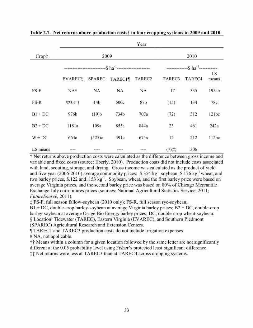
The net returns for the double-cropped barley-soybean system at average Virginia prices

ranged from $(72) to 976 ha-1, with an average return of $440 ha-1 (Table 2.7). The net returns

23

for the double-cropped barley-soybean system at Osage Bio Energy prices ranged from $23 to

1181 ha-1 (Table 2.7), with an average return of $579 ha-1. The double-cropped wheat-soybean

system net returns ranged from $(525) to 674 ha-1 (Table 2.7), with an average return of $255

ha-1. The full-season rye-soybean system net returns ranged from $(15) to 525 ha-1 (Table 2.7)

with an average return of $207 ha-1, while the full-season fallow-soybean system had an average

return of $176 ha-1 on the two TAREC locations in 2010.

In both years, the barley-soybean system at Osage Bio Energy prices had the greatest net

returns at every location, although returns were not always significantly different (Table 2.7). In

2009, the barley-soybean system net returns at average Virginia prices were less than the barley-

soybean system net returns at Osage Bio Energy prices at three of four locations, but greater than

or equal to the net returns from the full-season rye-soybean and double-crop wheat-soybean

systems at every location. The full-season rye-soybean had lower net returns than the Osage Bio

Energy barley-soybean system at every location, and the double-crop wheat-soybean system was

lower than the Osage Bio Energy barley-soybean system at three of four locations. In 2010,

TAREC4 had greater net returns than TAREC3 across cropping systems. The Osage Bio Energy

barley-soybean system net returns were greater than every other cropping system except full-

season fallow-soybean across locations (Table 2.7).

Our data indicate that an average of 43% of the wheat-soybean system total returns was

due to wheat: 39, 43, 37, and 39% at EVAREC, SPAREC, TAREC1, and TAREC2, respectively

in 2009, and 56 and 41% at TAREC3 and TAREC4, respectively in 2010. In a Mississippi

study, Kyei-Boahen and Zhang (2006) reported an average of 68% of the returns of a wheat-

soybean double-crop system were due to wheat in 2001, 2002, and 2004. The average wheat

yield reported by the authors was 5170 kg ha-1 compared to our average yield of 3386 kg ha-1. In

24

addition, the percentage of net returns contributed by wheat in a wheat-soybean double-crop

system has been less over the last several years due to greater soybean prices. In the Mississippi

study, soybean prices averaged $.192 kg-1 over the three years compared to Virginia’s 2006-2010

average price of $.354 kg-1. At statewide Virginia barley prices, an average of 37% of the

barley-soybean system total net returns was due to barley: 37, 47, 26, and 29% at EVAREC,

SPAREC, TAREC1, and TAREC2, respectively in 2009, and 45 and 36% at TAREC3 and

TAREC4, respectively in 2010. Our data show that at Osage Bio Energy barley prices, an

average of 42% of the barley-soybean system total net returns was due to barley: 42, 52, 30, and

34% at EVAREC, SPAREC, TAREC1, and TAREC2, respectively in 2009, and 50 and 45% at

TAREC3 and TAREC4, respectively in 2010.

Future research should repeat these comparisons to further establish yield trends. The net

returns data presented might change significantly with different yields, and therefore a different

growing season. Our data shows the barley-soybean double-cropped system as being generally

more profitable than either the full-season soybean or wheat-soybean double-cropped systems.

These conclusions need to be taken in context with the volatile weather and commodity markets

present during the time of this experiment. It is important to keep in mind that the prices used

are long-term averages, and short-term management decisions might use spot prices that differ

significantly. It will be interesting to see how additional research will compare with the results

presented here.

25

REFERENCES

Alley, M.A., P. Scharf, D.E. Brann, W.E. Baethgen, and J.L. Hammons. 2009a. Nitrogen

Management for Winter Wheat: Principles and Recommendations. Ext. Pub. 424- 026.

VA Coop. Ext., Virginia Tech, Blacksburg. Available at: http://pubs.ext.vt.edu/424/424-

026/424-026.html [Accessed 16 March 2011].

Alley, M.A., T.H. Pridgen, D.E. Brann, J.L. Hammons, and R.L. Mulford. 2009b. Nitrogen

Fertilization of Winter Barley: Principles and Recommendations. Ext. Pub. 424-801. VA

Coop. Ext., Virginia Tech, Blacksburg. Available at: http://pubs.ext.vt.edu/424/424-


Camper, H.M., Jr., Genter, C.F., and Loope, K.E. 1972. Double cropping following winter barley

harvest in eastern Virginia. Agron. J. 64:1-3.

Eberly, Eric. 2010. BUDSYS: Enterprise Budget System Generator user’s manual. VA Coop.


FutureSource. 2011. Interactive Data Desktop Solutions. Available at:

http://futuresource.quote.com/charts/home.action [Accessed 15 February 2011].

Groover, G.E., Kenyon, D.E., and Kramer, R.A. 1989. An evaluation of production and

marketing strategies for eastern Virginia cash grain producers. Ext. Pub. 89-1. VA

Coop. Ext., Virginia Tech, Blacksburg.

Herbek, J.H., and M.J. Bitzer. 1998. Soybean production in Kentucky part III: planting

practices and double cropping. Ext. Pub. AGR-130. Coop. Ext. Serv., University of

Kentucky. Available at: http://www.ca.uky.edu/agc/pubs/agr/agr130/agr130.htm

[Accessed 23 February 2011].

Herbert, Ames, and Scott Hagood. 2011. Pest Management Guide: Field Crops, 2011.

26

Ext. Pub. 456-016. VA Coop. Ext., Virginia Tech, Blacksburg. Available at

http://www.pubs.ext.vt.edu/456/456-016/456-016.html [Accessed 27 April 2011].

Holshouser, D.L. 2010. Suggested soybean seeding rates for Virginia. Ext. Pub. 3006-1447. VA

Coop. Ext., Virginia Tech, Blacksburg. Available at: http://www.pubs.ext.vt.edu/3006/

3006-1447/3006-1447.html [Accessed 21 April 2011].

Kelley, K.W. 2003. Double-cropping winter wheat and soybean improves net returns in the

eastern Great Plains. Online. Crop Management doi: 10.1094/CM-2003-1112-01-RS.

Kyei-Boahen, S., and Zhang, L. 2006. Early-maturing soybean in a wheat- soybean double-crop

system: yield and net returns. Agron. J. 98:295-301.

LeMahieu, P.J., and M.A. Brinkman. 1990. Double-cropping soybean after harvesting small

grains as forage in the North Central USA. J. Prod. Agric. 3:385-389.

National Agricultural Statistics Service. 2011. Crops state data [Online]. Available at:

http://www.nass.usda.gov/QuickStats/Create_Federal_All.jsp [Accessed 23

February 2011]. USDA-NASS, Washington, D.C.

Sanford, J.O., Eddleman, B.R., Spurlock. S.R., and J.E. Hairston. 1986. Evaluating ten

cropping alternatives for the midsouth. Agron. J. 78:875-880.

SAS Institute. 2008. The SAS system for Windows. Release 9.2. SAS Inst, Cary, NC.

Simpson, T.W., S.J. Donohue, G.W. Hawkins, M.M. Monnett, and J.C. Baker. 1993. The

development and implementation of the Virginia Agronomic Land Use Evaluation

System (VALUES). Department of Crop and Soil Environmental Sciences, Virginia

Tech, Blacksburg, VA.

27

Soil Survey Staff, Natural Resources Conservation Service, US Department of Agriculture.

Official Soil Series Descriptions [Online]. Available at: http://soils.usda.gov/technical/

classification/osd/index.html [Accessed 22 February 2011]. USDA-NRCS, Lincoln, NE.

Virginia Soil and Water Conservation. 2005. Virginia Nutrient Management Standards and

Criteria, Revised October 2005. Virginia Department of Conservation and Recreation,

Richmond.

Wesley, R.A. 1999. Double cropping wheat and soybeans. P. 143-156. In L.G. Heatherly and

H.F. Hodges (ed.) soybean production in the midsouth. CRC Press, Boca Raton, FL.

Wesley, R.A., Heatherly, L.G., Elmore, C.D. and Spurlock, S.R. 1994. Net returns from eight

irrigated cropping systems on clay soil. J. Prod. Agric. 7:109-115.

Wesley, R.A., Heatherly, L.G., Elmore, C.D., and Spurlock, S.R. 1995. Net returns from eight

nonirrigated cropping systems on clay soil. J. Prod. Agric. 8: 514-520.

28

Table 2.1. Soil series and yield potential† for 2009 and 2010 experimental locations.

Yield potential† Year

Location‡

Soil series

Corn

Barley

Wheat

Soybean (early / late)§

-----------------kg ha 1-----------------

2009

EVAREC

Kempsville

8780

4730

4700

2690 / 2280

SPAREC

Appling

7525

4730

4700

2350 / 1680

TAREC1

Eunola

8150

4730

4700

2690 / 2280

TAREC2

Rains (drained)

10660

4730

4700

3020 / 2280

2010

TAREC3

Nansemond¶

10030

6180

5375

2690 / 2280

TAREC4

Dragston

10030

6180

5375

2690 / 2280

† All yield potentials based on VALUES, Virginia Agronomic Land Use Evaluation System (Simpson, 1993; Virginia Soil and Water Conservation, 2005). ‡ Location: Tidewater (TAREC), Eastern Virginia (EVAREC), and Southern Piedmont (SPAREC) Agricultural Research and Extension Centers. § Late season soybean assumed planted on or after 21 June. ¶ Yield potentials do not correspond to those experienced at the TAREC in numerous experiments. The Nansemond is a loamy find sand whose subsoil consists of sandy loam from 20 to 74 cm then becomes a loamy fine sand to 168 cm, where it changes to a sand. Yields in the City of Suffolk Soil Survey lists the soil as yielding 672 and 336 kg ha-1 less than a Dragston and similar to the Eunola. We think that this soil has less yield potential than any soil listed except for the Appling.

29

Table 2.2. Locations and small grain cultivars used at various planting dates for the 2008-2009 and 2009-2010 growing seasons.

Planting date Year

Location†

Thoroughbred barley

SS520 wheat

2008-2009

EVAREC

15 Oct. 2008

12 Nov. 2008

SPAREC

16 Oct. 2008

6 Nov. 2008

TAREC1

14 Oct. 2008

3 Nov. 2008

TAREC2

10 Oct. 2008

3 Nov. 2008

2009-2010

TAREC3

20 Nov. 2009

20 Nov. 2009

TAREC4

23 Oct. 2009

23 Oct. 2009

† Location: Tidewater (TAREC), Eastern Virginia (EVAREC), and Southern Piedmont (SPAREC) Agricultural Research and Extension Centers.

30

Table 2.3. Locations, soybean cultivars, and planting dates for full-season and double-crop systems in 2009 and 2010.

Planting date Year

Location†

Cultivars

FS-F‡

FS-R

DC-B

DC-W

2009

EVAREC

Asgrow AG4907

----

27 May

8 June

23 June

SPAREC

Asgrow AG5605

----

21 May

9 June

22 June

TAREC1

Pioneer 95Y70

----

21 May

4 June

17 June

TAREC2

Asgrow AG4907

----

21 May

2 June

11 June

2010

TAREC3

Asgrow AG5605

21 May

21 May

3 June

17 June

TAREC4

Asgrow AG4907

22 May

22 May

3 June

17 June

† Location: Tidewater (TAREC), Eastern Virginia (EVAREC), and Southern Piedmont (SPAREC) Agricultural Research and Extension Centers. ‡ FS-F, full season fallow-soybean (2010 only); FS-R, full season rye-soybean; DC-B, double-crop barley-soybean; DC-W, double-crop wheat-soybean. Table 2.4. Analysis of variance for small grain and soybean yields in full-season and double-crop systems in 2009 and 2010.

2009

2010 Effect

Small grain

Soybean

Small grain

Soybean

P value

CS†

<0.0001

<0.0001

0.0012

0.6459

Location

<0.0001

<0.0001

0.0138

<0.0001

CS x Location

<0.0001

0.0001

0.1370

0.4575

† Cropping System.

31

Table 2.5. Barley, wheat, and soybean yields in four cropping systems in 2009 and 2010.

Year

2009

2010 Crop†

EVAREC‡

SPAREC

TAREC1

TAREC2

TAREC3

TAREC4

LS means

-------------------------kg ha-1--------------------

---------------kg ha-1-----------

Small Grain

Barley

6766a§

4220a

3987a

4515a

3820

4918

4369a

Wheat

4463b

1448b

3492a

4359a

3109

3442

3276b

LS means

----

----

----

----

3465b¶

4180a

Soybean

FS-F

NA††

NA

NA

NA

1648

2710

----

FS-R

3613ab

1822a

3536b

2158b

1818

2316

----

DC-B

3984a

1676a

4165a

3616a

1690

2630

----

DC-W

3522b

996b

3210c

3376a

1589

2467

----

LS means

----

----

----

----

1686‡‡

2593

† FS-F, full season fallow-soybean (2010 only); FS-R, full season rye-soybean; DC-B, double-crop barley-soybean; DC-W, double-crop wheat-soybean. ‡ Location: Tidewater (TAREC), Eastern Virginia (EVAREC), and Southern Piedmont (SPAREC) Agricultural Research and Extension Centers. § Means within a column for a given location followed by the same letter are not significantly different at the 0.05 probability level using Fisher’s protected least significant difference. ¶ Small grain yielded less at TAREC3 than at TAREC2 across cropping systems. †† NA, not applicable. ‡‡ Soybean yielded less at TAREC1 than at TAREC2 across cropping systems.

32

Table 2.6. Analysis of variance for barley, wheat, and soybean net returns in full-season and double-crop systems in 2009 and 2010. Effect

2009

2010

P value

Cropping System

<0.0001

0.0254

Location

<0.0001

<0.0001

Cropping System x Location

<0.0001

0.0752

33

Table 2.7. Net returns above production costs† in four cropping systems in 2009 and 2010.

Year

Crop‡

2009

2010

-------------------------$ ha-1--------------------

-------------$ ha-1-----------

EVARECξ

SPAREC

TAREC1¶

TAREC2

TAREC3

TAREC4 LS

means FS-F

NA#

NA

NA

NA

17

335

195ab

FS-R

523d††

14b

500c

87b

(15)

134

78c

B1 + DC

976b

(19)b

734b

707a

(72)

312

121bc

B2 + DC

1181a

109a

855a

844a

23

461

242a

W + DC

664c

(525)c

491c

674a

12

212

112bc

LS means

----

----

----

----

(7)‡‡

306

† Net returns above production costs were calculated as the difference between gross income and variable and fixed costs (source: Eberly, 2010). Production costs did not include costs associated with land, scouting, storage, and drying. Gross income was calculated as the product of yield and five-year (2006-2010) average commodity prices: $.354 kg-1 soybean, $.176 kg-1 wheat, and two barley prices, $.122 and .153 kg-1. Soybean, wheat, and the first barley price were based on average Virginia prices, and the second barley price was based on 80% of Chicago Mercantile Exchange July corn futures prices (sources: National Agricultural Statistics Service, 2011; FutureSource, 2011). ‡ FS-F, full season fallow-soybean (2010 only); FS-R, full season rye-soybean; B1 + DC, double-crop barley-soybean at average Virginia barley prices; B2 + DC, double-crop barley-soybean at average Osage Bio Energy barley prices; DC, double-crop wheat-soybean. § Location: Tidewater (TAREC), Eastern Virginia (EVAREC), and Southern Piedmont (SPAREC) Agricultural Research and Extension Centers. ¶ TAREC1 and TAREC3 production costs do not include irrigation expenses. # NA, not applicable. †† Means within a column for a given location followed by the same letter are not significantly different at the 0.05 probability level using Fisher’s protected least significant difference. ‡‡ Net returns were less at TAREC3 than at TAREC4 across cropping systems.

34

Figure 2.1. Maximum and minimum temperatures and rainfall† at EVAREC, SPAREC, and TAREC in 2009, and TAREC in 2010.

35

Fig. 4.3. Continued.

†TAREC rainfall does not include 50 mm of irrigation on 15 July 2009 and 25 mm on two occasions on 1 and 20 July 2010.

36

Chapter 3 – Breakeven Sensitivity Analysis of Full-Season and Double-Cropped

Soybean Systems

Introduction

Full-season soybean and soybean grown after wheat are the predominant soybean

cropping systems in the Mid-Atlantic. A barley-based ethanol plant recently built in Virginia is

increasing demand for locally grown barley. Very little information is available comparing a

barley-soybean system to either full-season soybean or wheat-soybean cropping systems.

Virginia studies are outdated and new data is needed. This paper describes a model that can be

used to determine breakeven prices among these different cropping systems. Double-cropped

systems are generally more efficient than mono-cropped systems because some costs, such as

lime, land rent, or machinery depreciation, which remain independent of cropping system, will

be more spread out because of the increased crop production per acre. Production practices

between the double-cropped wheat-soybean and double-cropped barley-soybean systems are

assumed to be virtually the same and will require no additional equipment.

What does a breakeven number represent?

The breakeven number is the sales value at which one enterprise has net returns equal to

another enterprise. This principle is universal across financial and business fields, and is

applicable to many areas aside from agriculture. The specific comparisons addressed in this

paper are all soybean rotations. First, it is assumed that the price is held constant for soybean

double-cropped after barley or wheat. Once this assumption is made, a breakeven price can be

calculated for wheat and barley. That is, the breakeven price per bushel needed for wheat so that

the net returns from a wheat-soybean double-cropped system is equal to the net returns from a

37

barley-soybean double-cropped system. Conversely, the price per bushel for barley can be

calculated in the same manner. Breakeven prices can also be calculated for wheat or barley in a

double-cropped system versus full-season soybean. If a farmer currently only grows full-season

soybean, a comparison with either double-cropped system would be helpful when making a

rotation decision.

Furthermore, the model can be used at any time of the year. This aspect would be useful

when making management decisions in response to major changes in prices or yield during the

growing season. For example, if the prices for a small grain decrease near harvest, a grower

could determine if the net returns would be worth the cost of harvesting the small grain.

Breakeven prices for corn (or any other crop) can also be calculated and compared to these or

any other rotation using the principles outlined here. It is assumed that while there may be

marginal acreage differences between crops planted on an annual basis, farmers will not plant all

of their land with one crop; therefore, only soybean cropping systems are included in this model.

Breakeven values can be calculated for any other factor as well, such as yield or a specific

variable cost. For example, if yields for wheat or barley were anticipated to be poor, breakeven

yields could be compared with the net returns from the full-season soybean to justify harvesting

the small grain crop; however, only breakeven prices are included in this model.

How is this useful?

Breakeven prices are useful as a management tool. Making sound production decisions is

one of the most important responsibilities of a farm manager. Profitability is one of the primary

goal of any business, so it makes sense that growers will select crop rotation to support a more

profitable business. Breakeven tables allow the user to compare the prices needed for an

38

alternative enterprise to be as profitable as the status quo. By using this model, the user will

understand what is required for a crop rotation to be more profitable.

What values are needed?

The formula used in this model to calculate net returns for double-cropped systems is as

follows:

Eq. 1: (PB)*(YB) + (PSB)*(YSB) – (VCB + VCSB) = (PW)*(YW) + (PSB)*(YSB) – (VCW + VCSB)

Where PB , PW , PSB = Price of Barley, Wheat, and Soybean YB , YW , YSB = Yield of Barley, Wheat, and Soybean VCB , VCW , VCSB = Variable Costs of Barley, Wheat, and Soybean

The left-hand side of equation 1 is the net returns of the barley-soybean system:

(PB)*(YB) + (PSB)*(YSB) – (VCB + VCSB)

Gross income for barley is defined by (PB)*(YB), and gross income of soybean following barley

is defined as (PSB)*(YSB). The sum is the total gross income of the double-cropped barley-

soybean system. Next, (VCB + VCSB) is equal to the variable costs of growing both the barley

and the soybean. Subtracting the variable cost from the gross income equals net returns over

variable cost, defined as net returns for the remainder of this discussion.

The right-hand side of equation 1 is the net returns of the wheat-soybean system:

(PW)*(YW) + (PSB)*(YSB) – (VCW + VCSB)

Gross income for wheat is defined by (PW)*(YW), and gross income of soybean following wheat

is defined as (PSB)*(YSB). The sum is the total gross income of the double-cropped barley-

soybean system. Finally, (VCW + VCSB) is the variable cost of the entire system. The full-season

soybean net returns are calculated in a similar manner, except net returns are determined for only

the soybean crop. Once the net returns are known, the full-season soybean can be compared with

either double-cropped system.

39

Variable Costs vs. Fixed Costs

The idea of using variable costs only is an important assumption, and needs to be

discussed in more detail. Production expenses are usually split into two categories: variable

costs and fixed costs. Fixed costs are incurred no matter the enterprise. These include, but are

not limited to, expenses such as depreciation, management, operator labor, and equity capital.

Variable costs, on the other hand, include expenses specific to the enterprise. These include such

things as fertilizer, fuel, seed, chemicals, and hired labor.

When comparing a wheat-soybean rotation with a barley-soybean rotation, it is assumed

that fixed costs will be the same for both enterprises. For example, the farmer’s machinery

depreciation (a fixed cost) is going to be the same whether barley or wheat is grown. On the

other hand, seed cost (a variable cost) will be different for the two crops. Land rental rates and

other costs that are not dependent on cropping system are not included. These costs need to be

taken into account when making long-term cropping decisions, but are beyond the scope of this

model. Individual growers can plug in their own fixed cost numbers to consider returns to all

costs.

Example Calculation

This section goes over an example breakeven calculation using values taken from the

example enterprise budgets in Appendix C. Prices are the median commodity values available at

Petersburg and Hopewell from 2006 to 2010 (Appendix B). Yield estimates are based on

Virginia yield trials and unpublished experimental data (D.L. Holshouser, Personal Commun-

ication, 2011). Assumptions used are as follows:

40

Barley-Soybean Rotation PB = $3.19; YB = 90 bu/ac

PSB = $9.19; YSB = 33 bu/ac

VCB + VCSB = $377.26 /ac

Return over Variable Costs = (3.19 x 90) + (9.19 x 32) – (375.46) = $213.11

Wheat-Soybean Rotation PW = $4.08; YW = 70 bu/ac

PSB = $9.19; YSB = 26 bu/ac

VCW + VCSB = $408.75

Return over Variable Costs = (4.08 x 70) + (9.19 x 26) – 408.75 = $115.79

The breakeven price of wheat is solved as follows:

(PW x 70) + (9.19 x 26) – 408.75 = 213.11

(PW x 70) + 238.94 – 408.75 = 213.11

(PW x 70) = 213.11 + 408.75 – 238.94

PW x 70 = 382.92

PW = 375.53 / 70 = $5.47

Therefore, $5.47 is the price needed for wheat to breakeven with barley when barley is $3.19.

Likewise, the breakeven price of barley:

(PB x 90) + (9.19 x 33) – 377.26 = 115.79

(PB x 90) + 303.27 – 377.26 = 115.79

(PB x 90) = 115.79 + 377.26 – 303.27

(PB x 90) = 189.78

PB = 189.78 / 90 = $2.11

Here, $2.11 is the price needed for barley to breakeven with wheat when wheat is $4.08. In

addition to breakeven prices, barley, wheat, and soybean breakeven yields or variable costs can

also be calculated in the same manner, although they are not included in this model.

41

Explanation of the Excel Model

The breakeven calculations are estimates based on historical values and growers should

incorporate personal knowledge into their individual analysis. When the spreadsheet is opened

the first tab is labelled ‘Table of Contents’. This sheet serves as a navigation tool for the rest of

the model. To calculate breakeven prices follow the individual steps listed on this sheet. If any

tabs are mentioned that are not listed they can be accessed by clicking on the ‘Index’ link at the

bottom of this first sheet. This will take you to an index of all tabs used in the model with links

to each. However, only the steps listed in the ‘Table of Contents’ tab are absolutely necessary to

use the program.

The first step asks for verification of the production costs as listed in the individual

budgets. Clicking on the ‘Corn Budget’ link will take you to the enterprise budget used

specifically for the corn crop. Here any changes in prices of seed, fertilizer, labor, etc. can be

made. Note that prices and yields at the top of the budget are not changed here; this will be done

later. The corn budgets are not used in the breakeven calculations for the soybean systems, but

will be listed in the ‘Summary Table’ to provide context for the overall rotation. Once finished,

click on ‘Return to Table of Contents’ and you will be redirected to the first page. Follow the

same process for the ‘Full-Season Soybean Budget’, ‘Barley-Soybean Double-Crop Budget’, and

‘Wheat-Soybean Double-Crop Budget’ links.

All of these budgets are derived from Virginia Cooperative Extension’s Enterprise

Budget System Generator (Budsys) (Eberly, 2010). All of the costs used in the budgets are

based on average 2010 operating expenses, as estimated by the Budsys computer program and

Virginia Tech Extension faculty. The user can adjust the enterprise budgets to reflect values

deemed most accurate for their farm. Estimated costs (both variable and fixed) are provided in

42

the tabs ‘Chemicals’, ‘Machinery’, ‘Seed’, and ‘Rates’. Note: Only costs should be changed in

the individual budgets. Prices and yields should be changed in the tab ‘Summary Table’ as will

explained later. If costs are changed in the individual budgets, the total variable costs and returns

over variable costs columns in the “Summary Table” will adjust automatically. It might be

noticed there are tabs labeled “Full-Season Avg. Budget”, “Barley DC Avg. Budget”, and

“Wheat DC Avg. Budget”. These budgets should not be adjusted, as they automatically use the

average prices described above to provide a reference point for the individual breakeven tables.

This will be explained later in more detail.

Excel Spreadsheet: Summary Table

The second step is to enter anticipated prices and yields. Click on the ‘Summary Table’

link. This takes you to a sheet that shows the prices, yields, variable costs, and returns over

variable costs for each enterprise. The breakeven analysis looks only at the full-season soybean,

barley-soybean, and wheat-soybean systems, but in this chart corn is also summarized to provide

context.

This is the only sheet in the model where the user must enter data. First, an elevator is

chosen. Obviously, a farmer might do business with any number of elevators. Here, Petersburg

and Tappahannock simply represent the two different barley pricing mechanisms. We assume

Osage Bio Energy will offer 80% of Chicago July corn prices for barley delivered to their

ethanol plant in Hopewell. The prices “local” to Hopewell for wheat, soybeans, and corn are

represented by the Petersburg prices. Presumably, if a grower has the means to ship barley to

Hopewell, the other crops can be shipped nearby to Petersburg. The other pricing mechanism is

barley delivered to one of several buy-in stations in Virginia and Maryland, including

43

Tappahannock. Osage Bio Energy will offer 80% of Chicago July corn futures less a $.25 per

bushel basis for barley delivered to a buy-in station. Presumably, if a grower will ship barley to

Tappahannock, the other crops can be shipped to Tappahannock as well. These two delivery

stations serve as reference points in this model.

Next, the summary table lists the enterprises being evaluated. In the second column, the

commodity prices need to be manually entered. The prices listed when the spreadsheet is first

opened reflect the 50th percentile of commodity prices at Petersburg for corn, wheat, and

soybeans from January 2006-December 2010 (Virginia Market News: Virginia Grain Prices and

Statistics, 2011). The barley price is the average barley price that would have been available if

Osage Bio Energy had been offering 80% of Chicago corn from January 2006-December 2010

(FutureSource, 2011). Regardless, at this point the user should enter the commodity prices

deemed to be most accurate for the individual operation. Once the full-season soybean price is

entered the two double-cropped soybean prices are automatically filled in for all soybean

regardless of the cropping system.

Once commodity prices are entered, the third column will automatically “look up” the

percentile of historical prices from either the tab ‘Petersburg Prices’ (January 2006-December

2010), or the tab ‘Tappahannock Prices’, which contains the monthly prices available at

Tappahannock from January 2006-December 2010. If the percentile is 50%, this is the value

where half the prices over the last five years have been higher and half have been lower. If the

percentile is 75%, prices have been greater 25% of the time over the last five years, but have

been less 75% of the time. This is where the elevator choice comes into play; the percentiles will

be slightly different at the two locations. This idea of a “percentile” price merely serves as a

reference point.

44

The fourth column is yield for each of the four cropping systems. These values need to

be manually entered. Keep in mind all three soybean yields should be different, as planting dates

will vary across the rotations. For instance, if barley is harvested in the first week of June,

soybean planted immediately after will have several weeks more growing time than soybean

planted after wheat in late June or early July. This is another key difference in the rotations: how

will planting date affect soybean yield?

The fifth column shows variable costs. These values do not need to be manually entered.

The variable costs are taken automatically from the individual enterprise budgets for each

cropping system, and, if necessary, should have been adjusted in the first step. The sixth and

final column in the ‘Summary Table’ tab shows the returns over variable costs. This is

calculated as shown above: price times yield less variable costs. This information is calculated

automatically given the numbers manually entered in the earlier columns. All of the values

needed are now available so the model can calculate breakeven prices. Click on ‘Return to Table

of Contents’.

Excel Spreadsheet: Breakeven Tables

The third step is interpreting the breakeven prices. Click on the link titled ‘Breakeven

Tables’. These breakeven tables are calculated using the data entered in the ‘Summary Table’

according to the breakeven equation. The first section in the ‘Breakeven Tables’ compares

“barley vs. wheat breakevens”. The upper table is discussed first. This breakeven table uses the

average prices and average enterprise budgets mentioned earlier. When price and yield data are

entered, the lower table will change to reflect the individual farm data, but this “average” table

will not. It serves as a standard against which to compare the second table.

45

The median price of $4.08 for wheat was shown earlier to equal $2.11 for barley

according to the previous assumptions, including $9.19 for soybeans. Of course, the median

price is almost never going to be the price offered, so a sensitivity analysis is needed. A

sensitivity analysis looks at how deviations in price away from the median will affect the

breakeven price. At less 25% of the median price wheat is $3.06, which in turn is reflected in a

lower barley breakeven price. At plus 25% of the median price wheat is $5.10, which is also

reflected in a higher barley breakeven price. “Less 25%” does not mean the 25th percentile; it

just means 75% of the median price ($4.08 x .75 = $3.06). Likewise, “Plus 25%” does not mean

the 75th percentile; it means 125% of the median price ($4.08 x 1.25 = $5.10). The lower part of

this table is read in a similar manner: the breakeven prices of wheat given the prices of barley

shown. The explanation of the table is also found beside it in the Excel spreadsheet.

The second table is what shows the breakeven numbers that reflect the prices and yields

manually entered in the ‘Summary Table’. It is calculated in the same way as the median values,

but is specific to the values the user has entered. All of these values are automatically calculated;

the ‘Summary Table’ is the only tab where values are required to be entered. When the

spreadsheet is first opened, the upper and lower breakeven tables are identical. This is because

the average values used in the sample calculation are the default values when the program is first

opened. Once the prices and yields are changed the lower table will change automatically, but

the upper table will keep using the median values.

The second step in the ‘Breakeven Tables’ compares “wheat vs. full-season soybean

breakevens”. The upper table uses the median prices and average enterprise budgets in the same

manner as the barley vs. wheat breakevens, except the average full-season soybean numbers are

used instead of the double-cropped barley-soybean numbers. The median price of $4.08 for

46

wheat is equal to $8.36 full-season soybean (when double-cropped soybean is $9.19), given the

calculation. Again, the median price is almost never going to be the price offered, so a

sensitivity analysis is needed. The lower part of this table is read in a similar manner: the

breakeven prices of wheat given the prices of full-season soybean shown. The explanation of the

table is also found beside it in the Excel spreadsheet. The lower table in this section shows the

breakeven numbers that reflect the prices and yields manually entered in the ‘Summary Table’.

The third step in the ‘Breakeven Tables’ compares “barley vs. full-season soybean

breakevens”. The upper table uses the median prices and average enterprise budgets in the same

manner as the wheat vs. full-season soybean breakevens, except the average double-cropped

barley-soybean numbers are used instead of the double-cropped wheat-soybean numbers. The

median price of $3.19 for barley is equal to $11.14 for full-season soybean (when double-

cropped soybean is $9.19), given the calculation. The lower part of this table is read in a similar

manner: the breakeven prices of wheat given the prices of full-season soybean shown. The

explanation of the table is also found beside it in the Excel spreadsheet. The lower table in this

section shows the breakeven numbers that reflect the prices and yields manually entered in the

‘Summary Table’.

Excel Spreadsheet: Summary Graph

The fourth and final part of the model is a visual representation of total cropping system

profitability. Click on the ‘Summary Graph’ link. Here, a bar graph reflects the returns over

variable costs as shown in the ‘Summary Table’. This is automatically created with the numbers

that are manually entered. Again, when the spreadsheet is first opened, the graph will reflect the

average default numbers. This tab is a visual representation of income flow.

47

Excel Spreadsheet: Index of Tabs

All of the tabs in the model are accessed by clicking on the ‘Index’ link on the ‘Table of

Contents’ sheet. An index of the spreadsheet tab links will be shown as below, in the order in

which they appear in the Excel file.

1) Table of Contents 2) Summary Table 3) Breakeven Tables 4) Summary Graph 5) Petersburg Prices 6) Tappahannock Prices 7) Corn Budget 8) Full-Season Budget 9) Full-Season Avg. Budget 10) Barley DC Budget 11) Barley DC Avg. Budget 12) Wheat DC Budget 13) Wheat DC AVg. Budget 14) Chemicals 15) Machinery 16) Seeds 17) Rates

48

Interpretations

The breakeven tables can provide support on selecting a profitable cropping system. For

instance, look at the first section of the breakeven tables that compares barley versus wheat.

Here, the breakeven prices for barley ($1.32, $2.11, and $2.90) are all less than the 50th

percentile barley price of $3.19. This implies that the barley-soybean system as a whole is

generally more profitable than the wheat-soybean system (assuming the yields entered in the

summary table and $9.19 for soybean). Likewise, the wheat breakeven prices ($4.45, $5.47, and

$6.50) are all higher than the 50th percentile wheat price of $4.08. This implies that the wheat-

soybean system is generally less profitable than the barley-soybean system.

Fig. 3.1. Wheat vs. Barley Breakeven Prices

Wheat Barley Less 25% $3.06 $1.32

Price $4.08 $2.11 Plus 25% $5.10 $2.90 Barley Wheat

Less 25% $2.39 $4.45 Price $3.19 $5.47

Plus 25% $3.99 $6.50

Next, look at the wheat versus full-season soybean breakevens (Fig. 3.2). When wheat is

$4.08 or $3.06, the breakeven soybean prices ($6.32 and $8.36) are below the 50th percentile

soybean price of $9.19. When wheat prices go up, in this example to $5.10, the breakeven

soybean price increases to $10.40, which is greater than $9.19. This indicates that at lower

wheat prices full-season soybean is more lucrative, but as wheat prices increase (into the range

where they are trading today) the double-cropped wheat-soybean system is more profitable.

Again, please bear in mind the assumptions that are being used, and that these interpretations

might change with different prices and yields.

49

Fig. 3.2. Wheat vs. Full-Season Soybean Breakeven Prices

Wheat Soybean Less 25% $3.06 $6.32

Price $4.08 $8.36 Plus 25% $5.10 $10.40 Soybean Wheat Less 25% $6.89 $3.35

Price $9.19 $4.50 Plus 25% $11.49 $5.65

Finally, the third part of the breakeven tables examines barley versus full-season soybean

breakevens (Fig. 3.3). At the lower barley price of $2.39, the soybean breakeven price is $9.09,

which is below the $9.19 50th percentile price. As the barley prices increase to $3.19 then to

$3.99, the soybean prices are higher than the $9.19. This indicates that at very low barley prices

the full-season soybean system is more profitable. Incidentally, this is the range where barley

prices have been in Virginia for a long time. When the barley prices increase into the range

where they exist today, the double-cropped barley-soybean system is more profitable. Again on

the lower chart, a barley-soybean system appears to be more profitable except at very high full-

season soybean prices.

Fig. 3.3. Barley vs. Full-Season Soybean Breakeven Prices

Barley Soybean Less 25% 2.39 9.09

Price 3.19 11.14 Plus 25% 3.99 13.19 Soybean Barley Less 25% 6.89 1.54

Price 9.19 2.43 Plus 25% 11.49 3.33

50

Profitability Scenarios

This model can be used in other ways aside from the breakeven sensitivity analysis as

well. The summary table can be used to compare the initial profitability over variable costs of

the different systems. This is particularly helpful when making short-term management

decisions that compare prices that are available to the individual using the program. The

breakeven tables use five-year prices, so that aspect provides interpretations for more long-term

decisions. A comparison is easily done by comparing the returns over variable costs as listed in

the summary table. Going forward with the idea of percentile prices, commodities can be

compared at different levels of sales value. The prices used in this scenario are taken from

Petersburg soybean and wheat and Hopewell barley as listed in Table 3.1. The crop yield

assumptions are 90 and 70 bushels per acre for barley and wheat, respectively. The full-season

soybean yield is a base yield, with soybean after barley as 90% of full-season yield and soybean

after wheat as 75% of full-season yield. Once all these assumptions are made, total system

profitability can be compared as seen in Table 3.2 on the next page.

Table 3.1. Five-year soybean, barley, and wheat prices at various percentiles.

Price percentiles Crop

10th

25th

50th

75th

90th

$ / bushel

Soybean

5.65

7.13

9.19

10.90

12.87

Barley

2.02

2.84

3.19

3.59

4.80

Wheat

3.11

3.72

4.08

6.02

7.44

51

Table 3.2. Full-season soybean, double-cropped barley-soybean, and double-cropped wheat-soybean system profitability at various yields and prices.

Full-season soybean yields (bu/ac) Percentile Price

Cropping System

30

40

50

60

70

---------------------$ / acre----------------------

10th

Full-Season Soybean

(0.27)

42.36

84.99

127.62

170.24

Barley-Soybean

(25.97)

12.31

54.44

92.17

134.30

Wheat-Soybean

(57.26)

(27.74)

6.19

35.21

69.64

25th

Full-Season Soybean

44.13

101.56

158.99

216.42

273.84

Barley-Soybean

90.75

142.35

199.28

250.33

307.26

Wheat-Soybean

19.48

59.36

105.13

144.51

190.78

50th

Full-Season Soybean

105.93

183.96

261.99

340.02

418.04

Barley-Soybean

181.99

252.13

329.66

399.25

476.78

Wheat-Soybean

92.06

146.36

208.61

262.41

325.16

75th

Full-Season Soybean

157.23

252.36

347.49

442.62

537.74

Barley-Soybean

267.58

353.11

447.74

532.72

627.35

Wheat-Soybean

267.19

333.46

409.39

475.16

551.59

90th

Full-Season Soybean

216.33

331.16

445.99

560.82

675.64

Barley-Soybean

433.61

536.87

651.20

753.91

868.24

Wheat-Soybean

411.90

491.96

583.65

663.21

755.40

52

Table 3.2 provides some interesting food for thought. At the lowest prices and lowest

yields none of the systems are profitable (keeping in mind that crop insurance revenue is not

included in the budgets). At the lowest prices and highest soybean yields, full-season soybean is

the most profitable. This is because the full-season soybean has a lower variable cost to

overcome to be profitable. As the prices increase this quickly changes to the barley-soybean

system as the additional income from the barley crop begins to show. At median prices and

median soybean yields, the barley-soybean system is still the most profitable, but the differences

between full-season soybean and wheat-soybean are interesting. At the 50th percentile full-

season soybean is more profitable than the wheat-soybean system because the wheat-soybean

system has a high variable cost, but as prices go up the wheat-soybean system replaces the full-

season soybean. Here, the barley-soybean system is more profitable, but if farmers spread out

their risk with another cropping system, which should they choose? A small variation in prices

or yields could make one appear better than the other. There is no clear answer here. Obviously,

all farmers (and farms) have different yield potentials and market their crops in different ways,

so the trend of barley acreage over the next couple of years should be a clear indicator of how

growers are responding to the changing dynamics of Virginia commodity markets.

53

REFERENCES

Eberly, Eric. 2010. BUDSYS: Enterprise Budget System Generator user’s manual. VA Coop.


FutureSource. 2011. Interactive Data Desktop Solutions. Available at:

http://futuresource.quote.com/charts/home.action [Accessed 15 February 2011].

Virginia Market News: Virginia Grain Prices and Statistics. 2011. Virginia Department of

Agriculture and Consumer Services. Available at:

http://www.vdacs.virginia.gov/marketnews/grainstats.shtml [Accessed 16 April 2011]

54

Chapter 4 – Soybean Planting Date and Small Grain Residue Effects

on Soybean Yield and Yield Components

ABSTRACT

Full-season soybean [Glycine max (L.) Merr.] and double-cropped soybean following

wheat (Triticum aestivum L.) or barley (Hordeum vulgare L.) are three soybean cropping

systems used in the Mid-Atlantic USA. Research comparing these systems is limited; therefore,

field studies were conducted to determine the effect of planting date and winter grain on soybean

yield and yield components. Soybean yields declined with planting date at two of four locations

in 2009, a year that late-season rainfall enabled later-planted soybean to yield more than is

expected. Across these two locations, yield ranged from 1676 to 3887 kg ha-1 for the May and

early June planting dates, and declined to 905 to 3166 kg ha-1 by the mid-July planting date.

Soybean yield declined with planting date at 74 or 12 kg ha-1 less per week at the two locations.

Winter grain did not affect soybean yield in either year. These data indicate that planting date

has a greater effect on yield than the small grain residue. The yield component data reinforced

these results and indicated that the seed yield decline with later planting dates is due largely to a

decrease in the number of pods, which decreased an average of 29 or 56 pods m-2 per week at

each location in 2010.

55

INTRODUCTION

Soybean planting date is one of the most important factors related to agronomic yield.

Research methodology of soybean crop rotation and planting date has varied greatly across the

United States, but scientists have generally concluded that critical planting dates exist after

which soybean yields begin to decline. In the Mid-Atlantic USA, soybean is usually planted in

May as a full-season crop or in late-June to early-July as a double-crop after winter wheat. A

recent increase in the demand for barley presents double-crop soybean planted in early-June as a

third cropping system.

It is well documented that the later soybean is planted, the lower the seed yield. This has

been demonstrated most recently in Nebraska by Bastidas et al. (2008), in South Carolina by

Chen and Wiatrak (2010), and in Iowa by De Bruin and Pedersen (2008). Egli and Cornelius

(2009) summarized fifty years of planting date research in the Midwest, Upper South, and Deep

South regions of the United States, but did not include any Virginia studies. Their analysis

concluded that soybean yield is constant in early May, but begins to decline after May 30th in the

Midwest, June 7th in the Upper South, and May 27th in the Deep South. New agronomic data

describing soybean yield decline over time is needed in the Mid-Atlantic and Virginia in

particular.

In Nebraska, Bastidas et al. (2008) looked at soybean yield decline over four planting

dates from late-April to mid-June. In their experiment, soybean yield declined linearly from the

earliest planting dates. In Iowa, De Bruin and Pedersen (2008) also examined soybean yield

decline over four planting dates from late April to Mid-June and concluded that soybean yield

begins declining at an increasing rate after the earliest planting dates. In South Carolina, Chen

and Wiatrak (2010) studied soybean yield decline over seven planting dates from late-April to

56

mid-July. They found that soybean yield generally begins to decline by mid-June regardless of

maturity group, but is very dependent on growing conditions. In all of these studies soybean was

mono-cropped; none was planted after small grain. Other research has shown that the yield

decline with later planting dates is primarily due to decreased pods m-2, as shown most recently

by Pedersen and Lauer (2004) in Wisconsin and Robinson et al. (2009) in Indiana.

In addition to planting date, the effect of small grain residue may be partially responsible

for lower soybean yields following small grain. Yields may be lower due to the removal of soil

moisture by the small grain crop, leaving an inadequate supply for the succeeding soybean crop.

Or, other factors such as allelopathy may be involved. Allelopathy originally encompassed all

types of biochemical interactions between plants, both positive and negative (Molisch, 1937).

More recently it has come to be associated primarily with the negative effects one plant has on

another (Rice, 1984). This has long been associated with residue left on the soil surface from a

previous crop (Collison and Conn, 1925). Little is known about the variation in soybean yield

decline after different small grains.

Information describing the decline of soybean yield with planting date is well

documented, but less research of this nature has been conducted in Virginia. Even less data is

available comparing the soybean yield decline with delayed planting following different small

grain crops. The objectives of this study were to (i) describe the rate of yield decline for full-

season soybean, double-cropped barley-soybean, and double-cropped wheat-soybean systems as

planting date is delayed, and (ii) describe differences in soybean yield components as planting is

delayed in these cropping systems, and (iii) determine the effect of small grain residue on

soybean yield response to planting date.

57

MATERIALS AND METHODS

Experiments were conducted at four locations from fall 2008 through fall 2010: the

Eastern Virginia Agricultural Research and Extension Center (EVAREC) near Warsaw on a

Kempsville loam (fine-loamy, siliceous, subactive, thermic typic hapludults), the Southern

Piedmont Agricultural Research and Extension Center (SPAREC) near Blackstone on an

Appling fine sandy loam (fine, kaolinitic, thermic typic kanhapludults), and four experiments at

the Tidewater Agricultural Research and Extension Center (TAREC1-TAREC4) near Suffolk,

Virginia. A Eunola loamy fine sand (fine-loamy, siliceous, semiactive, thermic aquic hapludults)

and Rains fine sandy loam (fine-loamy, siliceous, semiactive, thermic, typic paleaquults) (tile-

drained) represented the soils at TAREC1 and TAREC2 during the 2008-2009 growing season,

respectively. In the 2009-2010 growing season, Nansemond loamy fine sand (coarse-loamy,

siliceous, subactive, thermic aquic hapludults) and Dragston fine sandy loam (coarse-loamy,

mixed, semiactive, thermic aeric endoaquults) (tile-drained) represented the soils at TAREC3

and TAREC4, respectively. The soil yield potentials for all sites are shown in Table 4.1.

Drought, poor emergence, and poor growth during the 2010 growing season prevented accurate

data collection at EVAREC and SPAREC; therefore, results from these experiments are not

included.

The experimental design for the first growing season was a randomized complete block

with four replications and arranged as a split-plot. Main plots were the winter small grains rye,

barley, or wheat. Rye was treated as a cover crop and killed with herbicide in early May. Barley

and wheat were harvested for grain. Subplots were planting date, with the initial planting date

for soybean following rye in May, or immediately following wheat or barley harvest (Table 4.2).

In 2009-2010, the experimental design was a randomized complete block arranged as a strip-plot

58

and replicated four times. Horizontal plots were the same winter small grains rye, barley, or

wheat plus an additional treatment with no small grain crop. Vertical plots were planting date,

with the initial planting dates for all plots in May and progressing weekly, resulting in a total of

nine planting dates (Table 4.3). Winter grain plots planted to soybean before wheat or barley

harvest were treated as cover crops and sprayed with herbicide one to two weeks before the

expected soybean planting date. Previous crop residue was corn at all sites except TAREC3,

where cotton was grown the previous year.

The barley and wheat cultivars at all locations in both years were Thoroughbred (Virginia

Crop Improvement Association, Richmond, VA) and SS520 (Southern States Cooperative,

Richmond, VA), respectively. Soybean cultivars for each location in both years are shown in

Tables 4.2 and 4.3. Soybean cultivar 95Y70 (Pioneer Hi-Bred, Int’l, Johnston, IA) is a maturity

group V and contains resistance to root knot nematode (Melooidogyne spp.), which was known

to be present in low numbers at TAREC1 in 2009. AG4907 (Monsanto Co., St. Louis, MO) is a

maturity group IV cultivar, and was used to facilitate earlier harvest on TAREC2 and TAREC4,

fields that can become wet during November and inhibit timely harvest. Otherwise, AG4907 and

AG5605 are both considered high-yielding cultivars of the most adapted maturity group at their

respective locations.

Fields were limed and fertilized with phosphate and potash according to soil tests.

Nitrogen needs for small grains varied and were met with 25-35 kg ha-1 at planting followed by

split applications based on tiller counts and tissue analysis (Alley et al., 2009a; Alley et al.,

2009b). Soybean was planted using a five-row plot planter in 2009 and a thirteen-row no-till

drill in 2010. Row spacing was 38 and 19 cm for the planter and drill, respectively. Seeding

rates were gradually increased with planting date, following the standard guidelines

59

recommended by Virginia Tech Extension faculty (Holshouser, 2010). In 2009, individual plots

were 7.3 m long by 4.6, 5.5, 3.6, and 3.6 m wide at EVAREC, SPAREC, TAREC1, and

TAREC2, respectively. In 2010, individual plots were all 7.3 m long by 4.9 m wide. The land

was disked and land-conditioned before small grain planting and soybean was planted no-till. In

2009, TAREC2 received 1.4 and .67 kg ha-1 of manganese and sulfur, respectively, in mid-July

to correct visual manganese deficiency. In 2010, both TAREC3 and TAREC4 received .13 and

.054 kg ha-1 of manganese and sulfur, respectively, in mid-July. Standard pesticides were

applied to control weeds, insects, and diseases for all crops per Virginia Cooperative Extension

recommendations (Herbert and Hagood, 2011). TAREC1 was irrigated once in 2009 (15 July)

with 50 mm and TAREC3 was irrigated twice in 2010 (1 and 20 July), at the rate of 25 mm on

each occasion. Small grain and soybean were harvested with a plot combine equipped with a

weigh bucket and moisture sensor. Yields were adjusted to 130 g kg-1 moisture content. One

meter (.381 m-2) of one or two rows were hand-cut at ground level from each plot in 2009 and

2010, respectively. From this sample, seed yield (g m-2), biomass (g m-2), height plant-1, plants

m-2, pods m-2, pods plant-1, seed m-1, seed pod-1, and seed weight (g 100 seed-1) were measured.

The Shapiro-Wilk statistic in the PROC UNIVARIATE: NORMAL TEST showed non-

normality for the yield and yield component data; therefore the analysis of variance test was

conducted using PROC GLIMMIX (SAS Institute, 2008). Years were analyzed separately

because of different experimental design and the additional fallow-soybean plots in 2010. In

2009, treatments were considered fixed factors, while blocks were considered random factors. In

2010, cropping system and planting date were considered fixed factors, while blocks were

considered random factors. Least square means were calculated and separated at p = 0.05 using

Fisher’s Protected LSD. In 2010, standard orthogonal polynomial coefficients were used to test

60

for linear, quadratic, and cubic trends of soybean yield with planting data. The CONTRAST

option of the PROC GLIMMIX procedure was used to perform this analysis.

RESULTS AND DISCUSSION

Analysis of variance of 2009 soybean yield data revealed location differences; therefore,

yield data are separated by location. Further analysis revealed treatment differences at

EVAREC, SPAREC, and TAREC2, but not at TAREC1. Soybean yields at TAREC1 averaged

3548 kg ha-1 for full-season soybean, 3534 kg ha-1 for soybean grown after barley, and 3407 kg

ha-1 for soybean grown after wheat. Least square means of all 2009 locations are presented in

Fig. 4.1. With the exception of the last two planting dates at EVAREC, there were no soybean

yield differences between winter grain crop treatments within a planting date. There were yield

differences due to winter grain crop at only one planting date at SPAREC. Although large

differences in yield appeared to be present at TAREC2 at several planting dates, variability

within that experiment prevented significant differences at p = 0.05. Within winter crop

treatments, there was a gradual yield decline with planting date at EVAREC, with the last two

planting dates being significantly different from the first three. At SPAREC, a rather abrupt

decline in yield occurred at the 22 June planting date, with no further yield loss afterwards. At

TAREC2, there were few differences between planting dates and no differences when planting

dates were compared within a small grain crop treatment.

In 2010, there were planting date differences at both TAREC3 and TAREC4, but no

cropping system or cropping system by planting date interaction at either location. Yield

decreased as a cubic function of planting date at each location, with a strong correlation at

TAREC4 (R2 = .92) and a weaker one at TAREC3 (R2 = .46) (Fig. 4.4 and 4.5).

61

Plants m-2 and pods plant-1differed at all locations in 2009. Seed yield, height plant-1,

pods m-2, seed m-2, and seed weight (g 100 seed-1) differed at every location except TAREC2,

and biomass differences were present at two of three locations (Table 4.4). Biomass

measurements were lost at TAREC1.

At EVAREC, seed yield decreased with planting date, with significantly lower yield after

the 23 June planting date (Table 4.6). Additionally, a corresponding drop in biomass, pods m-2,

and seed m-2 occurred. These measurements correspond well with the plot yield data (Fig. 4.1).

Plants m-2 increased with planting date due to the intentional increase in seeding rate. Due to this

increase in plants m-2, pods plant-1 decreased with planting date. Seed pod-1did not differ

between planting date, indicating seed pod-1 as having little to no impact on seed yield. At

EVAREC, rainfall was near or above long-term averages, but not evenly distributed with 131,

98, 235, and 77 mm in June, July, August, and September, respectively (Fig. 4.3). August

rainfall was more than twice that normally received during this month, and minimized stress

during the critical pod and seed filling stages. From these data, it seems that a growth reduction,

as indicated by biomass and height measurements, was the primary cause for a yield decrease

with planting date at this location.

At SPAREC, soybean planted after a rye cover crop yielded more than if planted after

barley at the 9 June planting date (Table 4.7). This cannot be fully explained. However, it is

possible that barley extracted more moisture from the soil than the rye cover crop that was killed

with herbicide during the first week of May. Soil water storage becomes of greater importance

on Piedmont soils where the plant-available water-holding capacity is low. Rainfall at SPAREC

totaled 174, 100, 40, and 142 mm in June, July, August, and September, respectively (Fig. 4.3).

In addition, there was a period from 8 May to 4 June with no rainfall over 7 mm. Two rainfall

62

events occurred before and after planting (88 and 43 mm on 4-5 June and 15 June, respectively),

but this did not likely store enough water for the ensuing dry August. As a result, seed yield

declined sharply after the 9 June planting, with an accompanying loss in biomass, height, pods

m-2, and seed m-2. Again, the increased plants m-2 somewhat compensated for the loss in pods

plant-2, and seed pod-1did not have a great impact on seed yield. It is worth noting that seed

weight declined with planting date, further demonstrating the drought’s effect during the seed fill

(R5-R6) phase of development that occurred during August through late September. The seed

yield decline can be primarily traced with a corresponding drop in precipitation.

At TAREC1, there were no differences in seed yield between the winter crop treatments

(Table 4.8). However, seed yield and seed m-2 gradually declined after the 17 June planting date.

This is in contrast to the plot yield data, which showed no significant yield differences between

any winter crop – planting date combination. This may be explained by the smaller harvested

area used for the yield component measurements. Plants m-2 increased with planting date delay

as the seeding rates were increased, explaining why pods plant-1 were less after the 4 June

planting date. The yield decline was large reflected by a decline in pods m-2 and seed m-2.

Contributing to the decline in seed m-2 was a reduction in the number of seed pod-1 at the 7 and

14 July planting dates. There appears to be no reason for this decline in seed pod-1 as rainfall

was generally adequate during August, when seed number was being established. Seed weight

differences contributed minimally to the seed yield decline, although there was a gradual decline

in seed weight with planted date if averaged over winter crop. Although biomass was not

measured at this location, the height data may reflect less growth from later planting dates. Since

rainfall was enough for good yields at this location, the decline in later planting dates were likely

due to vegetative growth differences.

63

At TAREC2, there were no yield or yield component treatment differences except for

increased plants m-2 and decreased pods plant-1 with planting date, which increased due to the

greater target plant population (Table 4.9). This contrasts somewhat with the plot yield data

(Fig. 4.1). Some of the yield component measurements correspond well with the plot yield data,

but little can be gleaned from these data to explain any plot yield differences. Still, as stated

earlier when discussing the plot data, few differences between planting dates existed and planting

dates did not differ when compared within a small grain treatment.

The lack of and discrepancies in yield and yield component differences at TAREC in

2009 may be explained by adequate rainfall, relatively cool temperatures, and the more

productive soil type. Only brief periods without rainfall were experienced and this was generally

earlier in the growing season during late-May and June, before the crop entered reproductive

stages. Furthermore, both soil types at this location are relatively productive (Table 4.1). The

Rains soil at TAREC2 is a poorly drained soil without tile drainage (the water table is closer to

the surface) and it contains greater silt and clay content than most soils in the region, and

therefore has better soil-water relations. Although moderately well-drained with a sandy topsoil,

the Eunola contains a higher water-holding capacity sandy clay loam B horizon, which appears

25 to 38 centimeters below the surface. Therefore any temporary halt in rainfall did not likely

affect growth to a great extent. Precipitation increased and was evenly distributed as the season

progressed, resulting in better than average growth for the double-crop soybean systems.

Rainfall totaled 86, 123, 86, and 195 mm in June, July, August, and September, respectively

(Fig. 4.3), which were close to or above the average of approximately 100 mm per month.

Analysis of the 2010 soybean yield component data revealed no treatment interaction

differences at either location (Table 4.5). At TAREC3, only height plant-1 was affected by the

64

winter grain, with taller plants following wheat than the fallow plots (Table 4.10). Taller plants

were observed for the 3 June through 1 July planting dates, which reflects the two irrigations in

June. Seed weight was significant for planting date only, generally increasing with planting date

delays. This may reflect rainfall occurring during late September during the seed filling phase of

the later planted soybean. Plants m-2 was significant for the planting date effect, but this was

expected because seeding rates were gradually increased over time as in 2009. The uniform

treatment responses are most likely due to the dry weather experienced during the summer; only

19, 26, and 52 mm of rainfall occurred during June, July, and August.

At TAREC4, all measurements were significant for the planting date effect, and all yield

component data was significant for the winter grain effect except height plant-1 and seed pod-1

(Table 4.11). There was no planting date by winter grain interaction. Seed yield decreased

significantly after the 17 June planting date, along with lower biomass and less height plant-1,

pods m-2, and seed m-2. Seed pod-1 again did not appear to be a major determinate of total seed

yield. The number of plants m-2 fell steeply after the 17 June planting, and then increased again

in the middle of July. This was due to dry soil conditions that inhibited emergence for the late-

June and early-July planting dates, followed by rainfall during the end of the summer that

ensured better emergence for the later planting dates. Pods plant-1 remained steady until an

increase at the end of June, followed a sharp decline in July. The seed weight increased into the

later planting dates, as the crop compensated for the lower number of pods per plant, though not

enough to maintain the highest seed yield potential.

In 2010, soybean experienced one of the hottest and driest growing seasons of the last

century. At TAREC, rainfall during the summer months of June, July, and August totaled 99

mm in 2010 compared to 295 mm in 2009. Ambient temperatures were also much hotter in 2010

65

than in 2009, frequently reaching or exceeding 40ºC. Soil temperature was measured at depths

of 15 and 30 cm in July and August that frequently exceeded 27ºC. At the end of the growing

season, soybean plots received 324 mm of rainfall in one week from the end of September to the

start of October. TAREC3 was irrigated (25mm) twice during the worst of the drought, but

TAREC4 did not have access to irrigation. The addition of irrigation provided for a more even

soil moisture distribution with time. Consequently, the yields and yield components at TAREC3

are more uniform than at TAREC4. The fallow plots in particular at TAREC4 experienced

extremely poor emergence because of reduced surface soil moisture. Still, yields at TAREC4

were greater overall due to a more productive soil.

These data indicate that planting date has a greater effect on yield than the small grain

residue; therefore, the type of residue does not appear to be a major concern. The yield

component data strengthen results and indicate that the lower seed yield in the later planting

dates is due most importantly to a decrease in the number of pods, which validates the research

by Pedersen and Lauer (2004) and Robinson et al. (2009). The information presented here needs

to be kept in context with the unusual and contrasting weather conditions present during the two

years of the study. This research should be repeated to avoid any erroneous conclusions due to

the very unusual weather patterns experienced during both years.

66

REFERENCES

Alley, M.A., P. Scharf, D.E. Brann, W.E. Baethgen, and J.L. Hammons. 2009a. Nitrogen

Management for Winter Wheat: Principles and Recommendations. Ext. Pub. 424- 026.

VA Coop. Ext., Virginia Tech, Blacksburg. Available at: http://pubs.ext.vt.edu/424/424-


Alley, M.A., T.H. Pridgen, D.E. Brann, J.L. Hammons, and R.L. Mulford. 2009b. Nitrogen

Fertilization of Winter Barley: Principles and Recommendations. Ext. Pub. 424-801. VA

Coop. Ext., Virginia Tech, Blacksburg. Available at: http://pubs.ext.vt.edu/424/424-


Bastidas, A.M., Setiyono, T.D., Dobermann, A., Cassman, K.G., Elmore, R.W., Graef, G.L.,

and Specht, J.E. 2008. Soybean sowing date: the vegetative, reproductive, and agronomic

impacts. Crop Sci. 48:727-740.

Chen, G., and Wiatrak, P. 2010. Soybean development and yield are influenced by planting

date and environmental conditions in the southeastern coastal plain, United States. Agron.

J. 102: 1731-1737.

Collison, R.C., and H.J. Conn. 1925. The effect of straw on plant growth. New York (Geneva)

Agr. Exp. Stat. Tech. Bull. #114.

De Bruin, J.L., and Pedersen, Palle. 2008. Soybean seed yield response to planting date and

seeding rate in the upper Midwest. Agron. J. 100:696-703.

Egli, D.B., and Cornelius, P.L. 2009. A regional analysis of the response of soybean yield to

planting date. Agron. J. 101: 330-335.

Herbert, Ames, and Scott Hagood. 2011. Pest Management Guide: Field Crops, 2011.

67

Ext. Pub. 456-016. VA Coop. Ext., Virginia Tech, Blacksburg. Available at

http://www.pubs.ext.vt.edu/456/456-016/456-016.html [Accessed 27 April 2011].

Holshouser, D.L. 2010. Suggested soybean seeding rates for Virginia. Ext. Pub. 3006-1447. VA

Coop. Ext., Virginia Tech, Blacksburg. Available at: http://www.pubs.ext.vt.edu/3006/

3006-1447/3006-1447.html [Accessed 21 April 2011].

Molisch, H. 1937. Der einfluss einer Pflanze auf die andere-Allelopathie. Fischer, Jena.

Pedersen, Palle, and Lauer, J.G. 2004. Response of soybean yield components to management

system and planting date. Agron. J. 96:1372-1381.

Rice, E.L. 1984. Allelopathy: 2nd Edition. Academic Press, New York.

Robinson, A.P., Conley, S.P., Volenec, J.J., and Santini, J.B. 2009. Analysis of high-yielding,

early-planted soybean in Indiana. Agron. J. 101:131-139.

SAS Institute. 2008. The SAS system for Windows. Release 9.2. SAS Inst, Cary, NC.

Simpson, T.W., S.J. Donohue, G.W. Hawkins, M.M. Monnett, and J.C. Baker. 1993. The

development and implementation of the Virginia Agronomic Land Use Evaluation

System (VALUES). Department of Crop and Soil Environmental Sciences, Virginia

Tech, Blacksburg, VA.

Soil Survey Staff, Natural Resources Conservation Service, US Department of Agriculture.

Official Soil Series Descriptions [Online]. Available at:

http://soils.usda.gov/technical/classification/osd/index.html [Accessed 22 February

2011]. USDA-NRCS, Lincoln, NE.

Virginia Soil and Water Conservation. 2005. Virginia Nutrient Management Standards and

Criteria, Revised October 2005. Virginia Department of Conservation and Recreation,

Richmond.

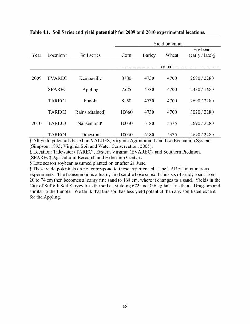
68

Table 4.1. Soil Series and yield potential† for 2009 and 2010 experimental locations.

Yield potential Year

Location‡

Soil series

Corn

Barley

Wheat

Soybean (early / late)§

--------------------------kg ha 1---------------------------

2009

EVAREC

Kempsville

8780

4730

4700

2690 / 2280

SPAREC

Appling

7525

4730

4700

2350 / 1680

TAREC1

Eunola

8150

4730

4700

2690 / 2280

TAREC2

Rains (drained)

10660

4730

4700

3020 / 2280

2010

TAREC3

Nansemond¶

10030

6180

5375

2690 / 2280

TAREC4

Dragston

10030

6180

5375

2690 / 2280

† All yield potentials based on VALUES, Virginia Agronomic Land Use Evaluation System (Simpson, 1993; Virginia Soil and Water Conservation, 2005). ‡ Location: Tidewater (TAREC), Eastern Virginia (EVAREC), and Southern Piedmont (SPAREC) Agricultural Research and Extension Centers. § Late season soybean assumed planted on or after 21 June. ¶ These yield potentials do not correspond to those experienced at the TAREC in numerous experiments. The Nansemond is a loamy find sand whose subsoil consists of sandy loam from 20 to 74 cm then becomes a loamy fine sand to 168 cm, where it changes to a sand. Yields in the City of Suffolk Soil Survey lists the soil as yielding 672 and 336 kg ha-1 less than a Dragston and similar to the Eunola. We think that this soil has less yield potential than any soil listed except for the Appling.

69

Table 4.2. Locations and soybean cultivars used at various planting dates in 2009.

Plan

ting

date

L

ocat

ion

C

ultiv

ar

1

2 3

4 5

6 E

VA

RE

C

A

G 4

907

27

May

R

8 Ju

ne R

B

23

Jun

e R

BW

----

‡

8

July

RBW

¶

15 J

uly

RBW

SP

AR

EC

AG

560

5

21 M

ay R

9

June

RB

22 J

une

RB

W

30

Jun

e B

W

9

July

RBW

15

Jul

y R

BW

TA

RE

C1

95

Y70

21

May

R†

4

June

RB

W

17

Jun

e R

BW

29 J

une

BW

7 Ju

ly R

BW

14 J

uly

RB

W

TA

RE

C2

A

G 4

907

21

May

R

2 Ju

ne R

B

11

Jun

e R

BW

29 J

une

BW

8 Ju

ly R

BW

§

14 J

uly

RBW

† So

ybea

n gr

own

afte

r rye

(R),

barl

ey (B

), an

d w

heat

(W) p

lant

ed (i

.e. f

our s

ubpl

ots

per s

mal

l gra

in).

‡ U

nabl

e to

pla

nt d

ue to

equ

ipm

ent m

alfu

nctio

n.

§ So

ybea

n gr

own

afte

r bar

ley

(B) o

r whe

at (W

) pla

nted

in s

ix s

ubpl

ots

inst

ead

of fo

ur.

¶ So

ybea

n gr

own

afte

r whe

at (W

) pla

nted

in e

ight

plo

ts p

er s

mal

l gra

in.

Table 4.3. Locations and soybean cultivars used at various planting dates in 2010.

Plan

ting

date

L

ocat

ion

C

ultiv

ars

1

2 3

4 5

6 7

8 9

TA

RE

C3

A

G 5

605

21 M

ay

28

May

3 Ju

ne

11

Jun

e

17 J

une

24

Jun

e

1 Ju

ly

8

July

16 J

uly

TA

RE

C4

A

G 4

907

22 M

ay

28

May

3 Ju

ne

11

Jun

e

17 J

une

23

Jun

e

1 Ju

ly

8

July

16 J

uly

70

Table 4.4. Treatment effects for soybean yield component measurements at four locations in 2009.

Yie

ld c

ompo

nent

mea

sure

men

t L

ocat

ion

Seed

yie

ld

(g m

-2)

Bio

mas

s (g

m-2

)

H

eigh

t pl

ant-1

Pl

ants

m

-2

Po

ds

m-2

Pods

pl

ant-1

Seed

m

-2

Se

ed

pod-1

Se

ed w

eigh

t (g

100

see

d-1)

P

value

E

VA

RE

C

.000

3

.004

9

<0.0

001

<0

.000

1

.004

7

<0.0

001

.0

031

.1

884

<0

.000

1 SP

AR

EC

<0

.000

1

<0.0

001

<0

.000

1

.000

4

<0.0

001

<0

.000

1

<0.0

001

.0

123

<0

.000

1 T

AR

EC

1

<0

.000

1

----

†

<0.0

001

<0

.000

1

.004

8

<0.0

001

<0

.000

1

<0.0

001

.0

105

TA

RE

C2

.287

7

.433

4

.227

0

.001

5

.348

6

<0.0

001

.2

639

.6

576

.6

254

† N

ot d

eter

min

ed.

71

Table 4.5. Treatment effects for soybean yield component measurements at two locations in 2010.

Yie

ld c

ompo

nent

mea

sure

men

t L

ocat

ion

Eff

ect

Seed

yie

ld

(g m

-2)

Bio

mas

s (g

m-1

)

H

eigh

t pl

ant-1

Pl

ants

m

-2

Po

ds

m-2

Pods

pl

ant-1

Seed

m

-2

Se

ed

pod-1

Se

ed w

eigh

t (g

100

see

d-1)

P value

T

AR

EC

3 W

G†

.549

1

.849

4

.039

4

.074

6

.661

9

.122

6

.411

0

.423

8

.266

1

PD‡

.425

2

.561

5

.003

6

.006

9

.376

0

.296

6

.269

5

.624

1

.007

4

WG

*PD

.5

201

.5

110

.4

530

.2

126

.6

518

.9

019

.3

084

.6

422

1.

0000

T

AR

EC

4 W

G

.035

4

.006

1

.242

4

<0.0

001

.0

052

.0

004

.0

117

.3

091

<0

.000

1

PD

.000

4

<0.0

001

<0

.000

1

<0.0

001

<0

.000

1

<0.0

001

<0

.000

1

.001

2

<0.0

001

W

G*P

D

.948

0

.955

5

.711

2

.900

9

.909

4

.967

3

.909

9

.627

9

.316

0 †

WG

, win

ter g

rain

. ‡

PD, p

lant

ing

date

.

72

Table 4.6. Seed yield, plant biomass, height, and yield components of soybean planted on different dates into a rye cover crop, or barley or wheat harvested for grain at EVAREC in 2009.

Planting date

27 May 8 June 23 June 8 July 15 July

Seed yield (g m-2)

Full-season 501.5a† 500.0a 403.3abcd 336.3bcd 275.3d

Barley-Soybean 497.0a 421.2abc 333.5bcd 290.5d

Wheat-Soybean 449.4ab 315.5cd 326.7cd

Biomass (g m-2)

Full-season 834a 890a 737abc 659abc 527c

Barley-Soybean 857a 721abc 621bc 531c

Wheat-Soybean 814ab 583c 597c

Height plant-1 (cm)

Full-season 74abcd 80ab 84a 72bcde 69cdef

Barley-Soybean 77abc 76abc 66def 61f

Wheat-Soybean 78abc 62f 63ef

Plants m-2

Full-season 24f 38def 44cde 66ab 50bcd

Barley-Soybean 26ef 39def 62abc 54abcd

Wheat-Soybean 51abcd 67a 68a

Pods m-2

Full-season 1803a

1675abc

1400abcd

1272bcd

984d

Barley-Soybean 1694ab

1497abc

1274cd

1006d

Wheat-Soybean 1550abc

1291cd

1301cd

73

Table 4.6. Continued.

Planting date

27 May 8 June 23 June 8 July 15 July

Pods plant-1

Full-season 80.3a 44.4c 37.1c 19.9e 20.6de

Barley-Soybean 66.0b 40.7c 20.9e 19.2e

Wheat-Soybean 32.7c 19.6e 19.2e

Seed m-2

Full-season 3527a 3622a 2891abcd 2513bcd 2076d

Barley-Soybean 3553a 3151abc 2529bcd 2210d

Wheat-Soybean 3252ab 2404cd 2478bcd

Seed pod-1

Full-season 2.0 2.2 2.1 2.0 2.1

Barley-Soybean 2.1 2.1 2.0 2.3

Wheat-Soybean 2.1 1.9 1.9

Seed weight (g 100 seed-1)

Full-season 14.2a 13.8bcd 14.0ab 13.5cde 13.3e

Barley-Soybean 14.0ab 13.4de 13.2e 13.2e

Wheat-Soybean 13.8abc 13.1e 13.2e

†Means within the same measurement followed by the same letter are not significantly different at p = 0.05 using Fisher’s Protected LSD.

74

Table 4.7. Seed yield, plant biomass, height, and yield components of soybean planted on different dates into a rye cover crop, or barley or wheat harvested for grain at SPAREC in 2009.

Planting date

21 May 9 June 22 June 30 June 9 July 15 July

Seed yield (g m-2)

Full-season 282.8ab† 349.7a 174.9bcde 113.1de 108.6de

Barley-Soybean 242.6bc 162.2cde 118.1de 104.2de 101.2e

Wheat-Soybean 187.5cd 122.0de 131.9de 119.1de

Biomass (g m-2)

Full-season 643ab 736a 374cd 261d 266d

Barley-Soybean 520bc 345d 270d 243d 246d

Wheat-Soybean 391cd 262d 274d 271d

Height plant-1 (cm)

Full-season 64a 56ab 49bc 37def 37def

Barley-Soybean 55b 44cd 35ef 37def 32f

Wheat-Soybean 42cde 37def 33f 32f

Plants m-2

Full-season 27ef 22f 32def 62abc 79a

Barley-Soybean 38cdef 39cdef 59abcd 57abcd 79a

Wheat-Soybean 49bcde 62abc 67ab 72ab

Pods m-2

Full-season 1374a 1548a 626bc 559bc 551bc

Barley-Soybean 866b 621bc 564bc 530bc 625bc

Wheat-Soybean 734bc 503c 578bc 592bc

75


Planting date


Pods plant-1

Full-season 52b 80a 27c 11c 7c

Barley-Soybean 25c 19c 11c 10c 8c

Wheat-Soybean 15c 8c 9c 8c

Seed m-2

Full-season 1911ab 2469a 1314bcd 948d 994d

Barley-Soybean 1702bc 1202cd 869d 862d 915d

Wheat-Soybean 1349bcd 934d 1084d 1029d

Seed pod-1

Full-season 1.4d 1.6bcd 2.1a 1.7bcd 1.8abc

Barley-Soybean 1.9ab 1.9ab 1.5cd 1.7bcd 1.5d

Wheat-Soybean 1.8abc 1.8abc 1.9ab 1.7bcd


Full-season 14.7a 14.2a 13.7ab 11.8def 11.1ef

Barley-Soybean 14.3a 13.5ab 13.5abc 12.2cdef 11.0f

Wheat-Soybean 13.8ab 12.8bcd 12.2cde 11.5ef


76

Table 4.8. Seed yield, plant biomass, height, and yield components of soybean planted on different dates into a rye cover crop, or barley or wheat harvested for grain at TAREC1 in 2009.

Planting date


Seed yield (g m-2)

Full-season 677.1a 584.8a 535.7abc 309.5cd 232.2d

Barley-Soybean 708.4a 651.8a 480.7abc 216.3d 203.9d

Wheat-Soybean 581.4ab 552.1ab 345.3bcd 181.6d 168.2d

Biomass (g m-2)

Full-season ----‡ ---- ---- ---- ---- ----

Barley-Soybean ---- ---- ---- ---- ---- ----

Wheat-Soybean ---- ---- ---- ---- ---- ----

Height plant-1 (cm)

Full-season 74fg 95bc 111a 92bcd 79defg

Barley-Soybean 81cdef 94bc 80def 90bcde 73fg

Wheat-Soybean 76efg 96ab 90bcde 73fg 65g

Plants m-2

Full-season 27fg 17g 45cde 65b 82a

Barley-Soybean 28efg 34def 36def 54bc 82a

Wheat-Soybean 25fg 48bcd 33def 64b 64b

Pods m-2

Full-season 2259a 1903ab 1812abc 1295bcd 1393bcd

Barley-Soybean 2232a 2205a 1690abc 1242bcd 1213bcd

Wheat-Soybean 1927ab 1713abc 1277bcd 1039cd 957d

77


Planting date


Pods plant-1

Full-season 93b 142a 51bcde 21de 17e

Barley-Soybean 81bc 66bcd 48bcde 25de 15e

Wheat-Soybean 95ab 39cde 43cde 16e 16e

Seed m-2

Full-season 4204a 3700ab 3394abc 2016cd 1548d

Barley-Soybean 4557a 4235a 3221abc 1393d 1341d

Wheat-Soybean 3731ab 3619ab 2276bcd 1191d 1159d

Seed pod-1

Full-season 1.86a 1.96a 1.85ab 1.51bc 1.12d

Barley-Soybean 2.06a 1.88a 1.91a 1.13d 1.06d

Wheat-Soybean 1.96a 2.01a 1.78ab 1.11d 1.19cd


Full-season 16.1a 15.8ab 15.6ab 15.5abcd 14.9de

Barley-Soybean 15.5abcd 15.4abcd 14.9cde 15.7abc 15.5abcd

Wheat-Soybean 15.5abcd 15.5abcd 15.2bcde 15.0cde 14.6e


‡Data not collected.

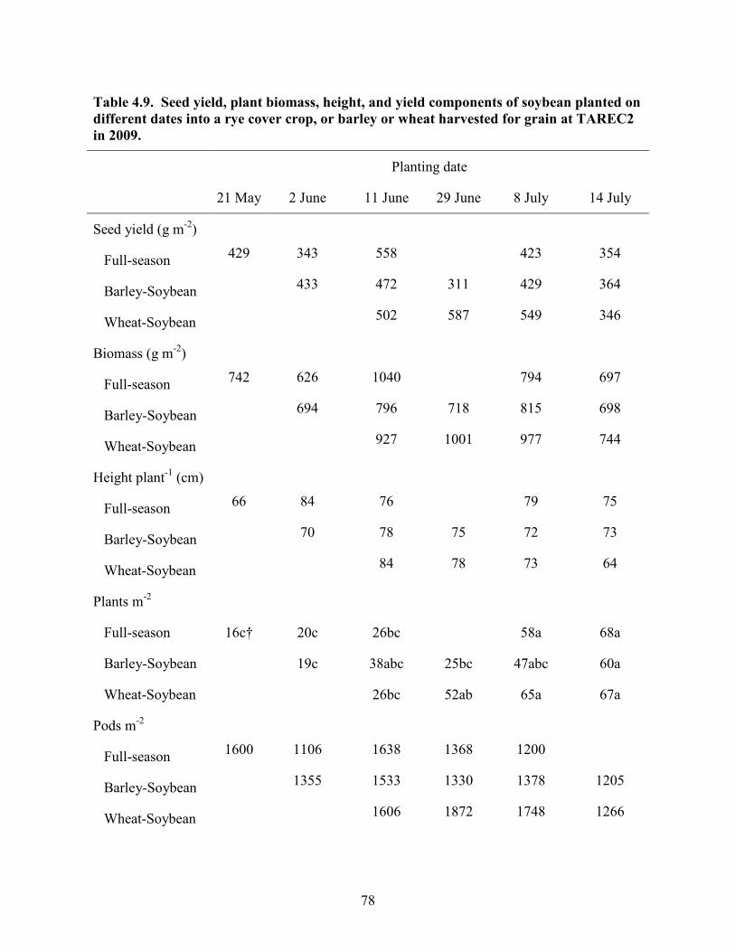
78

Table 4.9. Seed yield, plant biomass, height, and yield components of soybean planted on different dates into a rye cover crop, or barley or wheat harvested for grain at TAREC2 in 2009.

Planting date


Seed yield (g m-2)

Full-season 429 343 558 423 354

Barley-Soybean 433 472 311 429 364

Wheat-Soybean 502 587 549 346

Biomass (g m-2)

Full-season 742 626 1040 794 697

Barley-Soybean 694 796 718 815 698


Height plant-1 (cm)

Full-season 66 84 76 79 75

Barley-Soybean 70 78 75 72 73


Plants m-2

Full-season 16c† 20c 26bc 58a 68a

Barley-Soybean 19c 38abc 25bc 47abc 60a

Wheat-Soybean 26bc 52ab 65a 67a

Pods m-2

Full-season 1600 1106 1638 1368 1200

Barley-Soybean 1355 1533 1330 1378 1205

Wheat-Soybean 1606 1872 1748 1266

79


Planting date


Pods plant-1

Full-season 79ab 55abcd 67abc 25efg 18g

Barley-Soybean 78a 45cde 53bcd 30efg 21fg

Wheat-Soybean 61abc 39def 27efg 20g

Seed m-2

Full-season 2994 2406 3780 2904 2398

Barley-Soybean 2972 3205 2171 2944 2474

Wheat-Soybean 3491 4126 3753 2378

Seed pod-1

Full-season 2.2 2.2 2.3 2.1 2.0

Barley-Soybean 2.1 2.1 1.5 2.2 2.0

Wheat-Soybean 2.2 2.3 2.1 1.9


Full-season 14.3 14.3 14.7 14.6 14.7

Barley-Soybean 14.5 14.8 14.3 14.6 14.7

Wheat-Soybean 14.4 14.2 14.6 14.6


80

Table 4.10. Seed yield, plant biomass, height, and yield components of soybean planted on different dates into rye, barley,

wheat, or previous crop residue at TAREC3 in 2010.

Pl

antin

g da

te

21

May

28 M

ay

3

June

11 J

une

17

Jun

e

24 J

une

1

July

8 Ju

ly

16

Jul

y L

S m

eans

Se

ed y

ield

(g m

-2)

Fa

llow

-Soy

bean

16

5.4

19

5.1

20

4.7

14

4.2

18

7.1

20

9.1

24

5.8

16

8.1

21

8.8

19

3.1

R

ye-S

oybe

an

147.

4

167.

3

175.

5

145.

9

219.

2

174.

2

181.

4

188.

9

214.

2

179.

3

Bar

ley-

Soyb

ean

216.

1

282.

9

207.

8

194.

0

159.

8

138.

4

226.

5

164.

3

219.

2

201.

0

Whe

at-S

oybe

an

225.

2

145.

5

178.

7

214.

2

124.

0

166.

5

241.

5

175.

9

170.

3

182.

4

LS m

eans

18

8.5

19

7.7

19

1.6

17

4.6

17

2.5

17

2.1

22

3.8

17

4.3

20

5.6

Bio

mas

s (g

m-2

)

Fa

llow

-Soy

bean

41

9

482

48

7

340

45

3

495

54

3

385

53

8

460

R

ye-S

oybe

an

410

46

2

444

38

5

538

44

6

444

43

4

484

45

0

Bar

ley-

Soyb

ean

535

55

0

495

51

8

383

38

5

547

42

8

448

47

6

Whe

at-S

oybe

an

612

37

5

497

54

2

352

45

8

562

43

2

420

47

2

LS m

eans

49

4

467

48

1

446

43

2

446

52

4

420

47

2

81

Tab

le 4

.10.

Con

tinue

d.

Pl

antin

g da

te

21

May

28 M

ay

3

June

11 J

une

17

Jun

e

24 J

une

1

July

8 Ju

ly

16

Jul

y L

S m

eans

H

eigh

t pla

nt-1

Fa

llow

-Soy

bean

56

58

62

63

68

73

68

65

63

64

b

Rye

-Soy

bean

68

64

73

72

69

75

75

53

60

68

ab

B

arle

y-So

ybea

n

52

64

65

74

68

67

77

73

66

67

ab

W

heat

-Soy

bean

74

62

71

75

70

81

74

71

64

71

a

LS m

eans

62

c

62c

68

abc

71

ab

69

abc

74

a

73a

65

bc

63

c

Plan

t m-2

Fa

llow

-Soy

bean

45

45

37

32

38

39

35

39

82

43

R

ye-S

oybe

an

47

45

49

47

56

41

41

57

52

48

B

arle

y-So

ybea

n

51

33

35

51

33

30

45

41

56

42

W

heat

-Soy

bean

45

29

37

53

32

35

31

49

40

39

LS

mea

ns

47ab

38b

40

b

45b

40

b

36b

38

b

46ab

57a

82

Tab

le 4

.10.

Con

tinue

d.

Pl

antin

g da

te

21

May

28 M

ay

3

June

11 J

une

17

Jun

e

24 J

une

1

July

8 Ju

ly

16

Jul

y L

S m

eans

Po

ds m

-2

Fa

llow

-Soy

bean

76

4

1029

1035

724

86

7

888

11

18

72

0

1073

913

R

ye-S

oybe

an

877

88

6

936

77

4

1213

890

77

6

868

98

6

912

B

arle

y-So

ybea

n

11

80

11

99

11

74

83

9

780

78

9

1042

780

11

12

98

8

Whe

at-S

oybe

an

1163

775

11

35

10

85

75

7

963

87

6

881

90

2

976

LS

mea

ns

1070

1018

1014

996

97

2

904

88

3

855

81

2

Pods

pla

nt-1

Fa

llow

-Soy

bean

22

.0

25

.0

28

.0

32

.9

22

.0

30

.6

32

.2

20

.0

16

.6

26

.8

R

ye-S

oybe

an

21.2

22.0

20.4

17.3

21.6

23.0

19.3

17.3

20.3

21.4

Bar

ley-

Soyb

ean

24.4

37.5

33.5

16.5

24.2

31.7

23.6

22.7

23.3

27.4

Whe

at-S

oybe

an

26.8

26.2

35.0

21.6

26.1

29.9

34.8

20.1

61.3

30.9

LS m

eans

24

.7

31

.0

29

.8

22

.4

22

.8

34

.1

27

.6

19

.8

27

.4

83

Tab

le 4

.10.

Con

tinue

d.

P

lant

ing

date

21 M

ay

28

May

3 Ju

ne

11

Jun

e

17 J

une

24

Jun

e

1 Ju

ly

8

July

16 J

uly

LS

mea

ns

Seed

m-2

Fa

llow

-Soy

bean

17

13

18

31

20

97

13

95

17

97

21

17

23

15

14

62

19

33

18

51

R

ye-S

oybe

an

1463

1673

1802

1416

2183

1733

1728

1703

1937

1738

Bar

ley-

Soyb

ean

2298

2744

2157

1937

1533

1421

2209

1609

2101

2001

Whe

at-S

oybe

an

2497

1506

1919

2095

1306

1692

2527

1725

1569

1871

LS m

eans

19

93

19

39

19

94

17

11

17

05

17

41

21

95

16

25

18

85

Seed

pod

-1

Fa

llow

-Soy

bean

3.

03

1.

79

2.

03

1.

92

1.

99

2.

37

2.

07

2.

04

1.

81

2.

12

R

ye-S

oybe

an

1.67

1.94

1.92

1.85

1.81

1.96

2.25

1.94

1.98

1.92

Bar

ley-

Soyb

ean

1.98

2.76

1.80

2.40

1.94

1.85

2.11

2.04

1.93

2.09

Whe

at-S

oybe

an

2.11

2.02

1.66

1.09

1.77

1.77

2.41

2.02

1.84

1.95

LS m

eans

2.

20

2.

13

1.

85

2.

02

1.

88

1.

99

2.

21

2.

01

1.

89

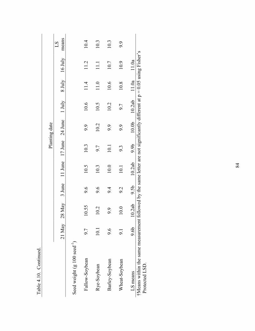
84

Tab

le 4

.10.

Con

tinue

d.

Plan

ting

date

21 M

ay

28

May

3 Ju

ne

11

Jun

e

17 J

une

24

Jun

e

1 Ju

ly

8

July

16 J

uly

LS

mea

ns

Seed

wei

ght (

g 10

0 se

ed-1

)

Fa

llow

-Soy

bean

9.

7

10.5

5

9.6

10

.5

10

.3

9.

9

10.6

11.4

11.2

10.4

Rye

-Soy

bean

10

.1

10

.2

9.

6

10.3

9.7

10

.2

10

.5

11

.0

11

.1

10

.3

B

arle

y-So

ybea

n

9.

6

9.9

9.

4

10.0

10.1

9.9

10

.2

10

.6

10

.7

10

.3

W

heat

-Soy

bean

9.

1

10.0

9.2

10

.1

9.

3

9.9

9.

7

10.8

10.9

9.9

LS

mea

ns

9.6b

10.2

ab

9.

5b

10

.2ab

9.9b

10.0

b

10.2

ab

11

.0a

11

.0a

†

Mea

ns w

ithin

the

sam

e m

easu

rem

ent f

ollo

wed

by

the

sam

e le

tter a

re n

ot s

igni

fica

ntly

dif

fere

nt a

t p =

0.0

5 us

ing

Fish

er’s

Pr

otec

ted

LSD

.

85

Table 4.11. Seed yield, plant biomass, height, and yield components of soybean planted on different dates into rye, barley,

wheat, or previous crop residue in 2010.

Pl

antin

g da

te

22

May

28 M

ay

3

June

11 J

une

17

Jun

e

23 J

une

1

July

8 Ju

ly

16

Jul

y L

S m

eans

Se

ed y

ield

(g m

-2)

Fa

llow

-Soy

bean

24

0.6

22

3.5

16

5.2

21

9.7

24

3.3

89

.0

12

8.4

19

7.1

16

1.6

18

5b†

R

ye-S

oybe

an

326.

2

244.

8

239.

6

213.

2

204.

2

255.

7

158.

6

184.

5

151.

7

220a

b

Bar

ley-

Soyb

ean

267.

7

319.

4

272.

0

273.

7

262.

5

204.

2

203.

9

192.

8

191.

3

243a

Whe

at-S

oybe

an

270.

7

242.

7

183.

1

233.

0

255.

1

196.

9

161.

1

151.

9

178.

5

208a

b

LS m

eans

27

6a

25

8ab

21

5bcd

e

235a

bcd

24

1abc

186c

de

16

3e

18

2de

17

1e

Bio

mas

s (g

m-2

)

Fallo

w-S

oybe

an

513

49

5

370

46

1

492

17

7

265

39

0

312

38

6b

R

ye-S

oybe

an

676

57

6

533

48

6

480

55

9

306

38

2

307

47

8a

B

arle

y-So

ybea

n

58

4

745

60

9

617

59

6

456

39

8

386

40

6

533a

Whe

at-S

oybe

an

591

55

9

423

54

8

583

40

2

301

31

6

374

45

5ab

LS

mea

ns

59

1a

59

4a

48

4ab

52

8a

53

8a

39

8bc

31

7c

36

8bc

35

0c

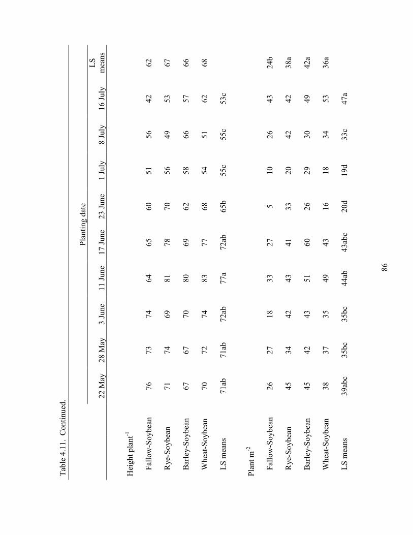
86

T

able

4.1

1. C

ontin

ued.

Pl

antin

g da

te

22

May

28 M

ay

3

June

11 J

une

17

Jun

e

23 J

une

1

July

8 Ju

ly

16

Jul

y L

S m

eans

H

eigh

t pla

nt-1

Fa

llow

-Soy

bean

76

73

74

64

65

60

51

56

42

62

R

ye-S

oybe

an

71

74

69

81

78

70

56

49

53

67

B

arle

y-So

ybea

n

67

67

70

80

69

62

58

66

57

66

W

heat

-Soy

bean

70

72

74

83

77

68

54

51

62

68

LS

mea

ns

71ab

71ab

72ab

77a

72

ab

65

b

55c

55

c

53c

Plan

t m-2

Fa

llow

-Soy

bean

26

27

18

33

27

5 10

26

43

24

b

Rye

-Soy

bean

45

34

42

43

41

33

20

42

42

38

a

Bar

ley-

Soyb

ean

45

42

43

51

60

26

29

30

49

42

a

Whe

at-S

oybe

an

38

37

35

49

43

16

18

34

53

36

a

LS m

eans

39

abc

35

bc

35

bc

44

ab

43

abc

20

d

19d

33

c

47a

87

Tab

le 4

.11.

Con

tinue

d.

Pl

antin

g da

te

22

May

28 M

ay

3

June

11 J

une

17

Jun

e

23 J

une

1

July

8 Ju

ly

16

Jul

y L

S m

eans

Po

ds m

-2

Fa

llow

-Soy

bean

97

5

924

73

0

905

96

1

291

44

6

745

62

7

734b

Rye

-Soy

bean

13

61

10

81

10

49

10

05

95

1

1105

553

72

7

563

93

3a

B

arle

y-So

ybea

n

11

02

13

29

11

53

12

80

11

75

88

8

749

71

9

757

10

17a

W

heat

-Soy

bean

11

73

10

73

88

3

1077

1196

780

55

4

567

65

2

884a

b

LS m

eans

11

53a

11

02a

95

4ab

10

66a

10

71a

76

6bc

57

6c

68

9c

65

0c

Pods

pla

nt-1

Fa

llow

-Soy

bean

43

.7

30

.1

40

.5

35

.7

41

.0

66

.0

47

.1

29

.6

16

.8

41

.0a

R

ye-S

oybe

an

32.2

30.7

24.2

21.9

23.8

38.4

29.8

17.5

14.8

25.5

b

Bar

ley-

Soyb

ean

28.0

31.6

30.9

27.1

23.4

45.7

27.9

25.1

17.0

27.3

b

Whe

at-S

oybe

an

29.7

35.0

27.4

23.5

30.0

50.6

32.8

16.7

14.5

28.0

b

LS m

eans

34

.3bc

27.2

bc

29

.8bc

27.6

bc

32

.1bc

48.6

a

35.7

b

23.2

cd

15

.3d

88

Tab

le 4

.11.

Con

tinue

d.

P

lant

ing

date

22 M

ay

28

May

3 Ju

ne

11

Jun

e

17 J

une

23

Jun

e

1 Ju

ly

8

July

16 J

uly

LS

mea

ns

Seed

m-2

Fa

llow

-Soy

bean

19

24

17

68

13

99

19

30

20

60

73

6

966

14

53

12

35

14

97b

R

ye-S

oybe

an

2611

1972

2132

1838

1924

2216

1201

1374

1126

1821

a

Bar

ley-

Soyb

ean

2139

2644

2438

2443

2450

1886

1606

1421

1448

2054

a

Whe

at-S

oybe

an

2287

1969

1621

2079

2337

2056

1232

944

13

53

17

91ab

LS m

eans

22

40a

20

88ab

1897

ab

20

72ab

2193

ab

17

24bc

1251

c

1360

c

1290

c

Seed

pod

-1

Fa

llow

-Soy

bean

1.

98

1.

85

1.

93

2.

18

2.

18

2.

39

2.

13

1.

95

1.

95

2.

06

R

ye-S

oybe

an

1.88

1.85

2.03

1.83

2.05

2.00

2.15

1.84

2.03

1.96

Bar

ley-

Soyb

ean

1.98

1.93

2.13

1.90

2.13

2.08

2.15

1.94

1.90

2.01

Whe

at-S

oybe

an

1.98

1.75

1.83

2.01

1.90

2.21

2.25

2.12

2.18

2.02

LS m

eans

1.

95cd

1.84

d

1.97

cd

1.

98cd

2.06

abc

2.

16ab

2.18

a

1.96

cd

2.

02bc

89

Tab

le 4

.11.

Con

tinue

d.

Plan

ting

date

22 M

ay

28

May

3 Ju

ne

11

Jun

e

17 J

une

23

Jun

e

1 Ju

ly

8

July

16 J

uly

LS

mea

ns

Seed

wei

ght (

g 10

0 se

ed-1

)

Fa

llow

-Soy

bean

12

.5

12

.6

11

.8

11

.5

11

.6

13

.0

13

.7

13

.6

13

.3

12

.6a

R

ye-S

oybe

an

12.5

12.6

11.2

11.4

10.6

11.5

13.3

13.5

13.5

12.2

b

Bar

ley-

Soyb

ean

12.5

12.1

11.2

11.3

10.7

10.8

12.7

13.5

13.2

12.0

b

Whe

at-S

oybe

an

12.0

12.3

11.2

11.2

10.9

11.0

13.1

13.0

13.2

12.0

b

LS m

eans

12

.4b

12

.4b

11

.3cd

11.4

cd

10

.9d

11

.6c

13

.2a

13

.4a

13

.3a

†

Mea

ns w

ithin

the

sam

e m

easu

rem

ent f

ollo

wed

by

the

sam

e le

tter a

re n

ot s

igni

fica

ntly

dif

fere

nt a

t p =

0.0

5 us

ing

Fish

er’s

Pr

otec

ted

LSD

.

90

Fig. 4.1. Influence of planting date and winter grain on full-season and double-cropped soybean yield† at EVAREC, SPAREC, TAREC1, and TAREC2 in 2009.

91


† Least squares means with standard error.

92

Fig. 4.2. Influence of planting date on full-season and double-cropped soybean yield at TAREC3 and TAREC4 in 2010.

93

Fig. 4.3. Maximum and minimum temperatures and rainfall† at EVAREC, SPAREC, and TAREC in 2009, and TAREC in 2010.

94


†TAREC rainfall does not include 50 mm of irrigation on 15 July 2009 and 25 mm on two occasions on 1 and 20 July 2010.

95

APPENDIX A

App

endi

x A

: Pr

oduc

tion

cost

s us

ed to

cal

cula

te n

et re

turn

s fo

r ful

l-se

ason

and

dou

ble-

crop

ped

soyb

ean

syst

ems

from

200

8-20

10.

Full-

Seas

on

Fallo

w-S

oybe

an

Fu

ll-Se

ason

R

ye-S

oybe

an

D

oubl

e-C

ropp

ed

Bar

ley-

Soyb

ean

D

oubl

e-C

ropp

ed

Whe

at-S

oybe

an

Pre-harvest variable costs

Seed

Sm

all G

rain

----

30.0

0

22.5

0

35.0

0

Soyb

ean

32

.00

32

.00

48

.00

48

.00

Fert

ilize

r

VA

RIE

S

VA

RIE

S

VA

RIE

S

VA

RIE

S Fe

rtili

zer A

pplic

atio

n

7.25

7.25

7.25

7.25

L

ime

(Pro

rate

d)

16

.25

16

.25

16

.25

16

.25

Pest

icid

es

28

.00

28

.00

49

.19

47

.94

Fuel

, Oil,

Lub

e

3.71

6.74

8.74

8.74

R

epai

rs

7.

44

12

.60

13

.16

13

.16

Pre-

Har

vest

Lab

or

2.

90

4.

93

6.

67

6.

67

Cro

p In

sura

nce

13

.36

13

.36

19

.26

24

.82

96

App

endi

x A

. Con

tinue

d.

Full-

Seas

on

Fallo

w-S

oybe

an

Fu

ll-Se

ason

R

ye-S

oybe

an

D

oubl

e-C

ropp

ed

Bar

ley-

Soyb

ean

D

oubl

e-C

ropp

ed

Whe

at-S

oybe

an

Harvest Variable Costs

Fuel

, Oil,

Lub

e

5.05

5.05

10.1

0

10.1

0 R

epai

rs

6.

26

6.

26

12

.52

12

.52

Har

vest

Lab

or

2.

61

2.

61

5.

08

5.

08

Hau

ling

8.

75

8.

75

30

.75

24

.00

Fixed Costs

Mac

hine

ry

29

.20

40

.60

60

.79

60

.79

Gen

eral

Ove

rhea

d

14.1

4

17.2

8

30.1

8

32.7

9

97

APPENDIX B

Appendix B. Annual, average, and median prices for soybean, barley, wheat, and corn across Virginia and at several delivery stations from 2006 to 2010. Appendix B1. Annual, average, and median prices of soybean, barley, wheat, and corn across Virginia, and at delivery stations in Petersburg and Tappahannock, Virginia, from 2006 to 2010.

Soybean

Barley

Wheat

Corn

$ / bushel

Virginia

2006

6.54

1.54

3.24

3.07

2007

11.40

2.76

5.78

4.39

2008

9.10

4.22

5.88

4.51

2009

9.40

2.37

4.07

3.66

2010

11.80

2.45

5.00

5.10

Average

9.65

3.33

4.79

4.15

Median

NA†

NA

NA

NA

Petersburg

2006

5.63

1.35

3.35

2.70

2007

8.15

2.11

5.87

3.91

2008

11.93

3.21

6.38

5.44

2009

9.95

2.04

4.00

4.09

2010

10.28

----

5.13

4.59

Average

9.19

2.18

4.95

4.15

Median

9.19

2.25

4.08

4.04

98

Appendix B1. Continued.

Tappahannock

2006

5.73

----

3.33

2.58

2007

8.32

2.62

5.57

3.83

2008

12.12

3.87

6.91

5.04

2009

10.11

2.70

3.67

3.90

2010

9.33

----

2.69

3.76

Average

9.12

2.18

4.43

3.82

Median

9.15

2.25

3.99

3.78

† NA, not applicable.

99

Appendix B2. Annual, average, and median prices for Chicago Mercantile Exchange July corn and estimated annual, average, and median prices for Osage Bio Energy barley at Hopewell and Tappahannock, Virginia, from 2006 to 2010.

Chicago Corn

Hopewell Barley†

Tappahannock Barley‡

$ / bushel 2006

2.87

2.29

2.04

2007

3.97

3.18

2.93

2008

5.57

4.45

4.20

2009

3.93

3.15

2.90

2010

4.48

3.58

3.33

Average

4.16

3.33

3.08

Median

3.99

3.19

2.92

† Hopewell barley prices are calculated as 20% of Chicago Mercantile Exchange July corn prices. ‡ Tappahannock barley prices are calculated as 20% of Chicago Mercantile Exchange July corn prices less a $.25 per bushel basis.

100

APPENDIX C

Appendix C: Full-Season, Double-Cropped Barley-Soybean, and Double-Cropped Wheat-Soybean Example Enterprise Budgets. Appendix C1: Full-Season Soybean Example Enterprise Budget

101

Appendix C2: Double-Cropped Barley-Soybean System Example Enterprise Budget

102

Appendix C3: Double-Cropped Wheat-Soybean System Example Enterprise Budget

Agronomic and Economic Comparison of Full-Season … committee members, Drs. David Holshouser, Wade...

Documents

Transcript of Agronomic and Economic Comparison of Full-Season … committee members, Drs. David Holshouser, Wade...