Instructions for use

Title Agricultural Remote Sensing by Multiple Sensors Mounted on an Unmanned Aerial Vehicle

Author(s) 杜, 蒙蒙

Citation 北海道大学. 博士(農学) 甲第13156号

Issue Date 2018-03-22

DOI 10.14943/doctoral.k13156

Doc URL http://hdl.handle.net/2115/70180

Type theses (doctoral)

File Information Du_Mengmeng.pdf

Hokkaido University Collection of Scholarly and Academic Papers : HUSCAP

Agricultural Remote Sensing by Multiple Sensors

Mounted on an Unmanned Aerial Vehicle

(無人飛行機に搭載した複数センサによる農業

リモートセンシング)

BY

杜 蒙蒙

DISSERTATION

Submitted to Division of Environmental Resources in

Graduate school of Agriculture, Hokkaido University, Sapporo, Japan,

in partial fulfillment of the requirements for the degree of

Doctor of Philosophy

March 2018

i

Table of Contents

Table of Contents ...................................................................................................................... i

Acknowledgement .................................................................................................................. iii

List of Figures ........................................................................................................................... v

List of Tables ........................................................................................................................ viii

Notations .................................................................................................................................. ix

Acronyms and Abbreviations ................................................................................................ xi

Chapter 1 Introduction ........................................................................................................ 1

1.1 Research Background ........................................................................................................... 1

1.1.1 Evolution of Agriculture ............................................................................................... 1

1.1.2 Precision Agriculture .................................................................................................... 3

1.1.3 Agricultural Remote Sensing ....................................................................................... 8

1.2 Research Objectives & Organization of Dissertation ...................................................... 14

Chapter 2 Conducting Topographic Survey Using UAV-LiDAR System .................... 16

2.1 Introduction ......................................................................................................................... 16

2.2 Research Platform and Equipment ................................................................................... 19

2.2.1 UAV Platform and Built-in Sensors .......................................................................... 19

2.2.2 LiDAR and Onboard Computer ................................................................................ 21

2.2.3 PPK-GPS modules and RTK-GPS modules ............................................................. 24

2.3 Methodology ........................................................................................................................ 27

2.3.1 Field Site and Experiment Description ..................................................................... 28

2.3.2 Acquisition of UAV-LiDAR System’s Attitude Information .................................. 29

2.3.3 Synchronizing LiDAR Distance Measurements with PPK-GPS Data ................... 35

2.3.4 Correcting LiDAR Distance Measurements and Calculating Ground Elevation . 37

2.4 Result and Discussion ......................................................................................................... 39

2.4.1 Accuracies of PPK-GPS Altitude and LiDAR Distance Measurements ................ 39

2.4.2 Validating UAV-LiDAR Based Topographic Surveying Accuracy ........................ 40

2.4.3 Visual Validation of UAV-LiDAR System Based Topographic Survey ................. 43

2.5 Conclusions .......................................................................................................................... 44

Chapter 3 Integrating Aerial Photogrammetric DSM with UAV-LiDAR System’s

Topographic Surveying Data ................................................................................................ 47

3.1 Introduction ......................................................................................................................... 47

3.2 Methodology ........................................................................................................................ 48

3.2.1 Interpolating Topographic Surveying Data .............................................................. 50

3.2.2 Generating Low-altitude Aerial Photogrammetric DSM ........................................ 57

ii

3.2.3 Integrating Aerial Photogrammetric DSM with UAV-LiDAR Data ...................... 60

3.3 Results and Discussion ........................................................................................................ 62

3.3.1 Evaluating Topographic Maps Based on Different Interpolating Methods .......... 63

3.3.2 Evaluating Accuracy of the Improved Topographic Map ...................................... 66

3.4 Validating Experiment on Large-scale Farmland ........................................................... 71

3.5 Conclusions .......................................................................................................................... 77

Chapter 4 Mapping within-Field Variations of Wheat Stalk Density ........................... 80

4.1 Introduction ......................................................................................................................... 80

4.2 Methodology ........................................................................................................................ 83

4.2.1 Field Site and Experiment Description ..................................................................... 84

4.2.2 Sampling of Stalk Density and Image Post-Processing............................................ 86

4.2.3 Calculating FGV and VCC ........................................................................................ 90

4.3 Results and Discussion ........................................................................................................ 95

4.3.1 Correlation Analysis between Sampled Stalk Density with FGV and VCC .......... 95

4.3.2 Mapping within-Field Spatial Variations of Stalk Density ..................................... 98

4.4 Experimental Validation of the Stalk Density Estimation Model................................. 102

4.5 Conclusion ......................................................................................................................... 106

Chapter 5 Multi-temporal Monitoring of Wheat Growth Status and Mapping within-

Field Variations of Wheat Yield ......................................................................................... 109

5.1 Introduction ....................................................................................................................... 109

5.2 Methodology ...................................................................................................................... 112

5.2.1 Field Site and Remote Sensing Images .................................................................... 112

5.2.2 Radiometric Normalization of Multi-temporal Remote Sensing Images ............. 116

5.2.3 Vegetation Indices of Remote Sensing Images ....................................................... 120

5.2.4 Sampling of Wheat Yield and Corresponding Vegetation Indices ....................... 124

5.3 Results and Discussion ...................................................................................................... 126

5.3.1 Multi-temporal Monitoring of Wheat Growth Status ........................................... 126

5.3.2 Mapping within-Field Variations of Wheat Yield .................................................. 131

5.3 Conclusion ......................................................................................................................... 133

Chapter 6 Summary ......................................................................................................... 135

References ............................................................................................................................. 139

List of Publications .............................................................................................................. 148

iii

Acknowledgement

Firstly, I would like to express my sincere gratitude to my supervisor Prof. Noboru

Noguchi with Research Faculty of Agriculture, Hokkaido Univ. for his valuable instruction

and advices during my study on agricultural remote sensing in Robotics and Vehicle

Laboratory. Civilian applications of unmanned aerial vehicle in recent year gained increasing

interests all over the world, and based on Prof. Noguchi’s insightful vision we opened a new

way of acquiring field information in a simple and autonomous fashion by using an

unmanned aerial vehicle as a platform. Using Prof. Noguchi’s knowledge in the domain of

precision agriculture for reference, we developed and studied on agricultural remote sensing

by integration of multiple sensors on board low-altitude unmanned aerial system. However,

the most difficult thing is to get started: we encountered tremendous hardships and obstacles

to operate the drone at first. It is the understanding, encouragement, and guidance from Prof.

Noguchi that pulled me through frustration and struggles in the first year of my study. I also

benefitted enormously from the discussion with Prof. Noguchi when we designed brand new

experiments using our hexa-copter, and the skills I learned from Prof. Noguchi will

accompany me throughout my lifetime.

I would also like to thank Prof. Kazunobu Ishii and Prof. Hiroshi Okamoto with Research

Faculty of Agriculture, Hokkaido Univ., for their assistance in conducting the experiments.

Without their help it would be impossible for me to acquire enough data and to finish my

dissertation. Days of experiments in Mackey of Australia, Memuro and Iwamiza of Japan

have witnessed our sweats and laughter, which will never fade in my memory. Prof. Ishii

appears to be informed, experienced, and sophisticated all the time. Anything went wrong

during experiments with electronic hardware, telemetry signal, and network configuration

and accessing, Prof. Ishii fixed it in no time. Prof. Okamoto’s preciseness and strictness

during the preparation of experiments before each field travel impressed me a lot, and I will

live by his example in my upcoming careers.

My appreciation also goes to Ms. Aoki and Ms. Namikawa, secretaries of Vehicle and

Robotics Laboratory, for taking good care of my research life over these three years so that I

could concentrate on my study without worrying about procedural regulations and official

businesses. I also would like to take this opportunity to thank Mr. Hiroyuki Sato and Mr.

Shinji Ichikawa with Field Science Center for Northern Biosphere, Experiment Farm,

Hokkaido Univ., as well as Mr. Tomonori Wada with Research Faculty of Agriculture,

iv

Hokkaido Univ., for shuttling between campus and farmlands with me. My UAV team

members, Miss Noriko Kobayashi, and Mr. Erdenebat Batzorig, together with other members

of Vehicle Robotics Lab., contributed a lot to collect field data, and I highly appreciate their

cooperation.

My Ph.D. study was supported by a joint scholarship program of CSC (China Scholarship

Council) and MEXT (Ministry of Education, Culture, Sports, Science and Technology),

Japan. I am forever grateful to CSC and MEXT for granting me this opportunity of studying

in Japan. Our experiments were funded by the R&D program of fundamental technology and

utilization of social big data by the National Institute of Information and Communications

Technology (NICT), Japan. Special acknowledgment also goes to Hokkaido Agricultural

Research Center and Hitachi Solutions Ltd. for assistance in preparing and conducting the

experiments.

My devotion to our beloved family is incomparable. The moment when I got injured and

frustrated during the experiment I found my fiancée Ms. Iwei Lu was there caring for me; the

moment when I remorse over the passing away of my grandmother and my uncle thousands

of miles away I found my parents were there consoling me; the moment when I rejoiced at

the acceptance of my research paper I found my sisters and my brother were there

encouraging me. This dissertation is dedicated to my dear nephew Yixuan, niece Zhiqin and

Zhiqian, who accompanied me to get over hard times and shared with me their innocent

laughter.

***Work out a flight path down-to-earth, and enjoy flying up high into the sky. ***

v

List of Figures

Fig.1. 1 Diagram of precision agriculture ............................................................................................... 5

Fig.1. 2 Access to multiple GNSS satellites ........................................................................................... 6

Fig.1. 3 Principle of DGPS ..................................................................................................................... 7

Fig.1. 4 Agricultural remote sensing in agriculture (based on a survey by Jacqueline K. and et al.) ..... 9

Fig.1. 5 Different platforms used in agricultural remote sensing ......................................................... 10

Fig.1. 6 Constitutional diagram of UAS (image courtesy: jDrones) ..................................................... 11

Fig.1. 7 Helicopter-style low-altitude UAV of Yammar (YH300) ....................................................... 13

Fig.1. 8 Fixed wing low-altitude UAV of Ag Eagle (RX60) ................................................................ 13

Fig.1. 9 Low-altitude multirotor UAV of EnRoute (CH940) ............................................................... 13

Fig.2. 1 Crop failure due to stagnant waters ......................................................................................... 16

Fig.2. 2 A small UAV used in this study .............................................................................................. 20

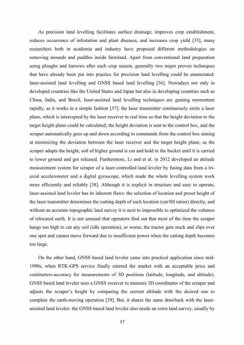
Fig.2. 3 PIXHAWK flight controller .................................................................................................... 21

Fig.2. 4 Airborne LiDAR application ................................................................................................... 22

Fig.2. 5 Laser beam divergence and spatial resolution ......................................................................... 23

Fig.2. 6 On board mini-computer.......................................................................................................... 24

Fig.2.7 RTK-GPS module and PPK-GPS module ................................................................................ 27

Fig.2. 8 Approach of generating topographic map ............................................................................... 27

Fig.2. 9 A harvested wheat field under study ....................................................................................... 28

Fig.2. 10 Rotation rates of gyroscope ................................................................................................... 32

Fig.2. 11 Raw accelerometer values ..................................................................................................... 33

Fig.2. 12 Pitch, roll and yaw values of the UAV-LiDAR system ......................................................... 34

Fig.2. 13 Simplified attitude estimation system of the UAV ................................................................ 35

Fig.2. 14 Raw data of PPK-GPS altitudes and LiDAR distance measurements ................................... 36

Fig.2. 15 Synchronized PPK-GPS altitudes and LiDAR distance measurements ................................ 36

Fig.2. 16 Corrected LiDAR distance measurements ............................................................................. 38

Fig.2. 17 Ground elevation of each surveying point ............................................................................. 38

Fig.2. 18 Accuracy of PPK-GPS coordiantes ....................................................................................... 39

Fig.2. 19 Accuracy of LiDAR distance measurements ......................................................................... 39

Fig.2. 20 Ground elevation of each surveying point showed in graduated symbols ............................. 40

Fig.2. 21 Distribution of validating samples ......................................................................................... 41

Fig.2. 22 Differences among validating samples’ ground elevation ..................................................... 42

Fig.2. 23 Field site of experiment for visual validation ........................................................................ 43

Fig.2. 24 Building bumps and hollows using a plough ......................................................................... 44

Fig.2. 25 Visual validation of spatial variations of within-field ground elevation ............................... 44

Fig.3. 1 (a) grid and (b) TIN based topographic modeling (Yih-ping Huang) ..................................... 50

Fig.3. 2 TIN model of the field under study ......................................................................................... 51

Fig.3. 3 Illustration of IDW method (by Esri) ...................................................................................... 52

Fig.3. 4 Interpolation result using IDW method ................................................................................... 53

Fig.3. 5 Interpolation result using spline method .................................................................................. 55

Fig.3. 6 Illustration of natural neighbor method (by Esri) .................................................................... 56

Fig.3. 7 Interpolation result using natural neighbor method ................................................................. 56

Fig.3. 8 Interpolation result using Kriging method ............................................................................... 57

vi

Fig.3. 9 Workflow of generating photogrammetric DSM..................................................................... 59

Fig.3. 10 The resulting photogrammetric DSM from aerial images ..................................................... 60

Fig.3. 11 Variations of RTK-GPS’s altitude and the corresponding DSM’s surface elevation data .... 60

Fig.3. 12 Improved spatial resolution of topographic surveying points ................................................ 62

Fig.3. 13 Distribution of RTK-GPS samples for evaluating interpolation models’ accuracy............... 64

Fig.3. 14 Variations of sampled ground elevation of RTK-GPS data and topographic maps .............. 65

Fig.3. 15 Variations of sampled ground elevation of RTK-GPS data and improved topographic maps

as well as the aerial photographic DSM ................................................................................................ 67

Fig.3. 16 Improved topographic maps using TIN interpolation method ............................................... 70

Fig.3. 17 Actual field condition of wheat (two days prior to harvesting) ............................................. 70

Fig.3. 18 Large-scale farmland used in the validating experiment ....................................................... 71

Fig.3. 19 The resulting aerial photogrammetric DSM .......................................................................... 72

Fig.3. 20 The resulting topographic map based on TIN interpolation method using UAV-LiDAR

system based topographic surveying data ............................................................................................. 73

Fig.3. 21 Spatial distribution of topographic surveying data in large-scale farmland .......................... 74

Fig.3. 22 The resulting topographic map by integrating aerial photogrammetric DSM and UAV-

LiDAR system based topographic surveying data ................................................................................ 75

Fig.3. 23 PPK-GPS samples’ spatial distribution ................................................................................. 76

Fig.4. 1 Wheat development stages (illustration of Nick Poole, FAR) ................................................. 81

Fig.4. 2 Proposed approach of using UAV-camera system to estimate wheat stalk density ................ 83

Fig.4. 3 Field site under study of estimating wheat stalk density ......................................................... 84

Fig.4. 4 ADC’s spectral response.......................................................................................................... 85

Fig.4. 5 Green-red-NIR false-color image of the field under study ...................................................... 86

Fig.4. 6 Matching keypoins for generating an Ortho-mosaic image ..................................................... 88

Fig.4. 7 Ortho-mosaic image of the wheat field shown in green-red-NIR false-color.......................... 89

Fig.4. 8 NDVI map ............................................................................................................................... 90

Fig.4. 9 Histogram of NDVI map ......................................................................................................... 93

Fig.4. 10 Image segmentation result using thresholding method .......................................................... 93

Fig.4. 11 Training dataset of SVM classification (in part) ................................................................... 94

Fig.4. 12 Classification result using SVM method ............................................................................... 95

Fig.4. 13 Regression models between sampled stalk densities with FGV ............................................ 96

Fig.4. 14 Regression models between sampled stalk densities with VCC ............................................ 97

Fig.4. 15 VCC samples’ spatial distribution used for generating stalk density map ............................ 98

Fig.4. 16 Resulting stalk density maps based on TIN, IDW, Kriging (upper images from left to right),

spline, and natural neighbor (bottom images from left to right) interpolation method ......................... 99

Fig.4. 17 Variation of estimated stalk densities based on different interpolation methods ................ 100

Fig.4. 18 Histogram of estimated stalk density map based on IDW interpolation method................. 102

Fig.4. 19 Vegetation classification result of wheat field for validating experiment ........................... 103

Fig.4. 20 Regression models between sampled stalk densities with VCC for validating experiment 104

Fig.4. 21 Estimated stalk density map for validating experiment ....................................................... 105

Fig.4. 22 Histogram of estimated stalk density map for validating experiment. ................................ 106

Fig.5. 1 Working principle of a combine harvester (Missotten, 1998) ............................................... 110

Fig.5. 2 Two neighboring wheat fields were studied planted with different winter wheat varieties .. 113

Fig.5. 3 Color change of wheat canopy shown by using satellite images in true color mode (Images

taken on June 1, 7, 15, and July 17, 2015 were demonstrated in sequence from left to right) ........... 113

vii

Fig.5. 4 Color change of wheat canopy was showed by using satellite images in standard false color

mode (Images taken on June 1, 7, 15, and July 17, 2015 were demonstrated in sequence from left to

right) .................................................................................................................................................... 114

Fig.5. 5 UAV’s flight path .................................................................................................................. 114

Fig.5. 6 UAV’s RGB images from heading stage to harvesting (the upper four images from left to

right were taken on June 2, 10, 19 and 25, and the lower four images from left to right were taken on

July 2, 10, 16 and 24, 2015) ................................................................................................................ 115

Fig.5. 7 Geo-referenced UAV’s Ortho-mosaic image overlaid upon satellite image ......................... 116

Fig.5. 8 Spatial distribution PIFs in satellite image (left) and UAV Ortho-mosaic image (right) ...... 118

Fig.5. 9 Typical spectral signature of different features (Saba Daneshgar) ........................................ 120

Fig.5. 10 Spatial distribution of vegetation indices............................................................................. 121

Fig.5. 11 Vegetation index maps based on UAV Ortho-mosaic images............................................. 125

Fig.5. 12 Close-shot photograph of the lodging spot in test wheat field............................................. 127

Fig.5. 13 Satellite image based vegetation indices ............................................................................. 129

Fig.5. 14 UAV Ortho-mosaic image based VDVI .............................................................................. 129

Fig.5. 15 Regression model between UAV images’ VDVI and satellite images’ VDVI ................... 130

Fig.5. 16 Regression model between UAV images’ VDVI and satellite images’ NDVI ................... 131

Fig.5. 17 Map of wheat yield (expressed as grain weight per square meter). ..................................... 132

Fig.5. 18 Histogram of wheat yield map ............................................................................................. 133

viii

List of Tables

Table 1. 1 Categories of UAVs ............................................................................................................. 12

Table 2. 1 Specifications of the UAV platform .................................................................................... 19

Table 2. 2 Specifications of LiDAR and onboard computer ................................................................. 24

Table 2. 3 Specifications of PPK-GPS modules ................................................................................... 25

Table 2. 4. Specifications of RTK-GPS module ................................................................................... 26

Table 2. 5 PPK-GPS coordinates (in part) ............................................................................................ 35

Table 3. 1 Flight plan and camera specifications .................................................................................. 58

Table 3. 2 Samples for evaluating accuracy of each interpolation method (in part) ............................. 63

Table 3. 3 Samples for evaluating accuracies of the aerial photogrammetric DSM and the improved

topographic maps (in part) .................................................................................................................... 68

Table 3. 4 Samples for evaluating accuracy of each interpolation method (in part) ............................. 75

Table 4. 1 Sampled stalk density and the corresponding FGV and VCC ............................................. 86

Table 4. 2 GCPs’ image space coordinates and geographic coordinates .............................................. 89

Table 4. 3 NDVI values of bare soil ..................................................................................................... 91

Table 4.4 Sampled stalk densities and estimated stalk densities based on different interpolation

models ................................................................................................................................................... 99

Table 4. 5 Sampled stalk densities and the corresponding VCC values of validating experiment ..... 102

Table 5. 1 PIFs’ pixel values of satellite images (taking blue band as an example) ........................... 117

Table 5. 2 Linear regression normalization models of satellites images ............................................ 118

Table 5.3 Linear regression normalization models of UAV images ................................................... 119

Table 5. 4 Satellite images based vegetation indices .......................................................................... 122

Table 5. 5 UAV ortho-mosaic images based VDVI ........................................................................... 123

Table 5. 6 Samples of wheat yield ...................................................................................................... 124

Table 5. 7 Time-varying NDVI and VDVI values calculated from satellite images .......................... 128

Table 5. 8 Time-varying VDVI values calculated from UAV’s Ortho-mosaic images ...................... 128

ix

Notations

a parameter of plane equation

b parameter of plane equation

c parameter of plane equation

eC constant variable of motor

cm centimeter

d raw LiDAR distance measurement

corrd

corrected LiDAR distance measurement

di distance of each measured point to the interpolation point

e ground elevation of surveying point

eRTKi ground elevation of and the RTK-GPS data

𝑒𝑈𝐴𝑉𝑖 ground elevation of the UAV-LiDAR system data

g gram

gx acceleration components in x axial from the accelerometer

gy acceleration components in y axial from the accelerometer

gz acceleration components in z axial from the accelerometer

hfix height difference between PPK-GPS rover antenna and LiDAR device

hppkgps altitude of PPK-GPS

Hz Hertz

I DC current through each motor

kg kilogram

Ko modified Bessel function

m meter

𝑚𝑥 magnetic intensity components in x axial

𝑚𝑦 magnetic intensity components in y axial

𝑚𝑧 magnetic intensity components in z axial

mrad milliradians

n rotational speed of each motor

Nt the total number of pixels within a unit area

Nv the number of pixels that are classified as vegetation

nidw the number of measured points included in the IDW model

nspl The number of measured points included in the spline model

nm nanometer

p power parameter of IDW model

R equivalent resistance of each motor’s coil

R(di) regularized algorithm’s coefficient

T(x, y) regularized algorithm’s coefficient

U voltage imposed upon each motor

V voltage

W watt

wi weighting factor of each measured point

x

ωx raw rotation rates of x axial from the gyroscope

ωy raw rotation rates of y axial from the gyroscope

ωz raw rotation rates of z axial from the gyroscope

x easting coordinate of each interpolation point

y northing coordinate of each interpolation point

z elevation coordinate of each interpolation point

z(x, y) estimated ground elevation of the interpolation point

z(xi, yi) measured point’s ground elevation

xi easting coordinate of each measured point

yi northing coordinate of each measured point

zi elevation coordinate of each measured point

magnetic flux of each motor’s coil

θ pitch

θacce

calculated pitch from accelerometer

θgyro

calculated pitch from gyroscope

ϕ roll

ϕacce calculated roll from accelerometer

ϕgyro calculated roll from gyroscope

ψ yaw

ψgyro

calculated yaw of UAV platform from gyroscope

ψmagn

calculated yaw from magnetometer,

ρNIR spectral reflectance of NIR waveband of the remote sensing data

ρred spectral reflectance of red waveband of the remote sensing data

xi

Acronyms and Abbreviations

ADC Agricultural Digital Camera

BC Before Christ

CMOS Complementary Metal-Oxide-Semiconductor

DC Direct Current

Dr. Doctor

DGPS Differential Global Positioning System

DSM Digital Surface Model

ExG Excessive Greenness

FGV Fractional Green Vegetation

GCP Ground Control Point

GCS Ground Control Station

GIS Geographic Information System

GLONASS GLObalnaya NAvigatsionnaya Sputnikovaya Sistema

GNSS Global Navigation Satellite System

GPS Global Positioning System

GRRI Green-Red Ratio Index

GS Growth Stage

HALE High-Altitude Long-Endurance

HTOL Horizontal Take-Off and Landing

IDW Inverse Distance Weighting

IMU Inertial Measurement Unit

IoT Internet of Things

IRNSS Indian Regional Navigation Satellite System

K Potassium

LiDAR Light Detection and Ranging

LiPo Lithium-Polymer

LOOCV Leave-One-Out Cross -Validation

MALE Medium-Altitude Long-Endurance

MAV Micro Aerial Vehicle

MEMS Micro-Electronic Magnetic System

N Nitrogen

NDVI Normalized Differential Vegetation Index

NGBDI Normalized Green-Blue Difference Index

NGRDI Normalized Green-Red Difference Index

NIR Near Infrared

P Phosphorus

PAs Pilotless Aircrafts

pH potential of Hydrogen

PIF Pseudo-Invariant Feature

PPK-GPS Post Processing Kinematic Global Positioning System

xii

QZSS Quasi-Zenith Satellite System

RGB Red-Green-Blue

RMSE Root Mean Square Error

RPAs Remotely Piloted Aircrafts

RPVs Remotely Piloted Vehicles

RS Remote Sensing

RTK-GPS Real Time Kinematic Global Positioning System

SfM Structure from Motion

SSCM Site-Specific Crop Management

SVM Support Vector Machine

TIN Triangulated Irregular Network

VTOL Vertical Take-off and Landing

VRS Virtual Reference Station

UAS Unmanned Aircraft System

UAV Unmanned Aerial Vehicle

USAF United State Air Force

USB Universal Serial Bus

UTM Universal Transverse Mercator

VCC Vertical Canopy Coverage

VDVI Visible-Band Difference Vegetation Index

WGS World Geodetic System

3D Three Dimensional

1

Chapter 1 Introduction

1.1 Research Background

1.1.1 Evolution of Agriculture

As the rapidly changing world keeps gaining momentum in respect of almost every

aspect of human life towards the direction of automation and intellectualization, agriculture,

which has always been the cornerstone of economic and social development both regionally

as well as globally in human civilizations, is also transforming itself into a high-level

scientific industry. Farming originated and evolved independently in many regions all over

the world, yet either the agricultural total output or the unit output stagnated for tens and

hundreds of centuries. Meanwhile, farming-engaged population kept increasing due to the

lack of efficient equipment, high-quality plant seeds, scientific agronomic methodologies,

and etc. Along with the global growth of population and social developments in human

civilization, agriculture industry has also experienced several major transformations: from

subsistence agriculture to commercialized agriculture, intensive agriculture, industrial

agriculture, and eventually the precision agriculture.

Subsistence agriculture refers to farming systems that depend on manpower as well as

animal power, by using hand tools and simple instruments to conduct agricultural production

activities in ancient times. Mainly for self-sufficient and self-contained purpose under natural

economic circumstances, subsistence farming enjoys the advantages of low energy

consumption and non-pollution but also has to suffer from low-yield or worse: total crop

failure in case of occurrence of natural disaster. Throughout the history of human civilization,

famine, a widespread scarcity of food, was closely associated with each social change and

reformation. The first famine in history was recorded 441 BC in ancient Rome, and in

Somalia during 2011-2012 the death toll of famine was estimated up to 285,000, caused by

2011 East Africa drought [1]. In order to combat famine in respect to both frequency and

severity, implementation of improved farming techniques and farming models to increase

crop yield has been witnessed all over the globe.

Between the 16th and 17th century in western countries and at the beginning of the 20th

century in oriental counties commercialization of agriculture emerged as feudal system fell

apart, and farmers began to possess their own farmland as private property. Thereafter

2

prosperous farmers turned themselves into capitalist landowners and they strived to improve

crop yields not merely for subsistence needs but for making a fortune by selling the surplus

crops to areas that demanded that product. More and more farmlands were transferred and

consolidated in the following years to certain distinguished individuals or corporations. As a

result, surpluses of agricultural production were by and large guaranteed. The eagerness for

profit was insatiable, and the power of capitals was infinite in promoting agricultural

development. To furthermore increase crop yields, innumerable agricultural researches were

initiated and experimental achievements on plants, soil, water, and all other crop related

topics emerged on after another. By the year of 1642, Dr. Jan Baptist van Helmont conducted

the famous 5-year willow experiment. Based on quantitative analysis, Dr. Helmont tested

whether plants obtain their mass from soil and he concluded that the gain mass of wood,

barks, and roots arose out of water only [2]. From then on, between the 17th and 18th

centuries knowledge on the mineral nutrition of plants widely disseminated owing to several

European naturalists. In 1727 Stephen Hales published experiment results on the nature of

transpiration: the transport of water and solutes in plants [3]. By the 1840s, Professor Justus

Freiherr Von Liebig, the pioneer of the agricultural chemistry and the “father of the fertilizer

industry” investigated on indispensable mineral salts including nitrogen (N), phosphorus (P),

and potassium (K) and concluded that N, P, and K, among other mineral elements are

essential to plant growth. Besides, Professor Liebig put forward the “Law of the Minimum”,

arguing that plant growth relies on the supply of the scarcest mineral nutrition that is

available to the plants [4]. The impact of “Law of the Minimum” on the agriculture industry

has been far reaching. Professor Liebig himself advocated the agricultural application of

nitrogen fertilizer to solve the problem of food availability, which fundamentally enlarged

agricultural activity into a capitalized industry on an unprecedented scale.

The development of agricultural techniques has been through zigzagging process. It was

not until the 1770s when the industrial revolution brought steam-powered machines into not

only factories but also farmlands that intensive farming on large scale came into realization.

However, as the old cliché goes that development of science and technology is always a

double-edged sword: the advent of efficient agricultural machinery made it possible to

produce adequate food for feeding more population, and global population boomed up to

about 800 million for the first time by the end of 18th century after the securing of food

production through massive agricultural mechanization [5], which in turn asked for more

provision of food and biomass resources as industrial raw materials. Urgent food demand

3

further stimulated scientists and researchers to discover outstanding plant breeds suitable for

intensive agriculture; to develop new plant varieties with specific capabilities such as drought

tolerance, lodging-resistance, and high yields; to introduce new farming technology including

man-made drainage systems, pesticides and herbicides, and synthetic fertilizers, etc. The

invention of ammonia from nitrogen gas (N2) and hydrogen gas (H2) by Fritz Haber in

collaboration with Carl Bosch in the 1910s fundamentally changed agriculture industry

globally. The Haber–Bosch process of artificially synthesizing ammonia is still mainly used

to produce nitrogen fertilizer today, accounting to 450 million tones anhydrous ammonia,

ammonium nitrate, and urea per year [6]. In combination of pesticides application and

adaptation of high-power agricultural machinery, massive use of synthetic fertilizers

improved productivity of agricultural land dramatically through intensive farming techniques

with higher levels of input and for higher levels of output per unit area of farmland.

Nowadays agricultures in most areas across the globe are intensive in one or more

respects: capital, labor, machinery, fertilizer, and agricultural chemicals. As investments in

intensive agriculture rely on industrial methods heavily, it is also referred to as industrial

agriculture. At the meantime gene-modified breeds as well as hybridization crops also

obtained rapid popularization. Around the 2010s breeding scientist Longping Yuan

announced the success of a new strain of hybrid rice that was reported to produce 13.9 tons of

rice per hectare [7], when the world population exceeded 6.9 billion [8]. In order to feed such

a large number of mouths and to swipe out starvation in a global context, updating

methodologies and equipment are introducing into intensive agriculture to cope with such

issues like the unbalance of agricultural ecology: the abuse of agricultural chemicals,

decreasing underground water level, soil compaction and erosion, land degradation and

dissertation, etc. [9]. Using automated agricultural machinery and variable-rate technology in

precision agriculture or site-specific crop management (SSCM) emerged as the times

required in recent years, which enables each farmer to be able to feed 265 people on average,

comparing with each farmer feeding 26 people on average in the 1960s [10].

1.1.2 Precision Agriculture

Precision agriculture improves upon the advantageous techniques used in intensive

agriculture, whilst reduces the negative impacts on agricultural ecology for a low-input, high-

efficiency, and sustainable agriculture [11]. Precision agriculture could also be called as

ecological agriculture or eco-agriculture to some extent, as its prime objective is to construct

4

a decision supporting system by acquiring site-specific field information and responding to

the within-field spatial variability [12]. The ultimate goal of precision agriculture is to build a

sustainable agriculture by protecting arable land from degradation and pollution, and utilize

agricultural inputs in a more efficient way without compromising the high-productivity of the

present intensive agriculture system. The demand of precision agriculture rose after the

completion of agricultural mechanization in well developed countries in the early 1980s,

when farmers intended to maximize profit by dividing vast farmlands into smaller

management zones and varying treatments of fertilizers and/or agricultural chemicals in

response to the variability of each specific management zone [13]. Meanwhile researchers as

well as policy-makers became concerned about environmental issues like N leaching, water

pollution, and etc. [14]-[16].

The concept of precision agriculture was brought out by researchers at the University of

Minnesota in 1985, designing variable-rate lime input experiments for improving soil’s pH

(potential of hydrogen) value within a farmland [17]. Thereafter, the importance and

profitability of precision agriculture got universally acknowledged, many researchers all

around the world initiated precision agriculture related projects including sensors, automated

agricultural machinery, variable-rate agricultural implements, and etc. In 1989 Wagner and

Schrock installed a pivoted auger grain flow sensor on a commercial combine harvester to

determine within-field yield variations of wheat, so that general information on field

productivity could be obtained [18]. In 1999 Yule and et al. developed a differential global

positioning system (DGPS) based data acquisition system equipped on a tractor to map

within-field variability of topology and soil moisture content, so that areas that needs

remedial operations could be identified [19]. In 1999 Tian and et al. developed an intelligent

sensing and precision spraying system based on machine vision technology to estimate weed

density and size, so that herbicide application could be reduced by realizing site-specific

weed control [20]. In 2001 Hummel et al. developed a near infrared (NIR) soil sensor to

measure organic matters in soil and surface as well as subsurface soil’s moisture contents for

documenting the spatial variability of soil parameters [21]. In 2001 Noguchi et al. developed

a robot tractor based on RTK-GPS (Real Time Kinematic Global Positioning System),

gyroscope, and IMU (Inertial Measurement Unit) [22], which could conduct various kinds of

field operations with acceptable accuracy. From then on vehicle and robotics laboratory in

Hokkaido University developed a dual robot tractors system in master-slave fashion, and

multi-robot tractors system operating in collaboration with each other to further improve

5

working efficiency. Ever since the beginning of 21st century, numerous sensors are being

launched into agricultural market: handheld devices, equipment onboard ground vehicles,

airborne instruments, and satellite sensors have greatly enriched the means of acquiring field

information. In essence, the progress of precision agriculture has been closely linked to such

technologies including agricultural mechanization and automation, GPS, GIS (Geographic

Information System), IoT (Internet of Things) techniques, sensors, variable-rate applicators,

remote sensing techniques, and etc., depicted in Fig.1. 1.

Fig.1. 1 Diagram of precision agriculture

As the massive production capability and reliability of integrated circuit products, or

microchips, have been validated by market since the 1960s, numerous kinds of industrial

sensors that are capable of collecting and processing instantaneous information were

developed, which marked the advert of information era. GPS is deemed as one of the most

successfully commercialized industrial technologies thanks largely to the extensive use of the

miniaturized and economical integrated circuit products, which consists of three main

segments: the space segment, the ground control segment, and the user segment. In a sense it

is like that each point on or nearby the planet has been virtually mapped and attached with a

unique coordinate, and all what the user needs is a GPS receiver to “estimate” one’s location

(coordinates) on the map based on trilateration method by measuring distance between GPS

receiver and GPS satellites [23].

The technical terminology of GNSS (Global Navigation Satellite System) is nowadays

more preferable to GPS by researchers, which is a generic term including several satellite

Variable-Rate Application

Land Preparation Crop Management Precision Harvesting ...

GIS Processing

Geo-referencing Mapping

Field Data Acquisition

Soil Condition

Water Stress Crop Growth

Status Yield

Variations ...

6

navigation and positioning systems providing global services. GNSS mainly comprises the

most widely used GPS of the United States of America, GLONASS (GLObalnaya

NAvigatsionnaya Sputnikovaya Sistema) of Russia, Beidou of China, GALILEO of European

Union, and each of them provides global positioning services at different levels of accuracy.

It also includes QZSS (Quasi-Zenith Satellite System) of Japan as well as IRNSS (Indian

Regional Navigation Satellite System) of India which provides regional positioning services

to some extent. Theoretically it needs at least four GNSS satellites and each of them forms an

unobstructed line of sight to a GNSS receiver in order to acquire a “fixed” 3D (three

dimensional) coordinates. However, more than four GNSS satellites are usually included

simultaneously into different navigation and positioning algorithms for higher accuracy, as

the extra cost of superfluous access to GNSS satellites from multiple systems than to a single

system is next to negligible. Fig.1. 2 showed an easy access to multiple GNSS satellites

using a smart phone in northern China on 3 October 2017, from which we can see that 24

GNSS satellites in total were visible by that time: 9 GPS satellites, 6 GLONASS satellites,

and 9 Beidou satellites, respectively.

Fig.1. 2 Access to multiple GNSS satellites

Yet the inevitable problem of low positioning accuracy (less than five meters

horizontally) resides with GNSS standalone positioning mode, due to clock precision,

ionospheric disturbance, and etc. Thus, different augmentation systems were created to

enhance positioning accuracy, integrity, and availability. DGPS improves GNSS positioning

7

accuracy up to about one meter, using a network of ground reference stations which

continuously broadcast the difference of distance between the known fixed positions and the

estimated positions indicated by the GNSS positioning algorithm. Subsequently, GNSS rover

rectifies each estimated pseudo-range between GNSS receiver and GNSS satellites according

to the correction information from base station, shown as Fig.1. 3. Basically RTK-GPS works

in the same manner as that of the DGPS, providing two to five centimeters accuracy; the only

difference is that RTK-GPS rover receives correction signal of carrier phase information from

base station instead of pseudo-range measurements. Centimeter-level accuracy as it is, RTK-

GPS requires a stable data link either via the radio signal or cellular network between the

GNSS rover and the base station. On the other hand, PPK-GPS (Post Processing Kinematic

Global Positioning System) processes the positioning information that is saved on board the

GNSS receivers after each operation. Similar to RTK-GPS, one GNSS receiver remains

stationary as a ground base station at a known position, whilst the other GNSS receiver that

“observes” the same combination of GNSS satellites (usually within twenty kilometers from

the ground base station) works as a rover receiver. However, when compared with RTK-GPS,

PPK-GPS provides a more precise relative positioning result as it traces both backward and

forward through the carrier phase data of these two GNSS receivers multiple times.

Nonetheless, the absolute positioning accuracy of PPK-GPS relates to the accuracy of the

“known” position of the ground base station, which is usually acquired by using a RTK-GPS

module or estimated from hour-long measurements of standalone GNSS positioning.

Fig.1. 3 Principle of DGPS

The utilization of global positioning services based on GNSS technology has profound

impact on the implementation of precision agriculture, which tagged each field sample’s

attribute value (soil condition, water stress, crop growth status, yield variation, and etc.) with

8

an accurate spatial coordinates – a process called geo-referencing or geo-coding. The

realization of processing these geo-referenced attribute values in GIS environment improved

field sampling efficiency and spatial accuracy at an unprecedented level, as GIS applications

are effective tools that enable researchers to visualize, edit, integrate, and analyze spatial-

temporal information in a digitalized fashion [24]. It is also worth mentioning that GIS

applications are capable of relating spatial-temporal information from different sources that is

geo-coded by using GNSS devices or geo-referenced by measuring GCPs’ (Ground

Controlling Point) geographical coordinates afterwards. GNSS based autonomous navigation

of agricultural machinery, i.e., tractors, transplanters, combine harvester, chemical spring

airplanes and drone, and etc., have been breaking new grounds in precision agriculture

domain. The mobile platform that not only knows where it is but also is aware of what it is

about to do: changing advancing velocity, making a turn, controlling attached applicators

according to a prescription map, and etc. Agricultural machinery equipped with GNSS

receiver also greatly improves logistical efficiency, as the display of real-time feedback of

vehicle’s position in GIS applications provides plentiful information for decision-making

relating to operation scheduling, path planning, shuttle truck arrangement. With the aid of

accurate GNSS navigation and positioning techniques and the powerful GIS data

management capabilities, we have good reason to believe that provision of adequate food,

preserving agricultural ecology, and guaranteeing industrial profit would be brought into

equilibrium in the future precision agriculture.

1.1.3 Agricultural Remote Sensing

In precision agriculture industry, information is king. The abundancy, frequency, as well

as accuracy of the acquired field information influence decision-makers greatly on

determining the appropriacy of each SSCM operation. The means of obtaining field

information are various. Primitively field survey by experienced farmers was used for the last

thousand years, in which visual inspection of stalk density, leaf area and pigment, number of

pests, and etc., acted as a sole information source. Not so long ago until mineral nutritious

elements were distinguished inside plant tissues that precise laboratory experiments came

into realization by taking samples from the field. Later on handheld devices are included into

field sampling operation, which mainly take advantage of spectroscopic technologies.

However, either it should be visual inspection or instrumental sampling in the field, data

collection can be enormously time consuming for the current large-scale farming. Moreover,

9

it is sometimes reported that the collected field information can be very deceptive when

samples are scare or partially focused in featured regions.

Remote sensing is the science and art of obtaining information about an object, area, or

phenomenon through the analysis of data acquired by a device without making physical

contact with the object, area, or phenomenon under investigation [25], which has been

successfully used as an effective and accurate means of collecting field information from the

farmland-level, to the regional level and global level. On the basis of different types of

remote sensing platforms carrying onboard sensors, agricultural remote sensing could

generally be categorized into satellite remote sensing, aerial remote sensing and near-ground

remote sensing. According to a survey conducted by Jacqueline and et al., at Purdue

University of crop input dealers and their use of precision technology, up to 39.2% of the

respondents used satellite or aerial remote sensing data for precision agriculture. The

increasing trend of monitoring crop growth status from remote sensing imagery is now being

accelerated by the easy access of civilian UAVs (Unmanned Aerial Vehicle).

Fig.1. 4 Agricultural remote sensing in agriculture (based on a survey by Jacqueline K. and et al.)

Traditionally, multi-spectral satellite imagery has been successfully used to detect

vegetation coverage, monitor crop growth status, and estimate crop yield, etc., in large scale

[26], [27]. Through quantitative analysis of digitalized numbers of different bands of satellite

images, or more often, of various kinds of vegetation indices calculated from the reflectance

or radiance of specific bands, regression models could be built between remote sensing data

% o

f re

spond

ents

10

and ground truths. However, low spatial resolution, long revisiting-period as well as

atmospheric effects, or weather interference, are known as inherent flaws of such kind of

multi-spectral satellite imagery used in precision agriculture domain. On the other hand,

aerial remote sensing using airplanes has been introduced into medium-scale agricultural

applications as a supplementary method and often carried out as one-time operations since

the 1950s [28]. Whilst near-ground remote sensing is often referred to as frame or pillar

based applications and sensing systems that are installed on agricultural vehicles in the past,

and recently the cutting edge application of small fixed-and/or rotary-wing drones or UAVs

used in small-scale and experimental fields, with various kinds of commercial RGB cameras,

multi-spectral cameras, and laser scanners mounted upon, shown in Fig.1. 5.

Fig.1. 5 Different platforms used in agricultural remote sensing

According to the definition of Federal Aviation Administration and the United State Air

Force (USAF), UAV refers to an aircraft that is operated without the direct human

intervention from within or on the aircraft, can fly autonomously or be piloted remotely, uses

aerodynamic forces to provide vehicle lift, can be expendable or recoverable, and can carry a

lethal or nonlethal payload. UAVs have also been called drones, RPVs (Remotely Piloted

Vehicles), RPAs (Remotely Piloted Aircrafts), PAs (Pilotless Aircrafts), and other terms over

the years depending upon their specific working scenarios. Current developments in UAVs

trace their beginnings to World War One, and the application of modern UAVs emerged in

11

late 1950s in such manners that the pilot has real-time remote monitoring and controlling of

the aircraft through command link and telemetry systems, in the development of unmanned

aerial reconnaissance projects initiated by the USAF. Meanwhile, applications of UAV for

non-military purposes was long time in its infancy until 2010s, when the multi-copter UAVs

related industries were promoted as new stimulus for booming economy by several countries

including China, the USA, Germany, and other governments. By then, the most intense use of

commercial UAVs took place in Japan, where vertical take-off and landing (VTOL)

helicopter-style UAVs are extensively operated under the jurisdiction of the Ministry of

Agriculture, Forestry and Fisheries for chemical spraying. Nowadays civilian UAVs come in

various kinds of shapes and sizes with widespread applications extending from professional

topographic surveying and recreational aerial photography, to monitoring disaster site, data

collection for precision agriculture, logistics, etc., due to the advantages of low cost,

versatility, good maneuverability and efficiency.

Fig.1. 6 Constitutional diagram of UAS (image courtesy: jDrones)

Furthermore, the conception of UAS (Unmanned Aircraft System) was recently put

forward, shown in Fig.1. 6, which refers to an integrated system usually compromised of the

unmanned aircraft, onboard navigational and controlling unit, data link system, payload,

peripheral equipment, and a GCS (Ground Control Station). The on-board navigational and

controlling unit usually includes the micro-computer, battery managing system, GNSS unit,

MEMS (Micro-Electronic Magnetic System) unit, gyroscope, barometer, and etc. The data

link system connects the GCS with the unmanned aircraft through telemetry radio. And a

12

personal computer or a tablet would usually suffice as a GCS for most of the UAS

applications to upload command to the aircraft and also receive flight data from the aircraft.

UAS is generally categorized as VTOL or the rotary wing type, HTOLs (Horizontal Take-Off

and Landing) or the fixed wing type, according to their shapes, and lift forces. Based on the

flight duration and altitude, it could also be divided into High-Altitude Long-Endurance

(HALE) UAV, Medium-Altitude Long-Endurance (MALE) UAV, and short range UAV.

Based on the overall size and weight, it could be further categorized as small UAV and Micro

Aerial Vehicle (MAV). The detailed description of the UAVs is shown in Table 1. 1.

Table 1. 1 Categories of UAVs

Type Shape Weight

(kg)

Altitude

(m)

Endurance

(hour)

Range

(km)

Power

HALE UAV Fixed wing ＞1500 ＞14000 ＞24 ＞1000 Engine

MALE UAV Fixed wing 150~250 3000 3~6 30~100 Engine

Short range

UAV

Fixed/rotary

wing

25~150 3000 ＜3 10~30 Engine

Small UAV Fix/rotary-wing ＜25 ＜1000 ＜1 ＜20 Engine/battery

MAV Rotary/flapping

wing

＜5 ＜250 ＜1 ＜10 Battery

Low-altitude UAV remote sensing data may be acquired more cost-effectively, with

excellent maneuverability as well as increasing spatial resolution, and with greater safety

when compared with manned aircrafts [29]. Generally there are three kinds of low-altitude

UAVs that are widely utilized in agriculture industry. Helicopter-style UAV is featured with

two heavy propellers which indicate massive potential safety hazards in case of mechanical

failure or accidental operation. The severe vibration is another issue when precision

measuring instruments such a camera, a laser scanner, and a LiDAR (Light Detection and

Ranging) are installed the helicopter-style UAV. As the helicopter-style UAV adopts a

gasoline engine as its power source, the payload capability is considerably high and the flight

duration is also satisfactory. As such, the application of helicopter-style UAVs is usually

limited in agricultural chemical spraying. Fixed wing UAV is, on the contrary, very

lightweight and capable of long-time flight. The aerodynamics design generates lift force

which depends on pneumatic difference of air pressure between top surface and bottom

surface of the wing, shown in Fig.1. 8. However, due to structural restrictions, fixed wing

UAV’s payload capacity is rather low and cannot hover over a specific area of interest. Thus,

fixed wing UAV is only suitable to capture aerial photographs to monitor crop’s growth

status over medium-scale farmland from 10 hectares up to 100 hectares in one sole flight. As

the development and breakthrough in industrial application of lithium-polymer (LiPo) battery,

13

together with the improvement of GPS performance, commercialized micro brushless motors’

reliability, and MEMS IMU measuring accuracy, the versatile multirotor UAV appeared into

civilian market at the beginning of this 21st century, shown in Fig.1. 9. The number of

propellers of multirotor UAV generally ranks from 4 to 12, and the payload capacity

increases with the number as well as the size of the propeller. The overall weight of

multirotor UAV used in agriculture industry varies from several hundred grams to tens of

kilograms, and the overall size comes in various levels from palm-sized to two meters in

diameter.

Fig.1. 7 Helicopter-style low-altitude UAV of Yammar (YH300)

Fig.1. 8 Fixed wing low-altitude UAV of Ag Eagle (RX60)

Fig.1. 9 Low-altitude multirotor UAV of EnRoute (CH940)

14

1.2 Research Objectives & Organization of Dissertation

In this study, we are going to develop and validate an agricultural remote sensing system

based on the low-altitude UAV platform by integrating multiple sensors. The primary

objectives are to acquire field information for the corresponding implementation of precision

agriculture operations in an accurate and efficient manner. This dissertation would include

three agricultural remote sensing projects such as conducting farmland topographic surveying,

mapping the within-field spatial variations of wheat stalk density, and mapping the within-

field spatial variations of wheat yield.

In Chapter 1, the evolution of agriculture and the crying needs for the precision

agriculture have been overviewed. The increasingly important role of UAVs in the

agriculture industry, especially in terms of agricultural remote sensing domain, was also

discussed.

In Chapter 2, the issue of the unevenness of farmland surface was put forward, which

causes crop die-off due to stagnant waters and other problems of non-uniformity of crop

growth. In response, a UAV-LiDAR system was developed for conducting topographic

surveying, and the resulting topographic map would be further utilized by the precision land

levelling machinery. Firstly, the working principal of LiDAR was explained, and the

integration of LiDAR distance measurements, UAV platform’s attitude information, and the

PPK-GPS coordinates was described in detail. Subsequently, the accuracy of the UAV-

LiDAR topographic surveying system was validated by conducting an experiment over a

wheat field in Hokkaido University, Sapporo, Japan, and the topographic data was compared

with the corresponding RTK-GPS altitude. Another experiment conducted in a sugarcane

field in Mackey, Australia also verified the feasibility of using this UAV-LiDAR topographic

surveying system to detect bugles and pits inside the experimental fields.

In Chapter 3, different interpolation models were introduced to generate topographic

maps by using the topographic data acquired from the UAV-LiDAR topographic surveying

system. The accuracy of each resulting topographic map was validated by comparing the

ground elevation data that were extracted from the topographic maps with the corresponding

RTK-GPS altitude data. Furthermore, an aerial photogrammetric digital surface model (DSM)

was generated and integrated with the topographic data of the UAV-LiDAR system, as the

DSM has the advantage of large ground coverage whilst the topographic data of the UAV-

LiDAR system has the advantage high accuracy.

15

In Chapter 4, the importance of timely monitoring of wheat growth status and estimation

of wheat stalk density during the early growth stages was firstly addressed. Then a

multispectral camera was integrated upon the UAV platform for acquiring images of a wheat

field. Through image processing a NDVI map of the field under study was generated, and

accordingly different models of vegetation coverage indices were presented. The vegetation

coverage indices were correlated with the field samples of wheat stalk density, and the map

that demonstrates the within-field variations of stalk density was produced for variable-rate

nitrogenous topdressing.

In Chapter 5, the multi-temporal monitoring of wheat growth status was conducted by

interpreting both multispectral satellite images and UAV Ortho-mosaic images acquired from

a consumer digital camera. Wheat lodging could be spotted in the UAV Ortho-mosaic images

clearly, and the vegetation index of the high-resolution UAV Ortho-mosaic images showed

high correlation with the corresponding vegetation index of the satellite images. Finally, field

sampled wheat yields were used to conduct stepwise regression with several vegetation

indices extracted from the UAV Ortho-mosaic images. Based on results of the stepwise

regression model, a map was generated that reflects the within-field spatial variations of

wheat yield.

Chapter 6 summarized the main research results by drawing an abstract for the whole

thesis.

16

Chapter 2 Conducting Topographic Survey Using UAV-LiDAR System

2.1 Introduction

Topography is the study of earth surface shapes and features, and topographic map refers

to a 2D (two-dimensional) graphic representation of a terrestrial or 3D (three-dimensional)

land surface feature using contour lines, hypsometric tints, and relief shading [30],[31]. In

precision agriculture, high accurate topographic maps are essential to such operations

including soil preparation, drainage arrangement, land forming and levelling, and etc. Surface

unevenness of farmlands has been pointed out as a major issue that affected agricultural

drainage efficiency of the current irrigation systems, which have been under great pressure

for producing more with lower water supplies around many regions of the world [32]. Hu and

et al. reported in 2014 that over 20% of irrigation water could be wasted due to rough land

surface of paddy fields [33]. Besides, most kinds of plants including wheat, corn, soybean,

and etc., are vulnerable to stagnant water throughout germination period to early growth

stages. Either it be man-made irrigation or natural rainfall, puddles are likely to ensue inside

farmland over lower areas, which are usually considered as potential threat that leads to crop

drowning and occurrence of infestation as well as plant diseases due to high humidity, shown

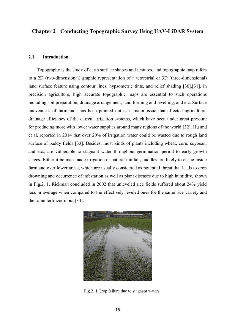
in Fig.2. 1. Rickman concluded in 2002 that unleveled rice fields suffered about 24% yield

loss in average when compared to the effectively leveled ones for the same rice variety and

the same fertilizer input [34].

Fig.2. 1 Crop failure due to stagnant waters

17

As precision land levelling facilitates surface drainage, improves crop establishment,

reduces occurrence of infestation and plant diseases, and increases crop yield [35], many

researchers both in academia and industry have proposed different methodologies on

removing mounds and puddles inside farmland. Apart from conventional land preparation

using ploughs and harrows after each crop season, generally two major proven techniques

that have already been put into practice for precision land levelling could be enumerated:

laser-assisted land levelling and GNSS based land levelling [36]. Nowadays not only in

developed countries like the United States and Japan but also in developing countries such as

China, India, and Brazil, laser-assisted land levelling techniques are gaining momentum

rapidly, as it works in a simple fashion [37]: the laser transmitter continuously emits a laser

plane, which is intercepted by the laser receiver in real time so that the height deviation to the

target height plane could be calculated; the height deviation is sent to the control box, and the

scraper automatically goes up and down according to commands from the control box aiming

at minimizing the deviation between the laser receiver and the target height plane; as the

scraper adapts the height, soil of higher ground is cut and hold in the bucket until it is carried

to lower ground and got released. Furthermore, Li and et al. in 2012 developed an attitude

measurement system for scraper of a laser-controlled land leveler by fusing data from a tri-

axial accelerometer and a digital gyroscope, which made the whole levelling system work

more efficiently and reliably [38]. Although it is explicit in structure and easy to operate,

laser-assisted land leveler has its inherent flaws: the selection of location and preset height of

the laser transmitter determines the cutting depth of each location (cut/fill ratios) directly, and

without an accurate topographic land survey it is next to impossible to optimized the volumes

of relocated earth. It is not unusual that operators find out that most of the time the scraper

hangs too high to cut any soil (idle operation), or worse, the tractor gets stuck and slips over

one spot and cannot move forward due to insufficient power when the cutting depth becomes

too large.

On the other hand, GNSS based land leveler came into practical application since mid-

1990s, when RTK-GPS service finally entered the market with an acceptable price and

centimeters-accuracy for measurements of 3D positions (latitude, longitude, and altitude).

GNSS based land leveler uses a GNSS receiver to measure 3D coordinates of the scraper and

adjusts the scraper’s height by comparing the current altitude with the desired one to

complete the earth-moving operation [39]. But, it shares the same drawback with the laser-

assisted land leveler: the GNSS based land leveler also needs an extra land survey, usually by

18

driving the GNSS receiver equipped tractor throughout the farmland prior to levelling

operation in order to acquire an farmland surface elevation map. According to the elevation

map drivers could preset an optimal ground height of each field and calculate cut/fill ratios

for each point by using GIS technology. Either way, whether it is a laser-assisted land leveler

or a GNSS based one, topographic survey is usually prerequisite, and land levelling accuracy,

efficiency, as well as energy consumption is in high accordance with the delicacy of each

topographic map of the farmland.

In order to generate topographic maps, new technologies including terrestrial laser

scanning, airborne laser scanning, and aerial photogrammetry are recently utilized for

different kinds of engineering applications like construction site, urban ecology modeling,

forest monitoring, and etc. [40]-[44]. Whist theodolite, total station, and RTK-GPS module

remain the conventional and primary methods that are used in common topographic

surveying. Theodolite is a precise instrument for measurement of angles in both horizontal

and vertical dimensions since sixteenth century; and total station is an all-electronic device

developed from theodolite on the theory of electronic distance measurement [45]. Resop and

et al. in 2010 compared different surveying techniques by using traditional total station and

terrestrial laser scanner to monitor streambank retreat, and concluded that surveying error of

total station would be significant when extrapolating to a certain reach, whist terrestrial laser

scanner provides much more detailed spatial information [46]. Corsini and et al. in 2013

monitored and mapped a slow moving compound rock slide by integration of airborne laser

scanner, terrestrial laser scanner, and automated total station, which quantified slope

movement in the order of centimeters to a few decimeters [47]. Pablo and et al. in 2017

evaluated a mobile LiDAR system mounted on a car to develop an architectural analysis by

generating 3D point cloud [48]. There are also plenty of research works and products

providing digital surface model and digital elevation model based on airborne

photogrammetry or satellite stereo-imagery [49]-[51], but the spatial resolution as well as

vertical accuracy of such topographic maps generated from photogrammetric processing

usually reaches several decimeters to tens of meters, which makes it unsuitable to be used in

farmland for precision land leveling operation.

Therefore, in this study, we introduced a low-altitude UAV equipped with a high

precision one-dimensional LiDAR (Light Detection and Ranging) distance measuring device

to conduct topographic survey in a simple and totally autonomous manner. The research

19

objective is to integrate data of multiple sensors including LiDAR, MEMS IMU, and PPK

(Post Processing Kinematic) GPS receivers, to generate a topographic map at farmland level

by using a low-altitude UAV-LiDAR system. The accuracy of the UAV-LiDAR system

based topographic surveying was validated by acquiring the corresponding RTK-GPS

coordinates and through visual inspection as well.

2.2 Research Platform and Equipment

In this research we developed a UAV-LiDAR topographic surveying system by installing

a one-dimensional LiDAR distance measuring device, a mini-computer, an external GPS

rover receiver for PPK-GPS positioning, and other peripheral devices such as battery banks

and an external GPS antenna on a small UAV. Each battery bank is meant for powering the

LiDAR, the mini-computer, and the external GPS module, respectively.

2.2.1 UAV Platform and Built-in Sensors

As described in Sector 1.1.4, a hexa-copter (ENROUTE CO., LTD., Fujimino, Japan)

was used as the small UAV platform in this study, shown in Fig.2. 2. This is a high-powered

industrial UAV, which is originally designed for agricultural chemical spraying with the

payload capacity of 6.6 kg. We altered the bottom part of this UAV so that the LiDAR, mini-

computer, as well as battery banks could be fixed upon the UAV platform. The UAV itself

uses two LiPo batteries and each of them is comprised of 6 battery chips (cells), which are

separated and protected by aluminum plates. These LiPo batteries are capable of powering

the no-load UAV for a 20-minute flight, however, as the payload increases the flight

endurance become shorter. In the case of our developed UAV-LiDAR topographic surveying

system, the maximum flight endurance reached up to about eight minutes when flying at the

ground speed of 5 m/s and 30 meters above ground level. The specifications of the UAV are

listed in Table 2. 1.

Table 2. 1 Specifications of the UAV platform

Overall size (with propellers uninstalled) Φ1397*450mm

Propeller size 457.2mm

Battery type LiPo 6 Cell

Battery capacity* number 99 Wh *2

Total number of Motor 6

Motor type Zion5828-340KV

20

Weight 5.4 kg

Payload capacity 6.6 kg

Maximum climbing speed 5 m/s

Maximum flight speed 20m/s

Wind resistance 10 m/s

Fig.2. 2 A small UAV used in this study

This UAV utilizes an industrial standard PIXHAWK autopilot hardware as an onboard

flight controller, which is designed by 3D Robotics Inc. in collaboration with ArduPilot

Group. The PIXHAWK flight controller integrates several kinds of inertial MEMS sensors

including a 3D accelerometer, a gyroscope, a magnetometer, and a barometer, which utilizes

a high accurate and reliable algorithm for acquiring attitude information of the UAV and

implementing self-balancing in real time. PIXHAWK flight controller could also records the

spatial position as well as the orientation or attitude information of the UAV platform in real

time when connecting with an external GPS module, which might be further analyzed for

correcting LiDAR’s distance measurements in this study. It has various kinds of ports that are

ready to be connected with multiple sensors for augmentation purpose, shown in Fig.2. 3.

Interface 1 is reserved for the digital spectrum modulation system, which is a newly released

radio technology offering an interference-immune and impenetrable radio link; Interface 2 is

for remote monitoring on GCS; Interface 3 is for remote monitoring controller; Interface 4 is

for universal serial bus communication; Interface 5 is a serial peripheral interface; Interface 6

is for power unit; Interface 7 is for safety switch function; Interface 8 is for buzzer function;

Interface 9 is for serial communicating; Interface 10 is for external GPS module; Interface 11

21

is for controller area network; Interface 12 is for inter-integrated circuit; Interface 13 is for

analog-digital-converter to 6.6 voltage; Interface 14 is for analog-digital-converter to 3.3

voltage; and interface 15 is for light-emitting diode display.

Fig.2. 3 PIXHAWK flight controller

2.2.2 LiDAR and Onboard Computer

LiDAR is originally a portmanteau term of Light Detection and Ranging, Light Imaging

Detection and Ranging, and Laser Imaging and Ranging, which is a surveying method of

measuring distance to a target by emitting a pulsed laser light and calculating the time or the

changes of phase of the returned laser light [52]. LiDAR has a wide range of applications

from meteorology to terrestrial mapping, vegetation coverage, and etc., based on the data’s

purpose and targeting objects. It could also be divided into terrestrial LiDAR applications and

airborne LiDAR applications, according to different kinds of platforms. Within the category

of airborne LiDAR applications it could further be divided into low-altitude airborne LiDAR

applications and high-altitude airborne LiDAR applications, and both of them create 3D point

cloud models. Low-altitude airborne LiDAR is currently the most efficient, detailed and

accurate method of generating a digital surface model (DSM), while the high-altitude

airborne LiDAR provides a bigger coverage with a reduction in distance measuring accuracy

and spatial point density, shown in Fig.2. 4.

22

Fig.2. 4 Airborne LiDAR application

However, as shown in Fig.2. 4, in order to obtain accurate distance measurements and

geographical coordinates for each measurement, the commercial airborne LiDAR system

incorporate expensive RTK-GPS module and IMU sensors onboard. For small UAVs, there is

not enough room for these extra but necessary auxiliary devices both physically and

economically. Thus, in this study we introduced a high precision one-dimensional LiDAR

device (Jenoptik, Jena, Germany) and took advantage of the inherent MEMS IMU sensors of

the UAV platform’s flight controller. The LiDAR distance measurement device is featured

with time-of-flight measurement principle and has a measuring range up to 300 m on natural

surfaces and 1 mm measuring resolution at the measuring frequency of 2000 Hz. Besides, the

LiDAR distance measurement is equipped with two lasers, shown in Fig.2. 5: part 1 is

transmitter optics and part 2 is pilot laser transmitter optics for collimation, whilst part 3 is

receiver optics. The safety level of the laser for distance measurement is class 1, which means

any case of injury of the unaided eyes of human can be excluded; whilst the safety level of

the pilot laser is class 2, which means that human eye can be protected by the eyelid closure

reflex against a short accidental look into the pilot laser beam without any additional

protection appliances. Another advantage of this LiDAR distance measurement device is that

the supply voltage has a wide range from 10 V to 30 V (direct current), which is basically

immune to voltage instability and provides reliable continuous measurements. The power

consumption of 5 W is also very low, which is suitable for the small UAV use as it cannot

carry large volume battery bank onboard.

23

Fig.2. 5 Laser beam divergence and spatial resolution

Laser beam divergence, measured in milliradians (mrad) or degrees, is another important

parameter of LiDAR distance measuring device, which is an angular measure of the increase

in beam size with the distance from the transmitter optics where the laser beam emerges to a

target. For many distance measurement applications, the lower the divergence of the laser

beam is, the more preferable and accurate of the measurement becomes. In this study the

laser beam divergence of the LiDAR distance measurement device is 1.7 mrad, and the

spatial resolution of each measurement is about 60 mm * 20 mm when measuring from a

distance of about 30 m, shown in Fig.2. 5.

The LiDAR distance measuring device provides various kinds of interfaces to be

connected with a computer including RS232, RS422, and Profibus. A mini-computer is used

to control as well as monitor the distance measuring operation, and at the same time to log

and save each distance measurement onboard in real time. We adopted a light and compact

mini-computer (GB-XMI1-3537, Gigabyte, Taiwan, China) in this study shown in Fig.2. 6,

and utilized a USB 3.0 (Universal Serial Bus) port to connect with the LiDAR distance

measuring device using a USB serial cable type A to D-sub 9 converter. The power supply of

the mini-computer is 19 V DC, and the power consumption is about 65 W. The specifications

of the LiDAR device and the mini-computer are listed in Table 2. 2.

1

2

3

24

Fig.2. 6 On board mini-computer

Table 2. 2 Specifications of LiDAR and onboard computer

LiDAR device

Dimensions 136 mm * 57 mm * 104mm

Weight 800 g

Measuring resolution 1 mm

Beam divergence 1.7 mrad

Measuring laser wavelength 905 nm

Pilot laser wavelength 635 nm

Supply voltage 10 V to 30 V DC

Power consumption < 5 W

Operating temperature -40°C to +60°C

Operating humidity 15% to 90%

Onboard computer

Dimensions 30 * 108 * 115 mm

Weight 400 g

Operating system Windows 32/64 bit

CPU Intel® Core™ i7-3537U 2GHz / 3.1GHz

Memory 8 Gigabyte

Interfaces 1 HDMI, 1 mini display port, 2 USB 3.0

Power supply DC 19 V

Power consumption 65 W

2.2.3 PPK-GPS modules and RTK-GPS modules

25

Table 2. 3 Specifications of PPK-GPS modules

GNSS receivers U-blox NEO-M8T

Processing unit Intel Edison

Dimensions 45.5 * 27 * 9.2 mm

Weight 14 g

Antenna Tallysman TW4721

Antenna dimensions 38 * 38 *14.3 mm

Antenna weight 50 g

Supply voltage 4.75 V to 5.5 V DC

Average power consumption 1 W

Operating temperature -20°C to +65°C

Antenna DC bias 3.3 V

Internal storage 2 Gigabyte

Signals GPS/QZSS L1, GLONASS G1, BeiDou B1

Galileo E1, SBAS Channels 72

As mentioned in Sector 1.1.2, the positioning accuracy of standalone GPS mode, DGPS

mode, and RTK-GPS mode is reported to be around 5 m, 1 m, and 2 cm, respectively. The

RTK-GPS modules are usually used as a supplemental set outfit together with an IMU device

when airborne LiDAR operations are under conduction. However, the commercial RTK-GPS

module is too large in size and too heavy to be installed upon our small UAV platform.

Besides, the cost of RTK-GPS service as well as the hardware is still a whopping price for

individual users. Therefore, we introduced a small and lightweight PPK-GPS module in this

study, which compromises of two identical GNSS receivers with the antenna and power

supply module. One GNSS receiver remains stationary as a ground base station, whilst the

other GNSS receiver is installed on the UAV-LiDAR topographic surveying system, shown

in Fig.2.7, and works as a rover receiver within twenty kilometers away from the ground base

station. The coordinates of the ground base station could be acquired by two ways. The most

precise method is to measure the location’s 3D coordinates (longitude, latitude, and altitude)

using a RTK-GPS module prior to or after the experiment, which provides an absolute and

accurate reference for PPK algorithm. The other one is a cost-efficient and easy to implement

approach, which only utilizes the raw GNSS data of ground base station and average the

location measurements for over thirty minutes up to two hours using least square method for

example. The averaged 3D coordinates of the ground base station usually reaches up to a 0.5

26

m accuracy, but it only deviates the rover GNSS module’s absolute location and the relative

centimeter level accuracy is unaffected. This high precision GNSS positioning outfit utilizes

an open source program package RTKLIB, which supports standard and precise positioning

algorithm with GPS, GLONASS, Beidou, Galileo, and QZSS, using post processing analysis

methods.

Table 2. 4. Specifications of RTK-GPS module

Receiver Topcon GB-3

Dimensions 240 * 110 * 35 mm

Weight 600 g

Supply voltage 6 V to 28 V DC

Average power consumption 3.5 W

Operating temperature -40°C to +75°C

Internal storage 2 Gigabyte

Signals GPS, GLONASS

Channels 72

RTK accuracy Horizontal: 10 mm

Vertical: 15 mm Antenna PG-S1

Antenna dimensions 141.6 * 141.6 *54.2 mm

Antenna weight 615 g

RTK-GPS module was also used to validate the accuracy of the topographic map

generated from the UAV-LiDAR topographic surveying system. RTK-GPS receiver working

in a virtual reference station fashion usually provides a reliable and high precision 3D

coordinates (longitude, latitude, and altitude) up to 2 cm, which has a wide range of

applications in surveying as well as in the domain of autonomous driving. In this study we

used a Topcon RTK-GPS receiver with a PG-S1 antenna (TOPCON Cor., Tokyo, Japan) to

record reference 3D coordinates, shown in Fig.2.7, where part 1 marked in green box is the

PPK-GPS receiver installed on the UAV platform and part 2 marked in red box is the RTK-

GPS receiver for comparison. The specifications of the RTK-GPS receiver as well as antenna

are listed in Table 2. 4.

27

Fig.2.7 RTK-GPS module and PPK-GPS module

2.3 Methodology

Fig.2. 8 Approach of generating topographic map

The overall approach of farmland topographic surveying by using the UAV-LiDAR

system consists of six major steps: acquisition of raw data from LiDAR, MEMS IMU, and

GNSS base as well as GNSS rover receivers; acquisition of PPK-GPS coordinates; correcting

LiDAR distance measurements with attitude information from MEMS IMU; synchronizing

PPK-GPS data with corrected LiDAR distance measurements; generating topographic map

and validating the topographic map generated from UAV-LiDAR system using combine

○1

□2

28

harvester’s RTK-GPS data, shown in Fig.2. 8. This study adopted World Geodetic System

1984, or WGS84, and map projection of UTM (Universal Transverse Mercator) Zone_54N

with datum of WGS84, as the coordinate system in this paper, if not particularly indicated.

2.3.1 Field Site and Experiment Description

Fig.2. 9 A harvested wheat field under study

UAV-LiDAR system based topographic surveying experiment was established over a

harvested wheat field located in Sapporo, Hokkaido, Japan, which accounts for about 0.4

hectare, shown in Fig.2. 9. High accuracy LiDAR device was fixed under the UAV platform

pointing vertically downwards (shown in Fig.2. 2), and raw distance measurements data from

the LiDAR device are ready to be corrected by using attitude data calculated from a tri-axial

MEMS accelerometer, a tri-axial MEMS gyroscope, and a tri-axial MEMS magnetometer.

Ground base station of the PPK-GPS module was measured and recorded by using the RTK-

GPS module that were described in Sec. 2.2.3, whilst the rover receiver was attached on the

top of the UAV platform. Autonomous flight was conducted on 10 August 2017, using flight

paths that were designed beforehand at the speed of about 5 m/s and about 30 meters above

ground level. Trajectory (two round trips) of the flight in blue color with the cross track

interval of about 6 meters is shown in Fig.2. 9. As the output frequency of LiDAR distance

29

measurements and PPK-GPS data was synchronized at 10Hz, along track interval of each

surveying point can be calculated as about 0.5 meter.

Besides, RTK-GPS data was also acquired by installing the Topcon GB-3 RTK-GPS

receiver and the PG-S1 antenna on a combine harvester on 21 July 2017 when wheat

harvesting was conducted in autonomous driving mode. The Topcon RTK-GPS module

worked in a virtual reference station fashion, receiving correction information from GPS base

station through network. The trajectory of the combine harvester based RTK-GPS was also

shown in Fig.2. 9 in black color with the cross track interval of about 1.6 meters and along

track interval of each surveying point of about 0.2 m.

2.3.2 Acquisition of UAV-LiDAR System’s Attitude Information

The small UAV platform used in this study consists of six brushless DC motors, with

three pairs of counter-rotating propellers which are fixed-pitch blades. These three pairs of

counter-rotating propellers not only act as a propulsion system but also control and stabilize

the UAV platform’s attitude by changing the angular speed of each pair of motors, so that

such movements like climbing, descending, turning direction, whirling, and even obstacle

avoiding could be implemented. The rotational speed of each brushless motor is determined

by the voltage imposed upon the motors, as Eq. (2.1).

eC

IRUn (2.1)

where:

n is the rotational speed of each motor;

U is the voltage imposed upon each motor;

I is the DC current through each motor;

R is the equivalent resistance of each motor’s coil;

motor theof ariableconstant v theis eC ;

and is the magnetic flux of each motor’s coil.

30

In order to describe movements of the UAV platform, usually two reference systems are

necessary. One is the earth fixed reference system using north, east, and down coordinates,

which is tangent to the earth surface. The other one is a body fixed reference system, centered

in the UAV platform’s center of gravity. The absolute position (x, y, z) of the UAV is defined

as linear to the body fixed reference system’s origin, whilst the angular position of the UAV

is usually described by means of the Euler angles defined as pitch (θ), roll (ϕ), and yaw (ψ).

And thus, the transformation from the body reference system [ 𝜃 𝜙 𝜓]T to the earth reference

system [x y z]T can be realized by using the rotation matrix R [53].

𝑅 = [

𝑐𝑜𝑠𝜃𝑐𝑜𝑠𝜓 𝑐𝑜𝑠𝜓𝑠𝑖𝑛𝜃𝑠𝑖𝑛𝜙 − 𝑐𝑜𝑠𝜙𝑠𝑖𝑛𝜓 𝑐𝑜𝑠𝜙𝑐𝑜𝑠𝜓𝑠𝑖𝑛𝜃 + 𝑠𝑖𝑛𝜙𝑠𝑖𝑛𝜓𝑐𝑜𝑠𝜃𝑠𝑖𝑛𝜓 𝑐𝑜𝑠𝜙𝑐𝑜𝑠𝜓 + 𝑠𝑖𝑛𝜃𝑠𝑖𝑛𝜙𝑠𝑖𝑛𝜓 𝑐𝑜𝑠𝜙𝑠𝑖𝑛𝜃𝑠𝑖𝑛𝜓 − 𝑐𝑜𝑠𝜓𝑠𝑖𝑛𝜙

−𝑠𝑖𝑛𝜃 𝑐𝑜𝑠𝜃𝑠𝑖𝑛𝜙 𝑐𝑜𝑠𝜃𝑐𝑜𝑠𝜙] (2.2)

Therefore, acquisition of attitude information (θ, ϕ, ψ) of the UAV body is essential to

control and stabilize the UAV, and also necessary for further analysis using attitude

information to correct LiDAR distance measurements. 3D MEMS gyroscope is an inertial

sensor for measuring orientation based on angular momentum principles, and the tri-axial

angles [𝜃𝑔𝑦𝑟𝑜 𝜙𝑔𝑦𝑟𝑜 𝜓𝑔𝑦𝑟𝑜]T can be acquired by integral operation of angular speed of each

axle, shown in Eq. (2.3). However, due to temperature variations of the MEMS gyroscope

during operation, drift error of gyroscope and will accumulate along with time and accuracy

as well as reliability of the attitude information calculated from a sole MEMS gyroscope

would be compromised. On the other hand, 3D MEMS accelerometer can also be used to

measure UAV’s orientation based on the trigonometric functions of the acceleration of

gravity components in each axial, shown in Eq. (2.4) and Eq. (2.5). But, the accelerometer is

incapable of distinguishing the acceleration of gravity from external vibration, which means

it is not suitable for attitude estimation application in cases of severe agitation such as aerial

vehicles.

[ 𝜃𝑔𝑦𝑟𝑜 𝜙𝑔𝑦𝑟𝑜 𝜓𝑔𝑦𝑟𝑜]𝑇

= ∫[𝜔𝑥 𝜔𝑦 𝜔𝑧]𝑇

𝑑𝑡 (2.3)

where 𝜃𝑔𝑦𝑟𝑜 , 𝜙𝑔𝑦𝑟𝑜,and 𝜓𝑔𝑦𝑟𝑜 is the calculated pitch, roll, and yaw of UAV platform from

gyroscope, respectively; whilst ωx , ωy, and ωz is the raw rotation rates (degree/s) of each

axial from the gyroscope, shown in

Fig.2. 10, at the sampling frequency of 50 Hz.

31

𝜃𝑎𝑐𝑐𝑒 = −arcsin (𝑔𝑥

√𝑔𝑥2+𝑔𝑦

2+𝑔𝑧2) (2.4)

𝜙𝑎𝑐𝑐𝑒 = 𝑎𝑟𝑐𝑡𝑎𝑛 (𝑔𝑦

𝑔𝑧) (2.5)

where 𝜃𝑎𝑐𝑐𝑒 and 𝜙𝑎𝑐𝑐𝑒 is the calculated pitch and roll of the UAV from accelerometer,

respectively; whilst gx, gy, and gz is the readings of acceleration components in each axial

from the accelerometer, shown in Fig.2. 11, at the sampling frequency of 50 Hz.

32

Fig.2. 10 Rotation rates of gyroscope

33

Fig.2. 11 Raw accelerometer values

34

Fig.2. 12 Pitch, roll and yaw values of the UAV-LiDAR system

Moreover, magnetometer was also used as a complementary sensor for calculating the

change of heading (yaw) of the UAV, in combination with the above mentioned gyroscope

and accelerometer, as neither of them can be used solely for satisfactory attitude estimation in

long time operations. There are more than one well-proved method for data fusion of

gyroscope, accelerometer, and magnetometer in the domain of UAV attitude control, such as

the explicit complementary filtering method, self-adaptive complementary filtering method,

35

gradient descent filtering method, Kalman filtering method as well as extended Kalman

filtering method, and etc. In this study the UAV’s flight controller utilizes an extended

Kalman filter to fuse data from multiple sensors of accelerometer, gyroscope, and

magnetometer for attitude estimation. The attitude estimation system is simplified as Fig.2.

13, whilst mx, my, mz, and ψmagn

is the magnetic intensity components in each axial and

estimated yaw from magnetometer, respectively. In this way, attitude data of pitch, roll, and

yaw values of the UAV-LiDAR system were acquired after the flight at the sampling

frequency of 10 Hz, shown in Fig.2. 12. Attitude data of pitch and roll were used to correct

LiDAR distance measurements for further analysis.

Fig.2. 13 Simplified attitude estimation system of the UAV

2.3.3 Synchronizing LiDAR Distance Measurements with PPK-GPS Data

Table 2. 5 PPK-GPS coordinates (in part)

Sample

Number

Date UTC Latitude(degree) Longitude(degree) Altitude(m)

1 8/10/2017 01:04.2 43.0735617 141.3354461 14.078

2 8/10/2017 01:04.3 43.0735617 141.335446 14.078

3 8/10/2017 01:04.4 43.0735617 141.3354461 14.077

4 8/10/2017 01:04.5 43.0735617 141.3354461 14.077

5 8/10/2017 01:04.6 43.0735617 141.335446 14.079

… … … … … …

4740 8/10/2017 08:58.1 43.0735336 141.3354268 14.263

4741 8/10/2017 08:58.2 43.0735336 141.3354268 14.265

4742 8/10/2017 08:58.3 43.0735336 141.3354268 14.261

Accelerometer

Gyroscope

Magnetometer

𝑤𝑥 , 𝑤𝑦,𝑤z

𝑚𝑥 , 𝑚𝑦,𝑚𝑧

𝜃𝑎𝑐𝑐𝑒, 𝜙𝑎𝑐𝑐𝑒

𝜃𝑔𝑦𝑟𝑜 , 𝜙𝑔𝑦𝑟𝑜, 𝜓𝑔𝑦𝑟𝑜

𝜓𝑚𝑎𝑔𝑛

Extended

Kalman

Filter

Pitch (𝜃),

Roll (𝜙),

Yaw(𝜓)

36

PPK-GPS data were acquired by using an open source algorithm in RTKLIB software,

after measuring absolute geo-spatial coordinates of ground base station as correction

reference using a RTK-GPS module. The 3D coordinates was measured as (43.07355556 N,

141.3354386 E, 11.236 m). Considering the RTK-GPS module in the topographic map’s

validation experiment is installed on the top of the combine harvester’s cabin, which is about

2.71 m above ground level, the altitude of the base station was rectified as 13.946 m by

adding the RTK-GPS module’s height of 2.71 m to the measured altitude 11.236 m. Thus, the

PPK-GPS coordinates of the GNSS rover, which is attached to the UAV-LiDAR system,

were calculated and listed in Table 2. 5. The number of samples of PPK-GPS measuring

reached up to 4742 in total at the frequency of 10 Hz.

Fig.2. 14 Raw data of PPK-GPS altitudes and LiDAR distance measurements

Fig.2. 15 Synchronized PPK-GPS altitudes and LiDAR distance measurements

37

As mentioned in Sec. 2.2.2, the LiDAR device used in this study measures distance at the

frequency of 2000 Hz with the measuring resolution of 1 mm. Because the output frequency

of PPK-GPS coordinates as well as the attitude data of the UAV-LiDAR system is fixed as 10

Hz, the LiDAR distance measurements cannot be directly corrected by using the attitude

information, nor can it be directly aligned with the PPK-GPS coordinates. Besides, as the

LiDAR distance measurement’s output has no timestamp, it has to be synchronized with

PPK-GPS data in the first place so that each LiDAR distance measurement could be tagged

with timestamp, and then be aligned with the attitude data using timestamp and be further

corrected by using the attitude data. In order to synchronize the 2000 Hz LiDAR distance

measurements with the 10 Hz PPK-GPS coordinates as well as to improve measuring

precision, a mean filter was applied to the LiDAR distance measurements so that the output

was averaged from 2000 Hz to 10 Hz. The PPK-GPS altitude values and the averaged LiDAR

distance measurements are shown in Fig.2. 14. Subsequently, taking LiDAR distance

measurements and PPK-GPS altitude that are on the point of taking off as a benchmark, we

synchronized two sets of height data so that each LiDAR distance measurement could be geo-

coded and timestamped. The synchronized result of corrected LiDAR distance measurements

with PPK-GPS altitude was shown in Fig.2. 15.

2.3.4 Correcting LiDAR Distance Measurements and Calculating Ground Elevation

As shown in Fig.2. 12, the attitude of the UAV-LiDAR system is apt to be changing all

the time during each flight, due to inherent aerodynamic characteristics. The changing

attitude of the UAV-LiDAR system impairs the accuracy of each LiDAR distance

measurement, as the LiDAR device is rigidly fixed upon the UAV platform pointing

downwards. Because each LiDAR distance measurement has already been geo-coded and

timestamped by synchronizing with PPK-GPS data, we sued the timestamp information on

the LiDAR distance measurements and attitude data of the UAV-LiDAR system to

synchronize them together. Therefore, in order to eliminate such effects of continuously

changing attitudes of the UAV-LiDAR system during the flight on the LiDAR distance

measurements, synchronized attitude data of pitch and roll were utilized to correct the LiDAR

distance measurements using the model expressed as Eq. (2.6). The corrected LiDAR

distance measurements were shown in Fig.2. 16.

coscos ddcorr (2.6)

38

where corrd , d , 𝜃 , and 𝜙 indicates the corrected LiDAR distance measurements above

ground level, the raw LiDAR distance measurement, and the attitude data of pitch and roll,

respectively.

Fig.2. 16 Corrected LiDAR distance measurements

Based on the synchronized results of corrected LiDAR distance measurements with

PPK-GPS 3D coordinates, ground elevation of each surveying point could be calculated

using the model expressed as Eq. (2.7). We removed superfluous data during the process of

taking off, turning round, and landing by visual inspection. And the total number of

surveying points within the field under study amounted to 1135 in total, shown in Fig.2. 17.

corrfixppkgps dhhe (2.7)

where e, hppkgps, hfix, and dcorr indicates the ground elevation of each surveying point, the PPK-

GPS altitude, the height difference between PPK-GPS rover receiver’s antenna and LiDAR’s

laser lens (0.36 m), and the corrected LiDAR distance measurement, respectively.

Fig.2. 17 Ground elevation of each surveying point

39

2.4 Result and Discussion

2.4.1 Accuracies of PPK-GPS Altitude and LiDAR Distance Measurements

Fig.2. 18 Accuracy of PPK-GPS coordiantes

Fig.2. 19 Accuracy of LiDAR distance measurements

To validate the accuracies of PPK-GPS coordinates, we extracted 6000 sets of PPK-GPS

data consecutively ten minutes before the UAV-LiDAR system took off when the PPK-GPS

rover’s antenna was hold stationary. The horizontal and vertical accuracy of PPK-GPS

coordinates was shown in Fig.2. 18, from which we may conclude that the horizontal

accuracy is as good as about 0.01 m (1cm), as most of the 6000 set of easting and northing

coordinates fall within the range of about 0.01m. On the other hand, from Figure 8 we may

understand that altitude measurements of PPK-GPS changed along with time, mainly due to

adoption of different combinations of satellites over time. The altitude measurements varied

from about 115.735 m to 115.755 m with vertical accuracy of about 0.02 m (2 cm). Besides,

another 6000 sets of static LiDAR distance measurements were also acquired by pointing the

LiDAR device at a wall about 25 m far away and holding it still for ten minutes, shown in

Fig.2. 19. From Figure 9 we could conclude that LiDAR distance measurements remained

40

substantially constant over time, mostly ranging from 25.872 m - 25.882 m, and the

measuring accuracy could be confirmed as within 0.01 m (1 cm). Thus, we may declare that

the accuracy of this high accurate topographic surveying outfit surpasses the dominant

handheld RTK-GPS based topographic surveying device.

2.4.2 Validating UAV-LiDAR Based Topographic Surveying Accuracy

Based on the calculated ground elevation of each surveying point, a map indicating

spatial variations of within-field ground elevation was generated by using GIS (Geographic

Information System) software ArcMap (ESRI Inc., Redlands, AB, Canada), shown in Fig.2.

20. From the graduated symbols representing different levels of ground elevation, we can

visually understand the general high-north-low-south terrain of the field under study, with the

ground elevations varying from 13.237 m to 14.594 m. From Fig.2. 20 we may also conclude

that the area that is marked in green box has relatively low ground elevation, and the influx of

irrigation water as well as snowmelt water or heavy rainfall is very likely to form puddles,

which pose potential threaten to the crop growth and yield. In order to achieve uniform

growth status of crops and improved yield, an east-west direction’s land leveling operation

could be suggested to effectively fill the puddles and remove the mounds.

Fig.2. 20 Ground elevation of each surveying point showed in graduated symbols

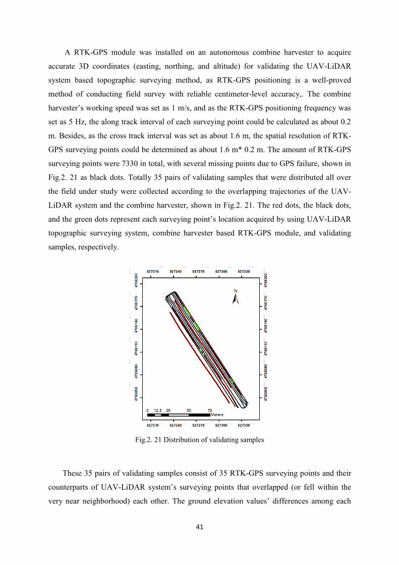
41

A RTK-GPS module was installed on an autonomous combine harvester to acquire

accurate 3D coordinates (easting, northing, and altitude) for validating the UAV-LiDAR

system based topographic surveying method, as RTK-GPS positioning is a well-proved

method of conducting field survey with reliable centimeter-level accuracy,. The combine

harvester’s working speed was set as 1 m/s, and as the RTK-GPS positioning frequency was

set as 5 Hz, the along track interval of each surveying point could be calculated as about 0.2

m. Besides, as the cross track interval was set as about 1.6 m, the spatial resolution of RTK-

GPS surveying points could be determined as about 1.6 m* 0.2 m. The amount of RTK-GPS

surveying points were 7330 in total, with several missing points due to GPS failure, shown in

Fig.2. 21 as black dots. Totally 35 pairs of validating samples that were distributed all over

the field under study were collected according to the overlapping trajectories of the UAV-

LiDAR system and the combine harvester, shown in Fig.2. 21. The red dots, the black dots,

and the green dots represent each surveying point’s location acquired by using UAV-LiDAR

topographic surveying system, combine harvester based RTK-GPS module, and validating

samples, respectively.

Fig.2. 21 Distribution of validating samples

These 35 pairs of validating samples consist of 35 RTK-GPS surveying points and their

counterparts of UAV-LiDAR system’s surveying points that overlapped (or fell within the

very near neighborhood) each other. The ground elevation values’ differences among each

42

pair of validating samples were shown in Fig.2. 22, from which we can conclude that the

ground elevation values of UAV-LiDAR system based topographic surveying points correlate

well with the ones of RTK-GPS’s altitude values. We can also see that the ground elevation

values of RTK-GPS are smoother than the ones of the UAV-LIDAR system, as the combine

harvester that carries the RTK-GPS module follows the field terrain closely and all residual

straws or standing plants would be crushed below the chassis due to heavy dead weight of the

vehicle. On the other hand, as explained in Sec. 2.2.2 the UAV-LiDAR system measures the

field terrain in an area-scanning fashion (about 6 cm * 2 cm when flying at the height of 30 m

above ground level) rather than a point-measuring fashion like the RTK-GPS module

installed on the combine harvester due to laser beam divergence. Within the scanning area

there might be the existence of residual straws or standing plants over the harvested wheat

field, which poses as a potential outlier in the ground elevation survey.

Fig.2. 22 Differences among validating samples’ ground elevation

Finally, according to Eq. (2. 8) the Root Mean Square Error (RMSE) between these 35

pairs of ground elevation data of RTK-GPS and UAV-LiDAR system was calculated as 0.035

m (3.5 cm). Considering that the ground elevation of the field under study varies from 13.237

m to 14.594 m according to the topographic survey using the UAV-LiDAR system, the value

of the RMSE is acceptable in comparison with the elevation difference of 1.357 m, which

indicates that the UAV-LiDAR topographic surveying system is very precise.

𝑅𝑀𝑆𝐸𝑈𝐴𝑉−𝑅𝑇𝐾 = √∑ (𝑒𝑈𝐴𝑉𝑖−𝑒𝑅𝑇𝐾𝑖)35𝑖=1

2

35 (2.8)

43

where 𝑒𝑈𝐴𝑉𝑖 and 𝑒𝑅𝑇𝐾𝑖 indicates the ground elevation data of the UAV-LiDAR system and

the RTK-GPS data, respectively.

2.4.3 Visual Validation of UAV-LiDAR System Based Topographic Survey

An experiment was also established over a harvested sugarcane farmland located in

Mackay, Queensland, Australia (around 21.259794°S–21.263142°S and 149.091325°E–

149.094109°E), shown in Fig.2. 23, which accounts for about 3 hectares. Autonomous flight

using the same UAV-LiDAR topographic surveying outfit was conducted in December 7

2016 at the ground speed of 5 m/s and altitude about 30 meters above ground level.

Trajectory of the flight also was shown in Fig.2. 23 as red dots, and the track intervals were

set every 20 m. In order to confirm the UAV-LiDAR system’s working capability, several

bumps and hollows (about 30 cm in depth and 1.5 m in length) were artificially built inside

the field by using a plough attached to a tractor, shown in Fig.2. 24. From Fig.2. 25 we can

clearly see that two hollows under the flight trajectory of the UAV-LiDAR system were

precisely spotted, showed in black circle and rectangle, respectively. And we can come to the

conclusion that the UAV-LiDAR topographic surveying system has good capability of

conducting a farmland topographic survey for precision land leveling.

Fig.2. 23 Field site of experiment for visual validation

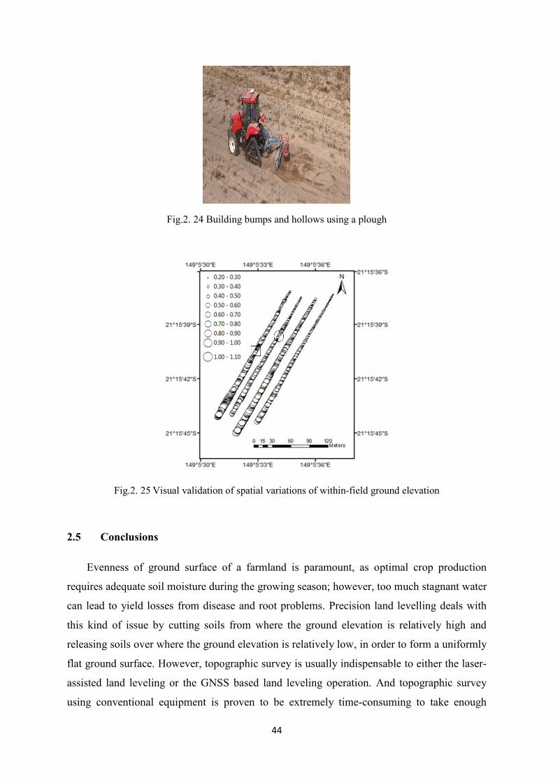
44

Fig.2. 24 Building bumps and hollows using a plough

Fig.2. 25 Visual validation of spatial variations of within-field ground elevation

2.5 Conclusions

Evenness of ground surface of a farmland is paramount, as optimal crop production

requires adequate soil moisture during the growing season; however, too much stagnant water

can lead to yield losses from disease and root problems. Precision land levelling deals with

this kind of issue by cutting soils from where the ground elevation is relatively high and

releasing soils over where the ground elevation is relatively low, in order to form a uniformly

flat ground surface. However, topographic survey is usually indispensable to either the laser-

assisted land leveling or the GNSS based land leveling operation. And topographic survey

using conventional equipment is proven to be extremely time-consuming to take enough

45

samples manually, not even to say that the conduction itself is highly dependent on

professionals. In this study, we developed an innovative topographic surveying method by

integrating LiDAR distance measurements with PPK-GPS coordinates, using a low-altitude

UAV as a platform.

The accuracy of PPK-GPS altitude as well as the LiDAR distance measurements was

validated as 2 cm and 1 cm, respectively, which showed good capability of conducting

topographic surveying operations. We conducted a topographic surveying experiment in a

harvested wheat field using the UAV-LiDAR system, and the total number of surveying

points within the wheat field under study amounted to 1135 in total, when superfluous data

were removed during the process of taking off, turning round, and landing by visual

inspection. Ground elevation values of these topographic surveying points were calculated by

using the synchronized results of corrected LiDAR distance measurements with PPK-GPS

3D coordinates. Based on the calculated ground elevation of each surveying point, a map

indicating spatial variations of within-field ground elevation was generated by using GIS

software ArcMap. From the graduated symbols representing different levels of ground

elevation, we can understand the general high-north-low-south terrain of the field under study.

We may also visualize several puddles inside the wheat field, and accordingly an east-west

direction’s land leveling operation was suggested to effectively fill the puddles and remove

the mounds of the field.

Furthermore, in order to validate the accuracy of the ground elevation data of the UAV-

LiDAR topographic surveying system, a RTK-GPS module was utilized to acquire

topographic surveying data on the same field, as RTK-GPS positioning is a well-proved

method with reliable centimeter-level accuracy. Totally 35 pairs of validating samples that

were randomly distributed all over the field under study were collected according to the

overlapping trajectories of the UAV-LiDAR system and the RTK-GPS module. The RMSE

between ground elevation data of RTK-GPS and UAV-LiDAR system was calculated as

0.035 m. In consideration that the ground elevation of the field under study varies in the

range of 1.357 m according to the topographic survey data of the UAV-LiDAR system, the

RMSE of 0.035 m is considered as highly accurate and acceptable. Besides, an experiment in

a harvested sugarcane field was also conducted for visual validation of the working capacity

of the developed UAV-LiDAR topographic surveying system. Bumps and hollows in the

middle of the field artificially made by using a plough could be clearly spotted by visual

46

interpretation, which practically proved the applicability of this UAV-LiDAR system for

topographic mapping operations.

In short, the proposed UAV-LiDAR system based approach of conducting topographic

survey could practically provide ground elevation reference for laser-assisted land leveler to

preset the height of the laser transmitter, and also could be used to produce cut/fill ratio map

for GNSS based land leveler. And the topographic surveying system is of high precision,

efficient in time and cost, and simple in structure, which is also highly flexible in designing

and executing autonomous flight for each specific farmland.

47

Chapter 3 Integrating Aerial Photogrammetric DSM with UAV-LiDAR

System’s Topographic Surveying Data

3.1 Introduction

Precision land levelling deals with the issues of unevenness of the farmland ground

surface, and neither the laser-assisted land leveler nor the RTK-GPS guided land leveler can

deliver the optimal performance unless an accurate topographic map of the field is available

prior to land leveling operation. Generally, a topographic map is generated by interpolating

individual surveying points that are uniformly distributed around the area of interest. Total

station and portable RTK-GPS module are often used in common topographic surveying as

the conventional and primary tools, whilst terrestrial laser scanner, airborne laser scanner,

and aerial photogrammetry devices are recently utilized for different kinds of topographic

applications like construction site, urban ecology modeling, forest monitoring, and etc.

However, the time-consuming conventional topographic surveying methods as well as the

low vertical accuracy of the new fashioned topographic surveying techniques are not suitable

to generate precise topographic maps for farmland’s precision land leveling operation.

Besides, the overall accuracy of topographic maps not only depends on the accuracy of

each surveying measurements, but is also influenced by the spatial resolution as well as the

spatial distribution of the surveying points to a great extent. As it is well known that the

interpolating results are apt to be less reliable as the surveying points’ spatial resolution

increases. Basically, there are no other alternatives to improve the overall accuracy of an

interpolated topographic map but to increase the total number as well as the sampling spatial

resolution of the measured points, which is usually time-consuming or impossible to perform

in practice. On the other hand, aerial photogrammetric DSM is featured with great spatial

resolution, however, needs a large number of GCPs uniformly spreading around the area of

interest for guaranteeing the accuracy of the resulting surface elevation values.

Aerial photogrammetric DSM possesses the advantages of good spatial resolution and

large coverage, which has been utilized for many years in urban ecological study, forest

monitoring, and etc. But the processing of aerial images for generating photogrammetric

DSM usually needs strict camera calibration and well distributed ground control points

(GCPs). GCP in photogrammetry or computer vision domain refers to such features that are

48

easily recognizable and distinguishable in both the reality world and in the images during

post-processing, such like crossroads, bridges, field corners, and etc. The geospatial accuracy

as well as the ground elevation accuracy of the photogrammetric DSM is in high accordance

with the GCPs’ condition.

Furthermore, in recent years many commercial photogrammetric processing software

products emerged that are capable of generating point clouds, 3D models, and DSMs from

digital images based on computer vision techniques, which could find a wide range of

applications in 3D reconstruction and visualization, urban ecological surveying and mapping,

agricultural remote sensing and mapping, and etc. Agisoft PhotoScan (Agisoft LLC, St.

Petersburg, Russia) is one of the most advanced photogrammetric processing software

suitable for low-altitude UAV remote sensing. The Agisoft PhotoScan software utilizes the

latest multi-view 3D reconstruction theory for extracting key-points from each individual

aerial image, matching the identical key-points from multiple images, automatically

estimating camera parameters according to the image matching result, and finally stitching

multiple images into an ortho-mosaicked one.

Therefore, we came up with a solution of integrating the UAV-LiDAR system based

topographic surveying data, as described in Chapter 2, with the low-altitude UAV based

photogrammetric DSM for generating a precise topographic map. Because the topographic

surveying data using the UAV-LiDAR system is highly accurate but lacks adequate spatial

resolution when interpolated for generating topographic maps, whist the aerial

photogrammetric DSM is featured with great spatial resolution and rich details but cannot

guarantee the absolute accuracy of the pixels values (surface elevation values) that are away

from GCPs. In this chapter, we are to discuss the methodology of integrating these two

different sources of topographic data for generating a topographic map in an efficient and

accurate manner. This new topographic surveying method does not require the arrangement

of plentiful artificial GCPs for constraining the accuracy of each pixel’s ground elevation

value of the resulting aerial photogrammetric DSM, and does not need extra UAV-LiDAR

flights for acquiring a great deal of samples by shortening the cross-track intervals.

3.2 Methodology

In geo-statistics, interpolation is a method of approximating and assigning new data for

locations where no samples have been taken within the range of a discrete set of known data

49

points, as it is in practice always impossible to take samples at every location in an area of

interest due to restrictions of equipment or limited sampling time. Besides, interpolation is

commonly used to create continuous surface from data of discrete points in GIS domain for

better understanding of the overall trend and spatial variations, because real world

phenomenon are always continuous in nature such as ground elevation, depths of river,

temperatures, precipitations, and so on.

Interpolation results can vary significantly depending on different interpolating models,

since intermediate values for locations where no measurements are available are inferred by a

process based on different mathematical calculations. Piecewise constant interpolation is the

simplest interpolation model, which assigns the nearest known data value for the non-given

points. Nearest-neighbor algorithm is one of the most commonly used piecewise constant

interpolation method, which does not consider the values of neighboring points and only

selects the value of the nearest point for each interpolating location. This algorithm is very

easy to implement, and is usually used in digital imaging applications to select color values

for a textured surface. Besides, there are other interpolating models such as linear

interpolation, polynomial interpolation, spline interpolation, and Gaussian process regression

which is also known as Kriging, and etc. Each of the interpolating model suits specific needs

when used for building continuous maps. For example, Kriging interpolation originates from

geological mineral concentration analysis, whilst inverse distance weighting (IDW)

interpolation is best suitable for demographical surveys.

There are various interpolation methods available nowadays, which could be divided into

two categories in regard of forms of digital representation. One is based on regular rectangle

grids, using such interpolating algorithms like IDW, Kriging, natural neighbor, and etc., to

calculate and assign values for non-sampled grids according to the neighboring grid values.

The topographic map generated from the regular rectangle grid method is often referred to as

a raster map. The other one is based on triangulation method, and triangulated irregular

network (TIN) is a most popular representation of a continuous surface consisting entirely of

triangular facets by linking triplets of nodes and maintaining pointers from each triangle to its

three neighbors [54], shown in Fig.3. 1.

50

Fig.3. 1 (a) grid and (b) TIN based topographic modeling (Yih-ping Huang)

Hence, in this study we took advantage of 1135 ground elevation data, which were

sampled at the spatial interval of about 6 m * 0.5 m using the UAV-LiDAR system we

developed and mentioned in Chapter 2, for generating and assessing continuous topographic

maps out of different interpolation methods in ArcMap software. Another 3889 ground

elevation data were also acquired over a different farmland using the same outfit at the spatial

resolution of about 20 m * 0.5 m for experimental validation.

3.2.1 Interpolating Topographic Surveying Data

TIN interpolation method is suitable for modeling natural complicated terrains due to the

efficiency in data storage and capability to accommodate irregularly distributed elevation

points according to actual terrain features in GIS applications, as the roughness of the terrain

is always neither constant nor periodic but continuously changes from one place to another.

TIN is a vector-based model by triangulating a set of points, which are featured with 3D

attributes, to form a network of triangles of irregular size and shape. Among a number of

ways for the construction of a TIN model from a given set of irregularly distributed spatial

data, Delaunay triangulation is most widely used due to non-overlapping advantages and

local equiangularity [55]. Most of TIN models use indirect interpolation principles to

estimate z-values for non-measured locations after completing construction of triangles

network based on triangular linear interpolating algorithm. TIN’s triangular linear

interpolation process begins with determining the triangular to which the interpolation point

51

belongs; then calculating the parameters of a, b, and c for plane equations of each triangular

using 3D coordinates of three vertices (points), expressed as Eq. (3.1); and finally the

elevation data of every interpolation points within the triangular could be acquired according

to Eq. (3.2).

[

𝑧1

𝑧2

𝑧3

] = [

1, 𝑥1, 𝑦1

1, 𝑥2, 𝑦2

1, 𝑥3, 𝑦3

] [𝑎𝑏𝑐

] (3.1)

z = 𝑎 + 𝑏𝑥 + 𝑐𝑦 (3.2)

where a, b, and c is the parameter for determining plane equation, respectively; whilst xi, yi,

and zi (i=1, 2, and 3) is the 3D coordinate (easting, northing, and elevation) of each vertice of

the triangular, respectively; and x, y, and z is the 3D coordinates of each interpolation point,

respectively.

Fig.3. 2 TIN model of the field under study

In this study, we constructed a topographic map to represent the ground elevation

features of the field under study in ArcMap software using TIN model, shown in Fig.3. 2.

From the map we can see clearly that the field has a high-north-low-south trend in elevation

varying from 13.237 m to 14.552 m; besides, we can also visualize a distinguishing ridge

(shown in green and yellow color in the map in south-north direction) as well as a line of

ditch (shown in red color in south-north direction) within the field. According to field survey

52

we confirmed that the ditch in south-north direction is around the border of two adjacent

fields with relatively low ground elevation.

IDW model is referred to as a deterministic method for multivariate interpolation, which

assigns a weighted average value of serval neighboring measured points (marked in red color

in Fig.3. 3) to the unknown points (marked in yellow color in Fig.3. 3) using an inverse

distance weighted technique. This method assumes that the influence of the measured point’s

z–value decreases on the interpolation point’s z–value over the increasing distance from the

measured points to the interpolation point, which finds good application in, for example,

retail site analysis on the consumer purchasing power [56],[57].

Fig.3. 3 Illustration of IDW method (by Esri)

There are several means of including neighboring measured points for calculating the z–

value of each interpolation point by directly specifying the number of measured points to use,

by specifying a certain radius and measured points within the radius will all be included, or

by using a polyline dataset as barriers. Furthermore, the influence of each included measured

point would also be controlled by changing the power parameter of the mathematical model

expressed as Eq. (3.3), Eq. (3.4), and Eq. (3.5). The default power value is 2, and by defining

a higher power value the nearby points will have more influence on the z–value of the

interpolation point, resulting in a less smooth but more detailed surface; whilst by defining a

lower power value, on the other hand, more influence will be given to surrounding points far

away from the interpolation point, resulting in a smoother but less detailed surface. In this

study, we adopted the default power value and specified the number of measured points as 12

in the variable search radius fashion using ArcMap software. The interpolation result was

shown in Fig.3. 4, from which we can also see a high-north-low-south ground elevation trend

53

of this field under study; besides, we can see more clearly that a ditch (in red color) of south-

north direction is very distinguishing when compared with the TIN model.

𝑤𝑖 =𝑑𝑖

−𝑝

∑ 𝑑𝑖−𝑝𝑛𝑖𝑑𝑤

𝑖=1

(3.3)

𝑑𝑖 = √(𝑥 − 𝑥𝑖)2 + (𝑦 − 𝑦𝑖)2 (3.4)

��(𝑥, 𝑦) = ∑ 𝑤𝑖𝑧(𝑥𝑖, 𝑦𝑖)𝑛𝑖𝑑𝑤𝑖=1 (3.5)

where 𝑤𝑖, 𝑑𝑖, 𝑝, and 𝑛𝑖𝑑𝑤, is the weighting factor of each measured points, distance of each

measured point to the interpolation point, power parameter (using default value of 2 in this

study), and the number of measured points included in the IDW model (setting as 12 in this

study), respectively; whilst (𝑥, 𝑦) and (𝑥𝑖, 𝑦𝑖) is the coordinate of easting and northing of the

interpolation point and each measured point, respectively; ��(𝑥, 𝑦) and 𝑧(𝑥𝑖, 𝑦𝑖) is the

estimated ground elevation of the interpolation point and each measured point’s ground

elevation, respectively.

Fig.3. 4 Interpolation result using IDW method

Spline model interpolates the measured points for a smooth raster surface using a

mathematical 2D minimum curvature spline technique that minimizes the total curvature of

the surface. In the simple mathematical form, spline is continuous and has a continuous first

derivative as well as a continuous second derivative. When spline model is used for

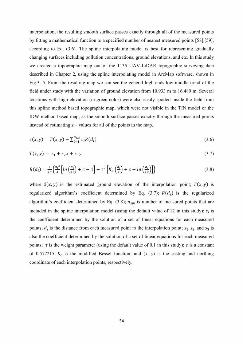
54

interpolation, the resulting smooth surface passes exactly through all of the measured points

by fitting a mathematical function to a specified number of nearest measured points [58],[59],

according to Eq. (3.6). The spline interpolating model is best for representing gradually

changing surfaces including pollution concentrations, ground elevations, and etc. In this study

we created a topographic map out of the 1135 UAV-LiDAR topographic surveying data

described in Chapter 2, using the spline interpolating model in ArcMap software, shown in

Fig.3. 5. From the resulting map we can see the general high-ends-low-middle trend of the

field under study with the variation of ground elevation from 10.933 m to 16.489 m. Several

locations with high elevation (in green color) were also easily spotted inside the field from

this spline method based topographic map, which were not visible in the TIN model or the

IDW method based map, as the smooth surface passes exactly through the measured points

instead of estimating z – values for all of the points in the map.

��(𝑥, 𝑦) = 𝑇(𝑥, 𝑦) + ∑ 𝑐𝑖𝑅(𝑑𝑖)𝑛𝑠𝑝𝑙

𝑖=1 (3.6)

𝑇(𝑥, 𝑦) = 𝑠1 + 𝑠2𝑥 + 𝑠3𝑦 (3.7)

𝑅(𝑑𝑖) =1

2𝜋{

𝑑𝑖2

4[𝑙𝑛 (

𝑑𝑖

2𝜏) + 𝑐 − 1] + 𝜏2 [𝐾𝑜 (

𝑑𝑖

𝜏) + 𝑐 + 𝑙𝑛 (

𝑑𝑖

2𝜋)]} (3.8)

where ��(𝑥, 𝑦) is the estimated ground elevation of the interpolation point; 𝑇(𝑥, 𝑦) is

regularized algorithm’s coefficient determined by Eq. (3.7); 𝑅(𝑑𝑖) is the regularized

algorithm’s coefficient determined by Eq. (3.8); 𝑛𝑠𝑝𝑙 is number of measured points that are

included in the spline interpolation model (using the default value of 12 in this study); 𝑐𝑖 is

the coefficient determined by the solution of a set of linear equations for each measured

points; 𝑑𝑖 is the distance from each measured point to the interpolation point; 𝑠1, 𝑠2, and 𝑠3 is

also the coefficient determined by the solution of a set of linear equations for each measured

points; 𝜏 is the weight parameter (using the default value of 0.1 in this study); 𝑐 is a constant

of 0.577215; 𝐾𝑜 is the modified Bessel function; and (x, y) is the easting and northing

coordinate of each interpolation points, respectively.

55

Fig.3. 5 Interpolation result using spline method

Natural neighbor interpolation model is very similar to the IDW model, except that it

determines weight parameter based on proportionate areas instead of the inversed distances,

shown in Fig.3. 6, where the red star mark represents the interpolation point and the black

dots represent the surrounding measured points. The weight parameter for each surrounding

measured point is calculated according to the proportion of overlapped areas between each

measured point’s polygon and the interpolation point’s polygon, and the polygons are

generated using Voronoi diagram [60]. The natural neighbor model only uses the closest

subset of the measured points that surround the interpolation point. Same with the spline

interpolation model, the resulting surface passes exactly through each measured point [61].

We created a topographic map using the natural neighbor interpolation model in ArcMap

software, shown in Fig.3. 7. From the resulting map we can also understand the general high-

north-low-south terrain of the field under study, with the variation of ground elevation from

13.253 m to 14.560 m. The ditch over the border of two adjacent fields was clearly

distinguished and shown in red color, whilst a short ridge inside the field was shown in

yellow color.

56

Fig.3. 6 Illustration of natural neighbor method (by Esri)

Fig.3. 7 Interpolation result using natural neighbor method

Kriging model, which is an advanced geostatistical procedure, interpolates scattered

points with z–values to create a raster surface. Whilst the above mentioned interpolation

methods including IDW, spline, or natural neighbor are solely based on the surrounding

measured points’ z–values for estimating the z–value for each interpolation point, Kriging

model is essentially different from them because it is based the geostatistical relationships

among the measured points by assuming that the spatial correlation between measured points

can be used to explain variations in the surface. Thus, in contrast with the IDW model, the

weight parameter for each surrounding measured point in the Kriging model is not only based

57

on the distance to the interpolation point but also influenced by the overall spatial

autocorrelation of the measured points, expressed as Eq. (3.9). Kriging interpolation is

originated from mineral exploration, and is very popular in geological analysis. In this study

we used the ordinary Kriging method with the spherical semivariogram model in ArcMap

software to generate a topographic map from the 1135 UAV-LiDAR system based

topographic surveying data described in Chapter 2, shown in Fig.3. 8. From the resulting

surface map we may conclude that the Kriging method based topographic map is very similar

to the IDW method based one: the general high-north-low-south trend of the ground elevation

of the field under study can be clearly observed, and a ditch (in red color) in south-north

direction could also be visualized.

��(𝑥, 𝑦) = ∑ 𝑤𝑖𝑧(𝑥𝑖 , 𝑦𝑖)𝑛𝑘𝑟𝑖𝑖=1 (3.9)

where ��(𝑥, 𝑦), 𝑛𝑘𝑟𝑖 , 𝑤𝑖, and, 𝑧(𝑥𝑖, 𝑦𝑖) is the estimated z-value of the interpolation point, the

number of measured points included in the Kriging model (using the default value of 12 in

this study), weighting factor of each measured points, and each measured point’s z -value,

respectively.

Fig.3. 8 Interpolation result using Kriging method

3.2.2 Generating Low-altitude Aerial Photogrammetric DSM

58

Aerial photogrammetric DSM is suitable for large-scale areas or mountainous areas

where it is not easy to directly measure the ground elevations. Aerial photogrammetric DSM

is also featured with good spatial resolution, and it has been reported that about 85% of

topographic maps are generated using aerial photogrammetric techniques [62]. However,

generating photogrammetric DSM from aerial photographs usually needs high-quality

arrangement of GCPs spreading uniformly around the whole area of interest. Unfortunately, it

is always impossible in practice to find enough distinguishable features both in real world as

well as aerial images to be used as GCPs in farmlands, and artificially setting up enough

markers as GCPs seems not only time-consuming but also not feasible during crop growing

season for crop height estimation. Thus, in this study we investigated the accuracy of ground

elevation values extracted from the aerial photographic DSM by comparing them with the

corresponding RTK-GPS data explained in Chapter 2.

Table 3. 1 Flight plan and camera specifications

Flight Plan Camera Specification

Altitude (above ground level, m) 80 Weight (gram) 180

Endurance (min) 2 Dimensions (cm) 12.1 * 6.6 * 4.6

Flight Range (m) 400 Camera resolution 1280 × 960 pixels

Speed (m/s) 6 Focal length (mm) 5.5

Captures 121 Sensor size(mm) 4.8 × 3.6

Tracks 2 Horizontal Field of

View (degree)

47.2

The aerial photogrammetric DSM is acquired by stitching 121 individual images based

on multi-view 3D reconstruction image processing technique in Agisoft PhotoScan software.

The RedEdge camera (MicaSense Inc., Seattle, WA, USA) was used to take these images,

which is installed on the UAV platform described in Chapter 2. The UAV-camera system

flew at about 80 m above ground level with the ground speed of about 8 m/s and the flight

track interval of 15 m. The camera captured one image per second with the spatial resolution

of about 0.05 m (5 cm). Accordingly, the forward overlap rate and the side overlap rate could

be calculated as 83% and 77%. According to the specifications for office operation of low-

altitude digital aero-photogrammetry, the minimum forward overlap rate and side overlap rate

is claimed no less than 53% and 8%, respectively, and our flight satisfies the operation

59

requirements. Four field corners were selected as GCPs in this experiment, and the geospatial

coordinates were measured by using RTK-GPS module to geo-reference the resulting

photogrammetric DSM.

The process of generating photogrammetric DSM from low-altitude aerial images was

shown in Fig.3. 9, and the resulting photogrammetric DSM is shown in Fig.3. 10. In the DSM

map four GCPs’ locations were indicated using star marks in black color, and the field of

interest was distinguished using black polylines (RTK-GPS’s trajectory). From the DSM map

we can see that the surface elevation varies from 3.86 m to 18.724 m and it does not comply

with the real world situation. We may conclude that the absolute accuracy of the field’s

surface elevation is not reliable, due to the poor capability of interpolation when the elevation

values of the features that are outside the rein of GCPs are determined. However, we may

also conclude that the low-altitude aerial photogrammetric DSM has good relative accuracy:

in the north-most area we can see the growing maize stalks (about 2 m in height) were

distinctively depicted in green color (the highest surface elevation); in the middle part of the

west-most area we can see the growing soybean stalks (about 0.8 m in height) were depicted

in yellow color (medium-high surface elevation); the harvested wheat field’s bare soil part

was shown in red color (low surface elevation); whilst the ditch (about 2 m in depth) over the

northern headland of the wheat field was shown in dark red color (the lowest surface

elevation).

Fig.3. 9 Workflow of generating photogrammetric DSM

60

Fig.3. 10 The resulting photogrammetric DSM from aerial images

3.2.3 Integrating Aerial Photogrammetric DSM with UAV-LiDAR Data

Fig.3. 11 Variations of RTK-GPS’s altitude and the corresponding DSM’s surface elevation data

A set of RTK-GPS data were used in order to evaluate the ground surface elevation

values of the resulting aerial photogrammetric DSM. The spatial distribution of RTK-GPS

samples for validation was also shown in Fig.3. 10 in bright green color. Subsequently,

61

surface elevation data which shares the same coordinates with these RTK-GPS samples were

extracted from the aerial photogrammetric DSM in ENVI software (Exelis VIS, Inc., Boulder,

CO, USA). The variations of RTK-GPS’s altitude as well as the corresponding aerial

photogrammetric DSM’s surface elevation data were shown in Fig.3. 11. From Fig.3. 11 we

may conclude that surface elevation values of the DSM samples that are near to the GCPs

have good absolute accuracy when compared with the corresponding RTK-GPS samples’

altitude, and the accuracy of DSM samples’ surface elevation values decreases as samples

deviate from the GCPs. Nonetheless, from the highly coincident tendencies of these two sets

of elevation data we may come to a conclusion that the relative accuracy between the

neighboring pixels of the aerial photogrammetric DSM is considerably good. Therefore, we

came up with a solution which utilizes the relative difference of the surface ground elevations

among the neighboring pixels of the aerial photographic DSM for integration with the UAV-

LiDAR system based topographic surveying data, described in Chapter 2, for an improved

topographic map.

This method utilizes the simple and autonomous flight of the UAV-LiDAR system and

requires only a few boundary corners to be measured as GCPs for the generation of aerial

photogrammetric DSM (usually measuring the coordinates of 4 corners of the field under

study is the minimum requirement for geo-referencing purpose). Firstly, all of the 1135

UAV-LiDAR system based topographic surveying points (shown in Fig.3. 12 as larger dots)

were defined as standard data set, denoting ( xUAVi, yUAVi, zUAVi ). Furthermore, the

georeferenced aerial photogrammetric DSM was processed using a median filter (with the

kernel size of 11) in ENVI software for such reasons: a). Adverse impact of the potential

misplaced geo-registration between each UAV-LiDAR system based topographic surveying

data and the corresponding pixel of the geo-referenced aerial photogrammetric DSM could be

compensated; b). The abnormal values of the ground surface elevations of the aerial

photogrammetric DSM could be screened out, which tend to occur during multi-view 3D

image reconstruction process due to feature mismatching, camera intrinsic malfunction, and

etc. Secondly, ground surface elevation values of the points that share the same geospatial

coordinates with the standard data set were acquired out of the median-filtered aerial

photogrammetric DSM and defined as reference data set, denoting (xUAVi, yUAVi, zDSMi ).

Thirdly, surface elevation values of the surrounding points (shown in Fig.3. 12 as smaller

dots amounting to as many as 6810 points) within the neighboring areas of the standard data

set were also acquired from the same median filtered aerial photogrammetric DSM, denoting

62

(xneighbori, yneighbori, zneighbori). Subsequently, the differences of ground surface elevation

values between each point of reference data set and its corresponding neighboring point were

calculated according to Eq. (3.15). Finally, the aerial photogrammetric DSM based surface

elevation of each surrounding point could be rectified using the corresponding UAV-LiDAR

system based topographic surveying data according to Eq. (3.16), denoting

(𝑥𝑛𝑒𝑖𝑔ℎ𝑏𝑜𝑟𝑖, 𝑦𝑛𝑒𝑖𝑔ℎ𝑏𝑜𝑟𝑖, 𝑧𝑛𝑒𝑖𝑔ℎ𝑏𝑜𝑟𝑖′ ).

∆𝑧𝑖 = 𝑧𝑛𝑒𝑖𝑔ℎ𝑏𝑜𝑟𝑖 − 𝑧𝐷𝑆𝑀𝑖 (3.15)

𝑧𝑛𝑒𝑖𝑔ℎ𝑏𝑜𝑟𝑖′ = 𝑧𝑈𝐴𝑉𝑖 + ∆𝑧𝑖 (3.16)

where 𝑧𝑛𝑒𝑖𝑔ℎ𝑏𝑜𝑟𝑖 , 𝑧𝐷𝑆𝑀𝑖 , and ∆𝑧𝑖 is the aerial photogrammetric DSM’s surface elevation

values of the surrounding points within the neighboring areas of the reference data set, the

aerial photogrammetric DSM’s surface elevation values of the reference data set, and the

difference of ground surface elevation between each point of reference data set and its

corresponding neighboring point, respectively; whilst 𝑧𝑈𝐴𝑉𝑖 and 𝑧𝑛𝑒𝑖𝑔ℎ𝑏𝑜𝑟𝑖′ is the ground

elevation value of the UAV-LiDAR system based topographic surveying points and the

rectified ground elevation values of each surrounding point.

Fig.3. 12 Improved spatial resolution of topographic surveying points

3.3 Results and Discussion

63

3.3.1 Evaluating Topographic Maps Based on Different Interpolating Methods

The accuracy of the interpolated topographic map is depending on two systems of error:

one is the measuring accuracy of each sampled points, i.e. the primitive error. As mentioned

in Chapter 2, the RSME between ground elevation value of each RTK-GPS surveying point

and the corresponding ground elevation value of the UAV-LiDAR system based topographic

surveying point was calculated as 0.035 m. Considering that the ground elevation of the field

under study varies from 13.237 m to 14.594 m according to the topographic survey data using

the UAV-LiDAR system, the RMSE is acceptable when compared with the elevation

difference of 1.357 m, which demonstrated that the primitive error of the UAV-LiDAR

topographic surveying system is minimal. The other system of error adheres to the

mathematical model of each specific interpolation method, i.e. the interpolation error.

Interpolation error is the main source that contributes to the accuracy of the resulting

topographic surface map, as the z–value of each interpolation point is not only determined by

the surrounding measured points’ z–values but also influenced by the neighboring measured

points’ spatial distribution, density, and etc.

Table 3. 2 Samples for evaluating accuracy of each interpolation method (in part)

Sample

Numbe

r

Geo-spatial coordinates Ground elevation (m)

Easting Northing RTK-

GPS

TIN IDW Kriging Spline Natural

Neighbo

r 1 527314.13

0

4769057.87

0

13.689 13.643 13.731 13.723 15.285 13.642

2 527315.63

0

4769062.87

0

13.645 13.598 13.570 13.573 14.683 13.597

3 527313.14

2

4769066.34

3

13.613 13.606 13.595 13.594 14.675 13.603

4 527308.13

0

4769066.87

0

13.558 13.581 13.676 13.669 13.335 13.655

5 527316.98

2

4769067.10

6

13.653 13.658 13.595 13.582 13.737 13.583

… … … … … … … … …

48 527252.63

0

4769166.87

0

13.875 13.921 13.917 13.916 13.924 13.994

49 527251.29

4

4769168.51

8

13.889 13.942 13.940 13.944 13.943 13.946

50 527244.13

0

4769176.37

0

13.852 14.142 13.982 14.030 14.224 14.142

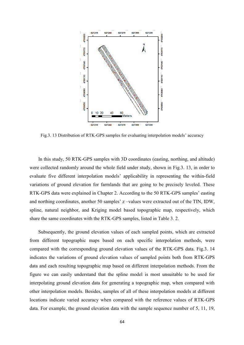
64

Fig.3. 13 Distribution of RTK-GPS samples for evaluating interpolation models’ accuracy

In this study, 50 RTK-GPS samples with 3D coordinates (easting, northing, and altitude)

were collected randomly around the whole field under study, shown in Fig.3. 13, in order to

evaluate five different interpolation models’ applicability in representing the within-field

variations of ground elevation for farmlands that are going to be precisely leveled. These

RTK-GPS data were explained in Chapter 2. According to the 50 RTK-GPS samples’ easting

and northing coordinates, another 50 samples’ z –values were extracted out of the TIN, IDW,

spline, natural neighbor, and Kriging model based topographic map, respectively, which

share the same coordinates with the RTK-GPS samples, listed in Table 3. 2.

Subsequently, the ground elevation values of each sampled points, which are extracted

from different topographic maps based on each specific interpolation methods, were

compared with the corresponding ground elevation values of the RTK-GPS data. Fig.3. 14

indicates the variations of ground elevation values of sampled points both from RTK-GPS

data and each resulting topographic map based on different interpolation methods. From the

figure we can easily understand that the spline model is most unsuitable to be used for

interpolating ground elevation data for generating a topographic map, when compared with

other interpolation models. Besides, samples of all of these interpolation models at different

locations indicate varied accuracy when compared with the reference values of RTK-GPS

data. For example, the ground elevation data with the sample sequence number of 5, 11, 19,

65

20, 21, 26, 27, 38, 42, 44, and 49 of all these five interpolation models have quite good

accuracy when compared with the reference values of RTK-GPS data; however, ground

elevation data with other sequence numbers deviate badly from the corresponding RTK-GPS

data in one interpolation model or another.

Fig.3. 14 Variations of sampled ground elevation of RTK-GPS data and topographic maps

Finally, the accuracy of each topographic surface map based on different interpolation

models is quantitatively analyzed by calculating the RMSEs between the reference ground

elevation values of RTK-GPS data and the interpolated ground elevation values of each

resulting topographic maps by using TIN model, IDW model, spline model, natural neighbor

model, and Kriging model, respectively, according to Eq. (3.10) ~ Eq. (3.14). And the results

are as follows: RMSETIN = 0.137m, RMSEIDW = 0.158 m, RMSEspl = 0.388m, RMSEnat =

0.139 m, and RMSEKri = 0.160 m, respectively. We may conclude that the TIN model is the

most suitable interpolation model for the study of representing within-field variations of

ground elevation by using UAV-LiDAR topographic surveying data, whilst the other four

interpolation models have relatively poor capability of interpolating UAV-LiDAR data for

generating a topographic map of a farmland.

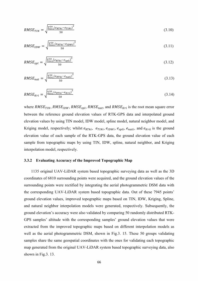
66

𝑅𝑀𝑆𝐸𝑇𝐼𝑁 = √∑ (𝑒𝑅𝑇𝑘𝑖−𝑒𝑇𝐼𝑁𝑖)50𝑖=1

2

50 (3.10)

𝑅𝑀𝑆𝐸𝐼𝐷𝑊 = √∑ (𝑒𝑅𝑇𝑘𝑖−𝑒𝐼𝐷𝑊𝑖)50𝑖=1

2

50 (3.11)

𝑅𝑀𝑆𝐸𝑠𝑝𝑙 = √∑ (𝑒𝑅𝑇𝑘𝑖−𝑒𝑠𝑝𝑙𝑖)50𝑖=1

2

50 (3.12)

𝑅𝑀𝑆𝐸𝑛𝑎𝑡 = √∑ (𝑒𝑅𝑇𝑘𝑖−𝑒𝑛𝑎𝑡𝑖)50𝑖=1

2

50 (3.13)

𝑅𝑀𝑆𝐸𝐾𝑟𝑖 = √∑ (𝑒𝑅𝑇𝑘𝑖−𝑒𝐾𝑟𝑖𝑖)50𝑖=1

2

50 (3.14)

where 𝑅𝑀𝑆𝐸𝑇𝐼𝑁, 𝑅𝑀𝑆𝐸𝐼𝐷𝑊, 𝑅𝑀𝑆𝐸𝑠𝑝𝑙, 𝑅𝑀𝑆𝐸𝑛𝑎𝑡, and 𝑅𝑀𝑆𝐸𝐾𝑟𝑖 is the root mean square error

between the reference ground elevation values of RTK-GPS data and interpolated ground

elevation values by using TIN model, IDW model, spline model, natural neighbor model, and

Kriging model, respectively; whilst 𝑒𝑅𝑇𝑘𝑖, 𝑒𝑇𝐼𝑁𝑖, 𝑒𝐼𝐷𝑊𝑖, 𝑒𝑠𝑝𝑙𝑖, 𝑒𝑛𝑎𝑡𝑖, and 𝑒𝐾𝑟𝑖𝑖 is the ground

elevation value of each sample of the RTK-GPS data, the ground elevation value of each

sample from topographic maps by using TIN, IDW, spline, natural neighbor, and Kriging

interpolation model, respectively.

3.3.2 Evaluating Accuracy of the Improved Topographic Map

1135 original UAV-LiDAR system based topographic surveying data as well as the 3D

coordinates of 6810 surrounding points were acquired, and the ground elevation values of the

surrounding points were rectified by integrating the aerial photogrammetric DSM data with

the corresponding UAV-LiDAR system based topographic data. Out of these 7945 points’

ground elevation values, improved topographic maps based on TIN, IDW, Kriging, Spline,

and natural neighbor interpolation models were generated, respectively. Subsequently, the

ground elevation’s accuracy were also validated by comparing 50 randomly distributed RTK-

GPS samples’ altitude with the corresponding samples’ ground elevation values that were

extracted from the improved topographic maps based on different interpolation models as

well as the aerial photogrammetric DSM, shown in Fig.3. 15. These 50 groups validating

samples share the same geospatial coordinates with the ones for validating each topographic

map generated from the original UAV-LiDAR system based topographic surveying data, also

shown in Fig.3. 13.

67

From Fig.3. 15 we may conclude that the sampled ground elevation values of the aerial

photogrammetric DSM have the smoothest tendency; however, it also expressed the most

deviated situation from the corresponding reference RTK-GPS data; and same with situation

in Fig.3. 14 spline interpolation model is still most unsuitable to be used for interpolating

ground elevation data for generating a topographic map of a farmland due to a wide range of

fluctuation. Besides, samples of all of these interpolation models for the improved

topographic maps at different locations indicate varied accuracy when compared with the

corresponding altitude values of RTK-GPS data. The ground elevation data with the sample

sequence number of 5, 8, 11, 19, 20, 21, 26, 27, 28, 29, 34, 35, 36, 38, 41, 42, 44, 47, 48, and

49 of all these five interpolation models have very good accuracy when compared with the

corresponding altitude values of RTK-GPS data; and the overall accuracy of ground elevation

values of most samples of these different improved topographic maps was improved by a

large extent. The ground elevation’s accuracy of the resulting aerial photogrammetric DSM,

as explained in Sec.3.2.3, is good when the sample is near to the location of GCPs and

deteriorates as the distance from the sample to the location of GCPs increases.

Fig.3. 15 Variations of sampled ground elevation of RTK-GPS data and improved topographic maps

as well as the aerial photographic DSM

68

Table 3. 3 Samples for evaluating accuracies of the aerial photogrammetric DSM and the

improved topographic maps (in part)

Sample

Numbe

r

Ground elevation (m)

RTK-

GPS

Improved

TIN

Improved

IDW

Improved

Kriging

Improved

Spline

Improved Natural

Neighbor

Aerial

DSM

1 13.689 13.685 13.694 13.691 13.586 13.677 13.527

2 13.645 13.603 13.670 13.665 12.218 13.605 13.466

3 13.613 13.658 13.598 13.600 12.823 13.621 13.398

4 13.558 13.657 13.678 13.672 13.681 13.674 13.345

5 13.653 13.602 13.589 13.588 13.599 13.587 13.394

… … … … … … … …

48 13.875 13.914 13.919 13.932 13.921 13.914 13.863

49 13.889 13.927 13.939 13.919 13.937 13.937 13.892

50 13.852 13.930 14.071 14.177 13.847 13.976 13.927

The ground elevation values extracted from the improved topographic maps based on

different interpolation models as well as the aerial photogrammetric DSM and the

corresponding RTK-GPS altitude data were, in part, listed in Table 3. 3. And accordingly the

RMSEs between each sample’s RTK-GPS altitude and the corresponding samples’ ground

elevation value extracted from the improved topographic maps as well as the aerial

photogrammetric DSM were calculated, respectively, according to Eq. (3.15)~ Eq. (3.20).

𝑅𝑀𝑆𝐸𝑖𝑚𝑝𝑇𝐼𝑁 = √∑ (𝑒𝑅𝑇𝑘𝑖−𝑒𝑖𝑚𝑝𝑇𝐼𝑁𝑖)50𝑖=1

2

50 (3.15)

𝑅𝑀𝑆𝐸𝑖𝑚𝑝𝐼𝐷𝑊 = √∑ (𝑒𝑅𝑇𝑘𝑖−𝑒𝑖𝑚𝑝𝐼𝐷𝑊𝑖)50𝑖=1

2

50 (3.16)

𝑅𝑀𝑆𝐸𝑖𝑚𝑝𝑠𝑝𝑙 = √∑ (𝑒𝑅𝑇𝑘𝑖−𝑒𝑖𝑚𝑝𝑠𝑝𝑙𝑖)50𝑖=1

2

50 (3.17)

𝑅𝑀𝑆𝐸𝑖𝑚𝑝𝑛𝑎𝑡 = √∑ (𝑒𝑅𝑇𝑘𝑖−𝑒𝑖𝑚𝑝𝑛𝑎𝑡𝑖)50𝑖=1

2

50 (3.18)

69

𝑅𝑀𝑆𝐸𝑖𝑚𝑝𝐾𝑟𝑖 = √∑ (𝑒𝑅𝑇𝑘𝑖−𝑒𝑖𝑚𝑝𝐾𝑟𝑖𝑖)50𝑖=1

2

50 (3.19)

𝑅𝑀𝑆𝐸𝐷𝑆𝑀 = √∑ (𝑒𝑅𝑇𝑘𝑖−𝑒𝐷𝑆𝑀𝑖)50𝑖=1

2

50 (3.20)

where 𝑅𝑀𝑆𝐸𝑖𝑚𝑝𝑇𝐼𝑁, 𝑅𝑀𝑆𝐸𝑖𝑚𝑝𝐼𝐷𝑊, 𝑅𝑀𝑆𝐸𝑖𝑚𝑝𝑠𝑝𝑙 , 𝑅𝑀𝑆𝐸𝑖𝑚𝑝𝑛𝑎𝑡 , 𝑅𝑀𝑆𝐸𝑖𝑚𝑝𝐾𝑟𝑖 , and 𝑅𝑀𝑆𝐸𝐷𝑆𝑀

is the root mean square error between each sample’s RTK-GPS altitude and the

corresponding ground elevation value extracted from the improved topographic maps by

using TIN, IDW, spline, natural neighbor, and Kriging interpolation model, respectively, as

well as the aerial photogrammetric DSM; whilst 𝑒𝑅𝑇𝑘𝑖, 𝑒𝑖𝑚𝑝𝑇𝐼𝑁𝑖, 𝑒𝑖𝑚𝑝𝐼𝐷𝑊𝑖, 𝑒𝑖𝑚𝑝𝑠𝑝𝑙𝑖, 𝑒𝑖𝑚𝑝𝑛𝑎𝑡𝑖,

𝑒𝑖𝑚𝑝𝐾𝑟𝑖𝑖, and 𝑒𝐷𝑆𝑀𝑖 is the ground elevation value of each sample of the RTK-GPS data, the

ground elevation values of each sample from improved topographic maps by using TIN, IDW,

spline, natural neighbor, and Kriging interpolation model, respectively, as well as the aerial

photogrammetric DSM.

As a result, RMSEimpTIN , RMSEimpIDW , RMSEimpspl , RMSEimpnat , RMSEimpKri , and

RMSEDSM was calculated as 0.059 m, 0.118 m, 0.258 m, 0.107 m, 0.127 m, and 0.197,

respectively. In comparison, the RSMEs between the same sets of RTK-GPS data with the

corresponding ground elevation values that are extracted from the resulting topographic maps

generated from the original 1135 sets of topographic surveying data of the UAV-LiDAR

system based on different interpolation models have already been calculated in Sec. 3.3.1 as

follows: RMSETIN = 0.137 m , RMSEIDW = 0.158 m , RMSEspl = 0.388 m , RMSEnat =

0.139 m , and RMSEKri = 0.160 m , respectively. Hereby we may conclude that the

integration of aerial photogrammetric DSM data with the topographic surveying data based

on the UAV-LiDAR system has distinctive benefits on improving the accuracy of each

interpolated topographic map, and the improved topographic map based on TIN interpolation

model has the best accuracy with the RSME of 0.059 m (5.9 cm).

The resulting topographic map generated from the integrated surveying data and based

on the TIN interpolation model was shown in Fig.3. 16, from which we can clearly recognize

the general high-north-low-south terrain of the field under study, and a long ditch over the

west border of two adjacent fields in south-north direction could also be observed.

Furthermore, the detailed fluctuation of ground elevation inside the field was much more

obvious in this improved topographic map due to high spatially intensive measured points

70

(with the spatial resolution of about 1 m * 0.5 m), in comparison with the topographic map

generated from the original UAV-LiDAR surveying points (with the resolution of about 6 m

* 0.5 m). We may also see two deep puddles marked in black circle and rectangle in both

Fig.3. 16 (the dark red areas) and Fig.3. 17 (the vegetative green area). Due to the relatively

low ground elevation of these two puddles, wheat plants were drown (crop failure) during the

growing season when precipitation is concentrative in October and snowmelt water

converges in April. As the wheat plants die, weed ensues in the following days to cause

further yield loss, shown in Fig.3. 17.

Fig.3. 16 Improved topographic maps using TIN interpolation method

Fig.3. 17 Actual field condition of wheat (two days prior to harvesting)

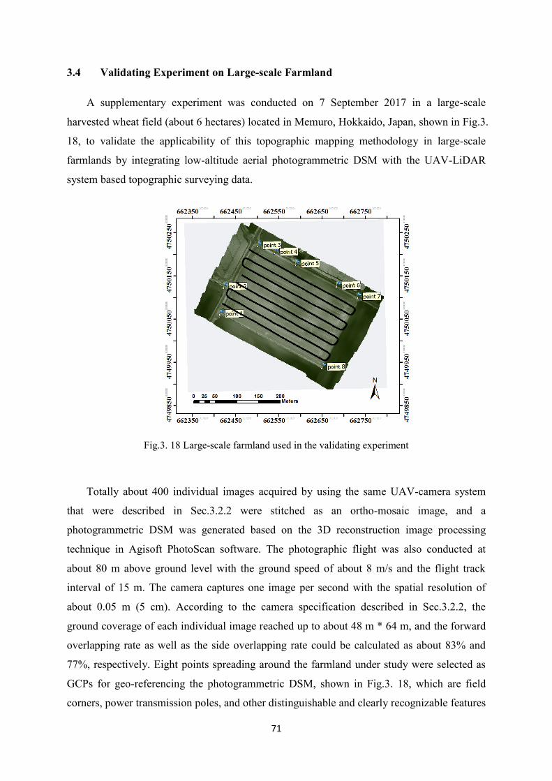
71

3.4 Validating Experiment on Large-scale Farmland

A supplementary experiment was conducted on 7 September 2017 in a large-scale

harvested wheat field (about 6 hectares) located in Memuro, Hokkaido, Japan, shown in Fig.3.

18, to validate the applicability of this topographic mapping methodology in large-scale

farmlands by integrating low-altitude aerial photogrammetric DSM with the UAV-LiDAR

system based topographic surveying data.

Fig.3. 18 Large-scale farmland used in the validating experiment

Totally about 400 individual images acquired by using the same UAV-camera system

that were described in Sec.3.2.2 were stitched as an ortho-mosaic image, and a

photogrammetric DSM was generated based on the 3D reconstruction image processing

technique in Agisoft PhotoScan software. The photographic flight was also conducted at

about 80 m above ground level with the ground speed of about 8 m/s and the flight track

interval of 15 m. The camera captures one image per second with the spatial resolution of

about 0.05 m (5 cm). According to the camera specification described in Sec.3.2.2, the

ground coverage of each individual image reached up to about 48 m * 64 m, and the forward

overlapping rate as well as the side overlapping rate could be calculated as about 83% and

77%, respectively. Eight points spreading around the farmland under study were selected as

GCPs for geo-referencing the photogrammetric DSM, shown in Fig.3. 18, which are field

corners, power transmission poles, and other distinguishable and clearly recognizable features

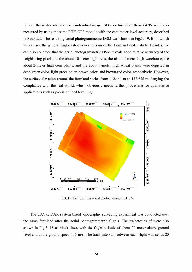
72

in both the real-world and each individual image. 3D coordinates of these GCPs were also

measured by using the same RTK-GPS module with the centimeter-level accuracy, described

in Sec.3.2.2. The resulting aerial photogrammetric DSM was shown in Fig.3. 19, from which

we can see the general high-east-low-west terrain of the farmland under study. Besides, we

can also conclude that the aerial photogrammetric DSM reveals good relative accuracy of the

neighboring pixels, as the about 10-meter high trees, the about 5-meter high warehouse, the

about 2-meter high corn plants, and the about 1-meter high wheat plants were depicted in

deep green color, light green color, brown color, and brown-red color, respectively. However,

the surface elevation around the farmland varies from 112.441 m to 137.625 m, denying the

compliance with the real world, which obviously needs further processing for quantitative

applications such as precision land levelling.

Fig.3. 19 The resulting aerial photogrammetric DSM

The UAV-LiDAR system based topographic surveying experiment was conducted over

the same farmland after the aerial photogrammetric flights. The trajectories of were also

shown in Fig.3. 18 as black lines, with the flight altitude of about 30 meter above ground

level and at the ground speed of 5 m/s. The track intervals between each flight was set as 20

73

meters for large coverage, and the UAV-LiDAR system based topographic surveying points’

spatial resolution could be accordingly calculated as 20 m * 0.5 m, described in Sec.2.3.1.

We removed the samples during the process of taking off, turning around, and landing of

the UAV-LiDAR topographic surveying system, and totally 3889 sets of effective sample

data were acquired. Using TIN interpolation method, a topographic map was generated based

on these 3889 original UAV-LiDAR system’s topographic surveying data, shown in Fig.3. 20.

From Fig.3. 20 we may also conclude that the farmland under study has the same general

high-east-low-west terrain feature with the one of the aerial photogrammetric DSM, and the

ground surface elevation varies from 112.944 m to 118.818 m. With a heavy change in

elevation of about 6 meters, this farmland desperately needs land forming operation in order

to achieve optimal crop growth status and yield. For example, dividing this large-scale

farmland into several terraced sub-zones and then implementing precision land leveling

operation would be advisable, so that the fertile top soils over the high ground elevation area

could be preserved to the maximum extent.

Fig.3. 20 The resulting topographic map based on TIN interpolation method using UAV-LiDAR

system based topographic surveying data

We have already discussed in Chapter 2 that the poor spatial resolution of topographic

surveying points influences the overall accuracy as well as the capability of demonstrating

74

the detailed features in an interpolated topographic map. In this section we are to evaluate the

applicability of generating a topographic map by integrating ground elevation values of an

aerial photogrammetric DSM with the topographic surveying data based on the UAV-LiDAR

system for large-scale farmland.

Firstly, the spatial resolution of topographic surveying points was improved to about 1 m

* 0.5 m from about 20 m* 0.5 m using the same methodology explained in Sec.3.2.3, shown

in Fig.3. 21: the larger dots are the original topographic surveying data based on UAV-

LiDAR system, whilst the smaller ones are neighboring samples whose ground elevation

values are rectified using the same methodology explained in Sec.3.2.3. Subsequently, all of

these original topographic surveying data based on the UAV-LiDAR system and the rectified

neighboring samples were included to generate an improved topographic map using TIN

interpolation model, and the resulting map was shown Fig.3. 22.

Fig.3. 21 Spatial distribution of topographic surveying data in large-scale farmland

From Fig.3. 22 we can conclude that the improved topographic map demonstrates much

more detailed terrain information of the farmland under study than the former one that was

merely based on the UAV-LiDAR system’s topographic data, shown in Fig.3. 20, with the

general high-east-low-west terrain and ground elevation’s variation from 112.806 m to

119.098 m. Two large and several small puddles could also be spotted at the west most part

75

and in the middle part of the field, shown in red and dark yellow color, which poses potential

threat to the healthy growth as well as yield of crops due to stagnant water and high humidity.

Fig.3. 22 The resulting topographic map by integrating aerial photogrammetric DSM and UAV-

LiDAR system based topographic surveying data

Table 3. 4 Samples for evaluating accuracy of each interpolation method (in part)

Sample

Number

Geo-spatial coordinates Ground elevation (m)

Easting Northing PPK-

GPS

Aerial

DSM

Topographic

Map

Improved

Topographic

Map 1 527314.13

0

4769057.87

0

114.165 114.264 113.908 113.939

2 527315.63

0

4769062.87

0

114.643 113.727 114.515 114.679

3 527313.14

2

4769066.34

3

114.213 113.839 114.360 114.439

4 527308.13

0

4769066.87

0

114.205 113.895 114.000 114.051

5 527316.98

2

4769067.10

6

114.134 113.978 114.085 114.032

… … … … … … …

18 662654.36

9

4750021.11

8

117.688 116.480 117.676 117.652

19 662665.97

6

4750049.94

9

117.838 116.648 117.900 117.864

20 662677.91

7

4750077.74

5

117.436 116.625 117.623 117.557

76

Fig.3. 23 PPK-GPS samples’ spatial distribution

Finally, 20 samples’ 3D coordinates were measured by using the handheld PPK-GPS

module with the centimeter-level accuracy, explained in Sec.2.4.1. The coordinates of these

samples were listed in Table 3. 4, and the spatial distributions were shown in Fig.3. 23.

Accordingly, ground elevation values of the aerial photogrammetric DSM, the topographic

map based on TIN interpolation model using the original UAV-LiDAR system’s topographic

surveying data, and the improved topographic map based on TIN interpolation model by

integrating the UAV-LiDAR system’s topographic surveying data and the aerial

photogrammetric DSM data of these samples were extracted, respectively. The ground

elevation values of different models were also listed in Table 3. 4, and RMSEs of sampled

ground elevation data between the improved topographic map based on the UAV-LiDAR

system’s topographic surveying data and the aerial photogrammetric DSM, the topographic

map based on the original UAV-LiDAR system’s topographic surveying data, the aerial

photogrammetric DSM, and the corresponding PPK-GPS’s altitude was calculated according

to Eq. (3.21) to Eq. (3.23). As the result, RMSEDSMlar, RMSETINlar, and RMSEImpTINlar was

calculated as 1.040 m, 0.468 m, and 0.132 m, respectively. And we may conclude that the

methodology of integrating UAV-LiDAR system based topographic surveying data with the

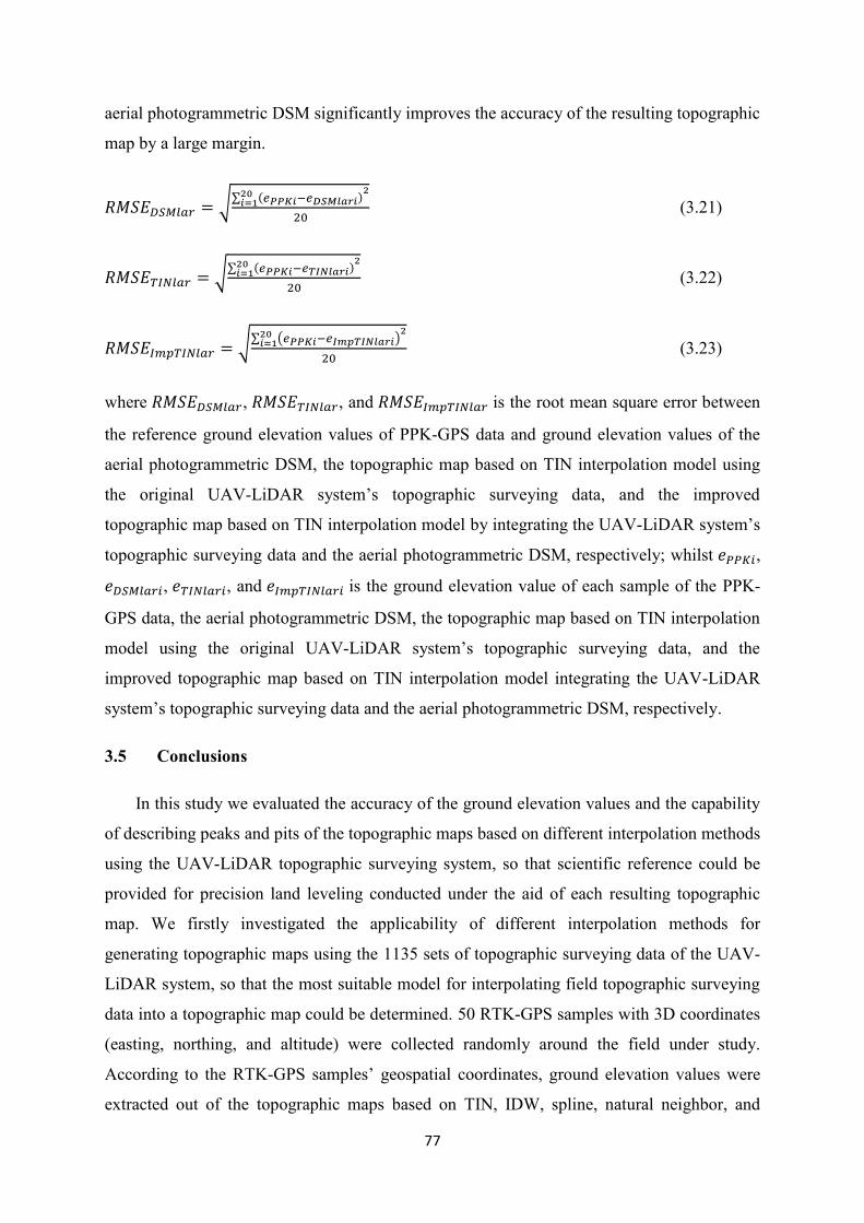
77

aerial photogrammetric DSM significantly improves the accuracy of the resulting topographic

map by a large margin.

𝑅𝑀𝑆𝐸𝐷𝑆𝑀𝑙𝑎𝑟 = √∑ (𝑒𝑃𝑃𝐾𝑖−𝑒𝐷𝑆𝑀𝑙𝑎𝑟𝑖)20𝑖=1

2

20 (3.21)

𝑅𝑀𝑆𝐸𝑇𝐼𝑁𝑙𝑎𝑟 = √∑ (𝑒𝑃𝑃𝐾𝑖−𝑒𝑇𝐼𝑁𝑙𝑎𝑟𝑖)20𝑖=1

2

20 (3.22)

𝑅𝑀𝑆𝐸𝐼𝑚𝑝𝑇𝐼𝑁𝑙𝑎𝑟 = √∑ (𝑒𝑃𝑃𝐾𝑖−𝑒𝐼𝑚𝑝𝑇𝐼𝑁𝑙𝑎𝑟𝑖)20𝑖=1

2

20 (3.23)

where 𝑅𝑀𝑆𝐸𝐷𝑆𝑀𝑙𝑎𝑟, 𝑅𝑀𝑆𝐸𝑇𝐼𝑁𝑙𝑎𝑟, and 𝑅𝑀𝑆𝐸𝐼𝑚𝑝𝑇𝐼𝑁𝑙𝑎𝑟 is the root mean square error between

the reference ground elevation values of PPK-GPS data and ground elevation values of the

aerial photogrammetric DSM, the topographic map based on TIN interpolation model using

the original UAV-LiDAR system’s topographic surveying data, and the improved

topographic map based on TIN interpolation model by integrating the UAV-LiDAR system’s

topographic surveying data and the aerial photogrammetric DSM, respectively; whilst 𝑒𝑃𝑃𝐾𝑖,

𝑒𝐷𝑆𝑀𝑙𝑎𝑟𝑖, 𝑒𝑇𝐼𝑁𝑙𝑎𝑟𝑖, and 𝑒𝐼𝑚𝑝𝑇𝐼𝑁𝑙𝑎𝑟𝑖 is the ground elevation value of each sample of the PPK-

GPS data, the aerial photogrammetric DSM, the topographic map based on TIN interpolation

model using the original UAV-LiDAR system’s topographic surveying data, and the

improved topographic map based on TIN interpolation model integrating the UAV-LiDAR

system’s topographic surveying data and the aerial photogrammetric DSM, respectively.

3.5 Conclusions

In this study we evaluated the accuracy of the ground elevation values and the capability

of describing peaks and pits of the topographic maps based on different interpolation methods

using the UAV-LiDAR topographic surveying system, so that scientific reference could be

provided for precision land leveling conducted under the aid of each resulting topographic

map. We firstly investigated the applicability of different interpolation methods for

generating topographic maps using the 1135 sets of topographic surveying data of the UAV-

LiDAR system, so that the most suitable model for interpolating field topographic surveying

data into a topographic map could be determined. 50 RTK-GPS samples with 3D coordinates

(easting, northing, and altitude) were collected randomly around the field under study.

According to the RTK-GPS samples’ geospatial coordinates, ground elevation values were

extracted out of the topographic maps based on TIN, IDW, spline, natural neighbor, and

78

Kriging model, respectively. And we can understand that the spline interpolation model is

most unsuitable to be used for interpolating ground elevation data for generating a

topographic map, whilst the topographic map based on the TIN interpolation model is the

most accurate one.

From the resulting topographic map based on the TIN interpolation model, we can see

clearly that the field has a high-north-low-south trend in elevation varying from 13.237 m to

14.552 m; besides, we can also visualize a distinguishing ridge in south-north direction as

well as a line of ditch in south-north direction within the field. According to field survey we

confirmed that the ditch in south-north direction coincides with the border of two adjacent

fields with relatively low ground elevation, where large area of wheat plants were drown to

death and weeds spring up during the ripening growth stage of wheat. RMSE between the

sampled reference altitude values of RTK-GPS data and the corresponding ground elevation

values of the resulting topographic map based on TIN interpolation model was calculated as

0.137 m, which is not ideal but acceptable in consideration of the field’s elevation change of

about 1.4 m.

Then an aerial photogrammetric DSM model of the same field was created based on

multi-view image processing techniques after acquiring digital images from a UAV-camera

system. Ground elevation values were extracted out of the aerial photogrammetric DSM,

which share the same geospatial coordinates with the original UAV-LiDAR system based

topographic surveying data as well as the corresponding neighboring pixels. In this way, the

spatial resolution of the surveying points was improved from about 6 m * 0.5 m to about 1 m

* 0.5 m, as the spatial density of the surveying points also plays a paramount role in

generating an accurate topographic map by using interpolation methods. Afterwards, the

samples’ ground elevation values of the aerial photogrammetric DSM were rectified and

improved topographic maps were generated based on the totally 7945 sets of samples’ ground

elevation values using TIN, IDW, Kriging, Spline, and natural neighbor interpolation models,

respectively. Accuracies of the improved topographic maps were also validated by

calculating RMSEs between RTK-GPS samples’ altitude and the corresponding samples’

ground elevation values that were extracted from the improved topographic maps based on

different interpolation models. We may conclude that the overall accuracy of each improved

topographic map was improved by a large extent when compared with the accuracy of the

corresponding topographic map generated by only using the original UAV-LiDAR system’s

79

topographic surveying data. And still, TIN interpolation model expressed best performance

when used to generate an improved topographic map based on the integrated data of aerial

photogrammetric DSM and the original UAV-LiDAR system’s topographic surveying data.

The RSME between the RTK-GPS altitude and the corresponding ground elevation values of

the improved topographic map based on TIN interpolation model was calculated as 0.059 m

(5.9 cm), due to high spatially intensive interpolated points with the spatial resolution of

about 1 m * 0.5 m. The accurate improved topographic map confirmed the feasibility of

conducting topographic survey for farmlands by using the simple and efficient UAV-LiDAR

system in combination with the low-altitude aerial photogrammetric flights.

Finally, we also experimentally validated the accuracy as well as feasibility of using such

a topographic surveying outfit in a large-scale farmland, by changing the cross-track interval

of the UAV-LiDAR topographic surveying flights from about 6 meters to about 20 meters for

large coverage. We improved the spatial resolution of the interpolation points from about 20

m * 0.5 m to about 1 m * 0.5 m by integrating the original UAV-LiDAR system’s

topographic surveying data and the aerial photogrammetric DSM data, and an improved

topographic map was generated using TIN interpolation model. We may conclude that the

methodology of integrating UAV-LiDAR system based topographic surveying data with the

aerial photogrammetric DSM significantly improves the accuracy of the resulting topographic

map in large-scale farmland as well, when compared with the accuracies of the resulting

topographic map solely using the UAV-LiDAR system’s topographic surveying data and the

photogrammetric DSM. The RMSE between the ground elevations of the improved

topographic map, the original topographic map, as well as the aerial photogrammetric DSM,

and the corresponding PPK-GPS’s altitude was calculated as 0.132 m, 0.468 m, and 1.040 m,

respectively. In consideration that the field is featured with a ground elevation change of

about 6 m, we may conclude that the proposed methodology of generating topographic maps

for precision land leveling by integrating UAV-LiDAR system based topographic surveying

data with the low-altitude aerial photogrammetric DSM is of high practical values.

80

Chapter 4 Mapping within-Field Variations of Wheat Stalk Density

4.1 Introduction

Wheat (Triticum Spp., or Triticum Aestivum L.), a self-pollinate staple crop, has been

amongst the first domesticated food crops and the most produced cereal grains for over 8000

years in human civilization. In 2009 the global wheat production reached about 680 million

tons and in 2016 global production of wheat increased up to 749 million tons, which made it

the second most-produced cereal grain after maize [63]. The demand of wheat from global

market is still expending [64], as wheat is the leading source of vegetal protein due to its

unique major component of gluten and also a rich source of multiple kinds of essential

mineral nutrients. Wheat flour contains rather high protein content (about 13% and the value

varies among different strains and varieties) when compared with other major cereal crops

such as maize and rice, and world trade in wheat alone is greater than for all other crops

combined [65].

In general it is divided into spring wheat and winter wheat even though the cultivation of

wheat widespread over a vast geographical area all over the globe, according to flowering

responses to cold temperatures. Spring wheat is normally sowed at early spring, which needs

110 to 130 days to complete vegetative growth and reproductive growth from sowing to

harvesting, varying upon seed strain, climate, and soil conditions. On the other hand, winter

wheat is usually sowed in the autumn to germinate and grow into a young plant which stays

in a state of dormancy during winter time when temperature falls below 0 – 5 Celsius degree

and resumes vegetative growth in early spring. The growth cycle of wheat includes

germination, seedling establishment, tillering, stem elongation, heading, flowering, grain

filling, ripening, and maturity. Detailed understanding of wheat growth status during each

development stage is vital for optimal wheat field management operations. Several existing

systems to identify wheat development stages are available, with Zadoks scale being the most

widely used. Zadoks scale is a standard system which describes successive development

stages reached by the crop during each agricultural season [66]. According to Zadoks scale,

wheat development stages are generally divided into 10 distinct growth stages and of each

specific growth stage, three to dozens of sub-stages are further identified with two-digits from

00 to 99 [67], shown in Fig.4. 1.

81

Fig.4. 1 Wheat development stages (illustration of Nick Poole, FAR)

Necessary operations such as herbicides and insecticides spraying as well as nitrogenous

topdressing (for example urea solution) should be implemented timely, as different rate of

nitrogenous topdressings, herbicides, and fungicides are typically applied only at specific

stages during the wheat growth cycle. In order to optimize wheat yield and grain quality,

especially in terms of protein content that varies significantly depending on different

agricultural practices, field management in accordance with the specific growth situation of

each wheat development stage is critical. For instance, the nitrogenous topdressings are

advisable at the rate of 40~60 kg/ha during tillering stage (GS 20~29) so that the process of

tillering could be stimulated and adequacy of stalks (or stalk density) could be guaranteed for

enough wheat ears and thus the high yield. On the other hand, the nitrogenous topdressing

rate of 20~30 kg/ha during the booting stage (GS 40~49) could boost grain weight and also

grain protein content. Furthermore, recent studies on canopy management showed that not

only spring fertilizer rate but timing of fertilization also should be tailored to achieve desired

82

canopy sizes at specific development phases, which means if the wheat stalk density is too

low around the beginning of tillering stage, nitrogenous topdressing timing should be brought

forward with a higher rate in order to boost the total number of stalks. Therefore, real time

monitoring of actual wheat growth status throughout these several specific stages is of vital

importance in helping wheat growers with field management decision making.

For many years, stalk counting has been used around the world as an empirical method

of roughly estimating wheat stalk densities and understanding wheat growth status at early

growth stages. Randy Weisz et al. developed a model for decision making related to wheat

stalk densities before growth stage 30 [68], which was described as Eq. (3.1). According to

the calculation, suggestions on different rates of nitrogenous topdressing could be proposed.

Although it is feasible in case of small-scale wheat fields, this method is not suitable for large

farmlands due to the time-consuming manual sampling operation. Besides, point-source

information acquired through manually calculated stalk densities usually cannot accurately

reflect the actual spatial-variated growth status even within small-scaled farmlands. On the

other hand, remote sensing has been successfully used as an effective alternative for data

collection in applications of precision agriculture through analysis of digitalized numbers of

different bands of image data, or more often, of various kinds of vegetation indices calculated

from the reflectance or radiance of specific bands [69]. Multi-spectral satellite imagery of

visible and near infrared portions of the spectrum has been applied into detecting vegetation

areas, monitoring crop growth status, and estimating crop yield, et al., in large scale. Whilst

airborne remote sensing has been introduced into medium-scale agricultural application as a

supplementary method and often carried out as one-time operations, which employs airplane

or balloon as the carrier flying at the height of from less than 5,000m to 20,000m, and uses

digital photography with sub-meter spatial resolution. Near-ground remote sensing is often

referred to frame-based or pillar-based applications in the past, and recently the cutting edge

application of small fixed-and/or rotary-wing UAVs used in small-scale and experimental

field for spatial sampling or mapping for variable-rate operations has soared in the field of

precision agriculture.

d = (t×4) / w (4.1)

where d denotes the number of stalks per square meter, t denotes stalks per meter of row, and

w denotes row width in meter.

83

Aerial photography has been used to monitor crop growth status since 1950s by using

color or color-infrared cameras, but it is not until the start of the 21st century that widespread

applications of UAVs occurred in agricultural precision management when aerial imagery

using UAVs can be acquired more cost-effectively, with increasing spatial resolution due to

low-altitude flight capacity, and with greater safety than manned aircraft [70]-[74]. Wang [75]

et al. successfully differentiated vegetation areas from non-vegetation areas by analyzing

color images acquired from a UAV; Rasmussen [76] et al investigated four different

vegetation indices acquired from a color camera and a color-infrared camera by using both a

fixed-wing UAV and a rotary-wing UAV, and concluded that vegetation indices based on

UAV imagery have the same ability to quantify crop responses with ground-based recordings.

In this study, we are to acquire aerial digital photographs by using an agricultural digital

camera (ADC) mounted on the low-altitude UAV platform; and subsequently estimate the

within-field spatial variations of wheat stalk density from the aerial images in a less time-

consuming and accurate manner, so that suggestions on variable-rate nitrogenous topdressing

could be accordingly recommended.

4.2 Methodology

Fig.4. 2 Proposed approach of using UAV-camera system to estimate wheat stalk density

84

The overall approach of monitoring wheat canopy development and estimating stalk

densities of wheat field from aerial photographs consists of three key steps: acquiring and

post-processing aerial photographs with high spatial resolution using the low-altitude UAV-

camera system; calculating Fractional Green Vegetation (FGV) and Vertical Canopy

Coverage (VCC) out of the post-processed aerial image; and building regression models

between samples of stalk density and the corresponding FGV and VCC values for the

selection and validation of the most accurate estimation model, as shown in Fig.4. 2. This

study adopted World Geodetic System 1984, or WGS84, as the coordinate system for geo-

referenced images, maps, or any coordinates used in this paper if not particularly indicated.

4.2.1 Field Site and Experiment Description

Fig.4. 3 Field site under study of estimating wheat stalk density

In this experiment, the same hexa-copter ZION CH940, described in Sec. 2.2.1, was used

as the UAV-camera platform. A laptop installed with the GCS software was used to monitor

and control the UAV’s flight through telemetry radio. The experiment was established on 17

May 2016 on a winter wheat farmland of Hokkaido Univ., Sapporo, Japan over the vicinity of

43.075499°N and 141.334546°E, shown in Fig.4. 3 marked with red lines. The test field was

approximately 0.25 ha, and a Japanese wheat variety of Kitahonami was planted on 24

September 2015, with the seeding rate of 60 kg/ha and uniform basal dressing of 500 kg/ha

(BB082CR, a slow-release fertilizer). On 7 June, 15 June, and 21 June 2% foliar fertilizing of

85

urea solution was carried out since fertilization during these growth stages increases protein

concentration in grain and further increases number of stalks on a single stem to maximize

the yield. The regional annual precipitation is around 1100 mm, with average annual

temperature of 8.9°C [77].

Digital camera uses either silicon-based charge-coupled detectors or complementary

metal-oxide-semiconductors (CMOS) as the image sensors, both of which have high spectral

sensitivity of visible and NIR portions of the spectrum ranging from about 350 nm to about

1100 nm wavelength [78]. By using a Bayer-pattern array of filters, most digital cameras

obtain visible lights of red, green and blue bands for a digital image; however, since Bayer-

pattern filters transmit significant amounts of NIR light through either blue, green or red

channels, almost all commercial digital cameras have an internal filter blocking NIR light

[79]. After removing NIR-blocking filter and conducting extensive post-calibration, it allows

the raw digital camera image to be converted into a NIR false-color image to detect reflected

NIR reflectance from vegetation.

Fig.4. 4 ADC’s spectral response

In this UAV-camera system, a Tetracam Inc. (Chatsworth, Canada) agricultural digital

camera with an 8.5 mm lens was used for taking aerial pictures, which was set as continuous

mode of every two seconds with fixed exposure. The ADC contains a single 3.2 megapixel

CMOS image sensor (sensor dimensions: 6.55 * 4.92 mm) and is optimized for capturing

visible light wavelengths longer than 520 nm and NIR light wavelengths up to 920 nm. By

using a blue absorbing filter to eliminate the blue sensibility in a checkerboard pattern, the

Rel

ativ

e se

nsi

tivit

y

86

ADC captures a separated red, green and NIR band of wavelengths, shown in Fig.4. 4. The

ADC weighs about 640 g and was installed on a two-axis gimbal fixed downwards below the

UAV platform to compensate for the vibration during the flight. When the picture was taken

at the altitude of about 50 m above ground level in the vertical photographing fashion, each

image covers 35 m horizontally and 25 m along the path with high spatial resolution of about

2 cm, shown in Fig.4. 5. From the image shown in false color manner we can clearly

distinguish the vegetation (shown in red color) from the background of soil. The flight path

was shown in Fig.4. 3 and totally 45 images were obtained covering the whole farmland. In

consideration of the flight speed of 5 m/s, overlap rate among each image could be calculated

as about 80%, which allows for conducting high precision image stitching in order to

generate an ortho-mosaic image.

Fig.4. 5 Green-red-NIR false-color image of the field under study

4.2.2 Sampling of Stalk Density and Image Post-Processing

Table 4. 1 Sampled stalk density and the corresponding FGV and VCC

Sample

ID Latitude Longitude Stalk Density FGV

VCC

(Thresholding)

VCC

(SVM)

1 43.07396

5

141.336014 690 0.52 0.99 0.74

2 43.07404

4

141.336031 400 0.43 0.97 0.46

3 43.07408

3

141.335921 660 0.52 0.99 0.74

4 43.07413

0

141.335869 620 0.52 1.00 0.67

5 43.07417

4

141.335898 490 0.47 0.98 0.53

6 43.07428

8

141.335735 850 0.58 1.00 0.80

7 43.07438

0

141.335647 800 0.54 1.00 0.78

87

8 43.07439

3

141.335719 560 0.49 1.00 0.56

9 43.07450

0

141.335636 290 0.45 0.96 0.39

10 43.07454

5

141.335496 710 0.53 0.97 0.69

11 43.07475

7

141.335321 570 0.53 0.99 0.66

12 43.07475

8

141.335407 680 0.52 1.00 0.78

13 43.07484

4

141.335250 660 0.53 0.99 0.74

14 43.07497

6

141.335123 720 0.51 1.00 0.79

15 43.07509

6

141.335155 200 0.39 0.91 0.32

In this study, experiment of calculating stalk density by manual sampling was conducted,

so that the correlation of conventionally sampled stalk density values with the UAV remote

sensing data could be studied and the actual spatial-varying information of wheat growth

status could be obtained in a less time-consuming manner. Since row width in the

experimental farmland was 50 cm, each stalk was counted within 80 cm along the row on

which more than 3 leaves has already sprouted. By multiplying the number of counted stalks

by 10 times and according to Eq. (4.1), each sample’s stalk density per square meter can be

calculated. Totally 15 samples distributed around the wheat field were taken as training data

on 18 May 2016. These samples were selected after detailed visual inspection during field

survey on the sampling day, in order to representatively choose 5 samples from most

greenery areas and another 5 samples from sparse vegetated areas, whilst the rest 5 samples

from normal developed areas. And the spatial distribution of these samples was shown in

Fig.4. 7 as green dots. These samples’ geo-spatial coordinates of latitude and longitude were

measured by using the same RTK-GPS module described in Sec.3.2.2. The sampled stalk

densities as well as the geo-spatial coordinates were listed in Table 4. 1.

There are generally two main image processing techniques for combining two or more

individual images that are featured with a certain overlapping rate into a larger one: image

stitching and ortho-mosaicking. Image stitching glues a small set of images together only

under the circumstances of perfectly flat terrain by extracting a small number of key-points

(feature points) out of the overlapped part of each individual image; whilst ortho-mosaicking

is capable for all types of terrains and can handle a large set of overlapping images by ortho-

rectifying the perspective distortions using an intermediary DSM, which needs a very large

number of key-points. Recent advancements in aerial photogrammetry produced several

image processing algorithms and software packages that are capable of generating ortho-

mosaic images in a highly automated fashion. Structure from Motion (SfM) is one of the

most widely used algorithms for ortho-mosaic image generation, which accurately estimates

camera orientation as well internal parameters by tracking the locations of the detected key-

88

points from image to image. SfM typically utilizes scale invariant feature transform to detect

and locate distinctive features as key-points using a difference-of-Gaussian function; and then

it matches the key-points from different images based on the minimization of Euclidian

distance, shown in Fig.4. 6; finally it produces a dense point cloud for the construction of a

3D representation of the scene.

Fig.4. 6 Matching keypoins for generating an Ortho-mosaic image

45 individual aerial photographs were stitched together as one ortho-mosaic image by

using Agisoft Photoscan software based on SfM algorithm and multi-view image processing

techniques, which was shown in Fig.4. 7 in false-color manner. The ortho-mosaic image had

2387 * 8953 pixels in size, and the ground resolution reached up to 2 cm. Then geo-

referencing was conducted, which is the process of assigning geographic coordinates to the

dataset (usually an image file) that is spatial in nature but has no explicit geographic

coordinates, for example aerial photographs. It is necessary to geo-reference such images and

thereafter could be further studied in GIS applications. The geo-referencing process of the

ortho-mosaic image was accomplished in ArcMap software, by using the 1st order

polynomial transformation method and taking four wheat field corners as GCPs, listed in

Table 4. 2. The transformation creates two least-square-fit equations by comparing the image

space coordinates of the GCPs with the geographic coordinates and translates the image

89

coordinates of each pixel into geographic coordinates, which were measured by using

Trimble SPS855 GNSS modular receiver in RTK-GPS mode, described in Sec.3.2.2.

Table 4. 2 GCPs’ image space coordinates and geographic coordinates

GCP No. Image space coordinates Geographic coordinates

x y Latitude Longitude

1 0.504395 11.925819 43.07517494 141.33511796

2 -1.081309 12.077644 43.07510077 141.33496042

3 -0.321990 -3.931718 43.07394452 141.33618863

4 -1.945205 -3.890796 43.07386295 141.33603152

Fig.4. 7 Ortho-mosaic image of the wheat field shown in green-red-NIR false-color

Vegetation index map refers to as a scalar image, in which each pixel has only one single

brightness value, and the pixel values are often calculated from reflectance or radiance of

specific bands of remote sensing images. Normalized Difference Vegetation Index, known as

NDVI, is one of the most popular indicators to quantitatively identify vegetated areas,

estimate crop yields, and even to quantify the photosynthetic capacity of plant canopies since

1970s [80], [81]. NDVI is defined as the difference ratio between the spectral reflectance

intensity of NIR waveband and red waveband acquired from various kinds of remote sensing

data [82], described in Eq. (4.2). From the mathematical definition we may understand that

the value of NDVI varies between negative 1.0 to positive 1.0. In general the NDVI of an

area dominated by a dense vegetative canopy usually turns out to be positive values due to

90

plants’ high-reflective and high-absorptive characteristics in NIR waveband and red

waveband, respectively; whilst the NDVI of other targets such like standing water or clouds

tends to be negative values, and cultivated soil is likely to display a low positive NDVI value.

In this study, NDVI map was generated by using ENVI software (Exelis VIS, Inc., Colorado,

US), in which the value of each pixel was determined from its existing multi-band pixel

values of the geo-referenced ortho-mosaic image according to Eq. (4.2) by using band math

functions, shown in Fig.4. 8.

𝑁𝐷𝑉𝐼 = (𝜌𝑁𝐼𝑅 − 𝜌𝑟𝑒𝑑)/(𝜌𝑁𝐼𝑅 + 𝜌𝑟𝑒𝑑) (4.2)

where 𝜌𝑁𝐼𝑅 and 𝜌𝑟𝑒𝑑 denotes the spectral reflectance of NIR and red wavebands of the

remote sensing data, respectively.

4.2.3 Calculating FGV and VCC

Fig.4. 8 NDVI map

In order to obtain accurate and comprehensive stalk density estimation of a wheat field

by using UAV remote sensing images, it is necessary to correlate the post-processed aerial

images with the manually sampled stalk densities. NDVI value is very sensitive to soil

condition (moisture, organic contents, and etc.), shading effects caused by solar illumination

and camera geometry; besides, NDVI is reported to be liable to saturate and is not suitable for

distinguishing between different levels of vegetation coverage rate over high vegetation

coverage areas. Thus, NDVI could not be directly related to the vegetation density by using

91

quantitative analysis model. In this study, we introduced two intermediate variables that are

calculated out of the NDVI map shown in Fig.4. 8, for building correlation analysis models

with the sampled wheat stalk density values.

One is the FGV, which represents the spatial density of live vegetation and calculated

from the NDVI value of each pixel of interest, taking the NDVI values of bare soil and full

vegetation as reference according to Eq. (4.3) [84]. In this study, NDVIs is determined by

averaging the NDVI pixel values of ten bare soil samples that distributed along the field

boundary, shown as bright green dots in Fig.4. 8. The sampled NDVI values of bare soil were

listed in Table 4. 3, and NDVIs was accordingly calculated as 0.17. On the other hand, NDVIv

is determined by extracting the maximum value of the NDVI map as 0.56. Subsequently, the

FGV map was generated in ENVI software according to Eq. (4.3) by using band math

functions. Finally a mean filter with the kernel size of 49 * 49 was created and applied to the

FGV map, so that the averaged FGV value of the pixels within an area of about 1 square

meter could be extracted according to the corresponding geographical coordinates of the

manually sampled stalk densities, listed in Table 4. 1.

𝐹𝐺𝑉 = (𝑁𝐷𝑉𝐼 − 𝑁𝐷𝑉𝐼𝑠)/(𝑁𝐷𝑉𝐼𝑣 − 𝑁𝐷𝑉𝐼𝑠) (4.3)

where 𝑁𝐷𝑉𝐼, 𝑁𝐷𝑉𝐼𝑠, and 𝑁𝐷𝑉𝐼𝑣 is the NDVI value of each pixel of interest, the NDVI value

of bare soil, and the NDVI value of full vegetation, respectively.

Table 4. 3 NDVI values of bare soil

Sample ID Latitude Longitude NDVI Value

1 43.075005 141.334998 0.18

2 43.075052 141.335270 0.24

3 43.074785 141. 335512 0.16

4 43.074784 141.335512 0.18

5 43.074671 141.335612 0.16

6 43.074570 141.335709 0.12

7 43.074469 141.335790 0.16

8 43.074362 141.335887 0.15

9 43.074258 141.336005 0.22

10 43.074144 141.336099 0.17

The other one is the VCC, which is commonly acknowledged as an important indicator

of crop vitality and expressed as the proportion of ground areas that are covered by vertical

projection of crop canopies against total areas of interest, shown in Eq. (3.4) [85], [86]. In

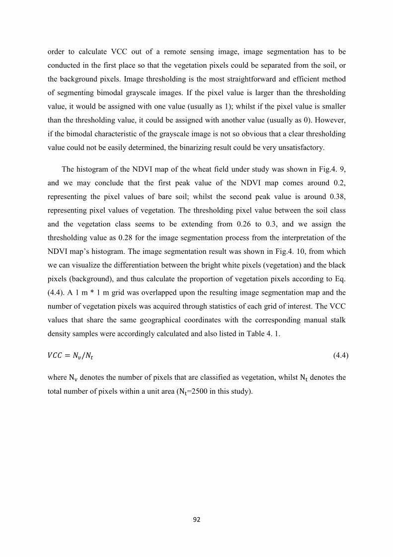
92

order to calculate VCC out of a remote sensing image, image segmentation has to be

conducted in the first place so that the vegetation pixels could be separated from the soil, or

the background pixels. Image thresholding is the most straightforward and efficient method

of segmenting bimodal grayscale images. If the pixel value is larger than the thresholding

value, it would be assigned with one value (usually as 1); whilst if the pixel value is smaller

than the thresholding value, it could be assigned with another value (usually as 0). However,

if the bimodal characteristic of the grayscale image is not so obvious that a clear thresholding

value could not be easily determined, the binarizing result could be very unsatisfactory.

The histogram of the NDVI map of the wheat field under study was shown in Fig.4. 9,

and we may conclude that the first peak value of the NDVI map comes around 0.2,

representing the pixel values of bare soil; whilst the second peak value is around 0.38,

representing pixel values of vegetation. The thresholding pixel value between the soil class

and the vegetation class seems to be extending from 0.26 to 0.3, and we assign the

thresholding value as 0.28 for the image segmentation process from the interpretation of the

NDVI map’s histogram. The image segmentation result was shown in Fig.4. 10, from which

we can visualize the differentiation between the bright white pixels (vegetation) and the black

pixels (background), and thus calculate the proportion of vegetation pixels according to Eq.

(4.4). A 1 m * 1 m grid was overlapped upon the resulting image segmentation map and the

number of vegetation pixels was acquired through statistics of each grid of interest. The VCC

values that share the same geographical coordinates with the corresponding manual stalk

density samples were accordingly calculated and also listed in Table 4. 1.

𝑉𝐶𝐶 = 𝑁𝑣/𝑁𝑡 (4.4)

where Nv denotes the number of pixels that are classified as vegetation, whilst Nt denotes the

total number of pixels within a unit area (Nt=2500 in this study).

93

Fig.4. 9 Histogram of NDVI map

Fig.4. 10 Image segmentation result using thresholding method

In consideration that the spatial resolution of the aerial image reaches up to 2 cm and

there might be plentiful vegetation-background fixed pixels among the pixels of vegetation

and the pixels of soil, an indirect image segmentation method was also utilized to

differentiate vegetation pixels from non-vegetation pixels. Support Vector Machine (SVM)

classification is a supervised machine learning method among many others such as minimum

distance, maximum likelihood, spectral angle mapper, and neural network, which is derived

from statistical learning theory and used for building model of classification, regression, and

94

outlier detection by separating the classes with a decision surface that maximizes the margin

between the classes [87].

Fig.4. 11 Training dataset of SVM classification (in part)

The supervised classification based on SVM technique was conducted by using region of

interest function in ENVI software, which was shown in Fig.4. 11. Training datasets of 200

pixels of vegetation (or highly vegetated pixels, marked with green color in Fig.4. 11) and

200 pixels of background (marked with black color in Fig.4. 11) were manually specified

from the NDVI map, respectively. The training dataset spread all around the wheat field

under study, and the pixels with values larger than 0.4 were assigned as vegetation class

whilst the pixels with values smaller than 0.15 were assigned as non-vegetation class. Thus,

each pixel of the NDVI map was classified either to the class of vegetation or to the class of

non-vegetation according to the SVM classifier, as SVM algorithm separates the classes with

a flexible decision surface from a local neighborhood point of view. The classification result

was shown in Fig.4. 12, in which green pixel represents vegetation whilst the black pixel

represent the background. Confusion matrix was used in ENVI software to validate accuracy

of the classification result by comparing with ground truth of 100 vegetation pixels manually

selected by visual inspection, and the accuracy of the classification result was up to 97.9%.

Subsequently, a 1 m * 1 m grid was also overlapped upon the resulting classification map and

the number of vegetation pixels was acquired through statistics of each grid of interest the

same as how we have dealt with the classification map of thresholding method. The VCC

values that share the same geographical coordinates with the corresponding manual stalk

density samples were accordingly calculated and also listed in Table 4. 1.

95

Fig.4. 12 Classification result using SVM method

4.3 Results and Discussion

4.3.1 Correlation Analysis between Sampled Stalk Density with FGV and VCC

From Table 4. 1 we may understand that VCC values based on the thresholding method

vary from 0.91 to 1.00, which showed severe saturation due to high level of canopy coverage

and is not suitable for building stalk density prediction model in this study. Thus, correlation

analysis between 15 stalk densities sampled by manual counting with the corresponding FGV

and VCC based on SVM method was performed, respectively, by building regression models

in Excel 2010 software (Microsoft Corporation, USA). Fig.4. 13 and Fig.4. 14 showed

different regression models (linear, second-order polynomial, exponential, and power

regression model) between FGV as well as VCC and the sampled stalk densities.

From the figures we may conclude that the regression models between the sampled stalk

densities and FGV values have good accuracy with the coefficient of determination around

0.88; however, the independent variable of FGV has a very limited data range from about 0.4

to about 0.6, indicating that the capacity of FGV of distinguishing different levels of canopy

coverage is rather weak. On the other hand, the regression models between the sampled stalk

densities and VCC values have better accuracy with the coefficient of determination around

0.93. Besides, the independent variable of VCC has a long data range from about 0.3 to about

0.9, indicating that the capacity of VCC of distinguishing different levels of canopy coverage

is stronger when compared to the variable of FGV. And we may conclude that VCC values

96

based on the supervised classification method using the SVM classifier is the most suitable

variable for building regression models to estimate wheat stalk densities from the UAV

remote sensing images.

Fig.4. 13 Regression models between sampled stalk densities with FGV

97

Fig.4. 14 Regression models between sampled stalk densities with VCC

By analyzing the coefficient of determination of four different kinds of regression

models between VCC values and the sampled stalk densities, we may come to the conclusion

that the response variable of stalk density related to the predicator variable of VCC with the

highest coefficient of determination of 0.95 for power regression model, when compared with

that of linear regression model, second-order polynomial regression model, and exponential

regression model as 0.93, 0.94, and 0.91, respectively. And all of these four regression

models have the same RMSE of 24, whilst the mean value of sampled stalk density was

calculated as 593 from the 15 sampled stalk densities. Also, we concluded that around the

VCC value of 0.8, stalk densities showed greater variation and more responsive to changes in

VCC value.

Subsequently, leave-one-out cross-validation (LOOCV) [88] was also conducted by

building 15 linear regression models, second-order polynomial regression models,

exponential regression models, and power regression models, respectively, by using 14 set

variables of sampled stalk densities and VCC as training data, whilst leaving one set of

variables as test data for each regression model. Finally, root-mean-square error of prediction

(RMSEP) [89] for linear regression model, second-order polynomial regression model,

exponential regression model, and power regression model was calculated as 51, 54, 67, and

54, respectively. Taking both coefficient of determination of regression models and RMSEP

of LOOCV models into consideration, power regression model was selected for estimating

and mapping within-field spatial variations of stalk densities by using VCC values based on

vegetation classification result of the UAV ortho-mosaic image.

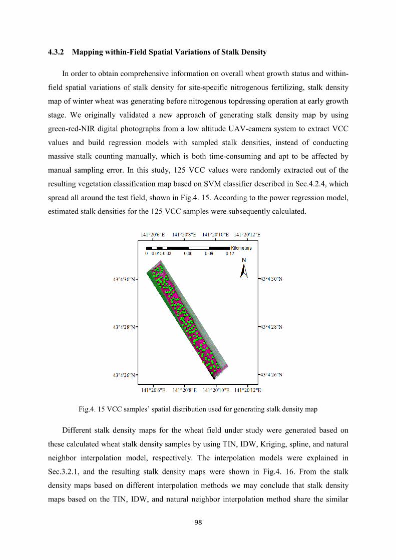
98

4.3.2 Mapping within-Field Spatial Variations of Stalk Density

In order to obtain comprehensive information on overall wheat growth status and within-

field spatial variations of stalk density for site-specific nitrogenous fertilizing, stalk density

map of winter wheat was generating before nitrogenous topdressing operation at early growth

stage. We originally validated a new approach of generating stalk density map by using

green-red-NIR digital photographs from a low altitude UAV-camera system to extract VCC

values and build regression models with sampled stalk densities, instead of conducting

massive stalk counting manually, which is both time-consuming and apt to be affected by

manual sampling error. In this study, 125 VCC values were randomly extracted out of the

resulting vegetation classification map based on SVM classifier described in Sec.4.2.4, which

spread all around the test field, shown in Fig.4. 15. According to the power regression model,

estimated stalk densities for the 125 VCC samples were subsequently calculated.

Fig.4. 15 VCC samples’ spatial distribution used for generating stalk density map

Different stalk density maps for the wheat field under study were generated based on

these calculated wheat stalk density samples by using TIN, IDW, Kriging, spline, and natural

neighbor interpolation model, respectively. The interpolation models were explained in

Sec.3.2.1, and the resulting stalk density maps were shown in Fig.4. 16. From the stalk

density maps based on different interpolation methods we may conclude that stalk density

maps based on the TIN, IDW, and natural neighbor interpolation method share the similar

99

general trend with the stalk density varying from about 40 to about 900 stalks per square

meter, whilst stalk density maps based on the Kriging and spline interpolation model

indicated unsuitable and inaccurate estimation of the within-field varying wheat stalk

densities.

Fig.4. 16 Resulting stalk density maps based on TIN, IDW, Kriging (upper images from left to right),

spline, and natural neighbor (bottom images from left to right) interpolation method

Table 4.4 Sampled stalk densities and estimated stalk densities based on different interpolation

models

Sample

ID Latitude Longitude

Sampled

Stalk Density

Estimated Stalk Densities Based on

Different Interpolation Models

TIN IDW Kriging Spline Natural

Neighbor

1 43.07396

5

141.336014 690 693 711 416 686 693

2 43.07404

4

141.336031 400 377 369 463 364 370

3 43.07408

3

141.335921 660 702 696 524 679 660

4 43.07413

0

141.335869 620 605 616 567 618 605

5 43.07417

4

141.335898 490 439 451 539 439 454

100

6 43.07428

8

141.335735 850 735 780 655 777 754

7 43.07438

0

141.335647 800 573 729 652 721 652

8 43.07439

3

141.335719 560 504 486 652 476 496

9 43.07450

0

141.335636 290 318 303 539 282 295

10 43.07454

5

141.335496 710 634 636 538 637 617

11 43.07475

7

141.335321 570 592 604 584 592 595

12 43.07475

8

141.335407 680 722 770 584 768 756

13 43.07484

4

141.335250 660 674 705 575 707 697

14 43.07497

6

141.335123 720 760 757 577 775 765

15 43.07509

6

141.335155 200 233 222 280 241 241

Fig.4. 17 Variation of estimated stalk densities based on different interpolation methods

Subsequently, estimated stalk density values were extracted from the resulting stalk

density map based on different interpolation models according to the geographical

coordinates of the manual samples. The accuracies were also confirmed by calculating

RMSEs between the 15 manually sampled stalk density values and the corresponding

estimated stalk density values extracted from each stalk density map based on TIN, IDW, and

natural neighbor interpolation model, as 75, 51, and 62, respectively. For reference, the

average value of the manually sampled stalk density was calculated as 593 stalks per square

meter. By observing the variations of estimated stalk density based on different interpolation

methods from Fig.4. 17, the stalk density map based on IDW interpolation model was

selected to demonstrate the within-field spatial variation of wheat stalk density. From the

IDW interpolation method based stalk density map we may conclude that the field under

101

study has a spatially varying stalk density ranging from 40 to 906 stalks per square meter. We

can also understand that the headland of both sides has a relatively lower stalk density, and

several low-stalk-density areas could also be spotted distributing all over the wheat field

shown in red color.

𝑅𝑀𝑆𝐸𝑠𝑡𝑎𝑙𝑘𝑇𝐼𝑁 = √∑ (𝑆𝑚𝑎𝑛𝑢𝑎𝑙𝑖−𝑆𝑇𝐼𝑁𝑖)15𝑖=1

2

15 (4.5)

𝑅𝑀𝑆𝐸𝑠𝑡𝑎𝑙𝑘𝐼𝐷𝑊 = √∑ (𝑆𝑚𝑎𝑛𝑢𝑎𝑙𝑖−𝑆𝐼𝐷𝑊𝑖)15𝑖=1

2

15 (4.6)

𝑅𝑀𝑆𝐸𝑠𝑡𝑎𝑙𝑘𝑁𝑎𝑡 = √∑ (𝑆𝑚𝑎𝑛𝑢𝑎𝑙𝑖−𝑆𝑁𝑎𝑡𝑖)15𝑖=1

2

15 (4.7)

where 𝑅𝑀𝑆𝐸𝑠𝑡𝑎𝑙𝑘𝑇𝐼𝑁 , 𝑅𝑀𝑆𝐸𝑠𝑡𝑎𝑙𝑘𝐼𝐷𝑊 , and 𝑅𝑀𝑆𝐸𝑠𝑡𝑎𝑙𝑘𝑁𝑎𝑡 is the root mean square error

between the reference stalk density values by manual sampling and stalk density values

extracted from the stalk density maps based on TIN interpolation model, IDW interpolation

model, and natural neighbor interpolation model, respectively; whilst 𝑆𝑚𝑎𝑛𝑢𝑎𝑙, 𝑆𝑇𝐼𝑁, 𝑆𝐼𝐷𝑊,

and 𝑆𝑁𝑎𝑡 the reference stalk density values by manual sampling and stalk density values

extracted from the stalk density maps based on TIN interpolation model, IDW interpolation

model, and natural neighbor interpolation model, respectively.

From the histogram of the stalk density map based on IDW interpolation method we

obtained the information that the average value and standard deviation of the stalk density of

the field was 554 and 136 stalks per square meter, respectively. About 12% acreages of the

studied field have the stalk density ranging from 800 to 1000 stalks per square meter, which

need low dose of nitrogenous topdressing such as 30 kg/10a ammonium sulfate; whilst about

22% acreages of the studied field have the stalk density ranging from 600 to 800 stalks per

square meter, which need moderate dose of nitrogenous topdressing such as 40 kg/10a

ammonium sulfate; and about 66% acreages of the field have the stalk density lower than 600

stalks per square meter, which desperately need high dose of nitrogenous topdressing such as

50 kg/10a or more ammonium sulfate for generating enough stalks before the end of tillering

stage. There are no part of this field has the stalk density beyond 1500 stalks per square meter,

indicating that there are no over-flourished canopies that would lead to the occurrence of

lodging in later growth stage.

102

Fig.4. 18 Histogram of estimated stalk density map based on IDW interpolation method

4.4 Experimental Validation of the Stalk Density Estimation Model

Table 4. 5 Sampled stalk densities and the corresponding VCC values of validating experiment

Sample

ID Latitude Longitude

Sampled

Stalk Density

VCC

(SVM)

Estimated

Stalk Density

1 43.07486

262

141.334477

83

570 0.60 602

2 43.07482

364

141.334689

88

140 0.12 126

3 43.07468

099

141.334633

83

790 0.82 814

4 43.07459

920

141.334886

42

830 0.84 833

5 43.07449

290

141.334839

41

720 0.66 660

6 43.07444

997

141.334987

56

600 0.59 592

7 43.07435

416

141.334923

17

360 0.39 396

8 43.07437

925

141.335089

13

700 0.64 640

9 43.07421

956

141.335068

61

690 0.66 660

10 43.07426

166

141.335208

38

330 0.34 347

11 43.07409

751

141.335233

77

270 0.31 317

12 43.07414

395

141.335364

96

610 0.63 631

13 43.07393

938

141.335357

95

560 0.63 631

14 43.07391

121

141.335506

18

590 0.51 514

15 43.07381

541

141.335441

54

770 0.72 718

The validating experiment on the accuracy and repeatability of the stalk density

estimation model was conducted for anther wheat field of the Hokkaido University on 20

May 2017. The test field was described in Sec.2.3.1 and shown in Fig.2. 9, where the

topographic mapping experiment was conducted. The same wheat variety and seeding rate

was applied with another wheat field of previous year that was described in Sec.4.2.1. 15

stalk densities were also manually sampled as ground truth and the geographical coordinates

103

of each sample was measured by using the same RTK-GPS module described in Sec.4.2.2.

The spatial distribution of these stalk densities was shown in Fig.4. 19 as red dots, and the

geographical coordinates as well as the stalk density values were listed in Table 4. 5.

Similarly, each 200 vegetation pixels and background pixels were selected from the resulting

NDVI map with the ground resolution of about 2 cm as training data through visual

inspection, respectively; and by means of the supervised classification method of SVM

classifier, the VCC map of the wheat field was generated for the validating experiment. The

resulting VCC map was shown in Fig.4. 19, in which the green pixels represent vegetation

class and the white pixels represent the background class. From the VCC map we may

understand that the areas circled in red color have no sign of vegetation, as the wheat plants

over there were drowned in the snowmelt water during the early April due to the relatively

low ground elevation, also discussed in Sec.3.3.2.

Fig.4. 19 Vegetation classification result of wheat field for validating experiment

VCC values of the areas that share the same geographical coordinates with each

corresponding manually sampled stalk density were subsequently obtained and also listed in

Table 4. 5. Different regression models between the manually sampled stalk density values

with the corresponding VCC values were built, as shown in Fig.4. 20, from which we can

come to the conclusion that power regression model with the coefficient of determination of

104

0.97 is still the most accurate one for estimating wheat stalk density by using the calculated

VCC values.

Fig.4. 20 Regression models between sampled stalk densities with VCC for validating experiment

Finally, 125 VCC values were extracted from Fig.4. 19 that randomly distributed all

around the field under study; and the corresponding stalk densities were estimated from the

power regression model; then, the stalk density map was generated by using these 125

estimated stalk density samples based on the IDW interpolation method, shown in Fig.4. 21.

From Fig.4. 21 we can see that the south part of the field has a relatively lower stalk density,

and in consideration of the topographic map shown in Fig.3. 16 we may conclude that

plentiful and stagnant snowmelt water is harmful to the survival and development of wheat

plant, which might led to the worst situation of total crop failure over the areas of relatively

low ground elevation. The RMSE between the manually sampled stalk density values and

each corresponding stalk density values that were extracted out of the resulting stalk density

map based on the IDW interpolation model were calculated as 43 stalks per square meter,

105

which showed acceptable accuracy and practical feasibility in comparison with the average

value of the manually sampled wheat stalk density of 569 stalks per square meter.

𝑅𝑀𝑆𝐸𝑠𝑡𝑎𝑙𝑘𝑉𝑎𝑙 = √∑ (𝑆𝑚𝑎𝑛𝑢𝑎𝑙𝑉𝑎𝑙𝑖−𝑆𝑉𝑎𝑙𝑖)15𝑖=1

2

15 (4.8)

where 𝑅𝑀𝑆𝐸𝑠𝑡𝑎𝑙𝑘𝑉𝑎𝑙 is the root mean square error between the stalk density values by manual

sampling and the stalk density values that were extracted out of the resulting stalk density

map based on the IDW interpolation model; whilst 𝑆𝑚𝑎𝑛𝑢𝑎𝑙𝑉𝑎𝑙, and 𝑆𝑉𝑎𝑙 is the reference stalk

density values by manual sampling and the stalk density values that were extracted out of the

resulting stalk density map based on the IDW interpolation model, respectively.

Fig.4. 21 Estimated stalk density map for validating experiment

From the histogram of the estimated stalk density map based on IDW interpolation

method we obtained the information that the minimum and maximum stalk density value was

0 and 939 stalks per square meter, respectively, with the average value of 508 stalks per

square meter. We may also understand that about 15% acreages of the studied field have the

stalk density ranging from 800 to 1000 stalks per square meter, which need low dose of

nitrogenous topdressing such as 30 kg/10a ammonium sulfate; whilst about 21% acreages of

the studied field have the stalk density ranging from 600 to 800 stalks per square meter,

which need moderate dose of nitrogenous topdressing such as 40 kg/10a ammonium sulfate;

106

and about 64% acreages of the field have the stalk density lower than 600 stalks per square

meter, which desperately need high dose of nitrogenous topdressing such as 50 kg/10a or

more ammonium sulfate for generating enough stalks before the end of tillering stage. There

are no part of this field has the stalk density beyond 1500 stalks per square meter, indicating

that there are no over-flourished canopies that would lead to the occurrence of lodging in

later growth stage.

Fig.4. 22 Histogram of estimated stalk density map for validating experiment.

4.5 Conclusion

The novel approach of obtaining spatially-varied stalk density information of winter

wheat at early growth stage by using UAV images and ground samples, which was described

in this paper in detail, provides an accurate, time-and-cost efficient alternative of generating

site-specific fertilizing prescription for precision agriculture. The aerial images were stitched

as an ortho-mosaic image and further post-processed by geo-referencing. Subsequently map

of normalized difference vegetation index (NDVI) was generated; then NDVI map was

binarized as vegetation and background, and fractional green vegetation (FGV) as well as

vertical canopy coverage (VCC) was calculated out of the binarization result. Finally

regression models were built between the manually sampled stalk density values and the

corresponding FGV and VCC values.

From the comparison of the extracted values of FGV, thresholding method based VCC,

and support vector machine (SVM) classifier based VCC, we came to a conclusion that the

Stalk density (stalks per square meter)

Fre

qu

ency

107

conventional thresholding method is the simplest image segmentation tool but not suitable for

this study of estimating wheat stalk density from UAV remote sensing images, as the

important thresholding value is usually not clear for segmenting the vegetation pixels from

the non-vegetation pixels in aerial remote sensing images. The directly generated FGV values

by determining NDVI value of the soil and the maximum NDVI value showed good

correlation with the corresponding manually sampled stalk density values. Nevertheless, the

FGV values concentrated to a very short range, indicating that the capability of distinguishing

different levels of canopy coverage is limited. On the other hand, supervised classification

based on SVM classifier needs massive human intervention by selecting training dataset from

the NDVI map; however, VCC values extracted from the resulting classification map based

on SVM classifier had a considerably wide range and the correlation with the corresponding

manually sampled stalk density values is also very strong, due to the flexible decision surface

of the SVM classifier that maximizes the margin between the vegetation class and the

background class.

Based on the extracted FGV values as well as the SVM classifier based VCC values and

the corresponding samples of stalk density acquired through manual counting, different kinds

of regression models such as linear, second-order polynomial, exponential, and power

regression models were built, respectively. And we may conclude that the regression models

based on FGV values have good accuracy with the coefficient of determination around 0.89,

and the regression models based on VCC values have better accuracy with the coefficient of

determination around 0.94. Furthermore, we selected the power regression model between

manually sampled stalk density values and the corresponding SVM classifier based VCC

values for generating stalk density map for the wheat field under study, which has a high

coefficient of determination of 0.95 and root-mean-square error of 24, in consideration that

the average value of the manually sampled stalk density values was calculated as 593 stalks

per square meter. The validating experiment on the other wheat field with the same seeding

rate and similar field management treatment also confirmed that the power regression model

is the most accurate and suitable model between the manually sampled stalk density values

and the SVM classifier based VCC values. According to the power regression model between

stalk density values and SVM classifier based VCC values, 125 stalk density values were

calculated by extracting the corresponding VCC values from the resulting vegetation

classification map based on SVM classification method. Subsequently, stalk density maps

were generated out of the calculated stalk density values by using triangular irregular network,

108

inverse distance weight (IDW), spline, Kriging, and natural neighbor interpolation method,

respectively. As the result, IDW interpolation method based stalk density map was selected to

demonstrated stalk densities’ within-field spatial variations and different rate of nitrogenous

topdressing could be suggested accordingly.

In thus, we would like to conclude that the UAV-camera system used in this study could

be used to obtain quantitative information for variable-rate topdressing in terms of site-

specific or precision agriculture in an accurate and efficient manner. Also, the UAV-camera

system presented here can be used for vegetation monitoring in various applications of

determining plant cover or above-ground biomass estimation, and fulfil the need for remote

sensing of high ground resolution imagery at low cost.

109

Chapter 5 Multi-temporal Monitoring of Wheat Growth Status and

Mapping within-Field Variations of Wheat Yield

5.1 Introduction

In Chapter 4 we monitored wheat growth status during the early growth stage (tillering

stage), and concluded that the low altitude UAV-camera system could be practically used as a

powerful tool for quantitative analysis between wheat stalk density and remote sensing

images. However, we cannot assert that the monitoring of wheat growth status is no longer

needed after the tillering stage, as the field condition during the reproductive growth stages

(booting stage, heading stage, flowering stage, dough development stage, and ripening stage)

plays an even more important role in the yield formation, grain moisture content estimation,

as well as the protein concentration. In order to optimize wheat yield and grain quality,

especially in terms of protein content that varies significantly depending on different

agricultural practices, wheat growers are expected to have a detailed understanding of wheat

growth status during each specific development stage in wheat cultivation [90]. It implies that

real-time monitoring of actual wheat growth status throughout the wheat growing season is of

vital importance in helping wheat growers with management decision making. Meanwhile, it

was frequently reported that reproductive growth of wheat after the flowering stage is closely

related to grain yield, and many studies in recent years on wheat growth have indicated that

accumulative vegetation index values of multi-temporal satellite remote sensing images after

flowering stage have good relationship with crop yield [91]-[93]. Besides, Okuno studied on

the wheat harvest support system by using satellite images during late-season of wheat

growth stages in order to optimize harvest timing at regional scale, and generated a

harvesting sequence map covering about 4000 ha [94]. And Han-ya and et al. investigated the

correlation between the moisture content of wheat ear and the satellite and helicopter imagery,

and accordingly reduced estimation error of moisture content [95].

Lodging, which usually occurs during wheat’s ripening growth stage when ears fall over

and rot on the ground, is another big concern especially for wheat growers in Hokkaido,

Japan, as the storms and rainfalls usually coincide with the ripening process of winter wheat

in the middle of July. Heavy nitrogenous fertilization makes wheat stalk grow taller and

become more susceptible to this problem, and cautions are increasingly paid to the

110

application of nitrogenous fertilizers giving consideration to both desired wheat stalk density

and the avoidance of heavy lodging situation. Adverse impacts of the occurrence of lodging

in wheat field are tremendous. It not only affects the grain quality due to rot but also hinders

the harvesting operation of combine harvester in the following aspects, as jam fault of

combine harvester by the over-high humidity of the lodged wheat stalks is a typical failure. In

the first place, the cutting process could be interrupted when the gap between moving blade

and fixed blade is suffused by wheat stalks with high wetness. More likely, the threshing

drum is apt to be entangled with the succulent wheat stalks; and as more and more wheat

stalks stagnate upon the drum, it eventually gets stalled or even leads to the failure of the

combine harvester’s transmission system. Lastly, even if the wet wheat stalks successfully

went through the cutting and threshing mechanisms of the combine harvester, it would

inevitably “smuggle” plentiful grains by mixing and sheltering them from the sieves, which

gives rise to extra yield loss [96], illustrated in Fig.5. 1. Since the “harvesting window” is

usually very limited and we cannot afford wasting any moment in fixing or repairing the

broken machine, the lodging situation of the wheat field is in desperate need before the

harvesting operation so that drivers or the autonomous combine harvester could adjust

working velocity accordingly.

Fig.5. 1 Working principle of a combine harvester (Missotten, 1998)

As we have discussed in Sec.1.1.2 that satellite images can be regularly obtained at large

scale, the ground resolution is yet inadequate for quantitative analysis that aims at

demonstrating within-field variations. Besides, the minimum purchasing area of the satellite

111

images often starts from 2000 ha or so and it still increases if the ground resolution of the

image gets more sparse. For example, the minimum purchasing area of WorldView satellite

images with the ground resolution of about 50 cm is set as 2500 ha, whilst the minimum

purchasing area of RapidEye satellite images with the ground resolution of about 5 m is set as

50 000 ha [97], [98]. For comparison, the average value of farmland area under cultivation

per farmer was surveyed as 2.4 ha in the year of 2016 in Japan [99]. Using satellite images

for multi-temporal monitoring of field condition and thus putting forward corresponding field

management decisions seems neither particularly economical nor practical for both individual

farmers and small farming-related organizations, not even to speak of the unavailability of a

specific area due to cloud shadows, and etc.

In recent years, civilian applications of small UAVs have widespread from entertainment

industry to professional photogrammetry, hazard survey, crop protection, and remote sensing,

etc., as UAV image has increasing spatial resolution, may be acquired more cost-effectively

and with excellent maneuverability as well as greater safety when compared with manned

aircrafts [100]. Besides, agricultural application of UAV remote sensing by using commercial

color cameras decreases high cost of remote sensing sharply and provides instantly

researchers and farmers with actual and intuitive visualization of crop growth status, since

color images accentuate particular vegetation greenness and have been suggested to be less

sensitive to variations of illumination conditions [101]-[103]. Furthermore, several vegetation

indices based on color images were proposed such as visible-band difference vegetation

index (VDVI) [102], among other color vegetation indices of normalized green-red difference

index (NGRDI) [104], normalized green-blue difference index (NGBDI) [105], and green-red

ratio index (GRRI) [104], and excessive greenness (ExG) [105]. Woebbecke et al. tested

several color indices derived by using chromatic coordinates and modified hue to distinguish

vegetation from background such as bare soil and crop residues [105], among which ExG

provides a near-binary intensity image outlining a plant region of interest has been widely

cited. Wang and et al. [102] distinguished vegetative areas from non-vegetative areas by

analyzing color images acquired from a UAV and found VDVI has the most precise

capability of extracting vegetation areas in comparison with other vegetation indices of

NGRDI, NGBDI, GRRI, and ExG. Rasmussen and et al. [76] investigated four different

vegetation indices acquired from a color camera and a color-infrared camera by using both a

fixed-wing and a rotary-wing UAV, and concluded that vegetation indices based on UAV’s

RGB image have the same ability to quantify crop responses with ground-based recordings.

112

Torres-Sánchez et al. mapped multi-temporal vegetation fraction in early-season wheat fields

by using a UAV equipped with a commercial color camera and studied the influence of flight

altitude and growing days after sowing on the classification accuracy, which showed that

visible spectral vegetation indices derived from low-altitude UAV-camera system could be

used as a suitable tool to discriminate vegetation in wheat fields in the early season [104]. Cui

et al. evaluated the reliability of using color digital images to estimate above ground biomass

at canopy level of winter wheat by taking pictures from one meter above the top of the wheat

canopy [106]. In short, most past agricultural studies on color images focused on individual

level of crop or weed, and the point-source samplings of which are usually inevitably both

time-consuming and have to be conducted under poor working condition.

Therefore, in this study we monitored the time-varying canopy status of wheat through

both the multispectral satellite images and also the UAV’s RGB images. Subsequently, we

investigated correlations between vegetation indices of UAV’s RGB images and

multispectral satellite images for future study of temporal complementation of these two

different remote sensing systems. Correlation analysis between vegetation indices with

sampled grain yield was also conducted, and the yield map that demonstrated the within-field

spatial variations was generated accordingly.

5.2 Methodology

Four satellite images as well as eight UAV ortho-mosaic images during the late-season

of wheat growth stages were utilized extending from the early June to the late July of 2015

for multi-temporally monitoring wheat growth status and mapping within-field variations of

wheat yield. Firstly, UAV ortho-mosaic images were generated and geo-referenced to be

aligned with satellite images; then different vegetation indices were extracted from each

remote sensing images; subsequently, wheat growth status was monitored from both the

multi-temporal remote sensing images and also the vegetation index maps; finally, within-

field variations of yield was mapped according to the result of correlation analysis among the

vegetation indices and ground samples of wheat yield.

5.2.1 Field Site and Remote Sensing Images

Experiments were established on two neighboring fields, which were planted with two

different winter wheat varieties of Kitahonami and Yumechikara around 25 September 2014

and harvested on 27 July 2015. Fig.5. 2 showed the location of the investigated farmland in

113

Memuro, Hokkaido, Japan (around 42.902041°N–42.899607°N and 142.977953°E–

142.981734°E). From weather data of 1981-2015 [106], regional annual precipitation,

average annual temperature, and average accumulative annual duration of sunshine of this

area is reported as 953.3 mm, 6.2°C, and 1939.6 h, respectively; whilst in 2015 annual

precipitation, average annual temperature, and accumulative annual duration of sunshine of

this area is reported as 828.5 mm, 7.0°C, and 2115.0 h, respectively. The lower left field

No.1 (marked in black rectangle shown in Fig.5. 2) and upper right field No.2 (marked in red

rectangle shown in Fig.5. 2) was planted with wheat variety of Kitahonami and Yumechikara,

respectively. Each of these two fields occupies about 3.2 ha and 2 ha, of which the variety of

Kitahonami is the most widely planted winter wheat variety in Japan and is reported to have

taken up about 90% acreages of winter wheat in Hokkaido alone[108].

Fig.5. 2 Two neighboring wheat fields were studied planted with different winter wheat varieties

Fig.5. 3 Color change of wheat canopy shown by using satellite images in true color mode (Images

taken on June 1, 7, 15, and July 17, 2015 were demonstrated in sequence from left to right)

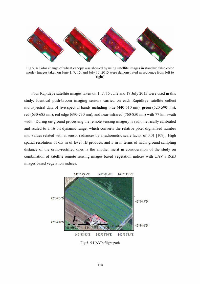
114

Fig.5. 4 Color change of wheat canopy was showed by using satellite images in standard false color

mode (Images taken on June 1, 7, 15, and July 17, 2015 were demonstrated in sequence from left to

right)

Four Rapideye satellite images taken on 1, 7, 15 June and 17 July 2015 were used in this

study. Identical push-broom imaging sensors carried on each RapidEye satellite collect

multispectral data of five spectral bands including blue (440-510 nm), green (520-590 nm),

red (630-685 nm), red edge (690-730 nm), and near-infrared (760-850 nm) with 77 km swath

width. During on-ground processing the remote sensing imagery is radiometrically calibrated

and scaled to a 16 bit dynamic range, which converts the relative pixel digitalized number

into values related with at sensor radiances by a radiometric scale factor of 0.01 [109]. High

spatial resolution of 6.5 m of level 1B products and 5 m in terms of nadir ground sampling

distance of the ortho-rectified ones is the another merit in consideration of the study on

combination of satellite remote sensing images based vegetation indices with UAV’s RGB

images based vegetation indices.

Fig.5. 5 UAV’s flight path

115

Fig.5. 6 UAV’s RGB images from heading stage to harvesting (the upper four images from left to

right were taken on June 2, 10, 19 and 25, and the lower four images from left to right were taken on

July 2, 10, 16 and 24, 2015)

Since satellite remote sensing images’ temporal frequencies and spatial resolution are not

adequate to monitor rapidly changing wheat growth conditions, eight RGB images acquired

from UAV were also taken from early June to the end of July 2015 covering two wheat fields

at the interval of about one week. Autonomous flights were conducted eight times from

winter wheat’s heading stage to ripening stage, on 2, 10, 19, and 25 June, 2015, and 2, 10, 16,

and 24 July 2015 (at about 11:00 local time), using the flight paths that were designed

beforehand in the GCS software, shown in Fig.5. 5 as blue lines. A SONY ILCE-6000

commercial digital camera with the sensor size of 23.5 mm * 15.6 mm and the focal length of

16 mm was used to take pictures in continuous mode every two seconds (f/8, 1/500 sec, ISO

100). During each flight the camera was fixed on a two-axis gimbal, pointing vertically

downwards and took about 120 photos covering two adjacent fields in order to get enough

GCPs for geo-referencing. Every 120 individual photographs were stitched together as an

Ortho-mosaic image by using Agisoft Photoscan software, which was shown in Fig.5. 6.

Each of the Ortho-mosaic images has about 3600 * 2450 pixels in size, and the ground

resolution reached up to about 12.5 cm after ortho-mosaicking. Geo-referencing of UAV

ortho-mosaic images were accomplished using ArcMap software by using eight GCPs, which

consist of headline corners, telegraph poles around the test field. First order polynomial

transformation creates two least-square-fit equations by comparing the image space

coordinates of the GCPs with the geographic coordinates (latitude and longitude) and

translates image coordinates of each pixel into geographic coordinates. These GCPs’ geo-

116

spatial coordinates were measured by using Trimble SPS855 GNSS modular receiver in

RTK-GPS mode. And the result of UAV Ortho-mosaic image’s geo-referencing was shown

in Fig.5. 7 as geo-spatially overlaid upon a satellite image.

Fig.5. 7 Geo-referenced UAV’s Ortho-mosaic image overlaid upon satellite image

5.2.2 Radiometric Normalization of Multi-temporal Remote Sensing Images

Due to variated atmospheric conditions, different illumination intensity, viewing angles,

and etc., radiometric accuracy and consistency are difficult to maintain among multi-temporal

remote sensing images. Different from absolute radiometric correction, which is usually

based on radiative transfer models such as 6S [110], MODTRAN [111], and etc., relative

radiometric correction or radiometric normalization was performed to adjust multi-temporal

images to a set of reference data and compensate for the above effects. The reference data

were generated by calculating the average values of each pseudo-invariant features’ (PIF)

pixel values, band by band, which refer to the ground objects of which the reflectance values

are nearly constant over time during a certain period [112]. According to these PIFs’ pixel

values of each band and corresponding reference data, the radiometric normalization models

of different dates’ satellite images as well as UAV ortho-mosaic images, band by band, were

obtained by building linear regression equations.

As to the satellite images, 38 crossroads and 2 flat grounds nearby construction sites,

covering considerable large area around the experimental field, were selected as PIFs by

visual inspection, marked as dark dots shown in Fig.5. 8. Forty PIFs’ pixel values and the

corresponding average values are listed in Table 5. 1, taking blue band as an example. 7

117

places along road as well as 5 places on roofs were chosen as PIFs in each UAV ortho-

mosaic images, and around each PIF’s location the average value of 6 pixels distributed

within 1-meter-square were calculated so that the influence of abnormal values caused by

foreign matters etc. could be decreased to the minimum. The spatial distribution of UAV

Ortho-mosaic images’ PIFs was also shown in Fig.5. 8.

Table 5. 1 PIFs’ pixel values of satellite images (taking blue band as an example)

PIF ID 17 July 15 June 7 June 1 June Average

1 8046 8827 8846 8775 8624

2 6161 7684 7229 7374 7112

3 6704 8107 7532 7477 7455

4 6478 7817 7035 7190 7130

5 7761 8605 7939 8083 8097

6 6726 7864 6685 7218 7123

7 5997 8042 6759 7606 7101

8 6613 8065 7328 7615 7405

9 6213 7927 7232 7191 7141

10 7288 8281 7694 8002 7816

11 6705 7998 7954 7636 7573

12 6624 8565 7128 6960 7319

13 6070 7720 6872 6914 6894

14 6766 8013 7288 7436 7376

15 6645 7937 7187 7497 7317

16 6466 8268 7561 7208 7376

17 7287 8070 7062 7773 7548

18 5889 7405 6327 6752 6593

19 6603 7869 7603 7946 7505

20 6950 7860 6739 7153 7176

21 6657 8023 7502 7040 7306

22 6991 8268 7957 7773 7747

23 6936 7948 7714 8023 7655

24 5561 7680 6668 7136 6761

25 6963 8212 7308 6926 7352

26 6326 7912 7509 7771 7380

27 5961 8014 6508 6863 6837

28 11228 9701 10003 11163 10524

29 6798 8116 7659 7940 7628

30 6720 8107 7937 7865 7657

31 6033 7551 6428 7059 6768

32 6214 7803 6605 7227 6962

33 6261 7855 6797 7574 7122

34 6997 8122 7267 7349 7434

35 12584 11324 12723 15994 13156

36 7938 8688 8278 8186 8273

37 6888 7979 7200 7651 7430

38 5933 7948 7271 7381 7133

118

39 6224 7996 6380 6791 6848

40 5801 7823 6446 7091 6790

Fig.5. 8 Spatial distribution PIFs in satellite image (left) and UAV Ortho-mosaic image (right)

Table 5. 2 Linear regression normalization models of satellites images

Image date Band Slope Intercept R-squared

1 June Blue 0.72 1977.00 0.96

Green 0.76 1419.83 0.98

Red 0.81 830.67 0.97

RE 0.80 917.50 0.98

NIR 0.90 710.89 0.87

7 June Blue 0.98 228.58 0.95

Green 0.94 443.09 0.99

Red 1.04 -306.32 0.96

RE 1.00 -104.54 0.96

NIR 0.83 1444.00 0.91

15 June Blue 1.68 -6117.00 0.94

Green 1.52 -3627.00 0.93

Red 1.25 -993.83 0.89

RE 1.24 -877.75 0.90

NIR 0.98 -369.56 0.84

17 July Blue 0.84 1817.00 0.95

Green 0.90 962.98 0.94

Red 0.83 1029.00 0.96

RE 0.89 620.13 0.97

NIR 0.80 169.00 0.86

119

Table 5.3 Linear regression normalization models of UAV images

Image date Band Slope Intercept R-squared

2 June Blue 1.01 6.55 0.83

Green 0.77 45.38 0.96

Red 0.74 52.52 0.94

10 June Blue 0.86 15.43 0.73

Green 0.87 7.96 0.91

Red 0.85 11.55 0.91

19 June Blue 0.77 42.65 0.91

Green 1.09 -15.09 0.94

Red 1.10 -17.33 0.93

25 June Blue 0.99 4.14 0.97

Green 0.95 9.63 0.99

Red 0.92 12.56 0.99

2 July Blue 0.82 28.49 0.94

Green 1.03 -13.48 0.98

Red 1.03 -12.15 0.98

10 July Blue 0.88 22.77 0.81

Green 1.01 -2.42 0.94

Red 1.06 -10.30 0.93

16 July Blue 0.79 47.09 0.97

Green 1.16 -15.27 0.98

Red 1.16 -16.84 0.97

24 July Blue 0.94 12.01 0.80

Green 0.89 17.61 0.97

Red 0.90 16.28 0.97

According to these PIFs’ pixel values, radiometric normalization models of different

dates’ satellite images as well as UAV ortho-mosaic images, band by band, were built and

shown in Table 5. 2 and Table 5.3, respectively. From the results of R-squared values we can

see that the deviation of the satellite image on 15 June from the reference data is most

significant, which means the atmospheric effects such as weather condition comparatively

differ from other days. When considered from the viewpoint of the performances of each

band, NIR band of the satellite images expressed worst correlation, and the other bands

seemed to be correspondingly correlated better among these images, due to different spectral

responsive characteristics. As to UAV ortho-mosaic images, conclusion could be drawn that

the variation of blue band is most significant, whilst green band and red band expressed

consistently higher relevance and less variation, indicating that blue band is more susceptible

to influences of different photographing environment. And we can also conclude that the

image of 10 June was taken under the most deviated photographing condition when

120

compared to other UAV ortho-mosaic images. And based on these linear regression models,

each band of all images was radiometrically normalized to the reference data and the effects

caused by the deviation of atmosphere condition could be compensated, so that we can ignore

the disturbance of atmosphere and extract the real changes of crops in multi-temporal

analysis.

5.2.3 Vegetation Indices of Remote Sensing Images

Fig.5. 9 Typical spectral signature of different features (Saba Daneshgar)

NDVI is the most well-known and widely used vegetation index to detect live plant

canopies due to the high spectral reflectance of plants in the spectrum of NIR region. In

recent years several vegetation indices that are different from the NDVI associated with NIR

band were proposed based on high-resolution color remote sensing images, in order to

identify vegetative features from background such as VDVI, NGRDI, NGBDI, GRRI, and

ExG mentioned above in Sec.5.1, according to the typical spectral signature of different

features shown in Fig.5. 9.

𝑁𝐷𝑉𝐼 = (𝑁𝐼𝑅 − 𝑅𝑠𝑎𝑡𝑒)/(𝑁𝐼𝑅 + 𝑅𝑠𝑎𝑡𝑒) (5.1)

𝑉𝐷𝑉𝐼𝑠𝑎𝑡𝑒 = (2𝐺𝑠𝑎𝑡𝑒 − 𝑅𝑠𝑎𝑡𝑒 − 𝐵𝑠𝑎𝑡𝑒)/(2𝐺𝑠𝑎𝑡𝑒 + 𝑅𝑠𝑎𝑡𝑒 + 𝐵𝑠𝑎𝑡𝑒) (5.2)

𝑉𝐷𝑉𝐼 = (2𝐺𝑈𝐴𝑉 − 𝑅𝑈𝐴𝑉 − 𝐵𝑈𝐴𝑉)/(2𝐺𝑈𝐴𝑉 + 𝑅𝑈𝐴𝑉 + 𝐵𝑈𝐴𝑉) (5.3)

𝑁𝐺𝑅𝐷𝐼 = (𝐺𝑈𝐴𝑉 − 𝑅𝑈𝐴𝑉)/(𝐺𝑈𝐴𝑉 + 𝑅𝑈𝐴𝑉) (5.4)

121

𝑁𝐺𝐵𝐷𝐼 = (𝐺𝑈𝐴𝑉 − 𝐵𝑈𝐴𝑉)/(𝐺𝑈𝐴𝑉 + 𝐵𝑈𝐴𝑉) (5.5)

𝐺𝑅𝑅𝐼 = 𝐺𝑈𝐴𝑉/𝑅𝑈𝐴𝑉 (5.6)

𝐸𝑥𝐺 = 2𝐺𝑈𝐴𝑉 − 𝑅𝑈𝐴𝑉 − 𝐵𝑈𝐴𝑉 (5.7)

where 𝑁𝐼𝑅, 𝑅𝑠𝑎𝑡𝑒, 𝐺𝑠𝑎𝑡𝑒 and 𝐵𝑠𝑎𝑡𝑒 is the radiometrically normalized pixel value of NIR band,

red band, green band and blue band of satellite images, respectively; whilst 𝐺𝑈𝐴𝑉, 𝑅𝑈𝐴𝑉, and

𝐵𝑈𝐴𝑉 is the radiometrically normalized pixel values of green band, red band and blue band of

UAV’s ortho-mosaic images, respectively.

Fig.5. 10 Spatial distribution of vegetation indices

In this study, forty vegetation indices’ samples (each twenty samples for field

Kitahonami and Yumechikara, respectively) of NDVI as well as VDVIsate out of each

satellite images were extracted respectively, listed in Table 5. 4. At the same sampling

positions forty samples of VDVI were correspondingly extracted out of UAV’s ortho-mosaic

images for multi-temporal monitoring of wheat growth status as well as correlation analysis

between vegetation indices based on these two different sources of remote sensing images,

listed in Table 5.5. Mean filter of 39 * 39 kernels was applied to UAV’s Ortho-mosaic image

based VDVI maps so that noise signal of bare soil could be largely reduced and spatial

resolution of UAV’s ortho-mosaic images based VDVI map could be coordinated with

satellite images based NDVI map as well as satellite images based VDVI map. Spatial

distribution of forty vegetation indices samples is described in a NDVI map based on satellite

image taken on June 15 2015 in Fig.5. 10.

122

Table 5. 4 Satellite images based vegetation indices

ID

Coordinates NDVI VDVIsate

Latitude Longitude 1

June

7

June

15

June

17

July

1

June

7

June

15

June

17

July

1 42.90233 142.9792 0.54 0.72 0.58 0.20 0.02 0.05 -0.01 -0.01

2 42.90219 142.9789 0.56 0.76 0.60 0.20 0.02 0.06 0.01 -0.02

3 42.90214 142.9795 0.52 0.72 0.57 0.18 0.02 0.06 0.00 0.00

4 42.90202 142.9792 0.56 0.76 0.59 0.22 0.02 0.07 0.01 0.01

5 42.90194 142.9798 0.55 0.75 0.57 0.18 0.03 0.06 -0.02 -0.02

6 42.9018 142.9796 0.58 0.77 0.60 0.17 0.03 0.09 0.01 0.00

7 42.90169 142.9788 0.44 0.62 0.52 0.21 0.02 0.04 0.00 0.01

8 42.90169 142.9802 0.55 0.73 0.58 0.18 0.02 0.07 0.03 -0.01

9 42.90162 142.9799 0.57 0.73 0.57 0.18 0.03 0.06 -0.03 -0.01

10 42.90158 142.9805 0.58 0.77 0.61 0.18 0.03 0.07 0.00 0.01

11 42.90148 142.9783 0.55 0.72 0.56 0.34 0.03 0.05 0.01 0.09

12 42.90148 142.9792 0.49 0.66 0.53 0.22 0.02 0.03 -0.02 0.02

13 42.90143 142.9802 0.57 0.74 0.57 0.16 0.02 0.07 -0.03 -0.01

14 42.90142 142.9808 0.60 0.78 0.61 0.16 0.04 0.09 0.00 0.00

15 42.90132 142.9804 0.61 0.79 0.61 0.17 0.04 0.07 -0.02 -0.01

16 42.90128 142.9796 0.47 0.64 0.52 0.20 0.01 0.03 0.01 0.02

17 42.90126 142.9786 0.56 0.73 0.60 0.16 0.02 0.06 -0.01 -0.01

18 42.90124 142.9811 0.51 0.69 0.56 0.24 0.02 0.04 0.00 -0.01

19 42.9012 142.9806 0.60 0.78 0.61 0.15 0.03 0.08 0.00 -0.03

20 42.90112 142.9807 0.59 0.76 0.61 0.14 0.03 0.08 -0.01 -0.01

21 42.90111 142.9798 0.47 0.68 0.54 0.20 0.02 0.05 -0.03 0.00

22 42.90104 142.9814 0.50 0.66 0.55 0.18 0.02 0.05 0.00 0.00

23 42.90103 142.979 0.53 0.72 0.59 0.23 0.02 0.04 -0.04 0.01

24 42.90101 142.98 0.55 0.74 0.58 0.13 0.02 0.05 -0.03 -0.02

25 42.90094 142.981 0.59 0.78 0.61 0.14 0.03 0.08 -0.03 -0.01

26 42.90087 142.9816 0.55 0.73 0.58 0.10 0.02 0.06 0.01 -0.02

27 42.90086 142.9803 0.52 0.70 0.56 0.22 0.03 0.05 -0.03 0.03

28 42.90086 142.9798 0.55 0.74 0.58 0.21 0.02 0.05 -0.04 0.01

29 42.90081 142.9794 0.46 0.62 0.51 0.16 0.01 0.03 -0.03 0.01

30 42.90074 142.98 0.51 0.73 0.56 0.26 0.01 0.07 -0.01 0.02

31 42.90067 142.9815 0.58 0.77 0.61 0.12 0.02 0.08 0.01 -0.02

32 42.90067 142.982 0.53 0.73 0.58 0.11 0.01 0.05 -0.03 -0.02

33 42.90064 142.9806 0.51 0.70 0.56 0.22 0.02 0.04 -0.06 -0.01

34 42.9006 142.9802 0.52 0.70 0.54 0.23 0.03 0.05 -0.03 0.02

35 42.9005 142.9809 0.53 0.71 0.56 0.24 0.03 0.05 -0.01 0.03

36 42.90045 142.9805 0.48 0.68 0.56 0.20 0.02 0.04 -0.05 0.02

37 42.90031 142.9812 0.49 0.67 0.54 0.22 0.02 0.05 -0.06 -0.01

38 42.90031 142.9807 0.56 0.74 0.60 0.25 0.02 0.07 -0.01 0.02

39 42.90017 142.981 0.53 0.71 0.56 0.26 0.02 0.05 0.01 0.03

40 42.90017 142.9814 0.48 0.67 0.54 0.18 0.02 0.04 -0.04 0.02

123

Table 5. 5 UAV ortho-mosaic images based VDVI

ID

Coordinates Date

Latitude Longitude 2 Jun. 10 Jun. 19 Jun. 25 Jun. 2 Jul. 10 Jul. 16 Jul. 24 Jul.

1 42.90233 142.9792 0.11 0.16 0.09 0.16 0.11 0.11 0.07 0.01

2 42.90219 142.9789 0.14 0.17 0.11 0.17 0.12 0.12 0.07 0.02

3 42.90214 142.9795 0.11 0.16 0.09 0.15 0.11 0.10 0.07 0.02

4 42.90202 142.9792 0.13 0.17 0.11 0.16 0.12 0.12 0.07 0.02

5 42.90194 142.9798 0.12 0.16 0.10 0.16 0.12 0.11 0.06 0.02

6 42.9018 142.9796 0.13 0.17 0.11 0.16 0.12 0.12 0.07 0.01

7 42.90169 142.9788 0.08 0.12 0.05 0.10 0.07 0.08 0.06 0.02

8 42.90169 142.9802 0.13 0.17 0.10 0.16 0.12 0.11 0.06 0.01

9 42.90162 142.9799 0.13 0.17 0.11 0.17 0.13 0.12 0.07 0.01

10 42.90158 142.9805 0.13 0.16 0.10 0.16 0.12 0.11 0.06 0.01

11 42.90148 142.9783 0.15 0.14 0.06 0.12 0.08 0.10 0.06 0.02

12 42.90148 142.9792 0.10 0.12 0.06 0.10 0.07 0.08 0.06 0.02

13 42.90143 142.9802 0.13 0.17 0.11 0.16 0.13 0.12 0.06 0.01

14 42.90142 142.9808 0.14 0.17 0.10 0.16 0.12 0.12 0.06 0.01

15 42.90132 142.9804 0.13 0.18 0.12 0.17 0.13 0.12 0.07 0.01

16 42.90128 142.9796 0.11 0.13 0.06 0.11 0.07 0.09 0.06 0.03

17 42.90126 142.9786 0.11 0.13 0.06 0.11 0.07 0.08 0.06 0.02

18 42.90124 142.9811 0.13 0.17 0.10 0.16 0.12 0.11 0.06 0.01

19 42.9012 142.9806 0.13 0.17 0.11 0.17 0.13 0.12 0.06 0.01

20 42.90112 142.9807 0.13 0.17 0.11 0.16 0.13 0.12 0.06 0.01

21 42.90111 142.9798 0.10 0.12 0.06 0.11 0.07 0.09 0.07 0.03

22 42.90104 142.9814 0.13 0.16 0.10 0.16 0.12 0.11 0.05 0.01

23 42.90103 142.979 0.12 0.13 0.06 0.11 0.08 0.09 0.06 0.02

24 42.90101 142.98 0.12 0.14 0.06 0.11 0.08 0.09 0.06 0.03

25 42.90094 142.981 0.14 0.17 0.11 0.17 0.13 0.12 0.06 0.01

26 42.90087 142.9816 0.13 0.17 0.10 0.16 0.12 0.12 0.05 0.01

27 42.90086 142.9803 0.13 0.14 0.06 0.12 0.08 0.09 0.06 0.02

28 42.90086 142.9798 0.12 0.13 0.05 0.11 0.07 0.09 0.06 0.03

29 42.90081 142.9794 0.09 0.12 0.05 0.11 0.07 0.09 0.06 0.02

30 42.90074 142.98 0.12 0.13 0.05 0.12 0.07 0.09 0.06 0.03

31 42.90067 142.9815 0.14 0.17 0.11 0.17 0.12 0.12 0.04 0.01

32 42.90067 142.982 0.14 0.16 0.09 0.16 0.11 0.11 0.03 0.01

33 42.90064 142.9806 0.13 0.14 0.05 0.12 0.08 0.09 0.06 0.02

34 42.9006 142.9802 0.12 0.14 0.05 0.12 0.07 0.09 0.05 0.03

35 42.9005 142.9809 0.13 0.14 0.05 0.12 0.08 0.09 0.06 0.02

36 42.90045 142.9805 0.12 0.13 0.04 0.12 0.07 0.09 0.05 0.03

37 42.90031 142.9812 0.14 0.14 0.06 0.12 0.08 0.10 0.06 0.02

38 42.90031 142.9807 0.13 0.13 0.05 0.12 0.07 0.09 0.05 0.03

39 42.90017 142.981 0.13 0.13 0.05 0.12 0.07 0.09 0.06 0.02

40 42.90017 142.9814 0.14 0.14 0.06 0.12 0.08 0.09 0.06 0.02

124

5.2.4 Sampling of Wheat Yield and Corresponding Vegetation Indices

Table 5. 6 Samples of wheat yield

ID Coordinates Grain Weight Accumulative values of vegetation index

Latitude Longitude VDVI NGRDI NGBDI GRRI ExG

1 42.901657 142.978642 1.01 0.71 1.00 0.50 10.40 333.17

2 42.901097 142.979570 0.86 0.65 1.16 0.29 10.86 264.30

3 42.900532 142.980497 0.84 0.62 1.04 0.29 10.49 286.08

4 42.900180 142.981070 0.91 0.64 1.11 0.27 10.70 296.75

5 42.900360 142.981302 0.85 0.67 1.10 0.33 10.65 301.90

6 42.900694 142.980759 0.79 0.62 1.12 0.24 10.70 276.56

7 42.900972 142.980286 0.82 0.62 1.19 0.18 11.00 259.11

8 42.901202 142.979924 0.80 0.63 1.16 0.25 10.81 244.95

9 42.901476 142.979472 0.83 0.62 1.19 0.18 10.96 259.36

As we have discussed in Sec.5.1 that high-resolution color images could be used as a

suitable tool for distinguishing vegetation from the background; besides, the theory on

harvest index indicates that the grain yield of a certain variety has a directly proportional

relationship with the above ground biomass. Therefore, in this study we are to validate the

correlation between the accumulative vegetation indices based on UAV ortho-mosaic images

and the sampled grain yields. 9 samples of grain yield were taken by using a 1 m * 1 m

square frame to separate samples of wheat canopies in the winter wheat field of Kitahonami.

Grain samples’ position was selected after detailed visual inspection on the UAV ortho-

mosaic images and field survey on the sampling day in order to representatively choose 3

samples of or nearby lodging area and six samples out of normal areas, of which the most

flourished areas and sparse areas were both taken into consideration. Spatial distribution of

the grain yield samples was shown in Fig.5. 2 as red dots. The sampling operation was

conducted at 24 July 2015, three days ahead of harvesting, by collecting wheat ears within

the specified 1-square-meter section. These samples’ geo-coordinates were acquired by using

Trimble SPS855 GNSS modular receiver in RTK-GPS mode. Grain weight of each sample

was calculated and converted to 12.5% moisture after threshing, which was listed in Table 5.

6.

125

Fig.5. 11 Vegetation index maps based on UAV Ortho-mosaic images

Subsequently, UAV ortho-mosaic images taken on eight dates were all used to generate

color vegetation index maps of ExG, NGBDI, GRRI, NGRDI, and VDVI by using ENVI

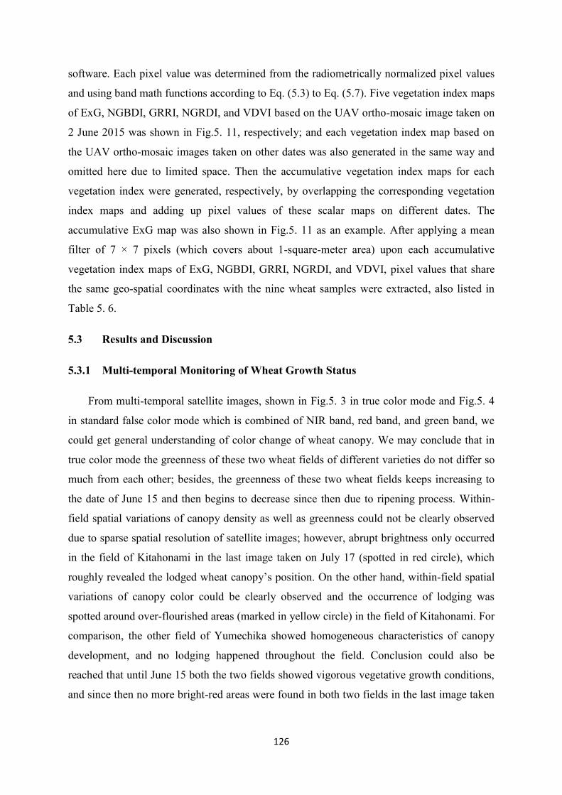
126

software. Each pixel value was determined from the radiometrically normalized pixel values

and using band math functions according to Eq. (5.3) to Eq. (5.7). Five vegetation index maps

of ExG, NGBDI, GRRI, NGRDI, and VDVI based on the UAV ortho-mosaic image taken on

2 June 2015 was shown in Fig.5. 11, respectively; and each vegetation index map based on

the UAV ortho-mosaic images taken on other dates was also generated in the same way and

omitted here due to limited space. Then the accumulative vegetation index maps for each

vegetation index were generated, respectively, by overlapping the corresponding vegetation

index maps and adding up pixel values of these scalar maps on different dates. The

accumulative ExG map was also shown in Fig.5. 11 as an example. After applying a mean

filter of 7 × 7 pixels (which covers about 1-square-meter area) upon each accumulative

vegetation index maps of ExG, NGBDI, GRRI, NGRDI, and VDVI, pixel values that share

the same geo-spatial coordinates with the nine wheat samples were extracted, also listed in

Table 5. 6.

5.3 Results and Discussion

5.3.1 Multi-temporal Monitoring of Wheat Growth Status

From multi-temporal satellite images, shown in Fig.5. 3 in true color mode and Fig.5. 4

in standard false color mode which is combined of NIR band, red band, and green band, we

could get general understanding of color change of wheat canopy. We may conclude that in

true color mode the greenness of these two wheat fields of different varieties do not differ so

much from each other; besides, the greenness of these two wheat fields keeps increasing to

the date of June 15 and then begins to decrease since then due to ripening process. Within-

field spatial variations of canopy density as well as greenness could not be clearly observed

due to sparse spatial resolution of satellite images; however, abrupt brightness only occurred

in the field of Kitahonami in the last image taken on July 17 (spotted in red circle), which

roughly revealed the lodged wheat canopy’s position. On the other hand, within-field spatial

variations of canopy color could be clearly observed and the occurrence of lodging was

spotted around over-flourished areas (marked in yellow circle) in the field of Kitahonami. For

comparison, the other field of Yumechika showed homogeneous characteristics of canopy

development, and no lodging happened throughout the field. Conclusion could also be

reached that until June 15 both the two fields showed vigorous vegetative growth conditions,

and since then no more bright-red areas were found in both two fields in the last image taken

127

about 10 days prior to harvesting on July 17, which indicated the dying-out process of wheat

canopies.

From UAV’s ortho-mosaic images straightforward visualization of wheat growth status

could be acquired. Within-field variations of wheat canopy density are so obvious that

existence of bare soil could even be noticed from the image taken on June 2. In terms of

time-domain, canopy greenness of both two wheat varieties reached peak value on June 10

2015, and there is no significant difference of canopy greenness between these two different

wheat varieties in early growth stages; however, from June 10 2015 it became very

distinctive that field No.2 (marked in red box) showed heavier canopy greenness compared

with the other one. In image taken on June 2 2015 of field No.1 (marked in black box) such

areas marked in circles had relatively higher level of stalk densities, and compounded with

other environmental influences such as rainfall, wind, and etc., it eventually led to the

occurrence of lodging at growth stage of grain-filling when the over-luxuriant canopies failed

to support heavy wheat ears, marked in image of July 16 and 24 2015. Fig.5. 12 showed a

close-shot photograph of the lodging spot in field No.1, taken on July 16 2015. It suggested

that UAV’s ortho-mosaic image taken from about one week ahead of harvesting could be

practically served as navigation references which guide either drivers of combine harvesters,

or autonomous harvesting vehicles, to adjust operation speed according to the specific

lodging situations for less loss rate of harvesting, as occurrence of lodging in wheat field has

been generally considered as the most influencing and direct factor which impairs the

working performance of combine harvester.

Fig.5. 12 Close-shot photograph of the lodging spot in test wheat field

128

Table 5. 7 Time-varying NDVI and VDVI values calculated from satellite images

Date Average Standard deviation

Satellite

NDVI

June 1 0.54 0.04

June 7 0.72 0.04

June 15 0.57 0.03

July 17 0.19 0.05

Satellite

VDVI

June 1 0.02 0.001

June 7 0.06 0.01

June 15 -0.01 0.02

July 17 0.003 0.02

Table 5. 8 Time-varying VDVI values calculated from UAV’s Ortho-mosaic images

Date Average Standard deviation

UAV

VDVI

June 2 0.12 0.01

June 10 0.15 0.02

June 19 0.08 0.03

June 25 0.14 0.02

July 2 0.10 0.02

July 10 0.10 0.01

July 16 0.06 0.01

July 24 0.02 0.01

In order to further analyze time-varying canopy color changes, the average values and

standard deviations of NDVI as well as VDVI samples derived out of each satellite image

were listed in Table 5. 7; and the average values and standard deviations of the corresponding

of VDVI samples based on each UAV ortho-mosaic image were listed Table 5. 8. The

increasing trend of satellite image based NDVI values was very clear at early growth stages,

and then NDVI values began to decrease stage by stage to minimum value around 0.19,

which was also showed in Fig.5. 13. On the other hand, VDVI values calculated from

satellite images suggested the same tendency with the NDVI counterpart that VDVI reached

maximum values on June 7 and then began to decrease as wheat changed from vegetative

growth into reproductive process. Besides, heavy variation of VDVI values derived from

satellite images around wheat ripening stage may be a big issue when used for quantitative

inversion with ground variables, showed in Fig.5. 13, as satellite image based VDVI is not as

reliable as NDVI when crops are in the process of ripening or yellowing and VDVI values

diverge around the threshold value of 0. Data on June 15 and July 17 indicated that most of

VDVI values were found to be negative numbers due to the interference of soil pixels

129

compounding with other reasons such as lodging, as the sparse resolution of satellite images

reaches up to about 5 m.

Fig.5. 13 Satellite image based vegetation indices

Fig.5. 14 UAV Ortho-mosaic image based VDVI

However, from the VDVI data based on UAV ortho-mosaic images, shown in Fig.5. 14,

we may conclude that the time-varying trend of VDVI based on the UAV ortho-mosaic

image is very alike with the one we made by observing multi-temporal changes of satellite

image based NDVI as well as satellite image based VDVI. Firstly VDVI values increased

until June 10 and then began to decrease stage by stage to the minimum value around 0.02.

The difference of UAV’s ortho-mosaic image based VDVI from satellite image based VDVI

is that the VDVI values of the former remote sensing source were found to be positive values

even until July 24, 2 day prior to harvesting, which once again confirmed VDVI’s capability

130

to differentiate vegetative areas from non-vegetative areas. The reason could be that

decimeter-level ground resolution of UAV’s ortho-mosaic images eliminated soil and other

background features’ interference. Nevertheless, the existence of abnormal value on 19 June

also indicated that the individual VDVI values based on a specific color image could be

deceptive, as it is not as reliable as the NDVI value due to the lack of NIR band.

Furthermore, correlation analysis of vegetation indices based on satellite images and

UAV’s ortho-mosaic images was performed for temporal complementation. All of four

satellite images and four out of eight UAV’s ortho-mosaic images that were taken temporally

around the dates of satellite images were used, from which vegetation indices were extracted,

respectively, as has been described in Sec. 5.2.3. Regression analysis showed that second-

order polynomial models fitted best between UAV’s Ortho-mosaic image based VDVI and

satellite image based VDVI as well as satellite image based NDVI, when compared with

other regression models such as linear, exponential, and power. Coefficient of determination

and RMSE were calculated as 0.62 and 0.019 for second-order polynomial regression model

between UAV’s ortho-mosaic image based VDVI and satellite image based VDVI. On the

other hand, coefficient of determination and RMSE were calculated as 0.58 and 0.127 for

second-order polynomial regression model between UAV’s ortho-mosaic image based VDVI

and satellite image based NDVI, respectively. Therefore, we may conclude that it is feasible

to temporally complement satellite remote sensing by using UAV’s ortho-mosaic images by

both visual interpretation and also quantitative analysis to monitor wheat growth status.

Fig.5. 15 Regression model between UAV images’ VDVI and satellite images’ VDVI

131

Fig.5. 16 Regression model between UAV images’ VDVI and satellite images’ NDVI

5.3.2 Mapping within-Field Variations of Wheat Yield

As mentioned in Sec.5.1, it was reported that accumulative vegetation indices values of

multi-temporal remote sensing images after flowering stage have good relationship with crop

yield. Besides, we have also understood from Sec.5.3.1 that vegetation index values from an

individual remote sensing image taken on a specific date could be inaccurate and deceptive

due to weather condition and etc. Therefore, in this study we conducted stepwise regression

analysis of sampled wheat yield with five different accumulative vegetation indices, which

were extracted from eight UAV’s ortho-mosaic images that covered a winter wheat field

from heading stage to ripening stage, as described in Sec.5.2.4. By using stepwise method, a

regression analysis was performed in MATLAB R2013a (The MathWorks, Inc.,Natick, MA,

USA) among the response variable of sampled wheat yield and five predictive variables of

accumulative vegetation indices of ExG, NGBDI, GRRI, NGRDI, and VDVI, listed in Table

5. 6.

The result of stepwise regression analysis showed that the variable of NGRDI was

removed from the stepwise regression model due to insignificant correlation with the

responsive variable of wheat yield, whilst the rest variable of VDVI, NGBDI, GRRI, and

ExG were included to fit the regression model expressed as Eq. (5.8), with coefficient of

determination as 0.94 and RMSE = 0.02. For comparison, the average value of sampled grain

yield was calculated as 0.86 kg per square meter. Subsequently, LOOCV was also conducted

132

by building nine linear regression models that uses eight set variables of sampled wheat yield

and values of VDVI, NGBDI, GRRI, and ExG as training data, whilst leaves one set of

variables as test data. RMSEP for the LOOCV was calculated as 0.06.

Y = −6.19−6.78 × X1 + 3.45 × X3 + 0.88 × X4 + 0.003 × X5 (5.8)

where Y, X1, X3, X4, and X5 denotes estimated wheat yield, accumulative VDVI, NGBDI,

GRRI, and ExG, respectively.

Based on the regression model expressed as Eq. (5.8), wheat yield was calculated by

using VDVI, NGBDI, GRRI, and ExG maps, and finally map of wheat yield was generated

accordingly in ENVI software. Wheat yield’s within-field spatial variations could be

observed from the yield map shown in Fig.5. 17 that non-uniformity of wheat yield of this

field is quite obvious and the occurrence of lodging coincide with the high-yield areas. By

observing the histogram of the wheat yield map we could also obtain the information that

about 25.8% areas in the studied field had grain weight per square meter below 0.5 kg, which

still has much room for improvement by implementing variable-rate fertilization, precise land

leveling, and etc.; whilst grain weight per square meter of most areas reached between 0.5–

1.5 kg, occupying about 50.4% acreages; and the average value of grain weight per square

meter was calculated as 0.72 kg, which indicated the estimated average yield of the studied

field as 7.2 t/ha. (The yield of Kitahonami planted in Hokkaido is reported from 6.0 to 8.5

t/ha year by year.)

Fig.5. 17 Map of wheat yield (expressed as grain weight per square meter).

133

Fig.5. 18 Histogram of wheat yield map

5.3 Conclusion

Based on the multi-temporal satellite remote sensing images and UAV’s ortho-mosaic

images, we monitored the time-varying canopy color change through image interpretation

and spotted the occurrence of wheat lodging from UAV ortho-mosaic images take from about

10 days prior to harvesting. It indicated that the high-resolution UAV ortho-mosaic image

could be used to guide drivers or autonomous harvesting vehicles to adjust operation speed

for less harvesting loss. Through monitoring changes of both satellite image based NDVI as

well as VDVI values and UAV’s ortho-mosaic image based VDVI values, conclusion was

reached that all of these three vegetation indices have the same and synchronized trend of

increasing at first, reaching up to peak values around June 7 or 10 2015 before wheat’s

reproductive growth begins, and starting to decrease since then. By observing the time-

varying values of vegetation indices, we concluded that UAV’s ortho-mosaic images with

high spatial resolution demonstrated good performance because pixel values are less affected

by background interference when compared with satellite images. We may also suggest that it

could be feasible of using commercial camera which is mounted upon small UAVs to

conduct both qualitative and quantitative study on crop monitoring.

We also analyzed the correlations among satellite remote sensing images based

vegetation indices and UAV’s ortho-mosaic image based vegetation index, to discuss the

Grain weight per square

meter

Fre

qu

ency

134

feasibility of utilizing UAV remote sensing images to temporarily complement satellite

remote sensing in case that satellite images were not available or cost-efficient over specific

areas. The correlation analysis of satellite image based NDVI as well as VDVI with UAV

ortho-mosaic image based VDVI showed good consistency at the early stage of wheat

growing season. However, at the late stage of wheat growing season VDVI based on satellite

images showed unreliable characteristics due to satellite image’s sparse spatial resolution; on

the other hand, VDVI based on UAV ortho-mosaic images fell rapidly to the values around

0.05 at the late growth stage and also showed very limited capability to differentiate wheat

growing status when compared with NDVI, due to the absence of the NIR band information.

Therefore, in order to remedy the confine of the direct use of UAV’s ortho-mosaic images,

image processing techniques such as image segmentation are considered to integrate UAV

ortho-mosaic images with satellite images in future work.

Through stepwise regression analysis of the response variable of sampled grain weight

per square meter and the predictive variables of accumulative color vegetation indices, we

can conclude that only the variable of normalized green-red difference index was removed

from the stepwise regression model due to insignificant p-value, whilst the rest variables of

visible-band difference vegetation index (the normalized green-blue difference index, green-

red ratio index, and excess green vegetation index) were included to fit the regression model,

with coefficient of determination and RMSE as 0.94 and 0.02, respectively. The averaged

value of sampled grain weight per square meter was calculated as 0.86 kg. The regression

model was also validated by using leave-one-out cross validation method, which showed that

the root-mean-square error of predication of the regression model was 0.06. Based on the

stepwise regression model, a map of estimated grain weight per square meter (yield map) was

generated and within-field spatial variations of wheat yield could be understood. The yield

map could be seen as the comprehensive presentation of the spatial variations of soil fertility,

tiller density, effective water potential, canopy aeration condition, and etc., which could be

used as reference for variable-rate fertilization and precise land-leveling in order to further

improve the overall yield.

135

Chapter 6 Summary

Agricultural remote sensing is a vital component of precision agriculture, which collects

and manifests the spatial variations of farmland condition and crop growth status for site-

specific treatments. Civilian applications of UAVs witnessed rapid development during these

two decades from recreational aerial photography to security monitoring, agricultural

spraying, remote sensing, and etc., due to advantages such like low cost, high efficiency,

good maneuverability, and safety. In this dissertation, we explored the feasibility of

introducing a low-altitude UAV as the platform into three agricultural remote sensing

projects including: (a). to generate topographic maps of farmland for precision land levelling

operation by integrating multiple sensors onboard the UAV platform; (b). to generate wheat

stalk density maps during the early growth stage for variable-rate topdressing by segmenting

UAV remote sensing images; and (c). to conduct correlation analysis between vegetation

indices based on UAV ortho-mosaic images and satellite remote sensing images, as well as to

map within-field spatial variations of wheat yield according to multi-temporal UAV remote

sensing images.

(a). A one-dimensional LiDAR distance measurement device was installed upon the

UAV platform, which is set to measure the distance between the ground surface to the UAV-

LiDAR system at the frequency of 10 Hz. The LiDAR distance measurements were amended

according to the UAV-LiDAR system’s attitude information, which were calculated from the

multiple MEMS IMU sensors incorporated inside the UAV’s flight controller. A PPK-GPS

module with small size and light weight features was also attached to the UAV-LiDAR

system, so that each LiDAR distance measurement could be geo-referenced and accordingly

the ground elevation of each surveying point could be calculated to acquire 3D coordinates

(latitude, longitude, and altitude). The static accuracies of LiDAR distance measurements and

the PPK-GPS positioning coordinates were validated by extracting 6000 sets of measuring

data, which indicated that the accuracy of LiDAR distance measurements is as high as 1cm,

whilst the horizontal and vertical accuracy of PPK-GPS is 1cm and about 2 cm, respectively.

The overall accuracy of the UAV-LiDAR system based topographic surveying approach was

also validated by using a RTK-GPS module to take 35 samples that uniformly spread

throughout the field under study and overlapped with the UAV-LiDAR system’s trajectory.

136

The RMSE between the ground elevation data of the UAV-LiDAR system and the validating

RTK-GPS altitude was calculated as 3.5 cm, which demonstrated high-accuracy and

feasibility of conducting topographic survey by using our proposed UAV-LiDAR system.

Visual inspection of the UAV-LiDAR system based topographic survey was also

implemented by manually building bumps and hollows inside the experimental field, and the

UAV-LiDAR system was found to be capable of clearly recognizing and demonstrating these

artificial features. Subsequently, different interpolation methods that were used to generate

farmland topographic maps based on the UAV-LiDAR system’s topographic surveying data

were investigated to select the most accurate interpolation model. As the result, TIN

interpolation model was found to be the most accurate one, and RMSE between the sampled

reference altitude values of RTK-GPS data and the corresponding ground elevation values of

the resulting topographic map based on TIN interpolation model was calculated as 13.7 cm.

Finally aerial photogrammetric DSM was integrated with the UAV-LiDAR system’s

topographic surveying data for an improved topographic map, as the former topographic data

has the advantage of large coverage but is also known for its unreliable accuracy, whist the

accuracy of the UAV-LiDAR system based topographic data is proved to be very high but the

spatial coverage is very poor. The RSME between the validating RTK-GPS altitude data and

the corresponding ground elevation values of the improved topographic map based on TIN

interpolation model was calculated as 5.9 cm, which showed great accuracy and practicability

of our proposed topographic mapping method.

(b). A multispectral camera (Green-Ren-NIR) was installed upon the UAV platform for

acquiring high-resolution images of wheat field during early growth stages. After ortho-

mosaicking and geo-referencing, the multispectral UAV images were transformed into a

NDVI map. Wheat stalk densities of the field under study were manually counted as ground

truth, of which the geographical coordinates were measured by using a RTK-GPS module.

The NDVI map was used to calculate FGV value, which is an indicator of the vegetation

coverage. Besides, the NDVI map was further binarized into vegetation class and background

class based on the conventional thresholding method as well as the SVM classifier method,

respectively; and VCC was calculated out of the classification result. Subsequently, different

regression models (linear, second-order polynomial, exponential, and power regression) were

built between the ground truth and the corresponding FGV and VCC, respectively. As the

result, we concluded that the regression models based on FGV have good accuracies with the

coefficient of determination around 0.89, whilst the regression models based on VCC have

137

better accuracies with the coefficient of determination around 0.94. Furthermore, we selected

the power regression model, which has the highest coefficient of determination of 0.95 and

root-mean-square error of 24, in consideration that the average value of the sampled stalk

densities was calculated as 593 stalks per square meter. The validating experiment on the

other wheat field with the same seeding rate and similar field management treatment also

confirmed that the power regression model is the most accurate and suitable model between

the sampled stalk density values and the SVM classifier based VCC values. Finally,

according to the power regression model 125 stalk density values were calculated by

extracting the corresponding VCC values from the resulting vegetation classification map

based on SVM classification method, and stalk density maps were generated by using

different interpolation methods. In thus, we would like to conclude that the UAV-camera

system could be used to obtain quantitative information for variable-rate topdressing in an

accurate and efficient manner.

(c). Agricultural application of UAV remote sensing by using commercial RGB cameras

decreases high cost of remote sensing sharply and provides instantly researchers and farmers

with actual and intuitive visualization of crop growth status, since color images accentuate

particular vegetation greenness and have been suggested to be less sensitive to variations of

illumination conditions. We installed a SONY ILCE-6000 commercial digital camera upon

the UAV platform and acquired 8 sets of RGB images over a wheat farmland, which were

further processed by generating and geo-referencing eight ortho-mosaic images. Based on the

multi-temporal (from early June to late July 2015) satellite remote sensing images on four

different dates and UAV’s ortho-mosaic images on eight different dates, we monitored the

time-varying canopy color change through image interpretation and spotted the occurrence of

wheat lodging from UAV ortho-mosaic images taken from about 10 days prior to harvesting.

It indicated that the high-resolution UAV ortho-mosaic image could be used to guide drivers

or autonomous harvesting vehicles to adjust operation speed for less harvesting loss

according to the specific lodging situations. We also analyzed the correlations among satellite

remote sensing images based vegetation indices and UAV’s ortho-mosaic image based

vegetation index, and the correlation analysis of satellite image based NDVI as well as VDVI

with UAV image based VDVI showed good consistency at the early stage of wheat growing

season. Through stepwise regression analysis of the response variable of sampled grain

weight per square meter and the predictive variables of accumulative color vegetation indices,

we can conclude that only the variable of normalized green-red difference index was

138

removed from the stepwise regression model due to insignificant p-value, whilst the rest

variables of visible-band difference vegetation index, the normalized green-blue difference

index, green-red ratio index, and excess green vegetation index were included to fit the

regression model, with coefficient of determination and RMSE as 0.94 and 0.02, respectively.

The averaged value of sampled grain weight per square meter was calculated as 0.86 kg. The

regression model was also validated by using leave-one-out cross validation method, which

showed that the RMSE of predication of the regression model was 0.06. Based on the

stepwise regression model, a map of estimated grain weight per square meter (yield map) was

generated and within-field spatial variations of wheat yield could be understood. The yield

map could be seen as the comprehensive presentation of the spatial variations of soil fertility,

tiller density, effective water potential, canopy aeration condition, and etc., which could be

used as reference for variable-rate fertilization and precise land-leveling in order to further

improve the overall yield.

In short, the UAV platform based agricultural remote sensing showed high accuracy and

efficiency in terms of the acquisition of field information, which is paramount for filling yield

gaps through site-specific farming techniques.

139

References

[1] United Nations News Centre – UN declares famine in another three areas of Somalia.

https://www.un.org/apps/news/story.asp?NewsID=39225&Cr=Somalia&Cr1=#.Wc2uyN

9Nxyx. Retrieved 2017-09-20.

[2] Hershey D. Misconceptions about Helmont’s willow experiment. Plant Science Bulletin.

2003; 49(3):78-84.

[3] Schell J. Stephen Hales and the cohesion theory.. Trends Plant Sci. 1999; 4(6):209.

[4] Brock, William H. Justus von Liebig: the chemical gatekeeper (1st ed.). 1997;

Cambridge, U.K.: Cambridge University Press. ISBN 9780521562249.

[5] McKeown, Thomas. The Modern Rise of Population. 1976; London, UK: Edward

Arnold. ISBN 9780713159868.

[6] Smil, Vaclav. Enriching the Earth: Fritz Haber, Carl Bosch, and the Transformation of

World Food Production. 2004; Cambridge, MA: MIT Press. ISBN 9780262693134.

[7] Hope from hybrid rice. http://www.chinadaily.com.cn/opinion/2011-

09/21/content_13745849.htm. Retrieved 2017-09-30.

[8] Population Division World Population Prospects 2017. https://esa.un.org/unpd/wpp/.

Retrieved 2017-09-30.

[9] Pimentel D, McLaughlin L, Zepp A, Lakitan B, Kraus T, Kleinman P, Vancini F, Roach

WJ, Graap E, Keeton WS, Selig G. Environmental and economic effects of reducing

pesticide use. BioScience. 1991 Jun 1;41(6):402-9.

[10] Digital agriculture: helping to feed a growing world. http://performance.ey.com/wp-

content/uploads/downloads/2017/02/EY-Performance-digital-agriculture.pdf. Retrieved

2017-09-30.

[11] Shibusawa, S., Anom, W.S., Sato, H., Sasao, A. On-line real-time soil

spectrophotometer. Proceedings of Fifth International Conference on Precision

Agriculture (CD), July 16 - 19, 2000. Bloomington, MN, USA.

[12] McBratney A, Whelan B, Ancev T, Bouma J. Future directions of precision agriculture.

Precision agriculture. 2005 Feb 1;6(1):7-23.

[13] Doerge T. Defining management zones for precision farming. Crop Insights.

1999;8(21):1-5.

[14] TECHNOLOGY ON THE FARM. https://www.arvigbusiness.com/technology-on-the-

farm/. Retrieved 2017-10-01.

140

[15] Stafford JV. Implementing precision agriculture in the 21st century. Journal of

Agricultural Engineering Research. 2000 Jul 1;76(3):267-75..

[16] Whelan BM, McBratney AB, Boydell BC. The impact of precision agriculture.

proceedings of the ABARE outlook conference. The Future of Cropping in NW NSW,

Moree, UK. 1997 Jul:5.

[17] John E. Sawyer. Making every fertilizer dollar pay. Presented at the 11th annual

Integrated Crop Nutrient Management Conference, p. 63-78. Dec. 1-2, 1999. Iowa State

University, Ames, IA.

[18] Wagner LE, Schrock MD. Yield determination using a pivoted auger flow sensor.

Transactions of the ASAE. 1989;32(2):409-0413..

[19] Yule IJ, Kohnen G, Nowak M. A tractor performance monitor with DGPS capability.

Computers and Electronics in Agriculture. 1999 Aug 31;23(2):155-74.

[20] Tian L, Reid JF, Hummel JW. Development of a precision sprayer for site-specific weed

management. Transactions of the ASAE. 1999;42(4):893.

[21] Hummel JW, Sudduth KA, Hollinger SE. Soil moisture and organic matter prediction of

surface and subsurface soils using an NIR soil sensor. Computers and electronics in

agriculture. 2001 Aug 31;32(2):149-65.

[22] Noguchi N, Reid JF, Zhang Q, Will JD, Ishii K. Development of robot tractor based on

RTK-GPS and gyroscope. In2001 ASAE Annual Meeting 1998 (p. 1). American Society

of Agricultural and Biological Engineers.

[23] Misra P, Enge P. Global Positioning System: signals, measurements and performance

second edition. Massachusetts: Ganga-Jamuna Press. 2006.

[24] Chang, K. T. Introduction to Geographical Information Systems. New York: McGraw

Hill. 2008.

[25] Panigrahi N. Computing in geographic information systems. CRC Press; 2014 Jul 10.

[26] Lillesand T, Kiefer RW, Chipman J. Remote sensing and image interpretation. John

Wiley & Sons; 2014 Dec 31.

[27] Mulla DJ. Twenty five years of remote sensing in precision agriculture: Key advances

and remaining knowledge gaps. Biosystems engineering. 2013 Apr 30;114(4):358-71.

[28] Colwell R. Determining the prevalence of certain cereal crop diseases by means of aerial

photography. California Agriculture. 1956 Nov 1;26(5):223-86.

[29] Eisenbeiss H. A mini unmanned aerial vehicle (UAV): system overview and image

acquisition. International Archives of Photogrammetry. Remote Sensing and Spatial

Information Sciences. 2004 Nov 18;36(5/W1):1-7.

141

[30] K J Stout; L Blunt. Three Dimensional Surface Topography, 2nd ed.; Penton Press:

London, England, 2000; pp. 3-7.

[31] Geographical Information System. Available online:

http://www.michigan.gov/cgi/0,1607,7-158-14767-318 93--F,00.html (accessed on 8

September 2017).

[32] Levidow L, Zaccaria D, Maia R, Vivas E, Todorovic M, Scardigno A. Improving water-

efficient irrigation: Prospects and difficulties of innovative practices. Agricultural Water

Management. 2014 Dec 31;146:84-94..

[33] Hu Lian, Luo Xiwen, et al. Development of 1PJ-4. 0 Laser Leveler Installed on a

Wheeled Tractor for Paddy Field. Transactions of the Chinese Society for Agricultural

Machinery, 2014, 45, 146-151. (in Chinese)

[34] Rickman, J.F., 2002. Manual for laser land levelling, Rice-Wheat Consortium Technical

Bulletin Series 5. New Delhi-110 012, India: Rice-Wheat Consortium for the Indo-

Gangetic Plains. pp. 24.

[35] Hamid Raeisi-Vanani, Mohammad Shayannejad, et al. A Simple Method for Land

Grading Computations and its Comparison with Genetic Algorithm (GA) Method.

International Journal of Research Studies in Agricultural Sciences, 2017, 3, 8, pp 26-38.

[36] Agricultural Land Levelling. Available online: http://www.optisurface.com/agricultural-

land-levelling/.

[37] Jat ML, Chandna P, Gupta R, Sharma SK, Gill MA. Laser land leveling: a precursor

technology for resource conservation. Rice-Wheat consortium technical bulletin series.

2006;7:48.

[38] Yongjian L, Zuoxi Z. Design of Attitude Measurement System for Flat Shovel of Laser-

controlled Land Leveler for Paddy Field [J]. Journal of Agricultural Mechanization

Research. 2012;2:69-75..

[39] Zimmerman, Kurt R., et al. System and method for land-levelling. U.S. Patent No

6,880,643, 2005.

[40] Johnson KM, Ouimet WB. Rediscovering the lost archaeological landscape of southern

New England using airborne light detection and ranging (LiDAR). Journal of

Archaeological Science. 2014 Mar 31;43:9-20.

[41] Bosse M, Zlot R, Flick P. Zebedee: Design of a spring-mounted 3-d range sensor with

application to mobile mapping. IEEE Transactions on Robotics. 2012 Oct;28(5):1104-19.

[42] Remondino F. Heritage recording and 3D modeling with photogrammetry and 3D

scanning. Remote Sensing. 2011 May 30;3(6):1104-38..

142

[43] Moskal LM, Zheng G. Retrieving forest inventory variables with terrestrial laser

scanning (TLS) in urban heterogeneous forest. Remote Sensing. 2011 Dec 23;4(1):1-20.

[44] Zhang S, Wang C, Yang Z, Chen Y, Li J. Automatic railway power line extraction using

mobile laser scanning data. Proceedings of the International Archives of the

Photogrammetry, Remote Sensing and Spatial Information Sciences, Prague, Czech

Republic. 2016 Jul 12;5:615-9.

[45] Guo Zong-he, Zheng Jin-feng, Cui Yun-chuan. Surveying and Setting-out Based on

Two-point Reference Line with Total Station. Bulletin of Surveying and Mapping, 2004,

8: 022.

[46] Resop JP, Hession WC. Terrestrial laser scanning for monitoring streambank retreat:

Comparison with traditional surveying techniques. Journal of Hydraulic Engineering.

2010 Mar 27;136(10):794-8.

[47] Corsini A, Castagnetti C, Bertacchini E, Rivola R, Ronchetti F, Capra A. Integrating

airborne and multi‐ temporal long‐ range terrestrial laser scanning with total station

measurements for mapping and monitoring a compound slow moving rock slide. Earth

surface processes and landforms. 2013 Sep 15;38(11):1330-8.

[48] Rodríguez-Gonzálvez P, Jiménez Fernández-Palacios B, Muñoz-Nieto ÁL, Arias-

Sanchez P, Gonzalez-Aguilera D. Mobile LiDAR System: New Possibilities for the

Documentation and Dissemination of Large Cultural Heritage Sites. Remote Sensing.

2017 Feb 23;9(3):189.

[49] Hirano A, Welch R, Lang H. Mapping from ASTER stereo image data: DEM validation

and accuracy assessment. ISPRS Journal of Photogrammetry and Remote Sensing. 2003

Apr 30;57(5):356-70.

[50] Harwin S, Lucieer A. Assessing the accuracy of georeferenced point clouds produced

via multi-view stereopsis from unmanned aerial vehicle (UAV) imagery. Remote

Sensing. 2012 May 30;4(6):1573-99.

[51] Lovitt J, Rahman MM, McDermid GJ. Assessing the Value of UAV Photogrammetry

for Characterizing Terrain in Complex Peatlands. Remote Sensing. 2017 Jul 12;9(7):715.

[52] Goyer GG, Watson R. The laser and its application to meteorology. Bulletin of the

American Meteorological Society. 1963 Sep;44(9):564-75.

[53] Artale V, Milazzo CL, Ricciardello A. Mathematical modeling of hexacopter. Appl.

Math. Sci. 2013;7(97):4805-11..

[54] Huang YP. Triangular irregular network generation and topographical modeling.

Computers in industry. 1989 Jul 1;12(3):203-13.

143

[55] Peucker TK, Fowler RJ, Little JJ, Mark DM. The triangulated irregular network. InAmer.

Soc. Photogrammetry Proc. Digital Terrain Models Symposium 1978 May 9 (Vol. 516, p.

532).

[56] Tsai VJ. Delaunay triangulations in TIN creation: an overview and a linear-time

algorithm. International Journal of Geographical Information Science. 1993 Nov

1;7(6):501-24.

[57] Philip, G. M., and D. F. Watson. A Precise Method for Determining Contoured Surfaces.

Australian Petroleum Exploration Association Journal 22: 205–212. 1982.

[58] Watson, D. F., and G. M. Philip. A Refinement of Inverse Distance Weighted

Interpolation. Geoprocessing 2:315–327. 1985.

[59] Franke R. Smooth interpolation of scattered data by local thin plate splines. Computers

& Mathematics with Applications. 1982 Jan 1;8(4):273-81.

[60] Mitáš L, Mitášová H. General variational approach to the interpolation problem.

Computers & Mathematics with Applications. 1988 Jan 1;16(12):983-92.

[61] Aurenhammer F. Voronoi diagrams—a survey of a fundamental geometric data

structure. ACM Computing Surveys (CSUR). 1991 Sep 1;23(3):345-405.

[62] Sibson, R. A Brief Description of Natural Neighbor Interpolation, chapter 2 in

Interpolating Multivariate Data. New York: John Wiley & Sons, 1981. 21–36.

[63] LI, Zhilin; ZHU, Christopher; GOLD, Chris. Digital terrain modeling: principles and

methodology. CRC press, 2004.

[64] Global wheat production from 1990/1991 to 2016/2017 (in million metric tons).

https://www.statista.com/statistics/267268/production-of-wheat-worldwide-since-1990/.

Retrieved October 20, 2016.

[65] Shewry PR, Hey SJ. The contribution of wheat to human diet and health. Food and

Energy Security. 2015, 4 (3): 178–202.

[66] CURTIS, Byrd C., et al. Bread wheat: improvement and production. Food and

Agriculture Organization of the United Nations (FAO), 2002.

[67] Zadoks J C., Chang T T., Konzak C F. A decimal code for the growth stages of cereals.

Weed Res. 1974, 14, 415-21.

[68] Nick Poole. Cereal growth stages. Grains research & development corporation, New

Zealand, 2005; pp. 4-40.

[69] Small Grain Production Guide Revised March 2013,

http://www.smallgrains.ncsu.edu/production-guide.html (accessed 2015.05.01).

144

[70] Clement Atzberger. Advances in Remote Sensing of Agriculture: Context Description,

Existing Operational Monitoring Systems and Major Information Needs. Remote Sens.

2013, 5, 949-981.

[71] Irene Aicardi, Francesco Nex, Markus Gerke and Andrea Maria Lingua. An Image-

Based Approach for the Co-Registration of Multi-Temporal UAV Image Datasets.

Remote Sens. 2016, 8, 779.

[72] Colewell, R.N. Determining the prevalence of certain cereal crop diseases by means of

aerial photography. Hilgardia 1956, 26, 223-286.

[73] Huang Y, Thomson S J, Brand H J, Reddy K N. Development of low-altitude remote

sensing systems for crop production management. Int J Agric & Biol Eng. 2016, 9(4): 1-

11.

[74] Lu B, He Y. Species classification using Unmanned Aerial Vehicle (UAV)-acquired high

spatial resolution imagery in a heterogeneous grassland. ISPRS Journal of

Photogrammetry and Remote Sensing. 2017 Jun 30;128:73-85.

[75] Wang Xiaoqin, Wang Miaomiao, Wang Shaoqiang, Wu yundong. Extraction of

vegetation information from visible unmanned aerial vehicle images. Transactions of

Chinese Society of Agriculture Engineering 2015, 31(5):152-159.

[76] Rasmussen, J.; Ntakos, G.; Nielsen, J.; Svensgaard, J.; Poulsen, R. N.; Christensen, S.

Are vegetation indices derived from consumer-grade cameras mounted on UAVs

sufficiently reliable for assessing experimental plots? European Journal of Agronomy

2016, 74, 75–92.

[77] City of Sapporo. http://www.city.sapporo.jp/city/aramashi/ (Retrieved October 25,

2016).

[78] LebourgeoisV., BéguéA., LabbéS., MallavanB., PrévotL., Roux B., 2008. Can

commercial digital cameras be used as multispectral sensors? A crop monitoring test.

Sensors, 7300-7322.

[79] Bobbe, T.; McKean, J.; Zigadlo, J.P. An evaluation of natural color and color infrared

digital cameras as a remote sensing tool for natural resource management. Airborne

Reconnaissance XIX; Bellingham, WA, USA, 1995; Volume 2555, pp. 151-157.

[80] Rouse, J. W., R. H. Haas, J. A. Schell, and D. W. Deering, 1973. Monitoring vegetation

systems in the Great Plains with ERTS, Third ERTS Symposium, NASA SP-351 I, 309-

317.

145

[81] Kriegler, F.J., Malila, W.A., Nalepka, R.F., and Richardson, W. (1969) 'Preprocessing

transformations and their effects on multispectral recognition.' Proceedings of the Sixth

International Symposium on Remote Sensing of Environment, p. 97-131.

[82] Crippen, R.E. (1990) 'Calculating the vegetation index faster,' Remote Sensing of

Environment, 34, 71-73.

[83] Li X, Zhang J. Derivation of the green vegetation fraction of the whole China from 2000

to 2010 from MODIS data. Earth Interactions. 2016 Mar;20(8):1-6.

[84] Song W, Mu X, Ruan G, Gao Z, Li L, Yan G. Estimating fractional vegetation cover

and the vegetation index of bare soil and highly dense vegetation with a physically based

method. International Journal of Applied Earth Observation and Geoinformation. 2017

Jun 30;58:168-76.

[85] Purcell LC. Soybean canopy coverage and light interception measurements using digital

imagery. Crop Science. 2000 May 1;40(3):834-7.

[86] Korhonen, L., Korpela, I., Heiskanen, J. and Maltamo, M., 2011. Airborne discrete-

return LIDAR data in the estimation of vertical canopy cover, angular canopy closure

and leaf area index. Remote Sensing of Environment, 115(4), pp.1065-1080.

[87] Iosif VOROVENCII, Mihaela Denisa MUNTEAN. Evaluation of Supervised

Classification Algorithms for Landsat 5 TM Images, RevCAD. 2013, 14, 197-206.

[88] KEARNS, Michael; RON, Dana. Algorithmic stability and sanity-check bounds for

leave-one-out cross-validation. Neural computation, 1999, 11.6: 1427-1453.

[89] FENG Qisheng, GAO Xinhua. Application of Excel in the Experiment Teaching of

Leave-One-Out Cross Validation. Experiment Science and Technology, 2015, 13.2: 49-

51.

[90] Wu, Q.; Wang, C.; Fang, J.J.; Ji, J.W. Field monitoring of wheat seedling stage with

hyperspectral imaging. Int. J. Agric. Biol. Eng. 2016, 9, 143–148.

[91] Zhang, F.; Wu, B.; Luo, Z. Winter wheat yield predicting for America using remote

sensing data. J. Remote Sens. 2004, 8, 611–617.

[92] Roberto, B.; Paolo, R. On the use of NDVI profiles as a tool for agricultural statistics:

The case study of wheat yield estimate and forecast in Emilia Romagna. Remote Sens.

Environ. 1993, 45, 311–326, doi:10.1016/0034-4257(93)90113-C.

[93] Du X, Wu B, Li Q, Meng J, Jia K. A method to estimated winter wheat yield with the

MERIS data. InProgress in Electromagnetics Research Symposium (PIERS) Proceedings.

Beijing, China. March 23Á27 2009 Mar 23.

146

[94] Okuno R. Wheat Harvest Support System to Optimize Harvest Timing with Satellite

Remote-sensing. JOURNAL of the JAPANESE SOCIETY of AGRICULTURAL

MACHINERY. 2005 Sep 1;67(5):17-9.

[95] Han-ya I, Ishii K, Noguchi N. Estimation of moisture content of wheat ear using satellite

and helicopter imagery. Pap. Environ. Inf. Sci. 2009;23:155-60.

[96] Reyns P, Missotten B, Ramon H, De Baerdemaeker J. A review of combine sensors for

precision farming. Precision Agriculture. 2002 Jun 1;3(2):169-82.

[97] Space engineering development Co., Ltd., WorldView-2.

http://www.sed.co.jp/sug/contents/satellite/satellite_worldview2.html. Accessed on 2016-12-

05.

[98] Satellite image corporation, RapidEye Satellite Sensor.

http://www.satimagingcorp.com/satellite-sensors/other-satellite-sensors/rapideye/.

Accessed on 2016-12-05.

[99] Ministry of Agriculture, Forestry and Fisheries, Statistics on farmland.

http://www.maff.go.jp/j/tokei/sihyo/data/10.html. Accessed on 2017-11-25.

[100] Du M M, Noguchi N. Monitoring of wheat growth status and mapping of wheat

yield’s within-field spatial variations using color images acquired from UAV-camera

system. Remote Sensing, 2017; 9(3): 289.

[101] Campbell J B, Wynne R H. Introduction to remote sensing. 5th edition. The

Guilford Press, New York, USA, 2011; pp.72–102.

[102] Wang X Q, Wang M M, Wang S Q, Wu Y D. Extraction of vegetation information

from visible unmanned aerial vehicle images. Transactions of the CSAE, 2015; 31(5):

152–159.

[103] Hunt E R, Hively J W D, Fujikawa S J, Linden D S, Daughtry C S T, McCarty G W.

Acquisition of NIR-green-blue digital photographs from unmanned aircraft for crop

monitoring. Remote Sens, 2010; 2: 290–305.

[104] Torres-Sánchez J, López-Granados F, De Castro A I, Peña-Barragán J M.

Configuration and specifications of an unmanned aerial vehicle (UAV) for early site

specific weed management. PLoS One, 2013; 8(3): e58210.

[105] Woebbecke D M, Meyer G E, Von Bargen K, Mortensen D A. Color indices for

weed identification under various soil, residue and lighting conditions. Transactions of

the ASAE 1995; 38(1): 259–269.

147

[106] Cui, R.X.; Liu, Y.D.; Fu, J.D. Estimation of winter wheat biomass using visible

spectral and BP based artificial neural networks. Spectrosc. Spectr. Anal. 2015, 35,

2596–2601.

[107] http://www.data.jma.go.jp/obd/stats/etrn/view/annually_a.php?prec_no=20&block_no

=0115&year=2015&month=&day=&view=p1. Accessed on 2017-05-20.

[108] MAFF. http://www.maff.go.jp/. Accessed on 2016-11-10.

[109] Chander G, Haque M O, Sampath A, Brunn A, Trosset G, Hoffmann D, et al.

Radiometric and geometric assessment of data from the RapidEye constellation of

satellites, International Journal of Remote Sensing, 2013; 34(16): 5905–5925.

[110] Vermote, E. F., Tanre, D., Deuze, J. L., Herman, M., and Morcrette, J.-J, 1997.

Second Simulation of the Satellite Signal in the Solar Spectrum, 6S: an overview, IEEE

T. Geosci. Remote, 35, 675–686.

[111] Berk, A., Bernstein, L., and Robertson, D, 1989. MODTRAN: a moderate resolution

model for LOWTRAN7, Tech. Rep. GL-TR-89-0122, Air Force Geophysics Lab,

Hanscom AFB, Massachusetts, USA.

[112] de Carvalho OA, Guimarães RF, Silva NC, Gillespie AR, Gomes RA, Silva CR, de

Carvalho AP. Radiometric normalization of temporal images combining automatic

detection of pseudo-invariant features from the distance and similarity spectral measures,

density scatterplot analysis, and robust regression. Remote Sensing. 2013 May

30;5(6):2763-94..

148

List of Publications

Journal Paper

1. Du M, Noguchi N, Okamoto H, Kobayashi N. Topographic Mapping of Farmland by

Integration of Multiple Sensors on Board Low-Altitude Unmanned Aerial System.

World Academy of Science, Engineering and Technology, International Journal of

Computer and Systems Engineering. 2017 Nov 13;4(11).

2. Du M, Noguchi N. Monitoring of Wheat Growth Status and Mapping of Wheat

Yield’s within-Field Spatial Variations Using Color Images Acquired from UAV-

camera System. Remote Sensing. 2017 Mar 21;9(3):289.

3. Du M, Noguchi N, Atsushi I, Yukinori S. Multi-temporal monitoring of wheat growth

by using images from satellite and unmanned aerial vehicle. International Journal of

Agricultural and Biological Engineering. 2017 Sep 30;10(5):1-3.

Proceeding of Conference

1. Du M, Noguchi N. Multi-temporal Monitoring of Wheat Growth through Correlation

Analysis of Satellite Images, Unmanned Aerial Vehicle Images with Ground Variable.

IFAC-PapersOnLine. 2016 Dec 31;49(16):5-9.