Agilent 6200 Series TOF and 6500 Series Q-TOF LC/MS … · puter Software Documentation). Safety...
139
Agilent 6200 Series TOF and 6500 Series Q-TOF LC/MS System Concepts Guide The Big Picture
Transcript of Agilent 6200 Series TOF and 6500 Series Q-TOF LC/MS … · puter Software Documentation). Safety...
Agilent 6200 Series TOF and 6500 Series Q-TOF LC/MS System
Concepts Guide
The Big Picture
Notices© Agilent Technologies, Inc. 2017
No part of this manual may be reproduced in any form or by any means (including electronic storage and retrieval or transla-tion into a foreign language) without prior agreement and written consent from Agi-lent Technologies, Inc. as governed by United States and international copyright laws.
Manual Part Number
G3335-90231
Edition
Revision A, April 2017
Agilent Technologies, Inc.5301 Stevens Creek Blvd. Santa Clara, CA 95051
Warranty
The material contained in this docu-ment is provided “as is,” and is sub-ject to being changed, without notice, in future editions. Further, to the max-imum extent permitted by applicable law, Agilent disclaims all warranties, either express or implied, with regard to this manual and any information contained herein, including but not limited to the implied warranties of merchantability and fitness for a par-ticular purpose. Agilent shall not be liable for errors or for incidental or consequential damages in connection with the furnishing, use, or perfor-mance of this document or of any information contained herein. Should Agilent and the user have a separate written agreement with warranty terms covering the material in this document that conflict with these terms, the warranty terms in the sep-arate agreement shall control.
Technology Licenses
The hardware and/or software described in this document are furnished under a license and may be used or copied only in accordance with the terms of such license.
Restricted Rights Legend
U.S. Government Restricted Rights. Soft-ware and technical data rights granted to the federal government include only those rights customarily provided to end user cus-tomers. Agilent provides this customary commercial license in Software and techni-cal data pursuant to FAR 12.211 (Technical Data) and 12.212 (Computer Software) and, for the Department of Defense, DFARS 252.227-7015 (Technical Data - Commercial Items) and DFARS 227.7202-3 (Rights in Commercial Computer Software or Com-puter Software Documentation).
Safety Notices
CAUTION
A CAUTION notice denotes a haz-
ard. It calls attention to an operat-
ing procedure, practice, or the like
that, if not correctly performed or
adhered to, could result in damage
to the product or loss of important
data. Do not proceed beyond a
CAUTION notice until the indi-
cated conditions are fully under-
stood and met.
WARNING
A WARNING notice denotes a
hazard. It calls attention to an
operating procedure, practice, or
the like that, if not correctly per-
formed or adhered to, could result
in personal injury or death. Do not
proceed beyond a WARNING
notice until the indicated condi-
tions are fully understood and
met.
Software Revision
This guide applies to the Agilent MassHunter Workstation Software – Data Acquisition program for TOF and Q-TOF ver-sion B.08.01or higher until superseded.
In This Guide...
The Concepts Guide presents “The Big Picture” behind the Agilent TOF and Q-TOF LC/MS system to help you analyze samples on your Agilent time-of-flight or quadrupole time-of-flight mass spectrometer system. This guide helps you understand how the hardware and software work together.
1 Overview
Learn how the Agilent 6200 Series TOF and 6500 Series Q-TOF LC/MS system helps you do your job and how the hardware and software work.
2 Instrument Preparation
Learn the concepts you need to prepare the instrument for sample acquisition.
3 Methods with Acquisition Parameters
Learn concepts to help you enter instrument control parameter values and set up methods with acquisition parameters.
4 Data Acquisition
Learn concepts to help you enter information to run individual samples or a worklist of samples, and to help you acquire data and monitor runs.
Agilent 6200 Series TOF and 6500 Series Q-TOF LC/MS System Concepts Guide 3

4 Agilent 6200 Series TOF and 6500 Series Q-TOF LC/MS System Concepts Guide
Content
1 Overview
How does the TOF and Q-TOF system help you do your job? 10
Help for applications 11Help for data acquisition 11Help for data analysis 13
How do different ion sources work? 16
Electrospray ionization (ESI) and Dual ESI 17Dual Agilent Jet Stream Electrospray Ionization (Dual AJS
ESI) 21Atmospheric pressure chemical ionization (APCI) 22Atmospheric pressure photoionization (APPI) 24Multimode ionization (MMI) 25
How does the Agilent TOF and Q-TOF mass spectrometer work? 27
Innovative Enhancements in the 6545XT AdvanceBio Q-TOF 34
Innovative Enhancements in the 6560 Ion Mobility Q-TOF 35Innovative Enhancements in the 6550 iFunnel Q-TOF 36Innovative Enhancements in the 6545 Q-TOF 38Innovative Enhancements in the 6540 and 6538 Q-TOF 39Innovative Enhancements in the 6530 Q-TOF 41Agilent Jet Stream Thermal Gradient Source 42Front-end ion optics 44
2 Instrument Preparation
LC preparation 52
LC module setup 52Column equilibration and conditioning 55
TOF and Q-TOF preparation – calibration and tuning 57
Agilent 6200 Series TOF and 6500 Series Q-TOF LC/MS System Concepts Guide 5
TOF mass calibration 58Tuning choices 60Tune reports 71Storage and retrieval of tune results and Instrument Mode 72Tune Set Point Modifications for Medium and Large
Proteins 74
Real-time displays 75
Instrument Status Window 75Real-time parameter values (Actuals) 76Real-time Chromatogram Plot and Spectral Plot windows 78
System logbook 80
3 Methods with Acquisition Parameters
Parameter entry 84
LC parameter entry 84TOF and Q-TOF parameter entry 84Automatic TOF and Q-TOF parameter changes during a run 85Acquisition tab 86General TOF and Q-TOF parameters 87Ion source parameters 89TOF and Q-TOF acquisition parameters 91Setup of TOF and Q-TOF reference mass correction
(recalibration) 100TOF and Q-TOF chromatogram setup 104Q-TOF Advanced Parameters for Ion Mobility 105Setting parameters to acquire a data file in All Ions MS/MS
mode 108Setting parameters on a 6560 IM-QTOF to acquire a data file in
All Ions MS/MS mode 111
Method saving, editing and reporting 112
Saving a method with data acquisition parameters 112Method editing 114
6 Agilent 6200 Series TOF and 6500 Series Q-TOF LC/MS System Concepts Guide
Method reporting 115
4 Data Acquisition
Interactive single sample setup 118
Sample information 118Data File information 119Some of the Additional Information parameters 119
Worklist setup 120
Worklist menus 121Sample entry 122Script entry 124Entry of additional sample information (show, add
columns) 125Worklist import 126Report setup 130Run setup 131Estimate of worklist file size 132
Data acquisition for samples and worklists 136
What you can monitor during a run 136What you can do during a run 137
Agilent 6200 Series TOF and 6500 Series Q-TOF LC/MS System Concepts Guide 7

This page intentionally left blank.
8 Agilent 6200 Series TOF and 6500 Series Q-TOF LC/MS System Concepts Guide
Agilent 6200 Series TOF and 6500 Series Q-TOF LC/MS System
1Overview
How does the TOF and Q-TOF system help you do your job? 10
Help for applications 11
Help for data acquisition 11
Help for data analysis 13
How do different ion sources work? 16
Electrospray ionization (ESI) and Dual ESI 17
Dual Agilent Jet Stream Electrospray Ionization (Dual AJS ESI) 21
Atmospheric pressure chemical ionization (APCI) 22
Atmospheric pressure photoionization (APPI) 24
Multimode ionization (MMI) 25
How does the Agilent TOF and Q-TOF mass spectrometer work? 27
Innovative Enhancements in the 6545XT AdvanceBio Q-TOF 34
Innovative Enhancements in the 6560 Ion Mobility Q-TOF 35
Innovative Enhancements in the 6550 iFunnel Q-TOF 36
Innovative Enhancements in the 6540 and 6538 Q-TOF 39
Innovative Enhancements in the 6530 Q-TOF 41
Agilent Jet Stream Thermal Gradient Source 42
Front-end ion optics 44
This chapter provides an overview of the Agilent 6200 Series TOF LC/MS and Agilent 6500 Series Q-TOF LC/MS systems and the system components and how they work together to help you get your job done.
9
1 Overview
How does the TOF and Q-TOF system help you do your job?
How does the TOF and Q-TOF system help you do your job?
You can set up an Agilent 6200 Series Time-of-Flight LC/MS (TOF) system and the Agilent 6500 Series Quadrupole Time-of-Flight LC/MS (Q-TOF) system in several configurations:
ESI – Electrospray Ionization
APCI – Atmospheric Pressure
Chemical Ionization
APPI - Atmospheric Pressure
Photo Ionization
MALDI – Matrix-Assisted Laser
Desorption Ionization
MMI - Multimode Ionization
• For normal flow LC/MS with a binary pump, quaternary pump, well-plate sampler (or autosampler or HTC/HTS autosampler) and ESI or Dual ESI with Agilent Jet Stream Thermal Gradient Source - 6530 Quadrupole Time-of-Flight, 6540 Quadrupole Time-of-Flight, 6545 Quadrupole Time-of-Flight, 6545XT AdvanceBio Quadrupole Time-of-Flight, 6550 iFunnel Quadrupole Time-of-Flight, 6560 Ion Mobility Quadrupole Time-of-Flight, and 6230 Time-of-Flight.
• For normal flow LC/MS with a binary pump, quaternary pump, well-plate sampler (or autosampler or HTC/HTS autosampler) and ESI, Dual ESI, APCI, APPI, or MMI ion sources.
• For microflow LC/MS with a capillary pump, micro well-plate sampler and ESI, Dual ESI, APCI or MMI ion sources.
• For nanoflow LC/MS with a nanopump, micro well-plate sampler and nano-ESI source to increase reliability and boost performance with narrow peak dispersion and lower dead volumes.
• 6200 Series TOF or 6500 Series Q-TOF LC/MS system with an AP-MALDI or PDF-MALDI source.
Each Agilent system has advantages for high throughput sample screening with highly sensitive detection and accurate mass assignment. Each uses the same 6200 Series TOF or 6500 Series Q-TOF LC/MS software to enable these advantages.
The 6530, 6540, 6545, 6545XT, 6550, and the 6560 Q-TOF instruments can all use the Agilent Jet Stream source. The 6230 is the only TOF that can use the Agilent Jet Stream source. This source uses a super-heated sheath gas to collimate the nebulizer spray which dramatically increases the number of ions that enter the mass spectrometer.
10 Agilent 6200 Series TOF and 6500 Series Q-TOF LC/MS System Concepts Guide
Overview 1
Help for applications
Help for applications
You can use one or more of the 6200 Series TOF or 6500 Series Q-TOF LC/MS systems in the following application areas (for example):
• Combinatorial chemistry target compound analysis
• Natural products screening
• Compound profiling (such as bioavailability and pK)
• Protein/peptide identification and characterization
• Metabolomics
• Biomarker discovery
• Impurity profiling
Paired with Agilent Infinity and Infinity II Series LCs, the 6500 Series Q-TOF LC/MS delivers fast, sensitive, reproducible analyses of small and large molecules.
• Reproducible mass accuracy
• Ultra-trace limits of detection
• Fast MS/MS operation (for the Q-TOF)
Help for data acquisition
Please refer to this guide, the Agilent MassHunter Workstation Software - Data Acquisition Familiarization Guide, the Agilent MassHunter Workstation Software - Data Acquisition Quick Start Guide, the Data Acquisition for TOF/Q-TOF eFamiliarization Guide, or the online Help for the Data Acquisition program.
To help you use the 6200 Series TOF and the 6500 Series Q-TOF LC/MS systems for these applications, the software lets you perform the following tasks in a single window:
Agilent 6200 Series TOF and 6500 Series Q-TOF LC/MS System Concepts Guide 11
1 Overview
Help for data acquisition
Prepare the instrument
To learn how to get started with
the 6200 Series TOF and 6500
Series Q-TOF, see the Quick Start
Guide.
To learn more about how to use
the 6200 Series TOF and 6500
Series Q-TOF with real samples
and data, see the Familiarization
Guide or the eFamiliarization
Guide.
To learn how to perform individual
tasks with the TOF and Q-TOF
LC/MS, see the online Help. Press
F1 to access the online Help.
To learn more about an 1100 or
1200 LC module or 1260 or 1290
Infinity LC module or 1260 Infinity
II module, see the 1100 LC, 1200
LC, 1260 Infinity LC, 1260 Infinity II,
or 1290 Infinity LC User Guide for
the module.
To learn more about the 6200
Series TOF or the 6500 Series
Q-TOF, see the Maintenance Guide
(Animated).
To learn how to install the system,
see the Installation Guide.
• Start and stop the instruments from the software.
• Download settings to the 1100, 1200, 1260 Infinity or 1290 Infinity liquid chromatograph and the TOF and Q-TOF mass spectrometer in real time to control the instrument.
• See if the 6200 Series TOF and 6500 Series Q-TOF parameters are within the limits to produce the specified mass accuracy and resolution with an automatic tune procedure. You can run a Mass Calibration / Check tune.
• Optimize TOF and Q-TOF parameters automatically or manually through the Agilent tuning program. You can run a Mass Calibration / Check tune, Quick Tune, Standard Tune, Initial Tune, or System Tune, depending on your instrument.
• Monitor the actual conditions of the instrument.
• View the Real-time Plot for chromatograms, spectra, and instrument parameters (both DAD, TOF and Q-TOF) and print a Real-time Plot report.
• View the centroided line spectrum of a peak or the mass ratio profile spectrum of a peak in real time.
Set up data acquisition methods
• Enter and save parameter values for all LC modules and the 6200 Series TOF and 6500 Series Q-TOF to a data acquisition method.
• Enable reference mass correction and select reference standard masses to correct the mass assignments during a sample run.
• Select and label the total ion chromatograms or extracted ion chromatograms that you want to appear in the real-time plot.
• Set up time segments for each run where parameters change with the time segment or with the experiments within the time segment.
• Print an acquisition method report.
12 Agilent 6200 Series TOF and 6500 Series Q-TOF LC/MS System Concepts Guide
Overview 1
Help for data analysis
Acquire data
• Enter sample information and pre- or post-analysis programs and run single samples interactively
A worklist is a list of a sequence of
samples that you enter and run
automatically with the Data
Acquisition program.
• Enter and automatically run both individual samples and sequences of samples in a worklist
• Set up pre- and post-analysis to run between samples in a worklist.
• Set up and run a worklist.
Help for data analysis
Agilent MassHunter Workstation Software - Qualitative Analysis
For fast method development, this software is used to quickly review the qualitative aspects of the data, such as the optimum precursor to product ion transitions.
Qualitative Analysis has two main programs.
Qualitative
Analysis
Navigator
You use this program to examine chromatograms and spectra and identify ions in mass spectra. It is especially well suited to manual, ad-hoc examination of your data. In this program, you can use the Data Navigator window to interactively select different spectra and chromatograms. You can generate formulas or search a library/database for these spectra.
If you are looking at spectra that you have manually extracted or that are extracted by the Integrate and Extract Peak Spectra algorithm, then you want to use this program.
Qualitative
Analysis
Workflows
You use this program’s compound mining algorithms to find evidence for compounds in your data. You can also use its identification algorithms to identify unknown compounds based on that evidence.
This view provides a compound centric view of one or more data files. You can look at information on a single compound in different windows. You change the selected compound in the
Agilent 6200 Series TOF and 6500 Series Q-TOF LC/MS System Concepts Guide 13
1 Overview
Help for data analysis
Compound List window. You switch between different data files in the Sample Table.
If you want to use any of the Compound Mining algorithms, you use this program. Please refer to the Agilent MassHunter Workstation Software - Qualitative Analysis Familiarization Guide, the Agilent MassHunter Workstation eFamiliarization Guide for TOF/Q-TOF, or the online Help for the Qualitative Analysis programs.
BioConfirm You can also purchase the Agilent MassHunter BioConfirm software which provides automated and interactive protein confirmation for TOF and Q-TOF data. BioConfirm is a separate program. It can be installed and uninstalled separately from the MassHunter Qualitative Analysis program.
Please refer to the MassHunter BioConfirm Quick Start Guide or the MassHunter BioConfirm Familiarization Guide or the online Help for BioConfirm for more information.
Agilent MassHunter IM-MS Browser program
The MassHunter IM-MS Browser is an application that supports interactive browsing and visualization of data from single LC-IM-MS data files, extraction of various 2D and 3D subsets of that data, exporting of extracted data in a variety of formats, and collision cross section calculations.
The IM-MS Reprocessing program is a utility that allows you to make certain modifications to an existing IM-MS data file.
Both of these utilities are included with the MassHunter Data Acquisition program for versions that support the IM-QTOF. These programs have a separate installation disk than the Data Acquisition program.
Agilent MassHunter Workstation Software - Quantitative Analysis
Agilent also provides you with the opportunity to quantitate your data. Agilent has designed the quantitative analysis software to help quantitate very low amounts of material with the following unique features:
14 Agilent 6200 Series TOF and 6500 Series Q-TOF LC/MS System Concepts Guide
Overview 1
Help for data analysis
• Provides a curve-fit assistant to test all fits and statistics on curve quality
• Integrates with an automated, parameter-free integrator that uses a novel algorithm
• Presents a Batch-at-a-Glance results window to help you review and operate on an entire batch of data at once
• Automatically detects and identifies outliers
Please refer to the Agilent MassHunter Workstation Quantitative Analysis Software Familiarization Guide or the online Help for the Quantitative Analysis software. You can access the Familiarization Guide directly from the online Help.
For the Report Designer Add-in, please refer to the online Help or the Reporting Training DVD. The Report Designer Add-in allows you to customize the templates that are used when you print a report. The Report Designer is used with the MassHunter Qualitative Analysis program and with the MassHunter Quantitative Analysis program.
Agilent 6200 Series TOF and 6500 Series Q-TOF LC/MS System Concepts Guide 15
1 Overview
How do different ion sources work?
How do different ion sources work?
The 6200 Series TOF and 6500 Series Q-TOF LC/MS systems operate with the following interchangeable atmospheric pressure ionization (API) sources:
• “Electrospray ionization (ESI) and Dual ESI” on page 17
• “Dual Agilent Jet Stream Electrospray Ionization (Dual AJS ESI)” on page 21
• “Atmospheric pressure chemical ionization (APCI)” on page 22
• “Atmospheric pressure photoionization (APPI)” on page 24
• “Multimode ionization (MMI)” on page 25
NOTEThe sources that are used are the B-type sources.
16 Agilent 6200 Series TOF and 6500 Series Q-TOF LC/MS System Concepts Guide
Overview 1
Electrospray ionization (ESI) and Dual ESI
Electrospray ionization (ESI) and Dual ESI
You control the spray chamber
parameters (nebulizer pressure,
drying gas flow and temperature,
and capillary voltage) when you
set up a method in the Method and
Run Control view, described in
Chapter 4.
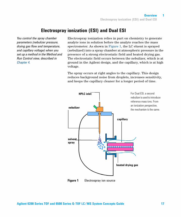
Electrospray ionization relies in part on chemistry to generate analyte ions in solution before the analyte reaches the mass spectrometer. As shown in Figure 1, the LC eluent is sprayed (nebulized) into a spray chamber at atmospheric pressure in the presence of a strong electrostatic field and heated drying gas. The electrostatic field occurs between the nebulizer, which is at ground in the Agilent design, and the capillary, which is at high voltage.
The spray occurs at right angles to the capillary. This design reduces background noise from droplets, increases sensitivity, and keeps the capillary cleaner for a longer period of time.
Figure 1 Electrospray ion source
HPLC inlet
nebulizer
capillary
solventspray
heated drying gas
For Dual ESI, a second
nebulizer is used to introduce
reference mass ions. From
an ionization perspective,
the mechanism is the same.
Agilent 6200 Series TOF and 6500 Series Q-TOF LC/MS System Concepts Guide 17
1 Overview
Electrospray ionization (ESI) and Dual ESI
Electrospray ionization (ESI) consists of four steps:
1 Formation of ions
2 Nebulization
3 Desolvation
4 Ion evaporation
Formation of ions
Ion formation in API-electrospray occurs through more than one mechanism. If the chemistry of analyte, solvents, and buffers is correct, ions are generated in solution before nebulization. This results in high analyte ion concentration and good API-electrospray sensitivity.
Preformed ions are not always required for ESI. Some compounds that do not ionize in solution can still be analyzed. The process of nebulization, desolvation, and ion evaporation creates a strong electrical charge on the surface of the spray droplets. This can induce ionization in analyte molecules at the surface of the droplets.
Nebulization
Nebulization (aerosol generation) takes the sample solution through these steps:
a Sample solution enters the spray chamber through a grounded needle called a nebulizer.
b For high-flow electrospray, nebulizing gas enters the spray chamber concentrically through a tube that surrounds the needle.
c The combination of strong shear forces generated by the nebulizing gas and the strong voltage (2–6 kV) in the spray
18 Agilent 6200 Series TOF and 6500 Series Q-TOF LC/MS System Concepts Guide
Overview 1
Electrospray ionization (ESI) and Dual ESI
chamber draws out the sample solution and breaks it into droplets.
d As the droplets disperse, ions of one polarity preferentially migrate to the droplet surface due to electrostatic forces.
e As a result, the sample is simultaneously charged and dispersed into a fine spray of charged droplets, hence the name electrospray.
Because the sample solution is not heated when the aerosol is created, ESI does not thermally decompose most analytes.
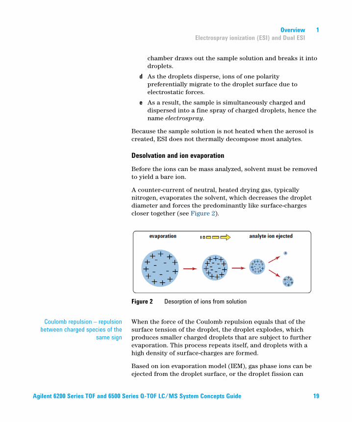
Desolvation and ion evaporation
Before the ions can be mass analyzed, solvent must be removed to yield a bare ion.
A counter-current of neutral, heated drying gas, typically nitrogen, evaporates the solvent, which decreases the droplet diameter and forces the predominantly like surface-charges closer together (see Figure 2).
Coulomb repulsion – repulsion
between charged species of the
same sign
When the force of the Coulomb repulsion equals that of the surface tension of the droplet, the droplet explodes, which produces smaller charged droplets that are subject to further evaporation. This process repeats itself, and droplets with a high density of surface-charges are formed.
Based on ion evaporation model (IEM), gas phase ions can be ejected from the droplet surface, or the droplet fission can
Figure 2 Desorption of ions from solution
Agilent 6200 Series TOF and 6500 Series Q-TOF LC/MS System Concepts Guide 19
1 Overview
Electrospray ionization (ESI) and Dual ESI
continue until gas phase ions are formed based on the charged residue model (CRM). These ions are attracted to and pass through a capillary sampling orifice into the ion optics and mass analyzer.
The importance of solution chemistry
The choice of solvents and buffers is a key to successful ionization with electrospray. Solvents like methanol that have lower heat capacity, surface tension, and dielectric constant, promote nebulization and desolvation. For best results in electrospray mode:
• Adjust solvent pH according to the polarity of ions desired and the pH of the sample.
• To enhance ion desorption, use solvents that have low heats of vaporization and low surface tensions.
• Select solvents that do not neutralize ions through gas-phase reactions such as proton transfer or ion pair reactions.
• To reduce the buildup of salts in the ion source, select more volatile buffers.
Multiple charging
Electrospray is especially useful to analyze large biomolecules such as proteins, peptides, and oligonucleotides, but can also analyze smaller molecules like drugs and environmental contaminants. Large molecules often acquire more than one charge. Because of this multiple charging, you can use electrospray to analyze molecules as large as 150,000 u even though the mass range (or more accurately mass-to-charge ratio) for a typical quadrupole LC/MS instrument is up to 3000 m/z. For example:
100,000 u / 40 z = 2,500 m/z
The optional MassHunter
BioConfirm Software performs the
calculations to accomplish
deconvolution.
When a large molecule acquires many charges, a mathematical process called deconvolution is used to determine the actual molecular weight of the analyte.
20 Agilent 6200 Series TOF and 6500 Series Q-TOF LC/MS System Concepts Guide
Overview 1
Dual Agilent Jet Stream Electrospray Ionization (Dual AJS ESI)
Dual Agilent Jet Stream Electrospray Ionization (Dual AJS ESI)
With the Dual AJS ESI source, the nebulizing gas for the reference spray can be switched for high flow or low flow applications. The second sprayer improves the reference mass stability over a wide range of LC conditions. Low flow applications are typically less than 200 μL/minute. If the flow is approximately 200 μL/minute, either low or high flow may be appropriate.
Both the Dual AJS ESI and the Dual ESI source support two nebulizers for different applications: the standard nebulizer (G1958-60098) and the capillary (or microflow) LC/MS nebulizer (G1946-60260). The main differences are:
• The machined tip of the capillary LC/MS nebulizer has a smaller exit orifice and internal taper.
• The internal diameter (ID) of the internal needle for the capillary LC/MS nebulizer is 50 μm versus 120 μm for the “standard” nebulizer needle.
The recommended flow range (1 to 50 μL/minute) really is capillary flow, whereas flows from 50 to 250 μL/minute are typically described as microflow.
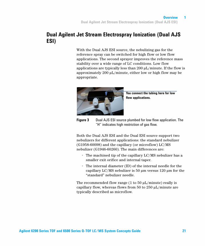
Figure 3 Dual AJS ESI source plumbed for low flow application. The
“H” indicates high restriction of gas flow.
You connect the tubing here for low
flow applications.
Agilent 6200 Series TOF and 6500 Series Q-TOF LC/MS System Concepts Guide 21
1 Overview
Atmospheric pressure chemical ionization (APCI)
Atmospheric pressure chemical ionization (APCI)
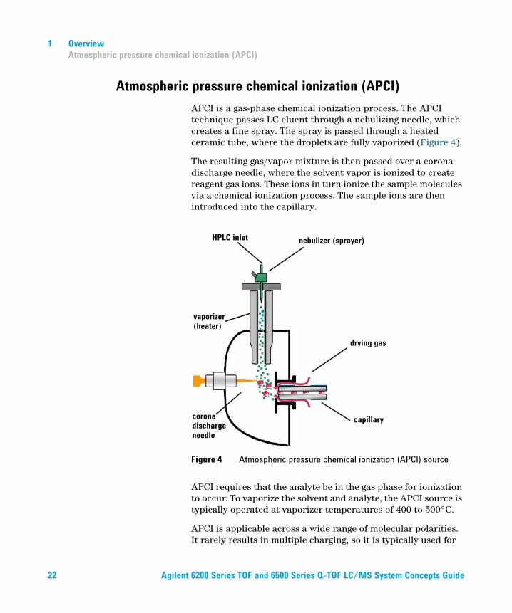
APCI is a gas-phase chemical ionization process. The APCI technique passes LC eluent through a nebulizing needle, which creates a fine spray. The spray is passed through a heated ceramic tube, where the droplets are fully vaporized (Figure 4).
The resulting gas/vapor mixture is then passed over a corona discharge needle, where the solvent vapor is ionized to create reagent gas ions. These ions in turn ionize the sample molecules via a chemical ionization process. The sample ions are then introduced into the capillary.
APCI requires that the analyte be in the gas phase for ionization to occur. To vaporize the solvent and analyte, the APCI source is typically operated at vaporizer temperatures of 400 to 500°C.
APCI is applicable across a wide range of molecular polarities. It rarely results in multiple charging, so it is typically used for
Figure 4 Atmospheric pressure chemical ionization (APCI) source
nebulizer (sprayer)HPLC inlet
vaporizer(heater)
drying gas
capillarycoronadischargeneedle
22 Agilent 6200 Series TOF and 6500 Series Q-TOF LC/MS System Concepts Guide
Overview 1
Atmospheric pressure chemical ionization (APCI)
molecules less than 1,500 u. Because of this molecular weight limitation and use of high-temperature vaporization, APCI is less well-suited than electrospray for analysis of large biomolecules that may be thermally unstable. APCI is well suited for ionization of the less polar compounds that are typically analyzed by normal-phase chromatography.
Agilent 6200 Series TOF and 6500 Series Q-TOF LC/MS System Concepts Guide 23
1 Overview
Atmospheric pressure photoionization (APPI)
Atmospheric pressure photoionization (APPI)
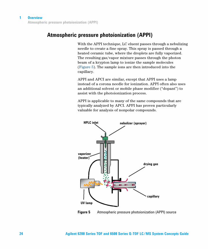
With the APPI technique, LC eluent passes through a nebulizing needle to create a fine spray. This spray is passed through a heated ceramic tube, where the droplets are fully vaporized. The resulting gas/vapor mixture passes through the photon beam of a krypton lamp to ionize the sample molecules (Figure 5). The sample ions are then introduced into the capillary.
APPI and APCI are similar, except that APPI uses a lamp instead of a corona needle for ionization. APPI often also uses an additional solvent or mobile phase modifier (“dopant”) to assist with the photoionization process.
APPI is applicable to many of the same compounds that are typically analyzed by APCI. APPI has proven particularly valuable for analysis of nonpolar compounds.
Figure 5 Atmospheric pressure photoionization (APPI) source
HPLC inlet nebulizer (sprayer)
drying gas
capillary
vaporizer(heater)
UV lamp
24 Agilent 6200 Series TOF and 6500 Series Q-TOF LC/MS System Concepts Guide
Overview 1
Multimode ionization (MMI)
Multimode ionization (MMI)
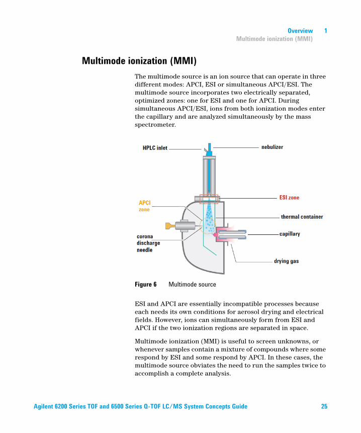
The multimode source is an ion source that can operate in three different modes: APCI, ESI or simultaneous APCI/ESI. The multimode source incorporates two electrically separated, optimized zones: one for ESI and one for APCI. During simultaneous APCI/ESI, ions from both ionization modes enter the capillary and are analyzed simultaneously by the mass spectrometer.
ESI and APCI are essentially incompatible processes because each needs its own conditions for aerosol drying and electrical fields. However, ions can simultaneously form from ESI and APCI if the two ionization regions are separated in space.
Multimode ionization (MMI) is useful to screen unknowns, or whenever samples contain a mixture of compounds where some respond by ESI and some respond by APCI. In these cases, the multimode source obviates the need to run the samples twice to accomplish a complete analysis.
Figure 6 Multimode source
Agilent 6200 Series TOF and 6500 Series Q-TOF LC/MS System Concepts Guide 25
1 Overview
Multimode ionization (MMI)
Unlike the APCI and APPI, with the multimode source, the actual vapor temperature, and not the vaporizer temperature, is monitored. As a result, the vaporizer is typically set to between 200°C and 250°C.
26 Agilent 6200 Series TOF and 6500 Series Q-TOF LC/MS System Concepts Guide
Overview 1
How does the Agilent TOF and Q-TOF mass spectrometer work?
How does the Agilent TOF and Q-TOF mass spectrometer work?
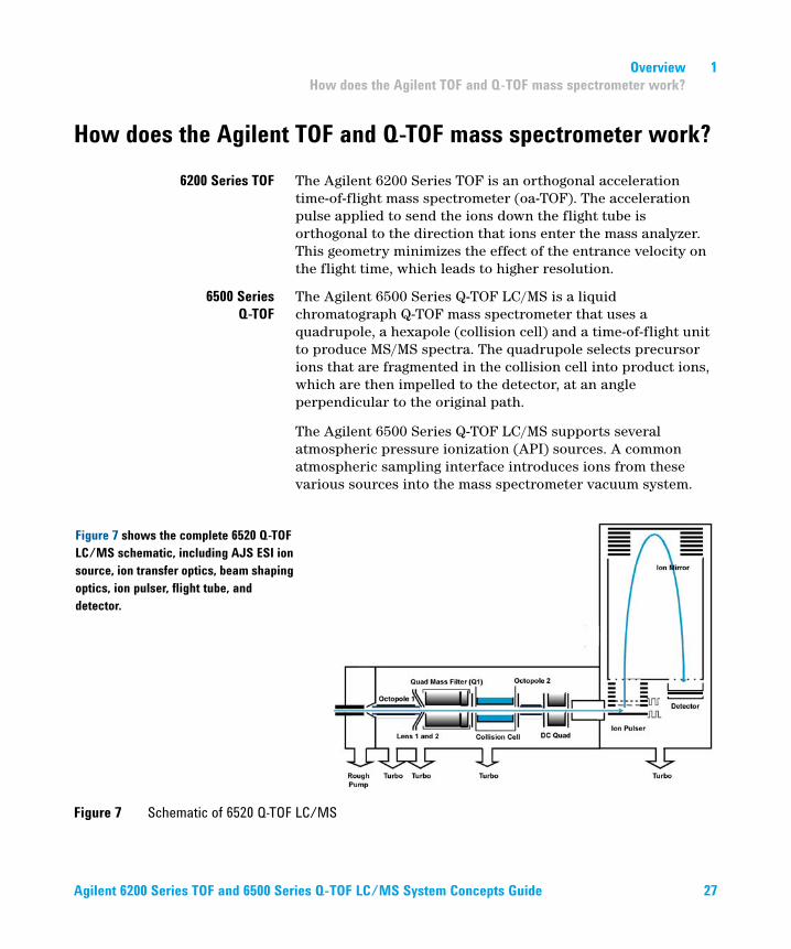
6200 Series TOF The Agilent 6200 Series TOF is an orthogonal acceleration time-of-flight mass spectrometer (oa-TOF). The acceleration pulse applied to send the ions down the flight tube is orthogonal to the direction that ions enter the mass analyzer. This geometry minimizes the effect of the entrance velocity on the flight time, which leads to higher resolution.
6500 Series
Q-TOF
The Agilent 6500 Series Q-TOF LC/MS is a liquid chromatograph Q-TOF mass spectrometer that uses a quadrupole, a hexapole (collision cell) and a time-of-flight unit to produce MS/MS spectra. The quadrupole selects precursor ions that are fragmented in the collision cell into product ions, which are then impelled to the detector, at an angle perpendicular to the original path.
The Agilent 6500 Series Q-TOF LC/MS supports several atmospheric pressure ionization (API) sources. A common atmospheric sampling interface introduces ions from these various sources into the mass spectrometer vacuum system.
Figure 7 Schematic of 6520 Q-TOF LC/MS
Figure 7 shows the complete 6520 Q-TOF
LC/MS schematic, including AJS ESI ion
source, ion transfer optics, beam shaping
optics, ion pulser, flight tube, and
detector.
Agilent 6200 Series TOF and 6500 Series Q-TOF LC/MS System Concepts Guide 27
1 Overview
How does the Agilent TOF and Q-TOF mass spectrometer work?
d
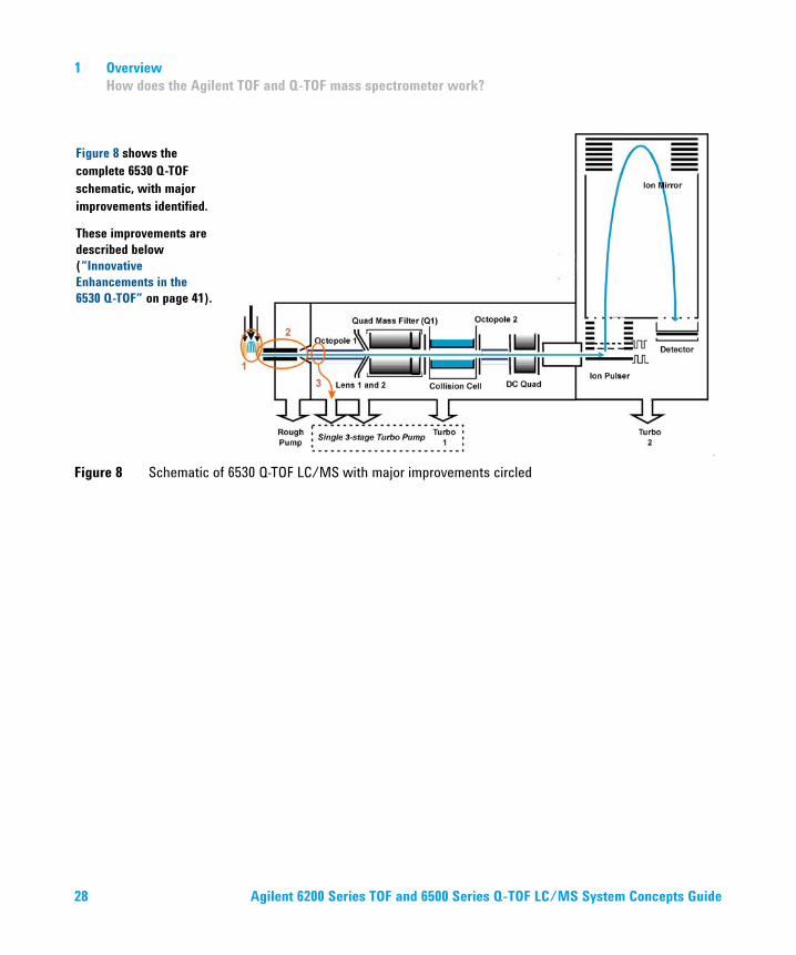
Figure 8 Schematic of 6530 Q-TOF LC/MS with major improvements circled
Figure 8 shows the
complete 6530 Q-TOF
schematic, with major
improvements identified.
These improvements are
described below
(“Innovative
Enhancements in the
6530 Q-TOF” on page 41).
28 Agilent 6200 Series TOF and 6500 Series Q-TOF LC/MS System Concepts Guide
Overview 1
How does the Agilent TOF and Q-TOF mass spectrometer work?
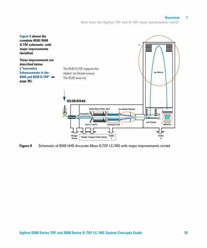
Figure 9 Schematic of 6540 UHD Accurate-Mass Q-TOF LC/MS with major improvements circled
Figure 9 shows the
complete 6538/6540
Q-TOF schematic, with
major improvements
identified.
These improvements are
described below
(“Innovative
Enhancements in the
6540 and 6538 Q-TOF” on
page 39).
The 6540 Q-TOF supports the
Agilent Jet Stream source.
The 6538 does not.
Agilent 6200 Series TOF and 6500 Series Q-TOF LC/MS System Concepts Guide 29
1 Overview
How does the Agilent TOF and Q-TOF mass spectrometer work?
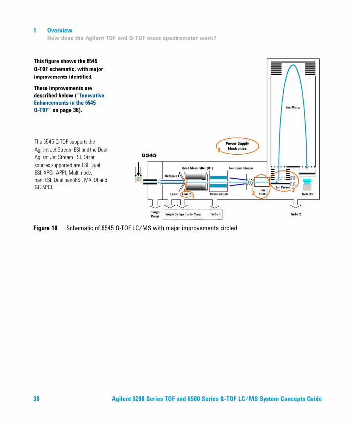
Figure 10 Schematic of 6545 Q-TOF LC/MS with major improvements circled
This figure shows the 6545
Q-TOF schematic, with major
improvements identified.
These improvements are
described below (“Innovative
Enhancements in the 6545
Q-TOF” on page 38).
The 6545 Q-TOF supports the
Agilent Jet Stream ESI and the Dual
Agilent Jet Stream ESI. Other
sources supported are ESI, Dual
ESI, APCI, APPI, Multimode,
nanoESI, Dual nanoESI, MALDI and
GC-APCI.
30 Agilent 6200 Series TOF and 6500 Series Q-TOF LC/MS System Concepts Guide
Overview 1
How does the Agilent TOF and Q-TOF mass spectrometer work?
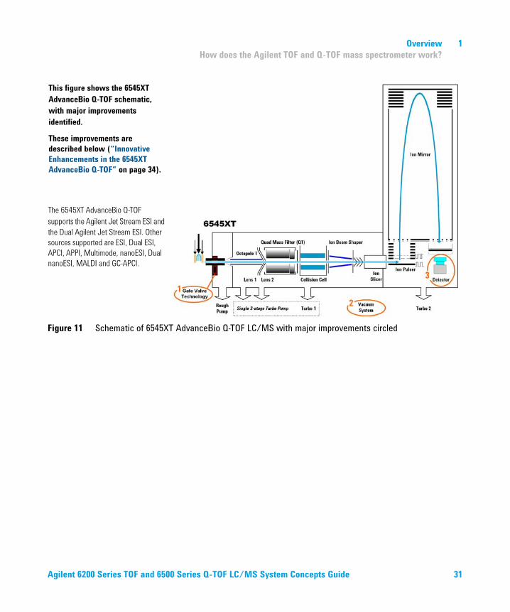
Figure 11 Schematic of 6545XT AdvanceBio Q-TOF LC/MS with major improvements circled
This figure shows the 6545XT
AdvanceBio Q-TOF schematic,
with major improvements
identified.
These improvements are
described below (“Innovative
Enhancements in the 6545XT
AdvanceBio Q-TOF” on page 34).
The 6545XT AdvanceBio Q-TOF
supports the Agilent Jet Stream ESI and
the Dual Agilent Jet Stream ESI. Other
sources supported are ESI, Dual ESI,
APCI, APPI, Multimode, nanoESI, Dual
nanoESI, MALDI and GC-APCI.
Agilent 6200 Series TOF and 6500 Series Q-TOF LC/MS System Concepts Guide 31
1 Overview
How does the Agilent TOF and Q-TOF mass spectrometer work?
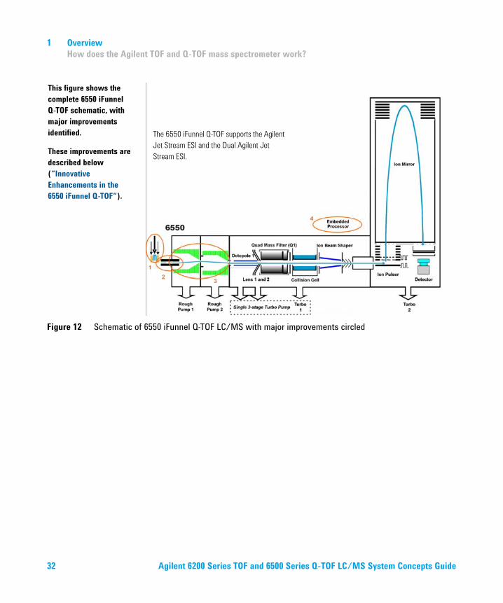
Figure 12 Schematic of 6550 iFunnel Q-TOF LC/MS with major improvements circled
This figure shows the
complete 6550 iFunnel
Q-TOF schematic, with
major improvements
identified.
These improvements are
described below
(“Innovative
Enhancements in the
6550 iFunnel Q-TOF”).
The 6550 iFunnel Q-TOF supports the Agilent
Jet Stream ESI and the Dual Agilent Jet
Stream ESI.
32 Agilent 6200 Series TOF and 6500 Series Q-TOF LC/MS System Concepts Guide
Overview 1
How does the Agilent TOF and Q-TOF mass spectrometer work?
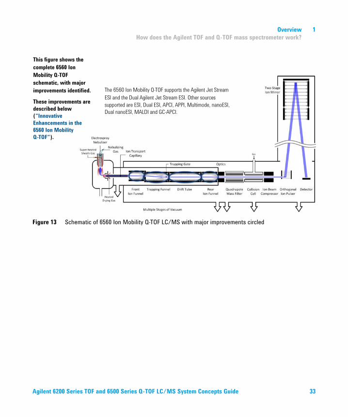
Figure 13 Schematic of 6560 Ion Mobility Q-TOF LC/MS with major improvements circled
This figure shows the
complete 6560 Ion
Mobility Q-TOF
schematic, with major
improvements identified.
These improvements are
described below
(“Innovative
Enhancements in the
6560 Ion Mobility
Q-TOF”).
The 6560 Ion Mobility Q-TOF supports the Agilent Jet Stream
ESI and the Dual Agilent Jet Stream ESI. Other sources
supported are ESI, Dual ESI, APCI, APPI, Multimode, nanoESI,
Dual nanoESI, MALDI and GC-APCI.
Agilent 6200 Series TOF and 6500 Series Q-TOF LC/MS System Concepts Guide 33
1 Overview
Innovative Enhancements in the 6545XT AdvanceBio Q-TOF
Innovative Enhancements in the 6545XT AdvanceBio Q-TOF
See Figure 11 on page 31 for a schematic of the 6545XT AdvanceBio Q-TOF.
Gate Valve
The 6545XT has Gate Valve Technology which enables higher uptime and increased productivity by allowing capillary replacement without having to vent the instrument. A Capillary Puller tool is included to allow you to pull the capillary from the desolvation chamber without venting the system. The safety lock is designed to prevent the Gate Valve from being accidentally opened or closed.
Vacuum System
The MS40+ with oil-isolation valve protection prevents suck-back in case of a sudden power outage or unexpected vent. It also improves the oil pump long term reliability.
The turbo vacuum speed is improved, and the system has an additional differential pumping vacuum zone.
Detector Mounting
The detector now has a kinematic mount which keeps the detector in the optimum position for detection of every transient.
TOF Manifold bakeout heater
A TOF manifold heater and fan are available. You use the Bakeout tool in the Diagnostics program to improve the vacuum more quickly. If you do not perform a low temperature bakeout after exposure to atmosphere, your vacuum pressure may take longer to achieve good operating conditions for enhanced mass accuracy for multiply charged molecules or intact species. You start the Heater Control tool from the Q-TOF Diagnostics Tool.
34 Agilent 6200 Series TOF and 6500 Series Q-TOF LC/MS System Concepts Guide
Overview 1
Innovative Enhancements in the 6560 Ion Mobility Q-TOF
Innovative Enhancements in the 6560 Ion Mobility Q-TOF
Front funnel
Ions generated in the source region are carried into the front funnel through a single bore capillary. The front funnel improves the sensitivity by efficiently transferring gas phase ions into the trapping funnel while it pumps away excess gas and neutral molecules. The front funnel operates at high pressure.
Trapping funnel
The trapping funnel accumulates and releases ions into the drift tube. The continuous ion beam from the electrospray process has to be converted into a pulsed ion beam prior to ion mobility separation. The trapping funnel first stores and then releases discrete packets of ions into the drift tube.
Also, a tapered section at the exit region of the trapping funnel is designed to focus the ion packets into the drift cell to avoid ion losses and improve resolution and sensitivity. High abundance, well-confined packet of ions enter the drift tube, which results in high drift resolution and high sensitivity.
Drift tube
The drift cell is approximately 80 cm long and generally operated at 20 V/cm or less drift field. Ions are separated as they pass through the drift tube based on their collision cross section and charge. Ions with larger collision cross sections undergo a higher number of collisions with drift gas molecules compared to ions with smaller collision cross section. Therefore, larger ions travel through the drift tube slower than the smaller ions. Also, ions with higher charge states experience a higher electric force, and hence travel at a higher velocity, compared to ions with lower charge states. The drift tube is operated under low field limit conditions that allow the instrument to generate accurate structural information for compounds. Under the low electric field conditions the mobility is not dependent on the electric field but rather on the structure
Agilent 6200 Series TOF and 6500 Series Q-TOF LC/MS System Concepts Guide 35
1 Overview
Innovative Enhancements in the 6550 iFunnel Q-TOF
of the molecule and its interaction with the buffer gas. In addition to separating ions based on their structures, experiments can be performed to quantify this collision cross section value.
Rear funnel
Ions that leave the drift tube enter the rear funnel, which efficiently refocuses and transfers ions to the mass analyzer through a hexapole ion guide.
Innovative Enhancements in the 6550 iFunnel Q-TOF
See Figure 12 on page 32 for a schematic of the 6550 Q-TOF.
Dual Agilent Jet Stream Electrospray
The Dual Agilent Jet Stream Electrospray source allows you to modify it for high flow and low flow applications. See “Dual Agilent Jet Stream Electrospray Ionization (Dual AJS ESI)” on page 21 for more information.
iFunnel Technology
The iFunnel Technology encompasses two enhancements to the 6550 iFunnel Q-TOF: the Agilent Jet Stream source, a hexabore capillary and the Dual Ion Funnel technology.
36 Agilent 6200 Series TOF and 6500 Series Q-TOF LC/MS System Concepts Guide
Overview 1
Innovative Enhancements in the 6550 iFunnel Q-TOF
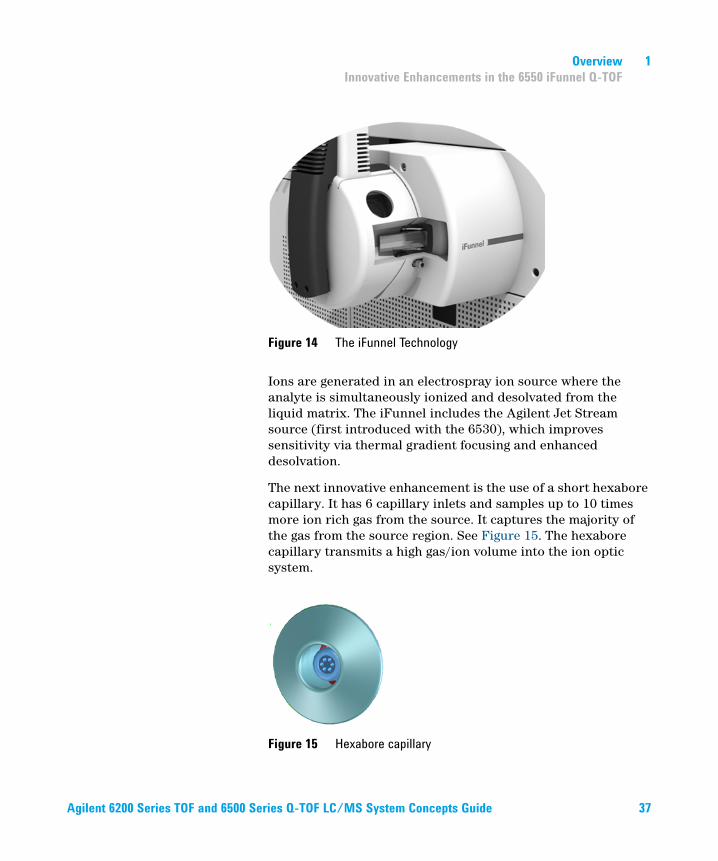
Ions are generated in an electrospray ion source where the analyte is simultaneously ionized and desolvated from the liquid matrix. The iFunnel includes the Agilent Jet Stream source (first introduced with the 6530), which improves sensitivity via thermal gradient focusing and enhanced desolvation.
The next innovative enhancement is the use of a short hexabore capillary. It has 6 capillary inlets and samples up to 10 times more ion rich gas from the source. It captures the majority of the gas from the source region. See Figure 15. The hexabore capillary transmits a high gas/ion volume into the ion optic system.
Figure 14 The iFunnel Technology
Figure 15 Hexabore capillary
Agilent 6200 Series TOF and 6500 Series Q-TOF LC/MS System Concepts Guide 37
1 Overview
Innovative Enhancements in the 6545 Q-TOF
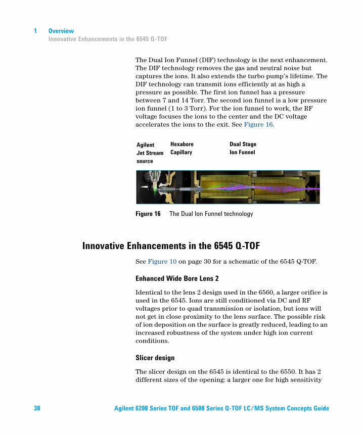
The Dual Ion Funnel (DIF) technology is the next enhancement. The DIF technology removes the gas and neutral noise but captures the ions. It also extends the turbo pump’s lifetime. The DIF technology can transmit ions efficiently at as high a pressure as possible. The first ion funnel has a pressure between 7 and 14 Torr. The second ion funnel is a low pressure ion funnel (1 to 3 Torr). For the ion funnel to work, the RF voltage focuses the ions to the center and the DC voltage accelerates the ions to the exit. See Figure 16.
Innovative Enhancements in the 6545 Q-TOF
See Figure 10 on page 30 for a schematic of the 6545 Q-TOF.
Enhanced Wide Bore Lens 2
Identical to the lens 2 design used in the 6560, a larger orifice is used in the 6545. Ions are still conditioned via DC and RF voltages prior to quad transmission or isolation, but ions will not get in close proximity to the lens surface. The possible risk of ion deposition on the surface is greatly reduced, leading to an increased robustness of the system under high ion current conditions.
Slicer design
The slicer design on the 6545 is identical to the 6550. It has 2 different sizes of the opening: a larger one for high sensitivity
Figure 16 The Dual Ion Funnel technology
Agilent
Jet Stream
source
Hexabore
Capillary
Dual Stage
Ion Funnel
38 Agilent 6200 Series TOF and 6500 Series Q-TOF LC/MS System Concepts Guide
Overview 1
Innovative Enhancements in the 6540 and 6538 Q-TOF
applications, and a smaller one for high resolution applications. The positions can be changed in the Tune Context and are saved as part of the tune file. In total, 10 positions are usable: 4 positions for the high sensitivity, and 6 positions for high resolution.
Improved pulser design
Thermal and longterm stability of the pulser is optimized by better process control of the delay time, leading to less variations in mass accuracy.
Improved Power Supplies
In comparison to the 6540, changes were made to the feed-through as well as the type of power supply for better thermal and other environmental stability. As a consequence, better resolution is achieved with this change.
Dual Agilent Jet Stream Electrospray
The Dual Agilent Jet Stream Electrospray source allows you to modify it for high flow and low flow applications. See “Dual Agilent Jet Stream Electrospray Ionization (Dual AJS ESI)” on page 21 for more information.
Innovative Enhancements in the 6540 and 6538 Q-TOF
See Figure 9 on page 29 for a schematic of the 6540 Q-TOF.
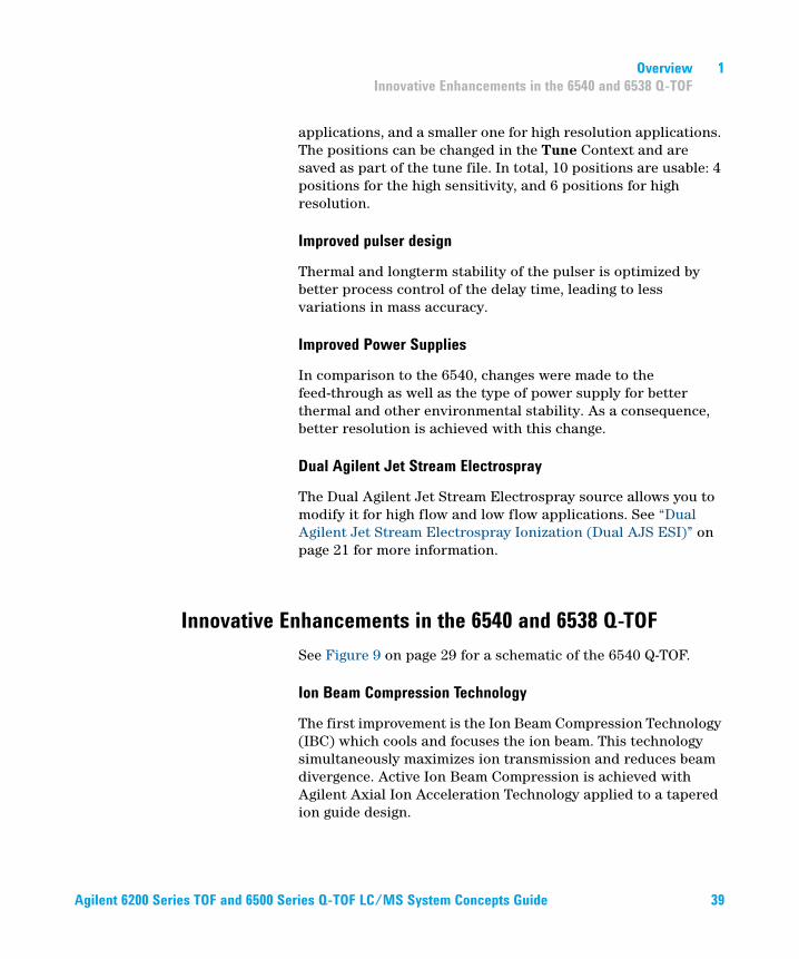
Ion Beam Compression Technology
The first improvement is the Ion Beam Compression Technology (IBC) which cools and focuses the ion beam. This technology simultaneously maximizes ion transmission and reduces beam divergence. Active Ion Beam Compression is achieved with Agilent Axial Ion Acceleration Technology applied to a tapered ion guide design.
Agilent 6200 Series TOF and 6500 Series Q-TOF LC/MS System Concepts Guide 39
1 Overview
Innovative Enhancements in the 6540 and 6538 Q-TOF
Ion beam compression provides up to a 10-fold compression and cooling which helps in creating a much denser and thinner ion beam that passes through a narrower slit leading into the slicer and pulser region. The narrowed, cooled and condensed beam is a key factor in enabling the gain in mass resolution to 40,000 while maintaining excellent sensitivity.
Extended Flight Tube with Enhanced Mirror Technology (EMT)
The second improvement is that the flight tube for the 6538/6540 Q-TOF is now five feet long.
The 1 ppm/C Expansion Coefficient for the Inner Flight Tube virtually eliminates calibration drift due to flight tube elongation. The second order temporal focusing ion mirror uses a high transmission Harp Grid for maximum sensitivity.
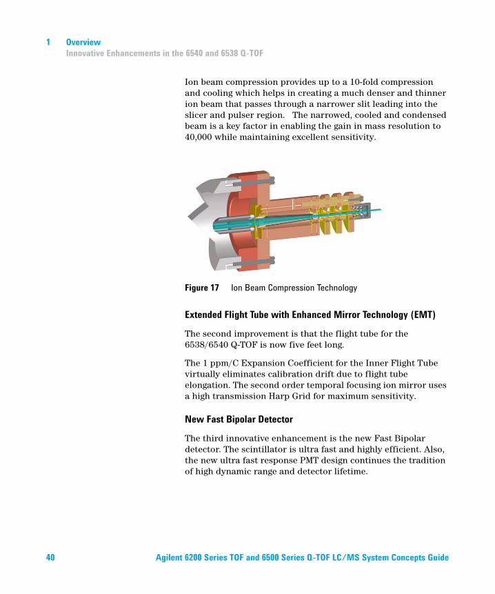
New Fast Bipolar Detector
The third innovative enhancement is the new Fast Bipolar detector. The scintillator is ultra fast and highly efficient. Also, the new ultra fast response PMT design continues the tradition of high dynamic range and detector lifetime.
Figure 17 Ion Beam Compression Technology
40 Agilent 6200 Series TOF and 6500 Series Q-TOF LC/MS System Concepts Guide
Overview 1
Innovative Enhancements in the 6530 Q-TOF
Innovative Enhancements in the 6530 Q-TOF
See Figure 8 on page 28 for a schematic of the 6530 Q-TOF.
Ions are generated using an electrospray ion source where the analyte is simultaneously ionized and desolvated from the liquid matrix. The first of three (3) innovative Agilent enhancements is found in the Agilent Jet Stream source (denoted as 1 in Figure 8) which improves sensitivity via thermal gradient focusing and enhanced desolvation. This source is described in detail below (“Agilent Jet Stream Thermal Gradient Source” on page 42).
The desolvated ions then enter the mass spectrometer via an innovative resistive and highly inert capillary transfer tube (denoted as 2 in Figure 8) that improves ion transmission and allows virtually instantaneous polarity switching.
Further increase in ion transmission is obtained by improvement of the pumping speed in vacuum stage 2, resulting in better ion capture by the first octopole (denoted as 3 in Figure 8). The ions next pass through the optics and into the quadrupole analyzer. The quadrupole analyzer consists of four parallel hyperbolic rods through which selected ions based on their mass to charge ratio are filtered.
Figure 18 Fast Bipolar Detector
Agilent 6200 Series TOF and 6500 Series Q-TOF LC/MS System Concepts Guide 41
1 Overview
Agilent Jet Stream Thermal Gradient Source
The ions passing through the quadrupole analyzer are then directed through the collision cell where they are fragmented. The collision cell is actually a hexapole filled with nitrogen, the same gas that is used as the drying gas. The collision cell design has axial acceleration for high speed MS/MS analysis. Fragment ions formed in the collision cell are then sent to the TOF to enable a user to isolate and examine product ions with respect to precursor ions.
Agilent Jet Stream Thermal Gradient Source
This source is supported on the 6530, 6540, 6550, and the 6230 LC/MS instruments.
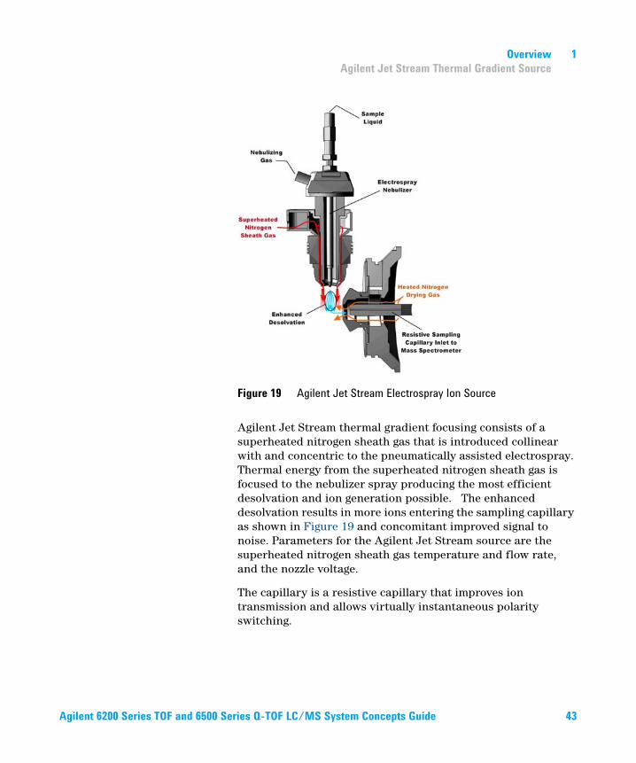
Agilent Jet Stream source enhances analyte desolvation by collimating the nebulizer spray and creating a dramatically “brighter signal.” The addition of a collinear, concentric, super-heated nitrogen sheath gas (Figure 19) to the inlet assembly significantly improves ion drying from the electrospray plume and leads to increased mass spectrometer signal to noise. The 6530 Q-TOF gets attomole-to-low-femtomole sensitivity for superior trace level analyses.
42 Agilent 6200 Series TOF and 6500 Series Q-TOF LC/MS System Concepts Guide
Overview 1
Agilent Jet Stream Thermal Gradient Source
Agilent Jet Stream thermal gradient focusing consists of a superheated nitrogen sheath gas that is introduced collinear with and concentric to the pneumatically assisted electrospray. Thermal energy from the superheated nitrogen sheath gas is focused to the nebulizer spray producing the most efficient desolvation and ion generation possible. The enhanced desolvation results in more ions entering the sampling capillary as shown in Figure 19 and concomitant improved signal to noise. Parameters for the Agilent Jet Stream source are the superheated nitrogen sheath gas temperature and flow rate, and the nozzle voltage.
The capillary is a resistive capillary that improves ion transmission and allows virtually instantaneous polarity switching.
Figure 19 Agilent Jet Stream Electrospray Ion Source
Agilent 6200 Series TOF and 6500 Series Q-TOF LC/MS System Concepts Guide 43
1 Overview
Front-end ion optics
Front-end ion optics
For information on the various ion sources, see “How do different ion sources work?” on page 16
After the API source forms ions, the 6200 Series TOF or 6500 Series Q-TOF LC/MS system performs the following operations, organized according to the stages of the ion path and the vacuum stages of the TOF or Q-TOF. See Figure 7 on page 27 for details.
Ion enrichment (Vacuum stage 1)
Ions produced in an API source are electrostatically drawn through a drying gas and then pneumatically conducted through a heated sampling capillary into the first stage of the vacuum system. The majority of drying gas and solvent vapor are deflected by the skimmer and exhausted by a rough pump. The ions that pass through the skimmer pass into the second stage of the vacuum system.
Ion transport 1 (Vacuum stage 2 and vacuum stage 3)
An octopole ion guide is a set of
small parallel metal rods with a
common open axis through which
the ions can pass.
In this stage the ions are immediately focused by an octopole ion guide. Radio frequency voltage applied to the parallel octopole rods repel ions above a particular mass range toward the center of the rod set. The ions pass through the octopole ion guide because of the momentum obtained from being drawn from atmospheric pressure through the sampling capillary.
In a Q-TOF and in the 6224 and 6230 TOF, the octopole spans both the 2nd and the 3rd vacuum stages. Ions exit the octopole and pass through two focusing lenses and an RF lens.
In an 6220 TOF, the ions exit the first ion guide and pass into the third stage of the vacuum system. In the third stage of the vacuum, the ions are passed onto a second octopole assembly (octopole 2) which then sends the ion on to the beam shaping assembly.
44 Agilent 6200 Series TOF and 6500 Series Q-TOF LC/MS System Concepts Guide
Overview 1
Front-end ion optics
Ion transport 2 (Vacuum stage 4 for 6220 TOF only)
In this fourth vacuum pumping stage, the pressure is now low enough that collisions of the ions with gas molecules occur less frequently.
Ion selection (Vacuum stage 4 for Q-TOF only)
Lens 2 RF The phase of lens 2 RF is matched to that of the subsequent quadrupole resulting in a significantly increased sensitivity. Dynamic lens 2 DC and RF values are additionally used to further increase m/z dependent transmission upon isolation.
Quad mass
filters
The quadrupoles consist of hyperbolic rods that optimize ion transmission and spectral resolution. There tends to be more ion loss with circular rods.
Pre-filter The end section of the quadrupole also consists of short hyperbolic rods, but their RF voltages are only high enough to guide ions into the collision cell.
Ion fragmentation 2 (Vacuum stage 4 for Q-TOF only)
Ions selected by the quadrupole are then passed to the collision cell where they are fragmented.
The axial acceleration collision cell is a high pressure hexapole assembly with its axial acceleration adjusted to maximize sensitivity while eliminating crosstalk.
Crosstalk occurs when product ions from a previously selected precursor appear in a product ion spectrum of a subsequently selected precursor because of slow clearance from the collision cell. This creates a composite product ion spectrum which can be difficult to interpret.
NOTEThe following sections are only part of the Q-TOF LC/MS instrument. The
next section in the TOF instrument is the Beam shaping (Vacuum stage 3
for TOF and 4 for Q-TOF) on page 47.
Agilent 6200 Series TOF and 6500 Series Q-TOF LC/MS System Concepts Guide 45
1 Overview
Front-end ion optics
The components that contribute to this higher sensitivity and faster response are
• Small diameter hexapole collision cell
• High frequency hexapole collision cell
• Linear axial acceleration
• High pressure collision cell
• High speed digital electronics
The collision cell contains nitrogen, the same gas that is used in the ion source. The small diameter of the hexapole assembly assists in capturing fragmented ions.
Why a hexapole? The geometry of a hexapole provides advantages in two domains: ion focusing and ion transmission.
• The first advantage is in ion focusing where a quadrupole is better than a hexapole, which is better than an octopole, that is, quadrupole > hexapole > octopole.
• The second advantage involves ion transmission across a wide mass range, or m/z bandwidth. In this case, the octopole is better than the hexapole, which is better than the quadrupole.
The hexapole is chosen because overall, it is the best for both ion focusing and ion transmission.
Collision cell design The collision cell hexapole consists of six resistively coated rods used to generate a potential difference across the length of the collision cell.
A potential difference is always present. This ensures that the precursor ions coming from the quadrupole or fragment ions generated in the collision cell are transmitted and not allowed to drift around at random.
Sweeping out the ions in this manner avoids the issue of crosstalk where residual product ions from a previous experiment can interfere with the product ion spectrum of a subsequent experiment. A collision energy voltage is applied over the accelerating linear voltage to generate fragments or product ions.
46 Agilent 6200 Series TOF and 6500 Series Q-TOF LC/MS System Concepts Guide
Overview 1
Front-end ion optics
Beam shaping (Vacuum stage 3 for TOF and 4 for Q-TOF)
To facilitate beam shaping, lenses focus the ions so that they enter the time-of-flight analyzer as a parallel beam. The more parallel the ion beam, the higher the resolution in the resulting mass spectrum. After the ions have been shaped into a parallel beam, they pass through a slit opening into the last vacuum stage where the time-of-flight analysis takes place.
In the 6540, 6550, and 6560 LC/MS, ions enter the ion beam compressor. Ion beam compression provides up to a 10-fold compression and cooling which helps in creating a much denser and thinner ion beam that passes through a narrower slit leading into the slicer and pulser region.
Flight tube/Mass Analyzer (Vacuum stage 4 for 6224/6230 TOF) (Vacuum stage 5 for 6500 Series Q-TOF)
Ion pulser The nearly parallel beam of ions passes into the time-of-flight ion pulser. The ion pulser is a stack of plates, each one (except the back plate) with a center hole. The ions pass into this stack from the side just between the back plate and the first plate with its center hole. To start the flight of the ions to the detector, a high voltage (HV) pulse is applied to the back plate. The applied pulse accelerates the ions through the stack of pulser plates, acting as a rapid-fire ion gun.
Flight tube The ions leave the ion pulser and travel through the flight tube (see Figure 7). At the opposite end of the flight tube is an ion “mirror”, which reflects the ions that arrive near the end of the flight tube towards the ion pulser. Because the ions entered the ion pulser with a certain amount of forward momentum orthogonal to the flight direction in the flight tube, they never return to the ion pulser, but move to where the ion detector is mounted.
The ion mirror increases the resolving power of the instrument by effectively doubling the flight distance (from one meter to two meters) in the same space, and by performing a refocusing operation so that ions having different initial velocities still arrive simultaneously at the detector.
Agilent 6200 Series TOF and 6500 Series Q-TOF LC/MS System Concepts Guide 47
This page intentionally left blank.
Because the calculation for the mass of each ion depends on its flight time in the flight tube, the background gas pressure must be very low. Any collision of an ion with residual gas slows the ion on its path to the detector and affects the accuracy of the mass calculation.
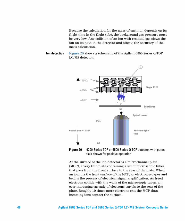
Ion detection Figure 20 shows a schematic of the Agilent 6500 Series Q-TOF LC/MS detector.
Figure 20 6200 Series TOF or 6500 Series Q-TOF detector, with poten-
tials shown for positive operation
At the surface of the ion detector is a microchannel plate (MCP), a very thin plate containing a set of microscopic tubes that pass from the front surface to the rear of the plate. When an ion hits the front surface of the MCP, an electron escapes and begins the process of electrical signal amplification. As freed electrons collide with the walls of the microscopic tubes, an ever-increasing cascade of electrons travels to the rear of the plate. Roughly 10 times more electrons exit the MCP than incoming ions contact the surface.
48 Agilent 6200 Series TOF and 6500 Series Q-TOF LC/MS System Concepts Guide
Overview 1
Front-end ion optics
These electrons are then focused onto a scintillator, which, when struck by electrons, produces a flash of light. The light from the scintillator is focused through two small lenses onto a photomultiplier tube (PMT), which produces the electrical signal read by the data system. The reason for producing an optical signal from the MCP electrons is because the output of the MCP is at roughly -6000 volts. The light produced by the scintillator passes to the PMT, which has a signal output at ground potential.
Agilent 6200 Series TOF and 6500 Series Q-TOF LC/MS System Concepts Guide 49

50 Agilent 6200 Series TOF and 6500 Series Q-TOF LC/MS System Concepts Guide
This page intentionally left blank.
Agilent 6200 Series TOF and 6500 Series Q-TOF LC/MS System
2Instrument Preparation
LC preparation 52
LC module setup 52
Column equilibration and conditioning 55
TOF and Q-TOF preparation – calibration and tuning 57
TOF mass calibration 58
Tuning choices 60
Tune reports 71
Storage and retrieval of tune results and Instrument Mode 72
Tune Set Point Modifications for Medium and Large Proteins 74
Real-time displays 75
Instrument Status Window 75
Real-time parameter values (Actuals) 76
Real-time Chromatogram Plot and Spectral Plot windows 78
System logbook 80
Learn about the concepts that can help you prepare the instrument for use.
This chapter assumes that the hardware and software are installed, the instrument is configured and the performance verified. If this has not been completed, see the Agilent 6200 Series Time-of-Flight LC/MS System Installation Guide or the Agilent 6500 Series Quadrupole Time-of-Flight LC/MS System Installation Guide.
51
2 Instrument Preparation
LC preparation
LC preparation
To install, configure and start the
LC modules, see the Installation
Guide.
To prepare the LC for sample runs, you usually do three tasks:
• Set up the LC modules for operation
• Equilibrate or condition the column
• Monitor the plot baseline to assure pump and column stability (See “Real-time displays” on page 75.)
See the Quick Start Guide and
online Help for instructions on how
to prepare the LC for a sample run.
You can also view the system logbook for explanations of errors. (See “System logbook” on page 80.)
LC module setup
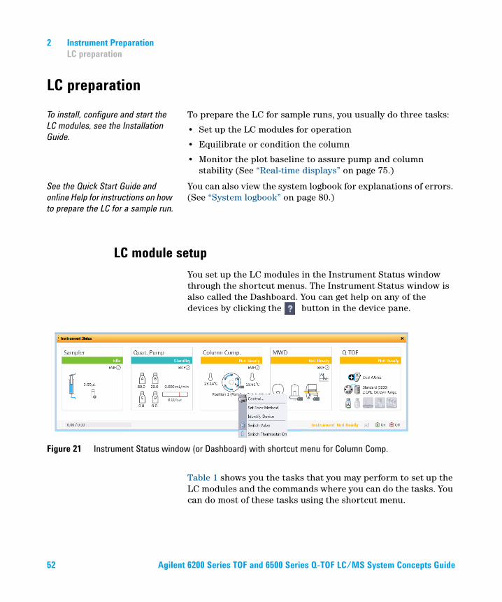
You set up the LC modules in the Instrument Status window through the shortcut menus. The Instrument Status window is also called the Dashboard. You can get help on any of the devices by clicking the button in the device pane.
Table 1 shows you the tasks that you may perform to set up the LC modules and the commands where you can do the tasks. You can do most of these tasks using the shortcut menu.
Figure 21 Instrument Status window (or Dashboard) with shortcut menu for Column Comp.
52 Agilent 6200 Series TOF and 6500 Series Q-TOF LC/MS System Concepts Guide
Instrument Preparation 2
LC module setup
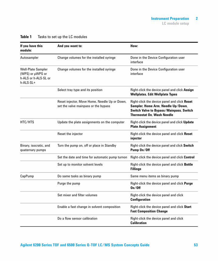
Table 1 Tasks to set up the LC modules
If you have this
module:
And you want to: How:
Autosampler Change volumes for the installed syringe Done in the Device Configuration user
interface
Well-Plate Sampler
(WPS) or µWPS or
h-ALS or h-ALS-SL or
h-ALS-SL+
Change volumes for the installed syringe Done in the Device Configuration user
interface
Select tray type and its position Right-click the device panel and click Assign
Wellplates, Edit Wellplate Types
Reset injector, Move Home, Needle Up or Down,
set the valve mainpass or the bypass
Right-click the device panel and click Reset
Sampler, Home Arm, Needle Up/Down,
Switch Valve to Bypass/Mainpass, Switch
Thermostat On, Wash Needle
HTC/HTS Update the plate assignments on the computer Right-click the device panel and click Update
Plate Assignment
Reset the injector Right-click the device panel and click Reset
injector
Binary, isocratic, and
quaternary pumps
Turn the pump on, off or place in Standby Right-click the device panel and click Switch
Pump On/Off
Set the date and time for automatic pump turnon Right-click the device panel and click Control
Set up to monitor solvent levels Right-click the device panel and click Bottle
Fillings
CapPump Do same tasks as binary pump Same menu items as binary pump
Purge the pump Right-click the device panel and click Purge
On/Off
Set mixer and filter volumes Right-click the device panel and click
Configuration
Enable a fast change in solvent composition Right-click the device panel and click Start
Fast Composition Change
Do a flow sensor calibration Right-click the device panel and click
Calibration
Agilent 6200 Series TOF and 6500 Series Q-TOF LC/MS System Concepts Guide 53
2 Instrument Preparation
LC module setup
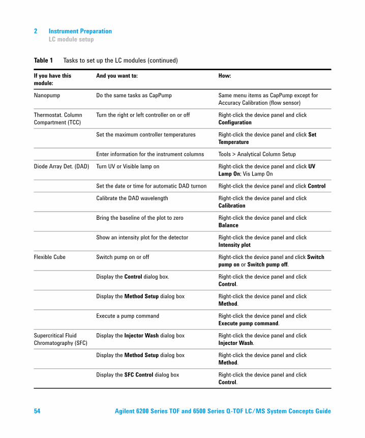
Nanopump Do the same tasks as CapPump Same menu items as CapPump except for
Accuracy Calibration (flow sensor)
Thermostat. Column
Compartment (TCC)
Turn the right or left controller on or off Right-click the device panel and click
Configuration
Set the maximum controller temperatures Right-click the device panel and click Set
Temperature
Enter information for the instrument columns Tools > Analytical Column Setup
Diode Array Det. (DAD) Turn UV or Visible lamp on Right-click the device panel and click UV
Lamp On; Vis Lamp On
Set the date or time for automatic DAD turnon Right-click the device panel and click Control
Calibrate the DAD wavelength Right-click the device panel and click
Calibration
Bring the baseline of the plot to zero Right-click the device panel and click
Balance
Show an intensity plot for the detector Right-click the device panel and click
Intensity plot
Flexible Cube Switch pump on or off Right-click the device panel and click Switch
pump on or Switch pump off.
Display the Control dialog box. Right-click the device panel and click
Control.
Display the Method Setup dialog box Right-click the device panel and click
Method.
Execute a pump command Right-click the device panel and click
Execute pump command.
Supercritical Fluid
Chromatography (SFC)
Display the Injector Wash dialog box Right-click the device panel and click
Injector Wash.
Display the Method Setup dialog box Right-click the device panel and click
Method.
Display the SFC Control dialog box Right-click the device panel and click
Control.
Table 1 Tasks to set up the LC modules (continued)
If you have this
module:
And you want to: How:
54 Agilent 6200 Series TOF and 6500 Series Q-TOF LC/MS System Concepts Guide
Instrument Preparation 2
Column equilibration and conditioning
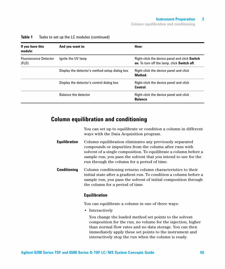
Column equilibration and conditioning
You can set up to equilibrate or condition a column in different ways with the Data Acquisition program.
Equilibration Column equilibration eliminates any previously separated compounds or impurities from the column after runs with solvent of a single composition. To equilibrate a column before a sample run, you pass the solvent that you intend to use for the run through the column for a period of time.
Conditioning Column conditioning returns column characteristics to their initial state after a gradient run. To condition a column before a sample run, you pass the solvent of initial composition through the column for a period of time.
Equilibration
You can equilibrate a column in one of three ways:
• Interactively
You change the loaded method set points to the solvent composition for the run, no volume for the injection, higher than normal flow rates and no data storage. You can then immediately apply these set points to the instrument and interactively stop the run when the column is ready.
Fluorescence Detector
(FLD)
Ignite the UV lamp Right-click the device panel and click Switch
on. To turn off the lamp, click Switch off.
Display the detector’s method setup dialog box Right-click the device panel and click
Method.
Display the detector’s control dialog box Right-click the device panel and click
Control.
Balance the detector Right-click the device panel and click
Balance.
Table 1 Tasks to set up the LC modules (continued)
If you have this
module:
And you want to: How:
Agilent 6200 Series TOF and 6500 Series Q-TOF LC/MS System Concepts Guide 55
2 Instrument Preparation
Column equilibration and conditioning
• With a method in an interactive run
You can save the method with the set points mentioned in the above paragraph, and then do a run. The run uses the method stop time. You can also use a post run time within a sample method to equilibrate the column.
For more information on worklists,
see Chapter 4, “Data Acquisition”.
• With a parameter in a worklist
You can set up a blank run in a worklist to use as your equilibration run. Or you can set up an equilibration time for any sample run, where the system waits the specified time before injecting the sample. For both cases, the data is stored.
Conditioning
You can condition a column in one of three ways:
• With one of the first two procedures described in the Equilibration paragraphs.
You enter pump conditions to bring the column to its initial condition. You can also condition the column by setting a post-run time in the method.
• With a script in a worklist
The LC conditioning script, SCP_LCCondition, is part of the Data Acquisition software. When you enter the script into the worklist, you specify the method that you will use for the run. If a TOF or Q-TOF is connected to the LC, you can also enter a parameter that diverts the LC eluent to waste. With this script, there is no injection and no data storage.
56 Agilent 6200 Series TOF and 6500 Series Q-TOF LC/MS System Concepts Guide
Instrument Preparation 2
TOF and Q-TOF preparation – calibration and tuning
TOF and Q-TOF preparation – calibration and tuning
See the Installation Guide for
instructions on how to install and
start the TOF or Q-TOF and perform
an initial tune.
After you start the instrument, you calibrate and tune the TOF and Q-TOF. This section presents the background information to help you understand calibration and tuning as they are implemented in the Agilent TOF and Q-TOF LC/MS system.
To learn how to tune and calibrate
the TOF or Q-TOF, see the Quick
Start Guide and online Help.
The following distinctions show how tuning, optimization and calibration are related in the Agilent MassHunter Workstation Software.
Tuning Tuning is the process of adjusting both the quadrupole (for the Q-TOF) and TOF parameters to achieve the following goals:
• Maximize signal intensity and maintain acceptable resolution, or
• Maximize resolution and maintain acceptable signal intensity
See “Tuning choices” on page 60
to learn more about Agilent tuning
tools.
The Agilent MassHunter Workstation software and its documentation and online Help use the words “tuning” and “optimization” interchangeably.
Agilent auto tunes for the Q-TOF include Quick Tune, Initial Tune, Mass Calibration / Check, Standard Tune, Transmission Tune, FPS System Tune, System Tune, and Set Detector Gain. Some of these tunes only work for tuning the TOF part of the instrument. Some of these auto tunes are only available on some instruments. All of the TOF auto tune tools perform both automatic calibration and tuning.
Agilent auto tune for a TOF mass spectrometer includes Initial Tune, Mass Calibration / Check, Quick Tune, Standard Tune, and Set Detector Gain.
Calibration Calibration is the process of assigning accurate masses based on the known masses of standard compounds, introduced either prior to or while running the sample.
Customizing The user interface in the Tune & Calibration tab changes based on many options:
Agilent 6200 Series TOF and 6500 Series Q-TOF LC/MS System Concepts Guide 57
2 Instrument Preparation
TOF mass calibration
• Type of mass spectrometer - Some options are only available if you have a specific instrument. For example, the SWARM tunes (Transmission Tune and System Tune) are only available for the 6530, 6545, 6545XT, and 6550 Q-TOF and 6560 IM-QTOF mass spectrometers.
• Instrument State tab - The options changed based on the parameters in the Instrument State tab. For example, the small mass auto tune options are only available if you select Low (1700 m/z) for the Mass Range and SWARM for Tuning. Also, the FPS Tune is only available if you select Enabled in the Fast Polarity Switching list.
• Preferences tab - Some tabs are only visible if you mark the appropriate option in this tab.
TOF mass calibration
Any time that you want to ensure mass accuracy of the instrument, you do a calibration. You do mass calibrations by passing a calibrant with known masses from the calibrant bottle through the mass spectrometer. You can do an automatic mass calibration, or you can do a manual mass calibration.
Automatic Mass Calibration
Before you calibrate the instrument, you have to set the instrument state to the proper instrument mode, mass range and fast polarity switching mode. You set these values on the Instrument State tab.
When you change the mass range or enable/disable fast polarity switching on the Instrument State tab, the pulser frequency is changed which results in the DEI pulser warming up or cooling down. If the calibration is performed too soon, the DEI may still be heating up or cooling down which can result in drift. See the online Help for more information on the Instrument State tab.
Automatic calibrations take place when you click Mass Calibration / Check, Quick Tune, Standard Tune,
58 Agilent 6200 Series TOF and 6500 Series Q-TOF LC/MS System Concepts Guide
Instrument Preparation 2
TOF mass calibration
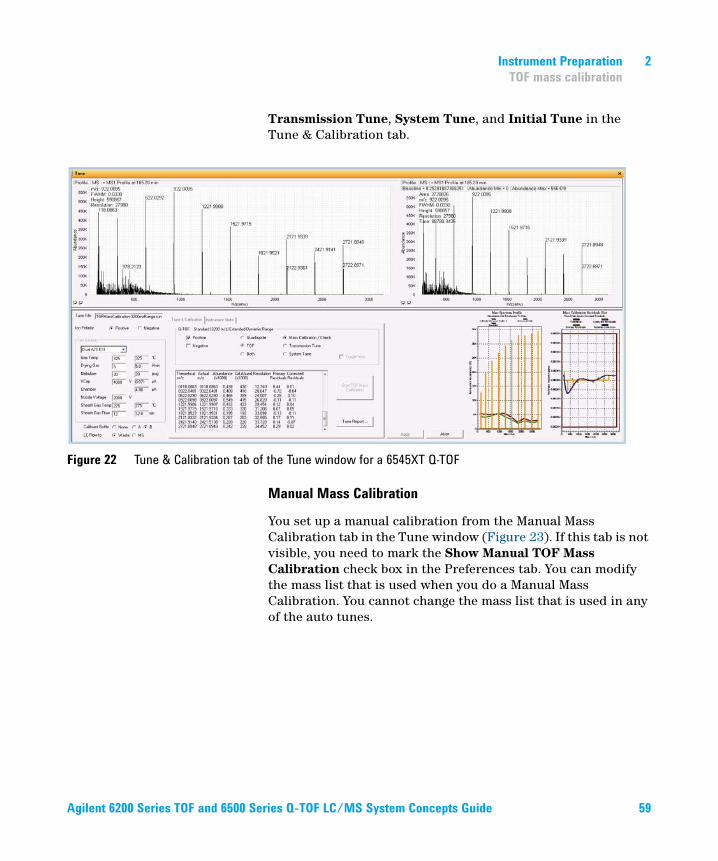
Transmission Tune, System Tune, and Initial Tune in the Tune & Calibration tab.
Figure 22 Tune & Calibration tab of the Tune window for a 6545XT Q-TOF
Manual Mass Calibration
You set up a manual calibration from the Manual Mass Calibration tab in the Tune window (Figure 23). If this tab is not visible, you need to mark the Show Manual TOF Mass Calibration check box in the Preferences tab. You can modify the mass list that is used when you do a Manual Mass Calibration. You cannot change the mass list that is used in any of the auto tunes.
Agilent 6200 Series TOF and 6500 Series Q-TOF LC/MS System Concepts Guide 59
2 Instrument Preparation
Tuning choices
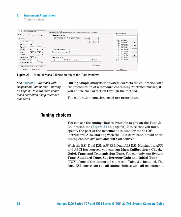
Figure 23 Manual Mass Calibration tab of the Tune window
See Chapter 3, “Methods with
Acquisition Parameters,” starting
on page 83, to learn more about
mass correction using reference
standards.
During sample analysis the system corrects the calibration with the introduction of a standard containing reference masses, if you enable the correction through the method.
The calibration equations used are proprietary.
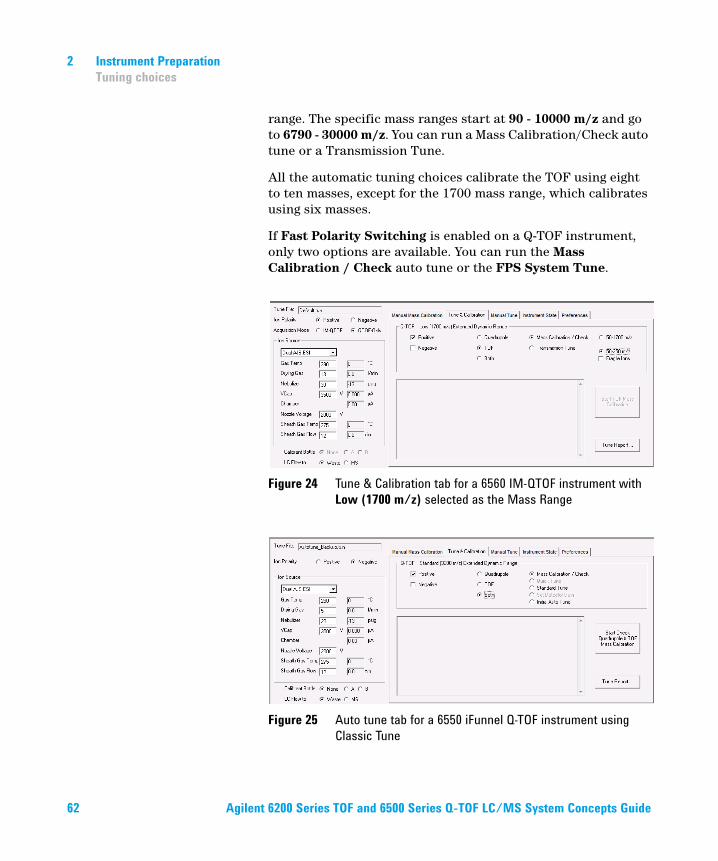
Tuning choices
You can see the tuning choices available to you on the Tune & Calibration tab (Figure 24 on page 62). Notice that you must specify the part of the instrument to tune for the Q-TOF instrument. Also, starting with the B.02.01 release, not all of the tuning choices are available with all sources.
With the ESI, Dual ESI, AJS ESI, Dual AJS ESI, Multimode, APPI and APCI ion sources, you can run Mass Calibration / Check, Quick Tune, and Transmission Tune. You can only run System Tune, Standard Tune, Set Detector Gain and Initial Tune (TOF) if one of the supported sources in Table 2 is installed. The Dual ESI source can run all tuning choices with all instruments.
60 Agilent 6200 Series TOF and 6500 Series Q-TOF LC/MS System Concepts Guide
Instrument Preparation 2
Tuning choices
Also, the Instrument Mode affects which autotunes are available to use. If the Instrument Mode is Extended Dynamic Range (2 GHz) mode, then you can perform any of the autotunes. If the Instrument Mode is not Extended Dynamic Range mode, then you cannot perform the Initial Tune. You set the Instrument Mode on the Instrument State tab.
The Mass Range also affects which tunes are supported. You can run all tunes if the Mass Range is Standard (3200 m/z). If the Mass Range is Low (1700 m/z), you cannot run an Initial Tune or a Set Detector Gain.
For the 6530, 6545, 6545XT, 6550, and 6560 LC/MS instruments, if you select Low (1700 m/z) for the Mass Range, then you have multiple options to tune for this Mass Range, plus an option to tune for Fragile Ions for the low Mass Range, if you select either 50-750 m/z (6545 and 6545XT only) or 50-250 m/z.
For all other instruments, for small molecule application, do an additional Quad Tune in the 1700 m/z range to increase performance for molecules < 300 m/z.
For the 6545XT, if you select High (10K - 30K m/z) for the Mass Range, then you use the slider to select the specific high mass
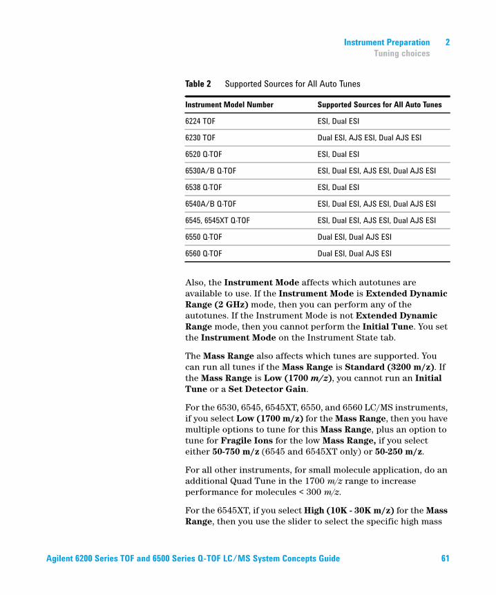
Table 2 Supported Sources for All Auto Tunes
Instrument Model Number Supported Sources for All Auto Tunes
6224 TOF ESI, Dual ESI
6230 TOF Dual ESI, AJS ESI, Dual AJS ESI
6520 Q-TOF ESI, Dual ESI
6530A/B Q-TOF ESI, Dual ESI, AJS ESI, Dual AJS ESI
6538 Q-TOF ESI, Dual ESI
6540A/B Q-TOF ESI, Dual ESI, AJS ESI, Dual AJS ESI
6545, 6545XT Q-TOF ESI, Dual ESI, AJS ESI, Dual AJS ESI
6550 Q-TOF Dual ESI, Dual AJS ESI
6560 Q-TOF Dual ESI, Dual AJS ESI
Agilent 6200 Series TOF and 6500 Series Q-TOF LC/MS System Concepts Guide 61
2 Instrument Preparation
Tuning choices
range. The specific mass ranges start at 90 - 10000 m/z and go to 6790 - 30000 m/z. You can run a Mass Calibration/Check auto tune or a Transmission Tune.
All the automatic tuning choices calibrate the TOF using eight to ten masses, except for the 1700 mass range, which calibrates using six masses.
If Fast Polarity Switching is enabled on a Q-TOF instrument, only two options are available. You can run the Mass Calibration / Check auto tune or the FPS System Tune.
Figure 24 Tune & Calibration tab for a 6560 IM-QTOF instrument with
Low (1700 m/z) selected as the Mass Range
Figure 25 Auto tune tab for a 6550 iFunnel Q-TOF instrument using
Classic Tune
62 Agilent 6200 Series TOF and 6500 Series Q-TOF LC/MS System Concepts Guide
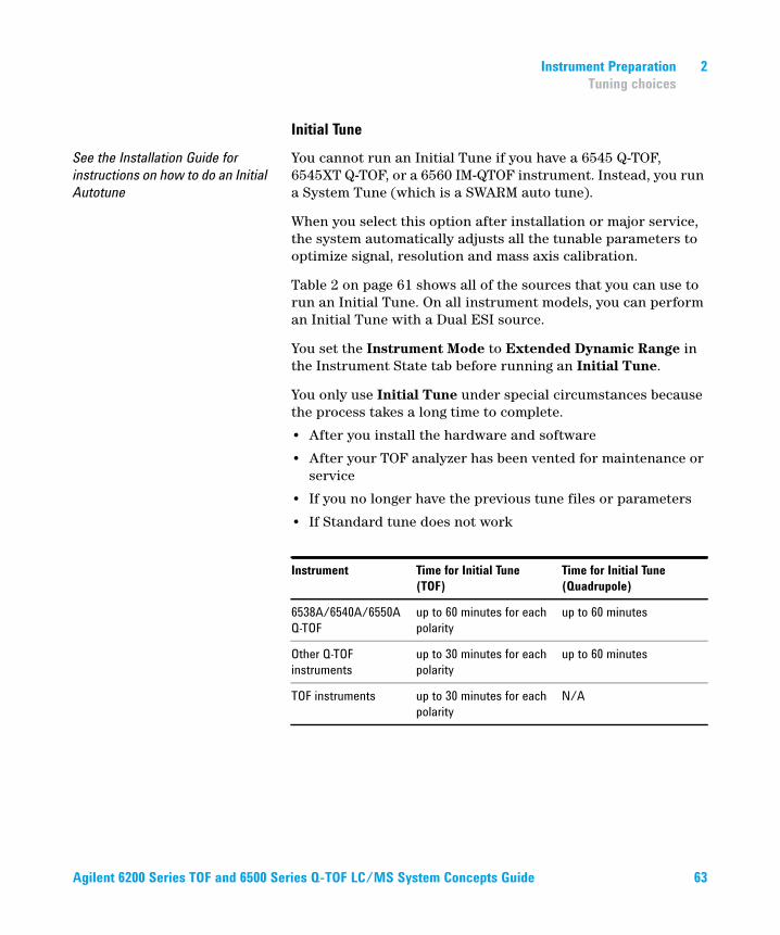
Instrument Preparation 2
Tuning choices
Initial Tune
See the Installation Guide for
instructions on how to do an Initial
Autotune
You cannot run an Initial Tune if you have a 6545 Q-TOF, 6545XT Q-TOF, or a 6560 IM-QTOF instrument. Instead, you run a System Tune (which is a SWARM auto tune).
When you select this option after installation or major service, the system automatically adjusts all the tunable parameters to optimize signal, resolution and mass axis calibration.
Table 2 on page 61 shows all of the sources that you can use to run an Initial Tune. On all instrument models, you can perform an Initial Tune with a Dual ESI source.
You set the Instrument Mode to Extended Dynamic Range in the Instrument State tab before running an Initial Tune.
You only use Initial Tune under special circumstances because the process takes a long time to complete.
• After you install the hardware and software
• After your TOF analyzer has been vented for maintenance or service
• If you no longer have the previous tune files or parameters
• If Standard tune does not work
Instrument Time for Initial Tune
(TOF)
Time for Initial Tune
(Quadrupole)
6538A/6540A/6550A
Q-TOF
up to 60 minutes for each
polarity
up to 60 minutes
Other Q-TOF
instruments
up to 30 minutes for each
polarity
up to 60 minutes
TOF instruments up to 30 minutes for each
polarity
N/A
Agilent 6200 Series TOF and 6500 Series Q-TOF LC/MS System Concepts Guide 63
2 Instrument Preparation
Tuning choices
During the Initial Tune process for the TOF, the system goes through the following steps without your intervention.
a Resets any current tune parameters to original defaults
b Performs a coarse TOF mass axis calibration
c Adjusts all the tunable parameters automatically
d Performs a final TOF mass axis calibration
e Prints a tune report at the end of the auto tune process
Collision Cell
gas pressure
For Q-TOF instruments except for the 6545, 6545XT, and 6560, after running an Initial Tune (TOF), you need to adjust the Collision Cell Gas pressure. You can find this procedure in the installation manual. For the 6545, 6545XT, and the 6560 with Positive polarity, the Collision Cell gas pressure is adjusted automatically after a Quad or Q-TOF system tune.
During the Initial Tune process for the quadrupole, the system goes through steps a, c, d and e.
Mass Calibration / Check
You can perform a Mass Calibration / Check with any instrument mode selected and with any of the following sources installed:
• ESI
• AJS ESI (Agilent Jet Stream ESI)
• Dual ESI
• Dual AJS ESI (Dual Agilent Jet Stream ESI)
• MMI
• APPI
• APCI
Agilent designed the instrument so that it does not need frequent autotunes. Periodically, you may want to perform Mass Calibration / Check on both the TOF and the Quadrupole to ensure that the parameters are still optimized. You do not need to perform a Calibration / Check on the Quadrupole as often as a Calibration / Check on the TOF.
64 Agilent 6200 Series TOF and 6500 Series Q-TOF LC/MS System Concepts Guide
Instrument Preparation 2
Tuning choices
Standard Tune
You cannot run a Standard Tune if you have a 6545 Q-TOF, a 6545XT Q-TOF, or a 6560 IM-QTOF instrument. Instead, you run a System Tune or a Transmission Tune.
These tools perform many of the same optimization operations as the Initial Tune tools but use the current settings as starting values and do a limited set of ion optic ramps.
Table 2 on page 61 shows all of the sources that you can use to run a Standard Tune. On all instrument models, you can perform a Standard Tune with a Dual ESI source.
The Standard Tune for the Quadrupole and for the TOF part of the instrument do subsets of the Initial Tune actions, and they use the current tune parameters as starting points rather than using the factory defaults.
Standard Tune on the TOF takes about 10 to 15 minutes, and Standard Tune on the Quadrupole takes about 10 to 15 minutes to complete.
Quick Tune (TOF)
You cannot run a Quick Tune if you have a 6545 Q-TOF, a 6545XT Q-TOF, or a 6560 IM-QTOF instrument.
Quick Tune on the TOF part of the instrument automatically adjusts the most commonly required subset of tunable parameters.
You can perform a Quick Tune with any instrument mode selected and with any of the following sources installed:
• ESI
• AJS ESI (Agilent Jet Stream ESI)
• Dual ESI
• Dual AJS ESI (Dual Agilent Jet Stream ESI)
• MMI
• APPI
• APCI
Agilent 6200 Series TOF and 6500 Series Q-TOF LC/MS System Concepts Guide 65
2 Instrument Preparation
Tuning choices
Quick Tune takes 3 to 5 minutes because the software is optimizing only the most significant parameters followed by a calibration. You cannot select this option if you have selected either Quadrupole or Both as the part of the instrument to tune.
During Quick Tune the system goes through the following steps:
a Automatically opens the calibrant valve
b Adjusts the vertical Q (Vert Q) and bottom slit parameters in the Beam Shaping Optics (optimizes transmission)
c Adjusts the middle mirror of the compound TOF ion mirror (optimizes resolution)
d Does a mass axis calibration after the final adjustment
e Prints a tune report
Set Detector Gain
You can run a Set Detector Gain on all instruments.
Set Detector Gain adjusts the PMT voltage to obtain consistent gain (amplification) of the ion current into electrical current. In the Extended Dynamic Range (2 GHz) mode, it also adjusts the preamp offset values and the time delay between gain channels. This tool is a subset of Initial Tune. You can only select this option if you click TOF as the part of the instrument to tune.
Table 2 on page 61 shows all of the sources that you can use to run a Set Detector Gain. On all instrument models, you can perform a Set Detector Gain with a Dual ESI source.
You set the Instrument Mode to Extended Dynamic Range (2 GHz) in the Instrument State tab before running the Set Detector Gain algorithm.
66 Agilent 6200 Series TOF and 6500 Series Q-TOF LC/MS System Concepts Guide
Instrument Preparation 2
Tuning choices
SWARM Tune - System Tune or Transmission Tune
The 6545 Q-TOF, the 6545XT Q-TOF, and the 6560 IM-QTOF mass spectrometers use a different tune algorithm. The 6530 Q-TOF and the 6550 Q-TOF can use either the Classic auto tune or the SWARM tune. The new auto tune uses both Particle Swarm Optimization (PSO) and a simplex algorithm within the physical constraints of the mass spectrometer.
• For a well-known parameter, the auto tune uses the simplex algorithm to maximize speed.
• For unknown behavior, PSO is used.
• PSO and simplex are interchanged between coarse and fine adjustment.
• All the parameters are bound within the knowledge of ion physics, to limit the search space.
• The theory of mass spectrometry is built into the algorithm so that no ion storage or ion blocking occurs during optimization.
During TOF resolution tuning, a certain abundance amount is sacrificed to reach the target resolution. For the parameters where resolution and sensitivity go together, the decision is easy to make. For parameters where resolution and sensitivity are inversely proportional, a compromise is needed. The general rule is that for a one percent increase in resolution you sacrifice four percent in sensitivity.
For example, if resolution goes from 27000 to 30000 (10% increase), the algorithm will sacrifice the intensity up to 31%
• Setting 1: gives 27000 Resolution and 1.00 M Peak Height
• Setting 2: gives 30000 Resolution and 0.70 M Peak Height
• Setting 3: gives 30000 Resolution and 0.68 M Peak Height
Between setting 1 and setting 2, the algorithm picks setting 2.
Between setting 1 and setting 3, the algorithm picks setting 1.
If you select Low (1700 m/z) for the Mass Range, then you have additional low mass tune options. You can select a smaller range to use when tuning. If you select either 50-750 m/z (only
Agilent 6200 Series TOF and 6500 Series Q-TOF LC/MS System Concepts Guide 67
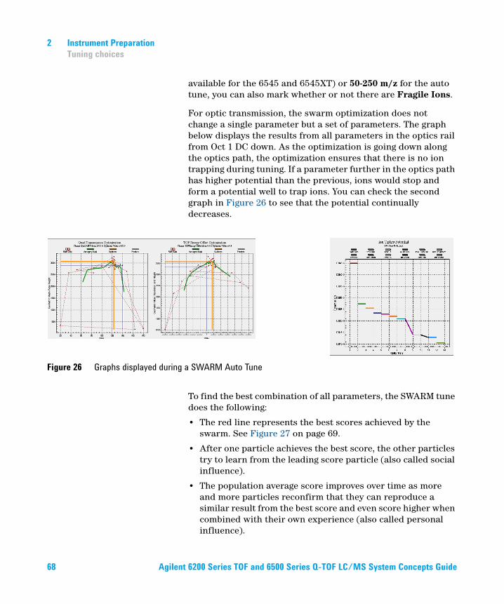
2 Instrument Preparation
Tuning choices
available for the 6545 and 6545XT) or 50-250 m/z for the auto tune, you can also mark whether or not there are Fragile Ions.
For optic transmission, the swarm optimization does not change a single parameter but a set of parameters. The graph below displays the results from all parameters in the optics rail from Oct 1 DC down. As the optimization is going down along the optics path, the optimization ensures that there is no ion trapping during tuning. If a parameter further in the optics path has higher potential than the previous, ions would stop and form a potential well to trap ions. You can check the second graph in Figure 26 to see that the potential continually decreases.
To find the best combination of all parameters, the SWARM tune does the following:
• The red line represents the best scores achieved by the swarm. See Figure 27 on page 69.
• After one particle achieves the best score, the other particles try to learn from the leading score particle (also called social influence).
• The population average score improves over time as more and more particles reconfirm that they can reproduce a similar result from the best score and even score higher when combined with their own experience (also called personal influence).
Figure 26 Graphs displayed during a SWARM Auto Tune
68 Agilent 6200 Series TOF and 6500 Series Q-TOF LC/MS System Concepts Guide
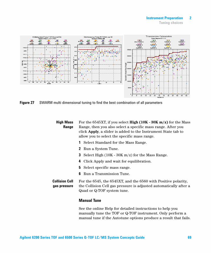
Instrument Preparation 2
Tuning choices
High Mass
Range
For the 6545XT, if you select High (10K - 30K m/z) for the Mass Range, then you also select a specific mass range. After you click Apply, a slider is added to the Instrument State tab to allow you to select the specific mass range.
1 Select Standard for the Mass Range.
2 Run a System Tune.
3 Select High (10K - 30K m/z) for the Mass Range.
4 Click Apply and wait for equilibration.
5 Select specific mass range.
6 Run a Transmission Tune.
Collision Cell
gas pressure
For the 6545, the 6545XT, and the 6560 with Positive polarity, the Collision Cell gas pressure is adjusted automatically after a Quad or Q-TOF system tune.
Manual Tune
See the online Help for detailed instructions to help you manually tune the TOF or Q-TOF instrument. Only perform a manual tune if the Autotune options produce a result that fails.
Figure 27 SWARM multi dimensional tuning to find the best combination of all parameters
Agilent 6200 Series TOF and 6500 Series Q-TOF LC/MS System Concepts Guide 69
2 Instrument Preparation
Tuning choices
Order of using Autotune choices
for Classic
Autotune
Use the tuning options in the following order:
1 Mass Calibration / Check tune for the TOF
If necessary, continue.
2 Quick Tune for the TOF (does not exist for the quadrupole)
If necessary, continue.
3 Standard Tune for the TOF and Quadrupole - You must select Standard (3200 m/z) for the Mass Range and High Resolution for the Slicer Mode.
If necessary, continue.
4 Initial Tune for the TOF and Quadrupole
If an Initial Tune cannot complete, contact Agilent Support.
for SWARM
Auto Tune
(6530 Q-TOF,
6545 Q-TOF,
6545XT Q-TOF,
or 6560
IM-QTOF)
Use the tuning options in the following order:
1 Mass Calibration / Check tune for the Q-TOF
If necessary, continue.
2 Transmission Tune (if you selected Low (1700 m/z) for the Mass Range). You can try successively higher mass ranges.
If necessary, continue.
3 System Tune - You must select Standard (3200 m/z) for the Mass Range and High Resolution for the Slicer Mode.
If the System Tune cannot complete, contact Agilent Support.
70 Agilent 6200 Series TOF and 6500 Series Q-TOF LC/MS System Concepts Guide

Instrument Preparation 2
Tune reports
Tune reports
At the end of every Check Tune, Quick Tune, Standard Tune, Initial Tune, Transmission Tune, or System Tune, the system generates a printable Tune report. The TOF and Quad tune reports let you know if optimization limits are met. For a TOF tune, the report also lets you know if the mass calibration is satisfactory or not. To print previous tune reports, you click the Tune Report button in the Tune & Calibration tab.
Agilent 6200 Series TOF and 6500 Series Q-TOF LC/MS System Concepts Guide 71
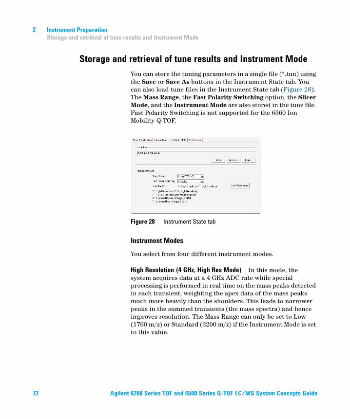
2 Instrument Preparation
Storage and retrieval of tune results and Instrument Mode
Storage and retrieval of tune results and Instrument Mode
You can store the tuning parameters in a single file (*.tun) using the Save or Save As buttons in the Instrument State tab. You can also load tune files in the Instrument State tab (Figure 28). The Mass Range, the Fast Polarity Switching option, the Slicer Mode, and the Instrument Mode are also stored in the tune file. Fast Polarity Switching is not supported for the 6560 Ion Mobility Q-TOF.
Instrument Modes
You select from four different instrument modes.
High Resolution (4 GHz, High Res Mode) In this mode, the system acquires data at a 4 GHz ADC rate while special processing is performed in real time on the mass peaks detected in each transient, weighting the apex data of the mass peaks much more heavily than the shoulders. This leads to narrower peaks in the summed transients (the mass spectra) and hence improves resolution. The Mass Range can only be set to Low (1700 m/z) or Standard (3200 m/z) if the Instrument Mode is set to this value.
Figure 28 Instrument State tab
72 Agilent 6200 Series TOF and 6500 Series Q-TOF LC/MS System Concepts Guide
Instrument Preparation 2
Storage and retrieval of tune results and Instrument Mode
4 GHz (High Resolution Mode disabled) In this mode, no processing is used at the transient level; however, the system acquires data at a 4 GHz ADC rate. The Mass Range can only be set to Low (1700 m/z) or Standard (3200 m/z) if the Instrument Mode is set to this value.
Extended Dynamic Range (2 GHz) In this mode, the system acquires data at a 4 GHz ADC rate in dual channel mode. One channel is recorded at a high detector gain while the other channel operates at a low detector gain. The firmware stitches the two channels together to produce a scan with a sampling rate of 2 GHz, which results in a greatly increased dynamic range. The Mass Range can only be set to Low (1700 m/z) or Standard (3200 m/z) if the Instrument Mode is set to this value.
Extended Mass Range (2 GHz) In this mode, the system acquires data at a 2 GHz ADC rate. The Mass Range can be set to Low (1700 m/z), Standard (3200 m/z), or High (10,000). This is the only mode that you can use with the highest mass range.
Agilent 6200 Series TOF and 6500 Series Q-TOF LC/MS System Concepts Guide 73
2 Instrument Preparation
Tune Set Point Modifications for Medium and Large Proteins
Tune Set Point Modifications for Medium and Large Proteins
If you have a 6545XT, you run the large molecule SWARM tune in extended mass range to tune for medium and large proteins; this tune performs all necessary steps.
If you are using SWARM auto tune with 6530, 6545, 6545XT, 6550, or 6560 Q-TOF, these steps are done automatically during the auto tune.
If you have a 6520 or 6530 Q-TOF and are using Classic tune, then for medium and large proteins, the charge envelope may extend beyond 3200 m/z. Agilent recommends that you acquire your intact protein data in the Extended Mass Range (2 GHz) mode on the 6200 Series TOF and 6520/6530 Q-TOF as this allows the extended mass range needed for larger proteins. If you are acquiring a protein and the charge states are “cut-off” in one of the other modes, you can switch to this mode with the extended mass range.
If you are acquiring medium and large protein data, Agilent also recommends that the Quad AMU be raised to 300 amu instead of using the value established by the Auto Tune algorithm. This action provides the Quad with enough power to transmit the high mass ions through the quad. Failure to increase the Quad AMU will result in a mass spectrum where the charge envelope appears to be “cutoff” for the higher charge state ion clusters.
To adjust the Quad AMU, do the following steps:
1 Switch to the Tune Context.
2 Click the Manual Tune tab.
3 Click the Quad Tab.
4 For the Quad AMU, type 300 for the new value.
5 Save the tune value to save the new Quad AMU value. Then exit the Tune Context.
74 Agilent 6200 Series TOF and 6500 Series Q-TOF LC/MS System Concepts Guide
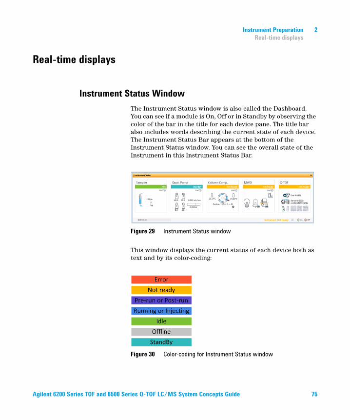
Instrument Preparation 2
Real-time displays
Real-time displays
Instrument Status Window
The Instrument Status window is also called the Dashboard. You can see if a module is On, Off or in Standby by observing the color of the bar in the title for each device pane. The title bar also includes words describing the current state of each device. The Instrument Status Bar appears at the bottom of the Instrument Status window. You can see the overall state of the Instrument in this Instrument Status Bar.
This window displays the current status of each device both as text and by its color-coding:
Figure 29 Instrument Status window
Figure 30 Color-coding for Instrument Status window
Agilent 6200 Series TOF and 6500 Series Q-TOF LC/MS System Concepts Guide 75
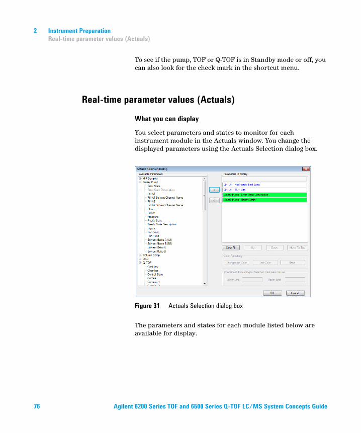
2 Instrument Preparation
Real-time parameter values (Actuals)
To see if the pump, TOF or Q-TOF is in Standby mode or off, you can also look for the check mark in the shortcut menu.
Real-time parameter values (Actuals)
What you can display
You select parameters and states to monitor for each instrument module in the Actuals window. You change the displayed parameters using the Actuals Selection dialog box.
The parameters and states for each module listed below are available for display.
Figure 31 Actuals Selection dialog box
76 Agilent 6200 Series TOF and 6500 Series Q-TOF LC/MS System Concepts Guide
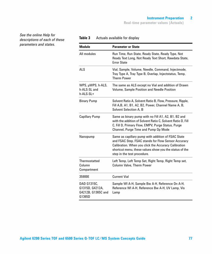
Instrument Preparation 2
Real-time parameter values (Actuals)
See the online Help for
descriptions of each of these
parameters and states.
Table 3 Actuals available for display
Module Parameter or State
All modules Run Time, Run State, Ready State, Ready Type, Not
Ready Text Long, Not Ready Text Short, Rawdata State,
Error State
ALS Vial, Sample, Volume, Needle, Command, Injectmode,
Tray Type A, Tray Type B, Overlap, Injectstatus, Temp,
Therm Power
WPS, µWPS, h-ALS,
h-ALS-SL and
h-ALS-SL+
The same as ALS except no Vial and addition of Drawn
Volume, Sample Position and Needle Position
Binary Pump Solvent Ratio A, Solvent Ratio B, Flow, Pressure, Ripple,
Fill A,B, A1, B1, A2, B2, Power, Channel Name A, B,
Solvent Selection A, B
Capillary Pump Same as binary pump with no Fill A1, A2, B1, B2 and
with the addition of Solvent Ratio C, Solvent Ratio D, Fill
C, Fill D, Primary Flow, EMPV, Purge Status, Purge
Channel, Purge Time and Pump Op Mode
Nanopump Same as capillary pump with addition of FSAC State
and FSAC Step. FSAC stands for Flow Sensor Accuracy
Calibration. When you click the Accuracy Calibration
shortcut menu, these values show you the status of the
step in the test procedure.
Thermostatted
Column
Compartment
Left Temp, Left Temp Set, Right Temp, Right Temp set,
Column Valve, Therm Power
35900E Current Vial
DAD G1315C,
G1315D, G4212A,
G4212B, G1365C and
G1365D
Sample Wl A-H, Sample Bw A-H, Reference On A-H,
Reference Wl A-H, Reference Bw A-H, UV Lamp, Vis
Lamp
Agilent 6200 Series TOF and 6500 Series Q-TOF LC/MS System Concepts Guide 77
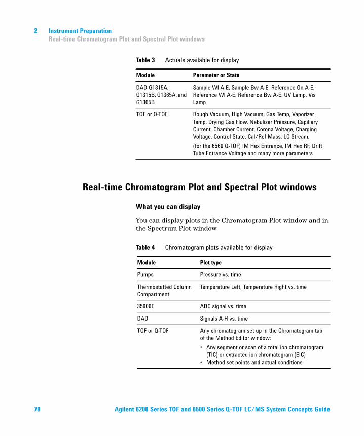
2 Instrument Preparation
Real-time Chromatogram Plot and Spectral Plot windows
Real-time Chromatogram Plot and Spectral Plot windows
What you can display
You can display plots in the Chromatogram Plot window and in the Spectrum Plot window.
DAD G1315A,
G1315B, G1365A, and
G1365B
Sample Wl A-E, Sample Bw A-E, Reference On A-E,
Reference Wl A-E, Reference Bw A-E, UV Lamp, Vis
Lamp
TOF or Q-TOF Rough Vacuum, High Vacuum, Gas Temp, Vaporizer
Temp, Drying Gas Flow, Nebulizer Pressure, Capillary
Current, Chamber Current, Corona Voltage, Charging
Voltage, Control State, Cal/Ref Mass, LC Stream,
(for the 6560 Q-TOF) IM Hex Entrance, IM Hex RF, Drift
Tube Entrance Voltage and many more parameters
Table 3 Actuals available for display
Module Parameter or State
Table 4 Chromatogram plots available for display
Module Plot type
Pumps Pressure vs. time
Thermostatted Column
Compartment
Temperature Left, Temperature Right vs. time
35900E ADC signal vs. time
DAD Signals A-H vs. time
TOF or Q-TOF Any chromatogram set up in the Chromatogram tab
of the Method Editor window:
• Any segment or scan of a total ion chromatogram
(TIC) or extracted ion chromatogram (EIC)
• Method set points and actual conditions
78 Agilent 6200 Series TOF and 6500 Series Q-TOF LC/MS System Concepts Guide
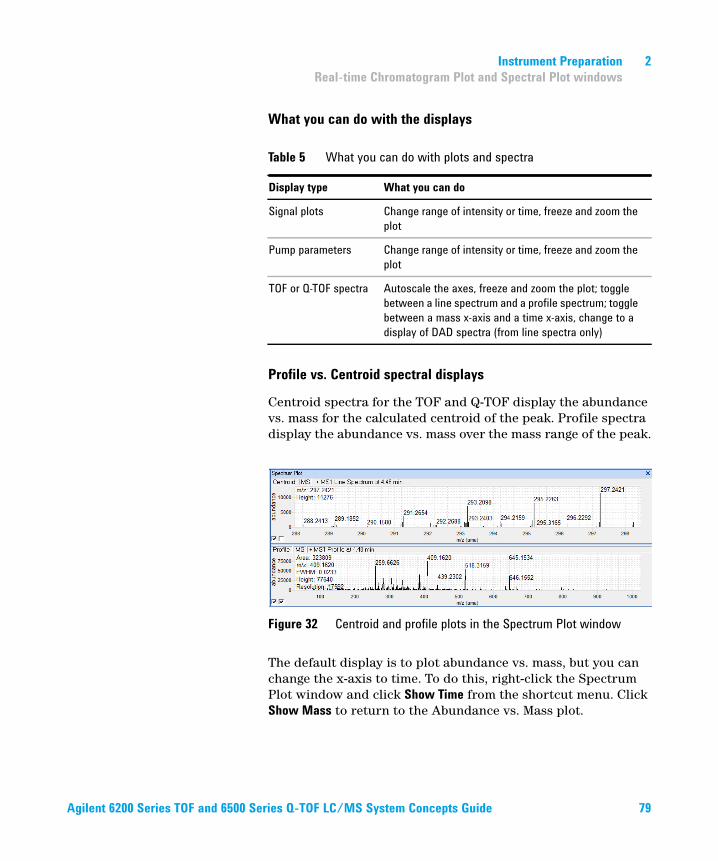
Instrument Preparation 2
Real-time Chromatogram Plot and Spectral Plot windows
What you can do with the displays
Profile vs. Centroid spectral displays
Centroid spectra for the TOF and Q-TOF display the abundance vs. mass for the calculated centroid of the peak. Profile spectra display the abundance vs. mass over the mass range of the peak.
The default display is to plot abundance vs. mass, but you can change the x-axis to time. To do this, right-click the Spectrum Plot window and click Show Time from the shortcut menu. Click Show Mass to return to the Abundance vs. Mass plot.
Table 5 What you can do with plots and spectra
Display type What you can do
Signal plots Change range of intensity or time, freeze and zoom the
plot
Pump parameters Change range of intensity or time, freeze and zoom the
plot
TOF or Q-TOF spectra Autoscale the axes, freeze and zoom the plot; toggle
between a line spectrum and a profile spectrum; toggle
between a mass x-axis and a time x-axis, change to a
display of DAD spectra (from line spectra only)
Figure 32 Centroid and profile plots in the Spectrum Plot window
Agilent 6200 Series TOF and 6500 Series Q-TOF LC/MS System Concepts Guide 79
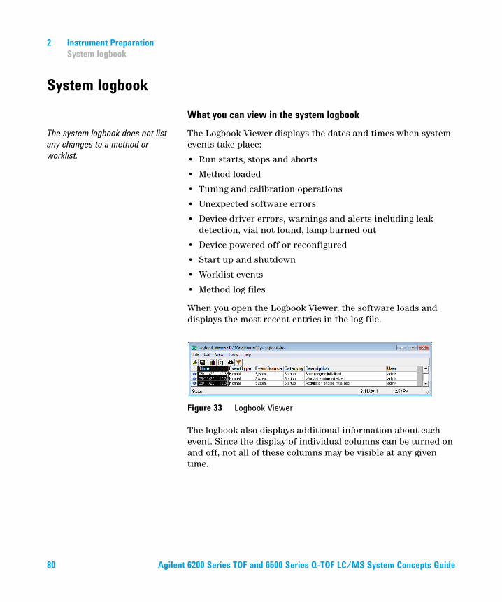
2 Instrument Preparation
System logbook
System logbook
What you can view in the system logbook
The system logbook does not list
any changes to a method or
worklist.
The Logbook Viewer displays the dates and times when system events take place:
• Run starts, stops and aborts
• Method loaded
• Tuning and calibration operations
• Unexpected software errors
• Device driver errors, warnings and alerts including leak detection, vial not found, lamp burned out
• Device powered off or reconfigured
• Start up and shutdown
• Worklist events
• Method log files
When you open the Logbook Viewer, the software loads and displays the most recent entries in the log file.
Figure 33 Logbook Viewer
The logbook also displays additional information about each event. Since the display of individual columns can be turned on and off, not all of these columns may be visible at any given time.
80 Agilent 6200 Series TOF and 6500 Series Q-TOF LC/MS System Concepts Guide
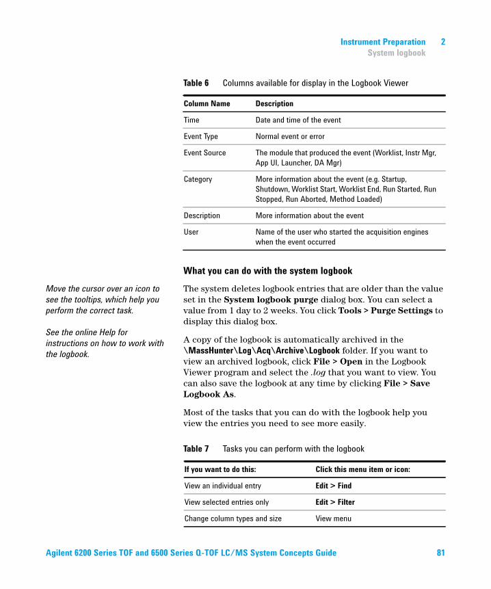
Instrument Preparation 2
System logbook
What you can do with the system logbook
Move the cursor over an icon to
see the tooltips, which help you
perform the correct task.
See the online Help for
instructions on how to work with
the logbook.
The system deletes logbook entries that are older than the value set in the System logbook purge dialog box. You can select a value from 1 day to 2 weeks. You click Tools > Purge Settings to display this dialog box.
A copy of the logbook is automatically archived in the \MassHunter\Log\Acq\Archive\Logbook folder. If you want to view an archived logbook, click File > Open in the Logbook Viewer program and select the .log that you want to view. You can also save the logbook at any time by clicking File > Save Logbook As.
Most of the tasks that you can do with the logbook help you view the entries you need to see more easily.
Table 6 Columns available for display in the Logbook Viewer
Column Name Description
Time Date and time of the event
Event Type Normal event or error
Event Source The module that produced the event (Worklist, Instr Mgr,
App UI, Launcher, DA Mgr)
Category More information about the event (e.g. Startup,
Shutdown, Worklist Start, Worklist End, Run Started, Run
Stopped, Run Aborted, Method Loaded)
Description More information about the event
User Name of the user who started the acquisition engines
when the event occurred
Table 7 Tasks you can perform with the logbook
If you want to do this: Click this menu item or icon:
View an individual entry Edit > Find
View selected entries only Edit > Filter
Change column types and size View menu
Agilent 6200 Series TOF and 6500 Series Q-TOF LC/MS System Concepts Guide 81
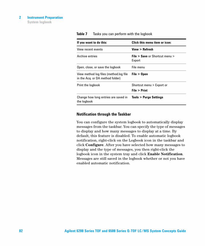
2 Instrument Preparation
System logbook
Notification through the Taskbar
You can configure the system logbook to automatically display messages from the taskbar. You can specify the type of messages to display and how many messages to display at a time. By default, this feature is disabled. To enable automatic logbook notification, right-click on the Logbook icon in the taskbar and click Configure. After you have selected how many messages to display and the type of messages, you then right-click the logbook icon in the system tray and click Enable Notification. Messages are still saved in the logbook whether or not you have enabled automatic notification.
View recent events View > Refresh
Archive entries File > Save or Shortcut menu >
Export
Open, close, or save the logbook File menu
View method log files (method.log file
in the Acq. or DA method folder)
File > Open
Print the logbook Shortcut menu > Export or
File > Print
Change how long entries are saved in
the logbook
Tools > Purge Settings
Table 7 Tasks you can perform with the logbook
If you want to do this: Click this menu item or icon:
82 Agilent 6200 Series TOF and 6500 Series Q-TOF LC/MS System Concepts Guide
Agilent 6200 Series TOF and 6500 Series Q-TOF LC/MS System
3Methods with Acquisition Parameters
Parameter entry 84
General TOF and Q-TOF parameters 87
TOF and Q-TOF acquisition parameters 91
Ion source parameters 89
Setup of TOF and Q-TOF reference mass correction (recalibration) 100
TOF and Q-TOF chromatogram setup 104
Q-TOF Advanced Parameters for Ion Mobility 105
Setting parameters to acquire a data file in All Ions MS/MS
mode 108
Setting parameters on a 6560 IM-QTOF to acquire a data file in All Ions
MS/MS mode 111
Method saving, editing and reporting 112
Saving a method with data acquisition parameters 112
Method editing 114
Method reporting 115
See the online Help for
instructions on setting up methods
and parameter descriptions.
You use this chapter to learn about the concepts that can help you set up methods containing data acquisition parameters.
83
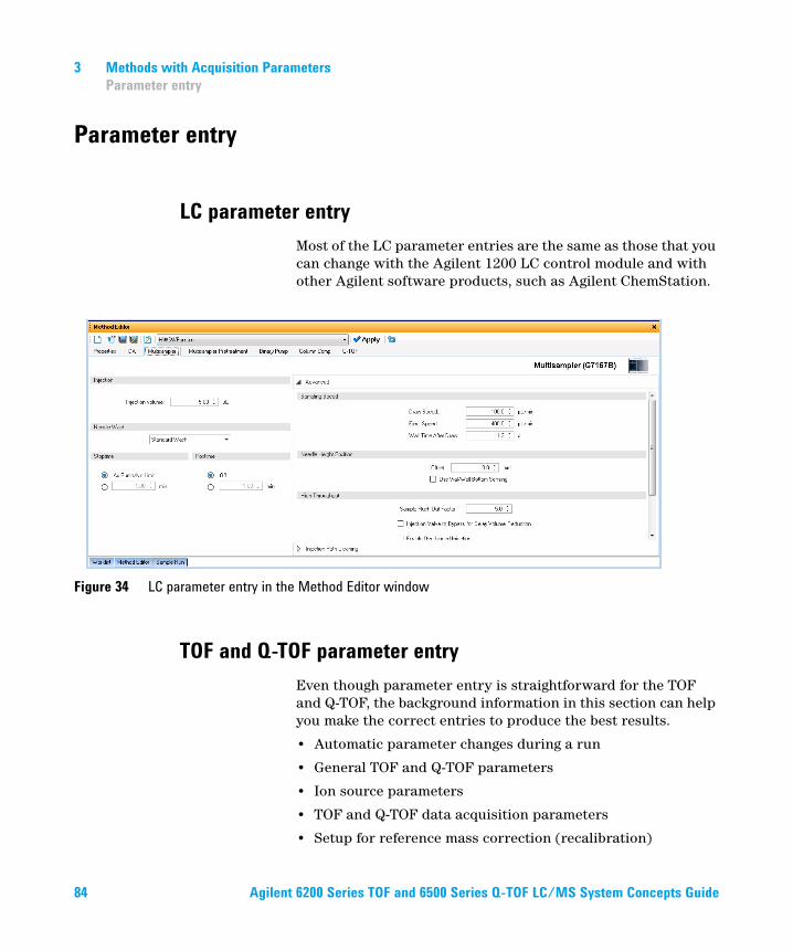
3 Methods with Acquisition Parameters
Parameter entry
Parameter entry
LC parameter entry
Most of the LC parameter entries are the same as those that you can change with the Agilent 1200 LC control module and with other Agilent software products, such as Agilent ChemStation.
TOF and Q-TOF parameter entry
Even though parameter entry is straightforward for the TOF and Q-TOF, the background information in this section can help you make the correct entries to produce the best results.
• Automatic parameter changes during a run
• General TOF and Q-TOF parameters
• Ion source parameters
• TOF and Q-TOF data acquisition parameters
• Setup for reference mass correction (recalibration)
Figure 34 LC parameter entry in the Method Editor window
84 Agilent 6200 Series TOF and 6500 Series Q-TOF LC/MS System Concepts Guide
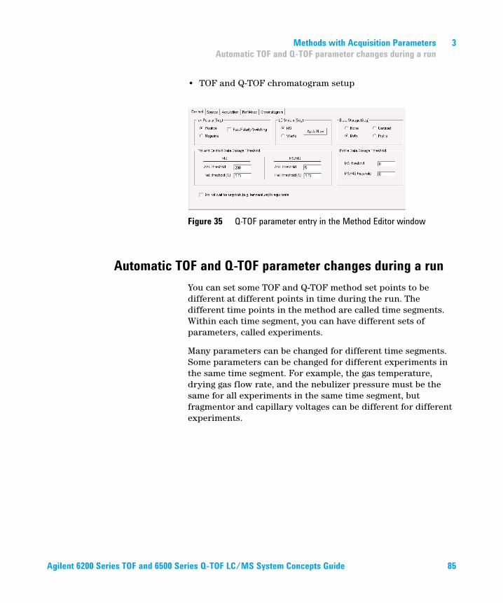
Methods with Acquisition Parameters 3
Automatic TOF and Q-TOF parameter changes during a run
• TOF and Q-TOF chromatogram setup
Automatic TOF and Q-TOF parameter changes during a run
You can set some TOF and Q-TOF method set points to be different at different points in time during the run. The different time points in the method are called time segments. Within each time segment, you can have different sets of parameters, called experiments.
Many parameters can be changed for different time segments. Some parameters can be changed for different experiments in the same time segment. For example, the gas temperature, drying gas flow rate, and the nebulizer pressure must be the same for all experiments in the same time segment, but fragmentor and capillary voltages can be different for different experiments.
Figure 35 Q-TOF parameter entry in the Method Editor window
Agilent 6200 Series TOF and 6500 Series Q-TOF LC/MS System Concepts Guide 85
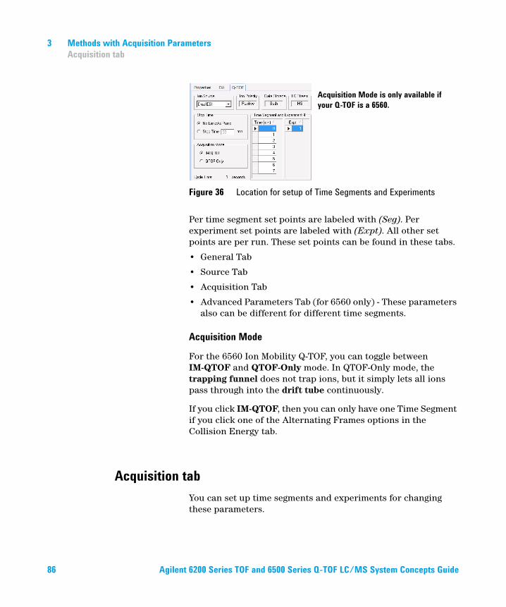
3 Methods with Acquisition Parameters
Acquisition tab
Per time segment set points are labeled with (Seg). Per experiment set points are labeled with (Expt). All other set points are per run. These set points can be found in these tabs.
• General Tab
• Source Tab
• Acquisition Tab
• Advanced Parameters Tab (for 6560 only) - These parameters also can be different for different time segments.
Acquisition Mode
For the 6560 Ion Mobility Q-TOF, you can toggle between IM-QTOF and QTOF-Only mode. In QTOF-Only mode, the trapping funnel does not trap ions, but it simply lets all ions pass through into the drift tube continuously.
If you click IM-QTOF, then you can only have one Time Segment if you click one of the Alternating Frames options in the Collision Energy tab.
Acquisition tab
You can set up time segments and experiments for changing these parameters.
Figure 36 Location for setup of Time Segments and Experiments
Acquisition Mode is only available if
your Q-TOF is a 6560.
86 Agilent 6200 Series TOF and 6500 Series Q-TOF LC/MS System Concepts Guide
Methods with Acquisition Parameters 3
General TOF and Q-TOF parameters
MS mode The MS mode spectral parameters can be set for each time segment, and the Collision Energy parameters can be set for each experiment.
• Q-TOF Spectral Parameters Tab - for each time segment
• Q-TOF Collision Energy Tab - for each experiment
Auto MS/MS mode (Q-TOF only) The parameters on the following tabs can be set for each time segment.
• Q-TOF Spectral Parameters Tab
• Q-TOF Collision Energy Tab
• Q-TOF Precursor Selection I Tab
• Q-TOF Precursor Selection II Tab
• Q-TOF Preferred/Exclude Tab
Targeted MS/MS mode The parameters on the following tabs can be set for each time segment.
• Q-TOF Spectral Parameters Tab - QTOF-Only mode
• Q-TOF Collision Energy Tab - QTOF-Only mode
• Q-TOF Targeted List Tab - QTOF-Only mode
See “TOF and Q-TOF acquisition parameters” on page 91 for a description of the TOF, Auto MS/MS and Targeted MS/MS modes and their parameters.
6560 Ion
Mobility Q-TOF
For the 6560 Ion Mobility Q-TOF, if the Acquisition Mode is IM-QTOF, then the MS (Seg) and the Targeted MS/MS (Seg) options are available.
General TOF and Q-TOF parameters
You enter general TOF and Q-TOF parameters on the General tab of either the TOF tab or the Q-TOF tab in the Method Editor window.
Agilent 6200 Series TOF and 6500 Series Q-TOF LC/MS System Concepts Guide 87
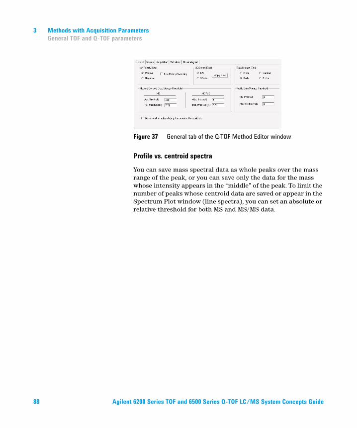
3 Methods with Acquisition Parameters
General TOF and Q-TOF parameters
Profile vs. centroid spectra
You can save mass spectral data as whole peaks over the mass range of the peak, or you can save only the data for the mass whose intensity appears in the “middle” of the peak. To limit the number of peaks whose centroid data are saved or appear in the Spectrum Plot window (line spectra), you can set an absolute or relative threshold for both MS and MS/MS data.
Figure 37 General tab of the Q-TOF Method Editor window
88 Agilent 6200 Series TOF and 6500 Series Q-TOF LC/MS System Concepts Guide
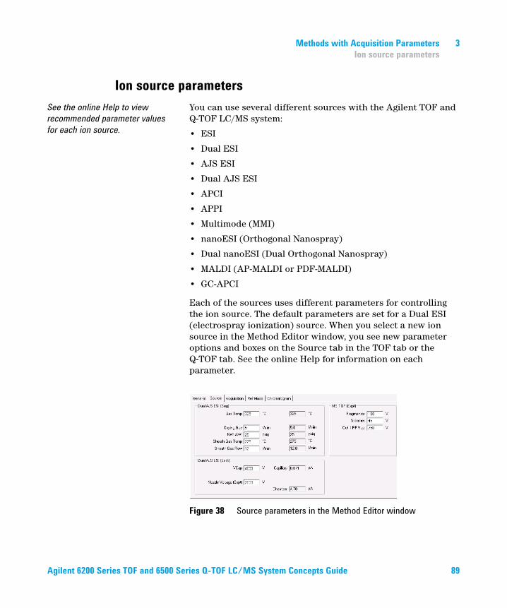
Methods with Acquisition Parameters 3
Ion source parameters
Ion source parameters
See the online Help to view
recommended parameter values
for each ion source.
You can use several different sources with the Agilent TOF and Q-TOF LC/MS system:
• ESI
• Dual ESI
• AJS ESI
• Dual AJS ESI
• APCI
• APPI
• Multimode (MMI)
• nanoESI (Orthogonal Nanospray)
• Dual nanoESI (Dual Orthogonal Nanospray)
• MALDI (AP-MALDI or PDF-MALDI)
• GC-APCI
Each of the sources uses different parameters for controlling the ion source. The default parameters are set for a Dual ESI (electrospray ionization) source. When you select a new ion source in the Method Editor window, you see new parameter options and boxes on the Source tab in the TOF tab or the Q-TOF tab. See the online Help for information on each parameter.
Figure 38 Source parameters in the Method Editor window
Agilent 6200 Series TOF and 6500 Series Q-TOF LC/MS System Concepts Guide 89
3 Methods with Acquisition Parameters
Ion source parameters
Tips for using the AP-MALDI or PDF-MALDI source
For instructions on how to set up
and run samples with the
AP-MALDI and PDF-MALDI inlet
and ion source, see the online
Help.
For instructions on how to install
the AP-MALDI or PDF-MALDI ion
source, see the Installation Guide.
Before the AP-MALDI or the
PDF-MALDI is installed, in the
instrument configuration tool, the
LC must be removed from the
system configuration.
For more information on how to
set up the AP-MALDI to introduce
samples, refer to the Agilent
G1972A AP-MALDI LC/MSD Trap
SL System User Guide.
• Tune the TOF or Q-TOF with an ESI source installed
• Make sure the Run Type in the Sample Run window is set to External Start.
• Set the proper settings in the AP-MALDI or PDF-MALDI control software, and make sure that the desorption time is not less than the MS TOF stop time.
Auto tune for the AP-MALDI and PDF-MALDI source is not supported. You can use Manual Tune to tune the instrument when either of these sources is installed.
90 Agilent 6200 Series TOF and 6500 Series Q-TOF LC/MS System Concepts Guide
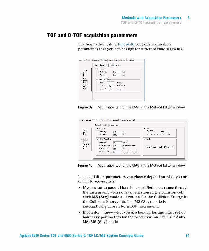
Methods with Acquisition Parameters 3
TOF and Q-TOF acquisition parameters
TOF and Q-TOF acquisition parameters
The Acquisition tab in Figure 40 contains acquisition parameters that you can change for different time segments.
The acquisition parameters you choose depend on what you are trying to accomplish:
• If you want to pass all ions in a specified mass range through the instrument with no fragmentation in the collision cell, click MS (Seg) mode and enter 0 for the Collision Energy in the Collision Energy tab. The MS (Seg) mode is automatically chosen for a TOF instrument.
• If you don't know what you are looking for and must set up boundary parameters for the precursor ion list, click Auto MS/MS (Seg) mode.
Figure 39 Acquisition tab for the 6550 in the Method Editor window
Figure 40 Acquisition tab for the 6560 in the Method Editor window
Agilent 6200 Series TOF and 6500 Series Q-TOF LC/MS System Concepts Guide 91
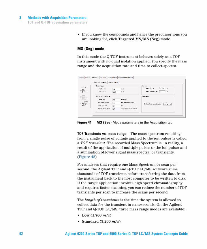
3 Methods with Acquisition Parameters
TOF and Q-TOF acquisition parameters
• If you know the compounds and hence the precursor ions you are looking for, click Targeted MS/MS (Seg) mode.
MS (Seg) mode
In this mode the Q-TOF instrument behaves solely as a TOF instrument with no quad isolation applied. You specify the mass range and the acquisition rate and time to collect spectra.
TOF Transients vs. mass range The mass spectrum resulting from a single pulse of voltage applied to the ion pulser is called a TOF transient. The recorded Mass Spectrum is, in reality, a result of the application of multiple pulses to the ion pulser and a summation of lower signal mass spectra, or transients. (Figure 42)
For analyses that require one Mass Spectrum or scan per second, the Agilent TOF and Q-TOF LC/MS software sums thousands of TOF transients before transferring the data from the instrument back to the host computer to be written to disk. If the target application involves high speed chromatography and requires faster scanning, you can reduce the number of TOF transients per scan to increase the scans per second.
The length of transients is the time the system is allowed to collect data for the transient in nanoseconds. On the Agilent TOF and Q-TOF LC/MS, three mass range modes are available:
• Low (1,700 m/z)
• Standard (3,200 m/z)
Figure 41 MS (Seg) Mode parameters in the Acquisition tab
92 Agilent 6200 Series TOF and 6500 Series Q-TOF LC/MS System Concepts Guide
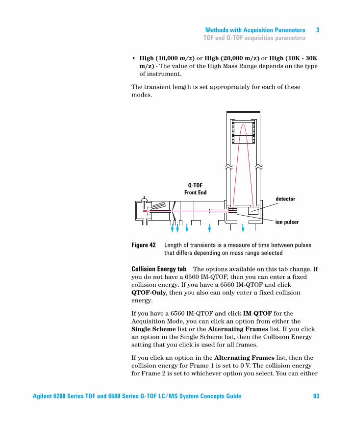
Methods with Acquisition Parameters 3
TOF and Q-TOF acquisition parameters
• High (10,000 m/z) or High (20,000 m/z) or High (10K - 30K m/z) - The value of the High Mass Range depends on the type of instrument.
The transient length is set appropriately for each of these modes.
Figure 42 Length of transients is a measure of time between pulses
that differs depending on mass range selected
Collision Energy tab The options available on this tab change. If you do not have a 6560 IM-QTOF, then you can enter a fixed collision energy. If you have a 6560 IM-QTOF and click QTOF-Only, then you also can only enter a fixed collision energy.
If you have a 6560 IM-QTOF and click IM-QTOF for the Acquisition Mode, you can click an option from either the Single Scheme list or the Alternating Frames list. If you click an option in the Single Scheme list, then the Collision Energy setting that you click is used for all frames.
If you click an option in the Alternating Frames list, then the collision energy for Frame 1 is set to 0 V. The collision energy for Frame 2 is set to whichever option you select. You can either
ion pulser
detector
Q-TOFFront End
Agilent 6200 Series TOF and 6500 Series Q-TOF LC/MS System Concepts Guide 93
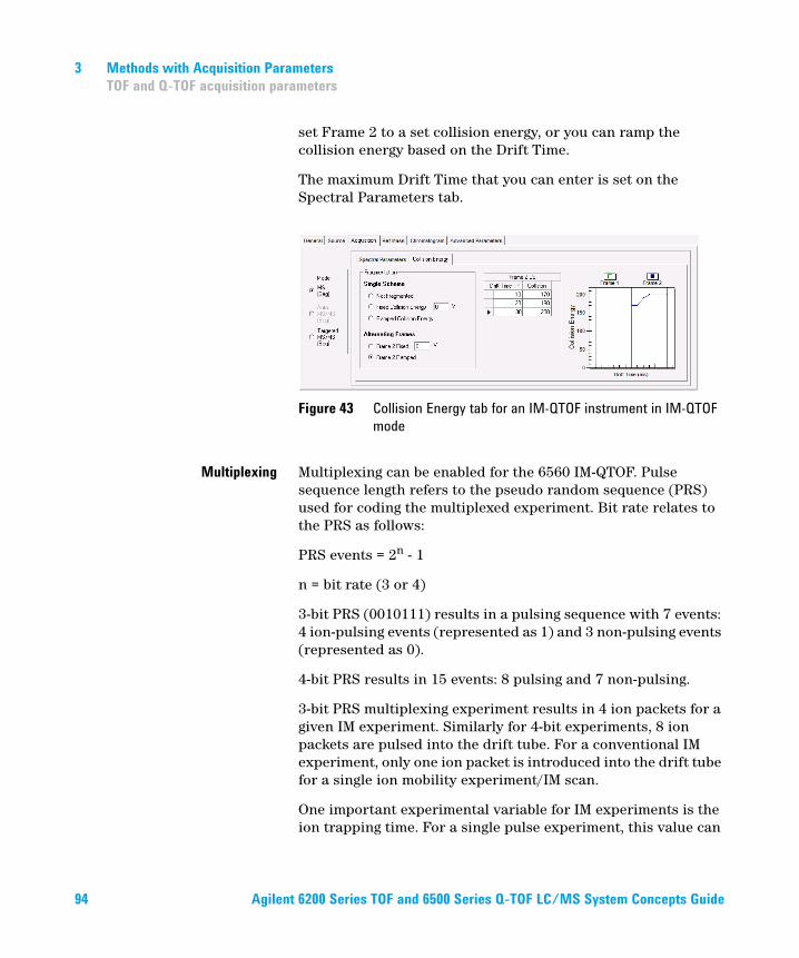
3 Methods with Acquisition Parameters
TOF and Q-TOF acquisition parameters
set Frame 2 to a set collision energy, or you can ramp the collision energy based on the Drift Time.
The maximum Drift Time that you can enter is set on the Spectral Parameters tab.
Multiplexing Multiplexing can be enabled for the 6560 IM-QTOF. Pulse sequence length refers to the pseudo random sequence (PRS) used for coding the multiplexed experiment. Bit rate relates to the PRS as follows:
PRS events = 2n - 1
n = bit rate (3 or 4)
3-bit PRS (0010111) results in a pulsing sequence with 7 events: 4 ion-pulsing events (represented as 1) and 3 non-pulsing events (represented as 0).
4-bit PRS results in 15 events: 8 pulsing and 7 non-pulsing.
3-bit PRS multiplexing experiment results in 4 ion packets for a given IM experiment. Similarly for 4-bit experiments, 8 ion packets are pulsed into the drift tube. For a conventional IM experiment, only one ion packet is introduced into the drift tube for a single ion mobility experiment/IM scan.
One important experimental variable for IM experiments is the ion trapping time. For a single pulse experiment, this value can
Figure 43 Collision Energy tab for an IM-QTOF instrument in IM-QTOF
mode
94 Agilent 6200 Series TOF and 6500 Series Q-TOF LC/MS System Concepts Guide
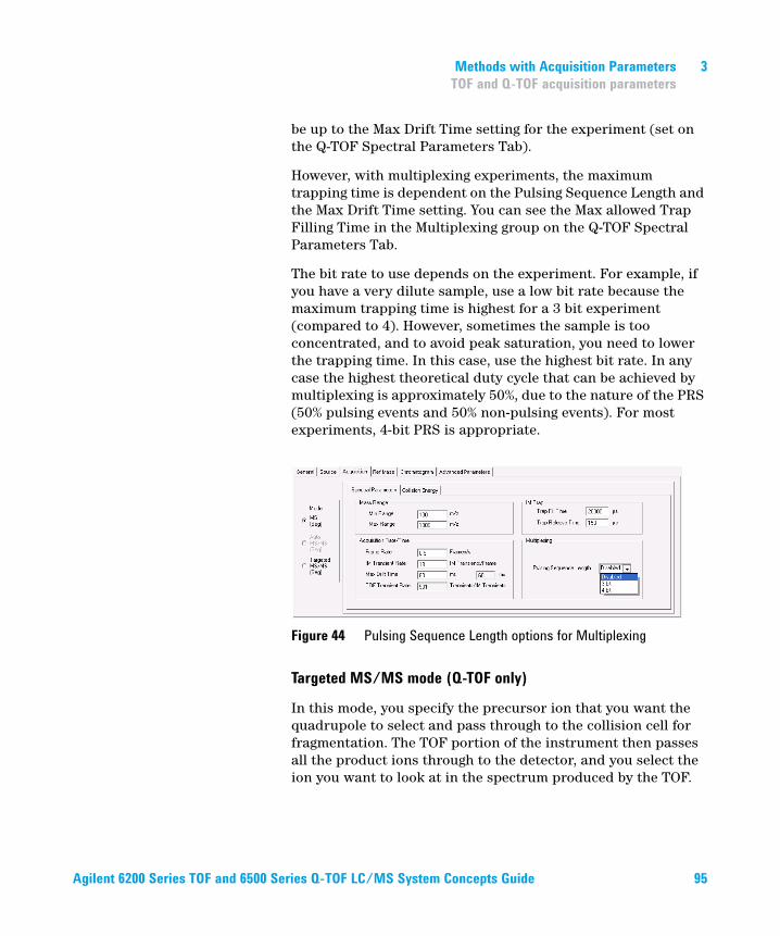
Methods with Acquisition Parameters 3
TOF and Q-TOF acquisition parameters
be up to the Max Drift Time setting for the experiment (set on the Q-TOF Spectral Parameters Tab).
However, with multiplexing experiments, the maximum trapping time is dependent on the Pulsing Sequence Length and the Max Drift Time setting. You can see the Max allowed Trap Filling Time in the Multiplexing group on the Q-TOF Spectral Parameters Tab.
The bit rate to use depends on the experiment. For example, if you have a very dilute sample, use a low bit rate because the maximum trapping time is highest for a 3 bit experiment (compared to 4). However, sometimes the sample is too concentrated, and to avoid peak saturation, you need to lower the trapping time. In this case, use the highest bit rate. In any case the highest theoretical duty cycle that can be achieved by multiplexing is approximately 50%, due to the nature of the PRS (50% pulsing events and 50% non-pulsing events). For most experiments, 4-bit PRS is appropriate.
Targeted MS/MS mode (Q-TOF only)
In this mode, you specify the precursor ion that you want the quadrupole to select and pass through to the collision cell for fragmentation. The TOF portion of the instrument then passes all the product ions through to the detector, and you select the ion you want to look at in the spectrum produced by the TOF.
Figure 44 Pulsing Sequence Length options for Multiplexing
Agilent 6200 Series TOF and 6500 Series Q-TOF LC/MS System Concepts Guide 95
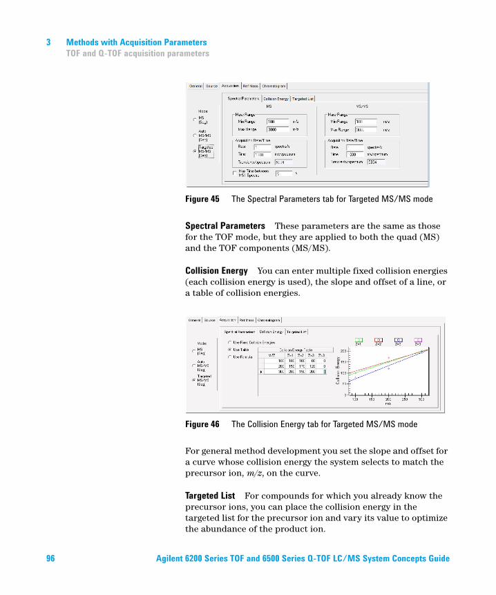
3 Methods with Acquisition Parameters
TOF and Q-TOF acquisition parameters
Spectral Parameters These parameters are the same as those for the TOF mode, but they are applied to both the quad (MS) and the TOF components (MS/MS).
Collision Energy You can enter multiple fixed collision energies (each collision energy is used), the slope and offset of a line, or a table of collision energies.
For general method development you set the slope and offset for a curve whose collision energy the system selects to match the precursor ion, m/z, on the curve.
Targeted List For compounds for which you already know the precursor ions, you can place the collision energy in the targeted list for the precursor ion and vary its value to optimize the abundance of the product ion.
Figure 45 The Spectral Parameters tab for Targeted MS/MS mode
Figure 46 The Collision Energy tab for Targeted MS/MS mode
96 Agilent 6200 Series TOF and 6500 Series Q-TOF LC/MS System Concepts Guide
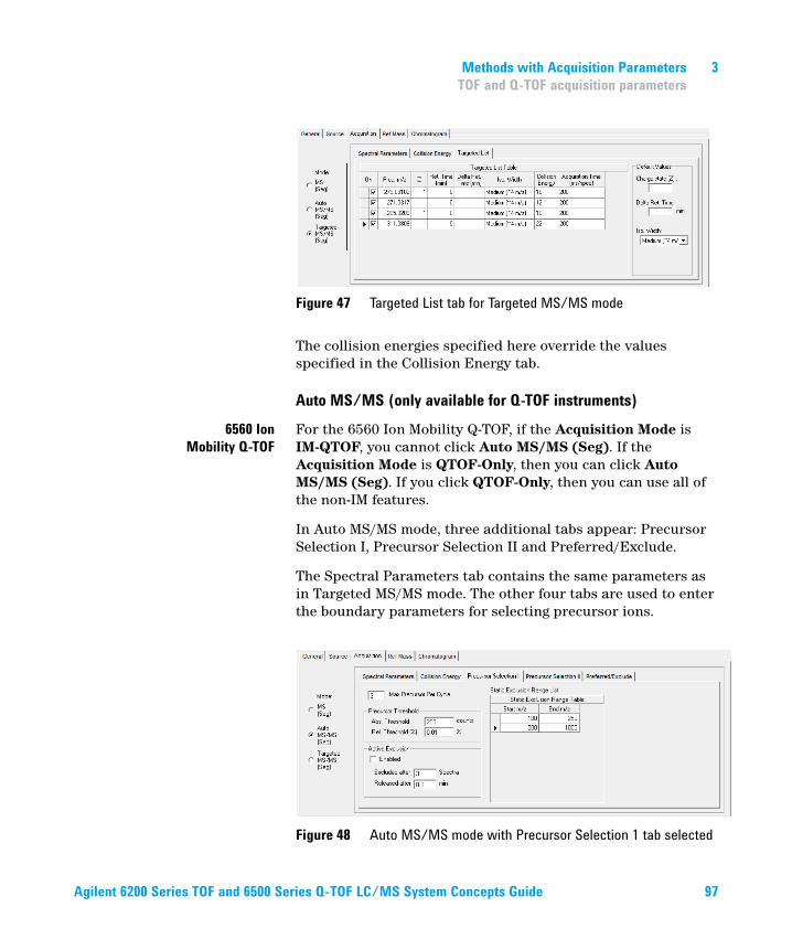
Methods with Acquisition Parameters 3
TOF and Q-TOF acquisition parameters
The collision energies specified here override the values specified in the Collision Energy tab.
Auto MS/MS (only available for Q-TOF instruments)
6560 Ion
Mobility Q-TOF
For the 6560 Ion Mobility Q-TOF, if the Acquisition Mode is IM-QTOF, you cannot click Auto MS/MS (Seg). If the Acquisition Mode is QTOF-Only, then you can click Auto MS/MS (Seg). If you click QTOF-Only, then you can use all of the non-IM features.
In Auto MS/MS mode, three additional tabs appear: Precursor Selection I, Precursor Selection II and Preferred/Exclude.
The Spectral Parameters tab contains the same parameters as in Targeted MS/MS mode. The other four tabs are used to enter the boundary parameters for selecting precursor ions.
Figure 47 Targeted List tab for Targeted MS/MS mode
Figure 48 Auto MS/MS mode with Precursor Selection 1 tab selected
Agilent 6200 Series TOF and 6500 Series Q-TOF LC/MS System Concepts Guide 97
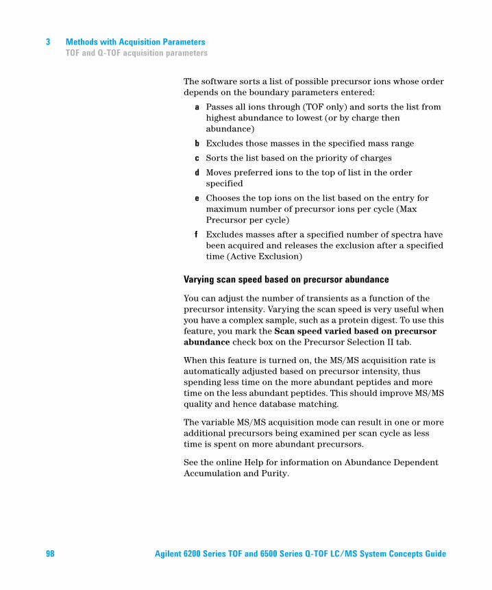
3 Methods with Acquisition Parameters
TOF and Q-TOF acquisition parameters
The software sorts a list of possible precursor ions whose order depends on the boundary parameters entered:
a Passes all ions through (TOF only) and sorts the list from highest abundance to lowest (or by charge then abundance)
b Excludes those masses in the specified mass range
c Sorts the list based on the priority of charges
d Moves preferred ions to the top of list in the order specified
e Chooses the top ions on the list based on the entry for maximum number of precursor ions per cycle (Max Precursor per cycle)
f Excludes masses after a specified number of spectra have been acquired and releases the exclusion after a specified time (Active Exclusion)
Varying scan speed based on precursor abundance
You can adjust the number of transients as a function of the precursor intensity. Varying the scan speed is very useful when you have a complex sample, such as a protein digest. To use this feature, you mark the Scan speed varied based on precursor abundance check box on the Precursor Selection II tab.
When this feature is turned on, the MS/MS acquisition rate is automatically adjusted based on precursor intensity, thus spending less time on the more abundant peptides and more time on the less abundant peptides. This should improve MS/MS quality and hence database matching.
The variable MS/MS acquisition mode can result in one or more additional precursors being examined per scan cycle as less time is spent on more abundant precursors.
See the online Help for information on Abundance Dependent Accumulation and Purity.
98 Agilent 6200 Series TOF and 6500 Series Q-TOF LC/MS System Concepts Guide
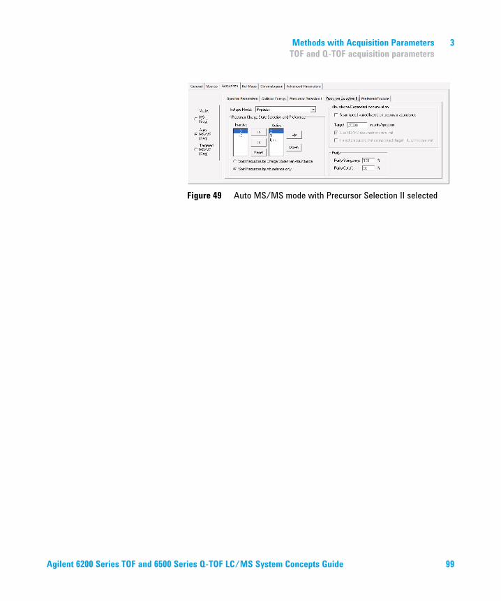
Methods with Acquisition Parameters 3
TOF and Q-TOF acquisition parameters
Figure 49 Auto MS/MS mode with Precursor Selection II selected
Agilent 6200 Series TOF and 6500 Series Q-TOF LC/MS System Concepts Guide 99
3 Methods with Acquisition Parameters
Setup of TOF and Q-TOF reference mass correction (recalibration)
Setup of TOF and Q-TOF reference mass correction (recalibration)
You must do mass corrections
during a run in order to attain the
mass accuracy that Agilent
specifies for the TOF and Q-TOF.
Many applications need as small a deviation of accurate mass as possible. To obtain this accuracy, you recalibrate the mass axis for every spectrum with measurements of known reference masses (i.e “lock masses”). You measure the masses of reference compounds in a reference standard, which can be the Agilent reference standard or one of your own choosing.
If you have an 6560 Ion Mobility Q-TOF, you can only enable reference mass correction if the Acquisition Mode is QTOF-Only. If the Acquisition Mode is IM-QTOF, then you instead can use the IM-MS Data File Reprocessing Utility. See the online Help for the IM-MS Browser program for more information on this utility.
You can introduce the reference standard into the TOF system in one of three ways:
• A calibrant delivery system (CDS) that automatically introduces the standard to a reference sprayer (second sprayer)— Dual ESI (0.2 to 1.5 mL/min flow rates only), Dual AJS ESI and Dual nano ESI
• An external dispense pump—other ion sources
• Addition to the sample—other ion sources
Enabling reference mass correction
You set up and enable reference mass correction in the Ref Mass tab within the TOF tab or the Q-TOF tab of the Method Editor window.
100 Agilent 6200 Series TOF and 6500 Series Q-TOF LC/MS System Concepts Guide
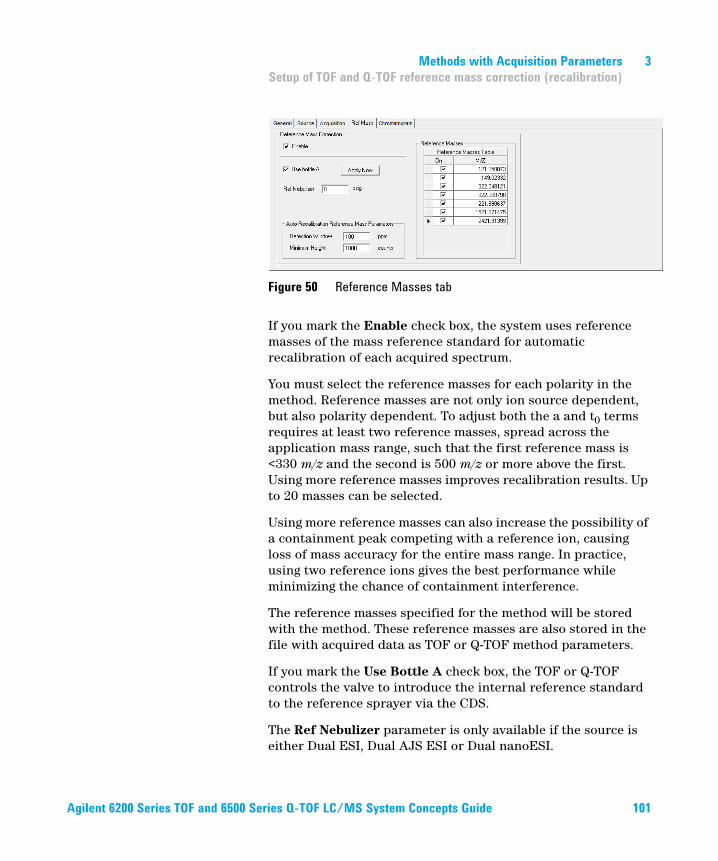
Methods with Acquisition Parameters 3
Setup of TOF and Q-TOF reference mass correction (recalibration)
If you mark the Enable check box, the system uses reference masses of the mass reference standard for automatic recalibration of each acquired spectrum.
You must select the reference masses for each polarity in the method. Reference masses are not only ion source dependent, but also polarity dependent. To adjust both the a and t0 terms requires at least two reference masses, spread across the application mass range, such that the first reference mass is <330 m/z and the second is 500 m/z or more above the first. Using more reference masses improves recalibration results. Up to 20 masses can be selected.
Using more reference masses can also increase the possibility of a containment peak competing with a reference ion, causing loss of mass accuracy for the entire mass range. In practice, using two reference ions gives the best performance while minimizing the chance of containment interference.
The reference masses specified for the method will be stored with the method. These reference masses are also stored in the file with acquired data as TOF or Q-TOF method parameters.
If you mark the Use Bottle A check box, the TOF or Q-TOF controls the valve to introduce the internal reference standard to the reference sprayer via the CDS.
The Ref Nebulizer parameter is only available if the source is either Dual ESI, Dual AJS ESI or Dual nanoESI.
Figure 50 Reference Masses tab
Agilent 6200 Series TOF and 6500 Series Q-TOF LC/MS System Concepts Guide 101
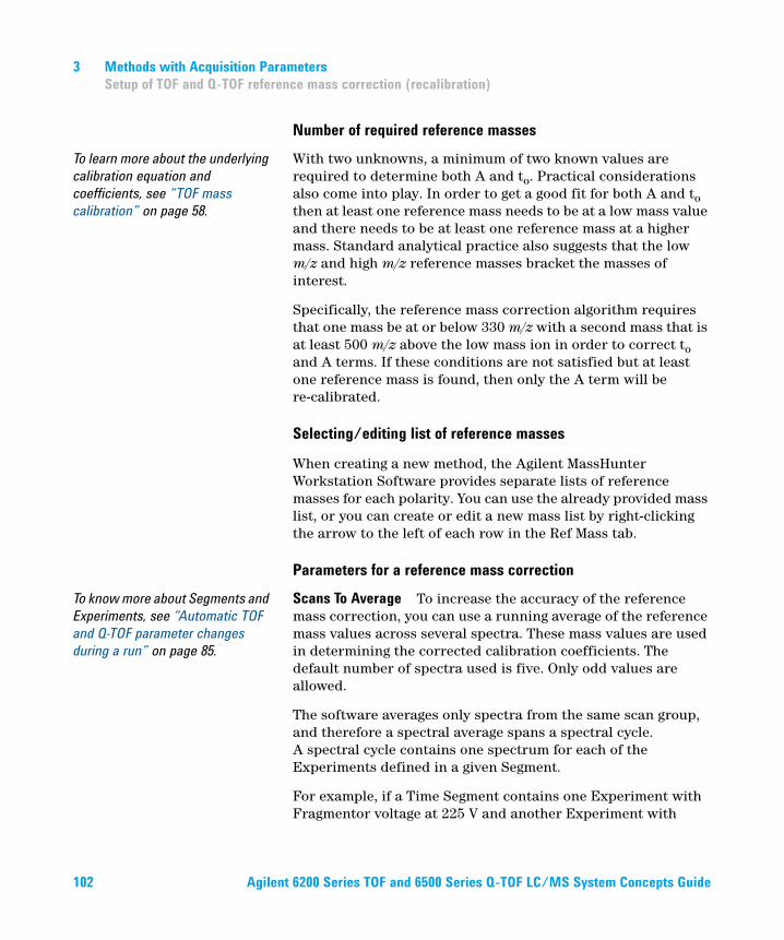
3 Methods with Acquisition Parameters
Setup of TOF and Q-TOF reference mass correction (recalibration)
Number of required reference masses
To learn more about the underlying
calibration equation and
coefficients, see “TOF mass
calibration” on page 58.
With two unknowns, a minimum of two known values are required to determine both A and to. Practical considerations also come into play. In order to get a good fit for both A and to then at least one reference mass needs to be at a low mass value and there needs to be at least one reference mass at a higher mass. Standard analytical practice also suggests that the low m/z and high m/z reference masses bracket the masses of interest.
Specifically, the reference mass correction algorithm requires that one mass be at or below 330 m/z with a second mass that is at least 500 m/z above the low mass ion in order to correct to and A terms. If these conditions are not satisfied but at least one reference mass is found, then only the A term will be re-calibrated.
Selecting/editing list of reference masses
When creating a new method, the Agilent MassHunter Workstation Software provides separate lists of reference masses for each polarity. You can use the already provided mass list, or you can create or edit a new mass list by right-clicking the arrow to the left of each row in the Ref Mass tab.
Parameters for a reference mass correction
To know more about Segments and
Experiments, see “Automatic TOF
and Q-TOF parameter changes
during a run” on page 85.
Scans To Average To increase the accuracy of the reference mass correction, you can use a running average of the reference mass values across several spectra. These mass values are used in determining the corrected calibration coefficients. The default number of spectra used is five. Only odd values are allowed.
The software averages only spectra from the same scan group, and therefore a spectral average spans a spectral cycle. A spectral cycle contains one spectrum for each of the Experiments defined in a given Segment.
For example, if a Time Segment contains one Experiment with Fragmentor voltage at 225 V and another Experiment with
102 Agilent 6200 Series TOF and 6500 Series Q-TOF LC/MS System Concepts Guide
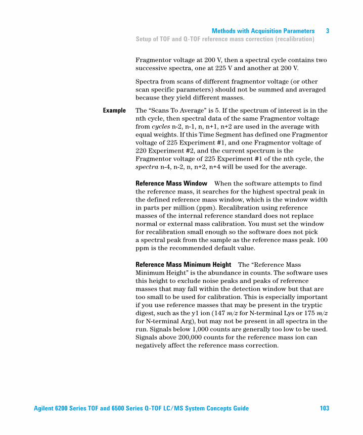
Methods with Acquisition Parameters 3
Setup of TOF and Q-TOF reference mass correction (recalibration)
Fragmentor voltage at 200 V, then a spectral cycle contains two successive spectra, one at 225 V and another at 200 V.
Spectra from scans of different fragmentor voltage (or other scan specific parameters) should not be summed and averaged because they yield different masses.
Example The “Scans To Average” is 5. If the spectrum of interest is in the nth cycle, then spectral data of the same Fragmentor voltage from cycles n-2, n-1, n, n+1, n+2 are used in the average with equal weights. If this Time Segment has defined one Fragmentor voltage of 225 Experiment #1, and one Fragmentor voltage of 220 Experiment #2, and the current spectrum is the Fragmentor voltage of 225 Experiment #1 of the nth cycle, the spectra n-4, n-2, n, n+2, n+4 will be used for the average.
Reference Mass Window When the software attempts to find the reference mass, it searches for the highest spectral peak in the defined reference mass window, which is the window width in parts per million (ppm). Recalibration using reference masses of the internal reference standard does not replace normal or external mass calibration. You must set the window for recalibration small enough so the software does not pick a spectral peak from the sample as the reference mass peak. 100 ppm is the recommended default value.
Reference Mass Minimum Height The “Reference Mass Minimum Height” is the abundance in counts. The software uses this height to exclude noise peaks and peaks of reference masses that may fall within the detection window but that are too small to be used for calibration. This is especially important if you use reference masses that may be present in the tryptic digest, such as the y1 ion (147 m/z for N-terminal Lys or 175 m/z for N-terminal Arg), but may not be present in all spectra in the run. Signals below 1,000 counts are generally too low to be used. Signals above 200,000 counts for the reference mass ion can negatively affect the reference mass correction.
Agilent 6200 Series TOF and 6500 Series Q-TOF LC/MS System Concepts Guide 103
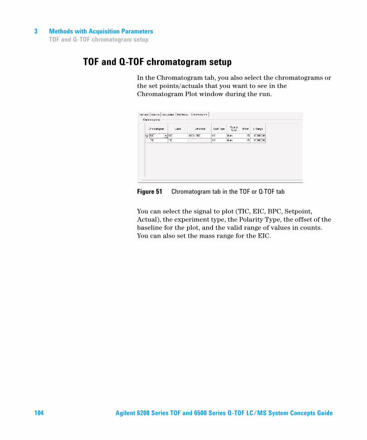
3 Methods with Acquisition Parameters
TOF and Q-TOF chromatogram setup
TOF and Q-TOF chromatogram setup
In the Chromatogram tab, you also select the chromatograms or the set points/actuals that you want to see in the Chromatogram Plot window during the run.
You can select the signal to plot (TIC, EIC, BPC, Setpoint, Actual), the experiment type, the Polarity Type, the offset of the baseline for the plot, and the valid range of values in counts. You can also set the mass range for the EIC.
Figure 51 Chromatogram tab in the TOF or Q-TOF tab
104 Agilent 6200 Series TOF and 6500 Series Q-TOF LC/MS System Concepts Guide
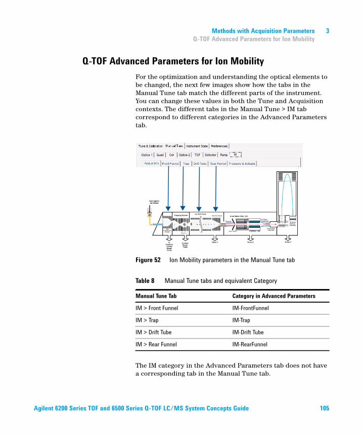
Methods with Acquisition Parameters 3
Q-TOF Advanced Parameters for Ion Mobility
Q-TOF Advanced Parameters for Ion Mobility
For the optimization and understanding the optical elements to be changed, the next few images show how the tabs in the Manual Tune tab match the different parts of the instrument. You can change these values in both the Tune and Acquisition contexts. The different tabs in the Manual Tune > IM tab correspond to different categories in the Advanced Parameters tab.
The IM category in the Advanced Parameters tab does not have a corresponding tab in the Manual Tune tab.
Figure 52 Ion Mobility parameters in the Manual Tune tab
Table 8 Manual Tune tabs and equivalent Category
Manual Tune Tab Category in Advanced Parameters
IM > Front Funnel IM-FrontFunnel
IM > Trap IM-Trap
IM > Drift Tube IM-Drift Tube
IM > Rear Funnel IM-RearFunnel
Agilent 6200 Series TOF and 6500 Series Q-TOF LC/MS System Concepts Guide 105
3 Methods with Acquisition Parameters
Q-TOF Advanced Parameters for Ion Mobility
IM-Front
Funnel
The Trap Funnel RF is the most critical parameter for all applications, as a too low value leads to defocused ions, resulting in a loss in sensitivity. A value that is too high can lead to excessive ion-heating, resulting in fragmentation of labile molecules, or structural changes of molecules. A minor effect is observed from the High Pressure Funnel RF; a lower value is typically used for small and labile compounds.
IM Trap Trap grids low are the values when pulsing the ions out of the trap. These values are the values when operating the instrument in Q-TOF mode. Usually the exit grids do not need any further adjustment from the autotune delivered with the instrument. The high voltages (gray) are the sums of the grid delta (top values) and the low values; these are the actual applied voltages during trapping. Trap Exit Grid 2 Delta needs to be reduced for small molecules and increased for large molecules. In some cases, it might be advantageous to decrease the total DC field in the trap by further reducing the delta between Trap Exit and Trap Entrance (to as low as 0.5V) combined with lowering the Trap Entrance Grid Low.
IM Drift Tube This is calculated as the effective field ((Drift Tube Entrance Voltage minus Drift Tube Exit Voltage) divided by drift tube length). For accurate determination of collision cross sections, this voltage needs to be changed stepwise. See the Familiarization Guide for more information.
IM Rear Funnel For IM Rear Funnel parameters, the RF need to be reduced for labile molecules. Depending on the total decrease, a drop in IM-MS resolution might occur and will be part of the individual compound optimization. In general, a delta of 2V between the Rear Funnel Exit and IM Hex Entrance should be maintained for almost all applications. The absolute potential value of IM Hex Entrance is determined by the Octopole Entrance Lens and IM Hex Delta voltages; it should be another 1 to 2V delta between IM Hex Exit (not a directly editable parameter) and Octopole Entrance Lens.
106 Agilent 6200 Series TOF and 6500 Series Q-TOF LC/MS System Concepts Guide
Methods with Acquisition Parameters 3
Q-TOF Advanced Parameters for Ion Mobility
All IM-MS parameters described in the Tune window are accessible in the Advanced Parameters tab of the Q-TOF tab. The table contains a Use Method column. If you mark this column, then the value you specify is used instead of the value in the tune file. Different samples require different parameters to be changed from the tune file.
Agilent 6200 Series TOF and 6500 Series Q-TOF LC/MS System Concepts Guide 107
3 Methods with Acquisition Parameters
Setting parameters to acquire a data file in All Ions MS/MS mode
Setting parameters to acquire a data file in All Ions MS/MS mode
In order to acquire a data file in All Ions MS/MS mode, you need to set up a method that has a Time Segment with at least two and a maximum of four different Experiments containing different Collision Energy values on a Q-TOF or different Fragmentor voltages on a TOF.
To set up All Ions MS/MS mode when you have an 6560 IM-QTOF, see “Setting parameters on a 6560 IM-QTOF to acquire a data file in All Ions MS/MS mode” on page 111.
The low energy Experiment provides MS information, and the high energy Experiments provide MS/MS fragment information. See the Qualitative Analysis Familiarization Guide for LC/MS for more information on analyzing a data file that was acquired in All Ions mode.
If you have a Q-TOF instrument, you set the Collision Energy to 0 in the first Experiment. In the subsequent Experiments (channels), you set the Collision Energy to a higher value (for example, 20 V). If you are creating a method for a Q-TOF with different collision energies, you set the Fragmentor voltage at the same value in each experiment. It should be set to a low enough setting that no fragments are generated in the source but at a high enough setting that you get enough precursor ions transmitted to the skimmer. This value depends on the compounds you are analyzing and their stability.You set the Collision Energy on the Acquisition > Collision Energy tab and the Fragmentor voltage on the Source tab.
108 Agilent 6200 Series TOF and 6500 Series Q-TOF LC/MS System Concepts Guide
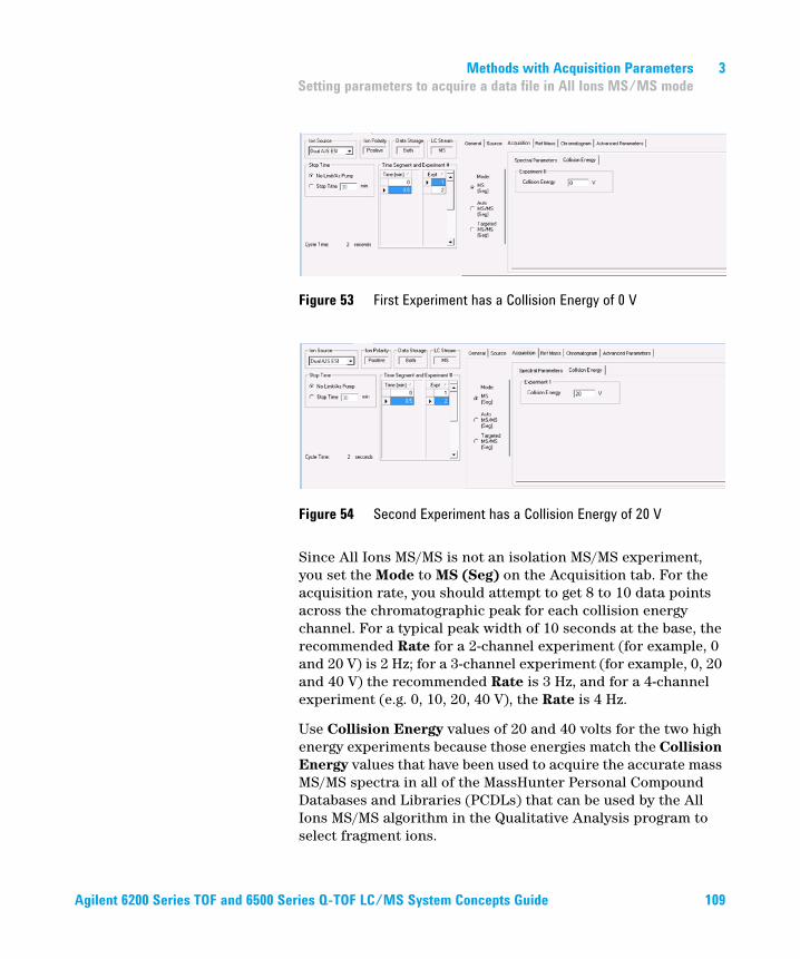
Methods with Acquisition Parameters 3
Setting parameters to acquire a data file in All Ions MS/MS mode
Since All Ions MS/MS is not an isolation MS/MS experiment, you set the Mode to MS (Seg) on the Acquisition tab. For the acquisition rate, you should attempt to get 8 to 10 data points across the chromatographic peak for each collision energy channel. For a typical peak width of 10 seconds at the base, the recommended Rate for a 2-channel experiment (for example, 0 and 20 V) is 2 Hz; for a 3-channel experiment (for example, 0, 20 and 40 V) the recommended Rate is 3 Hz, and for a 4-channel experiment (e.g. 0, 10, 20, 40 V), the Rate is 4 Hz.
Use Collision Energy values of 20 and 40 volts for the two high energy experiments because those energies match the Collision Energy values that have been used to acquire the accurate mass MS/MS spectra in all of the MassHunter Personal Compound Databases and Libraries (PCDLs) that can be used by the All Ions MS/MS algorithm in the Qualitative Analysis program to select fragment ions.
Figure 53 First Experiment has a Collision Energy of 0 V
Figure 54 Second Experiment has a Collision Energy of 20 V
Agilent 6200 Series TOF and 6500 Series Q-TOF LC/MS System Concepts Guide 109
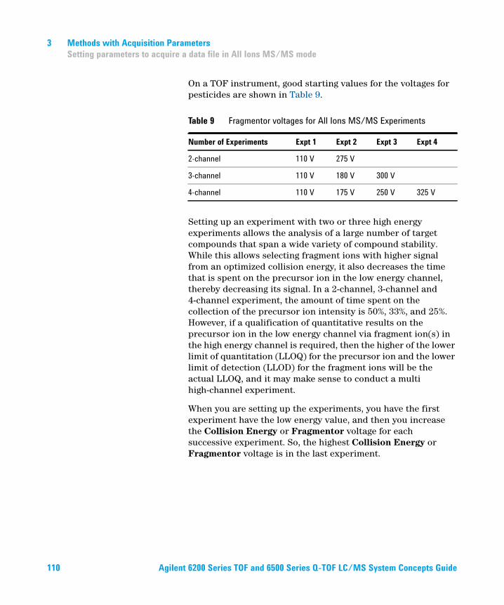
3 Methods with Acquisition Parameters
Setting parameters to acquire a data file in All Ions MS/MS mode
On a TOF instrument, good starting values for the voltages for pesticides are shown in Table 9.
Setting up an experiment with two or three high energy experiments allows the analysis of a large number of target compounds that span a wide variety of compound stability. While this allows selecting fragment ions with higher signal from an optimized collision energy, it also decreases the time that is spent on the precursor ion in the low energy channel, thereby decreasing its signal. In a 2-channel, 3-channel and 4-channel experiment, the amount of time spent on the collection of the precursor ion intensity is 50%, 33%, and 25%. However, if a qualification of quantitative results on the precursor ion in the low energy channel via fragment ion(s) in the high energy channel is required, then the higher of the lower limit of quantitation (LLOQ) for the precursor ion and the lower limit of detection (LLOD) for the fragment ions will be the actual LLOQ, and it may make sense to conduct a multi high-channel experiment.
When you are setting up the experiments, you have the first experiment have the low energy value, and then you increase the Collision Energy or Fragmentor voltage for each successive experiment. So, the highest Collision Energy or Fragmentor voltage is in the last experiment.
Table 9 Fragmentor voltages for All Ions MS/MS Experiments
Number of Experiments Expt 1 Expt 2 Expt 3 Expt 4
2-channel 110 V 275 V
3-channel 110 V 180 V 300 V
4-channel 110 V 175 V 250 V 325 V
110 Agilent 6200 Series TOF and 6500 Series Q-TOF LC/MS System Concepts Guide
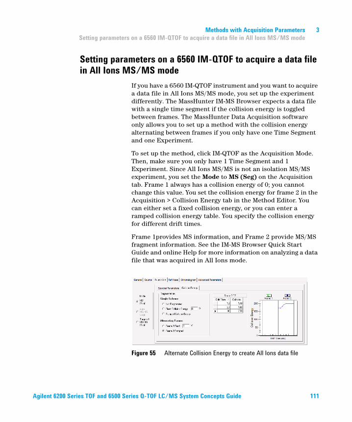
Methods with Acquisition Parameters 3
Setting parameters on a 6560 IM-QTOF to acquire a data file in All Ions MS/MS mode
Setting parameters on a 6560 IM-QTOF to acquire a data file in All Ions MS/MS mode
If you have a 6560 IM-QTOF instrument and you want to acquire a data file in All Ions MS/MS mode, you set up the experiment differently. The MassHunter IM-MS Browser expects a data file with a single time segment if the collision energy is toggled between frames. The MassHunter Data Acquisition software only allows you to set up a method with the collision energy alternating between frames if you only have one Time Segment and one Experiment.
To set up the method, click IM-QTOF as the Acquisition Mode. Then, make sure you only have 1 Time Segment and 1 Experiment. Since All Ions MS/MS is not an isolation MS/MS experiment, you set the Mode to MS (Seg) on the Acquisition tab. Frame 1 always has a collision energy of 0; you cannot change this value. You set the collision energy for frame 2 in the Acquisition > Collision Energy tab in the Method Editor. You can either set a fixed collision energy, or you can enter a ramped collision energy table. You specify the collision energy for different drift times.
Frame 1provides MS information, and Frame 2 provide MS/MS fragment information. See the IM-MS Browser Quick Start Guide and online Help for more information on analyzing a data file that was acquired in All Ions mode.
Figure 55 Alternate Collision Energy to create All Ions data file
Agilent 6200 Series TOF and 6500 Series Q-TOF LC/MS System Concepts Guide 111
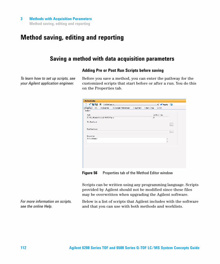
3 Methods with Acquisition Parameters
Method saving, editing and reporting
Method saving, editing and reporting
Saving a method with data acquisition parameters
Adding Pre or Post Run Scripts before saving
To learn how to set up scripts, see
your Agilent application engineer.
Before you save a method, you can enter the pathway for the customized scripts that start before or after a run. You do this on the Properties tab.
Scripts can be written using any programming language. Scripts provided by Agilent should not be modified since these files may be overwritten when upgrading the Agilent software.
For more information on scripts,
see the online Help.
Below is a list of scripts that Agilent includes with the software and that you can use with both methods and worklists.
Figure 56 Properties tab of the Method Editor window
112 Agilent 6200 Series TOF and 6500 Series Q-TOF LC/MS System Concepts Guide
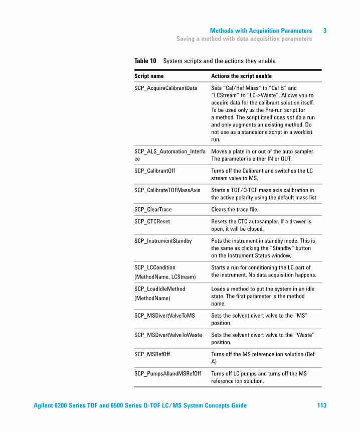
Methods with Acquisition Parameters 3
Saving a method with data acquisition parameters
Table 10 System scripts and the actions they enable
Script name Actions the script enable
SCP_AcquireCalibrantData Sets “Cal/Ref Mass” to “Cal B” and
“LCStream” to “LC->Waste”. Allows you to
acquire data for the calibrant solution itself.
To be used only as the Pre-run script for
a method. The script itself does not do a run
and only augments an existing method. Do
not use as a standalone script in a worklist
run.
SCP_ALS_Automation_Interfa
ce
Moves a plate in or out of the auto sampler.
The parameter is either IN or OUT.
SCP_CalibrantOff Turns off the Calibrant and switches the LC
stream valve to MS.
SCP_CalibrateTOFMassAxis Starts a TOF/Q-TOF mass axis calibration in
the active polarity using the default mass list
SCP_ClearTrace Clears the trace file.
SCP_CTCReset Resets the CTC autosampler. If a drawer is
open, it will be closed.
SCP_InstrumentStandby Puts the instrument in standby mode. This is
the same as clicking the “Standby” button
on the Instrument Status window.
SCP_LCCondition
(MethodName, LCStream)
Starts a run for conditioning the LC part of
the instrument. No data acquisition happens.
SCP_LoadIdleMethod
(MethodName)
Loads a method to put the system in an idle
state. The first parameter is the method
name.
SCP_MSDivertValveToMS Sets the solvent divert valve to the “MS”
position.
SCP_MSDivertValveToWaste Sets the solvent divert valve to the “Waste”
position.
SCP_MSRefOff Turns off the MS reference ion solution (Ref
A)
SCP_PumpsAllandMSRefOff Turns off LC pumps and turns off the MS
reference ion solution.
Agilent 6200 Series TOF and 6500 Series Q-TOF LC/MS System Concepts Guide 113
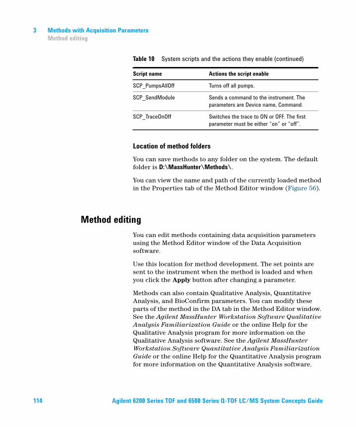
3 Methods with Acquisition Parameters
Method editing
Location of method folders
You can save methods to any folder on the system. The default folder is D:\MassHunter\Methods\.
You can view the name and path of the currently loaded method in the Properties tab of the Method Editor window (Figure 56).
Method editing
You can edit methods containing data acquisition parameters using the Method Editor window of the Data Acquisition software.
Use this location for method development. The set points are sent to the instrument when the method is loaded and when you click the Apply button after changing a parameter.
Methods can also contain Qualitative Analysis, Quantitative Analysis, and BioConfirm parameters. You can modify these parts of the method in the DA tab in the Method Editor window. See the Agilent MassHunter Workstation Software Qualitative Analysis Familiarization Guide or the online Help for the Qualitative Analysis program for more information on the Qualitative Analysis software. See the Agilent MassHunter Workstation Software Quantitative Analysis Familiarization Guide or the online Help for the Quantitative Analysis program for more information on the Quantitative Analysis software.
SCP_PumpsAllOff Turns off all pumps.
SCP_SendModule Sends a command to the instrument. The
parameters are Device name, Command.
SCP_TraceOnOff Switches the trace to ON or OFF. The first
parameter must be either “on” or “off”.
Table 10 System scripts and the actions they enable (continued)
Script name Actions the script enable
114 Agilent 6200 Series TOF and 6500 Series Q-TOF LC/MS System Concepts Guide
Methods with Acquisition Parameters 3
Method reporting
Method reporting
You can see the parameters in a method in one of three ways:
• You click Method Report from the File > Print menu.
• You review the parameters in the Method Editor.
• You can see method parameters associated with a data file in the Agilent MassHunter Workstation Qualitative Analysis software.
Acquisition Method reports include this information:
• Method name, path and description
• List of configured LC modules and TOF or Q-TOF
• Parameter values for the marked devices in the Acquisition Method Report Options dialog box
Agilent 6200 Series TOF and 6500 Series Q-TOF LC/MS System Concepts Guide 115

116 Agilent 6200 Series TOF and 6500 Series Q-TOF LC/MS System Concepts Guide
This page intentionally left blank.
Agilent 6200 Series TOF and 6500 Series Q-TOF LC/MS System
4Data Acquisition
Interactive single sample setup 118
Worklist setup 120
Data acquisition for samples and worklists 136
Learn the concepts to help you understand the setup of single samples for interactive data acquisition and the setup of single samples and sequences of samples for automatic data acquisition.
117
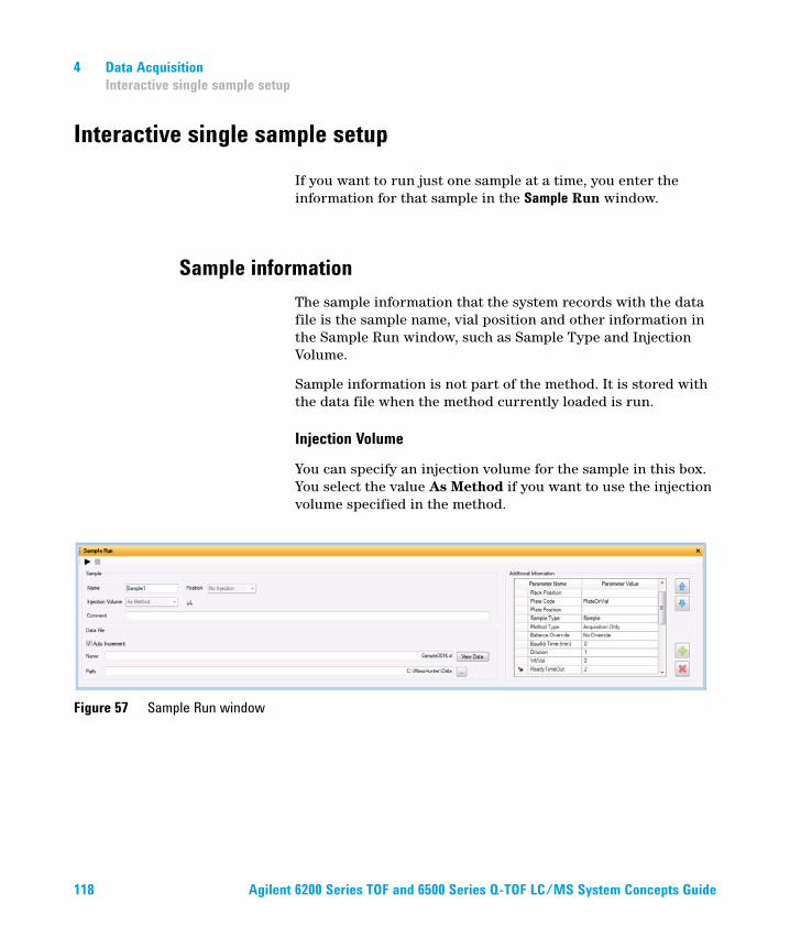
4 Data Acquisition
Interactive single sample setup
Interactive single sample setup
If you want to run just one sample at a time, you enter the information for that sample in the Sample Run window.
Sample information
The sample information that the system records with the data file is the sample name, vial position and other information in the Sample Run window, such as Sample Type and Injection Volume.
Sample information is not part of the method. It is stored with the data file when the method currently loaded is run.
Injection Volume
You can specify an injection volume for the sample in this box. You select the value As Method if you want to use the injection volume specified in the method.
Figure 57 Sample Run window
118 Agilent 6200 Series TOF and 6500 Series Q-TOF LC/MS System Concepts Guide
Data Acquisition 4
Data File information
Data File information
The default folder for TOF/Q-TOF data is D:\MassHunter\Data.
Auto Increment If you want to use the same file name and have the system automatically change the number at the end of the file name, you turn auto-increment on. Then, you type a file name that ends in the number 001, and the system makes sure that a new file is created every time you re-run that sample.
Other folders
You can save your data to any folder on the system. You must use the browse button to select a different folder. To open any data file saved to a different folder than D:\MassHunter\Data,
you must browse to the different folder.
Some of the Additional Information parameters
Sample Type
You specify one of the following types for a single sample run: Sample, Calibration, QC, Blank, DoubleBlank, Matrix, MatrixDup, MatrixBlank, ConCal, TuneCheck, and ResponseCheck.
Method Type
Acquisition Only, DA Only, or Both Acquisition and DA.
Run Types
This value is not shown by default. You can add it by clicking the + button and adding it using the Add Parameters dialog box.
Standard Start for LC runs
Manual Run for infusion runs with a syringe pump
External Start for AP-MALDI
LC Only Run for when you do not acquire MS data
Agilent 6200 Series TOF and 6500 Series Q-TOF LC/MS System Concepts Guide 119
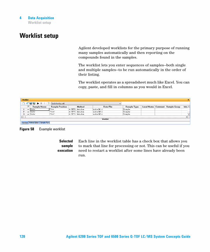
4 Data Acquisition
Worklist setup
Worklist setup
Agilent developed worklists for the primary purpose of running many samples automatically and then reporting on the compounds found in the samples.
The worklist lets you enter sequences of samples—both single and multiple samples—to be run automatically in the order of their listing.
The worklist operates as a spreadsheet much like Excel. You can copy, paste, and fill in columns as you would in Excel.
Selected
sample
execution
Each line in the worklist table has a check box that allows you to mark that line for processing or not. This can be useful if you need to restart a worklist after some lines have already been run.
Figure 58 Example worklist
120 Agilent 6200 Series TOF and 6500 Series Q-TOF LC/MS System Concepts Guide
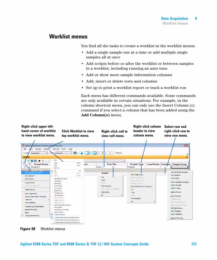
Data Acquisition 4
Worklist menus
Worklist menus
You find all the tasks to create a worklist in the worklist menus.
• Add a single sample one at a time or add multiple single samples all at once
• Add scripts before or after the worklist or between samples in a worklist, including running an auto tune
• Add or show more sample information columns
• Add, insert or delete rows and columns
• Set up to print a worklist report or track a worklist run
Each menu has different commands available. Some commands are only available in certain situations. For example, in the column shortcut menu, you can only use the Insert Column (s) command if you select a column that has been added using the Add Column(s) menu.
Figure 59 Worklist menus
Right-click upper left-
hand corner of worklist
to view worklist menu.Click Worklist to view
top worklist menu.Right-click cell to
view cell menu.
Right-click column
header to view
column menu.
Select row and
right-click row to
view row menu.
Agilent 6200 Series TOF and 6500 Series Q-TOF LC/MS System Concepts Guide 121
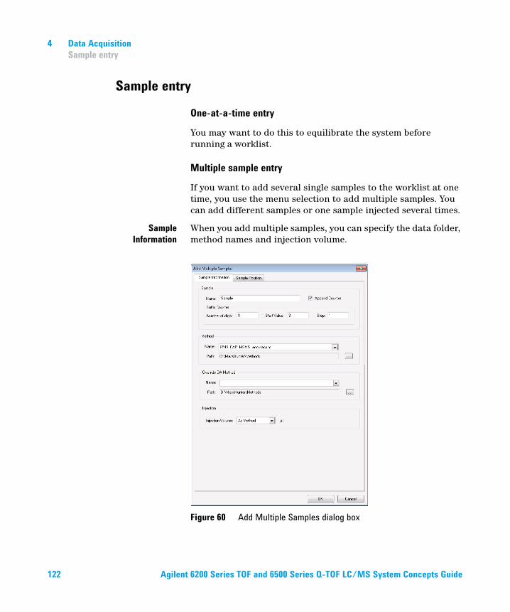
4 Data Acquisition
Sample entry
Sample entry
One-at-a-time entry
You may want to do this to equilibrate the system before running a worklist.
Multiple sample entry
If you want to add several single samples to the worklist at one time, you use the menu selection to add multiple samples. You can add different samples or one sample injected several times.
Sample
Information
When you add multiple samples, you can specify the data folder, method names and injection volume.
Figure 60 Add Multiple Samples dialog box
122 Agilent 6200 Series TOF and 6500 Series Q-TOF LC/MS System Concepts Guide
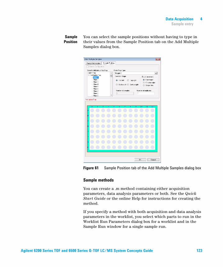
Data Acquisition 4
Sample entry
Sample
Position
You can select the sample positions without having to type in their values from the Sample Position tab on the Add Multiple Samples dialog box.
Sample methods
You can create a .m method containing either acquisition parameters, data analysis parameters or both. See the Quick Start Guide or the online Help for instructions for creating the method.
If you specify a method with both acquisition and data analysis parameters in the worklist, you select which parts to run in the Worklist Run Parameters dialog box for a worklist and in the Sample Run window for a single sample run.
Figure 61 Sample Position tab of the Add Multiple Samples dialog box
Agilent 6200 Series TOF and 6500 Series Q-TOF LC/MS System Concepts Guide 123
4 Data Acquisition
Script entry
Script entry
Scripts are special programs, that
execute automatically. Agilent
includes scripts with the Agilent
MassHunter Workstation
Software, and you can write your
own scripts.
You can enter scripts to be run at the following times:
• Before or after samples as part of the method
The sample method can include pre- and post-analysis scripts. (See Chapter 3, Acquisition Methods)
• Before or after samples in the worklist or batch (insert or add scripts, respectively)
• Before or after a worklist and after data acquisition (Figure 66 on page 131)
Scripts provided by Agilent should not be modified since these files may be overwritten when upgrading the Agilent software.
For detailed instructions on how to enter scripts, see the online Help. For instructions on how to create scripts, see your Agilent application engineer.
Agilent includes scripts with the software to help you automatically, instead of manually, execute processes such as column conditioning and valve shutoff. See Table 10 on page 113 for a list of possible scripts.
124 Agilent 6200 Series TOF and 6500 Series Q-TOF LC/MS System Concepts Guide
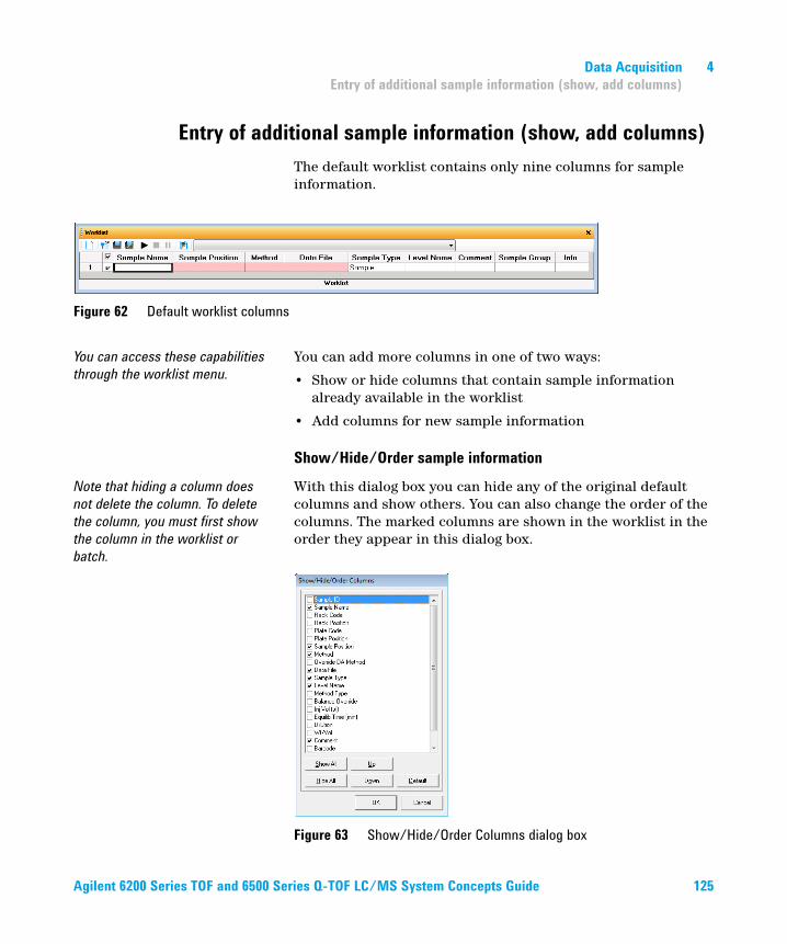
Data Acquisition 4
Entry of additional sample information (show, add columns)
Entry of additional sample information (show, add columns)
The default worklist contains only nine columns for sample information.
You can access these capabilities
through the worklist menu.
You can add more columns in one of two ways:
• Show or hide columns that contain sample information already available in the worklist
• Add columns for new sample information
Show/Hide/Order sample information
Note that hiding a column does
not delete the column. To delete
the column, you must first show
the column in the worklist or
batch.
With this dialog box you can hide any of the original default columns and show others. You can also change the order of the columns. The marked columns are shown in the worklist in the order they appear in this dialog box.
Figure 63 Show/Hide/Order Columns dialog box
Figure 62 Default worklist columns
Agilent 6200 Series TOF and 6500 Series Q-TOF LC/MS System Concepts Guide 125
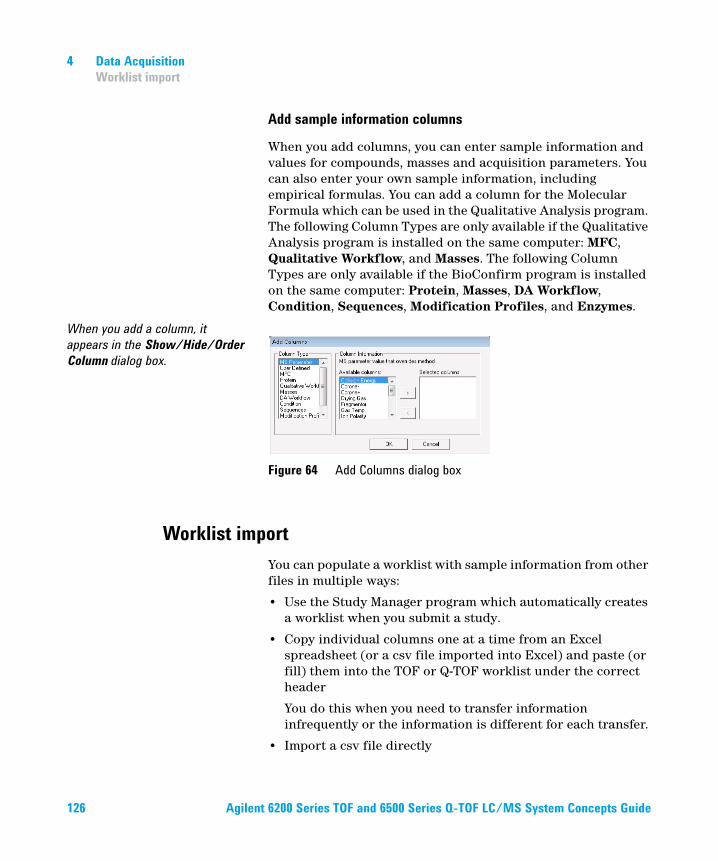
4 Data Acquisition
Worklist import
Add sample information columns
When you add columns, you can enter sample information and values for compounds, masses and acquisition parameters. You can also enter your own sample information, including empirical formulas. You can add a column for the Molecular Formula which can be used in the Qualitative Analysis program. The following Column Types are only available if the Qualitative Analysis program is installed on the same computer: MFC, Qualitative Workflow, and Masses. The following Column Types are only available if the BioConfirm program is installed on the same computer: Protein, Masses, DA Workflow, Condition, Sequences, Modification Profiles, and Enzymes.
When you add a column, it
appears in the Show/Hide/Order Column dialog box.
Worklist import
You can populate a worklist with sample information from other files in multiple ways:
• Use the Study Manager program which automatically creates a worklist when you submit a study.
• Copy individual columns one at a time from an Excel spreadsheet (or a csv file imported into Excel) and paste (or fill) them into the TOF or Q-TOF worklist under the correct header
You do this when you need to transfer information infrequently or the information is different for each transfer.
• Import a csv file directly
Figure 64 Add Columns dialog box
126 Agilent 6200 Series TOF and 6500 Series Q-TOF LC/MS System Concepts Guide
Data Acquisition 4
Worklist import
You cannot import a partial list of
the samples within the csv file.
You do this when you need to use the same parameters in a worklist frequently.
CSV file mapping
You use the Map File Generator program to modify a map file. You start this program by clicking the Map File Generator icon in the Agilent MassHunter Workstation > Acq Tools folder. See the online Help for more information on this program.
You can import the csv file to add
or insert samples whether the
worklist is running or not. You can
also import the file in an offline
session.
Your sample csv file contains a table of samples and attribute information for each sample. The information in this file may not correspond to the information needed in a TOF or Q-TOF worklist in several ways.
• Some of the information may not be relevant.
• Some information may be missing.
• Column names of the sample attributes may not be the same as those used by the Agilent MassHunter Workstation Data Acquisition software.
You cannot import scripts into a
worklist. You must add them
directly.
You must first edit the sample csv file to put it into a form that maps to TOF or Q-TOF sample data. You can specify these changes when you map to the TOF or Q-TOF data:
• Change the column header names
• Add new columns in the worklist
• Change data values
You can include a mapping section in front of the sample information in the sample csv file or in a separate configuration csv file. You use a configuration csv file when all the sample information values are the same from import to import. You also include the mapping section in the sample csv file when new groups of samples with different dynamic mapping of columns, such as amount of compounds analyzed, are added for import.
Mapping for static worklist columns
Some worklist boxes are static and invariant, such as Sample Name and Sample Position. These come under the heading, Static Mapping, in the mapping section of the csv file.
Agilent 6200 Series TOF and 6500 Series Q-TOF LC/MS System Concepts Guide 127
4 Data Acquisition
Worklist import
Mapping for dynamic worklist columns
Some columns in a worklist are dynamic and change from analysis to analysis. The mapping capability in the csv file lets you specify additional columns to be added to the worklist. The name of the added worklist column should use the same name as the csv column specified. You then specify the column type in the worklist, such as Compound, Mass, MS Parameter, User Defined or Custom Parameter. These new columns to be added to the worklist come under the heading, Dynamic Mapping, in the mapping section of the csv file.
Data Value mapping Data values for some columns, such as sample type, are limited to a drop-down list in the worklist and do not match the same names as are in the csv file. Data value mapping is preceded by the key words [Data Value Mapping]
Example mapping section
You want to import samples into a TOF or Q-TOF worklist, but the column headers in the CSV import file (Excel spreadsheet) are different from the worklist column headers. For example, “Sample” is used instead of “Sample Name”, as shown below:
One column header, “InternalStdA”, must be added as a new column to the worklist. You can also add columns that do not exist in the csv file, such as “Caffeine” in the section below. Some data values are also different (e.g., Sample Type values).
Table 11 Original sample table
Sample Acq
Method
MyData DA SampPos Sample Type Internal
Std A
AAA method1 qwwq method1 1 Standard 1
BBB method2 bbb method1 2 Sample 1
CCC method3 ccc method1 3 QualControl 1
128 Agilent 6200 Series TOF and 6500 Series Q-TOF LC/MS System Concepts Guide
Data Acquisition 4
Worklist import
Table 12 is the mapping section for the spreadsheet in Table 11. This is the spreadsheet version of the mapping that lets the worklist import program recognize columns of imported data.
Table 12 Mapping section for csv file
[Static Mapping]
Acq Method Acquisition Method
MyData DataFile Name
DA DataAnalysis Method
SampPos Sample Position
Sample Sample Name
[Dynamic Mapping]
(//Added column)
InternalStdA Compound 1
Caffeine Compound
[Data Value
Mapping]
Sample Unknown
QualControl QC
Agilent 6200 Series TOF and 6500 Series Q-TOF LC/MS System Concepts Guide 129
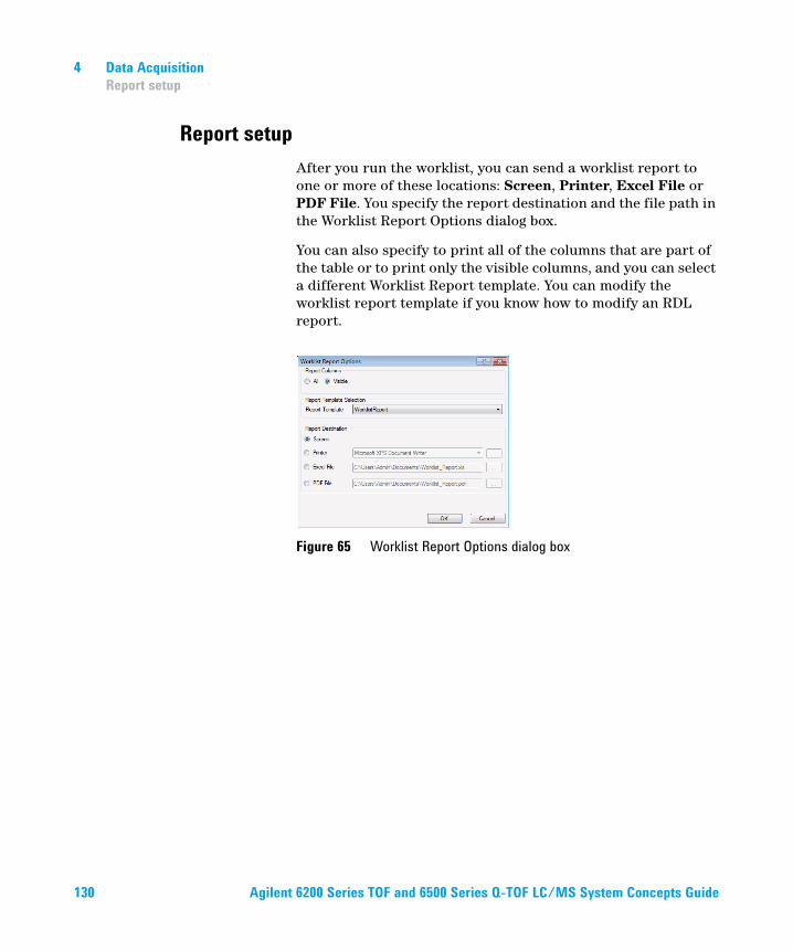
4 Data Acquisition
Report setup
Report setup
After you run the worklist, you can send a worklist report to one or more of these locations: Screen, Printer, Excel File or PDF File. You specify the report destination and the file path in the Worklist Report Options dialog box.
You can also specify to print all of the columns that are part of the table or to print only the visible columns, and you can select a different Worklist Report template. You can modify the worklist report template if you know how to modify an RDL report.
Figure 65 Worklist Report Options dialog box
130 Agilent 6200 Series TOF and 6500 Series Q-TOF LC/MS System Concepts Guide
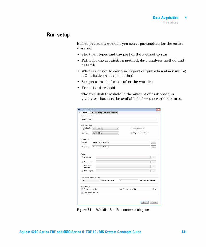
Data Acquisition 4
Run setup
Run setup
Before you run a worklist you select parameters for the entire worklist.
• Start run types and the part of the method to run
• Paths for the acquisition method, data analysis method and data file
• Whether or not to combine export output when also running a Qualitative Analysis method
• Scripts to run before or after the worklist
• Free disk threshold
The free disk threshold is the amount of disk space in gigabytes that must be available before the worklist starts.
Figure 66 Worklist Run Parameters dialog box
Agilent 6200 Series TOF and 6500 Series Q-TOF LC/MS System Concepts Guide 131
4 Data Acquisition
Estimate of worklist file size
Overlapped Data Analysis with Acquisition
You can choose to start the next data acquisition run when the data analysis is complete, or for higher throughput of samples, while data analysis of the previous sample is still running.
This option is selected in the Worklist Run Parameters dialog box, in the Execution for Acquisition-DA list box. To overlap data analysis with acquisition, select Asynchronous. To cause data acquisition to wait until data analysis is complete, select Synchronous.
Overlapped Injection
You can load a sample into the sample loop during a run that is still completing. This option allows you to save time that is required to load the sample before the run.
To select this option, mark the Overlapped Injection check box in the Worklist Run Parameters. You also have to select this option in the individual methods being used in the worklist.
Estimate of worklist file size
Depending on your estimate of the file size of the worklist, you may have to change the default value of the Free Disk Threshold.
You can run a typical worklist sample to estimate the worklist file size. Then, you observe the file size in Windows Explorer, and multiply the observed file size by the number of samples in the worklist.
The data file for profile data is compressed by a factor of 3 - 20, depending on the complexity of the mass spectra acquired. This new feature greatly reduces the data storage needed for profile data.
The Instrument Mode selected for the Accurate-Mass TOF and Accurate-Mass Q-TOF also affects the size of the data file. The Agilent TOF and Q-TOF instruments now will acquire 2 times as
132 Agilent 6200 Series TOF and 6500 Series Q-TOF LC/MS System Concepts Guide
Data Acquisition 4
Estimate of worklist file size
much data when operated in the 2 GHz mode (extended dynamic range or extended mass range) or 4 times as much data when operated in the 4 GHz mode (high resolution).
For an IM-QTOF data file, the typical file size is about 3 times larger than what the equivalent non-IM LC-MS data file would have been. A typical data file is very sparse (it has a lot of zero-abundance points which are not written to disk), but how sparse depends on the sample and lots of different conditions. As an example of the size of a very complex data file, a 1 minute method was run to acquire a raw data file of an injection of an E-coli digest with collision energy applied; the data file was around 180 MBytes in size (or around 3 MBytes/sec.) Many data files are not this large or complex.
Method parameters that control file size
LC data is usually a small fraction of TOF or Q-TOF data. The size of the acquired data file depends on these TOF or Q-TOF method parameters:
• Data file storage type—Profile, Centroid, Both or None
Profile stores raw data as abundance values for evenly spaced ion flight time. Centroid stores only the assigned peaks but not the raw data. Both stores both Profile data and Centroid data. None stores no data but does store spectrum metadata and method parameters.
If you want to analyze your data in Qualitative Analysis using either the Large Molecular Feature Extractor (LMFE) algorithm or the Deconvolute (MS): Maximum Entropy algorithm, you acquire in either Profile or Both modes. Profile data is required for both of these algorithms.
• Total run time
• Setting of time segments
• Number of experiments that are defined
Agilent 6200 Series TOF and 6500 Series Q-TOF LC/MS System Concepts Guide 133
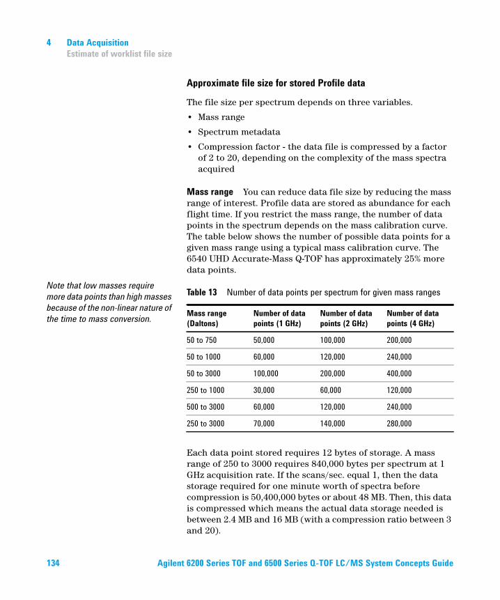
4 Data Acquisition
Estimate of worklist file size
Approximate file size for stored Profile data
The file size per spectrum depends on three variables.
• Mass range
• Spectrum metadata
• Compression factor - the data file is compressed by a factor of 2 to 20, depending on the complexity of the mass spectra acquired
Mass range You can reduce data file size by reducing the mass range of interest. Profile data are stored as abundance for each flight time. If you restrict the mass range, the number of data points in the spectrum depends on the mass calibration curve. The table below shows the number of possible data points for a given mass range using a typical mass calibration curve. The 6540 UHD Accurate-Mass Q-TOF has approximately 25% more data points.
Note that low masses require
more data points than high masses
because of the non-linear nature of
the time to mass conversion.
Each data point stored requires 12 bytes of storage. A mass range of 250 to 3000 requires 840,000 bytes per spectrum at 1 GHz acquisition rate. If the scans/sec. equal 1, then the data storage required for one minute worth of spectra before compression is 50,400,000 bytes or about 48 MB. Then, this data is compressed which means the actual data storage needed is between 2.4 MB and 16 MB (with a compression ratio between 3 and 20).
Table 13 Number of data points per spectrum for given mass ranges
Mass range
(Daltons)
Number of data
points (1 GHz)
Number of data
points (2 GHz)
Number of data
points (4 GHz)
50 to 750 50,000 100,000 200,000
50 to 1000 60,000 120,000 240,000
50 to 3000 100,000 200,000 400,000
250 to 1000 30,000 60,000 120,000
500 to 3000 60,000 120,000 240,000
250 to 3000 70,000 140,000 280,000
134 Agilent 6200 Series TOF and 6500 Series Q-TOF LC/MS System Concepts Guide
Data Acquisition 4
Estimate of worklist file size
If the run time on a run with one time segment is 5 minutes, then one run requires between 12 MB and 80 MB of disk space. A worklist with 10 samples using the same mass range requires between 120 and 800 MB of disk space. If the scan rate is set to 20 scans per second, the data file could require a large amount of disk space.
Spectrum metadata In addition to data points, information on the spectrum, such as the instrument actuals and set points, used during acquisition is stored with each spectrum. This information takes 2884 bytes per spectrum or about 8.2 MB for the worklist described above.
Storage of method parameters for each run also affects file size but to a lesser degree than the file size of the spectrum. They take up about 10,000 bytes before sample injection starts. For a 10-sample worklist, they take up less than 0.1 MB.
Approximate file size for Centroid data
Data is not stored as the abundance at evenly spaced ion flight times. Rather, peak centroids are computed first. Each data point is stored as a pair of values of mass and abundance. The data storage required is 12 bytes per detected peak in the spectrum. The number of peaks detected is dependent on the number of compound peaks in the spectrum as well as the noise in the background and the threshold set.
If the mass range is set as 250 to 3000 and the threshold is appropriate, about 3000 to 5000 peaks are detected in one spectrum. If the scans/sec. is 1, the run time 5 minutes, and ten samples are in the worklist, then the disk space needed for these samples is between 102 and 172.5 MB.
If you have a 2 GHz instrument, the disk space needed for these samples is between 204 and 345 MB. If you have a 4 GHz instrument, the disk space needed for these sample is between 408 and 690 MB.
Spectrum metadata and method parameters are also stored with centroid data and comprise a greater percent of the file size than with Profile data.
Agilent 6200 Series TOF and 6500 Series Q-TOF LC/MS System Concepts Guide 135
4 Data Acquisition
Data acquisition for samples and worklists
Data acquisition for samples and worklists
What you can monitor during a run
Tracking sample runs
The worklist shortcut menus contain an option called “Track Worklist Run” that you can turn off or on. The default position is on. With Track Worklist Run on, you can see what sample is running at any time during the worklist run.
When you start a worklist run, the first sample row turns dark blue, indicating that the sample in this row is running and data is being acquired. When the data acquisition finishes, the first sample row turns light blue to indicate that Data Analysis is running.
If you have set Execution for Acquisition-DA to Asynchronous, you will see both a dark blue and a light blue line to indicate which lines are acquiring data and analyzing data.
Monitoring the Chromatogram Plot and Spectrum Plot windows
For more information on real-time
plots, see “Real-time displays” on
page 75.
You can also monitor the TIC or EIC chromatograms, LC parameters and mass spectra for each sample during the worklist run. You can print a plot of the real-time data by clicking the File > Print > Real-time Plot Report command.
136 Agilent 6200 Series TOF and 6500 Series Q-TOF LC/MS System Concepts Guide
Data Acquisition 4
What you can do during a run
What you can do during a run
Locked Mode
You can turn Locked Mode on or off using the toolbar icons in the main toolbar. If Locked Mode is turned on, you cannot edit a worklist or method while the data is being acquired. Also, the data file is protected, so you cannot overwrite the data file if you run this method or worklist again. If Locked Mode is turned off, then you can edit the worklist during a run.
Editing current worklist during run
You can edit any sample row or batch row during a run as long as the sample is located below the first row after the running sample row. If the last selected row is executing, then all rows are locked.
When you switch to a row to edit the sample, the “Track Worklist Run” option automatically turns off. To see the sample row running after your edit, you select this tracking option again. The screen then automatically switches to that part of the worklist with the sample that is running.
Agilent 6200 Series TOF and 6500 Series Q-TOF LC/MS System Concepts Guide 137
Agilent Technologies, Inc. 2017
Printed in USA
Revision A, April 2017
*G3335-90231*G3335-90231
www.agilent.com
In This Book
The Concepts Guide presents “The Big Picture” behind the Agilent 6200 Series TOF and 6500 Series Q-TOF LC/MS system to help you to understand how to use the TOF and Q-TOF LC/MS system components.
This guide includes concepts for:
• Inner workings of the TOF and Q-TOF MS
• Instrument Preparation
• Methods with Acquisition Parameters
• Data Acquisition

Agilent Technologies, Inc. 2017
Printed in USA
Revision A, April 2017
*G3335-90231*G3335-90231
www.agilent.com