Aggregation Effect in Carbon Footprint Accounting by the Multi-

Region Input-Output Model

19th International Input-Output Conference14 June 2011

Hiroaki ShirakawaGraduate School of Environmental Studies, Nagoya

University, Japan

In collaboration with

Xin ZhouInstitute for Global Environmental Strategies, Japan

Manfred LenzenIntegrated Sustainability Analysis, University of

Sydney, Australia

Motivations

Conventional EIA and emissions accounting at firm, project or product levels.

Useful applications of IO analysis to account for both direct and indirect environmental impacts.

Limitations of IO tables for practical environmental assessment due to the aggregation of similar products, processes and sampled firms.

Aggregation error in IO analysis and its importance in environmentally extended IO analysis.

Purpose

To examine the aggregation effects in carbon footprint accounting using MRIO

To analyse the range of aggregation errors by Monte Carlo simulations; and

To find major factors influencing the size of errors.

Methodology 1

1.Carbon footprint calculation

c: carbon intensity; es: carbon footprints in region

s;: element multiplication.

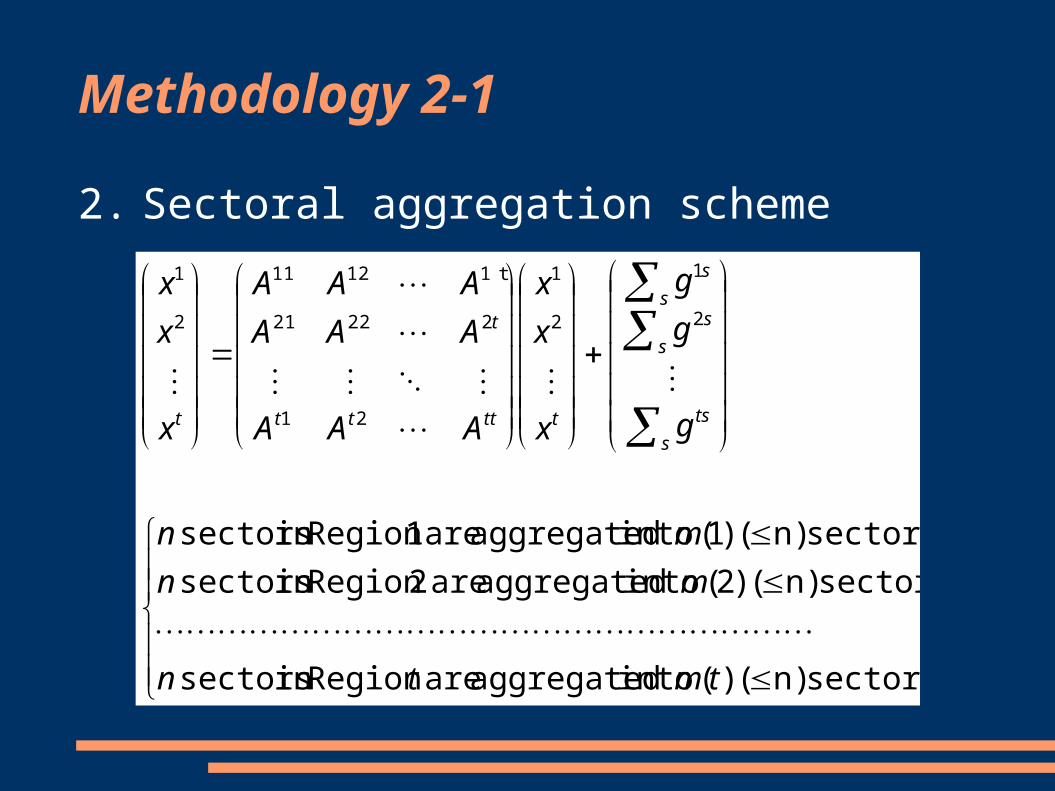
Methodology 2-1

2. Sectoral aggregation scheme

sectors. n)( )( into aggregated are Region in sectors

sectors; n)( )2( into aggregated are 2Region in sectors

sectors; n)( )1( into aggregated are 1Region in sectors

2

1

2

1

21

22221

t11211

2

1

tmtn

mn

mn

g

g

g

x

x

x

AAA

AAA

AAA

x

x

x

s

ts

s

ss

s

ttttt

t

t

Methodology 2-2

)(000

000

00)2(0

000)1(

ts

s

s

S

s(1), s(2),…, and s(t) are block summation matrices for region 1, 2, …, and t, with the size m(1)n, m(2)n, …, and m(t)n, respectively.

s’(1), s’(2),…, and s’(t) are the transposed matrices of s(1), s(2),…, and s(t), with the size nm(1), nm(2),, …, and nm(t), respectively.

Each column of the block summation matrix has one and only one number “1”. However each row can have more than one “1”, which determines which sectors to be aggregated.

)('000

000

00)2('0

000)1('

'

ts

s

s

S

Methodology 2-3

Variables Before aggregation After aggregation

Intermediate demand X Y = S X S’

Final demand g h = S g

Total output x y = S x

Carbon intensity c d = S (c x) y-1

rsijrs xXX rsijrs yYY rir ggg rir hhh rir xxx rir yyy rsijrs aAA rsijrs bBB rsijrs lLL rsijrs mMM rir ccc rir ddd sis eee sis fff

Methodology 3

3. Aggregation error and measurement

Define: aggregation error as aggregation error rate (in %) as

Method 2Method1 (Reference)

Carbon footprint calculation using the large-sized MRIO and carbon intensity

Aggregation of the large-sized MRIO table and the carbon intensity

Summation matrix S

Aggregation of regional carbon

footprints

Summation matrix S

Carbon footprint calculation using the aggregated MRIO and carbon intensity

sif

sif

)( si

si ff

si

si

si fff /)(

Data and Simulations

AIO2000 (IDE, 2006): 76 sectors and ten Asian-Pacific regions (IDN, MYS, PHL, SGP, THA, CHN, TWN, ROK, JPN, USA);

GTAP-E database on emissions intensity: 57 sectors;

Sector matching;

Determination of the summation matrix S randomly by Monte-Carlo simulations for 100,000 times

(i) Randomly determine the number of selected regions; (ii) Randomly determine which regions to be

selected; (iii) Randomly determine the number of sectors to

be aggregated for each selected region; (iv) Randomly determine which sectors to be selected

for each selected region.

Results 1-1

Aggregation error rates: Aggregated sectors (in %)

Region Minimum Average Maximum Standard Deviation

IDN -0.734 0.107 2.677 0.140MYS -12.176 0.037 11.471 0.162PHL -8.139 0.057 29.343 0.271SGP -0.438 0.066 1.885 0.162THA -2.941 0.044 165.589 0.713CHN -478.753 0.167 119.134 2.149TWN -1.384 0.072 8.798 0.119ROK -0.527 0.029 6.869 0.100JPN -7.846 0.065 4.558 0.100USA -0.355 0.092 1.574 0.088

Results 1-2

Aggregation error rates: Non-aggregated sectors (in %)

Region Minimum Average Maximum Standard Deviation

IDN -0.733 -0.023 16.585 0.162MYS -0.758 -0.040 5.779 0.118

PHL -0.669 -0.042 5.309 0.100

SGP -0.876 -0.049 3.349 0.127

THA -0.772 -0.030 6.237 0.107

CHN -0.806 -0.036 3.548 0.115

TWN -0.595 -0.031 5.072 0.094

ROK -0.681 -0.025 4.338 0.066

JPN -0.694 -0.038 2.906 0.074USA -0.826 -0.043 3.596 0.106

Results 1-3

Fig. 1 Distribution of error rates in ten economies

Fig.1 Distribution of error rates in ten economies

Indonesia Thailand Japan

Malaysia China Mainland USA

Philippines Taiwan

Error rate Error rate

Error rate

Error rate

Error rate

Error rate

Error rate

Error rate

Density (

%)

Density (

%)

Density (

%)

Density (

%)

Density (

%)

Density (

%)

Density (

%)

Density (

%)

-2 -1 0 1 2

0 5 10 15 20 25 30

Singapore Korea

Density (

%)

Density (

%)

Error rate Error rate

Results 2-2

Factors influencing the size of aggregation errors by ranking top 300 aggregation errors:

High concentrations in particular regions: CHN (140), PHL (105), IDN (22), MYS (14), ROK (13), and JPN (3) and SGP (3).

High concentrations in particular sectors: CHN (“Iron and steel”/87 times, “Chemical fertilizers and pesticides”/25 times; PHL (“Crude petroleum and natural gas”/104 times); IDN (“Iron and steel”/20 times); MYS (“Non-metallic ore and quarrying”/13 times); ROK (“Timber”/5 times); JPN (“Cement and cement products”/2 times); SGP (“Electricity and gas”/2 times, “Building construction”/2 times).

Characteristics of these sectors: relatively higher carbon intensity in their specific regions, but a less contribution to the final demand of their relevant aggregated sectors.

Conclusions

Large range of error rates (-479, 166), indicating sector aggregation has large effects on carbon footprint accounting using MRIO;

More aggregation effects on aggregated sectors than on non-aggregated sectors.

High concentration of top errors in specific regions and specific sectors, indicating their greater impacts on the size of aggregation errors. For practitioners, exclusion of these sectors in their aggregation schemes will greatly decrease the size of errors.

Relatively higher carbon intensity and relatively lower contributions to the final demand of the aggregated sectors will make a sector distinguished in terms of its effects on the size of aggregation error. For practitioners, pre-examination of this potential relationship can help find distinguished sectors during the design of aggregation scheme.

Thank you for your attention!

Contact:

Xin Zhou at zhou@iges.or.jpHiroaki Shirakawa at sirakawa@urban.env.nagoya-u.ac.jpManfred Lenzen at m.lenzen@physics.usyd.edu.au