
Aggregate Production Planning
48
Aggregate Production Planning (APP) Why aggregate planning w Details are hard to gather for longer horizons n Demand for Christmas turkeys at Tom Thumb’s vs Thanksgiving turkeys w Details carry a lot of uncertainty: aggregation reduces variability n Demand for meat during Christmas has less variability than the total variability in the demand for chicken, turkey, beef, etc. w If there is variability why bother making detailed plans, inputs will change anyway n Instead make plans that carry a lot of flexibility n Flexibility and aggregation go hand in hand
-
Upload
biswajitbanik -
Category
Documents
-
view
19 -
download
1
description
all about aggregate production planning
Transcript of Aggregate Production Planning

Aggregate Production Planning (APP)
Why aggregate planning
w Details are hard to gather for longer horizons
n Demand for Christmas turkeys at Tom Thumb’s vs Thanksgiving turkeys
w Details carry a lot of uncertainty: aggregation reduces variability
n Demand for meat during Christmas has less variability than the total variability in the demand for chicken, turkey, beef, etc.
w If there is variability why bother making detailed plans, inputs will change anyway
n Instead make plans that carry a lot of flexibility
n Flexibility and aggregation go hand in hand

Aggregate Planningw Aggregate planning: General plan
n Combined products = aggregate product
l Short and long sleeve shirts = shirt
w Single product
n Pooled capacities = aggregated capacity
l Dedicated machine and general machine = machine
w Single capacity
n Time periods = time buckets
l Consider all the demand and production of a given month together
w Quite a few time buckets [Jan/Feb… or IQ/IIQ/…]
refers to intermediate range planning covering 2 to 24 months … a “big picture” look at planning aimed at balancing capacity and demand
Aggregate Production Planning (APP)
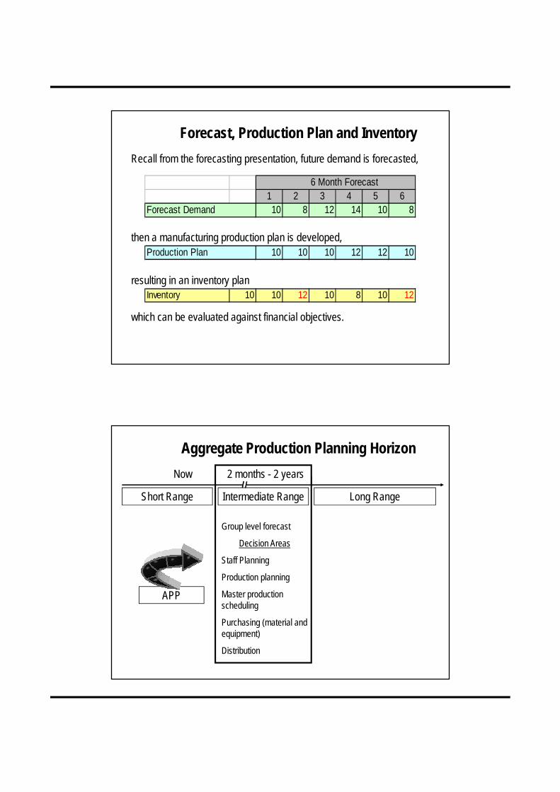
Forecast, Production Plan and Inventory
Recall from the forecasting presentation, future demand is forecasted,
6 Month Forecast1 2 3 4 5 6
Forecast Demand 10 8 12 14 10 8
Production Plan 10 10 10 12 12 10then a manufacturing production plan is developed,
Inventory 10 10 12 10 8 10 12resulting in an inventory plan
which can be evaluated against financial objectives.
Aggregate Production Planning Horizon
Group level forecast
Decision Areas
Staff Planning
Production planning
Master production scheduling
Purchasing (material and equipment)
Distribution
Short Range Intermediate Range Long Range
Now 2 months - 2 years
APP

Planning Sequence
Master scheduleEstablishes short range schedules for specific
products
Aggregate Production PlanEstablishes intermediate
range production capacity for product groups
Corporatestrategies
and policies
Economic,competitive,and political conditions
Aggregatedemand
forecasts
Business PlanEstablishes long range production and capacity strategies

Overview of Manufacturing
Planning Activities
Month J F M A M J J A S
# motors 40 25 50 30 30 50 30 40 40
Month J F M A M J J A S
# AC Motors
5 hp 15 - 30 - - 30 - - 10
25 hp 20 25 20 15 15 15 20 20 20
# DC Motors
20 hp - - - - - - 10 10 -
# WR motors
10 hp 5 - - 15 15 5 - 10 10
Master Schedule
Aggregate Plan
Note: Aggregate plan expresses the end product as “motors”
Note: Master schedule specifies precisely how many of which type (or size) of motors will be produced, and when – to plan for the material and capacity requirements
Example

Aggregate Production Planning is a planning process which establishes a company-wide game plan for allocating resources (people, equipment, etc.) and economically meeting demand. APP
. Matches market demand to company resources
. Expresses intermediate range demand, resources, and capacity in general terms – product groups or families of products rather than at the detail product level (e.g. televisions vs 21”, 27”, 32”, etc.)
. Allows planners more time to deal with short range and day-to-day issues
. Provides information to allow for flexibility … because of forecast inaccuracy intermediate plans do not have to be “locked in” too soon
Aggregate Production Planning
Supplier capabilities Storage capacity Materials availability
Materials
Current machine capacities Plans for future capacities Work-force capacities Current staffing level
Operations
New products Product design changes Machine standards
EngineeringLabor-market conditions Training capacity
Human Resources
Cost data Financial condition of firm
Accounting & Finance
APP
Customer needs Demand forecasts Competition behavior
Distribution & Marketing
Managerial Inputs to APP

The Process of APP:
. Use the company forecast to determine demand for each period
. Determine capacities (regular time, overtime, subcontracting, etc) for each period
. Identify company or departmental policies that are pertinent(employment policies, safety stock policies, etc.)
. Determine unit costs for regular time, overtime, subcontracting, holding inventories, layoffs, and other relevant costs
. Develop alternatives with cost for each
. If satisfactory plans emerge select the one that best satisfies objectives; otherwise, continue with the previous step.
Aggregate Production Planning Process
PRODUCTIONPLANNING
CAPACITY
WORK FORCE
PRODUCTION
INVENTORY
INTERNAL
EXTERNAL
EXTERNALCAPACITY
COMPETITIONRAW MATERIAL
SUPPLYDEMAND
ECONOMICCONDITIONS
Production Planning Environment
Aggregate Planning ProcessAggregate Planning Process

No
APP Process
Determine requirements for planning horizon
Identify alternatives, constraints and costs
Prepare prospective plan for planning
horizon
Is the plan acceptable?
Yes
Implement and update the plan
Move ahead to the next planning session
Aggregate Planning Objectives
The overriding objective of Aggregate Production Planning is to consider company policies and management inputs related to operations, distribution & marketing, materials, accounting & finance, engineering and human resources to
. Minimize costs & maximize profits
. Maximize customer service
. Minimize inventory investment
. Minimize changes in production rates
. Minimize changes in work-force levels
. Maximize utilization of plant and equipment

Aggregate Production Planning (APP)
Operations Managers try to determine the best way to meet forecasted demand by adjusting various capacity.
Strategies for meeting uneven supply & demand
Level capacity - maintain a level (steady rate) of production output while meeting variations in demand – [that is, use inventory to absorb fluctuations in demand]
Aggregate Planning … balancing demand/capacity
Time
Level production capacity
Demand
Uni
ts

Effect Of “Level Output Strategy”
a level output strategy – make the same amount each period
6 Month ForecastPlanning Period 1 2 3 4 5 6Forecasted Demand 10 8 12 14 10 8
Production Plan 10 10 10 10 10 10
inventory is used to “buffer” the difference in capacity and demand
Inventory Position 10 10 12 10 6 6 8
Leveling strategies try to keep output (production levels) constant and use other methods for dealing with the fluctuating demand. These strategies may be either aggressive or reactive, or a combination of both.
One popular way is to build inventory in low demand times and draw it down in high demand times.
Extreme AP Strategies- Constant Output and Constant Capacity
Inventory
DemandCapacity = Output
Cost Increased
Inventory Holding Cost/ Back-Order Cost
Costs Minimized
Hiring & Firing Cost/ Subcontracting CostOvertime- Idle Time Cost
Use When Inventory Holding Cost is LowFor High Capital Intensive Operations
Examples Water Purification Plant
Extreme AP Strategy- Variable Output and Constant Capacity
Idle TimeOvertime
Output Capacity
Demand
Cost Increase
Overtime and Idle Time CostSubcontracting Cost
Costs Minimized
Inventory Holding CostHiring/ Firing Cost
Use When Inventory is Impossible or ExpensiveFor High Skilled Labor Intensive Operations
Examples Law Firms, Accounting Service

Strategies for meeting uneven supply & demand
Chase demand - match production capacity to demand by adjusting capacity to the demand for the period
Aggregate Planning … balancing demand/capacity
Time
Uni
ts
Production chases demand
Demand
Effect Of “Chase Demand Strategy”
a chase demand strategy – production is adjusted to meet demand
6 Month ForecastPlanning Period 1 2 3 4 5 6Forecasted Demand 10 8 12 14 10 8
Production Plan 10 8 12 14 10 8
inventory remains constant
Inventory Position 10 10 10 10 10 10 10

Cost Increase
Hiring & Firing Cost/ Idle Capacity Cost
Costs Minimized
Inventory Holding Cost/ Subcontracting Cost
Overtime and Idle Time Cost
Use Inventory is Impossible or Expensive
Low Skilled Labor Operations
There is a match between Labor Availability and the Need for Labor
Examples Entertainment Center (Disney World), Farm Workers
Chase demand (Ideal Case)- change workforce levels so that production matches demand
Strategies for meeting uneven supply & demand
Demand Options … when capacity and demand are not the same
. Pricing can be adjusted to affect demand (e.g. lower rates in off season)
. Promotions (e.g. advertising, consumer marketing campaigns)
. Back Orders - shift demand to another period by taking orders in one period and promising deliver in a future period when capacity is available (may not create a satisfied customer)
. New demand - create a new need for capacity by producing a product during slack times to utilize resources (e.g. snow blower company produces leaf blowers in off season) .
Aggregate Planning … balancing demand/capacity

Strategies for meeting uneven supply & demand
Capacity Options … when capacity and demand are not the same
. Hire or lay-off workers (may create morale and employment problems
. Use overtime or under-time
. Part-time workers
. Manage capacity with inventory (e.g. let inventories build during periods of low demand or deplete during periods of high demand)
. Subcontract temporary capacity
Aggregate Planning … balancing demand/capacity
Level Strategy
Chase Strategy
Production equals
demand
Production rate is constant
Strategy Details

APP Strategies - Pure StrategiesCapacity Options — Change Capacity [Reactive Strategies]
1) changing inventory levels
2) varying work force size by hiring or layoffs
3) varying production capacity through overtime or idle time
4) subcontracting
5) using part-time workers
The above five pure strategies are called “passive strategies” because they do not try to change demand but attempt to absorb the fluctuations in it.

Reactive Strategy ExamplesReactive Strategy Examples
w Anticipation inventory is a reactive strategy. It can absorb uneven rates of demand or supply. Thus it is also a leveling strategy .
w Workforce adjustment (use of overtime, under-time or subcontracting) is reactive.
n If you are varying your workforce it is also chase. If you subcontract, it is leveling.
w Scheduling employee vacations for low demand times is a reactive strategy.
w Using backorders in high-demand times is a leveling and a reactive strategy.
¨ Demand Options — change demand [Proactive Strategies]
6) influencing demand
7) backordering during high demand periods
8) Counter seasonal product mixing
APP Strategies - Pure Strategies
The above three pure strategies are called “active strategies” through which firms try to influence the demand pattern to smooth out its changes over the planning period.

ww The purpose of aggressive strategies is to influence The purpose of aggressive strategies is to influence demand in order to smooth out (demand in order to smooth out (levellevel) production or ) production or service flow. service flow. ((All aggressive strategies are All aggressive strategies are levelingleveling.).)
ww Product Promotions Product Promotions are designed to increase sales using are designed to increase sales using creative pricing. Doing so in a low demand period is a creative pricing. Doing so in a low demand period is a leveling leveling strategy.strategy.
nn OffOff--season rates: (January retail sales) (slowseason rates: (January retail sales) (slow--season season resort rates)resort rates)
ww Complementary productsComplementary products: Services or products that have : Services or products that have similar resource requirements but different demand cycles similar resource requirements but different demand cycles allow allow leveling leveling of output.of output.
nn EG: counterEG: counter--seasonal products or services such as seasonal products or services such as seasonal clothing.seasonal clothing.
Aggressive StrategiesAggressive Strategies
Planning Strategies SummarizedPlanning Strategies SummarizedReactive Strategies
w Hiring & Layoffs (Chase)
w Overtime & Idle time (Chase)
w Subcontracting (Leveling)
w Back Orders (Leveling)
w Inventory Levels (Leveling) (Creating more inventory in slow periods and using it to meet excess demand in high demand periods.)
Aggressive Strategies
w Pricing (Leveling)
w Promotion (Leveling)
w Complementary (counter-seasonal) Products(Leveling)
Most planning strategies are not Pure (one kind). They are usually Hybrid Strategies with a combination of techniques, often using leveling and chase.

Aggregate Scheduling Options/Strategies :Advantages & Disadvantages
Option Advantage Disadvantage SomeComments
Changinginventory levels
Changes inhuman resourcesare gradual, notabruptproductionchanges
Inventoryholding costs;Shortages mayresult in lostsales
Applies mainlyto production,not service,operations
Varyingworkforce sizeby hiring orlayoffs
Avoids use ofother alternatives
Hiring, layoff,and trainingcosts
Used where sizeof labor pool islarge
Aggregate Scheduling Options/Strategies :Advantages & Disadvantages
Option Advantage Disadvantage SomeComments
Varyingproduction ratesthrough overtimeor idle time
Matches seasonalfluctuationswithouthiring/trainingcosts
Overtimepremiums, tiredworkers, may notmeet demand
Allowsflexibility withinthe aggregateplan
Subcontracting Permitsflexibility andsmoothing of thefirm's output
Loss of qualitycontrol; reducedprofits; loss offuture business
Applies mainlyin productionsettings
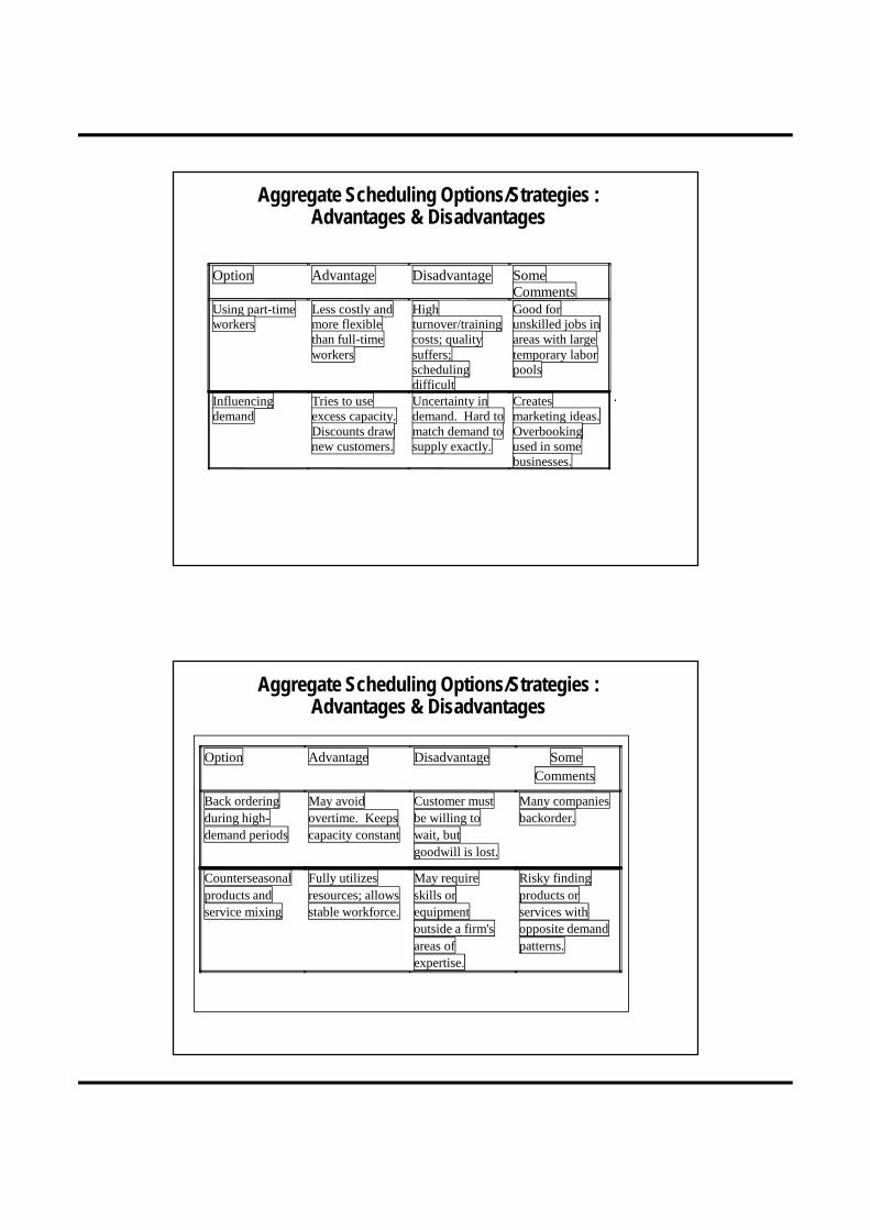
Aggregate Scheduling Options/Strategies :Advantages & Disadvantages
Option Advantage Disadvantage SomeComments
Using part-timeworkers
Less costly andmore flexiblethan full-timeworkers
Highturnover/trainingcosts; qualitysuffers;schedulingdifficult
Good forunskilled jobs inareas with largetemporary laborpools
Influencingdemand
Tries to useexcess capacity.Discounts drawnew customers.
Uncertainty indemand. Hard tomatch demand tosupply exactly.
Createsmarketing ideas.Overbookingused in somebusinesses.
Aggregate Scheduling Options/Strategies :Advantages & Disadvantages
Option Advantage Disadvantage SomeComments
Back orderingduring high-demand periods
May avoidovertime. Keepscapacity constant
Customer mustbe willing towait, butgoodwill is lost.
Many companiesbackorder.
Counterseasonalproducts andservice mixing
Fully utilizesresources; allowsstable workforce.
May requireskills orequipmentoutside a firm'sareas ofexpertise.
Risky findingproducts orservices withopposite demandpatterns.

The Reality of Planning StrategyThe Reality of Planning Strategyw Most Aggregate Planning (Production and Staffing) is
Trial and Error planning.
w Process-Focused firms are more apt to use Chasestrategies. (Chasing/reacting to demand)
n Process-focused firms are smaller and more adaptable to changing demand and more flexible in making capacity change. (Wait-and-see capacity planning)
w Product-Focused Firms are more apt to use Levelingstrategies. (Keeping output level)
n High volume, lower inventories, lower margins and higher equipment-utilization needs make it more difficult and costly to vary production rates.
No allowances are made for holidays, different number of workdays
Cost is a linear function composed of unit cost & number of units
Plans are feasible (e.g. sufficient inventory storage space is available, subcontractors are available to produce quantity and quality of products, changes in output can be made as needed)
Cost figures can be reasonably estimated and are constant for the planning horizon
Inventories are built and drawn down at a uniform rate and output occurs at a uniform rate though out
Aggregate Planning assumptions

1. Informal, trial and error methods. In practice, these techniques are more commonly used.
2. Mathematical techniques - such as linear programming, linear decision rules or simulation. Although not widely used, they serve as a basis for comparing the effectiveness of alternative techniques for aggregate planning.
General Procedure for Aggregate Planning
1. Determine demand and production requirements for each period.
2. Determine production capacity (regular time, overtime, subcontracting) for each period.
3. Determine company or departmental policies that are pertinent.
For example, maintain a safety stock of 5 percent of demand, or maintain a reasonably stable work force.
4. Determine unit costs for regular time, overtime, subcontracting, holding inventories, back orders and other relevant costs.
5. Develop alternative plans and compute the cost of each.
6. If satisfactory plans emerge, select the one that best satisfies objectives (such as cost minimization). Otherwise, return to step 5.
Techniques for Aggregate Production Planning
Simple tables or worksheets can be developed to evaluate demand, aggregate group level production plans and inventory. We will look at some examples to illustrate the concept of aggregate planning. The assumptions for these examples simplify the computations but can be easily modified to “real situations”.
Aggregate Planning – Informal Techniques

Aggregate Planning – Informal Techniques
Aggregate Planning - formula’s
Number of workers in period = Number of workers at end of the previous period + Number of new workers at the start of a period - Number of laid-off workers at the start of a period
Inventory at the end of a period = Inventory at the end of the previous period + Production in the current period - Amount used to satisfy demand in the
current period
Average Inventory for a period = (Beginning Inventory + Ending Inventory) / 2
Cost for a period = Output Cost + Hire/Lay-off Cost + Inventory Cost + Backorder Cost where Output Cost = Regular Time Cost + Overtime Cost + Subcontractor Cost
How To Calculate Costs …
Regular Costs. Output cost = Regular cost per unit * Quantity of regular output. Overtime cost = Overtime cost per unit * Overtime quantity. Subcontract cost = Subcontract cost per unit * Subcontract quantity
Hire-Layoff Costs. Hire cost = Cost per hire * Number hired. Lay-off cost = Cost per lay-off * Number laid off
Inventory Costs. Carrying cost per unit * Average inventory
Back Order Costs. Back order cost per unit * Backorder quantity

Aggregate Production Planning Illustration
Given the following information:
6 month production planning period
10 labour-hours per unit required
Labour cost = $10/hour regular= $15/hour overtime
Total unit cost = $200 / unit= $228/unit subcontract
Current workforce = 20 employees
Hiring cost = $500 / employee
Layoff cost = $800 / employee
Safety stock = 20% of monthly forecast
Beginning inventory = 50 units
Inventory carrying cost = $10/unit/month
Stockout cost = $50/unit/month
Additional information available:Sales Work Work Hours
Month Forecast Days at 8 Hrs. / DayJan. 300 22 176Feb. 500 19 152Mar. 400 21 168Apr. 100 21 168May. 200 22 176June 300 20 160
First Step: Calculate Production Requirement
Sales Safety ProductionMonth Forecast Stock RequiredJan. 300 60 300+60-50 = 310Feb. 500 100 500+100-60 = 540 Mar. 400 80 400+80-100 = 380Apr. 100 20 100+20-80 = 40May. 200 40 200+40-20 = 220 June 300 60 300+60-40 = 320
Safety Stock of the period t will be an Beginni9ng Inventory of the period (t+1)
ProductionRequired
31054038040220320
HoursRequired
310054003800400
22003200
Hrs. Avail.per Worker
176152168168176160
WorkersRequired
18362331320
WorkersHired
18
107
WorkersFired
2
1320
Hire/FireCosts
$16009000
10400 16000 50003500
Total Cost = $45,500
ProductionRequired
31054038040220320
HoursRequired
31005400380040022003200
Total Hrs.Available
352030403360336035203200
OvertimeHours
2360440
UndertimeHours420
29601320
OT/ UTCosts$420011800
2200148006600
0
Plan # 2 - Exact Production; Vary Production Rate
Total Cost = $61,000
MonthJan.Feb.Mar.Apr.MayJune
MonthJan.Feb.Mar.Apr.MayJune
Plan # 1 - Exact Production; Vary Work Force
Aggregate Production Planning Illustration – Contd.

Cum. Prod.Required
310850
1230127014901810
TotalProduction
352304336336352320
CumulativeProduction
352656992
132816802000
InventoryLevel
42
58190190
StockoutLevel
194238
Inv. / SOCosts$4209700
11900 580
19001900
Total Cost = $26,400
HoursAvailable
352030403360336035203200
Total Cost = $7,160 + $ 21,000 = $28,160
Cum. Prod.Required
310850
1230127014901810
HoursAvailable3520(20)4560(30)5040(30)1680(10)1760(10)1600(10)
TotalProduction
352456504168176160
Cumulative Production
352808
1312 1480 1656 1816
Inv. / (SO) Level42
(42)82210166
6
Inv. / SOCosts$4202100820
2100 1660
60
Hire/FireCosts
5000
16000
$7,160 $21,000
MonthJan.Feb.Mar.Apr.MayJune
MonthJan.Feb.Mar.Apr.MayJune
Plan # 3 - Exact Production; Vary Inventory Level With 20 Employees
Aggregate Production Planning Illustration – Contd.
Plan # 4 - Exact Production; Vary Workforce Level; Vary Inventory Level
PlanCosts
45,50061,00026,40028,160
Plan1234
ProductionCosts
362,000362,000400,000363,200
TotalCosts
407,500446,500426,400391,360
UnitsProduced
1810181020001816
Costper Unit$225.14$233.70$213.20$215.51
Final Cost Analysis:
Decision: Go with Plan # 3 on the basis of lowest cost per unit.
Aggregate Production Planning Illustration - Contd.

Example 2: Planners for a company that makes several models of tractors are about to prepare an aggregate plan that will cover 6 periods. The have assembled the following cost information ($):
Output CostsRegular time 2 per tractorOvertime 3 per tractorSubcontract 6 per tractor
Inventory Costs1 per tractor on average inventory Back Order Costs 5 per tractor per period
The forecasted demand by period is:
Aggregate Planning – Example 2
Planning Period 1 2 3 4 5 6 TotalForecasted Demand 200 200 300 400 500 200 1800
They now want to evaluate a plan that calls for a steady rate of regular-time output.
They intend to start with 0 inventory on hand in the first period.
Prepare an aggregate plan and determine its cost for a level output rate of 300 units per period with 15 workers.
Aggregate Planning – Example 2

Aggregate Planning
Total cost of plan is $4,700
Inventory
Backorder
Costs
Production Schedule
Cumulative Forecast & Production
Cost Components Notice the backorder
cost in period 5
Example 2: After reviewing the plan the planners need to develop an alternative based on the news that one of the regular time workers has decided to retire.
Rather than replace that person they would rather stay with a smaller work force and use overtime to make up for the lost output.
The maximum overtime output is 40 units.
Aggregate Planning – Example 2
First the regular time output of 300 units per 15 people must be adjusted for 14 people. Therefore 300/15*14 = 280 = adjusted regular time output for 14 people.

We are 120 tractors short.
Where do we manufacture them?
Aggregate Planning
Why did we put manufacture them here?
Does manufacturing them in other periods produce a lower cost?
Total cost of plan is $4,640
Aggregate Planning
Notice the backorder cost in period 5
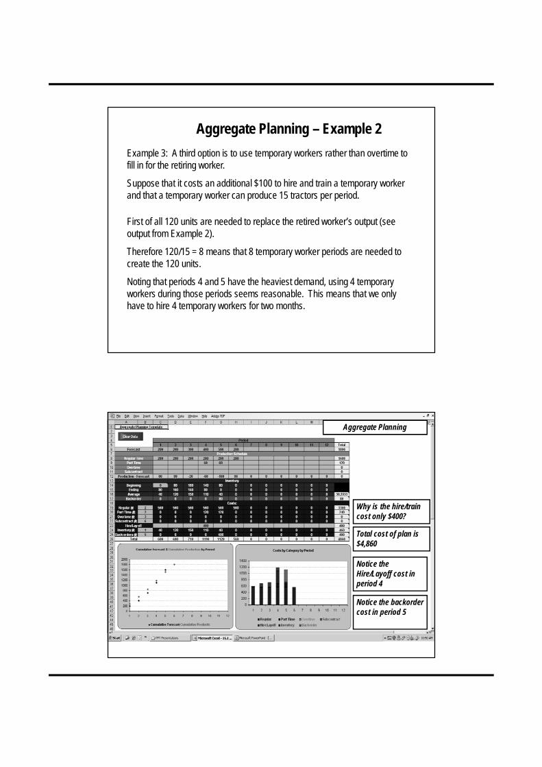
Example 3: A third option is to use temporary workers rather than overtime to fill in for the retiring worker.
Suppose that it costs an additional $100 to hire and train a temporary worker and that a temporary worker can produce 15 tractors per period.
Aggregate Planning – Example 2
First of all 120 units are needed to replace the retired worker’s output (see output from Example 2).
Therefore 120/15 = 8 means that 8 temporary worker periods are needed to create the 120 units.
Noting that periods 4 and 5 have the heaviest demand, using 4 temporary workers during those periods seems reasonable. This means that we only have to hire 4 temporary workers for two months.
Why is the hire/train cost only $400?
Total cost of plan is $4,860
Aggregate Planning
Notice the backorder cost in period 5
Notice the Hire/Layoff cost in period 4

Pure Strategies
Hiring costHiring cost = $100 per worker= $100 per workerFiring costFiring cost = $500 per worker= $500 per worker
Regular production cost per pound = $2.00Regular production cost per pound = $2.00Inventory carrying costInventory carrying cost = $0.50 pound per quarter= $0.50 pound per quarter
Production per employeeProduction per employee = 1,000 pounds per quarter= 1,000 pounds per quarterBeginning work forceBeginning work force = 100 workers= 100 workers
QUARTERQUARTER SALES FORECAST (LB)SALES FORECAST (LB)
SpringSpring 80,00080,000SummerSummer 50,00050,000FallFall 120,000120,000WinterWinter 150,000150,000
Example:Example:
Level Production Strategy
Level production
= 100,000 pounds(80,000 + 50,000 + 120,000 + 150,000)
4
SpringSpring 80,00080,000 100,000100,000 20,00020,000SummerSummer 50,00050,000 100,000100,000 70,00070,000FallFall 120,000120,000 100,000100,000 50,00050,000WinterWinter 150,000150,000 100,000100,000 00
400,000400,000 140,000140,000
Cost of Level Production Strategy:
(400,000 X $2.00) + (140,00 X $.50) = $870,000
SALESSALES PRODUCTIONPRODUCTIONQUARTERQUARTER FORECASTFORECAST PLANPLAN INVENTORYINVENTORY

Chase Demand Strategy
SpringSpring 80,00080,000 80,00080,000 8080 00 2020SummerSummer 50,00050,000 50,00050,000 5050 00 3030FallFall 120,000120,000 120,000120,000 120120 7070 00WinterWinter 150,000150,000 150,000150,000 150150 3030 00
100100 5050
SALESSALES PRODUCTIONPRODUCTION WORKERSWORKERS WORKERSWORKERS WORKERSWORKERSQUARTERQUARTER FORECASTFORECAST PLANPLAN NEEDEDNEEDED HIREDHIRED FIREDFIRED
Cost of Chase Demand Strategy
(400,000 X $2.00) + (100 x $100) + (50 x $500) = $835,000
Previous Spring Summer Fall WinterBeginning Inventory 0 10,000 40,000 30,000Demand Forecast 80,000 50,000 120,000 150,000Production Plan 90,000 80,000 110,000 120,000Ending Inventory 0 10,000 40,000 30,000 0Work-force Size 100 90 80 110 120
Total Demand Forecast= 400,000Total Production Plan= 400,000
Inventory Cost (.50/lb) $5,000 $20,000 $15,000 $0Work-force Cost $5,000 $5,000 $3,000 $1,000Total Cost $54,000
Quarter
Mixed Strategy
Initial Inv (t) = End Inv (t-1)

Mixed Strategy• Combination of Level Production and Chase
Demand strategies
• Examples of management policies
– no more than x% of the workforce can be laid off in one quarter
– inventory levels cannot exceed x dollars
• Many industries may simply shut down manufacturing during the low demand season and schedule employee vacations during that time
APP Using Mixed Strategies - Exercise
Production per employee= 100 cases per monthWage rate = $10 per case for regular production
= $15 per case for overtime= $25 for subcontracting
Hiring cost = $1000 per workerFiring cost = $500 per worker
Inventory carrying cost = $1.00 case per monthBeginning work force = 10 workers
January 1000 July 500February 400 August 500March 400 September 1000April 400 October 1500May 400 November 2500June 400 December 3000
MONTH DEMAND (CASES) MONTH DEMAND (CASES)

Mathematical Model
u Data:
– Starting inventory in January: 1,000 units
– Selling price to the retailer: Rs.40/unit
– Workforce at the beginning of January: 80
– # of working days per month: 20
– Regular work per day per employee: 8 hours
– Maximum overtime allowed per employee per month: 10 hours
– Ending inventory required (at end of June): Minimum 500 units
– Demand forecast:
Month January February March April May June
Demand 1,600 3,000 3,200 3,800 2,200 2,200

Numerical Example
Item Cost Materials Rs.10/unit Inventory holding cost Rs.2/unit/month Marginal cost of a stockout Rs.5/unit/month Hiring and training costs Rs.300/worker Layoff cost Rs.500/worker Labor hours required 4/unit Regular time cost Rs.4/hour Over time cost Rs.6/hour Cost of subcontracting Rs.30/unit
(cont…)
u Cost Data:
Numerical Example (Define Decision Variables)
• The decision variables are as follows:
– Wt = Workforce size for month t
– Ht = Number of employees hired at the beginning of month t
– Lt = Number of employees laid off at the beginning of month t
– Pt = Production in month t
– It = Inventory at the end of month t
– St = Number of units stocked out at the end of month t
– Ct = Number of units subcontracted for month t
– Ot = Number of overtime hours worked in month t
(combined for all employees)
Note: For all the above variables, t = 1, 2, …, 6 giving a total of
48 decision variables.
Numerical Example (Components of Objective Function)
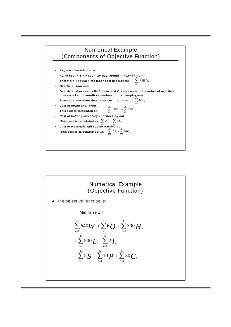
• Regular time labor cost
Rs. 4/hour * 8 hr/day * 20 day/month = Rs.640/month
Therefore, regular time labor cost per month:
• Overtime labor cost
Overtime labor cost is Rs.6/hour and Ot represents the number of overtime hours worked in month t (combined for all employees)
Therefore, overtime time labor cost per month:
• Cost of hiring and layoff
This cost is calculated as:
• Cost of holding inventory and stocking out
This cost is calculated as:
• Cost of materials and subcontracting out
This cost is calculated as: 15
å=
6
1tW640
t
å=
6
1tO6
t
åå==
+6
1t
6
1t L500H300
tt
åå==
+6
1t
6
1t S5I2
tt
åå==
+6
1t
6
1t C30P10
tt
Numerical Example(Objective Function)
ååå
åå
ååå
===
==
===
+++
++
++
6
1
6
1
6
1
6
1
6
1
6
1
6
1
6
1
30105
2500
3006640
tt
tt
tt
tt
tt
tt
tt
tt
CPS
IL
HOW
u The objective function is:
Minimize Z =

Numerical Example (Define Constraints Linking Variables)
• Workforce size, hiring and layoff constraints:
or
where t = 1, 2, …, 6 and W0 = 80
• Capacity constraints:
or
where t = 1, 2, …, 6
0LHWW tt1tt =++- -
tt1tt LHWW -+= -
ttt O)4/1(W40P +£
0PO)4/1(W40 ttt ³-+
• Inventory balance constraints:
or
where t = 1, 2, …, 6 and I0 = 1,000, I6 >= 500, and S0 = 0,
• Overtime limit constraints:
or
where t = 1, 2, …, 6
tt1tttt1-t SISDCPI -++=++ -
0SISDCPI tt1tttt1-t =+---++ -
tt W10O £
0W10O tt £-
Numerical Example (Define Constraints Linking Variables) (cont…)

Average Inventory and Average Flow Time
• Average inventory for a period t:
• Average inventory over the planning horizon:
i.e.
• Average flow time: (Average inventory)/(Throughput)
)I(I21
t1t +-
å=
- +T
tT 1t1t )I(I
211
úû
ùêë
é++ å
-
=-
1
1tt1t I)I(I
211 T
tT
å
å
=
-
=- ú
û
ùêë
é++
T
t
T
t
T
T
1t
1
1tt1t
D1
I)I(I211
Various Scenarios
• Some of the possible scenarios are:
– Increase in holding cost (from Rs.2 to Rs.6)
– Overtime cost drops to Rs.5 per hour
– Increased demand fluctuation
• Your plan will change with the change in scenarios
Month January February March April May June
Demand 1,000 3,000 3,800 4,800 2,000 1,400

Transportation Tableau forAggregate Planning
• Suppose we have the following information
– Beginning Inventory: I0
– Regular time production cost per unit: r
– Overtime production cost per unit: v
– Subcontract production cost per unit: s
– Holding cost per unit per period: h
– Backorder cost per unit per period: b
– Shortage (unsatisfied order) cost per unit per period: c
– Undertime cost per unit: u
– Desired inventory level at the end of period 3: Ie
– Total unused capacities: U
– Total unsatisfied orders: C
Periods
1 2 3
Demand D1 D2 D3
Regular Capacity R1 R2 R3
Overtime Capacity O1 O2 O3
Subcontract Capacity S1 S2 S3
LINEAR PROGRAMMING(no backorders, supply > demand)
Beg. Inventory
Demand for
Period 1 Period 2 Period 3
TotalCapacity(supply)
UnusedCapacitySupply from
v v + h v + 2h
0 h 2h
s s + h s + 2h
v v + h
r r + h r + 2h
v
r r + h
s s + h
s
r
Regular
Overtime
Subcontract
Regular
Overtime
Subcontract
Regular
Overtime
Subcontract
I0
R1
O1
S1
R2
O2
S2
R3
O3
S3
u
u
u
u
u
u
u
u
u
u
Demand D1 D2 D3 + le U Grand Total
1
2
3

LINEAR PROGRAMMING(backorders, supply > demand)
Beg. Inventory
Demand for
Period 1 Period 2 Period 3
TotalCapacity(supply)
UnusedCapacitySupply from
v v + h v + 2h
0 h 2h
s s + h s + 2h
v + b v v + h
r r + h r + 2h
v + 2b v + b v
r + b r r + h
s + b s s + h
s + 2b s + b s
r + 2b r + b r
Regular
Overtime
Subcontract
Regular
Overtime
Subcontract
Regular
Overtime
Subcontract
I0
R1
O1
S1
R2
O2
S2
R3
O3
S3
u
u
u
u
u
u
u
u
u
u
Demand D1 D2 D3 + le U Grand Total
1
2
3
Beg. Inventory
Demand for
Period 1 Period 2 Period 3
TotalCapacity(supply)
Supply from
Regular
Overtime
Subcontract
Regular
Overtime
Subcontract
Regular
Overtime
Subcontract
I0
R1
O1
S1
R2
O2
S2
R3
O3
S3
C
Demand D1 D2 D3 + le Grand Total
v v + h
0 h 2h
s s + h
r r + h
v v + h v + 2h
s s + h s + 2h
r r + h r + 2h
r
v
s
LINEAR PROGRAMMING(no backorders, demand > supply)
Unsatisfied Demand c c c
1
2
3

Demand1 2 3 4 5 6 7 8 9 Total190 230 260 280 210 170 160 260 180 1940
There are 20 full time employees, each can produce 10 units per period at the cost of $6 per unit. Therefore the supply of full time workers is as follows1 2 3 4 5 6 7 8 9 Total200 200 200 200 200 200 200 200 200 1800
Overtime cost is $13 per unit. Inventory carrying cost $5 per unit per periodBacklog cost $10 per unit per period
Maximum over time production is 20 units per period
Formulated the problem as a Linear Programming model.
Exercise
APP by the Transportation Method
1 900 1000 100 5002 1500 1200 150 5003 1600 1300 200 5004 3000 1300 200 500
Regular production cost per unit $20Overtime production cost per unit $25Subcontracting cost per unit $28Inventory holding cost per unit per period $3Beginning inventory 300 units
EXPECTED REGULAR OVERTIME SUBCONTRACTQUARTER DEMAND CAPACITY CAPACITY CAPACITY
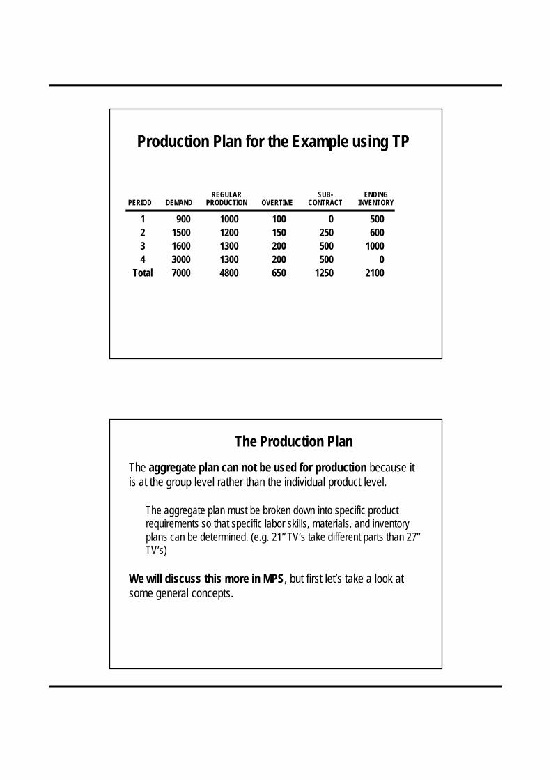
Production Plan for the Example using TP
1 900 1000 100 0 5002 1500 1200 150 250 6003 1600 1300 200 500 10004 3000 1300 200 500 0
Total 7000 4800 650 1250 2100
REGULAR SUB- ENDINGPERIOD DEMAND PRODUCTION OVERTIME CONTRACT INVENTORY
The aggregate plan can not be used for production because it is at the group level rather than the individual product level.
The aggregate plan must be broken down into specific product requirements so that specific labor skills, materials, and inventory plans can be determined. (e.g. 21” TV’s take different parts than 27” TV’s)
We will discuss this more in MPS, but first let’s take a look at some general concepts.
The Production Plan

Because different products require different materials, skills, etc. we must manufacture at the item level rather than the group level. The master schedule (item level) is similar to the aggregate plan (group level).
. Master Schedule - is a detailed plan usually done for weekly periods(sometimes daily) showing the quantity and timing of specific items (e.g. 21” TV’s) for a scheduled horizon and can be used by other functional areas of the organization.
. Rough-Cut Capacity Planning - is an approximate balancing of the detailed master production schedule with capacity to test the feasibility of the master production schedule. It resembles the aggregate planning
process; but, at a detailed product level.
The Production Plan
Masterscheduling
Beginning Inventory
Forecast
Customer Orders
Inputs
3 inputs and 3 outputs
Master Scheduling Process
Outputs
Projected Inventory
Master Production Schedule
Available To Promise
(uncommitted inventory)

Projected demand is calculated based on the customer orders and forecast.
Projected Demand = max (forecast, orders)
Inputs To Master Scheduling
Planning Period 1 2 3 4 5 6 7 8Forecast 30 30 30 30 40 40 40 40
Customer Orders 33 20 10 4 2Projected Demand 33 30 30 30 40 40 40 40
Projected On Hand Inventory 64
How can customer orders be more than forecast?
Therefore, the Projected Inventory Position (previous inventory position - projected demand) without any production can be calculated and is shown below:
Outputs Of Master Scheduling
Planning Period 1 2 3 4 5 6 7 8Forecast 30 30 30 30 40 40 40 40
Customer Orders 33 20 10 4 2Projected Demand 33 30 30 30 40 40 40 40
Projected On Hand Inventory 64 31 1 -29 -59 -99 -139 -179 -219

If the lot size for this item is 70 units, we can now build the Master ProductionSchedule. We add our first lot in week/day 3 because this is the first negative inventory position. We then update our Projected Inventory Position.
Outputs Of Master Scheduling
Planning Period 1 2 3 4 5 6 7 8Forecast 30 30 30 30 40 40 40 40
Customer Orders 33 20 10 4 2Projected Demand 33 30 30 30 40 40 40 40
Projected On Hand Inventory 64 31 1 41 11 -29 -69 -109 -149Master Production Schedule (MPS) 70
Outputs Of Master Scheduling
We add our next lot in week/day 5 because this is the next negative inventory position. We then update our Projected Inventory Position.
Planning Period 1 2 3 4 5 6 7 8Forecast 30 30 30 30 40 40 40 40
Customer Orders 33 20 10 4 2Projected Demand 33 30 30 30 40 40 40 40
Projected On Hand Inventory 64 31 1 41 11 41 1 -39 -79Master Production Schedule (MPS) 70 70

We add our next lot in week/day 7 because this is the next negative inventory position. We then update our Projected Inventory Position.
Outputs Of Master Scheduling
Planning Period 1 2 3 4 5 6 7 8Forecast 30 30 30 30 40 40 40 40
Customer Orders 33 20 10 4 2Projected Demand 33 30 30 30 40 40 40 40
Projected On Hand Inventory 64 31 1 41 11 41 1 31 -9Master Production Schedule (MPS) 70 70 70
We add our next lot in week/day 9 because this is the next negative inventory position. We then update our Projected Inventory Position, and have completed the second output of the master scheduling process, the Master Production Schedule.
Outputs Of Master Scheduling
Planning Period 1 2 3 4 5 6 7 8Forecast 30 30 30 30 40 40 40 40
Customer Orders 33 20 10 4 2Projected Demand 33 30 30 30 40 40 40 40
Projected On Hand Inventory 64 31 1 41 11 41 1 31 61Master Production Schedule (MPS) 70 70 70 70
Outputs Of Master Scheduling
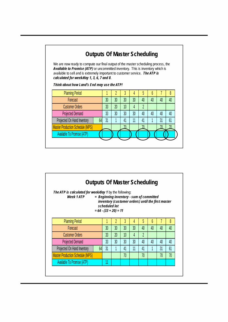
We are now ready to compute our final output of the master scheduling process, the Available to Promise (ATP) or uncommitted inventory. This is inventory which is available to sell and is extremely important to customer service. The ATP is calculated for week/day 1, 3, 6, 7 and 8.
Think about how Land’s End may use the ATP!
Planning Period 1 2 3 4 5 6 7 8Forecast 30 30 30 30 40 40 40 40
Customer Orders 33 20 10 4 2Projected Demand 33 30 30 30 40 40 40 40
Projected On Hand Inventory 64 31 1 41 11 41 1 31 61Master Production Schedule (MPS) 70 70 70 70
Available To Promise (ATP)
Outputs Of Master Scheduling
The ATP is calculated for week/day 1 by the following:Week 1 ATP = Beginning inventory - sum of committed
inventory (customer orders) until the first master scheduled lot
= 64 - (33 + 20) = 11
Planning Period 1 2 3 4 5 6 7 8Forecast 30 30 30 30 40 40 40 40
Customer Orders 33 20 10 4 2Projected Demand 33 30 30 30 40 40 40 40
Projected On Hand Inventory 64 31 1 41 11 41 1 31 61Master Production Schedule (MPS) 70 70 70 70
Available To Promise (ATP) 11

The ATP is calculated for week/day 3 by the following:Week 3 ATP = MPS for week/day 3 - sum of committed
inventory (customer orders)until the next master scheduled lot
= 70 - (10 + 4) = 56
Planning Period 1 2 3 4 5 6 7 8Forecast 30 30 30 30 40 40 40 40
Customer Orders 33 20 10 4 2Projected Demand 33 30 30 30 40 40 40 40
Projected On Hand Inventory 64 31 1 41 11 41 1 31 61Master Production Schedule (MPS) 70 70 70 70
Available To Promise (ATP) 11 56
Outputs Of Master Scheduling
Outputs Of Master Scheduling
The ATP is calculated for week/day 5 by the following:Week 5 ATP = MPS for week/day 5 - sum of committed
inventory (customer orders)until the next master scheduled lot
= 70 - 2 = 68
Planning Period 1 2 3 4 5 6 7 8Forecast 30 30 30 30 40 40 40 40
Customer Orders 33 20 10 4 2Projected Demand 33 30 30 30 40 40 40 40
Projected On Hand Inventory 64 31 1 41 11 41 1 31 61Master Production Schedule (MPS) 70 70 70 70
Available To Promise (ATP) 11 56 68

Outputs Of Master Scheduling
The ATP is calculated for week/day 7 by the following:Week 7 ATP = MPS for week/day 7 - sum of committed
inventory (customer orders)until the next master scheduled lot
= 70 - 0 = 70
Planning Period 1 2 3 4 5 6 7 8Forecast 30 30 30 30 40 40 40 40
Customer Orders 33 20 10 4 2Projected Demand 33 30 30 30 40 40 40 40
Projected On Hand Inventory 64 31 1 41 11 41 1 31 61Master Production Schedule (MPS) 70 70 70 70
Available To Promise (ATP) 11 56 68 70
Outputs Of Master Scheduling
The ATP is calculated for week/day 8 by the following:Week 8 ATP = MPS for week/day 8 - sum of committed
inventory (customer orders)until the next master scheduled lot
= 70 - 0 = 70
Planning Period 1 2 3 4 5 6 7 8Forecast 30 30 30 30 40 40 40 40
Customer Orders 33 20 10 4 2Projected Demand 33 30 30 30 40 40 40 40
Projected On Hand Inventory 64 31 1 41 11 41 1 31 61Master Production Schedule (MPS) 70 70 70 70
Available To Promise (ATP) 11 56 68 70 70

Master Scheduling
You can see by these calculations that changes to a Master Schedule can be disruptive, particularly those in the first few weeks/days of a schedule.
It is difficult to rearrange schedules, materials plans, and labor plans on a short notice.
For these reasons, many schedules have varying degrees of changes that are allowed. Time fences are created to indicate the level of change if any that will be considered .
Stabilizing The Master Schedule
Planning Period1 2 3 4 5 6 7 8 9 10 11 12
Frozen FullFirm Open

Items
Product lines or families
Individual products
Components
Manufacturing operations
Resource level
Plants
Individual machines
Critical work centers
Production Planning Capacity Planning
Resource Requirements Plan
Rough-Cut Capacity Plan
Capacity Requirements Plan
Input/Output Control
Aggregate Production Plan
Master Production Schedule
Material Requirements Plan
Shop Floor Schedule
All work centers
Hierarchical Planning Process


![[PPT]Production and Operations Management: …sureten/(aggregate planning)5.ppt · Web viewDisaggregating the Aggregate Plan Aggregate Planning Aggregate planning Intermediate-range](https://static.fdocuments.in/doc/165x107/5aec86827f8b9ab24d902697/pptproduction-and-operations-management-suretenaggregate-planning5pptweb.jpg)