Aggregate Planning and S&OP€¦ · Sales and Operations Planning 533 The Nature of Aggregate...
34
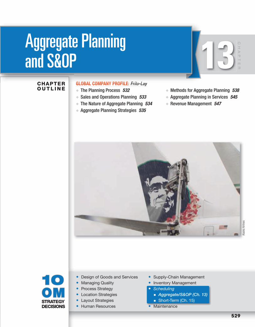
529 529 CHAPTER OUTLINE ◆ The Planning Process 532 ◆ Sales and Operations Planning 533 ◆ The Nature of Aggregate Planning 534 ◆ Aggregate Planning Strategies 535 ◆ Methods for Aggregate Planning 538 ◆ Aggregate Planning in Services 545 ◆ Revenue Management 547 GLOBAL COMPANY PROFILE: Frito-Lay CHAPTER 10 10 OM OM STRATEGY DECISIONS • • Design of Goods and Services • • Managing Quality • • Process Strategy • • Location Strategies • • Layout Strategies • • Human Resources • • Supply-Chain Management • • Inventory Management • • Scheduling · · Aggregate/S&OP (Ch. 13) · · Short-Term (Ch. 15) • • Maintenance CHAPTER GLOBAL COMPANY PROFILE Frito Lay Aggregate Planning and S&OP 13 Alaska Airlines
Transcript of Aggregate Planning and S&OP€¦ · Sales and Operations Planning 533 The Nature of Aggregate...
529529
CHAPTER O U T L I N E
The Planning Process 532
Sales and Operations Planning 533
The Nature of Aggregate Planning 534
Aggregate Planning Strategies 535
Methods for Aggregate Planning 538
Aggregate Planning in Services 545
Revenue Management 547
GLOBAL COMPANY PROFILE Frito-Lay
CH
AP
TE
R
1010OMOM STRATEGY DECISIONS
bull bull Design of Goods and Services
bull bull Managing Quality
bull bull Process Strategy
bull bull Location Strategies
bull bull Layout Strategies
bull bull Human Resources
bull bull Supply-Chain Management
bull bull Inventory Management
bullbull Scheduling
AggregateSampOP ( Ch 13 ) Short-Term ( Ch 15 )
bull bull Maintenance
CHAPTER GLOBAL COMPANY PROFILE Frito Lay
Aggregate Planning and SampOP 13
Ala
ska
Airl
ines
M17_HEIZ0422_12_SE_C13indd 529M17_HEIZ0422_12_SE_C13indd 529 051115 518 PM051115 518 PM
Like other organizations throughout the world Frito-Lay relies on effective aggregate planning
to match fluctuating multi-billion-dollar demand to capacity in its 36 North American plants
Planning for the intermediate term (3 to 18 months) is the heart of aggregate planning
Effective aggregate planning combined with tight scheduling effective maintenance and efficient
employee and facility scheduling are the keys to high plant utilization High utilization is a critical
factor in facilities such as Frito-Lay where capital investment is substantial
Frito-Lay has more than three dozen brands of snacks and chips 15 of which sell more than
$100 million annually and 7 of which sell over $1 billion Its brands include such well-known
names as Fritos Layrsquos Doritos Sun Chips Cheetos Tostitos Flat Earth and Ruffles Unique
processes using specially designed equipment are required to produce each of these products
Because these specialized processes generate high fixed cost they must operate at very high
volume But such product-focused facilities benefit by having low variable costs High utiliza-
tion and performance above the break-even point require a good match between demand and
capacity Idle equipment is disastrous
At Frito-Layrsquos headquarters near Dallas planners create a total demand profile They use
historical product sales forecasts of new products product innovations product promotions
Aggregate Planning Provides a Competitive Advantage at Frito-Lay
GLOBAL COMPANY PROFILE Frito-Lay
C H A P T E R 1 3
530
The aggregate plan adjusts for farm location
yield and quantities for timely delivery of
Frito-Layrsquos unique varieties of potatoes
During harvest times potatoes go directly
to the plant During non-harvest months
potatoes are stored in climate-controlled
environments to maintain quality texture
and taste
Frito
-Lay
Nor
th A
mer
ica
M17_HEIZ0422_12_SE_C13indd 530M17_HEIZ0422_12_SE_C13indd 530 051115 518 PM051115 518 PM
531
and dynamic local demand data from account
managers to forecast demand Planners then
match the total demand profile to existing
capacity capacity expansion plans and cost
This becomes the aggregate plan The aggre-
gate plan is communicated to each of the firmrsquos
17 regions and to the 36 plants Every quarter
headquarters and each plant modify the
respective plans to incorporate changing mar-
ket conditions and plant performance Each plant uses its quarterly plan to develop
a 4-week plan which in turn assigns specific
products to specific product lines for produc-
tion runs Finally each week raw materials and
labor are assigned to each process Effective
aggregate planning is a major factor in high
utilization and low cost As the companyrsquos 60
market share indicates excellent aggregate
planning yields a competitive advantage at
Frito-Lay
As potatoes arrive at the plant they are promptly washed and peeled to ensure freshness and taste
Frito
-Lay
Nor
th A
mer
ica
Frito
-Lay
Nor
th A
mer
ica
After peeling potatoes are cut into thin
slices rinsed of excess starch and
cooked in sunflower andor corn oil
Frito
-Lay
Nor
th A
mer
ica
After cooking is complete inspection
bagging weighing and packing
operations prepare Layrsquos potato chips
for shipment to customersmdashall in a
matter of hours Frito
-Lay
Nor
th A
mer
ica
M17_HEIZ0422_12_SE_C13indd 531M17_HEIZ0422_12_SE_C13indd 531 051115 518 PM051115 518 PM
532
The Planning Process In Chapter 4 we saw that demand forecasting can address long- medium- and short-range deci sions Figure 131 illustrates how managers translate these forecasts into long- interme-diate- and short-range plans Long-range forecasts the responsibility of top management provide data for a firmrsquos multi-year plans These long-range plans require policies and strate-gies related to issues such as capacity and capital investment (Supplement 7) facility location ( Chapter 8 ) new products ( Chapter 5 ) and processes ( Chapter 7 ) and supply-chain develop-ment ( Chapter 11 )
Intermediate plans are designed to be consistent with top managementrsquos long-range plans and strategy and work within the resource constraints determined by earlier strategic deci-sions The challenge is to have these plans match production to the ever-changing demands of the market Intermediate plans are the job of the operations manager working with other functional areas of the firm In this chapter we deal with intermediate plans typically measured in months
Short-range plans are usually for less than 3 months These plans are also the responsibility of operations personnel Operations managers work with supervisors and foremen to translate
L E A R N I N G OBJECTIVES
LO 131 Defi ne sales and operations planning 533
LO 132 Defi ne aggregate planning 534
LO 133 Identify optional strategies for developing an aggregate plan 535
LO 134 Prepare a graphical aggregate plan 538
LO 135 Solve an aggregate plan via the transportation method 544
LO 136 Understand and solve a revenue management problem 548
Long-range plans (over 1 year)Capacity decisions (Supplement 7) are critical to long-range plans
IssuesResearch and DevelopmentNew product plansCapital investmentsFacility locationcapacity
Topexecutives
Operationsmanagers withsales andoperationsplanning team
Operationsmanagerssupervisorsforemen
Responsibility Planning tasks and time horizons
Short-range plans (up to 3 months)The scheduling techniques (Chapter15) help managers prepare short-range plans
IssuesJob assignmentsOrderingJob schedulingDispatchingOvertimePart-time help
Intermediate-range plans (3 to 18 months)The aggregate planning techniques of thischapter help managers build intermediate-range plans
IssuesSales and Operations PlanningProduction planning and budgetingSetting employment inventory subcontracting levelsAnalyzing operating plans
Figure 131
Planning Tasks and
Responsibilities
M17_HEIZ0422_12_SE_C13indd 532M17_HEIZ0422_12_SE_C13indd 532 051115 518 PM051115 518 PM
CHAPTER 13 | AGGREGATE PLANNING AND SampOP 533
the intermediate plan into short-term plans consisting of weekly daily and hourly schedules Short-term planning techniques are discussed in Chapter 15
Intermediate planning is initiated by a process known as sales and operations planning (SampOP)
Sales and Operations Planning Good intermediate planning requires the coordination of demand forecasts with functional areas of a firm and its supply chain And because each functional part of a firm and the supply chain has its own limitations and constraints the coordination can be difficult This coordi-nated planning effort has evolved into a process known as sales and operations planning (SampOP) As Figure 132 shows SampOP receives input from a variety of sources both internal and external to the firm Because of the diverse inputs SampOP is typically done by cross-functional teams that align the competing constraints
One of the tasks of SampOP is to determine which plans are feasible in the coming months and which are not Any limitations both within the firm and in the supply chain must be reflected in an intermediate plan that brings day-to-day sales and operational realities together When the resources appear to be substantially at odds with market expectations SampOP provides advanced warning to top management If the plan cannot be implemented in the short run the planning exercise is useless And if the plan cannot be supported in the long run strategic changes need to be made To keep aggregate plans current and to support its intermediate plan-ning role SampOP uses rolling forecasts that are frequently updatedmdashoften weekly or monthly
The output of SampOP is called an aggregate plan The aggregate plan is concerned with de-termining the quantity and timing of production for the intermediate future often from 3 to
Sales and operations planning (SampOP)
A process of balancing resources
and forecasted demand aligning
an organizationrsquos competing
demands from supply chain to
final customer while linking
strategic planning with operations
over all planning horizons
Aggregate plan
A plan that includes forecast levels
for families of products of finished
goods inventory shortages and
changes in the workforce
LO 131 Define sales
and operations planning
Productdecisions(Ch 5)
1stQtr
Dem
and
2ndQtr
3rdQtr
4thQtr
Demand forecasts orders(Ch4)
Process planning and
capacity decisions
(Ch 7 and S7)
Marketplace
Masterproduction
schedule andMRP systems
(Ch14)
Detailedwork
schedules(Ch15)
Sales and operations planningdevelops the aggregate plan
for operations
Research and technology
Workforce (Ch10)
Inventory on hand (Ch12)
Supply-chain support (Ch11)
External capacity (subcontractors)
Figure 132
Relationships of SampOP and the Aggregate Plan
Geo
rge
Doy
leG
etty
Imag
es
Dm
itry
Vere
shch
agin
Fot
olia
Mar
k R
icha
rds
Pho
toEd
it In
c
Indu
strie
blic
kFo
tolia
Vario
imag
es G
mbH
amp C
o
KG
Ala
myGui
Yon
g N
ian
Foto
lia
M17_HEIZ0422_12_SE_C13indd 533M17_HEIZ0422_12_SE_C13indd 533 051115 518 PM051115 518 PM
534 PART 3 | MANAGING OPERATIONS
18 months ahead Aggregate plans use information regarding product families or product lines rather than individual products These plans are concerned with the total or aggregate of the individual product lines
Rubbermaid Office Max and Rackspace have developed formal systems for SampOP each with its own planning focus Rubbermaid may use SampOP with a focus on production decisions Office Max may focus SampOP on supply chain and inventory decisions while Rackspace a data storage firm tends to have its SampOP focus on its critical and expensive investments in capac-ity In all cases though the decisions must be tied to strategic planning and integrated with all areas of the firm over all planning horizons Specifically SampOP is aimed at (1) the coordination and integration of the internal and external resources necessary for a successful aggregate plan and (2) communication of the plan to those charged with its execution The added advan-tage of SampOP and an aggregate plan is that they can be effective tools to engage members of the supply chain in achieving the firmrsquos goals
Besides being representative timely and comprehensive an effective SampOP process needs these four additional features to generate a useful aggregate plan A logical unit for measuring sales and output such as pounds of Doritos at Frito-Lay
air-conditioning units at GE or terabytes of storage at Rackspace A forecast of demand for a reasonable intermediate planning period in aggregate terms A method to determine the relevant costs A model that combines forecasts and costs so scheduling decisions can be made for the
planning period In this chapter we describe several techniques that managers use when developing an
aggregate plan for both manufacturing and service-sector firms For manufacturers an aggre-gate schedule ties a firmrsquos strategic goals to production plans For service organizations an aggregate schedule ties strategic goals to workforce schedules
The Nature of Aggregate Planning An SampOP team builds an aggregate plan that satisfies forecasted demand by adjusting produc-tion rates labor levels inventory levels overtime work subcontracting rates and other con-trollable variables The plan can be for Frito-Lay Whirlpool hospitals colleges or Pearson Education the company that publishes this textbook Regardless of the firm the objective of aggregate planning is usually to meet forecast demand while minimizing cost over the planning period However other strategic issues may be more important than low cost These strate-gies may be to smooth employment to drive down inventory levels or to meet a high level of service regardless of cost
Letrsquos look at Snapper which produces many different models of lawn mowers Snapper makes walk-behind mowers rear-engine riding mowers garden tractors and many more for a total of 145 models For each month in the upcoming 3 quarters the aggregate plan for Snapper might have the following output (in units of production) for Snapperrsquos ldquofamilyrdquo of mowers
QUARTER 1 QUARTER 2 QUARTER 3
Jan Feb March April May June July Aug Sept150000 120000 110000 100000 130000 150000 180000 150000 140000
LO 132 Define
aggregate planning
Brig
gs amp
Str
atto
n P
ower
Pro
duct
s M
arke
ting
SampOP builds an aggregate plan using the total expected demand for all of the family products such as 145 models at Snapper (a few of which are shown above) Only
when the forecasts are assembled in the aggregate plan does the company decide how to meet the total requirement with the available resources These resource
constraints include facility capacity workforce size supply-chain limitations inventory issues and financial resources
M17_HEIZ0422_12_SE_C13indd 534M17_HEIZ0422_12_SE_C13indd 534 051115 518 PM051115 518 PM
CHAPTER 13 | AGGREGATE PLANNING AND SampOP 535
Note that the plan looks at production in the aggregate (the family of mowers) not as a product-by-product breakdown Likewise an aggregate plan for BMW tells the auto manufacturer how many cars to make but not how many should be two-door vs four-door or red vs green It tells Nucor Steel how many tons of steel to produce but does not differentiate grades of steel (We extend the discussion of planning at Snapper in the OM in Action box ldquoBuilding the Plan at Snapperrdquo)
In a manufacturing environment the process of breaking the aggregate plan down into greater detail is called disaggregation Disaggregation results in a master production schedule which provides input to material requirements planning (MRP) systems The master pro-duction schedule addresses the purchasing or production of major parts or components (see Chapter 14 ) It is not a sales forecast Detailed work schedules for people and priority schedul-ing for products result as the final step of the production planning system (and are discussed in Chapter 15 )
Aggregate Planning Strategies When generating an aggregate plan the operations manager must answer several questions
1 Should inventories be used to absorb changes in demand during the planning period 2 Should changes be accommodated by varying the size of the workforce 3 Should part-timers be used or should overtime and idle time absorb fluctuations 4 Should subcontractors be used on fluctuating orders so a stable workforce can be
maintained 5 Should prices or other factors be changed to influence demand
All of these are legitimate planning strategies They involve the manipulation of inventory production rates labor levels capacity and other controllable variables We will now examine eight options in more detail The first five are called capacity options because they do not try to change demand but attempt to absorb demand fluctuations The last three are demand optionsthrough which firms try to smooth out changes in the demand pattern over the planning period
Capacity Options A firm can choose from the following basic capacity (production) options
1 Changing inventory levels Managers can increase inventory during periods of low demand to meet high demand in future periods If this strategy is selected costs associated with storage insurance handling obsolescence pilferage and capital invested will increase
Disaggregation
The process of breaking an
aggregate plan into greater detail
Master production schedule
A timetable that specifies what is
to be made and when
Building the Plan at Snapper
Every bright-red Snapper lawn mower sold anywhere in the world comes from
a factory in McDonough Georgia Ten years ago the Snapper line had about
40 models of mowers leaf blowers and snow blowers Today reflecting the
demands of mass customization the product line is much more complex Snap-
per designs manufactures and sells 145 models This means that aggregate
planning and the related short-term scheduling have become more complex too
In the past Snapper met demand by carrying a huge inventory for
52 regional distributors and thousands of independent dealerships It manu-
factured and shipped tens of thousands of lawn mowers worth tens of millions
of dollars without quite knowing when they would be soldmdasha very expensive
approach to meeting demand Some changes were necessary The new planrsquos goal
is for each distribution center to receive only the minimum inventory necessary
to meet demand Today operations managers at Snapper evaluate production
OM in Action capacity and use frequent data from the field as inputs to sophisticated software
to forecast sales The new system tracks customer demand and aggregates fore-
casts for every model in every region of the country It even adjusts for holidays
and weather And the number of distribution centers has been cut from 52 to 4
Once evaluation of the aggregate plan against capacity determines the
plan to be feasible Snapperrsquos planners break down the plan into production
needs for each model Production by model is accomplished by building rolling
monthly and weekly plans These plans track the pace at which various units
are selling Then the final step requires juggling work assignments to various
work centers for each shift such as 265 lawn mowers in an 8-hour shift
Thatrsquos a new Snapper every 109 seconds
Sources Fair Disclosure Wire (January 17 2008) The Wall Street Journal (July 14
2006) Fast Company (JanuaryFebruary 2006) and wwwsnappercom
STUDENT TIP Managers can meet aggregate
plans by adjusting either
capacity or demand
LO 133 Identify optional
strategies for developing
an aggregate plan
M17_HEIZ0422_12_SE_C13indd 535M17_HEIZ0422_12_SE_C13indd 535 051115 518 PM051115 518 PM
536 PART 3 | MANAGING OPERATIONS
On the other hand with low inventory on hand and increasing demand shortages can occur resulting in longer lead times and poor customer service
2 Varying workforce size by hiring or layoffs One way to meet demand is to hire or lay off production workers to match production rates However new employees need to be trained and productivity drops temporarily as they are absorbed into the workforce Layoffs or terminations of course lower the morale of all workers and also lead to lower productivity
3 Varying production rates through overtime or idle time Keeping a constant workforce while varying working hours may be possible Yet when demand is on a large upswing there is a limit on how much overtime is realistic Overtime pay increases costs and too much overtime can result in worker fatigue and a drop in productivity Overtime also implies added overhead costs to keep a facility open On the other hand when there is a period of decreased demand the company must somehow absorb workersrsquo idle timemdashoften a difficult and expensive process
4 Subcontracting A firm can acquire temporary capacity by subcontracting work dur-ing peak demand periods Subcontracting however has several pitfalls First it may be costly second it risks opening the door to a competitor Third developing the perfect subcontract supplier can be a challenge
5 Using part-time workers Especially in the service sector part-time workers can fill labor needs This practice is common in restaurants retail stores and supermarkets
Demand Options The basic demand options are
1 Influencing demand When demand is low a company can try to increase demand through advertising promotion personal selling and price cuts Airlines and hotels have long offered weekend discounts and off-season rates theaters cut prices for matinees some col-leges give discounts to senior citizens and air conditioners are least expensive in winter However even special advertising promotions selling and pricing are not always able to balance demand with production capacity
2 Back ordering during high-demand periods Back orders are orders for goods or services that a firm accepts but is unable (either on purpose or by chance) to fill at the moment
Ste
fan
Kie
fer
imag
eBR
OKER
Ala
my
John Deere and Company the
ldquogranddaddyrdquo of farm equipment
manufacturers uses sales
incentives to smooth demand
During the fall and winter off-
seasons sales are boosted with
price cuts and other incentives
About 70 of Deerersquos big
machines are ordered in advance
of seasonal usemdashabout double
the industry rate Incentives hurt
margins but Deere keeps its
market share and controls costs
by producing more steadily all year
long Similarly service businesses
like LL Bean offer customers free
shipping on orders placed before
the Christmas rush
M17_HEIZ0422_12_SE_C13indd 536M17_HEIZ0422_12_SE_C13indd 536 051115 518 PM051115 518 PM
CHAPTER 13 | AGGREGATE PLANNING AND SampOP 537
If customers are willing to wait without loss of their goodwill or order back ordering is a possible strategy Many firms back order but the approach often results in lost sales
3 Counterseasonal product and service mixing A widely used active smoothing technique among manufacturers is to develop a product mix of counterseasonal items Examples include companies that make both furnaces and air conditioners or lawn mowers and snow-blowers However companies that follow this approach may find themselves involved in products or services beyond their area of expertise or beyond their target market
These eight options along with their advantages and disadvantages are summarized in Table 131
Mixing Options to Develop a Plan Although each of the five capacity options and three demand options discussed above may produce an effective aggregate schedule some combination of capacity options and demand options may be better
Many manufacturers assume that the use of the demand options has been fully explored by the marketing department and those reasonable options incorporated into the demand fore-cast The operations manager then builds the aggregate plan based on that forecast However using the five capacity options at his command the operations manager still has a multitude of possible plans These plans can embody at one extreme a chase strategy and at the other a level-scheduling strategy They may of course fall somewhere in between
Chase Strategy A chase strategy typically attempts to achieve output rates for each period that match the demand forecast for that period This strategy can be accomplished in a variety of ways For example the operations manager can vary workforce levels by hiring or laying off or can vary output by means of overtime idle time part-time employees or subcontract-ing Many service organizations favor the chase strategy because the changing inventory levels option is difficult or impossible to adopt Industries that have moved toward a chase strategy include education hospitality and construction
Chase strategy
A planning strategy that sets
production equal to forecast
demand
TABLE 131 Aggregate Planning Options Advantages and Disadvantages
OPTION ADVANTAGES DISADVANTAGES COMMENTS
Changing inventory levels
Changes in human resources are gradual or none no abrupt production changes
Inventory holding costs may increase Shortages may result in lost sales
Applies mainly to production not service operations
Varying workforce size by hiring or layoffs
Avoids the costs of other alternatives
Hiring layoff and training costs may be signifi cant
Used where size of labor pool is large
Varying production rates through overtime or idle time
Matches seasonal fl uctuations without hiringtraining costs
Overtime premiums tired workers may not meet demand
Allows fl exibility within the aggregate plan
Subcontracting Permits fl exibility and smoothing of the fi rmrsquos output
Loss of quality control reduced profi ts potential loss of future business
Applies mainly in production settings
Using part-time workers
Is less costly and more fl exible than full-time workers
High turnovertraining costs quality suffers scheduling diffi cult
Good for unskilled jobs in areas with large temporary labor pools
Infl uencing demand Tries to use excess capacity Discounts draw new customers
Uncertainty in demand Hard to match demand to supply exactly
Creates marketing ideas Overbooking used in some businesses
Back ordering during high-demand periods
May avoid overtime Keeps capacity constant
Customer must be willing to wait but goodwill is lost
Many companies back order
Counterseasonal product and service mixing
Fully utilizes resources allows stable workforce
May require skills or equipment outside fi rmrsquos areas of expertise
Risky fi nding products or services with opposite demand patterns
M17_HEIZ0422_12_SE_C13indd 537M17_HEIZ0422_12_SE_C13indd 537 051115 518 PM051115 518 PM
538 PART 3 | MANAGING OPERATIONS
Level Strategy A level strategy (or level scheduling ) is an aggregate plan in which produc-tion is uniform from period to period Firms like Toyota and Nissan attempt to keep production at uniform levels and may (1) let the finished-goods inventory vary to buffer the difference between demand and production or (2) find alternative work for employees Their philoso-phy is that a stable workforce leads to a better-quality product less turnover and absentee-ism and more employee commitment to corporate goals Other hidden savings include more experienced employees easier scheduling and supervision and fewer dramatic startups and shutdowns Level scheduling works well when demand is reasonably stable
For most firms neither a chase strategy nor a level strategy is likely to prove ideal so a com-bination of the eight options (called a mixed strategy ) must be investigated to achieve minimum cost However because there are a huge number of possible mixed strategies managers find that aggregate planning can be a challenging task Finding the one ldquooptimalrdquo plan is not always possible but as we will see in the next section a number of techniques have been developed to aid the aggregate planning process
Methods for Aggregate Planning In this section we introduce techniques that operations managers use to develop aggregate plans They range from the widely used graphical method to the transportation method of linear programming
Graphical Methods Graphical techniques are popular because they are easy to understand and use These plans work with a few variables at a time to allow planners to compare projected demand with exist-ing capacity They are trial-and-error approaches that do not guarantee an optimal produc-tion plan but they require only limited computations and can be performed by clerical staff Following are the five steps in the graphical method
1 Determine the demand in each period 2 Determine capacity for regular time overtime and subcontracting each period 3 Find labor costs hiring and layoff costs and inventory holding costs 4 Consider company policy that may apply to the workers or to stock levels 5 Develop alternative plans and examine their total costs
These steps are illustrated in Examples 1 through 4
Level scheduling
Maintaining a constant output rate
production rate or workforce level
over the planning horizon
Mixed strategy
A planning strategy that uses two
or more controllable variables to
set a feasible production plan
Graphical techniques
Aggregate planning techniques
that work with a few variables at a
time to allow planners to compare
projected demand with existing
capacity
LO 134 Prepare a
graphical aggregate plan
A Juarez Mexico manufacturer of roofing supplies has developed monthly forecasts for a family of products Data for the 6-month period January to June are presented in Table 132 The firm would like to begin development of an aggregate plan
Example 1 GRAPHICAL APPROACH TO AGGREGATE PLANNING FOR A ROOFING SUPPLIER
TABLE 132 Monthly Forecasts
MONTH EXPECTED DEMAND PRODUCTION DAYSDEMAND PER DAY
(COMPUTED)
Jan 900 22 41
Feb 700 18 39
Mar 800 21 38
Apr 1200 21 57
May 1500 22 68
June 1100 20 55
6200 124
M17_HEIZ0422_12_SE_C13indd 538M17_HEIZ0422_12_SE_C13indd 538 051115 518 PM051115 518 PM
CHAPTER 13 | AGGREGATE PLANNING AND SampOP 539
APPROACH c Plot daily and average demand to illustrate the nature of the aggregate planning problem
SOLUTION c First compute demand per day by dividing the expected monthly demand by the num-ber of production days (working days) each month and drawing a graph of those forecast demands ( Figure 133 ) Second draw a dotted line across the chart that represents the production rate required to meet average demand over the 6-month period The chart is computed as follows
Average requirement =Total expected demand
Number of production days=
6200124
= 50 units per day
INSIGHT c Changes in the production rate become obvious when the data are graphed Note that in the first 3 months expected demand is lower than average while expected demand in April May and June is above average
LEARNING EXERCISE c If demand for June increases to 1200 (from 1100) what is the impact on Figure 133 [Answer The daily rate for June will go up to 60 and average production will increase to 508 ( 6300gt124 )]
RELATED PROBLEM c 131
Level production using averagemonthly forecast demand
Jan
22
Forecast demand
70
60
50
40
30
0
Pro
duct
ion
rate
per
wor
king
day
Feb
18
Mar
21
Apr
21
May
22
June
20
Month
Number ofworking days
=
=
Figure 133
Graph of Forecast and Average
Forecast Demand
The graph in Figure 133 illustrates how the forecast differs from the average demand Some strategies for meeting the forecast were listed earlier The firm for example might staff in order to yield a production rate that meets average demand (as indicated by the dashed line) Or it might produce a steady rate of say 30 units and then subcontract excess demand to other roofing suppliers Other plans might combine overtime work with subcontracting to absorb demand or vary the workforce by hiring and laying off Examples 2 to 4 illustrate three possible strategies
One possible strategy (call it plan 1) for the manufacturer described in Example 1 is to maintain a con-stant workforce throughout the 6-month period A second (plan 2) is to maintain a constant workforce at a level necessary to meet the lowest demand month (March) and to meet all demand above this level by subcontracting Both plan 1 and plan 2 have level production and are therefore called level strate-gies Plan 3 is to hire and lay off workers as needed to produce exact monthly requirementsmdash a chase strategy Table 133 provides cost information necessary for analyzing these three alternatives
Example 2 PLAN 1 FOR THE ROOFING SUPPLIERmdashA CONSTANT WORKFORCE
M17_HEIZ0422_12_SE_C13indd 539M17_HEIZ0422_12_SE_C13indd 539 051115 518 PM051115 518 PM
540 PART 3 | MANAGING OPERATIONS
ANALYSIS OF PLAN 1 APPROACH c Here we assume that 50 units are produced per day and that we have a constant workforce no overtime or idle time no safety stock and no subcontractors The firm accumulates inventory during the slack period of demand January through March and depletes it during the higher-demand warm season April through June We assume beginning inventory = 0 and planned ending inventory = 0
SOLUTION c We construct the table below and accumulate the costs
MONTHPRODUCTION
DAYSPRODUCTION
AT 50 UNITS PER DAYDEMAND FORECAST
MONTHLY INVENTORY CHANGE
ENDING INVENTORY
Jan 22 1100 900 + 200 200
Feb 18 900 700 + 200 400
Mar 21 1050 800 + 250 650
Apr 21 1050 1200 2150 500
May 22 1100 1500 2400 100
June 20 1000 1100 2100 0
1850
Total units of inventory carried over from one month to the next month = 1850 units Workforce required to produce 50 units per day = 10 workers
Because each unit requires 16 labor-hours to produce each worker can make 5 units in an 8-hour day Therefore to produce 50 units 10 workers are needed
Finally the costs of plan 1 are computed as follows
COST CALCULATIONS
Inventory carrying $ 9250 (5 1850 units carried 3 $5 per unit)
Regular-time labor 99200 (5 10 workers 3 $80 per day 3 124 days)
Other costs (overtime hiring layoffs subcontracting) 0
Total cost $108450
INSIGHT c Note the significant cost of carrying the inventory
LEARNING EXERCISE c If demand for June decreases to 1000 (from 1100) what is the change in cost [Answer Total inventory carried will increase to 1950 at $5 for an inventory cost of $9750 and total cost of $108950]
RELATED PROBLEMS c 132ndash1312 1319 (1323 is available in MyOMLab)
EXCEL OM Data File Ch13Ex2xls can be found in MyOMLab
ACTIVE MODEL 131 This example is further illustrated in Active Model 131 in MyOMLab
TABLE 133 Cost Information
Inventory carrying cost $ 5 per unit per month
Subcontracting cost per unit $ 20 per unit
Average pay rate $ 10 per hour ($80 per day)
Overtime pay rate $ 17 per hour (above 8 hours per day)
Labor-hours to produce a unit 16 hours per unit
Cost of increasing daily production rate (hiring and training)
$300 per unit
Cost of decreasing daily production rate (layoffs) $600 per unit
M17_HEIZ0422_12_SE_C13indd 540M17_HEIZ0422_12_SE_C13indd 540 051115 518 PM051115 518 PM
CHAPTER 13 | AGGREGATE PLANNING AND SampOP 541
The graph for Example 2 was shown in Figure 133 Some planners prefer a cumulative graph to display visually how the forecast deviates from the average requirements Such a graph is provided in Figure 134 Note that both the level production line and the forecast line produce the same total production
7000
Cum
ulat
ive
dem
and
units
6000
5000
4000
3000
2000
1000
Jan Feb Mar Apr May JuneMonth
Cumulative forecastrequirements
Cumulative level of productionusing average monthlyforecast requirements
Excess inventory
Reductionof inventory
6200 units
Figure 134
Cumulative Graph for Plan 1
STUDENT TIP We saw another way to graph
this data in Figure 133
ANALYSIS OF PLAN 2 APPROACH c Although a constant workforce is also maintained in plan 2 it is set low enough to meet demand only in March the lowest demand-per-day month To produce 38 units per day (80021) in-house 76 workers are needed (You can think of this as 7 full-time workers and 1 part-timer) All other demand is met by subcontracting Subcontracting is thus required in every other month No inventory holding costs are incurred in plan 2
SOLUTION c Because 6200 units are required during the aggregate plan period we must compute how many can be made by the firm and how many must be subcontracted
Inhouse production = 38 units per day 124 production days = 4712 units Subcontract units = 6200 - 4712 = 1488 units
The costs of plan 2 are computed as follows
COST CALCULATIONS
Regular-time labor $ 75392 (5 76 workers 3 $80 per day 3 124 days)
Subcontracting 29760 (5 1488 units 3 $20 per unit)
Total cost $105152
INSIGHT c Note the lower cost of regular labor but the added subcontracting cost
LEARNING EXERCISE c If demand for June increases to 1200 (from 1100) what is the change in cost [Answer Subcontracting requirements increase to 1588 at $20 per unit for a subcontracting cost of $31760 and a total cost of $107152]
RELATED PROBLEMS c 132ndash1312 1319 (1323 is available in MyOMLab)
Example 3 PLAN 2 FOR THE ROOFING SUPPLIERmdashUSE OF SUBCONTRACTORS WITHIN A CONSTANT WORKFORCE
M17_HEIZ0422_12_SE_C13indd 541M17_HEIZ0422_12_SE_C13indd 541 051115 518 PM051115 518 PM
542 PART 3 | MANAGING OPERATIONS
The final step in the graphical method is to compare the costs of each proposed plan and to select the approach with the least total cost A summary analysis is provided in Table 135 We see that because plan 2 has the lowest cost it is the best of the three options
ANALYSIS OF PLAN 3 APPROACH c The final strategy plan 3 involves varying the workforce size by hiring and layoffs as necessary The production rate will equal the demand and there is no change in production from the previous month December
SOLUTION c Table 134 shows the calculations and the total cost of plan 3 Recall that it costs $600 per unit produced to reduce production from the previous monthrsquos daily level and $300 per unit change to increase the daily rate of production through hirings
Example 4 PLAN 3 FOR THE ROOFING SUPPLIERmdashHIRING AND LAYOFFS
Thus the total cost including production hiring and layoff for plan 3 is $117800
INSIGHT c Note the substantial cost associated with changing (both increasing and decreasing) the production levels
LEARNING EXERCISE c If demand for June increases to 1200 (from 1100) what is the change in cost [Answer Daily production for June is 60 units which is a decrease of 8 units in the daily production rate from Mayrsquos 68 units so the new June layoff cost is +4800 (= 8 +600) but an additional produc-tion cost for 100 units is $1600 (100 16 $10) with a total plan 3 cost of $116400]
RELATED PROBLEMS c 132ndash1312 1319 (1323 is available in MyOMLab)
TABLE 134 Cost Computations for Plan 3
MONTHFORECAST
(UNITS)
DAILY PRODUCTION
RATE
BASIC PRODUCTION
COST (DEMAND 316 HR PER UNIT 3
$10 PER HR)
EXTRA COST OF
INCREASING PRODUCTION (HIRING COST)
EXTRA COST OF
DECREASING PRODUCTION
(LAYOFF COST)TOTAL COST
Jan 900 41 $14400 mdash mdash $ 14400
Feb 700 39 11200 mdash $1200 (5 2 3 $600) 12400
Mar 800 38 12800 mdash $ 600 (= 1 +600 ) 13400
Apr 1200 57 19200 $5700 (= 19 +300) mdash 24900
May 1500 68 24000 $3300 (= 11 +300) mdash 27300
June 1100 55 17600 mdash $7800 (5 13 3 $600) $ 25400
$99200 $9000 $9600 $117800
TABLE 135 Comparison of the Three Plans
COST
PLAN 1 (CONSTANT
WORKFORCE OF 10 WORKERS)
PLAN 2 (WORKFORCE OF
76 WORKERS PLUS SUBCONTRACTORS)
PLAN 3 (HIRING AND LAYOFFS TO
MEET DEMAND)
Inventory carrying $ 9250 $ 0 $ 0
Regular labor 99200 75392 99200
Overtime labor 0 0 0
Hiring 0 0 9000
Layoffs 0 0 9600
Subcontracting 0 29760 0
Total cost $108450 $105152 $117800
M17_HEIZ0422_12_SE_C13indd 542M17_HEIZ0422_12_SE_C13indd 542 051115 518 PM051115 518 PM
CHAPTER 13 | AGGREGATE PLANNING AND SampOP 543
Of course many other feasible strategies can be considered in a problem like this includ-ing combinations that use some overtime Although graphing is a popular management tool its help is in evaluating strategies not generating them To generate strategies a systematic approach that considers all costs and produces an effective solution is needed
Mathematical Approaches This section briefly describes mathematical approaches to aggregate planning
The Transportation Method of Linear Programming When an aggregate plan-ning problem is viewed as one of allocating operating capacity to meet forecast demand it can be formulated in a linear programming format The transportation method of linear programming is not a trial-and-error approach like graphing but rather produces an optimal plan for minimiz-ing costs It is also flexible in that it can specify regular and overtime production in each time period the number of units to be subcontracted extra shifts and the inventory carryover from period to period
In Example 5 the supply consists of on-hand inventory and units produced by regular time overtime and subcontracting Costs per unit in the upper-right corner of each cell of the matrix in Table 137 relate to units produced in a given period or units carried in inventory from an earlier period
Transportation method of linear programming
A way of solving for the optimal
solution to an aggregate planning
problem
Farnsworth Tire Company would like to develop an aggregate plan via the transportation method Data that relate to production demand capacity and cost at its West Virginia plant are shown in Table 136
Example 5 AGGREGATE PLANNING WITH THE TRANSPORTATION METHOD
APPROACH c Solve the aggregate planning problem by minimizing the costs of matching production in various periods to future demands
SOLUTION c Table 137 illustrates the structure of the transportation table and an initial feasible solution
TABLE 136 Farnsworthrsquos Production Demand Capacity and Cost Data
SALES PERIOD
MAR APR MAY
Demand 800 1000 750
Capacity
Regular 700 700 700
Overtime 50 50 50
Subcontracting 150 150 130
Beginning inventory 100 tires
COSTS
Regular time $40 per tire
Overtime $50 per tire
Subcontract $70 per tire
Carrying cost $ 2 per tire per month
M17_HEIZ0422_12_SE_C13indd 543M17_HEIZ0422_12_SE_C13indd 543 051115 518 PM051115 518 PM
544 PART 3 | MANAGING OPERATIONS
When setting up and analyzing this table you should note the following
1 Carrying costs are $2tire per month Tires produced in 1 period and held for 1 month will have a $2 higher cost Because holding cost is linear 2 monthsrsquo holdover costs $4 So when you move across a row from left to right regular time overtime and subcontracting costs are lowest when output is used in the same period it is produced If goods are made in one period and carried over to the next holding costs are incurred Beginning inventory however is generally given a unit cost of 0 if it is used to satisfy demand in period 1
2 Transportation problems require that supply equals demand so a dummy column called ldquounused capacityrdquo has been added Costs of not using capacity are zero
3 Because back ordering is not a viable alternative for this particular company no production is possible in those cells that represent production in a period to satisfy demand in a past period (ie those periods with an ldquo3rdquo) If back ordering is allowed costs of expediting loss of goodwill and loss of sales revenues are summed to estimate backorder cost
4 Quantities in red in each column of Table 137 designate the levels of inventory needed to meet demand requirements (shown in the bottom row of the table) Demand of 800 tires in March is met by using 100 tires from beginning inventory and 700 tires from regular time
5 In general to complete the table allocate as much production as you can to a cell with the smallest cost without exceeding the unused capacity in that row or demand in that column If there is still some demand left in that row allocate as much as you can to the next-lowest-cost cell You then repeat this process for periods 2 and 3 (and beyond if necessary) When you are fi nished the sum of all your entries in a row must equal the total row capacity and the sum of all entries in a column must equal the demand for that period (This step can be accomplished by the transportation method or by using POM for Windows or Excel OM software)
TABLE 137 Farnsworthrsquos Transportation Table a
DEMAND FOR
TOTALUnused CAPACITY
Period 1 Period 2 Period 3 Capacity AVAILABLESUPPLY FROM (Mar) (Apr) (May) (dummy) (supply)
0 2 4 0
Beginning inventory 100 10040 42 44 0
Regular time 700 70050 52 54 0
Overtime 50 5070 72 74 0
Subcontract 150 15040 42 0
Regular time 700 70050 52 0
Overtime 50 5070 72 0
Subcontract 50 100 15040 0
Regular time 700 70050 0
Overtime 50 5070 0
Subcontract 130 130TOTAL DEMAND 800 1000 750 230 2780
Period
1
Period
2
Period
3
a Cells with an x indicate that back orders are not used at Farnsworth When using Excel OM or POM for Windows to solve you must insert a very high cost (eg 9999) in each cell that is not used for production
LO 135 Solve an
aggregate plan via the
transportation method
M17_HEIZ0422_12_SE_C13indd 544M17_HEIZ0422_12_SE_C13indd 544 051115 518 PM051115 518 PM
CHAPTER 13 | AGGREGATE PLANNING AND SampOP 545
The transportation method of linear programming described in the preceding example works well when analyzing the effects of holding inventories using overtime and subcontract-ing However it does not work when nonlinear or negative factors are introduced Thus when other factors such as hiring and layoffs are introduced the more general method of linear programming must be used Similarly computer simulation models look for a minimum-cost combination of values
A number of commercial SampOP software packages that incorporate the techniques of this chapter are available to ease the mechanics of aggregate planning These include Arkievarsquos SampOP Workbench for process industries Demand Solutionsrsquos SampOP Software and Steel-wedgersquos SampOP Suite
Aggregate Planning in Services Some service organizations conduct aggregate planning in exactly the same way as we did in Examples 1 through 5 in this chapter but with demand management taking a more active role Because most services pursue combinations of the eight capacity and demand options dis-cussed earlier they usually formulate mixed aggregate planning strategies In industries such as banking trucking and fast foods aggregate planning may be easier than in manufacturing
Controlling the cost of labor in service firms is critical Successful techniques include
1 Accurate scheduling of labor-hours to ensure quick response to customer demand 2 An on-call labor resource that can be added or deleted to meet unexpected demand 3 Flexibility of individual worker skills that permits reallocation of available labor 4 Flexibility in rate of output or hours of work to meet changing demand
These options may seem demanding but they are not unusual in service industries in which labor is the primary aggregate planning vehicle For instance
Excess capacity is used to provide study and planning time by real estate and auto salespersons
Police and fire departments have provisions for calling in off-duty personnel for major emergencies Where the emergency is extended police or fire personnel may work longer hours and extra shifts
When business is unexpectedly light restaurants and retail stores send personnel home early
Supermarket stock clerks work cash registers when checkout lines become too lengthy Experienced waitresses increase their pace and efficiency of service as crowds of customers
arrive
Approaches to aggregate planning differ by the type of service provided Here we discuss five service scenarios
Try to confirm that the cost of this initial solution is $105900 The initial solution is not optimal however See if you can find the production schedule that yields the least cost (which turns out to be $105700) using software or by hand
INSIGHT c The transportation method is flexible when costs are linear but does not work when costs are nonlinear
LEARNING EXAMPLE c What is the impact on this problem if there is no beginning inventory [Answer Total capacity (units) available is reduced by 100 units and the need to subcontract increases by 100 units]
RELATED PROBLEMS c 1313ndash1318 (1320ndash1322 are available in MyOMLab)
EXCEL OM Data File Ch13Ex5xls can be found in MyOMLab
STUDENT TIP The major variable in capacity
management for services is
labor
M17_HEIZ0422_12_SE_C13indd 545M17_HEIZ0422_12_SE_C13indd 545 051115 518 PM051115 518 PM
546 PART 3 | MANAGING OPERATIONS
Restaurants In a business with a highly variable demand such as a restaurant aggregate scheduling is directed toward (1) smoothing the production rate and (2) finding the optimal size of the workforce The general approach usually requires building very modest levels of inventory during slack periods and depleting inventory during peak periods but using labor to accom-modate most of the changes in demand Because this situation is very similar to those found in manufacturing traditional aggregate planning methods may be applied to restaurants as well One difference is that even modest amounts of inventory may be perishable In addition the relevant units of time may be much smaller than in manufacturing For example in fast-food restaurants peak and slack periods may be measured in fractions of an hour and the ldquoproductrdquo may be inventoried for as little as 10 minutes
Hospitals Hospitals face aggregate planning problems in allocating money staff and supplies to meet the demands of patients Michiganrsquos Henry Ford Hospital for example plans for bed capac-ity and personnel needs in light of a patient-load forecast developed by moving averages The necessary labor focus of its aggregate plan has led to the creation of a new floating staff pool serving each nursing pod
National Chains of Small Service Firms With the advent of national chains of small service businesses such as funeral homes oil change outlets and photocopyprinting centers the question of aggregate planning versus independent planning at each business establishment becomes an issue Both purchases and production capacity may be centrally planned when demand can be influenced through special promotions This approach to aggregate scheduling is often advantageous because it reduces costs and helps manage cash flow at independent sites
Miscellaneous Services Most ldquomiscellaneousrdquo servicesmdashfinancial transportation and many communication and recreation servicesmdashprovide intangible output Aggregate planning for these services deals mainly with planning for human resource requirements and managing demand The twofold goal is to level demand peaks and to design methods for fully utilizing labor resources during low-demand periods Example 6 illustrates such a plan for a legal firm
Klasson and Avalon a medium-size Tampa law firm of 32 legal professionals wants to develop an aggregate plan for the next quarter The firm has developed 3 forecasts of billable hours for the next quarter for each of 5 categories of legal business it performs (column 1 Table 138 ) The 3 forecasts (best likely and worst) are shown in columns 2 3 and 4 of Table 138
Example 6 AGGREGATE PLANNING IN A LAW FIRM
TABLE 138
Labor Allocation at Klasson and Avalon Forecasts for Coming Quarter (1 lawyer 5 500 hours of labor)
FORECASTED LABOR-HOURS REQUIRED CAPACITY CONSTRAINTS
(1) CATEGORY OF LEGAL BUSINESS
(2) BEST
(HOURS)
(3) LIKELY
(HOURS)
(4) WORST (HOURS)
(5) MAXIMUM DEMAND
FOR PERSONNEL
(6) NUMBER OF
QUALIFIED PERSONNEL
Trial work 1800 1500 1200 36 4
Legal research 4500 4000 3500 90 32
Corporate law 8000 7000 6500 160 15
Real estate law 1700 1500 1300 34 6
Criminal law 3500 3000 2500 70 12
Total hours 19500 17000 15000
Lawyers needed 39 34 30
M17_HEIZ0422_12_SE_C13indd 546M17_HEIZ0422_12_SE_C13indd 546 051115 518 PM051115 518 PM
CHAPTER 13 | AGGREGATE PLANNING AND SampOP 547
Airline Industry Airlines and auto-rental firms also have unique aggregate scheduling problems Consider an airline that has its headquarters in New York two hub sites in cities such as Atlanta and Dallas and 150 offices in airports throughout the country This planning is considerably more complex than aggregate planning for a single site or even for a number of independent sites
Aggregate planning consists of schedules for (1) number of flights into and out of each hub (2) number of flights on all routes (3) number of passengers to be serviced on all flights (4) number of air personnel and ground personnel required at each hub and airport and (5) determining the seats to be allocated to various fare classes Techniques for determining seat allocation are called revenue (or yield) management our next topic
Revenue Management Most operations models like most business models assume that firms charge all customers the same price for a product In fact many firms work hard at charging different prices The idea is to match capacity and demand by charging different prices based on the customerrsquos willing-ness to pay The management challenge is to identify those differences and price accordingly The technique for multiple price points is called revenue management
Revenue (or yield) management is the aggregate planning process of allocating the companyrsquos scarce resources to customers at prices that will maximize revenue Popular use of the technique dates to the 1980s when American Airlinesrsquos reservation system (called SABRE) allowed the airline to alter ticket prices in real time and on any route based on demand information If it looked like demand for expensive seats was low more discounted seats were offered If demand for full-fare seats was high the number of discounted seats was reduced
APPROACH c If we make some assumptions about the workweek and skills we can provide an aggre-gate plan for the firm Assuming a 40-hour workweek and that 100 of each lawyerrsquos hours are billed about 500 billable hours are available from each lawyer this fiscal quarter
SOLUTION c We divide hours of billable time (which is the demand) by 500 to provide a count of lawyers needed (lawyers represent the capacity) to cover the estimated demand Capacity then is shown to be 39 34 and 30 for the three forecasts best likely and worst respectively For example the best-case scenario of 19500 total hours divided by 500 hours per lawyer equals 39 lawyers needed Because all 32 lawyers at Klasson and Avalon are qualified to perform basic legal research this skill has maximum scheduling flexibility (column 6) The most highly skilled (and capacity-constrained) categories are trial work and corporate law The firmrsquos best-case forecast just barely covers trial work with 36 lawyers needed (see column 5) and 4 qualified (column 6) And corporate law is short 1 full person
Overtime may be used to cover the excess this quarter but as business expands it may be necessary to hire or develop talent in both of these areas Available staff adequately covers real estate and criminal practice as long as other needs do not use their excess capacity With its current legal staff of 32 Klasson and Avalonrsquos best-case forecast will increase the workload by [( 39 - 32)gt32 = ] 218 (assuming no new hires) This represents 1 extra day of work per lawyer per week The worst-case scenario will result in about a 6 underutilization of talent For both of these scenarios the firm has determined that available staff will provide adequate service
INSIGHT c While our definitions of demand and capacity are different than for a manufacturing firm aggregate planning is as appropriate useful and necessary in a service environment as in manufacturing
LEARNING EXERCISE c If the criminal law best-case forecast increases to 4500 hours what happens to the number of lawyers needed [Answer The demand for lawyers increases to 41]
RELATED PROBLEMS c 1324 1325
Source Based on Glenn Bassett Operations Management for Service Industries (Westport CT Quorum Books) 110
STUDENT TIP Revenue management changes
the focus of aggregate planning
from capacity management to
demand management
Revenue (or yield) management
Capacity decisions that determine
the allocation of resources to
maximize revenue or yield
M17_HEIZ0422_12_SE_C13indd 547M17_HEIZ0422_12_SE_C13indd 547 051115 518 PM051115 518 PM
548 PART 3 | MANAGING OPERATIONS
American Airlinesrsquo success in revenue management spurred many other companies and industries to adopt the concept Revenue management in the hotel industry began in the late 1980s at Marriott International which now claims an additional $400 million a year in profit from its management of revenue The competing Omni hotel chain uses software that performs more than 100000 calculations every night at each facility The Dallas Omni for example charges its highest rates on weekdays but heavily discounts on weekends Its sister hotel in San Antonio which is in a more tourist-oriented destination reverses this rating scheme with better deals for its consumers on weekdays Similarly Walt Disney World has multiple prices an annual admission ldquopremiumrdquo pass for an adult was recently quoted at $779 but for a Florida resident $691 with different discounts for AAA members and active-duty military The OM in Action box ldquoRevenue Management Makes Disney the lsquoKingrsquo of the Broadway Junglerdquo describes this practice in the live theatre industry The video case at the end of this chapter addresses revenue management for the Orlando Magic
Organizations that have perishable inventory such as airlines hotels car rental agencies cruise lines and even electrical utilities have the following shared characteristics that make yield management of interest 1
1 Service or product can be sold in advance of consumption 2 Fluctuating demand 3 Relatively fixed resource (capacity) 4 Segmentable demand 5 Low variable costs and high fixed costs
Example 7 illustrates how revenue management works in a hotel
Revenue Management Makes Disney the ldquoKingrdquo of the Broadway Jungle
Disney accomplished the unthinkable for long-running Broadway musicals
The Lion King transformed from a declining money-maker into the top-grossing
Broadway show How Hint Itrsquos not because the show added performances
after 16 years
The showrsquos producers are using a previously undisclosed computer algorithm
to recommend the highest ticket prices that audiences would be likely to pay for
each of the 1700 seats Other shows also employ this dynamic pricing model
to raise seat prices during tourist-heavy holiday weeks but only Disney has
reached the level of sophistication achieved in the airline and hotel industries
By continually using its algorithm to calibrate prices based on ticket demand and
purchasing patterns Disney was able to achieve the 2013 sales record
By charging $10 more here $20 more there The Lion King stunned Broad-
way at yearrsquos end as the No 1 earner for the first time since 2003 bumping
off the champ Wicked And Disney even managed to do it by charging half as
much for top tickets as some rivals ldquoCredit the management science experts
at Disneyrsquos corporate officesmdasha data army that no Broadway producer could ever
matchmdashfor helping develop the winning formulardquo writes The New York Times
Disneyrsquos algorithm a software tool that draws on Lion King data for 115 million
past customers recommends prices for multiple categories of performancesmdash
OM in Action
peak dates such as Christmas off-peak dates such as a weeknight in February
and various periods in between ldquoThe Lion Kingrdquo is widely believed to have sold
far more seats for $227 than most Broadway shows sell at their top rates a
situation that bolsters its grosses
Sources NY Daily News (September 22 2014) and The New York Times
(March 17 2014)
VIDEO 131 Using Revenue Management to Set
Orlando Magic Ticket Prices
LO 136 Understand
and solve a revenue
management problem
The Cleveland Downtown Inn is a 100-room hotel that has historically charged one set price for its rooms $150 per night The variable cost of a room being occupied is low Management believes the cleaning air-conditioning and incidental costs of soap shampoo and so forth are $15 per room per night Sales average 50 rooms per night Figure 135 illustrates the current pricing scheme Net sales are $6750 per night with a single price point
Example 7 REVENUE MANAGEMENT
copy J
TB M
EDIA
CR
EATI
ON
In
c
Ala
my
Sto
ck P
hoto
M17_HEIZ0422_12_SE_C13indd 548M17_HEIZ0422_12_SE_C13indd 548 051115 518 PM051115 518 PM
CHAPTER 13 | AGGREGATE PLANNING AND SampOP 549
APPROACH c Analyze pricing from the perspective of revenue management We note in Figure 135 that some guests would have been willing to spend more than $150 per roommdashldquomoney left on the tablerdquo Others would be willing to pay more than the variable cost of $15 but less than $150mdashldquopassed-up contributionrdquo
SOLUTION c In Figure 136 the inn decides to set two price levels It estimates that 30 rooms per night can be sold at $100 and another 30 rooms at $200 using revenue management software that is widely available
INSIGHT c Revenue management has increased total contribution to $8100 ($2550 from $100 rooms and $5550 from $200 rooms) It may be that even more price levels are called for at Cleveland Downtown Inn
LEARNING EXERCISE c If the hotel develops a third price of $150 and can sell half of the $100 rooms at the increased rate what is the contribution [Answer $8850 5 (15 3 $85) 1 (15 3 $135) 1 (30 3 $185)]
RELATED PROBLEM c 1326
Passed-up contribution
Money lefton the table
Demand curve
100
50
Potential customers exist who are willing to pay more than the $15 variable cost of the roombut not $150
Some customers who paid $150 were actually willing to pay more for the room
Total $ contribution = (Price) (50 rooms) = ($150 - $15)(50) = $6750
$15Variable cost
of room(eg cleaning AC)
$150Price charged
for room
Price
Room Sales Figure 135
Hotel Sets Only One Price Level
Figure 136
Hotel with Two Price Levels
Demand curveTotal $ contribution =
(1st price) 30 rooms + (2nd price) 30 rooms =($100 - $15) 30 + ($200 - $15) 30 =
$2550 + $5550 = $8100
$15Variable
costof room
100
60
30
$100Price 1
for room
$200Price 2
for room
Price
Room Sales
M17_HEIZ0422_12_SE_C13indd 549M17_HEIZ0422_12_SE_C13indd 549 051115 518 PM051115 518 PM
550 PART 3 | MANAGING OPERATIONS
Industries traditionally associated with revenue management include hotels airlines and rental cars They are able to apply variable pricing for their product and control product use or availability (number of airline seats or hotel rooms sold at economy rates) Others such as movie theaters arenas or performing arts centers have less pricing flexibility but still use time (evening or matinee) and location (orchestra side or balcony) to manage revenue In both cases management has control over the amount of the resource usedmdashboth the quantity and the duration of the resource
The managerrsquos job is more difficult in facilities such as restaurants and on golf courses be-cause the duration and the use of the resource is less controllable However with imagination managers are using excess capacity even for these industries For instance the golf course may sell less desirable tee times at a reduced rate and the restaurant may have an ldquoearly birdrdquo special to generate business before the usual dinner hour
To make revenue management work the company needs to manage three issues
1 Multiple pricing structures These structures must be feasible and appear logical (and pref-erably fair) to the customer Such justification may take various forms for example first-class seats on an airline or the preferred starting time at a golf course (See the Ethical Dilemma at the end of this chapter)
2 Forecasts of the use and duration of the use How many economy seats should be available How much will customers pay for a room with an ocean view
3 Changes in demand This means managing the increased use as more capacity is sold It also means dealing with issues that occur because the pricing structure may not seem logi-cal and fair to all customers Finally it means managing new issues such as overbooking because the forecast was not perfect
Precise pricing through revenue management has substantial potential and several firms sell software available to address the issue These include NCRrsquos Teradata SPS DemandTec and Oracle with Profit Logic
Summary Sales and operations planning (SampOP) can be a strong vehicle for coordinating the functional areas of a firm as well as for communication with supply-chain partners The output of SampOP is an aggregate plan An aggregate plan provides both manufacturing and service firms the ability to respond to changing customer demands and produce with a winning strategy
Aggregate schedules set levels of inventory production subcontracting and employment over an intermediate time range usually 3 to 18 months This chapter describes two aggregate planning techniques the popular graphi-cal approach and the transportation method of linear programming
The aggregate plan is an important responsibility of an operations manager and a key to efficient use of exist-ing resources It leads to the more detailed master produc-tion schedule which becomes the basis for disaggregation detail scheduling and MRP systems
Restaurants airlines and hotels are all service systems that employ aggregate plans They also have an opportu-nity to implement revenue management
Regardless of the industry or planning method the SampOP process builds an aggregate plan that a firm can implement and suppliers endorse
Key Terms
Sales and operations planning (SampOP) (p 533 )
Aggregate plan (p 533 ) Disaggregation (p 535 ) Master production schedule (p 535 )
Chase strategy (p 537 ) Level scheduling (p 538 ) Mixed strategy (p 538 ) Graphical techniques (p 538 )
Transportation method of linear programming (p 543 )
Revenue (or yield) management (p 547 )
M17_HEIZ0422_12_SE_C13indd 550M17_HEIZ0422_12_SE_C13indd 550 051115 518 PM051115 518 PM
CHAPTER 13 | AGGREGATE PLANNING AND SampOP 551
Ethical Dilemma Airline passengers today stand in numerous lines are crowded into small seats on mostly full airplanes and often spend time on taxiways because of air-traffi c problems or lack of open gates But what gripes travelers almost as much as these annoyances is fi nding out that the person sitting next to them paid a much lower fare than they did for their seat This concept of revenue management results in ticket pricing that can range from free to thousands of dollars on the same plane Figure 137
illustrates what passengers recently paid for various seats on an 1135 AM fl ight from Minneapolis to Anaheim California on an Airbus A320
Make the case for and then against this pricing system Does the general public seem to accept revenue management What would happen if you overheard the person in front of you in line getting a better room rate at a Hilton Hotel How do customers manipulate the airline systems to get better fares
First class $817 1
792 4
491 5
273 20
190 33
0 7
mdash 53
mdash 27
Full fare
Corporate discount
21-day advance
Deep discounts
Frequent flyer program
Connections
Empty
Sales Fare Seats $817
$792
FREE
$491
$190
$273
Figure 137
Revenue Management Seat Costs on a Typical Flight
1 Define sales and operations planning 2 Why are SampOP teams typically cross-functional 3 Define aggregate planning 4 Explain what the term aggregate in ldquoaggregate planningrdquo
means 5 List the strategic objectives of aggregate planning Which
one of these is most often addressed by the quantitative tech-niques of aggregate planning Which one of these is generally the most important
6 Define chase strategy 7 What is level scheduling What is the basic philosophy under-
lying it 8 Define mixed strategy Why would a firm use a mixed strat-
egy instead of a simple pure strategy
9 What are the advantages and disadvantages of varying the size of the workforce to meet demand requirements each period
10 How does aggregate planning in service differ from aggregate planning in manufacturing
11 What is the relationship between the aggregate plan and the master production schedule
12 Why are graphical aggregate planning methods useful 13 What are major limitations of using the transportation
method for aggregate planning 14 How does revenue management impact an aggregate
plan
Discussion Questions
M17_HEIZ0422_12_SE_C13indd 551M17_HEIZ0422_12_SE_C13indd 551 051115 518 PM051115 518 PM
552 PART 3 | MANAGING OPERATIONS
Using Software for Aggregate Planning
This section illustrates the use of Excel Excel OM and POM for Windows in aggregate planning
CREATING YOUR OWN EXCEL SPREADSHEETS Program 131 illustrates how you can make an Excel model to solve Example 5 which uses the transportation method for aggregate planning
Enter a cost of 0 in the Cost Table forbeginning inventory in Period 1 and forall unused capacity entries
Enter an unacceptably large cost(9999) in the Cost Table for all entriesthat would result in a back order
Enter decisions in the Transportation TableFor each row the sum in Column G mustequal the available capacity in Column IFor each column the sum in Row 43 mustequal the demand for that period in Row 45
=$C$6
=$C$5=C14+$C$8
=D14+$C$8
=SUM(C33C42)
=SUM(I33I42)-SUM(C45E45)
=SUMPRODUCT(C14F23C33F42)
=$C$7
ActionsCopy C15C17 to D18D20Copy C15C17 to E21E23Copy D14 to D15D17Copy E14 to E15E20
=SUM(C33F33)
ActionsCopy C43 to D43F43Copy G33 to G34G42
Program 131
Using Excel for Aggregate Planning Via the Transportation Method with Data from Example 5
Excel comes with an Add-In called Solver that offers the ability to analyze linear programs such as the transportation problem To ensure that Solver always loads when Excel is loaded go to File rarrOptions rarrAdd-Ins Next to Manage at the bottom make sure that Excel Add-ins is selected and click on the ltGogt button Check Solver Add-in and click ltOKgt Once in Excel the Solver dialog box will appear by clicking on DatararrAnalysis Solver The following screen shot shows how to use Solver to find the optimal (very best) solution to Example 4 Click on ltSolvegt and the solution will automatically appear in the Transportation Table yielding a cost of $105700
M17_HEIZ0422_12_SE_C13indd 552M17_HEIZ0422_12_SE_C13indd 552 051115 518 PM051115 518 PM
CHAPTER 13 | AGGREGATE PLANNING AND SampOP 553
X USING EXCEL OM Excel OMrsquos Aggregate Planning module is demonstrated in Program 132 Using data from Example 2 Program 132 provides input and some of the formulas used to compute the costs of regular time overtime subcontracting holding shortage and increase or decrease in production The user must provide the production plan for Excel OM to analyze
Enter the demandsin column B andthe number ofunits produced ineach period incolumn C
Enter the costs Regular time and overtime costsmust be computed based on production hoursand labor rates ie 1016 and 1716
= SUM(B17B22)
= SUM(B25L25) Although the first period inventory relies on the initial inventory(B12) the others rely on the previous inventory in column G Thusinventory in the first period is computed somewhat differently thanthe inventory in the other periods The formula for G22 is = G21 +SUM(C22E22) ndash B22
The IF function is used[with the command =IF(G17gt 0 ndashG17 0)] todetermine whether theinventory is positive(and therefore held) ornegative (and thereforeshort)
$99200$108450
16272
20
Using Excel OM
for Aggregate
Planning with
Example 2 Data
Program 132
P USING POM FOR WINDOWS The POM for Windows Aggregate Planning module performs aggregate or production planning for up to 90 time periods Given a set of demands for future periods you can try various plans to determine the lowest-cost plan based on holding shortage produc-tion and changeover costs Four methods are available for planning More help is available on each after you choose the method See Appendix IV for further details
M17_HEIZ0422_12_SE_C13indd 553M17_HEIZ0422_12_SE_C13indd 553 051115 518 PM051115 518 PM
554 PART 3 | MANAGING OPERATIONS
SOLVED PROBLEM 131 The roofing manufacturer described in Examples 1 to 4 of this chapter wishes to consider yet a fourth planning strategy (plan 4) This one maintains a constant workforce of eight people and uses overtime whenever necessary to meet demand Use the informa-tion found in Table 133 on page 540 Again assume beginning and ending inventories are equal to zero
Solved Problems Virtual Office Hours help is available in MyOMLab
SOLUTION Employ eight workers and use overtime when necessary Note that carrying costs will be encountered in this plan
MONTHPRODUCTION
DAYS
PRODUCTION AT 40
UNITS PER DAY
BEGINNING-OF-MONTH INVENTORY
FORECAST DEMAND THIS
MONTH
OVERTIME PRODUCTION
NEEDEDENDING
INVENTORY
Jan 22 880 mdash 900 20 units 0 units
Feb 18 720 0 700 0 units 20 units
Mar 21 840 20 800 0 units 60 units
Apr 21 840 60 1200 300 units 0 units
May 22 880 0 1500 620 units 0 units
June 20 800 0 1100 300 units 0 units
1240 units 80 units
Carrying cost totals = 80 units $5gtunitgtmonth = $400
Regular pay
8 workers $80gtday 124 days = $79360
Overtime pay To produce 1240 units at overtime rate requires 1240 16 hoursgtunit = 1984 hours
Overtime cost = $17gthour 1984 hours = $33728
Plan 4 COSTS (WORKFORCE OF 8 PLUS OVERTIME)
Carrying cost $ 400 (80 units carried 3 $5unit)
Regular labor 79360 (8 workers 3 $80day 3 124 days)
Overtime 33728 (1984 hours 3 $17hour)
Hiring or fi ring 0
Subcontracting 0
Total costs $113488
Plan 2 at $105152 is still preferable
SOLVED PROBLEM 132 A Dover Delaware plant has developed the accompanying supply demand cost and inventory data The firm has a con-stant workforce and meets all its demand Allocate production capacity to satisfy demand at a minimum cost What is the cost of this plan
Supply Capacity Available (units) PERIOD REGULAR TIME OVERTIME SUBCONTRACT
1 300 50 200
2 400 50 200
3 450 50 200
Demand Forecast
PERIOD DEMAND (UNITS)
1 450
2 550
3 750
Other data
Initial inventory 50 units
Regular-time cost per unit $50
Overtime cost per unit $65
Subcontract cost per unit $80
Carrying cost per unit per period $ 1
Back order cost per unit per period $ 4
M17_HEIZ0422_12_SE_C13indd 554M17_HEIZ0422_12_SE_C13indd 554 051115 518 PM051115 518 PM
CHAPTER 13 | AGGREGATE PLANNING AND SampOP 555
SOLUTION
DEMAND FORTOTAL
Unused CAPACITYCapacity AVAILABLE
SUPPLY FROM Period 1 Period 2 Period 3 (dummy) (supply)0 1 2 0
Beginning inventory 50 50
50 51 52 0
Regular time 300 300
65 66 67 0
Period Overtime 50 50
1 80 81 82 0
Subcontract 50 150 200
54 50 51 0
Regular time 400 400
69 65 66 0
Period Overtime 50 50
2 84 80 81 0
Subcontract 100 50 50 200
58 54 50 0
Regular time 450 450
73 69 65 0
Period Overtime 50 50
3 88 84 80 0
Subcontract 200 200
TOTAL DEMAND 450 550 750 200 1950 Cost of plan
Period 1 50($0) + 300($50) + 50($65) + 50($80) = $22250 Period 2 400($50) + 50($65) + 100($80) = $31250 Period 3 50($81) + 450($50) + 50($65) + 200($80) = $45800
Total cost $99300 Includes 50 units of subcontract and carrying cost
Problems 131ndash1323 relate to Methods for Aggregate Planning
bull 131 Prepare a graph of the monthly forecasts and average forecast demand for Chicago Paint Corp a manufacturer of spe-cialized paint for artists
MONTH PRODUCTION DAYS DEMAND FORECAST
January 22 1000February 18 1100March 22 1200April 21 1300May 22 1350June 21 1350July 21 1300August 22 1200September 21 1100October 22 1100November 20 1050December 20 900
bull bull 132 Develop another plan for the Mexican roofing manu-facturer described in Examples 1 to 4 (pages 538 ndash 542 ) and Solved Problem 131 (page 554 ) a) For this plan plan 5 the firm wants to maintain a constant
workforce of six using subcontracting to meet remaining demand Is this plan preferable
b) The same roofing manufacturer in Examples 1 to 4 and Solved Problem 131 has yet a sixth plan A constant workforce of seven is selected with the remainder of demand filled by subcontracting
c) Is this better than plans 1ndash5 PX
bull bull bull 133 The president of Hill Enterprises Terri Hill projects the firmrsquos aggregate demand requirements over the next 8 months as follows
Jan 1400 May 2200Feb 1600 June 2200Mar 1800 July 1800Apr 1800 Aug 1800
Problems Note PX means the problem may be solved with POM for Windows andor Excel OM
M17_HEIZ0422_12_SE_C13indd 555M17_HEIZ0422_12_SE_C13indd 555 051115 518 PM051115 518 PM
556 PART 3 | MANAGING OPERATIONS
Her operations manager is considering a new plan which begins in January with 200 units on hand Stockout cost of lost sales is $100 per unit Inventory holding cost is $20 per unit per month Ignore any idle-time costs The plan is called plan A
Plan A Vary the workforce level to execute a strategy that produces the quantity demanded in the prior month The December demand and rate of production are both 1600 units per month The cost of hiring additional workers is $5000 per 100 units The cost of laying off workers is $7500 per 100 units Evaluate this plan PX Note Both hiring and layoff costs are incurred in the month of the change For example going from 1600 in January to 1400 in February incurs a cost of layoff for 200 units in February
bull bull 134 Using the information in Problem 133 develop plan B Produce at a constant rate of 1400 units per month which will meet minimum demands Then use subcontracting with addi-tional units at a premium price of $75 per unit Evaluate this plan by computing the costs for January through August PX
bull bull 135 Hill is now considering plan C Keep a stable workforce by maintaining a constant production rate equal to the average requirements and allow varying inventory levels Beginning inven-tory stockout costs and holding costs are provided in Problem 133
Plot the demand with a graph that also shows average require-ments Conduct your analysis for January through August PX
bull bull bull 136 Hillrsquos operations manager (see Problems 133 through 135) is also considering two mixed strategies for JanuaryndashAugust Produce in overtime or subcontracting only when there is no inventory
Plan D Keep the current workforce stable at producing 1600 units per month Permit a maximum of 20 overtime at an additional cost of $50 per unit A warehouse now constrains the maximum allowable inventory on hand to 400 units or less
Plan E Keep the current workforce which is producing 1600 units per month and subcontract to meet the rest of the demand
Evaluate plans D and E and make a recommendation PX Note Do not produce in overtime if production or inventory are adequate to cover demand
bull bull bull 137 Consuelo Chua Inc is a disk drive manufacturer in need of an aggregate plan for July through December The com-pany has gathered the following data
COSTS
Holding cost $8diskmonthSubcontracting $80diskRegular-time labor $12hourOvertime labor $18hour for hours above 8 hoursworkerdayHiring cost $40workerLayoff cost $80worker
DEMAND
July 400Aug 500Sept 550Oct 700Nov 800Dec 700
No costs are incurred for unmet demand but unmet demand (backorders) must be handled in the following period If half or more of a worker is needed round up
OTHER DATA
Current workforce (June) 8 peopleLabor-hoursdisk 4 hoursWorkdaysmonth 20 daysBeginning inventory 150 disksNo requirement for ending inventory 0 disks
Note that there is no holding cost for June
What will each of the two following strategies cost a) Vary the workforce so that production meets demand Chua
had eight workers on board in June b) Vary overtime only and use a constant workforce of eight PX
bull bull 138 You manage a consulting firm down the street from Consuelo Chua Inc and to get your foot in the door you have told Ms Chua (see Problem 137) that you can do a better job at aggregate planning than her current staff She said ldquoFine You do that and you have a one year contractrdquo You now have to make good on your boast using the data in Problem 137 You decide to hire 5 workers in August and 5 more in October Your results
bull bull bull 139 The SampOP team at Kansas Furniture has received the following estimates of demand requirements
July Aug Sept Oct Nov Dec1000 1200 1400 1800 1800 1800
Ste
phan
ie K
lein
-Dav
isT
he R
oano
ke T
imes
AP Im
ages
a) Assuming one-time stockout costs for lost sales of $100 per unit inventory carrying costs of $25 per unit per month and zero beginning and ending inventory evaluate these two plans on an incremental cost basis Plan A Produce at a steady rate (equal to minimum require-
ments) of 1000 units per month and subcontract additional units at a $60 per unit premium cost
Plan B Vary the workforce to produce the prior monthrsquos demand The fi rm produced 1300 units in June The cost of hiring additional workers is $3000 per 100 units produced The cost of layoff s is $6000 per 100 units cut back
Note Both hiring and layoff costs are incurred in the month of the change (ie going from production of 1300 in July to 1000 in Au-gust requires a layoff (and related costs) of 300 units in August just as going from production of 1000 in August to 1200 in September requires hiring (and related costs) of 200 units in September) PX
b) Which plan is best and why
bull bull bull 1310 The SampOP team (see Problem 139) is considering two more mixed strategies Using the data in Problem 139 compare plans C and D with plans A and B and make a recommendation
Plan C Keep the current workforce steady at a level pro-ducing 1300 units per month Subcontract the remainder to meet demand Assume that 300 units remaining from June are available in July
M17_HEIZ0422_12_SE_C13indd 556M17_HEIZ0422_12_SE_C13indd 556 040116 1129 am040116 1129 am
CHAPTER 13 | AGGREGATE PLANNING AND SampOP 557
Plan D Keep the current workforce at a level capable of producing 1300 units per month Permit a maximum of 20 overtime at a premium of $40 per unit Assume that warehouse limitations permit no more than a 180-unit car-ryover from month to month This plan means that any time inventories reach 180 the plant is kept idle Idle time per unit is $60 Any additional needs are subcontracted at a cost of $60 per incremental unit
bull bull bull 1311 Deb Bishop Health and Beauty Products has devel-oped a new shampoo and you need to develop its aggregate sched-ule The cost accounting department has supplied you the costs relevant to the aggregate plan and the marketing department has provided a four-quarter forecast All are shown as follows
QUARTER FORECAST
1 14002 12003 15004 1300
COSTS
Previous quarterrsquos output 1500 unitsBeginning inventory 0 unitsStockout cost for backorders $50 per unitInventory holding cost $10 per unit for every unit held at
the end of the quarterHiring workers $40 per unit
Layoff workers $80 per unitUnit cost $30 per unitOvertime $15 extra per unitSubcontracting Not available
Your job is to develop an aggregate plan for the next four quarters a) First try hiring and layoffs (to meet the forecast) as necessary b) Then try a plan that holds employment steady c) Which is the more economical plan for Deb Bishop Health
and Beauty Products PX
bull bull bull 1312 Southeast Soda Pop Inc has a new fruit drink for which it has high hopes John Mittenthal the production planner has assembled the following cost data and demand forecast
QUARTER FORECAST
1 18002 11003 16004 900
COSTSOTHER DATA
Previous quarterrsquos output 5 1300 cases
Beginning inventory 5 0 cases
Stockout cost 5 $150 per case
Inventory holding cost 5 $40 per case at end of quarter
Hiring employees 5 $40 per case
Terminating employees 5 $80 per case
Subcontracting cost 5 $60 per case
Unit cost on regular time 5 $30 per case
Overtime cost 5 $15 extra per case
Capacity on regular time 5 1800 cases per quarter
Afr
ica
Stu
dio
Shu
tter
stoc
k
Johnrsquos job is to develop an aggregate plan The three initial options he wants to evaluate are
Plan A a strategy that hires and fi res personnel as necessary to meet the forecast
Plan B a level strategy Plan C a level strategy that produces 1200 cases per quar-
ter and meets the forecast demand with inventory and sub-contracting
a) Which strategy is the lowest-cost plan b) If you are Johnrsquos boss the VP for operations which plan do
you implement and why PX
bull bull 1313 Ram Royrsquos firm has developed the following supply demand cost and inventory data Allocate production capac-ity to meet demand at a minimum cost using the transportation method What is the cost Assume that the initial inventory has no holding cost in the first period and backorders are not permitted
Supply Available
PERIODREGULAR
TIME OVERTIME SUBCONTRACTDEMAND FORECAST
1 30 10 5 402 35 12 5 503 30 10 5 40
Initial inventory 20 unitsRegular-time cost per unit $100Overtime cost per unit $150Subcontract cost per unit $200Carrying cost per unit per month $ 4
bull bull 1314 Jerusalem Medical Ltd an Israeli producer of port-able kidney dialysis units and other medical products develops a 4-month aggregate plan Demand and capacity (in units) are forecast as follows
CAPACITY SOURCE MONTH 1 MONTH 2 MONTH 3 MONTH 4
Labor Regular time 235 255 290 300 Overtime 20 24 26 24Subcontract 12 15 15 17Demand 255 294 321 301
The cost of producing each dialysis unit is $985 on regular time $1310 on overtime and $1500 on a subcontract Inventory car-rying cost is $100 per unit per month There is to be no beginning or ending inventory in stock and backorders are not permitted Set up a production plan that minimizes cost using the transpor-tation method PX
PX
M17_HEIZ0422_12_SE_C13indd 557M17_HEIZ0422_12_SE_C13indd 557 051115 518 PM051115 518 PM
558 PART 3 | MANAGING OPERATIONS
Initial inventory 5 250 unitsRegular time cost 5 $100unitOvertime cost 5 $150unitSubcontracting cost 5 $200unitCarrying cost 5 $020unitquarterBack order cost 5 $050unitquarter
Yu decides that the initial inventory of 250 units will incur the 20centunit cost from each prior quarter (unlike the situation in most other companies where a 0 unit cost is assigned) a) Find the optimal plan using the transportation method b) What is the cost of the plan c) Does any regular time capacity go unused If so how much in
which periods b) What is the extent of backordering in units and dollars PX
bull bull bull 1318 Joseacute Martinez of El Paso has developed a polished stainless steel tortilla machine that makes it a ldquoshowpiecerdquo for display in Mexican restaurants He needs to develop a 5-month aggregate plan His forecast of capacity and demand follows
MONTH
1 2 3 4 5
Demand 150 160 130 200 210Capacity Regular 150 150 150 150 150 Overtime 20 20 10 10 10
Subcontracting 100 units available over the 5-month periodBeginning inventory 0 unitsEnding inventory required 20 units
COSTS
Regular-time cost per unit $100Overtime cost per unit $125Subcontract cost per unit $135Inventory holding cost per unit per month $ 3
Assume that backorders are not permitted Using the transporta-tion method what is the total cost of the optimal plan PX
bullbullbullbull 1319 Dwayne Cole owner of a Florida firm that manu-factures display cabinets develops an 8-month aggregate plan Demand and capacity (in units) are forecast as follows
CAPACITY SOURCE (UNITS) JAN FEB MAR APR MAY JUNE JULY AUG
Regular time 235 255 290 300 300 290 300 290Overtime 20 24 26 24 30 28 30 30Subcontract 12 16 15 17 17 19 19 20Demand 255 294 321 301 330 320 345 340
The cost of producing each unit is $1000 on regular time $1300 on overtime and $1800 on a subcontract Inventory carrying cost is $200 per unit per month There is no beginning or ending inventory in stock and no backorders are permitted from period to period
Let the production (workforce) vary by using regular time first then overtime and then subcontracting a) Set up a production plan that minimizes cost by producing
exactly what the demand is each month This plan allows no backorders or inventory What is this planrsquos cost
b) Through better planning regular-time production can be set at exactly the same amount 275 units per month If demand cannot be met there is no cost assigned to shortages and they will not be filled Does this alter the solution
bull bull 1315 The production planning period for flat-screen moni-tors at Louisianarsquos Roa Electronics Inc is 4 months Cost data are as follows
Regular-time cost per monitor $ 70
Overtime cost per monitor $110
Subcontract cost per monitor $120
Carrying cost per monitor per month $ 4
For each of the next 4 months capacity and demand for flat-screen monitors are as follows
PERIOD
MONTH 1 MONTH 2 MONTH 3 a MONTH 4
Demand 2000 2500 1500 2100Capacity Regular time 1500 1600 750 1600 Overtime 400 400 200 400 Subcontract 600 600 600 600
a Factory closes for 2 weeks of vacation
CEO Mohan Roa expects to enter the planning period with 500 monitors in stock Back ordering is not permitted (meaning for example that monitors produced in the second month cannot be used to cover first monthrsquos demand) Develop a production plan that minimizes costs using the transportation method PX
bull bull 1316 A large St Louis feed mill Robert Orwig Processing prepares its 6-month aggregate plan by forecasting demand for 50-pound bags of cattle feed as follows January 1000 bags February 1200 March 1250 April 1450 May 1400 and June 1400 The feed mill plans to begin the new year with no inventory left over from the previous year and backorders are not permit-ted It projects that capacity (during regular hours) for producing bags of feed will remain constant at 800 until the end of April and then increase to 1100 bags per month when a planned expansion is completed on May 1 Overtime capacity is set at 300 bags per month until the expansion at which time it will increase to 400 bags per month A friendly competitor in Sioux City Iowa is also available as a backup source to meet demandmdashbut can provide only 500 bags total during the 6-month period Develop a 6-month production plan for the feed mill using the transportation method
Cost data are as follows
Regular-time cost per bag (until April 30) $1200
Regular-time cost per bag (after May 1) $1100
Overtime cost per bag (during entire period) $1600
Cost of outside purchase per bag $1850
Carrying cost per bag per month $ 100 bull bull 1317 Yu Amy Xia has developed a specialized airtight vacuum bag to extend the freshness of seafood shipped to restau-rants She has put together the following demand cost data
QUARTERFORECAST
(UNITS)REGULAR
TIME OVERTIMESUB-
CONTRACT
1 500 400 80 1002 750 400 80 1003 900 800 160 1004 450 400 80 100
PX
M17_HEIZ0422_12_SE_C13indd 558M17_HEIZ0422_12_SE_C13indd 558 051115 518 PM051115 518 PM
CHAPTER 13 | AGGREGATE PLANNING AND SampOP 559
c) If overtime costs per unit rise from $1300 to $1400 will your answer to (a) change What if overtime costs then fall to $1200
Cohen has an agreement with Forrester his former partner to help out during the busy tax season if needed for an hourly fee of $125 Cohen will not even consider laying off one of his col-leagues in the case of a slow economy He could however hire another CPA at the same salary as business dictates a) Develop an aggregate plan for the 6-month period b) Compute the cost of Cohenrsquos plan of using overtime and
Forrester c) Should the firm remain as is with a total of 4 CPAs
bull bull 1325 Refer to the CPA firm in Problem 1324 In planning for next year Cohen estimates that billable hours will increase by 10 in each of the 6 months He therefore proceeds to hire a fifth CPA The same regular time overtime and outside consultant (ie Forrester) costs still apply a) Develop the new aggregate plan and compute its costs b) Comment on the staffing level with five accountants Was it a
good decision to hire the additional accountant
Problem 1326 relates to Revenue Management
bull bull 1326 Southeastern Airlinesrsquos daily flight from Atlanta to Charlotte uses a Boeing 737 with all-coach seating for 120 peo-ple In the past the airline has priced every seat at $140 for the one-way flight An average of 80 passengers are on each flight The variable cost of a filled seat is $25 Aysajan Eziz the new operations manager has decided to try a yield revenue approach with seats priced at $80 for early bookings and at $190 for book-ings within 1 week of the flight He estimates that the airline will sell 65 seats at the lower price and 35 at the higher price Variable cost will not change Which approach is preferable to Mr Eziz
Additional problems 1320ndash1323 are available in MyOMLab
Problems 1324ndash1325 relate to Aggregate Planning in Services
bull bull bull 1324 Forrester and Cohen is a small accounting firm managed by Joseph Cohen since the retirement in December of his partner Brad Forrester Cohen and his 3 CPAs can together bill 640 hours per month When Cohen or another accountant bills more than 160 hours per month he or she gets an addi-tional ldquoovertimerdquo pay of $6250 for each of the extra hours this is above and beyond the $5000 salary each draws during the month (Cohen draws the same base pay as his employ-ees) Cohen strongly discourages any CPA from working (bill-ing) more than 240 hours in any given month The demand for billable hours for the firm over the next 6 months is estimated below
MONTH ESTIMATE OF BILLABLE HOURS
Jan 600
Feb 500
Mar 1000
Apr 1200
May 650
June 590
Plant capacities in units per week are as follows
Plant 1 regular time 27000 unitsPlant 1 on overtime 7000Plant 2 regular time 20000Plant 2 on overtime 5000Plant 3 regular time 25000Plant 3 on overtime 6000
If A-C shuts down any plants its weekly costs will change because fixed costs will be lower for a nonoperating plant Table 139 shows production costs at each plant both variable at regular time and overtime and fixed when operating and shut down Table 1310 shows distribution costs from each plant to each distribution center
Discussion Questions
1 Evaluate the various configurations of operating and closed plants that will meet weekly demand Determine which con-figuration minimizes total costs
2 Discuss the implications of closing a plant
CASE STUDIES Andrew-Carter Inc
Andrew-Carter Inc (A-C) is a major Canadian producer and distributor of outdoor lighting fixtures Its products are distrib-uted throughout South and North America and have been in high demand for several years The company operates three plants to manufacture fixtures and distribute them to five distribution cent-ers (warehouses)
During the present global slowdown A-C has seen a major drop in demand for its products largely because the housing mar-ket has declined Based on the forecast of interest rates the head of operations feels that demand for housing and thus for A-Crsquos products will remain depressed for the foreseeable future A-C is considering closing one of its plants as it is now operating with a forecast excess capacity of 34000 units per week The forecast weekly demands for the coming year are as follows
Warehouse 1 9000 unitsWarehouse 2 13000Warehouse 3 11000Warehouse 4 15000Warehouse 5 8000
M17_HEIZ0422_12_SE_C13indd 559M17_HEIZ0422_12_SE_C13indd 559 051115 518 PM051115 518 PM
560 PART 3 | MANAGING OPERATIONS
TABLE 1310
Andrew-Carter Inc Distribution Costs per Unit
TABLE 139
Andrew-Carter Inc Variable Costs and Fixed Production Costs per Week
FIXED COST PER WEEK
PLANTVARIABLE COST
(PER UNIT) OPERATINGNOT
OPERATING
1 regular time $280 $14000 $60001 overtime 352 mdashmdash mdashmdash2 regular time 278 12000 50002 overtime 348 mdashmdash mdashmdash3 regular time 272 15000 75003 overtime 342 mdashmdash mdashmdash
TO DISTRIBUTION CENTERS
FROM PLANTS W1 W2 W3 W4 W5
1 $50 $44 $49 $46 $562 40 52 50 56 573 56 53 51 54 35
Revenue management was once the exclusive domain of the air-line industry But it has since spread its wings into the hotel busi-ness auto rentals and now even professional sports with the San Francisco Giants Boston Celtics and Orlando Magic as lead-ers in introducing dynamic pricing into their ticketing systems Dynamic pricing means looking at unsold tickets for every single game every day to see if the current ticket price for a particu-lar seat needs to be lowered (because of slow demand) or raised (because of higher-than-expected demand)
Pricing can be impacted by something as simple as bad weather or by whether the team coming to play in the arena is on a winning streak or has just traded for a new superstar player For example a few years ago a basketball star was traded in midsea-son to the Denver Nuggets this resulted in an immediate runup in unsold ticket prices for the teams the Nuggets were facing on the road Had the Nuggets been visiting the Orlando Magic 2 weeks after the trade and the Magic not raised prices they would have been ldquoleaving money on the tablerdquo (as shown in Figure 135 )
As the Magic became more proficient in revenue management they evolved from (l) setting the price for each seat at the start of the season and never changing it to (2) setting the prices for each seat at season onset based on the popularity of the opponent the day of the week and the time of season (see the Video Case in Chapter 4 )mdashbut keeping the prices frozen once the season began (see Table 1311 ) to (3) pricing tickets based on projected demand but adjusting them frequently to match market demand as the season progressed
To track market demand the Magic use listed prices on Stub Hub and other online ticket exchange services The key is to sell out all 18500 seats every home game keeping the pressure on Anthony Perez the director of business strategy and Chris Dorso the Magicrsquos vice president of sales
Perez and Dorso use every tool available to collect informa-tion on demand including counting unique page views at the Ticketmaster Web site If for example there are 5000 page views for the Miami Heat game near Thanksgiving it indicates enough demand that prices of unsold seats can be notched up If there are only 150 Ticketmaster views for the Utah Jazz game 3 days later there may not be sufficient information to make any changes yet
Video Case
With a database of 650000 the Magic can use e-mail blasts to react quickly right up to game day The team may discount seat prices offer other perks or just point out that prime seats are still available for a game against an exciting opponent
Using Revenue Management to Set Orlando Magic Ticket Prices
TABLE 1311
An Example of Variable Pricing for a $68 Terrace V seat in Zone 103
OPPONENT POPULARITY RATING
NUMBER OF GAMES IN THIS CATEGORY PRICE
Tier I 3 $187Tier II 3 $170Tier III 4 $ 85Tier IV 6 $ 75Tier V 14 $ 60Tier VI 9 $ 44Tier VII 6 $ 40Average $ 68
Source Reprinted by permission of Professor Michael Ballot University of the Pacific Stockton CA Copyright copy by Michael Ballot
Discussion Questions
1 After researching revenue (yield) management in airlines describe how the Magic system differs from that of American or other air carriers
2 The Magic used its original pricing systems of several years ago and set the price for a Terrace V Zone 103 seat at $68 per game There were 230 such seats not purchased as part of season ticket packages and thus available to the public If the team switched to the 7-price dynamic system (illustrated in Table 1311 ) how would the profit-contribution for the 45-game season change (Note that the 45-game season includes 4 preseason games)
3 What are some concerns the team needs to consider when using dynamic pricing with frequent changes in price
You may wish to view the video that accompanies this case before addressing these questions
bull Additional Case Studies Visit MyOMLab for these free case studies Cornwell Glass Involves setting a production schedule for an auto glass producer Southwestern University (G) Requires developing an aggregate plan for a university police department
Endnote
1 R Oberwetter ldquoRevenue Managementrdquo ORMS Today (June 2001) 41ndash44
M17_HEIZ0422_12_SE_C13indd 560M17_HEIZ0422_12_SE_C13indd 560 051115 518 PM051115 518 PM
13
Rapi
d Re
view
Chapter 13 Rapid Review Main Heading Review Material MyOMLab THE PLANNING PROCESS (pp 532 ndash 533 )
j Long-range plans develop policies and strategies related to location capacity products and process supply chain research and capital investment
j Intermediate planning develops plans that match production to demand j Short-run planning translates intermediate plans into weekly daily and hourly
schedules
Concept Questions 11ndash14
SALES AND OPERATIONS PLANNING (pp 533 ndash 534 )
j Sales and operation planning (SampOP)mdashBalances resources and forecasted de-mand and aligns the organizationrsquos competing demands from supply chain to final customer while linking strategic planning with operations over all planning horizons
j Aggregate planning mdashAn approach to determine the quantity and timing of pro-duction for the intermediate future (usually 3 to 18 months ahead)
Four things are needed for aggregate planning 1 A logical unit for measuring sales and output 2 A forecast of demand for a reasonable intermediate planning period in these
aggregate terms 3 A method for determining the relevant costs 4 A model that combines forecasts and costs so that scheduling decisions can be
made for the planning period
Concept Questions 21ndash24
THE NATURE OF AGGREGATE PLANNING (pp 534 ndash 535 )
Usually the objective of aggregate planning is to meet forecasted demand while minimizing cost over the planning period An aggregate plan looks at production in the aggregate (a family of products) not as a product-by-product breakdown j Disaggregation mdashThe process of breaking an aggregate plan into greater detail j Master production schedule mdashA timetable that specifies what is to be made and when
Concept Questions 31ndash34
AGGREGATE PLANNING STRATEGIES (pp 535 ndash 538 )
The basic aggregate planning capacity (production) options are j Changing inventory levels j Varying workforce size by hiring or layoffs j Varying production rates through overtime or idle time j Subcontracting j Using part-time workers The basic aggregate planning demand options are j Influencing demand j Back ordering during high-demand periods j Counterseasonal product and service mixing j Chase strategy mdashA planning strategy that sets production equal to forecast demand Many service organizations favor the chase strategy because the inventory option is difficult or impossible to adopt j Level scheduling mdashMaintaining a constant output rate production rate or
workforce level over the planning horizon Level scheduling works well when demand is reasonably stable j Mixed strategy mdashA planning strategy that uses two or more controllable
variables to set a feasible production plan
Concept Questions 41ndash44
METHODS FOR AGGREGATE PLANNING (pp 538 ndash 545 )
j Graphical techniques mdashAggregate planning techniques that work with a few variables at a time to allow planners to compare projected demand with existing capacity
Graphical techniques are trial-and-error approaches that do not guarantee an optimal production plan but they require only limited computations A cumulative graph displays visually how the forecast deviates from the average requirements j Transportation method of linear programming mdashA way of solving for the optimal
solution to an aggregate planning problem The transportation method of linear programming is flexible in that it can specify regular and overtime production in each time period the number of units to be subcontracted extra shifts and the inventory carryover from period to period Transportation problems require that supply equals demand so when it does not a dummy column called ldquounused capacityrdquo may be added Costs of not using capacity are zero
Concept Questions 51ndash54
Problems 132ndash1323
Virtual Office Hours for Solved Problems 131 132
ACTIVE MODEL 131
M17_HEIZ0422_12_SE_C13indd 561M17_HEIZ0422_12_SE_C13indd 561 051115 518 PM051115 518 PM
Main Heading Review Material MyOMLabDemand requirements are shown in the bottom row of a transportation table Total capacity available (supply) is shown in the far right column In general to complete a transportation table allocate as much production as you can to a cell with the smallest cost without exceeding the unused capacity in that row or demand in that column If there is still some demand left in that row allocate as much as you can to the next-lowest-cost cell You then repeat this process for periods 2 and 3 (and beyond if necessary) When you are finished the sum of all your entries in a row must equal total row capacity and the sum of all entries in a column must equal the demand for that period The transportation method does not work when nonlinear or negative factors are introduced
AGGREGATE PLANNING IN SERVICES (pp 545 ndash 547 )
Successful techniques for controlling the cost of labor in service firms include 1 Accurate scheduling of labor-hours to ensure quick response to customer
demand 2 An on-call labor resource that can be added or deleted to meet unexpected
demand 3 Flexibility of individual worker skills that permits reallocation of available
labor 4 Flexibility in rate of output or hours of work to meet changing demand
Concept Questions 61ndash64
Problems 1324ndash1325
REVENUE MANAGEMENT (pp 547 ndash 550 )
j Revenue (or yield ) management mdashCapacity decisions that determine the alloca-tion of resources to maximize revenue
Organizations that have perishable inventory such as airlines hotels car rental agencies and cruise lines have the following shared characteristics that make revenue management of interest 1 Service or product can be sold in advance of consumption 2 Fluctuating demand 3 Relatively fixed resource (capacity) 4 Segmentable demand 5 Low variable costs and high fixed costs To make revenue management work the company needs to manage three issues 1 Multiple pricing structures 2 Forecasts of the use and duration of the use 3 Changes in demand
Concept Questions 71ndash74
Problem 1326
VIDEO 131 Using Revenue Management to Set Orlando Magic Ticket Prices
13Ra
pid
Revi
ew
Chapter 13 Rapid Review continued
LO 131 The outputs from an SampOP process are a) long-run plans b) detail schedules c) aggregate plans d) revenue management plans e) short-run plans LO 132 Aggregate planning is concerned with determining the
quantity and timing of production in the a) short term b) intermediate term c) long term d) all of the above LO 133 Aggregate planning deals with a number of constraints
These typically are a) job assignments job ordering dispatching and overtime
help b) part-time help weekly scheduling and SKU production
scheduling c) subcontracting employment levels inventory levels and
capacity d) capital investment expansion or contracting capacity and
RampD e) facility location production budgeting overtime and
RampD
LO 134 Which of the following is not one of the graphical method steps a) Determine the demand in each period b) Determine capacity for regular time overtime and
subcontracting each period c) Find labor costs hiring and layoff costs and inventory
holding costs d) Construct the transportation table e) Consider company policy that may apply to the workers
or stock levels f ) Develop alternative plans and examine their total costs LO 135 When might a dummy column be added to a transportation
table a) When supply does not equal demand b) When overtime is greater than regular time c) When subcontracting is greater than regular time d) When subcontracting is greater than regular time plus
overtime e) When production needs to spill over into a new period LO 136 Revenue management requires management to deal with a) multiple pricing structures b) changes in demand c) forecasts of use d) forecasts of duration of use e) all of the above
Self Test j Before taking the self-test refer to the learning objectives listed at the beginning of the chapter and the key terms listed at the end of the chapter
Answers LO 131 c LO 132 b LO 133 c LO 134 d LO 135 a LO 136 e
M17_HEIZ0422_12_SE_C13indd 562M17_HEIZ0422_12_SE_C13indd 562 051115 518 PM051115 518 PM
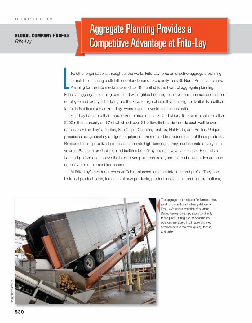
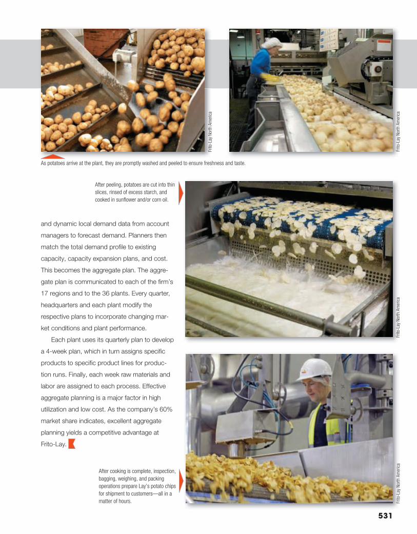
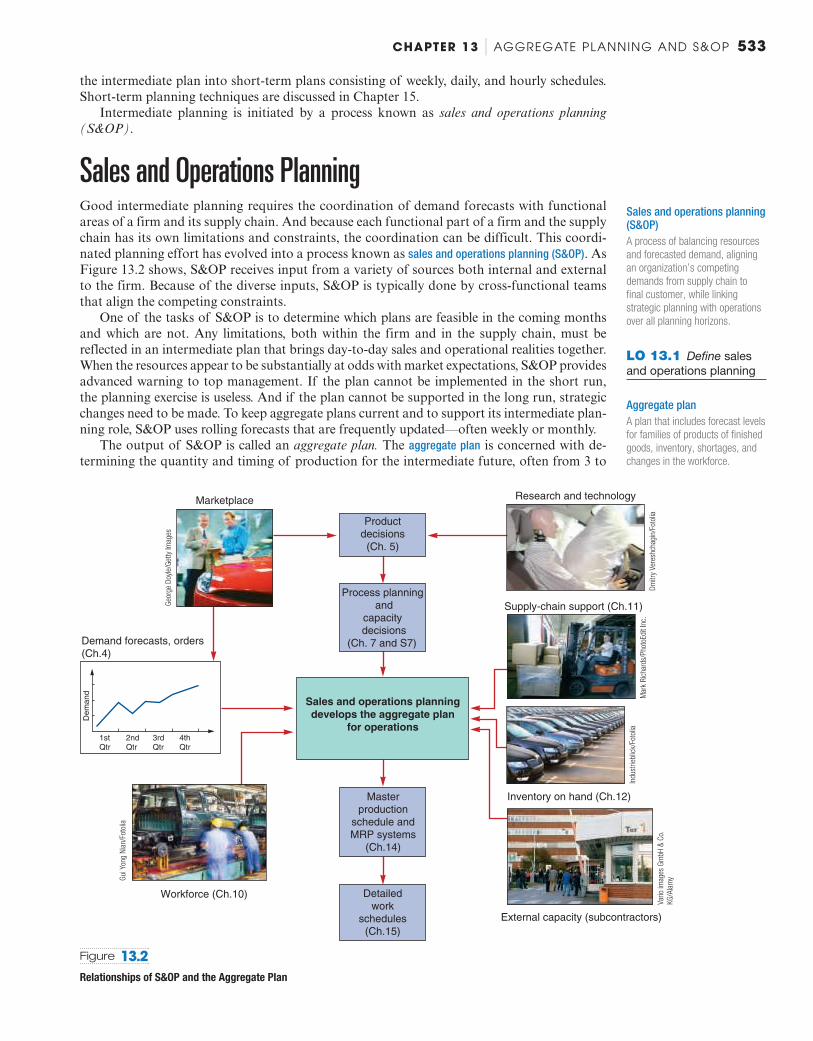
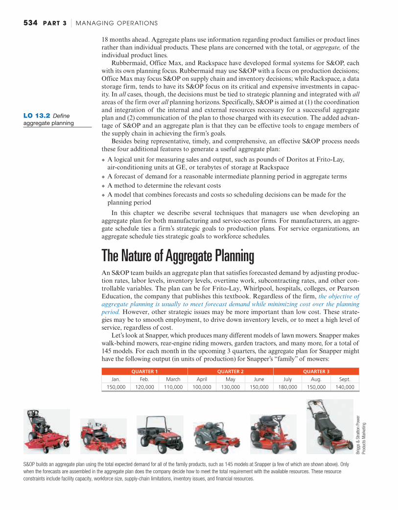
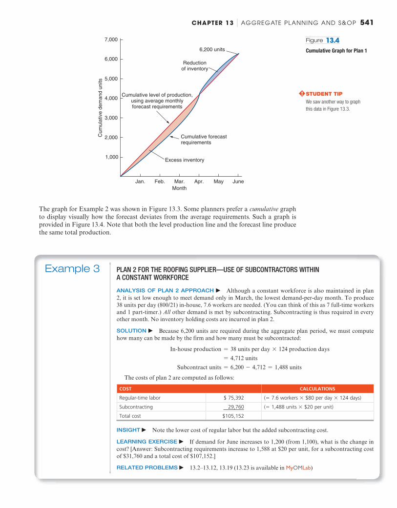
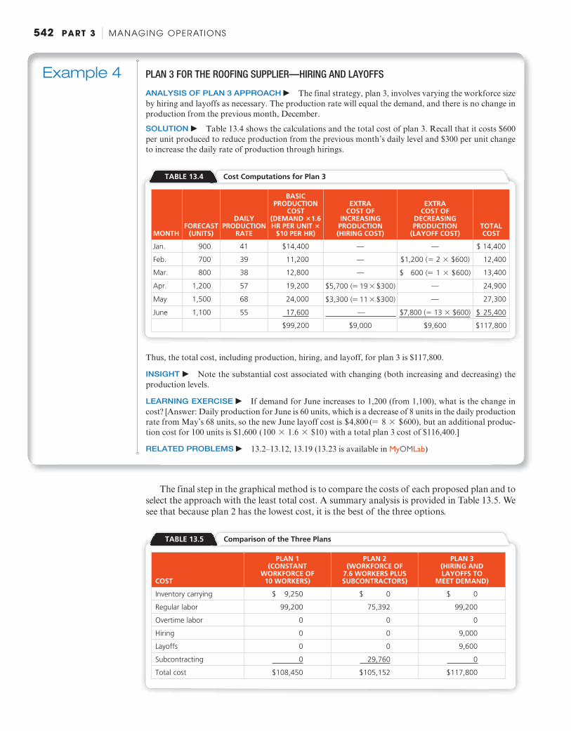
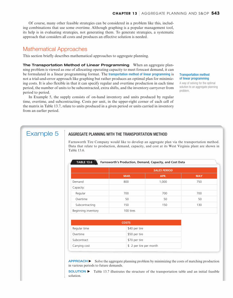
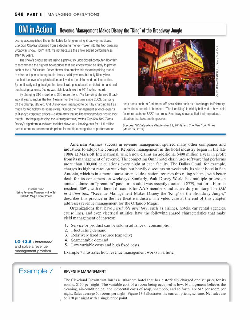
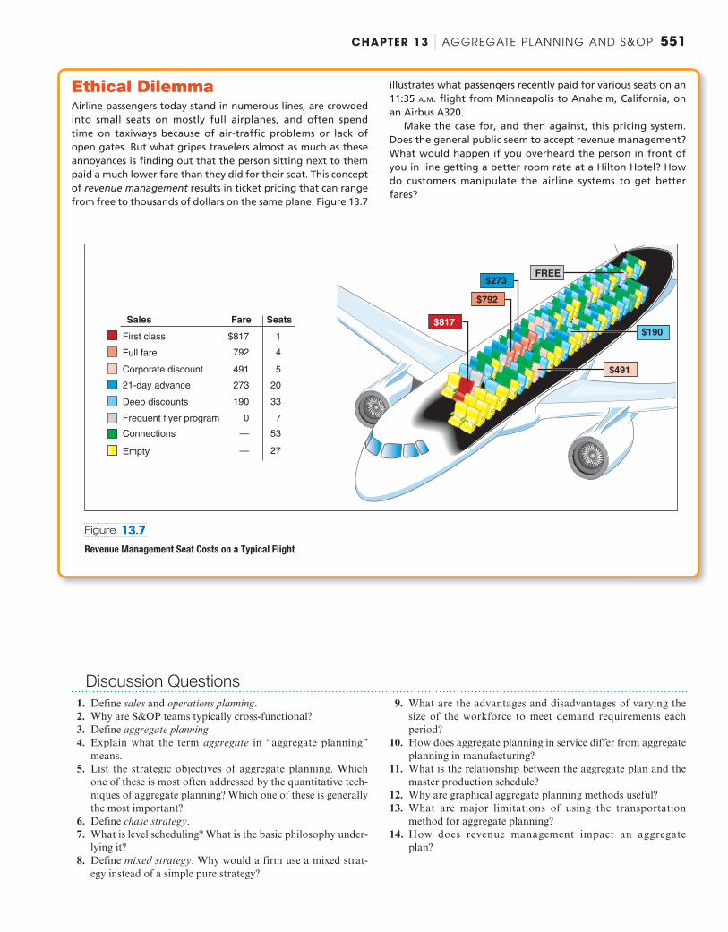
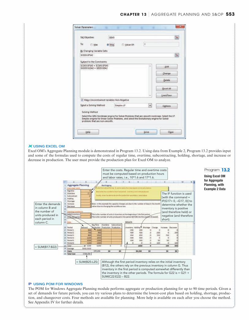
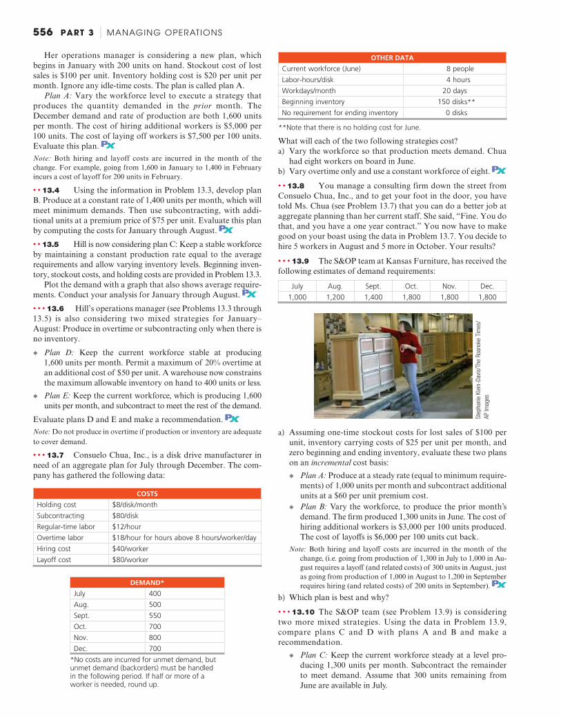
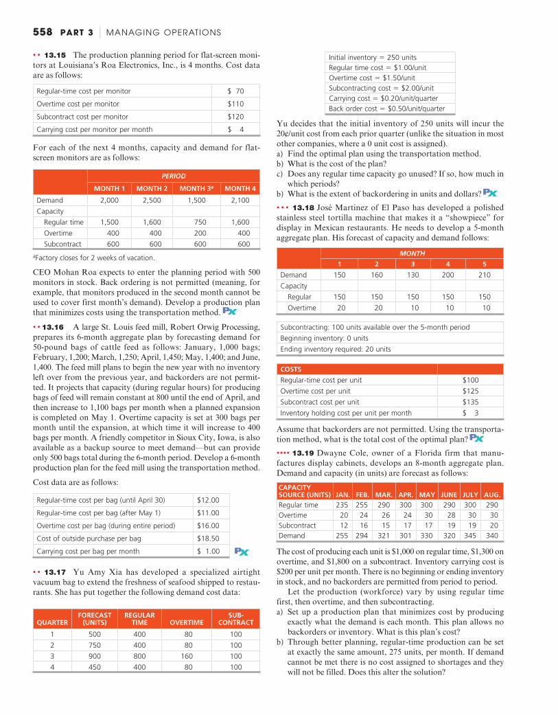

![[PPT]Production and Operations Management: …sureten/(aggregate planning)5.ppt · Web viewDisaggregating the Aggregate Plan Aggregate Planning Aggregate planning Intermediate-range](https://static.fdocuments.in/doc/165x107/5aec86827f8b9ab24d902697/pptproduction-and-operations-management-suretenaggregate-planning5pptweb.jpg)