Res. Lett. Inf. Math. Sci., 2003, Vol.5, pp 129-142Available online at http://iims.massey.ac.nz/research/letters/

129

Agglomerate Properties

P. R. Rynhart1 , J. R. Jones2 & R. McKibbin3

1 Institute of Fundamental SciencesMassey University, Palmerston North, New Zealand.

2 Institute of Technology & EngineeringMassey University, Palmerston North, New Zealand.3 Institute of Information & Mathematical Sciences

Massey University at Albany, Auckland, New Zealand.

Modelling of wet granulation requires the rate of agglomerate coalescence to be estimated.Coalescence is dependent on the frequency of collisions that occur, and the fraction of collisionswhich result in coalescence. The collision rate is a function of granulator kinetics and powderproperties, while the coalescence success rate is dependent on factors including the Stokesnumber and particle geometry. This work investigates an aspect of the geometry by examiningthe distribution of liquid on the surface of agglomerates in the capillary state. Agglomeratesare created by adding particles, one at a time, about a central tetrahedral arrangement offour primary particles. For a given agglomerate, the wetted fraction of surface area, definedas the wetness, is evaluated using an approximate fluid surface. Packing density and bindersaturation parameters are incorporated into the model. Given a number of primary particlesand the volume of binder in a particle, the agglomerate wetness is able to be estimated usingcomputational geometry.

1 INTRODUCTION

In granulation binder content and binder viscosity interact in complex ways, affecting the con-solidation rate and the final extent of consolidation (1). Granule growth is considered to be dueto coalescence and breakage, with a system eventually reaching an equilibrium state. Models ofgrowth regard granules as either rigid (2) or plastic (3), but these assume the presence of a continu-ous layer of liquid at the contact interface. The liquid acts to dissipate some of the collision energy.In plastic collisions, deformation further dissipates the collision energy. Simons and Fairbrother (4)define successful coalescence to have occurred when the rupture energy of a liquid bridge formedbetween granules is greater than the kinetic energy of impact. None of these models define a real-istic liquid surface for granules; instead they rely on assuming a smooth surfaced granule which iscovered by a binder of uniform thickness. Thorton and Ning (5) produce a granule with a pseudorealistic appearance, but use an adhesion energy rather than a liquid surface. Thus, there is a needto define a realistic agglomerate surface which is formed from both wet and dry regions. Duringconsolidation, the ratio of these wet to dry regions will change.

In this paper, a description of the algorithm for building agglomerates is detailed, where primaryparticles are added to the granule one at a time. This is analogous to the layering mechanism whereagglomerates increase in size primarily as the result of single primary particle contacts. Due tothe stochastic motion of particles in a granulator, primary particles are equally likely to collidewith an agglomerate from any direction, and hence the long term average is to produce granules

130 P. R. Rynhart, J. R. Jones & R. McKibbin

which are closely packed and spherical. The calculation of the binder fluid surface, along with therespective volume and surface area occupied by the primary particles and binder fluid, is discussedin a later section. In performing these calculations, the probability of agglomerate coalescence isable to be estimated.

In this model, agglomerates consist of primary particles (spheres) and binder fluid, where thefluid is formed by a union of tetrahedral segments. The starting configuration is the tetrahedralarrangement of 4 particles as illustrated in figure 59(a), and additional particles are added tothe agglomerate individually. As a new particle is added, fluid segments form between the newparticle and existing particles of the agglomerate. The minimum distance between sphere centresis defined by σ = 2R + s, where R is the radius of the equally sized primary particles and s isthe minimum separation between spheres. At a given stage in construction, a matrix S stores theCartesian coordinates of the primary particles as row vectors, and the fluid surface is defined bythree matrices, T , F and E. For each fluid segment, T stores the four vertices of the tetrahedrain terms of indices into S. Each row entry in F defines a fluid surface face, where the first threeentries of the row refer to the face vertices as indices into S. Additional information stored inan F entry is the outward pointing normal vector of the face, an estimate point for an additionalparticle (if the face is subsequently selected to bond to a new particle), and a flag as to whetherthe face is internal (1) or external (0). Faces become internal when a new particle bonds with theagglomerate, forming new external faces. An edge matrix E is also maintained; this matrix is usedfor viewing the agglomerate only, and is not involved in the algorithm for adding new particles.The estimate point for a new particle ei to be added to face fi is obtained from the geometricmid-point O of the three vertices on the face, and the minimum distance between spheres σ. Thisyields an estimate point for the added particles O+niH, where x is the distance from a face vertexto the midpoint, ni is the normal vector and H is the estimated height above the face,

√σ2 − x2.

In the initial case shown in figure 59(a), matrices T , F and E appear as follows ;

T4 =[

1 2 3 4], F4 =

1 2 3 n1 e1 11 3 4 n2 e2 11 2 4 n3 e3 12 3 4 n4 e4 1

, E4 =

1 21 31 42 32 43 4

,

where ni is the outward pointing normal vector of face i, ei is the estimate point for a new particleon face i, and the final column of F indicates that all faces are external for the initial arrangement.The subscript N on the T , F and E matrices refer to the matrices for an N particle agglomerate.

When adding a fifth particle to face with index 1 (face [1 2 3]), a new tetrahedron is added,face 1 becomes internal, and 3 faces and 3 edges are added. Figure 59 shows the original (orbase) tetrahedron for the 4 particle case on the left, and the 5 particle case is shown on the right.Following the addition of the 5th particle, matrices T , F , and E are updated as follows ;

T5 =[

1 2 3 42 3 4 5

], F5 =

1 2 3 n1 e1 01 3 4 n2 e2 11 2 4 n3 e3 12 3 4 n4 e4 15 1 2 n5 e5 15 1 3 n6 e6 15 2 3 n7 e7 1

, E5 =

1 21 31 43 42 32 41 52 53 5

.

Agglomerate Properties 131

Figure 59: The tetrahedron on the left defines placement of the spheres for primary particles 1-4.When a 5th particle is added, the arrangement is given by the 2 tetrahedra (as on the right).

2 AGGLOMERATE GROWTH ALGORITHM

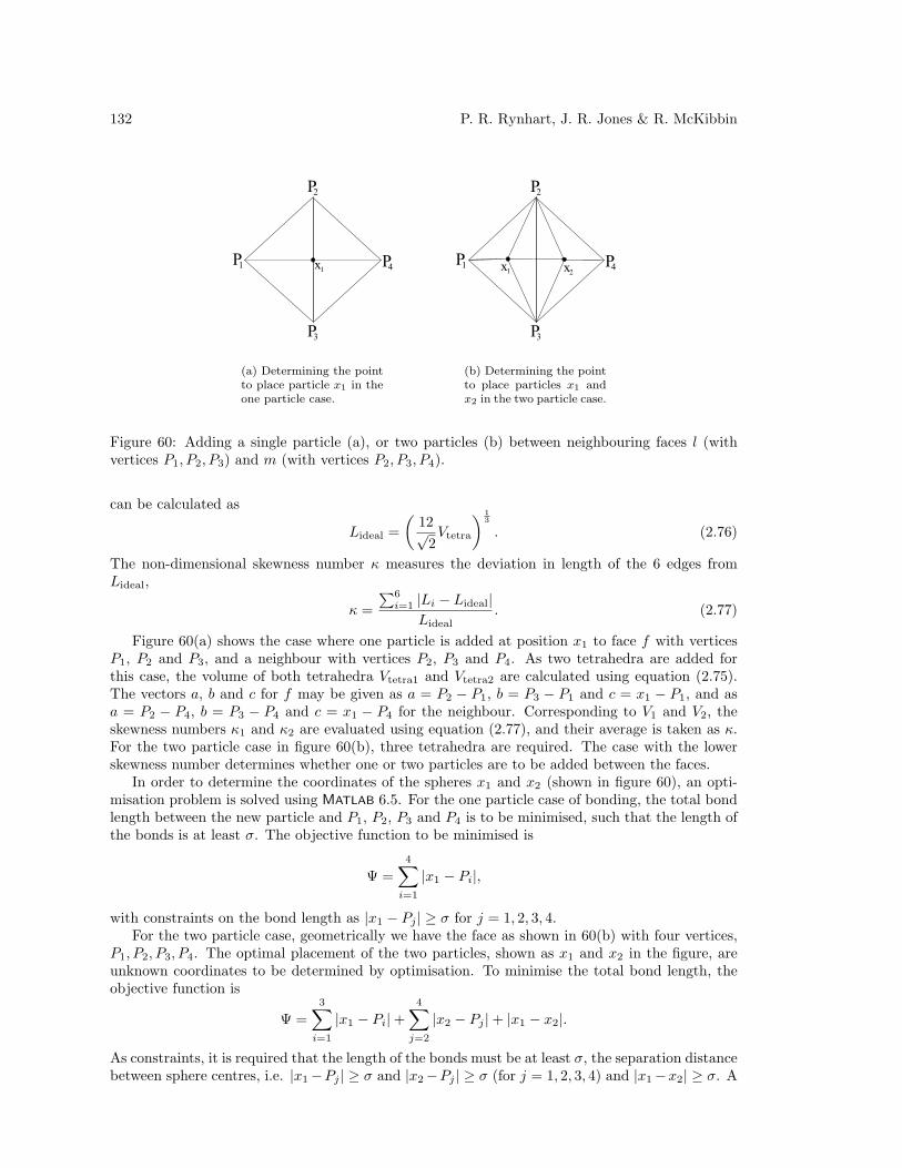
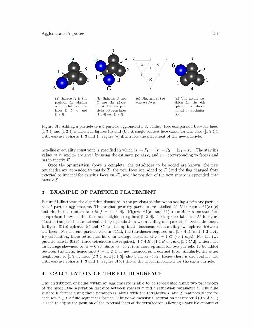
Agglomerates grow by adding particles to an existing agglomerate. To maintain spherical growthbehaviour, the incoming particle approaches the first external face f ∈ F , as this is approximatelythe closest external face to the centre of the agglomerate. In the simple case where the additionof a particle results in the formation of one new tetrahedra, the coordinates of the new particleare given by the estimate position for face f , ei. In more complex cases, the incoming particleforms contact with more than one face, resulting in more than one tetrahedra. The new particleposition is then given by the solution to an optimisation problem which is discussed later. Testswith all neighbouring faces of f are used to determine how many tetrahedra are to be added asa result of the new particle. The test consists of two scenarios which are compared on the basisof the regularity of the resulting tetrahedra. The first scenario, illustrated in figure 60(a), placesthe new particle between face f and the neighbour creating two tetrahedra. The average skewnessof the tetrahedra is calculated using the method discussed below. The second scenario shown infigure 60(b) positions two particles between the faces, resulting in three tetrahedra and the averageskewness is again calculated. If the average skewness of scenario two is lower than that of one forall neighbouring faces to f , i.e. if it is more optimal to place two particles between f and itsneighbours, then only one new tetrahedra is formed and the particle is placed in position ei. Anexample of this case is shown in figure 61. If the skewness in scenario one is lower for any pair inthe test, then the neighbour to f is added as a face which will bond with the new particle. Thisneighbouring face then tests its own neighbours pairwise (excluding the parent) using the skewnesscriteria, which may result in additional faces that bond with the new particle. The set of faces thatbond with the new particle are known as contact faces, and form the bases of the new tetrahedrawhich are to be added. Spheres which share their vertices with the contact faces, and which bondwith the new particle, are known as contact spheres.

A quantity called the skewness number κ is introduced to test the regularity of added tetrahedra.This number measures how much a proposed tetrahedron with volume Vtetra deviates from a regular(or ideal) tetrahedron of the same volume. A regular tetrahedron has κ = 0, with larger skewnessnumbers implying that the given tetrahedron deviates more strongly from the ideal shape. Thevolume of the given tetrahedron is calculated using

Vtetra =16|a · b× c| (2.75)

where a, b, c are vectors from one vertex of the new tetrahedron to the other vertices. Using theequation for the volume of a regular tetrahedron, the ideal edge length (of a regular tetrahedron)

132 P. R. Rynhart, J. R. Jones & R. McKibbin

(a) Determining the pointto place particle x1 in theone particle case.

(b) Determining the pointto place particles x1 andx2 in the two particle case.

Figure 60: Adding a single particle (a), or two particles (b) between neighbouring faces l (withvertices P1, P2, P3) and m (with vertices P2, P3, P4).

can be calculated as

Lideal =(

12√2Vtetra

) 13

. (2.76)

The non-dimensional skewness number κ measures the deviation in length of the 6 edges fromLideal,

κ =∑6

i=1 |Li − Lideal|Lideal

. (2.77)

Figure 60(a) shows the case where one particle is added at position x1 to face f with verticesP1, P2 and P3, and a neighbour with vertices P2, P3 and P4. As two tetrahedra are added forthis case, the volume of both tetrahedra Vtetra1 and Vtetra2 are calculated using equation (2.75).The vectors a, b and c for f may be given as a = P2 − P1, b = P3 − P1 and c = x1 − P1, and asa = P2 − P4, b = P3 − P4 and c = x1 − P4 for the neighbour. Corresponding to V1 and V2, theskewness numbers κ1 and κ2 are evaluated using equation (2.77), and their average is taken as κ.For the two particle case in figure 60(b), three tetrahedra are required. The case with the lowerskewness number determines whether one or two particles are to be added between the faces.

In order to determine the coordinates of the spheres x1 and x2 (shown in figure 60), an opti-misation problem is solved using MATLAB 6.5. For the one particle case of bonding, the total bondlength between the new particle and P1, P2, P3 and P4 is to be minimised, such that the length ofthe bonds is at least σ. The objective function to be minimised is

Ψ =4∑

i=1

|x1 − Pi|,

with constraints on the bond length as |x1 − Pj | ≥ σ for j = 1, 2, 3, 4.For the two particle case, geometrically we have the face as shown in 60(b) with four vertices,

P1, P2, P3, P4. The optimal placement of the two particles, shown as x1 and x2 in the figure, areunknown coordinates to be determined by optimisation. To minimise the total bond length, theobjective function is

Ψ =3∑

i=1

|x1 − Pi|+4∑

j=2

|x2 − Pj |+ |x1 − x2|.

As constraints, it is required that the length of the bonds must be at least σ, the separation distancebetween sphere centres, i.e. |x1−Pj | ≥ σ and |x2−Pj | ≥ σ (for j = 1, 2, 3, 4) and |x1−x2| ≥ σ. A

Agglomerate Properties 133

(a) Sphere A is theposition for placingone particle betweenfaces [1 3 4] and[1 2 4].

(b) Spheres B andC are the place-ment for two par-ticles between faces[1 3 4] and [1 2 4].

(c) Diagram of thecontact faces.

(d) The actual po-sition for the 6thsphere, as deter-mined by optimisa-tion.

Figure 61: Adding a particle to a 5 particle agglomerate. A contact face comparison between faces[1 3 4] and [1 2 4] is shown in figures (a) and (b). A single contact face exists for this case ([1 3 4]),with contact spheres 1, 3 and 4. Figure (c) illustrates the placement of the new particle.

non-linear equality constraint is specified in which |xi − P1| = |xj − P4| = |x1 − x2|. The startingvalues of x1 and x2 are given by using the estimate points el and em (corresponding to faces l andm) in matrix F .

Once the optimisation above is complete, the tetrahedra to be added are known; the newtetrahedra are appended to matrix T , the new faces are added to F (and the flag changed fromexternal to internal for existing faces on F ), and the position of the new sphere is appended ontomatrix S.

3 EXAMPLE OF PARTICLE PLACEMENT

Figure 61 illustrates the algorithm discussed in the previous section when adding a primary particleto a 5 particle agglomerate. The original primary particles are labelled ‘1’-‘5’ in figures 61(a)-(c)and the initial contact face is f = [1 3 4]. Figures 61(a) and 61(b) consider a contact facecomparison between this face and neighbouring face [1 2 4]. The sphere labelled ‘A’ in figure61(a) is the position as determined by optimisation when adding one particle between the faces.In figure 61(b) spheres ‘B’ and ‘C’ are the optimal placement when adding two spheres betweenthe faces. For the one particle case in 61(a), the tetrahedra required are [1 3 4 A] and [1 2 4 A].By calculation, these tetrahedra have an average skewness of κ1 = 1.83 (to 2 d.p.). For the twoparticle case in 61(b), three tetrahedra are required, [1 3 4 B], [1 4 B C], and [1 4 C 2], which havean average skewness of κ2 = 0.36. Since κ2 < κ1, it is more optimal for two particles to be addedbetween the faces, hence face f = [1 2 4] is not included as a contact face. Similarly, the otherneighbours to [1 3 4], faces [2 3 4] and [5 1 3], also yield κ2 < κ1. Hence there is one contact facewith contact spheres 1, 3 and 4. Figure 61(d) shows the actual placement for the sixth particle.

4 CALCULATION OF THE FLUID SURFACE

The distribution of liquid within an agglomerate is able to be represented using two parametersof the model, the separation distance between spheres σ and a saturation parameter δ. The fluidsurface is formed using these parameters, along with the tetrahedra T and S matrices where foreach row t ∈ T a fluid segment is formed. The non-dimensional saturation parameter δ (0 ≤ δ ≤ 1)is used to adjust the position of the external faces of the tetrahedron, allowing a variable amount of

134 P. R. Rynhart, J. R. Jones & R. McKibbin

(a) The unex-panded bindertetrahedra, cor-responding toδ = 0

(b) Fluid tetrahe-dra, expanded byδ = 0.7.

(c) Cylinders addedto saturation stateδ = 0.7.

(d) Half-space cutsare used to producean object which isclosed off.

Figure 62: Creation of a binder fluid segment

volume to exist within the agglomerate. The state δ = 0 corresponds to a non-expanded state, inwhich the fluid surface is connected to the centres of the primary particles. For higher saturationstates, δ > 0, the fluid surface is defined by moving the external faces of the tetrahedron in thedirection of their outward pointing normal vectors, up to a maximum saturation state of δ = 1. Asaturation of δ = 1 corresponds to the case where the faces are moved outward a distance R equalto the radius of the spheres. Figure 62(a) shows the unexpanded state δ = 0, while figure 62(b)illustrates the saturation state δ = 0.7. The location of the primary particles remain fixed as thesaturation state is varied; the points ‘+’ shown in figure 62 correspond to the centre points of theprimary particles. In all but the δ = 0 case, cylinders of radius δ connect adjacent faces togetheralong the edges of the tetrahedron as shown in figure 62(c). k points along each of the cylinderslink adjacent faces of the tetrahedron together. Triangular mapping is used to form the verticesand faces of the cylinders. The value of k is called the polyhedra accuracy. Once the cylinders areadded, the first derivative of the surface is continuous, but discontinuities in the second derivativeoccur where cylinders intersect with the faces of the tetrahedron. As a result the fluid segmentsdo not have constant mean curvature, and therefore the fluid surface is an approximation to thetrue binder surface.

As discussed in section 5, the binder fluid segments Ti must be convex objects. This is achievedby forming the object as above, and then closing off the object by intersecting with planes thatpass through the lowest points of the expanded faces (the points 1, 2 and 3 in figures 62(b) and62(c)). The completed binder segment is shown in figure 62(d).

5 AGGLOMERATE PROPERTIES

In this section, some concepts are introduced which enable agglomerate properties, which includethe surface area, volume, and fraction of wetted surface area, to be evaluated. An agglomerate isthe non-convex union of nS primary particles with nT tetrahedra, or

(nS⋃i=1

Si) ∪ (nT⋃i=1

Ti). (5.78)

Although these properties can only be evaluated for convex objects, the non-convex union inequation (5.78) can be written in terms of convex sets. This is achieved by taking unions anddifferences of the convex sets Si and Ti (as unions and differences of convex sets are also convex).Convex sets are able to be written as a collection of half-spaces; a half-space is defined as

n · (x− x0) ≤ 0 (n 6= 0), (5.79)

Agglomerate Properties 135

where n ∈ R3 is an outward pointing normal vector and x0 ∈ R3 is a point that lies on the plane

n · (x− x0) = 0 (n 6= 0). (5.80)

It is common to define d = n · x0. Using d, equation (5.79) is written

n · x ≤ d (n 6= 0). (5.81)

A polyhedron is a bounded convex set formed by the intersection of a finite number of half-spaces; the spheres Si are polyhedra, and the construction of the Ti objects (discussed in section4) is such that the fluid segments are polyhedra. As a half-space is convex, and since intersectionsbetween convex regions are convex, polyhedra are convex. Properties of polyhedra including thesurface area and volume can be calculated. In general, the volume of non-convex objects can onlybe evaluated by first dividing the object into convex regions, and summing properties of the convexportions piecewise. For a union of convex components Ai,⋃

i

Ai =∑

i

Ai −∑i 6=j

Ai ∩Aj +∑

i 6=j 6=k

Ai ∩Aj ∩Ak − . . .±⋂i

Ai. (5.82)

Since polyhedra are an intersection of half-spaces, the intersection of two or more overlappingpolyhedra is also a polyhedra. The union in equation (5.82) requires polyhedra intersections to beevaluated.

Construction of the agglomerate (sphere placement, binder fluid placement, and matrices S,T and F ) are completed using MATLAB . Computational geometry calculations were completedusing an external C++ mathematics library written by Jonathan Marshall3. The library includesroutines to calculate the intersection between two polyhedra (e.g. P1 and P2 producing P1 ∩ P2),the intersection of a polyhedra P with a half-space, and the calculation of area and volume ofpolyhedra.

6 CALCULATING SURFACE AREA, VOLUME AND THE WET-NESS

The wetness W is defined as the wetted fraction of the exterior agglomerate surface area. As Wis the fraction of binder fluid accessible to other incident particles, it is proposed that when twoagglomerates collide the probability of coalescence is related to the wetness of both agglomerates.Exactly how the agglomerate wetness relates to coalescence is not examined in this paper.

The wetness of agglomerates is calculated using variables Awet and Adry which refer to wet anddry surface areas of the particle. Primary particles drawn on the binder surface of figure 62(d) areshown in figure 63(a). In this figure, the total agglomerate surface area A = Adry + Awet is thesum of the exposed surface area of the spheres and the binder fluid. For the 4 particle case, thepolyhedra that result from the intersection of the primary particles and binder fluid are shown infigure 63(b). Awet is calculated as the area of the binder less the area of the intersected polyhedracommon to the binder, and Adry is equal to the area of the spheres less the area of the intersectedpolyhedra common to the spheres. The wetness W is equal to

W =Awet

Awet +Adry. (6.83)

The primary particles of a 4 particle agglomerate are drawn in figure 63(a), along with the fluidtetrahedron T1. Dry regions are the sphere portions (where they do not overlap with the fluid),and the binder tetrahedron is wet (where it does not overlap with the spheres). Later, the wetnessis plotted as a function of the volume ratio of binder fluid to solids. The solids volume is simply

3Institute of Fundamental Sciences, Massey University, New Zealand

136 P. R. Rynhart, J. R. Jones & R. McKibbin

(a) A 4 particle agglom-erate, showing placementof primary particles andbinder fluid.

(b) Polyhedra resulting from theintersection between primary par-ticles and binder fluid.

Figure 63: In figure 63(a), primary particles and the binder tetrahedra is drawn. Figure 63(b)shows the intersected portions, obtained by intersecting the spheres with the binder fluid. For thisfigure, R = 1, δ = 0.7 and s = 0.5.

N × 43πR

3, and the binder volume Vwet is calculated using the volume of the tetrahedra and thevolume of the intersected regions such that (for the 4 particle case in figure 63)

Vwet = V (T1)−4∑

i=1

V (Si ∩ T1)

where V (P ) is the volume of polyhedron P . The fluids to solids ratio between Vwet and the volumeof solid is denoted V ∗. For the surface areas, Adry and Awet are

Awet = A(T1)−4∑

i=1

Awet(Si ∩ T1) and Adry =4∑

i=1

[A(Si)−Adry(Si ∩ T1)] (6.84)

where Adry(Si∩T1) is the area of Si∩T1 (see figure 63(b)) common to Si, and Awet(Si∩T1) is thearea of Si ∩ T1 (see figure 63(b)) common to T1. The wetness is calculated using equation (6.83).

7 CUTTING THE TETRAHEDRA

For saturation states δ > 0 neighbouring tetrahedra overlap when formed using the method ofsection 4. For large agglomerates, large number of overlaps occur between the tetrahedra andthe primary particles. Figure 64(a), for example, shows the 5 particle case where overlap occursbetween 2 fluid tetrahedra. The number of intersections required to calculate the union of equation(5.78) (as implied by equation (5.82)) are able to be minimised if overlap is not permitted betweenthe fluid segments, i.e. if Ti ∩ Tj = ∅ for i 6= j. If this is enforced, then since Si ∩ Sj = ∅ for i 6= j,then the only non-empty intersections are Si ∩Tj . This reduces the agglomerate union of equation(5.78) to ∑

i

Si +∑

i

Ti −∑i 6=j

Si ∩ Tj . (7.85)

Therefore, when adding a tetrahedron Tk, existing tetrahedra which neighbour Tk along with Tk

are cut to avoid overlap. Depending on how many vertices are shared between indices of Tk andthe neighbour, different half-space cuts are completed. If a face is shared with 3 common (primary

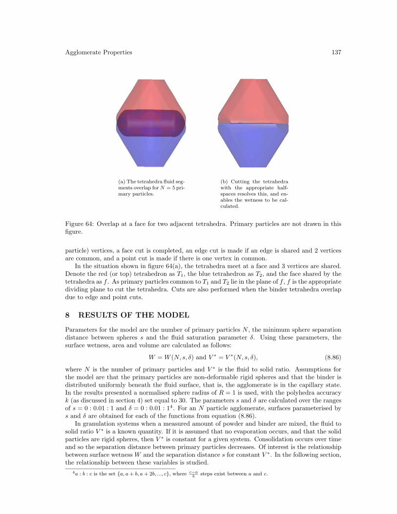
Agglomerate Properties 137

(a) The tetrahedra fluid seg-ments overlap for N = 5 pri-mary particles.

(b) Cutting the tetrahedrawith the appropriate half-spaces resolves this, and en-ables the wetness to be cal-culated.

Figure 64: Overlap at a face for two adjacent tetrahedra. Primary particles are not drawn in thisfigure.

particle) vertices, a face cut is completed, an edge cut is made if an edge is shared and 2 verticesare common, and a point cut is made if there is one vertex in common.

In the situation shown in figure 64(a), the tetrahedra meet at a face and 3 vertices are shared.Denote the red (or top) tetrahedron as T1, the blue tetrahedron as T2, and the face shared by thetetrahedra as f . As primary particles common to T1 and T2 lie in the plane of f , f is the appropriatedividing plane to cut the tetrahedra. Cuts are also performed when the binder tetrahedra overlapdue to edge and point cuts.

8 RESULTS OF THE MODEL

Parameters for the model are the number of primary particles N , the minimum sphere separationdistance between spheres s and the fluid saturation parameter δ. Using these parameters, thesurface wetness, area and volume are calculated as follows:

W = W (N, s, δ) and V ∗ = V ∗(N, s, δ), (8.86)

where N is the number of primary particles and V ∗ is the fluid to solid ratio. Assumptions forthe model are that the primary particles are non-deformable rigid spheres and that the binder isdistributed uniformly beneath the fluid surface, that is, the agglomerate is in the capillary state.In the results presented a normalised sphere radius of R = 1 is used, with the polyhedra accuracyk (as discussed in section 4) set equal to 30. The parameters s and δ are calculated over the rangesof s = 0 : 0.01 : 1 and δ = 0 : 0.01 : 14. For an N particle agglomerate, surfaces parameterised bys and δ are obtained for each of the functions from equation (8.86).

In granulation systems when a measured amount of powder and binder are mixed, the fluid tosolid ratio V ∗ is a known quantity. If it is assumed that no evaporation occurs, and that the solidparticles are rigid spheres, then V ∗ is constant for a given system. Consolidation occurs over timeand so the separation distance between primary particles decreases. Of interest is the relationshipbetween surface wetness W and the separation distance s for constant V ∗. In the following section,the relationship between these variables is studied.

4a : b : c is the set {a, a + b, a + 2b, ..., c}, where c−ab

steps exist between a and c.

138 P. R. Rynhart, J. R. Jones & R. McKibbin

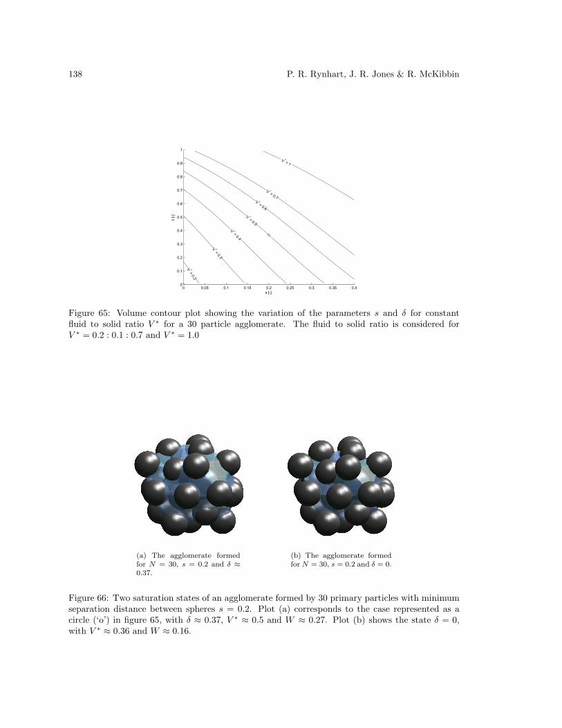
Figure 65: Volume contour plot showing the variation of the parameters s and δ for constantfluid to solid ratio V ∗ for a 30 particle agglomerate. The fluid to solid ratio is considered forV ∗ = 0.2 : 0.1 : 0.7 and V ∗ = 1.0

(a) The agglomerate formedfor N = 30, s = 0.2 and δ ≈0.37.

(b) The agglomerate formedfor N = 30, s = 0.2 and δ = 0.

Figure 66: Two saturation states of an agglomerate formed by 30 primary particles with minimumseparation distance between spheres s = 0.2. Plot (a) corresponds to the case represented as acircle (‘o’) in figure 65, with δ ≈ 0.37, V ∗ ≈ 0.5 and W ≈ 0.27. Plot (b) shows the state δ = 0,with V ∗ ≈ 0.36 and W ≈ 0.16.

Agglomerate Properties 139

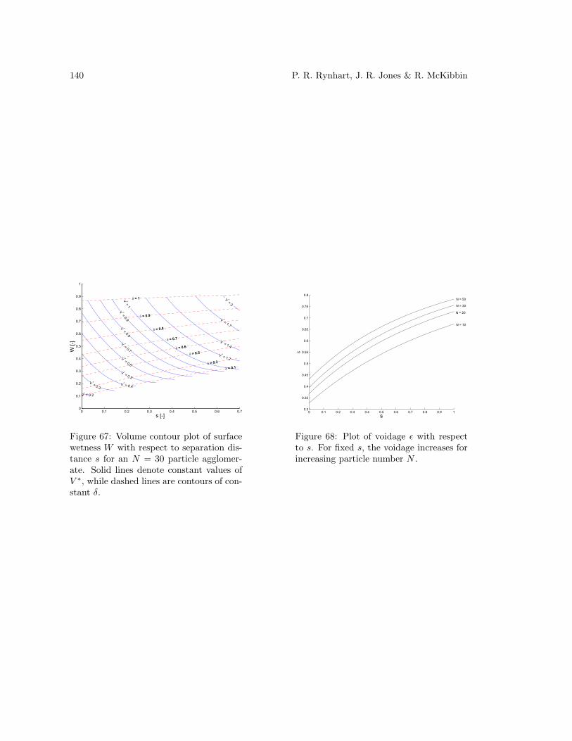
9 SURFACE WETNESS ANALYSIS

The mechanism by which consolidation occurs has been studied by workers including (3), butis not considered in this study. Given that agglomerates consolidate, this work investigates thechange in surface wetness W that results from a decrease in the inter-particle separation distances. The relationship between s and δ for fixed values of the fluid to solid ratio V ∗ for a 30 particleagglomerate is shown in figure 65 for V ∗ = 0.2 : 0.1 : 0.7 and V ∗ = 1.0. A particular agglomer-ate is defined by fixing three of the parameters of the model; the complete set of parameters isW,A∗, V ∗, N, δ and s. An example is given in figure 66(a), where the fixed parameters are N = 30,s = 0.2 and V ∗ = 0.5. In the contour plot of figure 65, this configuration is shown as a circle(‘o’) on the V ∗ = 0.5 contour. Using the functions V ∗ and W , the liquid saturation state for thisexample is δ ≈ 0.37 and the surface wetness is W ≈ 0.27, implying that approximately 27% ofthe agglomerate is surface wet. For a fixed inter-particle separation distance, the surface wetnessincreases with increasing fluid to solid ratio V ∗, which agrees with intuition.

Figure 67 shows a plot of surface wetness W with respect to separation distance s for a rangeof V ∗ values. Dashed contours on this figure represent constant values of the liquid saturationparameter δ. The figure shows that for decreasing separation distance s, an increase in the surfacewetness W occurs for constant V ∗. This can be understood by considering an N particle agglom-erate in a expanded (or loosely-packed) state, with separation distance s1. When consolidationoccurs, and the separation distance is decreased from s1 to s2, the void volume of the agglomeratereduces. This forces the fluid to migrate from the interior of the particle to the agglomerate surface,which has the effect of increasing the surface wetness.

Figure 69 shows the trend of surface wetness with respect to inter-particle separation distancefor different sized agglomerates; in particular for N = 10, 20, 30 and 50. Several different values ofthe fluid to solid ratio V ∗ are shown in each of the plots of 69(a)-69(d). For fixed N , the surfacewetness increases for decreasing separation distance s, as discussed above. For fixed inter-particleseparation distance s, and for a particular V ∗, the figure shows decreasing surface wetness forincreasing numbers of primary particles (N). This behaviour can be explained by introducing thecommonly used voidage ε, which is defined, for the maximal saturation state δ = 1, as

ε =Vwet

Vwet +N × 43πR

3, (9.87)

where Vliquid is the volume of binder fluid in an agglomerate normalised to the volume of a primaryparticle, and Vsolid is equal to N (as Vliquid and Vsolid are normalised to the volume of a sphereof radius R). The voidage calculation given in equation (9.87) is akin to ‘wrapping’ the surfaceof the particle with cellophane, and then calculating the fraction of volume occupied by liquid.Figure 68 shows the relationship between voidage and the inter-particle separation distance s,which shows that, for fixed s, voidage ε increases with increasing N . As more particles are addedto the agglomerate (increasing the radius of the particle), more void space is introduced. The resultshown in figure 68 suggests that the void (internal) volume increases as the particle increases inradius. As there is proportionally more volume interior to the agglomerate, more binder fluid existsinside the particle and this reduces the surface wetness of the agglomerate. Figure 70 considersthe relationship plotted in figure 67 for varied number of primary particles N . In general, forconstant V ∗, this figure shows that small agglomerates are the most surface wet with surfacewetness decreasing as more primary particles are added.

The contours of wetness in figures 67 and 69 have an upper limit with respect to W due theidealised model described in section 4, where saturation has a maximum value of δ = 1. In reality,for such super-saturated states (i.e. for δ > 1) the fluid would completely enclose the primaryparticles to form a slurry, but this is of no interest in granulation. Conversely, for dry particles,the wetness may be less than those given in figure 67 which correspond to δ = 0. The value δ = 0is not a physical limit, but is a model limit due to the methods described in section 4 to constructthe binder surface.

140 P. R. Rynhart, J. R. Jones & R. McKibbin

Figure 67: Volume contour plot of surfacewetness W with respect to separation dis-tance s for an N = 30 particle agglomer-ate. Solid lines denote constant values ofV ∗, while dashed lines are contours of con-stant δ.

Figure 68: Plot of voidage ε with respectto s. For fixed s, the voidage increases forincreasing particle number N .

Agglomerate Properties 141

(a) V ∗ = 0.3 (b) V ∗ = 0.5

(c) V ∗ = 0.7 (d) V ∗ = 1.0

Figure 69: Plot of surface wetness W with respect to inter-particle separationdistance s for agglomerates composed of 10, 20, 30 and 50 primary particles.Values of V ∗ used in this figure are V = 0.3, 0.5, 0.7 and 1.0.

(a) s = 0 (b) s = 0.2

(c) s = 0.5 (d) s = 0.7

Figure 70: Graphs of wetness W with respect to particle number N for a rangeof s and a range of fluids to solid ratio values V ∗.

142

10 CONCLUSIONS

The following conclusions can be drawn from this model about surface wetness as a function ofthe number of primary particles in the agglomerate, the separation distance of these particles, andthe saturation of the agglomerate.

• small agglomerates are the most surface wet for a constant separation distance, and largeagglomerates have a lower surface wetness.

• as the separation distance decreases during consolidation, and for constant values of the fluidsto solids volume ratio V ∗ the, wetness increases.

• the rate of change of wetness increases with further consolidation.

• agglomerates with larger fluids to solids volume ratio have greater surface wetness.

11 ACKNOWLEDGEMENT

The authors wish to thank Jonathan Marshall, Institute of Fundamental Sciences, Massey Univer-sity, for developing the computational geometry toolbox used in this project. A short descriptionof the routines used was discussed in section 5.

References

[1] Simon M. Iveson, James D. Litster, Karen Hapgood and Bryan J. Ennis. Nucleation, growthand breakage phenomena in agitated wet granulation processes: a review. Powder Technology,117:3–39, 2001.

[2] B.J. Ennis, G.I. Tardos, R. Pfeffer. A microlevel based characterisation of granulation phe-nomena. Powder Technology, 65:257–272, 1991.

[3] L.X. Liu, J.D. Litster, S.M. Iveson, B.J. Ennis. Coalescence of deformable granules in wetgranulation processes. American Institute of Chemical Engineers, 46:529–539, 2000.

[4] S.J.R. Simons and R.J. Fairbrother. Direct observations of liquid binder-particle interactions:the role of wetting behaviour in agglomerate growth. Powder Technology, 110:44–58, 2000.

[5] C. Thornton and Z. Ning. A theorectical model for the stick/bounce behaviour of adhesive,elastic-plastic spheres. Powder Technology, 99:154–162, 1998.