Agent-Based Simulator for the German Electricity Wholesale ... · Agent-Based Simulator for the...

Semester Project:

Agent-Based Simulator for the German Electricity

Wholesale Market Including Wind Power

Generation and Widescale PHEV Adoption

Author: Lukas A. WehingerSupervisor: Matthias David Galus

Expert: Prof. Goran AnderssonTutor: Prof. Thomas Rutherford

Fall semester 2009February 5, 2010

Contents

Abstract iii

Symbols iv

1 Introduction and Contribution of the Semester Thesis 2

2 Agent-Based Modeling and Learning Algorithms: The LCS Ap-proach 52.1 Multi-Agent Modeling and Reinforcement Learning . . . . . . . . . . 52.2 The XCS Classifier System . . . . . . . . . . . . . . . . . . . . . . . 7

2.2.1 The Genetic Algorithm of XCS . . . . . . . . . . . . . . . . . 8

3 Modeling an Electricity Market with an Agent-Based Methodol-ogy 113.1 Concepts for Electricity Market Models . . . . . . . . . . . . . . . . 113.2 Why Using a Multi-Agent Approach in Electricity Markets? . . . . . 113.3 Methodology for a Multi-Agent Approach in Electricity Markets . . 12

3.3.1 Market Participants and Input Data . . . . . . . . . . . . . . 123.3.2 Action Sets, Market Structure and Clearing . . . . . . . . . . 133.3.3 Calculation of the Variable Cost of Production . . . . . . . . 143.3.4 Generator and Utility Reward Calculation . . . . . . . . . . . 15

4 Model Application: The German Electricity Market 164.1 The German Electricity Market . . . . . . . . . . . . . . . . . . . . . 164.2 Simplifications of the Model . . . . . . . . . . . . . . . . . . . . . . . 174.3 Market Participants . . . . . . . . . . . . . . . . . . . . . . . . . . . 174.4 Data Specification . . . . . . . . . . . . . . . . . . . . . . . . . . . . 184.5 Graphical Representation of the Single Processes by the Agent-Based

Model . . . . . . . . . . . . . . . . . . . . . . . . . . . . . . . . . . . 19

5 Results of the Simulation under Reference Condition 255.1 Results After the Basis Year . . . . . . . . . . . . . . . . . . . . . . . 255.2 Results after a Learning Interval . . . . . . . . . . . . . . . . . . . . 26

5.2.1 Spot Market Price Analysis . . . . . . . . . . . . . . . . . . . 265.2.2 The Bidding Behavior of the Agents . . . . . . . . . . . . . . 295.2.3 Profit of the Utilities . . . . . . . . . . . . . . . . . . . . . . . 31

6 Scenario Analysis 326.1 Scenarios with an Increased Wind Energy Contribution . . . . . . . 326.2 Scenarios with a Storage Device . . . . . . . . . . . . . . . . . . . . . 34

6.2.1 Charging Plug-ins With a Given Loading Distribution: Sce-nario one . . . . . . . . . . . . . . . . . . . . . . . . . . . . . 35

6.2.2 Charging Plug-ins During Off-Peak Hours: Scenario two . . . 37

i

6.2.3 Introducing Plug-ins with Spot Market Price Sensitive Charg-ing Characteristic: Scenario three . . . . . . . . . . . . . . . . 40

6.2.4 Introducing Plug-ins with Spot Market Price Sensitive Charg-ing Characteristic and Increased Wind Contribution: Sce-nario four . . . . . . . . . . . . . . . . . . . . . . . . . . . . . 43

7 Conclusion 44

ii

Abstract

The deregulation in electricity markets has led to substantial changes. The genera-tion of electricity is considered to be efficient with a market based approach. Marketplaces for electricity trading are established. In this thesis, an agent-based modelis used to model the German electricity wholesale market. The four major Ger-man utility companies are taken into account whereas the power generating unitswithin the utilities are modeled by agents. The agents learn to increase their profitthroughout time by trying different bidding strategies and using a reinforcementlearning approach combined with a genetic algorithm to optimize these strategies.With this modeling approach, the exercise of market power by strategic bidding aswell as time dependent strategic decisions is taken into account.

The amount of wind power generation is changed to assess the economic impactof this exogenous variable on electricity prices and total cost for consumers. Thebidding strategies of the agents are analyzed considering the increased stochasticuncertainty of production by adding more wind power generation.

Additionally, plug-in electric vehicles (PHEVs) are introduced, which are chargedvia the electric grid. Their effect on spot market prices is assessed. In one scenario,the PHEVs are charged according to a given charging distribution. In a secondapproach, the PHEVs are charged during off-peak hours and in a third one, thecharging is spot price depending with the additional possibility of discharge thebatteries during periods with high spot market prices.

iii

Symbols

Symbols

s ∈ S Sensory inputc ∈ C Classifier conditiona ∈ A Classifier actionp Classifier predictionF Classifier fitnessσ Classifier prediction errorexp Classifier experiencets Classifier time stamp of the last genetic algorithmas Classifier action set size estimaten Classifier Numerosity: number of offspring classifiers the classifier representsAS Action setMS Match setr Reward by the agentε Probability of choosing a random actionα Degree of correction/learning rateΘGA Threshold of applying a genetic algorithmV Ctotali,t Total variable cost of production of generator i at time tV CPi,t Variable cost of production of generator i at time tV CRi,t Ramping cost of generator i at time tV CEAi,t Emission allowance cost of generator i at time tV CCSi,t Cold start cost of generator i at time tV CEnSt Cost for energy not served of generator i at time tPi,t Production of generator i at time tfc Specific fuel costη Generator efficiencyδ Generator ramp constantλ Tons CO2 emissions per MWh fuel burnedϕ Daily price of one ton CO2 emissionϑ Start-up cost of a cooled down power plantT Generator characteristic cooling time constantς Generator technical ramp limitMCPt Market clearing price at time tπi,t Profit of the generator i at time tΠj,t Profit of the utility j at time t

iv

σ0 Predefined threshold for calculating the classifier fitnessν Predefined scaling exponent for calculating the classifier fitnessN Maximum number of classifier in a populationF Average fitness of the classifiers in a population

Acronyms and Abbreviations

IEA International Energy AgencyEIA Energy Information AdministrationEU European UnionGA Genetic algorithmOTC Over-the-counterEEX European Energy ExchangeLPX Leipzig Power ExchangeLCS Learning Classifier SystemsXCS Accuracy-based Classifier SystemCarbix Carbon Index (Cost of EAU)EAU Emission Allowance UnitPHEV Plug-in Hybrid Electric VehicleVAR Value at RiskETH Eidgenossische Technische Hochschule

v

“Energy security for the electricity sector requires adequate and timely invest-ment in generation and network infrastructures. Markets are a powerful tool forachieving this goal efficiently. Yet, the ability of markets to deliver investment inpower generation has been the subject of intense debate. Competitive electricitymarkets can work satisfactorily if they are well designed and regulated. Investmentdecisions must be made by market players who will insist on knowing the costs andrisks of their decisions. Cost reflective electricity prices have in general been ableto attract sufficient and timely investment”

(IEA, International Energy Agency)

1

Chapter 1

Introduction andContribution of the SemesterThesis

The German electricity sector as well as other European electricity markets haveundergone substantial changes since the Electricity Market Directive (EuropeanParliament, 1997). Germany introduced deregulation in its electricity sector in 1998.The unbundling process led to a separation between generation, transmission anddistribution. “Electricity grids exhibit large economies of scale..., making the grid anatural monopoly within a defined region” [1] whereas the generation is consideredto be efficient by a market based approach. There is a belief that electricity marketscan make the allocation between electricity buyers and sellers efficient and increasethe transparency in electricity pricing. As a result, power exchanges are establishedwhere different products are traded in spot and future markets [2].

In Germany, the EEX (European Energy Exchange) emerged as the LPX (LeipzigPower Exchange) and European Energy Exchange in Frankfurt merged in 2002. Theresults of the liberalization process are remarkable. The wholesale electricity mar-ket prices dropped sharply and almost approached marginal production costs in1999 [3]. The initial success was mainly due to the fact that there were a substan-tial number of players in the market together with a generation over-capacity. Butthe price drop put pressure on the profitability of the industry, the prices were toolow for making investments in new capacity and renew existing power plants. RWE(Rheinisch-Westfalisches Elektrizitatswerk AG) announced a rise in sales of 25%with a decline in profits by 15% in 2000. The result was a consolidating phase inthe German utility industry which eventually transformed the German electricitymarket “from a fragmented highly competitive market structure ... to [one] wherefour dominant vertically integrated firms with a combined market share of over 90%controlled the market by the beginning of 2001” [3].

The electricity prices in Germany have been constantly raising since 2001. Theaverage base load price in 2001 was e 24.07 compared to an average price of e 39.28between January first and July 29th 2009. The average price in 2008 was at an evenhigher level of e 65.76, which was manly due to the high commodity prices in 2008and the economic downturn in 2009. The traded volume at the EEX market placeincreased by 960% between 2001 and 2009.

2

Chapter 1. Introduction and Contribution of the Semester Thesis

In figure 1.1, the base load spot price development from the year 2003 to themiddle of 2009 is plotted. Besides the increase in the price level an increase in pricevolatility is observable. In addition, there are more spikes, extreme price outlinersfrom the normal price level range.

2004 2005 2006 2007 2008 20090

50

100

150

200

year

Eur

o/M

Wh

Figure 1.1: Base load spot price development from the year 2003 to 2009

There are two hypothesis concerning the increase in electricity prices in Ger-many. One states that the prices are competitive and driven by factors influencinggeneration cost such as fuel prices, wind power generation and increasing scarcityof generation capacity [4]. The opposite hypothesis states that they are a resultof market power due two the small number of competitors [5]. To incorporate theeffects of strategic behavior and the exercise of market power by the electricitygenerating utilities, an agent-based model is developed within this project. Adap-tive power generating agents are implemented, which learn to act on different in-put variables and share information within the same utility to increase their profitthroughout time. The learning of the agents is done by a learning classifier system.The methodology for this system is described in detail in the thesis. The timelyevolution of prices is analyzed and compared to actual EEX prices to assess if thehypothesis concerning the high price level due to the small number of competitorscan be accepted by the outcome of the model.

The EU directive 2001/77 and its replacement EU Renewable Directive promotethe electricity generation by renewable sources. The Green Package 20:20:20 targetsa 20% share of renewable energy sources by 2020 [6]. Wind energy can contributea major share of this increased renewable energy demand. The increase in windenergy could be an exogenous factor that leads to a higher stochastic uncertainty inelectricity production. The fixed feed-in tariff by the German government results inthe circumstance that the wind energy producers feed the maximum electric energyto the gird, independently of the current market price. This higher uncertainty ofproduction by the additional wind power can have a major impact on the biddingbehavior of the power generating agents as their ability to predict market pricesdecreases. The agent-based model serves as basis to assess and quantify the effectof a higher wind energy contribution on spot market prices and volatility.

The energy policy by the European Union addresses the transportation sector,

3

Chapter 1. Introduction and Contribution of the Semester Thesis

since it is a major contributor of greenhouse gases. The European Commissionpublished new proposals in February 2007, requiring a mandatory limit of 120 gramsof CO2/km for new cars by 2012 [7]. “Out of this innovative ambience the promisefor more efficient individual transportation is partly represented by Plug In HybridElectric Vehicles (PHEV) [8]...becoming therefore a load to power systems. Infact, the amalgamation promises also many advantages to the electricity network”[9]. PHEVs are introduced in the agent-based model, which are charged via theelectric grid. These PHEVs can be considered an electricity storage device whichcan be charge when electricity prices are low and feed energy back to the grid whenthe prices are high. With the agent-based model, the effect of different chargingscenarios by the PHEVs on spot prices and spot price volatility are analyzed.

The reminder of the thesis is structured as follows: Section II introduces thebasic principles of agent-based modeling. In particular, the reinforcement learningtechnique and the use of learning classifier systems (LCS) is introduced. SectionIII shows how an agent-based model with a classifier learning approach can beapplied to an electricity market. In section IV, the model is applied to the Germanelectricity market and a graphical representation of the single steps is provided.Section V summarizes the results of the model and compares it to actual data. Insection VI, the model is carried out to assess the effect of wind energy and PHEVs.Finally, section VII concludes the thesis.

4

Chapter 2

Agent-Based Modeling andLearning Algorithms: TheLCS Approach

2.1 Multi-Agent Modeling and Reinforcement Learn-ing

Agent-based models are a class of computational models for simulating interactionsof agents to assess their effects on the system as a whole. A key notion is thatsimple behavioral rules on a micro level generate complex outcomes on a macro level.Individual agents are characterized by bounded rationality. Agents use heuristic orsimple decision rules and may be able to learn, adapt and reproduce [10], [11].

According to [12], the most general way in which the term agent is used is todenote a system that enjoys the following properties:

• autonomy : agents operate without the direct intervention of humans or others,and have some kind of control over their actions and internal state.

• social ability : agents interact with other agents (and possibly humans) viasome kind of agent-communication language.

• reactivity : agents perceive their environment, (which may be the physicalworld, a user via a graphical user interface, a collection of other agents, theinternet, or perhaps all of these combined), and respond in a timely fashionto changes that occur in it.

• pro-activeness: agents do not simply act in response to their environment,they are able to exhibit goal-directed behaviour by taking the initiative.

One way of modeling the learning process of the agents is the use of learningclassifier systems (LCS). These systems are a machine learning system that learna collection of simple production rules, called classifiers. The LCS can act in anarbitrary environment. In order to interact with the environment, it has an inputinterface with detectors. The output interface are the actions undertaken. Eachdetector contains information about one attribute of the environmental state [13].

5

Chapter 2. Agent-Based Modeling and Learning Algorithms: The LCS Approach

These systems should be able to solve classifying problems as well as reinforce-ment problems by evolving a set of rules. The generation and improvement of theserules is done by reinforcement learning and a genetic algorithm. The solution of theLCS should be precise and general. Precise means that the LCS should classify theset of inputs correctly and general should ensure that the found solutions are ableto classify unknown inputs correctly [14].

An LCS is adaptive in the sense that its ability to choose the best action improveswith experience. Reward received for a given action is used by the LCS to alterthe likelihood of taking that action in the same circumstance in the future. Everyclassifier consists of at least the following values:

• A condition c ∈ C, where C ∈ {0, 1,#}. This condition specifies the inputstates (sensory inputs) in which the classifier can be applied.

• An action a ∈ A specifies the action that the classifier proposes.

• The prediction p estimate, which serves as indicator of the expected payoff ifthe classifier matches and the action of the classifier is taken.

Figure 2.1 shows a schematic representation of the LCS learning process. Ev-ery agent develops and updates a set of classifiers, the classifier population. Anenvironmental input s ∈ S (sensory input) is generated based on the states of theenvironment. This input s is sent to the agents (step (1) in figure 2.1). Based onthis input, the agents form the so called match set with the classifiers for which thecondition matches the environmental input s (step (2)). The # bit in the classifiercondition represents an indifferent bit. The classifiers in the match set proposedifferent actions and have different reward predictions p. For choosing a classifierin the match set, the LCS algorithm uses a ε-Greedy policy (step (3)). This meansthat the action with the highest reward prediction is chosen with the probability1− ε and a random action otherwise to ensure that the whole state-action space iscovered. The parameter ε is predefined before the simulation run. With the chosenclassifier, the action set is formed. If other classifiers in the match set propose thesame action as the one in the action set, these other classifiers are added to the ac-tion set as well. The action a is sent back to the environment where all the actionsfrom the agents are executed (step (4)). After the execution, the reward for everyagent is calculated and used by the reinforcement algorithm to update the classifierpredictions in the action set (step (5)) according to:

pi(ai,t, si,t)← pi(ai,t, si,t) + αi,t(ri(a1,t, ..., an,t)− pi(ai,t, si,t)) (2.1)

Where (a1,t, ..., an,t) represents the joint actions of the different agents and αi,t ∈[0, 1] is the degree of correction. In the step (6), the updated classifiers are fed backto the agent’s classifier population [15], [14].

A distinction between single-step and multiple-step reinforcement problems ismade. In a single-step problem the reward is fed back after every action whereas ina multi-step problem, the reward is calculated after multi actions and discountedback to the present value [14].

However, the adaptivity of the LCS is not limited to adjusting classifier pre-dictions. The LCS is enhancing its classifier population by a genetic algorithm.Classifiers with high predictions are reproduced over less accurate ones by geneticoperators such as mutation and crossover (step (7) in figure 2.1). These new clas-sifiers compete with their parents, which are still in the population. Evolution of

6


16789

13689

14688

13677

36899

16789

24667

13589

Action a

479##0101#8

925#10110#7

275###10##6

35710001##5

4811#010#04

71010#10103

959110#0102

91010010111

PredictionCondition cClassifier

Population of Agent i

16789

14688

36899

16789

Action a

479##0101#8

275###10##6

4811#010#04

71010#10103


Match Set (MS) of Agent I

16789

16789

Action a

479##0101#8

71010#10103


Action Set (MS) of Agent I

Environment

Environmental input:

1001010

Action a:16789

Classifier selection based on -Greedy

Reward:830

16789

16789

Action a

630##0101#8

76010#10103


Action Set (MS) of Agent I

Reinforcement learning

Update classifier

1

2

3

54

6

Genetic algorithmSelection, reproduction, mutation,

recombination, deletion

7

Figure 2.1: Schematic representation of the LCS learning algorithm

the classifier population is the key to high performance of the agent-based model.This evolution takes place in the background as the system is interacting with itsenvironment [13].

2.2 The XCS Classifier System

Several extensions exist to the standard LCS model. One of them is the accuracybased classifier system XCS, which was first proposed by Wilson [16]. The XCS usesthe following classifier extensions in addition to the condition (input state) c ∈ C,the action a ∈ A and prediction p ∈ P [17]:

• The prediction error σ, which estimates the error made in predicting thereward.

• The fitness F is based on the classifier accuracy in reward prediction and theclassifier relevance in situations in which the classifier applies.

• The experience exp counts the number of times the classifier has belonged toan action set since its creation.

7


• The time stamp ts saves the time of the last occurrence of a genetic algorithmin an action set to which the classifier belonged.

• The action set size as estimates the average size of the action set the classifierhas belonged to.

• The numerosity n reflects the number of offspring classifiers this classifierrepresents by subsuming them.

To refer to an attribute of a classifier cl, the notation cl.x is used where x can beany of the attributes above x ∈ C,A, p, σ, F, exp, ts, as, n.

In the following, some extensions of the XCS to the LCS algorithm are shown:

• The most important difference between XCS and LCS is the introductionof the fitness. In classical LCS, only the reward prediction is calculated forchoosing a classifier by the ε-Greedy policy. XCS introduces a new parametercalled “accuracy”, based on which the fitness of a classifier is calculated. Thisfitness is used to weight the reward prediction. Therefore, not only the amountof reward the classifier predicts is important in choosing a classifier, but alsothe accuracy by which this reward can be estimated.

• The genetic algorithm for classifier reproduction applies only on the basis ofthe match-set. With this implementation, reproduction favors classifiers thatare frequently active (part of an action set) whereas the classifier deletion isperformed in the whole classifier population [18]. In classical LCS methodol-ogy the genetic algorithm was applied to the whole classifier population.

• The population of classifiers is of maximum size. Excess classifiers are deletedwith a probability proportional to the action set size estimate that the classifieroccured in. This ensures, that there is always a sufficient number of classifiersin the action sets for arbitrary environmental input [18]. In contrast, LCSdelets classifier with a low reward prediction.

A more detailed description of the XCS algorithm can be found in [17].

2.2.1 The Genetic Algorithm of XCS

In the XCS methodology, after every round the action set of every agent is checkedif the genetic algorithm (GA) should be applied. In order to apply the GA, theaverage time period since the last GA application must be greater then a certainthreshold ΘGA. As shown schematically in figure 2.2, two classifiers (the parents)with a high fitness and prediction are selected and two offsprings (the children) arederived out of them. The offspring classifiers are either crossed or mutated. If theyare crossed, one or more random positions in the offspring classifier condition arechosen randomly as crossover point and pieces of the condition are alternated fromthe two selected individuals. In figure 2.2, this process is shown. The predictionerror and fitness of the child is an average of the parent’s values. In the case ofmutation, the various bits in the condition of the offspring classifer are swappedto the environmental input or the # bit with a given probability. Additionally,incremental changes to the action is made.

Wilson proposes in [17] to use a subsume function. There are different proposedsubsume functions. In [19] the following proposal is made:

8


The main idea behind subsumption is to delete accurate but specificclassifiers if other accurate but more general classifiers exist in the pop-ulation. [...] Every time the genetic algorithm creates a new classifier,XCS checks if either parent can subsume the new classifier. A clas-sifier (the subsumer) can subsume another classifier (the subsumed) ifthe condition of the subsumer is more general than the condition of thesubsumed classifier, and the subsumer has an experience higher than[a predefined value], and error lower than [another predefined thresh-old]. If any parent can subsume any offspring, the numerosity of theparent is increased by one instead of adding the new classifier into thepopulation. Otherwise, the new classifier is added. The subsumptionmechanism was also extended to the action set in the following way.After each XCS iteration, the current action set is searched for the mostgeneral subsumer. Then, all the other classifiers in the action set aretested against the subsumer. If a classifier is subsumed, it is removedfrom the population and the numerosity of the subsumer is increased.

The basic idea of the genetic algorithm is to find optimal classifiers aroundclassifiers in the population, which already have a high prediction and a strongfitness. Finally, the offspring is inserted into the population of classifiers and thedeletion procedure is run. The deletion procedure assures that an approximatelyequal number of classifiers are present in each population and that weak classifiersare removed. The algorithm for selecting weak classifiers is complicated. Theselection takes the fitness F and average action set size estimate cl.as into account.A classifier with a low cl.F and a high cl.as is more likely to be selected for deletion.A more specific description on the genetic algorithm methodology and the deletionprocedure can be found in [17].

9


Parent 1

Action a

16789

p

400

Condition c

##0101#

Parent 2

Action a

16789

p

500

Condition c

100101#

Child 2

Action a

16789

p

400

Condition c

##0101#

Child 2

Action a

16789

p

500

Condition c

100101#

Action a

16789

p

450

Condition c

1#0101#

Apply crossoverApply mutation:

Environmental input or #

Action a

16789

p

500

Condition c

100101#

Action incremental changes

Action a

15789

p

450

Condition c

1#0101#

Figure 2.2: Example of the different genetic operations

10

Chapter 3

Modeling an ElectricityMarket with an Agent-BasedMethodology

3.1 Concepts for Electricity Market Models

Several modeling approaches have been proposed to assess and evaluate the interac-tions between market players of electricity markets. Hobbs et al. in [20] distinguishthe following approaches: a) analysis of existing markets, b) market concentra-tion analysis using current market data, c) equilibria analysis and d) multi-agentmodeling.

3.2 Why Using a Multi-Agent Approach in Elec-tricity Markets?

A multi-agent model allows to analyze the interdependencies of the micro level(participants) and the macro level (the overall market structure). This bottom-up modeling approach appears suitable to assess the evolution of electricity prices.The effects related to repetitive behavior and learning of market participants withspecial emphasis on market power are incorporated [15], [21]. Since in contrast toperfectly competitive markets where participants are assumed to be price takersand prices are equal to the marginal cost of supply, an oligopoly market is assumed.Thus, electricity producers may bid strategically above their marginal cost as theyrealize their possible influence on market prices [22].

Another argument favors the use of an agent-based model, especially LCS. Util-ities have desks where humans trade electricity through market places. Optimizinga global function such as minimizing the total cost of production or maximizingthe total welfare might bias the outcome in modeling an electricity market sincetraders might not possess all the informations on the power plants of other utilities.Traders maximize their profit based on a few input variables such as weather orwind forecasts and their personal experience. In behavioral finance, the Kahnemanand Tversky’s Law of Small Numbers says that an individual’s choices are overlyinfluenced by the outcomes in a small sample, especially if the sampling is person-ally experienced by the individual [23]. In this way, the classifiers can representthe trader’s memory or experience. Input variables determine which classifiers are

11

Chapter 3. Modeling an Electricity Market with an Agent-Based Methodology

chosen and the classifiers are a small sample. The traders optimize their profitwithin this small sample. In addition, the learning classifier system allows that thememory of the traders are updated by new information.

3.3 Methodology for a Multi-Agent Approach inElectricity Markets

The agents compete on a central market place and belong to a certain utility. Theagents send an hourly bidding curve to the market. The bidding curve specifies theagent’s electricity production level as a function of price. The market collects all thebidding curves and aggregates them to a market supply curve. With the demandcurve for that particular hour the market is cleared and a market price determined.This resulting market price is then fed back to the agents, which compute theirprofit based on a generator specific cost model. The cost model should allow toincorporate time affects. For instance the cold start-up cost specifies the cost whichincurs if an agent shuts down its production and goes online again. The cold start-up cost are a function of time the power plant has been shut down since a longershut down time results in a cooled down boiler and other equipment. Going onlineagain requires a higher amount of energy for heating up the boiler again.

The objective of the agents is to maximize their own as well as the profit ofthe corresponding utility. Different bidding strategies based on different shapes ofthe bidding curve are tested and optimized by the agents throughout time. Thecurrent state of the environment, the forecasts and the bidding behavior of otheragents within the same utility are taken into account by the strategic decisions ofthe agents.

3.3.1 Market Participants and Input Data

The agents belong to an electricity generation technology: nuclear, lignite, hardcoal, gas, oil and wind energy as well as to a specific utility. All agents exceptthe ones that belong to wind energy are participating actively in the market. Incontrast, a fixed feed-in tariff is paid to the wind producers, which are providingthe whole amount of wind energy they can to the market.

Figure 3.1 provides a graphical representation of the implemented structure. Themodel is crucial to the input data specified. Based on observations from electricitytraders, several inputs monitored by the traders are chosen for the model.

The agents representing nuclear, hard coal and lignite are receiving an exogenousbinary input, which consists of the following sensor inputs s:

• Week-end vs. week-day

• Quarter of the year

• Hour

• Hourly day-ahead wind forecast

• Temperature deviation from a 10-day moving average

• Fuel market price

12


Cost/Reward Calculation

Market ClearingAgent Model(Generators)

Input Data

Bids Price

Feedback

Figure 3.1: Flow Chart of the Simulator

Additionally, the agents store their past production levels and add them to thesensor input s. This information is important mostly for the nuclear, but also for thelignite and hard coal power plants because they suffer from high ramping cost andlow technical ramping capabilities. As a consequence, they are trying to stabilizethe production on a constant level to reduce cost.

In contrast, the gas and oil fired power plants have higher technical rampingcapabilities and lower ramping cost. The agents representing these technologies donot store their past production levels, but they receive the bidding curves of thenuclear, lignite and hard coal power plants within the same utility as additionalsensor input s instead. This ensures, that the gas and oil fired power plants areable to anticipate trends within their own utility and take advantage of productionscheduling.

A fixed feed-in tariff is paid to the wind producers. As a consequence, theywould feed the total electrical energy to the grid, independently of the currentmarket price. They do not send an hourly bidding curve to the central marketplace. Instead, their production is subtracted from the total demand. The othergenerators are receiving a day-ahead wind forecast for every hour. For simulatingthe wind energy production, the real wind energy data is taken. The difference inday-ahead wind forecast and actual production is called wind forecast error.

3.3.2 Action Sets, Market Structure and Clearing

All agents except wind energy are sending an hourly bidding curve to the centralmarket place. The bidding curve consists of a set of data points, which representthe production output level as a function of the price. The data points are linearlyinterpolated to a single curve. These bidding curves are aggregated to an aggregatedmarket supply curve at the central market place. The hourly demanded electricityquantity is assumed to be perfectly inelastic. The market clearing is performedby intersecting the aggregated supply curve with the demand curve. The point ofintersection thereby sets the market price. If the market clearing can not be done,because for instance the total demand would exceed the total aggregated supply, aredespatching is performed. The redispatching is divided into two cases:

13


• The demand exceeds the total supply: This case would occur if the demandis high and power producers would restrict their maximum output levels toinfluence the market price. This would not occur if they would bid at marginalcost since the total available generation always exceeds the total demand. Inthis case, the market price would be determined by the price for the maximumelectricity supply plus a constant markup.

• The minimum supply exceeds the demand: This case would occur if demandis low and a lot of nuclear power plants are running at high output levels.They would not be willing to change the production level and send inelasticbidding curves at high output levels to the market. In this case, the marketprice would be determined by the price for the lowest output level minus aconstant markup.

After the market clearing, the model calculates the electricity output of each powergenerator based on the individual bidding curve.

3.3.3 Calculation of the Variable Cost of Production

The calculation of the variable cost of the agents is crucial to the model, since itis directly related to the calculation of the agent’s reward. The cost model shouldbe able to incorporate time effects. The quantification of the total variable costV Ctotali,t for the different generators is a modification of the proposed model by [4]and follows the following equation:

V Ctotali,t = V CPi,t + V CRi,t + V CEAi,t + V CCSi,t + V CEnSi,t (3.1)

Where V CPi,t represents the variable cost of production at time t for generatori. It comprises specific fuel cost fc, which depends on the generation technologyand the daily market price of the specific fuel and the station’s efficiency η. Theefficiency is depending on the generation technology and the power output level.Pi,t represents the hourly production at time t by generator i. With that in mind,the variable cost of production can be calculated according to:

V CPi,t = Pi,t ·fctechi,day

ηPi,t,techi

(3.2)

V CR represents the ramping cost, which is calculated by the difference in outputlevel from one hour to the next multiplied by a generator specific ramp cost constantδ.

V CRi,t = (Pi,t − Pi,t−1) · δtechi(3.3)

V CEAi,t accounts for the emission allowance and is determined by a fuel specificconstant λ, which specifies the number of tons of CO2 emissions per MWh fuelburned and the daily price for the emission allowance ϕ in price per ton CO2

produced.

V CEAi,t = Pi,t · λfueli · ϕt ·1

ηPi,t,techi

(3.4)

The cost for a cold start occurs if a power plant shuts down its production fora certain time and takes it online afterward. The cost for the cold start is modeledby the following equation proposed by [4]:

V CCSi,t = ϑtechi·(

1− e−(thour/Ttechi))

(3.5)

14


The value ϑ represents the start-up cost of a fully cooled down power plant anddepends on the generation technology. T is a characteristic time constant of thegenerator. thour counts the number of hours the power plant has been shut down.

Finally, V CEnSi,t accounts for the technical ramp limits of the generator. If apower plant gets awarded an energy output that requires the generator to rampthe power plant to an extend it is technically not capable of, it has to pay for theenergy not served or the excess energy it feeds into the grid with a constant markup.The cost depend on the technical ramp limits ς per hour by the generator and themarket clearing price at time t (MCPt). The cost are calculated according to:

if |(Pi,t − Pi,t−1)| > ςtechi

V CEnSi,t = 1.3 · (|(Pi,t − Pi,t−1)| − ςtechi) ·MCPt (3.6)

else

V CEnSi,t = 0 (3.7)

The following table 3.1 provides a summary of all the parameters used in thecost model to calculate the total variable cost:

Symbol Parameter descriptionfc Specific fuel costη Generator efficiencyδ Generator ramp cost constantλ Tons CO2 emissions per MWh fuel burnedϕ Daily price of one ton CO2 emissionϑ Start-up cost of a cooled down power plantT Generator characteristic cooling time constantς Generator technical ramp limit

Table 3.1: Generator specific parameters of the cost model

3.3.4 Generator and Utility Reward Calculation

The reward r ∈ R is defined by the profit of the generator and by the profit ofthe utility the agent belongs too. Equation (3.8) computes the profit (πi,t) for eachagent. Formula (3.9) computes the profit (Πj,t) for the corresponding utility j attime t.

πi,t = MCPt · Pi,t − V Ctotali,t (3.8)

Πj,t =N∑i=1

(MCPt · Pi,t − V Ctotali,t

)∀i ∈ (1...iN (j)) (3.9)

The profit of each agent and utility is used by the reinforcement learning al-gorithm as feedback variable to update the prediction and fitness of the classifiersused in the corresponding bidding round.

15

Chapter 4

Model Application: TheGerman Electricity Market

4.1 The German Electricity Market

The German electricity market is the largest in Europe. Total net con-sumption summed up to 532 TWh in [the year] 2000. Total installednet generating capacity at the beginning of the year 2000 amounted to116 GW [...] . The first German power exchange, the Leipzig PowerExchange (LPX), started operations on 15 June 2000. While beforeelectricity was traded over-the-counter (OTC). [...] On 8 August 2000,a second power exchange started, the European Energy Exchange (EEX)in Frankfurt. [...] Both exchanges merged in July 2002 and formed thenew European Energy Exchange based in Leipzig. [..] The only sourcefor intra-day energy trades are reserve and balancing markets. Reserveand balancing energy is not traded at the exchange. Instead, the fourmajor German grid operators buy these services in an auction. [...]For this reason, the EEX day-ahead auction market of single hours isthe closest to a spot market. That is the reason why the EEX marketclearing price was chosen as the reference price for this analysis [24].

The specified agent-based model is used to model the German electricity market.In a first step, the agent-based model is used to simulate base and peak load pricesunder reference conditions. Several years are calculated to analyze the ability ofthe generators to adapt their bidding behavior in order to increase their own aswell as the reward of the corresponding utility. These behavioral changes effectthe market prices. The evolution of simulated market prices are then compared toactual observed past EEX prices.

The model is programed in Matlab R©. The bidding process contains a substan-tial amount of for-loops, which are computed slowly in Matlab R©compared to otherprogramming languages such as C or C++. An yearly simulation with a populationof 35’000 classifiers per agent takes around 12 to 16 hours. The number of classifiersin a population is depending on the amount of information coded in the environ-mental input. More information in the environmental input requires more classifiersto have a sufficient amount of matching classifiers in every situation. Around eightyears of simulation are needed for the agents to learn and develop a strong set ofclassifiers. After eight years of simulation, the increase in market prices seems tobe minor, although a proof of convergence is rather complicated and not performed

16

Chapter 4. Model Application: The German Electricity Market

within this thesis.

4.2 Simplifications of the Model

Several simplifications are made for modeling the German electricity market:

• There are only generators and consumers in the market, no third party tradingintermediaries.

• There is no cross boarder trading, all electricity produced within the boardersis consumed there.

• The grid is modeled as a copper-plate with no congestions and losses.

• The aggregated demand function is perfectly inelastic, which is a feasibleassumption since the short run demand for electricity is quite inelastic inreality.

• There is no forward and futures market where electricity can be traded.

• All the volume is traded via the central market place, there are no bilateralOTC trades.

The suitability of these simplifications is difficult to asses. A backward lookingapproach is used for analyzing the suitability of the simplifications: If simulatedprices converge to observed EEX prices under reference conditions the simplifica-tions are most likely reasonable.

4.3 Market Participants

There are five utilities modeled, which are competing on the German electricity mar-ket. Table 4.1 shows the utilities and their maximal capacity for every generationtechnology.

Utility Nuclear[MW]

Lignite[MW]

HardCoal[MW]

Gas[MW]

Oil[MW]

Wind[MW]

E.ON 7’668 1’252 8’765 5’171 1’052 0EnBW 4’219 0 4’333 2’186 399 0Vattenfall 2’081 7’991 1’947 2’023 788 0RWE 6’295 10’539 2’836 7’263 0 0Others 0 165 0 0 339 7’872Total 20’263 19’947 17’881 16’643 2’578 7’872

Table 4.1: Utilities and their maximal output power per generation technology,source EEX

The wind energy is all attributed to “others” since the data for a owner break-down of the wind energy power plants is not available. The maximal installed windenergy in Germany is much higher than the 7’872 MW indicated in table 4.1. Butin reality, the maximum wind power observed in 2008 amounted this value, sincenever all wind power plants are operated at full load together.

Each of the electricity generation agents belongs to one of the five utilities. Theagents are parameterized and described with the following properties:

17


• Generation type (nuclear, lignite, hard coal, gas, oil or wind) of the agent.

• Owner (utility) of the generation unit.

• Maximum output power [MW].

• Generator efficiency curve η as a function of the generation technology andoutput level.

• Generator ramp cost constant δ [e /MW].

• CO2 emissions per MWh [ton/MWh] (depending on the output level, theefficiency, the fuel and the specific CO2 emissions of the fuel).

• Start-up cost of the cooled down power plant ϑ [e ].

• Characteristic cooling time constant T [h].

• Technical ramp limit ς [MW/h].

The modeling of the EEX market structure and clearing is based on the publicavailable brochure provided by EEX ( see [25] and [26] for a survey).

4.4 Data Specification

The data for the parameters as well as for the input vector is taken from varioussources. The data for the fuel cost fc (coal, gas and oil prices) are bought from theEEX service and EIA (Energy Information Administration). The fuel cost for thenuclear power stations (enriched Uranium) is considered constant. For the dailyprices of the CO2 emissions ϕ, the prices for Emission Allowance Units (EUA) aretaken. The EUAs are traded over the European Union Emission Trading System.The EEX Carbon Index (Carbix) is taken as reference price. The wind and day-ahead wind forecast data is provided by transpower stromubertragungs GmbH, asubsidiary of E.ON AG. The feed-in tariff (Einspeisevergutung) is taken from theBundesverband WindEnergie e.V and amounts to e 75 per MWh.

18


4.5 Graphical Representation of the Single Pro-cesses by the Agent-Based Model

In this section, the single steps implemented by the model of the bidding process aswell as the market clearing and classifier update are shown graphically. The biddingprocess is divided into four major steps: Receiving the environmental input, biddinground, market clearing and classifier update.

E.On

Hard Coal

Lignite

Nuclear

Gas

Oil

Wind

RWE

Hard Coal

Lignite

Nuclear

Gas

Oil

Wind

EnBW

Hard Coal

Lignite

Nuclear

Gas

Oil

Wind

Vattenfall

Hard Coal

Lignite

Nuclear

Gas

Oil

Wind

Others

Hard Coal

Lignite

Nuclear

Gas

Oil

Wind

Environmental input:

• Week-end vs. week-day

• Quarter

• Hour

• Hourly wind forecast

• Temperature deviation of moving average

• Fuel market price

Figure 4.1: The power plants are receiving an environmental input

Figure 4.1 shows the five utilities implemented in the model. Every utility haselectricity generation agents, which belong to a certain generation technology andare parameterized according to section 4.3.

The starting point of the bidding process is the receiving of an environmentalinput based on various exogenous variables by the agents. The input variables arediscussed in more detail in section 3.3.1. The environmental input is translated intoa binary string code. This string serves as sensor input s ∈ S for the agents. Thehard coal, lignite and nuclear power stations are adding their past production levelat t− 1, which was computed and stored after the last round, to the environmentalinput.

19


E.On

Hard Coal

Lignite

Nuclear

Gas

Oil

Wind

RWE

Hard Coal

Lignite

Nuclear

Gas

Oil

Wind

EnBW

Hard Coal

Lignite

Nuclear

Gas

Oil

Wind

Vattenfall

Hard Coal

Lignite

Nuclear

Gas

Oil

Wind

Others

Hard Coal

Lignite

Nuclear

Gas

Oil

Wind

Market

• The market receives the bidding curves of the hard coal, lignite, and nuclear power plants

Figure 4.2: Bidding of the nuclear, hard coal and lignite power stations

Based on the sensor input s, the hard coal, lignite and nuclear power plants aregenerating the match set by finding classifiers in their population where every bit inthe condition c matches s. As seen in 2.1, the condition c consists of C ∈ {0, 1,#}.A # in c denotes that at this particular position the condition is indifferent aboutthe bit in the sensor input s. If for instance the sensor input would consist ofthe following binary string: [1 0 0 1...] or [1 0 0 0...] a classifier with the condition[1 0 0 #...] would match both inputs because it is indifferent about the fourth bit.A high number of # results in a more general but less precise classifier. It ensuresthat new sensor inputs, that haven’t occurred before are handled. But because theclassifier would be less precise it’s prediction error would be higher and thereforethe fitness lower. As a result, the algorithm would probably eliminate classifierswhich are too general.

Additionally, not only the number of # is defining the generality of the classifier,it is also of importance which bit of a classifier is set to be indifferent. A nuclearpower plant for instance is more indifferent about the wind forecast than a gasfired one, since it might not anticipate it. So for the agents representing nuclearpower plants a lot of #s at the classifier condition which have to match the windforecast sensor input bits do not decrease the precision or fitness a lot in this case.In contrary, for a gas fired power plant this would not be true. Such a classifierwould have a low prediction accuracy and therefore a low fitness. The classifierwould most likely be deleted in the population. On the long run, this results in

20


the fact that the agents learn which bits are important to them, in a sense thatthe action a has to be changed depending on the input bits in order to increase theprofit.

A classifier is chosen in the match set and the action set is created with theproposed action by the chosen classifier according to section 2.1. The chosen actionsa are sent to the central market place and to the gas and oil fired power plants withinthe same utility (see figure 4.2). These actions serve as an additional sensor inputfor the gas and oil fired power plants. This allows that these power plants are ableto anticipate trends taken by the hard coal, lignite and nuclear power plants andtake advantage of production scheduling within the same utility.

E.On

Hard Coal

Lignite

Nuclear

Gas

Oil

Wind

RWE

Hard Coal

Lignite

Nuclear

Gas

Oil

Wind

EnBW

Hard Coal

Lignite

Nuclear

Gas

Oil

Wind

Vattenfall

Hard Coal

Lignite

Nuclear

Gas

Oil

Wind

Others

Hard Coal

Lignite

Nuclear

Gas

Oil

Wind

Market

• The market receives the bidding curves of the gas and oil power plants.

• From the wind power plants the market receives the amount of electricity produced

Figure 4.3: Bidding of the oil and gas fired power stations

Based on the extended sensor input s with the environmental input and theaction sets, the gas and oil fired power plants are generating their match sets andare choosing an action (see figure 4.3). The actions a are sent to the central marketplace as well. Additionally, the wind power plants are sending their production levelto the market.

All the actions a (bidding curves) from the agents are aggregated to a singlemarket supply curve. Together with the demand curve for the particular hour anhourly market clearing price (MCPt) is determined, taking into account the windproduction. The wind production is simply subtracted from the demand, since

21


E.On

Hard Coal

Lignite

Nuclear

Gas

Oil

Wind

RWE

Hard Coal

Lignite

Nuclear

Gas

Oil

Wind

EnBW

Hard Coal

Lignite

Nuclear

Gas

Oil

Wind

Vattenfall

Hard Coal

Lignite

Nuclear

Gas

Oil

Wind

Others

Hard Coal

Lignite

Nuclear

Gas

Oil

Wind

Market clearing

• The single supply curves are aggregated to a market supply curve

• With the demand curve a market clearing price is determined

• If a market clearing is not possible, a redispatching is performed

Figure 4.4: Market clearing with redispatching

payments are guaranteed by the fixed feed-in tariff. If the market clearing can notbe done, a redespatching (see section 3.3.2) is performed (see figure 4.4).

Based on the market price, the production level (Pi,t) of every agent can be de-termined. With the information about the cost for fuel, ramp cost and capabilities,CO2 charges etc (see 3.3.3) the power plants are computing their profits accordingto πi,t = MCPt · Pi,t − V Ctotali,t (see section 3.3.4). The utilities are computingtheir profits by aggregating the profits of the associate agents. As figure 4.5 shows,the profits are then send back to the agents where this information is used by thereinforcement algorithm for updating the classifier in the action set AS.

The following classifier properties are updated in the classifiers of the action setAS (i ∈ AS):

• The experience is updated: cli.exp = cli.exp+ 1The experience counts the number of times the classifier has belonged to anaction set since its creation

• The prediction is updated:if cli.exp < 1/αcli.p = cli.p+ (πi,t − cli.p)/cli.exp

elsecli.p = cli.p+ α · (πi,t − cli.p)

where α is the learning rate for p, σ, f, as. In section 2.1 this parameter α was

22


E.On

Hard Coal

Lignite

Nuclear

Gas

Oil

Wind

RWE

Hard Coal

Lignite

Nuclear

Gas

Oil

Wind

EnBW

Hard Coal

Lignite

Nuclear

Gas

Oil

Wind

Vattenfall

Hard Coal

Lignite

Nuclear

Gas

Oil

Wind

Others

Hard Coal

Lignite

Nuclear

Gas

Oil

Wind

Profit calculation

• Based on the market price and the single bidding curves the power output for each power plant is determined

• For every power plant except wind energy the variable cost of production is determined

• The profit for every power plant is calculated

• The profit for every utility is calculated

Output quantity per power plant based on market clearing price

Figure 4.5: Profit calculation of the agents

described in the context of the Q-learning algorithm. α takes a value between[0,1] and is set before the simulation. A higher value of α weights more newincoming information, but results in a more volatile classifier prediction. Inthis thesis there is no research about the stability of agent-based models. Buta too high value of α might result in an unstable behavior. If the experienceof the classifier is lower than 1/α, the update of the prediction is higher. Thelearning rate decreases toward α as the experience increases.

• The prediction error is updated:if cli.exp < 1/αcli.σ = cli.σ + (abs(πi,t − cli.p)− cli.σ)/cli.exp

elsecli.σ = cli.σ + α · (abs(πi,t − cli.p)− cli.σ)

• The action set size estimate is updated:if cli.exp < 1/αcli.as = cli.as+ (

∑j∈ AS clj .n− cli.as)/(cli.exp)

elsecli.as = cli.as+ α · (

∑j∈ AS clj .n− cli.as)

The action set size estimates the average size of the action sets this classifierhas belonged to. This estimate is used later on by the deletion vote proce-dure. Classifiers with a low action set estimate are preferably not deleted.As described in 2.2.1 the numerosity cl.n indicates the number of offspring

23


classifiers this classifier represents by subsuming these offspring classifiers.

• The fitness of the classifier is updated: In XCS, the fitness is based on therelative accuracy of the classifier prediction. According to [27] a “classifier ismore fit if its prediction of the expected payoff is more accurate than the pre-diction given by the other classifier that are applied in the same situation”. Asa consequence, the fitness is based on the classifier accuracy and the classifierrelevance in situations in which it applies. If a classifier is in small action setsin tendency, the classifier can have a high fitness, even if its reward predictionis inaccurate. The fitness is not a measure about the problem solution. It isin general not possible to tell if a classifier is accurate or not by its fitness F ,the prediction error cl.σ provides this information [27]. The fitness is ratheran “indicator of the classifier relevance in the encountered situations” [27].

There are three steps in the calculation of the classifier fitness cl.F . First,the accuracy κ(cli) for each classifier is computed. It is a function of the cur-rent value of the prediction error cli.σ. [16] has experimented that the bestfunctional form is κ(cli) = α · (cli.σ/σ0)−ν for cli.σ > σ0, otherwise 1, whereσ0 is a predefined threshold and ν a predefined scaling parameter. Next, therelative accuracy for each classifier is computed by dividing its accuracy bythe total of the accuracies in the action set. Finally this relative accuracy isused to update the classifier fitness [16].for every classifier in AS

if cli.σ < σ0

κ(cli) = 1elseκ(cli) = α · (cli.σ/σ0)−ν

accuracySum = accuracySum+ κ(cli) · cli.nThen calculate the fitness for every classifier in ASfor every classifier in AScli.F = cli.F + α · (κ(cli) · cli.n/accuracySum− cli.F )

The basis for the update procedure is taken from [17]. After the classifiers areupdated, the genetic algorithm is applied to the set of classifiers in the action setAS. A more detailed description of the genetic algorithm is provided in section2.2.1. After every round, classifiers in the population are deleted if the numberexceeds a maximum size N . Excess classifiers are deleted from the population witha probability proportional to the action set size estimate cli.as. If the classifier issufficiently experienced and its fitness cli.F is significantly lower than the averagefitness F of the whole classifier population, its deletion probability is increased bya factor F /F [18].

24

Chapter 5

Results of the Simulationunder Reference Condition

5.1 Results After the Basis Year

In this subsection, the result after one year of simulation is discussed. As one cansee in figure 5.1, the simulated prices are substantially lower than the observed EEXprices during the same period. This is mainly due to the fact that at the beginningof the simulation the match sets MS do not include enough matching classifiersto the environmental input s, new classifiers have to be generated. The classifiersare weak since the strength of a classifier in reward prediction and fitness improveswith experience.

The EEX prices are showing a seasonal pattern; Prices tend to be lower in thesummer months. Prices additionally have a weekly pattern with much lower pricesduring the weekends. This is mainly due to industry demand which is in generallower during weekends. Prices additionally follow a daily pattern with lower pricesduring off peak hours and peak at around noon and in the evening.

0 50 100 150 200 250 300 350 4000

20

40

60

80

100

120

140

160

180

Day

Spo

tpri

ce [

Eur

o/M

Wh]

Peakload price simulationBaseload price simulationBaseload price EEXPeakload price EEX

Figure 5.1: Simulated and observed EEX base and peak load prices in 2008 underreference condition

25

Chapter 5. Results of the Simulation under Reference Condition

Figure 5.2 shows the cumulative price distribution for the EEX and simulatedbase load prices in the year 2008. This figure indicates also the lower simulatedprices by the agent-based model throughout the whole price range. The questionarises if the agents are able to increase their reward after some simulation time bythe reinforcement learning and genetic algorithm and as a consequence push thespot prices to higher levels. If prices are very stochastic and if there is no depen-dency between the environmental input and the spot prices the reward predictionof the classifier are inaccurate. Strategic behavior by the agents by choosing strongclassifier in certain environmental situations is not possible. The prices would stayin the same range as the basis year and would not be significantly pushed to higherlevels throughout time. On the other hand if there is a strong dependency betweenthe sensor input s and the spot price and if the agents would experience that theycan influence the market prices by for instance restricting their power output theprice level will rise throughout time as the agents are getting more experienced.

0 0.1 0.2 0.3 0.4 0.5 0.6 0.7 0.8 0.9 10

20

40

60

80

100

120

140

Pri

ce

Simulated base load pricesObserved EEX base load prices

Figure 5.2: Cumulative price distribution of the simulated and observed base loadprices in 2008 under reference condition

5.2 Results after a Learning Interval

5.2.1 Spot Market Price Analysis

The simulation is performed for another five years, giving the agents time to learn.The XCS parameter for the ε-greedy policy (ε) is set to 0.5. Which specifies that theagents are taking the action with the highest fitness weighted expected payoff witha probability of 50% and a random action otherwise. This ensures that differentactions for a given input set are tested to obtain a strong transition function fromthe input states to the prediction p.

After these years of simulation the ε value is set to zero; As a consequence, theagents always take the action with the highest fitness weighted expected payoff.The agents are using only their past acquired experience, no classifier is deletedanymore from the population and no new ones are created or tried. With thissetting, the agents are not learning anymore, instead choosing the optimal actionfrom the past experience. Another year of simulation is carried out to analyze

26


the simulated prices. To refer to this simulation setting, the term optimized withinformation sharing is used later on.

Figure 5.3 shows the price pattern for the simulated and observed EEX peakand base load prices in the third simulation year and figure 5.4 shows the cumu-lative price distribution under optimized with information sharing condition. Thespot price level of the simulation increased. This would suggest that there is adependency between the environmental input and the spot price. Additionally, itsuggests that the agents are exploiting this dependency by adjusting their actionsto a given environmental input. The single agents are not price takers, they areable to influence prices by restricting power output.

Figure 5.4 shows how the simulated cumulative price distribution matches theobserved EEX price distribution up to e 70, for higher levels there is a deviation:The simulated cumulative price distribution is above the observed EEX price dis-tribution. There are various explanations for this deviation since there are manysimplifications by the model in contrast to the reality. To analyze this deviation,another simulation is performed. The model is modified in a way that the infor-mation sharing within a utility is neglected. Again, first a five year learning runis performed under this new setting and an optimized run is carried out afterward.The term optimized without information sharing is used to refer to this simulationcondition.

750 800 850 900 950 1000 10500

20

40

60

80

100

120

140

160

180

Day

Spo

tpri

ce [

Eur

o/M

Wh]

Peakload price simulationBaseload price simulationBaseload price EEXPeakload price EEX

Figure 5.3: Simulated and observed EEX base and peak load prices in 2008, simu-lation setting optimized with information sharing

Figure 5.5 shows the cumulative price distribution for the optimized without in-formation sharing simulation setting. The result shows surprising facts. In contrastto figure 5.4, the matching of the observed EEX and simulated prices is not as goodfor lower prices. But the lines are much closer together for price levels higher thane 70. At lower price levels the nuclear, hard coal and lignite fired power plants arethe price setter because the gas and oil fired power plants are to expensive, so theywould be taken offline. The information sharing within the same utility enablesto do a generation scheduling. Gas and oil fired power plant would know that thenuclear, hard coal and lignite fired power plants are “catching” the load, so theywould be shut off. If there is no information sharing, the gas and oil fired power

27


0 0.1 0.2 0.3 0.4 0.5 0.6 0.7 0.8 0.9 120

40

60

80

100

120

140

Pri

ce


Figure 5.4: Cumulative price distribution of the simulated and observed base loadprices in 2008 after the learning process, simulation setting optimized with informa-tion sharing

plants would send an inelastic supply curve to the market to assess their influenceon market prices from time to time. This would pull the market price down a little.This explanation could be a reason why the optimized with information sharingshows a better matching at lower price levels compared to the optimized withoutinformation sharing simulation setting.

On the other hand, the simulation results at higher price levels would suggestthat during periods with high spot prices generators within a utility tend to notshare information with each other or at least do not act on them. The modelwould suggest that utilities could be able to achieve higher price levels at the spotmarket and higher profits as a consequence if the production scheduling would beapplied at times with a higher load as well. In reality, there might be limitations.If the gas or oil fired power plants are the price setter, they would probably notconsider the output level of the hard coal, lignite and nuclear power plants sincethey would run at full load because their marginal cost would be lower than the spotprice. This could be an explanation why the optimized without information sharingshows a higher degree of matching between the cumulative price distributions asthe optimized with information sharing simulation setting at times with higher spotprice levels.

28


0 0.1 0.2 0.3 0.4 0.5 0.6 0.7 0.8 0.9 10

20

40

60

80

100

120

140

Pri

ce


Figure 5.5: Cumulative price distribution of the simulated and observed base loadprices in 2008 after the learning process, simulation setting optimized without in-formation sharing

Table 5.1 is providing a simulation summary for the optimized with informationsharing and optimized without information sharing setup. The simulated mean baseand peak load prices are close to the observed ones and the standard deviations arein the same order of magnitude. In 2008, the electricity prices observed at the EEXspot market were high compared to other years, this was partly caused by the highcommodity and oil prices. A positive correlation between oil and electricity pricescan be observed. The oil price (Brent Crude/ICE) hit an all time high over US$140in the middle of 2008 and dropped sharply toward the end of 2008. The EEX spotmarket electricity price did not follow the ordinary seasonal pattern with higherprices during the winter months incorporating the oil price movements.

Simulated withsharing [e ]

Simulatedwithout sharing

[e ]

Observed EEX[e ]

Mean base load price 69.11 61.73 65.78

Mean peak load price 76.45 71.66 79.44

Std. deviation base load 21.25 22.45 18.14

Std. deviation peak load 25.31 29.78 24.27

Table 5.1: Simulation summary reference conditions

5.2.2 The Bidding Behavior of the Agents

For simplicity, only the simulation setup optimized with information sharing is re-ferred to in the following. Figure 5.6 shows the total traded amount of electricityat the EEX spot market as a function of the day in 2008 and the hour of the day.It shows that there is a lower electricity trading volume during the summer monthsat the EEX spot market. This indicates that the demand for electricity is lowerduring this time. Experienced agents would anticipate the lower demand duringthis time by reducing the electricity output. Especially the ones with high variablecost which are essentially the oil and gas fired power stations would act accordingly.

29


These stations have high ramp capacities and low ramping cost.

0100

200300

400

05

1015

2025

2

4

6

8

10x 10

4

DayHour

Hou

rly

Tra

ded

Vol

ume

Figure 5.6: Hourly traded electricity volume over the EEX spot market

Figure 5.7 shows the simulated aggregated electricity output per generationtechnology. It shows that the gas and oil fired power plants reduce the output leveldramatically during the summer months. In contrary, the nuclear power stations aretrying to stabilize their amount of production by sending inelastic bidding curvesto the market place because they incur high ramp cost and have a low technicalramp capacity. The output level of the coal and lignite power stations show a higheroutput variation than the nuclear ones, but a lower than the gas fired.

0 50 100 150 200 250 300 350 4000

1

2

3

4

5

6x 10

5

Day

Ele

ctri

city

out

put [

MW

h]

Generator type: nuclearGenerator type: ligniteGenerator type: hard coalGenerator type: gasGenerator type: oil

Figure 5.7: Daily electricity output levels of the different generation technologies

30


5.2.3 Profit of the Utilities

Figure 5.8 shows the simulated profit for the different utilities. The profit does notinclude the depreciation of the power plants and fixed assets and dos not includean overhead charge. The profits are only based on the sales minus variable cost ofthe power plants. E.On has the highest simulated profit at the beginning of 2008.This is mainly due to the high amount of nuclear power capacity of E.On (see table4.1 in section 4). E.On, Vattenfall and RWE have quite dramatic simulated lossesin the summer month. This is mainly due to the high commodity prices during thisperiod. In reality, the losses were probably not as dramatic because of two reasons.The wind is attributed to others, but in reality most of the wind parks are ownedby the big four utilities. The wind parks generate positive profit during the summermonth since they need no fuel. In addition, the utilities are often hedged againstdramatic raises in commodity prices.

0 50 100 150 200 250 300 350 400-1

-0.5

0

0.5

1

1.5

2

2.5

3

3.5

4x 10

7

Day

Agg

rega

ted

rew

ard

[Eur

o]

E.OnEnBWVattenfallRWEOthers

Figure 5.8: Profit of the different utilities

31

Chapter 6

Scenario Analysis

6.1 Scenarios with an Increased Wind Energy Con-tribution

In a next step, three different scenarios are compared to a reference scenario. Theinstalled wind energy capacity in 2008 amounted to 23.6 GW. In the first two sce-narios the amount of wind energy is doubled and tripled compared to the referencescenario. In the third scenario, it is defined that the nuclear power plants are shutdown and the total amount of nuclear electric energy per year is replaced by windenergy. This results in an installed wind power capacity of 114 GW. The year2008 serves as reference year. The presented results are drawn after five years ofsimulation time, in which the agents had time to adapt to the new environment.

The agents use a day ahead wind forecast as part of the input set. The dayahead hourly wind forecast error is almost normally distributed with a mean valueof 1246 MWh and a standard deviation of 558 MWh per hour. Therefore roughly68% of the actual wind energy is within forecast +688 MWh and +1804 MWh.

-5000 -4000 -3000 -2000 -1000 0 1000 2000 3000 4000 50000

2000

4000

6000

8000

10000

Day-ahead wind power output range [MW]

Num

ber

of o

bser

vati

ons

Figure 6.1: Day ahead wind forecast error

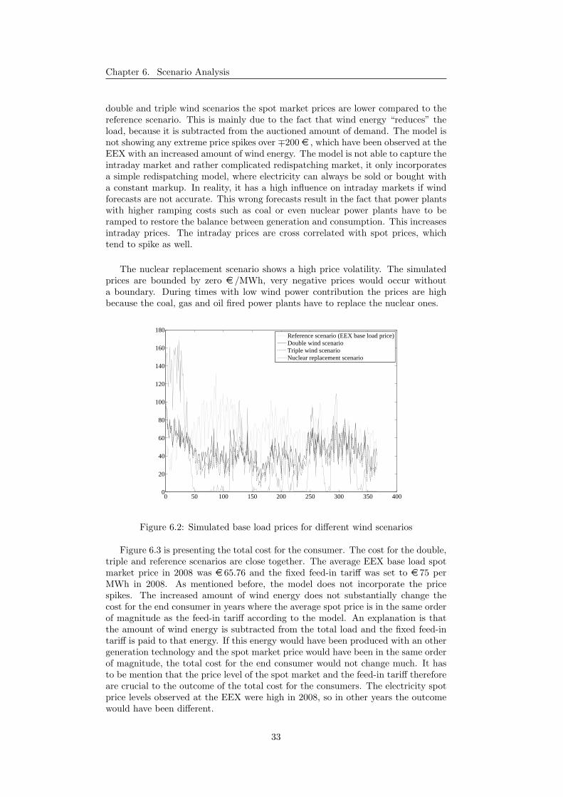
Figure 6.2 shows the spot market prices for the different scenarios. For the

32

Chapter 6. Scenario Analysis

double and triple wind scenarios the spot market prices are lower compared to thereference scenario. This is mainly due to the fact that wind energy “reduces” theload, because it is subtracted from the auctioned amount of demand. The model isnot showing any extreme price spikes over ∓200 e , which have been observed at theEEX with an increased amount of wind energy. The model is not able to capture theintraday market and rather complicated redispatching market, it only incorporatesa simple redispatching model, where electricity can always be sold or bought witha constant markup. In reality, it has a high influence on intraday markets if windforecasts are not accurate. This wrong forecasts result in the fact that power plantswith higher ramping costs such as coal or even nuclear power plants have to beramped to restore the balance between generation and consumption. This increasesintraday prices. The intraday prices are cross correlated with spot prices, whichtend to spike as well.

The nuclear replacement scenario shows a high price volatility. The simulatedprices are bounded by zero e /MWh, very negative prices would occur withouta boundary. During times with low wind power contribution the prices are highbecause the coal, gas and oil fired power plants have to replace the nuclear ones.

0 50 100 150 200 250 300 350 4000

20

40

60

80

100

120

140

160

180

Day

Spo

tpri

ce [

Eur

o/M

Wh]

Reference scenario (EEX base load price)Double wind scenarioTriple wind scenarioNuclear replacement scenario

Figure 6.2: Simulated base load prices for different wind scenarios

Figure 6.3 is presenting the total cost for the consumer. The cost for the double,triple and reference scenarios are close together. The average EEX base load spotmarket price in 2008 was e 65.76 and the fixed feed-in tariff was set to e 75 perMWh in 2008. As mentioned before, the model does not incorporate the pricespikes. The increased amount of wind energy does not substantially change thecost for the end consumer in years where the average spot price is in the same orderof magnitude as the feed-in tariff according to the model. An explanation is thatthe amount of wind energy is subtracted from the total load and the fixed feed-intariff is paid to that energy. If this energy would have been produced with an othergeneration technology and the spot market price would have been in the same orderof magnitude, the total cost for the end consumer would not change much. It hasto be mention that the price level of the spot market and the feed-in tariff thereforeare crucial to the outcome of the total cost for the consumers. The electricity spotprice levels observed at the EEX were high in 2008, so in other years the outcomewould have been different.

33


Another remark is that The agents are not able to substantially increase theirmarket power nor is it a major drawback for their bidding strategies if the stochasticuncertainty of electricity generation is increased.

The electricity cost for the end consumer is higher in the nuclear replacementscenario, especially during times with low wind energy contribution. An importantremark is that in the nuclear replacement scenario the total electricity generation ishigher than the consumption at certain point in time. The wind power can changequite dramatically between two subsequent hours and the power plants are notcapable of ramping their production fast enough. To cover this spread, more gasfired power plants have to be put online or a storage device could be introduced,which brings us to the next section.

0 50 100 150 200 250 300 350 4000.2

0.4

0.6

0.8

1

1.2

1.4

1.6

1.8

2

2.2x 10

8

Day

Tot

al c

ost [

Eur

o]

Reference scenarioDouble wind scenarioTriple wind scenarioNuclear replacement scenario

Figure 6.3: Total electricity cost for the end consumer for different wind scenarios

6.2 Scenarios with a Storage Device

Vehicles that can run on both electricity and gasoline, so called plug-in electricvehicles (PHEVs) are proposed as near term technology to achieve energy andenvironmental goals and as a transitional step toward electric vehicles addressingmany of the same goals. The PHEVs include an internal combustion engine as aprimary and an electric motor as a secondary energy source. Whether PHEVs meetany of their goals depends not only on their design and performance on standardizeddrive cycles, but also on recharging behavior [28]. The PHEVs offer the possibility tosubstantially shift the energy demand for transportation from crude oil to electricity.The PHEVs are recharging their batteries via the electric grid. Their internalcombustion engine is only used as an ancillary power source [29].

The charging of the PHEVs via the electric grid offers additional benefits. Theycould provide storage and supply services to the grid, approximately 96% of thetime [30]. Additionally, they could provide a wide range of services for the electricgeneration chain (ancillary services, regulation, back up power and peak shifting)[31].

34


Several cases are modeled in this thesis with respect to PHEVs to analyze theirbehavior on spot prices. In a first modeling approach, it is assumed that the PHEVsare charged by a given charging distribution. In a second approach, the PHEVswould be charged during the night time (off-peak), when the load is generally lower.This would increase the total electricity demand, but at the same time flatten theload curve. In a third approach, PHEVs are considered which offer the possibilityof feeding energy back to the grid. In addition, their charging/discharging wouldinclude a price dependent behavior [32]. The PHEVs would charge their batterieswith electric energy from the grid if the spot prices would be lower than a certainthreshold and discharge their batteries above this threshold. In the last modelingapproach, the third modeling approach would be taken with additional wind powercontribution to assess the ability of the PHEVs to balance the higher uncertaintyin electricity supply.

6.2.1 Charging Plug-ins With a Given Loading Distribution:Scenario one

In [33] a charging distribution for the PHEV charging is proposed. A slightlymodified loading distribution shown in figure 6.4 is used to assess the effect oncharging PHEVs on spot market prices. The charging distribution shows that thePHEVs are charged during 4 pm and 9 am with a peak loading during 11 pm and4 am. Except of the evening peak, the PHEVs are charged during off-peak hours.The hourly charging probabilities sum to one which implies that a PHEV starts tocharge during a particular hour and is fully charged within that hour. In reality,this assumption is not feasible since PHEVs are usually connected and charged tothe low voltage grid and the power flow is limited [34].

0 1 2 3 4 5 6 7 8 9 10 11 12 13 14 15 16 17 18 19 20 21 22 23 24

0

0.02

0.04

0.06

0.08

0.1

Hour

Loa

ding

Pro

babi

lity

Figure 6.4: PHEV charging probability

Further, it is assumed that there are eight million PHEVs. This would cor-respond that roughly every tenth person in Germany would drive around one ona daily basis. The daily distance dday traveled by the PHEVs is lognormaly dis-tributed with a mean of 50 km and a standard deviation of 40 km. Additionally,it is supposed that the average energy rate kavg of the plug-ins corresponds to 0.2

35


kWh/km according to [35]. The electricity demand EPHEV for the hour h by thePHEVs in [kWh] can be computed according to:

EPHEV = 8 · 106 · dday · kavg ·D(h) (6.1)

Where D(h) is the distribution value from figure 6.4 at hour h.

Figure 6.5 shows the simulated and observed base and peak load spot marketprices with the plug-in scenario one after a five year learning interval. It showsthat the simulated and observed prices deviate during the winter month and arecloser together during the summer. The reason for that is in the merit order. Theaggregated spot market supply curve is much steeper for higher output quantities.During the summer month the electricity demand is in general lower. The additionaldemand by the PHEVs as a result has a lower influence on spot market prices.Figure 6.6 shows the cumulative base load price distribution. The simulated curveis higher and steeper. It indicates that spot prices are more widely distributed overthe whole price range and are generally on higher levels.

0 50 100 150 200 250 300 350 40020

40

60

80

100

120

140

160

180

200

Day

Spo

tpri

ce [

Eur

o/M

Wh]

Peakload price PHEV scenario oneBaseload price PHEV scenario oneBaseload price EEXPeakload price EEX

Figure 6.5: Base and peak load prices in 2008 with plug-in scenario one

Table 6.1 provides a simulation summary. One can notice that the simulatedprices for peak and base load are higher. Surprisingly, the simulated base load pricesare higher than the peak load prices. This would imply that the off-peak demandis dramatically increased by the PHEVs, which are mostly charged during off-peakhours as mentioned. Another remarkable result is that the standard deviation ofthe simulated prices is higher than the observed one. A higher demand duringoff-peak hours would flatten the the daily load curve and decrease the hourly pricevolatility as a consequence. Since the charging of the PHEVs according to thegiven distribution 6.6 does not decrease the price volatility, it can be assumed thatthe daily load pattern is not flatten. A reason for this phenomena could be theassumption that PHEVs can be recharged within an hour. During peak chargingtimes this leads to massive power demands by the PHEVs. This power demandwould occur around midnight. As a consequence, the daily load pattern would havean additional demand peak during midnight beside the one at noon and the one inthe evening. To overcome this problem, another charging pattern is introduced in

36


0 0.1 0.2 0.3 0.4 0.5 0.6 0.7 0.8 0.9 120

40

60

80

100

120

140

160

180

Pri

ce

Simulated base load prices PHEV scenario oneObserved EEX base load prices

Figure 6.6: Cumulative price distribution of the simulated and observed base loadprices in 2008 with plug-in scenario one

the next subsection.

Simulated [e ] forPHEV scenario

one

Observed EEX[e ]

Mean base load price 105.58 65.78

Mean peak load price 102.11 79.44

Std. deviation base load 24.87 18.14

Std. deviation peak load 30.96 24.27

Table 6.1: Simulation summary plug-in scenario one

6.2.2 Charging Plug-ins During Off-Peak Hours: Scenariotwo

In this subsection an alternative charging pattern by the PHEVs is analyzed. [31]suggest that the PHEVs could be charged during the nightly hours to shave it towarda more flatten hourly demand curve. Again, eight million PHEVs are assumed andthe daily driving distance is again lognormally distributed. The main difference tothe plug-in scenario one is that the all the PHEVs are charged after 9 pm. By doingthat, the charging does not amplify the evening demand peak. Additionally, themaximum charging capacity per vehicle is set to 1400 W.

Figure 6.7 and 6.8 show the spot market prices and cumulative base load pricesfor the plug-in scenario two. The price level differences between the observed EEXprices and the simulated prices are again higher during the winter month. Comparedto the plug-in scenario one the general price level is remarkable lower. This isinteresting since the total amount of energy demanded stays the same; the timingof the charing has a major impact on spot market prices.

By analyzing figure 6.9 it is remarkable that all the utilities achieve higher profitscompared to the reference conditions (see figure 5.8). The higher profits are a resultof a generally higher demand on one hand and a more flatten daily load pattern on

37


0 50 100 150 200 250 300 350 40020

40

60

80

100

120

140

160

180

200

Day

Spo

tpri

ce [

Eur

o/M

Wh]

Peakload price PHEV scenario twoBaseload price PHEV scenario twoBaseload price EEXPeakload price EEX

Figure 6.7: Base and peak load prices in 2008 with plug-in scenario two

the other hand. The flatten demand allows the utilities to run the lignite and hardcoal power plants at higher output levels. The gas turbines have to be turned onless and in general the ramping costs are decreased substantially. It can be assumedthat utilities have an incentive to promote PHEVs since they allow to use the powerplants more efficiently and generate higher profits.

38


0 0.1 0.2 0.3 0.4 0.5 0.6 0.7 0.8 0.9 120

40

60

80

100

120

140

160

180P

rice

Simulated base load prices PHEV scenario twoObserved EEX base load prices

Figure 6.8: Cumulative price distribution of the simulated and observed base loadprices in 2008 with plug-in scenario two

0 50 100 150 200 250 300 350 400-1

0

1

2

3

4

5

6x 10

7

Day

Agg

rega

ted

rew

ard

[Eur

o]

E.OnEnBWVattenfallRWEOthers

Figure 6.9: Profit of the different utilities with plug-in scenario two

39


6.2.3 Introducing Plug-ins with Spot Market Price SensitiveCharging Characteristic: Scenario three

In this scenario, a price depending charging is modeled. Additionally, the PHEVsare able to feed energy back to the electric grid during periods with high price levels.Figure 6.10 shows the charging of the PHEVs as a function of the spot market pricet − 1. A similar approach is suggested in [32]. The curve is characterised by fourparameters: The maximum charging power, the maximum discharging power, thethreshold price at which the charing starts to decrease and the switching point wherethe charging is equal to zero. It is assumed that all the PHEVs are connected tothe grid at 5 pm. The maximal charging and discharging rate is set to 1400 W .The threshold price is equal to e 80 and the switching point e 100. A constrain ofthe problem is the PHEVs can not be discharged to a lower level as the level theywere initially connected.

0 20 40 60 80 100 120 140 160 180 200-1500

-1000

-500

0

500

1000

1500

Spot market price [Euro]

Cha

rgin

g [W

]

Figure 6.10: Spot market price depending charging

Figure 6.11 and 6.12 show the spot market prices and cumulative base loadprices for the plug-in scenario three. They both show that the fluctuation in pricelevel in PHEV scenario three is lower compared to scenario one and two. The pricelevel often stays within a certain band. Most prices are in an interval betweene 100 and e 120. The histogram of the simulated base load prices (figure 6.13)confirms this observation. It shows a lot of spot market price observations aroundthe switching point. This has some advantages. The market volatility is a riskmeasure for companies being short on electricity generation. The low volatilitywould decrease the risk and therefore the capital requirements for these firms.

The price levels are rather high in this scenario three. The simulation output ofthe spot market prices is quite crucial to the chosen price threshold and switchingpoint. A problem that occurs is that the PHEVs would buy and sell electricityaround the switching point, pushing market prices above and below the switchingpoint from one hour to the other. This would reduce the life time of the batteries andartificially increase trading volumes. The price would oscillate around the switchingpoint. In stock market this buying and selling mechanism is used to manipulateprices and push stocks to higher price levels. The same effect can be observed here.

40


0 50 100 150 200 250 300 350 40020

40

60

80

100

120

140

160

180

Day

Spo

tpri

ce [

Eur

o/M

Wh]

Peakload price PHEV scenario threeBaseload price PHEV scenario threeBaseload price EEXPeakload price EEX

Figure 6.11: Base and peak load prices in 2008 with plug-in scenario three

The price depending charging by the PHEVs serves as a price cap since athigher prices the discharging energy of the PHEVs is added to the power outputby the power plant. Therefore the prices would not often exceed this price cap.But at the same time there is a strong increase in electricity demand below theswitching point of the PHEVs. The power generating agents experience this strongincrease after a drop in spot market price. As a result, the gas and oil fired powerplants would learn to send inelastic bidding curves to the central market place. Theconsequence is that market prices fall from one hour to the next, but the electricitydemand for the next hour increases by the PHEVs. Since the bidding curves arequite inelastic, prices would jump above the PHEV’s switching point again. Thisprice above the switching point would then imply that the PHEVs are dischargingtheir batteries and adding their energy to the electricity generation, prices would fallagain and so on. The spot price would jump around the switching point. The priceswould be locked in at the switching point, even if excess generation capacity wouldbe available and generation cost would be substantially lower than the switchingpoint. The agents are able to set a price floor by strategic bidding. The agents areable to act strategically since the price depending charging of the PHEVs makesthe load more predictable. A more predictable load pattern in general results in anincreased strategic behavior of the agents and an increase in market power.

41


0 0.1 0.2 0.3 0.4 0.5 0.6 0.7 0.8 0.9 120

40

60

80

100

120

140

160

Pri

ceSimulated base load prices PHEV scenario threeObserved EEX base load prices

Figure 6.12: Cumulative price distribution of the simulated and observed base loadprices in 2008 with plug-in scenario three

40 60 80 100 120 140 1600

10

20

30

40

50

60

Price range [Euro]

Num

ber

of o

bser

vati

ons

Figure 6.13: Histogram of the simulated spot market prices visualizes the locked ineffect

42


6.2.4 Introducing Plug-ins with Spot Market Price SensitiveCharging Characteristic and Increased Wind Contri-bution: Scenario four

The PHEVs are a good complement to the wind energy, which introduces stochasticuncertainty in production. The PHEVs can store excess amount of energy andfeed it back to the electric grid during peak demands. In this fourth scenario,the installed wind capacity is tripled from today’s level to 70.8 MW . The pricethreshold and switching point of the PHEV charging are reduced to e 70 and e 80.

Figure 6.14 show the spot market prices for the plug-in scenario four. Thesimulated spot prices show a low price volatility like the plug-in scenario three,but with a lower price level as the scenario three. This simulation shows that thePHEVs are a good measure to effectively store excess wind power.

0 50 100 150 200 250 300 350 40020

40

60

80

100

120

140

160

180

Day

Spo

tpri

ce [

Eur

o/M

Wh]

Peakload price PHEV scenario fourBaseload price PHEV scenario fourBaseload price EEXPeakload price EEX

Figure 6.14: Base and peak load prices in 2008 with plug-in scenario four

Simulated [e ] forPHEV scenario

four

Observed EEX[e ]

Mean base load price 75.86 65.78

Mean peak load price 77.70 79.44

Std. deviation base load 8.86 18.14

Std. deviation peak load 9.58 24.27

Table 6.2: Simulation summary plug-in scenario four

Again, the output price level is crucial to the chosen price threshold and switch-ing point. It is unclear to what extend the lower price levels in the plug-in scenariofour is a result of the lower switching price by the PHEVs or if the increased installedwind capacity is causing it. In general, the price depending charging is like a closed-loop system that stabilizes prices around the switching point. There is probablya big potential in more advanced charging algorithms that are anticipating certainprice movements and resulting in generally lower price levels. They should be lesspredictable by the power generating agents to decrease their strategic behavior andas a consequence their market power.

43

Chapter 7

Conclusion

Throughout the thesis an agent-based model is used to simulate spot market prices,which are compared to observed EEX prices. The agents in the model are able tolearn and anticipate the input data to increase their own and the reward of thecorresponding utility by using a reinforcement and a genetic algorithm. By biddingin a more strategic way, they are able to increase spot market prices to levels whichare observed at the EEX market.

Agent-based models can provide insights into pricing and strategic behavior inmarkets such as electricity where the single actors act within bounded rationality.Imperfect competition, exercised through the daily repetition of a competitive mar-ket with administrated market rules creates a process of continuous experimentationand gaming that agent-based simulation is able to imitate.

An increase in stochastic uncertainty of power production by doubling or eventripling the installed wind power does not substantially change the cost for theelectricity consumers. The spot market price level decreases but since the windgenerators receive a fixed feed-in tariff the effect on end consumers is minor. Themodel is not able to simulate price spikes, which have been observed at the EEXwith an increased wind energy contribution. These spikes have for instance a biginfluence on the risk management for certain consumers. The spikes increase themarket VAR (value at risk) and therefore the capital requirements. Therefore,additional charges have to be added to the cost of the consumers. The simulationhas been done in a year with a high price level, during years with lower price levelsthe difference in the cost for the consumers most likely increases. Replacing thefixed feed-in tariff with a more market based instrument could help decrease thespot price volatility since it is often cheaper to shut down wind power plants thanramp coal or even nuclear power plants. Replacing nuclear power plants with windenergy changes the price pattern on the spot market as well as the cost for theend consumer dramatically. It increases the spot price volatility and the cost levelfor the consumer, especially during low wind hours. The back up power installedtoday would not be sufficient during such hours to jump in for spreads in electricitygeneration and consumption

The effect of adding plug-in hybrid electric vehicles is investigated with fourdifferent charging scenarios. Charging PHEVs with a given charging distributionor during off-peak hours increases spot price volatility and price levels especiallyduring the winter time, eventhough the PHEVs flattened the hourly electricitydemand. The utilities are able to increase their profits quite substantially with this

44

Chapter 7. Conclusion

additional load. Using a simple price depending charging mechanism and givingthe PHEVs the ability to discharge the batteries during high price levels reducesspot price volatility, even if the installed wind energy power is tripled. But theprice level outcome is very crucial to the chosen switching price between chargingand discharging of the PHEVs. The price depending charging results in a closedloop system that locks in prices at the chosen switching price. Generators learn toanticipate the effect of the increased electricity demand below the switching pointand are able to set a floor at the switching price by restricting power output, evenif marginal cost of production would be much lower. The price dependent chargingshould be replaced by a more advanced algorithm that is able to anticipate pricemovements in order to bring the spot prices to lower levels.

45

List of Figures

1.1 Base load spot price development from the year 2003 to 2009 . . . . 3

2.1 Schematic representation of the LCS learning algorithm . . . . . . . 72.2 Example of the different genetic operations . . . . . . . . . . . . . . 10

3.1 Flow Chart of the Simulator . . . . . . . . . . . . . . . . . . . . . . . 13

4.1 The power plants are receiving an environmental input . . . . . . . . 194.2 Bidding of the nuclear, hard coal and lignite power stations . . . . . 204.3 Bidding of the oil and gas fired power stations . . . . . . . . . . . . . 214.4 Market clearing with redispatching . . . . . . . . . . . . . . . . . . . 224.5 Profit calculation of the agents . . . . . . . . . . . . . . . . . . . . . 23

5.1 Simulated and observed EEX base and peak load prices in 2008 underreference condition . . . . . . . . . . . . . . . . . . . . . . . . . . . . 25

5.2 Cumulative price distribution of the simulated and observed baseload prices in 2008 under reference condition . . . . . . . . . . . . . 26

5.3 Simulated and observed EEX base and peak load prices in 2008,simulation setting optimized with information sharing . . . . . . . . 27

5.4 Cumulative price distribution of the simulated and observed base loadprices in 2008 after the learning process, simulation setting optimizedwith information sharing . . . . . . . . . . . . . . . . . . . . . . . . 28

5.5 Cumulative price distribution of the simulated and observed base loadprices in 2008 after the learning process, simulation setting optimizedwithout information sharing . . . . . . . . . . . . . . . . . . . . . . 29

5.6 Hourly traded electricity volume over the EEX spot market . . . . . 305.7 Daily electricity output levels of the different generation technologies 305.8 Profit of the different utilities . . . . . . . . . . . . . . . . . . . . . . 31

6.1 Day ahead wind forecast error . . . . . . . . . . . . . . . . . . . . . . 326.2 Simulated base load prices for different wind scenarios . . . . . . . . 336.3 Total electricity cost for the end consumer for different wind scenarios 346.4 PHEV charging probability . . . . . . . . . . . . . . . . . . . . . . . 356.5 Base and peak load prices in 2008 with plug-in scenario one . . . . . 366.6 Cumulative price distribution of the simulated and observed base

load prices in 2008 with plug-in scenario one . . . . . . . . . . . . . . 376.7 Base and peak load prices in 2008 with plug-in scenario two . . . . . 386.8 Cumulative price distribution of the simulated and observed base

load prices in 2008 with plug-in scenario two . . . . . . . . . . . . . 396.9 Profit of the different utilities with plug-in scenario two . . . . . . . 396.10 Spot market price depending charging . . . . . . . . . . . . . . . . . 406.11 Base and peak load prices in 2008 with plug-in scenario three . . . . 41

46

List of Figures

6.12 Cumulative price distribution of the simulated and observed baseload prices in 2008 with plug-in scenario three . . . . . . . . . . . . . 42

6.13 Histogram of the simulated spot market prices visualizes the lockedin effect . . . . . . . . . . . . . . . . . . . . . . . . . . . . . . . . . . 42

6.14 Base and peak load prices in 2008 with plug-in scenario four . . . . . 43

47

List of Tables

3.1 Generator specific parameters of the cost model . . . . . . . . . . . . 15

4.1 Utilities and their maximal output power per generation technology,source EEX . . . . . . . . . . . . . . . . . . . . . . . . . . . . . . . . 17

5.1 Simulation summary reference conditions . . . . . . . . . . . . . . . 29

6.1 Simulation summary plug-in scenario one . . . . . . . . . . . . . . . 376.2 Simulation summary plug-in scenario four . . . . . . . . . . . . . . . 43

48

Bibliography

[1] L. Ruff, “Stop wheeling and start dealing: Resolving the transmissiondilemma,” in Electricity Transmission Pricing and Technology, M. Einhornand E. S. Riaz, Eds. Boston: Kluwer Academics Publisher Group, 1996.

[2] D. J. Veit, A. Weidlich, and J. A. Krafft, “An agent-based analysis of the ger-man electricity market with transmission capacity constraints,” Energy Policy,vol. 37, pp. 4132–4144, 2009.

[3] J. Bower, D. W. Bunn, and C. Wattendrup, “A model-based analysis of strate-gic consolidation in the german electricity industry,” Energy Policy 29, pp.987–1005, 2001.

[4] F. Musgens, “Quantifying market power in the german wholesale electricitymarket using a dynamic multi-regional dispatch model,” The Journal of In-dustrial Economics, vol. LIV, pp. 471–498, December 2006.

[5] C. Growitsch and R. Nepal, “Efficiency of the german electricity wholesale mar-ket,” European transactions on electrical power, vol. 19, pp. 553–568, February2009.

[6] Council of European Energy Regulators ASBL, “The green package - proposedeu ets and renewables directives,” Ref: C08-SDE-02-06, pp. 2–11, May 2008.

[7] “Commission plans legislative framework to ensure the eu meets its target forcutting co2 emissions from cars,” IP/07/155, February 2007.

[8] B. D. Williams and K. S. Kurani, “Commercializing light-duty plug-in/plug-outhydrogen-fuel-cell vehicles: mobile electricity technologies and opportunities,”Journal of Power Sources, vol. 166, no. 2, pp. 549–566, 2007.

[9] M. D. Galus and G. Andersson, “Integration of plug-in hybrid electric vehiclesinto energy networks,” in 2009 IEEE Bucharest PowerTech (POWERTECH),2009, p. 8 pp.

[10] R. L. Axtell, C. J. Andrews, and M. J. Small. (2003, October)Agent-based models of industrial ecosystems. [Online]. Available: http://policy.rutgers.edu/andrews/projects/abm/abmarticle.htm

[11] E. Bonabeau, “Agent-based modeling: Methods and techniques for simulatinghuman systems,” in National Academy of Science, May 2002.

[12] M. Wooldridge and N. Jennings, “Intelligent agents: Theory and practice,”Knowledge Engineering Review, vol. 10, no. 2, 1995.

[13] J. H. Holland, L. B. Booker, M. Colombetti, M. Dorigo, D. E. Goldberg, S. For-rest, R. L. Riolo, R. E. Smith, P. L. Lanzi, W. Stolzmann, and S. W. Wilson,What Is a Learning Classifier System? Springer Berlin / Heidelberg, 2000.

49

http://policy.rutgers.edu/andrews/projects/abm/abmarticle.htm

http://policy.rutgers.edu/andrews/projects/abm/abmarticle.htm

Bibliography

[14] A. Bernauer, “Das learning classifier system xcs,” pp. 1–12, 7 2007.

[15] T. Krause and G. Andersson, “Evaluating congestion management schemes inliberalized electricity markets using an agent-based simulator,” IEEE PowerEngineering Society General Meeting, pp. 377–384, 2006.

[16] S. W. Wilson, “Classifier fitness based on accuracy,” Evolutionary Computa-tion, vol. 3, no. 2, pp. 149–175, 1995.

[17] M. V. Butz and S. W. Wilson, “An algorithmic description of xcs,” Soft Com-puting, vol. 6, pp. 144–153, 2002.

[18] M. V. Butz, “Rule-based evolutionary online learning systems,” Studies inFuzziness and Soft Computing, vol. 191, pp. 51–64, 2006.

[19] A. Orriols-Puig, D. E. Goldberg, K. Sastry, and E. Bernado-Mansilla, “Model-ing xcs in class imbalances: Population size and parameter settings,” Geneticand evolutionary computation conference, vol. 1 and 2, pp. 1838–1845, 2007.

[20] B. Hobbs, C. Metzler, and J.-S. Pang, “Strategic gaming analysis for electricpower systems: an mpec approach,” Power Systems, IEEE Transactions on,vol. 15, no. 2, pp. 638–645, 2000.

[21] D. W. Bunn and F. S. Oliveira, “Agent-based simulation - an application to thenew electricity trading arrangements of england and wales,” IEEE transactionson evolutionary computation, vol. 5, no. 5, pp. 493–503, October 2001.

[22] D. M. Newbery, “Power markets and market power,” Energy J, vol. 16, pp.39–66, 1995.

[23] A. Tversky and D. Kahneman, “Belief in the law of small numbers,” Pscholog-ical bulletin, vol. 76, no. 2, pp. 105–110, 1971.

[24] F. Musgen, “Market power in the german wholesale electricity market,” EWIWorking Paper, no. 04.03, pp. 1–29, 2004.

[25] (2008, July) Eex produktbroschure strom. [Online]. Available: http://www.eex.com/en/Download/Documentation

[26] (2007, January) Einfuhrung in den borsenhandel an der eex auf xetra.[Online]. Available: http://www.eex.com/en/Download/Documentation

[27] P. L. Lanzi, “Using raw accuracy to estimate classifier fitness in xcs,” Geneticand evolutionary computation - GECCO, vol. 2724, pp. 1922–1923, 2003.

[28] J. Axsen and K. Kurani, “The early u.s. market for phevs: Anticipating con-sumer awarness, recharge potential, design priorities and energy impacts,”Publication of the Institute of Transportation Studies, University of Califor-nia Davis, CA, vol. UCD-ITS-RR-08-22, 2008.

[29] J. Tomic and W. Kempton, “Using fleets of electric-driven vehicles for gridsupport,” Journal of Power Sources, vol. 168, no. 2, pp. 459–469, 2007.

[30] W. Kempton and S. Letendre, “Electric vehicles as a new power source forelectric utilities,” Trans. Res., vol. 2, 1997.

[31] P. Kadured, C. Iokimidis, and P. Ferrao, “Electric vehicles and their impact tothe electric grid in isolated systems,” Powereng, pp. 49–54, March 2009.

50

http://www.eex.com/en/Download/Documentation



Bibliography

[32] M. Galus and G. Andersson, “Demand management of grid connected plug-inhybrid electric vehicles (phev),” 2008 IEEE Energy 2030 Conference, p. 8 pp.,2008.

[33] C. Roe, Dr. A.P. Meliopoulos, F. Evangelos, and Dr. T. Overbye, “Powersystem level impacts of phevs,” in 42nd Hawaii International Conference onSystem Sciences, 2009.

[34] R. A. Waraich, M. Galus, C. Dobler, M. Balmer, G. Andersson, and K. W. Ax-hausen, “Plug-in hybrid electric vehicles and smart grid: Investigations basedon a micro-simulation,” The 12th International Conference of the InternationalAssociation for Travel Behaviour Research, Jaipur, India, 2009.

[35] A. Shortt and M. O’Malley, “Impact of optimal charging of electric vehicleson future generation portfolios,” in In review for IEEE PES/IAS sustainablealternative energy conference, Valencia, Spain, 2009.

51

Agent-Based Simulator for the German Electricity Wholesale ... · Agent-Based Simulator for the...

Documents

Transcript of Agent-Based Simulator for the German Electricity Wholesale ... · Agent-Based Simulator for the...