Agenda - Department of Computer Science and … We've done Greedy Method Divide and Conquer Dynamic...
27
Agenda We’ve done Greedy Method Divide and Conquer Dynamic Programming Network Flows & Applications NP-completeness Now Linear Programming and the Simplex Method Hung Q. Ngo (SUNY at Buffalo) CSE 531 1 / 59 Linear Programming Motivation: The Diet Problem Setting n foods (beef, apple, potato chips, pho, b´ un b` o, etc.) m nutritional elements (vitamins, calories, etc.) each gram of j th food contains a ij units of nutritional element i a good meal needs b i units of nutritional element i each gram of j th food costs c j Objective design the most economical meal yet dietarily sufficient (Halliburton must solve this problem!) Hung Q. Ngo (SUNY at Buffalo) CSE 531 3 / 59
Transcript of Agenda - Department of Computer Science and … We've done Greedy Method Divide and Conquer Dynamic...
Agenda
We’ve done
Greedy Method
Divide and Conquer
Dynamic Programming
Network Flows & Applications
NP-completeness
Now
Linear Programming and the Simplex Method
Hung Q. Ngo (SUNY at Buffalo) CSE 531 1 / 59
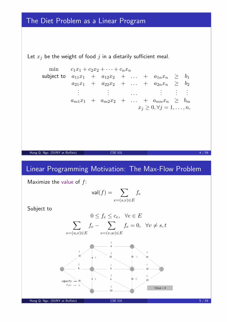
Linear Programming Motivation: The Diet Problem
Setting
n foods (beef, apple, potato chips, pho, bun bo, etc.)
m nutritional elements (vitamins, calories, etc.)
each gram of jth food contains aij units of nutritional element i
a good meal needs bi units of nutritional element i
each gram of jth food costs cj
Objective
design the most economical meal yet dietarily sufficient
(Halliburton must solve this problem!)
Hung Q. Ngo (SUNY at Buffalo) CSE 531 3 / 59
The Diet Problem as a Linear Program
Let xj be the weight of food j in a dietarily sufficient meal.
min c1x1 + c2x2 + · · ·+ cnxn
subject to a11x1 + a12x2 + . . . + a1nxn ≥ b1
a21x1 + a22x2 + . . . + a2nxn ≥ b2...
... . . ....
......
am1x1 + am2x2 + . . . + amnxn ≥ bm
xj ≥ 0,∀j = 1, . . . , n,
Hung Q. Ngo (SUNY at Buffalo) CSE 531 4 / 59
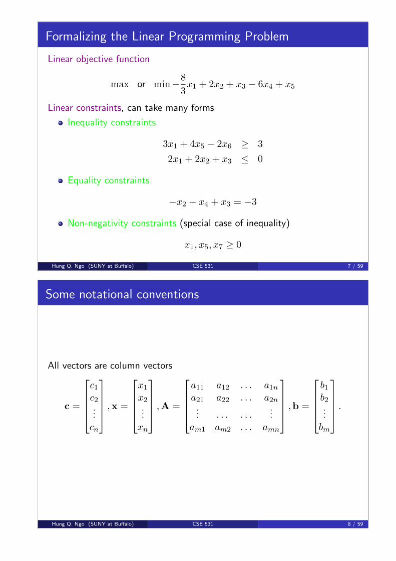
Linear Programming Motivation: The Max-Flow Problem
Maximize the value of f :
val(f) =∑
e=(s,v)∈E
fe
Subject to0 ≤ fe ≤ ce, ∀e ∈ E∑
e=(u,v)∈E
fe −∑
e=(v,w)∈E
fe = 0, ∀v 6= s, t
Hung Q. Ngo (SUNY at Buffalo) CSE 531 5 / 59
Formalizing the Linear Programming Problem
Linear objective function
max or min−83x1 + 2x2 + x3 − 6x4 + x5
Linear constraints, can take many forms
Inequality constraints
3x1 + 4x5 − 2x6 ≥ 32x1 + 2x2 + x3 ≤ 0
Equality constraints
−x2 − x4 + x3 = −3
Non-negativity constraints (special case of inequality)
x1, x5, x7 ≥ 0
Hung Q. Ngo (SUNY at Buffalo) CSE 531 7 / 59
Some notational conventions
All vectors are column vectors
c =
c1
c2...
cn
,x =
x1
x2...
xn
,A =
a11 a12 . . . a1n
a21 a22 . . . a2n... . . . . . .
...am1 am2 . . . amn
,b =
b1
b2...
bm
.
Hung Q. Ngo (SUNY at Buffalo) CSE 531 8 / 59
Linear Program: Standard Form
min / max c1x1 + c2x2 + · · ·+ cnxn
subject to a11x1 + a12x2 + . . . + a1nxn = b1
a21x1 + a22x2 + . . . + a2nxn = b2...
... . . .... =
...am1x1 + am2x2 + . . . + amnxn = bm
xj ≥ 0,∀j = 1, . . . , n,
or, in matrix notations,
min / max{cTx | Ax = b,x ≥ 0
}
Hung Q. Ngo (SUNY at Buffalo) CSE 531 9 / 59
Linear Program: Canonical Form – min Version
min c1x1 + c2x2 + · · ·+ cnxn
subject to a11x1 + a12x2 + . . . + a1nxn ≥ b1
a21x1 + a22x2 + . . . + a2nxn ≥ b2...
... . . .... ≥
...am1x1 + am2x2 + . . . + amnxn ≥ bm
xj ≥ 0,∀j = 1, . . . , n,
or, in matrix notations,
min{cTx | Ax ≥ b,x ≥ 0
}
Hung Q. Ngo (SUNY at Buffalo) CSE 531 10 / 59
Linear Program: Canonical Form – max Version
max c1x1 + c2x2 + · · ·+ cnxn
subject to a11x1 + a12x2 + . . . + a1nxn ≤ b1
a21x1 + a22x2 + . . . + a2nxn ≤ b2...
... . . .... ≤
...am1x1 + am2x2 + . . . + amnxn ≤ bm
xj ≥ 0,∀j = 1, . . . , n,
or, in matrix notations,
max{cTx | Ax ≤ b,x ≥ 0
}
Hung Q. Ngo (SUNY at Buffalo) CSE 531 11 / 59
Conversions Between Forms of Linear Programs
max cTx = min(−c)Tx∑j aijxj = bi is equivalent to
∑j aijxj ≤ bi and
∑j aijxj ≥ bi.∑
j aijxj ≤ bi is equivalent to −∑
j aijxj ≥ −bi∑j aijxj ≤ bi is equivalent to
∑j aijxj + si = bi, si ≥ 0. The
variable si is called a slack variable.
When xj ≤ 0, replace all occurrences of xj by −x′j , and replacexj ≤ 0 by x′j ≥ 0.
When xj is not restricted in sign, replace it by (uj − vj), anduj , vj ≥ 0.
Hung Q. Ngo (SUNY at Buffalo) CSE 531 12 / 59

Example of Converting Linear Programs
Writemin x1 − x2 + 4x3
subject to 3x1 − x2 = 3− x2 + 2x4 ≥ 4
x1 + x3 ≤ −3x1, x2 ≥ 0
in standard (min / max) form and canonical (min / max) form.
Hung Q. Ngo (SUNY at Buffalo) CSE 531 13 / 59
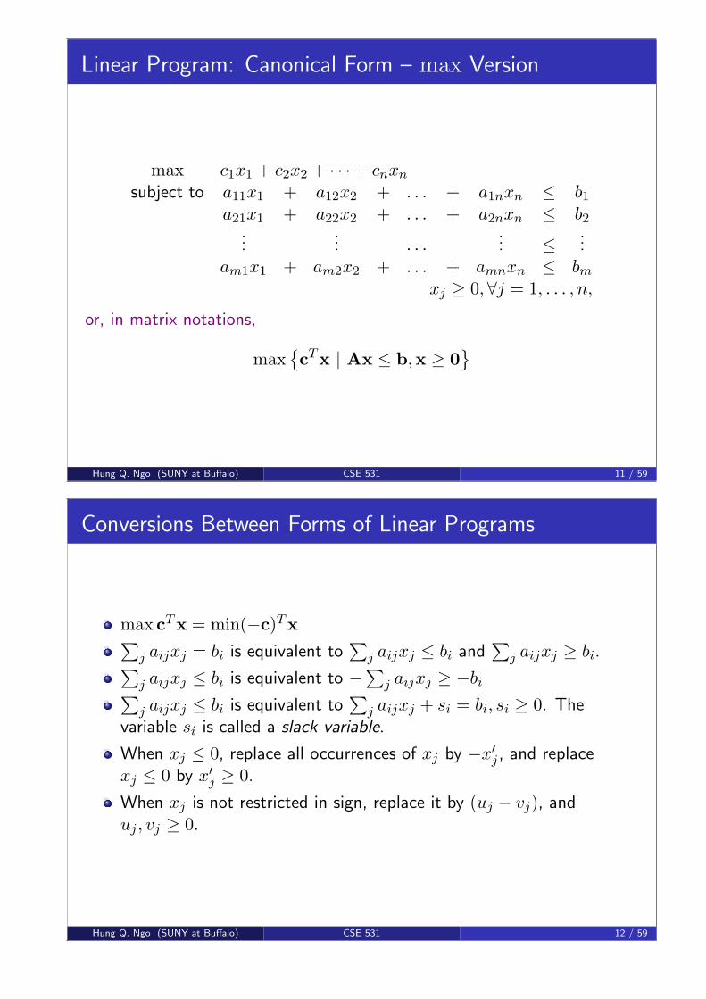
LP Geometry: Example 1
max 2x + ysubject to −2x + y ≤ 2
5x + 3y ≤ 15x + y ≤ 4
x ≥ 0, y ≥ 0
Hung Q. Ngo (SUNY at Buffalo) CSE 531 15 / 59
Example 1 – Feasible Region
Hung Q. Ngo (SUNY at Buffalo) CSE 531 16 / 59
Example 1 – Objective Function
Hung Q. Ngo (SUNY at Buffalo) CSE 531 17 / 59
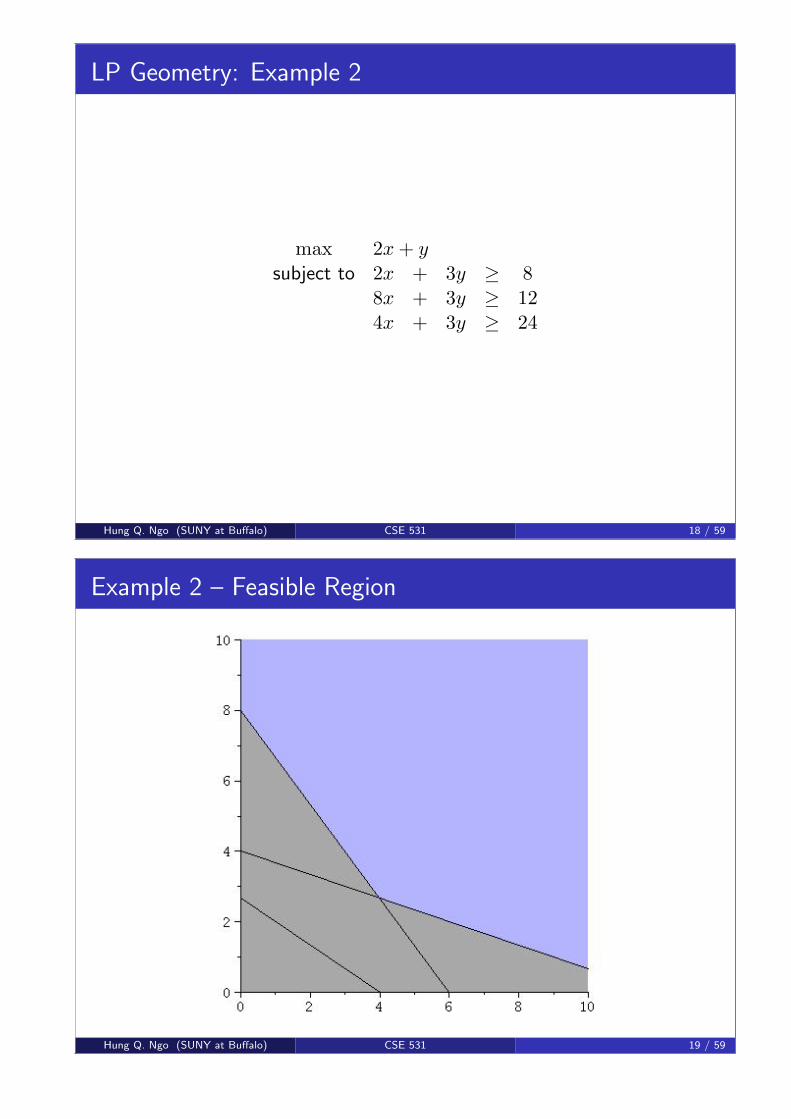
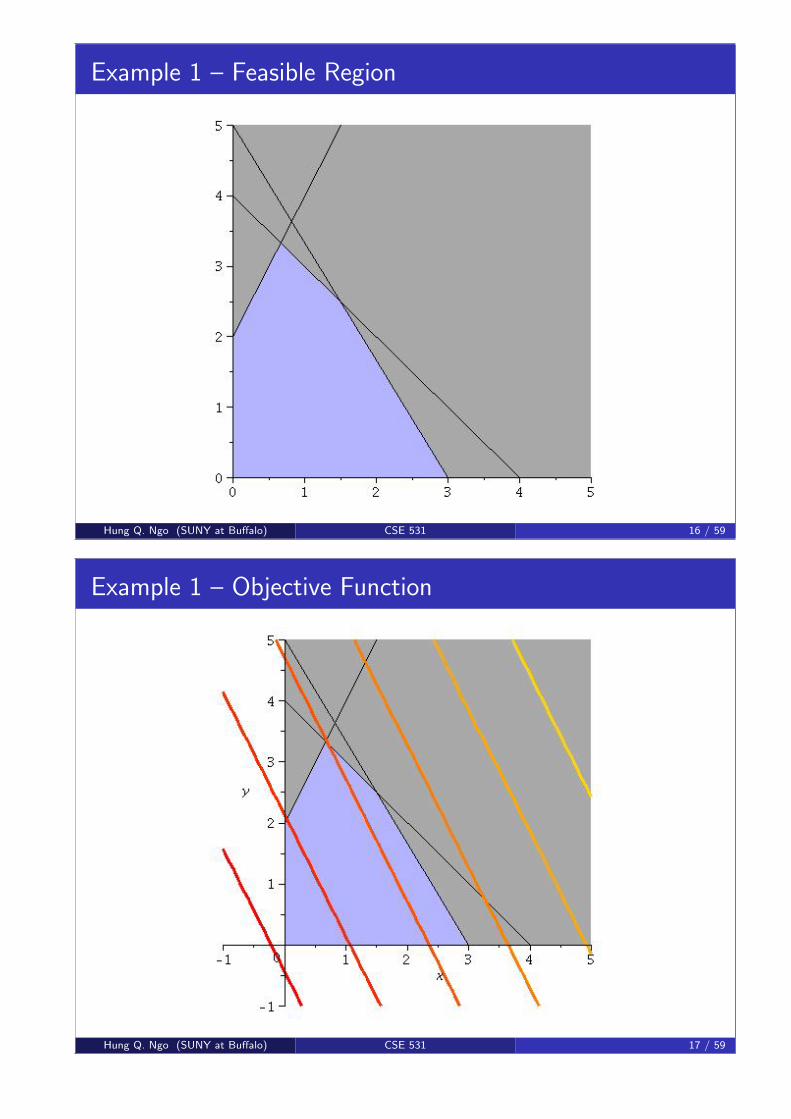
LP Geometry: Example 2
max 2x + ysubject to 2x + 3y ≥ 8
8x + 3y ≥ 124x + 3y ≥ 24
Hung Q. Ngo (SUNY at Buffalo) CSE 531 18 / 59
Example 2 – Feasible Region
Hung Q. Ngo (SUNY at Buffalo) CSE 531 19 / 59
Example 2 – Objective Function
Hung Q. Ngo (SUNY at Buffalo) CSE 531 20 / 59
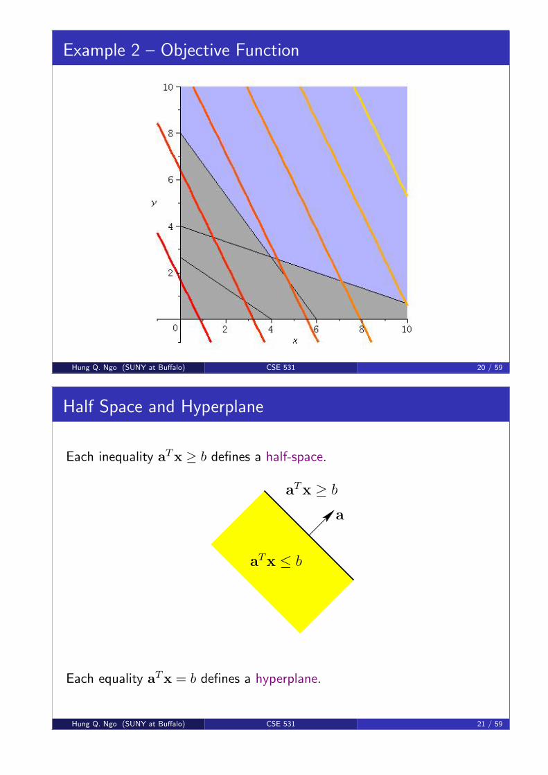
Half Space and Hyperplane
Each inequality aTx ≥ b defines a half-space.
a
aTx ≥ b
aTx ≤ b
Each equality aTx = b defines a hyperplane.
Hung Q. Ngo (SUNY at Buffalo) CSE 531 21 / 59
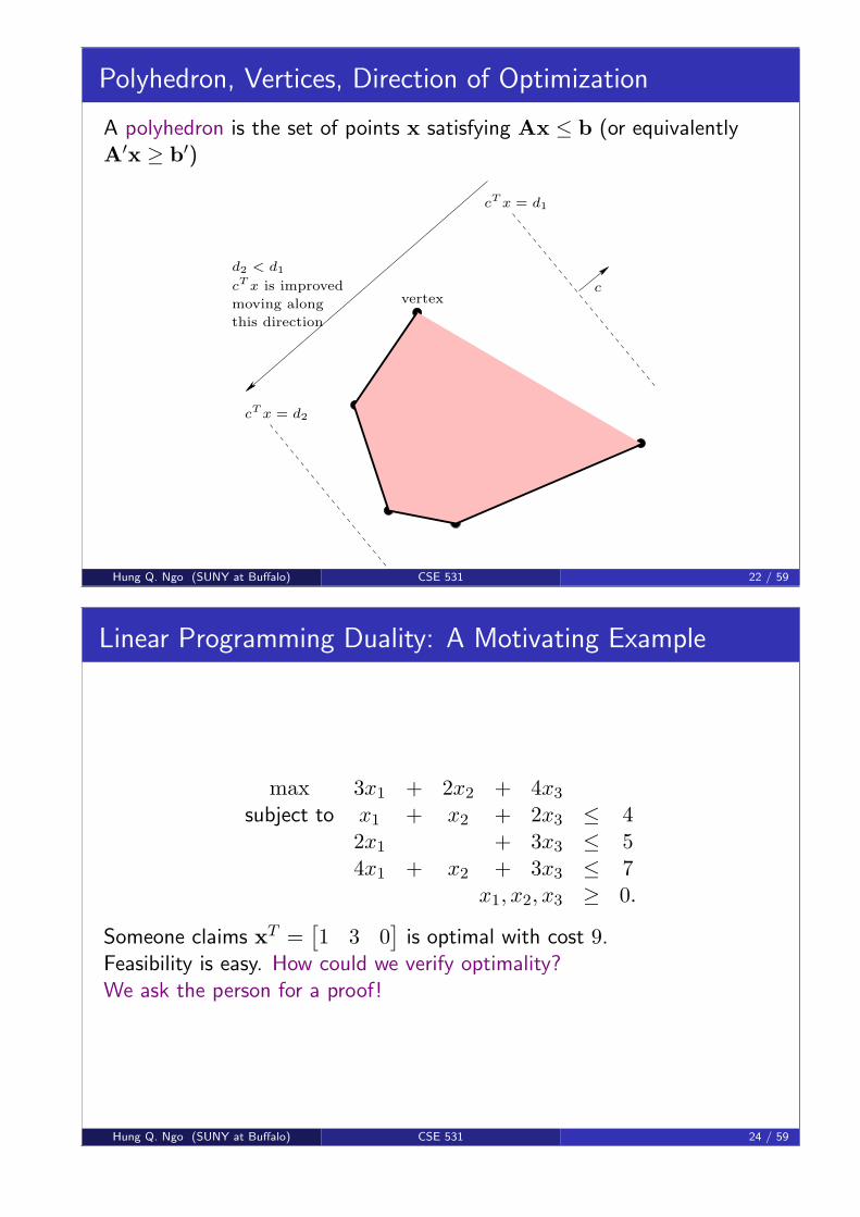
Polyhedron, Vertices, Direction of Optimization
A polyhedron is the set of points x satisfying Ax ≤ b (or equivalentlyA′x ≥ b′)
cT x = d2
vertex
cT x = d1
moving along
this direction
cT x is improved
d2 < d1
c
Hung Q. Ngo (SUNY at Buffalo) CSE 531 22 / 59
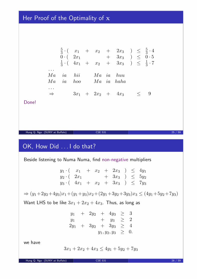
Linear Programming Duality: A Motivating Example
max 3x1 + 2x2 + 4x3
subject to x1 + x2 + 2x3 ≤ 42x1 + 3x3 ≤ 54x1 + x2 + 3x3 ≤ 7
x1, x2, x3 ≥ 0.
Someone claims xT =[1 3 0
]is optimal with cost 9.
Feasibility is easy. How could we verify optimality?We ask the person for a proof!
Hung Q. Ngo (SUNY at Buffalo) CSE 531 24 / 59
Her Proof of the Optimality of x
53 · ( x1 + x2 + 2x3 ) ≤ 5
3 · 40 · ( 2x1 + 3x3 ) ≤ 0 · 513 · ( 4x1 + x2 + 3x3 ) ≤ 1
3 · 7. . .Ma ia hii Ma ia huuMa ia hoo Ma ia haha. . .⇒ 3x1 + 2x2 + 4x3 ≤ 9
Done!
Hung Q. Ngo (SUNY at Buffalo) CSE 531 25 / 59
OK, How Did . . . I do that?
Beside listening to Numa Numa, find non-negative multipliers
y1 · ( x1 + x2 + 2x3 ) ≤ 4y1
y2 · ( 2x1 + 3x3 ) ≤ 5y2
y3 · ( 4x1 + x2 + 3x3 ) ≤ 7y3
⇒ (y1+2y2+4y3)x1+(y1+y3)x2+(2y1+3y2+3y3)x3 ≤ (4y1+5y2+7y3)
Want LHS to be like 3x1 + 2x2 + 4x3. Thus, as long as
y1 + 2y2 + 4y3 ≥ 3y1 + y3 ≥ 22y1 + 3y2 + 3y3 ≥ 4
y1, y2, y3 ≥ 0.
we have3x1 + 2x2 + 4x3 ≤ 4y1 + 5y2 + 7y3
Hung Q. Ngo (SUNY at Buffalo) CSE 531 26 / 59
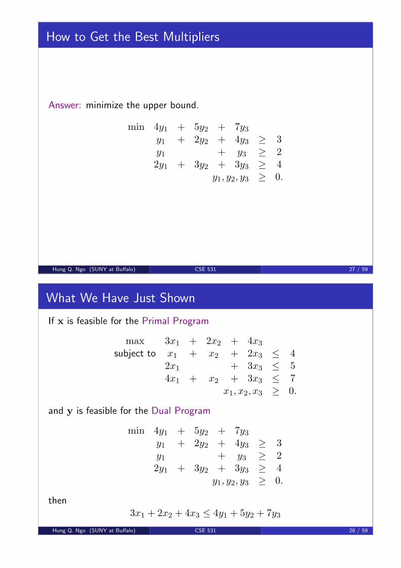
How to Get the Best Multipliers
Answer: minimize the upper bound.
min 4y1 + 5y2 + 7y3
y1 + 2y2 + 4y3 ≥ 3y1 + y3 ≥ 22y1 + 3y2 + 3y3 ≥ 4
y1, y2, y3 ≥ 0.
Hung Q. Ngo (SUNY at Buffalo) CSE 531 27 / 59
What We Have Just Shown
If x is feasible for the Primal Program
max 3x1 + 2x2 + 4x3
subject to x1 + x2 + 2x3 ≤ 42x1 + 3x3 ≤ 54x1 + x2 + 3x3 ≤ 7
x1, x2, x3 ≥ 0.
and y is feasible for the Dual Program
min 4y1 + 5y2 + 7y3
y1 + 2y2 + 4y3 ≥ 3y1 + y3 ≥ 22y1 + 3y2 + 3y3 ≥ 4
y1, y2, y3 ≥ 0.
then3x1 + 2x2 + 4x3 ≤ 4y1 + 5y2 + 7y3
Hung Q. Ngo (SUNY at Buffalo) CSE 531 28 / 59
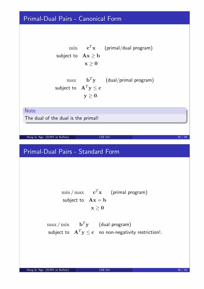
Primal-Dual Pairs - Canonical Form
min cTx (primal/dual program)
subject to Ax ≥ b
x ≥ 0
max bTy (dual/primal program)
subject to ATy ≤ c
y ≥ 0.
Note
The dual of the dual is the primal!
Hung Q. Ngo (SUNY at Buffalo) CSE 531 29 / 59
Primal-Dual Pairs - Standard Form
min / max cTx (primal program)
subject to Ax = b
x ≥ 0
max / min bTy (dual program)
subject to ATy ≤ c no non-negativity restriction!.
Hung Q. Ngo (SUNY at Buffalo) CSE 531 30 / 59
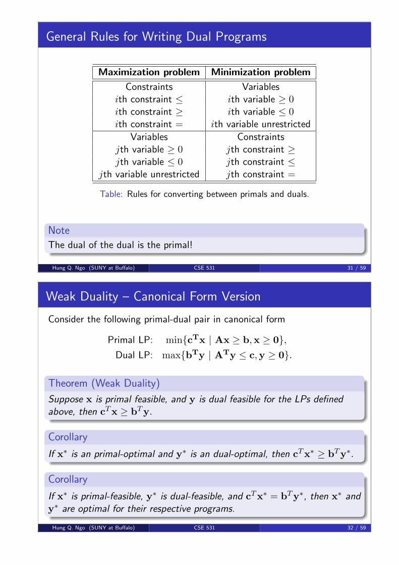
General Rules for Writing Dual Programs
Maximization problem Minimization problem
Constraints Variablesith constraint ≤ ith variable ≥ 0ith constraint ≥ ith variable ≤ 0ith constraint = ith variable unrestricted
Variables Constraintsjth variable ≥ 0 jth constraint ≥jth variable ≤ 0 jth constraint ≤
jth variable unrestricted jth constraint =
Table: Rules for converting between primals and duals.
Note
The dual of the dual is the primal!
Hung Q. Ngo (SUNY at Buffalo) CSE 531 31 / 59
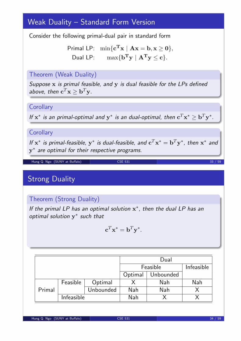
Weak Duality – Canonical Form Version
Consider the following primal-dual pair in canonical form
Primal LP: min{cTx | Ax ≥ b,x ≥ 0},Dual LP: max{bTy | ATy ≤ c,y ≥ 0}.
Theorem (Weak Duality)
Suppose x is primal feasible, and y is dual feasible for the LPs definedabove, then cTx ≥ bTy.
Corollary
If x∗ is an primal-optimal and y∗ is an dual-optimal, then cTx∗ ≥ bTy∗.
Corollary
If x∗ is primal-feasible, y∗ is dual-feasible, and cTx∗ = bTy∗, then x∗ andy∗ are optimal for their respective programs.
Hung Q. Ngo (SUNY at Buffalo) CSE 531 32 / 59
Weak Duality – Standard Form Version
Consider the following primal-dual pair in standard form
Primal LP: min{cTx | Ax = b,x ≥ 0},Dual LP: max{bTy | ATy ≤ c}.
Theorem (Weak Duality)
Suppose x is primal feasible, and y is dual feasible for the LPs definedabove, then cTx ≥ bTy.
Corollary
If x∗ is an primal-optimal and y∗ is an dual-optimal, then cTx∗ ≥ bTy∗.
Corollary
If x∗ is primal-feasible, y∗ is dual-feasible, and cTx∗ = bTy∗, then x∗ andy∗ are optimal for their respective programs.
Hung Q. Ngo (SUNY at Buffalo) CSE 531 33 / 59
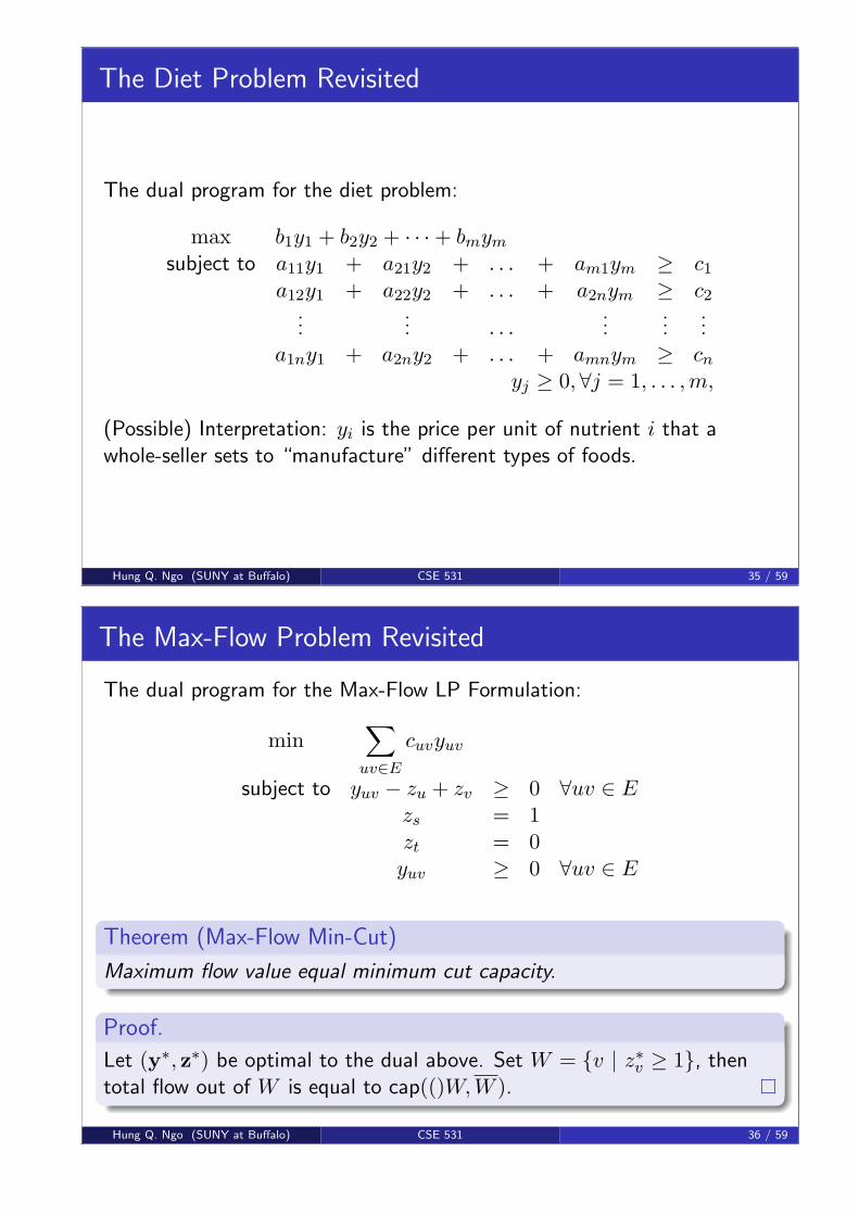
Strong Duality
Theorem (Strong Duality)
If the primal LP has an optimal solution x∗, then the dual LP has anoptimal solution y∗ such that
cTx∗ = bTy∗.
DualFeasible Infeasible
Optimal Unbounded
Feasible Optimal X Nah NahPrimal Unbounded Nah Nah X
Infeasible Nah X X
Hung Q. Ngo (SUNY at Buffalo) CSE 531 34 / 59
The Diet Problem Revisited
The dual program for the diet problem:
max b1y1 + b2y2 + · · ·+ bmym
subject to a11y1 + a21y2 + . . . + am1ym ≥ c1
a12y1 + a22y2 + . . . + a2nym ≥ c2...
... . . ....
......
a1ny1 + a2ny2 + . . . + amnym ≥ cn
yj ≥ 0,∀j = 1, . . . ,m,
(Possible) Interpretation: yi is the price per unit of nutrient i that awhole-seller sets to “manufacture” different types of foods.
Hung Q. Ngo (SUNY at Buffalo) CSE 531 35 / 59
The Max-Flow Problem Revisited
The dual program for the Max-Flow LP Formulation:
min∑
uv∈E
cuvyuv
subject to yuv − zu + zv ≥ 0 ∀uv ∈ Ezs = 1zt = 0yuv ≥ 0 ∀uv ∈ E
Theorem (Max-Flow Min-Cut)
Maximum flow value equal minimum cut capacity.
Proof.
Let (y∗, z∗) be optimal to the dual above. Set W = {v | z∗v ≥ 1}, thentotal flow out of W is equal to cap(()W,W ).
Hung Q. Ngo (SUNY at Buffalo) CSE 531 36 / 59
The Simplex Method: High-Level Overview
Consider a linear program min{cTx | x ∈ P}, P is a polyhedron
1 Find a vertex of P , if P is not empty (the LP is feasible)2 Find a neighboring vertex with better cost
If found, then repeat step 2Otherwise, either report unbounded or optimal solution
Hung Q. Ngo (SUNY at Buffalo) CSE 531 38 / 59
Questions
1 When is P not empty?
2 When does P have a vertex? (i.e. P is pointed)
3 What is a vertex, anyhow?
4 How to find an initial vertex?
5 What if no vertex is optimal?
6 How to find a “better” neighboring vertex
7 Will the algorithm terminate?
8 How long does it take?
Hung Q. Ngo (SUNY at Buffalo) CSE 531 39 / 59
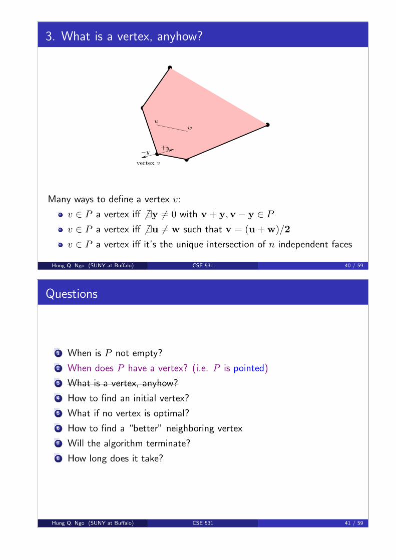
3. What is a vertex, anyhow?
vertex v
+y
uw
−y
Many ways to define a vertex v:
v ∈ P a vertex iff 6 ∃y 6= 0 with v + y,v − y ∈ P
v ∈ P a vertex iff 6 ∃u 6= w such that v = (u + w)/2v ∈ P a vertex iff it’s the unique intersection of n independent faces
Hung Q. Ngo (SUNY at Buffalo) CSE 531 40 / 59
Questions
1 When is P not empty?
2 When does P have a vertex? (i.e. P is pointed)
3 What is a vertex, anyhow?
4 How to find an initial vertex?
5 What if no vertex is optimal?
6 How to find a “better” neighboring vertex
7 Will the algorithm terminate?
8 How long does it take?
Hung Q. Ngo (SUNY at Buffalo) CSE 531 41 / 59
2. When is P pointed?
Question
Define a polyhedron which has no vertex?
Lemma
P is pointed iff it contains no line
Lemma
P = {x | Ax = b,x ≥ 0}, if not empty, always has a vertex.
Lemma
v ∈ P = {x | Ax = b,x ≥ 0} is a vertex iff the columns of Acorresponding to non-zero coordinates of v are linearly independent
Hung Q. Ngo (SUNY at Buffalo) CSE 531 42 / 59
Questions
1 When is P not empty?
2 When does P have a vertex? (i.e. P is pointed)
3 What is a vertex, anyhow?
4 How to find an initial vertex?
5 What if no vertex is optimal?
6 How to find a “better” neighboring vertex
7 Will the algorithm terminate?
8 How long does it take?
Hung Q. Ngo (SUNY at Buffalo) CSE 531 43 / 59
5. What if no vertex is optimal?
Lemma
Let P = {x | Ax = b,x ≥ 0}. If min{cTx | x ∈ P
}is bounded (i.e. it
has an optimal solution), then for all x ∈ P , there is a vertex v ∈ P suchthat cTv ≤ cTx.
Theorem
The linear program min{cTx | Ax = b,x ≥ 0} either
1 is infeasible,
2 is unbounded, or
3 has an optimal solution at a vertex.
Hung Q. Ngo (SUNY at Buffalo) CSE 531 44 / 59
Questions
1 When is P not empty?
2 When does P have a vertex? (i.e. P is pointed)
3 What is a vertex, anyhow?
4 How to find an initial vertex?
5 What if no vertex is optimal?
6 How to find a “better” neighboring vertex
7 Will the algorithm terminate?
8 How long does it take?
Hung Q. Ngo (SUNY at Buffalo) CSE 531 45 / 59
6. How to find a “better” neighboring vertex
The answer is the core of the Simplex method
This is basically one iteration of the method
Consider a concrete example:
max 3x1 + 2x2 + 4x3
subject to x1 + x2 + 2x3 ≤ 42x1 + 3x3 ≤ 54x1 + x2 + 3x3 ≤ 7
x1, x2, x3 ≥ 0.
Hung Q. Ngo (SUNY at Buffalo) CSE 531 46 / 59
Sample execution of the Simplex algorithm
Converting to standard form
max 3x1 +2x2 +4x3
subject to x1 +x2 +2x3 +x4 = 42x1 +3x3 +x5 = 54x1 +x2 +3x3 +x6 = 7
x1, x2, x3, x4, x5, x6 ≥ 0.
x =[0 0 0 4 5 7
]Tis a vertex!
Define B = {4, 5, 6}, N = {1, 2, 3}.The variables xi, i ∈ N are called free variables.
The xi with i ∈ B are basic variables.
How does one improve x? Increase x3 as much as possible! (x1 or x2
works too.)
Hung Q. Ngo (SUNY at Buffalo) CSE 531 47 / 59
Sample execution of the Simplex algorithm
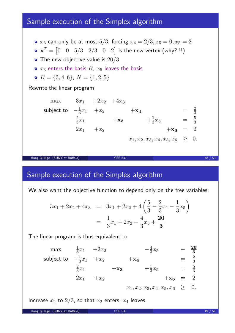
x3 can only be at most 5/3, forcing x4 = 2/3, x5 = 0, x5 = 2xT =
[0 0 5/3 2/3 0 2
]is the new vertex (why?!!!)
The new objective value is 20/3x3 enters the basis B, x5 leaves the basis
B = {3, 4, 6}, N = {1, 2, 5}
Rewrite the linear program
max 3x1 +2x2 +4x3
subject to −13x1 +x2 +x4 = 2
323x1 +x3 +1
3x5 = 53
2x1 +x2 +x6 = 2
x1, x2, x3, x4, x5, x6 ≥ 0.
Hung Q. Ngo (SUNY at Buffalo) CSE 531 48 / 59
Sample execution of the Simplex algorithm
We also want the objective function to depend only on the free variables:
3x1 + 2x2 + 4x3 = 3x1 + 2x2 + 4(
53− 2
3x1 −
13x5
)=
13x1 + 2x2 −
43x5 +
203
The linear program is thus equivalent to
max 13x1 +2x2 −4
3x5 + 203
subject to −13x1 +x2 +x4 = 2
323x1 +x3 +1
3x5 = 53
2x1 +x2 +x6 = 2
x1, x2, x3, x4, x5, x6 ≥ 0.
Increase x2 to 2/3, so that x2 enters, x4 leaves.
Hung Q. Ngo (SUNY at Buffalo) CSE 531 49 / 59
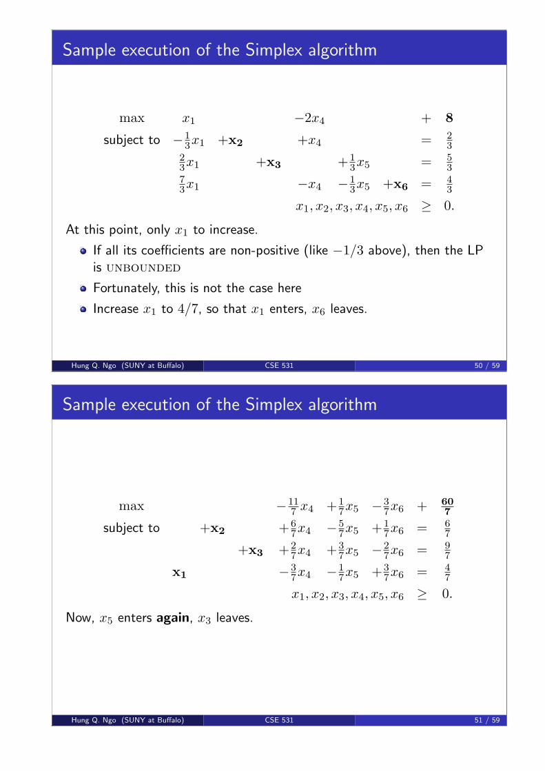
Sample execution of the Simplex algorithm
max x1 −2x4 + 8
subject to −13x1 +x2 +x4 = 2
323x1 +x3 +1
3x5 = 53
73x1 −x4 −1
3x5 +x6 = 43
x1, x2, x3, x4, x5, x6 ≥ 0.
At this point, only x1 to increase.
If all its coefficients are non-positive (like −1/3 above), then the LPis unbounded
Fortunately, this is not the case here
Increase x1 to 4/7, so that x1 enters, x6 leaves.
Hung Q. Ngo (SUNY at Buffalo) CSE 531 50 / 59
Sample execution of the Simplex algorithm
max −117 x4 +1
7x5 −37x6 + 60
7
subject to +x2 +67x4 −5
7x5 +17x6 = 6
7
+x3 +27x4 +3
7x5 −27x6 = 9
7
x1 −37x4 −1
7x5 +37x6 = 4
7
x1, x2, x3, x4, x5, x6 ≥ 0.
Now, x5 enters again, x3 leaves.
Hung Q. Ngo (SUNY at Buffalo) CSE 531 51 / 59
Sample execution of the Simplex algorithm
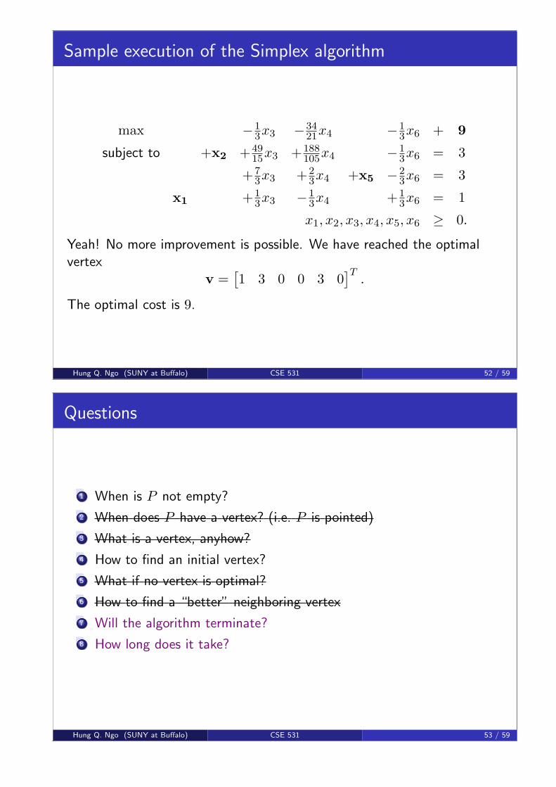
max −13x3 −34
21x4 −13x6 + 9
subject to +x2 +4915x3 +188
105x4 −13x6 = 3
+73x3 +2
3x4 +x5 −23x6 = 3
x1 +13x3 −1
3x4 +13x6 = 1
x1, x2, x3, x4, x5, x6 ≥ 0.
Yeah! No more improvement is possible. We have reached the optimalvertex
v =[1 3 0 0 3 0
]T.
The optimal cost is 9.
Hung Q. Ngo (SUNY at Buffalo) CSE 531 52 / 59
Questions
1 When is P not empty?
2 When does P have a vertex? (i.e. P is pointed)
3 What is a vertex, anyhow?
4 How to find an initial vertex?
5 What if no vertex is optimal?
6 How to find a “better” neighboring vertex
7 Will the algorithm terminate?
8 How long does it take?
Hung Q. Ngo (SUNY at Buffalo) CSE 531 53 / 59
7&8 Termination and Running Time
Termination
There are finitely many vertices (≤(
nm
))
Terminating = non-cycling, i.e. never come back to a vertex
Many cycling prevention methods: perturbation method,lexicographic rule, Bland’s pivoting rule, etc.
Bland’s pivoting rule: pick smallest possible j to leave the basis, thensmallest possible i to enter the basis
Running time
Klee & Minty (1969) showed that Simplex could take exponential time
Hung Q. Ngo (SUNY at Buffalo) CSE 531 54 / 59
Summary: Simplex with Bland’s Rule
1 Start from a vertex v of P .
2 Determine B and N ; Let yTB = cT
BA−1B .
3 If(cTN − yT
Baj
)≥ 0, then vertex v is optimal. Moreover,
cTv = cTBvB + cT
NvN = cTB
(A−1
B b−A−1B ANvN
)+ cT
NvN
4 Else, letj = min
{j′ ∈ N :
(cj′ − yT
Baj′)
< 0}
.
5 If A−1B aj ≤ 0, then report unbounded LP and Stop!
6 Otherwise, pick smallest k ∈ B such that(A−1
B aj
)k
> 0 and that
(A−1B b)k(
A−1B aj
)k
= min
{(A−1
B b)i(A−1
B aj
)i
: i ∈ B,(A−1
B aj
)i> 0
}.
7 xk leaves, xj enters: B = B ∪ {j} − {k}, N = N ∪ {k} − {j}.Go back to step 3.
Hung Q. Ngo (SUNY at Buffalo) CSE 531 55 / 59
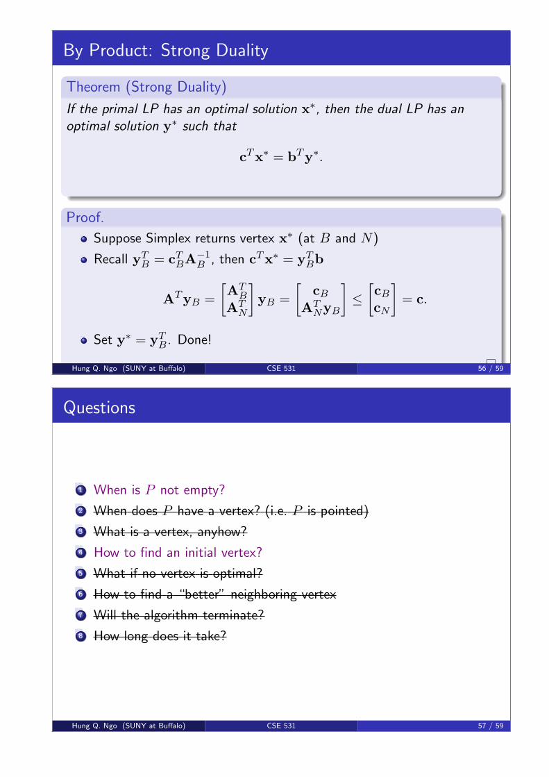
By Product: Strong Duality
Theorem (Strong Duality)
If the primal LP has an optimal solution x∗, then the dual LP has anoptimal solution y∗ such that
cTx∗ = bTy∗.
Proof.
Suppose Simplex returns vertex x∗ (at B and N)
Recall yTB = cT
BA−1B , then cTx∗ = yT
Bb
ATyB =[AT
B
ATN
]yB =
[cB
ATNyB
]≤
[cB
cN
]= c.
Set y∗ = yTB. Done!
Hung Q. Ngo (SUNY at Buffalo) CSE 531 56 / 59
Questions
1 When is P not empty?
2 When does P have a vertex? (i.e. P is pointed)
3 What is a vertex, anyhow?
4 How to find an initial vertex?
5 What if no vertex is optimal?
6 How to find a “better” neighboring vertex
7 Will the algorithm terminate?
8 How long does it take?
Hung Q. Ngo (SUNY at Buffalo) CSE 531 57 / 59
1&4 Feasibility and the Initial Vertex
In P = {x | Ax = b,x ≥ 0}, we can assume b ≥ 0 (why?).
Let A′ =[A I
]Let P ′ = {z | A′z = b, z ≥ 0}.A vertex of P ′ is z = [0, . . . , 0, b1, . . . , bm]T
P is feasible iff the following LP has optimum value 0
min
{m∑
i=1
zn+i | z ∈ P ′
}
From an optimal vertex z∗, ignore the last m coordinates to obtain avertex of P
Hung Q. Ngo (SUNY at Buffalo) CSE 531 58 / 59
Questions
1 When is P not empty?
2 When does P have a vertex? (i.e. P is pointed)
3 What is a vertex, anyhow?
4 How to find an initial vertex?
5 What if no vertex is optimal?
6 How to find a “better” neighboring vertex
7 Will the algorithm terminate?
8 How long does it take?
Hung Q. Ngo (SUNY at Buffalo) CSE 531 59 / 59