Agency, Firm Growth, and Managerial Turnover∗

Ronald W. Anderson†, Cecilia Bustamante‡and Stephane Guibaud§

November 18, 2011

Abstract

This paper analyzes the relation between firm growth and managerial incentiveprovision in a dynamic moral hazard environment. We characterize the optimal growth,firing and compensation policies specified in the long-term contracts signed between aninfinitely-lived firm and the managers who sequentially run the firm. We show that therealized growth of firms depends both on the exogenous arrival of growth opportunitiesand the severity of moral hazard. Managerial turnover arises upon poor managerialperformance to provide incentives, but can also be induced by growth when firms find itmore profitable to grow with a new manager. Contracts rely on deferred compensationas a means of incentivizing agents; however, firms with better investment opportunitiesrely on more front-loaded compensation. We also identify a new component of agencycosts which relates exclusively to managerial turnover, and relates to the spillover effectof the length of an existing managerial contract onto the present value of all futurecontracts signed by the firm.

1 Introduction

Firms extract value not only from operating their existing assets, but also from theexpected future profits of their growth opportunities. The latter source of value creationtypically involves implementing major changes of strategy, exploring new markets,developing new products, adopting innovative production techniques or changing theorganization of labor within the firm. However incumbent managers, for a variety ofreasons, may lack the vision or the skills that are necessary to lead the firm througha new growth phase. Firms often find that major management changes are needed topursue their growth opportunities successfully.

This paper explores how growth-induced management turnover interacts with theprovision of managerial incentives in a dynamic moral hazard model. We consider a

∗Preliminary draft. Comments welcome. We are grateful to Mike Fishman and seminar participants atLSE for their comments. All responsibility for errors and views expressed is our own.

†London School of Economics, r.w.anderson@lse.ac.uk‡London School of Economics, m.bustamante@lse.ac.uk§London School of Economics, s.guibaud@lse.ac.uk

1

firm with assets in place and growth opportunities, which is run by a sequence of man-agers throughout its life-cycle. As in previous studies on optimal long term contractswith limited liability, firms can use the threat of early termination to discipline theirincumbent managers, i.e., firms often fire their managers after periods of poor perfor-mance. But in contrast with previous studies, our paper stresses that firms may alsofire their managers despite good performance if a change of management is the best oronly option to seize valuable growth opportunities.

In our model, a risk-neutral manager is hired by a risk neutral, long-lived firm to runits existing assets. Cash flows are only observable by the manager, who can then under-report and divert them for his own private benefit. The firm can fire its incumbentmanager at any point in time, and replace him at a cost. Growth opportunities arestochastic and may arrive in any period. We assume that growth is efficient underfirst-best and investment is contractible. In our baseline model, the firm needs toreplace its current manager in order to pursue a growth opportunity. We later showthat growth-driven turnover arises endogenously when it is more profitable for a firmto grow with a new manager. Upon taking up a growth opportunity, the firm pays thecosts of investing and replacing the manager, and the scale of its business increases.

We solve for the optimal long-term contract signed between the firm and each ofits successive managers at the time they are hired. As in other papers in the literatureon dynamic moral hazard, a manager’s expected discounted payoff under the optimalcontract, or continuation value, evolves over time and its sensitivity to cashflows isrelated to the severity of the agency problem. A key feature in our analysis is that thecontinuation value of the firm upon replacing an incumbent manager is endogenous(equal to the value of the firm under the newly hired manager), and contingent onthe current availability of a growth opportunity. This contrasts with most of theexisting dynamic contracting models where, upon firing the manager, the firm obtainsan exogenously given liquidation value.

Our results in the baseline model are as follows. First, the realized growth of firmsdepends both on the technological features of the growth process and on the severityof moral hazard. That is, a firm’s corporate governance can be a key determinant ofcorporate growth. In our model, two firms with similar growth opportunities may endup having very different realized growth profiles just because they differ in the severityof the agency problem they face. A firm plagued with more severe agency problem mayforego a growth opportunity and decide instead to retain its incumbent management,when the growth opportunity arises after a period of good performance. Throughoutthe paper, we therefore distinguish between two (endogenous) types of firms: lowgrowth firms that may or may not undertake growth opportunities depending upon thepast performance of the incumbent manager, and high growth firms that undertake allgrowth opportunities when they arise. In the former type of firms, underinvestmentadds to the usual inefficiency that, for the sake of ex ante incentive provision, managerscan be fired upon poor past performance in the absence of a growth opportunity.

Second, the probability of replacing an incumbent manager in our model dependsnot only on past and current performance, as summarized by the manager’s continua-tion value, but also on the availability of a growth opportunity. In all firms, the con-ditional probability of managerial replacement is higher in states of the world where

2

a growth opportunity is available. In low growth firms, the performance thresholdbeing used to determine replacement decision is set at a higher level in these states,making replacement more likely. In high growth firm, the incumbent management issystematically replaced when a growth opportunity arises.

Third, we find that the optimal compensation scheme is readily implementableby a system of deferred compensation credit, bonuses and severance pay. Deferredcompensation is used, along with the threat of inefficient replacement, in order toprovide incentives in the best possible way. We show that the degree to which firmsrely on back-loading of compensation is affected by their growth prospects. Namely,the extent of back-loading decreases with the quality of firms’ growth opportunities.

Lastly, we identify a new component of agency costs that arises in our framework,which is due to a form of contractual externality. When a firm offers a contract to anewly hired manager, it fails to take into account the spillover effect upon the expectedamount of time before hiring future managers and thus the present value of compen-sation received by all future managers. The agency cost induced by this externality isnaturally larger for low growth firms, where the arrival of a growth opportunity doesnot always result in managerial turnover. This externality of the current binding con-tracts of the firm on its future binding contracts does not arise in earlier papers in theliterature, in which firms are liquidated at an exogenous value upon termination of theincumbent, and only, manager of the firm.

In an extension of the baseline model, we allow firms to grow with their incumbentmanagers, possibly at a different cost than when they grow with a new manager. When-ever it is sufficiently more costly to grow with the incumbent manager, e.g., becauserealizing a growth opportunity would require paying an army of external consultantsto help the firm reinvent itself, all the results of the baseline model survive. However,under symmetric costs, an alternative set of predictions emerges. When the costs ofgrowth are reasonably low, firms always undertake their growth opportunities, some-times with their incumbent managers. Managers are only fired upon poor performance,but it is still the case that the performance threshold that determines the probabilityof replacement is higher when a growth opportunity is available.

Our paper relates to several strands in the finance and economics literature on dy-namic contracting and the theory of the firm. The works by Quadrini (2004), Clementiand Hopenhayn (2006), DeMarzo and Fishman (2007a), Biais et al. (2010), DeMarzo etal. (2011), and Philippon and Sannikov (2011) explore, as we do, the link between dy-namic moral hazard and contractible investment opportunities.1 Our framework differsfrom these papers in several dimensions. The key difference is that in our frameworkgrowth may entail replacing the current manager; whereas, all of the papers mentionedassume that a firm retains the same manager over its entire life-cycle. Furthermore,in contrast with Quadrini (2004), Clementi and Hopenhayn (2006), and DeMarzo andFishman (2007a), we endogenize the liquidation value of the firm, and focus on man-agerial turnover rather than firm survival. Finally, in contrast with DeMarzo andFishman (2007a) and DeMarzo et al. (2011), we consider growth opportunities whicharrive stochastically.

1He (2008) considers an environment where growth is affected by non-observable effort.

3

Our paper relates to Spear and Wang (2005), who develop a dynamic contractingmodel where a firm can fire the incumbent manager, and hire a new one from anexternal labor market. Spear and Wang (2005) do not account for growth opportunitiesin their setup. Consequently, the economic determinants of managerial turnover in theirmodel differ from the ones emphasized in our paper.

Our notion that the growth of a firm may require replacing the incumbent manageris found in many early contributions to the managerial theory of the firm. Penrose(1959) discusses why firms may operate successfully under competent managers butmay still fail to take full advantage of their opportunities of expansion. Williamson(1966) elaborates on how management constraints affect the realized growth of firms.More recently, Roberts (2004) echoes Penrose by emphasizing the need for differentorganizational capabilities in the exploration and exploitation of firms’ investmentprojects. He discusses a number of business cases where this effect if prominent. Intheir empirical study of U.S. firms, Murphy and Zimmerman (1993) study a varietyof measures of firm performance in the years preceding and following CEO turnover.They report a decline in capital expenditures in the year of CEO replacement followedby a sharp increase subsequently. In their theoretical analysis using a repeated moralhazard framework but without optimal contracting, Anderson and Nyborg (2011) showthe link between managerial replacement and firm growth are affected the firm’s choiceof debt or equity financing.

Finally, our paper relates to the empirical literature that highlights how managerialturnover and incentives relate to realized growth. In the context of venture capital,Kaplan, Sensoy and Stromberg (2009) find that the management team of firms in theirearly stages of growth firms undergo high turnover before the IPO. This is consistentwith the prediction in our model that firms with high realized growth have high man-agerial turnover. The testable implications of our model on managerial turnover andgrowth also relate to the recent study by Jenter and Lewellen (2011) on CEO turnoverand acquisitions. As in this paper, acquisitions are major investments in which tar-get CEOs are either fired or forced to retire early; Jenter and Lewellen (2011) thenshow that all else equal takeovers are more likely when incumbent CEOs reach theirretirement age and hence it is cheaper to replace them.

The paper proceeds as follows. Section 2 describes the model. Section 3 derives theoptimal long-term contract, and provides an informal discussion of its main features.Section 4 provides an illustration in the stationary limit of the model. Section 5 employsnumerical simulations to further analyze the implications of our model and quantifythe effects. Section 6 extends our results to an alternative environment where the firmcan grow with its current manager. All proofs are relegated in a separate Appendix.

2 The model

2.1 Setup

Time is discrete. We consider a project/firm that generates a stream of risky cashflows{Y1, Y2, ..., YT } over T periods (we later consider the stationary limit as T goes to

4

infinity). The project is run by an agent (the manager) who can underreport cashflowsand divert them for his own private benefit. We assume that the agent gets λ ≤ 1 foreach unit of diverted cash, so that λ captures the severity of moral hazard. In anyperiod, an incumbent agent can be fired (at some cost) and replaced by a new agent.For simplicity, we assume that the value of an agent’s best outside option upon beingfired is zero.

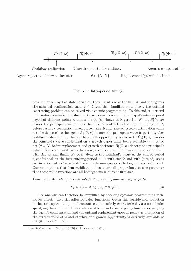
The firm cashflow in period t is Yt = Φtyt, where Φt is the size of the firm at thebeginning of period t and yt is iid with support Y, minY = 0, and E(yt) = µ forall t. The firm size Φ evolves over time according to the stochastic arrival of growthopportunities. In each period, with probability q and independently from currentcashflow realization, the firm gets a chance to grow at rate γ. The state variable θcaptures the availability of a growth opportunity in a given period, where θ = G withprobability q and θ = N with probability 1 − q. We assume that taking up a growthopportunity involves paying some investment cost and hiring a new manager (we relaxthe latter assumption in Section 6). If a growth opportunity materializes in period t,given an initial size Φt, the firm can grow to a size (1+γ)Φt in period t+1 at a cost of(χ+κ)Φt, where χ and κ denote the proportional costs of scaling-up and replacing themanager, respectively. Otherwise, if there is no growth opportunity or if an availablegrowth opportunity is not taken up, the size of the firm remains constant. In case nogrowth opportunity is available it still is possible to replace the manager at cost κΦt.Figure 1 summarizes the timing within each period.

The assumption that growth necessarily entails replacing the incumbent managercaptures the idea that the growth described by the model requires a new skill setand/or a change in corporate culture. The incumbent manager, whose human capitalhas to some degree become specific to the firm in its current form during his tenure,will have lost the flexibility to adapt his skills to new requirements. While we havein mind drastic changes of the firm, as a modeling convenience we capture this as adiscrete change of scale of the firm, as indicated by the rate of cashflows. However,growth in our context may not involve an increase in physical capital. Instead growthcould even be thought of as simply the result of finding better managers.

Agents and principal are risk-neutral with (continuously compounded) discountrates ρ and r, respectively, with ρ > r. When considering the stationary limit of themodel as T → ∞, we impose that qγ < er − 1 (i.e., the average growth rate is lowerthan the principal’s discount rate) to ensure finite valuation.

We assume that the (proportional) replacement cost κ is independent of whethera growth opportunity is available or not. Because of this cost, it would be inefficientto fire and replace an incumbent agent under first best, absent a growth opportunity.However, we assume that it is efficient to replace management to take up an availablegrowth opportunity, which in the infinite horizon limit of the model amounts to thefollowing parameter restriction

γµ

er − 1> κ + χ. (1)

As a benchmark, it is useful to consider the value of the firm in the case of symmetricinformation about cashflows. Under condition (1), the optimal firm policy involves

5

taking up all available growth opportunities and firing managers only upon growth.Let Vt(Φ) denote the first-best value of the firm (ex-cashflow) in period t, before thegrowth opportunity realization. The sequence of first-best value functions is givenrecursively by

Vt(Φ) = q[

−(κ + χ)Φ + e−r {(1 + γ)Φµ + Vt+1[(1 + γ)Φ]}]

+ (1 − q)e−r{Φµ + Vt+1(Φ)},

where the recursion starts at VT (Φ) = 0, for all Φ. The homogenous nature of themodel allows us, in the infinite horizon limit, to write V (Φ) = v∗Φ, where

v∗ =−q(κ + χ) + e−r(1 + qγ)µ

1 − e−r(1 + qγ). (2)

2.2 Contracting

We now consider optimal second best contracting under asymmetric information. Acontract is established between the investor and the manager at the outset of his tenure.When the latter is replaced, the contract is terminated and a new contract is estab-lished with a new manager. In the case of asymmetric information about cashflows, acontract specifies as a function of history (i.e., the sequence of payments received by theprincipal, as well as the history of growth opportunity realizations), circumstances un-der which an agent is fired (i.e., history-contingent firing probabilities), investment andgrowth, and non-negative cash compensation from principal to agents. For simplicity,we assume a contractual environment with full-commitment (no renegotiation) and weassume that the agent cannot save, and therefore consumes in each period his currentcompensation plus the diverted cashflow.2 The amount of diversion is the only decisionover which the agent has control. In searching for an optimal contract, we restrict ourattention to contracts that induce truthful reporting (indeed, since λ ≤ 1 diversion isat least weakly inefficient). An optimal contract is one that satisfies the associatedincentive-compatibility constraint and gives the maximum payoff to the principal sub-ject to providing a certain payoff to the agent. For now, we assume that the contractis designed so as to give an expected discounted value of Φw0 to a manager hired torun the firm at size Φ.

3 The optimal contract

In this section, we characterize managerial compensation, managerial turnover, andrealized firm growth under the optimal contract. Our derivation of the optimal contractfollows the recursive approach pioneered by Green (1987) and Spear and Srivastava(1987). Let w denote the size-adjusted continuation value of the current manager (i.e.,for current size Φ, the agent’s continuation value is Φw). In our context, history can

2The assumption that the agent cannot engage in private saving is not crucial. What is required is thatthe rate of return available to the agent is less than or equal to r, i.e., private saving is weakly inefficient.Under this condition, even if allowed to do so, the agent would have no incentive to use private savings underthe derived optimal contract. See DeMarzo and Fishman (2007b), Section 2.1 and Corollary 1.

6

-

Byt (Φ, w)

6

Cashflow realization.

Agent reports cashflow to investor.

Bqt (Φ, w)

6

Growth opportunity realizes.

θ ∈ {G, N}.

Bℓt,θ(Φ, w)

6

Replacement/growth decision.

Bct (Φ, w)

6

Agent’s compensation.

Bet (Φ, w)

Figure 1: Intra-period timing

be summarized by two state variables: the current size of the firm Φ, and the agent’ssize-adjusted continuation value w.3 Given this simplified state space, the optimalcontracting problem can be solved via dynamic programming. To this end, it is usefulto introduce a number of value functions to keep track of the principal’s intertemporalpayoff at different points within a period (as shown in Figure 1). We let By

t (Φ, w)denote the principal’s value under the optimal contract at the beginning of period t,before cashflow realization, given current size Φ and (size-adjusted) continuation valuew to be delivered to the agent; Bq

t (Φ, w) denotes the principal’s value in period t, aftercashflow realization, but before the growth opportunity is realized; Bℓ

t,θ(Φ, w) denotesthe principal’s value conditional on a growth opportunity being available (θ = G) ornot (θ = N) before replacement and growth decisions; Bc

t (Φ, w) denotes the principal’svalue before compensation to the agent, conditional on the firm entering period t + 1with size Φ; and finally Be

t (Φ, w) denotes the principal’s value at the end of periodt, conditional on the firm entering period t + 1 with size Φ and with (size-adjusted)continuation value eρw to be delivered to the manager as of the beginning of period t+1.Our assumptions that firm cashflows and costs are all proportional to size guaranteethat these value functions are all homogenous in current firm size.

Lemma 1. All value functions satisfy the following homogeneity property

Bt(Φ, w) = ΦBt(1, w) ≡ Φbt(w). (3)

The analysis can therefore be simplified by applying dynamic programming tech-niques directly onto size-adjusted value functions. Given this considerable reductionin the state space, an optimal contract can be entirely characterized via a set of rulesspecifying the evolution of the state variable w, and a set of policy functions specifyingthe agent’s compensation and the optimal replacement/growth policy as a function ofthe current value of w and of whether a growth opportunity is currently available ornot (θ = G or θ = N).

3See DeMarzo and Fishman (2007a), Biais et al. (2010).

7

3.1 Properties of the optimal contract

We solve for the size-adjusted value functions, the law of motion for the agent’s contin-uation value w, along with the optimal compensation, growth and replacement policiesby backward induction, along the lines of DeMarzo and Fishman (2007b). The recur-sion starts in the final period with bℓ

T,θ(w) = −w for θ = G,N . Now suppose bℓt+1,G(w)

and bℓt+1,N (w) are known. Then

bqt+1(w) = qbℓ

t+1,G(w) + (1 − q)bℓt+1,N (w), (4)

which is simply an expectation over the realization of θ in period t+1. The beginning-of-period value function is obtained as

byt+1(w) = max

{wq(y)}y∈Y

µ + E{bqt+1[w

q(y)]}, (5)

where the expectation is taken over the distribution of y, subject to promise-keepingcondition E[wq(y)] = w, limited liability wq(y) ≥ 0, and incentive-compatibility con-straint

wq(y) ≥ wq(y) + λ(y − y), ∀y ∈ Y, ∀y ∈ [0, y]. (6)

The following lemma further characterizes the beginning-of-period value function, aswell as the cashflow sensitivity of the agent’s updated continuation value.

Lemma 2. In any period t, byt is only defined for w ≥ λµ. Moreover,

wq(y,w) = w + λ(y − µ), w ≥ λµ. (7)

The intuition behind Eq. (7) is that in order to induce the agent not to divert, hiscontinuation value must have a sensitivity λ to his payment to the principal. Hencethe incentive-compatibility condition gives the slope of wq with respect to y, whilethe promise-keeping condition gives the level of the schedule. The fact that by

t is onlydefined for w ≥ λµ comes from the limited liability constraint: indeed, w needs tobe high enough to guarantee that even for the lowest possible cashflow realization(minY = 0), the continuation value wq(y) consistent with incentive-compatibility andpromise-keeping constraints remains non-negative. Given by

t+1, the end-of-period valuefunction in period t is simply given by

bet (w) = e−rby

t+1(eρw), w ≥ e−ρλµ, (8)

where the domain of bet follows directly from that of by

t+1.

Lemma 3. For t < T − 1, bet is concave in w.

In a Modigliani-Miller world, increasing the agent’s value would merely amountto redistributing total firm value, and the principal’s value would simply be linearlydecreasing in the agent’s value with a slope of −1. In the presence of moral hazard,costly replacement and firm growth, a change in w also affects the principal’s value

8

via its impact on the likelihood of inefficient firing. Under the contract the investoris committed to firing the agent following a string of bad cash flow realizations eventhough this may be costly (i.e., ex post inefficient) for the investor. When the manager’scurrent promise is low, this ex post bad outcome for the investor is relatively likely.Increasing the agent’s promise by some given amount hurts the investor by sacrificingsome portion of future cash flows, but this is mitigated by the fact that it reduces theprospect of a costly turnover. When the manager’s current promise is relatively high,the prospect of turnover is slight and the benefit derived from reducing it is also slight.4

3.1.1 Cash compensation

The value function bct captures the principal’s value contingent on the incumbent man-

ager being retained. The problem at this stage is to find the best possible way tocompensate the agent over time, by employing the optimal mix of present versus fu-ture compensation. Formally, for w ≥ e−ρλµ

bct(w) = max

c,we−c + be

t (we) (9)

subject to the promise keeping condition c + we = w, the limited liability conditionc ≥ 0 and we ≥ e−ρλµ.

Lemma 4. Let wt such that bet′(wt) = −1. The optimal compensation policy is

ct(w) =

{

0, w ≤ wt,w − wt, w > wt.

(10)

Therefore, bct(w) = be

t (w) for w ≤ wt and bct(w) = be

t (wt) − (w − wt) for w > wt.

Lemma 4 states that it is optimal to defer an agent’s compensation until his con-tinuation value has reached the threshold wt. The optimal compensation threshold isdetermined by a basic tradeoff: delayed compensation is preferable because it keeps theagent’s promise from falling closer to the inefficient termination threshold, while earlycompensation is preferable because the agent is more impatient than the principal.Formally, the compensation threshold wt is determined by comparing the marginalcost for the principal of present versus deferred compensation. By compensating theagent with ∆c in period t, the principal’s value is −∆c + be

t (w − ∆c). For a small∆c, this can be approximated by be

t (w)−∆c(−1− bet′(w)), which shows that non-zero

compensation is optimal if and only if bet′(w) < −1.

3.1.2 Replacement and growth

We can now proceed with the construction of bℓt,θ for θ = G,N , which will end the

recursion. At this stage, given the realization of θ and the manager’s continuationvalue w, the contract specifies firing probability pt,θ(w), severance pay st,θ(w), and the

4Note that an increase in w can also affect the growth prospects of the firm, as will become clear fromProposition 1.

9

updated continuation value wct,θ(w) that the incumbent manager would get upon being

retained. Note that if θ = N , the principal’s continuation value (adjusted by currentsize) upon replacing the incumbent manager is:

ℓt,N = e−rbyt+1(w0) − κ. (11)

If instead a growth opportunity is available in period t, the principal’s continuationvalue upon firing the incumbent manager would be

ℓt,G = max{e−r(1 + γ)byt+1(w0) − (κ + χ); e−rby

t+1(w0) − κ}, (12)

where the second term corresponds to the case where the incumbent manager is firedbut the growth opportunity is not undertaken. For economically interesting cases, itis reasonable to assume that replacing the manager is more valuable when there isa growth opportunity than when there is not. It follows that ℓt,G > ℓt,N . Then wecan interpret pt,G(w) as the the conditional probability of growing contingent on agrowth opportunity being available. Informally, we can think of this as the conditionalprobability of efficient replacement (i.e., conditional on θ = G). Similarly, pt,N (w)captures the conditional probability of inefficient firing.

The optimal severance and replacement/growth policies are obtained by consideringthe following constrained maximization problem, separately for θ = G and θ = N :

bℓt,θ(w) = max

p,s,wcp(ℓt,θ − s) + (1 − p)bc

t(wc) (13)

subject to the promise keeping condition ps + (1 − p)wc = w, the limited liabilitycondition s ≥ 0, wc ≥ e−ρλµ, and p ∈ [0, 1]. To analyze this problem, it is useful tointroduce for θ = G,N

δt,θ = sup

{

bct(w) − ℓt,θ

w: w ≥ e−ρλµ

}

, (14)

and

wt,θ =

{

inf{w ≥ e−ρλµ : bct′(w) ≤ δt,θ}, if δt,θ > −1,

∞, otherwise.(15)

Graphically, δt,θ and wt,θ are determined by finding the line of maximum slope relatingthe termination point (0, ℓt,θ) to the curve representing bc

t(w). The slope of this linegives δt,θ, while wt,θ is defined as the value of w at the intersection/tangency pointif δt,θ > −1 and wt,θ = ∞ otherwise. Note that (14) along with ℓt,G > ℓt,N impliesδt,G < δt,N .

Proposition 1. For any realization of θ ∈ {G,N}, the optimal replacement policy canbe described as follows:

(i) if δt,θ > −1, the probability of the incumbent agent being replaced is

pt,θ(w) =

{

1 − w/wt,θ, 0 ≤ w < wt,θ,

0, w ≥ wt,θ.(16)

10

The agent receives no severance pay upon being fired, st,θ(w) = 0, ∀w < wt,θ, andhis continuation value upon being retained is

wct,θ(w) =

{

wt,θ, 0 < w < wt,θ,

w, w ≥ wt,θ,(17)

Hence

bℓt,θ(w) =

{

ℓt,θ + δt,θw, 0 ≤ w ≤ wt,θ,

bct(w), w ≥ wt,θ.

(18)

(ii) if δt,θ ≤ −1, the incumbent manager is replaced with probability one independentlyof the agent’s promised value, pt,θ(w) = 1 for all w ≥ 0. Upon being replaced, themanager receives st,θ(w) = w, and

bℓt,θ(w) = ℓt,θ − w, ∀w ≥ 0. (19)

3.2 Implementation of the optimal contract

Having formally derived the optimal contract in our setting, it is useful to summarize itinformally and to discuss how it can be implemented in practice. The optimal contractbetween the firm and its manager sets out the conditions under which the managerwill be compensated during his tenure at the firm and also those which will lead tohis leaving the firm. These terms and conditions are chosen to maximize the value ofpayoffs to the firm’s owners subject to incentivizing the manager to truthfully reportrealized cashflows. Payments and retention/replacement decisions are made over timeas a function of the value of promised deferred payments, wt, which evolves under theinfluence of the firm’s operating performance and changing growth opportunities. Thecontractual features in force at time t are summarized in three threshold values wt,wt,G, and wt,N , and the manager receives qualitatively different treatment dependingupon whether wt is above or below these thresholds.

wt is the bonus threshold. In any period t following the realization and report of thefirm’s cashflows, yt, the manager’s promise is adjusted linearly according to Equation(7). The sensitivity of this promise to cashflow changes reflects the severity of agencyproblems faced by the firm. The more severe the agency problem, the greater shouldbe this sensitivity. If after adjustment the resulting promise lies above the bonusthreshold, (wt > wt), a bonus is awarded in that period equal to the excess, (wt −wt),and the agent’s continuing promise is reduced to the threshold amount, wt.

The other two threshold values may be thought of as replacement thresholds, and, asthe replacement decision is made after the availability of a growth opportunity (or lackthereof) has been observed, these thresholds are conditioned on such opportunity beingavailable or not. wt,N is the dismissal threshold when there is no growth opportunityavailable. If the manager’s current promise lies above this threshold, wt > wt,N , thenhe knows that he will be retained. In particular, if he has just been awarded a bonus,he is retained for sure when there is no growth opportunity (indeed, wt,N < wt).If rather the operating performance has been so poor that the manager’s promise isbelow the threshold, wt < wt,N , then he is at risk of being fired. In effect, he is given alottery whereby with some probability he will be dismissed and will receive no further

11

payments from the firm. If he survives this, he stays with the firm and is awardeda continuing promise that is increased to the dismissal threshold amount, wt = wt,N .The probability of dismissal is chosen so that this lottery is fair, i.e., its expected valueequals the agent’s promise following the report of cashflow.

For one type of firm the logic of the dismissal decision when the growth opportunityis available is similar to the above; however, it is made by comparing the promise tothe growth dismissal threshold wt,G which is higher than that without growth (i.e.,wt,G > wt,N ). That is, risk of dismissal weakly increases if a growth opportunityarises. If the manager’s promise is above the threshold wt,G he knows he is safe. If heis below this threshold he is given a fair lottery in which, if he is dismissed, he leavesthe firm with no further compensation, and, if he survives, he is given a continuingpromise which is increased to wt,G. However, this replacement rule does not apply inall firms. In a second type of firm, upon the arrival of the growth opportunity, themanager knows he will be dismissed for sure and upon leaving the firm will receive aseverance pay equal to his current promise, s = wt.

In light of these comments on the replacement decision in the face of growth, it isuseful to distinguish two categories of firms depending upon the attractiveness of theirgrowth opportunities. A high growth firm is one that will undertake growth any timeit has an opportunity, independently of the firm’s past operating performance. Otherfirms, which for simplicity we call low growth firms even though in practice they maygrow quite fast, do not always take up an available growth opportunity. Instead, theywill possibly retain the current manager and keep operating assets at the current scale,if past performance has been good enough and the manager has accumulated a highpromised compensation. Proposition 1 shows that the distinction between high andlow growth firms depends crucially on the quantities δt,G and δt,N defined by Eq. (14).Low growth firms are characterized by δt,N > δt,G > −1. High growth firms satisfyδt,N > −1 and δt,G ≤ −1. Whenever δt,θ ≥ −1, this quantity indicates the slope of thePareto frontier describing the firm owners’ value as a function of the value promisedto the current manager, as implied by the dismissal lotteries described above (i.e., forlow enough promised values). The slope of the frontier itself can never fall below −1,since the firm always has the option to pay cash immediately, in which case an increasein the manager’s promised value simply translates one-for-one into a reduced value forthe firm owners.5

High growth firms and low growth firms behave in dramatically different ways. Whilehigh growth firms always seize an opportunity to invest and grow, fully realizing theirgrowth potential, low growth firms do not systematically take up available growthopportunities, thus wasting part of their growth potential. Hence, for the latter firms,an important source of agency cost is under-investment. For low growth firms, theprobability of taking a growth opportunity, pt,G(w), is decreasing in w. That is, thebetter has been the operating performance recently, the less likely that the firm willtake up a growth opportunity. These firms do not take up growth opportunities for high

5Note that with a finite horizon T , the same firm can possibly switch type over its life-cycle. In Section4.3, we provide a mapping of high growth vs. low growth firms in the parameter space in the stationary limitof the model.

12

w because the overall cost of taking up the growth opportunity is too high. This resultcontrasts with DeMarzo and Fishman (2007a) who find that investment is increasingin the agent’s promise because the return on investment is high then.

In the absence of a growth opportunity, both types of firms have similar policies.Eq. (28) describes pt,N (w). The probability of replacement is positive and decreasingif and only if the promise is below the threshold, w < wt,N . Taken together withthe cashflow sensitivity of wq, this means that the probability of an agent being fired(conditional on θ = N) increases with bad (past and current) performance. Thisreplacement policy, combined with zero severance pay sN(w) = 0, is used as a threatto provide the right incentives to the agent while respecting limited liability. Note thatterminating the agent when θ = N is inefficient and contributes to the agency costsinduced by asymmetric information.

The optimal contract we have just described can be implemented fairly directlyusing standard employment contracts, and there is some evidence that features of ouroptimal contracts are used in practice. The bonus calculation in this contract is verymuch like the typical contract that was found by Murphy (2001) in his study of thebonus contracts of large U.S. firms in 1997. The key parameters he identifies are theperformance target, the pay-performance-sensitivity (pps), and the bonus threshold.In our contracts, these are µ, λ, and wt respectively.

Our contract specifies an indefinite term with both the manager and the firm havingthe right to terminate at will.6 Actual employment contracts are often written in thisway.7 In practice, it is not unheard of that following a period of poor performance whenthe manager was thought to be under threat of dismissal, the firm instead retains themanager and gives him an improved compensation package as a vote of confidence.This is analogous to the award of deferred compensation of wθ −w when the managersurvives a dismissal threat.

The feature of our contracts that is perhaps most difficult to implement regards thepayment of severance pay. Here empirical evidence is scanty and that which exists doesnot exactly support the idea that our optimal contracts are implemented in practice.In our framework, severance pay is paid only when the manager is dismissed as partof the pursuit of a growth opportunity. This feature relies crucially on the assumptionthat realized growth is verifiable. In some circumstances, this may be realistic – ifthe growth opportunity involves a significant investment (χ > 0) and would lead toa major increase in the rate of cash flow (as would be the case for high growth firmsby our definition), it will be clear to all that new managers have been brought in toimplement a change in direction for the firm. In other cases, e.g., when there is nocapital expenditure and when new strategy will emerge only in the future, it is less clearthat making severance pay contingent upon pursuit of a growth opportunity would beenforceable.

6Our setup could easily be extended to incorporate a positive reservation value for the agent. With zeroreservation value and limited liability, inducing the agent to remain in the contract is never an issue.

7Of course, some employment laws may constrain this, e.g., by imposing a mandatory notice period whichmay vary with the tenure.

13

4 Optimal stationary contract

We now consider our model in the stationary limit where T → ∞. This is a usefulsimplification because the key features of the optimal contract, adjusting for changesof scale as the firm grows, will be constant over the life of the firm. This allows usto better understand the relationship between these contract features and the deepunderlying characteristics of the firm, in particular, the severity of managerial moralhazard and the frequency of growth opportunities.

To do this, we solve numerically for the value functions and associated replacement,growth, severance and compensation policies by iterating backward until convergencefor a large value of T . When considering the stationary limit of the optimal contract,we drop all time subscripts. We assume size-adjusted cashflows are independently,identically and uniformly distributed on {0, 1, 2, ..., 20}, with mean µ = 10. The moralhazard parameter is λ = 0.9. Discount rates for the principal and the agent are suchthat er − 1 = 6.5% and eρ − 1 = 7%. The cost of firing and replacing a manager isequal to 2% of annual mean cashflow (κ = 0.2), while the investment cost required forthe firm to scale up is set to 20% of annual mean cashflow (χ = 2). We set the scaleadjusted reservation compensation for a new manager at w0 = 14. Other parametervalues to be specified are q and γ, capturing the likelihood and the magnitude of growthopportunities, respectively.

4.1 Two baseline cases

Our analysis in Section 3.1 shows that the optimal stationary contract is entirely sum-marized by three threshold values wN , wG and w. Consider first the case where q = 0.1and γ = 0.25. In this case, the optimal stationary thresholds are wN = 8.42, wG = ∞and w = 32.96. The fact that wG = ∞ indicates that it is optimal to grow and re-place the agent with probability 1 whenever a growth opportunity is available. Thatis, this is a high growth firm. Figure 2 represents the corresponding stationary valuefunctions. Note that, bℓ

G(w) decreases linearly with slope −1 and lies above bc(w) forall w indicates graphically that this is a case of high growth. The agent’s compensa-tion threshold w = 32.96 means that an agent who enters the job with an expecteddiscounted payoff of w0 = 14 must experience a sustained run of good cashflow real-izations before receiving any cash compensation. Given that each year there is a onein ten chance of being replaced through growth, in this case most agents will only seecompensation in the form of severance pay.

Suppose instead γ = 0.1, while all other parameters are kept the same. The optimalstationary thresholds become wN = 8.42, wG = 19.5 and w = 35.6. Having reducedthe rate at which the firm is allowed to grow upon arrival of a growth opportunity, wenow have a firm which does not take up efficient growth opportunities systematicallywhen available, but only if w is below the threshold wG = 19.5. This is a low growthfirm. Figure 3 shows the stationary value functions in this case. Note that, in this casebℓG(w) initially decreases linearly with slope greater than −1 and is tangent to bc(w)

at wG = 19.5. In this firm, the agent is more likely to be replaced as a disciplinarymeasure in the absence of growth opportunities than through growth. This means that

14

there is a higher chance that the agent will receive cash compensation while still activedespite the fact that the bonus threshold is higher now (35.6) than for the high γ case.We will see that the net effect of this will mean that on average compensation willarrive much later for the agent in this lower growth case.

4.2 Sensitivity of contract terms

The realized earnings and growth performance of firms are the result of managers’and owners’ responses to cashflow shocks and to the arrival of growth opportunities,and these reactions will be shaped by the terms of the contract as set out in the pay-performance sensitivity and in the thresholds, wN , wG and w. Thus understandinghow these thresholds are affected by changes in the deep parameters of the model isan important step toward understanding how the earnings and growth experience offirms is determined.

Figure 4 depicts the three thresholds as functions of the severity of moral hazard,λ, and the arrival growth opportunity frequency, q, for a firm with a finite wG, thatis, for a low growth firm. The understanding of wN , the dismissal threshold in theabsence of growth opportunities, is quite straightforward because here we have ananalytical formula: wN = e−ρλµ. That is, the non-growth dismissal threshold islinearly increasing in λ and independent of q. Intuitively, in the face of increased moralhazard, the principal will increase the dismissal threshold, thereby increasing the riskof disciplinary dismissal.

Next consider the impact of λ on the bonus threshold, w. It is increasing in λreflecting an increased benefit of deferred compensation. This is because the inefficienttermination threshold is higher and the pay-performance sensitivity increases, implyingthat it takes a shorter run of poor performance for the no-growth dismissal threat tobe active.

To understand the effect of increasing λ on wG, recall that an increase in thisthreshold means the agent’s promise is more likely to be below it, which in turn meansthat the probability that the firm will take a growth opportunity and fire the managerincreases. That is, there is a positive relationship between wG and conditional prob-ability of growth. In light of this, a higher λ results in a higher wG because this hastwo benefits. There is a higher probability that the firm will undertake the attractivegrowth opportunity. And if no growth opportunity arrives, agent continues with ahigher promise, w = wG, which makes subsequent inefficient liquidation less likely.

We turn next to the impact of q on w and wG, again for low growth firm. Ahigher q causes a fall in the bonus threshold, w, implying that cash payouts will bemade following a shorter run of good performance. This follows because, a higher qimplies higher unconditional probability of early termination, with no severance pay,as this is a low growth firm. Thus in order to deliver the reservation value, w0, ex ante,the cash compensation needs to be paid earlier. Furthermore, for the same reason, inorder to increase the probability of getting to the bonus threshold the growth dismissalthreshold, wG, decreases because this decreases the probability of dismissal, conditionalon θ = G.

Finally, for high-growth firms, by definition wG = ∞. The sensitivities of wN and

15

w are similar to those in the the low-growth case and for similar reasons. Again, inour framework, wN = e−ρλµ. The bonus threshold w is increasing in λ and decreasingin q, as is the case for low-growth firms. w falls with an increase in q because themarginal cost of earlier bonus payments decreases as q increases. This is because as qincreases it is more likely that a growth opportunity will arrive soon, in which case itwill be taken up for sure. Therefore the likelihood of inefficient replacement is reducedand the marginal benefit of deferred compensation is reduced.

4.3 What makes a firm grow fast?

Our baseline examples in Section 4.1 show that two firms that differ only in the size ofthe growth opportunity will have very different contracts for top management. Thesedifferences translate into very different policies toward growth opportunities with high-growth firms undertaking all opportunities that present themselves and low-growthfirms undertaking opportunities only if incumbent management is not performing well.

It is also the case that differences only in agency costs may result in very differentgrowth experiences. To see this, consider an example of two firms that have the samesize of their growth opportunities (γ = .125), the same probability of having a stochasticgrowth opportunity q = 10%, and only differ in the degree of moral hazard λ. All otherparameters are as in our baseline cases. In this example, our model predicts that thefirm with λ = 0.5 grows at an average rate of 1.25%. This is because it is a high-growthfirm that undertakes all the growth opportunities that arise. Meanwhile, the firm withλ = 0.9 grows at an average rate of around 0.06%.8 Stated otherwise, suppose thetwo firms start out life with identical scale of operations. Fifty years on, t = 50, theexpectation is that the firm with low agency problems will have a scale (measured bythe mean cashflow rate) that is 38% larger than the high agency cost firm.

This holds for other parameters as well. That is, we may have two firms thatdiffer only slightly in their deep parameters, with one a high-growth firm and the othera low-growth firm. Figure 5 depicts regions of the parameter space correspondingto high-growth firms and low-growth firms. All parameters are set as in the secondbaseline case (low-growth firm) of Section 4 except for the two parameters depicted inthe diagram.

To summarize, small differences in parameters can result in dramatically differentgrowth and turnover behavior. Growing firms need a flow of good ideas for expandingmarkets and improving technology (high q, high γ). They need to manage transitionswell (low κ, low χ). And they need to keep agency problems under control, for example,through increased monitoring (low λ).

8The latter statement is based on simulations.

16

5 Management turnover, the timing of compen-

sation and agency costs

5.1 Simulating the model

We now simulate the model to understand its implications for management turnoverand the relative importance of deferred compensation. Simulations also allow us toassess the importance of the agency costs due to the contracting imperfections presentin this framework.

Specifically we draw repeatedly a sequence of cashflows and growth opportunityrealizations, keeping track of compensation, growth and termination decisions com-manded by the optimal contract. We then characterize these histories using a varietyof summary statistics. We focus on three statistics that we find particularly interest-ing. First we calculate the average longevity or ‘tenure’ of managers, which is inverselyrelated to the replacement frequency. Second we calculate the unconditional probabil-ities of efficient termination (i.e. fire the agent to undertake growth) and inefficienttermination (i.e. fire the agent without growing) as the corresponding realized sam-ple frequencies. Third, to measure the extent to which the optimal contract relies ondeferred compensation, we calculate the average duration of the agent’s compensationconditional on the agent receiving non-zero compensation during his tenure in the firm.This is calculated as the weighted average tenure years of the agent’s realized paymentswith weights calculated as the ratio of discounted cash flow to the sum of discountedcash flows.

For example, consider the results for the benchmark cases given in Section 4.1.For the high growth firm with γ = 0.25, average tenure of an agent is 7.7 years. Theaverage probability of efficient termination is 10% per year, reflecting the fact that fora high growth firm any available growth opportunity is undertaken. The probability ofinefficient termination is about 3% per year. And the average duration of compensationis 7.24 years. This reflects the fact that most agents receiving compensation do so inthe event of growth and in the form of severance pay.

In contrast for the low growth firm with γ = 0.1, the average tenure is 195 years. Theprobability of inefficient termination is 0.33% which is higher than the probability ofefficient termination (0.23%). That is, usually the firm passes up growth opportunitieswhen they present themselves. The average duration of compensation is 22.5 years.Comparing results for the two cases, we see that even though most agents in high growthfirms receive compensation in the form of severance pay, they receive this earlier thanon average do agents in low growth firms.

5.2 Comparative statics

In this section, we further explore predictions from our model in terms of its compar-ative statics with respect to some key parameters. Specifically, we solve our model foralternative values of these parameters and then simulate the model assuming the samerealizations for underlying cashflow shocks and growth opportunities. We record the

17

histories of management turnover, whether turnover takes place for growth or for dis-ciplinary reasons, and the compensation histories for each of the firm’s managers. Theparameters we vary are q, the probability of having a stochastic growth opportunity,and λ, the severity of agency problems. The default values of these parameters takeon when the other parameter is varied are q = 0.1 and λ = 0.9. Other parameters areas in our baseline cases of Section 4.1.

5.2.1 Management turnover

In our model managers are replaced either to facilitate growth or because a history ofpoor operating results leads to dismissal. The exact conditions under which managersare replaced are sensitive to both the growth prospects of the firm and to the severityof agency problems faced by the firm.

Representing the quality of the growth prospects by the frequency of arrival ofgrowth opportunities, q, we show the sensitivity to this parameter of average managertenure. This is depicted in the left panel of Figure 6 for a high growth firm withγ = 0.25. From the figure we see that as the probability of growth opportunity in ayear rises from 5% to 25% the average tenure of the agent declines from 14 years tosomething under 4 years. A similar negative sensitivity to increases in q holds for lowgrowth firms (e.g., with γ < 0.1), with the difference that, for a given q, the averagetenure is much higher.

Thus tenure falls and turnover rises for firms with better growth prospects. To ourknowledge this hypothesis has not been submitted to direct empirical testing. How-ever, there is some indirect evidence which is supportive of the hypothesis. Specifically,Mikkelson and Partch (1997) compare top management turnover intensity in two suc-cessive five-year periods with very different mergers and acquisitions activity. Theyfind that in the active take-over period of 1984-1988, 33% of firms in the sample un-derwent complete management changes (i.e., replaced all of the president, CEO andChairman); whereas this intensity was only 17% in the subsequent period 1989-1993when take-over activity was low. Interestingly their notion of complete managementcorresponds better to our model which associates turnover and major changes of direc-tion than does most of the literature which has focused exclusively on CEO turnover.While they do not specifically make a link of management turnover and firm growth,the two periods they cover coincide with very different experiences of firm growth andinvestment. Specifically, in the 1984-88 period U.S. annual non-residential investmentspending increased 28%; whereas, between 1989 and 1993 it increased only 12.5%.9

In the right panel of Figure 6 we see the consequences of increasing the severity ofmanagerial moral hazard. As the rent extraction efficiency (λ) of the agent rises theaverage longevity declines. This is a reflection of the fact that the optimal contractrelies more heavily on the threat of termination in the face of more severe moral hazard.Again, a similar pattern is found for low growth firms as well.

9Based on annual U.S. National Income Statistics.

18

5.2.2 Efficient and inefficient replacement probabilities

As already noted, turnover may occur for growth or for discipline. These two kindsof managerial turnover are affected differently by changes in the firm’s underlyingcharacteristics. To distinguish these effects, we calculate the average frequency of thesetwo types of turnover in the simulated histories and plot these as functions of q and λin Figure 7. The top row pertains to the high growth case, with γ = 0.25 as above. Inhigh growth firms the unconditional probability of replacement for reasons of growth arehigher than the probability of disciplinary replacement. Since all growth opportunitiesare taken up in these firms, this frequency increases linearly in q. The probability ofdisciplinary (or inefficient) turnover is slightly increasing in q as well. To understandthis effect, recall that wG = ∞ in the high growth case and that wN is insensitiveto changes in q. Therefore, the slight increase in the unconditional probability ofdisciplinary dismissals is due to the indirect effect of increased probability of growthdismissals which eliminates a disproportionate number of incumbent managers withlittle track record or who have recently been enjoying good operating performance.This leaves relatively more agents with poor recent performance who are under threatof disciplinary dismissal.

The effect of more severe agency problems on dismissal frequencies in high growthfirms is given in the upper right panel of Figure 7. Since all growth opportunitiesare taken up, changes in λ have no effect on the efficient dismissal probability. Theprobability of inefficient dismissal is slightly increasing in λ. This reflects an increasedreliance on the termination threat when moral hazard is more severe.

The sensitivities of dismissal probabilities for low growth firms are given in thebottom row of Figure 7. As for high growth firms, efficient dismissal probability isincreasing in q, but now the inefficient dismissal probability is slightly decreasing inq. Recalling that in low growth firms, growth opportunities are taken only when in-cumbent managers have been performing poorly, we see that more such managers areeliminated through growth when growth arrives more frequently (i.e., as q increases).In the right panel, the probability of inefficient replacement increases with increasingλ reflecting greater reliance on the dismissal threat (increased wN ). Thus more man-agers are replaced before any growth opportunity arrives, implying a decline in theunconditional efficient dismissal probability, as seen in the figure.

5.2.3 Compensation duration

To assess the consequence of changing parameters for the reliance on front loading ofcompensation, we have calculated the realized duration of compensation including inthe calculation all agents who receive bonuses during their tenure and/or severancepay upon leaving the firm. These sensitivities are given in Figure 8. From the top rowwe see that for both high and low growth firms an increase in q reduces the durationof compensation. That is, when growth opportunities arrive more frequently, firmsoptimally rely on more front-loading of compensation. In the case of high growthfirms, the effect is very direct–the more frequent growth opportunities translate intomore frequent dismissals with associated severance pay. For low growth firms, theeffect works through the decreased bonus threshold, as depicted in Figure 4.

19

The second row of Figure 8 shows the effect of increasing λ. For the high growth firmthe average duration of compensation falls slightly as λ rises. The reason for this is thata higher λ increases the probability of leaving the firm for poor performance withoutever receiving compensation. Therefore among managers receiving compensation, alarger proportion receive this in the form of severance pay, which occurs relativelyearly. In contrast, for low growth firms, increases in λ result in increased compensationduration. Recalling the fact that for low growth firms average tenure is relatively longand most managers leave for disciplinary reasons rather than growth, we see the effectis through the increased bonus threshold, w. Most low growth firm managers receivingany compensation do so after a sustained run of good performance but they are madeto wait longer to receive that bonus.

Again, to our knowledge, there are no empirical studies that directly test whetherthese effects on the timing of compensation hold. However, recently Kaplan and Minton(2008) have studied the evolution of top CEO turnover since 1990, a period that sawvery rapid increases in the amount of top management compensation. They find ev-idence of more rapid turnover, especially after 2000. They argue that the observedincreases in CEO pay are compensation for shorter tenure. This is consistent with ourtheory in which high growth will be associated with shorter tenure and more front-loading of compensation.

5.3 Agency costs

In this section we assess the loss of value caused by the non-contractibility of cashflows.In our framework with repeated growth options, the first-best value of the firm is theexpected present discounted value of all cashflows net of dismissal and investment costswhen the firm undertakes all growth opportunities that present themselves but doesnot dismiss any manager in the absence of growth. Under the optimal contract inthe face of non-contractible cashflow, the firm will fall short of this value for severaldistinct reasons. First, as in previous studies of agency in a dynamic setting, underthe optimal contract the firm will dismiss managers for disciplinary reasons followinga series of poor cashflow realizations even though this is ex post inefficient. Second,there is an inefficiency due to the reliance on deferred compensation when mangersare more impatient than investors, ρ > r. Third, under the optimal contract the firmwill sometimes retain an incumbent manager and pass-up growth opportunities eventhough growth is ex post efficient. Finally, there is a more subtle form of agency costswhich we have not emphasized in our discussion until now. This is due to the fact thatat the time of agreeing a contract with an incoming manager the firm does not takeinto account the spill-over effect on the timing of future managers’ hiring. As noted inthe Introduction, this effect is absent in the previous literature.

Specifically, the second best value of the firm is the expected present value of allcashflows that accrue to the principal and to all managers who successively run the firmunder optimal contracts as set out in Proposition 1. Two subtleties should be notedin calculating this second best value. First, cash flows to agents are discounted at theagents’ discount rate, ρ; whereas, investor cash flows are discounted at rate r. Sinceρ > r, the promise to an agent is worth less to the agent than it costs the firm. Second,

20

the calculation of agent cash flows includes payments to all agents, both current andfuture. Thus in the stationary case we can write the size-adjusted, beginning-of-periodsecond-best value of the firm as

v(w) = by(w) + w + f(w), (20)

where f(w) denotes the expected discounted value of payoffs to future agents as afunction of the current agent’s promised value, w.10 To assess the extent of agencycosts, the total value of the firm under the optimal contract v(w) can be compared tothe beginning-of-period, first-best value of the firm, µ + v∗.

Figure 9 depicts values under the second best optimal contact for the high growth(γ = 0.25 in the top panel) and low growth firms (γ = 0.1 in the bottom panel) as setout in Section 4.1. The left panel gives the value for the principal and the incumbentagent, b(w) + w. The middle panel give the present value of compensation to futureagents who are not party to the current contract but who are affected by the currentcontract and the current promise to the incumbent agent, f(w). The right panel givesthe sum of all these components, that is, the second best value of the firm definedabove, v(w) = b(w)+w+f(w). These can be compared to the corresponding first bestvalues (µ+v∗) of 260.39 and 189.37, respectively. The second-best value function v(w)shows only little sensitivity to the current agent’s promise w. Agency costs amount toroughly 5% of first-best value for the high growth case and 15% in the low growth case.That is, agency costs represent about fifteen months of expected cashflows for the high-growth firm and about thirty-six months of expected cashflows for the low-growth firm.The principal reason why agency costs are less for the high-growth firm is because itundertakes all investment opportunities, even under the second-best contract, whereasa low-growth firm suffers from under-investment.

In the left panels of Figure 9 we see that for both high and low growth firmsthe combined value to the principal and the incumbent manager is increasing in thepromise to this manager. This reflects the relaxation of agency problems affectingthe two parties to the current contract, and this is an effect already seen in previousdynamic agency models. Interestingly, the second-best firm value, taking into accountthe effect on future mangers, is not increasing and concave in w. This is seen in theright panel of Figure 9 where, for both high-growth and low-growth firms, v(w) becomesdecreasing beyond a certain point.

Why? The answer is that the second best contract is designed so as to maximizeinvestor value subject to the incentive compatibility condition (6) vis a vis the in-cumbent agent. This condition does not take into consideration the consequences forfuture agents. Thus incentivizing the current agent with a higher promise may come atthe cost of reducing payoffs to future agents. Specifically, if the current agent will besucceeded by future agents at stochastic stopping times τi, i = 1, 2, 3, ..., the expectedpresent values of the amounts they will receive, E[e−ρτiΦτi

w0], are both missing andaffected by the current w since this affects the distribution of stopping times.

10The last term, f(w), does not appear in earlier contributions to the literature on optimal long-termcontracts where there is a single agent and the “liquidation” value of the firm is exogenous. For instance, theliquidation value of the firm is set equal to zero in Biais et al. (2007), and DeMarzo and Fishman (2007b)take it to be equal to an exogenous fraction of the first-best value in their discussion of agency costs.

21

As can be seen from the central panel of Figure 9, the present value of payoffs tofuture agents, f(w), is decreasing in the current promise. In the case of low growth firmsthere are two separate effects. A higher promise w tends to decrease the probabilitythat the incumbent will be replaced for disciplinary reasons. It is also reduces theprobability of replacing the agent in order to undertake growth. In the case of highgrowth firms, by definition, growth opportunities are undertaken whenever they appear,independently of w. Thus only the first effect is present. This is the reason that thevalue f(w) is less sensitive to changes in w in the high growth case than in the lowgrowth case. Note that as w increases from 10 to 30, f(w) declines by about 5 for thehigh-growth firm and by about 9 for the low-growth firm.

6 Extension

Our maintained assumption so far was that in order to pursue an opportunity togrow, the incumbent manager had to be replaced. We now consider a more generalenvironment where upon the arrival of a growth opportunity, the firm can decide togrow either with a new manager or with the incumbent manager. Endogenizing thechoice of managerial replacement upon growth makes the analysis of the model morecomplex. However, the economic forces we have highlighted so far remain at play, andthe analysis will help clarify under which circumstances our conclusions from earliersections still hold, and how they need to be modified in other cases.

We now let χi denote the (size-adjusted) cost of taking the growth opportunitywith the incumbent manager, and χn the cost of growing with a new manager.11 Thederivation of the optimal contract follows the same logic as in Section 3.1, except forthe construction of bℓ

G(w).12 The continuation value upon replacement ℓG involves χn

and is defined as

ℓG = max{e−r(1 + γ)by(w0) − κ − χn; e−rby(w0) − κ}. (21)

In particular, whenever χn is sufficiently small, ℓG reflects the value obtained whenthe newly hired manager implements the available growth opportunity — captured bythe first term of (21). The key novel feature of the optimal contract in the extendedenvironment is that, when faced with a growth opportunity, the firm needs to decidewhether if retained, the incumbent manager would keep running the firm at the samesize or at an expanded size. Formally, we define

bℓG(w) = max

p,s,wcp(ℓG − s) + (1 − p)bc(wc) (22)

subject to the promise keeping condition ps + (1 − p)wc = w the limited liabilitycondition s ≥ 0, wc ≥ e−ρλµ, and p ∈ [0, 1]. We also define

bℓG(w) = max

p,s,wcp(ℓG − s) + (1 − p)[(1 + γ)bc(wc) − χi] (23)

11We assume that γµ/(er−1) > min(χi, χn+κ), so that the first-best policy in steady state involves takingall growth opportunities. Under first best, the firm grows with new managers if and only if χi > χn + κ.

12For notational convenience, we drop all time subscripts in this section.

22

subject to the alternative promise keeping condition ps + (1 − p)(1 + γ)wc = w. Thevalue function bℓ

G corresponds to the case where upon retaining its incumbent manager

the firm does not take up the growth opportunity. The value function bℓG corresponds

to the alternative case where, if not fired, the incumbent manager does implement thegrowth opportunity. The firm chooses optimally whether to grow or not upon retainingan incumbent manager, hence we can define for a given promised value w

bℓG(w) = max{bℓ

G(w), bℓG(w)}. (24)

Note that whenever bℓG(w) = bℓ

G(w), the probability of managerial replacement pG(w),which appears as p in (23), does no longer also denote the probability of growing con-ditional on θ = G, since growth is implemented either with or without the incumbentmanager. In order to analyze the construction of bℓ

G and the associated policy functions,

we first focus separately on the construction of bℓG and bℓ

G. Given bc, the constructionof the former follows the logic of Proposition 1 for the case θ = G. To obtain the latterhowever, we need to introduce

bc(w) = (1 + γ)bc

(

w

1 + γ

)

− χi, w ≥ (1 + γ)e−ρλµ (25)

and define δG and wG accordingly as

δG = sup

{

bc(w) − ℓG

w: w ≥ (1 + γ)e−ρλµ

}

, (26)

and

wG =

{

inf{w ≥ (1 + γ)e−ρλµ : bc ′(w) ≤ δG}, if δG > −1,∞, otherwise.

(27)

Lemma 5. The construction of bℓG given bc proceeds as follows:

(i) if δG > −1, the replacement probability is

pG(w) =

{

1 − wwG

, 0 ≤ w < wG,

0, w ≥ wG.(28)

Severance pay is sG(w) = 0, ∀w, and continuation value upon being retained(adjusted by end-of-the-period size) is

wc(w) =

{

wG/(1 + γ), 0 < w < wG,w

1+γ, w ≥ wG,

(29)

Hence

bℓG(w) =

{

ℓG + δGw, 0 ≤ w ≤ wG,

(1 + γ)bc(

w1+γ

)

− χi, w ≥ wG.(30)

(ii) if δG ≤ −1, then pG(w) = 1 for all w ≥ 0, severance is given by sG(w) = w, and

bℓG(w) = ℓG − w, ∀w ≥ 0. (31)

23

We are now in a position to characterize the optimal replacement, growth andseverance policies. These depend both quantitatively and qualitatively on the deepparameters of the model. We outline these policies and describe their dependenceon the cost of growing with the incumbent manager, χi, and the size of the growthopportunity, γ. For now, we focus on firms for which χn is small, so that newly hiredmanagers always implement available growth opportunities.

Consider first a situation where χi is high. This is tantamount to assuming thatgrowth entails change of management. Intuitively, implementing growth with the cur-rent manager is very costly, so that it is optimal for the firm never to do so. HenceProposition 1 and our discussion in Section 3.2 apply. Figures 10 and 11 depict valuefunctions for the low-growth and high-growth case, respectively. Note that in the caseof a high growth rate γ, growth is a very appealing option, therefore the optimal so-lution in (22) involves setting p = 1. And because growing with the manager is verycostly, it is also optimal to set p = 1 in (23), therefore bℓ

G(w) = bℓG(w) = ℓG − w for

all w ≥ 0. Note also that Figure 11 illustrates a case where non-zero severance payarises as part of the optimal contract. It turns out that this combination of relativelylarge growth opportunity but high cost of growing with the incumbent is the onlyconfiguration of the model that gives rise to positive severance pay.

Now consider a situation where χi is relatively low, so that bℓt,G(w) = bℓ

t,G(w). Thisis depicted in Figures 12 and 13 for low and high values of γ, respectively. An alternativeset of predictions emerges as set out in Part (i) of Lemma 5. Firms always undertaketheir growth opportunities, just as do high growth firms of the baseline model. However,they sometimes grow with their incumbent managers. The conditional probability ofreplacement is weakly decreasing in past performance. Replacement never occurs aftera sustained period of good performance. Furthermore, the probability of firing is higherwhen a growth opportunity is available than when it is not since wG > wN . Finally,firms pay no severance to their managers when they fire them.

Figure 14 depicts a more complex configuration that can arise for intermediatevalues for χi. The thresholds wG and wG are both finite, and bℓ

G intersects bℓG from

below at some point w. Observe that wG < wG < w. Optimal replacement, growthand severance policies are as follows. First, there is a dismissal threshold wG. Forw < wG, an incumbent manager is replaced with probability 1 − w/wG. Second,the growth policy depends on the current promised value w in a subtle way: whenw ∈ (0, wG), the firm grows upon firing the incumbent and does not not grow uponretaining him; when w ∈ (wG, w), the firm does not grow (i.e., the incumbent managerkeeps running the firm at its current size); when w ≥ w, the firm grows (with theincumbent manager).13 Finally, the firm pays no severance upon firing.

The developments of this section show that many of the qualitative properties ofthe optimal contract we obtained in the benchmark model where growth necessarilyentailed the replacement of the incumbent manager extend to the more general spec-ification where the firm can grow with either the incumbent or a new manager. Now,in this extended framework (and relaxing any constraint on χn), we focus on the basic

13The growth policy of the firm for w > wG follows the same logic as in DeMarzo and Fishman (2007a)where growth only occurs for high enough values of w.

24

question of which manager, incumbent or newly appointed, will in fact be given thetask of growing the firm. We have the following result.

Proposition 2. Consider an infinitely lived firm with a sequence of potential growthopportunities that can either be taken by an incumbent manager at an investment costχi or by a new manager at an investment cost χn. Then

1. the firm ever undertakes growth with a new manager if and only if χn < e−rγby(w0),

2. the firm ever undertakes growth with an incumbent manager if and only if thereexists w such that bℓ

G(w) > bℓG(w).

In general, the firm may undertake growth with an incumbent at some points in itshistory when the conditions are right and with a new manager at other times. Thiswill depend upon the deep parameters of the model and the history of cash flows. Thisis illustrated for different values of costs of investment for the incumbent (χi) and thenew manager (χn) in Figure 15 for a firm with large growth opportunities (γ = 0.25)and Figure 16 for a firm with smaller growth opportunities (γ = 0.1). These are drawnover ranges of χi and χn such that the firm takes up all growth opportunities underthe first-best policy.

Focussing on the high growth case, Figure 15, we see that when costs of undertakingthe investments are relatively low for both incumbents and new managers, then thefirm will undertake growth with an incumbent or a new manager. In these cases,good recent cash flow history will favor the incumbent— high cash flows will lead toan increase in his promised compensation and, given a higher promise, to a higherprobability he will be retained to undertake growth. If recent cash flow experienceis poor, the incumbent will be at risk of being replaced by a new manager who willthen undertake growth. If we consider cases where the incumbents have a naturaldisadvantage relative to new managers in undertaking growth (high χi and low χn),we see that the firm will undertake growth only with new managers. In this region themodel gives the same qualitative results we have presented in Sections 3 to 5. There isalso a region where the new manager is relatively poor at growing the firm (high χn)and where growth is undertaken by the incumbent if it is undertaken at all. This occurstoward the northeast corner of the figure. In this region given the high investment costswith either new or incumbent managers, the value of the growth opportunity will berelatively low, but not so low as to never be worthwhile undertaking. In this regiongrowth will be undertaken only if recent cash flow experience has been good and thenonly with the incumbent. Why? For these cases the difference in costs of undertakingthe investment with the incumbent (χi) will be similar to those incurred by firing theincumbent and undertaking growth with a new manager (χn +κ). The main differencebetween the incumbent and the new manager is that the incumbent will start the post-growth phase of his career with a high promise, w, which means that agency costswill be relaxed relative to what they would be had the new manager been hired withpromise w0.

It is worth noting that when new managers’ costs (χn) are high and incumbent’scosts (χi) are low, we do not find that growth will be undertaken only by incumbents.The reason is that in our framework there will be times following a streak of bad cash

25

flows when the incumbent must surely be replaced with a new manager. If this occurswhen a growth opportunity is present it will still be interesting to let the firm growdespite the high χn incurred in pursuing it. For, this will give a platform for furthergrowth which in all likelihood will be undertaken by the incoming manager after hehas become the incumbent and thus endowed with the low χi. Finally, we see thatin the extreme northeast of the Figure, cost of investment with either manager aresufficiently high to kill off growth under the second-best contract even though it wouldbe undertaken under first-best.

To summarize, when the firm facing a growth opportunity can choose whether ornot to grow and in either case whether or not to keep the incumbent manager, avariety of qualitative predictions emerge depending upon the deep parameters of themodel. If the costs of growing with an incumbent manager are sufficiently high andthose of a new manager sufficiently low we recover the results seen in our benchmarkmodel where growth takes place only with new managers and incumbent managersare replaced both to facilitate growth and as a disciplinary measure. If in contrast,costs of growth with an incumbent are not very high, then growth may or may nottake place with an incumbent depending upon his past performance. The better thepast performance the more likely he will be retained. Conditional upon a given pastperformance, the firing probability is weakly higher in the face of a growth opportunitythan in its absence.

7 Conclusion

In this paper we have explored the relationship between managerial compensation andgrowth in a dynamic agency framework. In contrast with previous studies, we considera long-lived firm with growth prospects that can hire a sequence of managers overtime. In this setting management replacement may occur not only to discipline man-agement but also possibly to facilitate growth. This framework produces new insightson managerial compensation and turnover. We find that the firm’s growth trajectorydepends on the severity of agency problems as well as the quality of its growth oppor-tunities. We show how optimal contracts in firms with growth opportunities can beimplemented with a system of deferred compensation credit and bonuses that are simi-lar to that found in practice. We find that firms with very good growth prospects tendto rely less on back-loading of compensation than firms with poor growth prospects.We also identify a new component of agency costs which relates exclusively to manage-rial turnover. This new component of agency costs is due to the spillover effect of thelength of an existing managerial contract onto the present value of all future contractssigned by the firm.

Our study suggests a number of open issues concerning the relation between growthand incentive provision. In our framework, the growth event is modeled very sim-ply. Within a single time period, a growth opportunity appears, and the firm decideswhether or not to take it up and whether or not to replace the incumbent with a newmanager. In reality, many growth opportunities may require or at least benefit from aprolonged transition during which outgoing and incoming management need to coop-

26

erate. Extending our model in this direction might yield new predictions on optimalmanagerial contracts.

In a different vein, it would be interesting to explore the determinants of the growthopportunity arrival process which here we have treated as exogenous. In particular,current management may need to allocate their efforts between producing cash flowsfrom assets in place and developing new opportunities for growth. There may be atrade-off between two activities in that they may both require top management timebut also because they use different management skills.

27

References

Anderson, R.W. and K. Nyborg, 2011, “Financing and Corporate Growth UnderRepeated Moral Hazard,” Journal of Financial Intermediation.

Biais, B., T. Mariotti, G. Plantin and J.C. Rochet, 2007, “Dynamic SecurityDesign: Convergence to Continuous Time and Asset Pricing Implications,” Re-view of Economic Studies.

Biais, B., T. Mariotti, J.C. Rochet and S. Villeneuve, 2010, “Large Risks, Lim-ited Liability and Dynamic Moral Hazard,” Econometrica.

Bolton, P. and D. Scharfstein, 1990, “A Theory of Predation Based on AgencyProblems in Financial Contracting,” American Economic Review.

Cao, M., and R. Wang, 2010, “Search for Optimal CEO Compensation: Theoryand Empirical Evidence,” mimeo.

Chung, H.J. 2008, “Board Independence and CEO Incentives,” Stern Business School,NYU, working paper.

Clementi G.L. and H. Hopenhayn, 2006, “A Theory of Financing Constraintsand Firm Dynamics,” Quarterly Journal of Economics.

DeMarzo, P. and M. Fishman, 2007a, “Agency and Optimal Investment Dynam-ics,” Review of Financial Studies.

DeMarzo, P. and M. Fishman, 2007b, “Optimal Long-term Financial Contract-ing,” Review of Financial Studies.

DeMarzo, P., M. Fishman, Z. He, and N. Wang, 2011, “Optimal Long-term Fi-nancial Contracting,” Journal of Finance.

DeMarzo, P. and Y. Sannikov, 2006, “Dynamic Agency and the Q-theory of In-vestment,” Journal of Finance.

Gromb, D., 1994, “Renegotiation in Debt Contracts,” mimeo.

Hart, O., 1995, Firms, Contracts, and Financial Structure, Oxford University Press.

Hart, O. and J. Moore, 1998, “Default and Renegotiation: A Dynamic Model ofDebt”, Quarterly Journal of Economics.

He, Z., 2008, “Optimal Executive Compensation when Firm Size Follows GeometricBrownian Motion”, Review of Financial Studies.

Hoffmann, F. and S. Pfeil, 2010, “Reward for Luck in a Dynamic Agency Model,”Review of Financial Studies.

Hubbard, R.G. and D. Palia 1995, “Executive pay and performance Evidence fromthe U.S. banking industry” Journal of Financial Economics 39, 105-130.

Jenter, D. and K. Lewellen, 2011, “CEO Preferences and Acquisitions,” mimeo.

Kaplan, S.N. and B.A. Minton , 2008, “How Has CEO Turnover Changed?” ChicagoBooth, working paper.

28

Kaplan, S., B. Sensoy and P. Stromberg, 2009, “Should Investors Bet on the Jockeyor the Horse?,” Journal of Finance.

Kesner, I. F. and D.R. Dalton 1994, “Top Management Turnoever and CEO Suc-cession: An Investigation of the Effects of Turnover on Performance,” Journal ofManagement Studies,, 31, 701-713.

Martin, K.J. and J.J. McConnell 1991 “Corporate Performance, Takeovers andManagement Turnover,” Journal of Finance. 46, 671-687.

Mikkelson, W.H. and M.M Partch 1997, “The Decline of Takeovers and Disci-plinary Managerial Turnover,” Journal of Financial Economics. 44, 205-228.

Murphy, K.J. 1985 “Corporate Performance and Managerial Remuneration: An Em-pirical Analysis” Journal of Accounting and Economics 7, 11-42.

Murphy, K.J. 2001 “Performance Standards in Incentive Contracts,” Journal of Ac-counting and Economics. 30, 245-278.

Murphy, K.J. and J. L. Zimmerman 1993 “Financial Performance SurroundingCEO Turnover,” Journal of Accounting and Economics. 16, 273-315.

Parrino, R. 1997, “CEO Turnover and Outside Succession: A Cross-sectional Anal-ysis,” Journal of Financial Economics. 46, 165-197.

Penrose, E, 1959, The Theory of the Growth of the Firm. Oxford: Basil Blackwell.

Philippon, T. and Y. Sannikov, 2010, “Real Options in a Dynamic Agency Model,”mimeo NYU.

Quadrini, V, 2004, “Investment and Liquidation in Renegotiation-Proof Contractswith Moral Hazard,” Journal of Monetary Economics.

Roberts, D.J. 2004, The Modern Firm: Organizational Design for Performance andGrowth, the Inaugural Clarendon Lectures in Management Studies. Oxford: Ox-ford University Press.

Shleifer, A. and R.W. Vishny 1989, “Management Entrenchment: The Case ofManager-Specific Investment,” Journal of Financial Economics 25, 123-139.

Slater, M, 1980, “The Managerial Limitation To the Growth of Firms,” EconomicJournal.

Spear, S. and C. Wang, 2005, “When to Fire a CEO: Optimal Termination in Dy-namic Contracts,” Journal of Economic Theory.

Williamson, O. 1966, “Profit, Growth and Sales Maximization,” Economica. 33,1-16.

29

0 10 20 30 40 50 60 70

150

160

170

180

190

200

210

Agent promised value w

Prin

cipa

l val

ue b

(w)

bℓ

N

bc

bℓ

G

Figure 2: Value functions for high growth firm (γ = 0.25)

0 10 20 30 40110

120

130

140

150

Agent promised value w

Prin

cipa

l val

ue b

(w)

bℓ

N

bc

bℓ

G

Figure 3: Value functions for low growth firms (γ = 0.1)

30

0.8 0.9 1

18

18.5

19

19.5

20

λ

0.8 0.9 1

7.5

8

8.5

9

λ

0.8 0.9 130

32

34

36

38

λ

0.05 0.1 0.15 0.2 0.25

18.4

18.6

18.8

19

19.2

19.4

19.6

19.8

q0.05 0.1 0.15 0.2 0.257

7.5

8

8.5

9

9.5

q0.05 0.1 0.15 0.2 0.25

34

34.5

35

35.5

36

q

wG wN w

Figure 4: Threshold sensitivities: low growth firm

31

0.6 0.7 0.8 0.9

0.115

0.12

0.125

0.13

λ

γ

0.6 0.7 0.8 0.9

0.1

0.15

0.2

0.25

0.3

0.35

0.4

0.45

λ

q

0.2 0.4 0.6 0.8 10.131

0.132

0.133

0.134

0.135

0.136

0.137

0.138

κ

γ

0.1 0.15 0.2 0.25 0.3

0.122

0.124

0.126

0.128

0.13

q

γ

High Growth High Growth

High Growth High Growth

Low Growth Low Growth

Low Growth Low Growth

Figure 5: High growth and low growth regions of parameters space

32

0.05 0.1 0.15 0.2 0.25

4

5

6

7

8

9

10

11

12

13

q

Perio

ds

0.7 0.75 0.8 0.85 0.97.7

7.8

7.9

8

8.1

8.2

8.3

8.4

8.5

8.6

λ

Perio

dsFigure 6: Average tenure in high-growth firms

0.05 0.1 0.15 0.2 0.250

10

20

30

q

Pro

bab

ility in

%

High Growth Firms

0.7 0.75 0.8 0.85 0.90

5

10

15

λ

Pro

bab

ility in

%

High Growth Firms

0.05 0.1 0.15 0.2 0.250

0.2

0.4

0.6

0.8

q

Pro

ba

bility in

%

Low Growth Firms

0.7 0.75 0.8 0.85 0.90.2

0.25

0.3

0.35

0.4

λ

Pro

ba

bility in

%

Low Growth Firms

efficientinefficient

efficientinefficient

efficientinefficient

efficientinefficient

Figure 7: Average dismissal rates

33

0.05 0.1 0.15 0.2 0.25

4

6

8

10

q

Aver

age

dura

tion

High Growth Firms

0.05 0.1 0.15 0.2 0.25

21

21.5

22

22.5

23

q

Aver

age

dura

tion

Low Growth Firms

0.7 0.75 0.8 0.85

7.24

7.26

7.28

7.3

7.32

7.34

λ

Aver

age

dura

tion

High Growth Firms

0.7 0.75 0.8 0.85 0.9

21.4

21.6

21.8

22

22.2

22.4

λ

Aver

age

dura

tion

Low Growth Firms

Figure 8: Compensation duration

10 20 30194

195

196

197

198

199

200

w

w+b

(w)

w+b(w), γ=0.25

10 20 3046

47

48

49

50

51

52

53

w

f(w)

f(w), γ=0.25

10 20 30246.8

246.85

246.9

246.95

247

w

v(w

)

v(w), γ=0.25

10 20 30154

155

156

157

158

159

160

161

w

w+b

(w)

w+b(w), γ=0.1

10 20 300

2

4

6

8

10

w

f(w)

f(w), γ=0.1

10 20 30161

161.5

162

162.5

163

163.5

164

w

v(w

)

v(w), γ=0.1

Figure 9: Second Best Values for high growth firms (top) and low growth firms (bottom)

34

0 10 20 30 40 50 6085

90

95

100

105

110

115

120

125

130

135

Agent’s promised value w

bℓ

N

bℓ

G

bℓ

G

bc

bc

Figure 10: Extension: High χi and low γ

0 10 20 30 40 50 6090

100

110

120

130

140

150

160

170

Agent’s promised value w

bℓ

N

bℓ

G

bℓ

G

bc

bc

Figure 11: Extension: High χi and high γ

35

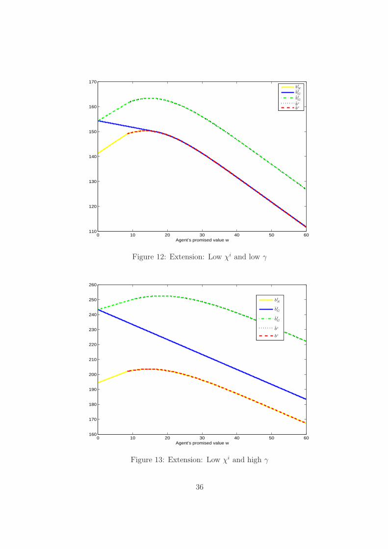
0 10 20 30 40 50 60110

120

130

140

150

160

170

Agent’s promised value w

bℓ

N

bℓ

G

bℓ

G

bc

bc

Figure 12: Extension: Low χi and low γ

0 10 20 30 40 50 60160

170

180

190

200

210

220

230

240

250

260

Agent’s promised value w

bℓ

N

bℓ

G

bℓ

G

bc

bc

Figure 13: Extension: Low χi and high γ

36

0 10 20 30 40 50 6090

95

100

105

110

115

120

125

130

135

Agent’s promised value w

bℓ

N

bℓ

G

bℓ

G

bc

bc

Figure 14: Extension: intermediate χi

37

χi

χn

0 5 10 15 20 25 30 350

5

10

15

20

25

30

35

Incumbent Managerat First Best

New Managerat First Best

New and Incumbent Managers

IncumbentManager No

Growth

New Manager

Figure 15: Who grows the firm ? (big growth opportunity, γ = 0.25)

38

χi

χn

0 5 10 150

5

10

15

Incumbent Managerat First Best

New and Incumbent Managers

Newmanager

Incumbent Manager

No Growth

New Managerat First Best

Figure 16: Who grows the firm ? (small growth opportunity, γ = 0.10)

39