AFRL-SR-AR-TR.06.0287

REPORT DOCUMENTATION PAGE I

The public reporting burden for this collection of information is estimated to average 1 hour por response, including the timeaaltherinR end rnairrtining the date needed, and completing and revieiwlng the collection of information. Send comments regarding tIn.information, including suggestions for reducing the burden, to Department of Defense, Washington Headquarters Services. Directorate for Informasi ..1215 Jefferson Davis Highway, Suite 1204. Arlington. VA 22202-4302. Respondents should be aware that notwithatonding any other provision of law, no person shall I•epenalty for failing to comply with a collection of information if it doe not display a cutrently valid OMB control number.

PLEASE DO NOT RETURN YOUR FORM TO THE ABOVE ADDRESS.1. REPORT DATE (DD-MM-YYYY) 2. REPORT TYPE 3. DATES COVERED (From - To)

05-07-2006 Final August 2005 - June 20064. TITLE AND SUBTITLE 5a. CONTRACT NUMBER

FA9550-05-C-0139Stochastic Resonance in Signal Detection and Human Perception 5b. GRANT NUMBER

Sc. PROGRAM ELEMENT NUMBER

6. AUTHOR(S) 5d. PROJECT NUMBER

Michels, James H. Chen, HaoKay, Steven M. Varshney, Pramod K. 5. TASK NUMBER

5f. WORK UNIT NUMBER

7. PERFORMING ORGANIZATION NAME(S) AND ADDRESS(ES) 8. PERFORMING ORGANIZATION

JHM Technologies, Langmuir Lab, Suite 207, Box 1047, 95 Brown Rd., Ithaca, NY REPORT NUMBER

14850 JHM - 2005 - 06 - 10

Syracuse University - 335 Link Hall, Syracuse University, Syracuse, NY 13244

9. SPONSORING/MONITORING AGENCY NAME(S) AND ADORESS(ES) 10. SPONSOR/MONITOR'S ACRONYM(S)

Air Force Office of Scientific Research875 North Randolph St., Room 3112

Arlington, VA 22203 11. SPONSOR/MONITOR'S REPORTNUMBER(S)

12. DISTRIBUTION/AVAILABILITY STATEMENT

Approved for public release; distribution unlimited

13. SUPPLEMENTARY NOTES

Program Manager: Dr. Willard D. Larkin, AFOSR/NL

14. ABSTRACT

Stochastic Resonance (SR) is a nonlinear phenomenon first reported in terms of a nonlinear dynamic effect. The important questionof what type of noise to be added has until recently evaded a solution. This issue is addressed directly and a fundamental theoreticalframework is developed leading to a determination of the optimal additive SR noise to achieve maximum probability of detectionsubject to the constraint that the probability of false alarm is not increased. Chapters 2 and 3 provide alternative analyticalframework presentations for SR application to detection leading to an optimization solution. Chapter 4 discusses probability of errorreduction with implications for communications theory. Subsequent chapters address applications of the analytical theory tosuboptimal detectors such as nonparametric detectors (Chapter 5), image enhancement (Chapter 6), and distributed sensor fusion(Chapter 7). Chapter 8 provides a novel consideration to an alternative decision statistic transformation methodology to recoveroptimal performance for a suboptimal detector. Finally, Chapter 9 presents recommendations and future considerations.16. SUBJECT TERMS

Stochastic Resonance Noise Enhanced Detection Data Transformation Suboptimal Detector Enhancement DetectionImage Enhancement Image Visualization Human Perception CFAR Probability of Error Reduction Parametric DetectorsSensor Fusion Enhancement16. SECURITY CLASSIFICATION OF: 17. LIMITATION OF 18. NUMBER 19a. NAME OF RESPONSIBLE PERSON

a. REPORT b. ABSTRACT c. THIS PAGE ABSTRACT OF James H. Michels, JHM TechnologiesPAGES

U U U U 19b. TELEPHONE NUMBER (Include area code)

(607) 257- 5740Standard Form 298 (Rev. /98/)Prescribed by ANSI Std. Z39.1B

20060727335

STOCHASTIC RESONANCE IN SIGNAL DETECION

AND HUMAN PERCEPTION

James H. Michels, Hao Chen, Pramod K. Varshney, and Steven M. Kay

FA9550-050C-0139

TABLE OF CONTENTS

LIST OF FIGURES .......................................................................... ivLIST OF TABLES ............................................................................ v

1.0 Introduction ..................................................................................... 1

2.0 Fundamental Detection Framework using Stochastic Resonance (SR) ............... 4

2.1 Introduction to the Fundamental Detection Framework using SR ................ 4

2.2 Problem Formulation ..................................................................... 6

2.3 Optimum SR Noise for Neyman-Pearson Detection ................................. 7A. Determination of SR Detection Improvement .................................. 8B. Determination of the Optimum SR Noise PDF .................................. 9C. Determination of the PDF of Optimum SR Noise ................................ 10

2.4 A Detection Problem Example ........................................................ 10

3.0 An Alternative Derivation for the SR Detection Framework ........................ 14

4.0 Reducing Probability of Decision Error using Stochastic Resonance ............... 22

4.1 Optimal PDF of Additive Noise Sample ............................................. 22

4.2 Derivation of the Optimal PDF for C ................................................. 23

4.3 The Gaussian Mixture Example ...................................................... 24

5.0 Application of Stochastic Resonance (SR) to Nonparametric Detectors ............... 28

5.1 Problem Formulation for Nonparametric Detectors ................................. 28

5.2 Detection Performance for Nonparametric Detectors ............................. 29

A. The Sign Detector ..................................................................... 30

B. The Wilcoxon Detector ............................................................... 32

C. The Dead-Zone Limiter Detector ..................................................... 33

5.3 Experimental Results ..................................................................... 34

5.4 Summary of Results for SR Enhanced Nonparametric Detectors ............... 40

6.0 Application of Stochastic Resonance (SR) to Imagery .................................. 41

6.1 Image Quality Metrics ..................................................................... 41

6.2 Detection Enhancement in Imagery .................................................... 43

7.0 Application of Stochastic Resonance (SR) to Distributed Detection .................. 47

7.1 Stochastic Resonance Problem Statement ............................................. 47

iii

7.2 Decision Fusion and non-ideal Transmission Channels ............................... 47

7.3 Noise Enhance Decision Fusion .......................................................... 51

7.4 Summary of Results for Distributed Detection using SR ........................... 55

8.0 Optimal Decision Processing by the Transformation Method ........................... 56

8.1 Mathematical Description of the Transformation Method ......................... 56

8.2 An Example of the Transformation Method ........................................... 58

9.0 Recommendations and Future Considerations ............................................. 59

9.1 Extensions to the Optimized SR Detection and Estimation Framework ............ 59

9.2 Optimal Decision Processing by the Transformation Method ..................... 62

9.3 Stochastic Resonance in Imagery ........................................................ 62

9.4 Stochastic Resonance in Image Visualization ......................................... 64

9.5 Visual Image Fusion Considerations for Human Perception ....................... 65

9.6 Stochastic Resonance in Distributed Systems ......................................... 68

R eferences ................................................................................................ 69

iv

LIST OF FIGURES

2.1 a.) Plot of U = (f, fo) where fi = Fi(x) and fo = Fo(x), b.) PY versus signal level A, c.) PY

versus co, d.) PY versus it.

2.2 Receiver operating characteristic (ROC), PY versus PFYA.

3.1 Plot of the h(w) function for the example problem.

3.2 Plot of PD(c) versus PFA(C).

4.1 Original PDFs. The left-most PDF modes cross at x = -2.5, which is indicated by the dashedvertical line. The fixed decision regions are indicated by Ri while the optimal ML decisionregions are indicated by R1.

4.2 PDFs after c = 2.5 is added to x. The fixed decision regions are indicated by Ri while theoptimal ML decision regions are indicated by R>.

4.3 Probability of a correct decision versus the value of the constant c to be added to the datasample. The dashed lines are at c = -3.5 and c = 2.5.

5.1 Asymptotic Efficiency of the SR Noise Modified Nonparametric Detectors, (a) based on ys,(b) based on yg.

5.2 Detection performance for the sign detector and the Wilcoxon detector using a finite samplesize N = 5 and signal strength A = 1; a.) based on y, b.) based on yg.

5.3a Probability of detection versus standard deviation r based on y, for the dead-zone limiterdetector with sample size N = 5, signal strength A = 4, and false alarm rate a = 0.1.

5.3b Probability of detection versus standard deviation r based on yg for the dead-zone limiter

detector with sample size N = 5, signal strength A = 4, and false alarm rate a = 0.1.

6.1 Examples of the Visual Information Fidelity (VIF) metric.

6.2 Image enhancement using Gaussian SR white noise, a.) signal image, b.) a signal image plusGaussian mixture noise, c.) sign detector test statistic, d.) sign detector test statistic withGaussian white SR noise, e.) detection using sign detector without SR noise, f.) detectionusing sign detector with Gaussian SR noise.

6.3 Image enhancement using discrete SR noise PDF with nj = -4.0 and n2 = 2.0, a.) test statisticvalues, X = 0.05, b.) test statistic values, ?, = 0.1587, c.) detection results, X = 0.05, d.)detection results, X = 0.1587.

v

6.4 Image visualization using the 'Lena' image, a.) original Lena image, b.) image with a high

threshold applied, c.) Gaussian SR noise, d.) uniform SR noise, e.) optimal discrete SR noise.

7.1 The parallel fusion model.

7.2 A two layer transmission channel model for a distributed detection system.

7.3 Channel model for a signal detection problem in local sensor k.

7.4 Detection performance comparison of different fusion rules and SR noise.

7.5 Deflection Coefficient for different test statistics, A = -0.2.

7.6 Deflection coefficient for SR enhanced 73 decision fusion for different channel SNR.

7.7 ROC curves for various fusion statistics; SNR = 5dB, A = -0.2.

7.8 The equivalent channel crossover errors as a function of A, SNR = 5dB.

8.1 Transforming Function - One of many possibilities.

9.1 Fused images for the speckle noisy 'Lenna' image set with different SNRs. The left columnuses the 'wavelet' method, the center column uses the 'averaging' method, and the rightcolumn uses the 'Laplacian' method. (a),(b), (c): fused results when SNR = 15dB; (d),(e),(f):SNR = 20dB; (g),(h),(i): SNR = 25dB.

vi

LIST OF TABLES

9.1 Performance results for visual image fusion and human visualization.

vii

1.0 Introduction

Stochastic Resonance (SR) is a nonlinear phenomenon first reported and analyzed in [Benzi1981] in terms of a nonlinear dynamic effect. Since then, it was proposed [Benzi 1982] [Nicolis]to explain the observed periodic occurrences of the earth's ice ages using a two state systemdenoting the earth's climate at present and during the ice age. Variations in the absorption andreflectance of incident solar energy due to changing weather conditions constituted the system'noise'. The weak periodic 'signal' consisted of variations of incident solar energy due toperiodic eccentricity in the earth's orbit. Since then, considerable research efforts have assessedthe effect in a wide range of applications including audio systems [Lipshitz], neural networks[Lindner], hyperspectral imaging [Chiang], neuroscience [Kosko], medical imaging [Muller],visual perception [Simonotto], more recently in tactical surveillance [Repperger], as well asapplications cited in the reference section.

The classic SR signature is the signal-to-noise ratio (SNR) gain of certain nonlinearsystems; i.e., the output SNR is significantly higher than the input SNR when an appropriateamount of noise is added. This ratio reflects the gain achieved by the processing procedure.These considerations are treated in references [3] - [17] of [Chen, et. al., 2006b]. Someapproaches have been proposed to tune the SR system by maximizing SNR. It has been shownthat the SNR of a summing network of excitable units is optimum at a certain level of noise[Collins]. Later, for some SR systems, robustness enhancement using non-Gaussian noise wasreported in [Castro, et. al.]. For a fixed type of noise, Mitaim and Kosko [Mitaim, 1998]proposed an adaptive stochastic learning scheme performing a stochastic gradient ascent on theSNR to determine the optimal noise level based on the samples from the process. Rather thanadjusting the input noise level, [Xu, et. al.] proposed a numerical method for realizing SR bytuning system parameters to maximize SNR gain. Although SNR is a very important measure ofsystem performance, SR approaches based on SNR gain have several limitations. Specifically,SNR characterizes only the second order terms of the processes; i.e., the signal and noisevariance. First, the definition of SNR is not uniform and, in fact, varies from one application toanother. Second, to optimize the performance, the complete a priori knowledge of the signal isrequired. Finally, for detection problems where the noise is non-Gaussian, higher order termsmay play a role and optimizing output SNR does not guarantee optimizing probability ofdetection.

SR was also found to enhance the mutual information (MI) between input and outputsignals [Godivier], [Goychuk], [Stocks], [Kosko 2003, 2004], [Mitaim 2004]. Similar to theSNR scenario, for a specified type of SR noise, [Mitaim 2004] showed that almost all noiseprobability density functions produce some SR effect in threshold neurons and a new statisticallyrobust learning law was proposed to find the optimal noise level. [McDonnell] pointed out thatthe capacity of a SR channel cannot exceed the actual capacity at the input. Compared to SNR,MI is more directly correlated with the transferred input signal information.

In signal detection theory, SR also plays a very important role in improving the signaldetectability. In [Asdi] and [Zozor 2002], improvement of detection performance of a weaksinusoid signal is reported. To detect a DC signal in a Gaussian mixture noise background, [Kay2000] showed that under certain conditions, performance of the sign detector can be enhanced by

1

adding some white Gaussian noise. For another suboptimal detector, the locally optimumdetector (LOD), [Zozor 2003] pointed out that detection performance is optimum when the noiseparameters and detection parameters are matched. A study of the stochastic resonancephenomenon in quantizers conducted in [Saha] showed that improved detection performance canbe achieved by a proper choice of the quantizer thresholds. Recently, [Rousseau] pointed outthat the detection performance can be further improved by using an optimal detector on theoutput signal. Despite the progress achieved by the above approaches, the study of the SR effectin signal detection systems is rather limited and does not fully consider the underlying theory. In[Chen 2006b], the underlying mechanism of the stochastic resonance phenomenon was exploredfor a more general two hypotheses detection problem.

The type of detector that lends itself to improved detection via stochastic resonance is onethat nonlinearly processes the data. The eye itself is a nonlinear device and so it is conceivableand has been demonstrated empirically that improved visual detection is possible through thismechanism. The important question of what type of noise to be added has until recently evadeda solution. In Phase I, this issue was addressed directly and a fundamental theoretical conceptwas developed leading to a determination of the optimal additive SR noise to achieve maximumprobability of detection PD subject to the constraint that the probability of false alarm PFA is notincreased.

Clearly, improving visual imagery for human visual perception will depend on the type ofnonlinearity that the eye employs. Ultimately, we know that it is the brain that responds to avisual stimulus causing neurons to fire. Conceivably if we understood the effect of the noisePDF on detectability for the "eye detector", then we could add noise such that the total noisePDF is the most desirable one. This requires a study of a.) the types of noise PDFs that can beobtained via convolution since adding noise random variables causes a convolution of theirPDFs, b.) the most desirable noise PDF from the standpoint of detectability, and c.) how standarddetection theory relates to human visual perception.

We previously pointed out that there are limitations of the signal-to-noise ratio as the mostimportant measure of human detectability. In fact, the SNR measure only characterizes detectionin the Gaussian noise case. For non-Gaussian noise, SNR is only part of the story with, forexample, the intrinsic accuracy providing the remainder in the independent, identicallydistributed (1ID) non-Gaussian detection problem. The intrinsic accuracy is the single sampleFisher information for a DC level in non-Gaussian IID noise [Kay 1998]. Clearly, these twoimportant aspects of design are related and so an overall strategy of noise PDF design isrequired. It was also noted in the Phase I proposal that there are also questions of whether theadditive enhancement noise should be IID from pixel to pixel. It is possible that correlated noisemight be more fruitful. This is an avenue of research that has not been addressed. Furthermore,multivariate PDF design is a difficult problem, but there has been recent progress in this area[Kay 2001], [Tanner 1993], [Ruanaidh 1996], [Gilks 1996]. The above considerations werenoted, but not fully considered in the Phase I effort. In Phase II, we shall return to give morethorough consideration to these issues among others.

The establishment of an analytic framework for algorithmic development utilizing stochasticresonance was a prime objective of the Phase I effort. In order to achieve this goal, it was

2

imperative to assess the relationship of the non-Gaussian nature of the noise processes, the non-linear aspects of the signal processing or suboptimal detection device, as well as thecharacteristics of the sub-threshold signals.

An important consideration here is that the non-Gaussian noise PDF may actually provide apotential for improved detection performance provided that an appropriate detection strategy isemployed. Evidence for this consideration has been noted by [Kay], [Michels] in severalpublications, although not related to stochastic resonance. Several of these analyses involvedpartially correlated non-Gaussian noise processes in addition to additive white Gaussian noise.As noted previously, it is possible that the use of correlated noise may be beneficial in theenhancement of the stochastic resonance effect. Both the application of correlated noise as wellas the assessment of processes already containing such noise is an open area of research whichhas received little attention. It remains as an important research topic for the Phase II effort.

In Chapter 2, a novel fundamental theory addressing the optimization of stochasticresonance in detection theory is outlined. The development of this theory was the primecontribution of Phase I. Specifically, this effort achieved the goal of establishing a fundamentalanalytical framework for the application of stochastic resonance to detection from which anoptimization solution could be obtained. Chapter 3 provides an alternative presentationintroducing the analytical framework. In Chapter 4, a novel consideration is given to thepotential use of an alternative decision statistic transformation methodology to recover optimalperformance for a suboptimal detector. Subsequent subsections address the application of theanalytical detection theory framework to suboptimal detectors such as nonparametric detectors(Chapter 5), image enhancement (Chapter 6), distributed fusion applications (Chapter 7), andprobability of error reduction (Chapter 8) with implications for communications theory. Finally,recommendations and future considerations are presented in Chapter 9.

3

2.0 A Fundamental Detection Framework using Stochastic Resonance

2.1 Introduction to the Fundamental Detection Framework using SR

This chapter summarizes the mathematical framework developed during Phase I to analyzethe stochastic resonance (SR) effect in binary hypothesis testing problems [Chen, et. al., 2006a,b]. Specifically, given an N dimensional data vector x E RN, we decide between two hypothesesH1 and H0,

H0: px(x;Ho) = po(x)HI: p.(x;H) = p1(x) (2.1)

where po(x) and pl(x) are the PDFs of x under H0 and H 1, respectively. The test above can becompletely characterized by a critical function (decision function) 4i where 0 < 4i(x) < 1for all x.For any observation x, this test chooses the hypothesis H1 with probability ý(x). In many cases,4(x) can be implicitly expressed by a test statistic T(x) which is a function of x and a threshold risuch that

H,T(x) >(2.2)

HO

where its corresponding critical function is

I T(x) > q

OT(x) = T(x) = 77 (2.3)0 T(x) < 77

and 0 <a < 1 is a suitable number. The probability of detection PD is now given by

S= f• O(x)Pl(x)dx (2.4)

and the probability of false alarm PFA is given by

= J f,, )O() (2.5)

where the superscripts on PD and PFA in (2.4) and (2.5) indicate that the test in (2.2) isemployed for the data vector x. Although the critical function 4(x) and test statistic T(x) can takeany form, the optimum Neyman-Pearson test involves the likelihood ratio test (LRT) whereTLRT(X) = p1(x)/po(x). Although this test provides optimal PD subject to the constraint that PFA =

cc is fixed, the associated LRT requires complete knowledge of the PDFs p0(x) and pl(x). Inmost practical applications, this knowledge is unavailable and may have to be estimated from thedata. Also, the input data statistics may very with time or may change from one application tothe other. Further, for many detection problems the exact form of the LRT may be toocomplicated to implement. Therefore, suboptimal detectors featuring simplicity and robustness

4

are often preferred [Thomas 1970]. To improve a suboptimal detector detection performance,two approaches are widely used. In the first approach, the detector parameters are varied [Zozor1999, 2002, 2003], [Saha], Galdi]. Alternatively, when the detector itself cannot be altered orthe optimum parameters are difficult to obtain, adjusting the observed data becomes a viableapproach. Thus, in the work reported here, prime consideration was given to applications inwhich such detector parameters could not be changed; i.e., the detector parameters wereconsidered to be fixed in terms of both the test statistic and the threshold. This is often the casefor applications where the signal processing methodology is not under the user's control. In suchcases, we consider the alternative approach of utilizing stochastic resonance.

It is well known that the detection performance can be improved by adding additional noisethat is statistically dependent on the existing noise and/or with PDF that depends in whichhypothesis is true [Kay 2000]. However, adding a dependent noise is not always possiblebecause pertinent prior information is usually not available. Therefore, we constrain the additivenoise to be independent noise. For some suboptimal detectors, as noted in [Kay 2000], detectionperformance can be improved by adding such noise to the data under certain conditions. For agiven type of SR noise, the optimal amount of noise can be determined that maximizes thedetection performance for a given suboptimal detector [Inchiosa]. In an effort to explain thisnoise enhanced phenomenon for some integrate-and-fire neuron models, [Tougaard]demonstrated that the detection performance gain is caused by the nonlinear properties of thespike-generation process itself. However, despite the progress made in the literature, theunderlying mechanism of this Stochastic Resonance phenomenon in detection problems has notbeen fully explored. For example, an interesting problem is the determination of the best 'noise'to be added in order to achieve the best achievable detection performance for the suboptimaldetector. In this case, the detection problem can be stated as: Given that the test is fixed, i.e., thecritical function 4(.), as for example T and q, is fixed, can we improve the detection performanceby adding SR noise? And if so, what is its PDF to maximize PD without increasing PFA?

Here, a theoretical analysis is presented to gain further insight into the SR phenomenon andthe detection performance of the noise modified observations is obtained. Further, the optimumnoise PDF, i.e., not only the noise level but also the noise type is determined. As an illustrativeexample, the optimum noise PDF as well as several suboptimum noise PDFs are derived for thesign detector. We emphasize that compared to some prior work where one or several nonlinearsystems are inserted between the final detector and the original input signal, here, by consideringthe decision function 4 in general and the fact that we may consider the entire system betweenthe input signal and output detection resul as a 'super' detector, the results obtained in this papercan be applied for any detection system with any type of fixed SR preprocessing system. Also,compared to the earlier definitions of SR [Benzi 1981], [Gammaitoni], we further extend theconcept of 'SR' to a pure noise enhanced phenomenon, ie., a phenomenon of some nonlinearsystems in which the system performance is enhanced due to the addition of independent noise atthe input. In the work reported here, the terminologies 'SR' and 'noise enhanced' are usedinterchangeably. However, we point out that the later is actually a generalization of the former.

5

2.2 Problem Formulation

In order to achieve a possible enhancement of detection performance, we add noise to theoriginal data process x and obtain a new data process y given by

y = x + n, (2.6)

where n is either an independent random process with PDF pn(n) or a nonrandom signal. Notethat here we do not have any constraint on n. For example, n can be white noise, colored noise,or even a deterministic signal A, corresponding to pn(n) = 6(n - A). As will be shown later,depending upon the detection problem, an improvement of detection performance may notalways be possible. In that case, the optimal noise is equal to zero. The PDF of y is expressed bythe convolution of the PDFs such that

py (y) = p" Wx * p. Wx = f'p. (x)pn (Y- x)dx. (2.7)

The binary hypothesis testing problem for this new observed data y can be expressed as

fH 0 : py(y;Ho) = JR Po(X)p.(Y- x)dx (2.8)

H1 :py(y;H1)= J, pPl(x)P. (y -x)dx

Since the detector is fixed, i.e., the critical function 4 of y is the same as that for x, theprobability of detection based on the data y is given by,

P1Y = f,, R(y)pY (y;lH)dy

= JRN O(Y) IRN' (x)pn (y - x)dxdy

= R,, p1(x) ( J ,O(y)pn (y - x)dy) dx

= J'R p. (x)C.,1 (x)dx = E1 [Cn,,,(x)] (2.9)

where

CnO (x) J- fRN z(y)pn (y - x)dy (2.10)

Aternatively,

P R= JR Np(x)(JR•I(y)plP(y-x)dy)dx

= JF1,> (x)pn (x)dx = En (F1, (x)) (2.11)

Similarly, we have

6

PYA = R po (x)C.,o (x)dx = Eo [C.,0 (x)] (2.12)

= {Fo, (x)p. (x)dx = E, (F, (x)) (2.13)

wherej (x)j =N,0(y)p,(y-x)dy i= 0, 1, (2.14)

and Fi,ý(x) corresponds to hypothesis Hi, and Ei(.), E,(-) are the expected values based on thedistributions pi(') and pn(.), respectively. Note that Fi(x) has the property that PA = F0, (0) and

P• = Fl,0(0). To simplify notation, we omit the subscript 4 ofF and C and denote them as F1, F0

and Cn, respectively. Further, from (2.14), FI(xo) and Fo(xo) are actually the probability ofdetection and probability of false alarm, respectively, for this detection scheme with input y = x+ x0. For example, Fl(-2) is the PD of this detection scheme with input x - 2. Therefore, it isvery convenient for us to obtain the F, and Fo values by analytic computation of values byanalytic computation if p0, pi and 4 are known. When they are not available, F1 and F0 can beobtained from the data itself by processing it through the detector and recording the detectionperformance. Thus, it is not necessary to have complete knowledge regarding 4(.) and pi(.).From (2.11) and (2.13), we may formalize the optimal SR noise definition as follows.

Consider the two hypothesis detection problem as in (2.1). The PDF of the optimum SRnoise is given by

p, arg max fn ,F1 (x)p. (x)dx (2.15)

where

1) pn(x)_ Ž0,xe RN

2) J1 pn (x)dx = 1

3) J•R F0(x)pn(x)dx < F0(0).

Conditions 1) and 2) are fundamental properties of a PDF function. Condition 3) ensures thatPFY- PxA, i.e., the PFA constraint under the Neyman-Pearson criterion is satisfied. Further, if the

inequality condition in 3) becomes equality, the constant false alarm rate (CFAR) property of theoriginal detector is maintained.

2.3 Optimum SR Noise for Neyman-Pearson Detection

In general, it is difficult to find an exact form of pn(') directly because of condition 3).However, an alternative approach considers the relationship between pn(x) and Fi(x). From(2.14), for a given valuefo of F,, we have x =Fo7(fo), where Fo1 is the inverse ofF 0. When F0

is a one-to-one mapping function, x is a unique vector. Otherwise, Fo'(f 0 ) is a set of x for

which Fo(x) =fo. Therefore, we can express a value or a set of valuesf, ofF1 as

7

fý = F, (x) = Fý (F0)-'(f0)) . (2.16)

Given the noise distribution of p,(.) in the original RN domain, p.,fo (.), the noise distributiom in

thefo domain can also be uniquely determined. Further. the conditions on the optimum noise canbe rewritten in terms offo equivalently as

4) p.,f 0 (fo) > 0

5) Jfp., o (f0 )dfo = 1

6) JfoP.,f(fo)dfo •-PA

and

P = fAnf(fo)dfo, (2.17)

where P,,,f (fo) is the SR noise PDF in thefo domain. Compared to the original conditions 1), 2)

and 3), this equivalent form has some advantages. First, theFroblem complexity is dramaticallyreduced. Rather than searching for an optimal solution in R , an optimal solution is sought in asingle dimensional space. Second, by applying these new conditions, we avoid the direct use ofthe underlying PDFs pj(.) and po(') and replace them withyfi and Jo, respectively. Note that insome cases, it is not easy to find the exact form of fi and fo. However, recall that Fi(xo) andFo(xo) are the probability of detection and false alarm, respectively, of the original system x + x0.In practical applications, we may learn the relationship by Monte Carlo simulation usingimportance sampling. In general compared to p 1 and po, fi and fo are much easier to estimate andonce the optimum p.,o is found, the optimum p.(x) is determined as well by virtue of the

inverse of the function F0 and F1.

Let us now consider the function J(t) such that J(t) = sup(fi: fo = t) is the maximum value off, givenfo. Clearly, J(PA) Ž- Fl(O) = PA. From (2.17), it follows that for any noise p., we have

PNY(P.) = f J(f0)Pf (fo)df•. (2.18)

Therefore, the optimum PY is attained when fi(f) = J(fo) and PY, op, = En(J) .

A. Determination of SR Detection Improvement

A significant contribution of the theoretical framework provided here is the capability todetermine if SR will indeed provide performance improvement in a given problem. Detectionenhancement results using SR results if PD, op > PD. However, it requires complete knowledge of

Fo(-) and F1 (.) as well as significant computation. For a large class of detectors, however,

8

depending on the specific properties of J, we may determine the sufficient conditions forimprovability and non-improvability more readily. These are given in the following theoremsthe proofs of which are contained in [Chen 2006b].

Theorem 1 (Improvability of Detection via SR): If J(PFA) > PD or J"(PA) > 0 when J(t) is

second order continuously differentiable around PFA, then there exists at least one noise process

n with PDF pn(.) that can improve the detection performance.

Theorem 2 (Non-improvability of Detection via SR): If there exists a non-decreasing concavefunction y(fo) where w(PFxA ) = J(PFA ) = F1 (0) and p(t?) _> J(f) for everyfo, then PD < P, for anyindependent noise, i.e., the detection performance cannot be improved by adding noise.

B. Determination of the Optimum SR Noise PDF

Another very significant result of the theoretical framework is the determination of the exactform of poP, subject to the constraint PFYA " PFA. This is contained in Theorem 3 [Chen 2006b].

Theorem 3 (Form of Optimum SR Noise): To maximize PDy under the constraint PYA < PxA, the

optimum noise can be expressed as'

pOp (n) = 25(n-nl)++(1-2)(n-n 2 ) (2.19)

where 0 < k < 1. Specifically, to obtain the maximum achievable performance given the falsealarm constraint, the optimum noise is a randomization of two discrete vectors added withprobability k and (1 - k), respectively. It can also be shown [Chen 2006b] that

pop,f = 25(f fo) + (1 - 4)6(f 0 - f 02) (2.20)

wherefol = Fo(ni) andf02 = Fo(n 2). Alternatively, the optimum SR noise can also be expressed

in terms of C., such that

C1p'"(x) = 2o(x + n,) + (1 - 2)(x + n 2). (2.21)

From (2.20), we have

Dopt = i )±+ 1 -Ak)J(f 0 2 ) (2.22)

and

PFA~opt = 0 l+ (1- )f 0 2 <FA" (2.23)

'This form of optimum noise PDF is not necessarily unique. There may exist other forms of noise PDF that achievethe same detection performance.

9

C. Determination of the PDF of Optimum SR Noise

Depending upon the location of the maxima of J(.), we have the following theorem.

Theorem 4 Let FlM = max(J(t)) = to and to = arg min(J(t) = FlM). It follows that

Case 1: If to PFA ,then P opY = to and PY ---- FmM, i.e., the maximum achievable performance

is obtained when the optimum noise is a DC signal with value no or

P.' (n) = S(n - no) (2.24)

where Fo(no) = to and FI(no) = FlM. Here, the maximum probability of detection is achieved

subject to the probability of false alarm constraint PFY ___ P<XA by adding a constant to the input

with a value that depends upon the decision regions and the probability density functions underthe two hypotheses. However, the threshold must be varied to maintain PFYA _ PxXA.

Case 2: If to>PFA, then PAopY =F0(0)_p, i.e., the inequality of (2.23) becomes equality.

Furthermore,

PA~opt A Mol+(1-)fo2=FA" (2.25)

In this case, the probability of false alarm is maintained without a threshold variation. Thus, the

CFAR property is achieved.

2.4 A Detection Problem Example

The above theoretical methodology was applied to the problem considered by [Kay 2000].Given observation data x[n], n = 1, 2, ... , N, we consider the binary hypothesis testing problemsuch that

H0 :x[n] = w[n] n = 1, 2, ..., N (2-26)

H1 :x[n]=A+w[n] n=1,2,...,N

involving detection of a known dc signal level A > 0 in i.i.d. symmetric Gaussian mixture noisew[n] with PDF

pw(w) = 1y(w;_P, Uo02) + I y(w;, U2) (2.27)2 20

where

2 (W___exr)2Y(W; Pw U6 .)j (2.28)

w2) -22

10

Here, ýI = 3, A = 1 and c0 = 1. The suboptimal sign detector is considered with test statisticI N-1 I I . I N-1

T(x) = +~ ~-+sgn(x[i]) -= lxll (2.29)

1 1

where wuji] = -+ sgn(x[i]) From the second equality in (2.29), we consider this detector as22

essentially the fusion of the decision results from N ii.d. sign detectors. For N = 1, the detectionproblem reduces to a problem with test statistic Ti(x) = x, threshold 71 = 0 (sign detector), and

probability of false alarm pFxA = 0.5. The distribution of x under the H0 and H1 hypotheses can be

expressed as1 1

Po(X) = -y(x;-P,o-2)+ y(x;;P,o-U) (2.30)2 20

and1 2 1

p.(xW =- y(x;-p,+ A, ao ) +-r I(x;,p + A, cU), (2.40)2 20

respectively. The critical function is given by

OW = ýO (2.41)

The problem of determining the optimal SR noise is to find the optimal p,(n) where for the new

observation y = x + n, the probability of detection PY = p(y > 0;H 1) is maximum while for the

probability of false alarm, PY = p(y > 0;H 0) < PFA = -1 It follows [Chen 2006b] that the

resulting optimal SR noise PDF is

p7p,(n) = 28(n-nl) + (1-))8(n-n 2)= 0.30858(n + 3.5) + 0.69156(n - 2.5). (2.42)

It also follows that for the case of optimal SR noise, but now constrained to have a symmetricPDF, p' (x), where p' (x) = pP (-x), we have for the example considered here

Ps"(x W 16(x - p) + I15(x + (2.43S(2.43)2 2

Performance results are shown in Fig. 2.1. First, let us consider Fig. 2.1 a which plots thecurve U = (fi, fo) where fi = Fi(x) and fo = Fo(x). This curve is significant in that it reveals thepotential for detection performance improvement via SR. This is observed by again noting that

for the original data process x, P•xA = FO (0) and PD' = FJ (0). For the problem considered here,PxA = F0(0) = fo = 0.5 and P- = Fý (0) = fi = 0.51 yielding detection probability barely above

PFA. However, as indicated by the curve that upper bounds the convex hull, V, which contains

11

all possible PD and PFA values after SR is added, PY = 0.6915. Thus, the region for potential

performance improvement via SR is the region of the convex hull V that lies above the curve U =(fi, fo). Further, this indicates that if the curve U is a convex function, there is no potential forperformance improvement via SR. Thus, the curve U = (fi,fo) provides an important diagnostictool for the determination of potential performance enhancement.

Fig. 2.1b plots PY versus the signal level A. The lowest curve plots PD with no SR noise.As expected, it increases with increasing signal level. The next three curves, which lie justabove, utilized the optimum PDFs for three symmetric SR noise cases. Ranging from lowest tohighest, the SR noise consisted of white Gaussian, uniform, and the optimal symmetric SR noiseof (2.43), respectively. We observe that for the symmetric SR noise cases, the curves allconverge at A = gt to a common PDY value which lies on the PD curve. Thus, for values ofA > gX,no performance improvement is obtained using symmetric SR noise. However, for small valuesof A, say 0 < A < 0.6, the PY values of the symmetric optimal SR noise case achieves the same

level of performance as those obtained for the case of optimal SR noise with PDF given by(2.42). For A > 0.6, however, the latter optimal noise case achieves superior performance levelscloser to the optimal likelihood ratio test (LRT).

Fig. 2.1c considers the detection performance dependence upon the background noisestandard deviation, o-0. The lowest curve plots P, versus u-.; i.e., the case for which no SR

noise is added. We observe that as a,, increases, PL increases until the noise standard deviation

reaches the level a-1 = 2.942. For low values of a. (high SNR), however, the optimum SR noise

enhanced detector reaches PY & 1, while for the symmetric SR noise enhanced detectors, the

performance is reduced. As a-0 increases, the performance of the SR enhanced detectors

converges to the PD value at cr0 = a"1. This results from the convergence of the bimodal

Gaussian background noise PDF p0(x) to a unimodal PDF as a-0 approaches a-1. At this point,

the decision function O(x) and the LRT test are equivalent for PFA = 0.5. Thus, adding SR noise

will not improve PD and all the detection results converge to PD.

Fig. 2.1d shows each detector's performance with respect to gt for A = l and o-0 = 1. All the

detectors show a decrease in performance as gt increases from zero. However, for t > g-o ; 1.5,the optimum LRT begins to increase with increasing g. To explain this effect, we note that for gt<< •t, the bimodal Gaussian noise is approximately unimodal. However, as these two Gaussianmixture peaks separate, the detectability initially decreases until the peaks are sufficientlyseparated. As gt --> o, the peak separation is sufficient such that the background noise PDF isessentially unimodal for signal level A > 0.

Finally, Fig. 2.2 shows the ROC curve for this problem, but now with N = 30. Again, thesuperior performance of the optimal SR noise enhanced detectors is observed compared with thecases of uniform and Gaussian SR noise. Specifically, the detection performance is much closerto the optimal LRT curve.

12

fY 0.9

0.6 0.~t~.~0.80.16~. o7-

P4 V D .....op

t

-------------opt Sym0.2 - o~- pt Unit

--0- opt WGN. ..... ..... ..No SR

C0 81. 0.4 0,6 f02 0.8 1 0.4 1 2 3 S

a. b.0.0

0.05LRT 0.00

0.9 --- - - --- Opt p

0.85 Opt y0.5. , Opt Unitf L

0.8 -4- Opt WGNm- No SIR N I

0.75 .. . .. .. 1.7 ---------------------.---- - -------------

0.70.65N

.5

- p

0.65

0.55 -. "'~~'~ 0.00.6~. .

0.67:

0 0.5 1 15 2 2.5 3 3.5 4 0 1 2 3 4 5 86 7 8 9 I

C. d.Fig. 2.1 a.) Plot of U =(fl,fo) wherefi =F 1(x) andfo =Fo(x), b.) PYversus signal level A, c.) PDY

versus ca0 , d.) PDY versus i..

0.7

0.6

005

0.3' Opt Unit

'---Opt WON

0.. .2..........................No SR

0 0.1 0.2 0.3 0.4 0.5 0.6 0.7 0.8 0.0 1

P FA

Fig. 2.2 Receiver operating characteristic (ROC), PDY versus PY

13

3.0 An Alternative Derivation for the SR Detection Framework

The following derivation [Kay, 2005] addresses the problem of deciding between twohypotheses based on a single sample. The sample may be a single data sample or a test statistic.The scalar test statistic is x, which under H0 has PDF p0(x) and under H1, pl(x). It is assumedthat we decide H1 ifx > 0. Now consider the same detector but replace x by y = x + c, where c isa random variable that is independent ofx. Then, we decide H1 if y = x + c > 0. The PDF of c ispc(c) and it is this PDF that is of interest. We allow the use of impulses in the PDF so that c maybe either continuous, discrete or mixed variable. For this detector, the probability of false alarmand probability of detection are

PFA fpr'(y)dy (3.1)0

PD = fpr (y)dy (3.2)0

where the PDFs of y are

po (y) = Po(Y-c)pc(c)dc

y= p, (y -c)p,(c)dc

which follows from the usual result for the sum of two independent random variables. Explicitlythen

PFA = f[op (y-c)pc(c)dcdy

= po (y - c)dyp (c)dc-~0

= JPFA(C)PC(c)dc

where PFA(c) = Jpo (y - c)dy denotes the conditional probability of false alarm. It is the0

probability of false alarm conditional on observing C = c. Note that the unconditionalprobability of false alarm PFA is just Ec[PFA(C)], where Ec denotes expectation with respect tothe PDF pc(c). Similarly, we have

PD f PD (c)pc (c)dc = Ec[PD(C)]

14

where

PD(C) = fp. (y - c)dy.0

It is interesting to note that PD(C) is just the probability of detection for the original detectorbut with the threshold, originally given by zero, replaced by -c. This is because we decide H1 ify = x + c > 0 or equivalently if x > -c. The threshold, however, is a random variable and hencethe overall detector performance is given by the expected value Of PD(C).

Our problem has now reduced to the following. Choose pc(c) so that Ec[PD(C)] ismaximized subject to the constraint that Ec[PFA(C)] = ½/. (We assume continuity of the originalROC so that the false alarm constraint is an equality). To proceed further it is useful to simplifyPFA(c) and PD(C). Consider

PFA(c) = fpo (y - c)dy0

=fpo(t)dt (lett=y-c).-C

Now note that in this form it is clear that PFA(C) is just the complementary distributionfunction or right-tail-probability. Also, as such, it is obvious that as c increases (-c decreases),that PFA(c) also increases. Thus, PFA(C) is monotonically increasing with c. It is well known thatif a function is monotonically increasing, then the inverse function exists and it too ismonotonically increasing; for example, g(x) = exp(x). Thus, we will use a variable change byletting u = PFA(C), where if -oc < c < oc, we must have 0 _< u < 1. Also the inverse function is

denoted as c = PFA (u). Hence, we now have the new random variable U = PFA(C) and therefore

PFA = Ec[PFA(C)] = Eu[U] = fup, (u)du0

and similarly(UM = EcPoC) M' (u"p "ud

PD = Ec[PD(C)= Eu[PD(PFA (U))] =PD (PA (u))Pu (u)du.0

Recall that we desire PFA - 1/2. Thus, the equivalent optimization problem is to maximize

J(pu) = JPD (PFA (U))Pu (u)du (3.3)0

subject to the constraint that

15

I

fup, (u)du =A½.0

However, it is more convenient to write the constraint as

k(u-l12)pu(u)du =O=Eu[U-Y2]0

and to define a new random variable W = U - V2 so that the constraint becomes Ew[W] = 0.Then, J(pu) becomes from (3.3)

J(pu) = Eu[PD( PF (U))] = Ew[PD(P' (W + 1 / 2))] = J(pw)

where explicitly

1/2J(pw) J PD(P(W+I/2))p,(w)dw

-1/2

1/2

= Jg(w)pw(w)dw-1/2

andg(w) = P. A(w1/2)

Summarizing, we wish to maximize over pw(w) the functional

1/2

f g(w)pw (w)dw-1/2

subject to the constraint that Ew[W] = 0. Note that the random variable W - PFA(C) V- 2 takes onvalues in the interval [-1/2, 1/2]. We can further simplify the problem by maximizing thefunctional

1/2f (g(w) -(w+l1 /2))pw (w)dw

-1/2

since f/2 (w + I / 2))pw (w)dw = ½ due to the Ew[W] 0 constraint. Letting

h(w) = g(w) - (w + 1 2)

which is explicitly

h(w) = PD (PF (W2( ) (3.4)

16

we finally seek to maximize

1/2

f h(w)pw(w)dw-1/2

subject to the constraint that Ew[W] = 0. Note that the function h(w) takes on nonnegativevalues if PD(c) > PFA(C) (the ROC for a variable threshold of the detector that decides H1 ifx > -cis above the 450 line). This is because

h(w) = PD(PF,(w+1/2)) - (w + ½) = PD (PF(U)) - U = PD(C) - PFA(C) Ž0.

Also, at the end points of the [-1/2, ½/2] interval in w we have

h(-1/2) = PD(PFA(O)) = PD(+oo) = 0

h(1/2) = PD(PýA'(1)) - I = P,(--o) - 1 = 0.

A typical plot of h(w) is shown in Fig. 3.1. This example will be used later.

0.2 I I I

0.15 - - ', ,

0 .1 --F --

0.05- -- - -- --

0 -- -- - L.i

-0.05 F F F FI

-0.5 -0.4 -0.3 -0.2 -0.1 0 0.1 0.2 0.3 0.4 0.5

wFig. 3.1 Plot of the h(w) function for the example problem.

In essence, we have modified the function F, versus F0 in Section 2.0 so that it is plotted asthe difference between the function and the 450 line. (See also Fig. 2.l1a for F, versus Fo). Also,it has been shifted to be defined over the symmetric interval [-1/2, 1/2]. This has the advantageof simplifying extensions of the results given here. In addition, the maxima, which will berequired later, are easily found numerically using efficient routines such as a golden search.

The problem now is to maximize the functional

17

1/2

J(pw) = f h(w)pw(w)dw (3.5)-1/2

subject to the constraint that Ew[W] = 0. The function h(w) is nonnegative over the interval [-1/2,1/2]. To simplify the discussion we will assume that h(w) has a unique maximum over theinterval (0,1/2), and a unique maximum over the interval [-1/2, 0]. The maximum is assumed notto occur at w = 0. Also, it is assumed that the maximum values are equal. These assumptionsare satisfied for the example given in [Kay, 2000]. (More rigorous and general results can beobtained using standard theorems in analysis such as 'continuous functions on compact sets',etc.). Once the optimal Pw is found, the PDF for C or Pc can be found by transforming back to Cusing the relationship W = PFA(C) - V2 and the standard results in transformation of randomvariables. Note that if the maximum of h(w) over the interval [-1/2, 1/2] were to occur at w = 0,then the constraint Ew[W] = 0 would be satisfied for pw(w) = 8(w) and J(pw) would also bemaximized. Thus, the solution would be to choose c = PA(w+1/2) = P•(1/2) = 0 and noimprovement in performance would be possible.

Continuing, we let w- be the value that maximizes h(w) for w < 0 and w+ be the value thatmaximizes h(w) for w > 0 (w = 0 is excluded), and assume that h(w.) = h(w+). Let the set Adenote the remaining portion of the interval [-1/2, 1/2] so that { w-, w+} u A [-1/2, 1/2] and{w., w+} r) A = 0. Next, represent pw(w) as

pw(w) =a( w.)8(w - w) + C( w+)6(w - w+) + pw(w)IA(w) (3.6)

where 8 denotes the Dirac delta function and IA(w) = 1 for w E A and is zero otherwise (theindicator function). Actually, any PDF may be decomposed this way subject to the conditionthat

a(w.) + ±a(w+) + JA P, (w)dw = 1.

Using this in (3.5) produces

J(pw) = h(w_)cL( w-) + h(w+)ot( w+) + f h(w)p,(w)dw. (3.7)

In order to satisfy the constraint, we must have that pw(w) has mass for w > 0 and w < 0 (orthe probability of W being negative is nonzero and the probability of W being positive is alsononzero). Otherwise, we could not have Ew[W] = 0. The constraints on pw(w) form the twolinear equations

cL( w.) + a( w+) + JA pw (w)dw = 1

(w.) w_ + a(w+) w++ J wpw )dw 0.

18

In matrix form the constraints are

Aa = bor

['~ 1[a~?] [I- fl Pw(w~dw] (3.8)

where A, a and b are defined implicitly. With h = [h(w.) h(w+)]T, we have from (3.7)

J(pw) = hTa + fI h(w)p, (w)dw

= hTX-lb + fJh(w)pw(w)dw

[h(w-) h(w+)] f h(w)p+(w)dw

W+ w-ww, wd

- [w+h(Twý)-w(w+) h(w+) - h(w-) I[ -, I Pw(w)dw + fh(w)p,(w)dw.

Lw +-wUL IL- L wp,(w)dw A

We point out that the two terms in the first bracket can be expressed as

w+h(w_)-w h(w+) = h(w+)w+-w_

W+ -

and

h(w+)- h(w) 0.

W+ --

Recalling that h(w.) = h(w+) and recognizing that h(w) < h(w+) for all w • A, we have that

J(pw) h(w+) + IA (h(w) - h(w+))pw (w)dw

<h(w+).

Clearly, the upper bound is attained when pw(w) = 0 for all w c A. This results in the solutionfrom (3.6) of

pw(w) - W+ 9(w - W)- + _ 15(w - w+) (3.9)w+ -w_ w_ -w+

where we have solved for cc(w_) and a(w+) by using (3.8) with the right-hand-side vector being [10]. Since W can only take on values w- and w+, it follows that the only values C can take on are

19

c- P-(w +1/2)

c+ PA(w+ +1/2). (3.10)

The optimal PDF for C is therefore

pc(c) w+ 5(c-c-)-+ - 5(c-c,) (3.11)w+-w_ w_-wW+ - V - W+

where c- and c+ are given by (3.10) and w. and w+ are the values that maximize thePD (PF' (w + 1/ 2)) - (w + 1/ 2) for -1/2:< w < 0 and 0 < w _ /2, respectively.

We again consider the example [Kay 2000] of Section 2.0 and assume only one sample asdescribed above. The PDFs are given by

PO x) exp )+ exp(2 1 --- 2 12-;-2

pI(X) = po(x- 1).

Since for a fixed c we decide H1 ifx > -c, we have

1 1PFA(C)= -Q(-c-3)+- Q(-c + 3)

2 2

PD(c)= -Q(-c - 4) + -Q(-c + 2)2 2

where Q(x) is the right-tail probability for a standard normal random variable. This is plotted inFig. 3.2. The function h(w) is given by (3.4) as

h(w) = PD (PFA- (w+1/2))-(w+1/2)

and can be evaluated over [-1/2, 1/2] as in Fig. 3.1. A numerical search finds the maxima ofh(w), which when converted to c yields c- = -3.507 and c+ = 2.493. The other values become

W+ 0.694 and w 0.306w+ -w w -w+

so that the optimal PDF is

pc(c) = 0.3065(c + 3.507) + 0.694&(c - 2.493)

in agreement with the results obtained in Section 2.0.

20

0.5 - - - -

0.8 - - - -

0 . -C I - - - I

0.7 -. L - -.-

Fig. 3. PltO dI vru F()

I I I II 21

4.0 Reducing Probability of Decision Error using Stochastic Resonance

In this chapter, we address the problem of reducing the probability of decision error of anexisting binary receiver that is suboptimal using the ideas of stochastic resonance. The optimalprobability density function of the random variable that should be added to the input is found tobe a Dirac delta function, and hence the optimal random variable is a constant. The constant tobe added depends upon the decision regions and the probability density functions under the twohypotheses, and is illustrated with an example. Also, an approximate procedure for the constantdetermination is derived for the mean-shifted binary hypothesis testing problem.

Here, we consider the problem of deciding between two hypotheses Ho and H1 that canoccur with a priori probabilities P[Ho] = no and P[H1] = 7r1 = I = nto, respectively. Our criterionfor performance will be probability of error Pe, although the derivation is easily modified tominimize the Bayes' risk by assigning costs associated with each decision [Kay 1998]. It isassumed that the decision regions have already been specified, that they are not optimal in termsof minimizing Pe, and that a single data sample x is used to make a decision. The alreadyspecified decision regions may be arbitrary and hence our solution encompasses such regions asif one would decide H1 if x > a or jxi < a as examples. The single sample is usually a teststatistic, i.e., a function of a set of observations, which is a common procedure in decisionmaking. To improve the performance, "noisy sample" c is added to form y = x + c prior todecision making. We allow c to be a random variable and determine the PDF of c that will yieldthe minimum Pe. It is proven next that the optimal PDF is a Dirac delta function, which leads tothe conclusion that the optimal random variable to be added is a degenerate one, i.e., a constant.

4.1 Optimal PDF of Additive Noise Sample

To write the probability of error for the original problem, we define the decision rule (alsocalled the test function or critical region indicator function) as

W =decide H°

Ix =decide H,

Then, we have

P, = P[decide H, I Ho ]P[Ho] + P[decide Ho I H, ]P[H1 ]

= P[5(x) = I I Ho];r0 + P[q(x) = 01H,];r,

- 0 f 0(x)px (x)dx±,;1 L(1-I-(x))px (x)dx

where px (x) and pX (x) are the probability density functions (PDFs) under H0 and H1,

respectively. This can be written as

P, = ;'l + L O(x) [gopx (x)- 7'•px (x)] dx

22

Now assume that we modify x by adding c so that the test stistic becomes y = x + c, where c is arandom variable independent of x, and whose PDF is pc(c). Since the identical decision rule is tobe used, we have

P = =r; + (x)[;roPo(y)-;r~pr(y)]dy.

But

p0 (y) = po' (y - c)pc (c)dc

pr (y) = f• p(y-c)pc(c)dc.

We have then that

Pe= 7r1 + E• O(x)[)r, E px (y-c)pc(c)dc-;rl f•ipx (y-c)Pc(c)dc•_y

= ),r + f[f i(y) (iropx(y - c) - grpjx'(y -c))dy]Pc (c)dc

I ,:+ Ec 0Y(Y) (0 Pox (Y-C)-rP x (Y -c))dY]

where Ec denotes expected value with respect to pc(c). Hence, we wish to choose pc(c) so thatthe slightly more convenient form

J(Pc) = Ec [ 0 o (y) ((0 p0 x (y - c) - 7rlpx (y - c))dy] (4.1)

is maximized. This is done in the next section. We will see that the random variable C may bechosen as a constant and therefore we need only maximize the expression within the brackets of

(4.1) over a constant c. But this is equivalent to shifting 4(u), the decision region function by -C.Hence, the solution effectively shifts the decision region by a constant. This suggests thatanother means for improving performance is to transform the decision region using a nonlineartransformation (instead of a simple shift). It can be done by transforming the data sample x usinga nonlinear transformation g as g(x). This is addressed in Chapter 8 and will be consideredfurther in Phase II.

4.2 Derivation of Optimal PDF for C

It is well known that Ec[g(C)] is maximized by placing all the probability mass at the value

c for which g(c) is maximized. We assume that the function g(c) has at least one point at whicha maximum is attained. Calling this point co the optimal PDF is then pc(c) = 6(c - co), where

eo = argc max g(c)

or

23

co = arg, max L 0(y) (r 0p (y - c) - jrpx (y - c))dy.

A slightly more convenient form for g(c) is obtained by letting u = y - c so that

g(c)= fe (u+c)(;rp((u)- Topox(u))du (4.2)

which is recognized as a correlation between 4(u) and ;rjpX(u)-;ropx(u). In summary, we

should add the constant c to x, where c is the value that maximizes the correlation given in (2).Since the decision function 4(x) in (4.2) is completely general, the optimal solution is valid for agiven binary decision rule with any decision region. For example, if the original decision rulewere to decide H1 ifx > a, then we would use 4(u) = 1 for u > a, and zero otherwise in (4.2). If itwere to decide H1 if lxi < a, then we would use 4(u) = 1 for lul < a, and zero otherwise in (4.2).(Note that if 4(u) = 1 for ;rlpx (u) - irpx (u) > 0 and zero otherwise, then g(c) is maximized for

c = 0. This is because in this case the decision rule 4(u) is optimal.) In the next section we solvethis for a given example.

4.3 The Gaussian Mixture Example

We now consider the problem described in [Kay 2000]. but instead choose the probability oferror criterion. The problem is to decide between px (x) and px (x) = px (x - A), where A > 0

is a DC level that is known and the noise PDF is the Gaussian or normal mixture

pI (x) = p, U2) + N(x,-p, U2) (4.3)

where

N~;,, ')exp I (X -p) 2 i, 2 r-ý2 1-2Cr

2 J

The original decision rule is to choose H1 ifx > 0 so that 4(x) = us(x), where u,(x) is the unit stepfunction. Additionally, we assume equal a priori probabilities so that TEO = 1 = V2. As a result,we have from (4.2) that

-j) f u, (u +c) (pX(u) - po(u))du

=f(px(u)-po(u))du

= -[(1 - Fl (-c)) - (I - F0 (-c))]

= '[Fo(-c)-Fl(-c)]

where F, is the cumulative distribution function of x under the hypothesis H-. For our problem,we have that pX (x) = px (x - A) and so F, (x) = F0 (x- A). Thus,

24

g(c) = -[F. (-c) - Fo (-c - A)]

and differentiating and setting equal to zero produces

pox (-c) = pox (-c - A)

or equivalently since px (x) is even, we have the general requirement

Pox (c) = pox (c + A). (4.4)

Using (4.4) in (4.3) produces

O(c;,p,0c') + ±(;(;-pu,a') = 0(c + A; p, o-') + O(c + A;-u,0C2 )

which upon simplification yields the equation

exp(c / Co2 ) + exp(-uc / c-2 ) = exp [(-c(A - p)/C2) -A A/(2/()2 + ,uA/2C2]

+ exp[(-c(A+p)/I&)-A2/(2C2))-,uA/C.2].

For ýt = 3, a 2 = 1, and A = 1, we have

exp(3c) + exp(-3c) = exp(2c + 5 / 2) + exp(-4c - 7 / 2).

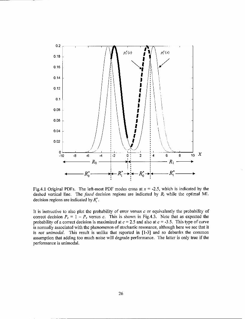
The exact value of c found through a numerical search is c = 2.50, which could also be found byignoring the terms exp(-3c) and exp(-4c - 7/2) since these are nearly zero for this value of c.Another solution is found by ignoring the other set of terms to yield c = -3.5. Note that either ofthese choices causes the PDFs of x + c under H0 and H1 to cross at the origin (see Figs. 4.1 and4.2). If we did not have the right-most Gaussian mode, then the choice of c = 2.5 would result ina maximum likelihood (ML) receiver, which is optimum [Kay 1998]. This is because amaximum likelihood receiver chooses the hypothesis whose PDF value is larger. In our case, thefixed decision regions are R1 = {x: x > 0} for H, and RO = {x: x < 0} for H0 as shown in Fig.4. 1.These decision regions are not optimal. The optimal ML decision regions are indicated inFig.4.1 as Ro and R,. Therefore, the region in x for which Ro # R1, which corresponds to the

dark PDF lines, will result in incorrect decisions. By the addition of c, however, the extent ofthis incorrect decision region is reduced, as indicated in Fig.4.2.

25

0.2 .

0.18p(x) ji pj (x)

0.16 I\

0.14 /

0.12

0.1

0.08

0.06 ,

0.04

0.02 1

0 __

-10 -8 -6 -4 :-2 0 2 4 6 8 10 XSI i

-Ro R, "RSI iI

- R* R4 R R R0 0

Fig.4.1 Original PDFs. The left-most PDF modes cross at x = -2.5, which is indicated by thedashed vertical line. The fixed decision regions are indicated by R; while the optimal MLdecision regions are indicated by R>*.

It is instructive to also plot the probability of error versus c or equivalently the probability ofcorrect decision P, = 1 - Pe versus c. This is shown in Fig.4.3. Note that as expected theprobability of a correct decision is maximized at c = 2.5 and also at c = -3.5. This type of curveis normally associated with the phenomenon of stochastic resonance, although here we see that itis not unimodal. This result is unlike that reported in [1-3] and so debunks the commonassumption that adding too much noise will degrade performance. The latter is only true if theperformance is unimodal.

26

0.2

0.18 / p.(x)

0.16/

0.14 ,

0.12 / U

0.1

0.08

0.06 /0.04;

0.02

-10 -8 -6 -4 -2 0 2 '4 6 8 10 X4Ro '0: RI 1

', 'R,' R,R•

Fig.4.2 PDFs after c = 2.5 is added to x. Thefixed decision regions are indicated by Ri while theoptimal ML decision regions are indicated by R,.

0.6

0.59

0.58

0.57

0.56

Q 0.55

0.54

0.53-

0.52

0.51

0.5-10 -8 -6 -4 -2 0 2 4 6 8 10

c Value

Figure 4.3 Probability of a correct decision versus the value of the constant c to be added to thedata sample. The dashed lines are at c = -3.5 and c = 2.5.

27

5.0 Application of Stochastic Resonance to Nonparametric Detectors

Here we consider detection performance of two additional nonparametric detectors whichexhibit improvement via additive SR noise; namely, the Wilcoxon and the dead-zone limiterdetectors. In addition to the sign detector, these detectors were considered in [Chen, et. al.,2006c]. The asymptotic efficiency (AE) as well as finite sample detection performance of theseSR modified detectors was reported. For large sample sizes, the AE of the Wilcoxon and thedead-zone limiter [Kassam 1976] detectors was shown not to improve by the addition of SRnoise. However, for finite sample sizes, both of these detectors show improvement in thepresence of additive SR noise.

Nonparametric detectors have received considerable attention in signal detection problems[Kassam 1980]. An important feature of such detectors is their guaranteed level and reasonablepower for large classes of input distributions. However, in most cases, a nonparametric detectoris less efficient than the optimal detector. Therefore, an important consideration is the potentialimprovement of their performance while maintaining their false alarm rate (CFAR) property.Here, we explore the potential detection performance improvement of several nonparametricdetectors by adding SR noise to the observed data.

5.1 Problem Formulation for Nonparametric Detectors

Let us consider a detection problem based on the observed data vector x = [xl, x2, ... , XN]with probability density function p(x), where the xi, i = 1, 2, ... , N are independent identicallydistributed (i.i.d.) scalar random variables. We decide between hypotheses HI and Ho given by

Ho :p(x) = H f (xi)1' (5.1)

H," p(x) = f(xi - A)

where the pdff,(.) of the scalar random variable xi is symmetric, i.e., fx(x) = fx(-x) and A > 0.Therefore, this test is essentially the detection of a constant positive DC signal A in additivenoise. with a symmetric pdf.

Following the SR approach, detection performance enhancement is achieved by addingnoise n = [nl, n2, ... , nN] to the original data process x to obtain a new vector y = x + n, where niare i.i.d. scalar random variables with pdffn(n). The constant false alarm rate (CFAR) propertyis maintained by retaining the symmetric pdf property of x. Therefore, we restrict fn(n) to besymmetric, i.e.,fn(n) =fn(-n). Givenfi(x) andfn(n), the pdf of yi under the H0 hypothesis can beexpressed by the convolutions of the pdfs such that

fy (yi) =fx (xi) * fn (ni)

= .f(xi)f(yi -ni)dx1

28

= Lofx(yi -ni)f 1 (xi)dxi. (5.2)

It can be shown that fy(y) =fy(-y), i.e., fy(y) is a symmetric function. Therefore, P(y > 0IHo)1/2., and the CFAR property of the nonparametric detectors is maintained.

The binary hypotheses testing problem for this new observed data y can be expressed as:

Ho :P(Y) = F1- fy (Yi)

NHi" P(Y) = -If, (Yi -- A)

The cumulative distribution function (cdf) of yi is given by

Fy(yi) = L ftfx(xi)f.(yi -xi)dxidyi

= L ff(x( i)fn(Yi -xi)dxidyi

= f. (Xi)Fn (yi- xi)dxi = L fn(xi)Fx (yj -xi)dx. (5.4)

5.2 SR Detection Performance for Nonparametric Detectors

Detection performance for the three detectors is now considered using stochastic resonancefor the problem involving a known DC level in Gaussian mixture noise with mean ýt = 3 andmodal variance a2 = 1. In the asymptotic case where signal strength vanishes and sample sizesapproach infinity, the performance is evaluated in terms of the asymptotic relative efficiency(ARE) between the original detector and the SR noise modified detector. Further, the ARE canoften be expressed as the ratio of their asymptotic efficiencies given by

dE[T(xN)] IA=oE = lim dA(5.5)

N-*o NVarA=o[T(xN)]

where T(.) is the test statistic. Similarly, for the finite sample case, we compare the relativeperformances by the deflection measure [Picinbono 1995] which is defined as

D(T) = [E(T I H) -E(T I H1)]2 (5.6)var(T I H0)

for the sign and Wilcoxon detectors. For the dead-zone limiter detector, we illustrate theperformance by several examples.

29

A. The Sign Detector

For the sign detector, we have a test statistic and decision rule as follows

H,T, =I)- sgn(xi)><r7 (5.7)

H,

where sgn(x) is the sign of x, given by

sgn(x) = x>0 (5.8)

x<O

Let p x= P(sgn(x) = 11H-), i = 0, 1. From, (5.1), we have Pox = f(x)dx = 0.5 and

Px f•f(x - A)dx

2 (a.f(x)dx)Fx(A) = Q +

Furthermore, the test statistic Ts is binomially distributed with parameter Pi under Hi, i = 0, 1.Since, Pox= 0.5 is fixed, therefore when px> 0.5, the detection performance of the sign detector

is monotonically determined by Px, i.e., the higher the value ofPJx, the better the detection

performance of (5.7). It can also be shown that the expected value of T, under Hi is expressed asE(TslHi) = NPJx, i = 0, 1 and the variance of T under H0 is var(TIHo) = N/4. The deflection

measure of the sign detector Ds is given as

Dx = 4N(PJx - p0o)2 = 4N(PI _ 0.5)2. (5.10)

Similarly, for y, we have PIy= 0.5 = Pox andDy =4N(Ply- 0.5)2. However, due to the

additive SR noise n, PIy is changed such that

ply= fA f(y)dy

=-F f f, (Y -X) fn(x)dx dy

- f fn(W f f,(y)dydx

- f f(x)F,(A+x)dx

- f2f,(x)[Fx(A+x)+ F(A-x)]dx

30

- ff(x)G(x)dx (5.11)

The right hand side of (5.11) is obtained by applying the symmetry property off,(x) and lettingG(x (A+x)+F(A-x) From (9), Px = G(O). Let GM = max(G(x)) and xg be the

2

minimum non-negative x such that G(x0) = GM. Since f f,, (x)dx = 1, we have PY •_ GM. The

equality can be obtained be selecting an optimum SR noise pdf f,, such that

fo (x) = 1-(x -x9) + 1S(x + xg). (5.12)

2 2

Therefore, when GM > G(O), the detection performance of the sign detector can be improved byadding SR noise. Correspondingly, its deflection measure is such that Dyo > Dx. Note that G(x)

can be expressed as

G(x) + Fx(A+x) + Fx(A - x)2

_ FJ(A+x)+ 1 - Fx(-A+x)

21 1 IA+x ( . 3= E+ x ff(t)dt. (5.13)

Therefore, for the asymptotic case where N -> oo and A -+ 0, it follows that G(x) ;t V+ Afx(x) sothat G(0) ;t V+ Afx(0). As a result, the asymptotic detection performance can be improved iffx(O) # max(fx(x)). The same conclusion can also be obtained by evaluating the asymptoticefficiency and the ARE between the original detector and the SR noise enhanced detector. Forthe sign detector, its asymptotic efficiency is given by

EX = 4f2(0) (5.14)

and similarly

EY = 4 f7(0) = 4[ I x X~]2. (5.15)

Again since f f,. (x)dx = 1, the optimum SR pdf for this case is

f°W(x) 1s(x-Xo)+ 1s(x+Xo) (5.16)2 2

31

where fx (xo) = max(fx (x)). In general, we have the ARE between the noise modified detectors

and the original detectors Ey,x given by

EYx = fY2(0) (5.17)

B. The Wilcoxon Detector

The Wicoxon detector test statistic is expressed as

N i=j H,

Tw - sgn(xi + xj)<7. (5.18)j=l i=1 H0

In the asymptotic case, the asymptotic efficiency of the original Wilcoxon detector E1 is given

by Ex = 12 [ff7(x)dx . Let Hx(co) = ffx(x)exp(-joix)dx be the Fourier transform of

f.(.). Sincefx(x) _ 0 is a symmetric real function, Hx(co) = ffx(x)cos(ox)dx is also a real

function. From Parseval's theorem, we have

12[ ff�f2(X)dx] 6 '[ H[ H (c)d ]2 (5.19)Ex = 12 X X]

(5.19)

Similarly, the asymptotic efficiency of the SR noise modified detector E1 can be expressed as

Ey = 12 [f (y)dy] = [H>o)dco. (5.20a)

From (5.2), we have HY(co) = Hx(co) Hn(o), so that

Ewy = 6 HY2(o)H,2 (co)do] (5.20b)

and the ARE between the noise modified detectors and the original detectors is given by

EY,x = (L ) (5.21)

Note that

32

H,,(co)l = _ f, (x) exp(-jaox)dx

f'f(x)cos~cox)dxI

< f ,f(x) I cos(cox)I Id

< Ef,(x)dx = 1.

Therefore, we have Hi(ow) <5 H,(to) and furthermore, E, < Ex,. In other words, in the

asymptotic limit where N --> oo and A -- 0, the Wilcoxon detector performance cannot beimproved by adding independent SR noise. However, the detection performance may still beimproved in the finite sample case.

C. The Dead-Zone Limiter Detector

The dead-zone limiter detector [Kassam 1976] employes the dead-zone limiter characteristic1, to operate on the data where lc(') is given by

lC(x){ = -c < x • c (5.22)

x<c

where c is a prescribed positive number. Let Ncp be the number of samples which satisfy xi > cand N, be the number of samples which satisfy Ixil > c. In order to obtain a false alarm rate, a,the dead-zone limiter detector selects the H1 hypothesis with probability one when Ncp > g,(N,)and with probability P3a(Nc) when Ncp = ga(Nc). Both ga(N.) and P3a(Nc) are suitable functionssuch that the false alarm rate is fixed at a. For the dead-zone limiter detector with parameter c,assuming Fx(c) < 1 andfx(c) is continuous at c, we have its asymptotic efficiency Exz given by

ED7 = 2 fX(c) (5.23a)1-Fx(c)"

Thus, for the SR noise modified detector, its asymptotic efficiency is expressed as

EY = 2 f 2 (c) (5.23b)1Z -FY(c)"

The ARE between the SR noise modified dead-zone limiter detector and the original dead-zonelimiter detector is given by

33

- fy 2(c)/(1 - Fy (c)) (5.24)EDZ~ fx2 (c) /(I - Fx (c))

Using (5.2) in (5.23b), we have

E~z -2 f•2 (c)

S 1-F(C)

_ 2( Jf(c-x)fo(x)dx)21 - F•F (c-x)f(x)dx

2(- (F (c - x)f (x)dx

= 2(ff2(c -x)f ,(x)dx) (5.25)

2fZ- ,(c -x)) ff((c)

Let2f (c - x) . Therefore, when c is selected to maximize Exz i.e., K - - ,(cS a- Fx(c - x) i - Fx(c)

we have E~z < Exz. Thus, the asymptotic efficiency of the tuned dead-zone limiter detector

with optimal parameter c cannot be improved by adding SR noise. However, (5.25) does notrule out the possible SR effect when c is not optimum. Furthermore, similar to the Wicoxondetector, for the finite sample and vanishing signal case, the detection performance of the dead-zone limiter detector may still be improved by adding suitable SR noise.

5.3 Experimental Results

Here we consider the detection of a known DC signal in symmetric Gaussian mixture noise;i.e.,

fx(X) =Y(x;-P, o-) + Y(x; P, Co)where

y ( x ; ,p , o-C 2 ) - • e x p 2 o -)

2is the PDF of a Gaussian random variable with mean g and variance a . We consider two typesof SR noise. These include the symmetric two-peak random noise with two random values

fi(x) = 0.55(x - r) + 0.58(x + t) Symmetric two-peak SR noise

and white Gaussian SR noise

fg(x) = 'Y(x;O,t 2). Gaussian SR noise

34

The noise modified data processes are denoted as ys and yg, respectively. In this example, we setGo = 1, pt =3, and the sample size N = 5. From (5.2) we have the PDF ofyg given by

fY" (y)= y(y;-/_t, 0-02 + 1-2) +I ;(Y;/p, U20 + 1-2) (5.26)

and the PDF ofy,fy, (y)= V(y;--, _p o+lI y(y;-/_p +,r, U2 I;(y; p-rI, U2~) +-y(y;/p +,r, U2) (.27

4f0(W)0 0 (5.27)

Next, we evaluate both the asymptotic detection performance and the finite sample detectionperformance for this particular detection problem for the three nonparametric detectors.

A. Asymptotic Detection Performance

In this section, the asymptotic efficiency of the three SR modified nonparametric detectorsfoe both SR noises are obtained and plotted in Fig. 5.1. The detection performance ofnonparametric detectors based on y, and yg are denoted as Ey, and Eyg , respectively. For thedead-zone limiter detector, two different c values are examined. One is the optimum value of thedead-zone limiter co = 3.61 for the problem considered here and its corresponding values are

shown as EfY and EfY in the figure. The other parameter is c, = 0.61 ,f 2 + ar2 = 1.929 which

is the optimum value assuming that the noise is Gaussian distributed with the same variance asthat in our example. In both Fig.5.la and Fig.5.1b, the asymptotic efficiency of the Wilcoxondetector and the dead-zone limiter with co = 3.61 is maximum when r = 0, i.e., in the limit oflarge data samples, the detection performance of the optimal dead-zone limiter and the Wilcoxdetector cannot be improved by adding SR noise. However, for the sign detector and thesuboptimal dead-zone limiter (cl = 1.929), their detection performance can be enhanced! For thesign detector based on Ys, from (5.16) we have fi(ro) = max(f,(x)). Since fi is a symmetricGaussian mixture noise and 2gi = 6a0, the distance between the two peaks is significantly largerthan their variances and the maximum value of f, is reached at the mean value of eachcomponent of the mixture, i.e., r, = g. = 3. Thus, we have the maximum achievable asymptoticefficiency Esy, = 0.1592. Compared to the original Sign detector which has a low value of

asymptotic efficiency Es = 7.8565x10 5 , the ARE between these two detectors is Ey"x = 2026,

i.e., by adding suitable SR noise, the detection performance of the sign detector is enhanced bymore than a factor of 2000. Similarly, for the Gaussian SR noise case, we have the optimum-Tg= = 2.8284. Furthermore, the maximum achievable asymptotic efficiency when SR"Sg = 'x . 33 1

Gaussian noise is added is - = 0.026 and the corresponding ARE is Es•x = 331.

For the Wilcoxon detector, the results shown in Fig.5.1 are to be expected. When r > 0, theefficiencies EY, and EY9 are always less than Ex , i.e., adding any noise to the observation datawill only degrade the detection performance. The same conclusion can be drawn for the dead-zone limiter detector with the optimal parameter co = 3.61. However, for the dead-zone limiterdetector with suboptimal cl = 1.929, as shown in Fig.5.la and Fig.5.1b, when r is relatively

35

small, EDz1 increases when r increases, i.e., the detection performance is improved by addingsuitable SR noise. For ys, the maximum EDYý, is Ey,1 = 0.0657 with parameter TY, = 0.92 and

the mximumEZ 1 0.0614 is achieved with parameter rY9 = 0.590 for y. The ARE for both

cases are =y 1. 116 and Eyg 1.0416 for y, and yg, respectively.

0.45 I

-4-SD0.4--------------------- ---------------F ------- E---VEV D

U)-e--DZLD46. 0.35 -- --------

0~ 0.25----------------------2 ----------------------------

uJ 01 - - - - - -I --- I -- - -- - -1 - - 1- - -11- - -1 - - -- - -

E

Standard Deviation r(a)

0.45 0S

F F F F FIs DZLD

.. 0.35 - -- -- I F--- F F-- -F---F---- -- D Z L D 1

fL) - --F-F I F-- - F F-- - F F - - -

0 0 .2 5 - - - - F F F-- - F F-- - F F-- - F - - -

0201----------------- ----- ------ ------ IL------11------11------J,------

Standard DeviationT-

Fig. 5.1 Asymptotic Efficiency of the SR Noise Modified Nonparametric Detectors, (a) based onys, (b) based on yg.

36

B. Finite Sample Size Detection Performance

In this section, we consider two different values of A to examine the detection performanceof the nonparametric detectors. For the sign and Wilcoxon detector, A = 1 is assumed in the firstexample. From (5.9), we have

p x = Fx (A) 1 •Q (-I+_I Q(--

2 U t2-Ux

where Q(x) I -- expL-• 2t is the complementary distribution function for the standard

Gaussian distribution. Therefore, we have in this case,

Gx(x) Fx(A + x) + Fx(A - x)

2

1 E- I p-A+x] I Q pj-~A-xj IQ ~p-A+x (5.28)4 (, Uo ) 4 ( o 4 U0o 4 UO' 0

Taking the derivative w.r.t. x, setting it equal to zero and solving, we have x0 ' ý1 = 3. The

optimal SR noise PDF for the sign detector is f (x) 5-(x +3) + - 5(x -3). Thus, we have ])-

= 0.6707 and the maximum deflection measure D = 0.5826. The relationships between the

deflection measure D and Tr for the sign and Wilcoxon detectors obtained by Monte Carlosimulation are shown in Fig.5.2. Clearly both curves achieve their peak values when r > 0, i.e.,an improvement in detection performance is obtained when suitable noise is added. Thedeflection measure of the SR noise modified sign detectors for both types of SR noises improveswhen the SR noise is suitable. On the other hand, for the Wilcoxon detector, it is a differentstory. As shown in Fig.5.2a, when the SR noise is a randomization of two values, the deflectionmeasure D14 may be larger than that of the original detector as noted by the peak at r = 3.

However, this is not the case when the additive SR noise is Gaussian. As shown in Fig.5.2b,

Dwy decreases monotonically as r increases, i.e., for the Wilcoxon detector, the SR phenomenon

is not observed for Gaussian SR noise.

37

0.7

0 S

0 .4 - - -- - -

04------------------ ----------- ------------W

o 0.3 ---------------------------- --------------------

0) ---------

02 4 6 8 0Standard Deviation -c

a.

smpl sz.N=5 and---- signal-strngth-A---;-a.)-basd-on-Ys-b)-basedWo

4--8

For the dead-zone limiter detector, we chose a relatively strong signal with A = 4. Again,two dead-zone limiter detectors with parameters c. = 3.61 and cl = 1.929 are tested. Since thedead-zone detector is a conditional detector, unlike the other two detectors, it is difficult tocalculate its deflection measure. To evaluate its relative detection performance, we use thedetection power P of the SR noise enhanced dead-zone limiter while keeping the false alarm rate(x = 0.1 fixed. Intensive Monte Carlo simulations were performed to obtain the detectionperformance. As shown in Fig.5.3a, for both dead-zone limiter detectors based on observationys, the detection performance increases as r > 0 increases and reach their peaks when -r 2.8and r ; 2.1 for c, and Cl, respectively. When the additive SR noise is Gaussian, maximumdetection powers P3 are obtained when r z 1.8 and -r 1.4, respectively. Also, by comparing themaximum values from these two figures, we find that the detection performance of y, is betterthan that ofyg, i.e., in this case, adding two peak random SR noise is better than adding GaussianSR noise.

0.8

,I , - cc=3.61

0.7 --------- I------------ ------------- L ----0.7~~~~, ! ,.. 11.929 -

:r_ 0.------4-----'' ''.---------- ----------- ---- - - ----- - -

i ) I i I i

0.I >- I i i I

05.... ---- ------ L----•> ,0 .4 .. . . . . . . . . . . . _ _

,-- 0 37 0 0 0 . . . . . .'. . . . . . -- - -------. ." .. .. .

0.2--- ------------ - ----------------------- --------

0.1

0 2 4 6 8 10Standard Deviation x

a.

Fig. 5.3a. Probability of detection versus standard deviation -T based on y, for the dead-zonelimiter detector with sample size N = 5, signal strength A = 4, and false alarm rate cc = 0.1.

39

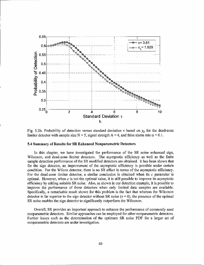
0.65

-e--c= 3.61C, 1.929

0 0.55 - - - - ------------

2- 0.35---------------

C 0.

"0.4 2-4 6 8i

o0.25 1

0 10

Standard Deviation -rb.

Fig. 5.3b. Probability of detection versus standard deviation 'T based on yg for the dead-zonelimiter detector with sample size N =5, signal strength A = 4, and false alarm rate cc = 0. 1.

5.4 Summary of Results for SR Enhanced Nonparametric Detectors

In this chapter, we have investigated the performance of the SR noise enhanced sign,Wilcoxon, and dead-zone limiter detectors. The asymptotic efficiency as well as the finitesample detection performance of the SR modified detectors are obtained. It has been shown thatfor the sign detector, an improvement of the asymptotic efficiency is possible under certaincondition. For the Wilcox detector, there is no SR effect in terms of the asymptotic efficiency.For the dead-zone limiter detector, a similar conclusion is obtained when its c parameter isoptimal. However, when c is not the optimal value, it is still possible to improve its asymptoticefficiency by adding suitable SR noise. Also, as shown in our detection example, it is possible toimprove the performance of these detectors when only limited data samples are available.Specifically, a remarkable result shown for this problem is the fact that whereas the Wilcoxondetector is far superior to the sign detector without SR noise ('r = 0), the presence of the optimalSR noise enables the sign detector to significantly outperform the Wilcoxon.

Overall, SR provides an important approach to enhance the performance of commonly usednonparametric detectors. Similar approaches can be employed for other nonparametric detectors.Further issues such as the determination of the optimum SR noise PDF for a larger set ofnonparametric detectors are under investigation.

40

6.0 Application of Stochastic Resonance to Imagery

6.1 Image Quality Metrics

In Phase I, a state-of-the art assessment was conducted on image quality metrics todetermine if they can provide an approximate and more efficient method of obtaining qualityscores provided by human observers. Important considerations involve image noise consistingof (a) random image noise such as impulsive and additive noise as well as (b) structural noiseconsisting of artifacts in the imagery. Another important consideration is the degradation ofimage sharpness due to blurring, ringing, and blocking effects. The advantages of the imagequality metrics is that they are able to dynamically monitor and adjust image quality, optimizeparameters and algorithms, and benchmark image processing systems and algorithms.

Objective quality metrics can be placed in three general categories. These consist of (a) fullreference, (b) no reference, and (c) reduced reference. Full reference metrics provide a so-called'perfect version' in the sense that 'ground truth' or a 'golden image' is available as a reference.Here, the image quality is measured by comparing the difference between the reference and thedistorted image. For the 'no reference' case, no such reference is available so that the imageitself must be assessed. Finally, the 'partial reference' methods utilize available partialinformation regarding the 'perfect image' as in the case of image fusion processing wheremultiple images are utilized.

Several image comparison metrics have been proposed to compare the similarity betweendifferent images. Among the most prevalent is the mean-squared error metric which is anaverage of the sum of squares of the pixel value differences between each image and is expressedas

1 N M

MSE = _- [X(, j)- Y(i.j)] 2 (6.1)AMz i=1 j=1

where X(i,j) and Y(ij) are the ijth pixel values for images X and Y, respectively.

Due to its important statistical meaning, Mutual Information (MI) is also widely used asan evaluation measure which is given by

I = H(X) + H(Y) - H(X, Y) (6.2)

where H(-) is the entropy. Although it can been shown that for I = H(X), Y is identical to X,

MI is not directly related to human perception performance; i.e., MI does not adequately indicatethe visual perception performance [Chen et al. 2005]. Also, since the calculation of MI involvesthe estimation of a joint PDF between X and Y, MI is often not suitable for a relatively smallsized image where the sample support is low. Alternatively, it is difficult to extend MI to handlea high dimensional image dataset. A related quantity, however, called the visual informationfidelity metric is considered below.

Structural Similarity (SSIM) [Z. Wang, et al. 2004], a nonlinear combination of thedifference in terms of the mean, variance, and contrast is also widely used and is expressed as

41

1 SSIMi (6.3)M j=1

where25ý-y + C, 2a'xy + C2 64

SSIM1 = Y2 +C (Y,2 (6.4)

The Visual Information Fidelity (VIF) has also been considered [Sheikh, Bovik, et al.2004]. It is a measure of the ratio

VIF = Di- (6.5)RU

where Di is the distorted image information and Ri is the reference image information. A signalgain and additive noise model in the wavelet domain given by

D=GC+V (6.6)

is applied to describe the test image, where C denotes the random field (RF) from a wavelet sub-band in the reference image and D denotes the corresponding signal in the test image. G is adeterministic scalar gain and V is white Gaussian noise. A Gaussian distribution assumption isthen made to calculate the mutual information. Overall, DiI and Ril are obtained as thesummation of the mutual information of all sub-bands between the distorted image and the trueimage C and between the reference image and C, respectively. Examples of the VIF metric areshown in Fig. 6.1 for VIF values of 1.0 (reference image), 1.1, 0.07, and 0.10.

Reference VIF = 1.0 Contrast Enhanced VIF = 1.10

Fig. 6.1 Examples of the Visual Information Fidelity (VIF) metric (continued on next page).

42

Blurred VIF = 0.07 JPEG Compressed VIF = 0.10

Fig. 6.1 (continued) Examples of the VIF metric.

The 'No-Reference (NR) Quality Assessment' algorithms [Z. Wang, et al., 2000], [Sheikh,et al., 2005] were recently developed to evaluate image quality without a reference image; i.e.,when no reference image is available. They are based on a quantization of the image distortion.Specifically, the edge sharpness level quantization relates to the edge width and the blur levelestimation and noise level estimation is affected by the impulse noise level and the additiveGaussian noise level. Some existing NR metrics consist of image ringing and blurring measures,image noise level, as well as receiver operating characteristic (ROC) curves as in medical imageprocessing where the detection performance of a certain disease is considered.

Finally, the Adaptive Image Quality Measure (IAQM) has been considered [Bingabr,Varshney, Farell, 2003] as a measure which provides the peak signal-to-noise ratio computedafter eliminating the errors not seen by the eye and the extent (in terms of percentage of blocks)to which the image is corrupted.

In future work, we will utilize such metrics to improve the filtered image quality anddetermine the best parameters for the SR based approach as in cases such as the median filteredimage discussed in Section 2.0. By doing so, automatic filtering algorithms will be developedand it is anticipated that performance will be improved over state-of-the-art methods.

6.2 Detection Enhancement in Imagery

We again emphasize that the specific form of the noise PDF plays a critical role to achieveenhancement via SR. We reconsider the problem addressed in [Kay 2000], but now for a two-dimensional (150x150 pixel) image. In Fig. 6.2, a 6x6 window is used to process the data so thatN = 36 pixels. Fig. 6.2a shows the original image with no additive noise while Fig. 6.2b showsthe image with additive Gaussian mixture noise. Fig. 6.2b is now used as the baseline observed

43

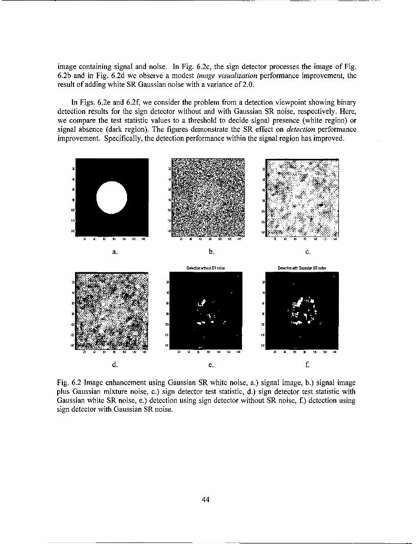
image containing signal and noise. In Fig. 6.2c, the sign detector processes the image of Fig.6.2b and in Fig. 6.2d we observe a modest image visualization performance improvement, theresult of adding white SR Gaussian noise with a variance of 2.0.

In Figs. 6.2e and 6.2f, we consider the problem from a detection viewpoint showing binarydetection results for the sign detector without and with Gaussian SR noise, respectively. Here,we compare the test statistic values to a threshold to decide signal presence (white region) orsignal absence (dark region). The figures demonstrate the SR effect on detection performanceimprovement. Specifically, the detection performance within the signal region has improved.

40

40 40

120 so 8

120 2012

140

20 40 M• 40 110 120 140 20 40 0 C 10O 20 140 20 40 4 40 1( 20 ) 1A

a. b. C.

Detecton without SR noise Detecton with Gaussian SR noise

23 20

40 40

40 e4

ý202f

IM 1ý 140140

20 AO 80 4 0 '10 120 142 20) 4 40 40 1M 120I 140 20 40 GO BO 120 120 140

d. e. f.

Fig. 6.2 Image enhancement using Gaussian SR white noise, a.) signal image, b.) signal imageplus Gaussian mixture noise, c.) sign detector test statistic, d.) sign detector test statistic withGaussian white SR noise, e.) detection using sign detector without SR noise, f.) detection usingsign detector with Gaussian SR noise.

44

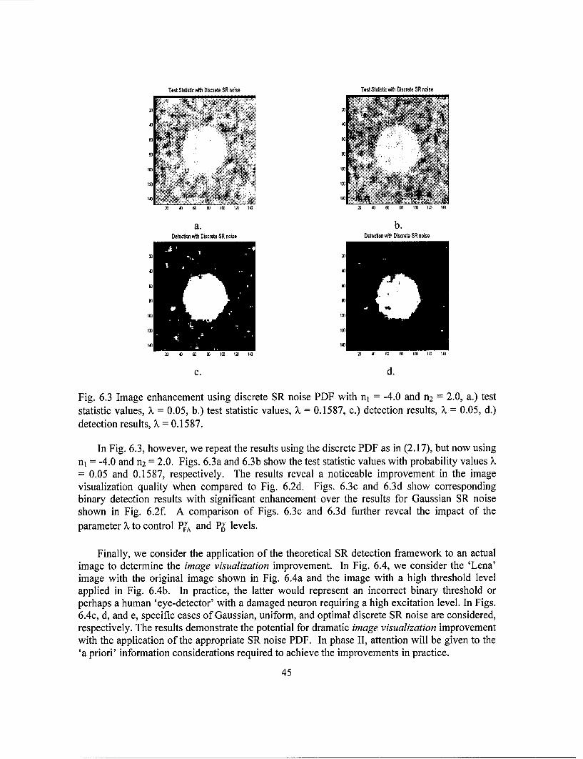
Test Staistic witt Discrete SR noise Test SO.stic with Discrete SR noise

a. b.Detection with Discrete SR noise Detection wii Discrete SR noise

01 40

100 00

120 101

0D AD ED ea 01 01 lAu &1 w 01 5 1 00 10 140

c. d.

Fig. 6.3 Image enhancement using discrete SR noise PDF with n1 = -4.0 and n2 = 2.0, a.) test

statistic values, 2, = 0.05, b.) test statistic values, 2. = 0.1587, c.) detection results, 2. = 0.05, d.)detection results, 2. = 0.1587.

In Fig. 6.3, however, we repeat the results using the discrete PDF as in (2.17), but now usingnl=-4.0 and n2 = 2.0. Figs. 6.3a and 6.3b show the test statistic values with probability values 2.

= 0.05 and 0.1587, respectively. The results reveal a noticeable improvement in the imagevisualization quality when compared to Fig. 6.2d. Figs. 6.3c and 6.3d show correspondingbinary detection results with significant enhancement over the results for Gaussian SR noiseshown in Fig. 6.2f. A comparison of Figs. 6.3c and 6.3d further reveal the impact of theparameter 20 to control P0 and PY levels.

Finally, we consider the application of the theoretical SR detection framework to an actualimage to determine the image visualization improvement. In Fig. 6.4, we consider the 'Lena'image with the original image shown in Fig. 6.4a and the image with a high threshold levelapplied in Fig. 6.4b. In practice, the latter would represent an incorrect binary threshold orperhaps a human 'eye-detector' with a damaged neuron requiring a high excitation level. In Figs.6.4c, d, and e, specific cases of Gaussian, uniform, and optimal discrete SR noise are considered,respectively. The results demonstrate the potential for dramatic image visualization improvementwith the application of the appropriate SR noise PDF. In phase II, attention will be given to the'a priori' information considerations required to achieve the improvements in practice.

45

MD

14, W] IM 3 ] D 3 3 3) 9) 1 50 2M 3 29) 3D 350 0) 4W3 03

a. b.

93 l3l93D3DD3D~9333 93193933DD3DD493933

10. d. e

FIg. 64IaevsaiainuIngte'eaSmgOa)oiia eaiagb)iaewthig thehl plec)GusanS osd)uiomSMoie . pia iceeSnoise.

M46

7.0 Application of Stochastic Resonance (SR) to Distributed Detection

Despite the progress achieved over the past two decades, the application of the SR effect todistributed detection has not been shown. Here, we investigate this application area for the dualhypothesis detection problem. We restrict ourselves to binary local sensor outputs, denoted byUk, and consider the cases of both conditional independence and dependence among sensorobservations. The degradation of detection performance caused by transmission errors betweenlocal sensor outputs and the fusion center is assessed. The relationship between the additive SRnoise and system performance is explored. For the traditional two-stage approach using theChair-Varshney fusion rule [Chairl986], the role of additive SR noise at both the decoding stageand the decision stage is discussed. We show that the SR phenomenon exists under certaincircumstances for both cases.

7.1 Stochastic Resonance Problem Statement

We again summarize the mathematical framework here for convenience. Given a K-dimensional data vector x E RK, we decide between two hypotheses Hi and Ho,

HO: px(x;Ho) = po(x) (7.1 a)Hi: p,(x;H1) = pl (x) (7.1 b)

where p0(x) and pi(x) are the pdfs of x under H0 and HI, respectively. In order to make adecision, a test that can be completely characterized by a critical function (decision function) 4where 0 < 4)(x) < 1 for all x, is required to choose between the two hypotheses. For anyobservation x, this test chooses the hypothesis H1 with probability 41(x). The detectionperformance of this test 4(() can be evaluated by its probability of detection PD and probability offalse alarm, PFA. In order to enhance detection performance, we add SR noise to the originaldata process x and obtain a new data process y given by

y = x + n, (7.2)

where the n is either an independent random process with pdfpn(.) or a nonrandom signal. Forthe case where the critical function 4(.) is fixed, to improve PD without increasing PFA, theoptimum SR noise has been shown to consist of no more than two discrete vectors [Chen2006a,fJ; i.e., the optimal SR noise pdf p°Pf (n) is of the following form,

p°Pt (n) =- A5(n -nl) + (1 - i2)8(n - n2) (7.3)

where 0 < X < 1, nj and n2 are suitable K dimensional vectors.

7.2 Decision Fusion and non-ideal Transmission Channels

A typical parallel fusion model with transmission channels is shown in Fig. 7.1. For the kthlocal sensor, an independent binary decision uk is made based on its observations. Without loss

47

of generality, assume that u. = 0 if H0 is decided and Uk = 1, otherwise. The detectionperformance of the kth local sensor node can be characterized by its corresponding probability offalse alarm and detection, denoted by PFAk and PDk, respectively. The kth local decision Uk is

sent to the fusion center through a transmission channel Ck characterized byp(xk Iuk). Yhe

final decision uo is made at the fusion center based on the received data x = [xi, x2, ... , XK]T and

the fusion rule y, i.e.,

U0 = Y( X1, X2, ... , XK). (7.4)

U1

PD9F2Sensor 2 U2 P X1 U )-2uso

PDK, PFAK -ISensor K P(IjK

Fig. 7.1 The parallel fusion model.

In general, two different fusion rules are applicable at the fusion center depending on thedifferent definitions of the output x. For the traditional two-stage approach, the output of eachtransmission channel Xk is the estimate ofuk; i.e., the kth channel can be described as a binary

channel with crossover error probabilities ak and 13k. The fusion rule yi, assuming perfectconnections between the local sensors and the fusion center, is given by

7. = log (1 PDk)PFAk > < ' (7.5)

Further, by applying the channel model for the signal detection problem for the kth local sensorand its corresponding channel Ck, the relationship between Xk and the hypothesis Hi can bedescribed as a two-layer transformation channel shown in Fig. 7.2 with its equivalent one-layermodel shown in Fig. 7.3. After accounting for channel errors, the equivalent kth sensorprobability of detection Pfk and probability of false alarm PCAk are given by

Pck = ( - P3 k) PDk + ck(l - PDk) (7.6)and

PPFAk = ( 1- 3 k) PFAk + Ok(l - PFAk)" (7.7)

48

Ho 1 - PFAk 1 0

P FA < Uk k<X1 - PDk Uk kXk

H1 11Pgk 1 13 k

Fig. 7.2 A two layer transmission channel model for a distributed detection system.

1- PEAk0

PCCHnp 1 - i i- 0

PcFA>k

PDk Xk

H1 "/" PC

P Dk

Fig. 7.3 Channel model for a signal detection problem in local sensor k.

Therefore, when the channel statistics Uk and 13k are available, the optimum fusion rule y2 at thefusion center is given by the Chair-Varshney rule [Chair 1986]

r2Elo (1-PX1kl) D k > (7.8)

When the channel is perfect, i.e., ctk = 3k = 0, we have P•, = PDk andPFAk = PFAk while =Y2 -- 1.

Compared to the two-stage fusion approach where the output of channel k is the binaryestimate of Uk, channel aware decision fusion rules have been developed recently [B. Chen2004], [Niu 2006] based on the direct observation of channel data. In this approach, the outputof channel Ck is no longer a binary variable but a continuous random variable. The exact form ofP(Xk I uk) depends on the coding rule at each local sensor and its corresponding noisy channelmodel. For example, for many wireless sensor network scenarios, the kth channel between thekth local sensor and the fusion center can be modeled as a unit power Rayleigh fading channelconsisting of additive Gaussian noise with variance o-2. Assuming that the local sensors send a1 when H1 is decided and -1 otherwise, the channel statistic P(Xk I uk) is given by

49

p(xk lu 1)- 20.k exp(--,(p k[ ,--- exp(akxk/2)Q(-akxk)], (7.9)P(2k I(1 + 2"k2) 2. L-

and2ak 2

P(Xk2I(Uk=) P (k/2)Q(akxk), (7.10)= 1 + 2a) 2 exp(_t

where ak 0.k (1+20.?) and Q(x) exp(-t2 /2)dt is the complimentary distribution

function of the standard Gaussian distribution.

Several decision fusion rules that require different degrees of a priori knowledge have beenproposed in [B. Chen 2004], [Niu 2006]. We summarize the test statistics for a few of themhere.

1. Chair-Varshney Fusion Rule

73 = E log(;FAk;Dk I(xk) (7.11)k=1 1_ (1 - Pok )PFAk

where I(.) is an indicator function

I(x) = OX Ox<O

2. Equal Gain Combining (EGC) Fusion Statistic

1KY4 =-EXk, (7.12)

k=l

3. Likelihood Ratio Test Based on Channel Statistics (LRT-CS)

These test statistics are based on the knowledge of channel statistics and local detectionperformance indices

Ks = log 1 + / 2;/akxk exp(akxk2/ 2)Q(-akxk) (7.13)k=1lo 1- -,2I-7rakxk exp(akxk / 2)Q(akxk) J

50

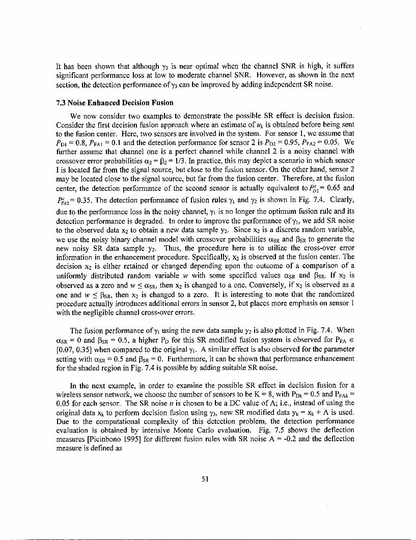
It has been shown that although y3 is near optimal when the channel SNR is high, it sufferssignificant performance loss at low to moderate channel SNR. However, as shown in the nextsection, the detection performance of ' 3 can be improved by adding independent SR noise.

7.3 Noise Enhanced Decision Fusion

We now consider two examples to demonstrate the possible SR effect is decision fusion.Consider the first decision fusion approach where an estimate of Uk is obtained before being sentto the fusion center. Here, two sensors are involved in the system. For sensor 1, we assume thatPD1 = 0.8, PFA1 = 0.1 and the detection performance for sensor 2 is PD2 = 0.95, PFA2 = 0.05. Wefurther assume that channel one is a perfect channel while channel 2 is a noisy channel withcrossover error probabilities (X2 = P32 = 1/3. In practice, this may depict a scenario in which sensorI is located far from the signal source, but close to the fusion sensor. On the other hand, sensor 2may be located close to the signal source, but far from the fusion center. Therefore, at the fusion

center, the detection performance of the second sensor is actually equivalent to PD2= 0.65 and

PF.2= 0.35. The detection performance of fusion rules 71 and 72 is shown in Fig. 7.4. Clearly,

due to the performance loss in the noisy channel, yj is no longer the optimum fusion rule and itsdetection performance is degraded. In order to improve the performance of 'y, we add SR noiseto the observed data x2 to obtain a new data sample Y2. Since x2 is a discrete random variable,we use the noisy binary channel model with crossover probabilities cLSR and P3SR to generate thenew noisy SR data sample y2. Thus, the procedure here is to utilize the cross-over errorinformation in the enhancement procedure. Specifically, x2 is observed at the fusion center. Thedecision x2 is either retained or changed depending upon the outcome of a comparison of a

uniformly distributed random variable w with some specified values cxSR and PSR. If X2 isobserved as a zero and w < CCSR, then x2 is changed to a one. Conversely, if x2 is observed as aone and w _< 3SR, then x2 is changed to a zero. It is interesting to note that the randomizedprocedure actually introduces additional errors in sensor 2, but places more emphasis on sensor 1with the negligible channel cross-over errors.

The fusion performance of yl using the new data sample y2 is also plotted in Fig. 7.4. WhenCtSR = 0 and [3SR = 0.5, a higher PD for this SR modified fusion system is observed for PFA E

[0.07, 0.35] when compared to the original y'. A similar effect is also observed for the parametersetting with UCSR = 0.5 and P3SR = 0. Furthermore, it can be shown that performance enhancementfor the shaded region in Fig. 7.4 is possible by adding suitable SR noise.

In the next example, in order to examine the possible SR effect in decision fusion for awireless sensor network, we choose the number of sensors to be K = 8, with PDk = 0.5 and PFAk =

0.05 for each sensor. The SR noise n is chosen to be a DC value of A; i.e., instead of using theoriginal data xk to perform decision fusion using y3, new SR modified data Yk = Xk + A is used.Due to the computational complexity of this detection problem, the detection performanceevaluation is obtained by intensive Monte Carlo evaluation. Fig. 7.5 shows the deflectionmeasures [Picinbono 1995] for different fusion rules with SR noise A = -0.2 and the deflectionmeasure is defined as

51

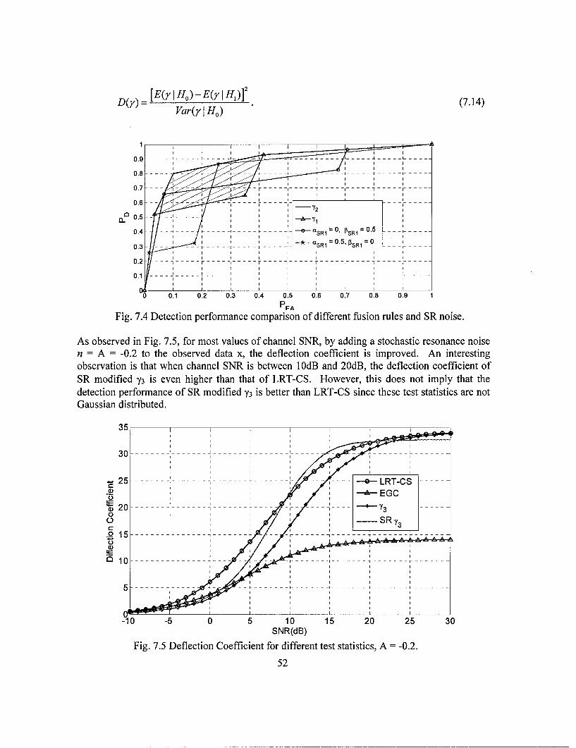
D(y)- [E(y Ho)-E- E(O' )]2 (7.14)Var(y Ho)

I I I

0.9 - -. .. . . . ,-.

0.8 --- -- - - -......

I I - yi

C ' 0 . - -- J - - - --IL-- --- --. . .S i I i I I

0.4 -- 2--- SRI = =0.5- =-* I I I

0.3- - - - - SRI = 0 5

'PSR1 0 ----------I I I I I

0 .2 - - i -- -- -* t I I Iii0.2 2 I

0 .1 - -- - , - -S I I i I i I

I I II I

0 0.1 0.2 0.3 0.4 0.5 0.6 0.7 0.8 0.9

PFA

Fig. 7.4 Detection performance comparison of different fusion rules and SR noise.

As observed in Fig. 7.5, for most values of channel SNR, by adding a stochastic resonance noisen = A = -0.2 to the observed data x, the deflection coefficient is improved. An interestingobservation is that when channel SNR is between 10dB and 20dB, the deflection coefficient ofSR modified y3 is even higher than that of LRT-CS. However, this does not imply that thedetection performance of SR modified 73 is better than LRT-CS since these test statistics are notGaussian distributed.

35

30-/ -- -- - -- - -- - -- - --- --

S25 ----- ----- ---- --- LRT-CS ------C : _,,, . I ' EGc I

.0 15 --- - - - - - -- - - - - .. .. -- --- --- ---.----. ......-d)

20 .....

Fig 75DfetoCofiinfrdiffrn tes sttsics A 02

~~52

C.) Ii

-0 -0 5 10 15 20 25 30SNR(dB)

Fig. 7.5 Deflection Coefficient for different test statistics, A = -0.2.

52

For a fixed channel SNR and SR enhanced y'3 decision fusion, the relationship betweendifferent values A and deflection coefficient D is shown in Fig. 7.6. As A starts becomingnegative, the deflection coefficient D first increases and then, after attaining its peak, decreasesas A decreases further. The optimum value of A, namely A0, which maximizes D is an increasingfunction of SNR. When SNR is very high, we have A0 z 0 which is consistent with theconclusion drawn in [B. Chen 2004], [Niu 2006] where the asymptotic optimum of 'Y3 is derived;i.e., SR noise will not improve performance at high SNR.

3 5.....

-1 -0. -0. 04 -. . 0. 0. 0.

30 7.6-Deflect-io cofiin f SNR = 5dB - c- -,, nel. NRdB.Clearly , theSR modi es a be d p

"t- 25 -- -- ,' -___- ------ -- - - - -.. . .. ..'* SNR = 25dg -- ,-- -

(D 2 0 -- -- --- --- -- --- -- -.-- - -- - ---- -. --- --.- - -

0 i , we fi t in h r tio

trnsisio hane ilstatd n i. .2 w av fri~

o 5 --- --.--.--- --- --- --.--.-.--- --- .-- --

k- -(Iy -OI -=1 - - 0!y 0 ... U4 .6 0.. (7.1iB ClalteS oiieY3fso r ul proide aetrdtcio pefrac hnbt

Fronmiso (9) and e (10),uaterasoed calculation, we havefoy,

iX = Pi(k = I I Uk=0,(.5

0k =P IYk = Ojk = 1) = I -P k = 1U 1-(.6

From (9) and (10) afterinale ' alrulatowe.v

P(I(yk) = lI uk = 1) p((xk + A) -P1 Uk = 1)

53

=p(Xk --> -Al Uk = 1)f127l2+2- xp(_ 2 Ii+_ V akt exp(at 2 / 2)Q(-akt)?t

=-A (+20)

Q A Q(Aak) exp (7.17)-k - 1f+-20- 1i +2-2

and

P(I(yk)= llUk=O)= I-Q -•A Q(-Aak) e1p A 2 (7.18)Uk /1 + -2,7k- ( 1 +-20-k

From (17) and (18), it can be shown that cXk monotonically decreases and 13k monotonicallyincreases as A decreases. An illustration of such relationship is shown in Fig. 7.8 for the case ofchannel SNR = 5dB. Also, from (6) and (7), it can be shown that for any fixed channel SNR andprobability of false alarm PFA, the probability of detection PD given by the SR modified fusionrule 'y3 is determined by the crossover error probabilities Ck and 13k, k = 1, 2, ... , K which arefunctions of A. Therefore, there exists a suitable A which yields the best detection performance,

i.e., maximizes the PD for a given PFA. When A = 0, Cxk = P3k = 12- 1 - ' When SNRY2 -ý2ý 1+ 2g

is very high, ak, 13k -> 0, and the channel Ck becomes a near perfect channel. As a result, Y3becomes a near optimum fusion rule.

1 I I IPP IPP I I PP P1111 P I I PIIl0 . -- - -l - I I I ll 1 I I 1 4 lilt I I - e I IllII I I r• IPI I I I 11111l I I I I11 I I I iii

I I I!1li111 I I P 1 1 1P P 1 1 IIP

0.- ------ oSmm ----- r-r-----TT-P-,-- -=-,---r-PmP 1111 PI P I IPI I PI 11 P PIl P PI P

10P l 1 1 I1I I10

a P II1I

P FAPFg 7..7 RO curve for " vaiu fuio sttsis SRR A - .2 ..

4 III

PI P P 1 P 11 1 P P P 1111 P P uI I P P 111SI I PIl I IP I I I P I 1 11 I I Jill1 I P 1 I I III11 1 P P PP IP P P IP I P P P II 11 11 P P IIIII

P I I11 1 I I 1 11 I P I IP P P P 11111 I P I I I I

PFA

Fig. 7.7 ROC curves for various fusion statistics; SNR = 5dB, A = -0.2.

54

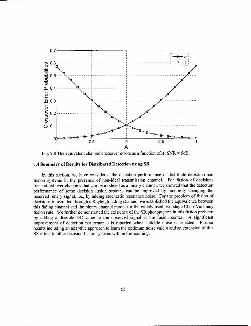
0.7

cn 0.6 ------ --.--- -------------- 4-- -

0. 0

0

L.

W. 0.3 - ---------------------------------------- -------0

LU 0.3

0. ------ -4--------------------- ----- 4--------

-1 -0.5 0 0.51A

Fig. 7.8 The equivalent channel crossover errors as a function of A, SNR = 5dB.

7.4 Summary of Results for Distributed Detection using SR

In this section, we have considered the detection performance of distribute detection andfusion systems in the presence of non-ideal transmission channel. For fusion of decisionstransmitted over channels that can be modeled as a binary channel, we showed that the detectionperformance of some decision fusion systems can be improved by randomly changing thereceived binary signal, i.e., by adding stochastic resonance noise. For the problem of fusion ofdecisions transmitted through a Rayleigh fading channel, we established the equivalence betweenthis fading channel and the binary channel model for the widely used two-stage Chair-Varshneyfusion rule. We further demonstrated the existence of the SR phenomenon in this fusion problemby adding a discrete DC value to the observed signal at the fusion center. A significantimprovement of detection performance is reported when suitable noise is selected. Furtherresults including an adaptive approach to learn the optimum noise vale n and an extension of thisSR effect to other decision fusion systems will be forthcoming.

55

8.0 Optimal Decision Processing by the Transformation Method

For decision problems whose decision region is suboptimal, we now show how to transformthe decision statistic to recover optimal performance [Kay, 2006a]. This novel methodologyholds considerable promise in a wide range of application areas involving decision theory. Theprocedure simply amounts to transforming the decision statistic to yield a combinedstatistic/decision region which is optimal. The approach may be thought of as a generalization ofthe stochastic resonance phenomenon, which employs a random linear transformation, and henceshould be widely applicable to many practical problems. Maximization of the probability of acorrect decision, as considered here for example, has direct applications to communicationtheory. The method considered here treats the univariate case. Its generalization to themultivariate case will be considered in future work.

8.1 Mathematical Description of the Transformation Method

A mathematical justification of the approach is given in this subsection with an example inthe next subsection. Here, we assume that the problem is to decide between two hypotheses Hoand H1 based on the observed scalar test statistic x. The two hypotheses are assumed to berandom events with prior probabilities of no and 7r1. This test statistic is a function of the originaldata. A future problem will address the extension to the case when the original data isaccessible. Based on the observed data sample x, a decision rule has been implemented asfollows:

ý(x) = 1 decide i (8.1a)

4(x) = 0 decide Mo. (8.1b)

This decision rule is assumed to be suboptimal. Denoting the probability density functions(PDFs) as px (x) and pX (x) under Ifo and Y1j, respectively, the probability of a correct decision

is

S= o fE (1 - q(x))px (x)dx + g, fE (x)pX (x)dx

= go + E (w)P' piX (X)-)Top6x (x)]dx (8.2)

Note that unless 4(x) = 1 for all x such that that irlpX (x) -;ropx (x) > 0 and zero otherwise

(which is the optimal decision rule) this probability will not be maximized.

Now consider that we transform the test statistic as y = g(x) using some function g. Thefunction is assumed to be piece-wise monotonic so that over each interval of a finite number ofdisjoint intervals either g'(x) Ž_ 0 or g'(x) < 0 (the prime denotes differentiation). The

transformed test statistic y is then input to the decision rule 4(.) to yield 4(y). This is inaccordance with the assumption that the decision rule is fixed and so cannot be changed. Onlythe test statistic can be modified. We will see, however, that this is mathematically equivalent tomodifying the decision rule. To do so note that P., which is now based on y, is

56

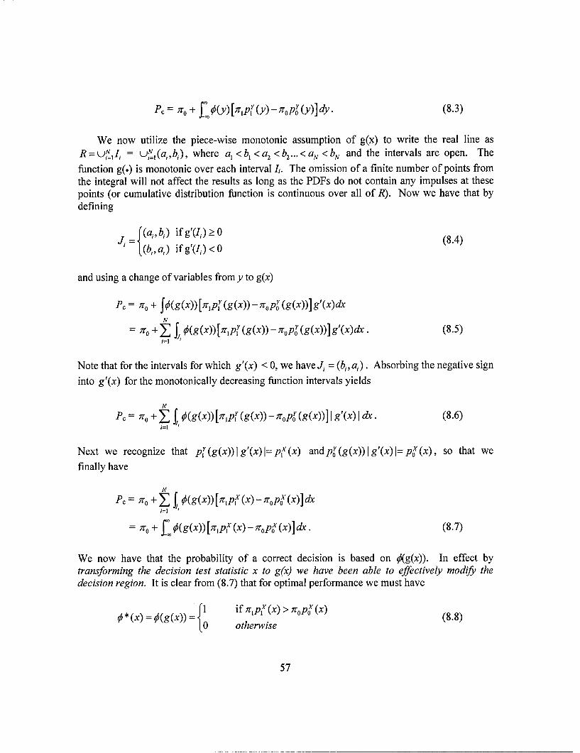
PC = go + f•0(y) [Prpr (Y)-goPr (y)] dy. (8.3)

We now utilize the piece-wise monotonic assumption of g(x) to write the real line asR= uNIi = uN, (a,,b,), where a<b < <a b <.aN <b. and the intervals are open. The

function g(.) is monotonic over each interval Ii. The omission of a finite number of points fromthe integral will not affect the results as long as the PDFs do not contain any impulses at thesepoints (or cumulative distribution function is continuous over all of R). Now we have that bydefining

-= r(aj, b) ifg'(Ij) > 0 (8.4)

- L(b,,a,) ifg'(I,) < 0

and using a change of variables from y to g(x)

PC= )TO + fr3(g(x))[g 1pr (g(x))- opr (g(x))]g'(x)dxN

=o + Z f. 5(g(x))[i7rpr (g(x))- opr' (g(x))]g'(x)dx. (8.5)i=1

Note that for the intervals for which g'(x) < 0, we have J, = (bi, a,). Absorbing the negative sign

into g'(x) for the monotonically decreasing function intervals yields

N

Pc = go + o j qi(g(x)) [gipl' (g(x))- -opr (g(x))] I g'(x) I dx. (8.6)i=l

Next we recognize that py(g(x))Ig'(x)l=px(x) andpr(g(x))lg'(x)j=pox(x), so that we

finally have

NPc = o +~ j', (g(x))[;lpjx'(x)-;opox(x)]dx

=o + fq5(g(x))[gTplx (x)- gopox (x)] dx. (8.7)

We now have that the probability of a correct decision is based on z(g(x)). In effect bytransforming the decision test statistic x to g(x) we have been able to effectively modify thedecision region. It is clear from (8.7) that for optimal performance we must have

0 * (x) = O( g(x)) otherwise (8.8)

57

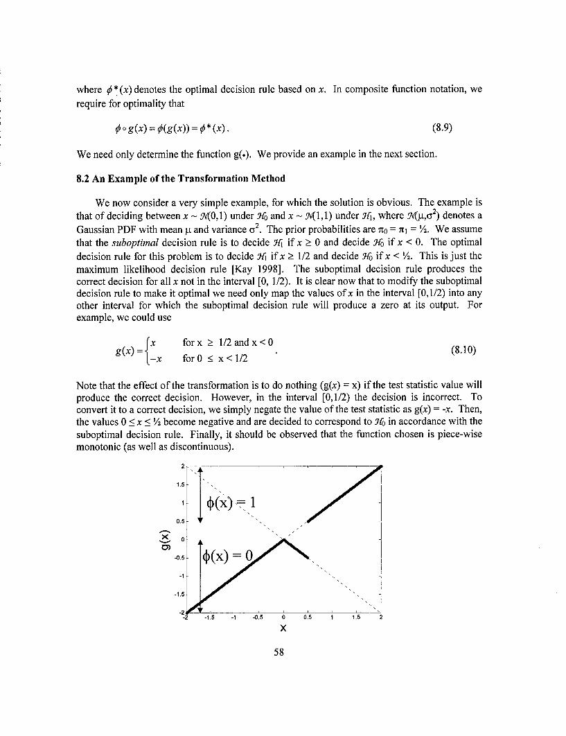
where 0' (x) denotes the optimal decision rule based on x. In composite function notation, we

require for optimality that

0 o g(x) = •z(g(x)) = 0 * (x). (8.9)

We need only determine the function g(.). We provide an example in the next section.

8.2 An Example of the Transformation Method

We now consider a very simple example, for which the solution is obvious. The example isthat of deciding between x - 9V(0,1) under YfO and x - 9V(1,1) under 3Tj, where gv(Na2) denotes a

Gaussian PDF with mean ji and variance a2. The prior probabilities are 70 = 71 = V2. We assumethat the suboptimal decision rule is to decide Hl1 if x _> 0 and decide 5%i if x < 0. The optimal

decision rule for this problem is to decide Yfi if x _> 1/2 and decide 5%b if x < 72. This is just themaximum likelihood decision rule [Kay 1998]. The suboptimal decision rule produces thecorrect decision for all x not in the interval [0, 1/2). It is clear now that to modify the suboptimaldecision rule to make it optimal we need only map the values of x in the interval [0,1/2) into anyother interval for which the suboptimal decision rule will produce a zero at its output. Forexample, we could use

x for x >1/2 and x< 0

g(x)={X forx 1/a (8.10)x for0 < x<1/2

Note that the effect of the transformation is to do nothing (g(x) = x) if the test statistic value willproduce the correct decision. However, in the interval [0,1/2) the decision is incorrect. Toconvert it to a correct decision, we simply negate the value of the test statistic as g(x) = -x. Then,the values 0 < x < V2 become negative and are decided to correspond to Yf% in accordance with thesuboptimal decision rule. Finally, it should be observed that the function chosen is piece-wisemonotonic (as well as discontinuous).

2

1.5

1 -~x=1

X 0

-1-0.5

"25 -. 5 -1 -0.5 0 '05 1 15 2

x

58

Figure 8.1 Transforming Function - One of many possibilities.

9.0 Recommendations and Future Considerations

9.1 Extensions to the Optimized SR Detection and Estimation Framework

a. Optimized SR Detection Framework for the Unknown PDF Problem

In our Phase I effort, as discussed earlier, we have addressed the problem of using SR toimprove detection performance for the case when the probability density functions (PDFs) underthe two hypotheses are known. In future work, the emphasis must now be placed on the problemof adaptive learning and training of SR modified detectors in the unknown PDF case. For anyspecific test, we assume that the prior probabilities of both hypotheses are known and that wehave the knowledge of the model of this detection problem. Therefore, given a set of testingsamples, the underlying PDFs for the two hypotheses detection problem may be determined bystatistical learning methods [Vapnik 1996]. Furthermore, this learned PDF/CDF can beemployed further to construct a better detector or to improve the detection performance of thedetector obtained by the SR approach introduced in two of our papers [Chen, et. al., 2006a, b]developed during Phase I. Other model based learning algorithms such as the Ozturk algorithm[Ozturk, 1992] developed at Syracuse University (used to learn the distribution model) and theEM algorithm (used to learn the parameters of a certain model) shall also be explored. Theinformation extracted from data via these methods will be further utilized to determine the formof the optimum SR noise distribution for the detection problem under consideration.

b. Variable Decision Functions

In our prior work in Phase I, the test statistics as well as the detection threshold wereassumed fixed. Extension of the SR formulation of the fixed test statistic and detection thresholdcase to the variable threshold and variable statistic case will be pursued. Let D denote the set ofall possible test statistics, 9 be the set of all possible thresholds and 17 be the set of all possibleSR noise PDFs. For a Neyman-Pearson detection approach, we know that for any fixedprobability of false alarm PFA, its corresponding PD can not be greater than 1. Thus, there mustexist at least one (4,0,7t)e(D,4,,1) that maximizes the PD with false alarm rate less than or equalto PFA. The same conclusion can also be drawn for the Bayesian case. From our work reported in[Chen, et al., 2006a] and [Kay, et al., 2006], we have: 7t = pn(X) = 5(x-c) for the Bayesianapproach and 71 = Pn(X) = X8(x-d) + (1-X)8(x-f) for the NP approach. The next step of ourproposed Phase II effort in this area is to establish some relationships among 4, 0 and it for thevariable decision function and to further simplify the procedure to find the best SR detectionsystems.

c. Optimum SR Noise Considerations under Constraints

In some practical applications, additional constraints on SR noise may be applicable. Forexample, in a wireless sensor network (WSN), the power consumption at each sensor is aconcern. In this case, we would want to know the form of optimum SR noise PDF if the detector

59

or sensor's power is limited. This important case of SR noise under potential constraints will be

investigated.

d. Optimum SR Noise for the Multiple Hypotheses Test

In our prior work in Phase I, we focused our attention on binary hypothesis testing problemswith considerable success. We now intend to extend our results to the multiple hypothesestesting problem. This problem is encountered in classification problems in various applicationssuch as target identification, medical imaging, and remote sensing. As is well known fromstatistical decision theory, due to the complexity of the problem and unlike the two hypothesestest, the optimum solution of a multiple hypotheses test is very difficult to determine. The formof the optimum decision regions is not rectangular in general and in many cases non-optimumrectangular decision regions are employed. Therefore, our SR approach may play a veryimportant role in this case. The role of SR has not been investigated in this context. In futureanalyses, we will seek to determine the form of the optimum SR noise distributions for thisimportant case.

e. Robust Nonlinear Systems and Robust SR Noise

In the Phase I study, we evaluated the detection performance of certain detectors by addingindependent SR noise provided the PDF for each hypothesis is known and fixed. In the next stepof our research, a set of nonlinear systems will be considered and their robustness subject tosmall variations of the input signals will be evaluated. The relationship between the nonlinearsystem and SR noise from the viewpoint of robustness shall be explored.

f. SR Enhanced Signal Estimation

Dithering related techniques (in the SR sense) have been widely used in preserving signalinformation before AC to DC quantization or some other forms of transformations(preprocessing) [Wannamaker, 2000]. The quantized/transformed signal is then used as the inputto various signal processing systems (post processing). However, due to the fact that manysignal processing systems are nonlinear, the quantized/transformed signal may not be the optimalinput for certain kinds of systems. This is mainly due to the following two reasons: 1. The SRnoise in the preprocessing part may not be optimum. 2. There may exist a mismatch between theSR noise modified preprocessed signal and the signal processing system that follows; i.e., the SRnoise and its related preprocessed signal may be the optimum signal for one post processingsystem, but may not be optimum for another. Thus, it is a very important and interestingproblem as to how to tune the preprocessed signal again by adding SR noise or by some othermethods. As an example, in some preliminary work, we have demonstrated the existence of suchan SR phenomenon in a system where maximum likelihood estimation (MLE) is applied toestimate the signal parameter from the 1-bit quantized data. This notion will be investigated inmore detail for a wider class of problems and a systematic theory for estimation problems will bedeveloped just as we have initiated the theoretical formulation for detection problems in ourPhase I work.

g. Numerical Approaches to Optimum SR Noise PDF Determination

60

Numerical optimization approaches will be pursued to obtain an optimal solution of SR noisePDF. As shown in our previous results, the theoretical optimum SR noise PDF is shown to be asingle impulse for the Bayesian approach and two-peak noise for the NP approach subject to aconstant false alarm rate (CFAR) constraint. It is relatively easy to obtain the solution for thesingle dimensional problem. However, for higher dimensional problems, it is much moredifficult to find the solution. Thus, a set of numerical approaches including but not limited toGenetic Algorithm, Simulated Annealing and Particle Swarm Optimization techniques need to beexamined for potential use for this problem. We plan to conduct a study and characterize theefficacy of different optimization algorithms for SR problems.

h. Nonlinear Stochastic Resonance

The concept of SR will be extended to a much broader context. So far, we have restrictedourselves to the additive form of SR noise; i.e., we have only considered y = x + n. Here, wewill consider the case where the noise can actually take any functional form, i.e., we will extendit to the more complicated case where y is a function of input x and noise n, such that y = f(x,n).For example, we may consider a SR noise modified observation model to be multiplicative, i.e.,y = n*x. Further, instead of considering only one source of noise, multiple noise sources can beconsidered. For example, we could have a multiplicative part and the other an additive part. Onesuch kind of noise model is applicable when a signal is transmitted over a Rayleigh fadingchannel where y = nl*x + n2. The detection performance, the optimum solution and theperformance bounds for these more general SR schemes will be investigated with improvedperformance anticipated.

L. Detection Enhancement in the Presence of Correlated Non-Gaussian Noise

Further consideration should also be given to performance improvement to be realized bySR applied to nonparametric detectors for the problem of signal detection in correlated non-Gaussian noise and additive white Gaussian noise. Here, the bimodal models considered inPhase I shall be generalized to the multi-modal compound Gaussian model. Further, a verygeneral class of non-Gaussian processes known as Spherically Invariant Random Processes(SIRP) [Yao, 1973] shall be considered. The theory of SIRPs provides an elegant andmathematically tractable approach for the generation of multivariate non-Gaussian PDFs. Issuessuch as detection performance robustness and estimation efficiency (i.e., sample support size) areessential for these analyses.

There are two types of models for correlated non-Gaussian processes: (1) the endogenousmodel and (2) the exogenous product model [Conte, 1987]. For the endogenous model, thedesired non-Gaussian PDF and correlation function is realized using a zero memory, non-lineartransformation on a real Gaussian process. In this approach, however, it is not possible tocontrol both the PDF and the correlation independently [Rangaswamy, 1993]. Further, thenonlinear transformation may give rise to non-Gaussian processes with a non-negative definitecovariance matrix. For the exogenous model, however, the desired non-Gaussian process isgenerated by the product of a Gaussian random process and an independent non-Gaussianprocess which can be correlated. Thus, the PDF and correlation can be independently controlled.

61

This feature provides an important capability for both detection and estimation performanceassessments. Issues such as detection performance robustness and estimation efficiency (i.e.,sample support size) are of prime interest for these analyses.9.2 Optimal Decision Processing by the Transformation Method

The derivation of the transformation method discussed in Section 4.0 will be extended to themultivariate case in the future. Specifically, the more general case of data vectors of length Nshall be considered. This will allow the application of the approach to the more general problemwhen multi-sample data is available. The choice of the g(.) function is the critical issue here. Intheory, it is always possible to choose an appropriate function to implement the optimalmapping. However, in practice, if we are within a high-dimensional space, it may not be obvioushow it is chosen. We plan to investigate this approach as well as a possible extension to the caseof random transformations. The usual SR method may be thought of as a random transformationthat is effected by adding a random variable to the data. However, the restriction to an additionmeans that the transformation is constrained to be linear. Clearly, this is so restrictive as toimpede the possible implementation of an optimal decision rule. Our approach will alleviate thisrestriction.

9.3 Stochastic Resonance in Imagery

a. Image Quality Metrics

As noted previously, important image processing considerations involve image noiseconsisting of (a) random image noise such as impulsive and additive noise as well as (b)structural noise consisting of artifacts in the imagery. Another important consideration is thedegradation of image sharpness due to blurring, ringing, and blocking effects. The advantages ofthe image quality metrics is that they are able to dynamically monitor and adjust image quality,optimize parameters and algorithms, and benchmark image processing systems and algorithms.

Future work should further consider the image metrics noted in Section 6.1. We shall utilizethe appropriate metrics to assess improvement of the filtered image quality and determine thebest parameters for the SR based approaches as in cases such as the median filtered imagediscussed in Section 7.0. By doing so, automatic filtering algorithms will be developed and it isanticipated that performance will be improved over current state-of-the-art methods.

b. Noise Reduction

In our prior work in Phase I, it has been shown that SR can help to improve the noisefiltering performance in image processing. In particular, in [Chen, et. al., 2006d], we have shownthat SR noise can improve the performance of median filtering. This provides us the motivationto apply SR to a much broader class of image filtering and restoration problems for improvedhuman visualization. In unreported work, we have further demonstrated the existence of the SReffect for an image corrupted by Gaussian noise. Our preliminary experiments show that theperformance of Wiener filters improved when suitable SR noise is added. This is veryencouraging since Wiener filters are optimal for the Gaussian noise case with a stationary signal.The reason for such improvement is the fact that the assumption of stationarity does not usually

62

hold in images even for a small local region and almost all images are non-stationary, i.e., theircontent varies depending on location. In the future, we should focus on the derivation of theoptimum solution of the SR noise PDF for a large class of image enhancement problems.Emphasis should be placed on the development of efficient algorithms, possibly including anadaptive self-learning algorithm, to find the optimum SR noise for image filtering applications.

c. Image fusion

Image fusion, an important image processing technique to integrate useful information fromdifferent input images, has been widely used in a number of applications such as remote sensingand medical image processing. Among all of the image fusion algorithms, wavelet based multi-resolution image fusion is the most popular and powerful approach. One critical and difficultaspect in such an approach is to determine the fused image wavelet coefficient values. A numberof algorithms have been developed to tackle this problem. Future work should focus on how touse SR to improve image fusion quality, namely, how the SR noise can play a role to betterselect the wavelet coefficients as well as to determine the suitable neighborhood for an improvedfused image. The image quality will be evaluated based on image quality metrics (see Section6.1) that we have developed based on the human visualization system. Thus, a SR based imagefusion framework will be developed and its performance evaluation will be carried out.

d. Target Detection and Identification in Images

An important future consideration for SR enhanced detection is the extension of the currenttechniques from single pixel detection (the circular image of Fig. 6a) to more general targetdetection based on image data. One immediate application is to use SR to enhance templatematching for target detection, i.e., given a grey/color image I and a target template X (forexample, a face, a building or a military target, the template itself may be a simple binary image,a grey scale image, or a color image), the goal will be to search for the template in the entireimage. To find the existence and position of X in the given noisy image Y, a template matchingtechnique is often used; i.e., moving X on Y and attempting to find the peak of a similaritymetric such as the correlation function or mutual information. This is similar to matchedfiltering in a single dimensional problem. As Y often appears to be a grey image, one wouldexpect some error and considerable computational burden as we try to find the template X in theimage Y directly when Y is a noisy image and/or the matching algorithms are sensitive to thesmall variations in the grey levels. The problem is actually similar to the image registrationproblem in which Syracuse University has considerable experience. Therefore, in this problem,quantization (or segmentation) of Y may become a very important preprocessing step.Furthermore, we would expect the SR effect (both in quantization and after quantization) tooccur in a similar manner as in SR enhanced median filtering. The potential for improvementmay be significant. A variety of applications can be pursued within this framework. These mightinclude face recognition, image registration (to improve the performance via registration aftersegmentation) and may even be applicable to the single dimensional problem.

63

9.4 Stochastic Resonance in Image Visualization

a. Enhancement of RGB Imagery

In our prior work in Phase I, it has been shown that the quality of the thresholded 'Lenna'image can be improved by adding a suitable two-peak noise. In future studies, the optimal noisefor a noisy image should be determined where the reference image is no longer available. Tobetter utilize the spectral as well as the spatial information, some image models such asmultiple-dimensional Markov Random Field models will be developed to better describe thecorrelations between R, G and B (red, green, blue) bands to further improve the image quality.Performance evaluation as well as adaptive learning algorithms will be pursued.

b. Multi- and/or Hyperspectral Imagery

In this area, the potential of improving Remote Sensing (RS) detection performance as wellas classification accuracy via SR will be explored. Our preliminary results show that suitableGaussian SR noise can improve the accuracy of the Gaussian Maximum Likelihood Classifier(GMLC). The role of SR in this area will be further examined utilizing the extensive techniquesdeveloped at Syracuse University [Varshney and Arora, 2004]. Possible enhancement of otherprocessing algorithms by adding SR noise will also be evaluated. The form of suitable SR noisefor specific algorithms will be derived.

c. Hyperspectral Image Visualization

Principal Component Analysis (PCA) and Segmented PCA (SPCA) based image visualizationtechniques [Tsagaris, 2005] are widely used to condense the information contained inhyperspectral images. However, due to the non-Gaussian nature of the hyperspectral images,PCA and SPCA may not fully utilize the hyperspectral imagery information. Moreover, PCAbased techniques may introduce some artifacts. In general, a universal optimal method to displaythe contents of the hyperspectral images does not exist. Therefore, in future analyses, thepotential enhancement by SR in various visualization schemes will be pursued and a bettervisualization result is expected.

d. Enhancement of Region of Interest (ROI)

Determination of the region of interest (ROI) is an essential part of many applications suchas the determination of possible location of tumors in medical images and the possibletarget/incidents in video surveillance. For these types of problems, description of the statisticalproperties of the ROIs to specify the exact form of the target distribution is generally impossible,although some features may be available. In future studies, SR based techniques should bedeveloped to better extract the features from the image and determine the location and size of theROIs. This approach will have a very broad application in medical image processing.

64

9.5 Visual Image Fusion Considerations for Human Perception

The rapid development in imaging and computing technology has fostered utilization ofvisual information for situation assessment and decision making. Multiple image devices ofeither the same or different modalities are used to capture images. These images are then fused tointegrate each image's information content to render a single image of enhanced quality. Asimage fusion techniques become available, evaluation of their performance is of high interest.However, there is a requirement for specific metrics to evaluate the quality of fused images andits affect on the human vision system (HVS). This problem has been addressed at SyracuseUniversity [Chen and Varshney, 2006]. For the current proposal, such algorithms may bepertinent to the fusion of multiple images each containing an IID realization of added noise.

Comparative evaluation of fused images is a critical step to evaluate the relativeperformance of image fusion algorithms. Human visual inspection is often used to assess thequality of fused images. Here, we discuss some variants of a new image quality metric based onthe human vision system (HVS). These measures evaluate the fused image quality by comparingits visual differences with the source image thus requiring no ground truth knowledge. First, theimages are divided into several local regions. These regional images are then transformed to thefrequency domain. Second, the difference between the transformed local regional images isweighted with a human contrast sensitivity function (CSF). The local regional image quality isobtained by computing the mean square error (MSE) of the weighted difference of the imagesobtained from the fused regional image and source regional image. Finally, the quality of afused image is the weighted summation of the local regional image quality measures. Ourexperimental results show that these metrics are consistent with perceptually obtained results.

The design of a universal objective measure for image quality is difficult due to the largevariety of image fusion applications. Often, ground truth images are not available so that imagequality evaluation is complicated. Since humans are the final users of fused images, humanvisual inspection is often used as the quality measure. However, human inspection may notalways be possible due to large input and output data sizes and associated financial costs. Severalautomatic image evaluation algorithms have been developed recently. A performance measurefor pixel-level fusion performance that compares the edge information of fused images with edgeinformation of input images has been proposed [Xydeas, 2000]. Later, it was used to calculatethe affect of noise on image fusion [Petrov, 2003]. Mutual information was also employed toevaluate fusion performance [Qu, 2002]. Wang and Shen [Wang, 2003] proposed a quantitativecorrelation analysis method to evaluate hyperspectral image fusion algorithms. [Piella, 2004]has proposed some new quality measures based on an image quality index proposed by Wangand Bovik [Wang, 2002]. However, there is no established direct relationship between theseevaluation measures and the real perceptual results of humans.

A number of linear and nonlinear models have been proposed to simulate the response of theHVS. Use of a contrast sensitivity function (CSF) to modify the difference of two images in thefrequency domain is popular. However, as the CSF is only applied in the frequency domain, itdoes not include the nonlinear local spatial information such as local luminance and contrast.However, local spatial information is very important in image fusion because it strongly relatesto the image content that is transferred from input images to the fused image. Here, we propose

65

a scheme to compare the quality of different fused images by comparing them with inputimages based on both types of local information. These are given by the salience of a set oflocalized windows and the difference in the frequency domain filtered by CSF. Compared toother measures, our proposed metrics have several advantages. First, we introduce thismethodology to evaluate the image fusion performance. Second, in the conventional CSF basedmethods, the entire image is considered. We employ CSF based methods on a region-by-regionbasis. This is more suitable for the fusion application because one should examine image qualityat a local level rather than at a global level. Moreover, image content and statistics vary over animage and, therefore, our region-based image quality measure is more appropriate. Finally,compared to other methods such as mutual information based methods, our proposedmethods require much less computation.

We illustrate the utility of several image quality metrics under investigation at SyracuseUniversity (SU) by applying them to evaluate image quality using three fusion schemes. Thefirst is the 'wavelet'fusion algorithm where the input images are decomposed using a lengthfour Daubechies wavelet filter. The fused image coefficients are computed by choosing thecorresponding input image coefficients with largest wavelet domain amplitude and by averagingthe coefficients of lowest resolution. The number of decomposition levels is two. This fusionalgorithm emphasizes the fused image edge information. The second algorithm is the'averaging' method consisting of the average of the input images on a pixel-by-pixel basis. Thethird is the 'Laplacian' pyramid based method where the input image is decomposed using aLaplacian pyramid decomposition and the fused image is reconstructed by averaging the lowresolution components and selecting the coefficients with largest amplitude for the remainingcoefficients.

The images shown in Fig. 8.1 are created by blurring the original speckle noisy 'Lenna'image (a) of size 256x256 using a lOxlO mean filter twice to obtain two input images (b and c)to be fused. Input images (b) and (c) have blurring that occurs in the right and left half of theimages, respectively. In Fig. 8.1d, e, and f, we observe that the 'wavelet' method outperformsthe other two. Performance results for 10 repeated trials are shown in Table 1. These includenew metrics developed at Syracuse University denoted by the first three superscripted Q's. Forlow SNR, the 'averaging' method is best, while at high SNR, the 'wavelet' method is superior.The results were confirmed by seven human subjects. They preferred the 'wavelet' method forSNR > 25dB and the 'averaging' method for SNR<25dB. Details of the new performancemetrics are considered further in [Chen & Varshney 2006].

In Phase II, we will continue our consideration of new perceptually based quality metrics forimage fusion which do not require a reference image. Compared to other measures, thesemetrics are easier to calculate and are also applicable to different input modalities. Experimentalresults show that our quality metrics fit the results of human visual inspection well and alsocorrelate well with other measures. Further, our proposed metrics can be used to determine thefusion performance of different algorithms with different noise PDFs. Several extensions to thiswork such as extending our input images to include multi-color images, hyperspectral imaging,and stochastic resonance effects were initiated in the Phase I effort and will be continued inPhase II.

66

(g1) (Ii)(

Fig. 9.1 Fused images for the speckle noisy 'Lena' image set with different SNRs. The leftcolumn uses the 'wavelet' method, the center column uses the 'averaging' method, and the rightcolumn uses the 'Laplacian' method. (a),(b), (c): fused results when SNR = 15dB; (d),(e),(f):SNR = 20dB; (g),(h),(i): SNR = 25dB.

SNR(db) Fusion QM QD QA QXIX2IXF MX X2 RMSE I(XR, XF)

Method P XF

15 Averaging 208 307 137 0.5703 2.3658 16.7411 1.236415 Wavelet 357 308 342 0.5730 1.7290 25.1462 0.920820 Averaging 145 269 73 .6137 2.8120 12.4013 1.470120 Wavelet 163 218 124 .6493 2.2712 15.1952 1.261525 Averaging 126 262 51 0.6409 3.1972 10.6843 1.680525 Wavelet 103 196 55 0.7015 2.7726 10.2462 1.6035

Human 7/7 5.5/7 5.5/7 6/7 5.5/7 3.5/7 6.5/7 4.5/7Inspection ITable 9.1 Performance results for visual image fusion and human visualization.

67

9.6 Stochastic Resonance in Distributed Systems

It has been shown in our preliminary work during Phase I that SR plays a role in decisionfusion systems. In [Chen et al., 2006e], we have shown the existence of the SR effect indistributed detection systems for the two hypotheses detection problem. In future research, wewill formulate and explore the general framework of SR in distributed detection and estimationproblems. The role of SR in such a collaborative context forms a fascinating research area, onethat has never been considered.

a. SR in Distributed Estimation

In distributed estimation systems, the data is compressed (often quantized) at the sensorbefore it is transmitted to the fusion center. As only limited information is transferred from thelocal sensors to the processing sensor, some nonlinear transformations are often applied to thereceived data. The role of SR noise in such applications will be evaluated and the possibleestimation accuracy improvement by adding SR noise will be examined.

b. SR in Distributed Detection

In distributed detection problems, Likelihood Ratio Tests (LRT) or locally optimal detectors(LOD) (when signal strength is weak) are often used at the local sensors. These types ofdetectors are optimum when each sensor is conditionally independent [Varshney, 1996].However, in many practical applications, sensors are at least partially dependent. In that case,the LRT or LOD are no longer optimum detection approaches. Although the optimal solution forthis problem may be solvable when the full information about all the sensors is available, thedesign of each corresponding local detector without this knowledge (which is the desired goal ofdistributed systems) is often either too complicated or very difficult to implement. In thisproposed study, we will explore the possible enhancement by adding SR noise to the localsensors utilizing the available (partial or full) information available about the local sensors toimprove the local detection performance without altering the local detectors. Compared to thecomplicated approaches that are currently being investigated in the distributed detectionliterature, our SR based approach may provide a very simple and effective approach forimproved detection performance. This will have a major impact on application areas such asvehicle health management (VHM) efforts for avionic systems currently being studied atSyracuse University in collaboration with NASA Langley Research Center.

68

REFERENCES

Ahumanda, A., "Simplified vision models for image quality assessment, SID InternationalSymposium Digest of Technical Papers, 27 (1996) 397-400.

Albert, T.R., A.R. Bulsara, G. Schmera, M. Inchinosa, , "An evaluation of the stochasticresonance phenomenon as a potential tool for signal processing," 2 7th Asilomar Conf onSignals, Systems and Computers, Vol. 1, pp. 583-587, 1-3 Nov. 1993.

Ando, B. and S. Graziani, "Adding noise to improve measurement," IEEE Instrumentation &Measurement Magazine, pp. 24-31, March 2001.

Anishchenko, V.S., A.B. Neiman, F. Moss, L. Schimansky-Geier, "Stochastic resonance; noise-enhanced order," Physics -Uspekhi, 42 (1) 7 -36 (1999).

Asdi, A.S., and A. Tewfik, "Detection of weak signals using adaptive stochastic resonance,"1995 International Conference on Acoustics, Speech, and Signal Processing, ICASSP-95,Vol. 2, pp. 1332-1335, 9-12 May 1995.

Begas, J., "On the Statistical Analysis of Dirty Pictures, "JR. Statist, Soc. B 49, No. 3, Pp. 259-302, 1986.

Benzi, R., A. Sutera, A. Vulpiani, "The mechanism of stochastic resonance," Journal of PhysicsA: Mathematical and General, 14 (1981) L453 - L457.

Benzi, R., G. Parisi, A. Sutera, A. Vulpiani, "Stochastic resonance in climate change," Tellus,(34), pp. 10-16, 1982.

Bingabr, M., and P.K. Varshney, "Recovery of corrupted DCT coded images based on referenceinformation," IEEE Trans. on Circuits and Systems for Video Technology, Vol. 14, No. 4,April 2004.

Bingabr, M., P.K. Varshney, and B. Farell, "An image quality measure for imagecommunication," IEEE International Conference on Systems, Man and Cybernetics, Vol. 1,pp. 1019 - 1024, 5-8 October 2003.

Bingabr, M., and P.K. Varshney, "A novel error correction method without overhead forcorrupted JPEG images," IEEE Internatational Conf on Image Processing, Vol. 1, pp. 1-245- 1-248, 22 -25 September 2002.

Bremaud, P., Markov Chains, Gibbs Field, Monte Carlo Simulation and Queues, Springer-Verlag, New York, 1999.

Castro, F.J., Kuperman, M.N., Fuentes, M., and Wio, H.S., "Experimental evidence of stochasticresonance without tuning due to non-Gaussian noise," Physical Review E, vol. 64, no.051105, 2001.

Chair, Z., and P.K. Varshney, "Optimal data fusion in multiple sensor detection systems," IEEETransactions on Aerospace and Electronic Systems, AES-22: 98 - 101, 1986.

Chapeau-Blondeau, F., and D. Rousseau, "Noise-Enhanced Performance for an OptimalBayesian Estimator," IEEE Transactions on Signal Processing, Vol. 52, No. 5, May 2004.

Chen, B., Ruixiang Jiang, T. Kasetkasem, and P.K. Varshney, "Channel aware decision fusion inwireless sensor networks," IEEE Transactions on Signal Processing, 52(12): 3354 - 3358,2004.

Chen, H., and P.K. Varshney, "A human perceptual inspired quality metric for image fusionbased on regional information," International Journal of Information Fusion, accepted forpublication, 2006.

Chen, H., P.K. Varshney, J.H. Michels, and S. Kay, "Approaching Near Optimal DetectionPerformance via Stochastic Resonance," IEEE International Conference on Acoustics,

69

Speech, and Signal Processing, Toulouse, France, May 14 - 19, 2006a, finalist in the StudentPaper Contest.

Chen, H., P. Varshney, S. Kay, and J.H. Michels, "Theory of the Stochastic Resonance Effect inSignal Detection: Part I - Fixed Detectors," submitted to IEEE Transactions on SignalProcessing, 2006b.

Chen, H., P. Varshney, J.H. Michels, and S. Kay, "Improving Nonparametric Detectors viaStochastic Resonance," 4 0 th Annual Conference on Information Sciences and Systems,Princeton University, 2006c.

Chen, H., P. Varshney, J.H. Michels, and S. Kay, "Performance Enhancement of Median Filtersvia Stochastic Resonance", to be submitted, 2006d.

Chen, H., P. Varshney, J.H. Michels, and S. Kay, "Can addition of noise improve distributeddetection performance?," 9th International Conference on Information Fusion (Fusion 2006)to be held in Florence, Italy, 10 - 13 July, 2006e.

Chen, H., Ph.D. dissertation in progress, Syracuse University, Syracuse, NY, 2006f.Chiang, S-S., C-I. Chang , and I.W. Ginsberg, "Unsupervised target detection in hyperspectral

images using projection pursuit", IEEE Transactions on Geoscience and Remote Sensing,39, no. 7, 2001, 1380-139

Collin, J.J., Chow, C.C., and Kiss, L., "Stochastic resonance without tuning," Nature, vol. 376,pp. 236 -238, 1995.

Conte, E., Galati, G., Longo, M., "Exogenous Modeling of Non-Gaussian Clutter," J. JERE, 57,(4): pp. 151-155, 1987.

Daly, S., The visible differences predictor: An algorithm for the assessment of image fidelity, in:A. B. Watson (Ed.), Digital Images and Human Vision, The MIT Press, Cambridge, MA,1993, pp. 179-206.

Damera-Venkata, N., T. D. Kite, W. S. Geisler, B. L. Evans, A. C. Bovik, Image qualityassessment based on a degradation model, IEEE Transactions on Image Processing, 9 (2000)636-650.

Galdi, V. and V. Pierro, I.M. Pinto, "Evaluation of Stochastic-Resonance-Based Detectors ofWeak Harmonic Signals in Additive White Gaussian Noise," Physical Review E, 57 pp. 6470- 6479, 1998.

Gammaitoni, L., P. Hanggi, P. Jung, F. Marchesoni, "Stochastic resonance," Review of ModernPhysics, Vol. 70, No. 1, pp. 223 - 287, January 1998.

Geman, S., and D. Geman, "Stochastic Relaxation, Gibbs Distributions, and the BayesionRestoration of Images," IEEE Trans. Pattern Analysis and Machine Intelligence, Vol. PAMI-6, No. 6, Pp. 721-41, November 1984.

Gilks, W., S. Richardson, D. Spiegelhalter, Markov Chain Monte Carlo in Practice, Chapman &Hall, NY, 1996.

Godivier, X., and F. Chapeau-Blondeau, "Stochastic resonance in the information capacity of anonlinear dynamic system," International Journal of Bifurcation and Chaos, vol. 8, no. 3, pp.581 -589, 1998.

Goychuk, I. and P. Hanggi, "Stochastic resonance in ion channels characterized by informationtheory," Physical Review E, vol. 61, no. 4, pp. 4272 4280, 2000.

Hasting, W.K., "Monte Carlo Sampling Method Using Markov Chains and Their Applications,"Biometrika, Vol. 57, No. 1, Pp. 97-109, Apr. 1970.

Inchiosa, M.E., and A.R. Bulsara, "Signal detection statistics of stochastic resonators," PhysicalReview E, 53 R2021 - R2024, 1996.

70

Jia, X., and J. A. Richards, "Segmented principal components transformation for efficienthyperspectral remote sensing image display and classification," IEEE Trans. on GeoscienceandRemote Sensing, vol. 37, pp. 538-542, Jan. 1999.

Jung, P., and K. Wiesenfeld, "Too quiet to hear a whisper," Nature, Vol. 385, p. 291, 23 January1997.

Kasetkasem, T., and P.K. Varshney, "Statistical Characterization of cluster scenes based on aMarkov random field model," IEEE Trans. on Aerospace and Electronic Systems, Vol. 39,No 3, pp. 1035 - 1050, July 2003.

Kasetkasem, T., and P.K. Varshney, "Clutter Patch Identification Based on a Markov RandomField Model", Proceedings oflEEE Radar Conference 2002, Long Beach, CA, April 2002.

Kassam, S.A. and J.B.Thomas, "Dead-zone limiter: An application of conditional tests innonparametric detection," The Journal of the Acoustical Society of America, vol. 60, pp. 857- 862, 1976.

Kassam, S.A. and J.B.Thomas (Eds.), Nonpaprametric Detection: Theory and Applications,Dowden, Hutchinson and Ross, 1980.

Kay, S., Fundamentals of Statistical Signal Processing, Vol. II, Prentice-Hall, Englewood Cliffs,NJ, 1998.

Kay, S., "Can detectability be improved by adding noise?," IEEE Sig. Proc. Letters, (7), No. 1,pp. 8-10, Jan. 2000.

Kay, S., A. Nuttall, P. Baggenstoss, "Multidimensional Probability Density FunctionApproximations for Detection, Classification, and Model Order Selection," IEEE Trans onSignal Proc., Vol 49, pp. 2240-2252, Oct. 2001.

Kay, S., "Alternative Derivation for an Optimal Stochastic Resonance Detection Framework,"Memorandum 2005-10-19 for JHM Technologies, 19 October 2005.

Kay, S., "Optimal Decision processing by the Transformation Method," Memorandum 2006-3-2for JHM Technologies, 2 March 2006a.

Kay, S., J.H. Michels, H. Chao, P. Varshney, "Reducing Probability of Error using StochasticResonance," to be published, IEEE Signal Processing Letters, 2006b.

Kosko, B., and S. Mitaim, "Stochastic Resonance in Noisy Threshold Neurons," NeuralNetworks, 16, 755-761, 2003.

Kosko, B., and S. Mitaim, "Robust stochastic resonance for simple threshold neurons", PhysicalReview E, vol. 70, no. 031911, 2004.

Li, H., and J.H. Michels, "Parametric Adaptive Modeling for Hyperspectral Imaging",International Conference on Acoustics, Speech, and Signal Processing (ICASSP), Montreal,CA, 17 - 21 May 2004.

Lindner, J.F., B.K. Meadows, W.L. Ditto, M.E. Inchiosa, A.R. Bulsara, "Array enhancedstochastic resonance and spatiotemporal synchronization," Physical Review Letters, Vol. 75,No. 1, pp. 3 - 6, 3 July 1995.

Lipshitz, S.P., R.A. Wannamaker, and J. Vanderkooy, "Quantization and dither: A theoreticsurvey," J Audio Eng. Soc., Vol. 40, no. 5, pp. 355-374, May 1992.

Liu, B., B. Chen, J. Michels, "A GLRT for radar detection in the presence of compound-Gaussian clutter and additive white noise," 2nd IEEE Sensor Array and Multichannel SignalProc. Workshop, pp. 87-91, Aug. 2002.

Mannos, J., D. Sakrison, "The effects of a visual fidelity criterion of the encoding of images,"IEEE Transactions on Information Theory, 20 (1974) 525-536.

71

Marks, R.J., B. Thompson, M.A. EI-Sharkawi, W.L.J. Fox, R.T. Miyamoto, "StochasticResonance of a threshold detector: image visualization and explanation," IEEE InternationalSymposium on Circuits and Systems, Vol. 4, pp. IV - 521 - IV - 523, 26 - 29 May 2002.

Marroquin, J., S.Mittter, and T. Poggio, "Probabilistic Solution of Ill-Posed Problem inComputer Vision," Journal of the American Statistician Association, Vol. 82, No. 397, Pp.76-89. Mar. 1987.

McDonnell, M.D., N.G. Stocks, C.E.M. Pearce, and D. Abbott, "Stochastic resonance and dataprocessing inequality," Electronics Letters, Vol. 39, No. 17, pp. 1287-1288, August 2003.

Michels, J.H., M. Rangaswamy, and B. Himed, "Performance of parametric and covariancebased STAP tests in compound-Gaussian clutter," Digital Signal Processing, Vol. 12, No.2/3, April/July 2002.

Michels, J.H., B. Himed, M. Rangaswamy, "Performance of STAP tests in Gaussian andCompound-Gaussian Clutter," Digital Signal Processing, Vol. 10, No. 4, October 2000a.

[Michels, J.H., M. Rangaswamy, B. Himed, "Robust STAP Detection in Discrete AirborneRadar Clutter", 2001 Defence Applications of Signal Processing (DASP) Workshop, BarossaValley, Australia, 16-21 Sept., 200 Ia.

Michels, J.H., B. Himed, M. Rangaswamy, "Further Evaluations of STAP Tests in Compound-Gaussian Radar Clutter," Proc. 9th Annual Adaptive Sensor Array Processing Workshop,Lexington, MA, 13-14 March 200lb.

Michels, J.H., M. Rangaswamy, B. Himed, "Performance of STAP Tests in Compound-Gaussian Clutter," IEEE Sensor Array and Multichannel Signal Processing Workshop,Cambridge, MA, 16-17 March 2000b.

Mitaim, S., and B. Kosko, "Adaptive stochastic resonance," Proc. IEEE, Vol. 86, No. 11, pp.2152-2183, Nov. 1998.

Mitaim, S., and B. Kosko, "Adaptive stochastic resonance in noisy neurons based on mutualinformation," IEEE Transactions on Neural Networks, vol. 15, no. 6, pp. 1526 - 1540,November 2004.

Muller, H.-P., E. Kraft, A. Ludolph and S.N. Erne, "New methods in fMRI analysis," IEEEEngineering in Medicine and Biology, pp. 134-142, Sept/Oct. 2002.

Nicolis, C., G. Nicolis, "Stochastic aspects of climate transition - additive fluctuations," Tellus,Vol. 33, pp. 225-237, 1981.

Niu, R., B. Chen, and P.K. Varshney, "Fusion of decisions transmitted over Rayleigh fadingchannel in wireless sensor networks," IEEE Transactions on Signal Processing, March 2006.

Qu, G., D. Zhang, P. Yan, "Information measure for performance of image fusion," Elect. Ltrs,38 (2002) 313-315.

Ozturk, A., and E.J. Dudewicz, "A New Statistical Goodness-of-Fit Test Based on GraphicalRepresentation," Biom. J., Vol. 34, No. 4, Pp. 403-427, 1992.

Papadopoulos, H.C., and G.W. Wornell, "A class of stochastic resonance systems for signalprocessing applications," 1996 IEEE ICASSP-96, Vol. 3, pp. 1617 - 1620, 7-10 May 1996.

Petrovic, V.S., C. S. Xydeas, "Sensor noise effects on signal-level image fusion performance,"International Journal of Information Fusion, 4 (2000) 167-183.

Picinbono, B., "On deflection as a performance criterion in detection," IEEE Transactions onAerospace and Electronic Systems, 31(3): 1072 - 1081, July 1995.

Piella, G., "New quality measures for image fusion," Proceedings of the 7th InternationalConference on Information Fusion, Stockholm, Sweden, 2004, pp. 542 - 546.

72

Plesser, H.E., and S. Tanaka, "Stochastic resonance in a model neuron with reset," Physics LetterA, 225 (1997) 228 - 234, 3 February 1997.

Rangaswamy, M., et. al., "Signal Detection in Correlated Gaussian and Non-Gaussian RadarClutter," Rome Laboratory (now AFRL) Final Technical Report, RL-TR-93-79, May 1993.

Rangaswamy, M., J.H. Michels, B. Himed, "Statistical analysis of the nonhomogeneity detectorfor non-Gaussian interference backgrounds," Proc. of the IEEE Radar Conf, Long Beach,CA, pp. 304 -310, 22-25 April 2002.

Repperger, D.W., et. al. "Application of data mining and knowledge discovery techniques toenhance binary target detection and decision-making for compromised visual images," to bepublished.

Repperger, D.W., et. al. "Optimization of Stochastic resonance with Application to Object/ImageEnhancement," submitted for publication.

Robila, S.A., and P. K. Varshney, "Target detection in hyperspectral images based onindependent component analysis," SPIE AeroSense, Orlando, FL, April 2002.

Robila, S.A., P.K. Varshney, "Further Results in the use of Independent Component Analysis forTarget Detection in Hyperspectral Images," Proc. SPIE Automatic Target Recog., XIII, vol.5094, pg. 186-195, Apr. 2003.

Ruanaidh, 0., Numerical Bayesian Methods Applied to Signal Processing, Springer Verlag,NewYork, 1996.

Rushmeier, H., G. Ward, C. Piatko, P. Sanders, B. Bust, Comparing real and synthetic images:Some ideas about metrics, 6th Euro graphics Workshop on Rendering, 1995, pp. 213-222.

Saha, A., G.V. Anand, "Design of detectors based on stochastic resonance," Signal Proc., 83,1193- 1212, 2003.

Shah, C.A., M. K. Arora, and P. K. Varshney, Unsupervised classification of hyperspectral data:an ICA mixture model based approach, International Journal of Remote Sensing, vol. 25(2),pp. 481 - 487, Jan. 2004.

Shah, C.A., and P. K. Varshney, "A higher order statistical approach to spectral unmixing ofremote sensing imagery," IEEE International Geoscience and Remote Sensing Symposium,Exploring and Managing a Changing Planet, Anchorage, AK, September 20-24, 2004.

Shah, C.A., P. Watanachaturaporn, M. K. Arora, and P. K Varshney, "Some Recent Results onHyperspectral Image Classification", IEEE Workshop on Advances in Techniques forAnalysis of Remotely Sensed Data, NASA Goddard Spaceflight Center, Greenbelt, MD,October 27-28, 2003.

Shah, C.A., M. K. Arora, and P. K. Varshney, "ICA mixture model for unsupervisedclassification of non-Gaussian classes in multi/hyperspectral imagery," Proc. SPIEAeroSense, Intern. Soc. for Opt. Eng, Orlando, FL, 21-25 April, 2003.

Sheikh, H.R., A. C. Bovik, and L.K. Cormack, "No-Reference Quality Assessment using NaturalScene Statistics: JPEG2000," IEEE Transactions on Image Processing, Vol. 14, Issue 11, pp.1918 - 1927, November 2005

Simonotto, E., M. Riani, C. Seife, M. Roberts, J. Twitty, F. Moss, "Visual perception ofstochastic resonance," Physical Review Letters, Vol. 78, No. 6, pp. 1186-1189, 10 February.1997.

Slamani, M.A., "A New Approach to Radar Detection Based on the Partitioning and StatisticalCharacterization of the Surveillance Volume," Ph.D. Dissertation, Syracuse University,Syracuse, NY, May 1994.

73

Stocks, N.G., "Suprathreshold Stochastic resonance in multilevel threshold systems," PhysicalReview Letters, Vol. 84, No. 11, pp. 2310-2313,13 March 2000.

Sutton, B.P., D.C. Noll and J.A. Fessler, "Fast, iterative, image reconstruction for MRI in thepresence of field inhomogeneities," IEEE Trans. on Medical Imaging, Vol. 22, No. 2, pp.178-188, February 2000.

Tanner, M., Toolsfo r Statistical Inference, Springer Verlag, New York, 1993.Thomas, J., "Nonparametric detection," Proceedings of the IEEE, vol. 58, no. 5, pp. 623 - 631,

May 1970.Tsagaris, V., V.Anastassopoulos and G.A. Lampropoulos, "Fusion of hyperspectral data using

segmented PCT for color representation and classification", IEEE Transactions onGeoscience andRemote Sensing, Vol. 43, pp. 2365-2375, October 2005.

Tougaard, J., "Signal Detection Theory, Detectability and Stochastic Resonance Effects," Biolog.Cybernetics, 87, 79-90, 2002.

Tyo, A.J., A. Konsolakis, D. Diersen, and R. C. Olsen, "Principal-components based displaystrategy for spectral imagery," IEEE Trans. on Geoscience and Remote Sensing, vol. 41, pp.708-718, March 2003.

Vapnik, Vladimir N., "Statistical Learning Theory", Wiley-Interscience, 1996.Varshney, P.K., and M.K. Arora (Eds.), Advanced Image Processing Techniques for Remotely

Sensed Hyperspectral Data, Springer Verlag, 2004Vaudelle, F., J. Gazengel, G. Rivoire, X. Godivier and F. Chapeau-Blondeau, "Stochastic

resonance and noise-enhanced transmission of spatial signals in optics: the case ofscattering," J. Opt. Soc Amer. B, Vol. 15, No. 11, pp. 2674 - 2680, November 1998.

Wang, 0., Y. Shen, Y. Zhang, J. Q. Zhang, "A quantitative method for evaluating theperformances of hyperspectral image fusion," IEEE Transaction on Instrumentation andMeasurement, 52 (2003) 1041-1047.

Wang, Z., A.C. Bovik, and B.L. Evans, "Blind measurement of blocking artifacts in images,"Proceedings of the International Conference on Image Processing, Vol. 3, pp. 981 -984,Vancouver, Canada, September 10- 13, 2000.

Wang, Z., A. C. Bovik, A universal image quality index, IEEE Signal Processing Letters, 9(2002) 81-84.

Wang, Z., A. C. Bovik, H. R. Sheikh, E. P. Simoncelli, "Image quality assessment: From errorvisibility to structural similarity," IEEE Transactions on Image Processing, 13, pp. 600-612,(2004).

Wannamaker, R.A., S.P. Lipshitz, J. Vanderkooy and J.N.Wright, "A theory of nonsubtractivedither", IEEE trans. On Signal Processing, volume 48, pages 499-516. Feb. 2000.Wiesenfeld, K., and F. Jaramillo, "Minireview of stochastic resonance," Chaos, (8), No. 3, pp.

539-548, Sept. 1998.Winkler, G., Image Analysis, Random Field and Dynamic Monte Carlo Methods, Springle-

Verlay, New York, 1995.Xu, B., J. Li, and J. Zheng, "How to tune the system parameters to realize stochastic resonance,"

Journal ofPhysics A: Mathematical and General, 36 (2003) 11969 - 11980.Xydeas, C., V. Petrovic, "Objective image fusion performance measure," Electronics Letters 36

(2000) 308-309.Yao, K., "A representation theorem and its applications to spherically invariant random

processes," IEEE transactions on Information theory, IT-19, pp. 600-608, 1973.

74

Ye, Q., H. Huang, X. He, C. Zhang, "A SR-based radon transform to extract weak lines fromnoise images," Proc. of the 2003 International Conference on Image Processing, Vol. 1, pp.1-849-852, 14-17 Sept. 2003.

Zhang, Z., R. S. Blum, "A categorization of multiscale-decomposition-based image fusionschemes with a performance study for a digital camera application," Proceedings of theIEEE, Vol. 87 of, 1999, pp. 1315-1328.

Zhou, H., M. Chen, M. F. Webster, Comparative evaluation of visualization and experimentalresults using image comparison metrics, in: Visualization, Proceedings ofIEEE, 2002, pp.315-322.

Zozor, S., and P.O. Amblard, "Stochastic resonance in discrete time nonlinear AR(1) models,"IEEE Trans. on Signal Proc., Vol. 47, No. 1, January 1999.

Zozor, S., and P.O. Amblard, "On the use of stochastic resonance in sine detection," SignalProcessing, vol. 7, pp. 353 - 367, March 2002.

Zozor, S., and P.O. Amblard, "Stochastic resonance in locally optimal detectors," IEEETransactions on Signal Processing, Vol. 51, No. 12, pp. 3177-3181, December 2003.

75