AFB mommlmIomllllI - dtic.mil list, or if the addressee is no longer employed by your organization,...
78
AD-R173 822 MWD SIMULATION OF THE INTERPLANETARY ENVIRONMENT IN THE 1/1 ECLIPTIC PLRNE DU (U) AIR FORCE GEOPHYSICS LAS HANSCOM AFB MA M DRYER ET AL SEP 86 AFGL-TR-86-8t89 UNCLASSIFIED F/G 3/2 UL mommlmIomllllI EomhEEEEEEEEohE ElllEEEEEEEEEEE? EEEEEEEEElhEE
Transcript of AFB mommlmIomllllI - dtic.mil list, or if the addressee is no longer employed by your organization,...
AD-R173 822 MWD SIMULATION OF THE INTERPLANETARY ENVIRONMENT IN THE 1/1ECLIPTIC PLRNE DU (U) AIR FORCE GEOPHYSICS LAS HANSCOMAFB MA M DRYER ET AL SEP 86 AFGL-TR-86-8t89
UNCLASSIFIED F/G 3/2 UL
mommlmIomllllIEomhEEEEEEEEohE
ElllEEEEEEEEEEE?EEEEEEEEElhEE
1111L3 1 .8
jIj 111kLA I11-6
!CROCOPY RESOLUTION TEST CHART
M4rtqOAI RIM) Of STANDARMS 96I-A
AFGL-TR-86-0189
M Simulation of the Interplanetary Environmentin the Ecliptic Plane During the 3-9 February 1986Solar and Geomagnetic Activity
M. DryerZ.K. SmithDTICT.R. Detman D T; CT. Yeh
s NOV 0 3MO
Space Environment Laboratory F DNOAA/ERL
4u 325 BroadwayBoulder, CO 80303
1% September 1986
S Scientific Report No. 1
APPROVED FOR PUBLIC RELEASE; DISTRIBUTION UNLIMITED
SAIR FORCE GEOPHYSICS LABORATORYC.. AIR FORCE SYSTEMS COMMAND
UNITED STATES AIR FORCELA-i HANSCOM AIR FORCE BASE. MASSACHUSETTS 01731
LA-
t---I

"This technical report has been reviewed and is approved for publication"
Don F. Smart E.Contract Manager Chief, Space Particles Environment Branch
FOR THE COUIA N D
Rita C. ZoaalynDirector, Space Physics Division
This report has been reviewed by the ESD Public Affairs Office (PA) and isreleasable to the National Technical Information Service (NTIS).
Qualified requestors may obtain additional copies from the Defense TechnicalInformation Center. All others should apply to the National TechnicalInformation Service.
If your address has changed, or if you wish to be removed from the mailinglist, or if the addressee is no longer employed by your organization, pleasenotify AFGL/DAA, Hanscom AFB, MA 01731. This will assist us in maintaining acurrent mailing list.
REPORT DOCUMENTATION PAGE
-LASSFCATIO 10%1b RESTRICTIVE MARKINGS
2SFC . -v CLASSIFICATION AUTHORITY 3 DISTRIBUTIONAVAILABILITY OF REPORT
2b DECLASSFCATON- DOWNGRADING SCHEDULE Available for public releaseDistribution unlimited
A 0ERFCRM60ING ORGANIZATION REPORT NUMBER(S) 5. MONITORING ORGANIZATION REPORT NUJMBER(S)
AFGL-TR-86-01 896& N.AME OF PERFORMING ORGANIZATION 6b. OFFICE SYMBOL 7a. NAME OF MONITORING ORGANIZATIONSpace Environment Laboratory i 'fapplicable, Air Force Geophysics LaboratoryNOAA/ ERL6c ADDRESS ICit, Slate and ZIP Code, 7b. ADDRESS 'City. Stote and ZIP Code'
325 Broadway Hanscom Air Force BaseBoulder Colorado 80303 Bedford, MA 01731
so, NAME OF FUNDINGISPONSORING 8b OFFICE SYMBOL 9. PROCUREMENT INSTRUMENT IDENTIFICATION NUMBERI
ORGANIZATION (if applicable) Project order ESD-6-625_________________________jPHP
&c ADDRESS 'City. State and ZIP Code, 10 SOURCE OF FUNDING NOS
PROGRAM IPROJECT TASK WORK UNITELE ME NT NO. NO. NO NO
_______________________________ 61102F 2311 G4 AA11 TITLE 'Include Secui4Pty ClauiI'icala+ul) KHD Simulation of
The Interplanetary Environment (Con't) ________________ ____12. PERSONAL AUTmORS)
M. Dryer, Z. K. 'Smith. T. R. Detman and T. Yeh13L. TYPE OF REPORT 1g.TM OEE 14 DATE OF REPORT -Yr. Mo.. Dayi j15 PAGE COUNT
Scientific Renort 'o FROMMQNv34.&8- TO Sep__86_ 86 September I 74~16. SUPPLEMENTARY NOTATION
17 COSATI CODES I18.SU1BJECT TERMS 'Conntnue on reverse If neCeSuarV and identify by block number,
F IELD I GROUP I SUB GR IMHD modeling, Solar flare generated Shock101 Solar-Terrestrial Physics, February 1986 Eventsn2 I rntp~rplanpf-arg me~r1,m- GiAmanpir Rtnrm
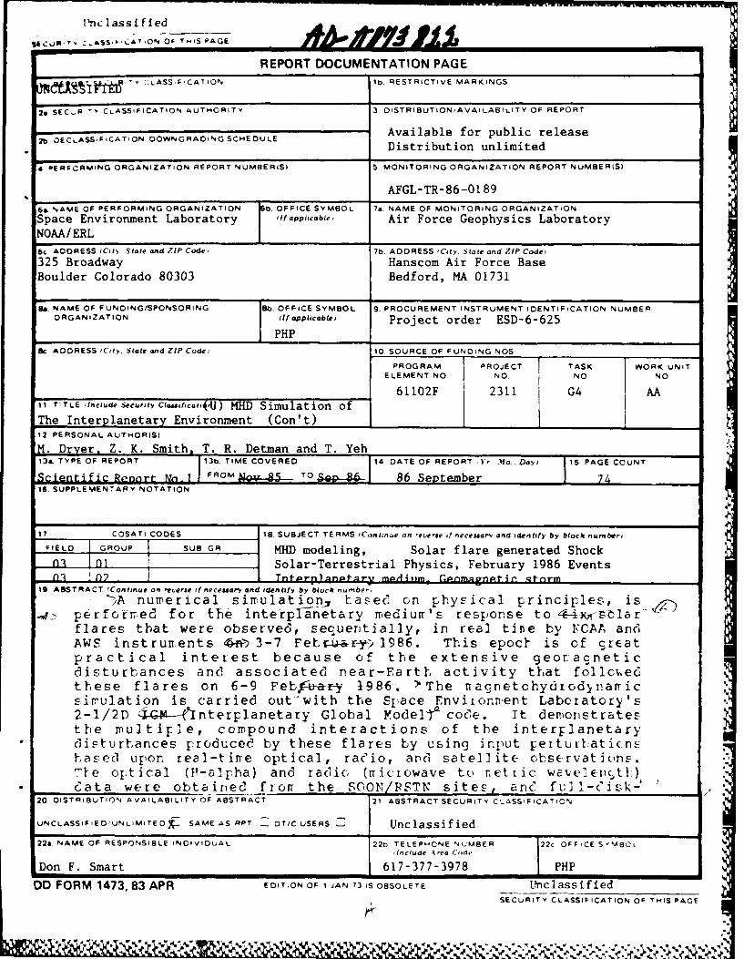
19 ABSTRACT 'Continue on reverse if neceuary and identify by block number,F I -A numperical simulat io n L7 aseC on physical principles, is4-- perfctred for t-he interplianetary irediurr's response to -x 1a
flares that were observed, secquentially, in real tine by N CAA andAWS instrunents '4iv -3-7 Fetr y,,1986. This epoct is of c;rEatpractical interest because of the extensive geor.-acneticdisturbances and associated near-Earth activity that follc;ue6these flares on 6-9 Febf-uaf-y l98i6. >The nagnetohydiocSnamricsirulation is carried out with the Space Envitonnment Laboratory's%2-1/2D 4414,"enterplanetary Global Yodel& 2code. it denlonstratesthe multirle, compound interactions of the interrlanetarydlisturhances [producee by these flares by using irnput Fertutaticnsh-asecl upon real-tirre optical, radio, andt satellite- obsrzrvatfions.-le optical (F-zilpha) and radio, (mricrowave t(, rettic wave'enctl:)6 ata were obtained fiom. the S0'iON/PSTN sites, andf fLu2I-Cdisk-2
20 DISTRIBUTION AVAILABILITY OF ABSTRACT 21 ABSTRACT SECURITY CL.ASSIFICATION
UNCLASSIFtED'UNLiM'ITEDX. SAME AS RPT OTIC USERS CUnclassified22m, NAME OF RESPONSIB3LE INDIVIDUAL 22t) TELEPHCNE N4UMBER 22c OFF'CE S' MBCL
Don F. Smr 1
DO FORM 1473, 83 APR EDITION OF 1 JAN 73 IS OBSOLETE nlsifeSECURITY CLASSIFICATION OF THIS PAGI
Unclassified
SECURITY CLASSIFICATION OF THIS PAGE
Cant of Block 11:
in the Ecliptic Plane During the 3-9 February 1986 Solar and Geomagnetic Activity
Cant of Block 19 (ABSTRACT)
.~integiated X-ray measurements were obtained f romi 0,A4 NOAA/GOES-5and.,i-6 satellites. Examination of the simnulated solar wind output(s ucl, as n'onentumn flux, and cross-magnetospberic tail electricfield.) at Earth's position indicates that the major geomagneticactivity was probably due primlarily/to the second and fifth solarflares in tbe sixfold sequence. C-Predicted-! gecmnagnetic stormsudeen coimmenceirent c4sQ4, times were early by only about c4-ereft
>A,, 3 -4 hours) for the pulses suggested by the consequences of thesecond and sixth. flares. ~
,The 380 hour simulation, whicth required only CO seconds (CPUtime) on the NOAA/NFS CYPEF 855/205, required 8 Lours clock timeon the~ fae e--Eivl-rcfiient ta-roratoryls) APOLLO workstation. 4Thus,it has 71.otential for realtime operational use by a facili y thatnay not, have access to, or funding for, a sul-ercorrputer ) uch asthe 205.
tinc lassi rima
SECURITY CLASSIFICATION OF THIS PAGE
1. INTRODUCTION
Carrington Rotation 1771 of the sun was characterized by a sequence of
twelve solar flares, commencing 3 February and ending 15 February 1986, from
NOAA/SEL/SESC Regions 4711 and 4713. The optical classification ranged from
SF to 3B and the X-ray classification ranged from M1 to X3. Substantial
geomagnetic activity followed the first six flares in this sequence. In the
preceding several solar rotations, geomagnetic activity was minor during the
first phase of each rotation. There was somewhat more significant geomagnetic
activity during the latter phase of each rotation (presumably, because of
recurrent coronal hole activity). The outstanding geomagnetic (etc.)
activity during the earlier half of Rotation 1771 could, for the most part, be
ascribed to the first set of six flares (or subset thereof). Although one
small recurrent coronal hole made its appearance at the east limb in the
beginning of February, the simulation discussed here will not take it into
account. Our present intention is to focus on the six flares only.
The geomagnetic storm of 6-9 February 1986 qualifies as one of the most
intense on record (Allen, 1986). The effects on an extensive set of
multifarious systems are listed in Table I. The probable causes of these
events have been ascribed (G. R. Heckman, private communication, 1986) in
approximate percentages: (1) events caused by geomagnetic storm effects, 75%; 0
(2) events caused by energetic particles, 15%; and (3) events caused directly .... ............
by the X-rays and microwave emission of the solar flares, 10%.
4 i, tA or - - -
CopyINSPE~rE0.s",I .° .

Our primary purpose is to study the multiple interactions of the flare-
generated disturbances without considering latitudinal gradients of the
disturbed parameters. Our procedure, applied to the ecliptic plane, seems
reasonable for this point of the solar cycle (near-minimum) because the solar
flares took place near that plane within the range 20 3-10 0 S latitude. For the
purpose of the present study, the flares will be assumed to have taken place
in the ecliptic plane which is the plane of analysis for the 2-1/2D
dimensional (D) Interplanetary Global Model (MM) code (Wu et al., 1983; Dryer
and Wu, 1982; Gislason et al., 1984i Dryer et al., 1984; Dryer and Smart,
1984; Dryer, 1985; Dryer et al., 1986b; Dryer and Smith, 1986; and Smith et
al., 1986). The 2-1/2D refers to the fluid analysis that considers all
dependent variables, including the three components of the velocity and
interplanetary magnetic field (IMF) vectors, within the two-dimensional
ecliptic plane. We hope to study the present epoch at a later date with our
fully time-dependent 3D IGM code (Han et al., 1986; Dryer et al., 1986a) in
order to examine the latitudinal and heliospheric current sheet effects.
Our secondary purpose is to study the geoeffectiveness implied by using
the time series of the disturbed solar wind plasma parameters to display the
variations of momentum flux and cross-tail electric field. We will show that
certain flare-generated disturbances (specifically those caused by the second
and fifth flares) are most likely to have caused the major momentum flux and
electric field changes at Earth, implying, therefore, the most significant
geomagnetic and ionospheric disturbance& Stated somewhat differently, the
location of the flare relative to Earth is not, necessarily, the determining
2
%. No%'-- %4 4% N % 4 C
- pA

factor in the geomagnetic response. The intervening interplanetary
configuration preceding a given flare's propagating disturbance is an
important factor in the question of geoeffectiveness.
Any physical model must meet the following criteria before it could be
accepted for operational use:
(1) The underlying assumptions should be a reasonable representation of
the physical phenomena for which a simulation is attempted.
(2) The approach should pass proof-of-principle test by examination for
many cases.
(3) Input data should be available and accurate.
(4) Output information should be useful
In the discussion below we outline the assumptions adopted for the IGM
code within the present context. We note several reasons for the choice of
the present example for testing of the proof-of-principle. We have
constrained our input data to quantities that can be inferred or calculated
from what we consider to be significant real-tim observations. We suggest
below that the momentum flux variability of the solar wind at Earth's orbit
and the magnetospheric cross-tail electric field are examples of important
0geoeffective" parameters of interest to an operational model's utility.
3
C - 1 1,1 1 1 '

In Section 2, we discuss the solar activity and some of the near-Earth
system responses during the 3-9 February 1986 epoch. In particular we discuss
the use of the observed data from the input assumptions of the IGM. The
assumed initial state of the solar wind is also outlined. The results of the
simulations are given in Section 3, followed by some concluding remarks in
Section 4.
2. INTERPLANETARY GL(CAL MODEL
Solar Activity. Two active regions made their appearance during Carrington
Rotation 1771 as shown on the H-alpha inferred neutral line chart in Figure 1
(P. S. McIntosh, private communication, 1986). Region SESC 4711, with central
meridian (CM) passage on 5 February 1986, and Region SESC 4713, with CM
passage on 8 February 1986, produced six flares (five of which were in Region
4711) of interest to our study. A small He I 10830Linferred coronal hole was
detected just north and to the east of the latter active region as shown in
Figure 1. The possible effect of one or more high speed streams (cf., Kojima
and Kakinuma, 1986) will not be considered in our study at this time so that
the potential compound effects of the flares themselves could be assessed. We
plan to include simulations of likely high speed streams at a later time.
During the same phases of the four previous solar rotations, there had
been no significant solar flares or erupting prominences, as evidenced by
arrivals of energetic particles and/or geomagnetic activity. Thus, the
"isolatedw character of this sequence of six flares, as listed in Table II,
taken together with the important systems effects referred to in Table I,
4
suggests itself as a useful candidate for one of many tests of the physical
modeling approach suggested in our earlier work.
The events listed in Table II were detected in real time by the NOAA/AWS
system: GOES (full-disk-integrated X-ray flux) satellites (Garcia, 1986), SOON
(H-alpha filtergrams and optical flare classification), and RSTN (radio
bursts). Estimates of the shock velocity derivable from the Type II bursts
were not made at the RSTN sites andhence, were inferred [even in the absence
*of Type II's in the case of Event (i.e., flare) Numbers 3, 4, and 6] for the
purpose of the simulations. These estimates were inferred on a subjective
basis and, hence, cannot be justified on a rigorous basis. Support for this
approach is provided by the statistical study (when Type II bursts we
detected) of the monotonic relationship of peak X-ray flux and interplanetary
shock velocity reported by Pinter and Dryer (1985).
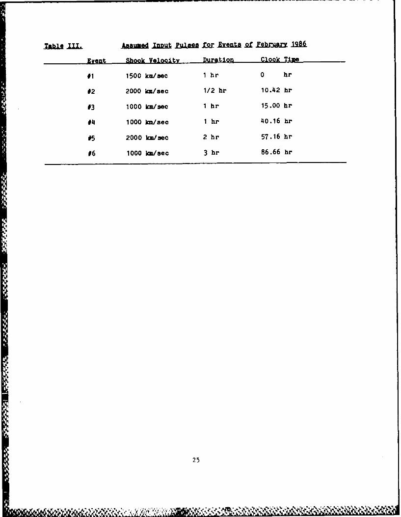
Input Pulse Assumptions for MHD Simulation. We assumed that each event
(flare) produced a coronal shock wave as noted above. The initial shock
velocity, relative to an assumed uniform background solar wind, is given in
Table III for each event. These values are then used to compute the MHD
Rankine-Hugoniot jump conditions at the radial position of 18 Rs (Rs = 1 solar
radius = 6.97 x 10⁵ kin) along each flare's meridian. This position was chosen
because it is a representative point beyond all steady-state critical points
in the solar wind. The steady-state solution is discussed below. We assume
that the shock leaves the flare's vicinity and moves to the inner boundary (18
RS ) of the computational domain (half of the ecliptic plane) at this velocity.
The clock time given in Table III starts (t 0 hr) when the first shock,
5
N :,S .. ~

which we assume to have left the sun at approximately the time of X-ray
maximum of the first flare, arrives at 18 R s. The same assumption is made for
each of the succeeding events as listed in Table III. These shocks, then,
should be considered to be piston driven to, and slightly beyond (as explained
below), this position of 18 Rs. An extensive study of piston driven shocks,
and their subsequent attenuation into blast waves, has been given by Smart and
Shea (1985). The basic ideas (constant velocity propagation followed by a
power law deceleration) included within that empirical study are also
contained within the more detailed simulation in the present paper.
We also assumed a sinusoidal spatial profile of the shock strength over
an 180 included angle centered at the meridian of each flare. This value was
chosen rather arbitrarily in order to provide a representative non-spherical
*extension of the disturbance that emanated from the flare site. Temporally, a
trapezoidal rise and fall for each parameter at each heliolongitudinal
position was assumed for periods of time listed in Table III. This duration
was chosen to be the additional piston driving time as suggested by inspection
of the temporal profiles of X-ray flux measured by the GOES satellites. This
inspection was straight forward in the determination of the moment of initial
rise above background flux but arbitrary in the choice of the time of return
to near-background. A subjective duration, rounded off in units of one-half-
hour, was chosen as a result of this inspection. This characterization of
each flare's contribution of energy, momentum, and mass to the surrounding
corona and solar wind is a crude approximation of what are basically poorly
understood phenomena in solar flare physics. Our goal is to describe large-
scale features in space and time. Hence, we believe that these input
6
"-.0'4 - ." '' '-".', ,, ', " . ' v ' . , ' - ' ' ' ' .' . ' . " , . '-. '--. .. '

assumptions can be considered reasonable representations of the actual
physical phenomena. We found in a very limited test of sensitivity, for
example, that the shock created by Flare 2 arrived at Earth about 5 hours
earlier than the case studied here when the hypothesized piston duration was
increased (Table III) from 1/2 hour to 1 hour and all other parameters were
unchanged. Yet the global structure, to be described below, of IMF and plasma
was not changed in any appreciable way. Nevertheless, it is appropriate to
note that any success in describing large-scale features does not relieve the
modeler of any burden of making the best possible assumptions for input.
Initial Steady State of tIe Interplanetary Medium. We assumed that the
initial state of the interplanetary medium (prior to t = 0) was homogeneous;
i.e., independent of heliolongitude. Moreover, we assumed that the IMF
contained an initial southward component. In the 2-1/2D computational code,
the partial differential equations for the governing physical laws for
conservation of mass, momentum, and energy and Maxwell's equations (Wu et al.,
1983) are written with three independent variables (t, r, *) and eight
dependent variables (Vr, V0 , V, Br, BY BV n, T). The partial derivatives
with respect to helio-colatitude 8 at the equatorial plane are assumed to be
zero. [This restriction has been removed in the full 3D code described by Han
et al., 1986].
The initial steady state is established by first assuming a
representative data set and then allowing the numerical solution of the time-
dependent equations to relax into a steady state solution within an acceptable
tolerance level The sun-centered spherical coordinate system is used with
7
heliocentric radius r increasing outward, the helio-colatitude e increasing
downward from 00 at the northern axis, and the heliolongitude * increasing
from 00 at the east limb as viewed from Earth. The range of spatial variables
in the simulation is from 18 Rs r<232 Rs (1.1 AU), 90 ,and 00 < <
1800.
Table IV includes the initial solar wind plasma and IMF values at both
the inner boundary, (viz., 18 R.), and just within the outer boundary (viz., 1
AU) of the computational domain. The derived parameters: plasma beta 0,
total pressure P, and momentum flux nmV 2 are also listed in the table. The
IMF should be recognized as having a positive (viz., "away") polarity by
virtue of the positive radial and negative azimuthal components as described
in a sun-centered spherical coordinate system. We may consider that the
magnetic flux that leaves the sun in this half-plane returns to it in the
other half-plane of the ecliptic.
3. RESULTS
Global View of the Half-Ecliptic Plane: Figure 2 presents, graphically, the
initial (t = 0 hr) steady-state parameters (Vr, n, T, P, and the unit vector
of the IMF as projected into the ecliptic plane) as summarized in Table IV.
At the upper left corner, the radial velocity is plotted upward in the three-
dimensional graphical presentation of the uniform solar wind in the half-
ecliptic plane as "viewed" by an observer, at r > 1 AU, who "looks" toward the
sun. The velocity Vr is equal to 255 km/sec at the inner boundary of 18 Rs,
which is not seen in this perspective. The east and west limb meridians are,
, 5

respectively, to the left and right of the reader's perspective. The vertical
"cliff" at 1.1 AU is, of course, a graphics artifact but can be used from one
figure to another to assess the scale change that was required by the graphics
software on occasion. In Figure 2, the higher value of Vr = 355 km/sec at 1.0
AU can easily be inferred near the foreground of the symmetrically uniform
solar wind at t = 0 hr. The plot at the lower right corner of Figure 2 shows
the Archimedean spiral of the IMF as viewed from the northern solar pole; this
IMF direction is, of course, indicated by the unit vectors as projected into
the ecliptic plane. The remaining three plots display the proton density,
temperature, and total pressure in a logarithmic scale (base 10). In
succeeding figures, (for 0 < t * . 180.1 hr), the upper right corner (blank in
Figure 2) is used to display the solar wind vector change, Vr, relative to
the initial steady state undisturbed value at each location. The maximum
velocity changc i listed on each of these figures. Each figure (with its
six panels) displays the properties in -5 hour increments. Each spatial tick
mark refers to 0.1 AU per division. Time "zero" (t = 0 hr), as described
earlier, is started when the shock from the first flare reaches 18 Rs; this
time corresponds (approximately) to 2300 UT on 3 February 1986 when converted
to real time. Hence, the reader can anDroximate the simulation's clock time
at t = 0 hr to correspond, roughly, to the start of 4 February 1986. Earth is
located along the vertical axis; the sun is at the origin as viewed from above
the ecliptic plane.
Discussion of Time-Dependent Simulation; The results of the simulated
interplanetary environment during this epoch of solar and geomagnetic activity
are best seen from the perspective of a hypothetical observer who looks down
9

at the half-ecliptic plane from, say, the northern pole of the sun. A number
of interactions will be seen as the evolving disturbances move outwardly from
the solar neighborhood to that of Earth. Formation of forward and reverse
interplanetary shocks will be identified without ambiguity. Shock strength
attenuation of some flare disturbances will be pointed out when one forward
shock propagates into a region that has been accelerated by a preceeding shock
from an earlier flare. We will also observe the effects of a longer-lasting,
piston driven, forward shock as it overtakes and interacts with the reverse
shock from a previous flare. Some of these effects involve the global
distortion of the overtaking shocks. It will be shown that only three flares
from the sequence of six were "geoeffective". Following this sequence of
dispersion, interaction, and distortion of the staccato solar events in this
epoch, the hypothetical observer will note a gradual return to the original,
steady-state parameters discussed earlier.
Figures 3-38 display the simulated response of the interplanetary medium
at intervals of approximately 5 hours, from t = 5.2 hr to t = 180.1 hr.
Identification comments are occasionally made on the figures. Thus, "Flare
1", as indicated on the top left panel of Figure 3, refers to the
interplanetary disturbance caused by the first flare as discussed earlier. No-. _%'
-A' special designation is assigned to the products for interacting shocks
(forward with forward, forward with reverse, etc. as discussed in greater
detail by Smith et al., 1986); instead we chose to continue with the
designation of the stronger interplanetary shock. Thus, for example, the
interplanetary disturbance labeled as Flare 2 in Figures 5-7 is observed to
overtake Flare 1. The latter is then no longer referred to. Instead, we
10
observe the development of the fast reverse MHD shock that follows the fast
forward MHD shock from Flare 2 in Figures 8-10.
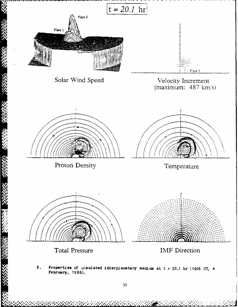
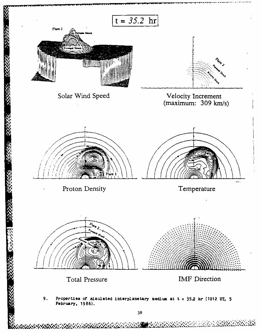
Inspection of the density contours in Figures 8-10 also reveals the more
inconsequential effects of Flare 3 that, nevertheless, must blend in with the
effects of Flare 2. The forward and reverse shocks of the latter are also
labeled in these and subsequent figures. The reverse shocks are most easily
identified by the steepening of the temperature contours closest to the
flare's meridian. An alternative approach, though harder to identify because
of the graphical scale, is the velocity vector plot (upper right corner of
Figures 8-10) which shows that the faster solar wind, produced initially by
the stronger Flare 2, is caused to slow down in the frame of an observer
riding on the reverse shock. Figures 8 and 9, for example, show the location
of Flare 2's reverse shock and the reduction in length of the velocity
increment vectors as one moves outwardly in helioradius.
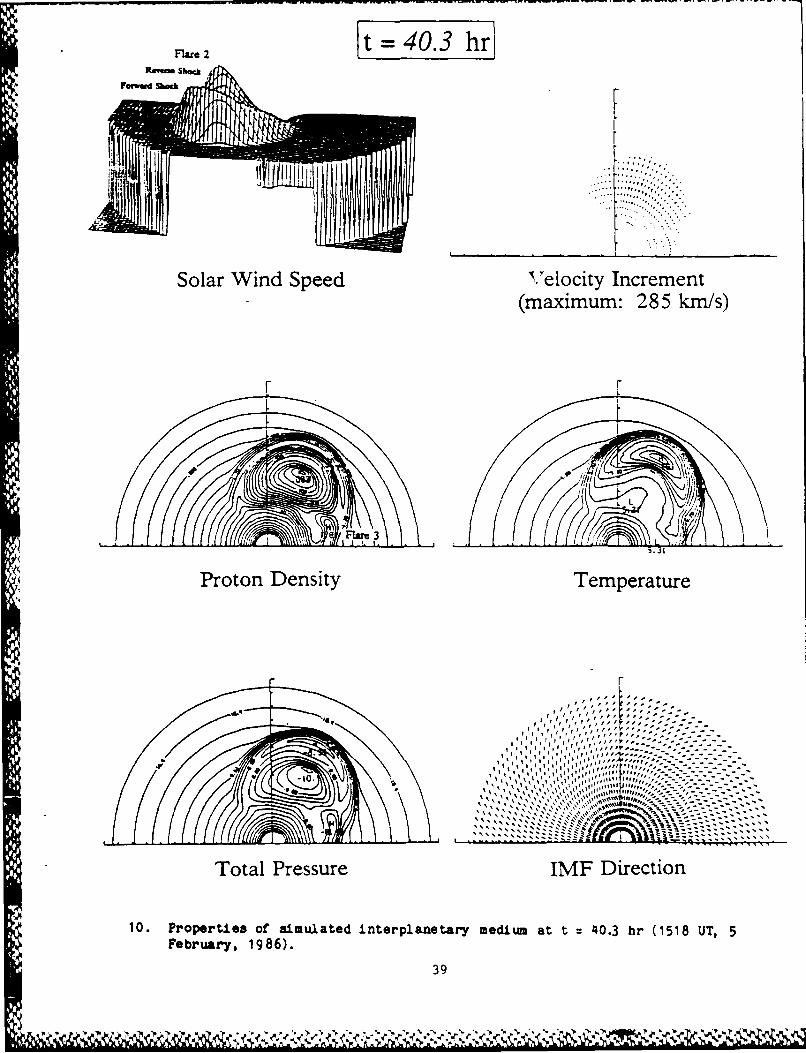
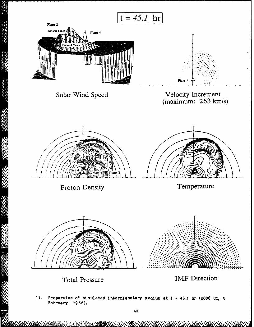
Flare 4 is observed at t = 45.1 hr in Figure 11 near Earth's central
meridian. Flare 3 can still be identified in the contour plots (seen, for
example, in the density ,urves) but cannot be seen from the perspective of the
viewer in the upper left, three-dimensional velocity plot because of the
foreshadowing effects of Flare 2. Distortion of the IMF is clearly seen in
the unit vector presentation of each of these figures. Eventually, Flare 3
can be observed in the velocity plot (Figure 13) as the effects of Flare 2 are
attenuated.
We have also attempted to identify the reverse shock associated with
11
.- P %I

Flare 2 in Figure 13 by reference to the requirement of a shift of polarity
(and increasing magnitude) to the east. This polarity shift is also seen near
the central axis of the forward shock in the lower right panel of Figure 13.
Flare 5, the result of the longer-lasting piston driven shock (simulating
the main features of the flare on 6 February 1986, 0625 UT), is clearly seen
in Figure 14 at t = 60 hr. This disturbance rapidly overtakes and overwhelms
Flare 4 as suggested in Figures 15 and 16. We also observe, in Figures 17-20,
the overtaking of Flare 2's reverse shock by Flare 5's forward shock. The
early stages of Flare 6 are also detected at t = 90 hr in Figure 20 just as
its piston driven phase ends and its blast phase begins.
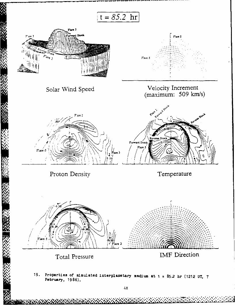
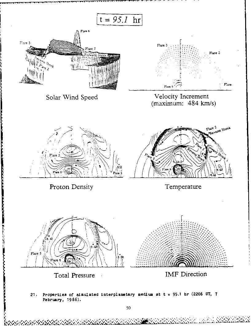
The development of the reverse shock from Flare 5 and the distortion of
its forward shock are seen in Figures 20 and 21. The distortion is
undoubtedly indicated by its interaction with the reverse shock of Flare 2 as
noted above.
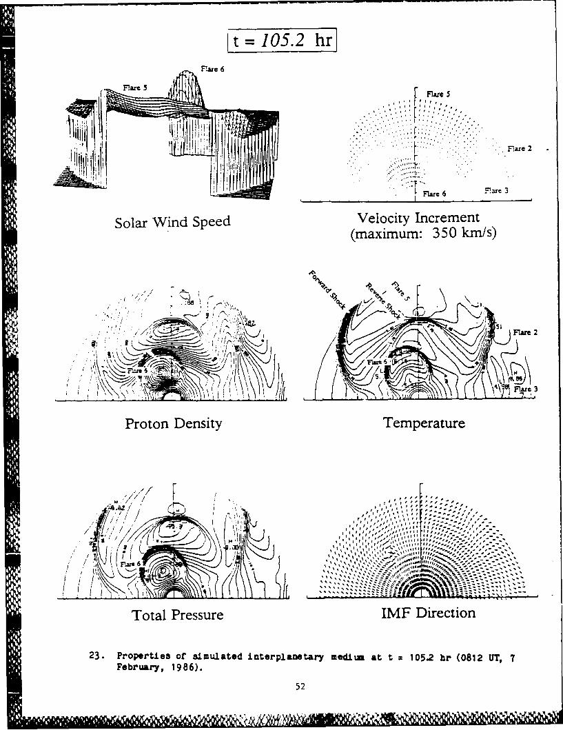
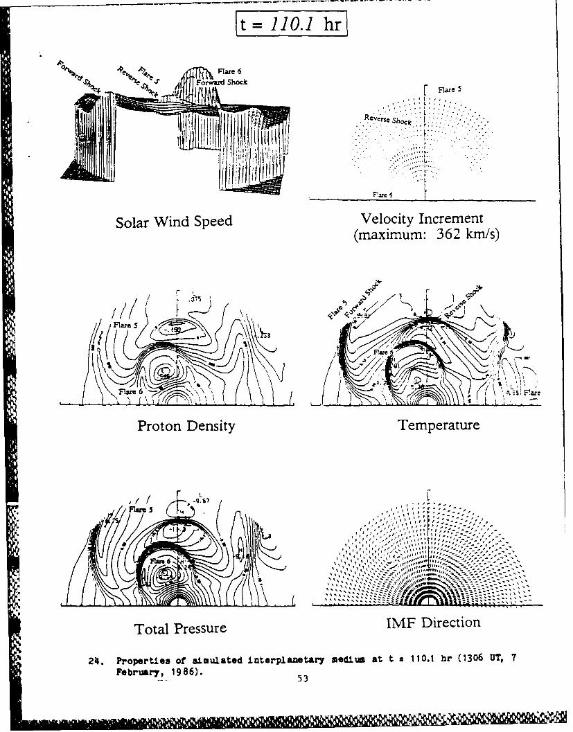
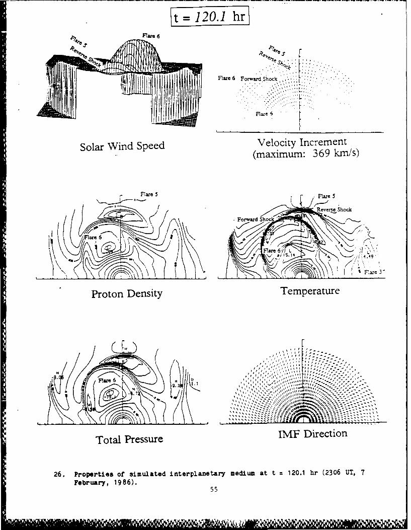
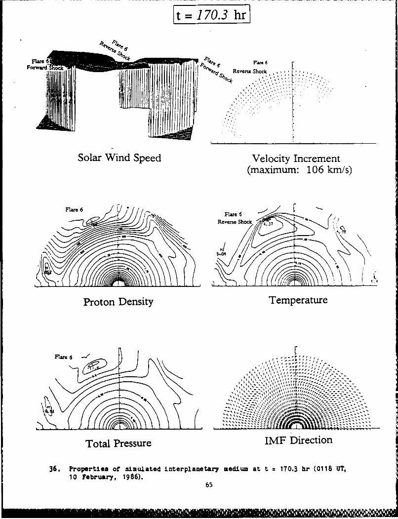
Flare 6, as seen in Figures 22-27, has a similar scenario, namely the
overtaking of the reverse shock of the earlier Flare 5 by the forward shock of
Flare 6. Collision takes place, again in a spatially oblique configuration,
in Figure 27 (t = 125.2 hr), just beyond Earth's position.
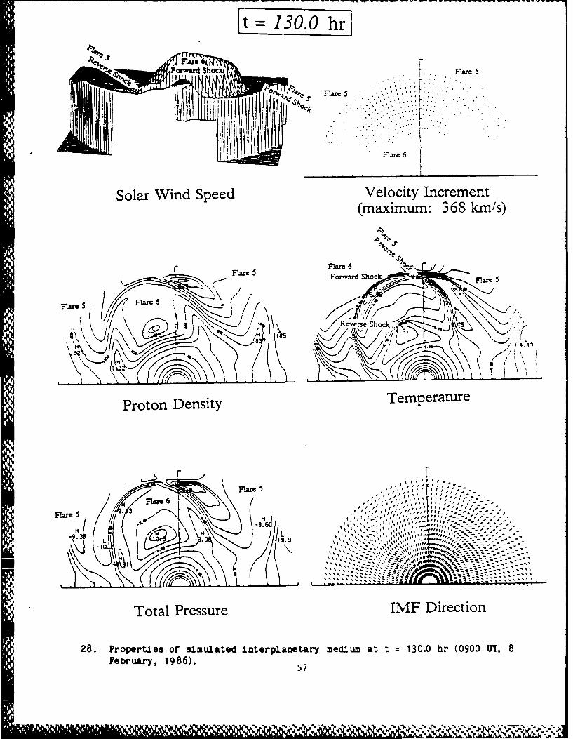
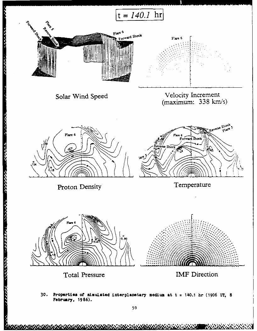
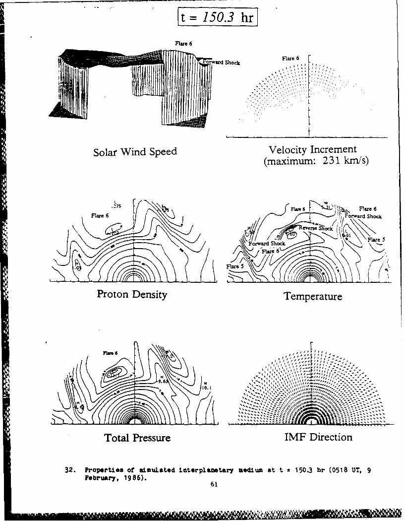
In the remaining figures of this sequence (Figures 27-38), we observe the
dispersion and attenuation of Flare 6. There is a gradual return to the
original, steady-state parameters and Archimedean spiral form of the IMF.
12
TiJLue Series 91 Pla n- IMF at i AU. Our interest for potential
operational interpretations and eventual comparison with observations is
clearly directed to the output at various points in the ecliptic plane.
Observations, when available, from IMP-8 at Earth and the *Halley Armada"
(VEGA 1/2, GIOTTO, SAKIGAKE, SUISEI, and ICE) will obviously be of great
interest in this respect. At this time, we direct attention to six
hypothetical observation points at 1 AU.
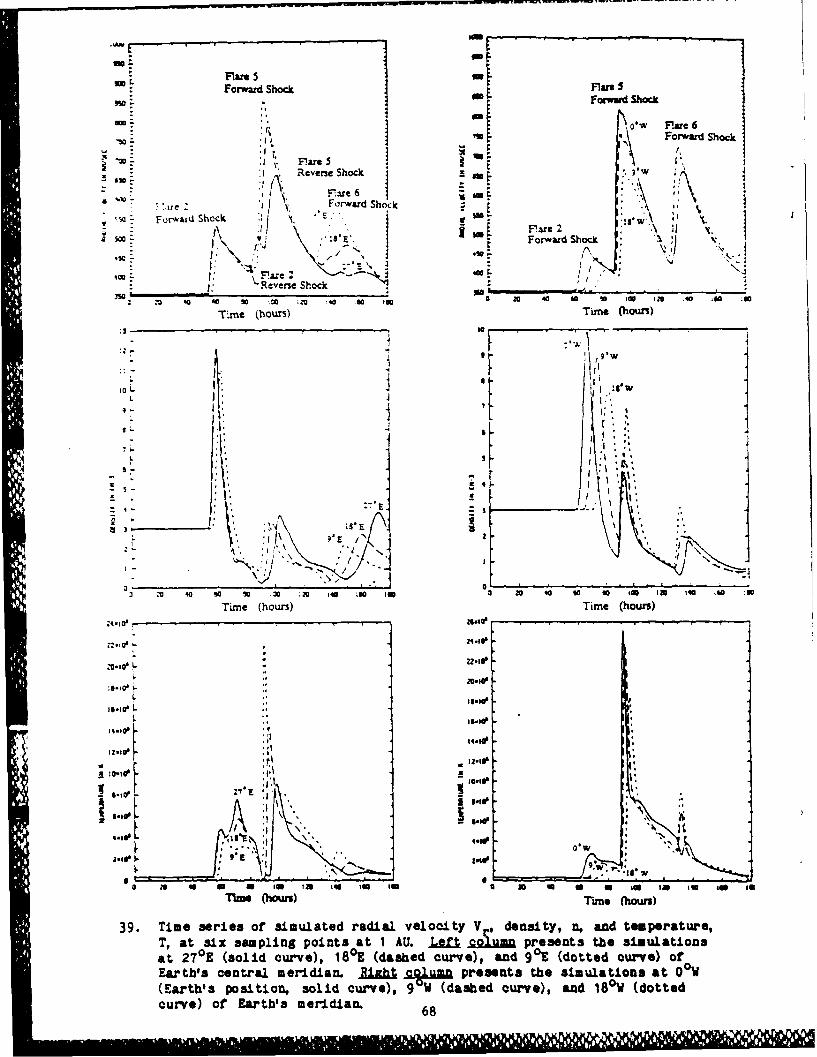
Figure 39 shows the time series of Vr, n, and T at these six positions.
The left column of the figure shows these simulated parameters at three solar
longitudes: 27 0 E, 18 0 E, and 9 0 E of the Earth's meridian. Recall that the
Earth is located along the vertical axis in the previous Figures 2-38. The
right column of panels in Figure 39 refers to three additional solar
longitudes: 0°W (i.e., Earth's location), 9 0 W, and 18°W of Earth's meridian.
Flare 2's forward shock produced jumps that were somewhat larger to the
east of Earth. This was expected because Flare 2 occurred at 21 0 E of Earth's
meridian. There was an effect indicated in the parameters (AV : 100 km/sec)
at t : 85 hr when the stronger portion of Flare 2's reverse shock arrived at
the 27 0 E and 18 0 E positions. As anticipated (see the contours of n, T, and P
in Figures 18, 19, and 20), there was no perceptible change at the 9 0 E
position until Flare 5's forward shock arrived at t = 85 - 90 hr. Arrival of
Flare 5's reverse shock at the three eastern positions is observed best in the
velocity plot, followed shortly by Flare 6's forward shock.
The major disturbances at Earth are indicated (Figure 39, right side,
13
solid curve) to be due to the disturbances associated with the forward shocks
from Flare 2, Flare 5, and Flare 6. The other two positions at 9 0 W and 180 W
experience a delay in response from Flare 2 and Flare 5 but have an earlier
response, compared with that at Earth, from Flare 6.
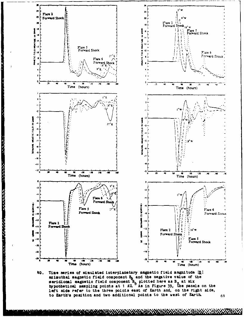
The time series for the magnitude j1I of the IMF is shown in Figure 40
(top panels) for the same six positions. The azimuthal component Bf is shown
in the middle panels, and the meridional component B8 is plotted (with the
appropriate sign change) in the lower panels (labeled as Bz). The latter, Bz,
is customarily used in the solar-ecliptic coordinate system (with the X-axis
pointed to the sun, the Y-axis pointed to the east of the observing position,
and the Z-axis forming the remainder of a right-handed system). This usage is
conventionally used by magnetospheric physicists It is seen that the pre-
existing southward field is compressed by Flare 2 to nearly -20Y followed by
a large-scale rotation moving toward, but never achieving, a northward
polarity. The rotation involves a large-amplitude Alf'ven wave which is then
hit by Flare 5 and the sequence is repeated, albeit at smaller magnitude,
after collision with Flare 6.
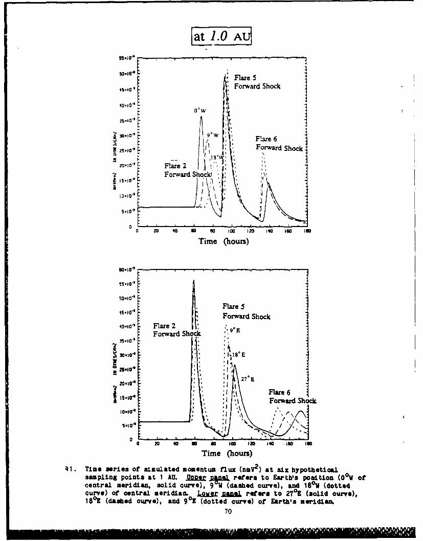
The time series for momentum flux is shown in Figure 41. Flare 5 clearly
is indicated to be the major pulse at Earth (upper panel, solid line).
%Indeed, preliminary information (C. Rufenach, private communication, 1986)
indicates, from GOES 5/6 magnetometer data, that a series of four magnetopause
crossings took place at the geosynchronous (6.6 RE) altitude during the period
* starting with Flare 5's forward shock until that disturbance's decay. The
last two magnetopause crossings (including the one with the longest duration
14
! ' , . , ,"" , ,," .- ' ". "o "'' '""". ." ' """ "',',-"" ," % ' , "4 V 'I" "
between crossings) occurred when, according to the simulation, the momentum
flux was decreasing and, indeed, was even less than that for the original
undisturbed solar wind. This observation, then, serves to caution the modeler
to reconsider the input (such as the possible high speed stream from the
coronal hole[s] mentioned earlier). We also point out that the present
simulation does not have the spatial resolution to reveal physical phenomena
on scales smaller than .105 km because of the grid size used (Ar = 2Rs, Ae =
30, AS = 30). Turbulent fluctuations, then, cannot be simulated in the
present model. It is of interest to note that the storm sudden commencements
implied by the arrival at Earth of the forward shocks associated with Flare 2
and Flare 6 at t - 60 hr and :135 hr (the latter, during the interaction with
Flare 5's reverse shock) correspond fairly well with the actual SSC's observed
on 6 February (1313 UT) and 9 February (1748 UT) 1986. The clock time for the
* actual SSC's would require the simulation to have been at t = 62.2 hr and
138.8 hr, thereby indicating the "predictions" to have been early by about 4
percent.
No actual SSC was detected during the pulse designated here as Flare 5
even though the magnetopause responded as noted above. We speculate that thestrong magnetic activity that started on 6 February 1986 and continued until 9
February 1986 may have obscured a clear SSC signal during this interval. In
fact, the Fredericksburg, Virginia, 3-hr K indices for the most disturbed 24
hours of 8-9 February 1986 were 6, 7, 8, 8, 9, 9, 8, 7 as reported by Allen
(1986) thereby indicating validity to our speculation.
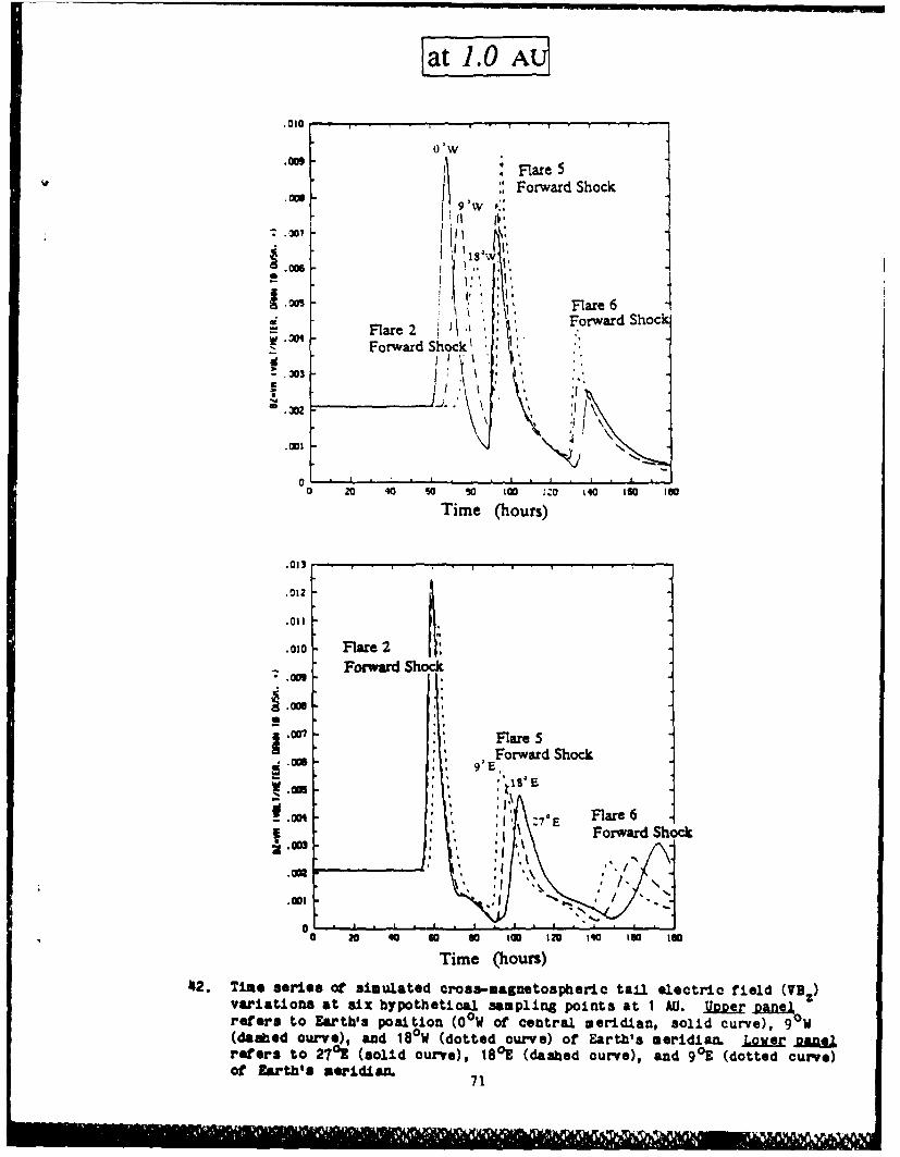
Finally, another "geoeffectiveness" parameter that can be derived from
15
a ; " % " .. " % % " " .% " "" ."" % H " . . - . - - . -

the results of the simulation is the cross-magnetospheric-tail electric field
VBz as shown in Figure 42. The relative magnitudes are again shown at each of
the six 'sampling points" at I AU. VBz exhibits a fourfold increase at the
Earth (top panel, solid line) from 2 mV m" to about 8 mV m- 1 for the first
two pulses (from Flares 2 and 5) and from 0.5 mV m-i to 2.5 mV m- I for the
third pulse (Flare 6). Parenthetically, we note that, had Earth been located
at the 27 0 E position (lower panel, Figure 42, solid line) the simulation
sugg 3sts a sixfold increase in VBz from 2 mV m- 1 to 12.5 mV m- 1 as a result of
the first pulse. Following this latter scenario, the momentum flux (Figure
41, lower panel, solid line) would have increased tenfold from 5 x 10 - 9 to 55
x 10- 9 dyn cm"2 .
We remind the reader that the simulation has used an inertial coordinate
system. Earth has implicitly been assumed to remain at the 1 AU position
along the vertical axis shown in the Figures 2-38. Actually, of course, Earth
moves around the sun at a rate of 1 degree per day. During the period of the
simulation, 4-11 February 1986, a 7 degree movement to the west would have
taken place. We have centered our input pulses at the meridian of each flare
as viewed from Earth (see Table II). We believe that the uncertainty involved
in our assumptions of spatial and temporal values for the consequences of each
flare is more important than the error suggested in Earth's actual location
during this epoch. Nevertheless, some compensation for this movement may be
approximated by interpolation between the additional, hypothetical, "sampling
point" at 90 W and the "Earth's position" at O°W of CM.
16

4. CONCLUDING REMARKS
An MHD, time-dependent, 2-1/2D computer model for the interplanetary
dynamics was used to simulate the disturbances in the interplanetary medium
caused by a series of six flare-induced coronal shocks. This effort was
inspired by the availability of real-time observations during the epoch of 3-
11 February 1986. We do not claim to represent the real, complex, poorly
understood physical phenomena at and near the flare site by anything more than
a crude approximation based on limited observations and their comparison with
theory and earlier modeling efforts. Comparison with actual observations at
Earth was limited in this study to the times of SSC's. These comparisons
between observations and simulations are encouraging. The simulated SSC's
arrived at the Earth 3-4 hours before the actual ones for the second and sixth
flares. Additional comparisons must await the availability of spacecraft data
at various points in space.
Further simulations should be made to test the sensitivity of the output
to changes in the many parameters that must be considered. One such test has
been mentioned: an increase in the pulse duration from 1/2 hr to I hr for
Flare 2 resulted in a shock arrival at Earth about 5 hours earlier than that
shown in the present paper. Other sensitivity tests, such as the omission of
one or more "flare" pulses, should be conducted.
In addition we plan to incorporate the simulation of one or two coronal
hole streams in addition to the present use of six "flare" pulses.
17

The February 1986 epoch has been an ideal period for a study of this kind
because it took place at solar minimum in the absence of any other significant
solar activity. We suggest that much more insight and understanding may be
gained by such a study despite our imperfect knowledge from limited
observations and interpretations. We do believe, however, that a study of a
more complex solar atmosphere that produces an equally complex heliospheric
structure cannot be ignored. Heliospheric current sheets and three-
dimensional effects must be considered in the future so that we can widen our
ability to simulate flare events at higher latitudes, eruptive prominences,
shearing of photospheric and cornal magnetic topologies, and irregularly
shaped high-speed coronal hole stream& These forms of solar activity should
be simulated in various ways, taken both singly and in combination.
In conclusion, we have demonstrated the usefulness of the NOAA/SEL 2-1/2)
Interplanetary Global Model (IGM) to study compound events of important
geophysical interest. Of particular interest is the demonstration of complex
interactions among disturbances from multiple, staccato flares. The study
suggests that the researcher and forecaster can make more meaningful
-v4 assessments of cause and effect in more complicated case&
The computer code required only 100 seconds (CPU time) on the CYBER
855/205 computer for a 180-hour simulation of one-half of the ecliptic plane
covering a radius of 1.1 AU. The same run could be made in 8 hours on the SEL
APOLLO workstation; thus, real-time use in an operational forecasting mode is
possible for a facility that may have neither funding nor access to a
supercomputer such as the CYBER 205. More importantly, simulations of the
.9,4
l '
type discussed here require further testing via comparisons with multi-
spacecraft data sets before operational application is undertaken.
ACKNOWLEDGMENTS
This work has been supported in part by Air Force Geophysics Laboratory
Order No. ESD-6-625. We are grateful for discussions, comments, and
suggestions from J. H. Allen, P. Bornmann, H. Garcia, S. M. Han, G. R.
Heckman, H. Leinbach, P. S. McIntosh, L. Murdock, C. Rufenach, M. A. Shea, D.
F. Smart, T. Speiser, M. D. Szymanowski and S. T. Wu. We also thank T.
Jacobwith for his efficient and rapid preparation of the manuscript.
19

REFEREN4CES
Allen, J. H., Major magnetic storm effects noted, EOS, §1., 537, 1986.
Dryer, M., Interplanetary evolution of solar flare-generated disturbances and
their potential for producing magnetospheric activ~.ty, in Pre in" 2
.Launn Workshoo 9_ Solar Pysics .A InterRlanetary 113aye§Jl Phenomen
(C. de Jager and B. Chen, Eds.), Science Press, Beijing, China, pp. 94i3-
954, 1985.
Dryer, M., and D. F. Smart, Dynamical models of coronal transients and
interplanetary disturbances, _Ady1. Sp Re&,. AM7, 291-301, 198'4.
Dryer, M., and Z. K. Smith, MHD simulation of multiple interplanetary
disturbances during STIP Interval VII (August, 1979), in froggeM..@ .of
the Si~ir Maximum Analyses Symposium (V. E. Stepanov and V. N. Obridko,
Eds.), VNU Science Press, Utrecht, in press, 1986.
Dryer, M., S. T. Wu, and S. M. Han, Three-dimensional, time-dependent, MHD
model of a solar flare-generated interplanetary shock wave, in The Sun
and the Heliosohere 1Ag Three Dimensione4 (R. G. Marsden, Ed.), D. Reidel
Publ. Co., Dordrecht, PP. 135-140, 1986a.
20
Dryer, M., Z. K. Smith, S. T. Wu, S. M. Han, and T. Yeh, MHD simulation of
the 'Geoeffectiveness" of interplanetary disturbances, in Solar Wind-
MaznetosDhere goupling (Y. Kamide and J. A. Slavin, Eds.), Terra
Scientific PubL Co., Tokyo, in press, 1986b.
Dryer, M., and S. T. Wu, Magnetohydrodynamic modelling of interplanetary
disturbances between the sun and earth, Air Force Geophysics Laboratory
Report AFGL-TR-82-0396, 21 December, 1982. ADA130115
Dryer, M., and D. F. Smart, Dynamical models of coronal transients and
interplanetary disturbances, _Ad. Soace IM i(7), 291-301, 1984.
Dryer, M., S. T. Wu, G. Gislason, S. M. Han, Z. K. Smith, J. F. Wang, D. F.
Smart, and M. A. Shea, Magnetohydrodynamic modelling of interplanetary
disturbances between the sun and earth, AStroh. ac Sci. 1, 187-
208, 1984.
Garcia, H. A., Solar flares and the intense geomagnetic storm of Feb. 1986
(abstract), Bull, Amer. Astronom. 1Soc. _U(2), 699-700, 1986.
Gislason, G., M. Dryer, Z. K. Smith, S. T. Wu, and S. M. Han, Interplanetary
disturbances produced by a simulated solar flare and equatorially-
fluctuating heliospheric current sheet, Astroghys. Space §9 149-
161, 1984.
21

Han, S. M., S. T. Wu, and M. Dryer, A transient, three-dimensional MHD model
for numerical simulation of interplanetary disturbances, in STIP
Symosium 9C Retrospective Intervals (M. A. Shea and D. F. Smart, Eds.),
Book Crafters PubL Co., Chelsea, Michigan, in press, 1986.
Kojima, M., and T. Kakinuma, Three-station observations of interplanetary
scintillation at 327 MHz - IL Evolution of two-dimensional solar wind
structure during 1983 to 1985, Proc. Res. Inst. Atmos. (Nagoya
University), 33, 1, 1986.
Pinter, S., and M. Dryer, The influence of the energy emitted by solar flare
X-ray bursts on the propagation of their associated interplanetary shock
waves, Astrophys. Space .cL, 116, 51-60, 1985.
Smart, D. F., and M. A Shea, A simplified model for timing the arrival of
solar flare-initiated shocks, . Geophys. Res. 9, 183-190, 1985.
Smith, Z. K., M. Dryer, and S. M. Han, Interplanetary shock collisions:
forward with reverse shocks, AstroDhy. Spac Sci.. j119, 337-344, 1986.
Wu, S. T., M. Dryer, and S. M. Han, Non-planar MHD model for solar flare-
generated disturbances in the heliospheric equatorial plane, Solar Pys,
D4, 395-418, 1983.
22
~ ~ ~ z....*
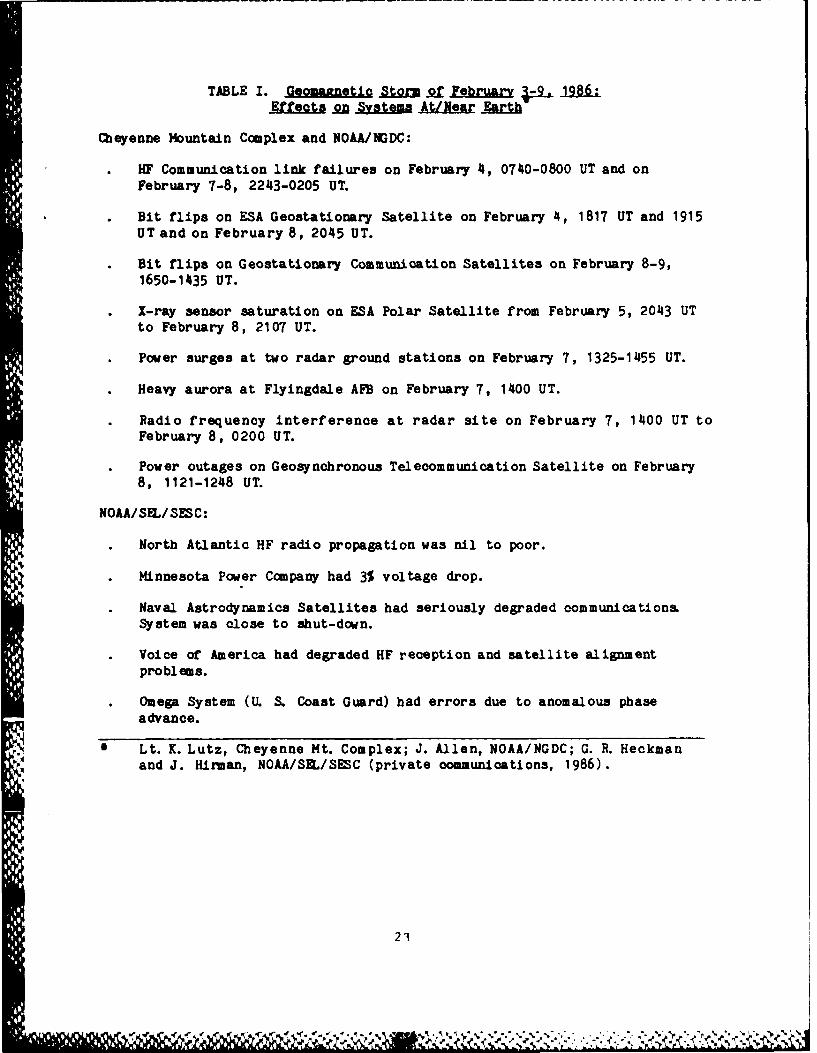
TABLE I. .Qnoanei&,So -Q eru~~ary ki 1 . 12A§-,.Effects _nU Un At/Near Earth
Cheyenne Mountain Complex and NOAA/NGDC:
. HF Communication link failures on February 4, 0740-0800 UT and onFebruary 7-8, 2243-0205 UT.
. Bit flips on ESA Geostationary Satellite on February 4, 1817 UT and 1915UT and on February 8, 2045 UT.
* Bit flips on Geostationary Communication Satellites on February 8-9,1650-1435 UT.
- X-ray sensor saturation on ESA Polar Satellite from February 5, 2043 UT
to February 8, 2107 UT.
Power surges at two radar ground stations on February 7, 1325-1455 UT.
* Heavy aurora at Flyingdale AFB on February 7, 1400 UT.
Radio frequency interference at radar site on February 7, 1400 UT toFebruary 8, 0200 UT.
Power outages on Geosynchronous Telecommunication Satellite on February
8, 1121-1248 UT.
NOAA/SEL/ SESC:
North Atlantic HF radio propagation was nil to poor.
Minnesota Power Company had 3% voltage drop.
Naval Astrodynamics Satellites had seriously degraded communications.System was close to shut-down.
Voice of America had degraded HF reception and satellite alignmentproblems.
Omega System (U. S. Coast Guard) had errors due to anomalous phase
advance.
Lt. K. Lutz, Cheyenne Mt. Complex; J. Allen, NOAA/NGDC; G. R. Heckmanand J. Hirman, NOAA/SE/SESC (private communications, 1986).
21
, " , . .,/ +.,,, .,,. .- - -.-. + -.....- ,. > ' ' N ,
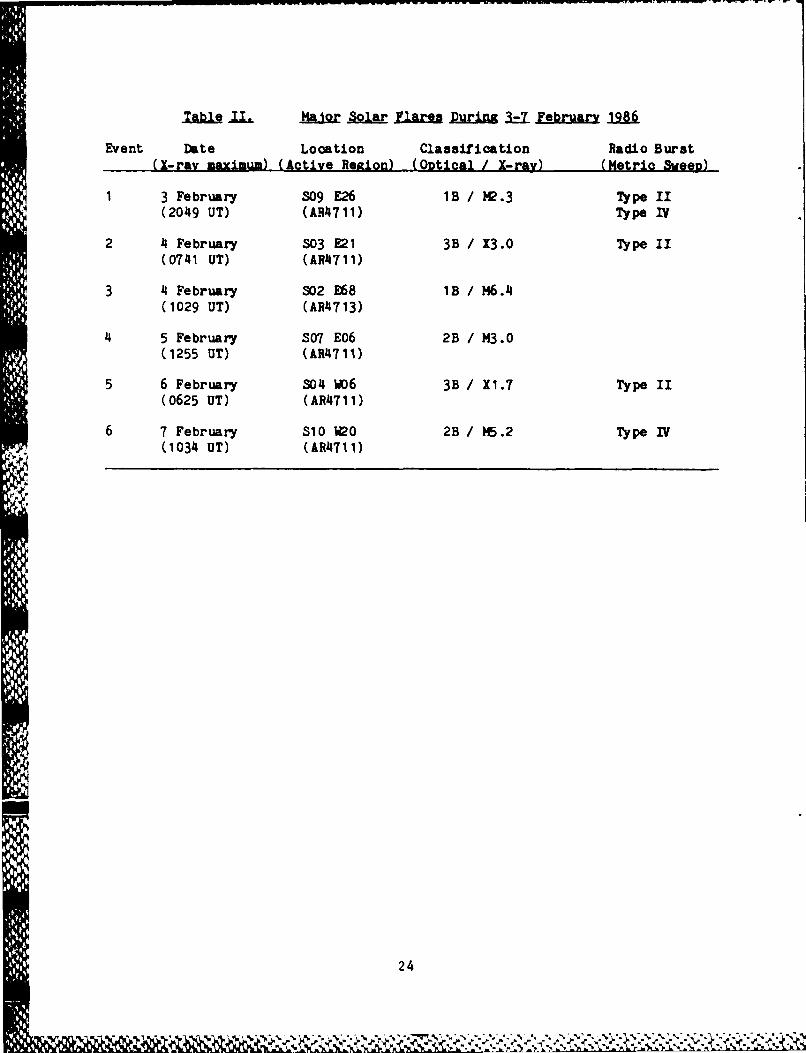
table iL ,i. ,.lar Flres Duri -3- e 1.a I
Event Date Location Classifioation Radio Burst(X-ray maximum) (Active Region) (Ontical / X-ray) (Metric Sweep)
1 3 February S09 E26 1B / M2.3 Type II(2049 UT) (AR4711) Type IV
2 4 February 803 E21 3B / X3.0 Type II(0741 UT) (AR4711)
3 4 February S02 E68 1B / M6.4(1029 UT) (AR4713)
4 5 February S07 E06 2B / M3.0(1255 UT) (AR711)
5 6 February S04 W06 3B / Xl.7 Type II(0625 UT) (AR4711)
6 7 February S10 W20 2B / M5.2 Type IV(1034 UT) (AR4711)
24
IL~.-.
Tab~ l L iAnmes1 Input PHIA2 S Evnsf FeruaI3 191k
Event Shook Velocity Duration Clock Time
#11500 km/sec 1 hr 0 hr
#2 2000 km/sec 1/2 hr 10.4~2 hr
#3 1000 km/sec 1 hr 15.00 hr
#41 1000 km/sec 1 hr 4~0.16 hr
#5 2000 km/sec 2 hr 57.16 hr
#6 1000 km/sec 3 hr 86.66 hr
25

~~TableV Initial St dy--State SolarWd
Parameter I 18 Ra 1 AU
---------------------------Vr (ik me -1 ) I 250. 355.IVe 0.2 0.01
VIv1.0 1 0.35
-- I-----------------------Br (gamma) 1 300. 2.1
IIBe 1 100. 6.0
BI
B, -30. -2.0
n (t-3 ----------- ----------------n (o. 3 ) I 600. 3.0
* ~IIT (°K) 1 1.06 x 10⁶l 3.1 x 10
I I0( 167rnkT/B 2 ) 0.43 1 0.15
P(2nkT + /81) 5.8 x 10-T, 2.0 x 10- 1 0(dyn am-) I -
mV2 (dyn C -2 ) I 6.3 x 10-71 6.3 x 10. 9
---------------------------------- ----------------
26
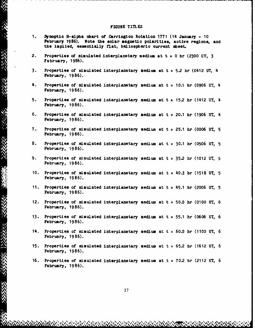
FIGURE TITLES
1. Synoptic H-alpha chart of Carrington Rotation 1771 (114 January - 10February 1986). Note the solar magnetic polarities, active regions, andthe implied, essentially flat, heliospheric current sheet.
2. Properties of simulated interplanetary medium at t = 0 hr (2300 UT, 3February, 1986).
3. Properties of simulated interplanetary medium at t - 5.2 hr (0112 UT, IIFebruary, 1986).
14. Properties of simulated interplanetary medium at t - 10.1 hr (0906 UT, 41February, 1986).
5. Properties of simulated interplanetary medium at t 15.2 hr (1112 UT, 41February, 1986).
6. Properties of simulated interplanetary medium at t 20.1 hr (1906 UT, 41February, 1986).
7. Properties of simulated interplanetary medium at t = 25.1 hr (0006 UT, 5February, 1986).
8. Properties of simulated interplanetary medium at t = 30.1 hr (0506 UT, 5February, 1986).
9. Properties of simulated interplanetary medium at t = 35.2 hr (1012 UT, 5February, 1986).
10. Properties of simulated interplanetary medium at t = 40.3 hr (1518 UT, 5February, 1986).
11. Properties of simulated interplanetary medium at t = 45.1 hr (2006 UT, 5February, 1986).
12. Properties of simulated interplanetary medium at t = 50.0 hr (0100 UT, 6February, 1986).
13. Properties of simulated interplanetary medium at t = 55.1 hr (0606 UT, 6February, 1986).
14. Properties of simulated interplanetary medium at t = 60.0 hr (1100 UT, 6February, 1986).
15. Properties of simulated interplanetary medium at t = 65.2 hr (1612 UT, 6February, 1986).
16. Properties of simulated interplanetary medium at t = 70.2 hr (2112 UT, 6February, 1986).
27
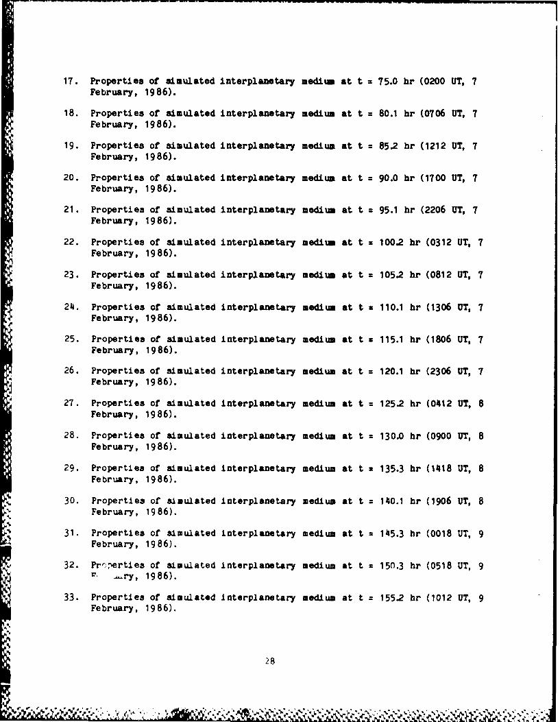
17. Properties of simulated interplanetary medium at t = 75.0 hr (0200 UT, 7February, 1986).
18. Properties of simulated interplanetary medium at t = 80.1 hr (0706 UT, 7February, 1986).
19. Properties of simulated interplanetary medium at t = 85.2 hr (1212 UT, 7February, 1986).
20. Properties of simulated interplanetary medium at t = 90.0 hr (1700 UT, 7February, 1986).
21. Properties of simulated interplanetary medium at t = 95.1 hr (2206 UT, 7February, 1986).
22. Properties of simulated interplanetary medium at t z 100.2 hr (0312 UT, 7February, 1986).
23. Properties of simulated interplanetary medium at t = 105.2 hr (0812 UT, 7February, 1986).
24. Properties of simulated interplanetary medium at t z 110.1 hr (1306 UT, 7February, 1986).
25. Properties of simulated interplanetary medium at t c 115.1 hr (1806 UT, 7February, 1986).
26. Properties of simulated interplanetary medium at t = 120.1 hr (2306 UT, 7February, 1986).
27. Properties of simulated interplanetary medium at t = 125.2 hr (0412 UT, 8February, 1986).
28. Properties of simulated interplanetary medium at t = 130.0 hr (0900 UT, 8February, 1986).
29. Properties of simulated interplanetary medium at t a 135.3 hr (1418 UT, 8February, 1986).
30. Properties of simulated interplanetary medium at t 2 140.1 hr (1906 UT, 8February, 1986).
31. Properties of simulated interplanetary medium at t = 145.3 hr (0018 UT, 9February, 1986).
32. Pr',2erties of simulated interplanetary medium at t c 150.3 hr (0518 UT, 9r .- ry, 1986).
33. Properties of simulated interplanetary edium at t - 155.2 hr (1012 UT, 9February, 1986).
28

34. Properties of simulated interplanetary medium at t = 160.1 hr (1506 UT, 9February, 1986).
35. Properties of simulated interplanetary medium at t = 165.3 hr (2018 UT, 9February, 1986).
36. Properties of simulated interplanetary medium at t = 170.3 hr (0118 UT,10 February, 1986).
37. Properties of simulated interplanetary medium at t = 175.1 hr (0606 UT,10 February, 1986).
38. Properties of simulated interplanetary medium at t = 180.1 hr (1106 UT,10 February, 1986).
39. Time series of simulated radial velocity V , density, n, and temperature,T, at six sampling points at 1 AU. JLf presents the simulationsat 27 0 E (solid curve), 180 E (dashed curve), and 90 E (dotted curve) ofEarth's central meridian. Iiht ag presents the simulations at 0 W(Earth's position, solid curve), 9 W (dashed curve), and 18°W (dottedcurve) of Earth's meridian.
40. Time series of simulated interplanetary magnetic field magnitude Ijazimuthal magnetic field component N and the negative value of themeridioal magnetic field component Be plotted here as B at sixhypothetical sampling points at 1 AU. As in Figure 39, the panels on theleft side refer to the three points east of Earth and, on the right side,to Earth's position and two additional points to the west of Earth.
41. Time series of simulated momentum flux (nmV 2 ) at six hypotheticalsampling points at 1 AU. UJer i refers to Earth's position (0°W ofcentral meridian, solid curve), 9 W (dashed curve), and 18°W (dottedcurve) of central meridian. Low panel refers to 27 0E (solid curve),180 E (dashed curve), and 9 0E (dotted curve) of Earth's meridian
42. Time series of simulated cross-magnetospheric tail electric field (VBZ)variations at six hypothetical sampling points at 1 AU. Upper ennorefers to Earth's position (0°W of central meridian, solid curve), 90 W(dashed curve), and 180 W (dotted curve) of Earth's meridian. Lower panelrefers to 270 E (solid curve), 18°E (dashed curve), and 90 E (dotted curve)of Earth's meridian.
V.
29
i'

www w-31F-
. -W 19
* -7-
4- 0IALjob 0
411
0 to -
7 i Val
z- -0
04
IT I
j If-
S-1
30I-

Solar Wind Speed
Proton Density Temperature
IMF~F Diecio
2.F' Prprte Of' 31Muate inepantr meiu att=0h 20 T
February, 1986).
31 FF'FFF---

Solar Wind Speed Velocity Increment(maximum: 357 kmls)
Proton Density Temperature
'all
A, b-
Total~~- Presur IM-ieto
3. Properte3 Of ai-------intep-anetary-edium-at----5.2--r-0412-UT,-
sc a February, 1986).* ''~ --32

It =10. 1hr
Solar Wind Speed Velocity Increment
(maximumn: 258 km/s)
Proton Density Temperature
Tota PresureIMFDirection
4I. Properties of siul~ated interplanetary medium at t 10.1 hr (0906 UT, 4* February, 1986).
33
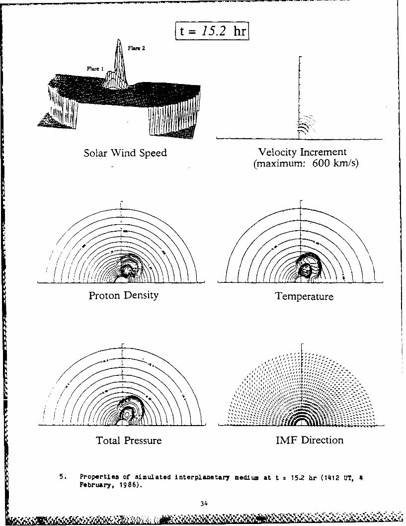
Solar Wind Speed Velocity Increment(maximum: 600 kmls)
//L
Proton Density Temperature
lb'
Tota Pressur IM Diretio
5. roprtis f smulte inerpanear meiumat t 15- hr(42-T
Fe r ay 1986).,, ~'A- --
34'' 9991 '
t20.1 hr
F . Fare-'
Solar Wind Speed Velocity Increment(maximum: 487 kmi's)
Proton Density Temperature
. . . . . . . . . . . . . . . .. ..... .. . . .
February, 1986)
35 S ~ '''"~. -

t25.1 hrl
Solar Wind Speed Velocity Increment(maximum: 400 km/s)
PrtnDest Tepratr
Proton DresitTmpraur
Febrar. 1986). 3

It= 30.1 hr]
*ev
Solar Wind Speed Velocity increment
(maximum- 331 kmls)
Proton Density Temperature
Total Pressure IMF Direction
8. Properties of simulated interplanetary medium at t =30.1 hr (0506 UT, 5February, 1986).
37
t=352hr
Rmn, It o
Solar Wind Speed Velocity Increment(maximum. 309 kmls)
/r
4 ~~~ i 7 / 'IJ '
Proton Density Temperature
r-
. I . .. .. . . .. .-- - - .
Toa Prssr IM D~,iection-- --
9. Poperies f smulaed iterlaneary edim att a 5.2hr (012 T,Febrary 1986).-
38%
Flue 2. t= 40.3 hrl
Solar Wind Speed X.:elocity Increment(maximum: 285 kmls)
Flue 3
Proton Density Temperature
~~X---
Total Prssr IM Diecio
10 Poete ofamltditrlntr mdiu at t =I 403h 11 -T
Fe ra y 1986).,'I~,I,,t:,,a,''--- - -
39 ~It~jll
t_=45.1 hrlFlare 2
Fare 4 '
Solar Wind Speed Velocity Increment(maximum: 263 kmls)
F/il 4 U y" are
Proton Density Temperature
. VNAN-- -
Total Pressure IMIF Direction
11. Properties of simulated interplanetary medium at t a '45.1 hr (2006 UT, 5February, 1986).
4

Mlarc 2 =50.0 hrl
L
Fare 4
Solar Wind Speed Velocity Increment(maximum: 234 km~s)
44
Proton Density Temperature
Ferury 1986).
-5- ' ZS~-'-

Rgvem Shoc 55.1 hr]
1 fit! ff
F'~Ame3
Solar Wind Speed Velocity Increment(maximum: 208 kmls)
Proton Density Temperature
I Flu 3
Total ressue IMFDirecion.......
13.~~ Prprte of siuae inepaeaymdu t 51h 00 TFebruary, 1986)
I,,,42

Flue 5
Solar Wind Speed Velocity Increment(maximum: 1290 kmls)
Proton Density Temperature
Feray 1986).
43,I'4 "

Flim 5
-. r
Solar Wind Speed Velocity Increment
(maximum: 784 kmls)
S-U e
_l. arer 4/,7
,V' III( L .
IProton Density Temperature
71/7
Total Pressure IMF Direction
15. Properties of simulated interplanetary medium at t =65.2 hr (1612 UT, 6February, 1986).
44

Flare 5 El (
ofFware
F~Fare 5
Solar Wind Speed Velocity Increment(maximum: 582' kmls)
''re 3 Far:r'5
Proton Density Temperature
Flu Z,,
Flam 5r-
3
ToalPrssr IF Dieto
16. Proertiesof simlated nterplaetary edium t t 702 hr (212 UT,
* ~~F br a y 1986) 45 *~ * FF~F~ S~ ~Jt.

t= 75.0 hrl
Flare 5
SoavrzWid Sped eoct Icemn
(maximum: 497 kmls)
744
Proton Density Temperature
aus 3
Ferury 196) 46f',Pt - -

it= 80.1 hr]Flae 5
Flare 31 j~owr Shock
SolarWind peedVelocity Increment
Solr indSped(maximum: 479 km/s)
a Flare2
/1 - ?
FareII 3
Proton Density Temperature
FFlare
TotalPressre IF Dirctio
18.~~~~~~~~~~~~~~ Prprino --ae itrlntr eima t=8. r(70 T
Fe rury 1986). -S
"' L'.~ 5 ~.'~K~ -47
Fu43 o. Iar S o [ ae 2
1'k
SolarWind peedVelocity IncrementSolarWind peed(maximum: 5 09 kmls)
Reen Soc
Flare -5 L
/I ,-; I ,
Elite-S ~ lit.
~e 3
ProtnPesueIFDieto
*t48

t = 90.0 hrl
Flare 3Flarx~~Fcnvard Shock p are." =
Flare 5
Solar Wind Speed Velocity Increment(maximum: 734 kmis)
7een " 7, ,
, . C ~ ;-d c-;r-_,
I"- "Flar 5i Flar 5N~
arej M/ Fare________________6__
Proton Density Temperature
Ax
rr
I0
,,,, , , ,,,, ,:;: -- ,
.. . . .... ..A:
.,sit
-,' F Flare 3 ,, ".. . . " ",
Total Pressure IMF Direction
!20. Properties of simulated interplanetary medium at t = 90.0 hr (1700 UT, 7February, 1986). 4
S I . . . . . , .. . ,, F l - F - F. . - • w , , , ,' , ' - .
,,, . . . . .. ,€, ,<, '. .%. .. • ., , -,, . ,. . . , ' . , # , F- FF,, . . ," . , ' , , .
,/ ,",,t , ", . ' . , . ," w , . / , ., . . ' " ' - , ., • . ,.A.'• , , ' %
it-95.1 hrI
FlareS , ,5
@, ., , !..
F=e 5 Pare
Solar Wind Speed Velocity Increment(maximum: 484 km/s)
Proton Density Temperature
12(
a.
Flare3 _ _ _ _ _ _ _ _ _ _ _ _ _ _
Total Pressure IMF Direction
21. Properties of simulated interplanetary mediume at t =95.1 hr (2206 UT, 7February, 1986).
50
. .- - .- " " " . .- - ' -- -

t =100.2 hrl
FFlare 5
Rare
Rare 6 Pare 3
Solar Wind Speed Velocity increment(maximum: 426 km/s)
~~owFlare 5 orwlSe Shoce L ck
_____ard~o~k
',..RaiR
Proton~~~ar Dest2eprtr
rt A.VS
FlaeZ~lar 6 . ;ji
Trotal Prensite IemperDireo
22. Propert1e3 Of simulated interplanetary medium at t =100.2 hr (0312 UT, 7
February, 1986). 51
t =105.2 hrI
Flare 6
• i I :- .:Y ..,' '" !~""... , .. ":i:.. .::"i:.. . .... ,
- Flare 6 Flare 3
Solar Wind Speed Velocity Increment(maximum: 350 km/s)
0%
______ ft.' F~are
Proton Density Temperature
, , -1.February, 19 86)
52,, ',,,,,,, ; s -- - - -I II Ii i sil - r / ,/ I K IIIII i,,I , I. i IIIlt
/1 ,,, ,,,,.--- <.,,. , - .- - . .-.
Total Pressure IMF Direction
23. Properties ot simulated interplanetary medii am t t :105.2 hr (0812 UiT, 7February, 1986).
52
AO4 e Flare 6% Forward Shock [Flare5
Sola Wid _________ eee Shock.
Soa idSpeed VelocityInrm t(maximum: 362 kmls)
roto Dest Tempeatur
7 71,
Prto Dest Teprature
/9 L1 67--Flare
---- ,
RAN'~~i:-- 4-
4,~
Total Pressure IMF Direction
241. Properties of simulated interplanetary MedauM at t 2110.1 hr (1306 UT# 7February, 1986). 53

~t115.1 _hrl
Flaraee6
Revere S ock.
SSh~ock"
Flare 6. .
Solar Wind Speed Velocity Increment(maximum: 368 krn/s)
L
Proton Density Temperature
Flare~ 5 L81
Total Pressure IM Drci
25. ~ ~ ~ ~ ~ ~ ~ ~ ~ ~ ~ ~ ~ ~ ~ ~ -Prprte ofsmltditrlai-r eima 151h 10 T
Feray 1986)
54, I '.- . 9..
Pare 12. r
~II iiFlare 6 Forward Shock
I 'Flar e 5
Solar Wind Speed Velocity Increment(maximum: 369 k-m/s)
Fae5Flare5
Flare 6>
Proton Density Temperature
Flare 6
g.,, 3
L,, v;
IN0 go, ,,:,.F All ,
II,
Ferury 1986).Cs,
55*' ~ lF

t= 125.2hr
Flare 6 Forward Shock
Solar Wind Speed Velocity Increment(maximum: 369 kimls)
FFlare 5
-7 'Flare 6 Forward Shoc RvreSw
!,~\ \rward Shock
%~ 39
Proton Density Temperature
/ i
IM Diecio
Total PressureIM Dieto
27. Properties Of simulated interplanetarY medium. at t a 125.2 hr (0412 UT,BFebruary, 1986).
56
Flarere5
Solar Wind Speed Velocity Increment
F'z ~ (maximum: 368 km/s)
FlFlare 6
Flr 58 Flare 63~r-~
#44
Proton Density Temperature
r1
F~zru Flue
-9.5
Total Pressure IMF Direction
28. Properties of simulated interplanetary medium at t = 130.0 hr (0900 UT, 8February, 1986). 57

jt= 135.3 hrl
Flaree 6
Solar Wind Speed velocity Increment(maximum: 366 kmlns)
Flare 6 ae6
71
Proton Density Temperature
F re
14 1.
Total Pressure IMF Direction
29. Properties of simulated interplanetary medium at t z 135.3h TI TFebruary, 1986). . roi T
58
t=140.1 hrj
J~otwa Fare6
iI r
Solar Wind Speed Velocity Increment(maximum: 3 38 kmls)
Flare6 h 1 PanForwarI S ock-
734/
Proton Density Temperature
Plat 6
Toa rsueIM D ireto
Ferury 19 86).r'', --
Q 11I111 -iSI

iiiFlare 6 [l e
Solar Wind Speed Velocity Increment(maximum: 275 kmls)
Flar 6
Flarre 6
Rev\ Shockl lr4. 66
Forward Shock,,,
13: I7 ~ y) Flare 5
Proton Density Temperature
N r//Flare 6
Total Pressure IMF Direction
31. Properties of uimulated interplanetary medium at It a1415-3 hr (0018 UT, 9February, 198B6).
60
1t= 50.3 hr]Flae 6
PC) Shock Flar
Ii F
ii . ., 2,
Solar Wind Speed Velocity Increment(maximum: 231 kmls)
.05Flag. 6 F Par'.e 6Flar 6Forward Shock
Forward Shock
FlaFe 6 /
Proton Density Temperature
i Pti -- #
I 'U
Total Pressure IMF Direction
32. Propertiea of aimulated interplanetary medium at t - 150.3 hr (0518 UT, 9February, 1986).
61

Flare 6
orwad SockFlare 6 [ill I
till
Solar Wind Speed Velocity Increment
(maximum: 193 kmls)
Flare 6 Flu FM6
2 - ~( everse Shock
'Forward Shock"'
Proton Density Temperature
Flare 6 ,:
I~ %
Total Pressure IMF Direction
33. Properties of Simulated interplanetary medium at t a 1552 hr (1012 UT, 9February, 1986).
62n r ~ ~ *~ ~

It= 160.1 hrjI
Fo-r Sokorward Shock ae6 FFlar 6
solarWind peedVelocity IncrementSolarWind peed(maximum: 160 km/s)
V14cF-.are 6 /
41
/N/
Proton Density Temperature
S
"'.Z'
Z. ar SI -
Toa Pressur IF Diectio
Feray 1986).~.
63I,,.p...
s' I~I' il II- -

t=165.3 hrl
Flare 6
For .ar Soc Forward Shock Flare 6 , ,
Solar Wind Speed velocity Increment(maximum: 130 km-/s)
V~ar 6 -rorwrd SokFlare 6
'C'Flaree6
.4e- F~wrShock Fowr/hok
Proton Density Temperature
*~ FLare6
p~Z .........--
Feray 1986). 9t; --- -- -
64~I9,pap,%~
t=170.3 hr~
Sam. 6
Solar Wind Speed Velocity Increment(maximum:r 106 km/s)
Flare 6/Reverse Shock 3
4 37
Proton Density Temperature
liii' 6
I' ll" fit
Total Pressure IMIF Direction
36. Proporties of simulated interplanetary medium at t =170.3 hr (0118 UT,10 February, 1986).
65

t= 175.1hr
F are 6 F
I r
Solar Wind Speed Velocity Increment(maximum: 92.6 kmls)
F~are 6Reverse Shock
Proton Density Temperature
Fiare, 6
It ~ ~ ~ I 1% '-'Is
Total Pressure IMIF Direction
10 February, 1986).
66

It= 180.1hr
6
Solar Wind Speed Velocity Increment(maximum: 91.2 kmls)
Flare 6
7a~r 6Reverse Shc,-427>
-63>
Proton Density Temperature
Total' Prssr IMF Diretio
10 Ferury 1986i).#~ , --
67' Ii' ,ti~'''
-. FlareS Far 5e$Q r.
Forward Shock Flare 5o Forward Shock
-A: : Forward ShockFlare 5 4eE
: . e *I . . , ,:.Reve e Shock ).
a 7 Forward Shock eo
.. e N . .. . .
/ .I
S F~ri-'az Shock JF1.3re 2 * W /,. \, 'E. Fogward'Shock
1s't rZeverse Shock______________________
M ' L - 10 .1 M0 ~ 0 60 10§ 2 40 qG -10 = 120 .40 .60 .10
T me (hours) Time (hour)
9 W101 Lf . 6
L
i0 so so 20 10 6 1 W10
5- .. ..o* oo,
22-10'
Z -4 -E. 0 11
I : soa,I,'I!' t*.,-P
,*.,o. */ z.0.
O'W
29 0
' ' :Is* W40 0 U IQ I t4 l too we0 0 In to1 to I:
Time (hous) "runs (hours)
39. Time series of simulated radila velocilty V, doens1.ty, n, and temperature,II ~ a 27°E (solid curve), 18°1E (dashed curve), and 9°E (dotted curveW) of
" T, at six sampling points at I AU. Left ____presentsthe______at on0
Eaurth's central merildian. Right g j presents th~e simulations at 0°W(Earth's position, solid curve), 9'W (dashed curve), and 18°W (dottedcurve) of Earth's meridan. 68
244-
r'arel 2n ForwaMd Shock 20 9W w
22-Flare I-Forward Shocks w
ji. Flare 5LI Forwaxd Sock
4- 2 - *1
,o For-ard Shock 0. , '
~I0 * !-.are 5-
'. .- .'*/1' , , ard.S,'CCk .FlareO 6.
*( Forward Shock .,
3 1 0 W s 0 M .40 0 too j '1 40 W0 I0 D 6 'v0Time (hours) Time (hours)
9L. W. '
. ,,-- ,34--:.. ' *, \i , :s" "
I I 'wi "
o -- I:
S-4
Time (or)Time (hours;
-Elm .4 .
-Ill.-I'I. .,~_ _ _ _ _~___ __ _ Forward Shck
Tim e (hours) Time (hours)
a .u 0m.etofedcmpnn .ad h eaie a.oo h
Forwoalmsntar Shock Forwardn B potehhr a za i
ft sd 2r tt
Fowr Shock~ /"*
~~ForwarddShoot
aziuthal mosntic fnd com ponn to nte vesu of Fltre 6
hyoheia sampling pont at 1 M s n iur 3,ihepnes nh
letsd rrdoc h thre points eatofErtcndcn.h rgtieto Erths psiton nd wo ddiionl pint toteWs oat.6
Iat 1.oAt4
'° Flare 5
Forward Shock
3S.10- L
Z 0.10 Flr 2 War Forwa ocd
ZV.1Flar 5 lrForwarwar Shock iv
401- Flr 2numr
0900 20 E0 S I0 200 220 140 160 160
Time (hours)
50-1i0 4
Flare 645"°° 0 Forward Shock
o-no4 Flare 2 11,Forward Shock .9"E
a 2200 ' s to1 01
* .oS *':I Flae\,,.,.o" i i '.\ Fo~rwent Shock
sampling ~~ ,' pont at, ,. A', "g eestoEr 3Psiin 0WO
5"0'. . ' , - .
c'2e n , , / "4-,.* , - ii
0 20 40 IS 60 200 220 140 •6 260
Time (hours)
ill. Time seriesa of simulated momentum fl.ux (nay2 ) at slix hypotheticalsampling points at 1 AU. .ljns refers to Earth's position (O°w of'central meridian, solid cure), 9 Hd (dash~ed curve), and 16°% (dottedcurve) of central meridian. Low2 IAanJ refers to 27°E (solid curve),18°E (dashed curve), and 90E (dotted curve) of Earth's meridian.
70
at 1.0 A j
.01 ' - " • , -" , ; -1,
.:F : Flare 5; Forward Shock
.a0 I w ,111 ,i.
.00]6 ,
aSFlare
6 •1Flare 2 ForwardShkForward Shock
0 0 40 so too 40 IO I
I I I *
Time (hours)
.013
.010 lu
Forward Shock
.010 Far
Flare 5.00 Forward Shock
.* 'S Flare
I Forward Shock
An *
i i l , : ' ,. *I I /
0 40 WO ao too 120 140 |60 IN1
Time (hours)
0 . * , I ' S). ,/
42. Time series ot simulated cross-magnetospheric tail electric field (yEvariations at six hypothetica s plnpotsa1 U I.qr Z
a lo s a m p l i n p o n t a t 1 A . U e M l
refers to Earth's Position (00 W of central meridian, solid curve), 9 0W(dashed curve), and 18OW (dotted curve) of Earth's meridian. Love 2"11refers to 270i (solid curve), 180 E (dashed curve), and 9 0 E (dotted curve)of Earth's meridian. 71