Aeroelasticity & Experimental Aerodynamics - · PDF fileToday’s lecture Dimensional...
70
Aeroelasticity & Experimental Aerodynamics (AERO0032-1) Lecture 6 Vortex Induced Vibrations T. Andrianne 2015-2016
Transcript of Aeroelasticity & Experimental Aerodynamics - · PDF fileToday’s lecture Dimensional...

Aeroelasticity & Experimental Aerodynamics (AERO0032-1)
Lecture 6 Vortex Induced Vibrations
T. Andrianne
2015-2016

Topic of Lectures 1 to 5 à Airfoil and wing aerodynamics
à Attached flow conditions à Quasi-steady and unsteady analytical models
Topics of Lectures 6 (VIV) and 7 (galloping) à Bluff-body aerodynamics à Flow separation à Empirical models
From previous lectures
1

Today’s lecture
Dimensional analysis Examples of VIV Flow around static cylinders Effect of a prescribed motion of the cylinder Free vibration: VIV Modelling VIV Lock-in mechanism
2

Today’s lecture
Dimensional analysis Examples of VIV Flow around static cylinders Effect of a prescribed motion of the cylinder Free vibration: VIV Modelling VIV Lock-in mechanism
3

Dimensional analysis
Non-dimensional variables • Geometry = length / width
• Dimensionless amplitude vibration amplitude / diameter
• Reduced velocity
4
lD
AD
Ur =U∞
fD
m U∞
D U∞
f
Large Ur à Quasi-steady assumption Small Ur (< 10) à Strong fluid-structure interaction
A
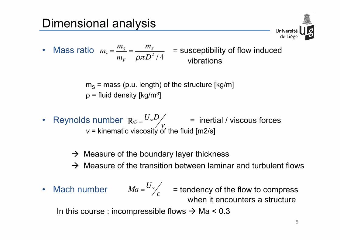
Dimensional analysis
• Mass ratio = susceptibility of flow induced vibrations mS = mass (p.u. length) of the structure [kg/m] ρ = fluid density [kg/m3]
• Reynolds number = inertial / viscous forces
ν = kinematic viscosity of the fluid [m2/s] à Measure of the boundary layer thickness à Measure of the transition between laminar and turbulent flows
• Mach number = tendency of the flow to compress
when it encounters a structure In this course : incompressible flows à Ma < 0.3 5
mr =mS
mF
=mS
ρπD2 / 4
Re =U∞Dν
Ma =U∞c

Dimensional analysis
• Damping factor (classically)
When Fluid-Structure interactions are concerned à “reduced damping” or Scruton number
6
ηS =energy dissipated per cycle
4π × total energy of the structure
m
YN YN ln YN /YN+1( ) = 2πηS
(linear system)
≈ mr ×ηS

Source FIV1977
Dimensional analysis
Motion of a linear structure in a subsonic, steady flow Described by :
7
• Geometry • Reduced velocity
• Dimensionless amplitude
• Mass ratio
• Reynolds number
• Damping factor
lD
AD
Ur
mr
Re
ηS
→ AD = F l
D,Ur, Re,mr,ηS( )
VIV Galloping (Lecture 7)

Today’s lecture
Dimensional analysis Examples of VIV Flow around static cylinders Effect of a prescribed motion of the cylinder Free vibration: VIV Modelling VIV Lock-in mechanism
8

VIV examples – in air
• Bridges
• Chimneys
• High rise buildings
9
Great-Belt bridge (Denmark)
Burj Khalifa (Dubai)
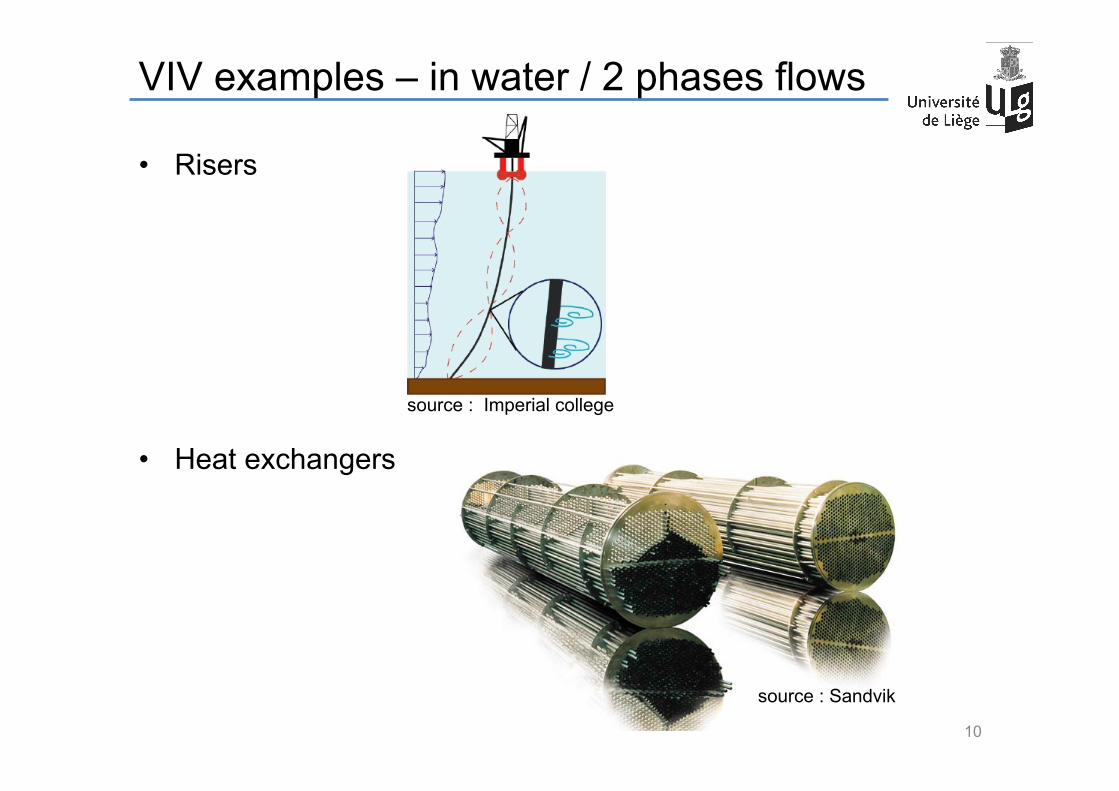
VIV examples – in water / 2 phases flows
• Risers • Heat exchangers
10
source : Imperial college
source : Sandvik

VIV examples : Great-Belt bridge
11
(Larsen 2000)
Unacceptable VIV motion (~ 40cm) during final construction stage at low (and frequent) wind speeds (~8m/s)

VIV examples : Great-Belt bridge
12
(Larsen 2000) (Frandsen 2001)
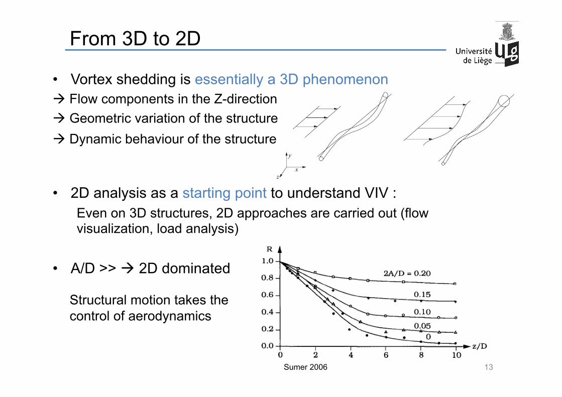
From 3D to 2D
• Vortex shedding is essentially a 3D phenomenon à Flow components in the Z-direction à Geometric variation of the structure à Dynamic behaviour of the structure • 2D analysis as a starting point to understand VIV :
Even on 3D structures, 2D approaches are carried out (flow visualization, load analysis)
• A/D >> à 2D dominated
13 Sumer 2006
Structural motion takes the control of aerodynamics

Dimensional analysis
Motion of a 2D linear structure in a subsonic, steady flow Described by : Other parameters: • Surface roughness of the structure (for rounded shapes) • Turbulence intensity of the upstream flow
à Effect on the wake, hence of the lift and on the VIV 14
→ AD = F Ur, Re,mr,ηS( )
m U∞
D
Great Belt bridge

Today’s lecture
Dimensional analysis Examples of VIV Flow around static cylinders Effect of a prescribed motion of the cylinder Free vibration: VIV Modelling VIV Lock-in mechanism
15
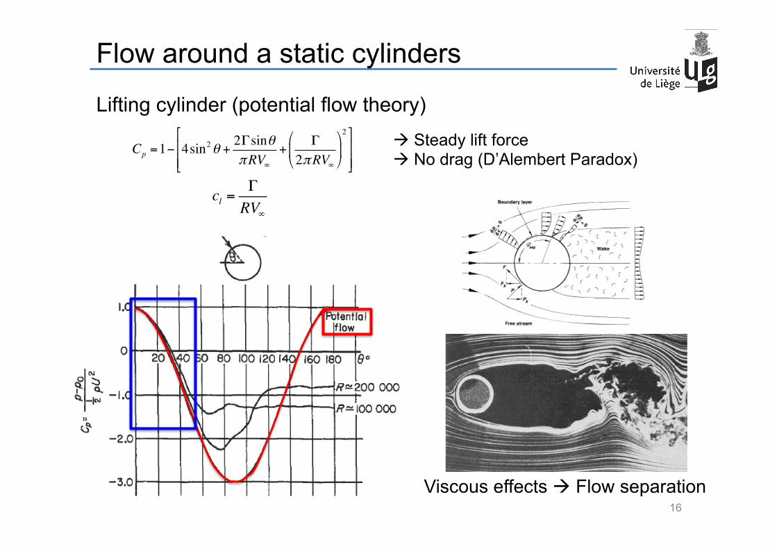
Viscous effects à Flow separation
Flow around a static cylinders
Lifting cylinder (potential flow theory)
16
Cp =1− 4sin2θ +
2ΓsinθπRV∞
+Γ
2πRV∞
$
%&
'
()
2*
+,,
-
.//
cl =ΓRV∞
à Steady lift force à No drag (D’Alembert Paradox)
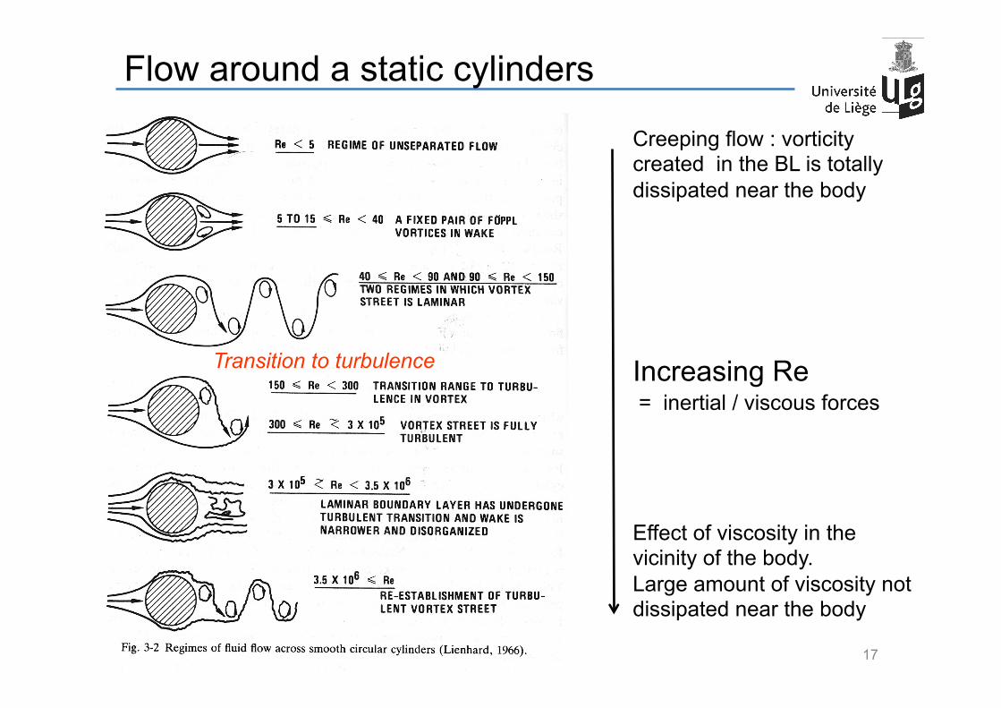
Flow around a static cylinders
17
Transition to turbulence Increasing Re = inertial / viscous forces
Creeping flow : vorticity created in the BL is totally dissipated near the body
Effect of viscosity in the vicinity of the body. Large amount of viscosity not dissipated near the body

Flow around a static cylinders How vortex shedding appears ?
18
• Flow speed outside wake is much higher than inside • Vorticity gathers in upper and lower layers • Induced velocities (due to vortices) causes this perturbation to amplify
à Origin of the vortex shedding process = shear layer instability (purely inviscid mechanism)
Vortex shedding = global instability : the whole wake is affected = robust : vorticity is continuously produced @ a well defined frequency (see Strouhal)
Flow separation

Flow around a static cylinders
19
Strouhal number fVS = shedding frequency D = cross dimension U∞ = free stream velocity à Linear dependency of the shedding frequency
with free stream velocity
à St ~ cste in a limited range of Reynolds numbers !
St ≡ fVSDU∞
0 5 10 15 20 25 300
200
400
600
U∞
f Sf VS

Aerodynamic forces à Impact of the shed vortices on the aerodynamic forces à Lift force varies at fVS
à Drag force varies at ~ 2 fVS
Sumer 2006
Flow around a static cylinders
20
L
D

Aerodynamic forces • Lift coefficient is an image of the fluctuating vorticity in the wake
(where the dominant frequency is fVS)
à CL(t) is characterized by fL and CLrms
à Dimensionless Strouhal number
• Drag coefficient : typically fD ~ 2 fVS
Flow around a static cylinders
21
CL (t) = L(t)1 / 2ρU∞
2D= 2CL
rms sin(ωLt) = 2CLrms sin(St 2πU∞
Dt)
CD (t) = D(t)1 / 2ρU∞
2D= 2CD
rms sin(ωDt) = 2CDrms sin(2ωLt) = 2CD
rms sin(2 St 2πU∞
Dt)
St = fLDU∞
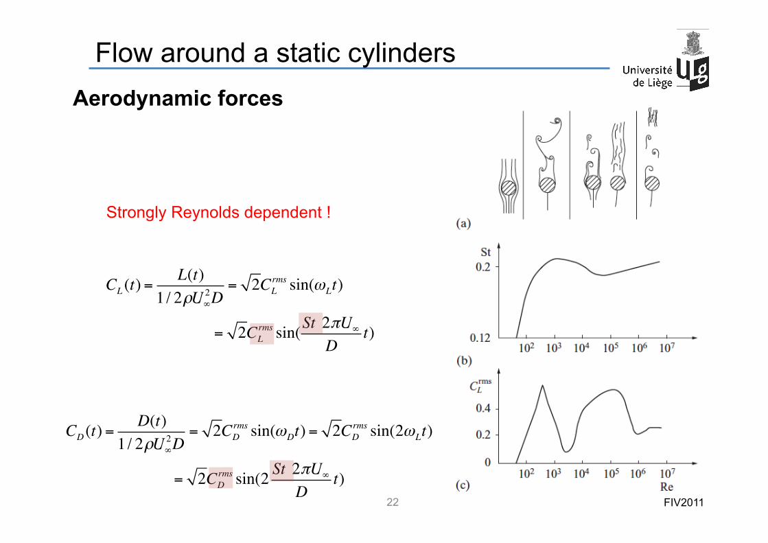
Flow around a static cylinders
22
CL (t) = L(t)1 / 2ρU∞
2D= 2CL
rms sin(ωLt)
= 2CLrms sin(St 2πU∞
Dt)
CD (t) = D(t)1 / 2ρU∞
2D= 2CD
rms sin(ωDt) = 2CDrms sin(2ωLt)
= 2CDrms sin(2 St 2πU∞
Dt)
Strongly Reynolds dependent !
Aerodynamic forces
FIV2011

Today’s lecture
Dimensional analysis Examples of VIV Flow around static cylinders Effect of a prescribed motion of the cylinder Free vibration: VIV Modelling VIV Lock-in mechanism
23

Oscillating cylinder
à Cylinder forced to move
Imposed motion :
A = Amplitude ff = Forcing frequency
Remember : Re has also a strong effect on the shedding process à Effect of the motion of the cylinder, for a given Re range.
We can observe: Change in the flow pattern and in the shedding frequency
24
y(t) = Asin(2π f f t)
Order of magnitude of the diameter (D) à A/D ~ 1
Varying around the sta?c cylinder shedding frequency (fVS0)
à 0< ff/fVS0 < 2
fVS0 = vortex shedding frequency that would be observed with cylinder at rest (i.e. following the Strouhal rela?on)

Oscillating cylinder : Patterns
• Limited range of forcing frequency and amplitude: à Two single vortices (“2S mode”)
• Higher forcing frequencies and amplitudes:
à Two pairs of vortices (“2P mode”) • Even higher frequencies and amplitudes : non-symmetric “P+S mode”
25
Williamson 2004

Oscillating cylinder : Frequency
Around ff / fVS0 ~ 1 à No change in pattern
à But effect on the shedding frequency fVS
i.e. fVS does not follow anymore the Strouhal relation
26
fVS /fVS0
ff /fVS0 1
1
fVS = ff
For a given Reynolds number and amplitude of imposed motion (A) ff is increased fVS is measured Around ff / fVS
0 ~ 1 à fVS = ff = Lock-in phenomenon
(wake capture) !! Different from lock-in in VIV !!
St = fVSDU∞
FIV2011
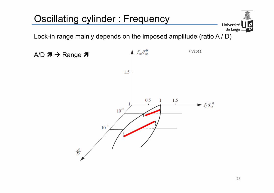
Oscillating cylinder : Frequency
Lock-in range mainly depends on the imposed amplitude (ratio A / D) A/D ì à Range ì
27

Oscillating cylinder : Lift force
Imposed motion: à The resulting lift force L(t) is not necessarily harmonic
(idem static cylinder)
But through a standard Fourier analysis, it can approximated by
= component of lift @ the forcing frequency (ff) Driving parameters: A/D and ff /fVS
0 à L0(A/D, ff /fVS0) and φ(A/D, ff /fVS
0)
Three different representations of the lift force : 1. Modulus and phase 2. Phased lift coefficients 3. Inertia and drag coefficients
28
y(t) = Asin(2π f f t)
L(t) = L0 sin(2π f f t + ϕ )

Oscillating cylinder : Lift force 1. Modulus and phase 2. Phased lift coefficients 3. Inertia and drag coefficients
29
CL (t) =CL sin(2π f f t + ϕ )
modulus phase
à both function of A/D and ff /fVS0
ff /fVS0
.5
1
CL for A/D = 0.5
2
3
4
5
0 .75 1 1.25 1.5 1.75
adapted from Carberry et al. (2005) ff /fVS
0 .5
-90
ϕ
0
90
180
270
-180 .75 1 1.25 1.5 1.75
A/D 0
max CL( )CL (A = 0)
for ff /fVS0 = 1
1
2
0 .5 1 1.5 2

Oscillating cylinder : Lift force 1. Modulus and phase 2. Phased lift coefficients 3. Inertia and drag coefficients
30
CL (t) = CL cosϕ( )sin(2π f f t)+ CL sinϕ( )cos(2π f f t)
à both function of A/D and ff /fVS0
ff /fVS0
.5
for A/D = 0.5
0
1
.75 1 1.25 1.5 1.75 adapted from Sarpkaya (1979)
ff /fVS0
.5
0
1
.75 1 1.25 1.5 1.75
in phase with (and - ) Conservative forces
y !!y in phase with Non-conservative forces à might lead to positive or
negative work
!y
CL cosϕ CL sinϕ
y(t) = Asin(2π f f t)

Oscillating cylinder : Lift force 1. Modulus and phase 2. Phased lift coefficients 3. Inertia and drag coefficients
31
CL (t) = −ρ πD2
4"
#$
%
&'CM !!y−
12ρDCD !y !y
adapted from Sarpkaya (1979)
Inertia coefficient (added mass) Link with modulus :
Drag coefficient
CM =CL cosϕUr2
2π 3 y0 D( )
As expected for Ur à 0, CM à 1 (motion in still fluid)

Today’s lecture
Dimensional analysis Examples of VIV Flow around static cylinders Effect of a prescribed motion of the cylinder Free vibration: VIV Modelling VIV Lock-in mechanism
32

Free vibration: VIV Consider a single dof system : a simple linear oscillator Remember from the dimensional analysis : In the case of free vibration, special interest for : fS = frequency of the free motion ( ‘S’ stands for Structural) fS0 = frequency of the free motion (in still fluid, i.e. U∞ = 0) A = amplitude of the free motion fVS = frequency of the vortex shedding process (with motion)
33
m U∞
D
AD = F Ur, Re,mr,ηS( )
→AD, fSfS0 ,fVSfS0
"
#$
%
&'= F Ur, Re,mr,ηS( ) Ur =
U∞
fS0D
with fS0 independent of U∞ (but not of the fluid properties)
Structural part
Fluid part

Free vibration: VIV Fixed structural parameters : D, fS0, mr, and η Fixed fluid properties : ν, ρ
34
AD, fSfS0 ,fVSfS0
!
"#
$
%&= F Ur, Re,mr,ηS( )
Airspeed effect (U∞)
For small variations of U∞ in a Re range à Neglecting the Re effect
à Ur only
FSI2011
Frequency of motion Frequency of vortex shedding

Free vibration: VIV
35
FIV1977 FSI2011
Amax Lock-‐in range
in WATER
in AIR

Free vibration: VIV Two key quantities to characterize VIV (practical interest) : • Amax : max amplitude of the y motion, reached at Ur=1/St • Lock-in range : also occurs around Ur=1/St From the dimensional analysis :
36
AD, fSfS0 ,fVSfS0
!
"#
$
%&= F Ur, Re,mr,ηS( )
→AMaxD,Lockin Ur( )
"
#$%
&'= F Re,mr,ηS( )
à Neglecting the Re effect
à mr and ηS only
à Scruton number ( ~ reduced damping) Sc = π2(1+mr )ηS
à Skop-Griffin number : SG = 4π 2St2Sc

Free vibration: VIV Amax = Function(SG) Lock-in range = Function(SG)
37
à Amax < 1 or 2 diameters (even for very low mass-damping combination)
à Amax ~ 0 for heavy/damped structures à Lock-in range ì if SG î
à VIV = Self-limited phenomenon

Today’s lecture
Dimensional analysis Examples of VIV Flow around static cylinders Effect of a prescribed motion of the cylinder Free vibration: VIV Modelling VIV Lock-in mechanism
38
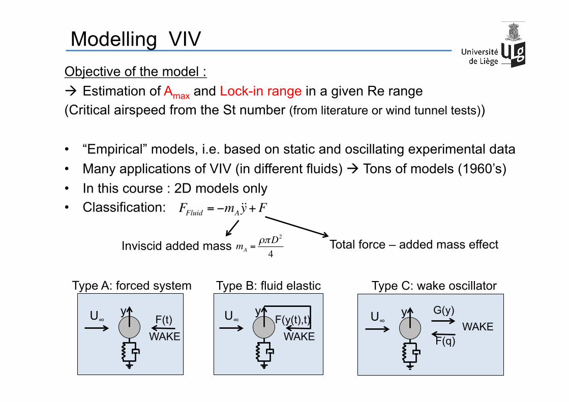
Modelling VIV Objective of the model : à Estimation of Amax and Lock-in range in a given Re range (Critical airspeed from the St number (from literature or wind tunnel tests)) • “Empirical” models, i.e. based on static and oscillating experimental data • Many applications of VIV (in different fluids) à Tons of models (1960’s) • In this course : 2D models only • Classification:
39
FFluid = −mA!!y+F
Inviscid added mass Total force – added mass effect
F(t) U∞
WAKE
y
Type A: forced system
F(y(t),t) U∞
WAKE
y
Type B: fluid elastic
F(q)
U∞ WAKE y G(y)
Type C: wake oscillator
mA =ρπD2
4
Modelling VIV Type A : Forced system models From static cylinder : = Classical linear vibration problem
40
F(t) U∞
WAKE
y
Type A
CL (t) = 2CLrms sin St 2πU∞
Dt
"
#$
%
&'
F(t) = L(t) =1/ 2ρU∞2D 2CL
rms sin St 2πU∞
Dt
"
#$
%
&'
FIV2011
à At resonance (Ur=1/St) : fVS=fS0
• Amplitude of motion inversely • proportional to damping (ζ ) • Phase jump from 0 to π • fVS follows the Strouhal relation
mS +mA( ) !!y+ 2ηS mS +mA( )ωS0 !y+ mS +mA( ) ωS
0( )2y = L(t)

Modelling VIV Type A : Forced system models OK @ large SG numbers KO @ low SG numbers No prediction of Lock-in 41
mS +mA( ) !!y+ 2ηS mS +mA( )ωS0 !y+ mS +mA( ) ωS
0( )2y = L(t) F(t) U∞
WAKE
y
Type A
y(t)D
=12π 3
CLUr2
(1+m*) 1−Ur2St2( )
2+ 4ηS
2Ur2St2( )
1/2 sin 2πStUDt +ϕ
"
#$
%
&'
AD=
CL
4π 3(1+m*)St2ηS2 =
CL
2SG
at resonance with CL=0.35
FIV2011
tanϕ = 2ηSStUr1− St2Ur2

F(y(t),t) U∞
WAKE
y
Type B
Modelling VIV Type B : Fluid elastic models à Force dependent of motion (Amplitude, displacement, velocity, acceleration, combination of them …)
Similar to galloping models (Lecture 7) à Several types exist : 1. Modified forcing model (Blevins, 1990) :
42
L(t) =1/ 2ρU∞2DCL
AD"
#$
%
&'sin St 2πU∞
Dt
"
#$
%
&'
A/D 0
max CL( )CL (A = 0) for ff /fS0 = 1
1
2
0 .5 1 1.5 2
→CLAD"
#$
%
&'=CL
0 +αAD"
#$
%
&'+β
AD"
#$
%
&'2
From oscillating cylinder (forced motion)
CL0 α and β from experiments

F(y(t),t) U∞
WAKE
y
Type B
Modelling VIV
43
L(t) =1/ 2ρU∞2DCL
AD"
#$
%
&'sin St 2πU∞
Dt
"
#$
%
&'
mS +mA( ) !!y+ 2ηS mS +mA( )ωS0 !y+ mS +mA( ) ωS
0( )2y = L(t)
CLAD!
"#
$
%&=CL
0 +αAD!
"#
$
%&+β
AD!
"#
$
%&2
AD=CL
AD!
"#
$
%&
2SG
at resonance (same than Type A)
→CL0 = α − 2SG( ) A
D#
$%
&
'(+β
AD#
$%
&
'(2
FIV2011
OK @ large SG numbers Better than Type A @ low SG numbers (underestimate !) Still no prediction of Lock-in
2nd order equation to solve for A/D à

Modelling VIV 2. Advanced forcing models:
à Amplitude and phase of the force depend on amplitude and reduced frequency of the motion à Concept of phased lift coefficients (oscillating cylinder)
Identified from imposed motion à Ur=U∞/(fD)
is valid outside coincidence
At coincidence :
44
F(y(t),t) U∞
WAKE
y
Type B
L AD,Ur, t
!
"#
$
%&=1/ 2ρU∞
2 CL cosϕAD,Ur
!
"#
$
%&sin ωt( )+CL sinϕ
AD,Ur
!
"#
$
%&cos ωt( )
(
)*
+
,-
mS!!y+ 2ηSmSωS0 !y+mS ωS
0( )2y = L A
D,Ur, t
!
"#
$
%&
AD=−CL sinϕ A /D,Ur =1/ St( )
2SG

F(y(t),t) U∞
WAKE
y
Type B
Modelling VIV 1. Modified forcing model (Blevins, 1990) :
2. Advanced forcing models :
3. Time domain fluidelastic models:
à Explicit use of the time dependence of time (Chen et al.1995)
45
L(t) =1/ 2ρU∞2DCL
AD"
#$
%
&'sin St 2πU∞
Dt
"
#$
%
&'
L AD,Ur, t
!
"#
$
%&=1/ 2ρU∞
2 CL cosϕAD,Ur
!
"#
$
%&sin ωt( )+CL sinϕ
AD,Ur
!
"#
$
%&cos ωt( )
(
)*
+
,-
L AD,Ur, y, !y, !!y
!
"#
$
%&= −m A
D,Ur
!
"#
$
%&!!y− ρU∞
2c AD,Ur
!
"#
$
%& !y− ρU∞
2k AD,Ur
!
"#
$
%&y
)
*+
,
-.+1/ 2ρU∞
2CL sin ωVSt( )
Classical fluidelastic forces (added mass, damping and stiffness) forcing term, at the frequency of vortex shedding

Modelling VIV
Problem of the Chen’s model : harmonic motion assumed, because of the
dependence of m, c and k on Ur and A/D
(identification based on oscillating cylinder experiments)
Another (much more complex) model, proposed by Simiu & Scanlan (1996)
46
L AD,Ur, y, !y, !!y
!
"#
$
%&= −m A
D,Ur
!
"#
$
%&!!y− ρU∞
2c AD,Ur
!
"#
$
%& !y− ρU∞
2k AD,Ur
!
"#
$
%&y
)
*+
,
-.+1/ 2ρU∞
2CL sin ωVSt( )
L y, !y, t( ) =1/ 2ρU∞2D c(Ur ) 1−ε
y2
D2
#
$%
&
'(!yU∞
+ k(Ur )yU∞
+CL (Ur )sin ωVSt( ))
*+
,
-.
depends on Ur only à not especially harmonic
non linear term to account for amplitude effect

Modelling VIV
47
F(t) =1/ 2ρU∞2D 2CL
rms sin St 2πU∞
Dt
"
#$
%
&'
F(t) =1/ 2ρU∞2DCL
AD"
#$
%
&'sin St 2πU∞
Dt
"
#$
%
&'
F AD,Ur, t
!
"#
$
%&=1/ 2ρU∞
2 CL cosϕAD,Ur
!
"#
$
%&sin ωt( )+CL sinϕ
AD,Ur
!
"#
$
%&cos ωt( )
(
)*
+
,-
F AD,Ur, y, !y, !!y
!
"#
$
%&= −m A
D,Ur
!
"#
$
%&!!y− ρU∞
2c AD,Ur
!
"#
$
%& !y− ρU∞
2k AD,Ur
!
"#
$
%&y
)
*+
,
-.+1/ 2ρU∞
2CL sin ωVSt( )
F y, !y, t( ) =1/ 2ρU∞2D c(Ur ) 1−ε
y2
D2
#
$%
&
'(!yU∞
+ k(Ur )yU∞
+CL (Ur )sin ωVSt( ))
*+
,
-.
F(t) U∞
WAKE
y
Type A : forced system
F(y(t),t) U∞
WAKE
y
Type B : Fluid elastic
F(q)
U∞ WAKE y G(y)
Type C : wake oscillator

Modelling VIV
Limitations of Types A and B :
1. Limited to harmonic motions (except at the price of cumbersome models (Simiu & Scanlan 1996))
à Difficult to generalize to more complex motions (multifrequencies …) à Not a major limitation, because VIV often results in quasi-harmonic
motions
2. More important: no physical interpretation of wake as a global mode
48
F(t) U∞
WAKE
y
Type A : forced system
F(y(t),t) U∞
WAKE
y
Type B : Fluid elastic
F(q)
U∞ WAKE y G(y)
Type C : wake oscillator

Modelling VIV Type C : Wake oscillator models “Fluid force is the result of the wake dynamics, itself influenced by the cylinder motion” à Coupling of two systems : CYLINDER (y variable) and WAKE (q variable) Several formulations exist for F(q), G(y), W[q(t)] and the choice for q(t) In all cases, the parameters of the models come from experiments on : • Static cylinder à Lift force à F(q)
Wake dynamics à W[q(t)] • Oscillating cylinder à Wake dynamics à G(y)
49
F(q)
U∞ WAKE y G(y)
Type C
m!!y+... = F(q)W q(t)[ ] =G(y,...)
!"#
$#
F(q) = effect of the wake on the cylinder G(y) = effect of the cylinder on the wake W[q(t)] = dynamics of the free wake
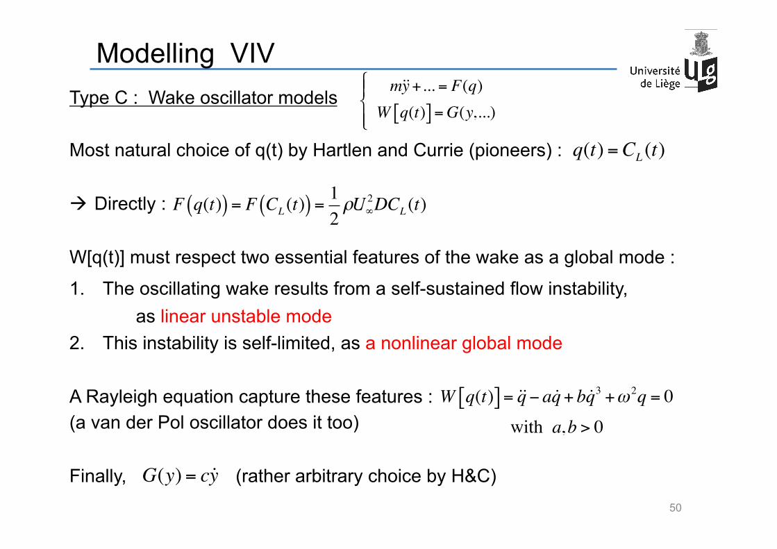
Modelling VIV Type C : Wake oscillator models Most natural choice of q(t) by Hartlen and Currie (pioneers) : à Directly :
W[q(t)] must respect two essential features of the wake as a global mode :
1. The oscillating wake results from a self-sustained flow instability, as linear unstable mode
2. This instability is self-limited, as a nonlinear global mode A Rayleigh equation capture these features : (a van der Pol oscillator does it too) Finally, (rather arbitrary choice by H&C) 50
m!!y+... = F(q)W q(t)[ ] =G(y,...)
!"#
$#
q(t) =CL (t)
F q(t)( ) = F CL (t)( ) = 12ρU∞
2DCL (t)
W q(t)[ ] = !!q− a !q+ b !q3 +ω 2q = 0with a,b > 0
G(y) = c!y

Modelling VIV Type C : Wake oscillator model by Facchinetti, de Langre & Biolley • Using the wake dof :
• Based on a van der Pol oscillator for W[q(t)]
• Using acceleration for coupling the wake to the structure
51
mS + ρD2 π
4!
"#
$
%&!!y+ cS +
12ρU∞D St CD
!
"#
$
%& !y+ kSy =
14ρU 2
∞DCL0q
!!q+ 2πStU∞
Dε q2 −1( ) !q+ 2πStU∞
D!
"#
$
%&
2
=AD!!y
)
*
++
,
++
q(t) = 2CL (t) /CL0
from force measurement in static cylinder experiments (typical values: CL0=0.3 and CD=1.2)
from wake analysis (hotwire) in static cylinder exp. (typical values : St=0.2 and ε = 0.3) from wake analysis in oscillating cylinder exp. (typical value : A = 12)

Modelling VIV Type C : Wake oscillator model by Facchinetti, de Langre & Biolley Using typical values (+CD=1) à Strong underestimation of the amplitude à But good qualitative influence of the SG parameter on the lock-in
range
52
modified forcing model
wake oscillator
forcing model
FIV2011 FIV2011
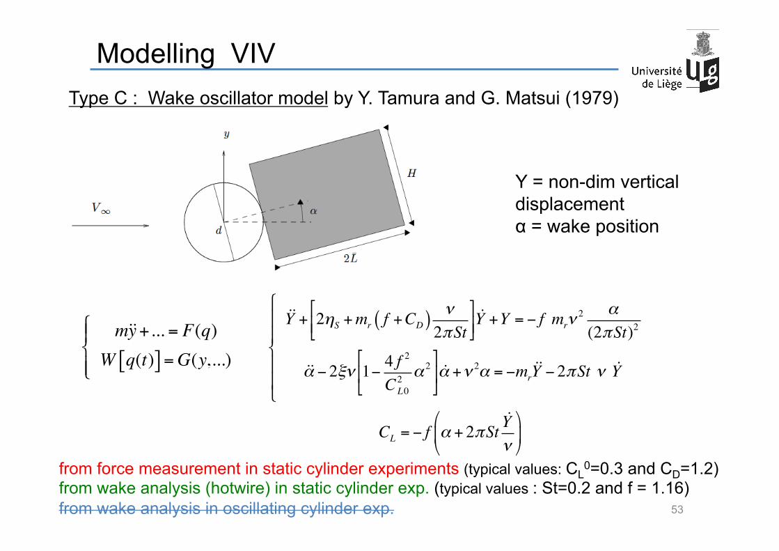
Modelling VIV Type C : Wake oscillator model by Y. Tamura and G. Matsui (1979)
53
!!Y + 2ηS +mr f +CD( ) ν2πSt
!
"#$
%&!Y +Y = − f mrν
2 α(2πSt)2
!!α − 2ξν 1− 4 f 2
C2L0
α 2!
"#
$
%& !α +ν 2α = −mr
!!Y − 2πSt ν !Y
(
)
**
+
**
m!!y+... = F(q)W q(t)[ ] =G(y,...)
!"#
$#
CL = − f α + 2πSt!Yν
"
#$
%
&'
Y = non-dim vertical displacement α = wake position
from force measurement in static cylinder experiments (typical values: CL0=0.3 and CD=1.2)
from wake analysis (hotwire) in static cylinder exp. (typical values : St=0.2 and f = 1.16) from wake analysis in oscillating cylinder exp.

Today’s lecture
Dimensional analysis Examples of VIV Flow around static cylinders Effect of a prescribed motion of the cylinder Free vibration: VIV Modelling VIV Lock-in mechanism
54

Lock-in mechanism à Link between Lock-in and linear coupled-mode flutter (L 1 & 2) (proposed by de Langre 2006) Wake oscillator model by Facchinetti, de Langre & Biolley (FLB) Non-dimensionalized : Neglecting damping and NL terms : (i.e. not responsible for lock-in)
à Ω is the only driving parameter
55
mS + ρD2 π
4!
"#
$
%&!!y+ cS +
12ρU∞D St CD
!
"#
$
%& !y+ kSy =
14ρU 2
∞DCL0q
!!q+ 2πStU∞
Dε q2 −1( ) !q+ 2πStU∞
D!
"#
$
%&
2
=AD!!y
)
*
++
,
++
!!Y +λ !Y +Y =MΩ2q
!!q+εΩ q2 −1( ) !q+Ω2q = A !!Y
#
$%
&%
t = kSmS +mF
T
Y = y /Dγ =CD / 4πSt( )Ω = St Ur
µ =mS +mF
ρD2
λ = 2ζ +γ /µ
M =CL
0
16π 2St2µ
!!Y +Y =MΩ2q!!q+Ω2q = A !!Y
"#$
%$
Ω = St Ur =fVSf
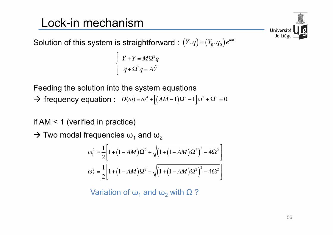
Lock-in mechanism Solution of this system is straightforward : Feeding the solution into the system equations à frequency equation :
if AM < 1 (verified in practice) à Two modal frequencies ω1 and ω2 Variation of ω1 and ω2 with Ω ?
56
!!Y +Y =MΩ2q!!q+Ω2q = A !!Y
"#$
%$
Y,q( ) = Y0,q0( )eiωt
D(ω) =ω 4 + AM −1( )Ω2 −1#$ %&ω2 +Ω2 = 0
ω12 =121+ 1− AM( )Ω2 + 1+ 1− AM( )Ω2( )
2− 4Ω2#
$%&
'(
ω22 =121+ 1− AM( )Ω2 − 1+ 1− AM( )Ω2( )
2− 4Ω2#
$%&
'(

Lock-in mechanism Depending on the sign of the radicand :
or à ω1 and ω2 are real modal frequencies à two neutrally stable modes co-exist
(neutrally because damping is neglected here)
The corresponding mode shapes :
57
ω1,22 =
121+ 1− AM( )Ω2 ± 1+ 1− AM( )Ω2( )
2− 4Ω2#
$%&
'(
1+ 1− AM( )Ω2( )2− 4Ω2 ≥ 0 Ω <
11+ AM
Y0q0=MΩ2
1−ω 2 =Ω2 −ω 2
Aω 2
Ω
de Langre 2006
11+ AM
11− AM
à close to ωR = Ω = Wake mode à close to ωR = 1 = Structural mode
Ω >1
1− AM

Lock-in mechanism
58
11+ AM
<Ω <1
1− AM
Ω
de Langre 2006
11+ AM
11− AM
ω1,2 =Ω
1+ tan2θ1± i tanθ( )
θ =12tan−1
4Ω2 − 1+ (1− AM )Ω2( )2
1+ (1− AM )Ω2
In the range Two modes exist, but with complex conjugate frequencies
à Coupled-Mode Flutter solution (CMF) = merging of two frequencies
of the neutral modes
à Range of instability one stable mode and one unstable mode

Lock-in mechanism Coupled-Mode Flutter solution (CMF) one stable mode and one unstable mode In the CMF range : - No distinction between modes - Strong deviation of the frequency of the
wake mode from ω = Ω (Strouhal relation), instead ω ~ 1
- One unstable mode instead of two well separated stable (pure wake and pure structural) modes
à CMF range ~ Lock-in range
59
11+ AM
11− AM
Ω
de Langre 2006
ωi < 0 ωi > 0
unstable
stable

Lock-in mechanism Most unstable mode ? Remember we assumed no damping : ε = λ = 0 Out of the Lock-in range, it is interesting to know which mode is dominant Considering non-zero damping : ε and λ > 0 A first order expansion of the frequency equation yields : if ω0 stands for ωW à ε and λ have a destabilization effect on the wake mode if ω0 stands for ωS à ε and λ have a damping effect on the structural mode
à in both cases the most unstable mode has the frequency of the wake mode 60
ω =ω0 + iε Ωω0
2 1−ω0
2
2(ω0
4 −Ω2 )
#
$%%
&
'((− iλ ω
0
2 Ω2 −ω0
2
2(ω0
4 −Ω2 )
#
$%%
&
'((

Lock-in mechanism à Resulting frequency of oscillation = the one of the dominant mode
i.e. the wake mode
61
AM = 0.05 AM = 0.75
Small Lock-in range Small deviation from Strouhal
Large Lock-in range Large deviation from Strouhal outside CMF
de Langre 2006

Lock-in mechanism Critical mass ratio Lock-in range = limit of CMF range : The extend of Lock-in is significantly affected by the ratio of the cylinder mass to the fluid mass : ≠ The lower Lock-in limit : The upper Lock-in limit :
62
µ =mS +mF
ρD2
11+ AM
<Ω <1
1− AM
m* =mS
ρπD2 / 4m* =
4πµ −1
ΩMIN =1
1+ AM→ St Ur
MIN = 1+ ACL0
4π 3St2 (m* +1)
#
$%%
&
'((
−1
ΩMAX =1
1− AM→ St Ur
MAX = 1− ACL0
4π 3St2 (m* +1)
$
%&&
'
())
−1
Ω
de Langre 2006

Lock-in mechanism Critical mass ratio The lower Lock-in limit : The upper Lock-in limit :
63
UrMIN =
1St
1+ ACL0
4π 3St2 (m* +1)
!
"##
$
%&&
−1
UrMAX =
1St1− ACL
0
4π 3St2 (m* +1)
"
#$$
%
&''
−1
de Langre 2006 Fixed St = 0.2 2 values for CL
0
CL0 = 0.6
CL0 = 0.3
Depend on St, m* and CL0 only
à Depending on the value of CL0, a critical value of m* exists
for which lock-in persists forever
mCRIT* =
ACL0
4π 3St2−1

Today’s lecture
Dimensional analysis Examples of VIV Flow around static cylinders Effect of a prescribed motion of the cylinder Free vibration : VIV Modelling VIV Lock-in mechanism
64

Summary • Static cylinder à strong dependence on Re • Oscillating cylinder
Strong dependence on ff/fVS0 forcing frequency
A/D forcing amplitude à Effects on the flow pattern (2S, 2P S+P modes) & vortex shedding frequency
Three different representations of the lift force : Modulus and phase Phased lift coefficients Inertia and drag coefficients
65
à lock-in
à function of A/D and ff /fVS0

Summary • Free cylinder à VIV
66
AD, fSfS0 ,fVSfS0
!
"#
$
%&= F Ur, Re,mr,ηS( )
Amax = Function(SG) Lock-in range = Function(SG) à VIV = Self-limited phenomenon
à 3 types of models: - forced system models - fluid elastic models - wake oscillator models
SG4πSt2
SG

Summary
67
F(t) U∞
WAKE
y
Type A : forced system
F(y(t),t) U∞
WAKE
y
Type B : Fluid elastic
F(q)
U∞ WAKE y G(y)
Type C : wake oscillator
F(t) =1/ 2ρU∞2D 2CL
rms sin St 2πU∞
Dt
"
#$
%
&' F A
D,Ur, y, !y, !!y
!
"#
$
%& m!!y+... = F(q)
W q(t)[ ] =G(y,...)
!"#
$#
modified forcing model
wake oscillator
forcing model
Type A B and C are empirical models Type C models the cause of the fluid forces (that types A & B take for granted)

Summary • Lock-in mechanism through linear analysis
à Coupled-Mode Flutter (CMF) • Critical mass ratio à infinite lock-in range
• Link between Airfoil flutter and Lock-in
pitch (α) and plunge (h) transverse displacement (y) and wake variable (q)
68
CL(t)
related to position of the separation point
mS + ρD2 π
4!
"#
$
%&!!y+ cS +
12ρU∞D St CD
!
"#
$
%& !y+ kSy =
14ρU 2
∞DCL0q
!!q+ 2πStU∞
Dε q2 −1( ) !q+ 2πStU∞
D!
"#
$
%&
2
=AD!!y
)
*
++
,
++
!!Y +Y =MΩ2q!!q+Ω2q = A !!Y
"#$
%$
References
• FIV1977 ‘Flow-induced vibration’, R.D. Blevins • FSI2011 ‘Fluid-structure Interactions : cross-flow induced instabilities’, M.P. Paidoussis,
S. J. Price, E. de Langre. Cambridge University Press • Williamson 2004 : C.H.K. Williamson and R. Govardhan, ‘Vortex-Induced Vibrations’,
ann. rev. Fluid Mech 2004, 36:413-55 • Larsen 2000 : A. Larsen et al. ‘Storebelt suspension bridge - vortex shedding excitation
and mitigation by guide vanes’, J. Wind Engineering and Industrial Aerodynamics 2000, 283-296
• Frandsen 2001 J.B. Frandsen, ‘Simultaneous pressures and accelerations measured full-scale on the Great Belt East suspension bridge’, , J. Wind Engineering and Industrial Aerodynamics 2001, 95-129
• Carberry et al. 2005 Carberry, J., Sheridan, J. & Rockwell, D. ‘Controlled oscillations of a cylinder: Forces and wake modes’, J.l of Fluid Mechanics 2005 538, 31–69.
• Sarpkaya 1979 Sarpkaya, T. ‘ Vortex-induced oscillations – a selective review’ J. of Applied Mechanics 1979, 46, 241–258.
• Sumer 2006 B.M. Sumer J. Fredsoe ‘Hydrodynamics around cylindrical structures’, Advanced series on ocean engineering, Vol 26, World Scientific
• de Langre 2006 E. de Langre ‘Frequency lock-in is caused by coupled-mode flutter’, J. of Fluids and structures 2006, 22, 783-791
• Y. Tamura and G. Matsui ‘Wake oscillator model of vortex induced oscillation of circular cylinder’ Proceedings of the 5th International Conference on Wind Engineering, Vol.2, Fort Collins, Colorado, USA, July 1979, pp. 1085-1092
69