Aeroelastic Preliminary Design of a 2 MW Onshore Wind Turbine with Large Capacity Factor for Low...
74
Loads, Aerodynamics and Control of Wind Turbines: 46320 Final Report: Cap50 Wind Turbine 7/12/2012 Teacher of the course: Morten Hartvig Hansen Group members: - Víctor Alcázar [email protected] - Marius Koch [email protected] - Luis Gonzales [email protected]
-
Upload
mariuskoch -
Category
Documents
-
view
126 -
download
8
description
This project contains the preliminary design of a 2 MW onshore wind turbine according to IEC-64100-1 Ed.3. The aerodynamic and structural design of the blade has been performed while the design for the remaining structural components was obtained by scaling the NREL 5 MW reference wind turbine. A reduced load set has been simulated with HAWC2 and a Campbell diagram has been created. HAWC2 is the in-house software from DTU Wind Energy for load simulations of wind turbines. The extreme and fatigue loads have been computed and the results have been assessed to work out design constrains and suggestions for a hypothetical second design iteration. The main design criterion was a high capacity factor of more than 50% for low wind speed sites (class III). A high capacity factor reduces the ratio of grid installation costs per energy production which is of big interest especially for remote areas. In order to reach a high capacity factor the nominal wind speed has to be very low in comparison to most of the commercial turbines. Thus, the rotor diameter has to be chosen relatively big for a certain level of rated power and we chose a diameter of 115 m. We separated the work and my main tasks were the specification of the global turbine parameters with the goal to archive the desired capacity factor. Furthermore, I carried out the controller implementation and the aeroelastic simulations with HAWC2. It can be mentioned that a capacity factor of 55% has been obtained for the selected wind class based on the power curve accomplished in the simulations (load case 1.1).
Transcript of Aeroelastic Preliminary Design of a 2 MW Onshore Wind Turbine with Large Capacity Factor for Low...

Loads, Aerodynamics and
Control of Wind Turbines: 46320
Final Report: Cap50 Wind Turbine
7/12/2012
Teacher of the course: Morten Hartvig Hansen
Group members:
- Víctor Alcázar [email protected]
- Marius Koch [email protected]
- Luis Gonzales [email protected]
Loads, Aerodynamics and Control of Wind Turbines: 46320
2012
----------------------------------------------------------------------------------------------------------------------------------------------- Víctor Alcazar Contreras: s111346 Marius Koch: s111396 Luís Alberto Gonzales: s111154
2
Contents
Coordinate system ............................................................................................................................................. 4
Part 1: Introduction ........................................................................................................................................... 5
Part 2: Aerodynamic design............................................................................................................................... 7
Part 2.1: 1-Point design method description. ............................................................................................... 7
Part 2.2: Airfoils selection .............................................................................................................................. 8
Part 2.3: Choice of tip speed ratio ............................................................................................................... 11
Part 2.4: Thickness decision......................................................................................................................... 12
Part 2.5: Design point selection ................................................................................................................... 13
Part 2.6: Performance of the rotor .............................................................................................................. 17
Part 2.7: Aerodynamics input files for HAWC2 ........................................................................................... 18
Part 2.8: HAWC2 test simulation ................................................................................................................. 21
Part 3: Structural turbine design ..................................................................................................................... 23
Part 3.1: Structural blade design ................................................................................................................. 23
Part 3.2: Hub design .................................................................................................................................... 34
Part 3.3: Structural nacelle/shaft/Drive-train design .................................................................................. 35
Part 3.4: Structural tower design ................................................................................................................ 39
Part 3.5 Initial check of aeroelastic model .................................................................................................. 42
Part 3.6 Tower clearance and setting of tilt and cone angle ....................................................................... 43
Part 3.7 Structural modes ............................................................................................................................ 45
Part 4: Implementation of Risø basic PI controller .......................................................................................... 46
Part 4.1: Setting of control parameters ....................................................................................................... 46
Part 4.1.1: Aerodynamic torque gains vs. pitch angle ............................................................................. 46
Part 4.1.2: Free free drive train frequency .............................................................................................. 47
Part 4.1.1: Minimum pitch angle ............................................................................................................. 48
Part 4.2: Final check of full aeroservoelastic model .................................................................................... 48
Part 5: Aero-elastic Analysis ............................................................................................................................ 53
Part 5.1: Design Load Cases ......................................................................................................................... 53
Part 5.1.1: Design load case 1.1/1.2 ........................................................................................................ 53
Part 5.1.2: Design load case 1.3 ............................................................................................................... 54

Loads, Aerodynamics and Control of Wind Turbines: 46320
2012
----------------------------------------------------------------------------------------------------------------------------------------------- Víctor Alcazar Contreras: s111346 Marius Koch: s111396 Luís Alberto Gonzales: s111154
3
Part 5.1.3: Design load case 6.1 ............................................................................................................... 54
Part 5.2: Fatigue and extreme loads under normal production. ................................................................. 54
A) Equivalent Fatigue Loads .................................................................................................................... 54
B) Accumulated 20 year fatigue loads. .................................................................................................... 58
C) Extreme load extrapolation ................................................................................................................. 59
D) Comparison with ETM maximum loads. ............................................................................................. 63
E) Compare with NordTank Results. ........................................................................................................ 64
Part 5.3: Power and thrust curves ............................................................................................................... 68
Part 5.4: Annual Energy Production ............................................................................................................ 69
Conclusions ...................................................................................................................................................... 70
Suggestions for further iterations, limitations of the current design: .................................................... 70
References: ...................................................................................................................................................... 71
Appendix: ......................................................................................................................................................... 72
A.1 Structural mesh output from becas ...................................................................................................... 72

Loads, Aerodynamics and Control of Wind Turbines: 46320
2012
----------------------------------------------------------------------------------------------------------------------------------------------- Víctor Alcazar Contreras: s111346 Marius Koch: s111396 Luís Alberto Gonzales: s111154
4
Coordinate system The coordinate systems of the aeroelastic code HAWC2 are used and presented in the figure below.
Figure 1. Coordinate systems used
There are two coordinate systems in black which are the default coordinate systems of global reference
and default wind direction. The blue coordinate systems are main body coordinate systems attached to
node 1 of the substructure, the orientation of these are fully determined by the user. The red coordinate
systems are also defined by the user, but in order to make the linkage between aerodynamic forces and
structure work these have to have the z from root to tip, x in chordwise direction and y towards the suction
side.

Loads, Aerodynamics and Control of Wind Turbines: 46320
2012
----------------------------------------------------------------------------------------------------------------------------------------------- Víctor Alcazar Contreras: s111346 Marius Koch: s111396 Luís Alberto Gonzales: s111154
5
Part 1: Introduction The main design criterion is a high capacity factor of more than 50 % for low wind speed sites onshore. A
high capacity factor reduces the ratio of grid installation costs per energy production which is of big interest
for especially remote areas and offshore installations. However, the Cap50 turbine will be designed for low
wind speed sites based on the wind distribution suggested in IEC-64100-1 Ed.3 for wind class III. A wind
turbine for low wind speed sites has commercial possibilities because there are many possible sites also in
countries with a high installed power per area as e.g. Spain or Germany. In order to reach a high capacity
factor the nominal wind speed has to be very low in comparison to most of the commercial turbines. Thus,
the rotor diameter has to be chosen relatively big for a certain rated power. An important consideration for
the design is also that the cut-out wind speed can be chosen relatively low because higher wind speeds will
not significantly increase the capacity factor on a low wind speed site.
The turbine properties have been chosen to ensure a capacity factor over 50 %. The procedure to obtain
suitable turbine properties is described in detail in the report “Wind turbine specifications for the Cap50
wind turbine: high capacity factor at low wind speed sites” which will be delivered together with this work.
The Cap50 turbine will have a nominal wind speed of 9 m/s and a cut-out wind speed of 20 m/s. It is
assumed that a low cut-out wind speed will decrease the design loads. Thus, the turbine structure can be
designed weaker, lighter and cheaper. For the Cap50 turbine the turbulence intensity is chosen to be class
C (Iref = 0.12) which is the lowest. Thus, the amount of suitable sites will decrease but for low wind speed
sites with low turbulence intensity the Cap50 will be the optimal choice. In the table below the turbine
specifications are presented.
Wind Turbine specifications
Rotor axis type HAWT Rotor position Upwind Power regulation Pitch regulated with variable speed Wind direction control Yaw actuator controlled Number of blades 3 Rated power [MW] 2 Rated wind speed [m/s] 9 Rotor diameter [m] 115 Maximum tip speed [m/s] 80 IEC Class III - C
Table 1. Wind turbine specifications summary

Loads, Aerodynamics and Control of Wind Turbines: 46320
2012
----------------------------------------------------------------------------------------------------------------------------------------------- Víctor Alcazar Contreras: s111346 Marius Koch: s111396 Luís Alberto Gonzales: s111154
6
The table below shows which team member worked on which topic.
Name Victor Alcázar
Marius Koch
Luis Gonzales
Chapter DTU code S111346 S111396 S111154
1. Introduction X X
2. Aerodynamic design
2.1 1-Point method X X X
2.2 Choice of Airfoils X
2.3 Tip speed ratio X
2.4 Thickness decision X
2.5 Cl, Cl/Cd AOA X X
2.6 Performance test X
2.7 Aerodyn. input pc/ae X
2.8 Aerodyn. hawc2 test X
3. Structural design 3.1 Blade design X
3.2 Hub design X
3.3 Shaft design X X
3.4 Tower design X
3.5 Structural hawc2 test X
3.6 Tower clearance and setting of tilt and cone angle
X
3.7 Structural modes X
4. Controller implementation
4.1 Riso Controller X
4.2 Aeroelastic hawc2 test X X X
5. Post Process 5.1 Design load cases X
5.2 Fatigue and extreme loads under normal production
X
5.3 Power and thrust curves X
5.4 Annual Energy production X
Table 2. Report work load assigned

Loads, Aerodynamics and Control of Wind Turbines: 46320
2012
----------------------------------------------------------------------------------------------------------------------------------------------- Víctor Alcazar Contreras: s111346 Marius Koch: s111396 Luís Alberto Gonzales: s111154
7
Part 2: Aerodynamic design
Part 2.1: 1-Point design method description. The rotor design method has the main task of choosing an appropriate blade chord distribution for a given
thickness and a tip speed ratio, which should have been optimized for maximum power coefficient Cp. It is
important to distinguish what is an input for this design method and what is an initial guess:
Inputs: tip speed ratio, radial distribution, thickness distribution.
Initial guesses: Angle of attack (AOA=0), tangential interference factor a’ (a’=0.001), lift coefficient
distribution (cl=0.9) lift/drag ratio (Cl/Cd=100), all constants along the blade span.
All initial guesses are to be updated through the code iterations. The inputs will remain constant. The core
iteration routine is nothing but a modified BEM code which task is to calculate the chord. It follows this
sequence of operations for each section in the blade span in a given number of optimization loops.
1 Calculate the flow angle
2 Calculate the normal and tangential force coefficients
3 Prandtl tip loss correction factor
4 Calculate optimal chord and restrict it to 4 m
5 Calculate the solidity
6 Update a and a’
7 Calculate relative thickness
8 Update the airfoil properties for the current section
9 Calculate the structural pitch angle (twist)
Table 3. Chord optimization routine.
The airfoil properties are stored in a function which contains the polynomials AOA, Cl, Cl/Cd = f(t/c) the
airfoil properties are taken from 5 NACA airfoils, its selection procedure is explained in another section. The

Loads, Aerodynamics and Control of Wind Turbines: 46320
2012
----------------------------------------------------------------------------------------------------------------------------------------------- Víctor Alcazar Contreras: s111346 Marius Koch: s111396 Luís Alberto Gonzales: s111154
8
tangential induction factor “a” is not necessary for the iteration, but is used as a check-up, it should be
optimal to 0.33 unless the chord is restricted in some point in the span.
Part 2.2: Airfoils selection The Cap50 wind turbine is a nontraditional machine, its main objective is to maintain a constant power
supply even if the wind resource does not have very high wind speeds, to reach this goal an over
dimensionalized rotor has been designed for a small power output.
This section will comment the justification of the selection of the airfoil data; based on [3] and [4], it was
followed the recommendation that for airfoils relative thickness
between 15% - 21% the NACA 63-4XX
family is suitable; similarly, for the relative thickness between 24% - 30% the FFA-W3-XXX family is
appropriate too. These airfoils are commonly used in wind turbines as stated in [6]; therefore; 5 airfoils
sections were selected, three of them with high lift characteristics and the last two are the ones in charge
of carry the structural loads of the blades; thus; they have a considerable thickness and high drag
coefficients.
Airfoil Relative thickness
NACA 63415 15 % NACA 63418 18 % NACA63421 21 % FFA-W3-241 24 % FFA-W3-301 30 %
Table 4. Airfoils choice
The criteria for the selection of the airfoils was based in two main statements, they must have a high lift-
drag ratio and they must have a linear behavior for low angles of attack (AOA) as the ones used in wind
turbine rotors. The aerodynamic characteristics (lift, drag, etc. coefficients) were obtained from the Risø
Catalogue [5], the available experimental data for the NACA634XX family airfoils was obtained with a Re #
of 3.0x10⁶, and for the FFA-W3-XXX the Re # was 1.5x10⁶.

Loads, Aerodynamics and Control of Wind Turbines: 46320
2012
----------------------------------------------------------------------------------------------------------------------------------------------- Víctor Alcazar Contreras: s111346 Marius Koch: s111396 Luís Alberto Gonzales: s111154
9
Airfoil NACA 63415 (15%)
Figure 2. Airfoil NACA 63415 aerodynamic characteristics
Airfoil NACA 63418 (18%)
Figure 3. Airfoil NACA 63418 aerodynamic characteristics

Loads, Aerodynamics and Control of Wind Turbines: 46320
2012
----------------------------------------------------------------------------------------------------------------------------------------------- Víctor Alcazar Contreras: s111346 Marius Koch: s111396 Luís Alberto Gonzales: s111154
10
Airfoil NACA 63421 (21%)
Figure 4. Airfoil NACA 63421 aerodynamic characteristics
On one hand, from Figures 2, 3 and 4, it is observed that this NACA airfoils have very good lift - drag ratios,
the three of them surpass the value of 100; surprisingly, their lift curves reach a high value almost 1.5 for all
airfoils and most important their drag coefficients are very low in the order of 0.01, this is because their low
thickness.
Airfoil FFA-W3-241 (24%)
Figure 5. Airfoil FFA-W3-241 aerodynamic characteristics

Loads, Aerodynamics and Control of Wind Turbines: 46320
2012
----------------------------------------------------------------------------------------------------------------------------------------------- Víctor Alcazar Contreras: s111346 Marius Koch: s111396 Luís Alberto Gonzales: s111154
11
Airfoil FFA-W3-301 (30%)
Figure 6. Airfoil FFA-W3-301 aerodynamic characteristics
On the other hand, the aerodynamic coefficients curves for the FFA-W3-241 and FFA-W3-301 show very
low values of lift-drag ratio (below 50) and considerably high drag coefficients; nevertheless, the main
function of these airfoils is to carry the loads of the blades and this section will be located in the inner part
of the radius rotor (small part of the blade); thus, there are suitable for our design; moreover, we want to
remark that the criteria of linearity behavior of the lift curve for low angles of attack is accomplished for all
of the five airfoils selected as can be observed from the plots above.
Part 2.3: Choice of tip speed ratio The tip speed ratio has been chosen where the maximum power coefficient is obtained.
The power coefficients for a range of tip speed ratios have been computed with a simple BEM code and the
results are depicted in the figure below. It can be observed that based on this analysis the optimal tip speed
ratio is 9.6 where the power coefficient is 44.9 %. However, in a further design iteration it might be worth
to investigate the optimal tip speed ratio again based on a flexible structure with HawcStab2 or to simulate
the power below rated wind speed with the full aeroservoelastic model for a range of tip ratios and to
compare them afterwards.

Loads, Aerodynamics and Control of Wind Turbines: 46320
2012
----------------------------------------------------------------------------------------------------------------------------------------------- Víctor Alcazar Contreras: s111346 Marius Koch: s111396 Luís Alberto Gonzales: s111154
12
Figure 7. power coefficients vs. tip speed ratio.
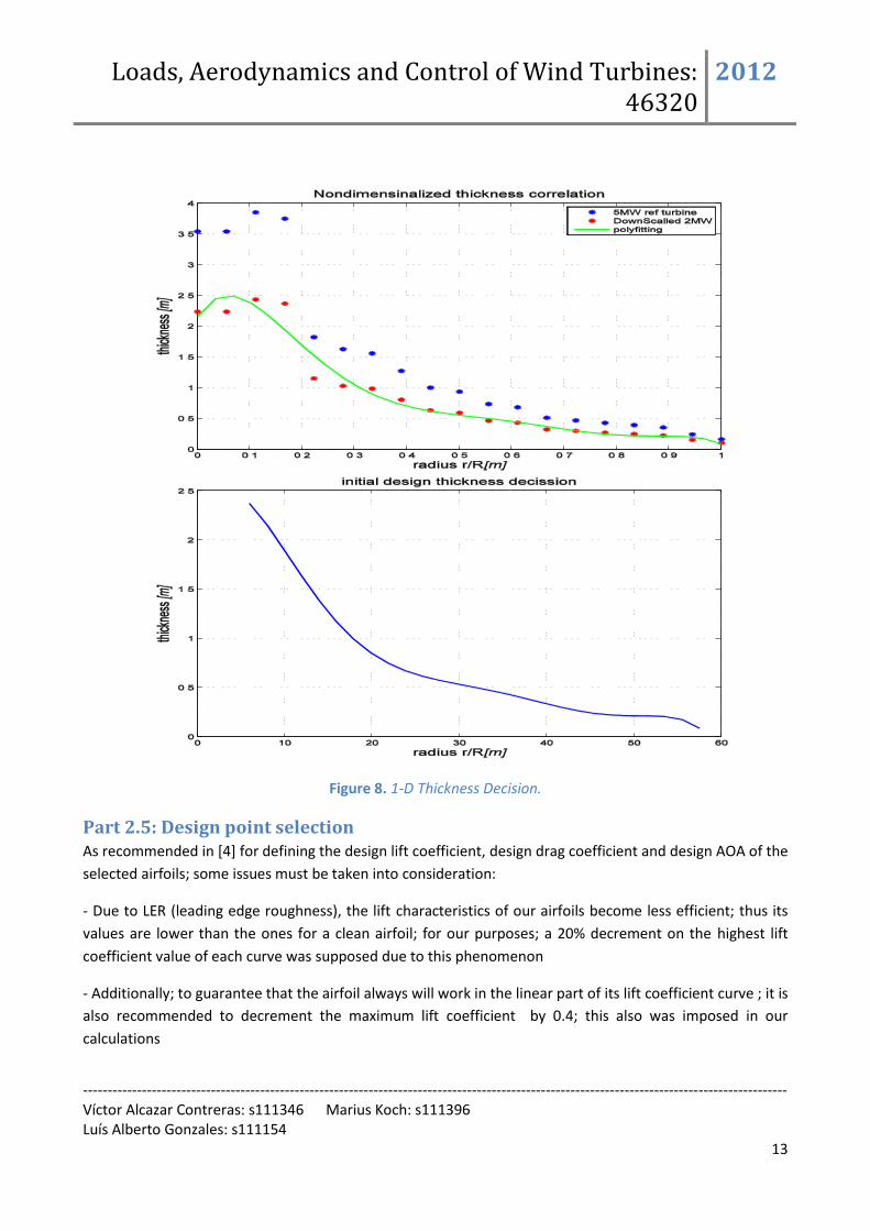
Part 2.4: Thickness decision. It was chosen in this case to start with the reference wind turbine [Nrel, 5MW] in [1]. the “_ae.txt” file
contains the chord and the relative thickness. This was the starting point. First it was calculated the
absolute thickness. From this thickness distribution, it was possible to downscale these values to the 2MW
project turbine, the scaling ratio is found in the [2].
COEF 0.632
Then a linear fitting is used to interpolate between those known values to the new radial grid chosen n=30.
Finally, a 10% root radius values are discarded (doesn´t correspond to the initial design).The process is
shown in the following figure:
Loads, Aerodynamics and Control of Wind Turbines: 46320
2012
----------------------------------------------------------------------------------------------------------------------------------------------- Víctor Alcazar Contreras: s111346 Marius Koch: s111396 Luís Alberto Gonzales: s111154
13
Figure 8. 1-D Thickness Decision.
Part 2.5: Design point selection As recommended in [4] for defining the design lift coefficient, design drag coefficient and design AOA of the
selected airfoils; some issues must be taken into consideration:
- Due to LER (leading edge roughness), the lift characteristics of our airfoils become less efficient; thus its
values are lower than the ones for a clean airfoil; for our purposes; a 20% decrement on the highest lift
coefficient value of each curve was supposed due to this phenomenon
- Additionally; to guarantee that the airfoil always will work in the linear part of its lift coefficient curve ; it is
also recommended to decrement the maximum lift coefficient by 0.4; this also was imposed in our
calculations

Loads, Aerodynamics and Control of Wind Turbines: 46320
2012
----------------------------------------------------------------------------------------------------------------------------------------------- Víctor Alcazar Contreras: s111346 Marius Koch: s111396 Luís Alberto Gonzales: s111154
14
- Finally according to [3] and[4] it was also notice that due to the LER phenomenon the drag coefficient
values also increased; thus, it was stated for our calculations that all the values of Cd increased by 40% due
to LER presence (red dotted curve).
Figure 9. Design point calculation of the airfoil NACA 63415
Figure 10. Design point calculation of the airfoil NACA 63418

Loads, Aerodynamics and Control of Wind Turbines: 46320
2012
----------------------------------------------------------------------------------------------------------------------------------------------- Víctor Alcazar Contreras: s111346 Marius Koch: s111396 Luís Alberto Gonzales: s111154
15
Figure 11. Design point calculation of the airfoil NACA 63421
Figure 12. Design point calculation of the airfoil FFA-W3-241
Figure 13. Design point calculation of the airfoil FFA-W3-301

Loads, Aerodynamics and Control of Wind Turbines: 46320
2012
----------------------------------------------------------------------------------------------------------------------------------------------- Víctor Alcazar Contreras: s111346 Marius Koch: s111396 Luís Alberto Gonzales: s111154
16
NACA 63415 NACA 63418 NACA 63421 FFA-W3-241 FFA-W3-301
t/c [%] 15 18 21 24 30 Cl_max [ ] 1.692 1.559 1.498 1.558 1.183 Cl_des [ ] 0.954 0.847 0.799 0.847 0.547 Cd_des [ ] 0.012 0.010 0.009 0.032 0.040 Cl_des/ Cd_des [ ] 80.8 85.7 89.2 26.6 13.6 AOAdes [deg] 5.4 4.8 3.9 5.2 3.5
Table 5. Design parameters for each airfoil
The values in Table 3, represent the summary results from the procedure executed for each airfoil as
described in Figures 7 to 11; from these results was possible to create the distribution of optimum AOA, lift
coefficients and lift/drag ratio along the relative thickness ratio of the airfoils assuming a maximum relative
thickness ratio of 100% in the root (cylindrical shape).
Figure 14. Relative thickness vs. Design AOA
Figure 15. Relative thickness vs. Design Cl

Loads, Aerodynamics and Control of Wind Turbines: 46320
2012
----------------------------------------------------------------------------------------------------------------------------------------------- Víctor Alcazar Contreras: s111346 Marius Koch: s111396 Luís Alberto Gonzales: s111154
17
Figure 16. Relative thickness vs. Design Cl/Cd ratio
Part 2.6: Performance of the rotor The rotor performance has been analyzed with a BEM code with the software HAWCStab2. At first the
optimal operational points without blade deflection have been computed and afterwards the steady state
power curve has been calculated, as well without blade deflection. The results for the pitch angles, rotor
speed and aerodynamic power vs. wind speed are depicted in the two figures below. The obtained pitch
angles ensure maximum aerodynamic power below and constant aerodynamic power above rated wind
speed.
Figure 17. Pitch angle (blue) and rotor speed (red) vs. wind speed computed with HAWCStab2.

Loads, Aerodynamics and Control of Wind Turbines: 46320
2012
----------------------------------------------------------------------------------------------------------------------------------------------- Víctor Alcazar Contreras: s111346 Marius Koch: s111396 Luís Alberto Gonzales: s111154
18
Figure 18. Power curve with stiff structure computed with HAWCStab2.
Part 2.7: Aerodynamics input files for HAWC2 As stated in the lectures, the rotational effect of the blade will generate an increment of the lift coefficients
of the five airfoils selected. This is produced due to when the separation of the boundary layer occurs, the
outward spanwise flow generated by the centrifugal and coriolis pumping tend to reduced the boundary
layer thickness; thus, the Cl obtained in an airfoil of a wind turbine will be higher than the one obtained in
wind tunnel static experiments; in fact, according to [9] this lift may increase by 30% due to the rotational
effects
What is more; according to [10] this effect is more significant in the inner part of the rotor (blade root)
rather than the outer part of the rotor (where the thinner airfoils are located). Therefore, it was necessary
to correct our lift coefficients curves due to the 3D stall delay effect. For this purpose the 3D correction
software ("HAWC3DProfiler081209") given by Professor C. Bak was used and here the results are showed:

Loads, Aerodynamics and Control of Wind Turbines: 46320
2012
----------------------------------------------------------------------------------------------------------------------------------------------- Víctor Alcazar Contreras: s111346 Marius Koch: s111396 Luís Alberto Gonzales: s111154
19
Figure 19. 3D Lift corrections for airfoil 63415 (AOA vs. Cl)
Figure 20. 3D Lift corrections for airfoil 63418 (AOA vs. Cl)

Loads, Aerodynamics and Control of Wind Turbines: 46320
2012
----------------------------------------------------------------------------------------------------------------------------------------------- Víctor Alcazar Contreras: s111346 Marius Koch: s111396 Luís Alberto Gonzales: s111154
20
Figure 21. 3D Lift corrections for airfoil 63421 (AOA vs. Cl)
Figure 22. 3D Lift corrections for airfoil FFA-W3-201(AOA vs. Cl)

Loads, Aerodynamics and Control of Wind Turbines: 46320
2012
----------------------------------------------------------------------------------------------------------------------------------------------- Víctor Alcazar Contreras: s111346 Marius Koch: s111396 Luís Alberto Gonzales: s111154
21
Figure 23. 3D Lift corrections for airfoil FFA-W3-301(AOA vs. Cl)
From the Figures showed above, it is observed the 2D aerodynamic data (green) and the 3D corrected
aerodynamic data (black); as it was expected according to the theory, the stall delay effect does not have a
significant effect for the thinner airfoil (located in the outer part of the rotor, 15% and 18% of relative
thickness), but for the ones close to the rotor root as the ones used in 21%, 24% and 30% a significant
increase is observed; unfortunately, the results obtained for the FFA-W3-XXX family are not entirely correct
for our point of view, it does not look realistic that the lift coefficient remains steady for so very high AOAs
as seen in Figure 18 and most drastically that even the Cl increase until 1.7 for the FFA-W3-301 airfoil. It
seems that the software provided overestimates the 3D corrections for airfoils with high chambers shape.
AOA start separation set [deg] AOA fully separation set [deg]
NACA 63415 10 25 NACA 63418 10 25 NACA 63421 7 25 FFA-W3-241 7 25 FFA-W3-301 11 30
Table 6. AOA set for 3D correction software
Part 2.8: HAWC2 test simulation In this section the input to HAWC2 is tested by simulating from cut-in to cut-out with a wind step of 2 m/s,
where the turbine is stiff, the shaft is rotating at a constant speed (bearing3), and the pitch angles are
constant. The specified rotational speeds and pitch angles are obtained with HAWCStab2 as explained in
the previous section. It shall be mentioned that the minimum pitch has been set to 0° for the HAWC2
simulations. In the figures below the power and the thrust curves are shown. It can be seen that the
aerodynamic power is lower than expected at higher wind speeds. It is assumed that the the pitch angles
are too inaccurate to ensure the expected aerodynamic power level. This could e.g. be caused by the
Loads, Aerodynamics and Control of Wind Turbines: 46320
2012
----------------------------------------------------------------------------------------------------------------------------------------------- Víctor Alcazar Contreras: s111346 Marius Koch: s111396 Luís Alberto Gonzales: s111154
22
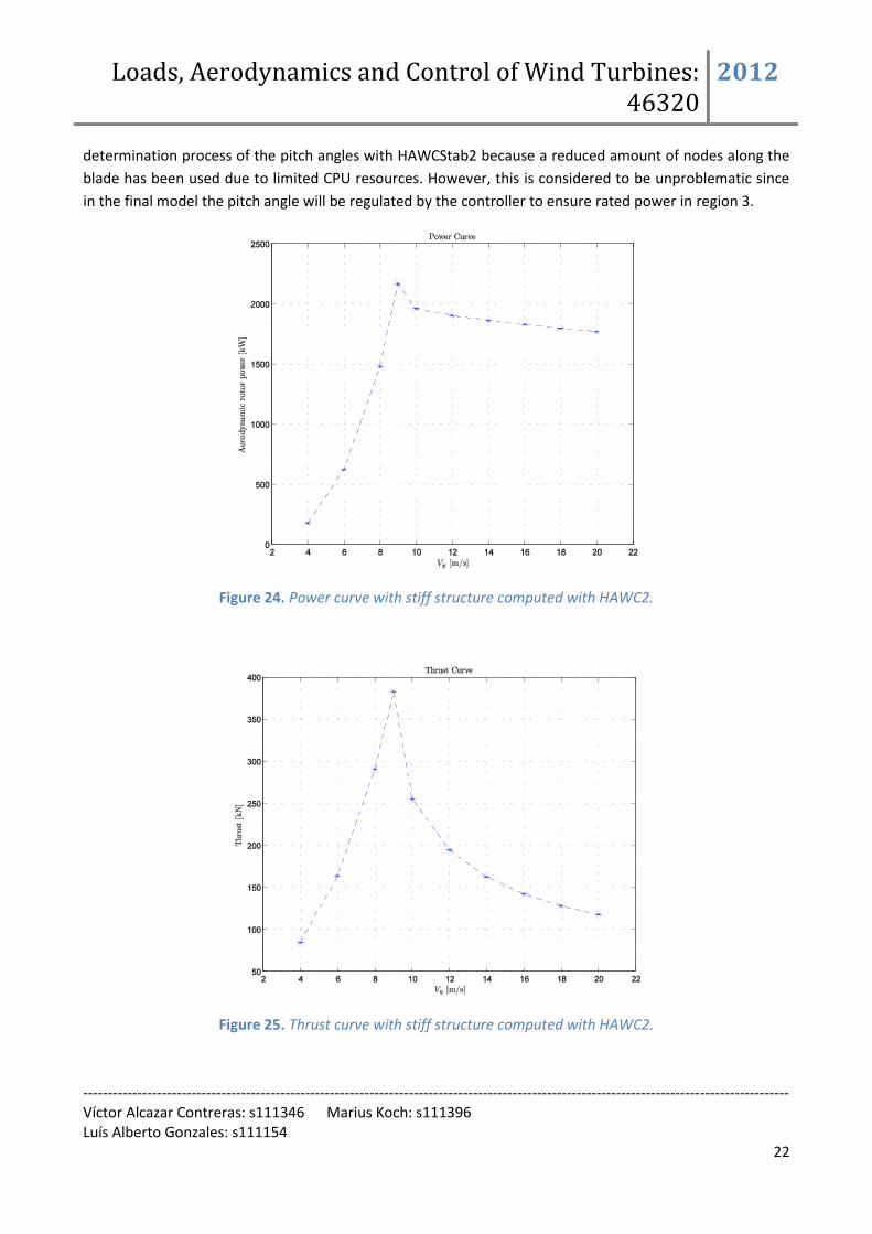
determination process of the pitch angles with HAWCStab2 because a reduced amount of nodes along the
blade has been used due to limited CPU resources. However, this is considered to be unproblematic since
in the final model the pitch angle will be regulated by the controller to ensure rated power in region 3.
Figure 24. Power curve with stiff structure computed with HAWC2.
Figure 25. Thrust curve with stiff structure computed with HAWC2.
Loads, Aerodynamics and Control of Wind Turbines: 46320
2012
----------------------------------------------------------------------------------------------------------------------------------------------- Víctor Alcazar Contreras: s111346 Marius Koch: s111396 Luís Alberto Gonzales: s111154
23
Part 3: Structural turbine design
Part 3.1: Structural blade design A) Mesh definition Process in Matlab.
Program Script: BladeRep.m main program
Support functions:
BladePlot3D.m represents 3-D arrays
progressbar.m show task queue status on window smoothFunc.m used to extend the chord distribution launch_save_airfoil.m used for generating circular airfoil, and prepare .mat files to
import the airfoils into matlab.
Table 7. Main Airfoil Coordinate Generation scripts
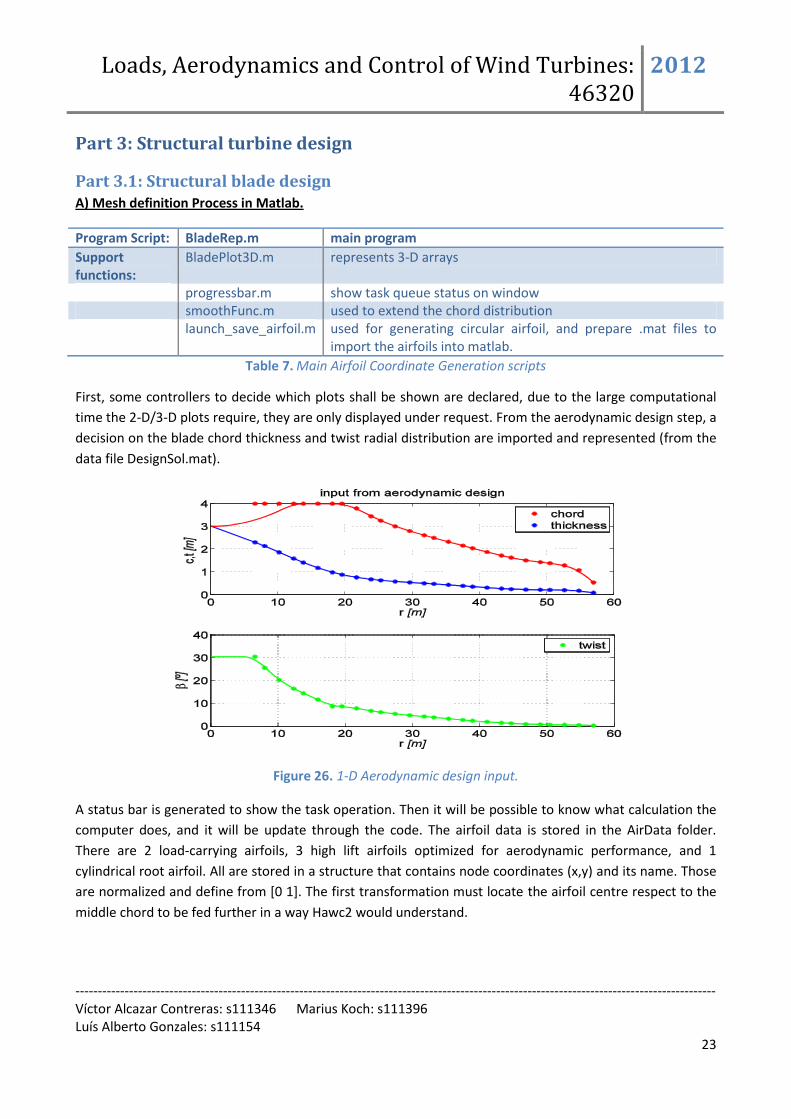
First, some controllers to decide which plots shall be shown are declared, due to the large computational
time the 2-D/3-D plots require, they are only displayed under request. From the aerodynamic design step, a
decision on the blade chord thickness and twist radial distribution are imported and represented (from the
data file DesignSol.mat).
Figure 26. 1-D Aerodynamic design input.
A status bar is generated to show the task operation. Then it will be possible to know what calculation the
computer does, and it will be update through the code. The airfoil data is stored in the AirData folder.
There are 2 load-carrying airfoils, 3 high lift airfoils optimized for aerodynamic performance, and 1
cylindrical root airfoil. All are stored in a structure that contains node coordinates (x,y) and its name. Those
are normalized and define from [0 1]. The first transformation must locate the airfoil centre respect to the
middle chord to be fed further in a way Hawc2 would understand.
Loads, Aerodynamics and Control of Wind Turbines: 46320
2012
----------------------------------------------------------------------------------------------------------------------------------------------- Víctor Alcazar Contreras: s111346 Marius Koch: s111396 Luís Alberto Gonzales: s111154
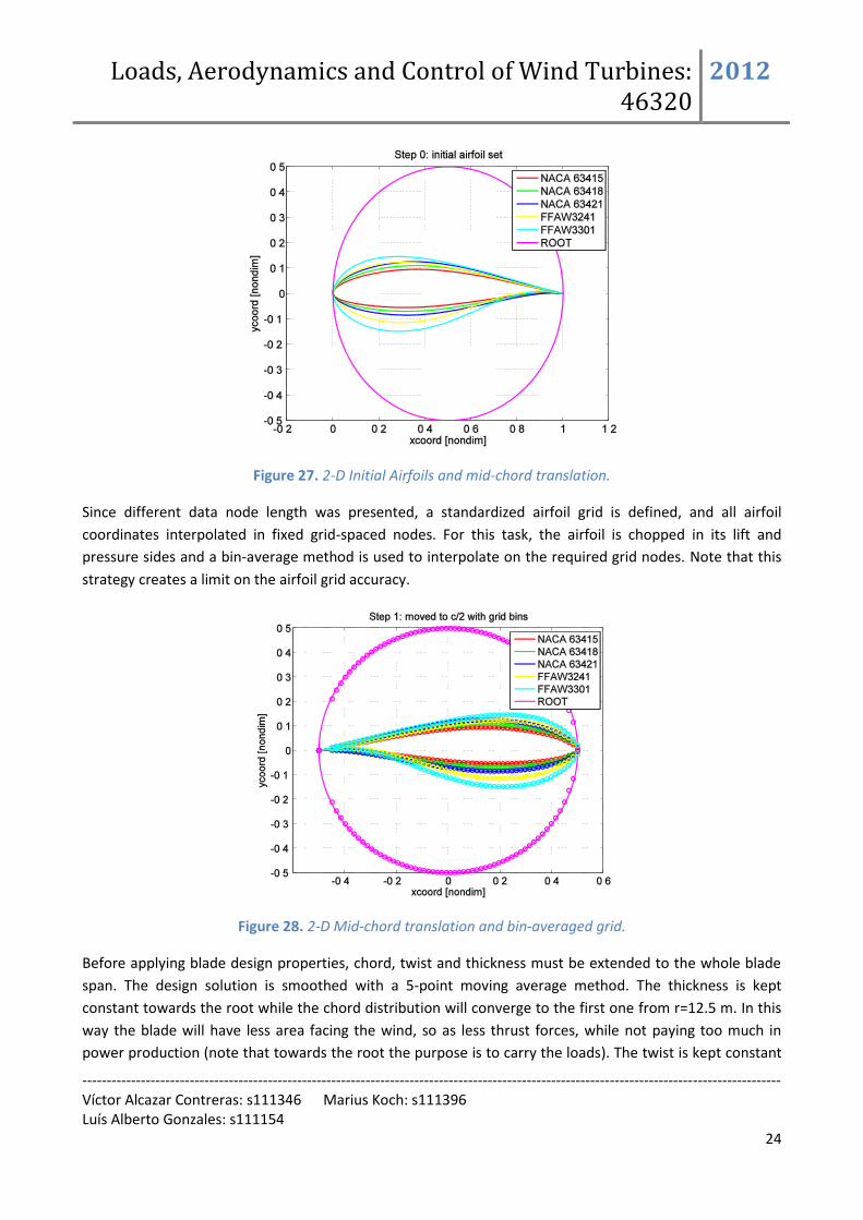
24
Figure 27. 2-D Initial Airfoils and mid-chord translation.
Since different data node length was presented, a standardized airfoil grid is defined, and all airfoil
coordinates interpolated in fixed grid-spaced nodes. For this task, the airfoil is chopped in its lift and
pressure sides and a bin-average method is used to interpolate on the required grid nodes. Note that this
strategy creates a limit on the airfoil grid accuracy.
Figure 28. 2-D Mid-chord translation and bin-averaged grid.
Before applying blade design properties, chord, twist and thickness must be extended to the whole blade
span. The design solution is smoothed with a 5-point moving average method. The thickness is kept
constant towards the root while the chord distribution will converge to the first one from r=12.5 m. In this
way the blade will have less area facing the wind, so as less thrust forces, while not paying too much in
power production (note that towards the root the purpose is to carry the loads). The twist is kept constant

Loads, Aerodynamics and Control of Wind Turbines: 46320
2012
----------------------------------------------------------------------------------------------------------------------------------------------- Víctor Alcazar Contreras: s111346 Marius Koch: s111396 Luís Alberto Gonzales: s111154
25
as well. Check figure [26] about aerodynamic design solution. Now the airfoils are to be located in the blade
span. Therefore, their relative thickness is calculated, and compared to the blade relative t/c distribution. In
a plot is shown the place of the input airfoils along the blade.
Figure 29. 1-D Input airfoils place in the blade.
The rest will be interpolation of the former ones. Indeed, the interpolated airfoil coordinates are found
through the relative thickness interpolated ratio between the two initial airfoils closer in t/c in the span.
Once the interpolation is done it is simple to scale the airfoils with the chord distribution, c(r) just by
multiplying (x,y) nodal coordinates by this magnitude. The airfoil coordinates now are ready to be exported
to BECAS.
Figure 30. 2-D Airfoil Interpolation and c(r) scaling.
Loads, Aerodynamics and Control of Wind Turbines: 46320
2012
----------------------------------------------------------------------------------------------------------------------------------------------- Víctor Alcazar Contreras: s111346 Marius Koch: s111396 Luís Alberto Gonzales: s111154
26
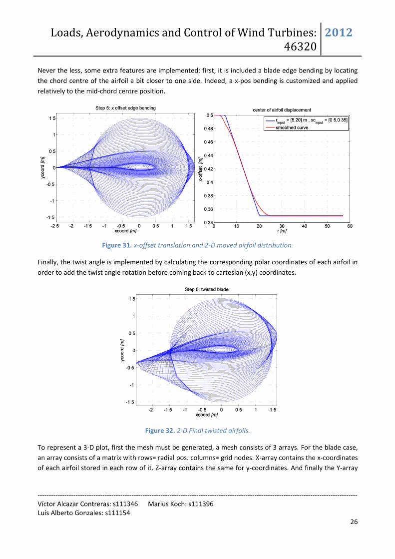
Never the less, some extra features are implemented: first, it is included a blade edge bending by locating
the chord centre of the airfoil a bit closer to one side. Indeed, a x-pos bending is customized and applied
relatively to the mid-chord centre position.
Figure 31. x-offset translation and 2-D moved airfoil distribution.
Finally, the twist angle is implemented by calculating the corresponding polar coordinates of each airfoil in
order to add the twist angle rotation before coming back to cartesian (x,y) coordinates.
Figure 32. 2-D Final twisted airfoils.
To represent a 3-D plot, first the mesh must be generated, a mesh consists of 3 arrays. For the blade case,
an array consists of a matrix with rows= radial pos. columns= grid nodes. X-array contains the x-coordinates
of each airfoil stored in each row of it. Z-array contains the same for y-coordinates. And finally the Y-array

Loads, Aerodynamics and Control of Wind Turbines: 46320
2012
----------------------------------------------------------------------------------------------------------------------------------------------- Víctor Alcazar Contreras: s111346 Marius Koch: s111396 Luís Alberto Gonzales: s111154
27
(length) is simply how far in the span the airfoils lay (repeated value of the airfoil radial position per row).
Then surf is used to represent the arrays.
Figure 33. 3-D Final twisted blade.
B) Export to BECAS and keypoint definition.
Program Script: BladeRep.m main program
Support functions: bladeKPWireframe3D.m generate a wireframe 3-D model with keypoints OutputDataFileWriter.m
creates input for python script
BECASinputGenerator.m
automatic system call to python script for each airfoil
runBECASloop.m
runs BECAS and its output function to hawc2
Table 8. BECAS communication scripts.
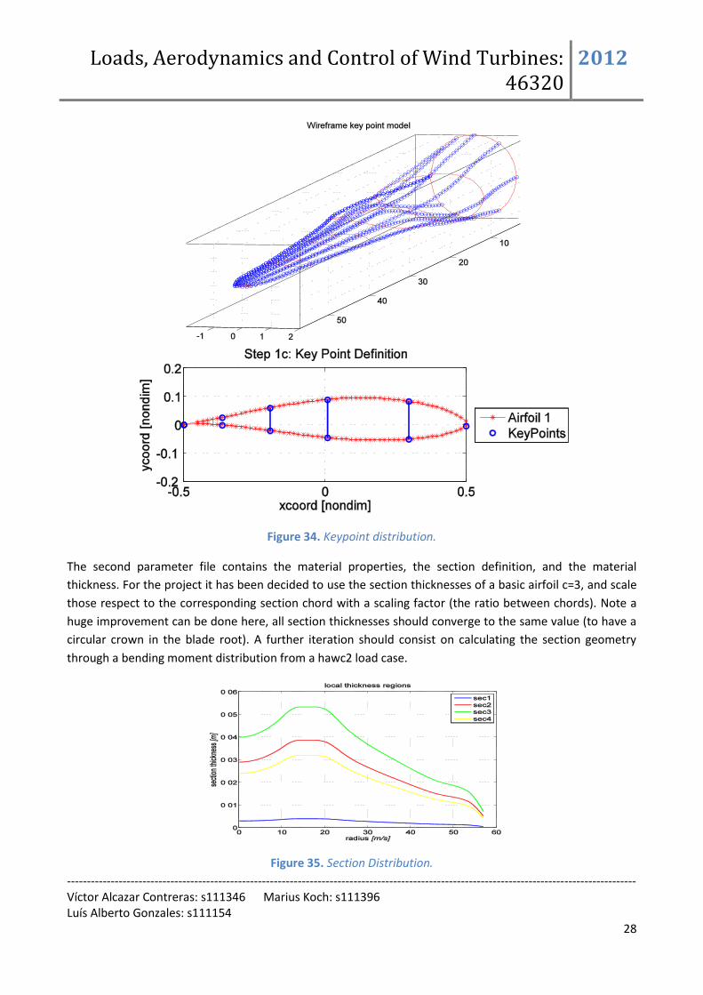
In the following figures the airfoil keypoints are defined. The wireframe is made of the keypoint lines along
the airfoils. The blade design project has 3 shear webs. However, the material does not change in the
section where the first shear web is placed, no keypoint is defined for such shear web joint. An export
feature to BECAS “OutputDataFileWriter.m” is a script able to take all the scaled airfoils respect to the
chord with the keypoint definition and the section definition, to write two text files containing inputs for
BECAS per section. The first one contains the coordinates and the KP definition.
Loads, Aerodynamics and Control of Wind Turbines: 46320
2012
----------------------------------------------------------------------------------------------------------------------------------------------- Víctor Alcazar Contreras: s111346 Marius Koch: s111396 Luís Alberto Gonzales: s111154
28
Figure 34. Keypoint distribution.
The second parameter file contains the material properties, the section definition, and the material
thickness. For the project it has been decided to use the section thicknesses of a basic airfoil c=3, and scale
those respect to the corresponding section chord with a scaling factor (the ratio between chords). Note a
huge improvement can be done here, all section thicknesses should converge to the same value (to have a
circular crown in the blade root). A further iteration should consist on calculating the section geometry
through a bending moment distribution from a hawc2 load case.
Figure 35. Section Distribution.
Loads, Aerodynamics and Control of Wind Turbines: 46320
2012
----------------------------------------------------------------------------------------------------------------------------------------------- Víctor Alcazar Contreras: s111346 Marius Koch: s111396 Luís Alberto Gonzales: s111154
29
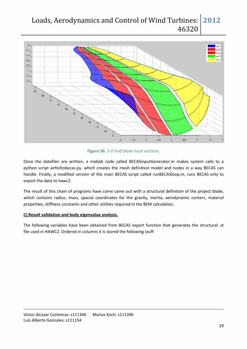
Figure 36. 3-D half blade local sections.
Once the datafiles are written, a matlab code called BECASinputGenerator.m makes system calls to a
python script airfoiltobecas.py, which creates the mesh definition model and nodes in a way BECAS can
handle. Finally, a modified version of the main BECAS script called runBECASloop.m, runs BECAS only to
export the data to hawc2.
The result of this chain of programs have come came out with a structural definition of the project blade,
which contains radius, mass, spacial coordinates for the gravity, inertia, aerodynamic centers, material
properties, stiffness constants and other utilities required in the BEM calculation.
C) Result validation and body eigenvalue analysis.
The following variables have been obtained from BECAS export function that generates the structural .st
file used in HAWC2. Ordered in columns it is stored the following stuff:
Loads, Aerodynamics and Control of Wind Turbines: 46320
2012
----------------------------------------------------------------------------------------------------------------------------------------------- Víctor Alcazar Contreras: s111346 Marius Koch: s111396 Luís Alberto Gonzales: s111154
30
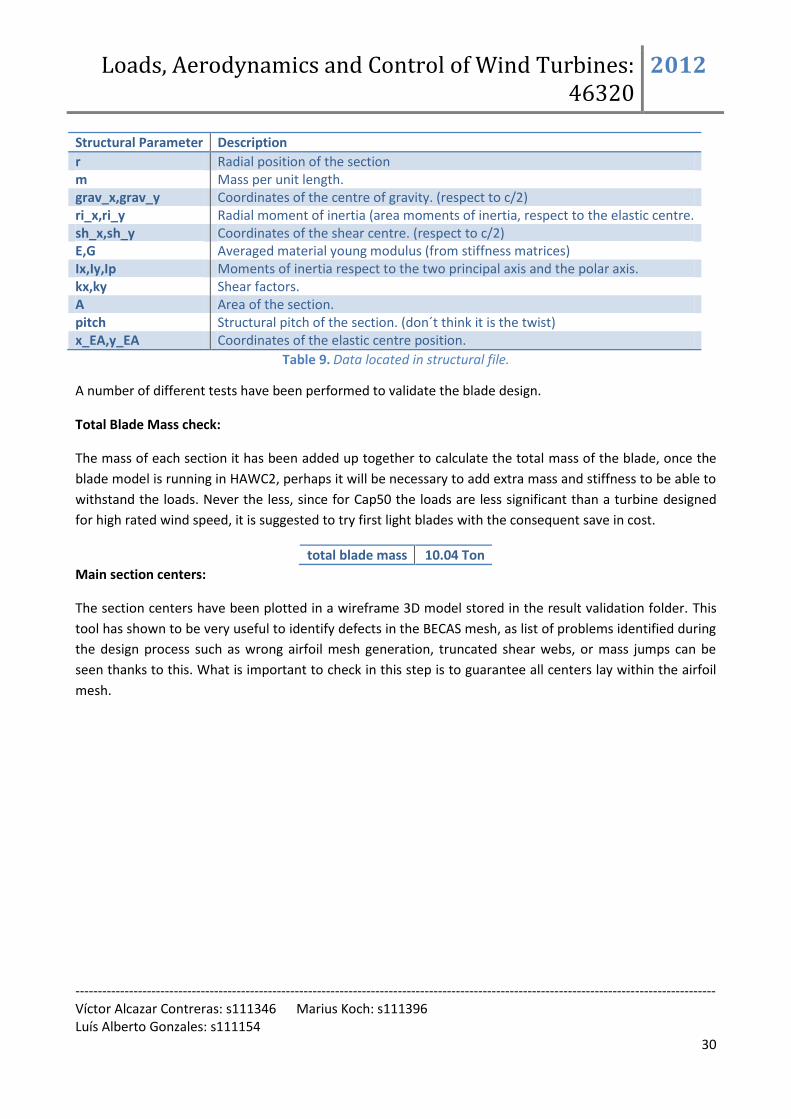
Structural Parameter Description
r Radial position of the section m Mass per unit length. grav_x,grav_y Coordinates of the centre of gravity. (respect to c/2) ri_x,ri_y Radial moment of inertia (area moments of inertia, respect to the elastic centre. sh_x,sh_y Coordinates of the shear centre. (respect to c/2) E,G Averaged material young modulus (from stiffness matrices) Ix,Iy,Ip Moments of inertia respect to the two principal axis and the polar axis. kx,ky Shear factors. A Area of the section. pitch Structural pitch of the section. (don´t think it is the twist) x_EA,y_EA Coordinates of the elastic centre position.
Table 9. Data located in structural file.
A number of different tests have been performed to validate the blade design.
Total Blade Mass check:
The mass of each section it has been added up together to calculate the total mass of the blade, once the
blade model is running in HAWC2, perhaps it will be necessary to add extra mass and stiffness to be able to
withstand the loads. Never the less, since for Cap50 the loads are less significant than a turbine designed
for high rated wind speed, it is suggested to try first light blades with the consequent save in cost.
total blade mass 10.04 Ton
Main section centers:
The section centers have been plotted in a wireframe 3D model stored in the result validation folder. This
tool has shown to be very useful to identify defects in the BECAS mesh, as list of problems identified during
the design process such as wrong airfoil mesh generation, truncated shear webs, or mass jumps can be
seen thanks to this. What is important to check in this step is to guarantee all centers lay within the airfoil
mesh.

Loads, Aerodynamics and Control of Wind Turbines: 46320
2012
----------------------------------------------------------------------------------------------------------------------------------------------- Víctor Alcazar Contreras: s111346 Marius Koch: s111396 Luís Alberto Gonzales: s111154
31
Figure 37. Main Blade center coordinates.
Middle Chord line:
One of the HTC input file for the blade consists on the mid-chord position centre. In a first iteration this
value is calculated from pure geometry calculation using the airfoil section node coordinates. Once the
model in hawc2 is running, the blade y-deflection is calculated for 5 m/s and used as feedback to decide a
blade flap pre-bending. The figure below shows the mid-chord centre coordinates before and after this
step.
Figure 38. Mid-chord (x,y) coordinates and pre-bending.

Loads, Aerodynamics and Control of Wind Turbines: 46320
2012
----------------------------------------------------------------------------------------------------------------------------------------------- Víctor Alcazar Contreras: s111346 Marius Koch: s111396 Luís Alberto Gonzales: s111154
32
Export to HTC file
The blade node definition in the input file for hawc2 should contain nodes where the most important
changes in the blade properties are found, but not so many not to make the simulations too slow. For this
blade 30 sections will be sufficient. The mass per length distribution has been used to measure the input to
hawc2, and in its figure it can be checked all significant change in the mass is described with a node. It has
been developed an automatic “htc” file generator in Matlab, able to write output text HTC files which
contains the whole blade module.
Figure 39. HTC node definition through mass per length distribution.
Modal Analysis of the blade
The last adjustment done on the blade before being able to run in the model is to tune the damping
coefficients. First all of those were settled to zero, and the last 3 can be located to obtain proper
logarithmic decrements using the structure “eigenanalysis” of hawc2. Another eigenvalue problem has
been performed in hawcstab2. Both algorithms must come out with the same natural frequencies and
logarithmic decrements, if the model is settled properly. (This means the logarithmic decrements fed into
the Hawcstab2 frame must be the same as the ones obtained in the “eigenanalysis”).
Logarithmic decrements distribution 1.1 1.40 2.7 3.8 5.5 8.6 9.6
Damping Coeff distribution chosen 0 0 0 8e-4 8e-4 8e-4
Table 10. List of logarithmic decrements obtained for the first mode.

Loads, Aerodynamics and Control of Wind Turbines: 46320
2012
----------------------------------------------------------------------------------------------------------------------------------------------- Víctor Alcazar Contreras: s111346 Marius Koch: s111396 Luís Alberto Gonzales: s111154
33
Characterization of the modes shown in hawcstab2:
Mode nr. Natural frequency Log. Decrement Type Identified
1 6.64558E-01 1.04943E+00 First Flap 2 8.03275E-01 1.26848E+00 First Edge 3 1.62643E+00 2.56836E+00 Second Flap 4 2.22861E+00 3.51929E+00 Second Edge 5 3.27514E+00 5.17189E+00 Flap 6 5.11565E+00 8.07831E+00 Torsion
Table 11. Modal analysis blade output results.
It is important to link the modal response of the blade with its structural properties. The frequencies are
affected mainly by the stiffness cross-sectional properties, and the section mass. Moreover, the blade´s
inertia plays the main role in how stiff the blade is. To avoid structural resonances with multiples of P, or
the other component modes, the blade frequencies must be placed wisely within the frequency spectrum,
not to overlap with others. The logarithmic decrement represent how fast the vibration decays, it is tuned
in hawc2 with the structural damping coefficients. Note the logarithmic decrement is independent from the
frequency.
Further development steps.
1. Use of an ultimate load case with its corresponding load distribution to recover the local blade surface
stresses, so as to check the ultimate stress limit is not overload.
2. Control the cap section thickness and width in order to manipulate the blade stiffness and mass
properties, not to allow large blade deflections in higher wind speeds.
3. Buckling analysis, adjust width of the shear webs to reduce trailing edge section width (since it contribute
less to the blade stiffness)
4. Adjust the blade section thicknesses towards the root for a more realistic joint (the bolts currently
cannot be screwed).
In the appendix documentation about the BECAS airfoil mesh is placed for some sections.

Loads, Aerodynamics and Control of Wind Turbines: 46320
2012
----------------------------------------------------------------------------------------------------------------------------------------------- Víctor Alcazar Contreras: s111346 Marius Koch: s111396 Luís Alberto Gonzales: s111154
34
Part 3.2: Hub design For the hub design, it was decided to applied a tri-cylindrical approach; the radial dimension of the hub was
taken from the downscaling excel sheet using a scale factor (SF) of 0.913, corresponding to a 115 m rotor
diameter or 4.17 MW wind turbine.
From this excel sheet the following useful information was taken:
Hub characteristics
Hub Diameter [m] 2.74 Total hub mass [kg] 43168.1 Total hub inertia about yaw axis [kgm2] 73416.5
Table 12. Hub characteristics
Figure 40. Hub dimensions.
From the Table and Figure showed above, it can be deduced that the inputs for HAWC2 will consist in three
cylinders (modeled as 3 beams of 1.37m of length) attached in one of its extreme nodes (center of the
hub); forming together the tri-cylindrical hub. Therefore in ".st file" for HAWC2 input, a distributed mass
and area moments of inertia were used along the length of each cylindrical part of the hub. Furthermore,
an outer diameter of 3m of each cylinder was selected due to this corresponds to the root diameter of the
blade, and a thickness of 0.20m was assumed for each cylinder too (flange part). Moreover, the distance of
each cylinder was divided in 3 subsections (4 nodes) of equal length (0.457 m)
Taking a density of 5970 kg/m3 [11] for the ductile iron material used in the manufacture of this type of
components, the following parameters were inputted as the flexible case for the hub:

Loads, Aerodynamics and Control of Wind Turbines: 46320
2012
----------------------------------------------------------------------------------------------------------------------------------------------- Víctor Alcazar Contreras: s111346 Marius Koch: s111396 Luís Alberto Gonzales: s111154
35
Structural Parameter Calculation procedure
Density [kg/m3] 5970 Linear mass [kg/m] 1.05x10⁴ grav_x,grav_y (0,0) centered cylindrical crown ri_x,ri_y [m]
(
,
) = ( )
sh_x,sh_y (0,0) centered cylindrical crown E,G [Pa, Pa] ( , ) ductile iron Young and Shear modulus Ix,Iy,Ip [m4] (
,
) = (1.73,1.73,3.47)
kx,ky (0.5,0.5) A [m2]
= 1.76
pitch 0 (No structural pitch) x_EA,y_EA (0,0) centered cylindrical crown
Table 13. Hub structural parameters for .st file
Additionally as recommended in class, the same damping coefficients calculated for the blade were
assumed for the hub in the .htc file for HAWC2 input. Due to in our procedure the mass and the inertias are
distributed on each cylinder, there was not necessity to applied concentrated mass or inertias in the .htc
code for the HAWC simulations for the hub specifically.
Mx My Mz Kx Ky Kz
Damping Coeff. distribution chosen 0 0 0 8x10⁻⁴ 8x10⁻⁴ 8x10⁻⁴
Table 14. Hub damping coefficients for .htc file
Part 3.3: Structural nacelle/shaft/Drive-train design A) Nacelle Basic design decision.
The "tower top" hawc2 body element is nothing but the nacelle structure. Due to the complex of this
system and the limited time available, it is assumed a cylindrical metal piece which will have similar
structural properties than the real structure, but with artificial concentrated mass and inertia. Obviously, a
more detailed model of the nacelle could provide a deep understanding of the system components
interaction.
The tower top length is chosen from the scaling spreadsheet with the reference model Nrel 5MW wind
turbine using again the SF = 0.913. It represents the distance from the last element of the tower, and the
first element of the shaft. The tower top diameter comes from the outer diameter of the last node from the
tower design, this would make easy to attach the tower node distribution to its top, but it is just a
convention. The tower top thickness is chosen to be an average value between the tower bottom and top
thicknesses.

Loads, Aerodynamics and Control of Wind Turbines: 46320
2012
----------------------------------------------------------------------------------------------------------------------------------------------- Víctor Alcazar Contreras: s111346 Marius Koch: s111396 Luís Alberto Gonzales: s111154
36
parameter value
length 1.79 m outer diameter 3.00 m top thickness 0.02 m
Table 15. Tower top basic geometry
Note this component only has 0.001 kg/m mass per section length since it is only intended to connect
tower and shaft node distributions. However, to make the model realistic, a concentrated mass must be
included externally, so the weight of the nacelle will count on the simulation. The command in the hawc2
input file is “concentrated_mass”.
concentrated mass concentrated inertia
on node 2 2 offset coordinates (zt,xt,yt) m respect to node
(0.0 1.73 0.19) nacelle c.o.m. (0.0 0.0 0.0) tower axis.
value 182464.65 1651588.20
Table 16. Concentrated nacelle mass and inertia
The nacelle centre of mass space location come from the scaling spreadsheet (where the concentrated
mass must be placed), as well as the nacelle weight and its inertia. Note the inertia is placed on the last
tower-top node. This is because in the scaling spreadsheet the Steiner´s theorem is used to transfer the
inertia moment respect to the nacelle centre of mass, to the tower top axis.
The nacelle mass estimation was based on the downscaling excel sheet assuming a wind turbine output
power of 4.17 MW (equivalent to a rotor diameter of 115 m); even though, the power output is not the
stated for the Cap50 wind turbine (2MW); the nacelle structure should be able to withstand the weight and
aerodynamic loads of the components like rotor, shaft, main bearing, etc. designed for a rotor of huge
dimensions. Therefore the downscaling factor for this analysis was 0.913 and the nacelle mass was
182464.7 kg
Loads, Aerodynamics and Control of Wind Turbines: 46320
2012
----------------------------------------------------------------------------------------------------------------------------------------------- Víctor Alcazar Contreras: s111346 Marius Koch: s111396 Luís Alberto Gonzales: s111154
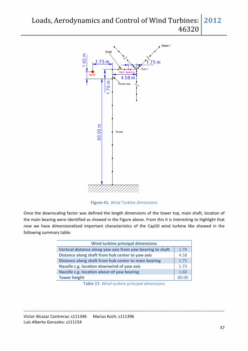
37
Figure 41. Wind Turbine dimensions
Once the downscaling factor was defined the length dimensions of the tower top, main shaft, location of
the main bearing were identified as showed in the Figure above. From this it is interesting to highlight that
now we have dimensionalized important characteristics of the Cap50 wind turbine like showed in the
following summary table:
Wind turbine principal dimensions
Vertical distance along yaw axis from yaw bearing to shaft 1.79 Distance along shaft from hub center to yaw axis 4.58 Distance along shaft from hub center to main bearing 1.75 Nacelle c.g. location downwind of yaw axis 1.73 Nacelle c.g. location above of yaw bearing 1.60 Tower height 80.00
Table 17. Wind turbine principal dimensions

Loads, Aerodynamics and Control of Wind Turbines: 46320
2012
----------------------------------------------------------------------------------------------------------------------------------------------- Víctor Alcazar Contreras: s111346 Marius Koch: s111396 Luís Alberto Gonzales: s111154
38
Shaft/Drivetrain design decision
For the design of the main shaft, one more time, the downscaling excel sheet was taken in consideration,
with some slight modification in the procedure, a special procedure was applied. First of all, for the case of
the drivetrain analysis, a SF of 0.632 (2MW wind turbine) was applied due to this is the real power output
value of the electric generator, obtaining the following data:
Drivetrain properties value
Gearing ratio [ ] 61.35 Generator Inertia about high speed shaft [kg/m2] 54.05 Equivalent Drive Shaft Torsional Frequency Fixed-Free [Hz] 0.98
Table 18. Drive train properties with SF = 0.632
From this, it is possible to calculate the low speed shat inertia as following
Secondly, to calculate the area and polar moments of inertia of the shaft, a SF of 0.913 was considered due
to this shaft must support the loads of our huge rotor. From the relation taken of [8] the polar moment of
inertia of the Nrel 5MW wind turbine was scaled down to our wind turbine specifications and this value
was assigned to all the subsections of the shaft in the ".st file"; thus, for torsional behavior, the whole shaft
has the same stiffness."
Due to symmetry of the shaft (circular area), the inertia moments in the x and y direction over the shaft
(Ix, Iy) were defined as the half value of Ip; nevertheless, an important consideration was imposed in the ".st
file" of HAWC2; indeed, due to the main shaft is stiff in bending for the length between the generator
coupling, gear box and main bearing, it was imposed a very high value ("7 m4") in the first 3 nodes for
bending stiffness, but for the last 2 nodes the bending stiffness was set to the calculated value of 1.85x10⁻²
m4 (half of Ip), considering that after the main bearing the shaft is able to bend more freely.
At last in the ".htc file" the concentrated polar moment of inertia of 203435 kg/m2 was imposed in the first
node of shaft (generator coupling), simulating the 2MW generator influence.
Results Validation
After defining our.htc and.st structural files for the shaft, an eigenvalue analysis was performed using
hawc2 and hawcstab2 (the last one was useful to identify the name the observed mode). Finally the
structural damping coefficients are to be selected, so the modes were attenuated as expected. This is done
for the shaft as follows:

Loads, Aerodynamics and Control of Wind Turbines: 46320
2012
----------------------------------------------------------------------------------------------------------------------------------------------- Víctor Alcazar Contreras: s111346 Marius Koch: s111396 Luís Alberto Gonzales: s111154
39
Mode nr. Natural frequency Log. Decrement Type Identified
2 2.88Hz 3.70% 1st yaw edge bending 3 1.01Hz 3.70% 1st tilt edge bending 4 9.12Hz 10.18% 1st Free-Free DDT Torsion
Table 19. Modal analysis shaft output results.
The damping pos-def. distribution has been already tuned to achieve the proper logarithmic decrement of
10%. To achieve this, the structural damping coefficients should be:
Mx My Mz Kx Ky Kz
Damping Coeff. distribution chosen 7.00x10⁻³ 7.00x10⁻³ 7.00x10⁻² 6.50x10⁻⁴ 6.50x10⁻⁴ 5.34x10⁻⁴
Table 20. List of structural damping coefficients tuned for the shaft
It is important to mention that at the moment to simulate in HAWC2, imposing a bearing 3 in the shaft
rotation a value of 0.91 Hz was obtained for the Fixed-Free torsional mode, this is very close to 0.98 Hz
stated in the downscale excel sheet.
Part 3.4: Structural tower design A) Basic design decision.
Here and overview of the main tower geometry assumptions are described, note that since Cap50 is a
turbine with an exceptionally big rotor, standard up/downscaling rules from the reference model Nrel
5MW must be applied carefully.
Tower height:
First, the blade length was chosen previously R = 57.5 m plus 20 m of security margin to avoid ground
effects in wind speed profile or high shear. Moreover, this turbine works onshore, so the blades cannot
move too close to the ground or these could hit civilians. To sum up, if the tower is long enough, the shear
is avoided and higher wind speeds are available. But there is an increased cost investment and higher tower
deflections.
Tower Height 80 m
Tower diameter:
The diameter chosen mainly affects the stiffness of the tower. Due to the low wind speed site
characteristics, such big diameters are not important. Transportation issues must be considered as well,
same as for the blades, if the tower segments are to be transported through highways.
Parameter Design Value Comment
Dbase 6 m it could be less Dtop 3 m must fit with the nacelle
Table 21. Tower design diameters

Loads, Aerodynamics and Control of Wind Turbines: 46320
2012
----------------------------------------------------------------------------------------------------------------------------------------------- Víctor Alcazar Contreras: s111346 Marius Koch: s111396 Luís Alberto Gonzales: s111154
40
Tower thickness:
This parameter mainly affects the tower stiffness. The tower modes must be calculated and those should
be tuned not to allow big tower deflections. The weight of the rotor should be considered too. Certainly the
rotor is bigger, but the blades are very light. Hence the expected loading on the tower should be less
significant. The aerodynamic loads will be lower as well: it is a low wind speed site and power is limited to
2MW, thrust is hereby constrained as well.
Parameter Design Value Comment
thBase 24 mm from up scaling spreadsheet + 4 mm thTop 10 mm it could be less
Table 22. Tower design edge thicknesses
The tower is built like a telescope. There are steps of 2mm in the thickness from bottom to top. Thus, in the
Hawc2 structural file the node distribution must reflect these steps with two nodes for each one. In figure
(23) the node distribution is sketched.
Figure 42. Tower structural nodes (height, thickness) distribution

Loads, Aerodynamics and Control of Wind Turbines: 46320
2012
----------------------------------------------------------------------------------------------------------------------------------------------- Víctor Alcazar Contreras: s111346 Marius Koch: s111396 Luís Alberto Gonzales: s111154
41
B) Structural cross-sectional properties
The tower scaling spreadsheet have been used to calculate the structural properties, the material density
has been artificially increased to consider other tower components (ladder, wires…)
Structural Parameter Calculation procedure
density 8500 (normal steel density 7800 ) m grav_x,grav_y (0,0) centered cylindrical crown ri_x,ri_y
(
,
)
sh_x,sh_y (0,0) centered cylindrical crown E,G (2.1E+11,8.076E+10) steel Young and Shear modulus Ix,Iy,Ip (
,
) symmetry properties
kx,ky (0.5,0.5) A
pitch 0 (No structural pitch, this is not a blade) x_EA,y_EA (0,0) centered cylindrical crown
Table 23. Tower structural parameter calculation procedure
C) Results Validation
When the HTC and the .st structural file of the tower are defined, it is worth to perform a eigenvalue
analysis using hawc2 and name the observed modes using hawcstab2. Finally the structural damping
coefficients are to be selected, so the modes are attenuated with the proper rhythm. This is done for the
tower:
Mode nr. Natural frequency Log. Decrement Type Identified
1 0.27Hz 1.89% 1st transversal 2 0.27Hz 1.92% 1st longitudinal 3 1.01Hz 3.29% 1st torsion 4 1.46Hz 5.47% 2nd transversal 5 1.67Hz 6.37% 2nd longitudinal
Table 24. Modal analysis tower output results.
The damping pos-def. distribution has been already tuned to achieve the proper logarithmic decrements.
For the tower case it is stated than the first transversal and longitudinal modes, the log. decrements must
be around 2-3%. To achieve this, the last 3 structural damping coefficients (the ones linked to the Ki) should
be increased a little more.

Loads, Aerodynamics and Control of Wind Turbines: 46320
2012
----------------------------------------------------------------------------------------------------------------------------------------------- Víctor Alcazar Contreras: s111346 Marius Koch: s111396 Luís Alberto Gonzales: s111154
42
Damping Coeff distribution chosen 8.142E-04 8.14E-04 4.0E-03 15.3E-04 15.3E-04 15.3E-03
Table 25. List of structural damping coefficients tuned for the first modes.
Comparing with NTK tower frequencies, these ones are 3 times lower. This is because the tower has bigger
mass while the stiffness k is only slightly higher, and the natural frequency is proportional to .
Part 3.5 Initial check of aeroelastic model Before implementing the controller, the combined structural (flexible) and aerodynamic input to HAWC2
has been tested by running simulations with steady wind from cut-in to cut-out with wind steps of 2 m/s.
The shaft is rotating with constant speed (bearing3) and the pitch angles are constant. The shaft speed and
the pitch angles for the different wind speeds have been computed with HawcStab2 (optimal power data).
No instabilities were observed and the power and thrust curves are shown in the two figures below. The
power curve is not flat above rated and it is assumed that this is due to inaccurate specification of the pitch
angles. However, this is considered unproblematic since in the final model the controller regulates the pitch
angle.
Figure 43. Power curve without controller. Flexible structure. Rotational speed and pitch angles are
constant.

Loads, Aerodynamics and Control of Wind Turbines: 46320
2012
----------------------------------------------------------------------------------------------------------------------------------------------- Víctor Alcazar Contreras: s111346 Marius Koch: s111396 Luís Alberto Gonzales: s111154
43
Figure 44. Thrust curve without controller. Flexible structure. Rotational speed and pitch angles are
constant.
Part 3.6 Tower clearance and setting of tilt and cone angle The tilt and cone angles have been set to ensure sufficient tower clearance or in other words enough
distance between the blade tip and the tower surface.
For convenience in this discussion pre-bending of the blades is disregarded, thus the tower clearance is
defined here as the minimum distance between the tower surface and x=0, y=0 and z=blade length in the
blade coordinate system. This simplifies the comparison to HAWC2 simulation results.
For the previous section HAWC2 simulations with steady wind from cut-in to cut-out with wind steps of
2 m/s have been carried out where the maximum tip deflection was 6 m in y-direction in the blade
coordinate system and observed at 8 m/s.
A sketch of the turbine is presented in the figure in the end of this section. The tilt and cone angle have
been set to 5° and 2.5°, respectively. This gives a tower clearance of:
where:
Loads, Aerodynamics and Control of Wind Turbines: 46320
2012
----------------------------------------------------------------------------------------------------------------------------------------------- Víctor Alcazar Contreras: s111346 Marius Koch: s111396 Luís Alberto Gonzales: s111154
44
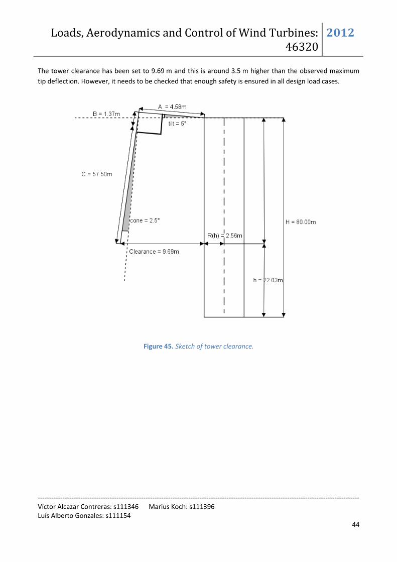
The tower clearance has been set to 9.69 m and this is around 3.5 m higher than the observed maximum
tip deflection. However, it needs to be checked that enough safety is ensured in all design load cases.
Figure 45. Sketch of tower clearance.
Loads, Aerodynamics and Control of Wind Turbines: 46320
2012
----------------------------------------------------------------------------------------------------------------------------------------------- Víctor Alcazar Contreras: s111346 Marius Koch: s111396 Luís Alberto Gonzales: s111154
45
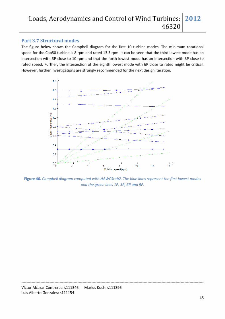
Part 3.7 Structural modes The figure below shows the Campbell diagram for the first 10 turbine modes. The minimum rotational
speed for the Cap50 turbine is 8 rpm and rated 13.3 rpm. It can be seen that the third lowest mode has an
intersection with 3P close to 10 rpm and that the forth lowest mode has an intersection with 3P close to
rated speed. Further, the intersection of the eighth lowest mode with 6P close to rated might be critical.
However, further investigations are strongly recommended for the next design iteration.
Figure 46. Campbell diagram computed with HAWCStab2. The blue lines represent the first lowest modes
and the green lines 1P, 3P, 6P and 9P.
Loads, Aerodynamics and Control of Wind Turbines: 46320
2012
----------------------------------------------------------------------------------------------------------------------------------------------- Víctor Alcazar Contreras: s111346 Marius Koch: s111396 Luís Alberto Gonzales: s111154
46
Part 4: Implementation of Risø basic PI controller In this section the implementation of the Risø basic PI controller is described.
Part 4.1: Setting of control parameters In this section the controller settings are described.
A constant torque control instead of a constant power control has been chosen because in the design
process there were problems with drive train vibrations and in order to narrow the problem it was assumed
that constant torque is more appropriate. Further, it is assumed that constant torque reduces the drive
train loads. However, in order to obtain a more stable power output it is recommended to investigate
constant power control in a next design iteration.
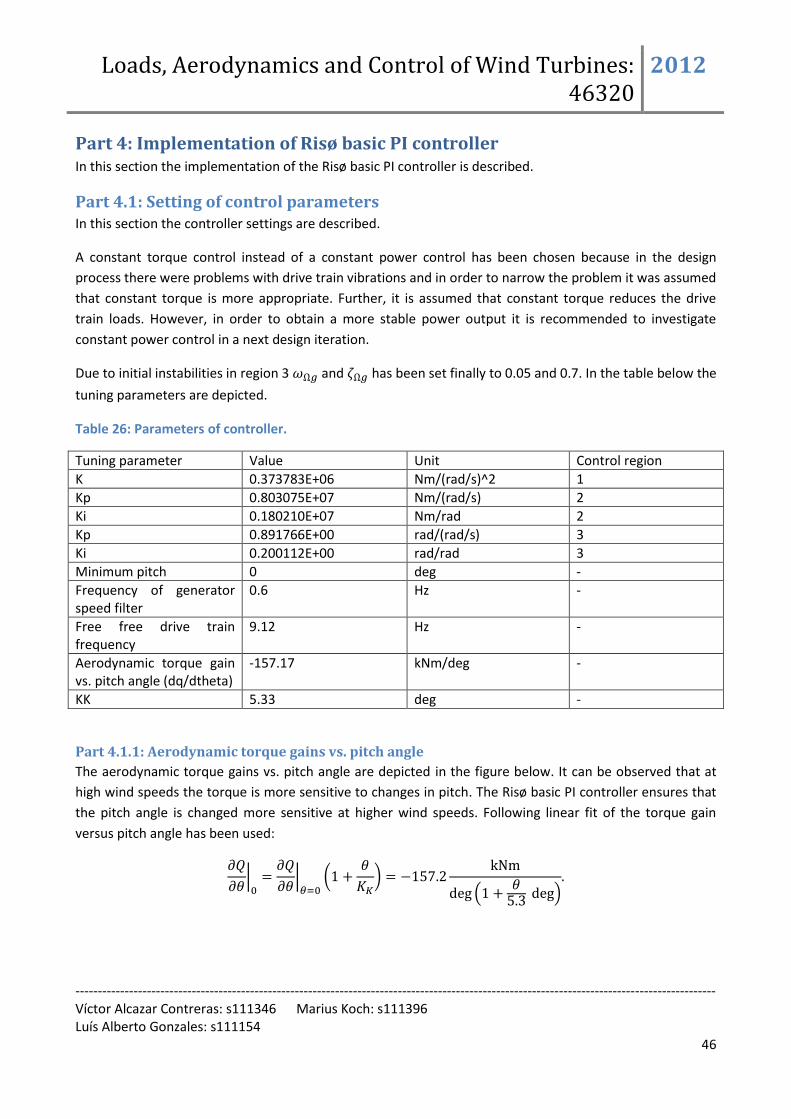
Due to initial instabilities in region 3 and has been set finally to 0.05 and 0.7. In the table below the
tuning parameters are depicted.
Table 26: Parameters of controller.
Tuning parameter Value Unit Control region
K 0.373783E+06 Nm/(rad/s)^2 1
Kp 0.803075E+07 Nm/(rad/s) 2
Ki 0.180210E+07 Nm/rad 2
Kp 0.891766E+00 rad/(rad/s) 3
Ki 0.200112E+00 rad/rad 3
Minimum pitch 0 deg -
Frequency of generator speed filter
0.6 Hz -
Free free drive train frequency
9.12 Hz -
Aerodynamic torque gain vs. pitch angle (dq/dtheta)
-157.17 kNm/deg -
KK 5.33 deg -
Part 4.1.1: Aerodynamic torque gains vs. pitch angle
The aerodynamic torque gains vs. pitch angle are depicted in the figure below. It can be observed that at
high wind speeds the torque is more sensitive to changes in pitch. The Risø basic PI controller ensures that
the pitch angle is changed more sensitive at higher wind speeds. Following linear fit of the torque gain
versus pitch angle has been used:

Loads, Aerodynamics and Control of Wind Turbines: 46320
2012
----------------------------------------------------------------------------------------------------------------------------------------------- Víctor Alcazar Contreras: s111346 Marius Koch: s111396 Luís Alberto Gonzales: s111154
47
Figure 47. Aerodynamic torque gain versus pitch angle including the linear fit to these gains.
Part 4.1.2: Free free drive train frequency
With HAWCStab2 the free free drive train frequency has been computed and a value of 9.12 Hz has been
obtained. This is a relatively high value. For the Cap50 turbine the ratio of the rotor and generator inertia
on the low speed shaft is much higher than for most turbines:
and therefore it can be assumed that the free free drive train mode is rather a fixed (rotor) free (generator)
mode as shown in the following equations:
where is the shaft length, the shear modulus of the shaft and torsional stiffness or polar moment of
inertia of the shaft.
If it can be estimated that:
Loads, Aerodynamics and Control of Wind Turbines: 46320
2012
----------------------------------------------------------------------------------------------------------------------------------------------- Víctor Alcazar Contreras: s111346 Marius Koch: s111396 Luís Alberto Gonzales: s111154
48
Attempts have been carried out to decrease the free free drive train frequency by decreasing the torsional
shaft stiffness. The flexible shaft configuration caused instabilities and therefore the stiff version has been
chosen. However, the shaft design shall be content of a further design iteration.
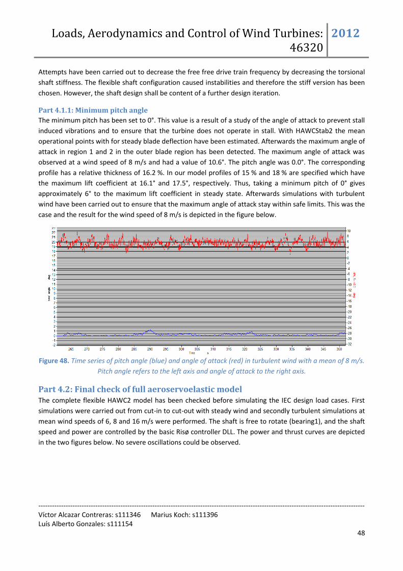
Part 4.1.1: Minimum pitch angle
The minimum pitch has been set to 0°. This value is a result of a study of the angle of attack to prevent stall
induced vibrations and to ensure that the turbine does not operate in stall. With HAWCStab2 the mean
operational points with for steady blade deflection have been estimated. Afterwards the maximum angle of
attack in region 1 and 2 in the outer blade region has been detected. The maximum angle of attack was
observed at a wind speed of 8 m/s and had a value of 10.6°. The pitch angle was 0.0°. The corresponding
profile has a relative thickness of 16.2 %. In our model profiles of 15 % and 18 % are specified which have
the maximum lift coefficient at 16.1° and 17.5°, respectively. Thus, taking a minimum pitch of 0° gives
approximately 6° to the maximum lift coefficient in steady state. Afterwards simulations with turbulent
wind have been carried out to ensure that the maximum angle of attack stay within safe limits. This was the
case and the result for the wind speed of 8 m/s is depicted in the figure below.
Figure 48. Time series of pitch angle (blue) and angle of attack (red) in turbulent wind with a mean of 8 m/s.
Pitch angle refers to the left axis and angle of attack to the right axis.
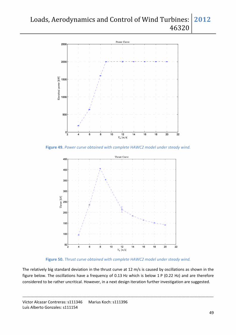
Part 4.2: Final check of full aeroservoelastic model The complete flexible HAWC2 model has been checked before simulating the IEC design load cases. First
simulations were carried out from cut-in to cut-out with steady wind and secondly turbulent simulations at
mean wind speeds of 6, 8 and 16 m/s were performed. The shaft is free to rotate (bearing1), and the shaft
speed and power are controlled by the basic Risø controller DLL. The power and thrust curves are depicted
in the two figures below. No severe oscillations could be observed.
Loads, Aerodynamics and Control of Wind Turbines: 46320
2012
----------------------------------------------------------------------------------------------------------------------------------------------- Víctor Alcazar Contreras: s111346 Marius Koch: s111396 Luís Alberto Gonzales: s111154
49
Figure 49. Power curve obtained with complete HAWC2 model under steady wind.
Figure 50. Thrust curve obtained with complete HAWC2 model under steady wind.
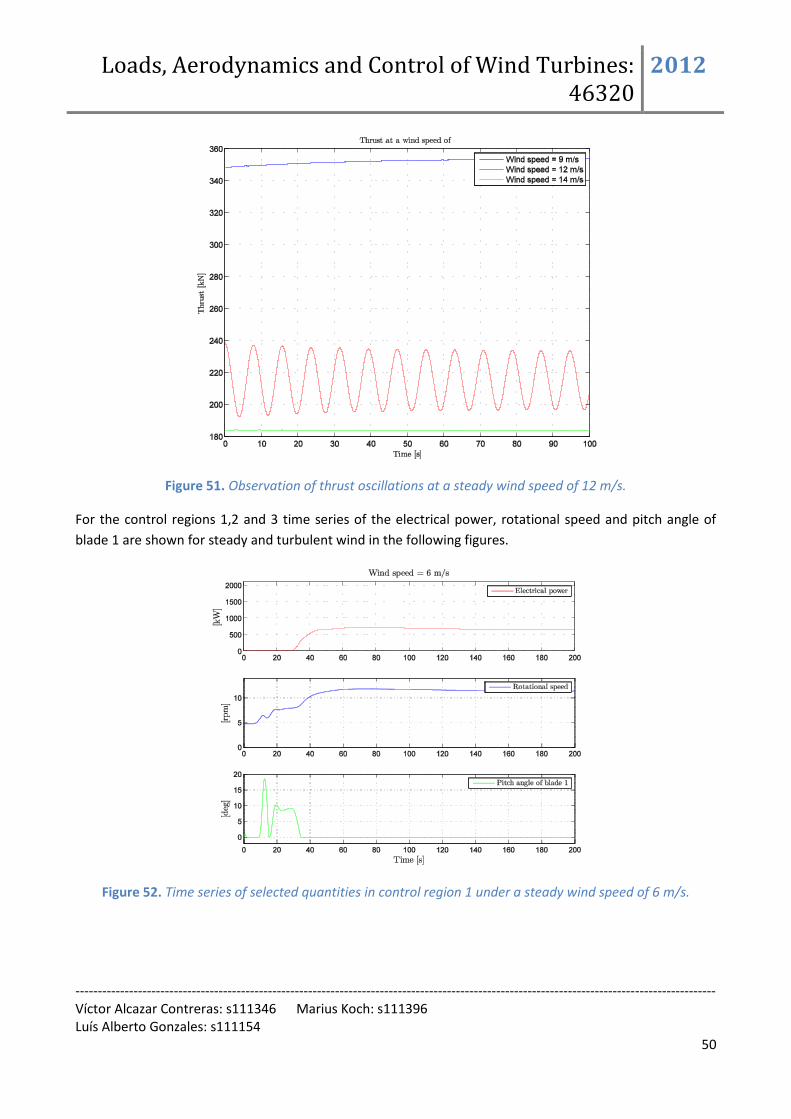
The relatively big standard deviation in the thrust curve at 12 m/s is caused by oscillations as shown in the
figure below. The oscillations have a frequency of 0.13 Hz which is below 1 P (0.22 Hz) and are therefore
considered to be rather uncritical. However, in a next design iteration further investigation are suggested.
Loads, Aerodynamics and Control of Wind Turbines: 46320
2012
----------------------------------------------------------------------------------------------------------------------------------------------- Víctor Alcazar Contreras: s111346 Marius Koch: s111396 Luís Alberto Gonzales: s111154
50
Figure 51. Observation of thrust oscillations at a steady wind speed of 12 m/s.
For the control regions 1,2 and 3 time series of the electrical power, rotational speed and pitch angle of
blade 1 are shown for steady and turbulent wind in the following figures.
Figure 52. Time series of selected quantities in control region 1 under a steady wind speed of 6 m/s.

Loads, Aerodynamics and Control of Wind Turbines: 46320
2012
----------------------------------------------------------------------------------------------------------------------------------------------- Víctor Alcazar Contreras: s111346 Marius Koch: s111396 Luís Alberto Gonzales: s111154
51
Figure 53. Time series of selected quantities in control region 2 under a steady wind speed of 8 m/s.
Figure 54. Time series of selected quantities in control region 3 under a steady wind speed of 16 m/s.

Loads, Aerodynamics and Control of Wind Turbines: 46320
2012
----------------------------------------------------------------------------------------------------------------------------------------------- Víctor Alcazar Contreras: s111346 Marius Koch: s111396 Luís Alberto Gonzales: s111154
52
Figure 55. Time series of selected quantities in control region 1 under turbulent wind speed with a mean of
6 m/s.
Figure 56. Time series of selected quantities in control region 2 under turbulent wind speed with a mean of
8 m/s.

Loads, Aerodynamics and Control of Wind Turbines: 46320
2012
----------------------------------------------------------------------------------------------------------------------------------------------- Víctor Alcazar Contreras: s111346 Marius Koch: s111396 Luís Alberto Gonzales: s111154
53
Figure 57. Time series of selected quantities in control region 3 under turbulent wind speed with a mean of
16 m/s.
Part 5: Aero-elastic Analysis For this work a reduced set of Design Load Cases (DLC) according to IEC 61400-1 Ed.3 has been simulated
with HAWC2. In this section a brief description of the considered DLCs is provided and the fatigue and
ultimate loads are presented. Further, the power curve is depicted and the Annual Energy Production (AEP)
and the capacity factor are calculated.
Part 5.1: Design Load Cases In this section a description of the considered DLCs can be found. For further details it is referred to IEC
61400-1 Ed.3. For all simulations the first 5 s are chopped of as required by IEC. It shall be noted that for
DLC 1.1/1.2, 1.3 and 6.1 six 10 min realizations are required by IEC but in this work a reduced amount of
simulations has been carried out as stated in the tables below.
Part 5.1.1: Design load case 1.1/1.2
Type of analysis Ultimate/ fatigue loads
Turbine state Power production
Wind condition NTM V_in < V_hub < V_out
Turbulence model Mann
Partial safety factor */1.25
Yaw misalignment -10°,0°,10°
10 min realizations per wind speed 3

Loads, Aerodynamics and Control of Wind Turbines: 46320
2012
----------------------------------------------------------------------------------------------------------------------------------------------- Víctor Alcazar Contreras: s111346 Marius Koch: s111396 Luís Alberto Gonzales: s111154
54
It shall be noted that this DLC is used to carry out the load extrapolation as described in IEC 61400-1 Ed.3.
In case the extrapolated loads are higher than from DLC 1.3 the c parameter in equation 19 in IEC 61400-1
Ed.3 must be increased until DLC 1.3 gives higher loads.
Part 5.1.2: Design load case 1.3
Type of analysis Ultimate loads
Turbine state Power production
Wind condition ETM V_in < V_hub < V_out
Turbulence model Mann
Partial safety factor N = 1.35
Yaw misalignment 0°
10 min realizations per wind speed 3
It shall be noted that if the extrapolated loads from DLC 1.1 are higher than from DLC 1.3 the c parameter
in equation 19 in IEC 61400-1 Ed.3 must be increased until DLC 1.3 gives higher loads.
Part 5.1.3: Design load case 6.1
Type of analysis Ultimate loads
Turbine state Parked (idling)
Wind condition EWM V_ref = 37.5
Turbulence model Mann
Partial safety factor N = 1.35
Yaw misalignment -90°,-8°,8°,90°
10 min realizations per wind speed and yaw misalignment
1
Since the turbine is parked, more yaw misalignments shall be considered in a more advanced study.
Part 5.2: Fatigue and extreme loads under normal production.
A) Equivalent Fatigue Loads
The HAWC2 results file for the turbine on normal turbulence operation (NTM) case is extracted for the
fatigue post-process. For each wind speed and yaw case, the fatigue equivalent loads are to be calculated
and represented.
Briefly, the calculation procedure is described: First, the time series from the tower longitudinal and lateral
bending moments, the shaft bending moments, the yaw moment, and the blade flap/edgewise bending
moments waveforms go through these steps:
Compute a peak version of the signal, which only contains the maximums and minimums
Perform a rainflow counting to get the load ranges their corresponding number of cycles.
Add all of the contributions in order to calculate the equivalent load.
(5.1)

Loads, Aerodynamics and Control of Wind Turbines: 46320
2012
----------------------------------------------------------------------------------------------------------------------------------------------- Víctor Alcazar Contreras: s111346 Marius Koch: s111396 Luís Alberto Gonzales: s111154
55
Where:
Si : is the load range
No: 1 per second samples in 10 min (600), this is to calculate the 1Hz equivalent fatigue load.
m: is the material property constant (for glass fiber m = 12)
So: is the equivalent fatigue load.
The following results are presented.
Figure 58. Fatigue analysis Flap/Edge-wise bending moments.

Loads, Aerodynamics and Control of Wind Turbines: 46320
2012
----------------------------------------------------------------------------------------------------------------------------------------------- Víctor Alcazar Contreras: s111346 Marius Koch: s111396 Luís Alberto Gonzales: s111154
56
Figure 59. Fatigue analysis Shaft bending moments.
Figure 60. Fatigue analysis Tower bending moments

Loads, Aerodynamics and Control of Wind Turbines: 46320
2012
----------------------------------------------------------------------------------------------------------------------------------------------- Víctor Alcazar Contreras: s111346 Marius Koch: s111396 Luís Alberto Gonzales: s111154
57
Figure 61. Fatigue analysis Yaw moment
Finally worth to mention the cases 18 and 20 m/s have been removed from the fitting. Due to the unstable
behavior both show. To demonstrate this, the blade edgewise bending moment, (parameter relevant as
well for the extreme extrapolation) is shown in a stable and unstable case below. It has been chosen as an
example because it is known the Mb edgewise should be fairly constant in size (it is mainly driven by the
rotor weight) no matter what is the wind speed is.
Figure 62. Time series of Mxb1 edge, V=16 m/s.
Figure 63. Time series of Mxb1 edge, V=20 m/s.
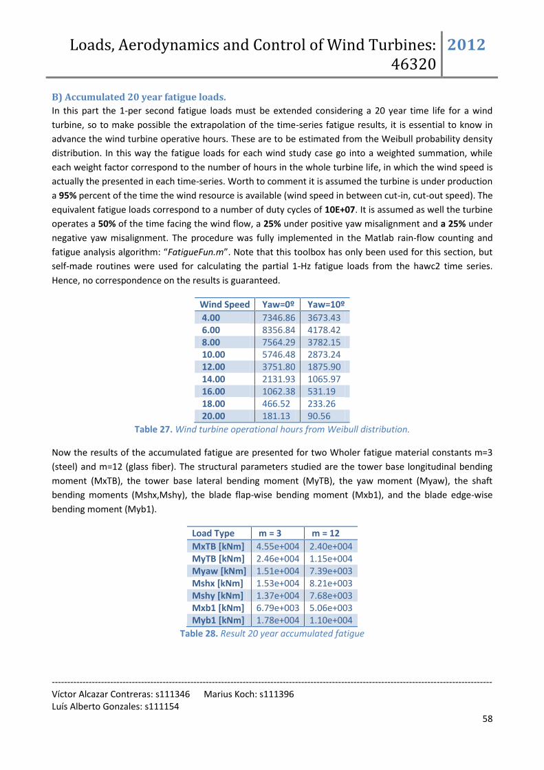
Loads, Aerodynamics and Control of Wind Turbines: 46320
2012
----------------------------------------------------------------------------------------------------------------------------------------------- Víctor Alcazar Contreras: s111346 Marius Koch: s111396 Luís Alberto Gonzales: s111154
58
B) Accumulated 20 year fatigue loads.
In this part the 1-per second fatigue loads must be extended considering a 20 year time life for a wind
turbine, so to make possible the extrapolation of the time-series fatigue results, it is essential to know in
advance the wind turbine operative hours. These are to be estimated from the Weibull probability density
distribution. In this way the fatigue loads for each wind study case go into a weighted summation, while
each weight factor correspond to the number of hours in the whole turbine life, in which the wind speed is
actually the presented in each time-series. Worth to comment it is assumed the turbine is under production
a 95% percent of the time the wind resource is available (wind speed in between cut-in, cut-out speed). The
equivalent fatigue loads correspond to a number of duty cycles of 10E+07. It is assumed as well the turbine
operates a 50% of the time facing the wind flow, a 25% under positive yaw misalignment and a 25% under
negative yaw misalignment. The procedure was fully implemented in the Matlab rain-flow counting and
fatigue analysis algorithm: “FatigueFun.m”. Note that this toolbox has only been used for this section, but
self-made routines were used for calculating the partial 1-Hz fatigue loads from the hawc2 time series.
Hence, no correspondence on the results is guaranteed.
Wind Speed Yaw=0º Yaw=10º
4.00 7346.86 3673.43 6.00 8356.84 4178.42 8.00 7564.29 3782.15 10.00 5746.48 2873.24 12.00 3751.80 1875.90 14.00 2131.93 1065.97 16.00 1062.38 531.19 18.00 466.52 233.26 20.00 181.13 90.56
Table 27. Wind turbine operational hours from Weibull distribution.
Now the results of the accumulated fatigue are presented for two Wholer fatigue material constants m=3
(steel) and m=12 (glass fiber). The structural parameters studied are the tower base longitudinal bending
moment (MxTB), the tower base lateral bending moment (MyTB), the yaw moment (Myaw), the shaft
bending moments (Mshx,Mshy), the blade flap-wise bending moment (Mxb1), and the blade edge-wise
bending moment (Myb1).
Load Type m = 3 m = 12
MxTB [kNm] 4.55e+004 2.40e+004 MyTB [kNm] 2.46e+004 1.15e+004 Myaw [kNm] 1.51e+004 7.39e+003 Mshx [kNm] 1.53e+004 8.21e+003 Mshy [kNm] 1.37e+004 7.68e+003 Mxb1 [kNm] 6.79e+003 5.06e+003 Myb1 [kNm] 1.78e+004 1.10e+004
Table 28. Result 20 year accumulated fatigue

Loads, Aerodynamics and Control of Wind Turbines: 46320
2012
----------------------------------------------------------------------------------------------------------------------------------------------- Víctor Alcazar Contreras: s111346 Marius Koch: s111396 Luís Alberto Gonzales: s111154
59
C) Extreme load extrapolation
The steps are described in the standard IEC 61400-1. To summarize them briefly, the time series of each
structural parameter (either bending moment or the tip deflection) is extracted from the Hawc2 result file
into Matlab. The peak-over-threshold method is used to calculate the extreme load extrapolation with the
following steps.
First, the mean and standard deviation of the structural measurement is calculated, and from these values,
the threshold is located at
(5.1)
If the curve minimum is higher in magnitude than the maximum, this last value will be considered the
extreme from this point, and the curve will be mirrored. A subroutine is responsible of extracting the peaks
over this threshold by chopping the time series in arrays of values over the limit, and calculating the
maximum. In the following picture this process is shown for the tip deflection at V=10m/s, for the yaw case
of -10º.
Figure 64. Tip deflection time series V=10 m/s Yaw=10º.
Since 3 yaw cases are studied, the peaks of each are extracted and stored, as well as the maximum load of
the three recordings (ultimate load). Now the probability of having a higher load is derived for each peak,
since
(5.2)
This probability curve can be fitted to a Gumbel distribution, its parameters are found by calculating with a
linear poly-fitting on the logarithm of the signal.
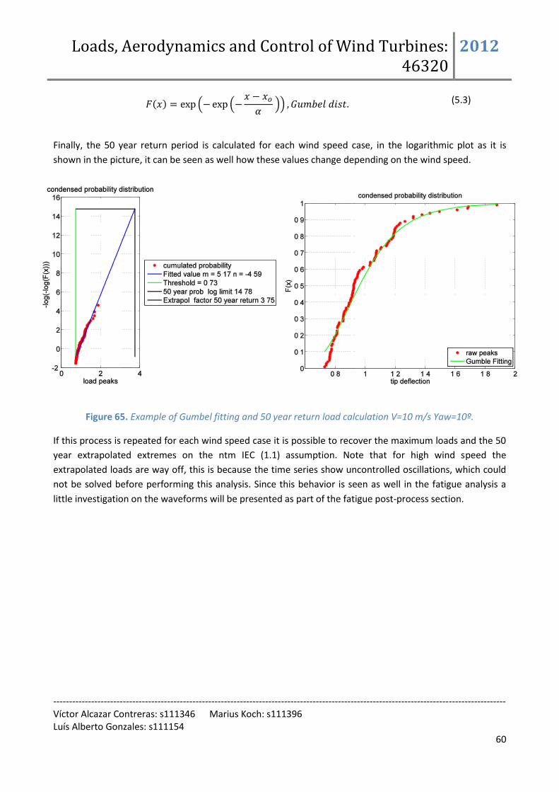
Loads, Aerodynamics and Control of Wind Turbines: 46320
2012
----------------------------------------------------------------------------------------------------------------------------------------------- Víctor Alcazar Contreras: s111346 Marius Koch: s111396 Luís Alberto Gonzales: s111154
60
(5.3)
Finally, the 50 year return period is calculated for each wind speed case, in the logarithmic plot as it is
shown in the picture, it can be seen as well how these values change depending on the wind speed.
Figure 65. Example of Gumbel fitting and 50 year return load calculation V=10 m/s Yaw=10º.
If this process is repeated for each wind speed case it is possible to recover the maximum loads and the 50
year extrapolated extremes on the ntm IEC (1.1) assumption. Note that for high wind speed the
extrapolated loads are way off, this is because the time series show uncontrolled oscillations, which could
not be solved before performing this analysis. Since this behavior is seen as well in the fatigue analysis a
little investigation on the waveforms will be presented as part of the fatigue post-process section.

Loads, Aerodynamics and Control of Wind Turbines: 46320
2012
----------------------------------------------------------------------------------------------------------------------------------------------- Víctor Alcazar Contreras: s111346 Marius Koch: s111396 Luís Alberto Gonzales: s111154
61
Figure 66. Maximum and extreme load extrapolated results from NTM (1.1) Yaw moment and Tower base
longitudinal moment.
Figure 67. Maximum and extreme load extrapolated results from NTM (1.1) Blade flap-wise bending
moment and blade tip deflection.
Finally worth to mention in the Standard it is recommended to give the overall extreme extrapolated load
with a single value, and not with a discrete sequence of wind speed tests. Hence, it was attempted to make
a weighted summation of each probability Gumble distribution, considering the probability of having a
certain wind speed (Which is represented by the Weibull distribution). In this following way:

Loads, Aerodynamics and Control of Wind Turbines: 46320
2012
----------------------------------------------------------------------------------------------------------------------------------------------- Víctor Alcazar Contreras: s111346 Marius Koch: s111396 Luís Alberto Gonzales: s111154
62
(5.4)
With ni the average number of peaks per wind study case, Fv the corresponding Gumbel-fitted probability,
and p(Vi) coming from the Weibull distribution. Unfortunately, due to the uncertainty on high wind speed,
it was not possible to achieve an accurate prediction of the extreme, since these errors heavily affect the
accumulated probability distribution.
Figure 68. Accumulated probability load distribution, tip deflection example.
By comparing both figures (partial and accumulated) for the tip deflection sample, it is clear the
accumulated value (around 8 m) is the same as the value for 50 year return deflection at Vs=20 m/s. So to
do properly this calculation it would be required: First, to remove the unstable study cases, and to ensure
the weighting factors (coming from the Weibull dist.) integral is 1, (which as it is shown in the figure is not
the case).

Loads, Aerodynamics and Control of Wind Turbines: 46320
2012
----------------------------------------------------------------------------------------------------------------------------------------------- Víctor Alcazar Contreras: s111346 Marius Koch: s111396 Luís Alberto Gonzales: s111154
63
D) Comparison with ETM maximum loads.
In this part the purpose is to calculate the maximum peaks. The time series which are chosen come from
the IEC standard DLC ETM (1.3). This study line is the extreme turbulence mode. The maximum values must
be compared with the output of the section before (extrapolated maxima, from normal operation) to check
the former ones are not bigger, if this is the case, the ETM simulation should be repeated with increased
turbulence intensity. As it can be seen in the figure this is the case, although that has not been performed
due to the lack of available time. Note that for increased wind speed the ETM simulations are still stable, so
V=[18-20]m/s results cannot be compared with the 50 year extrapolated loads.
Figure 69. Comparison between ETM (1.3) and NTM (1.1) Ultimate loads Yaw moment and Tower base
longitudinal moment.
Figure 70. Comparison between ETM (1.3) and NTM (1.1) Ultimate loads Blade flap-wise bending moment
and blade tip deflection.
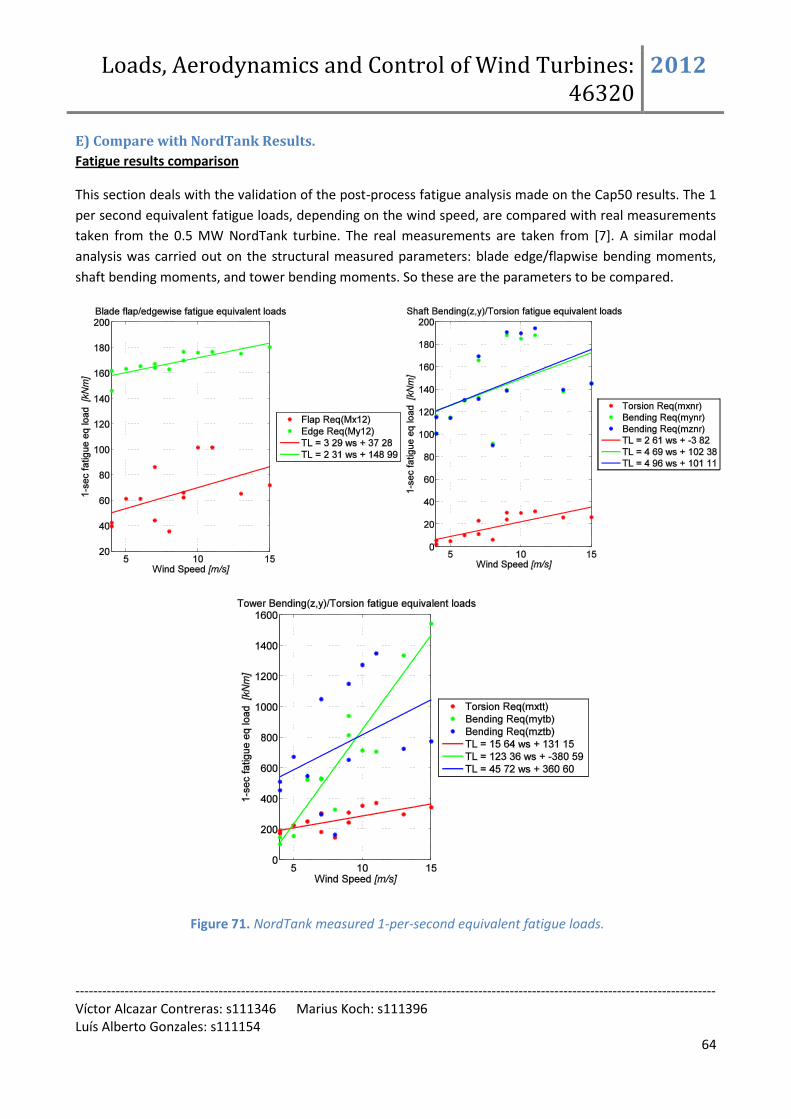
Loads, Aerodynamics and Control of Wind Turbines: 46320
2012
----------------------------------------------------------------------------------------------------------------------------------------------- Víctor Alcazar Contreras: s111346 Marius Koch: s111396 Luís Alberto Gonzales: s111154
64
E) Compare with NordTank Results.
Fatigue results comparison
This section deals with the validation of the post-process fatigue analysis made on the Cap50 results. The 1
per second equivalent fatigue loads, depending on the wind speed, are compared with real measurements
taken from the 0.5 MW NordTank turbine. The real measurements are taken from [7]. A similar modal
analysis was carried out on the structural measured parameters: blade edge/flapwise bending moments,
shaft bending moments, and tower bending moments. So these are the parameters to be compared.
Figure 71. NordTank measured 1-per-second equivalent fatigue loads.
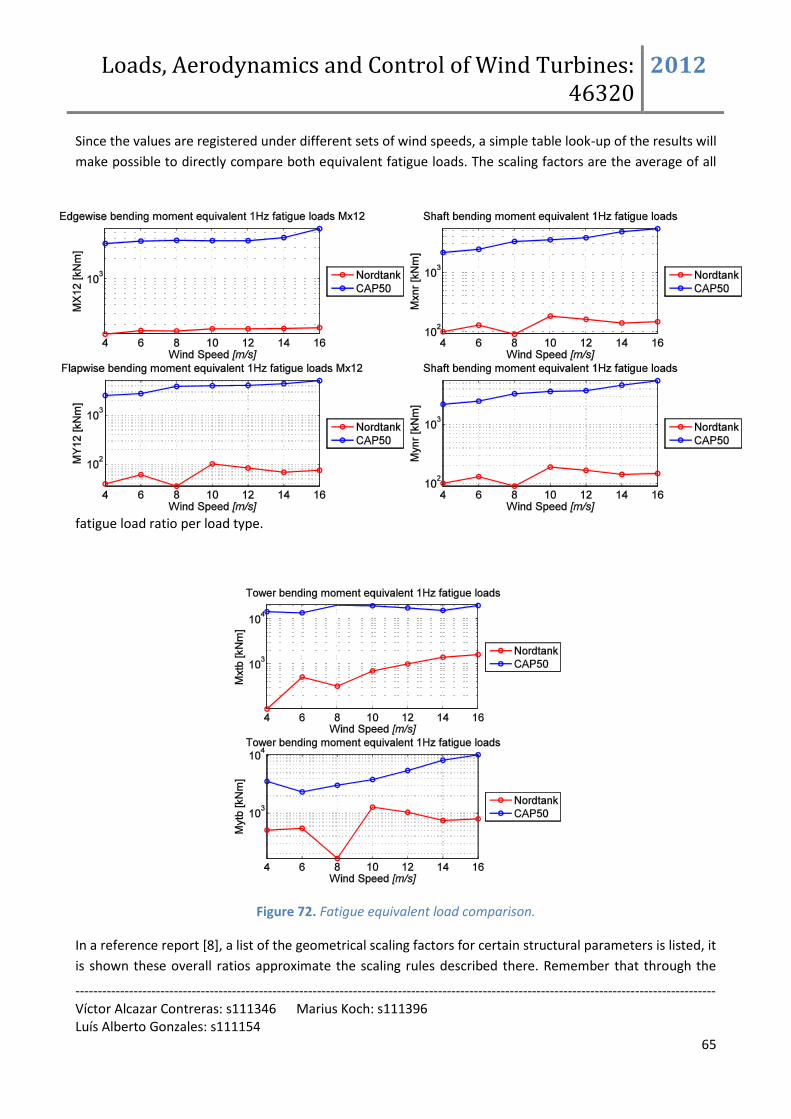
Loads, Aerodynamics and Control of Wind Turbines: 46320
2012
----------------------------------------------------------------------------------------------------------------------------------------------- Víctor Alcazar Contreras: s111346 Marius Koch: s111396 Luís Alberto Gonzales: s111154
65
Since the values are registered under different sets of wind speeds, a simple table look-up of the results will
make possible to directly compare both equivalent fatigue loads. The scaling factors are the average of all
fatigue load ratio per load type.
Figure 72. Fatigue equivalent load comparison.
In a reference report [8], a list of the geometrical scaling factors for certain structural parameters is listed, it
is shown these overall ratios approximate the scaling rules described there. Remember that through the

Loads, Aerodynamics and Control of Wind Turbines: 46320
2012
----------------------------------------------------------------------------------------------------------------------------------------------- Víctor Alcazar Contreras: s111346 Marius Koch: s111396 Luís Alberto Gonzales: s111154
66
project, both similarity rules for power production and geometry of the rotor have been used. It was
decided to use the geometrical proportion:
Ratio power (2MW/0.5MW)=4
Ratio rotor diameter (57.5m/20.5m)=2.8
Table 29. Scaling rules
FATIGUE 1-hz Analysis Scaling reference rule Overall Factor
Blade, Root Bending Moment-X 24.0261 closer to geometry ratio Blade, Root Bending Moment-Y 62.8251 closer to power ratio Shaft, Bending Mom - X 27.5396 Below ref. Shaft, Bending Mom - Y 27.0267 Below ref. Tower, Bending Mom - X 42.8315 closer to power ratio Tower, Bending Mom - Y 8.8427 Below ref.
Table 30. Comparison with Nordtank turbine, scaling factors
Extreme results comparison
Since it is available Hawc2 result files from the NordTank, these will be used to compute the return loads
and the ultimate loads, for the same structural parameters as it was done for Cap50. The purpose is to
compare both, and calculate scaling factors again to cross-reference them with the Chaviaropoulos report
[8]. For such task, the design ultimate loads (the maxima between 50 years extrapolated NTM and ultimate
ETM loads) are to be calculated. These are shown in figures below, for both NTK and CAP50.
Figure 73. Design ultimate loads comparison between NTK and Cap 50. Tower base bending moment and
Yaw moment
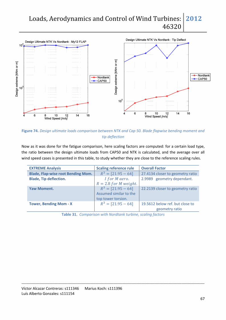
Loads, Aerodynamics and Control of Wind Turbines: 46320
2012
----------------------------------------------------------------------------------------------------------------------------------------------- Víctor Alcazar Contreras: s111346 Marius Koch: s111396 Luís Alberto Gonzales: s111154
67
Figure 74. Design ultimate loads comparison between NTK and Cap 50. Blade flapwise bending moment and
tip deflection
Now as it was done for the fatigue comparison, here scaling factors are computed: for a certain load type,
the ratio between the design ultimate loads from CAP50 and NTK is calculated, and the average over all
wind speed cases is presented in this table, to study whether they are close to the reference scaling rules.
EXTREME Analysis Scaling reference rule Overall Factor
Blade, Flap-wise root Bending Mom. 27.4134 closer to geometry ratio Blade, Tip deflection.
2.9989 geometry dependant.
Yaw Moment. Assumed similar to the top tower torsion.
22.2139 closer to geometry ratio
Tower, Bending Mom - X 19.5612 below ref. but close to geometry ratio
Table 31. Comparison with Nordtank turbine, scaling factors

Loads, Aerodynamics and Control of Wind Turbines: 46320
2012
----------------------------------------------------------------------------------------------------------------------------------------------- Víctor Alcazar Contreras: s111346 Marius Koch: s111396 Luís Alberto Gonzales: s111154
68
Part 5.3: Power and thrust curves The power and thrust curves have been computed based on the simulation results from DLC 1.1 and all
three yaw misalignments. The wind speed corresponding to a power or thrust level is the mean of the
turbulent wind speed time series. The results are presented in the figures below. It can be seen that the
mean wind speed is above rated for the last two simulations and therefore these results are disregarded in
the computation of the Annual Energy Production (AEP).
Figure 75. Power curve based on DLC 1.1 and all three yaw misalignments.
Figure 76. Thrust curve based on DLC 1.1 and all three yaw misalignments.

Loads, Aerodynamics and Control of Wind Turbines: 46320
2012
----------------------------------------------------------------------------------------------------------------------------------------------- Víctor Alcazar Contreras: s111346 Marius Koch: s111396 Luís Alberto Gonzales: s111154
69
Part 5.4: Annual Energy Production In this section the Annual Energy Production (AEP) is calculated based on the wind distribution suggested in
IEC 61400-1 Ed.3 for Vref = 37.5 m/s. The power curve has been computed based on the simulation results
from DLC 1.1 as described in the previous section.
The AEP can be written as:
The capacity factor can be calculated as follows:
It can be seen that the main design criterion of the Cap50 turbine, to obtain a capacity factor above
50 %, is archived.

Loads, Aerodynamics and Control of Wind Turbines: 46320
2012
----------------------------------------------------------------------------------------------------------------------------------------------- Víctor Alcazar Contreras: s111346 Marius Koch: s111396 Luís Alberto Gonzales: s111154
70
Conclusions
Suggestions for further iterations, limitations of the current design:
Overall turbine: The htc model must be fixed first to analyze the sources of instability in the structural root
blade bending moments, and the fatigue and extreme load post-process should be repeated again to check
the actual values of the ultimate design loads. In this report, they are performed based partially on
incomplete results, only to show that the process has been tried.
Blades: to manipulate the section layout, and to draw the section thickness profiles towards the blade
flange. It has appeared uncontrolled edgewise root bending moment oscillations for high wind speeds. One
reason might be the blade cannot carry properly a gust even if high deflections are expected (it has been
implemented already a pre-bending). Hence, once the Hawc2 model is fixed a root optimization of the
blade must be done. Meaning, from the design load bending moments, the stresses and strains must be
recovered along the blade surface, the maximum stresses are to be localized, and compensated with more
robust airfoil section geometry.
Tower: Many difficulties have been occurred to decide the main tower geometry, the tower top may be to
thin. Hence, uncontrolled torsion or concentrated stresses may arise if the turbine is tilted or yawed
unexpectedly. The tower might be over-dimensioned for the power produced, due to the very large rotor.
Further costs considerations on tower manufacture/erection must be addressed in the next iteration.
Another issue is that a fine site exploration could show less ground influence and less wind shear, in this
case, perhaps the tower height could be reduced. Remember for such project no need of going up in height
for higher wind speeds (and higher loads on the whole turbine) is recommended, since the turbine is
capable to produce rated power at very low wind velocity.
Shaft: The main issue was to merge design constraints coming from different parts of the turbine at the
same time. The big rotor demanded a stiff shaft in bending, which was not totally well defined. The main
bearing position should be decided, and the step in bending stiffness should be better settled. Secondly,
the generator inertia was very tiny compared with the inertia from a machine proportional to such shaft
(4MW generator). This made very hard the controller routine to handle such big free-free drive-train
frequency. Hence, the controller would like a more flexible shaft in torsion. But the real question is whether
is necessary such stiff shaft. The blades are big in size, but very light. Perhaps a more flexible shaft (in
torsion) would be capable to handle the aerodynamic less severe loading on the rotor due to the low wind
speed conditions of the site. If this is the case, it would be possible to reduce costs in shaft and nacelle
mass, with a more robust controller strategy.

Loads, Aerodynamics and Control of Wind Turbines: 46320
2012
----------------------------------------------------------------------------------------------------------------------------------------------- Víctor Alcazar Contreras: s111346 Marius Koch: s111396 Luís Alberto Gonzales: s111154
71
References: [1] www.hawc2.dk
[2] Scaling spreadsheet: Upscaled_Turbine
[3] Bak C., "Aerodynamic design of wind turbine rotors", Risø-I-3202(EN), Risø DTU, September 2011
[4] Bak C., "Aerodynamic Rotor Design", Technical University of Denmark, 2012
[5] Bertagnolio F., Sørensen N, Johansen J. and Figlsang P., "Wind Turbine Airfoil Catalogue", Risø-R-
1280(EN), Risø National Laboratory, Roskilde, Denmark, August 2001.
[6] Wind turbines - Part1: Design requirements (IEC 61400 -1 Ed. 3). IEC, Third edition, 2005 - 8
[7] 46400. Wind turbine measurement technique documentation. DTU course.
[8] SIMILARITY RULES FOR W/T UP-SCALING. by P.K. Chaviaropoulos
[9] Vermeer L.J., Sørensen J.N., Crespo A., "Wind turbine wake aerodynamics", Progress in Aerospace
Sciences, 2003
[10] Burton T., Sharpe D., Jenkins N and Bossanyi E., "Wind Energy Handbook", John Wiley & sons, LTD,
2001
[11] http://www.ductile.org/didata/Section3/3part1.htm

Loads, Aerodynamics and Control of Wind Turbines: 46320
2012
----------------------------------------------------------------------------------------------------------------------------------------------- Víctor Alcazar Contreras: s111346 Marius Koch: s111396 Luís Alberto Gonzales: s111154
72
Appendix:
A.1 Structural mesh output from becas
Root section n.2. R= 0.8193 m
Structural airfoil n.28 R= 19.5212 m

Loads, Aerodynamics and Control of Wind Turbines: 46320
2012
----------------------------------------------------------------------------------------------------------------------------------------------- Víctor Alcazar Contreras: s111346 Marius Koch: s111396 Luís Alberto Gonzales: s111154
73
Aerodynamic airfoil n.54 R= 38.2231 m
Tip airfoil n.80 R= 56.9250 m

Loads, Aerodynamics and Control of Wind Turbines: 46320
2012
----------------------------------------------------------------------------------------------------------------------------------------------- Víctor Alcazar Contreras: s111346 Marius Koch: s111396 Luís Alberto Gonzales: s111154
74