Aerodynamics of a Cambered Airfoil · Group 1 - December 13, 2017 Jackson Kistler, ∗ Noah...

ASEN 2002Aerodynamics of a Cambered Airfoil

Experimental LabGroup 1 - December 13, 2017

Jackson Kistler, ∗ Noah Francis, † Nathan Herr, ‡ Jarrod Puseman, §

University of Colorado - Boulder

The main premise of this experiment was to relate the lift and drag to the differentangles of attack of a cambered airfoil. This was done experimentally using a Clark Y-14airfoil model with 19 surface pressure ports in the ITLL wind tunnel. The differentialpressure between the ports was found and used to find the Coefficient of Pressure. Thesewere then used to find the axial and perpendicular coefficients, which are easily convertedinto the Coefficient of Drag and the Coefficient of Lift. These coefficients were calculatedfor each of the 32 angles that the section of Aerodynamics measured and graphs weregenerated to match and compare to the graphs in the NACA report 628 from 1938. Thegoal was to find the maximum lift that this airfoil can produce, if it has an angle of attackwhere the drag and coefficient of pressure are minimum. All of this data was run for higherairspeeds to see how the graphs change with higher Reynolds and Mach numbers. Thesedata and the analysis are presented here.

Nomenclature

α = Angle of Attack [deg]a = Axial Force [N]Ca = Coefficient of the Axial ForceCD = Coefficient of Pressure DragcD = Coefficient of Sectional Pressure DragCL = Coefficient of LiftcL = Coefficient of Sectional LiftCn = Coefficient of the Normal ForceCP = Coefficient of PressureD = Drag [N]L = Lift [N]n = Normal Force [N]

∗106270608†105248469‡106545930§104003252

ASEN 2002 Section 014 1 of 12 Fall 2017

I. Introduction

Airfoils, the fundamental cross-sectional geometry in an aircrafts wing, are critical to the production ofdrag and lift on aerodynamic vehicles. Because the distribution of pressure and shear-stress on the surfacesof a vehicle make up all of the aerodynamic forces acting on that vehicle, quantifying and integrating thepressure distribution around the geometry of an airfoil leads to an understanding how lift and drag are createdon aerodynamic vehicles. For the purposes of this experiment, a cambered Clark Y-14 airfoil, instrumentedwith 19 flush mounted pressure taps around its surface, was mounted in a wind tunnel such that pressuredistribution on the surface could be measured for varying angles of attack and airspeed. In this lab, theaerodynamic performance of the airfoil is calculated by determining how pressure distribution varies withtime and angle of attack, by determining if there are indications of flow separation of the surface, and byfinding the largest change in pressure between an upper and lower surface. This performance is then analyzedto gain an understanding of how angle of attack affects lift and drag, and how the results compare to thoseproduced by NACA in 1938.

II. Experimental Setup and Measurement Techniques

For this experiment, the Clark Y-14 airfoil was mounted vertically in the wind tunnel on a rotating platesuch that the angle of attack could be adjusted between trials. Group 1 started the experiment with anangle of attack of -8 and an airspeed velocity of 9 meters per second. The velocity was then increased to 17meters per second and finally 34 meters per second at the same angle of attack. The group then brought thevelocity back to zero, opened up the test section, adjusted the angle of attack to zero, and resealed the testsection. This same process was repeated for angles of attack zero, eight, and 16◦. Special care was takento ensure that the velocity was raised gradually for the protection of the wind tunnel. This same procedurewas repeated by the other lab groups in order to account for all angles of attack between -15 and 16◦, at thesame three testing velocities. All data was recorded on the LabVIEW VI on the wind tunnel computer andsaved according to the given file naming convention.

III. Post-processing and Calculation of Force Coefficient

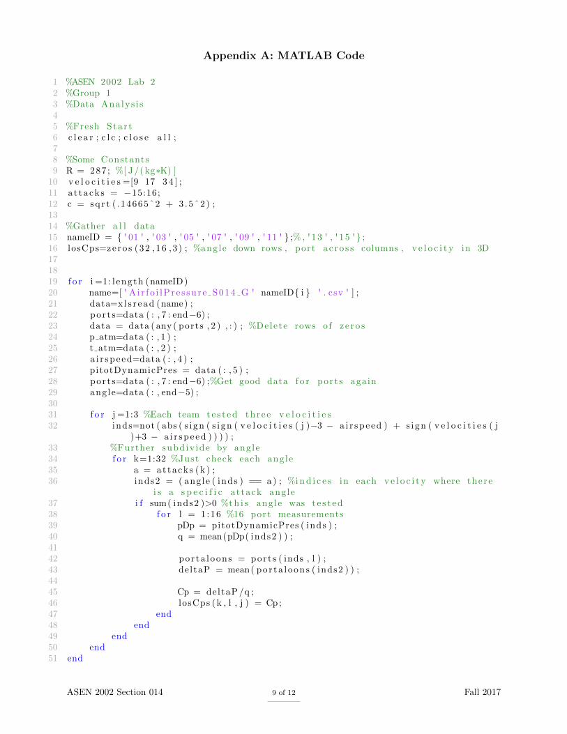
One major source of uncertainty in the calculation of the lift and pressure drag was the fact that only16 flush mounted pressure taps were used to collect data. The wing was outfitted with 19 such pressuretaps, but only 16 were used for the purposes of the experiment. Uncertainty could have been reduced ifmore pressure taps were utilized. The method used to compute the trailing edge pressure was to extrapolatepressure measurements from the top and bottom of the wing section to the trailing edge, and average theseextrapolations. While this method can provide a reasonable estimation of the pressure at the trailing edge,it is not as accurate as it would be if pressure at that point could be directly measured. The differentialpressures were then numerically integrated around the airfoil surface to find the net axial and normal forcesacting on the wing. From these forces the force coefficients and henceforth the lift and drag coefficients werederived.

IV. Airfoil Static Pressure Coefficient Distribution

The pressure coefficient versus normalized chord-wise position for several angles of attack is plotted inFig. 1. See how for large negative angles of attack, the Cp for the bottom of the foil is ”above” that of thetop surface of the foil. This means the airfoil is creating negative lift at these angles of attack. As the anglehits -5◦, the bottom surface Cp values start to go back ”below” the top surface as lift stops acting downwardon the foil. At 0◦, the Cp curve looks similar to the traditional example of the pressure coefficient curve.As the angle creeps into 5 and 10◦, the Cp values get larger in magnitude and the bottom surface starts tocontribute more lift.

The angles of attack measured by group 1 were -8, 0, 8, and 16◦. The pressure distributions at theseangles are plotted in Fig. 2. See that the pressure distributions are consistent with the trends set by therest of the class like in Fig. 1. At larger negative angles of attack, the lower surface distribution is abovethe upper surface, indicating a force downward on the wing. For 0 angle of attack, the profile looks likethe standard Cp distribution, and for the larger angles of attack, the Cp distributions for both surfaces tend


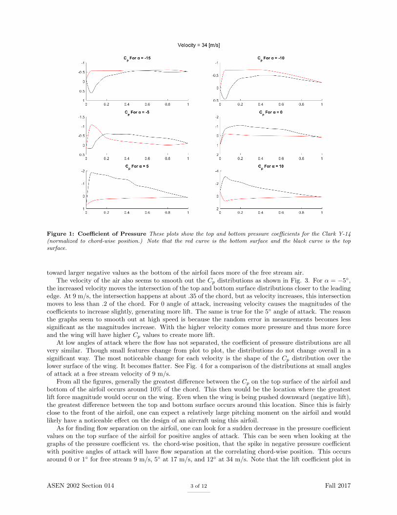
Figure 1: Coefficient of Pressure These plots show the top and bottom pressure coefficients for the Clark Y-14(normalized to chord-wise position.) Note that the red curve is the bottom surface and the black curve is the topsurface.

toward larger negative values as the bottom of the airfoil faces more of the free stream air.The velocity of the air also seems to smooth out the Cp distributions as shown in Fig. 3. For α = −5◦,

the increased velocity moves the intersection of the top and bottom surface distributions closer to the leadingedge. At 9 m/s, the intersection happens at about .35 of the chord, but as velocity increases, this intersectionmoves to less than .2 of the chord. For 0 angle of attack, increasing velocity causes the magnitudes of thecoefficients to increase slightly, generating more lift. The same is true for the 5◦ angle of attack. The reasonthe graphs seem to smooth out at high speed is because the random error in measurements becomes lesssignificant as the magnitudes increase. With the higher velocity comes more pressure and thus more forceand the wing will have higher Cp values to create more lift.

At low angles of attack where the flow has not separated, the coefficient of pressure distributions are allvery similar. Though small features change from plot to plot, the distributions do not change overall in asignificant way. The most noticeable change for each velocity is the shape of the Cp distribution over thelower surface of the wing. It becomes flatter. See Fig. 4 for a comparison of the distributions at small anglesof attack at a free stream velocity of 9 m/s.

From all the figures, generally the greatest difference between the Cp on the top surface of the airfoil andbottom of the airfoil occurs around 10% of the chord. This then would be the location where the greatestlift force magnitude would occur on the wing. Even when the wing is being pushed downward (negative lift),the greatest difference between the top and bottom surface occurs around this location. Since this is fairlyclose to the front of the airfoil, one can expect a relatively large pitching moment on the airfoil and wouldlikely have a noticeable effect on the design of an aircraft using this airfoil.

As for finding flow separation on the airfoil, one can look for a sudden decrease in the pressure coefficientvalues on the top surface of the airfoil for positive angles of attack. This can be seen when looking at thegraphs of the pressure coefficient vs. the chord-wise position, that the spike in negative pressure coefficientwith positive angles of attack will have flow separation at the correlating chord-wise position. This occursaround 0 or 1◦ for free stream 9 m/s, 5◦ at 17 m/s, and 12◦ at 34 m/s. Note that the lift coefficient plot in


Figure 2: Group 1 Angles of Attack These are the coefficients of pressure distribution for the angles of attackmeasured by Group 1. The red curve is the bottom surface of the airfoil while the black is Cp values for the top surface.

Fig. 5a corroborate these observations.


Figure 3: Velocity Effects on Cp These plots show how velocity affects the pressure coefficient distributions forthree angles of attack.

Figure 4: CP Distribution at Small Angles of AttackThese plots show how the pressure distribution for smallangles of attack does not change much while the flow is mostly still attached to the body.


V. Lift and Pressure Drag Coefficients

For all the test data gathered in section 014, the coefficients of lift and drag as a function of angle ofattack are plotted in Fig. 5. Also included in the graphs are NACA test results from Technical Report 628[4].

(a) Coefficient of Lift This plot shows how the coeffi-cient of lift changes with angle of attack at a few differentvelocities.

(b) Coefficient of Drag This plot shows how the co-efficient of drag changes with angle of attack at a fewdifferent velocities.

Figure 5: Coefficients of Lift and Drag

From Fig. 5a it can be seen that the coefficient of lift generally increases with increasing angle of attack.At angles of attack near 0, the lift coefficients for every velocity increase almost linearly. At higher anglesof attack the lift coefficient decreases suddenly. This is the point of trailing edge stall where the sudden lossof lift occurs due to flow separation. As evident in Fig. 5a, the stall occurs later for higher velocities. Foreach measured velocity, the lift coefficient continues to rise after the drop-off, however. This is not quite thesame linear slope, and the lift coefficients appear to resume another linear regime once flow has separated.The regime at extremely low angles of attack is a loss of lift since the angle of attack is too steep. This isleading-edge stall, and all velocities react similar to this effect.

The coefficient of drag also increases with angle of attack above large negative angles of attack (around-7◦). The drag coefficient increases in a non-linear fashion, however. The nonlinear nature of the dragcoefficient curve indicates exponentially increasing drag as angle of attack is increased. At the angles whereleading edge stall occurred in Fig. 5a, the drag coefficient is larger. The flow separation causes not onlydrops in lift, but there is high pressure drag at these angles of attack.

Taking all of this into consideration, the maximum coefficient of lift this Clark Y airfoil produced is 1.5.This occurs at an angle of attack of 11 to 12◦ and a free stream velocity of 34 m/s. This coefficient is highlydependent on tunnel velocity. As shown in Fig. 5a, the higher free stream velocities stay attached to theairfoil at higher angles of attack.

At zero angle of attack, the Clark Y-14 airfoil creates a positive lift coefficient no matter the measuredvelocity. The reason the airfoil creates lift with no angle of attack is due to the camber of the airfoil. At 0angle of attack symmetric airfoils generate no lift, but a cambered airfoil produces an asymmetrical pressuredistribution; the air moves faster over the top of the wing and with the higher local velocity comes lowerpressure. As a result, the total pressure over the top of the wing is less than the pressure acting on thebottom surface and thus lift is generated. Zero lift is generated when the angle of attack is less than zero(which counteracts the camber). This angle ranges from around -9◦ to about -4◦, depending on the freestream velocity.

Though close to the NACA data, the data in Fig. 5a lie slightly above the NACA data. One possiblereason for this slight discrepancy is blockage effects. Since the airfoil blocks a significant amount the testsection in this wind tunnel, the airfoil almost acts as a nozzle in the tunnel and affects the static pressureat a point on the wing. One crude way to start correcting this effect is to scale down the coefficient of liftby the open area of the test section: Atest−Ablocked

Atest. When the coefficients of lift are adjusted in this way,

the plot in Fig. 6 is obtained. Though this does not fully solve the disparity in the data from the NACA


results, one can see this plot is closer to the expected results.

Figure 6: Corrected Lift CoefficientThese are the lift coefficients corrected for blockage in the test section causedby the airfoil as it gets higher angles of attack.

VI. Conclusions

When compared to the 1938 NACA data, the findings in this lab are largely similar, but do have somekey differences. For the lift coefficient, the NACA data for a velocity of 21.4 m/s appears to show no stall,even at angles of attack upwards of 15. In contrast, the lab data only shows no stall for the low velocity of9 m/s. For 17 and 34 m/s, our data shows stall at angles of attack of about 6 and 12, respectively. For thedrag coefficient, the lab data has a tighter fit to the NACA data, but does not include considerations of theeffect of viscosity, which contributes significantly to drag force. It follows the values slightly more closelythan the lift coefficient, and follows the trend of the data throughout all tested angles of attack much moreclosely. Based on this comparison, this lab does a reasonable job of quantifying lift forces about a ClarkY-14 airfoil, but not as good of a job at determining drag, due to the lack of analysis of viscous forces.


References

1Anderson, John David. Introduction to Flight. 8th ed., McGraw Hill Education, 2016.2Taylor, John Robert. An Introduction to Error Analysis: the Study of Uncertainties in Physical Measurements. 2nd ed.,

University Science Books, 1997.3Farnsworth, John. Aerodynamics of a Cambered Airfoil. 15 Nov. 2017,

learn.colorado.edu/d2l/le/content/215270/viewContent/3291372/View.4Pinkerton, Robert M., Greenberg, Harry. Aerodynamic Characteristics of a Large Number of Airfoils Tested in the Variable

Density Wind Tunnel. Report No. 628., National Advisory Committee for Aeronautics, 1938.


Appendix A: MATLAB Code

1 %ASEN 2002 Lab 22 %Group 13 %Data Ana lys i s45 %Fresh Star t6 c l e a r ; c l c ; c l o s e a l l ;78 %Some Constants9 R = 287 ; %[ J /( kg∗K) ]

10 v e l o c i t i e s =[9 17 3 4 ] ;11 a t tacks = −15:16;12 c = s q r t ( .14665ˆ2 + 3 .5ˆ2 ) ;1314 %Gather a l l data15 nameID = { ' 01 ' , ' 03 ' , ' 05 ' , ' 07 ' , ' 09 ' , ' 11 ' } ;% , '1 3 ' , '1 5 '} ;16 losCps=ze ro s (32 ,16 ,3 ) ; %angle down rows , port a c r o s s columns , v e l o c i t y in 3D171819 f o r i =1: l ength (nameID)20 name=[ ' Ai r f o i lP r e s su r e S014 G ' nameID{ i } ' . csv ' ] ;21 data=x l s r e a d (name) ;22 por t s=data ( : , 7 : end−6) ;23 data = data ( any ( ports , 2 ) , : ) ; %Delete rows o f z e r o s24 p atm=data ( : , 1 ) ;25 t atm=data ( : , 2 ) ;26 a i r spe ed=data ( : , 4 ) ;27 pitotDynamicPres = data ( : , 5 ) ;28 por t s=data ( : , 7 : end−6) ;%Get good data f o r por t s again29 ang le=data ( : , end−5) ;3031 f o r j =1:3 %Each team t e s t e d three v e l o c i t i e s32 inds=not ( abs ( s i gn ( s i gn ( v e l o c i t i e s ( j )−3 − a i r sp e ed ) + s i gn ( v e l o c i t i e s ( j

)+3 − a i r sp e ed ) ) ) ) ;33 %Further subd iv ide by ang le34 f o r k=1:32 %Just check each ang le35 a = at tacks ( k ) ;36 inds2 = ( ang le ( inds ) == a ) ; %i n d i c e s in each v e l o c i t y where the re

i s a s p e c i f i c at tack ang le37 i f sum( inds2 )>0 %t h i s ang le was t e s t e d38 f o r l = 1 :16 %16 port measurements39 pDp = pitotDynamicPres ( inds ) ;40 q = mean(pDp( inds2 ) ) ;4142 por ta l oons = port s ( inds , l ) ;43 deltaP = mean( por ta l oons ( inds2 ) ) ;4445 Cp = deltaP /q ;46 losCps (k , l , j ) = Cp ;47 end48 end49 end50 end51 end


5253 %Chordwise p o s i t i o n s54 pos xc = [ 0 .175 .35 . 7 1 .05 1 .4 1 .75 2 .1 2 .8 2 . 8 2 . 1 1 .4 1 .05 0 .7 0 .35

0 . 1 7 5 ] ;55 samples = [ 6 16 2 6 ] ; %I n d i c e s o f ” a t tacks ” f o r the ang l e s we want to look at56 n=length ( samples ) ;5758 %Plot Cp at a sampling o f attack ang l e s59 f o r i =1:3 %A plo t f o r each v e l o c i t y60 f i g u r e61 f o r j =1:n62 subplot (1 , n , j )63 p l o t ( pos xc ( 1 : 9 ) /c , losCps ( samples ( j ) , 1 : 9 , i ) , 'k ' )64 hold on65 p l o t ( pos xc ( 1 0 : 1 6 ) /c , losCps ( samples ( j ) , 10 : 16 , i ) , ' r ' )66 s e t ( gca , ' Ydir ' , ' r e v e r s e ' )67 subname = s p r i n t f ( 'C p For \x3B1 = %1. f ' , a t tacks ( samples ( j ) ) ) ;68 t i t l e ( subname ) ;69 end70 name = s p r i n t f ( ' Ve loc i ty = %1. f [m/ s ] ' , v e l o c i t i e s ( i ) ) ;71 s u p t i t l e (name) ;72 end737475 %%%%%%%%%%%%%%%%%%%%%%%76 % LIFT AND DRAG COEFFICIENTS77 %%%%%%%%%%%%%%%%%%%%%%%78 c l o s e a l l ;79 c l e a r a l l ;80 c l c81 %Read in data82 C l = ze ro s (3 , 32 ) ;83 C d = ze ro s (3 , 32 ) ;84 aoa = ze ro s (1 , 32 ) ;85 index = 1 ;86 f o r i = 1 :887 num = ( i −1)∗2 + 1 ;88 groups = [ ' 01 ' , ' 03 ' , ' 05 ' , ' 07 ' , ' 09 ' , ' 11 ' , ' 13 ' , ' 15 ' ] ;89 f i l ename = [ ' Ai r f o i lP r e s su r e S014 G ' groups (num:num+1) ' . csv ' ] ;90 data in = x l s r e ad ( f i l ename ) ;91 % Replac ing zero rows92 i f i == 393 data in = [ data in ( 1 : 2 1 9 , : ) ; mean( data in ( 1 : 2 1 9 , : ) , 1 ) ; data in ( 2 2 1 : end , : )

] ;94 e l s e i f i ==895 data in = [ data in ( 1 : 7 9 , : ) ; mean( data in ( 1 : 7 9 , : ) , 1 ) ; data in ( 8 1 : end , : ) ] ;96 end97 %cut t ing up data f o r each aoa98 f o r j = 0 :399 data2 = data in ( j ∗60 + 1 : j ∗60 + 6 0 , : ) ;

100 %cut t ing up data f o r each v e l o c i t y 9 ,17 ,34 m/ s101 f o r k = 0 :2102 data = data2 ( k∗20 + 1 : k∗20 + 2 0 , : ) ;103 [ C l ( k+1, index ) , C d ( k+1, index ) , aoa ( index ) ] = getCo ( data ) ;104 end


105 index = index + 1 ;106 end107 end108 %% Plotting109 % Sort ing data by AOA110 p l o t da ta = [ aoa . / 0 . 0 1 7 4 5 3 3 ; C l ; C d ] ;111 p l o t da ta = sort rows ( p lo t data ' , 1 ) ' ;112 %NACA data113 naca aoa = −8 :2 :16 ;114 l ength ( naca aoa )115 n a c a l i f t = [ − 0 . 1 , 0 , 0 . 2 , 0 . 3 2 , 0 . 4 8 , 0 . 6 2 , 0 . 7 8 , 0 . 9 , 1 . 0 7 , 1 . 2 , 1 . 3 , 1 . 4 2 , 1 . 5 2 ] ;116 naca drag = [ 0 . 0 8 , 0 . 0 5 , 0 . 0 7 , 0 . 1 , 0 . 1 8 , 0 . 2 2 , 0 . 3 , 0 . 3 9 , 0 . 4 9 , 0 . 6 , 0 . 7 1 , 0 . 8 5 , 1 ] ∗ 2 / 1 0 ;117 naca v = 2 1 . 5 ; %m/ s118 % Actua l ly p l o t t i n g i t119 %L i f t120 subplot ( 1 , 2 , 1 )121 l p l o t = p lo t ( p l o t da ta ( 1 , : ) , p l o t da ta ( 2 , : ) , ' g ' , p l o t da ta ( 1 , : ) , p l o t da ta

( 3 , : ) , 'b ' , p l o t da ta ( 1 , : ) , p l o t da ta ( 4 , : ) , ' r ' , naca aoa , n a c a l i f t , 'k ' ) ;122 g r id on ;123 t i t l e ( ' L i f t c o e f f i c i e n t ' ) ;124 x l a b e l ( 'AOA [ deg ] ' ) ;125 legend ( ' 9 m/ s ' , ' 17 m/ s ' , ' 34 m/ s ' , 'NACA 21.5 m/ s ' ) ;126 %Drag127 subplot ( 1 , 2 , 2 )128 d p l o t = p lo t ( p l o t da ta ( 1 , : ) , p l o t da ta ( 5 , : ) , ' g ' , p l o t da ta ( 1 , : ) , p l o t da ta

( 6 , : ) , 'b ' , p l o t da ta ( 1 , : ) , p l o t da ta ( 7 , : ) , ' r ' , naca aoa , naca drag , 'k ' ) ;129 g r id on ;130 t i t l e ( ' Drag c o e f f i c i e n t ' ) ;131 x l a b e l ( 'AOA [ deg ] ' ) ;132 legend ( ' 9 m/ s ' , ' 17 m/ s ' , ' 34 m/ s ' , 'NACA 21.5 m/ s ' ) ;133134 s e t ( l p l o t , ' l i n ew id th ' , 1 . 5 ) ;135 s e t ( d p lot , ' l i n ew id th ' , 1 . 5 ) ;136 s u p t i t l e ( ' L i f t and Drag c o e f f i c i e n t s vs AOA ' )137 %% Forces138 func t i on [ C l , C d , aoa ] = getCo ( data )139 %Coordinates o f por t s in meters , t h i s i n c l u d e s t r a i l i n g edge140 coords = 0 . 0 2 5 4∗ [ 0 , 0 . 1 4 6 6 5 ; 0 . 1 7 5 , 0 . 3 3 0 7 5 ; 0 . 3 5 , 0 . 4 0 1 8 ; 0 . 7 , 0 . 4 7 6 ;

1 . 0 5 , 0 . 4 9 ; 1 . 4 , 0 . 4 7 7 4 ; 1 . 7 5 , 0 . 4 4 0 3 ; 2 . 1 , 0 . 3 8 3 2 5 ; 2 . 8 , 0 . 2 1 8 7 5 ; 3 . 5 , 0 ;2 . 8 , 0 ; 2 . 1 , 0 ; 1 . 4 , 0 ; 1 . 0 5 , 0 ; 0 . 7 , 0 . 0 0 1 4 ; 0 . 3 5 , 0 . 0 1 7 5 ; 0 . 1 7 5 , 0 . 0 3 8 8 5 ] ;

141 c = 0 . 0 2 5 4∗3 . 5 ; %chord in meters142 normal = ze ro s (1 , 16 ) ;143 a x i a l = ze ro s (1 , 16 ) ;144 P dyn = mean( data ( : , 5 ) ) ; %Freestream dynamic p r e s su r e145 d i f f P = mean( data ( : , 7 : 2 2 ) ,1 ) ; %D i f f e r e n t i a l p r e s su r e averages146 aoa = 0.0174533∗ data (1 ,23 ) ; %Angle o f at tack in rad ians147 P t = mean ( [ d i f f P (9 ) d i f f P (10) ] ) ; %T r a i l i n g edge p r e s su r e148 d i f f P = [ d i f f P ( 1 : 9 ) P t d i f f P ( 1 0 : 1 6 ) ] ' ; %i n s e r t i n g t r a i l i n g edge p r e s su r e

in to d i f f P149 f o r j = 1 :16 %i n t e g r a t i n g p r e s s u r e s to get f o r c e s150 dx = coords ( j +1 ,1) − coords ( j , 1 ) ;151 dy = coords ( j +1 ,2) − coords ( j , 2 ) ;152 normal ( j ) = −0.5∗( d i f f P ( j ) + d i f f P ( j +1) ) ∗dx ;153 a x i a l ( j ) = 0 . 5∗ ( d i f f P ( j ) + d i f f P ( j +1) ) ∗dy ;154 end


155 F n = sum( normal ) ; %normal net f o r c e156 F a = sum( a x i a l ) ; %a x i a l net f o r c e157 %Normal and a x i a l f o r c e c o e f f i c i e n t s158 C n = F n/P dyn/c ;159 C a = F a/P dyn/c ;160 %Drag and l i f t c o e f f i c i e n t s161 C l = C n∗ cos ( aoa ) − C a∗ s i n ( aoa ) ;162 C d = C n∗ s i n ( aoa ) + C a∗ cos ( aoa ) ;163 end


Aerodynamics of a Cambered Airfoil · Group 1 - December 13, 2017 Jackson Kistler, ∗ Noah...

Documents

Transcript of Aerodynamics of a Cambered Airfoil · Group 1 - December 13, 2017 Jackson Kistler, ∗ Noah...